FM SIGNAL DETECTION THROUGH AM RECEIVER TIME-DERIVATIVE TECHNIQUES

Submitted in Partial Fulfillment of the Requirements for the Degree of Master of Science in Electrical Engineering

by

John R. Dowalo

The School of Engineering

UNIVERSITY OF DAYTON

Dayton, Ohio

June 26, 1970

Approved:

UNIVERSITY OF CAY i ON LIBRARY

71 04345

ACKNOWLEDGMENTS

It is important to recognize those who have made this paper

possible. First and foremost, appreciation is made to my advisor,

Dr. Donald Lewis. Appreciation is also noted to personnel of ASNAE,

Wright Patterson AFB, without whose encouragement this paper might

not have been completed. Acknowledgment is also given to my typist,

Cindy, for the many hours she has put into the typing of this paper.

ABSTRACT

This paper is concerned with the implementation of detection of

commercial radio FM and AM signals by a single detection device.

Detection of FM signals on an AM radio by time-derivative techniques

(slope detection) and its application to commercial FM/AM radios

will be developed. Subjects to be discussed include current FM

(radio) detection techniques, matching networks, frequency conver­

sion (mixer), filtering of the difference frequency, laboratory

results (detuning of the I.F. transformer) and conclusions.

iii

TABLE OF CONTENTS

Page

Acknowledgments ii

Abstract iii

List of Tables VList of Figures vi

I. Introduction 1

II. Approach: The Integration Problem 5

III. Comparison of FM Detection Techniques 9

IV. Matching Networks 25

V. Mixer Design 33

VI. Difference Filter 39

VII. Laboratory Procedures and Results 49

VIII. Summary and Conclusions 61

Bibliography 66

iv

LIST OF TABLES

Tables Pag

1 Comparison of FM Detectors. 24

2 Varying Load Measurements 31

3 Bandpass Filter Response Values 45

v

LIST OF FIGURES

Figure Page

1. Typical Commercial AM Radio I.F. Response Curve 2

2. FM to FM-AM Conversion 3

3. System Integration 6

4. FM Insertion Point to AM Radio 8

5. Frequency Discriminator 10

6. Tank Circuit "A" Output 11

7. Tank Circuit "B" Characteristics 12

8. Output Characteristic Curve 13

9. Phase Discriminator 15

10. Phase Relationships At Resonance 16

11. Phase Relationships Above Resonance 17

12. Phase Relationships Below Resonance 17

13. Ratio Detector 19

14. AM Radio I.F. Response Curve • 21

15. Slope Detector 22

16. Symmetric Matching Networks 26

17. Reduction of VSWR As A Function Of Attenuation 27

18. "T" Network Analysis 28

19. Symmetric Matching Networks 30

20. Image Impedance vs Load Impedance 32

vi

LIST OF FIGURES - CONTINUED

Figure Page

21. Mixer Networks 35

22. Total Mixer Network 37

23. Low Pass Filter 40

24. Bandpass Filter Circuit 43

25. Bandpass Filter Response 47

26. FM Signal Tap 50

27. Output Signal of Mixer - Filter Combination 52

28. AM Receiver - FM Insertion Point ' 53

29. Response Curve - Tank Circuit #1 55

30. Detuned Response Curve - Transformer Circuit #2 58

31. Response Curve - Transformer Circuit #3 59

32. Required AM I.F. Response Curve 62

vii

I. INTRODUCTION

Detection of a frequency-modulated (FM) signal can be performed

by any number of devices. Among the more popular devices used in

commercial receivers are the discriminator (frequency or phase) and

ratio type detectors. However, detection is not limited to these de­

vices. In fact, any device whose output is the time-derivative of

the input will perform an FM-to-AM conversion and therefore can be

used to detect FM [1]. After FM to FM-AM conversion is made, detec­

tion can be performed by conventional AM detection techniques

(envelope detector). This is known as slope detection or more des­

criptively called pime-derivative detection.

Since the I.F. stage of an amplitude-modulated (AM) signal

commercial receiver has a response curve similar to that shown in

Figure 1, it meets the time-derivative requirements for slope

detection and can be used for FM to AM conversion. Therefore, if

the FM signal can be made to correspond in frequency to the slope of

Figure 1, the AM receiver I.F. and detection circuitry can be used

as an FM detector.

This process of detection is not new to the communications

field. During the late 1940‘s, television sound systems were

changing from AM to FM type transmissions [2]. Rather than installing

new circuitry in existing television sets, a slope detection method

for FM detection was applied. By detuning the I.F. transformer of

1

Figure 1 - Typical Commercial AM Radio I.F. Response Curve

the previously AM circuitry to obtain as linear a slope as possible,

FM detection was accomplished. This is pictorially displayed in

Figure 2.

The effort behind this paper is to apply slope detection tech­

niques to the detection of FM commercial radio transmissions on a com

mercial AM receiver. If such a transition can be successfully per­

formed (with good fidelity), FM/AM receivers can be reduced in their

complexity. The chapters that follow will show the development of

the technique to be used in the laboratory to determine the desired

2

Figure 2 - FM to FM-AM Conversion

results. This development will include the approach to be taken in

this paper, a review and comparison of the more popular commercial FM

receiver detection techniques, the integration problem (matching net­

work, mixer, and difference filter), along with laboratory results

and conclusions.

4

II. APPROACH: THE INTEGRATION PROBLEM

In considering detection of a commercial FM radio signal on a

commercial AM radio, many problems of integration arise. Initially,

the problem is that of acceptance of the FM frequency band (88 MHz

to 108 MHz) by the AM radio (550 KHz to 1600 KHz) circuitry. The

problem also arises of individual station bandwidths. According to

Federal Communication Commission (F.C.C.) regulations, FM radio

stations are permitted a bandwidth of ±75 KHz, while AM radio stations

are permitted a bandwidth of ±10 KHz. Again, the problem of AM

receiver circuitry will not allow acceptance of FM transmitted signals

without distortion, due to band limitation.

Signal strength contributes directly to the integration problem

also. If the signal, as tapped from the FM radio, is not at the

proper voltage level at the point of insertion into the AM radio,

detection will be nil.

The approach that will be used in solving the integration problem

is depected in block diagram form in Figure 3. The following dis­

cussions are with reference to this diagram.

(a) FM Radio. The FM signal source is a commercial FM radio

with an operating band between 88 MHz and 108 MHz. Heterodyning

5

(a) (b) (c) (d) (e)

Figure 3 - System Integration

principles will be utilized to obtain a signal whose frequency will

be applicable to a commercial AM radio I.F. response curve slope as

described in Chapter I. This requires that the signal be centered

at approximately 455 KHz ±75 KHz (approximately 380 KHz if detection

will be performed on the positive slope of the response curve;

approximately 530 KHz if detection will be performed on the negative

slope of the response curve). To simplify matters, instead of

"tracing" the local oscillator with the tuning capacitor of the FM

radio, a constant-amplitude signal generator (set at one frequency)

will be used. This can be done only if the output of the FM radio

(at the point where the signal will be tapped) is constant in fre­

quency (with the exception of the ±75 KHz deviation). Therefore, the

point chosen for FM signal tapping was the final I.F. stage where

the signal, regardless of particular station frequency, is always

10.7 MHz ±75 KHz.

(b) Amplifier. A linear amplifier is used to amplify the low -

level signal from the FM radio output.

(c) Mixer - Local Oscillator. The local oscillator sis fixed at

a frequency of 11.23 MHz. When introduced into the mixer with the FM

signal (10.7 MHz ±75 KHz), sum and difference frequencies are pro­

duced. The difference frequency will be 530 KHz with a deviation of

±75 KHz directly proportional to the FM signal. Rationale for

7

this selection (negative response curve slope detection) will be dis­

cussed in Chapter VI.

(d) Bandpass Filter. A bandpass filter is required for accep­

tance of the 530 KHz ±75 KHz difference frequency from the mixer.

It provides attenuation of the sum frequency as well as the two

original frequencies from the mixer and harmonics that may be present

(e) AM Radio. The processed FM signal is now ready for inser­

tion into the AM radio. Insertion is made at the secondary coil of

the I.F. transformer as shown in Figure 4. FM to AM conversion is

performed at this point. The signal is now ready for conventional

AM detection devices. The tuned station on the FM radio should then

be audible at the output (speaker) of the AM radio. It is antici­

pated that for best reception and least distortion, the I.F. trans-

Throughout the transfer networks from FM radio to AM radio, "T"

resistive type matching networks were employed to provide maximum

signal transfer through the predominately passive networks-

S

III. COMPARISON OF FM DETECTION TECHNIQUES

It is necessary at this point to make a comparison of some of

the most commonly accepted techniques for FM detection against the

proposed slope detection technique herein. This comparison, along

with laboratory data on slope detection, will form the basis for the

conclusions of this paper. It is not the intent of this paper to

perform a detailed analysis of each type of FM detector, but rather

to consider the basic techniques of each detector and compare these

with the proposed slope detection techniques.

Of the methods of FM detection available, the most basic are

the discriminator (frequency or phase) detector and the ratio

detector. The following paragraphs are a description of the technique

of FM detection applied by each of these detectors [3].

Discriminator Detectors

Frequency discriminators are the most basic of FM detectors.

The double-tuned (Crosby) discriminator shown in Figure 5 is a fre­

quency discriminator [3]. The technique used for detection of an FM

signal in this circuit is as follows:

9

!i+

Figure 5 - Frequency Discriminator

a. Incoming FM signals at an I.F. frequency of 10.7 MHz are

amplitude limited through the limiter tube to eliminate any AM that

may be 'hiding"on the FM signal.

b. Tank circuit "A" is tuned to 10.7 MHz with a wide enough band

width so as not to introduce amplitude variations of the FM signal

at this point. The output of this tank circuit is symbolically shown

in Figure 6.

Vb*

Figure 6 - Tank Circuit "A" Output

c. Tank circuit "B" is tuned above 10.7 MHz so as to position

the response curve slope at those frequencies +75 KHz above 10.7 MHz

as shown in Figure 7a. The output is therefore an FM-AM signal as

11

shown in Figure 7b

a) Tank Circuit "B" Response Curve

Figure 7 - Tank Circuit "B" Characteristics

d. Tank circuit "C" is tuned below 10.7 MHz so as to position

the response curve slope at those frequencies -75 KHz below 10.7 MHz

12

The resultant is an FM to FM-AM conversion of the signal similar to

that of tank circuit "B".

e. The remainder of the circuit is simply two envelope detectors

(for AM detection) arranged in such a manner that the output voltages

across and R2 are in opposition. At I.F. resonance frequency

(10.7 MHz) the voltages are equal and the output of the discriminator

is zero. At frequencies above and below 10.7 MHz, however, the

voltage output of the discriminator varies at an audio rate controlled

by the modulation frequency of the original FM signal. The final

characteristic curve for this type of discriminator is similar to

that shown in Figure 8.

Figure 8 - Output Characteristic Curve

13

Phase Discriminator

Phase discriminators are probably the most widely-used type of

FM detector in commercial radio. This type of circuit is also known

as the Foster-Seeley Discriminator. A typical circuit is shown in

Figure 9. The technique used for detection of an FM signal in this

circuit is as follows:

a. Incoming FM signals at an I.F. frequency of 10.7 MHz are

amplitude-limited through the limiter tube to eliminate any AM that

may be "riding" on the FM signal.

b. Tank circuit "A" is tuned to 10.7 MHz with a wide enough

bandwidth so as not to introduce amplitude variations of the FM

signal at this point. The output of this tank circuit is symbolically

shown in Figure 6.

c. Tank circuit "B" is also tuned to 10.7 MHz. Therefore, an

FM to FM-AM conversion is not performed by this discriminator. Of

importance-to this circuit are: 1) the secondary coil is center-

tapped .producing a voltage division C^2 across ^2 an^ ^3 across ^3)»

2) the voltage across L| (Ej) is almost the same across L (E^), and

3) the phase relationship between E2 and Eb and E3 and Ej [3].

d. At resonance (10.7 MHz) tank circuit "B" appears resistive

and the induced voltage and current are in phase as shown in Figure 10

14

AudioOutput

L

Figure 9 - Phase Discriminator

El+E3

Note that E^ in the primary coil and E, the induced voltage in the

secondary coil, are 180° out of phase and also that E£ and E^ while

out of phase by 180° effectively lead and lag the induced current

I by 90°. Therefore, the voltage that appears across Rj and R2

(E^+E^ and E^+E^ respectively) cancel each other and there is no

output from the discriminator.

e. At frequencies higher than resonance, tank circuit "B"

appears inductive and the induced current I lags the voltage by an

amount determined by the modulating frequency as shown in Figure 11.

Therefore the voltage that appears across Ry and R2 will vary at an

audio rate determined by the modulating frequency of the FM signal.

f. At frequencies below resonance, tank circuit "B” appears

capacitive and the induced current I leads the voltage by an amount

16

determined by the modulating frequency as shown in Figure 12.

Figure 12 - Phase Relationships Below Resonance

The voltages that appear across R^ and R2 will still vary at an audio

rate as in the case of frequencies above resonance. However, the sum

of the voltages appearing across Rj and R2 below resonance will be

17

opposite in polarity to the sum of voltages across and R2 above

resonance. The final characteristic curve for this type of dis­

criminator will be similar to Figure 8.

Ratio Detector

Ratio detectors are popular in FM detection circuits that are

not preceded by a limiter. The basic ratio detector is shown in

Figure 13. The technique used for detection of an FM signal in this

circuit is as follows:

a. Tank circuit "A" is tuned to 10.7 MHz with a wide enough

bandwidth so as not to introduce amplitude variations of the FM

signal at this point.

b. Tank circuit "B" is also tuned to 10.7 MHz. Therefore an

FM to FM-AM conversion is not performed by this detector. As a

matter of fact, this circuit has the same phase relationship as

the phase discriminator. However, resistors R^ and R2 do not exist

and therefore the voltage potentials Ej+Ej and Ej+E2 are across C2

and Cj respectively.

c. The diodes are in "series aiding" as opposed to the fre­

quency and phase discriminators. Also, a form of biasing is pro­

duced by the RC circuit at such a long time constant that for all

18

o K

o

Figure 13 - Ratio Detector

AudioOutput

intents and purposes it acts as a battery. The charges (positive or

negative) shown in Figure 13 are constant. Therefore, the sum of

the voltages is always constant and equal to the voltage across R.

The voltages across C4 and C5 vary in proportion to the modulation

of the FM signal.

d. At resonance the voltages across C4 and C5 are equal and the

audio frequency voltage at point "X" is zero with respect to ground.

e. As the FM signal is modulated above and below center fre­

quency, the audio frequency voltage between point "X" and ground

varies in proportion to the modulating signal. The resultant output

has a characteristic curve similar to Figure 8.

f. AM is prevented from affecting the circuit because of the

RC circuit. The RC network maintains a biasing potential on capa­

citors C4 and C5 based on the strength of the incoming signal. If

AM is present on the FM it will attempt to increase the voltages

across C4and C$. However, the biasing effect does not permit this

unbalance (the sum of the voltages across capacitors C4 and C5 equals

the bias voltage). This is due to the long time constant of the RC

circuit which does not permit the voltage across R to change fast

enough to accommodate the AM.

20

Slope Detector

Slope detection is basically conversion of the FM signal to

FM-AM and detection of the AM by rectifier detection techniques

(usually envelope detection). The slope detection circuit used for

FM detection in this paper is shown in Figure 15. The technique

used for detection of an FM signal in this circuit is as follows:

a. The incoming I.F. FM signal is centered at 530 KHz. The

tank circuit is the I.F. tank circuit for an AM radio and is

b. FM to FM-AM conversion takes place due to the centering of

the FM signal on the linear portion of the response curve.

c. The FM-AM signal is now detected by the envelope detector

of the AM radio and is then passed on for audio amplification.

21

K>K)

Figure I5 - Slope Detector

Comparison of the FM detectors described is made in Table 1.

Reference will be made to this Table in arriving at conclusions to

the applicability of slope detection in commercial FM/AM radios in

Chapter VIII.

23

Table 1

Comparison of FM Detectors

XFrequency

DiscriminatorPhase

DiscriminatorRatio

DetectorSlope

Detector

DetectionTechnique

Slope Phase Phase-Ratio Slope

AMDistortion

■ EliminatorLimiter Limiter RC Bias

CircuitLimiter

Number■ Of Tuned■ Circuits

3 2 2 1

OutputChacter-

isticFigure 8 Figure 8 Figure 8 Figure 14

SymmetryBalanceRequired

Crucial for output slope linearity

Crucial if proper phas­ing is to be achieved

Critical for eliminaton of distortion

N/A

PhasingBetween

■ Primary 5 . Secondary

Not crucial for

detectionCritical Critical N/A

Diode, Arrangement

SeriesOpposing

SeriesOpposing

SeriesAiding N/A

Slope Linearity

Good Good Good Poor

24

IV. MATCHING NETWORKS

When two or more electrical networks are integrated to perform

a function, it is ideal to have all network source impedances equal.

This is required for maximum signal transfer with minimum VSWR.

However, such an ideal situation is not always the case. Realisti­

cally, this condition can be realized by placing a matching network

between sources.

It is desired that through a matching network, image impedances

will be equal. To obtain this equality, passive symmetric networks

of the "T", "JI" and "LATTICE" types were considered and are shown

in Figure 16. Z^ and Z2 of Figure 16 are image impedances and are

defined as the impedances looking into either terminals of the

matching network. The matching network selected from the above

mentioned three types of networks would be integrated between the

FM radio - local oscillator - mixer combinations, mixer - bandpass

filter combination, and bandpass filter - AM radio combination.

Since most of the transfer network between FM radio and AM

radio is passive, it is desirable to have a matching network of

little attenuation. This must be directly correlated with minimum

VSWR. Such a correlation can be determined from the nomograph of

Figure 17 [6]. Analysis of Figure 17 indicates that 10 db of attenua

tion would yield the best reduction in VSWR with a minimum value

25

----------------OO--------WWv

rl zi -----

--------------- OO---------------------------------

AAAAA/-----OO-

«<------- Z2

oo

b) "II" Matching Network

-------------oo----------

rl zi-------- >

--------------OO---------

c) "LATTICE" Matching Network

Figure 16 - Symmetric Matching Networks 26

f

10.0

5.0

4.0

3.0 1.04

2.01.91.8

1.06

1.08

1.5 1.10

1.3

1.2

cc3:£

ATTENUATOR (db)

— 0C£S 1.2 co >

1.3

1.10

1.08

1.06

1.04

4

6

8

10

12

14

1.5

1.81.92.0

3.0

Figure 17 - Reduction Of VSWR As A Function Of Attenuation 27

of attenuation. On this basis, the three types of networks were

evaluated.

Considering first the "T" network, a value was assigned resis­

tance (=700) and then evaluated for a transfer function furnish­

ing 10 db of attenuation as shown in Figure 18.

Applying loop analysis one obtains

Ein - (70+Zb)I (1)

Eout ~ Zb1 (2)

E°Ut/Eln ’ Zb/70*ZB (3)

but

Eout/ - 0.316 (for 10 db attenuation)'Ein

(4)

28

therefore

Eout, = 0.316 = ZB (5)bin '70+Zb

ZB = 31.90 (6)

Similar analysis was performed on

with the following results:

"II" network:

"LATTICE" network:

"II" and "LATTICE" type networks

ZA = 2160

ZB = 1000

ZA - 1000

ZB = 192.50

(evaluated)

(assumed)

(assumed)

(evaluated)

To determine the consistancy of image impedance values under

varying loads, Figure 19'was used in evaluating the parameters of

Table 2. The values obtained in Table 2 are plotted in Figure 20.

As can be seen from Figure 20, none of the image impedances for the

various types of networks vary to any great extent. It can then be

concluded that any one of the three type networks could be utilized.

The choice of utilizing the "T" type network was made because

1) consistency of design with the passive "T" type mixer network

as described in Chapter V and 2) resistors with proper resistance

values (commercially available) were satisfactory for this network.

29

216Qaaaaa -oo

loon loon

-OO

b) "II" Matching Network

Figure 19 - Symmetric Matching Networks 30

Table 2

Varying Load Measurements

NETWORK LOAD - Rl(O) IMAGE IMPEDANCEZ(D)

iiyu

0 91.95

100 96.00

300 99.50

500 100.40

1000 101.00

nn"

0 68.40

100 72.70

300 74.40

. 500 75.00

1000 75.60

"LATTICE"

0 131.40

100 137.00

300 141.40

500 142.50

1000 144.35

31

V. MIXER DESIGN

The choice of an appropriate mixer in a heterodyne type system

is essentially critical. Due to the mixer in such a system, unde­

sired signals may be formed if care is not taken initially in design.

For the system (integration circuitry between FM and AM radios)

demonstrated in this paper, a double conversion is actually taking

place. The first conversion is made by the FM radio itself from an

rf input signal to a 10.7 MHz ±75 KHz I.F. signal. At this point

the signal is down converted again by the circuitry of section (c)

of Figure 3.

In heterodyne.type systems, it is standard for the local

oscillator to be higher in frequency than that of the incoming rf

signal. When mixed, their beat frequency becomes the I.F. signal.

However, it is possible for an incoming signal to be higher in

frequency than that of the local oscillator. In this case the beat

frequency may be accepted as a legitimate I.F. signal. This is

known as an image frequency. Also of detriment to a heterodyne type

system are spurious responses due to harmonics of the local oscillator

mixing with rf signals outside the desired input signal. Because

of the double conversion performed by the integration circuitry

between FM and AM radios, characteristics of heterodyning such as

these described, are virtually eliminated. This is partially due

to the circuitry of the FM radio ahead of the I.F. tap but mainly due

33

to the constant frequency input to the mixer of 10.7 MHz ±75 KHz.

It is due primarily to the double conversion of the FM signal,

then, that the design of the mixer in this paper is limited basically

to attenuation and matching with input and output circuitry only.

Constant-impedance mixers were chosen for this paper due to the

constant impedances into the mixer from the FM signal amplifier

and the local oscillator. Of the constant impedance mixers there

can be found a variety of configurations such as "T", "II", bridge,'

coil, etc. The "T" configuration was chosen for its basic simplicity

and availability of resistors. In choosing an arrangement of "T"

networks (i.e. parallel, series, etc) consideration must be given

to both "grounding" problems as well as mixing loss. Two such networks

are shown in Figure 21. In computing mixing loss of the networks

shown in Figure 21, we must consider the following [4]:

Parallel:

Mixing Loss = 20 log^n

where n = number of inputs (=2)

substituting:

Mixing Loss = 20 logjQ2 ■ 6.02 db

Series:

Mixing Loss = 10 log^Q (2n-l)

where n = number of inputs (=2)

substituting:

Mixing Loss = 10 log^Q3 = 4.77 db

(7)

(8)

(9)

(10)

34

a) "T" Network In Parallel

■VAAA-

■AAAA/v

-AAAAA-

r2■aaaaa

-AAAAA-

R

O-

b) "T" Network In Series

Figure 21 - Mixer Networks

From the above calculations, it is readily seen that for minimum

mixing loss the best approach is to use the "series T" network.

However, when considering "grounding" of the mixer, the "parallel T"

network is more desirable. This is due primarily to the grounding

35

problems associated with the integration circuitry between (and

including) the FM and AM radios. A common ground is necessary for

compatibility and is provided by the "parallel T" network. The

"series T" network, on the other hand necessitates having one of the

"T" pads above ground. Therefore, accepting a higher mixing loss for

a more preferred grounding system, the "parallel T" network was chosen

for the mixer circuit.

Since the front end of the mixer chosen is a "T" pad, the value

of "R" in Figure 21a is 100ft. This value was chosen in order to be

consistent with all matching networks (see Chapter IV) of the system.

Therefore all input and output impedances appeared as 100ft to the

mixer and the values of the resistors of the "T" pad were the same

as the resistors of the "T"’s of the system matching networks. In

general, the design equation for the desired mixer network is given

as [4] :

R1 = *2 = R(n-l)/(n+i) (11)

where n = number of channels to be mixed

substituting n = 2; R = 100ft:

Rj = R2 = 100(2-l)/(2+1) = 33.3p, (12)

This network output now supplies mixing of the FM signal and

local oscillator signal. To achieve the desired signal (difference

frequency = 530 KHz), the two signals must be passed through a non­

linear device to obtain sum and difference frequencies. A diode of

low forward impedance was chosen for the nonlinear device.

36

The entire mixer network to perform the desired output signal is

shown in Figure 22.

Figure 22 - Total Mixer Network

The diode of the mixer network essentially performs the function

of modulating the FM signal with the local oscillator signal. Choosing

the FM signal and local oscillator signal as functions of voltage, we

assume the following equations':

ec = \f~2 Ec cos(a)CFM + Mf sin usm )t (13)

em Em cos(wc)t (14)

where ec = FM signal

em = local oscillator signal

37

The voltage function for a nonlinear device is given as:

(15)e, = a~ + o o alei + a2ei2

where

ei = ec + em (16)

substituting:

eo = ao + al[J2Ec cos(o>Cfm + Mfsin w^t + cos(o>c)t]

+a2 t \Z^EC cos(u)cFM + Mfsin wmFM)1 + x/2Em cos(wc)t]2 (17)

evaluating:

eo = ao + cos(wCfm + Mfsin O^t]

+an [ /"2E cos (to )t] +a_ [E 21 +ao[E 211 L\/ m '-c>J 2LcJ 2L m J1---------—r------------- - I----------- 1 I__________ d.c._________

em

+a2[Ec2cos(2Uc)t] +a2[Em2cos 2(0,^ + Mfsin u^t]1------------------------------------1 ‘ 1 1

Second Harmonics

+a2[2EcEm cos(uct -[a)CpMt +Mfsin o^t])]

!------------------------- 1 Difference

i Sum.I-------------------------------------------------------------- 1

+a2[2EcEm cos(u)ct + [wCpMt + Mfsin m^t])] (18)

The above output of the mixer (eQ) is now passed through a bandpass

filter which attenuates all of the above signals except the differ­

ence frequency. This signal is favored by the filter and is passed

on for detection in the AM radio.

38

VI. DIFFERENCE FILTER

At the output of the mixer, filtering is required in order to

select the desired signal (difference frequency) and attenuate the

other signals present. Since the I.F. transformer of the AM radio

performs a filtering function, the difference filter at the output

of the mixer performs additional filtering not necessarily required

but of some benefit in controlling Radio Frequency Interference (RFI)

This filter is, therefore, not primarily concerned with the absolute

filtering of the 530 KHz ±75 KHz signal, but rather an attenuation of

other frequencies outside of this range. Therefore, a general filter

design approach was taken in obtaining a filter to perform the above

described function.

To provide filtering for detection of difference frequencies on

either the positive or negative portion of the I.F. response curve

and also allowing FM signal deviations of ±100 KHz (this includes a

±25 KHz guard band), a filter bandwidth of 600 KHz (measured at the

3 db points) had to be realized. This bandwidth also includes

±50 KHz guard band around the curved portion of the I.F. response

curve (455 KHz ±50 KHz). To reduce harmonics as well as other unde­

sirable signals above and below 455 Kl-lz, a bandpass filter with

center frequency of 455 KHz and 3 db bandwidth of 600 KIIz was con­

sidered to be best suited in meeting all the requirements of the

difference filter.

39

A bandpass filter is readily designed through first designing

a low pass filter with a 3 db down point at a frequency which is

the difference between the desired bandwidth of the bandpass filter

and zero [5]. For consideration in this paper, the 3 db down point

is at 600 KHz as shown in Figure 23a. After the circuit parameters

are determined from the transfer function of the low pass filter, it

is a simple matter of adding a capacitor or inductor in series or

parallel (respectively) that are resonant at the center frequency of

Figure 23 - Low Pass Filter

40

From the circuit of Figure 23b, the following calculations were

made to determine the parameters of the low pass filter:

assume: = resistance of generator = 100ft

Rl = resistance of load = 100ft

performing loop analysis we obtain:

Eout(S) = 100 Ij

(19)

(20)

and

o = - ±i +(-2.+ls)i - ii CS 1 CS 2 CS 3

0 = - 2-1 +(100+2-)I CS 2 CS; 3

Eout<S)/£ fs, = 100I3, ! iEin(s) '(100+—)I - —I

CS 1 CS 2

solving for I2 in Equation (22)

I2 = (100CS+l)I3

solving for 1^ in Equation (21)

2-1 = (—+LS) (100CS+1) I - —I CS 1 CS 3 CS 3

I: = (200CS+100LC2S3+LCS2+l)I3

evaluating Equation (23) from (24) and (26)

E-tS)/Eln(S, • 100I3/ (100+-i-) (200CS+100LC2S3+LCS2+l) I

Co 3

(21)

(22)

(23)

(24)

(25)

(26)

-CLOOCS-l)^

(27)

41

E (S) , 100 ,out / = / . „ , . ,

Ein(S) S3(LC2xl04)+S2(200LC)+S(2xl01*C+L) + 200(28)

substituting S = jw

E 100.out J = /EinO) (j“>) 3(LC2xl01*) + (jai)2(200LC)

(29)

+jw(2xlOt*C+L) + 2OO

dividing numerator and denominator by 100 and separating reals from

imaginaries

E r (jto) / _ 1 / i'E. (jto) ‘ /[2-2LC<o2]+j [-100LC2to3+200Cto+-^]

in ioo-1 (30)

rationalize Equation (30) by complex conjugate multiplication

E * (ju>) , out J '/ “ * / I' [2-2LCto2] 2+[-100LC-2to3+200Cto+j~]2 (31)

E 4. (jto) . out JE. (jto) in1

[2 - 2 LCcu2 ] 2+ [-100LC2w3+200Cu+^]21/2

(32)7

Equation (32) is the transfer function of the low pass filter of the

circuit in Figure 23b. Circuit parameters can now be evaluated using

this equation as follows:

assume: C = O.Olpf = 10 8f

to = 2ir(600xl03) = 37.68xl05

where Rg and are image impedances of the networks into and out of

the filter (see Chapter IV)

and

E,'out / = 0.707(0.5) = 0.3535Ein

(33)

42

where: 0.707 = half voltage point

0.5 = maximum output of filter for D.C. input

substituting Equation (33) and above assumption into Equation (32)

0.3535 = L/[2-2L(10“8)(37.68xl05)2]2+[-100L(10“6)(37.68xl05)3

1/2+200(10“8) (37.68xl05) + — -XU"J L]2

100

evaluating Equation (34) we obtain

L2 - 2.63xlO“5L + 1.61xlO“10 = 0

substituting in the quadratic equation

, 2.6 3x10“5 ±\/6.92x10“10-6.44x10"10L — — "

2

2.63x10“2

(34)

(35)

(36)

(37)

L = 1.315xl0“5 = 13.15yh (38)

The parameters of the desired bandpass filter of Figure 24 can now be

determined.100Q 13.15ph C

43

The following formula and assumption are made for resonance

(39)

assume: u = 2-rr (455xl03) « 2.86x10s

solving for L

2.86xl06 = (40)

solving for C

Lj = 0.0122ph (41)

2.86x10s = 1 (42)

C = 0.009xI0's = 0.009pf (43)

The solution to the transfer function for the bandpass filter is

tedious and is susceptable to many mathematical errors. Therefore,

in order to determine the response curve of the filter, empirical

data was used and is shown in Table 3 and Figure 25. This Table and

Figure were determined by a BPF circuit similar to that of Figure 24

but whose values were as follows:

all capacitors = O.Olpf

all inductors = lluh

These values are a result of commercially-available components.

As can be seen by the filter response curve of Figure 25, the

filter does not meet the desired requirements imposed on it initially

due possibly to changes in parameter values because of commercial

availability. The filter does have some acceptable features, however.

The filter will attenuate those undesirable signals expected from the

44

Bandpass Filter Response Values

Table 3

Frequency(MHz)

Ei(volts)

Eo(volts)

E°/Ei ,Normalized E0/^i = X

201ogX(-db)

00.050 S.O 0.000 0.00000 0.0000 —

00.100 8.0 0.000 0.00000 0.0000 -----

00.200 8.0 0.006 0.00075 0.0176 35.10

00.550 S.O 0.210 0.02630 0.6000 4.44

i 00.400 8.0 0.240 0.03000 0.7050 3.04

00.450 8.0 0.2S0 0.03630 0.8300 1.62

00.475 S.O 0.320 0.04000 0.9420 0.52

00.500 8.0 0.340 0.04250 1.0000 0.00

00.550 8.0 0.340 0.04250 1.0000 0.00

00.550 8.0 0.340 0.04250 1.0000 0.00

00.575 8.0 0.320 0.04000 0.9420 0.52

00.600 8.0 0.300 0.03750 0.8820 1.10

00.650 8.0 0.260 0.03250 0.7650 2.32

00.700 8.0 0.240 0.03000 0.7050 3.04

00.750 S.O 0.230 0.02870 0.6750 3.40

00.800 8.0 0.235 0.02940 0.6910 3.20

oo. , n 0 . .’!,() 0 . o 1 ■'.() 0.7 ',(,() . u,

00.000 8.0 0.280 0.05500 0.8240 1.68

00.950 8.0 0.310 0.03870 0.9100 0.82

01.000 8.0 0.270 0.033S0 0.7950 2.00

45

Table 3 (continued)

Frequency(MHz)

Ei1 (volts)

7--------------

Eo(volts)

E°/e. 5 Normalized [ E0/Ei = X

201ogX(-db)

01.100 8.0 0.140 0.01750 0.4120 7.50

01.200 8.0 0.080 0.01000 0.2350 12.58

01.250 8.0 0.060 0.00750 0.1760 15.10

01.300 8.0 0.050 0.00625 0.1470 16.66

01.400 8.0 0.030 0.00375 0.0882 21.08

01.500 8.0 0.010 0.00125 0.0294 30.64

01.800 8.0 0.008 0.00100 0.0235 32.58

20.000 8.0 0.020 0.00200 0.0470 26.56

25.500 7.2 0.040 0.00556 0.1310 17.66

24.000 7 9 0.050 0.00695 0.1635 15.74

25.000 7.2 0.080 0.01110 0.2620 11.64

26.000 7.2 0.070 0.00972 0.2280 12.84

27.000 7.2 0.050 0.00695 0.1630 15.76

28.000 7.2 0.050 0.00695 0.1630 15.76

29.000 8.0 0.060 0.00750 0.1760 15.10

30.000 8.8 0.040 0.00455 0.1070 19.40

40.000 11.0 0.110 0.01000 0.2350 12.58

43.0D0 5.2 0.0 30 0.00378 0.1360 17.32

45.000 4.4 0.020 0.00455 0.1070 19.40

47.000 4.4 0.030 0.00682 0.1600 15.92

50.000 4.4 0.040 0.00910 0.2140 13.40

46

mixer. If the negative slope of the I.F. response curve is chosen

for detection of the FM signal, the filter is sufficient. The filter

peaks at 530 KHz and is a desirable center frequency point on the

negative I.F. slope. The filter will not greatly attenuate the FM

deviation of 530 KHz ±75 KHz. On the basis of the results shown

here, the filter was determined to be acceptable and detection will

be performed on the negative slope of the I.F. response curve

(530 KHz ±75 KHz).

48

VII. LABORATORY PROCEDURES AND RESULTS

Whenever an engineering idea is theorized, laboratory experimen­

tation is generally accepted as proof of the validity or non-validity

of such an idea. In this transition from an idea to experimental

display, all too often modifications and/or complete changes are

required of the original idea in order to complete the experiment

with usable results. As will be seen, the work described in this

paper is no exception to the above statement.

The initial approach to laboratory demonstration was congruent

with the theory presented in the preceding chapters. The following

is a summary of the laboratory procedures and results:

FM Signal Source

An FM/AM receiver, in the FM mode, was used as the FM signal

source. Tapping of the FM I.F. signal (10.7 MHz ±75 KHz) was

accomplished as shown in Figure 26. The following are the problems

encountered and the solutions to those problems:

Problem - How could the tube for I.F. signal amplifica­

tion be tapped without shorting the plate to ground?

Solution - Two resistors as shown in Figure 26 allow both

high resistance to ground but low resistance for FM signal tapping.

49

191IV 8

Figure 26 - 1

Primary Coil Of Phase Discriminator

Problem - Signal level, as tapped, was only 100 mv.

Solution - Commercial RF amplifier with 20 db and 40 db

of gain.

Mixer

The mixer circuit was first evaluated with two constant ampli­

tude signal generators. Parallel "T" matching networks, as described

in Chapter IV, were used at the output of the signal generators to be

consistent with the design requirements of the mixer. This require­

ment is for both inputs to have an impedance of 100Q. The desired

output was obtained, as displayed by an oscilloscope. Readily apparent

were the original signals (undistinquishable from each other) and

the difference frequency signal. No serious problems were encountered

with the mixer.

Difference Filter

Data was taken on the difference filter (bandpass filter) to

obtain its response curve characteristics. This data is available

in Chapter VI. No serious problems were encountered with the dif­

ference filter. As described in Chapter VI, the filter is acceptable

if the negative slope of the AM I.F. response curve is used for FM

to FM-AM conversion.

51

, Mixer - Filter Combination

The mixer and difference filter were combined and their resul­

tant output observed on an oscilloscope. The output appeared as

shown in Figure 27. As is apparent from Figure 27, the difference

filter was not performing satisfactorily in attenuating the 10.7 MHz

±75 KHz FM I.F. signal. This was not considered critical, however,

due to the filtering action of the AM receiver I.F. circuitry.

Difference Frequency 530 ±75 KHz

10.7 MHz ±75 KHz

Figure 27 - Output Signal Of Mixer - Filter Combination

AM Receiver

The AM receiver circuitry was now approached for possible

location for FM signal insertion (now at 530 KIIz ±75 KHz). As shown

in Figure 28, the AM receiver contained two I.F. transformer circuits

(labeled #2 and #3). Initially, the intent was to insert the signal

52

2.2 meg'WW

ToEnvelopeDetector

ToVolumeControl

Figure 28 - AM Receiver - FM Insertion Point

at point F in tank circuit #1. At point E a switch was placed in

order to turn the AM signal off when an FM signal was applied.

Integrated System

The system was now connected in its entirety. Before turning

the system on, however, a common ground had to be established. The

FM and AM radios wall plugs were two pronged, while the local oscil

lator and measuring instruments were three pronged. Three-to-two

prong adapters were obtained. By connecting the grounds of each

circuit, one at a time with a VOM to measure compatibility, common

grounding was achieved. The following are the problems encountered

in obtaining a workable system and the solutions to those problems:

Problem - After hook up and turn on of all systems, no

sound was heard on the AM speaker.

Solution - Adjust voltage level of local oscillator and

also tune local oscillator. This approach had negative results.

Solution - Check output signal of filter just prior to

insertion in the AM radio. Oscilloscope showed that the signal was

proper.

Solution - Check response curve of tank circuit #1. This

result is shown in Figure 29. At this point consideration was

given to two points:

1. Response curve showed that conversion could not

take place at 530 KIIz.

54

2. Low impedance of the difference filter could

destroy the "Q" of tank circuit #1.

Solution (reference Figure 28) - Insert FM signal at the

grid of the I.F. amplifier tube (point *'D"). Place on/off switches

at points "A", "B" and ”C". The signal was now applied with no posi

tive results.

Solution - Excessive attenuation of the signal between FM

and AM radios was next considered. Since the difference filter con­

tained at least 20 db of attenuation, it was removed (keeping in

mind that the AM radio I.F. tank circuit #2 would only respond to

the 530 KHz ±75 KHz signal from the mixer). No positive results

were reached.

Solution - Additional attenuation was taken from the

circuitry with the removal of the "T" networks between the local

oscillator-mixer combination and FM radio-mixer combination. The

attenuation of the mixer, as calculated in Chapter V, would be

changed by not keeping the signal inputs at the same impedance.

However, the difference in attenuation by taking the "T" networks

out was successful in permitting the system to operate properly.

The system operated as expected, with some distortion in the

output signal as heard on the AM speaker. Detuning of I.F. trans­

former circuit #2 was now in order. A level was found where maxi­

mum signal and least distortion were reached. This was only

accomplished after varying the local oscillator frequency from the

original 11.23 MHz to 11.10 MHz. The response curve of the detuned

56

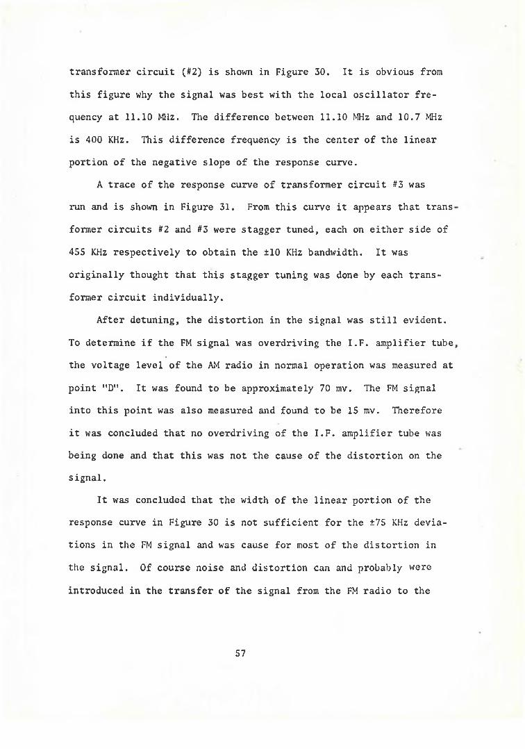
transformer circuit (#2) is shown in Figure 30. It is obvious from

this figure why the signal was best with the local oscillator fre­

quency at 11.10 MHz. The difference between 11.10 MHz and 10.7 MHz

is 400 KHz. This difference frequency is the center of the linear

portion of the negative slope of the response curve.

A trace of the response curve of transformer circuit #3 was

run and is shown in Figure 31. From this curve it appears that trans

former circuits #2 and #3 were stagger tuned, each on either side of

455 KHz respectively to obtain the +10 KHz bandwidth. It was

originally thought that this stagger tuning was done by each trans­

former circuit individually.

After detuning, the distortion in the signal was still evident.

To determine if the FM signal was overdriving the I.F. amplifier tube

the voltage level of the AM radio in normal operation was measured at

point "D". It was found to be approximately 70 mv. The FM signal

into this point was also measured and found to be 15 mv. Therefore

it was concluded that no overdriving of the I.F. amplifier tube was

being done and that this was not the cause of the distortion on the

signal.

It was concluded that the width of the linear portion of the

response curve in Figure 30 is not sufficient for the ±75 KHz devia­

tions in the FM signal and was cause for most of the distortion in

the signal. Of course noise and distortion can and probably were

introduced in the transfer of the signal from the FM radio to the

57

AM radio by the integration circuitry. However, the signal was

easily recognizable as the FM station signal. The distortion noticed

in the signal was similar to the distortion noticed when any radio

is tuned slightly off frequency.

60

VIII. SUMMARY AND CONCLUSIONS

The implementation of detection of commercial radio FM and AM

signals by a single detection device was proven to be feasible.

Integration circuitry was developed in order to obtain the desired

results. These results will now be applied in order to formulate

application of an FM-AM detection device (AM I.F. response curve with

associated envelope detector circuitry) to current FM/AM radios.

Table 1 of Chapter III will be referenced in support of slope detection

over other means of FM detection referenced.

As was expected, some distortion of the FM signal was audible

after detection on .the AM receiver circuitry. This was due primarily

to the poor linearity of the detuned AM I.F. response curve. On the

linear portion of this curve only an FM bandwidth of 30 KHz to 70 KHz

could be realized with any degree of linearity. It can be concluded

that the AM circuitry had the capability of FM detection but not

with a resultant audio signal fidelity that is normally associated

with FM receivers. This problem could be resolved by redesign of

the AM I.F. transformer circuitry to yield a response curve similar

to that shown in Figure 32. This curve could probably be realized

with a tuned transformer circuit similar to the AM I.F. transformer

circuit or a bandpass filter with skirts similar to the difference

(bandpass) filter developed in Chapter VI. However, in order to

reduce undesired responses outside of the 455 KHz ±10 KHz bandwidth,

61

the AM input signal would have to be of a very low level. This is

because of the wide bandwidth associated with the response curve below

the -3 db points.

Double conversion of the FM signal, as performed in this paper,

would not be necessary. This is based on the signal fidelity estab­

lished by current FM radios, of the type used in this paper, that do

not incorporate double conversion techniques. Single conversion

could be made from the rf signal to an I.F. frequency of 370 KHz or

540 KHz, depending on the design of the AM I.F. transformer (reference

Figure 32).

The results of this paper have shown that the difference filter

is not required. Any RFI problems that it might have solved were

not readily apparent. The RFI problems that were encountered were

not due to undesired signals generated by the mixer, but rather to

long connector cabling and inadequacies of breadboard type construc­

tion.

Matching networks were a considerable problem in this paper.

The attenuation offered to the system by these networks proved intol­

erable. The low VSWR and maximum signal transfer they offered the

system did not compensate for the attenuation they provided. Matching

networks were removed from the L.O. - mixer combination, the FM I.F.

signal - mixer combination, and the mixer - AM radio combination

resulting in total system operation without noticeable degradation.

In referring to Table 1, several points are to be brought out in

favor of the slope detector (AM I.F. transformer and associated

envelope detector). Symmetry balance, phasing between primary and

63

secondary, and diode arrangement are not applicable to the slope

detector but are crucial (except for phasing in the frequency dis­

criminator) to present FM detection devices. The number of tuned

circuits is limited to one (possibly two for a stagger-tuned type

transformer) in a slope detector and insures the possibility of less

chances of inadequate tuning of circuitry. Poor linearity appears

to be the only relatively bad feature of the slope detector. This

was brought out quite noticeably in the results of Chapter VII

(distortion of the audio signal). This could be corrected with the

design of a circuit having a response curve similar to that of

Figure 32.

From the results of Chapter VII and the discussions thus far,

it can be concluded that FM/AM radios with a singular detection

device are feasible if modifications are made as follows:

- Eliminate from (present) FM/AM radios -

1. FM detection device

2. AM I.F. transformer

3^ Local oscillator

4. FM I.F. transformer (10.7 MHz)

- Incorporate into (new) FM/AM radio -

1. Circuit to yield a response curve similar

to Figure 32

64

2. Local oscillator

3. FM I.F. transformer to accommodate new

I.F. frequency

As can be seen, more circuitry is eliminated than is incorporated in

the FM/AM radio. The result is less circuitry for an FM/AM radio

employing a single detection device. The resultant fidelity should

be comparable to present FM radios of the type used in this paper

(G.E. models T225A, T235A, and T236A). This statement is made

making note of the slightly distorted audio signal developed in

this approach. If such good quality in an audible signal could

be detected with the poor linearity of the AM I.F. transformer

used in this paper, it is anticipated that good fidelity with redesign,

as noted in this chapter, can be achieved.

In conclusion, this paper has shown the following: 1) Feasi­

bility of single detection of commercial FM and AM signals;

2) Circuit requirements to perform single detection; and 3) Benefits

of single detection to present FM/AM radios.

65

BIBLIOGRAPHY

1. Carlson, A. B. Communication Systems - An Introduction To Signals And Noise In Electrical Communication. New York: McGraw-Hill Book Co., Inc., 1968.

2. Television - How It Works. New York: John F. Rider Publisher, Inc., 1948.

3. Rider, J. F. and Uslan, S. D. FM Transmission And Reception. New York: John F. Rider Publisher, Inc., 1948.

4. Radiotron Designer's Handbook. Australia: Amalgamated Wireless Valve Company Pty. Ltd., 1952.

5. Stewart, J. L. Circuit Theory and Design. New York: John Wiley and Sons, Inc., 1956.

6. Nomograph: Reduction Of VSWR As A Function Of Attenuation.New York: Polytechnic Research And Development Co., Inc.

u a 2KV4 ov66