Flow Boiling of a Dilute Emulsion in the Transition Regime
73
i Flow Boiling of a Dilute Emulsion in the Transition Regime A THESIS SUBMITTED TO THE FACULTY OF GRADUATE SCHOOL OF UNIVERSITY OF MINNESOTA BY AMEYA WAIKAR IN PARTIAL FULFILLMENT OF THE REQUIREMENTSS FOR THE DEGREE OF MASTER.S FRANCIS A. KULACKI, ADVISER May 2020
-
Upload
khangminh22 -
Category
Documents
-
view
6 -
download
0
Transcript of Flow Boiling of a Dilute Emulsion in the Transition Regime

i
Flow Boiling of a Dilute Emulsion in the
Transition Regime
A THESIS
SUBMITTED TO THE FACULTY OF GRADUATE SCHOOL
OF UNIVERSITY OF MINNESOTA
BY
AMEYA WAIKAR
IN PARTIAL FULFILLMENT OF THE REQUIREMENTSS
FOR THE DEGREE OF
MASTER.S
FRANCIS A. KULACKI, ADVISER
May 2020

ii
© Ameya Waikar

i
ACKNOWLEDGEMENT
I would like to thank my parents, Milind Waikar and Yogita Waikar for making huge
sacrifices and supporting me for my education till now. I fall short of words to express my gratitude
to both of you. I know we are thousands of kilometers away physically, but I still feel your blessings
and support emotionally. Thank you for teaching me the importance of learning, education, hard
work, personal responsibility and last but not the least cooking. My journey as a graduate student has
been a rigorous one, it has not only vastly increased my knowledge of fluid mechanics and heat
transfer but also has helped me develop my personality and I come out of this journey as a much
better person than I came in. And I thank both of you to nudge me in this direction, I could not have
asked for anything better.
I would also like to thank all the Professors who taught me the advanced courses in fluid
mechanics, heat transfer, turbulence and CFD. I have learned a lot from all of you. I also thank my
adviser, Professor Dr. Francis Kulacki. Over the two years, I was his student, his TA and his graduate
student and I was happy to have served all these roles in your tutelage . You gave me significant
guidance as well as granted me lot of freedom of decision making about this thesis. I have learned a
lot from you not only about Heat conduction and separation of variables but about US politics, world
politics, philosophy and I am glad to have you as my adviser for this journey.
Next, I would like to thank my colleagues and friend I have made after starting my journey
here. I came to this far away country with no friends, but you guys made sure that I never felt lonely
or home sick. You have taught me the importance of having a good social life. All our conversation
right from gossips to intellectual philosophical discussions about nature of consciousness have left an
everlasting mark on me.
Finally, I would like to thank and express my gratitude to the people who are keeping the
world running and saving lives in these testing times. Thank you to all the medical professionals,
essential service providers, people working at pharmacies and grocery stores, cab and truck drivers
who are literally putting their life on the line to make sure that the rest of us to live comfortably . I am
forever grateful for taking such a huge risk on your lives and making our life relatively comfortable.

ii
DEDICATION
I am dedicating this thesis to my parents and my sister. I am grateful for having a nurturing
family. I also dedicate this thesis to all the people who have succumbed to the horrible disease of
COVID-19. Every human life is valuable and the deaths of so many people by this horrifying disease
is very saddening. May their souls rest in peace .

iii
ABSTRACT
This investigation investigates heat transfer of water and flow boiling of dilute emulsion in
transition and turbulent regime. The gap heights for microgap of 500 and 1000 µm and nominal
Reynolds number of 1600 and 2800. The emulsion in this study is an oil-in-water emulsions, where
FC-72 is the oil whose droplets are suspended in water. The volume fractions for the emulsions are
1% and 2%.
The heated test section is smooth. For single phase experiments, the heat transfer coefficient
of water with increasing Reynolds number and decreasing the hydraulic diameter. The Nusselt
number in the single-phase region is correlated to the Reynolds number, Prandtl number and aspect
ratio of the channel. The Nusselt number varies linearly with 𝑅𝑒𝐷ℎ. 𝑃𝑟.
𝐷ℎ
𝐿 .
In emulsion heat transfer on the smooth surfaces, the value of the heat transfer coefficient
increases only for a volume fraction of 2% of the disperse component under certain conditions.
Reducing the concentration to 1% provides no additional benefit and decreases heat transfer
coefficient for all gap sizes and Reynolds number. The 2% emulsion has a larger overall heat transfer
coefficient than that in water for lower hydraulic diameter and higher Reynolds number. The heat
transfer coefficient increases with increasing wall temperature and plateaus at higher wall
temperatures. The interaction between turbulence and boiling is also an area of interest in this
investigation. When the emulsion boils, there is enhanced mixing in the flow, also leading to further
agitation of the flow causing more turbulence. There is significant increase in pressure drop for the
2% emulsion with increasing wall temperature. Based on these observations and the previously
suggested heat transfer mechanism, the following mechanisms are posited: conduction in thin film of
FC-72 which reduces the heat transfer due to lower conductivity of FC-72; enhanced mixing due to
boiling of FC-72 which increases heat transfer; and the boiling further increases the turbulence,
enhancing the convection of the flow.
These effects are quantified by correlations developed by using seven different non-
dimensional parameters, and an empirical correlation is derived for calculating the heat transfer

iv
coefficient for the emulsion. The correlation is a good fit with 93.8% of data lying within ±30% of
the predicted values.
Further conclusions about the mechanisms involved in the flow boiling of emulsions have
been made, and the data set for the flow boiling of emulsions has been further expanded into
transitional and turbulent regimes.

v
TABLE OF CONTENTS
Acknowledgment …………………………………………………………………………………….. i
Dedication ……………………………………………………………………………………............ ii
Abstract……………………………………………………………………………………................. iii
List of tables…………………………………………………………………………………….......... vi
List of Figures…………………………………………………………………………………….......vii
Nomenclature……………………………………………………………………………………........x
1. Introduction……………………………………………………………………….................. 1
2. Literature review……………………………………………………………………….......... 2
2.1 Turbulence in Microchannels………………………………………………………......... 2
2.2 Flow boiling in Microchannels………………………………………………………..... 5
3. Apparatus and Procedure………………………………………………………..................... 15
3.1 Data reduction………………………………………………………................................ 18
4. Results……………………………………………………….................................................. 20
4.1 Pressure drop……………………………………………………….................................. 22
4.2 Single phase heat transfer……………………………………………………….............. 24
4.3 Emulsion heat transfer………………………………………………………................... 29
5. Correlation………………………………………………………........................................... 36
6. Conclusion………………………………………………………........................................... 38
References………………………………………………………..........................................................44
Appendices………………………………………………………........................................................ 45
A. Experimental Apparatus Drawings……………………………………………………………... 46
B. One dimensional resistance model for heat loss………………………………………………….. 49
C. Analytical Solution…..…………………………………………………………………………… 53
D. Experimental data………………………………………………………………………………… 56

vi
List of tables
Table 2.1. Critical Reynolds number for various aspect ratios [6].
Table 3.1. Uncertainty for various parameters involved.
Table 5.1 p-values for the nondimensional quantities involved in (Eqn 5.2)
Table C1 Value of 𝑘𝑝 for various Reynolds number for the 500 micrometer gap for water
Table D1. Experimental data for water 𝐷ℎ = 980𝜇𝑚 and 𝑇𝑖 = 51𝑜𝐶
Table D2. Experimental data for water 𝐷ℎ = 495𝜇𝑚 and 𝑇𝑖 = 51𝑜𝐶
Table D3. Experimental data for 휀 = 1% 𝐷ℎ = 980𝜇𝑚 and 𝑇𝑖 = 51𝑜𝐶
Table D4. Experimental data for 휀 = 1% 𝐷ℎ = 495𝜇𝑚 and 𝑇𝑖 = 51𝑜𝐶
Table D5. Experimental data for 휀 = 2% 𝐷ℎ = 980𝜇𝑚 and 𝑇𝑖 = 51𝑜𝐶
Table D6. Experimental data for 휀 = 2% 𝐷ℎ = 495𝜇𝑚 and 𝑇𝑖 = 51𝑜𝐶

vii
List of Figures
Fig. 2.1. Friction factor and friction coefficient versus Reynolds number [3].
Fig. 2.2. Dye injection imaging [3].
Fig. 2.3. Flow boiling regimes in horizontal pipe with circular heating [7].
Fig. 2.4. Flow map denoting various regimes under various heat flux and Mass flow conditions [8].
Fig. 2.5. Heat transfer of coefficient versus wall temperature [17].
Fig. 2.6. Typical heat transfer coefficients for emulsions compared to those for water [18].
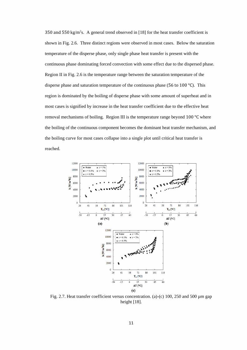
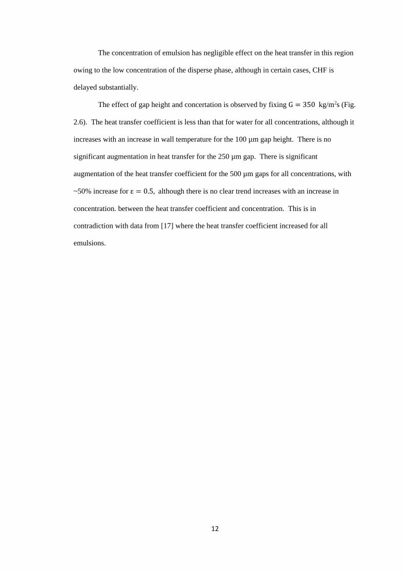
Fig. 2.7. Heat transfer coefficient versus temperature. (a)-(c) for 100, 250 and 500 µm gap heights
[18].
Fig. 2.8. Increase in Heat transfer coefficient versus concentration. (a)-(c) 100, 250 and 500 µm gap
height [18].
Fig. 3.1. Flow loop for the experiments.
Fig. 3.2. Flow loop for emulsion creation.
Fig. 3.3. Droplet size distribution of 1% FC-72-in-water emulsion.
Fig. 4.1. Non-Dimensional Pressure comparison between the experimental data(x’s) and analytical
expression (line), for 𝐷ℎ = 980µ𝑚. (a) Without correcting for other losses. (b) With correcting for
other losses.
Fig. 4.2. Heat loss for calculated from Eqn. (4.3).
Fig. 4.3. Experimental data for pressure drop. 𝐷ℎ = 980 µ𝑚. T = 30°C.
Fig 4.4. Comparison of experimental value of f*Re (x’s) with the theoretical value (line) (Eqn. 4.2).
Dh = 980 μm . Ti = 30°C.
Fig 4.5. Comparison of experimental value of friction factor (x’s) with the theoretical value (line)
(Eqn. 4.2) on a logarithmic scale. Dh = 980 μm. Ti = 30°C.
Fig. 4.6. Heat transfer curves for 𝐷ℎ = 980 µ𝑚. Ti = 51oC.
Fig.4.7. Heat transfer coefficient curves for 𝐷ℎ = 980 µ𝑚. Ti = 51oC
Fig.4.8. Pressure drop curves for 𝐷ℎ = 980 µ𝑚. Ti = 51oC.
Fig. 4.9. Heat transfer curves for 𝐷ℎ = 495 µ𝑚. Ti = 51oC.
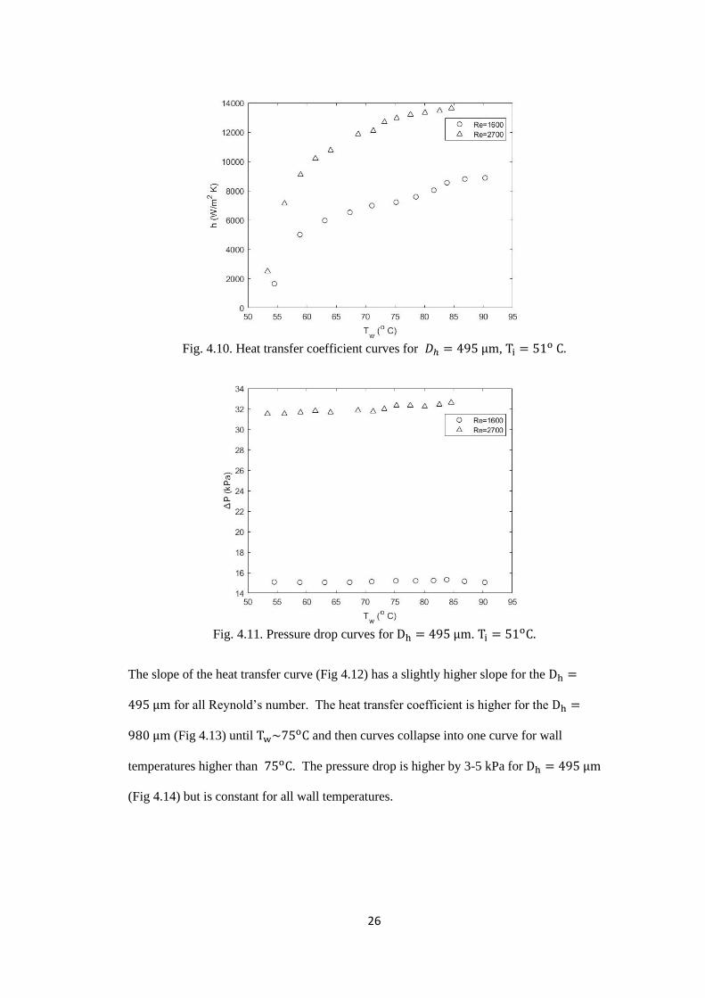
Fig. 4.10. Heat transfer coefficient curves for 𝐷ℎ = 495 µ𝑚. Ti = 51o C.
Fig. 4.11. Pressure drop curves for 𝐷ℎ = 495 µ𝑚. Ti = 51oC.

viii
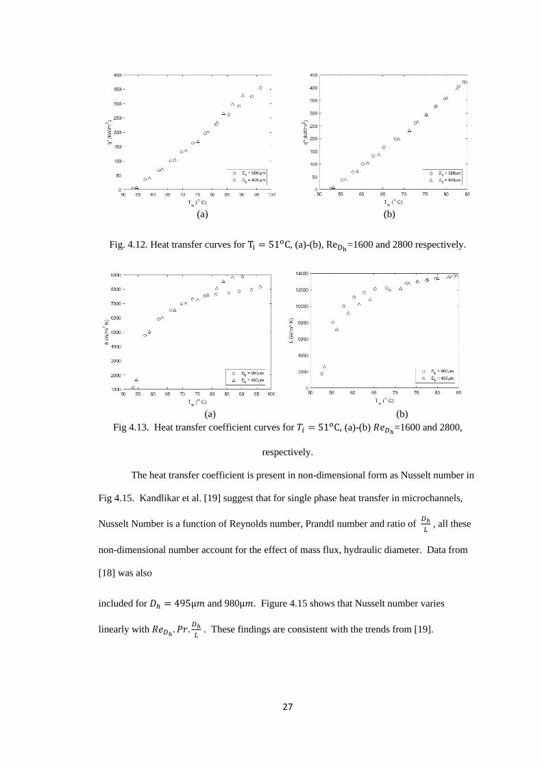
Fig. 4.12. Heat transfer curves for Ti = 51oC, (a)-(b), ReDh= 1600 and 2800 respectively.
Fig 4.13. Heat transfer coefficient curves for Ti = 51oC, (a)-(b) 𝑅𝑒𝐷ℎ=1600 and 2800 respectively.
Fig 4.14. Pressure drop curves for 𝑇𝑖 = 51𝑜𝐶, (a)-(b) 𝑅𝑒𝐷ℎ=1600 and 2800, respectively.
Fig 4.15 Comparison of Nu vs 𝑅𝑒𝐷ℎ. 𝑃𝑟.
𝐷ℎ
𝐿 between B.M Shadakofsky[18], 𝑇𝑖 = 51𝑜𝐶 and this
study.
Fig 4.16. Heat transfer curve for emulsion, for 𝑅𝑒𝐷ℎ= 1600, , 𝑇𝑖 = 51𝑜𝐶 (a)-(b) 𝐷ℎ =
980 µm and 495 µm respectively.
Fig 4.17. Heat transfer coefficient curve for emulsion, for 𝑅𝑒𝐷ℎ= 1600, Ti = 51oC (a)-(b) Dh =
980 µm and 495 µm respectively.
Fig 4.18. Pressure drop curve for emulsion, for 𝑅𝑒𝐷ℎ= 1600, , Ti = 51oC (a)-(b) Dh =
980 µm and 495 µm respectively.
Fig 4.19. Heat transfer curve for emulsion, for ReDh= 2800, , 𝑇𝑖 = 51𝑜𝐶 (a)-(b) 𝐷ℎ =
980 µm and 495 µm respectively.
Fig 4.20. Heat transfer coefficient curve for emulsion, for ReDh= 2800, Ti = 51oC (a)-(b) Dh =
980 µm and 495 µm respectively.
Fig 4.21 Pressure drop curves for emulsion, for 𝑅𝑒𝐷ℎ= 2800, , 𝑇𝑖 = 51𝑜𝐶 (a)-(b) 𝐷ℎ =
980 µm and 495 µm respectively.
Fig 4.22 Heat transfer curves for emulsion for with 𝑇𝑖 = 51𝑜𝐶 (a) ReDh= 1600, ε = 1% (b) ReDh
=
1600, ε = 2% (c) ReDh= 2800, ε = 1% (d) ReDh
= 2800, ε = 2%
Fig 4.23. Heat transfer coefficient curves for emulsion for with 𝑇𝑖 = 51𝑜𝐶 (a) ReDh= 1600, ε = 1%
(b) ReDh= 1600, ε = 2% (c) ReDh
= 2800, ε = 1% (d) ReDh= 2800, ε = 2%
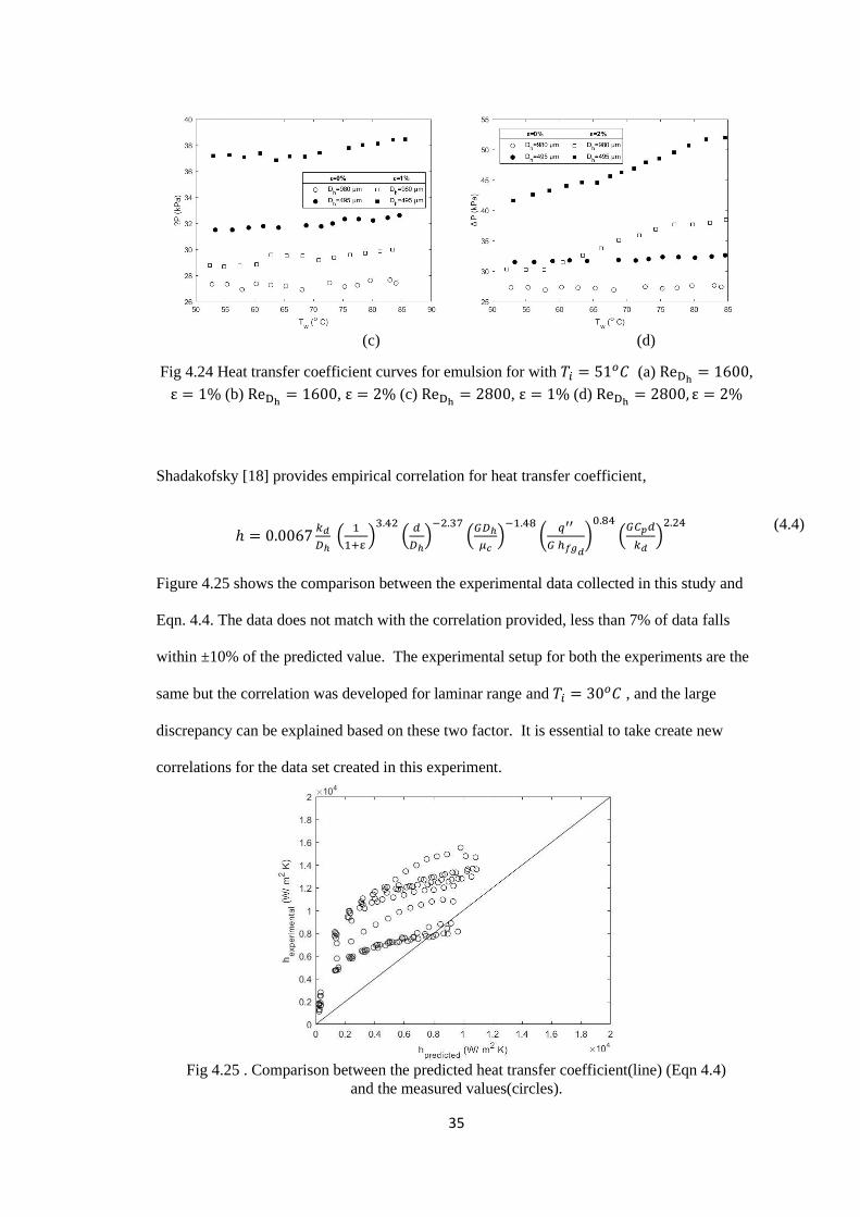
Fig 4.24 Heat transfer coefficient curves for emulsion for with 𝑇𝑖 = 51𝑜𝐶 (a) ReDh= 1600, ε = 1%
(b) ReDh= 1600, ε = 2% (c) ReDh
= 2800, ε = 1% (d) ReDh= 2800, ε = 2%
Fig 4.25 Comparison between the predicted heat transfer coefficient(line) (Eqn 4.4) and the measured
values(circles).
Fig 5.1 Comparison between the measured emulsion heat transfer coefficient and that predicted by
Eqn. (5.2). The solid line represents equivalence between the measured and predicted values. The
dashed line represents ±30% variation from the predicted value.
Fig. 6.1 Ratio of change in heat transfer coefficient to that for water for 𝑅𝑒𝐷ℎ= 1600 on smooth
surface. (a)-(b) are 𝐷ℎ = 495µ𝑚 and 980µ𝑚 respectively
Fig. 6.2 Ratio of change in heat transfer coefficient to that for water for 𝑅𝑒𝐷ℎ= 2800 on smooth
surface. (a)-(b) are 𝐷ℎ = 495µ𝑚 and 980µ𝑚 respectively
Fig 6.3. Map of current data sets for flow boiling of emulsions.
Fig. 6.4 Ratio of change in heat transfer coefficient to that for water for this study, [17] and [18]
Fig. B1. Schematic diagram for resistance network for test section with 𝐷ℎ = 495𝜇𝑚
Fig. B2. Schematic diagram for resistance network for test section with 𝐷ℎ = 980𝜇𝑚

ix
Fig. B3. Schematic diagram for control volume around test section
Fig. C1 Microchannel Geometry

x
Nomenclature
A Area, 𝑚2 δ Uncertainty
𝐶𝑝 Constant pressure specific heat, 𝐽/𝑘𝑔𝐾 ε Dispersed phase volume fraction
𝐷ℎ Hydraulic Diameter, m Subscript
d Droplet diameter, m 0 Reference state
f Friction factor ∞ Ambient properties
g Acceleration due to gravity, 𝑚/𝑠2 analytical Related to the analytical solution
G Mass flux, 𝑘𝑔/𝑚2𝑠 c Continuous component
H Height of the microgap, m cond From conduction
h Heat transfer coefficient, 𝑊/𝑚2𝐾 conv From convection
ℎ𝑓𝑔 Latent heat of vaporization, 𝐽/𝑘𝑔 crit Critical
I Applied Current, A 𝐷ℎ Based on hydraulic diameter
k Thermal Conductivity, W/mK d Disperse component
Nu Nusselt Number, ℎ𝐷ℎ/𝑘𝑓 down Lower surface of channel
P Pressure, Pa f Fluid
Po Poiseuille constant, 𝑓. 𝑅𝑒𝐷ℎ gen Generation
Pr Prandtl number, 𝜇𝑐𝐶𝑝𝑑/𝑘𝑐 in Inlet
q Heat, W loss Value for loss
R Thermal Resistance, K/W m Mean
𝑅𝑢′𝑢′ Autocorrelation of velocity fluctuation max Maximum
𝑅𝑒𝐷ℎ Reynolds Number, 𝜌𝑢𝑚𝐷ℎ/𝜇 net Net value after accounting for losses
𝑅𝑒𝑐𝑟𝑖𝑡 Critical Reynold number for deviation
from laminar flow out
Outlet
T Temperature, 𝐾 TS Related to test section
t Thickness’, m up Upper surface of channel
�⃗⃗� Velocity vector, 𝑚/𝑠 w Wall
u Velocity in X-direction, 𝑚/𝑠 wire Related to wire
u' Velocity fluctuation, 𝑚/𝑠 Superscripts
V Voltage, V ′′ Flux, 𝑚−2
v Velocity in Y-direction, 𝑚/𝑠 Operators
W Width, m ∇ Cartesian gradient operator
w Velocity in Z-direction, 𝑚/𝑠 <A> Average of A
x Streamwise direction . Product
y Normal direction Abbreviation
z Spanwise direction CHF Critical Heat Flux
Greek Symbols ONB Onset of Nucleate Boiling
∆𝑃 Pressure drop, kPa
δ Uncertainty
ε Disperse phase volume fraction
𝜇 Dynamic viscosity, 𝑁𝑠/𝑚2
ν Kinematic viscosity, 𝑚2/𝑠, 𝜇/𝜌
ρ Density, 𝑘𝑔/𝑚3
σ Surface tension, 𝑁/𝑚2
∆𝑃 Pressure drop, kPa

1
1. Introduction
Fluid flow and heat transfer in channel of micro scales (𝐷ℎ < 3𝑚𝑚) have been of
interest because of their application in heat exchangers, fuel cells and most recently for
electronic cooling. Due to ever decreasing size and increasing power density of electronics,
there has been an increasing demand to provide better and efficient cooling on smaller scales.
Better options than gaseous convection demand exploration for the problem of cooling
electronics. Single-phase liquid and two-phase cooling tactics have been explored where flow
boiling in microchannels and microgaps.
Two-phase cooling has been of special interest due to high heat removal capability
that is accompanied with phase change. Most studies for boiling of emulsions are conducted
for pool boiling. Recent studies have conducted experiments to examine the effects of
different parameters on flow boiling of emulsions [12-15]. The parameters that have been
studied are gap size, mass flow rate, concentration of emulsion, droplet size of dispersed
phase, density of the dispersed phase, saturation temperature of dispersed phase and
surfactant used. A detailed review on boiling of emulsions along with mechanisms is
provided in [11]. The field is still very nascent to use them in practical applications. Further
studies are necessary to use this technique for designing .
As a scientist pursuing thermal and fluid sciences, it is essential to have: 1) to study
the physics and parameters involved in flow boiling of emulsions and 2) apply the
understanding to design cooling systems. It is essential to have a detailed data set for
experiments with varying parameters and develop empirical relations for further designing.
To meet these goals, this study aims to:
1. Expand data set of flow boiling of emulsion in microgaps on smooth surfaces into
transition and turbulent regime.
2. Draw conclusions from the experimental data about the physical mechanisms for flow
boiling of emulsions.
3. Suggest further areas of studies and improvements in the field of study

2
2. Literature Review
This research is aimed at understanding boiling of emulsions in microchannels and turbulence
in microchannels. A detailed review of literature in these areas is presented in this section.
2.1. Turbulence in Microchannels
Flow transition in rectangular and circular ducts of conventional sizes with Diameter
greater than 3mm from laminar to turbulent flow has been studied extensively. In the laminar
regime, friction factor is related to the Reynolds number by the equation 𝑓 =Po
𝑅𝑒𝐷ℎ
, where
Po is a Poiseuille’s constant that depends on the geometry of the channel. Shah and London
[1] have calculated values of Po using the analytical solution of the Navier Stokes equations.
This constant for rectangular channels is a function of the aspect ratio.
It is important to verify whether these transition limits at the macro-scale are
applicable in micro-channels as the length scales involved are completely different. Peng et
al. [2], performed experiment with microchannel with gap height ranging from 0.133-0.367
mm and W/H ratio between 1-3 and found the transition to turbulence between 200 < Re <
700. Peng et al. explain this by emphasising the fact that a much smaller value for viscosity is
required to initiate the turbulence in microchannels because wall effects would quickly and
easily penetrate the fluid flow and influence the entire flow. The values for 𝑓. 𝑅𝑒𝐷ℎ showed a
large variation from the theoretical value from equations provided in [1]. They found f to be
proportional to 𝑅𝑒𝐷ℎ
−1.98, which cannot be reproduced in other experiments and is not
consistent with the classical literature. These results might have been unique to the
experimental setup they have used. The details of inlet manifold and the surface roughness
was not been described in the experimental setup.
Pfund et al [3], also investigated pressure drop in microchannels and observe
transition to turbulence for microchannels for channels of heights 128, 263, 521 and 1050 μm,
width of 1 cm and Reynolds numbers from 50 to 3450. The flow transition for the 521 𝜇𝑚
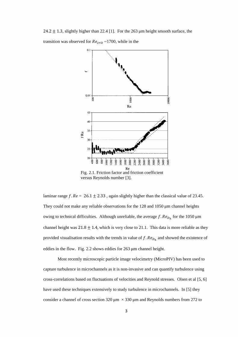
microchannel was observed at 𝑅𝑒𝑐𝑟𝑖𝑡 = 2200 (Fig. 2.1), while in the laminar range 𝑓. 𝑅𝑒𝐷ℎ =
3
24.2 ± 1.3, slightly higher than 22.4 [1]. For the 263 μm height smooth surface, the
transition was observed for 𝑅𝑒𝑐𝑟𝑖𝑡 ~1700, while in the
laminar range 𝑓. 𝑅𝑒 = 26.1 ± 2.33 , again slightly higher than the classical value of 23.45.
They could not make any reliable observations for the 128 and 1050 μm channel heights
owing to technical difficulties. Although unreliable, the average 𝑓. 𝑅𝑒𝐷ℎ for the 1050 μm
channel height was 21.8 ± 1.4, which is very close to 21.1. This data is more reliable as they
provided visualisation results with the trends in value of 𝑓. 𝑅𝑒𝐷ℎ and showed the existence of
eddies in the flow. Fig. 2.2 shows eddies for 263 μm channel height.
Most recently microscopic particle image velocimetry (MicroPIV) has been used to
capture turbulence in microchannels as it is non-invasive and can quantify turbulence using
cross-correlations based on fluctuations of velocities and Reynold stresses. Olsen et al [5, 6]
have used these techniques extensively to study turbulence in microchannels. In [5] they
consider a channel of cross section 320 μm × 330 μm and Reynolds numbers from 272 to
Fig. 2.1. Friction factor and friction coefficient
versus Reynolds number [3].

4
2853. They used the values of ensemble average of velocity fluctuations as the measure of
turbulence and observed increase in < 𝑢′ >/𝑢𝑚𝑎𝑥 at 𝑅𝑒𝐷ℎ= 1535. The flow is fully
developed flow for 2630 < 𝑅𝑒 < 2835. Based on the rapid decrease of auto-correlation in u
velocity, 𝑅𝑢′𝑢′, when compared to flow in macro scales, the flow is more turbulent in nature.
In [6], similar analysis was done for rectangular channels with W/H ratio from 0.97 to 5.69
and 200 < 𝑅𝑒𝐷ℎ< 3267. Following is the table for the values of aspect ratios and
corresponding Reynolds number where transition was observed
Table 2.2. Critical Reynolds number for various aspect ratios [6].
W/H Recrit
0.97 1885
2.09 2315
3.05 1765
4.00 1867
5.69 1837
Fig. 2.2. Dye injection imaging [3].

5
There is no clear trend regarding the variation of 𝑅𝑒𝑐𝑟𝑖𝑡 with aspect ratio, but these
values fall well within the classical range of 1800 -2300 . The aspect ratio affects the
uniformity of flow in transverse direction, because for the lower W/H, the effect of side wall
is very prominent. Based in the velocity profiles, the flow becomes fully turbulent for all of
these aspect ratios for 2600 < 𝑅𝑒𝐷ℎ< 3000.
2.2. Flow Boiling in Microchannels
It is important to discuss flow boiling in general before getting into specifics of flow
boiling of emulsions. Flow boiling is a gas-liquid two-phase flow where the dispersed gas
phase is developed in situ by vapour formation from liquid. Based on vapor quality, the
multiphase flow can be divided into various regimes. With sufficient heating above the
saturation temperature, nucleation begins in the flow. Individual small bubbles are formed at
various nucleation sites and give rise to bubbly flow. Moving downstream or increasing heat
flux causes the flow to transition to slug flow, where the bubbles are agglomerated to form a
large vapour slug, with aerated or unaerated wakes behind it. The slugs are periodic with a
thin film attached to the wall. The slugs flow asymmetrically towards the upper side due to
density stratification. If the heat flux is increased furthermore, the flow transitions to either
wavy or annular flow, depending on the flow velocity. In either case, the liquid film flows at
the bottom and the vapor flows at the top. The flow is classified as either wavy or annular
flow depending on the gas-fluid interface. The interface has ripples if inertia is more
dominant than surface tension and the flow is termed wavy. Annular or stratified flow will be
observed if inertia and surface tension are similar in magnitude and can maintain a stable
interface which is usually observed at lower mass flow rates. As the heat flux increases the
liquid film will evaporate, and the flow transitions to critical heat flux with wall burnout.
These flow regimes are slightly different for microchannels. Harirchian and
Garimella [8] provide flow regime map for boiling of FC-77 in microchannels for 96 ≤ Dh ≤
707 , and W/H ratio of 0.27 to 15.55 with mass flux varying from 225 to 1420 kg/m2s.

6
For smaller microchannels and lower mass and heat fluxes, slug flow is observed unlike for
conventional channels where bubbly
Fig. 2.3. Flow boiling regimes in horizontal pipe with circular heating [7].
flows are observed. Also at higher heat flux, they observed an alternating churn and confined
annular flow with vapor core surrounded by a thin liquid film. Both of these distinctions were
not observed in increased channel cross-sectional areas. They give a flow map for mass
fluxes versus heat flux (Fig. 2.4).
Research in the field of boiling of emulsions is rather sparse. Mori et al. [9] studied
pool boiling of oil-in-water and water-in-oil emulsions on a horizontal wire. KF 96, KF 54,
Dodecane and Undecane were the oils that were used, along with sodium oleate, Tween 80
and Span 80 as emulsifiers. Water-in-oil emulsions require a large surface superheat when
compared to oil-in-water. This is more likely as higher water fraction would be available to
wet the wire and boil. They also discuss the effects of specific emulsifiers which are not
discussed here.
Roesle and Kulacki [10] investigated boiling of FC-72-in-water and pentane-in-water
emulsions on a heated wire with concentrations 0.1, 0.2, 0.5, 1% volume fraction of the
disperse component. They compared their experimental data with the Morgan and Rohsenow
correlation [10] ,
𝐶𝑝(𝑇𝑤𝑖𝑟𝑒−𝑇𝑠𝑎𝑡)
ℎ𝑓𝑔𝑃𝑟= (
𝑞
µ𝑓ℎ𝑓𝑔)1/4
(𝜎
𝑔(𝜌𝑓−𝜌𝑔))1/6
(2.1)

7
For FC-72, the natural convection heat transfer coefficient decreases with increasing volume
fraction of the dispersed component. Shadakofsky and Kulacki [11] attribute this to the fact
that FC-72, which
Fig.2.4. Flow map denoting various regimes under various heat flux and Mass flow
conditions [8].
has higher density that water and settles on the wire and has lower thermal conductivity.
They also observed 35 − 55 oC superheat for boiling FC-72. They observed overshoot in
temperature for boiling of FC-72 for lower concentrations but it is non-existent for a 1%
concentration of the disperse component and attribute this to the lesser rewetting of the wire
at lower concentration. They noted that the superheat made it difficult to separate the effect
8
of FC72 boiling with the boiling of the continuous component. Pentane has a saturation
temperature is 35. 9 oC, which is about 20 oC lower than that of FC-72. For this emulsion the
natural convection heat transfer coefficient is also lower when compared to water, but the
reduction is less than for FC72-in-water. This further strengthens the hypothesis by
Shadakofsky et al. as the density of pentane is lower than water and it does not coat the wire
as much as the FC72. The pentane-in-water emulsion has negligible temperature overshoot
for lower concentrations but very significant overshoot for ε = 0.5 and 1%, although no
satisfactory explanation is provided.
Bulanov et al. [12] and Gasanov and Bulanov [13, 14] discuss the effect of initial
bulk temperature and droplet size on the heat transfer characteristic. Generally, slightly
higher heat transfer coefficient was observed with higher initial bulk temperature. For the
droplet size, coarse grained (20 − 30 μm) or fine grained (1 − 2 μm) were considered.
Although minimal difference is observed the natural convection, but the fine-grained
emulsions require a higher superheat (~70 𝑜𝐶) than coarse grained emulsions. This is to be
expected as the smaller droplets have a larger pressure inside them owing to surface tension,
although this alone cannot be the only factor as the pressure increase would only account for
~10 oC.
Gusanov and Bulanov [15] report one of the first studies in flow boiling of emulsion
albeit in conventional sized peripherally heated pipes with a diameter of 16 mm. They
performed the study of coarse (20 − 30 μm) and fine grained (1 − 2 μm) emulsion of water-
in-VO-1C oil at various concentrations (0.1 ≤ ε ≤ 1.5 ) at a volumetric flow rate of
2.5 × 10⁻⁶m3/s. Both emulsions showed significant increase in the heat transfer coefficient
near the saturation temperature of water. For the same temperature, the fine grained emulsion
required larger superheat when compared for onset of nucleate boiling (ONB). The fine-
grained emulsions also have higher critical heat flux which increases with increased
concentration. Shadakofsky and Kulacki [11] review other studies by Bulanov on flow
boiling of water-in-PES4 emulsion at mass flow rate of ~0.006 𝑘𝑔/𝑠 in a pipe of diameter of

9
8.4 mm with inlet bulk temperature of 60 oC and weight percent of PES-4 between 3 − 33%.
The heat transfer coefficients shift to lower wall temperatures and increase with weight
percent. They also observe boiling occurs at saturation temperature of water which in
contrast to pool boiling which needs superheat.
Roesle and Kulacki [16] and Jansen and Kulacki [17] have studied flow boiling of
oil-in-water emulsions in microgap channels. In [16] they studied gaps of 0.1mm with an
aspect ratio of 300.
Fig. 2.5. Comparison of h for emulsions and water [17].
They performed experiments on single phase (FC-72) and two-phase (FC-72-in-water). The
experimental setup had an inlet well before entering the microchannel but it led to improper
or no
mixing at leading to mostly separated flow and the heat transfer data is inconclusive as there
is no emulsification. In [17], the emulsions were made separately and then ran through the
experimental setup. The gap height was 0.25 mm with an aspect ratio of 120 with a heater at
the length of 60 times of the hydraulic diameter. They studied FC72-in-water and pentane-in-

10
water with concentrations 0.1 < ε < 2, with droplet diameter of the dispersed component
ranging between 5 and 7 µm and bulk inlet temperature of 25 °C. At a mass flow rate of 133
kg/m2s, 20 - 60% enhancement in heat transfer coefficient was observed for FC-72-in-water
emulsions for wall temperatures ~75 to 100 °𝐶 for all concentrations, mostly owing to the
boiling of the FC-72. The wall superheat required for ONB reduced with increase in
concentration. There was no statistically significant change in the heat
transfer coefficient for both 0.1% and 1% concentration even though the saturation
temperature of pentane (36 °C) is less than that of FC-72 (56 oC). They attribute this to the
fact that pentane boils too
Fig 2.6. Typical heat transfer coefficients for emulsions compared to those for water [18].
quickly in the continuous phase before wetting the heated surface, . The comparison between
these are shown in the Fig. 2.5.
Detailed studies of flow boiling of dilute FC72-in-oil emulsions in microgap channels
have been performed by Shadakofsky [18] on smooth and microporous surfaces. The
experimental setup includes gap heights of 100, 250 and 500 µm in a flat channel of 33.4 mm
width. The concentrations used were ε = 0.1, 0.5, 1 and 2% and flow rates were 150,
11
350 and 550 kg/m2s. A general trend observed in [18] for the heat transfer coefficient is
shown in Fig. 2.6. Three distinct regions were observed in most cases. Below the saturation
temperature of the disperse phase, only single phase heat transfer is present with the
continuous phase dominating forced convection with some effect due to the dispersed phase.
Region II in Fig. 2.6 is the temperature range between the saturation temperature of the
disperse phase and saturation temperature of the continuous phase (56 to 100 °C). This
region is dominated by the boiling of disperse phase with some amount of superheat and in
most cases is signified by increase in the heat transfer coefficient due to the effective heat
removal mechanisms of boiling. Region III is the temperature range beyond 100 °C where
the boiling of the continuous component becomes the dominant heat transfer mechanism, and
the boiling curve for most cases collapse into a single plot until critical heat transfer is
reached.
Fig. 2.7. Heat transfer coefficient versus concentration. (a)-(c) 100, 250 and 500 µm gap
height [18].
12
The concentration of emulsion has negligible effect on the heat transfer in this region
owing to the low concentration of the disperse phase, although in certain cases, CHF is
delayed substantially.
The effect of gap height and concertation is observed by fixing G = 350 kg/m2s (Fig.
2.6). The heat transfer coefficient is less than that for water for all concentrations, although it
increases with an increase in wall temperature for the 100 µm gap height. There is no
significant augmentation in heat transfer for the 250 µm gap. There is significant
augmentation of the heat transfer coefficient for the 500 µm gaps for all concentrations, with
~50% increase for ε = 0.5, although there is no clear trend increases with an increase in
concentration. between the heat transfer coefficient and concentration. This is in
contradiction with data from [17] where the heat transfer coefficient increased for all
emulsions.
13
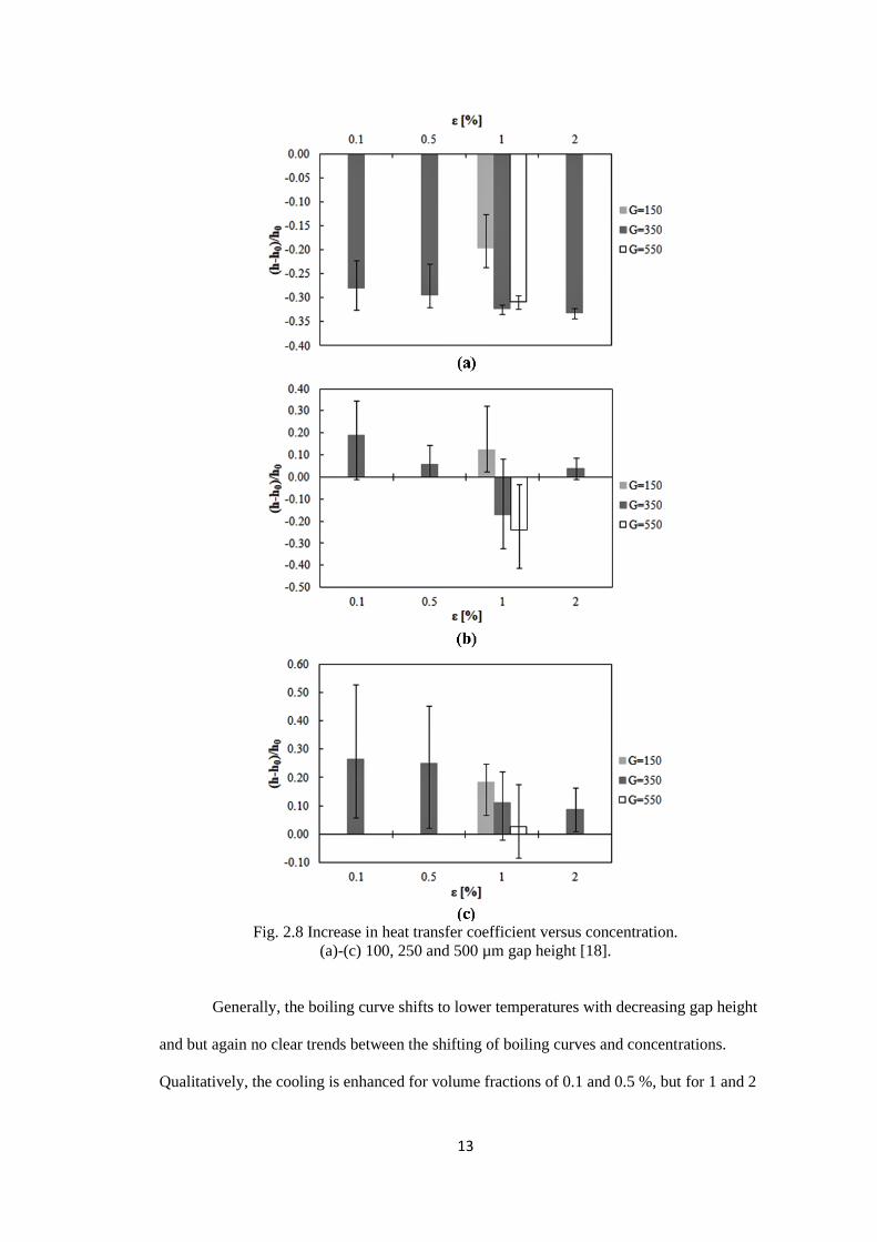
Fig. 2.8 Increase in heat transfer coefficient versus concentration.
(a)-(c) 100, 250 and 500 µm gap height [18].
Generally, the boiling curve shifts to lower temperatures with decreasing gap height
and but again no clear trends between the shifting of boiling curves and concentrations.
Qualitatively, the cooling is enhanced for volume fractions of 0.1 and 0.5 %, but for 1 and 2

14
% show detrimental effects in certain cases. Increased gap size and lower mass flux increases
the heat transfer coefficient when
compared to those in water. Figure 2.8 shows a comprehensive comparison of Heat Transfer
coefficient compared to water under all experimental circumstances.
Shadakofsky thus suggests that there are two heat transfer mechanisms at play in
these experiments. First that enhances heat transfer and other which is detrimental. The
emulsion may form a film on the heater, especially for small gap heights and lower mass
fluxes. In Region I, owing to the substantially lower conductivity of FC-72 when compared
to that of water, the heat removal is less. Heat transfer is enhanced once the dispersed phase
starts boiling, but not beyond the forced convection of water in all cases.

15
3. Apparatus and Procedure
Fig. 3.1. Flow loop for the experiment.
The flow loop is similar to that in [18]. Figure 3.1 below shows the flow loop. It has
two separate flow loops. The recirculation loop is used to increase the temperature of the
fluid in the reservoir to control the inlet temperature. The temperature inside the reservoir is
increased by a heater controlled by a proportional integral derivative (PID), which gets input
from a thermocouple installed in the reservoir. Once the required initial temperature is
reached, the recirculation loop is closed and the fluid flows through the test loop.
The test loop contains a pump with variable-frequency drive motors which pumps the
fluid . The fluid first flows through a rotameter which is used to control the fluid flow rate .
Flow rate is also measured separately by collecting fluid in a beaker while timing it and
measuring the mass of the fluid collected. A needle valve is placed after the rotameter to
reduce the pressure fluctuations during boiling. Pressure transducers and thermocouples are
placed before and after the test section to measure the pressure drop and inlet and outlet

16
temperatures respectively. A heat exchanger is placed after the outlet pressure transducer to
cool the fluid before going back to the reservoir.
The entire test section is machined from Garolite™ to limit heat loss to the
surrounding . The channel is 25.4 mm wide and 275.2 mm long. The entrance and exit
manifolds are angled at 30° (Fig A4) . The test section has an entrance length of 165.95 mm
before the heated part test section which is sufficiently long for having a fully developed
turbulent flow at the highest Reynolds number used in this investigation. All the experiments
were performed on the smooth copper surface polished using P2000 sandpapers. The gap
heights used in this investigation are 250 and 500µm, the Reynolds numbers used were 1600
and 2750 and the concentrations used were 1% and 2%. The 500µm gap also has a
transparent glass window on top. The fluid is pre-heated to a temperature of 51°C before
starting the experiment to reduce the sub-cooling. The designs are presented in Appendix A
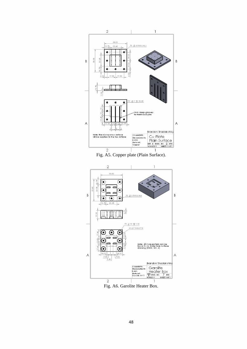
The heater applies a constant heat flux boundary condition in heated region of the test
section. The heater comprises of four Al-Ni heaters with built in thermocouples which are
placed inside a Garolite™ G-101 box. Garolite has low thermal conductivity and limits the
heat loss to surrounding. The heater setup is attached to a copper block using thermal grease .
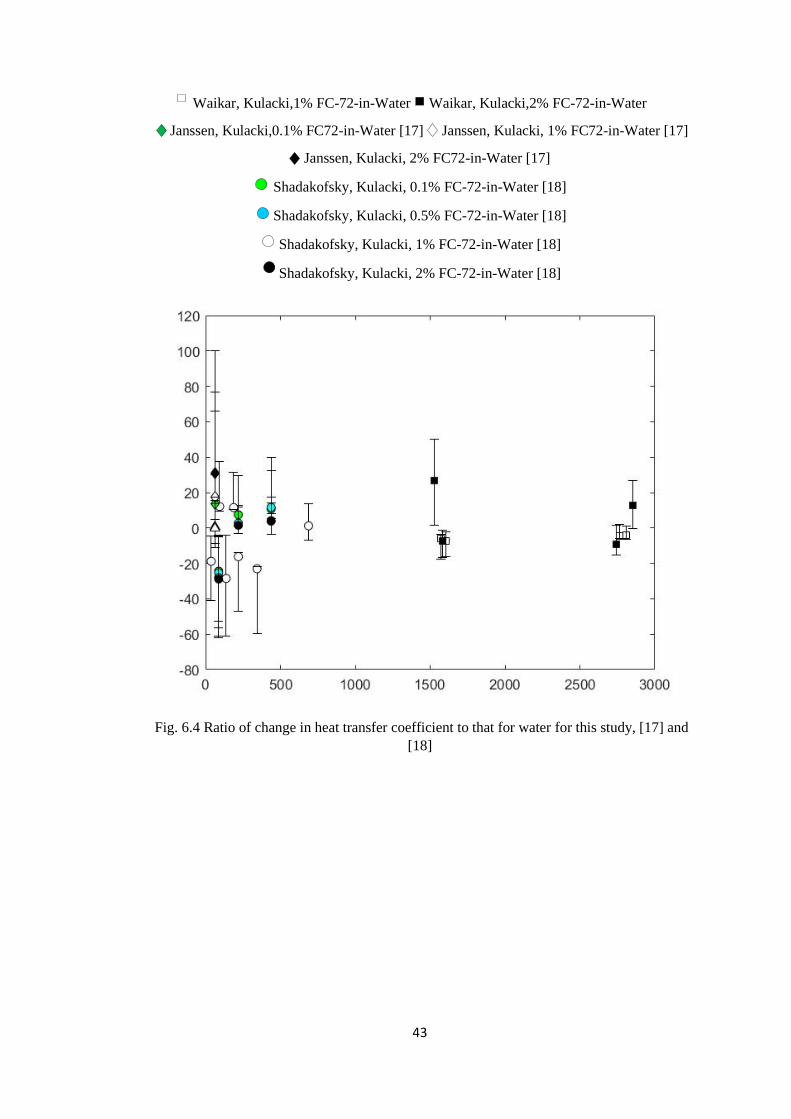
The exposed surface area is 25.4 mm × 25.4 mm . The block has 8 holes drilled 0.5 mm
below the surface exposed to the fluid . These holes hold the E-type thermocouple to measure
the surface temperatures. The copper and heater setup are sealed in the test section using
Clear Super Silicon Sealant by 3M™.
National Instruments (NI) USB 9171 data acquisition device (DAQ) is used to
measure the temperature and NI USB 6000 DAQ is used to measure the pressure drop from
the PX-309 Omega pressure transducer. Data is sampled at 50 Hz for 5 seconds when steady
state is reached.
1 FC-72 is a thermally and chemically stable, dielectric Flourinert™ Electronic Liquid produced by 3M and
intended to be used for leak detection and cooling of electronic equipment. At 1 atm and 25 °C, FC-72 has the
properties ρ = 1680 kg/m3, μ = 64×10-5 Ns/m2, CP = 1100 J/kg°C, and k = 0.057 W/m°C. FC-72 also has a low
saturation temperature (56 °C at 1 atm).

17
The data is acquired using a LABVIEW program which takes the mass flux, heater
surface area, heater input power and heat loss as input and writes out net applied heat flux and
heat transfer coefficient along with mean surface temperature and mean pressure drop.
Fig. 3.2. Flow loop for emulsion creation.
Fig. 3.3. Droplet size distribution of 1% FC-72-in-water emulsion.
The emulsion is created in a separate flow loop (Fig. 3.2). Distilled water is first
degassed by heating in a closed container for 25-30 min. It is then cooled down and the
required amount of FC-721 is added to it. FC-72 and water are immiscible, but they are
emulsified by using a check valve mechanism. The mixture is flown through a check valve at

18
mass flux of 1050 𝑘𝑔
𝑚2𝑠 so that the FC-72 particles are broken down and suspended in water.
The mixture flows through this loop for 5-10 min before being transferred to the fluid
reservoir mentioned in previous sections. The procedure is same as followed in [18]. The
droplet size distribution is non-Gaussian with a mean of 2.54 µm with a standard deviation of
1.027 µm. The distribution in presented in Fig. 3.3
3.1. Data Reduction
Pressure drop measured by the transducers (∆Ptotal) includes the pressure drop due to the
inlet and exit losses as well as the pressure drop along the test section,
∆Ptotal = ∆P𝑛𝑒𝑡 + ∆Plosses (3.1)
The friction factor is calculated using the Eqn. (3.2),
𝑓 = (
ΔP𝑛𝑒𝑡Dh
2ρum2 L
)
(3.2)
And ∆Plosses is given by,
∆Plosses = 𝑘𝑝𝜌um2
(3.3)
The details on the calculation of the value of 𝑘𝑓 is provided in Appendix C.
The heat transfer coefficient is,
ℎ =
𝑞𝑛𝑒𝑡′′
(𝑇𝑤 − 𝑇𝑓)
(3.3)
where the wall temperature is calculated by taking the mean of the temperature’s values
recorded by thermocouples, and the fluid temperature is calculated by taking the average of
inlet and outlet temperature. The uncertainties in the quantities are presented in Table 3.1.
In case of quantities with multiple sources of uncertainty, the total uncertainty is
calculated as the root mean square of the individual uncertainties. For quantities which are
calculated as a function of other parameters, partial derivatives are used to calculate total
uncertainty. An example for this is given by uncertainty in f is given by,
𝛿𝑓 = √(∂𝑓
∂∆PTS𝛿∆PTS)
2
+ (∂𝑓
∂∆V𝛿∆V)
2
,
(3.5)
The uncertainty measurements for various parameters has been mention in Table 3.1.

19
Table 3.1. Uncertainty for various parameters involved.
Quantity Uncertainty
𝑉 ±1.5%
H ±13 μm
I ±1.5%
Q ±3-5%
G
∆𝑃
ε
T
±0.5-3%
±0.2-1.4%
±3-4%
± 1%

20
4. Results
To identify the transition regimes in the test section it is essential to estimate the
pressure drop across the test section. The pressure transducers are placed before and after the
test section. This also includes the pressure drop due to the intermediate pipes, inlet and exit
manifolds. The length of the test section ensures that flow is hydrodynamically fully
developed laminar and turbulent flow. To accurately calculate pressure loss in test section,
other pressure drops need to be predicted accurately. This is done by comparing the pressure
drops of water experiments at lower Reynolds Number.
For laminar, steady, incompressible and hydrodynamically developed channel flow
for a Newtonian fluid with no slip wall conditions, the analytical solution for pressure drop is,
ⅆ𝑃ⅆ𝑥𝜌𝑢2
=−𝑓
2𝐷ℎ
(4.1)
and the friction factor for rectangular channels [1] is,
𝑓. 𝑅𝑒𝐷ℎ
= 24[1 − 1.3553(𝐻
𝑊) + 1.9467(
𝐻
𝑊)2
− 1.7012(𝐻
𝑊)3
+ 0.9564(𝐻
𝑊)4
− 0.2537(𝐻
𝑊)5
(4.2)
The non-dimensional pressure drops thus obtain from Eqn. (4.1) are compared with
non-dimensional pressure drop obtained experimentally for lower Reynolds number (Re <
1100) on a log-log scale in Fig 4.1a. The offset between the two would provide non-
dimensional pressure drops due to the addition piping, inlet and exit manifolds. Figure 4.1b
shows the non-dimensional pressure drop when corrected for other losses. Details of
analytical solution are provided in Appendix B.

21
It is essential to quantify heat loss in the test section to get accurate heat transfer
trends for the experiment. The setup is made of Garolite G-102 which has very low thermal
conductivity. A one
(a) (b)
Fig. 4.1. Non-Dimensional pressure comparison between the experimental data (x’s) and
analytical expression (line) from Eqn (4.2). Dh = 980 µm. (a) Without correcting for other
losses. (b) With correcting for other losses.
Fig. 4.2. Heat loss for calculated from Eqn. (4.3).
dimensional thermal resistance network can be used to quantify heat loss. The ambient
temperature is 23.5°C.
2 GaroliteTM G-10 has the properties ρ = 1800 kg/m3, k = 0.288 W/mK and in-plane and out-of-plane
coefficient of thermal expansion of 9.9×10⁻⁶ /°C and 11.9×10⁻⁶ /°C, respectively.

22
𝑞′′𝑙𝑜𝑠𝑠 =𝑇𝑓−𝑇∞
𝑅 (4.3)
The details about calculating R are presented in Appendix C. Figure 4.2 shows the values of
heat loss as a function of fluid temperature for Dh = 980 µm.
4.1. Pressure drop
Figure 4.3 shows the pressure drop curves. Single-phase water with the initial
temperature maintained at 30°C was used for performing all the experiments. The uncertainty
for the mass fluxes between 0.5 - 3% and uncertainty in pressure drop is between 0.2-1.4% .
All the data including the mass fluxes for each data point in provided in Appendix D.
Fig. 4.3. Experimental data for pressure drop. 𝐷ℎ = 980 µm. T=30°C.
The pressure drop is linear for G < 900𝑘𝑔
𝑚2𝑠 . The change in slope marks the transition
away from laminar regime. This transition is observed clearly in Fig. 4.4a. The value of
𝑓. 𝑅𝑒𝐷ℎ deviates from theoretical value (Eqn (4.2)) for Re > 1000. The best fit slope for the
friction factor curve on the logarithmic scale in this range is -1.016, the flow can be
conclusively placed in the laminar regime for ReDh < 1000 . The slope is positive in the
range 1700 < ReDh< 2000 and the slope is negative again for ReDh
> 2000. The exponential
fit for ReDh > 2000 is,

23
𝑓 =
0.7572
𝑅𝑒𝐷ℎ
0.5056 (4.4)
Fig 4.4. Comparison of experimental value of 𝑓𝑅𝑒𝐷ℎ (x’s) with the theoretical value (line)
(Eqn. 4.2). Dh = 980 μm . Ti = 30°C.
Fig 4.5 Comparison of experimental value of friction factor (x’s) with the theoretical
value (line) (Eqn. (4.2)). on a logarithmic scale , Dh = 980 μm. Ti = 30°C.
Equation 4.4 does not match with Blasius correlation (Eqn. (4.5)) for the turbulent regime [1].
𝑓 = 0.0791 ∗ 𝑅𝑒𝐷ℎ
−0.25 (4.5)

24
4.2 Single phase heat transfer
The data is presented in separate figures for the two different hydraulic diameters.
For 𝐷ℎ = 980 µm, the heat transfer curve (Fig. 4.6), the heat transfer coefficient curve (Fig.
4.7), and pressure drop curve (Fig. 4.8) are presented for an initial temperature of 51°C . The
nominal Reynold’s numbers are 1600 and 2800 with maximum uncertainty of 1.5%.
Fig. 4.6. Heat transfer curves for 𝐷ℎ = 980 µm, Ti = 51oC.
Fig.4.7. Heat transfer coefficient curves for 𝐷ℎ = 980 µm, Ti = 51oC.

25
Fig.4.8. Pressure drop curves for 𝐷ℎ = 980 µm, Ti = 51oC.
Fig. 4.9. Heat transfer curves for 𝐷ℎ = 495 µm. Ti = 51oC.
The heat transfer curve is linear for all wall temperatures with a constant slope and no
onset of nucleate boiling (ONB) is observed. Pressure drop is constant for both the Reynold’s
Number which also indicates the absence of ONB. The heat transfer coefficient curves shift
upward with increase in 𝑅𝑒𝐷ℎ The same trends are observed for 𝐷ℎ = 495 µm for the heat
transfer curve (Fig.4.9), the heat transfer coefficient curve (Fig 4.10), and the pressure drop
curve (Fig 4.11) for nominal ReDh=1600 and 2800.
26
Fig. 4.10. Heat transfer coefficient curves for 𝐷ℎ = 495 µm, Ti = 51o C.
Fig. 4.11. Pressure drop curves for Dh = 495 µm. Ti = 51oC.
The slope of the heat transfer curve (Fig 4.12) has a slightly higher slope for the Dh =
495 µm for all Reynold’s number. The heat transfer coefficient is higher for the Dh =
980 µm (Fig 4.13) until Tw~75oC and then curves collapse into one curve for wall
temperatures higher than 75oC. The pressure drop is higher by 3-5 kPa for Dh = 495 µm
(Fig 4.14) but is constant for all wall temperatures.
27
(a) (b)
Fig. 4.12. Heat transfer curves for Ti = 51oC, (a)-(b), ReDh=1600 and 2800 respectively.
(a) (b)
Fig 4.13. Heat transfer coefficient curves for 𝑇𝑖 = 51oC, (a)-(b) 𝑅𝑒𝐷ℎ=1600 and 2800,
respectively.
The heat transfer coefficient is present in non-dimensional form as Nusselt number in
Fig 4.15. Kandlikar et al. [19] suggest that for single phase heat transfer in microchannels,
Nusselt Number is a function of Reynolds number, Prandtl number and ratio of 𝐷ℎ
𝐿 , all these
non-dimensional number account for the effect of mass flux, hydraulic diameter. Data from
[18] was also
included for 𝐷ℎ = 495µ𝑚 and 980µ𝑚. Figure 4.15 shows that Nusselt number varies
linearly with 𝑅𝑒𝐷ℎ. 𝑃𝑟.
𝐷ℎ
𝐿 . These findings are consistent with the trends from [19].

28
(a) (b)
Fig 4.14. Pressure drop curves for , 𝑇𝑖 = 51𝑜𝐶, (a)-(b) 𝑅𝑒𝐷ℎ=1600 and 2800 respectively.
Fig 4.15. Comparison of Nu vs 𝑅𝑒𝐷ℎ. 𝑃𝑟.
𝐷ℎ
𝐿 between [18] and this study, 𝑇𝑖 = 51oC.

29
4.3. Emulsion Heat Transfer
This investigation studies the effects of the concentration of emulsion, gap size and
Reynolds Number have on the heat transfer and pressure drop. The wall temperatures are
significantly above the saturation temperature of the dispersed phase and boiling of FC-72
occurs after a certain amount of superheat required or doesn’t occur depending on the
condition under consideration. The nominal 𝑅𝑒𝐷ℎ under investigation is 1600 and 2800 with
maximum uncertainty of 2%.
For the ReDh= 1600 and Dh = 980 µm (Fig 4.16a), the heat transfer curve for 휀 =
1% is slightly lower to the heat transfer curve for water and the heat transfer curve for 휀 =
2% is slightly lower than the 1% curve. The heat transfer coefficient (Fig 4.17a) for 휀 = 1%
is about 5 - 7% lower than water and for 휀 = 2% is 10% lower than water. The pressure drop
(Fig 4.18a) is fairly constant for all 𝑇𝑤 < 80𝑜𝐶 for 휀 = 1% and is 2 kPa higher than water,
the pressure drop increases for 𝑇𝑤 > 80𝑜𝐶.
For the 𝑅eDh= 1600 and Dh = 495 µm (Fig 4.16b), the heat transfer curve for 휀 =
1% is slightly lower to the heat transfer curve for water and the heat transfer curve for 휀 =
2% much higher than that water. The heat transfer coefficient (Fig 4.17b) for 휀 = 1% is
about 5% lower than water and for 휀 = 2% is around 35% higher than water. The pressure
drop (Fig. 4.18b) is fairly constant for all wall temperatures for 휀 = 1% and is ~1 kPa higher
than water, for 휀 = 2% the pressure drop is higher by 11 kPa when compared to water. The
significantly higher heat transfer coefficient for the 2% denotes boiling of dispersed emulsion.
For the ReDh= 2800 and Dh = 980µm (Fig. 4.19a), the heat transfer curve for 휀 =
1% is same as water for 𝑇𝑤 < 70𝑜𝐶 and shifts lower for higher wall temperatures. For 휀 =
2% is same as water for 𝑇𝑤 < 65𝑜𝐶 and shifts lower than both water and 1% emulsion. The
same trend is observed for the heat transfer coefficient (Fig 4.20a), it is 15% lower than water
for 휀 = 1% and around 20% lower than water for 휀 = 2%. The pressure drop (Fig 4.21a) is
constant for all wall temperature with slight increase at Tw = 62oC for 휀 = 1% emulsion and
it is higher by about 2kPa when compared to water.

30
(a) (b)
Fig 4.16 Heat transfer curve for emulsion for 𝑅𝑒𝐷ℎ= 1600, 𝑇𝑖 = 51oC, (a)-(b) 𝐷ℎ =
980 µ𝑚 𝑎𝑛ⅆ 495 µ𝑚 respectively
(a) (b)
Fig 4.17 Heat transfer coefficient curve for emulsion for ReDh= 1600, Ti = 51oC (a)-(b)
𝐷ℎ = 980 µ𝑚 𝑎𝑛ⅆ 495 µ𝑚 respectively.
The pressure drop for 휀 = 2% is ~30kPa for 𝑇𝑤 < 60𝑜𝐶 but after the pressure drop
increases continuously till 𝑇𝑤 = 85𝑜𝐶 and the pressure drop increases till 38 kPa. The
increase in pressure drop suggests boiling of the dispersed phase, which also is observed in
change in slope in the heat transfer curve. For the 𝑅eDh= 2800 and Dh = 495 µm (Fig
4.19b), the heat transfer curve for 휀 = 1% is higher than water for 𝑇𝑤 < 75𝑜𝐶 and shifts
lower for higher wall temperatures. For 휀 = 2% the curve

31
(a) (b)
Fig. 4.18. Pressure drop curve for emulsion, for 𝑅𝑒𝐷ℎ= 1600, , 𝑇𝑖 = 51𝑜𝐶 (a)-(b) 𝐷ℎ =
980 µ𝑚 and 495 µ𝑚 respectively
(a) (b)
Fig. 4.19 Heat transfer curve for emulsion, for ReDh= 2800, 𝑇𝑖 = 51oC (a)-(b) 𝐷ℎ =
980 µ𝑚 and 495 µ𝑚 respectively.
is higher for all wall temperatures with an increase in slope at Tw~75oC. The same trend is
observed for the heat transfer coefficient (Fig 4.20b) , for 휀 = 1% , h is slightly lower than
water at higher wall temperatures, and for 휀 = 2%, h is significantly higher than water, by up
to 40 %. The pressure drop (Fig. 4.21b) trends are similar to Fig 4.18b. The pressure drop
for 휀 = 1% is constant for all wall temperatures and is ~6kPa higher than water. For 휀 = 2%,
the pressure drop increases linearly with increase in wall temperatures. The pressure drop at
Tw = 55oC is ~ 42kPa

32
(a) (b)
Fig. 4.20 Heat transfer coefficient curve for emulsion for ReDh= 2800, Ti = 51oC. (a)-(b)
𝐷ℎ = 980 µ𝑚 𝑎𝑛ⅆ 495 µ𝑚 respectively.
(a) (b)
Fig. 4.21. Pressure drop curves for emulsion for ReDh= 2800 , Ti = 51oC. (a)-(b) 𝐷ℎ =
980 µ𝑚 𝑎𝑛ⅆ 495 µ𝑚 respectively
and the pressure drop at Tw = 85oC is ~ 51kPa. The data suggests the dispersed phase
boiling occurs
at Tw = 65oC.
The effect of hydraulic diameter on the emulsion behavior is presented in next several
figures. The heat transfer curve for 휀 = 1% (Figs. 4.22a,c) shifts slightly higher for all
Reynolds number but is always lower than water. For 휀 = 2% the heat transfer curve (Figs.
4.22b,d) is significantly higher for the lower hydraulic diameter for both Reynolds number.
33
(a) (b)
(c) (d)
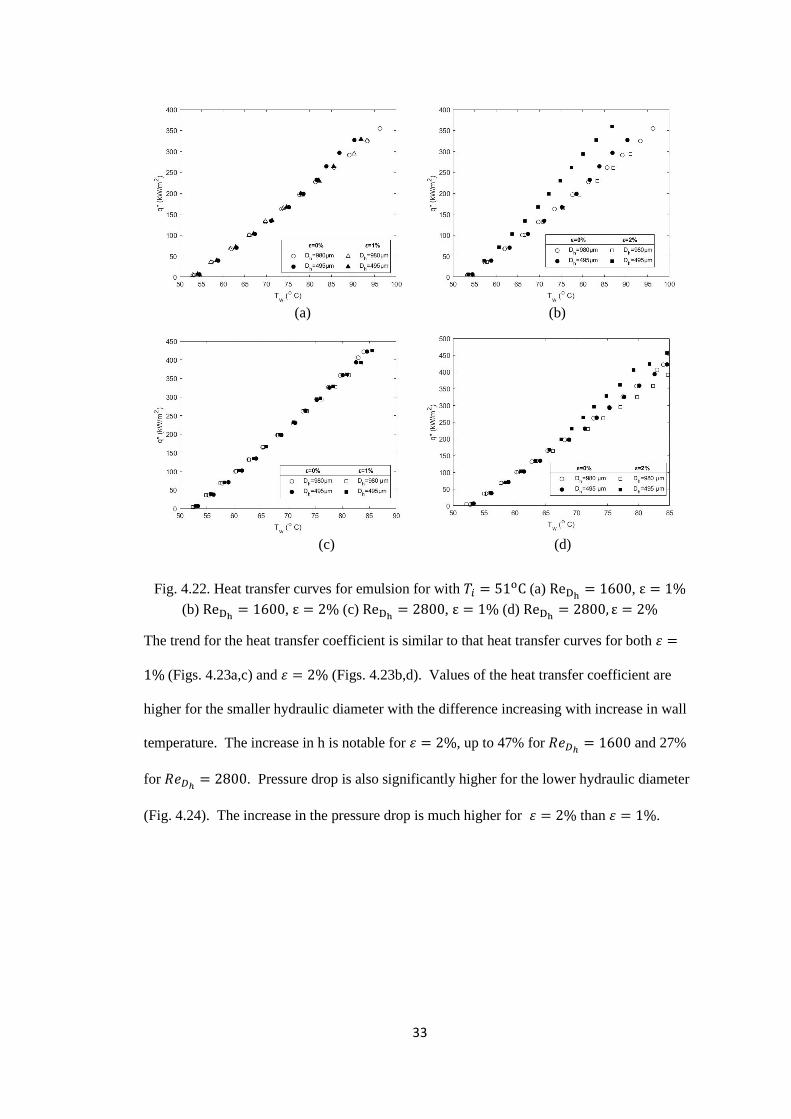
Fig. 4.22. Heat transfer curves for emulsion for with 𝑇𝑖 = 51oC (a) ReDh= 1600, ε = 1%
(b) ReDh= 1600, ε = 2% (c) ReDh
= 2800, ε = 1% (d) ReDh= 2800, ε = 2%
The trend for the heat transfer coefficient is similar to that heat transfer curves for both 휀 =
1% (Figs. 4.23a,c) and 휀 = 2% (Figs. 4.23b,d). Values of the heat transfer coefficient are
higher for the smaller hydraulic diameter with the difference increasing with increase in wall
temperature. The increase in h is notable for 휀 = 2%, up to 47% for 𝑅𝑒𝐷ℎ= 1600 and 27%
for 𝑅𝑒𝐷ℎ= 2800. Pressure drop is also significantly higher for the lower hydraulic diameter
(Fig. 4.24). The increase in the pressure drop is much higher for 휀 = 2% than 휀 = 1%.

34
(a) (b)
(c) (d)
Fig. 4.23. Heat transfer coefficient curves for emulsion for with 𝑇𝑖 = 51𝑜𝐶 (a) ReDh= 1600,
ε = 1% (b) ReDh= 1600, ε = 2% (c) ReDh
= 2800, ε = 1% (d) ReDh= 2800, ε = 2%
(a) (b)
35
(c) (d)
Fig 4.24 Heat transfer coefficient curves for emulsion for with 𝑇𝑖 = 51𝑜𝐶 (a) ReDh= 1600,
ε = 1% (b) ReDh= 1600, ε = 2% (c) ReDh
= 2800, ε = 1% (d) ReDh= 2800, ε = 2%
Shadakofsky [18] provides empirical correlation for heat transfer coefficient,
ℎ = 0.0067
𝑘𝑑
𝐷ℎ (
1
1+ε )3.42
(𝑑
𝐷ℎ)−2.37
(𝐺𝐷ℎ
𝜇𝑐)−1.48
(𝑞′′
𝐺 ℎ𝑓𝑔𝑑
)0.84
(𝐺𝐶𝑝𝑑
𝑘𝑑)2.24
(4.4)
Figure 4.25 shows the comparison between the experimental data collected in this study and
Eqn. 4.4. The data does not match with the correlation provided, less than 7% of data falls
within ±10% of the predicted value. The experimental setup for both the experiments are the
same but the correlation was developed for laminar range and 𝑇𝑖 = 30𝑜𝐶 , and the large
discrepancy can be explained based on these two factor. It is essential to take create new
correlations for the data set created in this experiment.
Fig 4.25 . Comparison between the predicted heat transfer coefficient(line) (Eqn 4.4)
and the measured values(circles).

36
5. Correlations
Based on the physical mechanisms of boiling, previous studies [18] suggest several
physical quantities that can be used to create correlations for the data
𝑘𝑑 , ⅆ , 𝐷ℎ , 𝜇𝑐 ,𝜌𝑐
𝜌𝑑, 𝐺, ℎ𝑓𝑔𝑑
, 𝐶𝑝𝑐, ε, q′′, ℎ. Based on these quantities, seven nondimensional
numbers can be constructed:
ℎ𝐷ℎ
𝑘𝑑
𝐺𝐷ℎ
𝜇𝑐
𝑞′′
𝐺ℎ𝑓𝑔𝑑
1
1 + ε
𝜌𝑑
𝜌𝑐
𝐺𝐶𝑝ⅆ
𝑘𝑑
ⅆ
𝐷ℎ
(5.1)
The first term is equivalent of Nusselt number, but the thermal conductivity of the
dispersed phase is considered instead of the mixture properties. The second term, Reynolds
number is a common parameter considered when dealing with convection data . The third
term is boiling number for the dispersed component, this would capture the effect of nucleate
boiling of the dispersed component. Fourth term accounts for the emulsion concentration.
The density ratio is an important quantity as it will decide the quantity of dispersed phase
coming in contact with heated surface, but this cannot be accounted for in this study as the
same two fluids are used in the emulsion. The sixth term accounts for the sensible heat
transfer to the continuous component. The last term accounts for the droplet size of the
dispersed phase. The droplet size is affecting the temperature overshoot beyond the
saturation temperature required for onset of nucleate boiling of the dispersed phase.
Correlation between these parameters is given by,
ℎ =
𝑘𝑑
𝐷ℎ(
1
1 + ε )−2.90
(ⅆ
𝐷ℎ)0.52
(𝐺𝐷ℎ
𝜇𝑐)2.12
(𝑞′′
𝐺ℎ𝑓𝑔𝑑
)
0.40
(𝐺𝐶𝑝ⅆ
𝑘𝑑)
−1.04
(5.2)
The correlation is a good fit with the experimental data with 93.8% of data lying between
±30% of the predicted value. Figure 5.1 shows the spread of measured data against predicted
values. Almost all the values have significant correlation based on the p-values obtained for
the variables. Table 5.1 shows the p-value for all the nondimensional numbers.

37
Fig 5.1 Comparison between the measured emulsion heat transfer coefficient and that
predicted by Eqn. (5.2). The solid line represents equivalence between the measured and
predicted values. The dashed line represents ±30% variation from the predicted value.
Table 5.1 p-values for the nondimensional quantities involved in (Eqn 5.2)
The correlation fits the experimental data but should be used cautiously for design as some of
the data points are limited for droplet diameter, hydraulic diameter and Reynolds number.
Nondimensional quantity p-value 1
1 + ε
0.071
ⅆ
𝐷ℎ
6.33e-07
𝐺𝐷ℎ
𝜇𝑐
2.46e-27
𝑞′′
𝐺ℎ𝑓𝑔𝑑
1.44e-71
𝐺𝐶𝑝ⅆ
𝑘𝑑
1.79e-15
38
6. Conclusions.
This study provides conclusions for water and dilute FC72-in-water emulsions on
smooth surfaces. The single-phase heat transfer coefficient for water increases with
increasing Reynolds number and decreasing gap size. The effect of these two parameters are
seen in Fig. 4.15, the Nusselt number varies linearly with 𝑅𝑒𝐷ℎ. 𝑃𝑟.
𝐷ℎ
𝐿. This also includes
data from [18].
The emulsion heat transfer on the smooth surfaces, value of h increases only for
volume fraction of 2% under certain conditions. Reducing the concentration to 1% provides
no additional benefit and decreases heat transfer coefficient for all gap sizes and Reynolds
number. The 2% emulsion has h higher than water for lower hydraulic diameter and higher
Reynold number. The emulsion improves heat transfer compared to water for higher
Reynolds number, lower gap sizes and higher concentrations of emulsion. Heat transfer
coefficient increases with increasing wall temperature and plateaus as higher wall
temperatures. There is significant increase in pressure drop for the emulsion with 2% volume
fraction with increasing wall temperature. Based on these observations and previously
suggested heat transfer mechanism, follow mechanisms are posited. Conduction in thin film
of FC-72 which reduces the heat transfer due to lower conductivity of FC-72, enhanced
mixing due to boiling of FC-72 which increases heat transfer and the boiling further
increasing the turbulence, enhancing the convection of the flow.
Based on previous studies and observations in this study, seven non-dimensional
constants are used to create correlations for heat transfer coefficient. A strong dependence on
all these parameters can be inferred from the low p-values. Nusselt, Reynolds and Boiling
numbers based on properties from either the dispersed or continuous phase. Other parameters
corresponded with the concentration emulsion, droplet diameter and the hydraulic diameters.
The last parameters 𝐺𝐶𝑝𝑑
𝑘𝑑 accounts for the sensible heat advected away by the dispersed phase
in comparison with the heat conducted by the dispersed phase. This accounts for the non-
boiling heat transfer of emulsion.

39
Equation 5.2 provides a good correlation for h based on the parameters discussed.
Around 93.8% data of falls within ±30% of the predicted value. No comparison can be
provided for this correlation with other studies, as there are no studies done in turbulent
regime. This correlation can be used for comparison in further studies performed for
emulsions in transition and turbulent regimes.
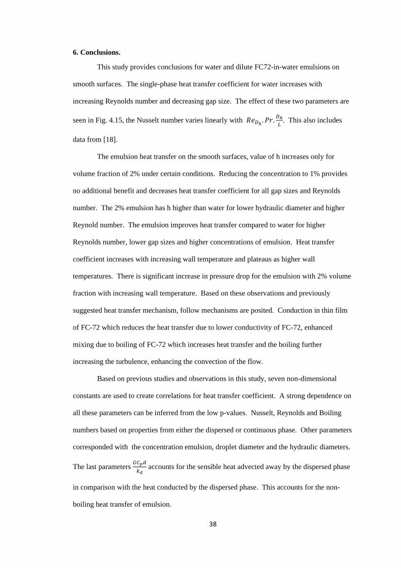
Figures 6.1 and 6.2 show the comparison of heat transfer between the emulsions and
water. For the 1% emulsion, the value of h is lower than water for all the experimental
conditions. For the 2% emulsion, the value of h is higher than water for 𝐷ℎ = 495𝜇𝑚 for all
Reynolds numbers and is lower than water for 𝐷ℎ = 980𝜇𝑚. The trends for variation of the
ratio ℎ−ℎ0
ℎ0 with hydraulic diameter is opposite to what was observed in [18], the ratio
decreases with increase in the hydraulic diameter. The ratio ℎ−ℎ0
ℎ0 increases with increase in
Reynolds number. This suggests that higher Reynolds number prevents the formation of
FC72 film on the heat transfer surface.
This study pushes the existing data set into the turbulence regime for the smooth
surfaces for a variety of conditions. Figure 6.3 shows the map of current data set available for
flow boiling in microchannels. All the previous studies have been in low Reynold number
regimes. From the observed trends, further experiments for turbulent flow boiling for
emulsions should be done for lower gap heights, higher volume fractions and higher Reynold
numbers. Further studies should be done in understanding the flow boiling of emulsion into
the following topics:
• Study droplet-droplet and droplet-wall interaction in turbulent flow should be done.
• Micro Particle image velocimetry should be used for quantifying the turbulence in the
flow.
• Develop new CFD models for flow boiling of dilute emulsion
• Trying to study the effect of droplet diameter by using monodisperse emulsions and
see the effect of droplet size on turbulence of the flow.

40
(a)
(b)
Fig. 6.1 Ratio of change in heat transfer coefficient to that for water for 𝑅𝑒𝐷ℎ= 1600 on
smooth surface. (a)-(b) are 𝐷ℎ = 495µ𝑚 and 980µ𝑚 respectively

41
(a)
(b)
Fig. 6.2 Ratio of change in heat transfer coefficient to that for water for 𝑅𝑒𝐷ℎ= 2800 on
smooth surface. (a)-(b) are 𝐷ℎ = 495µ𝑚 and 980µ𝑚 respectively

42
Waikar, Kulacki, FC-72-in-Water Janssen, Kulacki, Pentane-in-Water [17]
Janssen, Kulacki, FC72-in-Water [17] Shadakofsky, Kulacki, FC-72-in-Water [18]
Fig 6.3. Map of current data sets for flow boiling of emulsions.
43
Waikar, Kulacki,1% FC-72-in-Water Waikar, Kulacki,2% FC-72-in-Water
Janssen, Kulacki,0.1% FC72-in-Water [17] Janssen, Kulacki, 1% FC72-in-Water [17]
Janssen, Kulacki, 2% FC72-in-Water [17]
Shadakofsky, Kulacki, 0.1% FC-72-in-Water [18]
Shadakofsky, Kulacki, 0.5% FC-72-in-Water [18]
Shadakofsky, Kulacki, 1% FC-72-in-Water [18]
Shadakofsky, Kulacki, 2% FC-72-in-Water [18]
Fig. 6.4 Ratio of change in heat transfer coefficient to that for water for this study, [17] and
[18]

44
References
[1] Shah, R.K. and London, A.L. (1978) Laminar Flow Forced Convection in Ducts.
Supplement 1 to Advances in Heat Transfer. Academic Press, NY.
[2] F. Peng, G.P. Peterson, B.X. Wang, Frictional flow characteristic of water flowing
through rectangular microchannels, Experimental Heat Transfer 7 (1994)
[3] D. Pfund, D. Rector, A. Shekarriz, Pressure drop measurements in a microchannel, Fluid
Mechanics and Transport Phenomena 46 (8) (2000).
[4] Li, H., Ewoldt, R., Olsen, M.G., 2005. Turbulent and transitional velocity measurements
in a rectangular microchannel using microscopic particle image velocimetry. Experimental
Thermal and Fluid Science
[5] Li, H., Olsen,M.G., 2005 Aspect Ratio Effects on Turbulent and Transitional Flow in
Rectangular Microchannels as Measured With MicroPIV. Journal of Fluids Engineering
ASME
[7] Collier, J.G., Thome, J.R., Convective Boiling and Condensation (3rd ed. ), Oxford:
Oxford University Press, (1994).
[8] Harirchian, Tannaz and Garimella, S V., "Effects of Channel Dimension, Heat Flux, and
Mass Flux on Flow Boiling Regimes in Microchannels" (2009). CTRC Research
Publications.
[9] Mori, Y.H., Inui, E., Komotori, K., "Pool Boiling Heat Transfer to Emulsions," J. Heat
Trans., 100, pp. 613-617, (1978)
[10] Roesle, M.L., Kulacki, F.A., "An experimental study of boiling in dilute emulsions, part
A: Heat Transfer," Int. J. Heat Mass Tran., (2012).
[11] B.M. Shadakofsky, F.A. Kulacki, Boiling of dilute emulsions. Mechanisms and
applications International Journal of Heat and Mass Transfer (2019)
[12] Bulanov, N.V., Skripov, V.P., Khmyl'nin, V.A., "Heat Transfer to Emulsion with
Superheating of its Disperse Phase," J. Eng. Phys. Thermophys., 46(1), (1984).

45
[13] Gasanov, B.M., Bulanov, N.V., Baidakov, V.G., "Boiling Characteristics of Emulsions
with a Low-Boiling Dispersed Phase and Surfactants," J. Eng. Phys. Thermophys., 70(2),
(1997).
[14] Bulanov, N.V., Gasanov, B.M., "Special Features of Boiling of Emulsions with a Low-
Boiling Dispersed Phase," Heat Trans. Res., 38(3), (2007).
[15] Gasanov, B.M., Bulanov, N.V., "Effect of the Concentration and Size of Droplets of the
Dispersed Phase of an Emulsion on the Character of Heat Exchange in a Boiling Emulsion,"
High Temp., 52(1), (2014).
[16] Roesle, M.L., Kulacki, F.A., "Characteristics of two-component two-phase flow and heat
transfer in a flat microchannel," Proceedings of the ASME Summer Heat Transfer
Conference,
[17] Janssen, D., Kulacki, F.A., "Flow boiling of dilute emulsions," Int. J. Heat Mass Trans.
[18] B.M. Shadakofsky, Flow Boiling of a Dilute Emulsion on a Microporous Surface, Thesis
University of Minnesota (2018)
[19] Satish G. Kandlikar, Srinivas Garimella, Dongqing Li, Stéphane Colin and Michael R.
King , Heat Transfer and Fluid Flow in Minichannels and Microchannels, Elsevier Ltd.
Chapter 3 (2006),
[20] Kundu, Pijush K., Ira M. Cohen, and Howard H. Hu. (2004.) Fluid mechanics.

46
Appendices
A. Experimental Apparatus Drawings
Following pages contain the drawing for the experimental setup that are reproduced
form [18].
Fig. A1. Flow test section assembly.
Fig. A2. 250 𝜇𝑚 gap height top.

47
Fig. A3. 500 𝜇𝑚 gap height top.
Fig. A4. Flow test section base.
48
Fig. A5. Copper plate (Plain Surface).
Fig. A6. Garolite Heater Box.

49
B. One dimensional resistance model for heat loss
Fig. B1. Schematic diagram for resistance network for test section with 𝐷ℎ = 495 𝜇𝑚.
This section deals with estimating the heat loss from the test section. The heater
provides heat to the fluid but some of the heat is lost to the surrounding through two
mechanisms, heat conduction through the walls of the microgap and convection of heat to
surrounding from the outer surfaces of the wall. The conduction of heat in the wall can be
two-dimensional or three-dimensional but the it can be posited that the low heat conductivity
of Garolite and bigger length scales in the transverse and axial would render only one-
dimensional conduction heat transfer in wall-normal direction important. Therefore, a one-
dimensional resistance network in created for the 495𝜇𝑚 (Fig. B1) and 980𝜇𝑚 (Fig B2).
The hot fluid loses heat to the bottom and top wall through conduction and
convection from the outer surfaces. We have six different resistances in the resistance
network to account for the heat loss from the fluid.
50
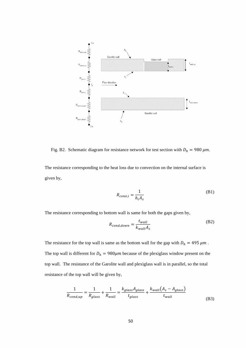
Fig. B2. Schematic diagram for resistance network for test section with 𝐷ℎ = 980 𝜇𝑚.
The resistance corresponding to the heat loss due to convection on the internal surface is
given by,
𝑅𝑐𝑜𝑛𝑣,𝑖 =
1
ℎ𝑖𝐴𝑠
(B1)
The resistance corresponding to bottom wall is same for both the gaps given by,
𝑅𝑐𝑜𝑛𝑑,𝑑𝑜𝑤𝑛 =
𝑡𝑤𝑎𝑙𝑙
𝑘𝑤𝑎𝑙𝑙𝐴𝑠
(B2)
The resistance for the top wall is same as the bottom wall for the gap with 𝐷ℎ = 495 𝜇𝑚 .
The top wall is different for 𝐷ℎ = 980𝜇𝑚 because of the plexiglass window present on the
top wall. The resistance of the Garolite wall and plexiglass wall is in parallel, so the total
resistance of the top wall will be given by,
1
𝑅𝑐𝑜𝑛𝑑,𝑢𝑝=
1
𝑅𝑔𝑙𝑎𝑠𝑠+
1
𝑅𝑤𝑎𝑙𝑙=
𝑘𝑔𝑙𝑎𝑠𝑠𝐴𝑔𝑙𝑎𝑠𝑠
𝑡𝑔𝑙𝑎𝑠𝑠+
𝑘𝑤𝑎𝑙𝑙(𝐴𝑠 − 𝐴𝑔𝑙𝑎𝑠𝑠)
𝑡𝑤𝑎𝑙𝑙
(B3)

51
The resistance provided by the convection given by the top and bottom faces is given by,
𝑅𝑐𝑜𝑛𝑣,𝑢𝑝 =
1
ℎ𝑜,𝑢𝑝𝐴𝑠
(B4)
𝑅𝑐𝑜𝑛𝑣,𝑑𝑜𝑤𝑛 =
1
ℎ𝑜,𝑑𝑜𝑤𝑛𝐴𝑠
(B5)
The values of ℎ𝑜,𝑢𝑝 and ℎ𝑜,𝑑𝑜𝑤𝑛 can be calculated using natural convection heat transfer
coefficient at the ambient temperature for upward facing and downward facing surfaces
respectively. The equivalent resistance is same for both top and bottom wall for 𝐷ℎ =
495𝜇𝑚 and is given by,
𝑅𝑒𝑞,𝑑𝑜𝑤𝑛 = 𝑅𝑖 + 𝑅𝑐𝑜𝑛𝑑,𝑑𝑜𝑤𝑛 + 𝑅𝑜,𝑑𝑜𝑤𝑛 (B6)
𝑞𝑙𝑜𝑠𝑠,𝑑𝑜𝑤𝑛=
𝑇𝑓 − 𝑇∞
𝑅𝑒𝑞,𝑑𝑜𝑤𝑛
(B7)
Heat loss through the top surface is given by similar formula and will be the same for
𝐷ℎ = 495𝜇𝑚,
𝑅𝑒𝑞,𝑢𝑝 = 𝑅𝑖 + 𝑅𝑐𝑜𝑛𝑑,𝑢𝑝 + 𝑅𝑜,𝑢𝑝 (B8)
𝑞𝑙𝑜𝑠𝑠 = 𝑞𝑙𝑜𝑠𝑠,𝑑𝑜𝑤𝑛 + 𝑞𝑙𝑜𝑠𝑠,𝑢𝑝 (B9)
To increase confidence in the estimation of heat loss, heat loss is calculated by
another approach and compared with the values given by (Eqn. B9). A control volume
approach is taken to calculate the total heat loss. Figure B3 shows control volume used for
the heat loss analysis. Energy per unit area conservation on the control volume gives,
�̇�𝑖𝑛 + �̇�𝑔𝑒𝑛 = �̇�𝑜𝑢𝑡 (B10)
�̇�𝑖𝑛 = 𝐺𝐶𝑝𝑇𝑖𝑛 (B11)
�̇�𝑜𝑢𝑡 = 𝑞𝑙𝑜𝑠𝑠 + 𝐺𝐶𝑝𝑇𝑜𝑢𝑡 (B12)
�̇�𝑔𝑒𝑛 = 𝑞′′ (B13)
𝑞′′𝑙𝑜𝑠𝑠 = 𝑞′′ − 𝐺𝐶𝑝(𝑇𝑜𝑢𝑡 − 𝑇𝑖𝑛) (B14)

52
Fig. B3. Schematic diagram for control volume around test section.
where 𝑇𝑖𝑛 and 𝑇𝑜𝑢𝑡 are inlet and outlet temperature respectively and are measured using
thermocouples. The values given by Eqn. B9 and B14 are similar to each other and thus we
can use the one-dimensional resistance network for estimating the heat loss.

53
C. Analytical Solution
Fig. C1 Microchannel Geometry
For laminar, steady, incompressible and hydrodynamically channel flow for a Newtonian
fluid with no slip wall conditions. The horizontal rectangular channel is shown in Fig. C1.
Conservation of mass and momentum is given by
𝛻 ⋅ �⃗⃗� = 0 (C1)
𝐷�⃗⃗�
𝐷𝑡= −∇(
P
𝜌) + 𝜗∇2�⃗⃗�
(C2)
Here velocity vector �⃗⃗� = (𝑢, 𝑣, 𝑤), with 𝑣 = 𝑤 = 0, the continuity equation becomes,
𝜕𝑢
𝜕𝑥= 0
(C3)
and the y and z momentum equation becomes,
𝜕𝑃
𝜕𝑦=
𝜕𝑃
𝜕𝑧= 0
(C4)
The x momentum equation becomes,
𝜕𝑃
𝜕𝑦= 𝜇(
𝜕2𝑢
𝜕𝑦2+
𝜕2𝑢
𝜕𝑧2)
(C5)
54
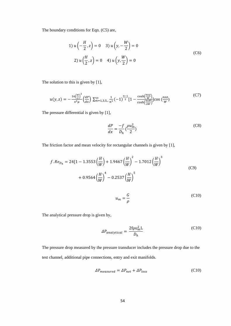
The boundary conditions for Eqn. (C5) are,
1) 𝑢 (−
𝐻
2, 𝑧) = 0 3) 𝑢 (𝑦,−
𝑊
2) = 0
2) 𝑢 (𝐻
2, 𝑧) = 0 4) 𝑢 (𝑦,
𝑊
2) = 0
(C6)
The solution to this is given by [1],
𝑢(𝑦, 𝑧) = −
16(𝑤
2)2
п3𝜇(𝑑𝑃
𝑑𝑥) ∑
1
𝑛3∞𝑛=1,3,5,.. (−1)
𝑛−1
2 [1 −cosh(
𝑛п𝑦
𝑊)
cosh(𝑛п𝐻
2𝑊)]cos (
𝑛п𝑧
𝑊)
(C7)
The pressure differential is given by [1],
ⅆ𝑃
ⅆ𝑥=
−𝑓
𝐷ℎ(𝜌𝑢𝑚
2
2)
(C8)
The friction factor and mean velocity for rectangular channels is given by [1],
𝑓. 𝑅𝑒𝐷ℎ= 24[1 − 1.3553(
𝐻
𝑊) + 1.9467(
𝐻
𝑊)2
− 1.7012(𝐻
𝑊)3
+ 0.9564(𝐻
𝑊)4
− 0.2537(𝐻
𝑊)5
(C9)
𝑢𝑚 =
𝐺
𝜌
(C10)
The analytical pressure drop is given by,
𝛥𝑃𝑎𝑛𝑎𝑙𝑦𝑡𝑖𝑐𝑎𝑙 =
2fρum2 L
𝐷ℎ
(C10)
The pressure drop measured by the pressure transducer includes the pressure drop due to the
test channel, additional pipe connections, entry and exit manifolds.
𝛥𝑃𝑚𝑒𝑎𝑠𝑢𝑟𝑒𝑑 = 𝛥𝑃𝑛𝑒𝑡 + 𝛥𝑃𝑙𝑜𝑠𝑠
(C10)
55
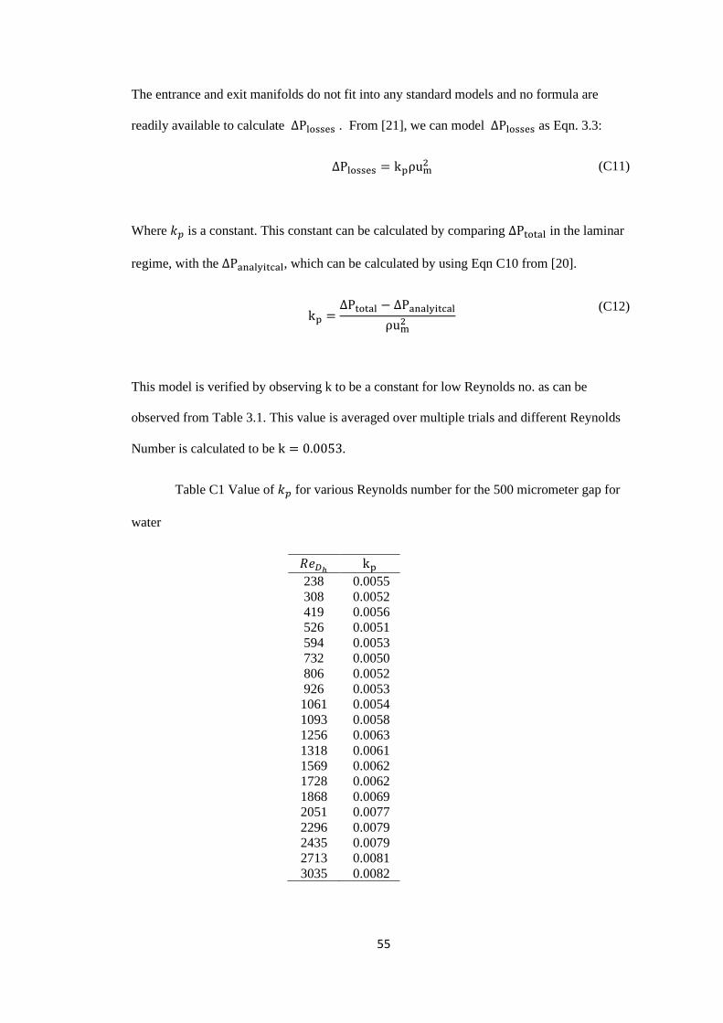
The entrance and exit manifolds do not fit into any standard models and no formula are
readily available to calculate ∆Plosses . From [21], we can model ∆Plosses as Eqn. 3.3:
∆Plosses = kpρum2
(C11)
Where 𝑘𝑝 is a constant. This constant can be calculated by comparing ∆Ptotal in the laminar
regime, with the ∆Panalyitcal, which can be calculated by using Eqn C10 from [20].
kp =
∆Ptotal − ∆Panalyitcal
ρum2
(C12)
This model is verified by observing k to be a constant for low Reynolds no. as can be
observed from Table 3.1. This value is averaged over multiple trials and different Reynolds
Number is calculated to be k = 0.0053.
Table C1 Value of 𝑘𝑝 for various Reynolds number for the 500 micrometer gap for
water
𝑅𝑒𝐷ℎ kp
238
308
419
526
594
732
806
926
1061
1093
1256
1318
1569
1728
1868
2051
2296
2435
2713
3035
0.0055
0.0052
0.0056
0.0051
0.0053
0.0050
0.0052
0.0053
0.0054
0.0058
0.0063
0.0061
0.0062
0.0062
0.0069
0.0077
0.0079
0.0079
0.0081
0.0082

56
D. Experimental data
Table D1. Experimental data for water 𝐷ℎ = 980𝜇𝑚 and 𝑇𝑖 = 51𝑜𝐶
𝑅𝑒𝐷ℎ=1600
Q (W)
𝑞𝑛𝑒𝑡′′ (𝑊𝑚2)
h (𝑊𝑚2𝐾)
∆𝑃 (kPa)
𝑇𝑤 (°𝐶)
20.55 4124.268 1123.401 10.844 53.33722 39.98 35381.44 4756.986 10.947 57.35874 59.84 67192 5891.255 10.844 61.93515 80.33 100194.6 6540.056 10.945 66.01759 99.65 131288.4 6981.465 10.948 69.72208
118.94 162310.3 7286.717 10.967 73.47 140.31 196682.7 7523.442 10.961 77.63262 159.13 227035.6 7625.804 10.973 81.31505 180.54 261465.6 7739.31 11.046 85.63936 198.91 291031.3 7848.467 11.104 89.14288
220 324914.3 7952.594 11.204 93.30716 238.6 354836 8147.977 11.35 96.24451
𝑅𝑒𝐷ℎ= 2800
Q
(W) 𝑞𝑛𝑒𝑡
′′
(𝑊
𝑚2)
h
(𝑊
𝑚2𝐾)
∆𝑃
(kPa)
𝑇𝑤
(°𝐶)
20.52 3708.349 1689.238 27.327 52.78615
40.55 35943.42 8002.345 27.33 55.31345
60.41 67905.63 9965.376 26.924 57.86314
80.36 100025.7 11058.37 27.365 60.28962
100.09 131797.9 11652.72 27.275 62.73215
120.47 164602 12056.06 27.195 65.29532
140.7 197151.5 12209.08 26.925 68.04225
180.54 261323.9 12747.4 27.445 72.71201
200.6 293576.8 12909.18 27.151 75.26158
220.6 325814.5 13126 27.256 77.44422
240.4 357694.4 13335.64 27.619 79.63538
270.2 405638.2 13623.97 27.66 82.96695
280 421467.3 13675.36 27.413 83.98048
57
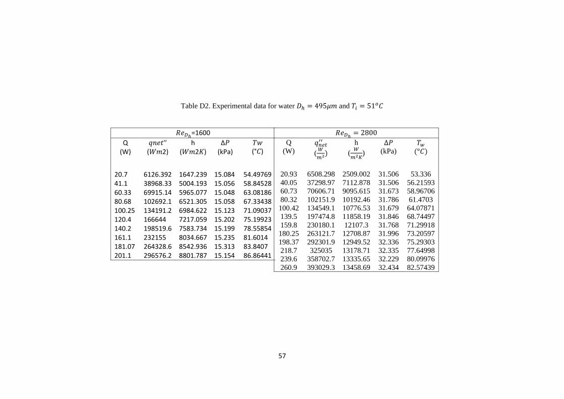
Table D2. Experimental data for water 𝐷ℎ = 495𝜇𝑚 and 𝑇𝑖 = 51𝑜𝐶
𝑅𝑒𝐷ℎ=1600
Q (W)
𝑞𝑛𝑒𝑡′′ (𝑊𝑚2)
h (𝑊𝑚2𝐾)
∆𝑃 (kPa)
𝑇𝑤 (°𝐶)
20.7 6126.392 1647.239 15.084 54.49769 41.1 38968.33 5004.193 15.056 58.84528 60.33 69915.14 5965.077 15.048 63.08186 80.68 102692.1 6521.305 15.058 67.33438 100.25 134191.2 6984.622 15.123 71.09037 120.4 166644 7217.059 15.202 75.19923 140.2 198519.6 7583.734 15.199 78.55854 161.1 232155 8034.667 15.235 81.6014 181.07 264328.6 8542.936 15.313 83.8407 201.1 296576.2 8801.787 15.154 86.86441
𝑅𝑒𝐷ℎ= 2800
Q
(W) 𝑞𝑛𝑒𝑡
′′
(𝑊
𝑚2)
h
(𝑊
𝑚2𝐾)
∆𝑃
(kPa)
𝑇𝑤
(°𝐶)
20.93 6508.298 2509.002 31.506 53.336
40.05 37298.97 7112.878 31.506 56.21593
60.73 70606.71 9095.615 31.673 58.96706
80.32 102151.9 10192.46 31.786 61.4703
100.42 134549.1 10776.53 31.679 64.07871
139.5 197474.8 11858.19 31.846 68.74497
159.8 230180.1 12107.3 31.768 71.29918
180.25 263121.7 12708.87 31.996 73.20597
198.37 292301.9 12949.52 32.336 75.29303
218.7 325035 13178.71 32.335 77.64998
239.6 358702.7 13335.65 32.229 80.09976
260.9 393029.3 13458.69 32.434 82.57439

58
Table D3. Experimental data for 휀 = 1% 𝐷ℎ = 980𝜇𝑚 and 𝑇𝑖 = 51𝑜𝐶
𝑅𝑒𝐷ℎ= 2800
Q
(W) 𝑞𝑛𝑒𝑡
′′
(𝑊
𝑚2)
h
(𝑊
𝑚2𝐾)
∆𝑃
(kPa)
𝑇𝑤
(°𝐶)
20.55 3882.875 1841.474 28.779 52.38207
40.24 35598.53 8119.01 28.68 54.81526
60.45 68124.4 9945.255 28.741 57.51081
80.29 99983.39 10773.93 28.856 60.3467
99.95 131635.9 11421.37 29.581 62.78632
120.9 165363.2 11828.19 29.529 65.45353
140.61 197126.3 11905.73 29.515 68.14939
160.44 229018 12047.41 29.186 70.88449
180.7 261623.8 12255.15 29.381 73.455
200.1 292845 12275.99 29.593 76.1857
220.6 325823.6 12462.9 29.725 78.74276
241.1 358880.1 12534.81 29.873 81.30276
260.7 390418 12789.1 29.979 83.43836
𝑅𝑒𝐷ℎ= 1600
Q
(W) 𝑞𝑛𝑒𝑡
′′
(𝑊
𝑚2)
h
(𝑊
𝑚2𝐾)
∆𝑃
(kPa)
𝑇𝑤
(°𝐶)
20.85 4748.316 1285.988 13.176 53.00632
39.95 35436.47 4744.352 13.201 57.12981
59.78 67323.81 5773.313 13.185 61.61556
80.17 100116.3 6371 13.265 65.95901
100.71 133116.7 6946.353 13.421 69.78467
120.37 164754.2 7157.388 13.586 73.87167
139.8 195934.9 7260.461 13.576 78.28709
160.18 228741.5 7453.915 13.528 82.202
200.6 293687 7728.641 13.981 90.24235
220.5 325737 7979.035 13.994 93.23515

59
Table D4. Experimental data for 휀 = 1% 𝐷ℎ = 495𝜇𝑚 and 𝑇𝑖 = 51𝑜𝐶
𝑅𝑒𝐷ℎ= 1600 𝑅𝑒𝐷ℎ
= 2800
Q
(W) 𝑞𝑛𝑒𝑡
′′
(𝑊
𝑚2)
h
(𝑊
𝑚2𝐾)
∆𝑃
(kPa)
𝑇𝑤
(°𝐶)
Q
(W) 𝑞𝑛𝑒𝑡
′′
(𝑊
𝑚2)
h
(𝑊
𝑚2𝐾)
∆𝑃
(kPa)
𝑇𝑤
(°𝐶)
20.95 6730.50 1686.08 15.96 54.0865 20.98 6623.67 2812.13 37.18 52.9792
41.43 39736.79 4798.24 16.02 58.53582 40.9 38714.07 7897.943 37.24 55.72639
61.06 71329.74 5779.749 16.006 62.89662 60.59 70427.12 9777.311 37.07 58.24943
80.6 102769.7 6371.539 16.118 67.01228 80.32 102215.1 10515.24 37.382 60.95342
100.56 134887 6719.185 16.204 71.28667 100.44 134626.5 11034.19 36.834 63.64052
120.3 166694.1 7163.3 16.151 74.65867 120.38 166773.8 11562.51 37.155 65.97996
140.6 199342.5 7621.28 16.227 77.93328 140.3 198875 11850.38 37.105 68.50259
160.28 231034.1 7682.416 16.243 82.09023 160.86 232003.8 12145.37 37.406 71.00468
180.61 263770.5 7936.824 16.197 85.50498 200.8 296368.4 12467.71 37.796 75.99857
221 328787.1 8430.576 16.377 91.84909 221 328921.3 12699.52 38.031 78.29256
240.7 360662.4 12719.11 38.114 80.92915
260.9 393210.9 12800.6 38.42 83.47112
280.3 424513 12966.02 38.444 85.52069

60
Table D5. Experimental data for 휀 = 2% 𝐷ℎ = 980𝜇𝑚 and 𝑇𝑖 = 51𝑜𝐶
𝑅𝑒𝐷ℎ= 1600 𝑅𝑒𝐷ℎ
= 2800
Q
(W) 𝑞𝑛𝑒𝑡
′′
(𝑊
𝑚2)
h
(𝑊
𝑚2𝐾)
∆𝑃
(kPa)
𝑇𝑤
(°𝐶)
Q
(W) 𝑞𝑛𝑒𝑡
′′
(𝑊
𝑚2)
h
(𝑊
𝑚2𝐾)
∆𝑃
(kPa)
𝑇𝑤
(°𝐶)
20.96 4571.903 1279.933 11.328 53.77673 20.52 3960.384 1776.481 30.332 52.18592
40.04 35285.83 4726.551 11.294 57.87073 40.8 36572.15 7765.485 30.254 54.96452
60.41 68048.12 5937.389 11.264 62.15133 60.27 67901.35 9431.408 30.249 57.69061
80.49 100332 6446.153 11.339 66.56615 80.1 99826.8 10229.46 31.442 60.4477
99.9 131533.1 6769 11.421 70.74808 101.03 133493.1 10691.22 32.592 63.4597
120.56 164735.3 6925.305 11.456 75.45966 120.09 164158.8 10978.72 33.745 66.16653
140.54 196905.8 7194.522 11.586 79.23146 140.21 196666.1 11148.92 35.076 68.76553
160.35 228773 7309.835 11.497 83.42245 160.59 229366.7 11365.21 35.914 71.7881
179.9 260194.4 7509.388 11.789 87.10426 180.24 260975.4 11636.28 36.869 74.29814
200.7 293647.1 7664.394 11.915 91.06214 201.3 294917.3 11772.17 37.685 77.04143
219.8 324677.8 11811.7 37.693 79.72136
240.5 357983.8 12008.67 37.939 82.30125
260.7 390540.2 12162.03 38.482 84.71502
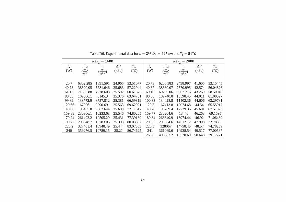
61
Table D6. Experimental data for 휀 = 2% 𝐷ℎ = 495𝜇𝑚 and 𝑇𝑖 = 51𝑜𝐶
𝑅𝑒𝐷ℎ= 1600 𝑅𝑒𝐷ℎ
= 2800
Q
(W) 𝑞𝑛𝑒𝑡
′′
(𝑊
𝑚2)
h
(𝑊
𝑚2𝐾)
∆𝑃
(kPa)
𝑇𝑤
(°𝐶)
Q
(W) 𝑞𝑛𝑒𝑡
′′
(𝑊
𝑚2)
h
(𝑊
𝑚2𝐾)
∆𝑃
(kPa)
𝑇𝑤
(°𝐶)
20.7 6302.285 1891.591 24.965 53.51077 20.73 6206.383 2498.997 41.605 53.15445
40.78 38600.05 5781.646 25.683 57.22944 40.87 38630.07 7570.995 42.574 56.04826
61.13 71366.88 7278.608 25.592 60.61875 60.16 69730.06 9367.716 43.269 58.50046
80.35 102306.1 8145.3 25.376 63.64761 80.66 102740.8 10598.45 44.011 61.00527
99.89 133772.9 8757.812 25.381 66.59819 100.33 134428.8 11402.36 44.606 63.29781
120.66 167206.1 9290.691 25.563 69.62021 120.8 167413.8 12074.68 44.54 65.55017
140.06 198405.8 9862.644 25.608 72.11617 140.28 198789.4 12729.36 45.601 67.51873
159.88 230306.1 10233.68 25.546 74.80265 159.77 230204.6 13446 46.263 69.1595
179.24 261492.2 10505.29 25.431 77.39189 180.34 263349.9 13974.44 46.92 71.06489
199.22 293648.7 10783.05 25.393 80.03832 200.3 295504.6 14512.12 47.908 72.78395
220.2 327401.4 10948.49 25.444 83.07553 220.5 328067 14758.45 48.57 74.78259
240 359276.5 10789.15 25.21 86.74625 241 361069.6 14938.54 49.517 77.00587
268.8 405882.2 15520.69 50.648 79.17221