Flow and mixing dynamics in a patterned wetland:

Kilometer-scale tracer releases in the Everglades

Evan A. Variano,1,2 David T. Ho,1,3 Victor C. Engel,4 Paul J. Schmieder,1

and Matthew C. Reid1,5

Received 12 June 2008; revised 4 April 2009; accepted 4 May 2009; published 15 August 2009.

[1] Surface water flow dynamics in the Florida Everglades were investigated using sulfurhexafluoride tracer releases, from which advection and dispersion were determined. Severalsites were studied, each characterized by different vegetation patterns and proximity tohydrologic control structures. The measured flow directions suggest that basin-scaleforcing from water management structures and operations can override the effects of locallandscape features in guiding the flow. Management effects were particularly evident intwo regions where the historic, natural landscape patterning has degraded. The large spatialscale over which tracer data were collected allows the dispersion rate to be determined atunprecedented spatial scales. These measurements showed much larger dispersioncoefficients than reported by previous experiments at smaller scales. This finding and ameasurement of the drag due to vegetation over large scales are of interest to Evergladeswater resource managers concerned with the transport of sediment and biologically activesolutes such as phosphorous.

Citation: Variano, E. A., D. T. Ho, V. C. Engel, P. J. Schmieder, and M. C. Reid (2009), Flow and mixing dynamics in a patterned

wetland: Kilometer-scale tracer releases in the Everglades, Water Resour. Res., 45, W08422, doi:10.1029/2008WR007216.

1. Introduction

[2] Advection and dispersion play an important role inwetland ecology by influencing nutrient fluxes, soil pro-cesses, and vegetation dynamics. The past century of agri-culture and urban development surrounding the FloridaEverglades has subjected this 1.5 million hectare wetlandto periodic drainage, impoundment, and/or excessive nutrientreleases [Grunwald, 2006]. These changes in hydrodynamicsand nutrient budgets have been accompanied by changes invegetative communities and wildlife habitats. Understandingthe causal links between these changes is of interest for cur-rent efforts to restore or maintain some aspects of the his-torical Everglades ecosystem.[3] A defining characteristic of the historic Everglades

was the wide expanse of shallow slow-moving oligotrophicsurface water termed sheet flow. In the areas where sheet flowoccurred, the vegetation often formed a characteristic ridgeand slough patterning, where sawgrass (Cladium jamaicense)ridges are separated by deeper water sloughs that supportsubmerged (e.g.,Utricularia spp.), floating (Nymphaea spp.)and emergent (Eleocharis spp. andPanicum spp.) vegetation.

The peat formations underlying the sawgrass ridges areslightly elevated compared to the sloughs.[4] Ridges and sloughs in the Everglades are aligned

parallel to the historic flow direction [National ResearchCouncil, 2003], and therefore sheet flow is thought to haveplayed a role in their formation [Larsen et al., 2007]. Thishypothesis is supported by observations of degraded ridgeand slough patterning in regions where the volume, timing, orvelocity of sheet flow have been disrupted. In over-drainedareas, sawgrass has expanded into the sloughs, and inimpounded areas, slough vegetation replaces sawgrass witha loss of patterning. The peat surface elevation differencesbetween the sawgrass ridges and sloughs also vary with thehydrologic setting and history of disturbance [Givnish et al.,2008].[5] Flow dynamics and vegetation populations are closely

linked in the Everglades. Vegetation creates a spatiallyvariable source of drag, thus advection and dispersion arelikely to differ between well preserved and degraded regions.Altered flow velocities, particularly in the impounded zones,are likely to affect the suspension and transport of sedimentand organicmatter that maintain ridge structure [Larsen et al.,2007]. Dispersion rates are likely sensitive to changes invegetation densities associated with altered water depths, andcan influence the rate at which excess nutrients are distributedthrough the system [Noe and Childers, 2007].[6] Dispersion associated with pipe, open channel, and

groundwater flows can be quantified using stochastic models[Taylor, 1954; Fischer et al., 1979; Gelhar, 1993]. In wet-lands, such modeling efforts are complicated by the lack ofdata on the diffusion rates and spatial variation of velocityfields that cause dispersion.Nepf et al. [1997a] collected suchdata using laboratory measurements in model wetlands, fromwhich they derived a wetland dispersion model. This model

1Lamont-Doherty Earth Observatory, Earth Institute at ColumbiaUniversity, Palisades, New York, USA.

2Now at Department of Civil and Environmental Engineering, Universityof California, Berkeley, California, USA.

3Now at Department of Oceanography, University of Hawai‘i at Manoa,Honolulu, Hawaii, USA.

4South Florida Natural Resources Center, Everglades National Park,Homestead, Florida, USA.

5Now at Department of Civil and Environmental Engineering, PrincetonUniversity, Princeton, New Jersey, USA.

Copyright 2009 by the American Geophysical Union.0043-1397/09/2008WR007216$09.00

W08422

WATER RESOURCES RESEARCH, VOL. 45, W08422, doi:10.1029/2008WR007216, 2009ClickHere

for

FullArticle

1 of 11

applies to flows with higher Reynolds number than thosetypically found in the Everglades. Detailed velocity measure-ments in the Everglades by Harvey et al. [2009] promise toyield similar advances in the creation of dispersion modelsapplicable to slow-flowing and patterned wetlands. In theabsence of such models, dispersion in the Everglades hasbeen measured directly with tracer releases [Saiers et al.,2003; Harvey et al., 2005; Dierberg et al., 2005].[7] Tracer releases in wetlands and other systems have

shown that the dispersion coefficient can increase with time,even under steady and homogeneous conditions [Fischeret al., 1979; Sabol and Nordin, 1978; Young and Jones,1991]. Such ‘‘anomalous dispersion’’ occurs when the his-tory of velocities experienced by any given tracer particle isnot an accurate representation of the spatiotemporal velocitydistribution of the flow. This can happen if too little time haspassed for the Fickian limit to be reached. Alternately,anomalous dispersion occurs when a growing plume encom-passes regions of successively greater velocity variance.When present, such a process makes it difficult to predictdispersion rates at large scales from measurements made atsmall scales. The large-scale measurements presented hereare intended to aid in the creation of dispersion models forpatterned wetlands that build on the diffusion models of Fick,Taylor and others [Fischer et al., 1979].[8] TheEverglades TracerRelease Experiment (EverTREx),

introduced by Ho et al. [2009] and discussed here, isdesigned to measure advection and dispersion at large spatial

scales in both degraded and relatively well-preserved areas.This was accomplished with a series of sulfur hexafluoride(SF6) tracer releases at scales that included multiple sawgrassridges and sloughs. The advection and dispersion valuesderived from these data include the aggregate effect oflandscape patterning, and provide a complement to previousstudies at smaller scales [Saiers et al., 2003; Lee et al., 2004;Harvey et al., 2005; Bazante et al., 2006; Solo-Gabriele,2008; Huang et al., 2008]. To date, four EverTREx cam-paigns have been held. EverTREx 1 and 2 have been exam-ined byHo et al. [2009], including some basic calculations ofadvection and dispersion. The present contribution includesEverTREx 3 and 4, and builds on the work ofHo et al. [2009]by considering variations in hydrodynamics between well-preserved and degraded portions of the landscape, and byexamining in greater detail the dispersion processes in thepatterned landscape.

2. Study Locations

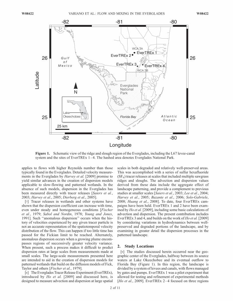
[9] The studies discussed herein occurred near the geo-graphic center of the Everglades, halfway between its sourcewaters at Lake Okeechobee and its eventual outflow toFlorida Bay (Figure 1). In this region, the landscape isdivided by a system of levees and canals, with flowsmanagedby gates and pumps. EverTREx 1 was a pilot experiment thatallowed for testing and refinement of experimental methods[Ho et al., 2009]. EverTREx 2–4 focused on three regions

Figure 1. Schematic view of the ridge and slough region of the Everglades, including the L67 levee-canalsystem and the sites of EverTREx 1–4. The hashed area denotes Everglades National Park.

2 of 11

W08422 VARIANO ET AL.: FLOW AND MIXING IN THE EVERGLADES W08422

which have been affected by the levee-canal system L67 tovarying degrees. The L67 system consists of two parallelcanal-levee pairs which route flow to the southwest, anddivide Water Conservation Area 3 (WCA 3) into WCA 3Aand 3B (Figure 1). The northern canal, L67A, is connected toother canals and is controlled at both ends by pumps andgates. The southern canal, L67C, is not connected to anyother canals or controls and thus has a more passive effect onflows. A gap exists in L67C, presenting an area of reducedresistance to flow. This gap is useful to study as a prototypefor other levee breaches proposed as part of Evergladesrestoration efforts.[10] EverTREx 2–4 were performed during wet season

conditions, summarized in Tables 1 and 2. EverTREx 2 wasperformed in WCA 3A, in a region where the landscape hasmaintained the traditional patterning [Ho et al., 2009]. Here,ridges and sloughs are O(1) km in length, and 50–500 m inwidth (Figure 2).[11] EverTREx 3 was performed in WCA 3A just north-

west of L67A, where water depths are elevated because ofimpoundment by the L67 system. The landscape there hasdistinct ridges and sloughs, but these are much smaller thanthose in traditional ridge and slough landscapes, and have awinding, sinuous shape (Figure 3).[12] EverTREx 4 was performed in WCA 3B, southeast

of the gap in L67C. Because of artificially low water levelsand short hydroperiods in this region, ridge vegetation hasgradually invaded the sloughs in WCA 3B. The remainingsloughs are small and typically aligned with the historicalflow direction (south-southeast) (Figure 4).

[13] In addition to vegetation differences, ridges andsloughs have different peat thickness that results in differentwater depths and hydrodynamics in the two community types(Table 3).Water depths weremeasured at each EverTREx siteusing a surveying staff to take three replicate depth measure-ments within a 1 m2 quadrat. Average depths were calculatedusing 20 randomly located quadrats in the ridges andsloughs. The differences in peat surface elevations werecalculated from the set of depth measurements in each ofthe two habitats. The site of EverTREx 2 displayed a sig-nificant difference between ridge and slough elevation, andin this way resembles the historic, or undisturbed, patternedlandscape (Science Coordination Team, The role of flowin the Everglades ridge and slough landscape, 2003, SouthFlorida Ecosystem Restoration Task Force, Miami, Florida,available at http://sofia.usgs.gov/publications/papers/sct_flows). The site of EverTREx 3 also displayed signifi-cant differences, albeit with greater variance. The site ofEverTREx 4 lacked clear elevation differences betweenridges and sloughs (Table 3).

3. Methods

3.1. Tracer Measurements

[14] The SF6 tracer methods were applied as described byHo et al. [2002, 2009]. For each experiment, SF6 gas wasused to saturate 8 L of water, which was then injected at thestudy site as a near-instantaneous line release that coveredthe entire depth of the water column. During the experiments,the tracer concentration field evolved because of advection,dispersion, and air-water gas exchange.

Figure 2. Selected tracer measurements from EverTREx 2. Green areas are ridges, and black or tan areasare sloughs. Each colored point represents a single tracer measurement. Blue dots are near zero con-centration and thus represent bounds to the plume’s extent. Complete tracer measurements for EverTREx 2are available in work by Ho et al. [2009].

Table 1. Locations of EverTREx Campaigns

FieldCampaign

Latitude(deg N)

Longitude(deg W) Dates

EverTREx 1 26.075180 80.711496 23 Jul to 1 Aug 2006EverTREx 2 26.034098 80.735926 29 Nov to 5 Dec 2006EverTREx 3 25.851181 80.649714 10–21 Oct 2007EverTREx 4 26.029698 80.733141 24–30 Oct 2007

Table 2. Physical Characteristics of the Study Sites

FieldCampaign

Mean Depth(cm) Landscape Pattern

EverTREx 1 31 parallel ridge and sloughEverTREx 2 42 parallel ridge and sloughEverTREx 3 75 nondirectional and fractallineEverTREx 4 46 small remnant sloughs only

W08422 VARIANO ET AL.: FLOW AND MIXING IN THE EVERGLADES

3 of 11

W08422

[15] The real-time continuous SF6 analysis system describedby Ho et al. [2002, 2009] was mounted on an airboat andused to measure the concentration of SF6 dissolved in thewater column. The detection limit was 10 fmol L�1, thus thesystem could detect SF6 concentrations that had been dilutedby a factor of O(106) relative to the initial concentrationinjected at the tracer release line. Uncertainties are discussedby Ho et al. [2009], and for the experiments presented herewere ±2% in concentration and ±5 m in position. Samplinglocations were selected on the basis of the accumulatedobservations of the evolving tracer distribution.

3.2. Vertical Structure

[16] The analyses presented here approximate the flow asvertically homogeneous. In marsh flows, the vertical velocity

profile is dominated by variations in vegetation density[Bazante et al., 2006; Leonard and Croft, 2006; Lightbodyand Nepf, 2006]. This vegetation effect overwhelms that ofthe bed and surface boundary layers, which are quite small(on the order of one vegetation diameter) even for sparsevegetation [Nepf et al., 1997a].[17] The assumption of vertical homogeneity was tested

with an acoustic Doppler current profiler (HR Profiler,NortekUSA). Measurements were made during November2007 near the tracer release location of EverTREx 4(25.901121�N, 80.565263�W), and also in a slough nearthe center of WCA 3B (25.876278�N, 80.534523�W) whichwas 4.25 km from the release location in the directionof measured flow. Average velocities (U being streamwise,V cross stream, and W vertical) were computed over 30-min

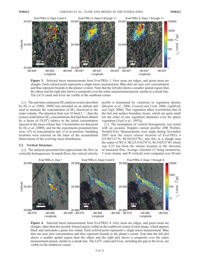
Figure 3. Selected tracer measurements from EverTREx 3. Grey areas are ridges, and green areas aresloughs. Each colored point represents a single tracer measurement. Blue dots are near zero concentrationand thus represent bounds to the plume’s extent. Note that the left plot shows a smaller spatial region thanthe others and the right plot shows a composite over the entire measurement period, similar to a streak line.The L67A canal and levee are visible in the southeast corner.

Figure 4. Selected tracer measurements from EverTREx 4. Grey areas are ridges, and green areas aresloughs, other than the recently burned region visible in the southwest corner of each image, which appearsblack and surrounds a green tree island. Each colored point represents a single tracer measurement. Bluedots are near zero concentration and thus represent bounds to the plume’s extent. Note that the left plotshows a smaller spatial region than the others and the right plot shows a composite over the entiremeasurement period, similar to a streak line. The L67C canal and levee, including the gap in the levee, arevisible in the northwest corner.

4 of 11

W08422 VARIANO ET AL.: FLOW AND MIXING IN THE EVERGLADES W08422

intervals. The velocity profiles seen in Figure 5 suggest ver-tical homogeneity in the subsection of the water column thatwas measured.[18] To ensure that the tracer data collected during

EverTREx were vertical averages, water samples were drawnfrom an intake creating a diffuse, omnidirectional poten-tial flow at middepth. In addition, vertical mixing by thermalconvection (solar heating of the peat occurs in the typicalEverglades water column which is shallow and clear) andwind shear (in locations where the water surface is not shel-tered by emergent vegetation) can lead to a vertically homo-geneous tracer distribution.

4. Results

4.1. Flow Direction

[19] Figures 2, 3, and 4 show SF6 concentrations at eachlocation sampled. The main axis of the tracer plume (foundvia a 2-D Gaussian fit, Table 4) indicates surface water flowdirection [Ho et al., 2009]. In the well-preserved landscapestudied in EverTREx 2, the overland flow measured via thetracer release was aligned with the hydraulic gradient and thelongitudinal axes of the local ridges and sloughs. In contrast,in the degraded landscape studied in EverTREx 3 and 4, theflow was not aligned with the local landscape patterning.

Instead, it was aligned with the hydraulic gradients set upby the water levels at the boundaries of WCA3 and by theinfluence of nearby control structures such as L67. Forexample, during EverTREx 3 the flow direction was alignedwith L67A, whose heading is 215�. While flowing in thissouthwesterly direction, the tracer crossed both large andsmall ridges. Similarly, in EverTREx 4 the tracer traveledthrough large expanses of sawgrass, and appeared to be unaf-fected by the presence of isolated sloughs. The flow directionduring EverTREx 4 was aligned with the direction of surfacewater flowing through the gap in the nearby L67C levee, andwith the hydraulic gradient set by the border canals.

4.2. Advection and Dispersion

[20] Advection and dispersion rates were determined fromthe data using a combination of models that were selectedon the basis of observations of the tracer distributions. Forexample, EverTREx 2 showed the long tail indicative ofanomalous diffusion (quantified by a statistically significantnegative skewness computed from a transect along the mainaxis of the plume). Therefore, the model for EverTREx 2includes processes that represent non-Fickian dispersion,while the model for EverTREx 3 and 4 uses the standardFickian dispersion term.[21] All models discussed here assume that the flow prop-

erties (including drag and dispersion rate) are spatially homo-geneous. This is justified a priori by noting that the plumeseither cross many ridges (EverTREx 3) or stay primarilywithin a single vegetation regime (EverTREx 2 and 4), thusthe landscape is essentially homogeneous at the scale of theplumes. The approximation is justified a posteriori by notingthat the models reproduce the tracer measurements well.[22] The models discussed here also assume that the flow

remains constant over the experimental time period. Thisassumption is justified by the observation of steady valuesfor key hydrodynamic forcings, namely, water depth h andhydraulic gradient (@h/@x), where the water surface eleva-tion h is defined with respect to the North American ver-tical datum (NAVD88). Gauge data from the U.S. GeologicalSurvey Everglades Depth Estimation Network (EDEN,http://sofia.usgs.gov/eden/) shows that for EverTREx 2, 3and 4, depth remained essentially constant over time. Spe-cifically, the maximum daily variation of depth at each sitewas 0.8% and the median daily variation was 0.1%. Similarly,the hydraulic gradients remained constant. During EverTREx 2the maximum daily variation in hydraulic gradient was 2.4%and the median daily variation was 1.3%. EverTREx 4showed a maximum daily variation of 4.8% and a mediandaily variation of 0.8%. The hydraulic gradients forEverTREx 2 were computed using central differences overthe 400m grid given by the EDEN daily water surface product[Ho et al., 2009]. The hydraulic gradients for EverTREx 4

Table 3. Peat Elevation Differences at the Study Sites

Field Campaign Ridge-Slough Elevation Difference (cm)

EverTREx 2 16 ± 4EverTREx 3 15 ± 13EverTREx 4 6 ± 6

Figure 5. Vertical profile of the time-averaged horizontalvelocity magnitude

ffiffiffiffiffiffiffiffiffiffiffiffiffiffiffiffiffiffiU2 þ V 2

pat two sites. Site A was near

the tracer release location for EverTREx 4, and site B was4.25 km downstream. Vertical velocities (not shown) werestatistically identical to zero. Height z � 0 at the bed, andhorizontal lines show the location of the water surface for thetwo cases. Bounding lines are the 95% confidence intervals.These data were captured by an upward looking HR Profilerresting on the peat surface; thus, the lower portion of thewater column was not measured.

Table 4. Angles of Measured Flow Direction and Local Landscape

Patterna

Field Campaign Tracer Heading (deg) Landscape Orientation (deg)

EverTREx 2 147 ± 6 150EverTREx 3 214 ± 1 169EverTREx 4 131 ± 2 167

aAngles are north � 0�, east � 90�. The value for EverTREx 3 is basedon a nearby tree island that has not lost its historical structure.

W08422 VARIANO ET AL.: FLOW AND MIXING IN THE EVERGLADES

5 of 11

W08422

were calculated from three gauges bounding the experimentalsite. Because EverTREx 3 was located near the L67 canalwhich divides the region into different hydrologic basins,the hydraulic gradient could not be measured using thesemethods, though the stability of depth at the site wasconfirmed from local gauges. This stability of externalforcing during EverTREx 2–4 supports the application ofsteady advection and dispersion models.4.2.1. Model of EverTREx 2 Before the Fickian Limit[23] A transient storage model [Deans, 1963; Bencala

and Walters, 1983; Wagner and Harvey, 1997] was used todescribe the time-dependent plume growth rate and long tailobserved in EverTREx 2. In this model, the flow is separatedinto ‘‘free’’ and ‘‘trapped’’ domains, the latter having zerovelocity and the former having a mean velocity UF. Thevolume ratio of the two domains is b, and they exchangemass at a ratea. This exchange has not, by definition, reachedthe Fickian limit, and thus leads to time-dependent spreadingand non-Gaussian plume shape. The model also includes aterm that describes plume spreading due to all those pro-cesses that have reached the Fickian limit, parameterized by asteady diffusion coefficient Dx. The three parameters, a, b,and Dx, replace the need for a time-dependent dispersioncoefficient Kx. When all dispersion processes have reachedthe Fickian limit, the transient storage model simplifies to thetraditional advection-dispersion equation with a steady Kx .[24] An additional term is included in the model to account

for the tracer that is lost to air-water gas exchange. This lossterm is based on the standard gas exchange model, namely,

F ¼ kSF6DC ¼ kSF6ðCwater � a0CairÞ; ð1Þ

where F is the flux from the water to the air, kSF6 is the gastransfer velocity for SF6, Cwater is the aqueous concentrationof SF6, a0 is the Ostwald solubility, and Cair is the concen-tration of SF6 in air. At 25�C, a0 = 0.006 [Bullister et al.,2002]. Cair 7 parts per trillion (NOAA, http://www.esrl.noaa.gov/gmd/hats/). For each data set,Cwatera0Cair, thusthe approximationDCCwater is made. For EverTREx data,this approximation results in less than 1% error in kSF6.[25] The resulting model is the Storage–Advection–

Gas Exchange–Diffusion (SAGED) model. The terms onthe right-hand side of equation (2) describe each of theseeffects in order:

@CF

@t¼ aðCT � CFÞ � UF

@CF

@x� kSF6

hCF þ Dx

@2CF

@x2ð2Þ

@CT

@t¼ ab�1ðCF � CT Þ; ð3Þ

whereCF SF6 concentration in free volume;CT SF6 concentration in trapped volume;UF advection (speed) in free volume;Dx rate of Fickian diffusion;a exchange rate between free and trapped volumes;b ratio of trapped volume to free volume;

kSF6 SF6 gas transfer velocity.

This set of equations is used with Dirichlet boundary con-ditions and a Dirac delta function initial condition havingmass M0.[26] The SAGED model is presented in one spatial dimen-

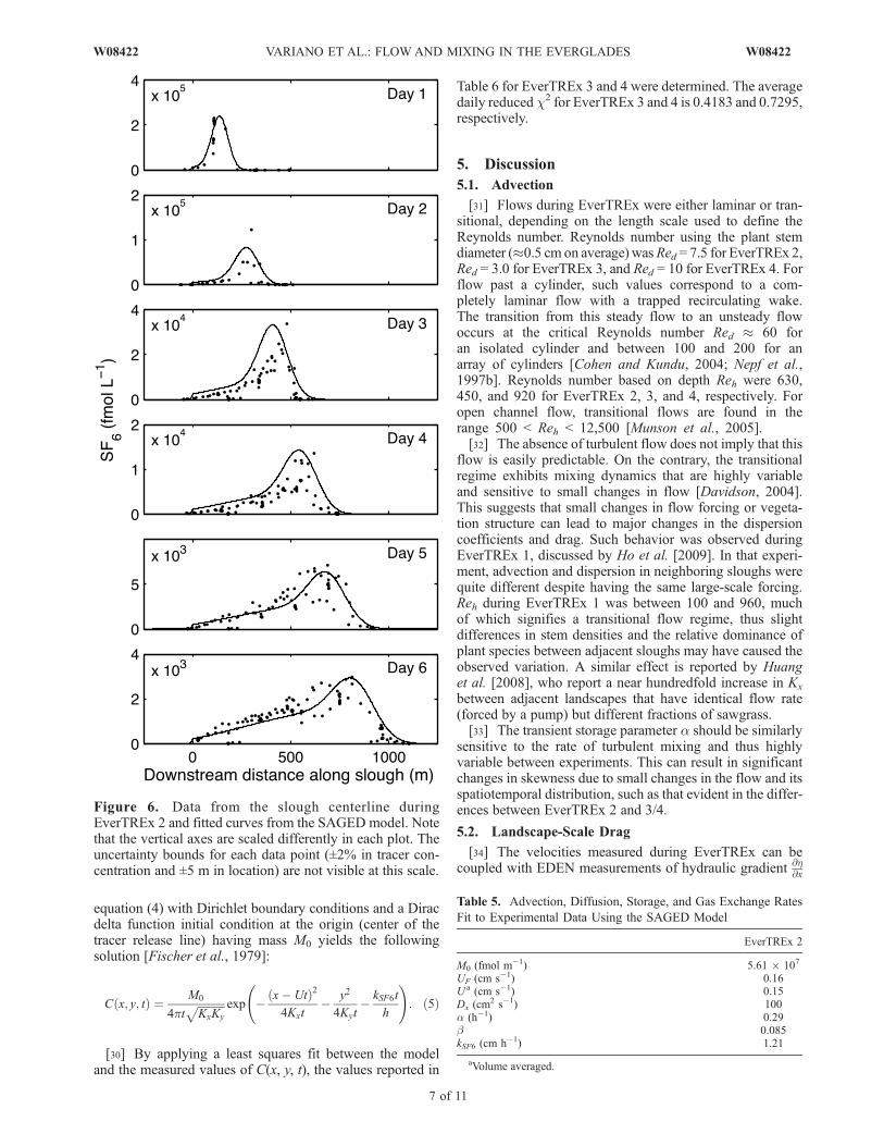
sion, which is appropriate for EverTREx 2 because therelease line was wide and perpendicular to the flow direction.Analysis is performed on the tracer data collected within±50 m of the slough centerline, where C is observed to belaterally homogeneous. The model gives a concentrationfield having many of the features typical of pre-Fickiandispersion, despite the fact that a spatially homogenous‘‘trapped’’ region is not an accurate description of the factorsthat actually cause dispersion, namely, a spatially heteroge-neous distribution of nonzero velocities correlated with vege-tation structure. Since the sampling scheme was unbiasedwith respect to these features, and since there were no inac-cessible portions of the water columnwhere the samples weretaken, the fieldmeasurements are compared to themodel usingvolume-averaged concentrations C = (CF + bCT)/(1 + b)and velocity U = UF/(1 + b).[27] Figure 6 and Table 5 show the results of the SAGED

model when it is numerically integrated and the parametersare fit to EverTREx 2 data. The reduced c2 value for the fitshown in Figure 6 is 0.7354. Model performance can also beevaluated by the Damkohler index (Da), which indicateswhether the transient storage dynamics provide a uniqueand useful extension to the traditional advection-dispersionmodel [Wagner andHarvey, 1997]. TheDamkohler index is aratio of advection time scales to storage residence time scales:Da � a (1 + b�1) L/UF, where L is the distance of down-stream transport, taken here to be 750 m. The model usedfor EverTREx 2 gives Da = 4.8, which indicates that theparameter set is unique, being of O(1) [Harvey and Wagner,2000]. Following Wagner and Harvey [1997] the value ofDa can also be used to deduce approximate uncertainties inthe transient storage parameters, which for EverTREx 2 are30% in a and 20% in b.[28] These results are complementary to the analysis per-

formed by Ho et al. [2009]. There, a Gaussian plume modelwas fit to data for each day in EverTREx 2. The Gaussianpeak showed a mean velocity over days 1–3 of 0.147 ±0.001 cm s�1 and a mean velocity over days 4–6 of 0.075 ±0.004 cm s�1. The time-dependent Kx (which includesboth the effect of Dx and transient storage) is measuredby Ho et al. [2009] to be bounded by 370 ± 140 cm2 s�1

(average over days 1–3) and 2600 ± 300 cm2 s�1 (averageover days 4–6).4.2.2. Model of EverTREx 3 and 4 at the Fickian Limit[29] Because EverTREx 3 and 4 reached the Fickian

dispersion limit rapidly, the transport model used for theseexperiments is the advectiondiffusionequation [Fischeret al.,1979]. As with the SAGED model, this model is extendedto include the effects of air-water gas exchange, giving

@C

@t¼ �UrC þKr2C � kSF6

hC: ð4Þ

If U and C are independent of z, and V =W = 0, this equationcan be simplified to two dimensions. The initial condition isa line release, but given that this line is neither perpendic-ular to the flow direction nor large compared to the plumescale, the system was modeled with a point release. Solving

6 of 11

W08422 VARIANO ET AL.: FLOW AND MIXING IN THE EVERGLADES W08422

equation (4) with Dirichlet boundary conditions and a Diracdelta function initial condition at the origin (center of thetracer release line) having mass M0 yields the followingsolution [Fischer et al., 1979]:

Cðx; y; tÞ ¼ M0

4ptffiffiffiffiffiffiffiffiffiffiKxKy

p exp �ðx� UtÞ2

4Kxt� y2

4Kyt� kSF6t

h

!: ð5Þ

[30] By applying a least squares fit between the modeland the measured values of C(x, y, t), the values reported in

Table 6 for EverTREx 3 and 4 were determined. The averagedaily reduced c2 for EverTREx 3 and 4 is 0.4183 and 0.7295,respectively.

5. Discussion

5.1. Advection

[31] Flows during EverTREx were either laminar or tran-sitional, depending on the length scale used to define theReynolds number. Reynolds number using the plant stemdiameter (0.5 cm on average) wasRed = 7.5 for EverTREx 2,Red = 3.0 for EverTREx 3, and Red = 10 for EverTREx 4. Forflow past a cylinder, such values correspond to a com-pletely laminar flow with a trapped recirculating wake.The transition from this steady flow to an unsteady flowoccurs at the critical Reynolds number Red 60 foran isolated cylinder and between 100 and 200 for anarray of cylinders [Cohen and Kundu, 2004; Nepf et al.,1997b]. Reynolds number based on depth Reh were 630,450, and 920 for EverTREx 2, 3, and 4, respectively. Foropen channel flow, transitional flows are found in therange 500 < Reh < 12,500 [Munson et al., 2005].[32] The absence of turbulent flow does not imply that this

flow is easily predictable. On the contrary, the transitionalregime exhibits mixing dynamics that are highly variableand sensitive to small changes in flow [Davidson, 2004].This suggests that small changes in flow forcing or vegeta-tion structure can lead to major changes in the dispersioncoefficients and drag. Such behavior was observed duringEverTREx 1, discussed by Ho et al. [2009]. In that experi-ment, advection and dispersion in neighboring sloughs werequite different despite having the same large-scale forcing.Reh during EverTREx 1 was between 100 and 960, muchof which signifies a transitional flow regime, thus slightdifferences in stem densities and the relative dominance ofplant species between adjacent sloughs may have caused theobserved variation. A similar effect is reported by Huanget al. [2008], who report a near hundredfold increase in Kx

between adjacent landscapes that have identical flow rate(forced by a pump) but different fractions of sawgrass.[33] The transient storage parameter a should be similarly

sensitive to the rate of turbulent mixing and thus highlyvariable between experiments. This can result in significantchanges in skewness due to small changes in the flow and itsspatiotemporal distribution, such as that evident in the differ-ences between EverTREx 2 and 3/4.

5.2. Landscape-Scale Drag

[34] The velocities measured during EverTREx can becoupled with EDEN measurements of hydraulic gradient @h

@x

Table 5. Advection, Diffusion, Storage, and Gas Exchange Rates

Fit to Experimental Data Using the SAGED Model

EverTREx 2

M0 (fmol m�1) 5.61 107

UF (cm s�1) 0.16U a (cm s�1) 0.15Dx (cm

2 s�1) 100a (h�1) 0.29b 0.085kSF6 (cm h�1) 1.21

aVolume averaged.

Figure 6. Data from the slough centerline duringEverTREx 2 and fitted curves from the SAGED model. Notethat the vertical axes are scaled differently in each plot. Theuncertainty bounds for each data point (±2% in tracer con-centration and ±5 m in location) are not visible at this scale.

W08422 VARIANO ET AL.: FLOW AND MIXING IN THE EVERGLADES

7 of 11

W08422

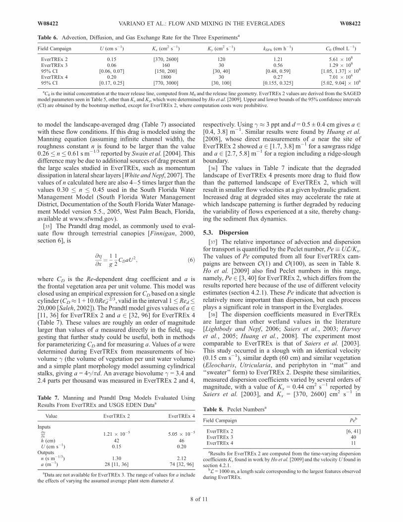
to model the landscape-averaged drag (Table 7) associatedwith these flow conditions. If this drag is modeled using theManning equation (assuming infinite channel width), theroughness constant n is found to be larger than the value0.26� n� 0.61 s m�1/3 reported by Swain et al. [2004]. Thisdifference may be due to additional sources of drag present atthe large scales studied in EverTREx, such as momentumdissipation in lateral shear layers [White and Nepf, 2007]. Thevalues of n calculated here are also 4–5 times larger than thevalues 0.30 � n � 0.45 used in the South Florida WaterManagement Model (South Florida Water ManagementDistrict, Documentation of the South Florida Water Manage-ment Model version 5.5., 2005, West Palm Beach, Florida,available at www.sfwmd.gov).[35] The Prandtl drag model, as commonly used to eval-

uate flow through terrestrial canopies [Finnigan, 2000,section 6], is

@h@x

¼ 1

g

1

2CDaU

2; ð6Þ

where CD is the Re-dependent drag coefficient and a isthe frontal vegetation area per unit volume. This model wasclosed using an empirical expression forCD based on a singlecylinder (CD 1 + 10.0Red

�2/3, valid in the interval 1�Red�20,000 [Saleh, 2002]). The Prandtl model gives values of a 2[11, 36] for EverTREx 2 and a 2 [32, 96] for EverTREx 4(Table 7). These values are roughly an order of magnitudelarger than values of a measured directly in the field, sug-gesting that further study could be useful, both in methodsfor parameterizing CD and for measuring a. Values of a weredetermined during EverTREx from measurements of bio-volume g (the volume of vegetation per unit water volume)and a simple plant morphology model assuming cylindricalstalks, giving a = 4g/pd. An average biovolume g = 3.4 and2.4 parts per thousand was measured in EverTREx 2 and 4,

respectively. Using g 3 ppt and d = 0.5 ± 0.4 cm gives a 2[0.4, 3.8] m�1. Similar results were found by Huang et al.[2008], whose direct measurements of a near the site ofEverTREx 2 showed a 2 [1.7, 3.8] m�1 for a sawgrass ridgeand a 2 [2.7, 5.8] m�1 for a region including a ridge-sloughboundary.[36] The values in Table 7 indicate that the degraded

landscape of EverTREx 4 presents more drag to fluid flowthan the patterned landscape of EverTREx 2, which willresult in smaller flow velocities at a given hydraulic gradient.Increased drag at degraded sites may accelerate the rate atwhich landscape patterning is further degraded by reducingthe variability of flows experienced at a site, thereby chang-ing the sediment flux dynamics.

5.3. Dispersion

[37] The relative importance of advection and dispersionfor transport is quantified by the Peclet number, Pe�UL/Kx.The values of Pe computed from all four EverTREx cam-paigns are between O(1) and O(100), as seen in Table 8.Ho et al. [2009] also find Peclet numbers in this range,namely, Pe 2 [3, 40] for EverTREx 2, which differs from theresults reported here because of the use of different velocityestimates (section 4.2.1). These Pe indicate that advection isrelatively more important than dispersion, but each processplays a significant role in transport in the Everglades.[38] The dispersion coefficients measured in EverTREx

are larger than other wetland values in the literature[Lightbody and Nepf, 2006; Saiers et al., 2003; Harveyet al., 2005; Huang et al., 2008]. The experiment mostcomparable to EverTREx is that of Saiers et al. [2003].This study occurred in a slough with an identical velocity(0.15 cm s�1), similar depth (60 cm) and similar vegetation(Eleocharis, Utricularia, and periphyton in ‘‘mat’’ and‘‘sweater’’ form) to EverTREx 2. Despite these similarities,measured dispersion coefficients varied by several orders ofmagnitude, with a value of Kx = 0.44 cm2 s�1 reported bySaiers et al. [2003], and Kx = [370, 2600] cm2 s�1 in

Table 6. Advection, Diffusion, and Gas Exchange Rate for the Three Experimentsa

Field Campaign U (cm s�1) Kx (cm2 s�1) Ky (cm

2 s�1) kSF6 (cm h�1) C0 (fmol L�1)

EverTREx 2 0.15 [370, 2600] 120 1.21 5.61 108

EverTREx 3 0.06 160 30 0.56 1.29 108

95% CI [0.06, 0.07] [150, 200] [30, 40] [0.48, 0.59] [1.05, 1.37] 108

EverTREx 4 0.20 1800 30 0.27 7.01 106

95% CI [0.17, 0.25] [770, 3000] [30, 100] [0.155, 0.325] [5.02, 9.04] 106

aC0 is the initial concentration at the tracer release line, computed fromM0 and the release line geometry. EverTREx 2 values are derived from the SAGEDmodel parameters seen in Table 5, other than Kx and Ky, which were determined byHo et al. [2009]. Upper and lower bounds of the 95% confidence intervals(CI) are obtained by the bootstrap method, except for EverTREx 2, where computation costs were prohibitive.

Table 7. Manning and Prandtl Drag Models Evaluated Using

Results From EverTREx and USGS EDEN Dataa

Value EverTREx 2 EverTREx 4

Inputs@h@x 1.21 10�5 5.05 10�5

h (cm) 42 46U (cm s�1) 0.15 0.20

Outputsn (s m�1/3) 1.30 2.12a (m�1) 28 [11, 36] 74 [32, 96]

aData are not available for EverTREx 3. The range of values for a includethe effects of varying the assumed average plant stem diameter d.

Table 8. Peclet Numbersa

Field Campaign Peb

EverTREx 2 [6, 41]EverTREx 3 40EverTREx 4 11

aResults for EverTREx 2 are computed from the time-varying dispersioncoefficients Kx found in work byHo et al. [2009] and the velocityU found insection 4.2.1.

bL = 1000 m, a length scale corresponding to the largest features observedduring EverTREx.

8 of 11

W08422 VARIANO ET AL.: FLOW AND MIXING IN THE EVERGLADES W08422

EverTREx 2 [Ho et al., 2009]. This difference could be par-tially explained by the highly nonlinear nature of transitionalflow (section 5.1). However, the difference in dispersion ratesis likely due primarily to the spatial scales of the respectiveexperiments. Landscape variations can cause flow hetero-geneities at scales smaller than EverTREx 2, but larger thanSaiers et al. [2003], that could explain the greater dispersionobserved in EverTREx 2.[39] Similar scale-dependent dispersion has been quanti-

fied in turbulent flows [Richardson and Stommel, 1948;Kraichnan and Montgomery, 1980] and flows through het-erogeneous porous media [Dagan, 1987; Gelhar, 1993].However, the relationship between Kx and size scale L hasnot been well quantified in wetlands. In unbounded turbulentflow,Kx has been observed to grow continuously asL4/3 overa wide range of scales, even beyond the regime where it hasbeen theoretically justified [Fischer et al., 1979]. In saturatedflow in porous media, field measurements summarized byGelhar et al. [1992] suggest that the power law growth of Kx

with L changes exponent at a critical value of L. They note,however, that the larger-scale measurements have less reli-ability. EverTREx provides a method for measuring Kx atvery large scales in wetlands, and can serve as an extremein the continuum of Kx(L). Tracer experiments at scales inbetween those of EverTREx and other existing measurementsare needed to provide a complete picture of Kx(L).[40] Ideally, both wetland dispersion and its scale depen-

dence can be derived from field-measurable landscape fea-tures. Groundwater studies have done this by making use ofthe variogram to describe spatial variations in permeability[Gelhar, 1993]. The analogy in wetlands would be a measureof the spatial autocorrelation of local drag, and the Ever-glades is an ideal system in which to perform such ananalysis. This is because the binary nature of the ridge andslough landscape makes it possible to quantify the spatialdistribution of drag using aerial images and a pair of dragvalues typical of ridges and sloughs. Combining this distri-bution with an estimate of diffusion rates allows a predictionof Kx following the theory of Taylor [Fischer et al., 1979].EverTREx data can support this analysis by providing directmeasurements of Kx as a reliable point of comparison. Alter-nately, the EverTREx data can be used to calibrate transportmodels that operate in inverse mode to derive U(x, y) fromlandscape geometry. Such a model would provide a velocityfield that is consistent with the Kx measured in EverTREx.Such results could be used with Taylor’s dispersion modelto predict diffusion rates at the EverTREx sites and values ofKx at other locations in the Everglades.[41] The ratio of longitudinal to lateral dispersion (Kx/Ky)

measured during EverTREx was also greater than thatreported by Saiers et al. [2003]. Their experiments displayeda ratio of 1, while EverTREx 2 displayed a ratio of 3 ondays 1–3 and 21.5 on days 4–6 (on average) usingvalues found by Ho et al. [2009]. Using the values found insection 4.2.2, EverTREx 3 displayed a ratio of 3 andEverTREx 4 displayed a ratio of 20. This differencebetween EverTREx and the work of Saiers et al. [2003]shows that at larger scales, the variance in u is greater thanthat in v. This suggests that the additional dispersivemechanism present at large scales increases the along-stream velocity variance more than the cross-stream velocityvariance.

5.4. Air-Water Gas Exchange Rate

[42] The gas transfer velocity kSF6 is in good agreementwith expected values. That is, it is lower than most energeticsystems, and on the order of what one sees for gently stirredflows [Garbe et al., 2007]. Most measurements and modelsfocus on the case where gas transfer is dominated by the bedboundary layer or wind forcing. These processes are likelynot the key drivers of gas transfer in the Everglades, given theslow flow velocity and the observation that surface windshear is typically quite small. For example, visual surfacesignatures during EverTREx corresponded to those expectedfor Beaufort scale values of 0 or 1 [Wright et al., 1999].[43] The gas transfer velocity shows statistically signifi-

cant differences between EverTREx 2, 3, and 4. This differ-ence may be due primarily to differences in rain between theexperiments, as enhancement of air-water gas exchange bytropical rain can be significant [Ho et al., 1997, 2000].Alternative hypotheses are motivated by the observation thatthe gas transfer velocity is less in the degraded landscapes ofEverTREx 3 and 4 than in EverTREx 2. Differences inlandscape patterning may influence gas exchange by causingdifferences in thermal convective mixing, as differentialheating of ridges and sloughs can set up horizontal thermalgradients that drive an exchange flow that enhances mixing[Nepf and Oldham, 1997; Oldham and Sturman, 2001].Another hypothesis is that different landscape patterns maycause differences in the amount of wind-sheltering andboundary layer dynamics. Studies focused directly on gastransfer would be illuminating, and would require ancillarymeasurements to investigate these dynamics.

6. Conclusions

[44] SF6 tracer releases were used to investigate thedynamics of surface water flow in a ridge and slough land-scape. Flow in a relatively intact ridge and slough habitat wasclosely aligned with the direction of landscape patterning.In contrast, flow directions in degraded landscapes followedthe influence of control structures more closely than the locallandscape patterning. Flow that is not aligned with thedirection of landscape patterning does not support the sedi-ment transport dynamics that are thought to maintain ridgeand slough patterning [Larsen et al., 2007]. Thus by alteringflow directions, control structures may accelerate the degrada-tion of patterning such as that seen at the sites of EverTREx 3and 4. This pattern loss, in turn, contributes to the loss ofhabitat conducive to wading birds and other characteristicEverglade species.[45] All three EverTREx data sets showed that both

advection and dispersion were important for determiningtransport, indicated by Peclet numbers between O(1) andO(100). Advection was such that Reynolds numbers are inthe transitional flow regime, indicating that mixing in theEverglades is sensitive to slight changes in forcing or land-scape structure. Dispersion was much larger for EverTRExthan that reported in other marsh studies, an effect whichcan be explained by the unprecedented scale of these mea-surements. This result indicates that in both degraded andnondegraded landscapes, the hydrodynamic dispersion ofsubstances such as phosphorous may occur more rapidlythan would be expected on the basis of measurements at

W08422 VARIANO ET AL.: FLOW AND MIXING IN THE EVERGLADES

9 of 11

W08422

smaller scales. Furthermore, a comparison of degraded andwell-preserved landscapes show that the vegetation in thedegraded landscape is more homogeneous and exhibits agreater drag, causing a smaller range of flow velocities in thatregion.[46] Future work using the methods of EverTREx could

be directed to further evaluate and improve models of vege-tative drag by exploring a range of flow conditions andseasonal vegetation changes at one site. Tracer releases couldalso be performed to evaluate impacts of planned restora-tion projects entailing changes in engineered flow controls.Finally, the data from EverTREx 1–4 could be used tocalibrate and validate transport models that explicitly accountfor the specific landscape features. Work of this type is cur-rently underway using Lattice-Boltzmann simulations [Sukopand Thorne, 2007].

[47] Acknowledgments. We thank Dan Childers for the use of hislaboratory, Madison Condon, Miriam Jones, Greg Losada, DamonRondeau, and Rafael Travieso for assistance in the field, and NortekUSAfor loan of the HR Profiler ADCP. We are grateful to the editor andanonymous reviewers for comments that helped improve this manuscript.Funding was provided by the National Park Service via the Critical Eco-system Studies Initiative (H5284-05-0018). EAV was funded by a post-doctoral fellowship from the National Park Service, administered by theUniversity of Florida through the Science Fellowships in EvergladesRestoration Ecology program. This is LDEO contribution 7251.

ReferencesBazante, J., G. Jacobi, H. M. Solo-Gabriele, D. Reed, S. Mitchell-Bruker,D. L. Childers, L. Leonard, and M. Ross (2006), Hydrologic measure-ments and implications for tree island formation within EvergladesNational Park, J. Hydrol., 329, 606–619.

Bencala, K. E., and R. A. Walters (1983), Simulation of solute transport in amountain pool-and-riffle stream: A transient storage model,Water Resour.Res., 19(3), 718–724.

Bullister, J. L., D. P. Wisegarver, and F. A. Menzia (2002), The solubility ofsulfur hexafluoride in water and seawater, Deep Sea Res., Part I, 49,175–187.

Cohen, I. M., and P. K. Kundu (2004), Fluid Mechanics, 3rd ed., Academic,San Diego, Calif.

Dagan, G. (1987), Theory of solute transport by groundwater, Annu. Rev.Fluid Mech., 19, 183–213.

Davidson, P. A. (2004), Turbulence: An Introduction for Scientists andEngineers, Oxford Univ. Press, New York.

Deans, H. A. (1963), A mathematical model for dispersion in the directionof flow in porous media, Trans. Soc. Pet. Eng. Am. Inst. Min. Metall. Pet.Eng., 228, 49–52.

Dierberg, F. E., J. J. Juston, T. A. DeBusk, K. Pietro, and B. Gu (2005),Relationship between hydraulic efficiency and phosphorus removal in asubmerged aquatic vegetation-dominated treatment wetland, Ecol. Eng.,25(1), 9–23.

Finnigan, J. (2000), Turbulence in plant canopies, Annu. Rev. Fluid Mech.,32, 519–571.

Fischer, H. B., J. E. List, C. R. Koh, J. Imberger, and N. H. Brooks (1979),Mixing in Inland and Coastal Waters, Academic, San Diego, Calif.

Garbe, C. S., R. A. Handler, and B. Jahne (Eds) (2007), Transport at theAir-Sea Interface: Measurements, Models and Parameterizations,Springer, Heidelberg, Germany.

Gelhar, L. W. (1993), Stochastic Subsurface Hydrology, Prentice-Hall,Englewood Cliffs, N. J.

Gelhar, L. W., C. Welty, and K. R. Rehfeldt (1992), A critical review of dataon field-scale dispersion in aquifers, Water Resour. Res., 28(7), 1955–1974.

Givnish, T. J., J. C. Volin, V. D. Owen, V. C. Volin, J. D. Muss, and P. H.Glaser (2008), Vegetation differentiation in the patterned landscape of thecentral Everglades: Importance of local and landscape drivers, GlobalEcol. Biogeogr., 17(3), 384–402.

Grunwald, M. (2006), The Swamp: The Everglades, Florida, and the Pol-itics of Paradise, Simon and Schuster, New York.

Harvey, J. W., and B. J. Wagner (2000), Quantifying hydrologic interactionsbetween streams and their subsurface hyporheic zones, in Streams andGround Waters, edited by J. B. Jones and P. J. Mulholland, pp. 3–44,Elsevier, New York.

Harvey, J. W., J. E. Saiers, and J. T. Newlin (2005), Solute transport andstorage mechanisms in wetlands of the Everglades, south Florida, WaterResour. Res., 41, W05009, doi:10.1029/2004WR003507.

Harvey, J. W., R. W. Schaffranek, G. B. Noe, L. G. Larsen, D. J. Nowacki,and B. L. O’Connor (2009), Hydroecological factors governing surfacewater flow on a low-gradient floodplain, Water Resour. Res., 45,W03421, doi:10.1029/2008WR007129.

Huang, Y. H., J. E. Saiers, J. W. Harvey, G. B. Noe, and S. Mylon (2008),Advection, dispersion, and filtration of fine particles within emergentvegetation of the Florida Everglades, Water Resour. Res., 44, W04408,doi:10.1029/2007WR006290.

Ho, D. T., L. F. Bliven, R. Wanninkhof, and P. Schlosser (1997), The effectof rain on air-water gas exchange, Tellus, Ser. B, 49(2), 149–158.

Ho, D. T., W. E. Asher, L. F. Bliven, P. Schlosser, and E. L. Gordan (2000),On mechanisms of rain-induced air-water gas exchange, J. Geophys.Res., 105(C10), 24,045–24,057.

Ho, D. T., P. Schlosser, and T. Caplow (2002), Determination of longitu-dinal dispersion coefficient and net advection in the tidal Hudson Riverwith a large-scale, high resolution SF6 tracer release experiment, Environ.Sci. Technol., 36(15), 3234–3241.

Ho, D. T., V. C. Engel, E. A. Variano, P. J. Schmieder, and M. E. Condon(2009), Tracer studies of sheet flow in the Florida Everglades, Geophys.Res. Lett., 36, L09401, doi:10.1029/2009GL037355.

Kraichnan, R. H., and D. Montgomery (1980), Two-dimensional turbu-lence, Rep. Prog. Phys., 43(5), 547–619.

Larsen, L. G., J. W. Harvey, and J. P. Crimaldi (2007), A delicate balance:Ecohydrological feedbacks governing landscape morphology in a loticpeatland, Ecol. Monogr., 77(4), 591–614.

Lee, J. K., L. C. Roig, H. L. Jenter, and H. M. Visser (2004), Drag coeffi-cients for modeling flow through emergent vegetation in the FloridaEverglades, Ecol. Eng., 22, 237–248.

Leonard, L. A., and A. L. Croft (2006), The effect of standing biomass onflow velocity and turbulence in Spartina alterniflora canopies, EstuarineCoastal Shelf Sci., 69, 325–336.

Lightbody, A. F., and H. M. Nepf (2006), Prediction of velocity profilesand longitudinal dispersion in emergent salt marsh vegetation, Limnol.Oceanogr., 51(1), 218–228.

Munson, B. R., D. Young, and T. H. Okiishi (2005), Fundamentals of FluidMechanics, 5th ed., John Wiley, New York.

National Research Council (2003), Does Water Flow Influence EvergladesLandscape Patterns?, Natl. Acad., Washington, D. C.

Nepf, H. M., and C. Oldham (1997), Exchange dynamics of a shallowcontaminated wetland, Aquat. Sci., 59(3), 193–213.

Nepf, H. M., C. G. Mugnier, and R. A. Zavistoski (1997a), The effectsof vegetation on longitudinal dispersion, Estuarine Coastal Shelf Sci., 44,675–684.

Nepf, H. M., J. A. Sullivan, and R. A. Zavistoski (1997b), A model fordiffusion within emergent vegetation, Limnol. Oceanogr., 42(8), 1735–1745.

Noe, G. B., and D. L. Childers (2007), Phosphorus budgets in Evergladeswetland ecosystems: The effects of hydrology and nutrient enrichment,Wetlands Ecol. Manage., 15(3), 189–205.

Oldham, C. E., and J. J. Sturman (2001), The effect of emergent vegetationon convective flushing in shallow wetlands: Scaling and experiments,Limnol. Oceanogr., 46(6), 1486–1493.

Richardson, L. F., and H. Stommel (1948), Note on eddy diffusion in thesea, J. Meteorol., 5(5), 238–240.

Sabol, G. V., and C. F. Nordin (1978), Dispersion in rivers as related tostorage zones, J. Hydraul. Div. Am. Soc. Civ. Eng., 104(5), 695–708.

Saiers, J. E., J. W. Harvey, and S. E. Mylon (2003), Surface-water transportof suspended matter through wetland vegetation of the Florida ever-glades, Geophys. Res. Lett., 30(19), 1987, doi:10.1029/2003GL018132.

Saleh, J. (2002), Fluid Flow Handbook, McGraw-Hill, New York.Solo-Gabriele, H. (2008), Documenting the importance of water flow toEverglades landscape structure and sediment transport in EvergladesNational Park, Agreement H500000B494 J5297050059, Univ. of Miami,Miami, Fla.

Sukop, M. C., and D. T. Thorne Jr. (2007), Lattice Boltzmann Modeling: AnIntroduction for Geoscientists and Engineers, Springer, New York.

Swain, E., M. Wolfert, J. Bales, and C. Goodwin (2004), Two-dimensionalhydrodynamic simulation of surface-water flow and transport to Florida

10 of 11

W08422 VARIANO ET AL.: FLOW AND MIXING IN THE EVERGLADES W08422

Bay through the Southern Inland and Coastal Systems (SICS), U.S. Geol.Surv. Water Resour. Invest. Rep., 03-4287, 69 pp.

Taylor, G. I. (1954), The dispersion of matter in turbulent flow through apipe, Proc. R. Soc. London, Ser. A, 223, 446–468.

Wagner, B. J., and J. W. Harvey (1997), Experimental design for estimatingparameters of rate-limited mass transfer: Analysis of stream tracer studies,Water Resour. Res., 33(7), 1731–1741.

White, B. L., and H. M. Nepf (2007), Shear instability and coherent struc-tures in shallow flow adjacent to a porous layer, J. Fluid Mech., 593,1–32.

Wright, J., E. Brown, A. Colling, D. Park, and the Open University CourseTeam (1999), Waves, Tides, and Shallow-Water Processes, ButterworthHeinemann, Milton Keynes, U. K.

Young, W. R., and S. Jones (1991), Shear dispersion, Phys. Fluids A, 3(5),1087–1101.

����������������������������V. C. Engel, South Florida Natural Resources Center, Everglades

National Park, 950 North Krome Avenue, Homestead, FL 33030, USA.

D. T. Ho, Department of Oceanography, University of Hawai‘i at Manoa,1000 Pope Road, MSB 517, Honolulu, HI 96822, USA.

M. C. Reid, Department of Civil and Environmental Engineering,Princeton University, Princeton, NJ 08544, USA.

P. J. Schmieder, Lamont-Doherty Earth Observatory, Earth Institute atColumbia University, Palisades, NY 10964, USA.

E. A. Variano, Department of Civil and Environmental Engineering,University of California, 623 Davis Hall, Berkeley, CA 94720-1710, USA.(variano@ce.berkeley.edu)

W08422 VARIANO ET AL.: FLOW AND MIXING IN THE EVERGLADES

11 of 11

W08422