Flexible Radio Resource Management for Multicast ...
167
HAL Id: tel-02084439 https://tel.archives-ouvertes.fr/tel-02084439 Submitted on 29 Mar 2019 HAL is a multi-disciplinary open access archive for the deposit and dissemination of sci- entific research documents, whether they are pub- lished or not. The documents may come from teaching and research institutions in France or abroad, or from public or private research centers. L’archive ouverte pluridisciplinaire HAL, est destinée au dépôt et à la diffusion de documents scientifiques de niveau recherche, publiés ou non, émanant des établissements d’enseignement et de recherche français ou étrangers, des laboratoires publics ou privés. Flexible Radio Resource Management for Multicast Multimedia Service Provision : Modeling and Optimization Qing Xu To cite this version: Qing Xu. Flexible Radio Resource Management for Multicast Multimedia Service Provision : Modeling and Optimization. Operations Research [cs.RO]. Université de Technologie de Belfort-Montbeliard, 2014. English. NNT : 2014BELF0237. tel-02084439
-
Upload
khangminh22 -
Category
Documents
-
view
0 -
download
0
Transcript of Flexible Radio Resource Management for Multicast ...

HAL Id: tel-02084439https://tel.archives-ouvertes.fr/tel-02084439
Submitted on 29 Mar 2019
HAL is a multi-disciplinary open accessarchive for the deposit and dissemination of sci-entific research documents, whether they are pub-lished or not. The documents may come fromteaching and research institutions in France orabroad, or from public or private research centers.
L’archive ouverte pluridisciplinaire HAL, estdestinée au dépôt et à la diffusion de documentsscientifiques de niveau recherche, publiés ou non,émanant des établissements d’enseignement et derecherche français ou étrangers, des laboratoirespublics ou privés.
Flexible Radio Resource Management for MulticastMultimedia Service Provision : Modeling and
OptimizationQing Xu
To cite this version:Qing Xu. Flexible Radio Resource Management for Multicast Multimedia Service Provision : Modelingand Optimization. Operations Research [cs.RO]. Université de Technologie de Belfort-Montbeliard,2014. English. NNT : 2014BELF0237. tel-02084439

Thèse de Doctorat
n
é c o l e d o c t o r a l e s c i e n c e s p o u r l ’ i n g é n i e u r e t m i c r o t e c h n i q u e s
U N I V E R S I T É D E T E C H N O L O G I E B E L F O R T - M O N T B É L I A R D
Flexible Radio ResourceManagement for MulticastMultimedia Service Provision:Modeling and Optimization
Qing XU


Thèse de Doctorat
é c o l e d o c t o r a l e s c i e n c e s p o u r l ’ i n g é n i e u r e t m i c r o t e c h n i q u e s
U N I V E R S I T É D E T E C H N O L O G I E B E L F O R T - M O N T B É L I A R D
THESE presentee par
Qing XUpour obtenir le
Grade de Docteur del’Universite de Technologie de Belfort-Montbeliard
Specialite : Informatique
Flexible Radio Resource Management for MulticastMultimedia Service Provision:
Modeling and Optimization
Soutenue le 29 Aout 2014 devant le Jury :
Aiqun HU Rapporteur Professeur a Southeast UniversityStuart ALLEN Rapporteur Professeur a Cardiff UniversityAbdel LISSER Examinateur Professeur a Universite Paris Sud – OrsayJin-Kao HAO Examinateur Professeur a Universite d’Angers, LERIA -
Faculte des SciencesAlexandre CAMINADA Directeur de these Professeur a l’UTBMHakim MABED Co-Directeur Maıtre de Conferences a l’Universite de
Franche-ComteFrederic LASSABE Co-Directeur Enseignant-Chercheur a l’UTBM
N˚ 2 3 7


Acknowledgments
Foremost, I would like to express my sincere gratitude to my thesis advisorProf. Dr. Alexandre CAMINADA, for his continuous support to my PhD studyand research, for his patience, motivation, enthusiasm, insightful comments andimmense knowledge. His guidance helped during the time of my research and writingof this thesis. I would like to thank my co-advisor Assoc. Prof. Dr. Hakim Mabedand Dr. Frédéric Lassabe for their professional advice, patience, encouragement andfriendship. I could not have imagined having a better group of advisors and mentorsfor my PhD study.
I would like to thank my friends who have supported me with their friendshipand encouragement all these years of my studies.
Last but certainly not least, with my love and gratitude, I want to dedicate thisPhD dissertation to my father and mother, to my husband and my son. They allsupported me generously and unconditionally throughout my studies.


Résumé
Le conflit entre la demande de services multimédia en multidiffusion à haut débit(MBMS) et les limites en ressources radio demandent une gestion efficace de l’allocationdes ressources radio (RRM) dans les réseaux 3G UMTS. À l’opposé des travaux ex-istant dans ce domaine, cette thèse se propose de résoudre le problème de RRM dansles MBMS par une approche doptimisation combinatoire. Le travail commence parune modélisation formelle du problème cible, désigné comme Flexible Radio Re-source Management Model (F2R2M). Une analyse de la complexité et du paysagede recherche est effectuée à partir de ce modèle. Tout dabord on montre qu’enassouplissant les contraintes de code OVSF, le problème de RRM pour les MBMSpeut s’apparenter à un problème de sac à dos à choix multiples (MCKP). Une telleconstatation permet de calculer les limites théoriques de la solution en résolvant leMCKP similaire. En outre, l’analyse du paysage montre que les espaces de recherchesont accidentés et constellés d’optima locaux. Sur la base de cette analyse, des al-gorithmes métaheuristiques sont étudiés pour résoudre le problème. Nous montronstout d’abord que un Greedy Local Search (GLS) et un recuit simulé (SA) peuventtrouver de meilleures solutions que les approches existantes implémentées dans lesystème UMTS, mais la multiplicité des optima locaux rend les algorithmes très in-stables. Un algorithme de recherche tabou (TS) incluant une recherche à voisinagevariable (VNS) est aussi développé et comparé aux autres algorithmes (GLS et SA)et aux approches actuelles du système UMTS; les résultats de la recherche taboudépassent toutes les autres approches. Enfin les meilleures solutions trouvées parTS sont également comparées avec les solutions théoriques générées par le solveurMCKP. On constate que les meilleures solutions trouvées par TS sont égales ou trèsproches des solutions optimales théoriques.
Mots clés: gestion des ressources radio UMTS, service multimédia MBMS, trans-mission à échelle variable, problème de sac à dos, recherche tabou et recherche àvoisinage variable.


Abstract
The high throughputs supported by the multimedia multicast services (MBMS) andthe limited radio resources result in strong requirement for efficient radio resourcemanagement (RRM) in UMTS 3G networks. This PhD thesis proposes to solve theMBMS RRM problem as a combinatorial optimization problem. The work startswith a formal modeling of the problem, named as the Flexible Radio ResourceManagement Model (F2R2M). An in-depth analysis of the problem complexity andthe search landscape is done based on this model. It is showed that, by relaxingthe OVSF code constraints, the MBMS RRM problem can be approximated as aMultiple-Choice Knapsack Problem (MCKP). Such work allows us to compute thetheoretical solution bounds by solving the approximated MCKP. Then the fitnesslandscape analysis shows that the search spaces are rough and reveal several localoptimums. Based on the analysis, some metaheuristic algorithms are studied tosolve the MBMS RRM problem. We first show that a Greedy Local Search (GLS)and a Simulated Annealing (SA) allow us to find better solutions than the existingapproaches implemented in the UMTS system, however the results are instable dueto the landscape roughness. Finally we have developed a Tabu Search (TS) mixedwith a Variable Neighborhood Search (VNS) algorithm and we have compared itwith GLS, SA and UMTS embedded algorithms. Not only the TS outperformsall the other approaches on several scenarios but also, by comparing it with thetheoretical solution bounds generated by the MCKP solver, we observe that TS isequal or close to the theoretical optimal solutions.
Keyword: UMTS radio resource management, MBMS multimedia services, scal-able transmission, knapsack problem, Tabu Search, Variable Neighborhood Search.

Contents
Introduction 1
1 Background Knowledge 5
1.1 Universal Mobile Telecommunications System . . . . . . . . . . . . . 6
1.1.1 UMTS network architecture . . . . . . . . . . . . . . . . . . . 6
1.1.2 UMTS channels . . . . . . . . . . . . . . . . . . . . . . . . . . 10
1.1.3 Wideband Code Division Multiple Access (WCDMA) . . . . . 12
1.2 Multicast in 3G and 3G+ . . . . . . . . . . . . . . . . . . . . . . . . 14
1.2.1 Multicast in UMTS network prior to MBMS . . . . . . . . . . 14
1.2.2 Multimedia Broadcast Multicast Service (MBMS) . . . . . . . 16
1.2.3 MBMS transmission modes . . . . . . . . . . . . . . . . . . . 22
1.3 High Speed Downlink Packet Access (HSDPA) . . . . . . . . . . . . 24
1.4 State of the art for MBMS RRM . . . . . . . . . . . . . . . . . . . . 25
1.4.1 MBMS UE counting . . . . . . . . . . . . . . . . . . . . . . . 25
1.4.2 MBMS power counting . . . . . . . . . . . . . . . . . . . . . . 26
1.4.3 MBMS FACH enhancements . . . . . . . . . . . . . . . . . . 26
1.4.4 Dual transmission mode . . . . . . . . . . . . . . . . . . . . . 28
1.4.5 MBMS over HSDPA . . . . . . . . . . . . . . . . . . . . . . . 28
1.4.6 Literature analysis and motivation . . . . . . . . . . . . . . . 29
1.5 Synthesis . . . . . . . . . . . . . . . . . . . . . . . . . . . . . . . . . 30
2 F2R2M: A Flexible Model for RRM of MBMS 33
2.1 Model framework . . . . . . . . . . . . . . . . . . . . . . . . . . . . . 35
Contents
2.1.1 Phase 1: Parameter collection phase . . . . . . . . . . . . . . 35
2.1.2 Phase 2: Estimation phase . . . . . . . . . . . . . . . . . . . . 37
2.1.3 Phase 3: Resource allocation phase . . . . . . . . . . . . . . . 38
2.2 Model abstraction . . . . . . . . . . . . . . . . . . . . . . . . . . . . 38
2.2.1 UE partition search engine . . . . . . . . . . . . . . . . . . . 38
2.2.2 Channel code allocator and availability control . . . . . . . . 43
2.2.3 Power emulator and feasibility control . . . . . . . . . . . . . 45
2.2.4 Solution evaluator . . . . . . . . . . . . . . . . . . . . . . . . 51
2.2.5 Model complexity . . . . . . . . . . . . . . . . . . . . . . . . . 52
2.2.6 Model synthesis . . . . . . . . . . . . . . . . . . . . . . . . . . 52
2.3 Simulation setup . . . . . . . . . . . . . . . . . . . . . . . . . . . . . 54
2.3.1 Simulation parameters . . . . . . . . . . . . . . . . . . . . . . 55
2.3.2 Simulation scenarios . . . . . . . . . . . . . . . . . . . . . . . 55
2.3.3 Power simulation of three transport channels . . . . . . . . . 56
2.4 Synthesis . . . . . . . . . . . . . . . . . . . . . . . . . . . . . . . . . 61
3 Model Analysis 65
3.1 Knapsack problem approximation . . . . . . . . . . . . . . . . . . . . 66
3.1.1 Knapsack problem and its variants . . . . . . . . . . . . . . . 66
3.1.2 Approximating MBMS RRM as a knapsack problem . . . . . 68
3.1.3 Solution bound generation of F2R2M by solving MCKP . . . 76
3.2 Fitness landscape analysis . . . . . . . . . . . . . . . . . . . . . . . . 79
3.2.1 Introduction of fitness landscape analysis . . . . . . . . . . . 80
3.2.2 Solution representations . . . . . . . . . . . . . . . . . . . . . 81
3.2.3 Distance measurements . . . . . . . . . . . . . . . . . . . . . 82

Contents
3.2.4 Greedy Local Search and its application on landscape analysis 83
3.2.5 Experiments and results analysis . . . . . . . . . . . . . . . . 83
3.3 Synthesis . . . . . . . . . . . . . . . . . . . . . . . . . . . . . . . . . 90
4 Solving MBMS RRM Problem by Simulated Annealing 95
4.1 Introduction of simulated annealing algorithm . . . . . . . . . . . . . 96
4.2 Algorithm design . . . . . . . . . . . . . . . . . . . . . . . . . . . . . 99
4.2.1 Algorithm framework . . . . . . . . . . . . . . . . . . . . . . . 99
4.2.2 Solution initialization . . . . . . . . . . . . . . . . . . . . . . 100
4.2.3 Annealing schedule . . . . . . . . . . . . . . . . . . . . . . . . 101
4.2.4 Select_flow(): flow selection . . . . . . . . . . . . . . . . . . . 101
4.2.5 Random_move(): solution generation . . . . . . . . . . . . . 103
4.2.6 Evaluation(): solution evaluation . . . . . . . . . . . . . . . . 103
4.3 Results and comparison with existing approaches . . . . . . . . . . . 105
4.4 Synthesis . . . . . . . . . . . . . . . . . . . . . . . . . . . . . . . . . 109
5 Solving MBMS RRM Problem by Tabu Search 111
5.1 Introduction of tabu search algorithm . . . . . . . . . . . . . . . . . 112
5.2 Algorithm design . . . . . . . . . . . . . . . . . . . . . . . . . . . . . 113
5.2.1 Move operator and neighborhood generation . . . . . . . . . . 115
5.2.2 Design of tabu memory structures . . . . . . . . . . . . . . . 117
5.2.3 Adaptive tabu tenure . . . . . . . . . . . . . . . . . . . . . . . 120
5.2.4 Tabu repair mechanism . . . . . . . . . . . . . . . . . . . . . 120
5.3 Experiments and results analysis . . . . . . . . . . . . . . . . . . . . 121
5.3.1 Analysis of tabu search strategies . . . . . . . . . . . . . . . . 121
5.3.2 Results comparison with other metaheuristic algorithms . . . 124

Contents
5.3.3 Performance comparison with theoretical lower bounds . . . . 127
5.4 Synthesis . . . . . . . . . . . . . . . . . . . . . . . . . . . . . . . . . 127
Conclusion and Future Work 129
A Appendix A: Acronyms 133
B Appendix B: CQI mapping table 137
Bibliography 141

List of Tables
1.1 MBMS services and potential applications . . . . . . . . . . . . . . . 19
1.2 Comparison of properties of transport channels . . . . . . . . . . . . 24
2.1 Candidate transport channel assignment . . . . . . . . . . . . . . . . 38
2.2 Single insert operation example . . . . . . . . . . . . . . . . . . . . . 41
2.3 Multiple insert operation example . . . . . . . . . . . . . . . . . . . . 42
2.4 Spreading factor and downlink user bit rate in UMTS FDD [5] . . . 44
2.5 Estimated S-CCPCH power vs. cell coverage (PedestrianB 3km/h) [5] 46
2.6 System level parameter setting . . . . . . . . . . . . . . . . . . . . . 56
2.7 Experimental scenarios . . . . . . . . . . . . . . . . . . . . . . . . . . 57
3.1 Items list in class K1 . . . . . . . . . . . . . . . . . . . . . . . . . . . 74
3.2 Simulation scenarios for MCKP based formulation . . . . . . . . . . 77
3.3 Solutions found by Gurobi . . . . . . . . . . . . . . . . . . . . . . . . 79
3.4 Distance between solutions of LSI . . . . . . . . . . . . . . . . . . . . 85
3.5 Distance between solutions of LMI . . . . . . . . . . . . . . . . . . . 86
3.6 Fitness values of Slo,SI . . . . . . . . . . . . . . . . . . . . . . . . . . 87
3.7 Fitness values of Slo,MI . . . . . . . . . . . . . . . . . . . . . . . . . 88
3.8 Step lengths of the two landscapes . . . . . . . . . . . . . . . . . . . 88
3.9 Performance of the Greedy Local Search with δSI and δMI . . . . . . 93
4.1 Values of T0 with Equation 4.2 . . . . . . . . . . . . . . . . . . . . . 102
4.2 Comparison between two flow selection methods . . . . . . . . . . . . 103
4.3 Best solutions found by different MBMS RRM algorithms . . . . . . 106

List of Tables
4.4 Detailed solutions of 3s80uSNN . . . . . . . . . . . . . . . . . . . . . 108
5.1 Move structure . . . . . . . . . . . . . . . . . . . . . . . . . . . . . . 116
5.2 A move example m1: from x1 to x2 . . . . . . . . . . . . . . . . . . . 117
5.3 Three tabu structure definitions . . . . . . . . . . . . . . . . . . . . . 119
5.4 Tabus states (type tabu-pen) based on move m1 . . . . . . . . . . . . 119
5.5 A tabu move for x5 . . . . . . . . . . . . . . . . . . . . . . . . . . . . 120
5.6 TS solutions without tabu repair mechanism . . . . . . . . . . . . . . 123
5.7 TS solutions with tabu repair mechanism . . . . . . . . . . . . . . . 123
5.8 Best solutions found by three metaheuristic algorithms . . . . . . . . 126
5.9 Average time cost (second) . . . . . . . . . . . . . . . . . . . . . . . . 126
5.10 Solution lower bounds found by Gurobi and the best solutions foundby F2R2M-TS . . . . . . . . . . . . . . . . . . . . . . . . . . . . . . . 127
B.1 CQI mapping table [13] . . . . . . . . . . . . . . . . . . . . . . . . . 137

List of Figures
1.1 UMTS network architecture . . . . . . . . . . . . . . . . . . . . . . . 6
1.2 Radio interface protocol stacks in access stratum . . . . . . . . . . . 9
1.3 Logical channel to transport channel mapping . . . . . . . . . . . . . 10
1.4 Transport channel to physical channel mapping . . . . . . . . . . . . 11
1.5 OVSF code tree used for orthogonal spreading . . . . . . . . . . . . . 12
1.6 Multicast duplication in UMTS network prior to MBMS [51] . . . . . 15
1.7 Enhancement of MBMS in UMTS [18] . . . . . . . . . . . . . . . . . 17
1.8 Multicast procedure [16] . . . . . . . . . . . . . . . . . . . . . . . . . 20
1.9 An example of two users receiving MBMS multicast service . . . . . 21
1.10 MBMS transmission modes and channel mapping . . . . . . . . . . . 23
2.1 A three phase framework . . . . . . . . . . . . . . . . . . . . . . . . . 35
2.2 Model abstraction in the estimation phase . . . . . . . . . . . . . . . 39
2.3 Allocation of spreading codes: an example . . . . . . . . . . . . . . . 45
2.4 FACH transmission power obtained by OPNET 15.0.A . . . . . . . . 47
2.5 Cellular layout in simulation setup . . . . . . . . . . . . . . . . . . . 55
2.6 Three user distributions for power comparison . . . . . . . . . . . . . 58
2.7 Separate power consumption of the three channels for 32 kbps and64 kbps services . . . . . . . . . . . . . . . . . . . . . . . . . . . . . . 59
2.8 Separate power consumption of three channels for 128 kbps and 256kbps services . . . . . . . . . . . . . . . . . . . . . . . . . . . . . . . 60
3.1 User distributions of six scenarios . . . . . . . . . . . . . . . . . . . . 84
3.2 Two fitness spaces of scenario 5 (3s100uSNN) . . . . . . . . . . . . . 86

List of Figures
3.3 Fitness distance scatter: scenarios 1, 2 . . . . . . . . . . . . . . . . . 89
3.4 Fitness distance scatter: scenarios 3, 4 . . . . . . . . . . . . . . . . . 91
3.5 Fitness distance scatter: scenarios 5, 6 . . . . . . . . . . . . . . . . . 92
5.1 Best neighborhood selection in F2R2M-TS . . . . . . . . . . . . . . . 114
5.2 Tabu repair mechanism: an example . . . . . . . . . . . . . . . . . . 120
5.3 TS strategies comparison . . . . . . . . . . . . . . . . . . . . . . . . . 122
5.4 Rank distributions of three metaheuristic algorithms . . . . . . . . . 124

List of Algorithmes
1 Lexicographic evaluation. . . . . . . . . . . . . . . . . . . . . . . . . 512 Greedy Local Search [45] . . . . . . . . . . . . . . . . . . . . . . . . . 833 General SA algorithm [36] . . . . . . . . . . . . . . . . . . . . . . . . 964 F2M2R-SA algorithm . . . . . . . . . . . . . . . . . . . . . . . . . . 995 Initialize() . . . . . . . . . . . . . . . . . . . . . . . . . . . . . . . . . 1006 Random_move() . . . . . . . . . . . . . . . . . . . . . . . . . . . . . 1047 Evaluation() . . . . . . . . . . . . . . . . . . . . . . . . . . . . . . . . 1048 General TS algorithm [44] . . . . . . . . . . . . . . . . . . . . . . . . 1129 F2R2M-TS algorithm . . . . . . . . . . . . . . . . . . . . . . . . . . . 11310 Neighborhood_generate() . . . . . . . . . . . . . . . . . . . . . . . . 118


Introduction
In the past decades, the rapid growth of mobile communication technology booststhe demand of wireless multimedia services. According to the Cisco mobile forecasthighlights [20], the global consumer mobile data traffic grew of 74% in 2012, andgrew more than 81% in 2013. From 2013 to 2018, the mobile data traffic is expectedto grow at 61% Compound Annual Growth Rate (CAGE). By 2018, 69% of theworld mobile data traffic will be video, up from 53% in 2013. The rapid growthof multimedia mobile data demands higher transmission rate with lower radio andnetwork resource cost. Hence the content and service providers are increasinglyinterested in more efficient multicast communications over mobile networks.
The Universal Mobile Telecommunications System (UMTS) is the second world’smost widely used wireless technology with 500 million customers [19]. In the ra-dio network of UMTS where the radio resources (power and channelization codes)are limited, the sharing of resources among numerous users per cell is constrainedwith more services subscriptions and higher traffic bandwidth requirements. HenceUMTS is facing challenges with the rapid growth of multicast multimedia ser-vice requirement. In order to provide an efficient multicast and broadcast trans-mission platform in mobile networks, the 3GPP specified the Multimedia Broad-cast/Multicast Service (MBMS) since Release 6 specifications [16].
In MBMS, the broadcast/multicast data are provided by a particular servicecenter which performs control functions for all individual users in the same MBMSregion. For each MBMS service, only one MBMS tunnel is established, throughwhich the service data is sent to a class D IP multicast address (identifying a mul-ticast group). Hence the network resource is saved by avoiding content duplication.In the radio air link, MBMS defines common logical channels for multicast dataand signaling transmission. The same service is served to multiple users by a acommon signal transmission facility and bearer (point-to-multipoint transmissionmode), hence conserving radio resources.
MBMS aims to provide more efficient multimedia streaming within UMTS. Sincethe radio resource is limited in UMTS, to provide the multimedia service with satis-fied quality requirement by using minimal transmission power and channel codes isthe most critical topic in MBMS study. Besides, if the point-to-multipoint carrier isused for service that are not popular, the complicated MBMS signaling will actuallylead to more overhead than with a simple unicast link. With these considerations,a wide range of work is investigated on the efficient Radio Resource Management(RRM) for MBMS. The literature in this field mainly focus on the static switchingbetween conventional MBMS transmission modes. That is because different chan-nels for carrying MBMS traffic have different characteristics in power consumption.

2 Introduction
To bring additional gains, the enhancement in physical layer such as Macro Diversityand Spatio-Temporal Transmit Diversity (STTD) are also proposed. Few studiesmention the selection of transmitted content for multicast service, which is basedon the scalability encoding technology. Besides, stream schedule is another topic inthe field of MBMS RRM, the base station needs to schedule streams by determiningthe target multicast group and transmit rate per time slot.
By emphasizing the existing literatures, some shortcomings are identified: first,the approaches are mono-objective, e.g. only consider the power consumption. Inaddition, almost all the existing allocation approaches study the selection amongdifferent transmission channels but not flexible combination of them. Such deter-ministic approaches are easy to implement but not optimum. Furthermore, noneof the studies have ever propose a general model, which allows to evaluate all theexisting approaches under the same criterion. To treat these problems, a generalmodel is required to mathematically formulate the MBMS RRM problem and eval-uate all existing allocation approaches. From the model, the problem complexityand characteristics should be analyzed. The analysis leads to design innovative al-gorithms which can conserve the transmission power and channel code utilization,and achieve the trade-off between the resource consumption and the service quality.
This thesis manuscript includes five chapters. Chapter 1 introduces the back-ground information related to the research area of this thesis manuscript. The firstsection starts from the fundamentals in UMTS. The UMTS Terrestrial Radio AccessNetwork (UTRAN) provides air interface for UE. In particular, the radio networkcontroller (RNC) takes in charge the setup and the release of the radio bearers fordata transmission. Then the Wideband Code Division Multiple Access (WCDMA),the radio access technology of UMTS, is explained. In which the notation of chan-nelization codes is illustrated. In the second section, the development of multicastmethod before and with MBMS is introduced. The MBMS specific mechanisms helpus to understand the advantages of MBMS as well as state the challenges and moti-vations in this thesis. The last section in background statement, briefly introducesthe High Speed Downlink Packet Access (HSDPA) technology. HSDPA offers a newoption carrying MBMS multicast service as it can use multiple codes to improvepeak throughput for certain users. Based on its adaptive coding and modulationcombination mechanism, the service quality can be guaranteed when link quality isvery favorable. Finally the different RRM algorithms proposed in literature are de-tailed, their advantages and disadvantages are analyzed, following by the motivationof this work.
Chapter 2 presents the first contribution of this thesis: the mathematical model-ing of the RRM Problem for MBMS system, named Flexible Radio Resource Man-agement Model (F2R2M). This model maps the MBMS radio resource establishmentprocedures into a three-phase flow chart. Within this model, a dynamic radio re-source allocation framework for MBMS is proposed. This allocation framework is

Introduction 3
abstracted by seven functional modules. The framework explores the solution spaceby iteratively searching a new allocation solution by modifying the current solution.To evaluate the efficiency of the new solution, a two-dimensional cost function isproposed, such that the estimated throughput loss and the estimated power estima-tion are compared by a lexicographic-order evaluation criterion. These modules andthe search procedure target at finding the best solution satisfying the QoS require-ment of multicast service and minimizing the transmission power, with the feasibilitycontrol of channelization code availability and the power saturation. Besides, theproposed model could also be utilized as a general platform to abstract, implementand evaluate the other existing MBMS radio resource allocation approaches. Finally,the simulation parameters are described, several scenarios with different traffic loadsand user distributions are designed for study in the following chapters.
Chapter 3 describes the second contribution: in-depth mathematical analysis onthe proposed model. In the first section, it is shown that by reducing the channelcode constraints, the MBMS RRM problem can be approximated as a Multi-ChoiceKnapsack Problem (MCKP). Based on this, the solution complexity can be ana-lyzed and NP-Hard proof is provided. Also based on this, the solution bounds forMBMS RRM problem can be obtained by solving this MCKP problem. In the sec-ond section, the characteristics and the complexity of the problem based on fitnesslandscape analysis method are analyzed. First, two neighborhood functions are pro-posed, constructing two different fitness landscapes. Then the mathematical solutionrepresentations and solution distance measurement are proposed. The two fitnesslandscape constructed by these two operators are generated through Greedy LocalSearch (GLS) method. These two fitness spaces are studied in three aspects: thedistribution of feasible solutions in the search space, the structure of fitness space,and the relationships between solution distance and fitness value. These analysisreveal that the studied problem is rugged, i.e. the search space is not flat, hencethe search procedure is relevant and difficult. The comparative study of these twofitness landscapes helps us to select the appropriate neighborhood function. Basedon the NP-Hard characteristics of the studied problem, it is reasonable to selectmetaheuristic approaches to solve it. Then in chapter 4 and chapter 5, the thirdcontribution of our work is described: the optimization process.
Chapter 4 presents a Simulated Annealing (SA) based algorithm to solve thestudied problem. SA is selected because it is easy to implement and can avoid thelocal optima by accepting the new solution with probability. Firstly, the generaloptimization procedure and parameter definitions in classical SA are introduced.Then the problem specific parameters are discussed and selected. In the constructionof new solution, the selected neighborhood operator in chapter 3 is used. In theacceptance probability function, the Boltzmann function is modified to calculatethe acceptance probability according to the change of the proposed fitness value.The SA results are compared with the results of the greedy local search. For smallsize scenarios, simulated annealing obtains equivalent solution quality as greedy local

4 Introduction
search but with longer time cost. For larger size scenarios, simulated annealing onlyobtains worse solution than that of greedy local search, which is because of therandomness characteristics of SA while the studied problem is rugged.
Chapter 5 presents a Tabu Search (TS) based algorithm to further increase theefficiency of the search procedure in the proposed model. Three tabu memory struc-tures are defined and their search performances are compared. Then the classicalTS is extended by proposing a problem specific method named tabu repair mech-anism, which helps to explore candidate solutions. Simulation results show thatTS outperforms the deterministic algorithms. For most scenarios, tabu search canobtain feasible solutions with full utilization of power and channel codes. Whileexisting approaches obtains either feasible solutions but with unnecessary through-put scarifies or unfeasible solutions but higher power consumption than tabu searchresults. Besides, tabu search results are also better than two other metaheuristicapproaches: the SA and GLS. For small size scenarios, TS can find solutions withless power consumption than GLS and SA and equivalent QoS; for large size sce-narios, TS obtains solution not only with less power consumption than GLS andSA but also with fully satisfied bandwidth hence if it decreases the possibility ofchannel code saturation.
Finally, the contributions of this thesis manuscript are concluded, the simulationresults are compared, and the opportunities for future work are identified.
Chapter 1
Background Knowledge
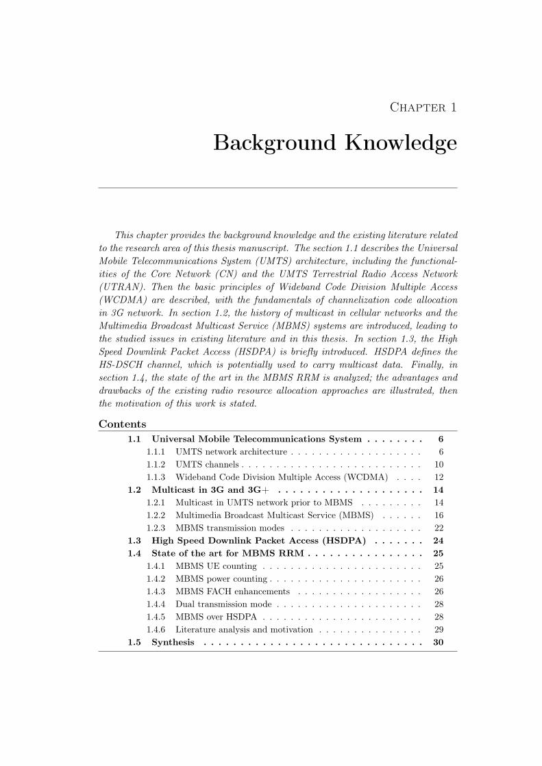
This chapter provides the background knowledge and the existing literature relatedto the research area of this thesis manuscript. The section 1.1 describes the UniversalMobile Telecommunications System (UMTS) architecture, including the functional-ities of the Core Network (CN) and the UMTS Terrestrial Radio Access Network(UTRAN). Then the basic principles of Wideband Code Division Multiple Access(WCDMA) are described, with the fundamentals of channelization code allocationin 3G network. In section 1.2, the history of multicast in cellular networks and theMultimedia Broadcast Multicast Service (MBMS) systems are introduced, leading tothe studied issues in existing literature and in this thesis. In section 1.3, the HighSpeed Downlink Packet Access (HSDPA) is briefly introduced. HSDPA defines theHS-DSCH channel, which is potentially used to carry multicast data. Finally, insection 1.4, the state of the art in the MBMS RRM is analyzed; the advantages anddrawbacks of the existing radio resource allocation approaches are illustrated, thenthe motivation of this work is stated.
Contents1.1 Universal Mobile Telecommunications System . . . . . . . . 6
1.1.1 UMTS network architecture . . . . . . . . . . . . . . . . . . . 61.1.2 UMTS channels . . . . . . . . . . . . . . . . . . . . . . . . . . 101.1.3 Wideband Code Division Multiple Access (WCDMA) . . . . 12
1.2 Multicast in 3G and 3G+ . . . . . . . . . . . . . . . . . . . . 141.2.1 Multicast in UMTS network prior to MBMS . . . . . . . . . 141.2.2 Multimedia Broadcast Multicast Service (MBMS) . . . . . . 161.2.3 MBMS transmission modes . . . . . . . . . . . . . . . . . . . 22
1.3 High Speed Downlink Packet Access (HSDPA) . . . . . . . 241.4 State of the art for MBMS RRM . . . . . . . . . . . . . . . . 25
1.4.1 MBMS UE counting . . . . . . . . . . . . . . . . . . . . . . . 251.4.2 MBMS power counting . . . . . . . . . . . . . . . . . . . . . . 261.4.3 MBMS FACH enhancements . . . . . . . . . . . . . . . . . . 261.4.4 Dual transmission mode . . . . . . . . . . . . . . . . . . . . . 281.4.5 MBMS over HSDPA . . . . . . . . . . . . . . . . . . . . . . . 281.4.6 Literature analysis and motivation . . . . . . . . . . . . . . . 29
1.5 Synthesis . . . . . . . . . . . . . . . . . . . . . . . . . . . . . . 30

6 Chapter 1. Background Knowledge
1.1 Universal Mobile Telecommunications System
The throughput limitations of the Global System for Mobile communications(GSM) led the International Telecommunications Union (ITU) to initiate work on anew worldwide standard, called 3G for the third generation network. The 3G Part-nership Project (3GPP) develops the Universal Mobile Telecommunications System(UMTS) [53] that delivers high-bandwidth data and voice services to mobile usersand mobile web data. UMTS is based on Wideband-Code Division Multiple Ac-cess (W-CDMA) for the radio part and inherits of the GSM/General Packet RadioService (GPRS) topology for the network backbone.
1.1.1 UMTS network architecture
Figure 1.1 shows the architecture of a UMTS network. It consists of three parts:the Core Network (CN), the UMTS Terrestrial Radio Access Network (UTRAN)and the User Equipment (UE). The CN is responsible for switching/routing voice,inter-system handover, gateway to other networks (fixed or wireless), and performlocation management when there is no dedicated links between the UE and theUTRAN. The UTRAN handles all radio-related functionalities, and operates inFrequency Division Duplex (FDD) or Time Division Duplex (TDD) modes usingWCDMA protocol. The UE is the equipment used by the user to access the UMTSservices.
Node B
Node B
Node B
Node B
Iub
SGSN
MSC/VLR GMSC
GGSN
External
Networks
Internet
UTRAN
Core Network
Gn/Gp
BM-SC
Gi:data Gmb
HLR/AUC
Gmb: control plan functions
Gi: bearer plan
Gp: only applied when SGSN and
GGSN are in different PLMNs
Content Provider
Multicast/Broadcast Source
RNC
RNC
UE
PS Domain
CS Domain
Uu
Content
Provider
Multicast
Broadcast
Source
Iu
UE
UE
Figure 1.1: UMTS network architecture

1.1. Universal Mobile Telecommunications System 7
1.1.1.1 Core Network
The CN is logically divided into two service domains: the Circuit-Switched (CS)service domain and the Packet-Switched (PS) service domain. The CS domain han-dles the voice-related traffic, while the PS domain handles the packet transfer. In theCS domain, the network includes the Mobile Switching Center (MSC), the VisitorLocation Register (VLR) and the Gateway Mobile Switching Center (GMSC). ThePS domain consists of the Gateway GPRS Support Node (GGSN) and the ServingGPRS Support Node (SGSN). Other network elements, such as the Home LocationRegister (HLR) and the Authentication Center (AUC) are shared by both domains.
1.1.1.2 UTRAN
The UTRAN provides the air interface for UE. As shown in Figure 1.1, theUTRAN consists of several Radio Network Subsystems (RNS). Each RNS is con-trolled by a Radio Network Controller (RNC) and has several Node B. Each NodeB can control several antennas and each antenna covers an area called a radio cell.The UE can directly communicate with one or more antennas (when the UE is inhandover procedure). The radio resources control is implemented through a dis-tributed architecture; each RNC is connected with the CN over the interface namedIu and with a Node B over the interface named Iub.
Radio Network Controller The RNC is a key element within the UTRAN asit controls all the radio resources. A RNC is responsible for a wide range of tasks[72].
– Admission control: in the CDMA system, it is very important to keep theinterference below a certain level. The RNC calculates the traffic within eachcell, and then it decides to accept or reject the new coming calls.
– Power control: the RNC only performs the outer loop power control. Thismeans that the RNC controls the transmission power in one cell on the basisof the interference received from the other neighbor cells. While the fast powercontrol is performed by a Node B 1500 times per second, the outer loop powercontrol helps the RNC to minimize the interference between the neighbor cells.
– Radio bearer setup and release: the RNC has to set up, maintain andrelease a logical data connection to a UE. This connection is called UMTSradio bearer.
– Radio resource control: the RNC controls all radio resources of the cellsconnected to it via a Node B. This task includes the interference control andload measurements.
– Handover control: based on the downlink/uplink signal strength and thesignal-to-interference ratio received by the UE and the Node B, the RNC can
8 Chapter 1. Background Knowledge
decide if the current cell is suitable for a given connection. When the RNCdecides to handover, it informs the new cell and the UE.
To achieve above tasks, one physical RNC contains three logical functionalities[54]:
– CRNC: the Controlling RNC (CRNC) controls the resources of one Node B.It performs the load and congestion control within the cells of the Node B.Besides, a CRNC executes the admission control and the code allocation toestablish new radio links in these cells.
– SRNC: the Serving RNC serves a particular UE and manages the connections(to/from the CN) with that UE.
– DRNC: the Drift RNC fulfills a similar role to the SRNC except that it isinvolved only in the case of soft handover.
The difference between the CRNC, SRNC and DRNC is that the CRNC islogically tied to the Node B, not to the connections. On the contrary, the SRNCand the DRNC are tied to the connections with the UE, which implies that theCRNC manages the common and the shared resource while the SRNC and theDRNC manage the dedicated resources.
Node B The Node B is the base station and provides the radio coverage to oneor more cells. It is connected directly with the UE via the WCDMA air accessingtechnology. An important task of the Node B is the inner loop power control. TheNode B measures the link quality and the signal strength, it manages the air interfacetransmission and reception, the modulation and the demodulation, the physicalchannel coding, etc. With the emergence of High Speed Downlink Packet Access(HSDPA), the Node B even handles some logic functionalities (e.g. retransmission)for lower response times.
1.1.1.3 NAS Stratum and AS Stratum
Vertically, there are two strata in the UMTS signaling protocol stack: the Non-Access Stratum (NAS) and the Access Stratum (AS). The NAS protocols are appliedbetween the UE and the core network, for which the access stratum acts as a re-lay. The UMTS non-access stratum consists in the Connection Management (CM),the Session Management (SM), the Mobility Management (MM), and the GPRSMobility Management (GMM).
The access stratum consists of three layers. The layer 1 is the Physical Layer(PHY), the layer 2 consists of the Radio Link Control (RLC) and the Medium AccessControl (MAC). The layer 3 is the Radio Resource Control (RRC).
The layer 1 service is the physical layer. It is responsible for transporting the
1.1. Universal Mobile Telecommunications System 9
data received from the higher layers over the physical channels. It hides all detailsof the underlying physical media, and provides the transport channels to the MAClayer. The PHY layer provides transport channels to the L2/MAC layer. Theconcept of channels will be introduced later.
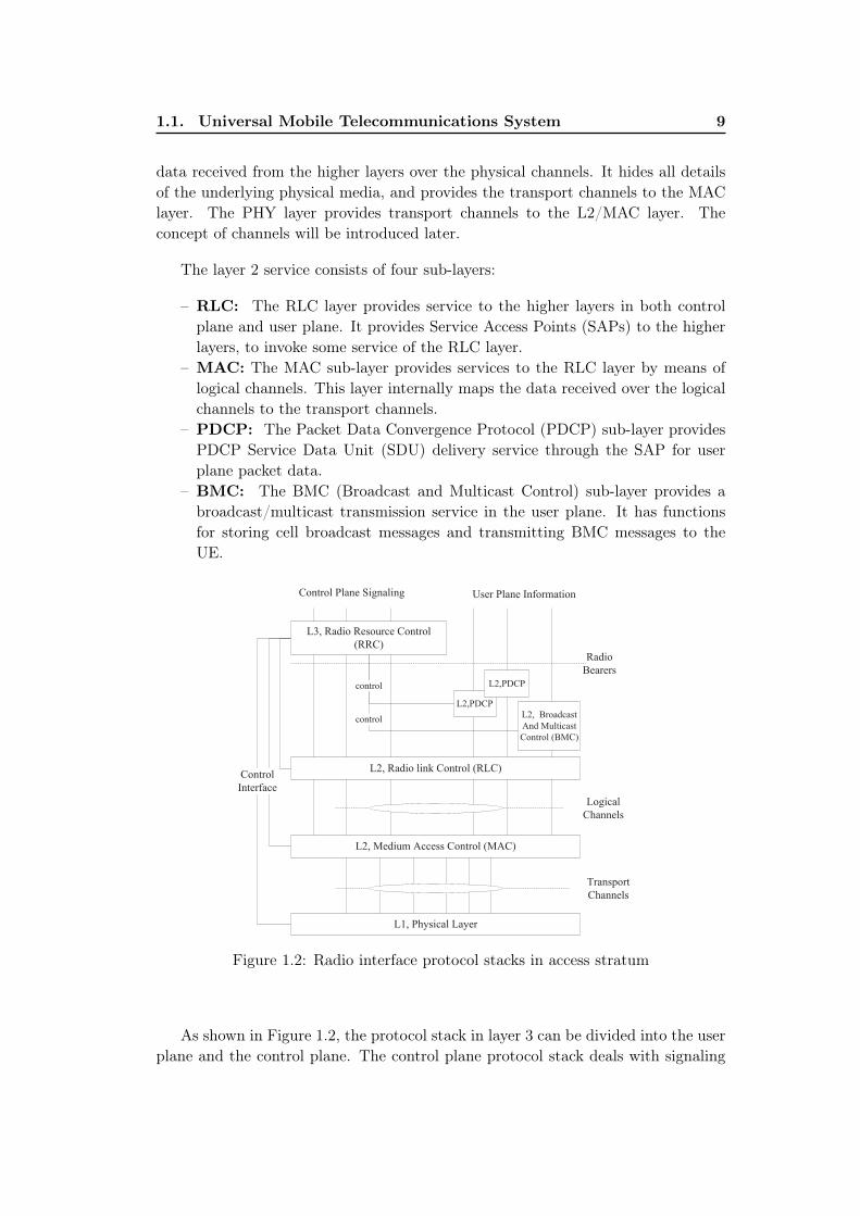
The layer 2 service consists of four sub-layers:
– RLC: The RLC layer provides service to the higher layers in both controlplane and user plane. It provides Service Access Points (SAPs) to the higherlayers, to invoke some service of the RLC layer.
– MAC: The MAC sub-layer provides services to the RLC layer by means oflogical channels. This layer internally maps the data received over the logicalchannels to the transport channels.
– PDCP: The Packet Data Convergence Protocol (PDCP) sub-layer providesPDCP Service Data Unit (SDU) delivery service through the SAP for userplane packet data.
– BMC: The BMC (Broadcast and Multicast Control) sub-layer provides abroadcast/multicast transmission service in the user plane. It has functionsfor storing cell broadcast messages and transmitting BMC messages to theUE.
L1, Physical Layer
L2, Medium Access Control (MAC)
L2, Radio link Control (RLC)
L3, Radio Resource Control
(RRC)
Control
Interface
Transport
Channels
Logical
Channels
Control Plane Signaling User Plane Information
L2, Broadcast
And Multicast
Control (BMC)
L2,PDCP
L2,PDCP
control
control
Radio
Bearers
Figure 1.2: Radio interface protocol stacks in access stratum
As shown in Figure 1.2, the protocol stack in layer 3 can be divided into the userplane and the control plane. The control plane protocol stack deals with signaling

10 Chapter 1. Background Knowledge
protocol. For example, the Radio Resource Control (RRC) protocol is part of thecontrol plane, which carries the network signaling messages. The user plane protocolstack deals with user protocols, it carries the data streams from/to the user.
1.1.2 UMTS channels
The UMTS channels can be classified in terms of functionalities, data flow di-rection and sharing. In terms of data flow direction, the downlink channels aretransmitted by the UTRAN and received by the UE, while the uplink channels aretransmitted by the UE and received by the UTRAN. In terms of sharing mechanismamong UE, the common channels send information toward and from multiple UE,while the dedicated channels send information to and from a single UE. In termsof functions, there are the logical channels, the transport channels and the physicalchannels (see Figure 1.2).
Logical channels The logical channels provide the data transfer service of theMAC layer. The logical channel type is defined by its content and the kind of offereddata service. A general classification of logical channel is into two groups: the controlchannels and the traffic channels. The control channels are used to transfer controlplane information, and the traffic channels for the user plan information.
Transport channels The MAC layer provides the logical channel to transportchannel conversion. The connections between the logical channels and the transportchannels are shown in Figure 1.3.
Figure 1.3: Logical channel to transport channel mapping
Different transport channels are defined from the type of information transferredby that channel. The transport channels can be subdivided into the common trans-port channels, the dedicated transport channels and the shared transport channels.The common transport channel is a resource divided between all or a group of usersin a cell, whereas a dedicated transport channel resource, identified by a certaincode on a certain frequency, is reserved for a single user only. The common channelsare the Random Access Channel (RACH) in the uplink and the Forward AccessChannel (FACH) in the downlink. The common channels do not have a feedback
1.1. Universal Mobile Telecommunications System 11
channel, and cannot use the fast closed loop power control, but only the open looppower control or fixed power. Therefore the link level performance of the commonchannels is not as good as the dedicated channels, and the common channels gener-ate more interference than the dedicated channels. The Dedicated Channel (DCH)is a bi-direction channel with both uplink and downlink connections. Because ofthe feedback channel, the fast power control and the soft handover can be used.These features improve their radio performance and consequently less interferenceis generated than with common channels.
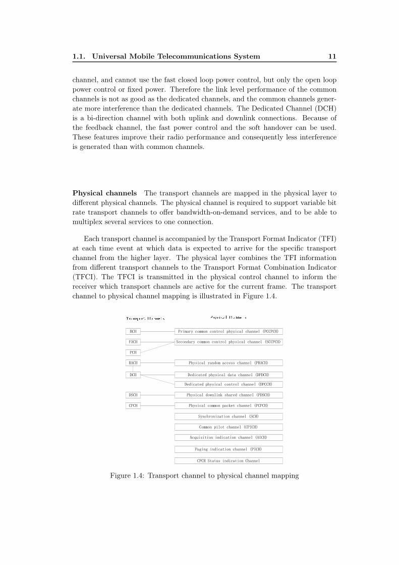
Physical channels The transport channels are mapped in the physical layer todifferent physical channels. The physical channel is required to support variable bitrate transport channels to offer bandwidth-on-demand services, and to be able tomultiplex several services to one connection.
Each transport channel is accompanied by the Transport Format Indicator (TFI)at each time event at which data is expected to arrive for the specific transportchannel from the higher layer. The physical layer combines the TFI informationfrom different transport channels to the Transport Format Combination Indicator(TFCI). The TFCI is transmitted in the physical control channel to inform thereceiver which transport channels are active for the current frame. The transportchannel to physical channel mapping is illustrated in Figure 1.4.
BCH Primary common control physical channel (PCCPCH)
FACH Secondary common control physical channel (SCCPCH)
PCH
RACH Physical random access channel (PRACH)
DCH Dedicated physical data channel (DPDCH)
Dedicated physical control channel (DPCCH)
DSCH Physical downlink shared channel (PDSCH)
CPCH Physical common packet channel (PCPCH)
Synchronization channel (SCH)
Common pilot channel (CPICH)
Acquisition indication channel (AICH)
Paging indication channel (PICH)
CPCH Status indication Channel
Figure 1.4: Transport channel to physical channel mapping
12 Chapter 1. Background Knowledge
1.1.3 Wideband Code Division Multiple Access (WCDMA)
In the radio accessing technologies, one of the basic concepts is to allow severaltransmitters to send information simultaneously over the radio link. It means toshare a band of frequencies, i.e. bandwidth between several users. The three mostimportant families of radio access schemes are: Frequency Division Multiple Access(FDMA), Time Division Multiple Access (TDMA) and Code Division Multiple Ac-cess (CDMA). These three mechanisms subdivide radio resources in the frequency,time and code domains, respectively.
WCDMA is a Wideband Direct-Sequence Code Division Multiple Access (DS-CDMA) system, i.e. user information bits are spread over a wide bandwidth bymultiplying the user data with quasi-random bits (called chips) derived from CDMAspreading codes. In WCDMA, all users use the same frequency band; to separatedifferent users, the codes used for spreading should be (quasi) orthogonal, i.e. theircross-correlation should be (almost) zero. The chip rate of 3.84 Mchip/s leads to acarrier bandwidth of approximately 5 Mhz. DS-CDMA systems with a bandwidthof about 1 MHz are commonly referred to as narrowband CDMA systems. Theinherently wide carrier bandwidth of WCDMA supports high user data rates andalso has certain performance benefits, such as increased multipath diversity.
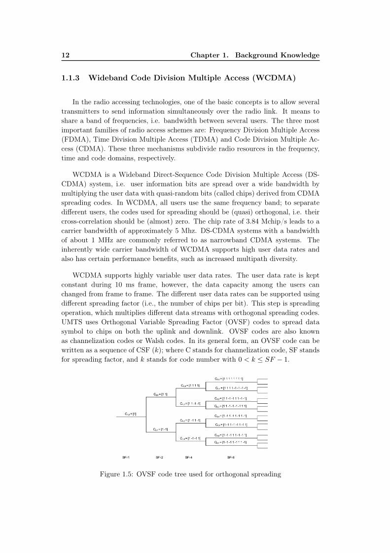
WCDMA supports highly variable user data rates. The user data rate is keptconstant during 10 ms frame, however, the data capacity among the users canchanged from frame to frame. The different user data rates can be supported usingdifferent spreading factor (i.e., the number of chips per bit). This step is spreadingoperation, which multiplies different data streams with orthogonal spreading codes.UMTS uses Orthogonal Variable Spreading Factor (OVSF) codes to spread datasymbol to chips on both the uplink and downlink. OVSF codes are also knownas channelization codes or Walsh codes. In its general form, an OVSF code can bewritten as a sequence of CSF (k); where C stands for channelization code, SF standsfor spreading factor, and k stands for code number with 0 < k ≤ SF − 1.
Figure 1.5: OVSF code tree used for orthogonal spreading

1.1. Universal Mobile Telecommunications System 13
The OVSF codes are generated from a code tree as shown in Figure 1.5. It beginswith the first generation one-bit code C1(0) = 1; where the subscript 1 stands forspreading factor 1, and (0) stands for code number 0. The second generation consistsof two codes: C2(0) and C2(1). They are two-bit codes with a spreading factor of 2.The third and fourth generations consist of four-bit and eight-bit codes numberingof four and eight respectively. The code tree can go up to 10 generations with the10th generation having 512 codes. For a given code tree generation, the spreadingfactor is equal to the number of codes. The following functions illustrate how theOVSF codes are generated:
C1(0) = 1 (1.1)[C2(0)
C2(1)
]=
[C1(0) C1(0)
C1(0) −C1(0)
]=
[1 1
1 −1
](1.2)
C4(0)
C4(1)
C4(2)
C4(3)
=
C2(0) C2(0)
C2(0) −C2(0)
C2(1) C2(1)
C2(1) −C2(1)
=
1 1 1 1
1 1 −1 −11 −1 1 −11 −1 −1 1
(1.3)
Two sequences are said to be orthogonal to each other if they have zero cross-correlation. In the OVSF code tree, two codes are orthogonal if and only if neithercode lies on the same path from the other code to the tree root. Graphically, twocodes are non orthogonal if they belong to the same branch of the tree. For example,if the code C4(0) is assigned to a user, the codes C1(0), C2(0), C8(0), C8(1) and soon, cannot be assigned to any other user in the same cell. In this way, OVSF codesfor different channels in the same cell are carefully chosen in order to be mutuallyorthogonal to each other, this restricts the number of available codes for a givencell.
With a given OVSF code, WCDMA performs the orthogonal spreading by mul-tiplying each encoded symbol with a code, meaning that one symbol is representedby multiple chips. e.g. a Spreading Factor (SF) of 4 means 4 chips per symbol,while a SF of 256 means 256 chips per symbol. The chip rate is kept in constant at3.84 Mcps(chips per second), and the ratio of chip rate and symbol rate is knownas the spreading factor.
SF =ChipRate
Symbol Rate=
3.84Mcps
Symbol Rate(1.4)
Therefore, high-rate transmissions use low spreading factor while low-rate trans-missions use high spreading factors. For example, for voice with a symbol rate of60 ksps, the 64-bit OVSF code used for spreading runs 64 times faster than thesymbol, making the spread symbol run at 3.84 Mcps. For data with a symbol rate
14 Chapter 1. Background Knowledge
of 960 ksps, the 4-bit OVSF code used for spreading runs four times faster thanthe symbol, resulting in again a spread symbol chip rate of 3.84 Mcps. Spreadingfactors can be range from 4 to 512 for the downlink and 4 to 256 for the uplink.
1.2 Multicast in 3G and 3G+
Traditionally, data communications concerns two entities: a transmitter and areceiver. Nowadays, with the introduction of mobile streaming, video conferencingetc, there is an increasing demand of traffic between one transmitter and manyreceivers, or even many transmitters and many receivers. Hence, efficient broadcastand multicast communications are required.
In broadcast, a message is sent to every possible destination. It is unknown thatif only a few receivers are interested in the message. In a wireless mobile network,broadcast transmission not only wastes the network resources but also the receiverresources, since the receiver, whom are not interested in the broadcast data, mustconsume energy in order to process useless data.
Multicast is more efficient in terms of network and receiver resources than broad-cast. Multicast data delivery increases the network efficiency and decreases theserver load by sending one data stream to several particular destinations. Whenthe network is aware of the fact that multiple receivers are targeted, it creates adistribution tree from the transmitter towards all receivers overlaying the networktopology. The network will duplicate the data only at branching points of the treetowards the receivers. Thus, instead of sending many streams from the transmitter,one to each receiver, multicast lets all receivers listen to the same stream and avoidsprocessing overheads replication at the source on the same link. Multicast requiresadditional mechanisms for group maintenance while broadcast does not.
1.2.1 Multicast in UMTS network prior to MBMS
Two services for transmitting data from a single source to several destinationswere defined prior to MBMS: the Cell Broadcast Service (CBS) and the IP multicastservice.
Since Release 4, the CBS service (CBS: Cell Broadcast Service) [14, 10] allows lowbit-rate unacknowledged messages to be transmitted to all receivers in a particulararea. The CBS broadcasts each message periodically, at a frequency and durationarranged with the information provider. The CBS, however, is targeted to textmessaging and without any QoS, therefore, it is unsuitable for high bandwidthmultimedia services.

1.2. Multicast in 3G and 3G+ 15
The IP Multicast service [3, 4] is defined since Release 99. It allows IP appli-cations to send data to a set of recipients (a multicast group) specified by an IPaddress. Any UE may join or leave a multicast group without restrictions. Release99 IP multicast is implemented by separately sending each packet from the GGSNto each UE, therefore, no sharing gains are achieved, and high bandwidth multime-dia services remain expensive. The IP multicast traffic can be received by mobilesubscribers already. However, the IP multicast does not allow to share radio or corenetwork resource hence no optimized transport solution exists.
In the initial UMTS multicast design [51], 3GPP decided to terminate the IPmulticast routing protocol in the GGSN. With this design, GGSN serves as a ren-dezvous point routers. Also, GGSN serves as a router Internet Group ManagementProtocol (IGMP) designated and performs IGMP signaling on point-to-point packet-data channels. IGMP signaling is performed in the network user plane, that meansit is seen as data traffic for the UMTS network. Multicast data is forwarded tothe UMTS terminal on point-to-point packet-data channels, i.e. unicast distribu-tion. The GGSN manufacturer can choose which IP multicast routing protocol tosupport. Only the UE and the GGSN are multicast compatible in this design. Asshown in Figure 1.6, the distribution tree by the IP multicast service allows thenetwork to treat multicast traffic in the same manner as unicast traffic.
Figure 1.6: Multicast duplication in UMTS network prior to MBMS [51]
To send and receive multicast data, the terminal firstly needs to perform a GPRS

16 Chapter 1. Background Knowledge
attach, then the terminal must establish a packet data channel with the GGSN. TheUMTS terminal is now part of the IGMP environment, and can join and leave themulticast groups using normal IGMP signaling. Finally the terminal must establishone or more packet data channels (Packet Data Protocol (PDP) context activation)for the multicast data flows.
As shown in Figure 1.6, this multicast architecture reduces the load on a wirelesssource. The source only needs to send one copy of the multicast data to the GGSN.Then the GGSN replicates and forwards the packet on to the multicast distributiontree. However, the UMTS multicast source does not receive any information frommulticast members. Thus even if the multicast group does not have any members,the source will continue transmitting its multicast data to the GGSN. The source isnot aware of the empty state of the multicast group. A modified signaling connectionbetween the GGSN and the source can avoid this situation. This architecture alsoimposes a high strain on the GGSN. The GGSN already has the responsibility formany complex mechanisms, thus it is important to avoid turning the GGSN intothe UMTS networks bottleneck.
The drawback of this multicast architecture is that it requires more networkresources than unicast distribution of the same data. Moreover, due to the factthat GGSN serves as a designated router, detailed membership information must bestored in the GGSN for the UMTS Terminals. This might work efficiently when thenumber of the users requesting to join the multicast group is low. But when a greatnumber of users request the same MBMS service, the network may then collapsewith huge capacity and processing requirements in the core and the radio network.
With these shortcomings in mind, 3GPP defined MBMS to decrease the amountof data within the network. It aims at offering an efficient way to transmit datafrom a single source to multiple destinations over the radio network. MBMS istransparent to end users (they have the same experience as with Point-to-Pointconnections) while saving resources on the UE side.
1.2.2 Multimedia Broadcast Multicast Service (MBMS)
To support efficient distribution of multicast multimedia services over mobile net-working, the 3GPP specified the Multimedia Broadcast/Multicast Service (MBMS)since Release 6 specifications [18, 16, 17]. The main advantage of MBMS is thatit allows many receivers in the same radio cell to be served by a common signaltransmission facility, or bearer, thus saving radio resources.

1.2. Multicast in 3G and 3G+ 17
1.2.2.1 MBMS system architecture
MBMS integrates broadcast/multicast transmission capabilities into 3G serviceand network infrastructures. In UMTS network, bandwidth is a limited resource.MBMS supports the network to transmit the data only once over a particular route.All users that belong to the same multicast group can receive service simultane-ously on the same frequency and time slot. As shown in Figure 1.7, the existingPacket-Switched (PS) domain functional entities (UE, GGSN, SGSN, UTRAN andGERAN) and MBMS-specific interface functions (Gmb) are enhanced to supportthe MBMS bearer service.
Content Provider Multicast/Broadcast Source
UE SGSN
UE GERAN
UTRAN
HLR
GGSN BM-SC -
Content Provider Multicast Broadcast Source
Uu Iu
Iu / Gb Um
Gr
Gn / Gp
Gi
Gmb
Other PLMN
BM-SC
Mz
Figure 1.7: Enhancement of MBMS in UMTS [18]
Besides, MBMS system is realized by one additional component named Broad-cast Multicast Service Center (BM-SC). The BM-SC is a MBMS specific functionalentity supporting various MBMS user service such as schedule and deliver. It per-forms following functions:
– Membership function.– Session and Transmission (in radio access network) function.– Proxy and Transport (in CN) function.– Service Announcement function.– Security function.
With these enhancement, the MBMS feature is split into the MBMS BearerService and the MBMS User Service.
The MBMS Bearer Service includes a Multicast and a Broadcast Mode. TheMBMS Bearer Service uses IP multicast addresses for the IP flows. The advan-tage of the MBMS Bearer Service compared to unicast bearer services (interactive,streaming, etc.) is, that the transmission resources in the core and radio networkare shared. One MBMS packet flow is replicated by GGSN, SGSN and RNC (see

18 Chapter 1. Background Knowledge
Figure 1.7). MBMS may use an advanced counting scheme to decide the most effi-cient system usage between using (zero, one or more) dedicated (i.e. unicast) radiochannels and using one common (i.e. broadcast) radio channel.
The MBMS User Service is basically the MBMS Service Layer and offers aStreaming and a Download Delivery Method. The Streaming Delivery methodcan be used for continuous transmissions like Mobile TV services. The DownloadMethod is intended for Download and Play services. To increase the transmissionreliability, an application layer FEC code may be used. Furthermore, a file-repairservice may be offered to complement the download delivery method.
1.2.2.2 MBMS services
According to the different quality of service (QoS) types, the services targetedby MBMS are classified into three categories.
– Streaming service: Continuous media such as audio and video, plus supple-mentary text and images, similar to TV channels but enhanced with multime-dia content. Images may also be used for banner images that advertise someproduct or service. These static media need to be synchronized and displayedwith audio/video streams.
– File Download services: Reliable binary data transfers without strict delayconstraints over an MBMS bearer, similar to conventional file transfers butwith multiple receivers. It is necessary that the user receives all the data sentin order to experience the service.
– Carousel service: Combination of streaming service and file download ser-vice, similar to stock quote ticker tapes. The target media of this service isonly static media (e.g. text and/or still images). Time synchronization withother media is also required, e.g. text objects are delivered and updated fromtime to time. Images are also collated to display low frame-rate video. Thebenefit of this service is that it is possible over a low bit-rate bearer. An ex-ample of the carousel service is a ’ticker-tape’ type service in which the datais provided to the user repetitively and updated at certain times to reflectchanging circumstances.
Therefore, potential MBMS applications include not only cellular band broadcastmobile television; but also cellular band broadcast mobile radio and area-specifictarget mobile advertising, etc. These potential applications in MBMS are shown inTable 1.1.

1.2. Multicast in 3G and 3G+ 19
Service type Service Content Potential Application
News clip Text distribution News/sport highlights, movietrailers, economics, etc
Localized service Text, video Tourist information, restaurant,etc
Audio stream Audio, timed text Music, live traffic information,voice notification
Content distribution Downloading, video,audio
Software updates, etc
Video clip Video and audiostreams, timed text
Live events, interactive televisionvoting
Table 1.1: MBMS services and potential applications
1.2.2.3 MBMS service distribution procedures
MBMS supports broadcast and multicast services in mobile environment. Itdefines the transmission of service through Point-to-Multipoint method. With thismanner, the same data is transmitted from a single source entity to multiple recip-ients while sharing the core and radio network resources.
The broadcast service is a unidirectional point-to-multipoint transmission ser-vice, from a single source entity to all users in a broadcast service area. It does notneed subscription. The broadcast service is free of charge and does not need spe-cific activation requirements. Broadcast supports streaming service while the CellBroadcast Service (CBS) is intended for messages only.
The multicast service allows the unidirectional Point-to-Multipoint transmissionof multimedia data from a single source point to a multicast group in a particularservice area. Unlike the broadcast service, the multicast service requires a subscrip-tion to the multicast group. Users need to be notified of the service availability byservice announcements. Then they need to join the corresponding multicast groupby sending joining messages. From the network point of view, the same content canbe provided in a Point-to-Point fashion if there are not enough users to justify thehigh power transmission of the Point-to-Multipoint channel. Unlike the broadcast,users are expected to be charged for multicast service.
As shown in Figure 1.8, there are several procedures to enable MBMS multicastservice. The subscription, joining and leaving phase are performed individually foreach single user. The other procedures are performed for all users interested in amulticast service. The sequence of procedures may repeat if it is necessary.

20 Chapter 1. Background Knowledge
Subscri ption
Joining
Service announcement
Data transfer
Leaving
MBMS notification
Session start
Session Stop
Figure 1.8: Multicast procedure [16]
– Subscription: The subscription is the agreement of a user to receive ser-vice(s) offered by the operator, which allows the user to receive the relatedMBMS multicast service in further transmission. The subscription informationis recorded in the BM-SC. This information allows to establish the relationshipbetween users and the service provider.
– Service announcement: By receiving MBMS service announcement, usersshall discover the range of MBMS services and service availability. This mech-anism distributes to users information about the service content, parametersrequired for service activation (e.g. IP multicast address(es)) and possiblyother service related parameters (e.g. service start time).
– Joining: The joining is an activation message sent by the UE. In this pro-cedure, the UE indicates to the network that it wants to receive multicastmode data of a specific MBMS service. This activation procedure allows asubscriber to become a member of a multicast group, and to be recorded bythe network.
– Session Start: This step is the point at which the BM-SC is ready to senddata. A session start message is sent for each MBMS bearer service. Thiscan be identified with the start of a multicast session. Session start occursindependently of activation of the service by the user, which means, a givenuser may join the service before or after session start. Session start is thetrigger for radio/network resource establishment for MBMS data transfer.
– MBMS notification: It informs the UEs about forthcoming (and poten-tially about ongoing) MBMS multicast data transfer.
– Data transfer: In this procedure, MBMS data are transferred to UEs. Theuser data and control messages are transmitted, as well as the error recoverypackets if it is necessary (e.g. fading conditions or handover).

1.2. Multicast in 3G and 3G+ 21
– Session Stop: This step is the point at which there will be no more data tosend for a period of time. The bearer resources are released at session stop.
– Leaving: In this process a subscriber leaves, i.e. stops being a member. ThenMBMS multicast is deactivated by the user.
Figure 1.9 shows a timeline example of the multicast service procedures, in whichtwo users join and receive data flow from the same service sequentially. It is il-lustrated that the subscription, joining, leaving, service announcements as well asMBMS notification can run in parallel to other phases. Moreover, there are threeimportant periods related with the management of radio resource for MBMS service.
Figure 1.9: An example of two users receiving MBMS multicast service
22 Chapter 1. Background Knowledge
– Period between Service Announcement and Joining. The Joiningtime depends on the user’s choice and the possible user is in response to aservice announcement. Users will typically join at a chosen time so that theperiod between announcement and joining may be very long or very short. Inorder to avoid overload situations being caused by many users attempting tojoin in a short period of time, the UE shall be able to use parameters sent bythe BM-SC in the service announcement to randomize the joining time.
– Period between Joining and Session Start. Some MBMS multicastservices may be ’always on’. In this case, Joining can take place immediatelyafter Service Announcement and possibly many hours before, or after, thesession start. In other cases, if a Session Start time is known, Joining maytake place immediately before Session Start or after Session Start. For theseservices, the announcement may contain some indication of a time period atwhich users and UEs should use to choose a time to Join the MBMS bearerservice.
– Period between Session Start and First Data Arrival. Session Startindicates that the transmission is about to start, then the network actionswill take place for the arrival of first data. Therefore, the time delay betweena Session Start indication and actual data arrival should be long enough forthese network actions, e.g. provision of service information to the UTRAN,and establishment of the network and radio resources. Session Start may betriggered by an explicit notification from the BM-SC.
1.2.3 MBMS transmission modes
MBMS defines two transmission modes in UTRAN to provide MBMS multicastservice: point-to-point transmission (PTP) mode and point-to-multipoint trans-mission (PTM) mode. To carry the relevant MBMS data and signaling throughPTM mode, three new logical channels are added to Release 6. They are MBMSControl Channel (MCCH) carrying MBMS control signaling; MBMS Traffic Chan-nel (MTCH) carrying MBMS application data; and MBMS Scheduling Channel(MSCH) carrying MBMS scheduling information to support discontinuous recep-tion in the UE. MTCH is used to carry MBMS multicast data through PTM mode.
MTCH is a logical channel specifically used for a PTM downlink transmissionof user plane information between network and UEs. The user plane informationon MTCH is MBMS service specific and is sent to UEs in a cell with an activatedMBMS service [18]. MTCH maps to one transport channel named Forward AccessChannel (FACH) and then to physical channel named Secondary Common ControlPhysical Channel (SCCPCH) in the downlink direction. Initially, FACH is a down-link transport channel that carries control information to terminals known to belocated in the given cell. This is used, for example, after a random access messagehas been received by the base station through a Random Access Channel (RACH).

1.2. Multicast in 3G and 3G+ 23
!"#
$%"#
&'(
$)"'
*%"'
+""&"'
,)"'
,"'
,&,"'
,)"'
'+-,+"'
'+-&,+"'
,)"',)"'
,"',"'
Figure 1.10: MBMS transmission modes and channel mapping
Currently, MBMS defines the PTM transmission mode which supports to transmitdata packets on FACH. It aims at overcoming network congestion when a largernumber of users request the same service. For each service, only one FACH is re-quired for the transmission of service stream, while no traffic load on the uplinkconnections is required. FACH does not use fast power control (see section 1.1.1.2),and the transmitted messages should include band identification information to en-sure their correct reception. On one hand, the reliability of FACH transmissionis less than channels using a feedback channel for receiving quality. On the otherhand, PTM mode needs rather high-power level to reach all users in the cell sinceit lacks of physical layer feedback in uplink. One or several FACH(s) are carriedon the secondary common control physical channel (S-CCPCH); each FACH is sentwith a fixed data rate (depending on the traffic bandwidth).
The PTP mode uses the logical channel named Dedicated Traffic Channel (DTCH).DTCH is defined in the user plane and transfers the information of a given servicededicated to a single user. It exists both in the uplink and downlink direction.Different DTCH may coexist for a given UE whenever several services are providedsimultaneously (e.g. data and voice connections). Each DTCH serves one ded-icated UE, and maps to transport channel Dedicated Channel (DCH) then overthe downlink physical channel Downlink Physical Dedicated Channel (DPDCH).DCH is bi-directional with inner and outer loop power control. Because DCH is aPoint-to-Point channel, multiple DCHs are required for transferring common datato a multicast group. Since DCH can employ fast closed-loop power control, itcan achieve a highly reliable transmission quality. DCH also consists of an uplinkchannel, which is used to feedback power control information. RNC could controlthe state transitions between PTP and PTM modes which allows the radio networkto keep the efficient power utilization state. Hence it needs to transfer the trafficvolume between Cell_FACH and Cell_DCH and vice versa.
24 Chapter 1. Background Knowledge
1.3 High Speed Downlink Packet Access (HSDPA)
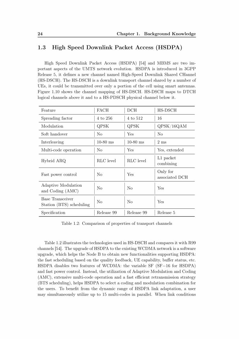
High Speed Downlink Packet Access (HSDPA) [54] and MBMS are two im-portant aspects of the UMTS network evolution. HSDPA is introduced in 3GPPRelease 5, it defines a new channel named High-Speed Downlink Shared CHannel(HS-DSCH). The HS-DSCH is a downlink transport channel shared by a number ofUEs, it could be transmitted over only a portion of the cell using smart antennas.Figure 1.10 shows the channel mapping of HS-DSCH. HS-DSCH maps to DTCHlogical channels above it and to a HS-PDSCH physical channel below it.
Feature FACH DCH HS-DSCH
Spreading factor 4 to 256 4 to 512 16
Modulation QPSK QPSK QPSK/16QAM
Soft handover No Yes No
Interleaving 10-80 ms 10-80 ms 2 ms
Multi-code operation No Yes Yes, extended
Hybrid ARQ RLC level RLC levelL1 packetcombining
Fast power control No YesOnly forassociated DCH
Adaptive ModulationNo No Yes
and Coding (AMC)
Base TransceiverNo No Yes
Station (BTS) scheduling
Specification Release 99 Release 99 Release 5
Table 1.2: Comparison of properties of transport channels
Table 1.2 illustrates the technologies used in HS-DSCH and compares it with R99channels [54]. The upgrade of HSDPA to the existing WCDMA network is a softwareupgrade, which helps the Node B to obtain new functionalities supporting HSDPA:the fast scheduling based on the quality feedback, UE capability, buffer status, etc.HSDPA disables two features of WCDMA: the variable SF (SF=16 for HSDPA)and fast power control. Instead, the utilization of Adaptive Modulation and Coding(AMC), extensive multi-code operation and a fast efficient retransmission strategy(BTS scheduling), helps HSDPA to select a coding and modulation combination forthe users. To benefit from the dynamic range of HSDPA link adaptation, a usermay simultaneously utilize up to 15 multi-codes in parallel. When link conditions
1.4. State of the art for MBMS RRM 25
are very favorable, based on the scheduling decisions done in the Node B, most ofthe cell capacity may be allocated to one user for a very short time. In this way,additional user throughout could be achieved, in general for free. The peak rateof HS-DSCH is up to 10 Mbps with 16 quadrature amplitude modulation (QAM).Therefore, HS-DSCH provides a more flexible and efficient method for utilizing radioresource management to achieve significant improvements on the downlink capacity,reduced network latency and higher data rates for packet data services.
Although Release 99 transport channels involving FACH and DCH, have alreadybeen standardized for MBMS multicast transmission, MBMS over HS-DSCH is stillan interesting research topic [73, 80, 25, 68, 31].
1.4 State of the art for MBMS RRM
This section introduces the related work in the study of radio resource allocationfor MBMS. In UTRAN, the sharing of limited radio resources among numeroususers per cell is constrained with more services subscriptions and higher requestedtraffic bandwidth. The RNC is responsible for the efficiency of transmission schemeselection. Before MBMS data transfer (see Figure 1.8), in the period between Joiningand Session Start, the RNC needs to choose the appropriate transmission schemesand relevant radio resource allocation. In the period between Session Start andFirst Data Arrival, the radio bearers are established for data transmission, aimingto achieve an efficient overall utilization of radio and network resources. Then duringthe MBMS session, the RNC should adapt to continuous changes in the dynamicwireless environments, optimally allocate radio resources and satisfy the servicerequirement in real-time, during which, the switch of MBMS transmission modes iscrucial to the allocation efficiency.
In particular, the Node B transmission power is a limited resource and shouldbe shared among all MBMS multicast users in a cell. Hence the power control isessential in order to minimize the power consumption, thus to eliminate intercellinterference and reserve cell capacity. When the number of subscribers for multicastservices and traffic requirement increases, the main concern in the development ofradio resource management for MBMS session is to serve the purpose of power saving(with or without lower QoS). The existing MBMS RRM techniques are presentedin following paragraphs.
1.4.1 MBMS UE counting
The 3GPP designed the MBMS UE Counting mechanism in TS 25.346 [18]. TheUE counting supports to determine the switching threshold between PTP and PTM

26 Chapter 1. Background Knowledge
modes based on the number of MBMS subscribers. This function is performed bythe RNC before MBMS data transfer. First, the RNC sends counting messagesto users in a given cell, then identifies the numbers of users by received countingresponse messages. When the number of users that wish to receive a multicastsession for a particular service is below an operator-defined threshold, the RNC willestablish PTP connections through the DCH channel(s). During MBMS servicetransmission, the switch from PTP to PTM resources should occur, when the usernumbers exceeds the predefined threshold, and vice versa. The study in [37] claimedthat the threshold is 7 UEs per cell, with the assumption that the FACH transmissionpower is set to 4 W. While in [56] the threshold is 5 UEs.
However, since the PTP transmission power would be different for different geo-graphic distribution of users, to determine the appropriate radio bearer only basedon the number of users is simply to implement but not sufficient.
1.4.2 MBMS power counting
The inefficiency of the UE counting and the power limitation motivated the3GPP to define the MBMS Power Counting (MPC) mechanism in TR 25.922 [15].This function aims to minimize the Node B power requirements during the trans-mission. The study under these assumptions is presented in [55], where the authorsfirst consider that the PTM transmission power remains as the same level to coverthe whole cell. Then the switching point between PTP and PTM modes is based onthe power consumption of PTP mode. When the estimated power consumption ofPTP mode in a cell is less than that for PTM, the network establishes PTP connec-tions. The switch from PTP to PTM occurs when the power exceeds the threshold,and vice versa. Furthermore, the study in [24] proposes a power control scheme forthe MBMS transmission channel selection among PTM and PTP modes. Later thiswork is analyzed in micro and macrocell environments [22].
MPC has limited flexibility because it only considers delivering service for allusers with full service quality; it does not support PTP and PTM for one serviceconcurrently. Therefore, when MBMS transmission power in one cell is near satura-tion, MPC does not provide alternative allocation scheme to save resource for newservice or new users to access into the network. These alternative schemes involvereducing power consumption by decreasing service’s quality, or applying flexiblepower allocation for PTM mode.
1.4.3 MBMS FACH enhancements
FACH is the only PTM channel that carries MTCH traffic. In conventional PTMdownlink transmissions, FACH does not support the fast power control. Therefore,
1.4. State of the art for MBMS RRM 27
in order to be received by all UEs throughout the cell, each FACH should be estab-lished at a fixed power level high enough to ensure the requested QoS in the wholecell. The following studies aim to increase the FACH efficiency.
1.4.3.1 Physical layer enhancement
As FACH power is limited, FACH transmission efficiency strongly depends onthe maximizing diversity. In [67], the authors propose a longer Transmission TimeInterval (TTI), using 80 ms instead of 20 ms as the FACH TTI for MBMS transmis-sion, thus to provide time diversity against fast fading. While longer TTI introducesmore complexity and larger memory space requirement in user side, to obtain macrodiversity in which a user receives the same signal from multiple transmitters locatedin different cells, the combing transmissions (soft and selection combing) is proposedfrom multiple cells [67]. Besides, the Spatio-Temporal Transmit Diversity (STTD)processing techniques exploit diversity in both spatial and temporal domains. It as-sumes two transmitting antennas and a single data stream in order to improve thesignal quality and reduce the power requirement. These statements are confirmedthrough analytical investigations in [12].
1.4.3.2 Dynamic power setting
Dynamic Power Setting (DPS) for PTM mode was initially proposed in [78].Instead of fixing the FACH power to cover the whole cell, the RNC dynamicallyadjusts the FACH power to just achieve the worst users of multicast group. Thistechnology aims to save the power efficiently in PTM mode. To support DPS, theMBMS users need to turn on measurement report mechanism while they are on theCell_FACH state. Based on such dynamic and periodic measurement reports, theNode B adjusts the transmission power for FACH [28].
1.4.3.3 Scalable FACH transmission
The multicast service delivery quality can be improved by adapting the scalabil-ity ratio (bit rate and frame rate) of multimedia streams through different codingstructures. This technology is also named as rate splitting because the service canbe split into several streams. The transmission schemes of multicast service aredivided into single layer (SL) and multilayer (ML) transmission schemes [52]. Forthe ML scheme, the service is scalable encoded by several flows; each flow has lowerbitrate and QoS requirements comparing to a nonscalable stream.
The scalable technology, integrated with FACH transmission (named S-FACHin this work), is initially proposed in [79]. Then it is further studied in [31]. In

28 Chapter 1. Background Knowledge
the scalable FACH transmission technology, to provide basic service quality, themost important stream (basic flow) is sent to all the users in the cell; then theless important streams (advanced flows) are only sent to users who have better linkqualities. For these users (e.g. the users near the Node B), the reception of advancedflows can enhance the service quality on top of the basic flow. The authors in [23]studied the performance of scalable FACH transmission in cells with site-to-sitedistance of 1 km. The simulation shows that a single 64 kbps stream carried by oneFACH channel requires the power of 7.6 W to cover the whole cell (95%). Whilefor a double stream transmission, only 5.8 W is required for transmitting two datastreams of 32 kbps through two FACHs, in which the basic flow with 95 % coveragerequests the power of 4.0 W, and 1.8 W for the advanced flow covering 50 % of thecell. Thus, 1.8 W can be saved through the Scalable FACH transmission.
However, the scalable FACH transmission involves certain negative results. Someusers which are near the cell edge will not be fully satisfied, as they only receive thebasic service quality. Besides, the utilization of the scalable transmission for MBMSmulticast is less flexible as it only supports PTM mode and with fixed coverageunder static assumption [79, 31]. Therefore, the gain of S-FACH is rather limitedas the Node B could not able to weigh the transmission power consumption and theusers’ satisfaction.
1.4.4 Dual transmission mode
Dual Transmission Mode (DTM) allows the co-existing usage of PTP and PTMmode for one MBMS service [28]. It adapts the FACH coverage for users with betterlink quality, while the users near the cell edge are served by DCHs. DTM is activeboth before and during MBMS transmission. The FACH coverage is dynamicallyadapted by changing its transmission power (i.e. Dynamic Power Setting for FACH),meanwhile the DCH connections are released or established for the rest of users.DTM enriches the candidate transmission modes for MBMS. The advantage of DTMis obvious during handover for single user. However, DTM does not consider theintegration with scalable transmission, and the simulation in [9] concluded thatDTM is only beneficial for up to 5 users with PTP connections. Therefore, onlyapplying FACH and DCH co-existing for transmission modes is limited not only inpower efficiency, but also in terms of channelization codes usage [24].
1.4.5 MBMS over HSDPA
The HSDPA as a means to deliver MBMS streaming is investigated by many re-searchers. The studies mainly focus on the scheduling and multi-resolution aspects(modulation and coding) [73, 31]. It is proved that with suitable packet scheduleralgorithm and hierarchical QAM constellations, MBMS over HSDPA can achieve a

1.4. State of the art for MBMS RRM 29
good fairness and capacity. Besides, some literature have studied the power utiliza-tion of MBMS transmission through HS-DSCH [68, 80, 25]. There are two methodsto allocate HS-DSCH power for carrying MBMS multicast data. The first methodconsiders the HS-DSCH transmission with fixed amount of power (e.g. 7 W [23, 31]).Then when the estimated power of FACH or DCH transmission will be more than7 W, the multicast service transmission will be carried by HS-DSCH. Otherwise,when the estimated FACH or DCH transmission power are less than 7 W, the trans-mission mode switch will be triggered, to transfer the multicast data by FACH orDCH, depending on which channel consumes less power. In the second method,after the power for common control channel and signaling channel are allocated, theNode B will allocate the rest of available power to HS-DSCH . In this method, theHS-DSCH power will dynamically change based on the available transmission powerand the serving service and users. In the study of HS-DSCH for MBMS [25, 68], thesecond method is used to estimate the required HS-DSCH power, then to compareit with the power of FACH and DCH, and to select the proper transmission modeby using the mode which is less power consuming. But none of these literature hasconsidered the co-existing usage with the UMTS R99 channels.
1.4.6 Literature analysis and motivation
Although MBMS RRM in 3G network and HSDPA has been well studied, thereare three main drawbacks in the existing allocation approaches. Firstly, the MBMSin 3G network has not been systematically analyzed, neither the problem complexitynor the problem characteristics. The existing approaches try to improve the RRMefficiency, rather than following systematic guidances. Therefore, almost all algo-rithms can only be compared with the standardized allocation approaches, whilerare study compares their performance with competitive algorithms.
Secondly, all existing approaches only consider the allocation scheme for mono-objective, i.e. to minimize the consumption of transmission power. Therefore, onlya one dimensional evaluation criterion is proposed in existing studies. However, thechannelization code is also a crucial limitation in UTRAN, which impacts the cellcapacity and data rate. While considering both these two radio resources will bringsignificant problem complexity in algorithm design as well as implementation.
Last but not least, the transmission modes in the existing approaches offer lim-ited flexibility regarding the dynamic mobile environments and radio resources con-sumption. For example, when the transmission power is saturated, the transmissionmode should be determined between transmission service i) through basic qualitylink with full coverage and ii) through advanced quality link with smaller coverage.When the transmission power is sufficient, meanwhile, the channel codes is also animportant but limited radio resource. Therefore, in case of channel codes saturation,the transmission mode should be selected among i) less power consumption scheme

30 Chapter 1. Background Knowledge
and ii) less occupation of channel codes.
To overcome these limitations mentioned above, we propose a Flexible RadioResource Management Model (F2R2M) which combines the flexible transmissionmode selection and the multimedia scalability. The contribution of this work isthree-fold: Firstly, a general model of the MBMS RRM problem is provided, whichabstracts the input parameter, decision parameter and optimization objectives. Inthis model, the mathematical formulation based on classical combinatorial optimiza-tion problem is developed. Then the fitness landscape analysis is conducted, whichproves the problem difficulties and guides the optimization strategies.
Secondly, based on the proposed model and the problem properties, we proposean allocation procedure with two-dimensional objective along with a lexicographic-order evaluation criteria to evaluate the quality of resources allocation in terms ofservice satisfaction and resource consumption. Hence the allocation approach isable to minimize the power consumption, and to save the channel code occupation.Finding the optimal solution which efficiently allocates the radio resource for MBMSmulticast service, while guarantees the Quality of Service (QoS), maintains theservice coverage and offers the cell capacity as high as possible.
Thirdly, our allocation approach offers higher flexibility in terms of allocationefficiency. It can self adapt to the dynamic user scenario in the mobile environment:the user number, the user distributions and the service requests which are differentfrom time to time. The proposed allocation approach is implemented, and the otherapproaches are reproduced, then they are applied to the same scenarios in the sameplatform; in this way, we offer a general test-bed to compare these algorithms undercommon situation.
1.5 Synthesis
This chapter provides the background knowledge and the existing literaturestudy related to the research area in this thesis manuscript.
The first section presented the fundamentals of UMTS. UMTS uses WCDMAas the radio access technology, which subdivides the radio resource in code domainfor simultaneous transmissions over the radio link. The high level architecture ofUMTS includes UE, UTRAN and CN. UTRAN takes in charge the radio resourceestablishment, reconfiguration and release. In these procedures, the channelizationcodes and the transmission power of channels are limited resource in UTRAN.
The second section introduced the MBMS framework and its features since theRelease 6. MBMS provides an efficient distribution platform for the multicast multi-media services transmission over mobile networks. MBMS defines the logical channel

1.5. Synthesis 31
MTCH to support the PTM transmission mode for multicast service, which savesthe unnecessary radio resource in UTRAN. MBMS also supports the PTP modefor multicast, which is carried by DCH channel. Following by which the HS-DSCHtransport channel defined in HSDPA is introduced. Then HS-DSCH is comparedwith the traditional MBMS transmission modes. The HS-DSCH feature is analyzedas an open issue for MBMS multicast carrier.
Based on the background knowledge, the related literature work in the field ofMBMS RRM study has been introduced. The advantages and the disadvantagesof these approaches are analyzed. It is found that the existing studies have thefollowing shortcomings:
1. Lack of systematic modeling of the targeting problem.
2. Lack of systematic analysis of the solution space for the targeting problem,therefore they can not prove whether the achieved radio resource assignmentis optimal or not.
3. Lack of enough flexibility and therefore they can only be beneficial in somescenarios but they have limitations in other scenarios.
With these in mind, the motivation of this work is declared:
1. To propose a general mathematical model to allow in-depth analysis for theMBMS RRM problem. The model should also be able to provide enoughflexibility to enable efficient radio resource allocation schemes.
2. To systematically analyze the problem complexity and the structure of thesolution space, so that the algorithm performance can be better evaluated.
3. To propose novel and practical algorithms, which aim to find the optimal radioresource assignments for arbitrary user scenarios in dynamic mobile environ-ment, considering both the throughput requirement and the power consump-tion limitation.
The proposed flexible radio resource management model for MBMS multicast servicewill be detailed in chapter 2.

Chapter 2
F2R2M: A Flexible Model forRRM of MBMS
This chapter will describe the first contribution: a general modeling of MBMSRRM problem named the Flexible Radio Resource Management Model (F2R2M).Based on this model, the target is to perform dynamic radio resource allocation formulticast service by using optimization approach. In terms of allocation scheme, thismodel provides the abstraction for the mixed usage of three transport channels, aswell as the abstraction for the scalable encoded multimedia stream, hence it offers theflexibility and possibility for high efficient radio resource utilization, and it satisfiesthe search complexity. In this model, a two-dimensional cost function is proposedwhich reflects the optimization for both the power consumption and the quality ofservice. A lexicographic evaluation criterion is also proposed to allow us to meet thethroughput requirement while at the same time to minimize the transmission power.Finally we obtain solution with proper service quality, low power and channelizationcode consumption, hence minimizing the cell interference and maximizing the cellcapacity.
Contents2.1 Model framework . . . . . . . . . . . . . . . . . . . . . . . . . 35
2.1.1 Phase 1: Parameter collection phase . . . . . . . . . . . . . . 352.1.2 Phase 2: Estimation phase . . . . . . . . . . . . . . . . . . . 372.1.3 Phase 3: Resource allocation phase . . . . . . . . . . . . . . . 38
2.2 Model abstraction . . . . . . . . . . . . . . . . . . . . . . . . . 382.2.1 UE partition search engine . . . . . . . . . . . . . . . . . . . 382.2.2 Channel code allocator and availability control . . . . . . . . 432.2.3 Power emulator and feasibility control . . . . . . . . . . . . . 452.2.4 Solution evaluator . . . . . . . . . . . . . . . . . . . . . . . . 512.2.5 Model complexity . . . . . . . . . . . . . . . . . . . . . . . . 522.2.6 Model synthesis . . . . . . . . . . . . . . . . . . . . . . . . . . 52
2.3 Simulation setup . . . . . . . . . . . . . . . . . . . . . . . . . . 542.3.1 Simulation parameters . . . . . . . . . . . . . . . . . . . . . . 552.3.2 Simulation scenarios . . . . . . . . . . . . . . . . . . . . . . . 552.3.3 Power simulation of three transport channels . . . . . . . . . 56
2.4 Synthesis . . . . . . . . . . . . . . . . . . . . . . . . . . . . . . 61

34 Chapter 2. F2R2M: A Flexible Model for RRM of MBMS

2.1. Model framework 35
2.1 Model framework
The flow chart in Figure 2.1 shows the establishment of network and radio re-source during the MBMS service provision procedure. The procedures are mappedinto three phases in our model: the parameter collection phase, the estimationphase, and the resource allocation phase. The radio resource management and theallocation process are supposed to be operated in RNC for each Node B.
Subscriptionof individual users
Multicast Service Announcement
UE Joins Multicast Group
MBMS Session start
MBMS Notification
MBMS Data Transfer
MBMS Session Stop
Leaving Multicast Group (individual users)
UERNC
UE gets notified about service through service discovery (pull /push)
multicast service subscription
Multicast Service Activation
(establish UE context in Network Entities)
Receive Multicast Data
MBMS Multicast Service Deactivation RNC stops session
UE responses to RNC’s counting
UE responses to RNC’ re-counting
Figure 2.1: A three phase framework
2.1.1 Phase 1: Parameter collection phase
Before the MBMS session starts, the RNC collects the MBMS service and the UEinformation in the first phase: the parameter collection phase. More particularly,this phase consists of four different sub steps: phase 1-1, phase 1-2, phase 1-3 and

36 Chapter 2. F2R2M: A Flexible Model for RRM of MBMS
phase 1-4.
The phase 1-1 is active when the network distributes the multicast service an-nouncement to users. The RNC announces to users the service availability andcollects the service content in the service announcement distribution procedure.The announcement messages include the parameters required for service activation,e.g. IP multicast address(es), and other parameters which are service related, e.g.service bandwidth, encoded technologies and service start time. Then the phase1-2 is performed when UE are joining the session, such that the RNC records theuser membership from the UE activation message. In the subsequent phase 1-3, theuser information is complemented in the MBMS counting procedure, by which thenetwork sends the MBMS counting request and collects counting response from theUE. In this step, the context reporting process is required [21], which reports thecurrent location of UE. The collection phase is repeated periodically if necessary.The phase 1-4, named periodic re-counting process will be triggered by any changeof the MBMS session state, e.g. user mobility or service announcement.
In this first phase, the following parameters are collected as the input variablesof model.
– UE information– T (c) = t1, . . . , tk. Set of mobile terminals in cell c. The terminal indexes
are ordered from the closest to the farthest distance from the Node B atany time slot (after each TTI).
– D(c) = d1, . . . , dk, tk ∈ T (c). Set of instantaneous distances from theNode B to the terminal, this value can be obtained through the channelquality measurement report from UE side [78].
– Service information– S(c) = s1, ..., sNs. Set of services to be transmitted to multicast groups
located in cell c. The total number of service is Ns.– F (si). The flow set of service si and flow bandwidth, si ∈ S(c). F (si) =
fsi,0 if si is a single layer (SL) transmission scheme service. Or F (si) =
fsi,1, fsi,2, [fsi,3] if si is a multilayer (ML) transmission scheme service,where fsi,1 is the basic flow and fsi,j with j > 1 are advanced flows. Let’sassume that each service has Nf (si) flows, and Nf is the total number offlows, Nf =
∑Nsi=1Nf (si).
– M(si) ⊆ T (c). Multicast group of service si. One group includes all theterminals t1, . . . , tk′ requiring the same service content with k′ ≤ k. Thenumber of terminals in each group is Nt(si) = Nt(fsi,j), ∀fsi,j ∈ F (si), andNt is the total number of terminals in the cell, Nt =
∑Nsi=1Nt(si).

2.1. Model framework 37
2.1.2 Phase 2: Estimation phase
A MBMS multicast procedure named session start is the trigger of radio and net-work resource establishment for data transfer. During the interval between sessionstart and user joining, the RNC conducts the estimation phase, which adopts theobtained UE and service information in phase 1 and estimates the best assignmentof radio resources to start the MBMS session. The estimated radio resource assign-ment is called a solution. Therefore, the estimation phase plays a key role for radioresource allocation performance for the total framework. By modeling this phase,the MBMS RRM problem can now be abstracted as an optimization problem, whichtries to find the best radio resource assignment in the estimation phase, based on agiven search space. The search space is determined by the UE and service informa-tion obtained in the collection phase. The way to obtain the estimated best foundsolution can be deterministically computed like previously mentioned in the stateof art. However, it can be obtained by adaptive and iterative approaches which areproposed in our model. The detailed description of our optimization process in theestimation phase will be presented in section 2.2. In order to better help to explorethe search space, two additional flexibilities for the radio resource in F2R2M will beexplained below: the flow-based channel assignment and the flexible transmissionmode selection.
2.1.2.1 Flow-based channel assignment
To fully utilize the allocation efficiency for scalable encoded multicast service,the transport channels are allocated for each flow transmission, unlike the service-based channel allocation in existing approaches. For single layer transmission schemeservice, which has only one flow f0, the channel allocation is determined for f0. Formultilayer transmission stream service, the multimedia stream is divided into twoor more flows, then the transport channels are allocated for each flow fj , j ≥ 1.
2.1.2.2 Flexible transmission mode selection
F2R2M supports the flexible transmission mode selection, meaning differentusers can be assigned with different channels based on their service requests andtheir link quality.
The possible assignments of transport channels are summarized in Table 2.1.The proposed channel types mainly follow UMTS R99 and HSDPA but also containthe innovation to allow the coexisting of PTM and PTP transmission modes foreach flow.
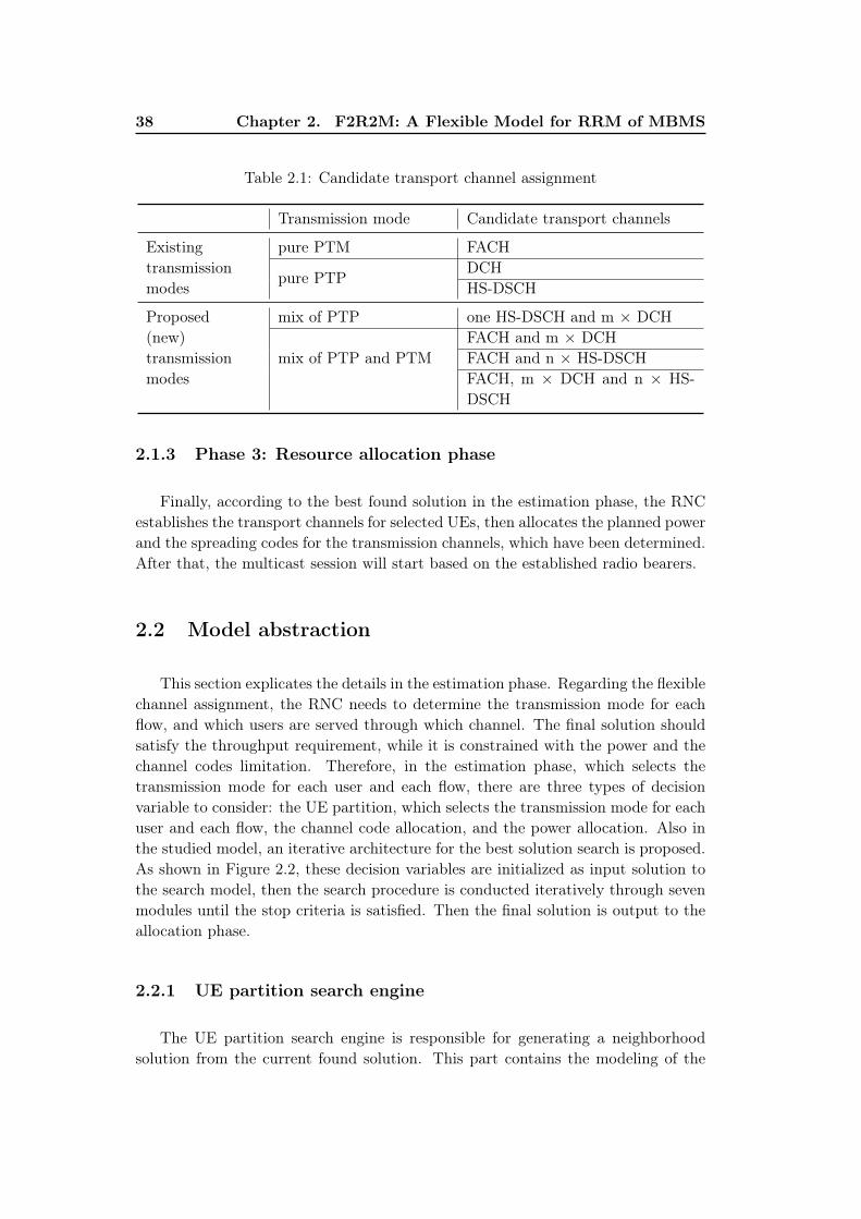
38 Chapter 2. F2R2M: A Flexible Model for RRM of MBMS
Table 2.1: Candidate transport channel assignment
Transmission mode Candidate transport channels
Existingtransmissionmodes
pure PTM FACH
pure PTPDCHHS-DSCH
Proposed(new)transmissionmodes
mix of PTP one HS-DSCH and m × DCH
mix of PTP and PTMFACH and m × DCHFACH and n × HS-DSCHFACH, m × DCH and n × HS-DSCH
2.1.3 Phase 3: Resource allocation phase
Finally, according to the best found solution in the estimation phase, the RNCestablishes the transport channels for selected UEs, then allocates the planned powerand the spreading codes for the transmission channels, which have been determined.After that, the multicast session will start based on the established radio bearers.
2.2 Model abstraction
This section explicates the details in the estimation phase. Regarding the flexiblechannel assignment, the RNC needs to determine the transmission mode for eachflow, and which users are served through which channel. The final solution shouldsatisfy the throughput requirement, while it is constrained with the power and thechannel codes limitation. Therefore, in the estimation phase, which selects thetransmission mode for each user and each flow, there are three types of decisionvariable to consider: the UE partition, which selects the transmission mode for eachuser and each flow, the channel code allocation, and the power allocation. Also inthe studied model, an iterative architecture for the best solution search is proposed.As shown in Figure 2.2, these decision variables are initialized as input solution tothe search model, then the search procedure is conducted iteratively through sevenmodules until the stop criteria is satisfied. Then the final solution is output to theallocation phase.
2.2.1 UE partition search engine
The UE partition search engine is responsible for generating a neighborhoodsolution from the current found solution. This part contains the modeling of the
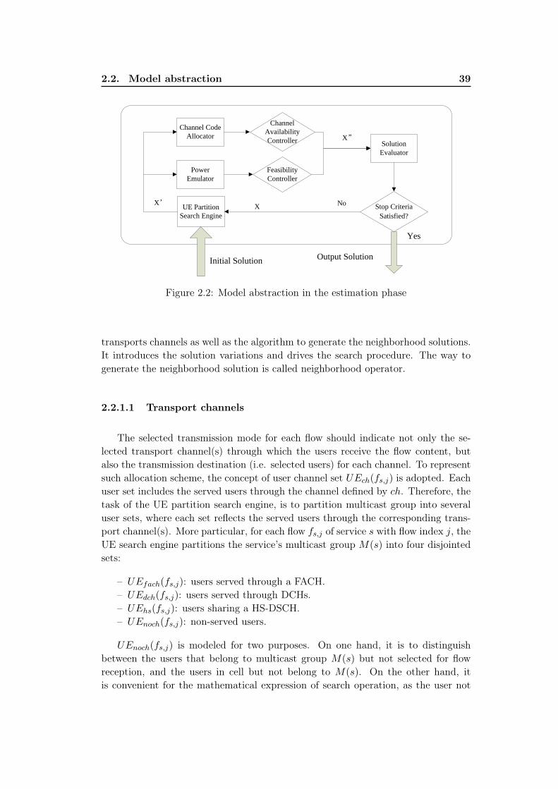
2.2. Model abstraction 39
Channel Code Allocator
SolutionEvaluator
UE PartitionSearch Engine
No
Power Emulator
FeasibilityController
XX’
Channel Availability Controller X”
Stop CriteriaSatisfied?
Output SolutionInitial Solution
Yes
Figure 2.2: Model abstraction in the estimation phase
transports channels as well as the algorithm to generate the neighborhood solutions.It introduces the solution variations and drives the search procedure. The way togenerate the neighborhood solution is called neighborhood operator.
2.2.1.1 Transport channels
The selected transmission mode for each flow should indicate not only the se-lected transport channel(s) through which the users receive the flow content, butalso the transmission destination (i.e. selected users) for each channel. To representsuch allocation scheme, the concept of user channel set UEch(fs,j) is adopted. Eachuser set includes the served users through the channel defined by ch. Therefore, thetask of the UE partition search engine, is to partition multicast group into severaluser sets, where each set reflects the served users through the corresponding trans-port channel(s). More particular, for each flow fs,j of service s with flow index j, theUE search engine partitions the service’s multicast group M(s) into four disjointedsets:
– UEfach(fs,j): users served through a FACH.– UEdch(fs,j): users served through DCHs.– UEhs(fs,j): users sharing a HS-DSCH.– UEnoch(fs,j): non-served users.
UEnoch(fs,j) is modeled for two purposes. On one hand, it is to distinguishbetween the users that belong to multicast group M(s) but not selected for flowreception, and the users in cell but not belong to M(s). On the other hand, itis convenient for the mathematical expression of search operation, as the user not

40 Chapter 2. F2R2M: A Flexible Model for RRM of MBMS
selected for flow reception is also a part of the radio resource assignment solution.For UEch(fs,j) with ch ∈ fach, dch, hs, an empty user set means this channel isnot selected for flow transmission. If fs,j is not selected for transmission, then itssubscribed users are all moved into the set of UEnoch(fs,j). This operation generallyonly happens for advanced flow solution operation.
To guarantee the service coverage, two basic principles are defined. First, allusers in multicast group should be selected to receive fs,0 or fs,1. This principle isdefined as a constraint in Equation 2.1a. In Equation 2.1b, R(fs,j) represents theusers who are receiving fs,j . The principle defined in Equation 2.1c restricts thatthe advanced flow is only sent to users who also receive the lower level flow, that isto avoid the redundant content transfer to the same user.
∀s, j ∈ 0, 1, R(fs,j) = M(s) (2.1a)
R(fs,j) = UEfach(fs,j) ∪ UEdch(fs,j) ∪ UEhs(fs,j) (2.1b)
∀s, j ≥ 2, R(fs,j) ⊆ R(fs,j−1) (2.1c)
Moreover, the user partition for fs,j should be in accord with the channel char-acteristics. If di is the distance of the user ti from the base station, and dthr is thedistance threshold found during the optimization procedure, other constraints aredefined in Equation 2.2.
∀ti ∈ UEfach, di ≤ dthr (2.2a)
∀tj ∈ UEdch ∪ UEhs ∪ UEnoch, dj > dthr (2.2b)
∀chm, chn ∈ fach, dch, hs, noch, UEchm ∩ UEchn = φ (2.2c)
The constraint in Equation 2.2a is to guarantee that UEfach(fs,j) includes theclosest users in the multicast group. That is because FACH is a common channeland can be listened by all users within its coverage. The constraint in Equation 2.2bmeans that the users in multicast group, farther than the FACH coverage, are as-signed to HS-DSCH or DCH. When there is no available channel code for a givenuser, this user is switched to UEnoch(fs,j). The constraint in Equation 2.2c guaran-tees that the user sets for each flow do not overlap as sending the same flow to thesame user through more than one channel will waste resource.
In the proposed model, the user partition is initialized randomly or by predefinedmethod, and then is modified during each iteration of the optimization procedure.The modification strategies will be described in the next section.
2.2.1.2 Neighborhood Operators
As shown in Figure 2.2, at each iteration, the UE partition search engine isapplied to a new search partition. This search is done through a neighborhood

2.2. Model abstraction 41
operation function which moves the current solution x into a neighbor solution x′.The neighborhood operator is the key element that leads to different optimizationperformance. In this section, two neighborhood operators are proposed, which definetwo associated neighborhood structures.
Single insert operator. The single insert operator δSI moves only one userfrom an initial channel cho to a target channel chi for each operator application. Itrandomly selects a user tj and moves it from UEcho to UEchi
. If FACH is one ofthe channel cho or chi, then tj is determined by the following principles:
– From FACH: tj is the farthest user within UEfach, i.e. it reduces the FACHcoverage as well as its power consumption.
– To FACH: tj is the nearest user within UEhs or UEdch or UEnoch, i.e. itminimizes the additional power consumption for FACH.
The δSI operation is implemented through the following three steps:1. Choose randomly one channel set cho, UEcho 6= φ, UEcho is the “output” user
set.2. Select randomly another channel set UEchi
as the “input” user set, chi 6= cho.3. Select randomly user tj from UEcho , δSI moves tj from UEcho to UEchi
.
Table 2.2: Single insert operation example
Solution UEfach UEdch UEhs UEnoch
x1 t1, t2, t3 t4, t5, t7, t8 t6, t9 t10, t11
x2 t1, t2 t3, t4, t5, t7, t8 t6, t9 t10, t11
x3 t1 t2, t3, t4, t5, t7, t8 t6:, t9 t10, t11
x4 t1 t2, t3, t4, t5, t6:, t7, t8 t9 t10, t11
Table 2.2 shows the example of δSI operations, which transfer solution x1 to x4.The first column lists the solution name, each row illustrates the UE partitions forone solution. The four channel user sets in the corresponding solution are listedfrom the second to the fifth columns. Therefore each table cell shows the terminalsin one user channel set. The terminal index is arranged in ascending order of thedistance from the Node B, e.g. the smaller index represents the closer user distance.To move the solution x1 to x4, three steps of single insert operator are performed:
– Move 1: x1 → x2, cho = FACH, chi = DCH. The farthest user t3 in UEfach
is moved to UEdch.– Move 2: x2 → x3, cho = FACH, chi = DCH. The farthest user t2 in UEfach
is moved to UEdch.
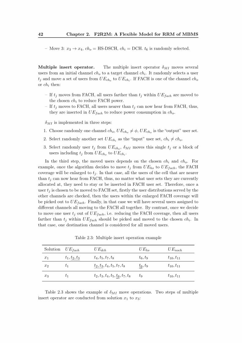
42 Chapter 2. F2R2M: A Flexible Model for RRM of MBMS
– Move 3: x3 → x4, cho = HS-DSCH, chi = DCH. t6 is randomly selected.
Multiple insert operator. The multiple insert operator δMI moves severalusers from an initial channel cho to a target channel chi. It randomly selects a usertj and move a set of users from UEcho to UEchi
. If FACH is one of the channel choor chi then:
– If tj moves from FACH, all users farther than tj within UEfach are moved tothe chosen chi to reduce FACH power.
– If tj moves to FACH, all users nearer than tj can now hear from FACH, thus,they are inserted in UEfach to reduce power consumption in cho.
δMI is implemented in three steps:
1. Choose randomly one channel cho, UEcho 6= φ, UEcho is the “output” user set.
2. Select randomly another set UEchias the “input” user set, chi 6= cho.
3. Select randomly user tj from UEcho , δMI moves this single tj or a block ofusers including tj from UEcho to UEchi
.
In the third step, the moved users depends on the chosen chi and cho. Forexample, once the algorithm decides to move tj from UEhs to UEfach, the FACHcoverage will be enlarged to tj . In that case, all the users of the cell that are nearerthan tj can now hear from FACH, thus, no matter what user sets they are currentlyallocated at, they need to stay or be inserted in FACH user set. Therefore, once auser tj is chosen to be moved to FACH set, firstly the user distributions served by theother channels are checked, then the users within the enlarged FACH coverage willbe picked out to UEfach. Finally, in that case we will have several users assigned todifferent channels all moving to the FACH all together. By contrast, once we decideto move one user tj out of UEfach, i.e. reducing the FACH coverage, then all usersfarther than tj within UEfach should be picked and moved to the chosen chi. Inthat case, one destination channel is considered for all moved users.
Table 2.3: Multiple insert operation example
Solution UEfach UEdch UEhs UEnoch
x1 t1, t2, t3 t4, t5, t7, t8 t6, t9 t10, t11
x2 t1 t2, t3, t4, t5, t7, t8 t6, t9 t10, t11
x3 t1 t2, t3, t4, t5, t6, t7, t8 t9 t10, t11
Table 2.3 shows the example of δMI move operations. Two steps of multipleinsert operator are conducted from solution x1 to x3:

2.2. Model abstraction 43
– Move 1: x1 → x2, cho = FACH, chi = DCH, tj = t2. Supposing that FACHcoverage is reduced, t3 is farther than t2 from the base station, then both t2and t3 are moved to DCH user set.
– Move 2: x2 → x3, cho = HS-DSCH, chi = DCH, tj = t6. t6 is ordered beforet7 as it is closer to the Node B than t7.
By comparing with the example in Table 2.2, it is shown that δMI operatorneeds less operations than δSI to move the users, then there are two neighborhoodstructures as a Variable Neighborhood Search (VNS) algorithm.
2.2.2 Channel code allocator and availability control
When the UE partition search engine determines the user selection and thechannel assignment, the channel code allocator then assigns available downlink or-thogonal codes to nonempty user sets. The channelization codes are picked from theOrthogonal Variable Spreading Factor (OVSF) code tree (see Figure 1.5). The allo-cation procedure corresponds to the orthogonal principle of OVSF codes [6]: if onecode on the OVSF tree is used, all codes underneath it are no longer usable. Hencethe channel code with proper spreading factor should be selected according to theusers in UEch(fs,j), the requested flows bandwidth, and the occupation situation ofOVSF code tree.
The use of OVSF codes allows the orthogonality between different spreadingcodes. We define CH(fs,j , t) to represent the channelization code allocated to usert for the receiving flow fs,j . The selection of CH(fs,j , t) is related with the datarate of fs,j . On one hand, the allocated channel bandwidth should be not higherthan the flow bandwidth; this is to avoid unnecessary radio resource waste. On theother hand, the channel code allocator uses channelization codes from the branchwith the smallest spreading factor satisfying the required bandwidth.
As shown in Table 2.4, the lowest used spreading factor in UMTS FDD downlinkis SF=4, which corresponds to the raw symbol rate of 960 kbps, the channel bit rateof 1920 kbps (QPSK modulation) and the user bit rate of 768 kbps with 1/2.5 ratecoding. Full rate voice is on SF=128, meaning a maximum of 128 simultaneousvoice calls on a 5 Mhz carrier, which corresponds to the raw symbol rate of 30 kbps,the channel bit rate of 60 kbps and the user bit rate of 12.2 kbps with 1/5 ratecoding.
The channel availability controller will check if all the channel codes are availablein the OVSF code tree. If any channel code is already occupied for a given user,through a given channel, the related user will be moved to the non-served user setUEnoch(fs,j).
Let’s take the solution x1 in Table 2.3 as an example. The spreading codes will

44 Chapter 2. F2R2M: A Flexible Model for RRM of MBMS
Table 2.4: Spreading factor and downlink user bit rate in UMTS FDD [5]
Spreadingfactor
Channelsymbol rate(kbps)
QPSKchannel bitrate (kbps)
Ratecoding1/k (k)
User bit rate(kbps)
4 960 1920 2.5 768
8 480 960 2.5 384
16 240 480 3.75 128
32 120 240 3.75 64
64 60 120 3.75 32
128 30 60 5 12.2 full rate voice
256 15 30 4 7.5 half rate voice
512 7.5 15 2 7.5 half rate voice
be assigned to users in x1 to receive a flow with bandwidth of 64 kbps, with 1/3.75
rate coding. For channel bandwidth of 64 kbps, the channel spreading factor is 32(see Table 2.4). In the OVSF code tree, the root depth is 1, the channel code withSF=32 is at depth log2 32 = 5.
x1 = t1, t2, t3,︸ ︷︷ ︸UE(fach)
t4, t5, t7, t8,︸ ︷︷ ︸UE(dch)
t6, t9,︸ ︷︷ ︸UE(hs)
t10, t11︸ ︷︷ ︸UE(noch)
(2.3)
As shown in Figure 2.3, there are 32 codes in depth 5, each code is representedas C32,n, n ∈ 0, . . . , 31, where n is the code index.
The channel code allocator assigns the available channel codes to users in x1 fromthe OVSF tree through the following procedure: firstly C32,0 is assigned to the FACHbecause the UEfach in x1 is non-empty. Note that two OVSF codes are orthogonalif and only if neither code lies on the path from the other code to the root. Then thecodes C4,0, C8,0, C16,0, C64,0, C64,1, C128,0, C128,1 and so on, cannot be assigned toany other user in the same cell. Secondly, four channel codes are assigned for usersin UEdch. The codes C32,1, C32,2, C32,3 and C32,4 are then selected, each code forone dedicated channel serving one dedicated user. In consequence, the codes C16,1,C16,2 in lower depth and so on, and the codes C64,2, . . . , C64,9 in higher depth andso on, are all blocked. Thirdly, there are two users in UEhs; the total bandwidthrequirement for HS-DSCH is 64× 2 = 128 kbps. Because HS-DSCH only allocateschannel codes with SF=16, C16,3 is selected and assigned to HS-DSCH, which willbe shared by users t6 and t9. Finally, the total allocated codes for x1 are:
– C32,0 for all mobiles in UEfach
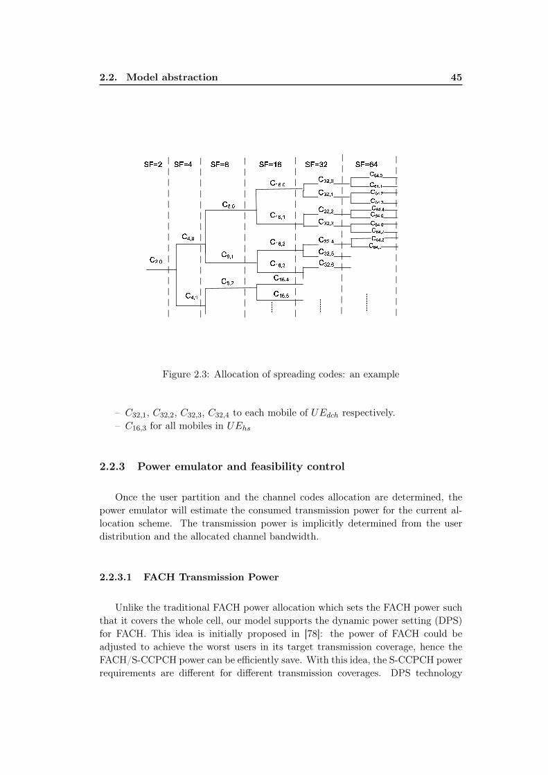
2.2. Model abstraction 45
Figure 2.3: Allocation of spreading codes: an example
– C32,1, C32,2, C32,3, C32,4 to each mobile of UEdch respectively.– C16,3 for all mobiles in UEhs
2.2.3 Power emulator and feasibility control
Once the user partition and the channel codes allocation are determined, thepower emulator will estimate the consumed transmission power for the current al-location scheme. The transmission power is implicitly determined from the userdistribution and the allocated channel bandwidth.
2.2.3.1 FACH Transmission Power
Unlike the traditional FACH power allocation which sets the FACH power suchthat it covers the whole cell, our model supports the dynamic power setting (DPS)for FACH. This idea is initially proposed in [78]: the power of FACH could beadjusted to achieve the worst users in its target transmission coverage, hence theFACH/S-CCPCH power can be efficiently save. With this idea, the S-CCPCH powerrequirements are different for different transmission coverages. DPS technology

46 Chapter 2. F2R2M: A Flexible Model for RRM of MBMS
requests to enable channel quality measurement report from UE in CELL_FACHstate, e.g. the received Common Pilot Channel (CPICH) Ec/No signal quality onUE side [78]. Based on the periodic report from UE, typically every 600 ms forCELL_FACH, the FACH power will be different depending on the various userdistributions in UEfach(fs,j).
Table 2.5: Estimated S-CCPCH power vs. cell coverage (PedestrianB 3km/h) [5]
Estimated cell coverage, % Power for 64 kbps service, W
30 0.64
40 0.8
50 1.0
60 1.2
70 1.8
80 2.8
90 4
100 10
Table 2.5 shows the simulation results in the 3GPP technical report [12]. In thisreport, the authors study the S-CCPCH power level to capture the simulation resultsin MBMS standardization [1] in which the simulated FACH power are conducted bySIEMENS private simulator presented in [32, 31]. As the dynamic power setting forFACH is not standardized in MBMS, the simulation results in [12] do not involveall geometry coverages of the cell for various service bandwidth. For example, fora 64 kbps service, 80ms TTI and 1% BLER target, the FACH transmit power issimulated with a cell coverage from 30% to 100% (see Table 2.5). While for 16, 32,128 and 256 kbps services, the results are only for the cell coverage from 90% to95%.
Besides, in our simulation setup, the cell layout is 3-cell sectorization with site-to-site distance of 3 km, i.e. the distance between two Node B. Where the Node B islocated in the corner of the three cells, thus the cell radius is 1 km and the farthestuser distance from Node B could be 2 km. While in [1] the site-to-site distance is1 km, the Node B sits in the cell center and the farthest distance between the UEand the Node B is 0.5 km. Regarding the parameter setting difference and lackingof various geometry coverages, the FACH estimated power is simulated by OPNETModeller 15.0.A [8], with the parameter setup in Table 2.6.
The obtained FACH transmission power is shown in Figure 2.4. The simulationparameter settings are Pedestrian B 3 km/h with geometry factor = - 3dB, BlockError Rate (BLER) = 1% and Transmission Time Interval (TTI) = 80ms. The

2.2. Model abstraction 47
0 500 1000 1500 20000
2
4
6
8
10
12
14
16
18
20
user distance from Node B (m)
Pow
er o
f FA
CH
(w
atts
)
PFACH
for various cell coverage, BLER=1%, PB3, 80ms TTI
32 kbps64 kbps128 kbps256 kbps
Figure 2.4: FACH transmission power obtained by OPNET 15.0.A
BLER is the error rate of the transport data passed by the physical layer to theMAC layer for a given transport channel. The TTI is the interval of time overwhich a transport data is transmitted on the radio link.
FACH is the common channel that many users can access at the same time withthe same resource (one channel code and one portion of power). Although FACH isthe favorite choice for MBMS transmission, other crucial factors such as the numberof users within the multicast group, the user distances from the serving Node B,the service bandwidth, the throughput requirement and the Eb/No target affect thechoice of the most efficient transport channel.
2.2.3.2 DCH Transmission Power
On the PTP downlink transmissions, where the multiple DCHs are used, fastpower control is used to maintain the quality of each link (set target Eb/No = 3
dB in our simulation [53]) and to provide a reliable connection for the receiver toobtain data with acceptable error rate. Besides, DCH power control supports tomaintain required link quality with just enough power thus to ensure the minimuminterference.
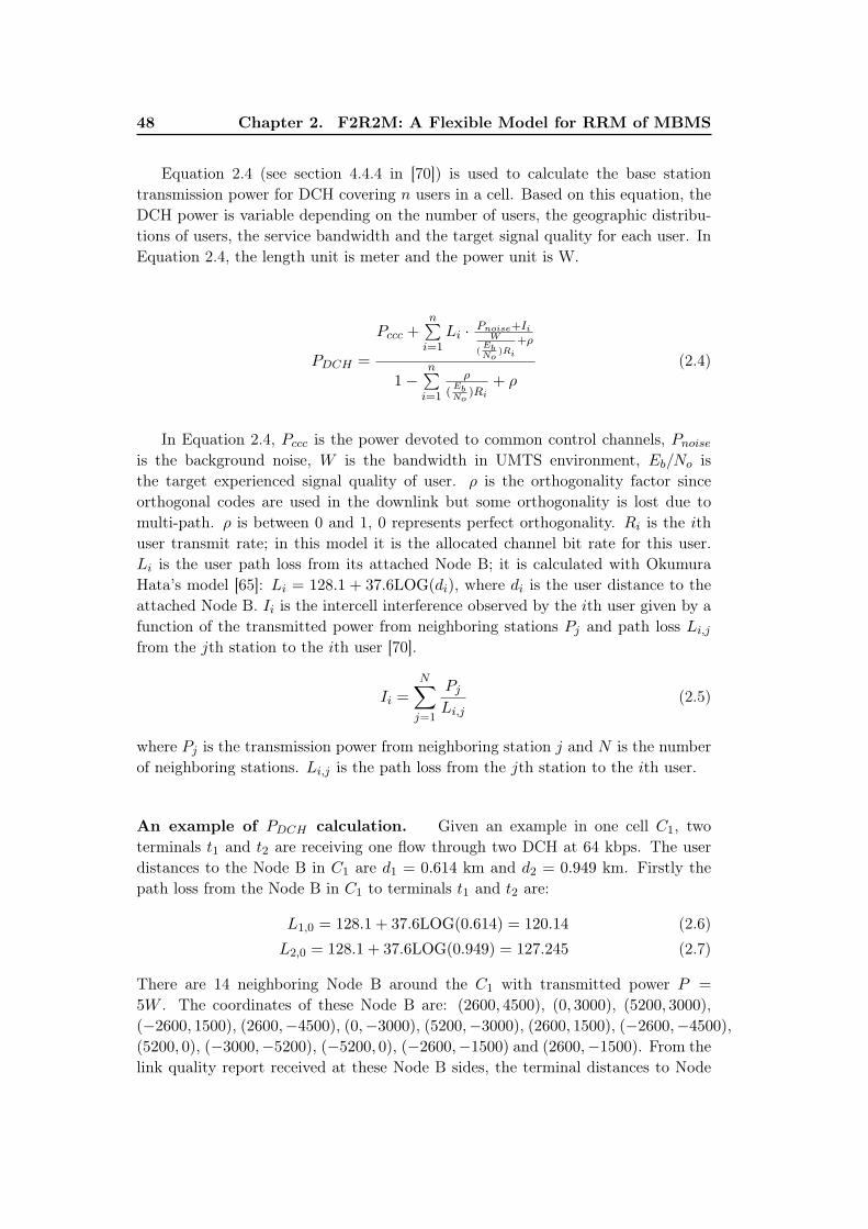
48 Chapter 2. F2R2M: A Flexible Model for RRM of MBMS
Equation 2.4 (see section 4.4.4 in [70]) is used to calculate the base stationtransmission power for DCH covering n users in a cell. Based on this equation, theDCH power is variable depending on the number of users, the geographic distribu-tions of users, the service bandwidth and the target signal quality for each user. InEquation 2.4, the length unit is meter and the power unit is W.
PDCH =
Pccc +n∑
i=1Li · Pnoise+Ii
W
(EbNo
)Ri
+ρ
1−n∑
i=1
ρ
(EbNo
)Ri
+ ρ
(2.4)
In Equation 2.4, Pccc is the power devoted to common control channels, Pnoise
is the background noise, W is the bandwidth in UMTS environment, Eb/No isthe target experienced signal quality of user. ρ is the orthogonality factor sinceorthogonal codes are used in the downlink but some orthogonality is lost due tomulti-path. ρ is between 0 and 1, 0 represents perfect orthogonality. Ri is the ithuser transmit rate; in this model it is the allocated channel bit rate for this user.Li is the user path loss from its attached Node B; it is calculated with OkumuraHata’s model [65]: Li = 128.1 + 37.6LOG(di), where di is the user distance to theattached Node B. Ii is the intercell interference observed by the ith user given by afunction of the transmitted power from neighboring stations Pj and path loss Li,j
from the jth station to the ith user [70].
Ii =
N∑j=1
Pj
Li,j(2.5)
where Pj is the transmission power from neighboring station j and N is the numberof neighboring stations. Li,j is the path loss from the jth station to the ith user.
An example of PDCH calculation. Given an example in one cell C1, twoterminals t1 and t2 are receiving one flow through two DCH at 64 kbps. The userdistances to the Node B in C1 are d1 = 0.614 km and d2 = 0.949 km. Firstly thepath loss from the Node B in C1 to terminals t1 and t2 are:
L1,0 = 128.1 + 37.6LOG(0.614) = 120.14 (2.6)
L2,0 = 128.1 + 37.6LOG(0.949) = 127.245 (2.7)
There are 14 neighboring Node B around the C1 with transmitted power P =
5W . The coordinates of these Node B are: (2600, 4500), (0, 3000), (5200, 3000),(−2600, 1500), (2600,−4500), (0,−3000), (5200,−3000), (2600, 1500), (−2600,−4500),(5200, 0), (−3000,−5200), (−5200, 0), (−2600,−1500) and (2600,−1500). From thelink quality report received at these Node B sides, the terminal distances to Node

2.2. Model abstraction 49
B are obtained, then the neighborhood cell interference to each terminal could becalculated:
i ∈ 1, 2, Ii =14∑j=1
5
Li,j(2.8)
where L1,j is the path loss from jth neighbor cell to terminal t1. According to theparameter setting in Table 2.6, the value of PDCH for transmission to t1 and t2 iscalculated:
PDCH =
1 +2∑
i=1Li · 10−10+Ii
5×10⁶
(103/10)64000+0.5
1−2∑
i=1
0.5(103/10)64000
+ 0.5
= 0.0787W (2.9)
2.2.3.3 HS-DSCH Transmission Power
HS-DSCH is a rate controlled rather than a power controlled transport channel[49]. In HSDPA, the fast power control and variable spreading factor principles(characterizing Release 99 channels) are replaced by the link adaptation functional-ity, including techniques such as dynamic Adaptive Modulation and Coding (AMC),multicode operation, fast scheduling, Hybrid ARQ (HARQ) and short TTI of 2ms.
There are two modes to allocate the transmission power for HS-DSCH. In thefirst mode, a fixed amount of power is explicitly allocated per cell, and might beupdated any time later. In the second mode, the base station is allowed to useany unused power remaining after serving other power controlled channels (suchthose for voice and non HSDPA UE) for HS-DSCH transmission [49]. In the firstmode, setting the power too high might result in too much interference in cell, whilesetting it too low could not achieve the highest data rate. Therefore, in our work,like in most of the real networks, the second mode is considered to provide only therequired amount of power so as to satisfy the MBMS multicast users. Equation 2.10is used to calculate the minimum required HS-DSCH transmission power to achievea minimum required HS-DSCH data rate at the edge of channel coverage [49].
PHS−DSCH = SINRhs × [ρ−G−1]Pintra
SF16(2.10)
Where ρ is the orthogonality factor. SF16 is the spreading factor equal to 16, asthe allocation of HS-DSCH is in units of channelization codes of length 16. Pintra
is the total power transmitted in the serving cell. G is the geometry factor orthe Carrier-to-Noise-and-Interference Ratio (C/(N + I)) defined according to the

50 Chapter 2. F2R2M: A Flexible Model for RRM of MBMS
following equation [53]:
G =Pintra
Iinter + Pnoise(2.11)
Where Iinter is the power spectral density of a band limited white noise source(simulating the interference from neighboring cells) and Pnoise is the effective powerspectral density of the Additive Gaussian White Noise (AGWN).
G is related with the user position. For a user at the cell edge, the interferingpower from the neighboring cells is higher than the transmitted power from theserving cell, thus G is expressed by a lower value. In the macrocell (hexagonallayout with 1000 m base station spacing), the user within 80% coverage experiencesa geometry factor of −2.5dB or better, that is Iinter is the double of Pintra, within95% the geometry factor is at least −5.2dB [32], that is Iinter is the triple of Pintra.
SINRhs in Equation 2.10 is the target user experienced Signal-to-Interference-plus-Noise Ratio (SINR) for any tk assigned to UEhs. Based on the analytic for-mulation driven by link-level simulation results in [11], the value of SINRhs couldbe obtained according to the Channel Quality Information (CQI) and target BLER(set 1% in this work). The CQI is obtained through the target HS-DSCH totalbandwidth and mapping table of MAC-hs bit rates versus CQI (Appendix B) [13].Then PHS−DSCH is calculated by applying SINRhs and G into Equation 2.10.
An example of PHS−DSCH calculation. Recall the example presented in sec-tion 2.2.3.2, we assume that the terminals t1 and t2 are receiving the flow 64 kbpsthrough HS-DSCH. According to the total bandwidth of HS-DSCH (128 kbps), fromthe mapping table in [13], the target CQI value is 5. Equation 2.12 shows the the-oretical transfer formulation.
BLER = (1 + 102SINRhs−1.03CQI+5.26√
3−LOG(CQI) )−10.7 (2.12)
Then the practical formula used in enhanced simulator NS2 [11] is shown in Equa-tion 2.13. The estimated SINRhs by Equation 2.13 is 2 dB with BLER fixed at1%.
SINRhs(dB) = 0.5(1.73205− LOG(CQI))(LOG(BLER−1.43 − 1.03))
+ 1.03CQI − 5.36 (2.13)
According to the simulation results in [32] and the higher distance of the twoterminals (949 meters) in a 3 km diameter cell, the geometry factor is 2.5 dB, hencethe transmission power of HS-DSCH for t1 and t2 is:
PHS−DSCH = 10SINRhs(dB)/10 × [0.5− 1
10G/10]20
16= 0.1288W (2.14)
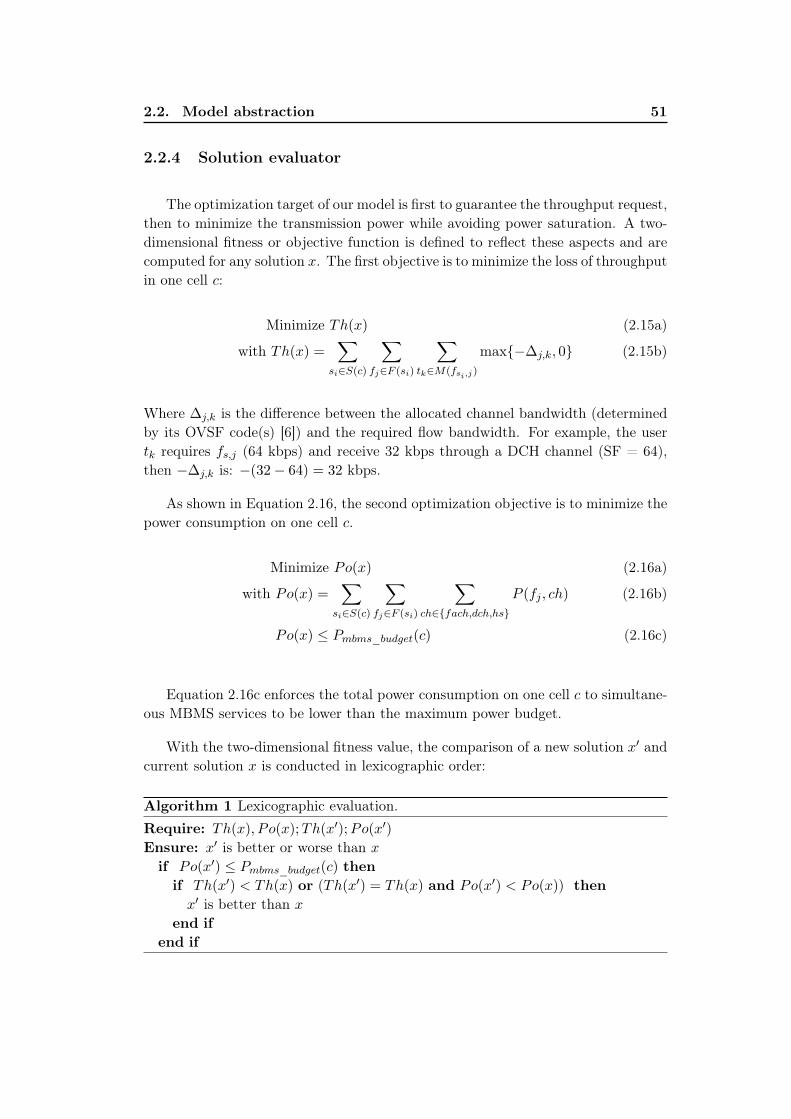
2.2. Model abstraction 51
2.2.4 Solution evaluator
The optimization target of our model is first to guarantee the throughput request,then to minimize the transmission power while avoiding power saturation. A two-dimensional fitness or objective function is defined to reflect these aspects and arecomputed for any solution x. The first objective is to minimize the loss of throughputin one cell c:
Minimize Th(x) (2.15a)
with Th(x) =∑
si∈S(c)
∑fj∈F (si)
∑tk∈M(fsi,j)
max−∆j,k, 0 (2.15b)
Where ∆j,k is the difference between the allocated channel bandwidth (determinedby its OVSF code(s) [6]) and the required flow bandwidth. For example, the usertk requires fs,j (64 kbps) and receive 32 kbps through a DCH channel (SF = 64),then −∆j,k is: −(32− 64) = 32 kbps.
As shown in Equation 2.16, the second optimization objective is to minimize thepower consumption on one cell c.
Minimize Po(x) (2.16a)
with Po(x) =∑
si∈S(c)
∑fj∈F (si)
∑ch∈fach,dch,hs
P (fj , ch) (2.16b)
Po(x) ≤ Pmbms_budget(c) (2.16c)
Equation 2.16c enforces the total power consumption on one cell c to simultane-ous MBMS services to be lower than the maximum power budget.
With the two-dimensional fitness value, the comparison of a new solution x′ andcurrent solution x is conducted in lexicographic order:
Algorithm 1 Lexicographic evaluation.Require: Th(x), Po(x);Th(x′);Po(x′)
Ensure: x′ is better or worse than x
if Po(x′) ≤ Pmbms_budget(c) thenif Th(x′) < Th(x) or (Th(x′) = Th(x) and Po(x′) < Po(x)) thenx′ is better than x
end ifend if

52 Chapter 2. F2R2M: A Flexible Model for RRM of MBMS
2.2.5 Model complexity
Let’s assume that the service si has Nf (si) flow and Nt(si) users. When the usert is receiving the flows Ft, Ft ⊆ F (si), the number of possible channel assignmentof user t is:
4 for Ft = fsi,0 or Ft = fsi,13× 4 for Ft = fsi,1, fsi,23× 3 . . . 4 for Ft = fsi,1, fsi,2 . . . fsi,Nf (si)
(2.17)
Hence, the number of allocation schemes for one user receiving service si is:
4 +
Nf (si)−1∑i=0
4 · 3i = 2(3Nf (si) + 1
), si ∈ S(c) (2.18)
The total number of possible channel assignment for all users and all services is:
Ns∏i=1
Nt(si)∏1
2(3Nf (si) + 1
)(2.19)
In Equation 2.19, Ns is the number of services, Nt(si) is the number of usersreceiving the si, Nf (si) is the number of flows in si. The number of candidatesolutions exponentially increases with the number of users, flows, and services. Bylooking at this, the exact algorithm by exhaustive search is not practical to solvethis problem, and metaheuristic approach is a reasonable choice for solving suchcombinatorial optimization problem. In chapter 3, the MBMS RRM problem willbe formally proved as NP-Hard problem.
2.2.6 Model synthesis
From subsection 2.2.1 to subsection 2.2.4, a mathematical model for the flexi-bility radio resource management for MBMS multicast service is built. Briefly, thismodel can be summarized as follows.
2.2.6.1 Input variables
The input variables of the proposed model are:
1. UE information
(a) T (c) = t1, . . . , tk. Set of mobile terminals in cell c. The terminalindexes are ordered from the closest to the farthest distance from theNode B at any time slot (after each TTI).

2.2. Model abstraction 53
(b) D(c) = d1, . . . , dk, tk ∈ T (c). Set of instantaneous distances from theNode B to the terminal, this value can be obtained through the channelquality measurement report from UE side [78].
2. Service information
(a) S(c) = s1, ..., sNs. Set of services to be transmitted to multicast groupslocated in cell c. The total number of service is Ns.
(b) F (si). The flow set of service si and its bandwidth, si ∈ S(c). F (si) =
fsi,0 if si is a single layer (SL) transmission scheme service. Or F (si) =
fsi,1, fsi,2, [fsi,3] if si is a multilayer (ML) transmission scheme service,where fsi,1 is the basic flow and fsi,j with (j > 1) are advanced flows.We assume that each service has Nf (si) flows.
(c) M(si) ⊆ T (c). Multicast group of service si. One group includes allthe terminals t1, t2, . . . , tk′ requesting the same service content withk′ ≤ k. The number of terminals in each group is Nt(si) = Nt(fsi,j),∀fsi,j ∈ F (si).
2.2.6.2 Decision variables
To support the combinational allocation modes for each flow (see Table 2.1), thedecision variables include the UE partition and the channel code assignment. TheUE partition indicates the terminals allocated in four disjointed channel user sets.
– UEfach(fs,j), users served through a FACH.– UEdch(fs,j), users served through DCHs.– UEhs(fs,j), users sharing a HS-DSCH.– UEnoch(fs,j), non-served users.
Then the channel code assignment is performed by the channel code allocator whichassigns the available channel code to a given channel.
2.2.6.3 Decision constraints
The UE partition for flow fs,j should be in accord with the channel characteris-tics, as shown in following decision constraints:
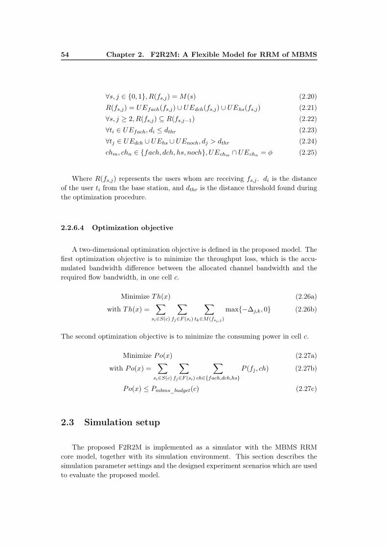
54 Chapter 2. F2R2M: A Flexible Model for RRM of MBMS
∀s, j ∈ 0, 1, R(fs,j) = M(s) (2.20)
R(fs,j) = UEfach(fs,j) ∪ UEdch(fs,j) ∪ UEhs(fs,j) (2.21)
∀s, j ≥ 2, R(fs,j) ⊆ R(fs,j−1) (2.22)
∀ti ∈ UEfach, di ≤ dthr (2.23)
∀tj ∈ UEdch ∪ UEhs ∪ UEnoch, dj > dthr (2.24)
chm, chn ∈ fach, dch, hs, noch, UEchm ∩ UEchn = φ (2.25)
Where R(fs,j) represents the users whom are receiving fs,j . di is the distanceof the user ti from the base station, and dthr is the distance threshold found duringthe optimization procedure.
2.2.6.4 Optimization objective
A two-dimensional optimization objective is defined in the proposed model. Thefirst optimization objective is to minimize the throughput loss, which is the accu-mulated bandwidth difference between the allocated channel bandwidth and therequired flow bandwidth, in one cell c.
Minimize Th(x) (2.26a)
with Th(x) =∑
si∈S(c)
∑fj∈F (si)
∑tk∈M(fsi,j)
max−∆j,k, 0 (2.26b)
The second optimization objective is to minimize the consuming power in cell c.
Minimize Po(x) (2.27a)
with Po(x) =∑
si∈S(c)
∑fj∈F (si)
∑ch∈fach,dch,hs
P (fj , ch) (2.27b)
Po(x) ≤ Pmbms_budget(c) (2.27c)
2.3 Simulation setup
The proposed F2R2M is implemented as a simulator with the MBMS RRMcore model, together with its simulation environment. This section describes thesimulation parameter settings and the designed experiment scenarios which are usedto evaluate the proposed model.

2.3. Simulation setup 55
2.3.1 Simulation parameters
Figure 2.5 depicts the macrocell layout which consists of 19 hexagonal cells.The red rings indicate the location of the Node B. The simulation focus on MBMStransmission in cell C1, assuming that only multicast services are transmitted inthis cell.
Node B
C1
C2
C3
C4
C10
C5 C17
C15
C9
C18
C19
C14 C16
C13
C12
C11
C6
C7
C8
19 Hexagon Cells, 9 3−sector base stationssite distance = 3 km, cell radius = 1 km
Figure 2.5: Cellular layout in simulation setup
Table 2.6 lists the simulation parameters. The maximum power for MBMS inone cell is 19 W, which is the total transmission power (20 W) minus the powerfor common channel (1 W); it is the conventional power setup for MBMS study[24, 28, 12]. In macrocell environment, the Okumura Hata path loss model is appliedto calculate the path loss Li of user ti, with a carrier frequency of 5 MHz and abase station antenna hight of 15 meters, that is: Li = 128.1 + 37.6LOG(di), wheredi represents the distance from the Node B to the UE in km [2].
2.3.2 Simulation scenarios
As shown in Table 2.7, a number of scenarios are designed with different ser-vice requests and user distributions. These scenarios will be used in the followingchapters for model analysis and algorithm evaluation.
The scenario name indicates the number of service s, the total number of usersu and the service transmission scheme, where S stands for scalable transmissionscheme and N stands for non-scalable transmission scheme. For example, the sce-nario 2s20uSN has two multicast services s1 and s2, both having 10 users. s1 is ascalable transmission scheme service. It consists of three flows: the basic flow fs1,1with the bandwidth 32 kbps, and the two advanced flows fs1,2 and fs1,3 with 32kbps and 64 kbps, respectively. s2 is a non-scalable transmission scheme service, i.e.

56 Chapter 2. F2R2M: A Flexible Model for RRM of MBMS
Table 2.6: System level parameter setting
Parameters Value
Cellular layout 19 hexagonal cells, 3-sector sites
Number of neighboring cells 18
Orthogonally factor (ρ) 0.5
UMTS bandwidth 5 MHz
Site to site distance 3 km
Cell radius 1 km
Base station transmit power 43 dBm (20 Watts[49] )
Background noise -100 dBm
Power of neighbor cell 37 dBm (5 Watts)
Propagation models Okumura Hata
IUT path loss environment Pedestrian B, 3 km/h
Common channel power 30 dBm (1 Watt)
Target Eb/No 3 dB
Block Error Ratio (BLER) 1 %
one flow fs2,0 with the bandwidth 128 kbps. The total bandwidth requirement of2s20uSN is 2560 kbps, obtained by 10× (32 + 32 + 64) + 10× 128.
2.3.3 Power simulation of three transport channels
In this section, to validate the power emulator in our model, simulation is con-ducted to synthesize the power consumption of three transport channels, for variousservice bandwidths. For each service bandwidth, three types of user distributions(depending on their distance to the Node B) are defined. They are named as “close”,“median” and “far”, in which, the users are randomly generated in cell C1, locatedwith random distance in given ranges: ]0, 700], ]700, 1400] and ]1400, 2000] metersfrom the Node B.
Figure 2.6 shows an example of users located in C1. There are 12 users, markedas black points, close to the Node B, the blue plus signs represent 12 users in medianlocations, and the 12 red asterisks are the users which are far from the Node B, someof them are in the cell edge.
The power simulation is conducted as follows. Assume that all users belong to

2.3. Simulation setup 57
Table 2.7: Experimental scenarios
Scenarioname
Flows of service Usernumber
Total trafficrequirement(kbps)
1s30uS s1 (f1: 64 kbps, f2: 64 kbps) 30 3840
1s60uS s1 (f1: 64 kbps, f2: 64 kbps) 60 7680
1s150uS s1 (f1: 64 kbps, f2: 64 kbps) 150 19200
2s20uSNs1 (f1: 32 kbps, f2: 32 kbps, f3: 64kbps) 10
2560s2 (f0: 128 kbps) 10
2s20uSSs1 (f1: 32 kbps, f2: 32 kbps, f3: 64kbps) 10
2560s2 (f1: 64 kbps, f2: 64 kbps) 10
2s50uSNs1 (f1: 32 kbps, f2: 32 kbps, f3: 64kbps) 30
6400s2 (f0: 128 kbps) 20
2s50uSSs1 (f1: 32 kbps, f2: 32 kbps, f3: 64kbps) 30
6400s2 (f1: 64 kbps, f2: 64 kbps) 20
3s30uSNNs1 (f1: 32 kbps, f2: 32 kbps, f3: 64kbps) 10
3200s2 (f0: 128 kbps) 10s3 (f0: 64 kbps) 10
3s30uSSNs1 (f1: 32 kbps, f2: 32 kbps, f3: 64kbps) 10
3200s2 (f1: 64 kbps, f2: 64 kbps) 10s3 (f0: 64 kbps) 10
3s50uSNNs1 (f1: 32 kbps, f2: 32 kbps, f3: 64kbps) 10
4480s2 (f1: 128 kbps) 20s3 (f0: 64 kbps) 10
3s50uSSNs1 (f1: 32 kbps, f2: 32 kbps, f3: 64kbps) 10
4480s2 (f1: 64 kbps, f2: 64kbps) 20s3 (f0: 64 kbps) 10
3s80uSNNs1 (f1: 32 kbps, f2: 32 kbps, f3: 64kbps) 30
8960s2 (f0: 128 kbps) 30s3 (f0: 64 kbps) 20
3s80uSSNs1 (f1: 32 kbps, f2: 32 kbps, f3: 64kbps) 30
8960s2 (f1: 64 kbps, f2: 64kbps) 30s3 (f0: 64 kbps) 20
3s100uSNNs1 (f1: 32 kbps, f2: 32 kbps, f3: 64kbps) 30
10240s2 (f0: 128 kbps) 40s3 (f0: 64 kbps) 30
3s100uSSNs1 (f1: 32 kbps, f2: 32 kbps, f3: 64kbps) 30
10240s2 (f1: 64 kbps, f2: 64kbps) 40s3 (f0: 64 kbps) 30

58 Chapter 2. F2R2M: A Flexible Model for RRM of MBMS
−1 −0.5 0 0.5 1 1.5 2−1
−0.5
0
0.5
1
1.5
2
2.5
Node B
C1
C2
C3
C4
C5
C6
Node B distance = 3000 m, cell radius = 1000 mUser distributions: near/median/far
Figure 2.6: Three user distributions for power comparison
the same multicast group, for a given service bandwidth and a given user distri-bution, three transport channels (i.e. FACH, HS-DSCH and DCH) are separatelyapplied in three different runs, hence there is no channel co-existing for the sameservice. The service bandwidth could be 32, 64, 128 and 256 kbps, respectively.The user distribution could be “close”, “median” or “far”; each distribution has 1to 18 users. There is no optimization in these evaluations; we run the differentscenarios separately to calculate the impact of the different parameters on MBMSperformance: user location, service bandwidth and transport channels.
Figure 2.7 shows the transmission power of the three transport channels forsending 32 kbps and 64 kbps services to users located close, median and far fromthe Node B. The x-axis shows the number of users from 1 to 18, while the y-axisplots the power level of three channels separately. When the users are close to theNode B, for 32 kbps service, DCH consumes the lowest power, while FACH poweris fixed around 1 W; it is sufficient to cover the farthest user in the multicast group.When users are in the middle of the cell, HS-DSCH offers a better power adaptationthan the other two channels. When the users are far from Node B, the transmissionpower of these channels fluctuates. For 32 kbps service, HS-DSCH consumes thelowest power when the number of users is smaller than 11 (Figure 2.7(e)), whileFACH consumes the lowest power for user number larger than 11. For 64 kbpsservice, HS-DSCH always consumes lower power than FACH and DCH whateverthe number of users is (Figure 2.7(f)). In these six runs, all required bandwidthsare satisfied.

2.3. Simulation setup 59
0 2 4 6 8 10 12 14 16 180
1
2
3
4
5
6
7
8
9
10
Number of Users
Pow
er in
Wat
ts
service bandwidth = 32 Kbps, User distribution: Near
DCH Tx PowerHS−DSCH Tx PowerFACH Tx Power
(a) 32kbps Close
0 2 4 6 8 10 12 14 16 180
2
4
6
8
10
12
14
16
18
20
Number of Users
Pow
er in
Wat
ts
service bandwidth = 64 Kbps, User distribution: Near
DCH Tx PowerHS−DSCH Tx PowerFACH Tx Power
(b) 64kbps Close
0 2 4 6 8 10 12 14 16 180
1
2
3
4
5
6
7
8
9
10
Number of Users
Pow
er in
Wat
ts
service bandwidth = 32 Kbps, User distribution: Median
DCH Tx PowerHS−DSCH Tx PowerFACH Tx Power
(c) 32kbps Median
0 2 4 6 8 10 12 14 16 180
2
4
6
8
10
12
14
16
18
20
Number of Users
Pow
er in
Wat
tsservice bandwidth = 64 Kbps, User distribution: Median
DCH Tx PowerHS−DSCH Tx PowerFACH Tx Power
(d) 64kbps Median
0 2 4 6 8 10 12 14 16 180
1
2
3
4
5
6
7
8
9
10
Number of Users
Pow
er in
Wat
ts
service bandwidth = 32 Kbps, User distribution: Far
DCH Tx PowerHS−DSCH Tx PowerFACH Tx Power
(e) 32kbps Far
0 2 4 6 8 10 12 14 16 180
2
4
6
8
10
12
14
16
18
20
Number of Users
Pow
er in
Wat
ts
service bandwidth = 64 Kbps, User distribution: Far
DCH Tx PowerHS−DSCH Tx PowerFACH Tx Power
(f) 64kbps Far
Figure 2.7: Separate power consumption of the three channels for 32 kbps and 64kbps services

60 Chapter 2. F2R2M: A Flexible Model for RRM of MBMS
0 2 4 6 8 10 12 14 16 180
2
4
6
8
10
12
14
16
18
20
Number of Users
Pow
er in
Wat
ts
service bandwidth = 128 Kbps, User distribution: Near
DCH Tx PowerHS−DSCH Tx PowerFACH Tx Power
(a) 128kbps Close
0 2 4 6 8 10 12 14 16 180
5
10
15
20
25
30
Number of Users
Pow
er in
Wat
ts
service bandwidth = 256 Kbps, User distribution: Near
DCH Tx PowerHS−DSCH Tx PowerFACH Tx Power
(b) 256kbps Close
0 2 4 6 8 10 12 14 16 180
2
4
6
8
10
12
14
16
18
20
Number of Users
Pow
er in
Wat
ts
service bandwidth = 128 Kbps, User distribution: Median
DCH Tx PowerHS−DSCH Tx PowerFACH Tx Power
(c) 128kbps Median
0 2 4 6 8 10 12 14 16 180
5
10
15
20
25
30
Number of Users
Pow
er in
Wat
ts
service bandwidth = 256 Kbps, User distribution: Median
DCH Tx PowerHS−DSCH Tx PowerFACH Tx Power
(d) 256kbps Median
0 2 4 6 8 10 12 14 16 180
2
4
6
8
10
12
14
16
18
20
Number of Users
Pow
er in
Wat
ts
service bandwidth = 128 Kbps, User distribution: Far
DCH Tx PowerHS−DSCH Tx PowerFACH Tx Power
(e) 128kbps Far
0 2 4 6 8 10 12 14 16 180
5
10
15
20
25
30
Number of Users
Pow
er in
Wat
ts
service bandwidth = 256 Kbps, User distribution: Far
DCH Tx PowerHS−DSCH Tx PowerFACH Tx Power
(f) 256kbps Far
Figure 2.8: Separate power consumption of three channels for 128 kbps and 256kbps services

2.4. Synthesis 61
Figure 2.8 shows the power emulation of the three transport channels for theservice 128 kbps and 256 kbps. It can be observed that the power consumptionincrease with the number of users and the user distance from the Node B andsometimes the total power consumption overpasses the maximum power set to 19W (Figure 2.8(b), 2.8(d), 2.8(e) and 2.8(f)).
Then two conclusions can be obtained. First, none of these three channel gainsabsolute transmission efficiency in terms of power consumption when the users num-bers and users positions are different. In this study, the user positions are randomlychanged, hence the same user number and similar geographic scenario may still havedifferent power levels. Therefore, the MBMS UE counting mechanism or any trans-mission decision algorithm based on the user numbers cannot be efficient whateverthe input scenarios. Second, HS-DSCH can truly consume the lowest power forcertain scenarios in particular when the terminal distance is not close to the NodeB.
Besides, the advantages of scalable transmission can be observed. In Figure2.8(f) at 256 kbps, when the user number is over 14, the three channels consumemore than 19 W, hence achieve the power saturation within one cell. While in Figure2.8(e), for one 128 kbps stream transmission to 14 users far from Node B, the lowestpower is 6.4 W with HS-DSCH and is also acceptable for FACH. Therefore two 128kbps streams will need 12.8 W, much less than the power requirement of one 256 kbpsstream transmission with the same channel (22 W in Figure 2.8(f)). To fully takeadvantages of the transmission characteristics of the three transport channels, wepropose to integrate the scalable transmission with the combined channel selectionand transmission.
2.4 Synthesis
This chapter presents a model for the MBMS RRM problem. This model mapsthe radio resource establishment procedure for MBMS into three phases: i) collectthe input variables; ii) determine the decision variables; and iii) establish the radiobearers according to the best found solution. The second phase plays the mostimportant role for the system performance and is the focus of our model. In thisphase, the MBMS RRM is modeled as an optimization problem which tries to findthe optimum radio resource assignment for a given scenario. To solve this prob-lem, an iterative search architecture is designed to explore new solutions. In eachiteration, seven modules are invoked consecutively:
1. UE partition search engine generates a candidate solution x′ by modifyinga current solution x.
2. Channel code allocator associates available channelization code to each

62 Chapter 2. F2R2M: A Flexible Model for RRM of MBMS
assigned transport channel.
3. Channel availability controller will shift user(s) to UEnoch when there areno more available channel code for these users, thus the candidate solution ismodified regarding the limited channel code resource.
4. Power emulator estimates the transmission power of the candidate solutionafter the channel code verification.
5. Feasibility controller will pass the candidate solution if its transmissionpower is below the cell power budget, otherwise this solution will be rejectedas unfeasible solution.
6. Solution evaluator compares the candidate solution and the current solutionin lexicographic order, it accepts the new solution if it is better than the currentsolution.
7. Stop criteria determines if the search procedure should stop, then outputthe best found solution.
To better explore the solution space, two additional flexibilities are proposed.First, instead of service based channel allocation, the flow based allocation is pro-posed, which supports the scalable streaming data. Second, this model supportsthe flexible transmission mode selection. For solution representation, a solutioncontains the UE partitioning of four different channel types, as well as the channelcode allocation and the transmission power allocation. For solution evaluation, atwo-dimensional fitness function is proposed, which reflects both the allocated band-width and the consumed power of the allocation solution. Therefore, the allocationsolution is found regarding a two-dimensional objective function, while the otherMBMS radio resource allocation approaches consider the MBMS RRM as a mono-objective optimization problem. For solution updating, two neighborhood operatorsare proposed: the single insert operator δSI and the multiple insert operator δMI .The current flow solution is transfered to a new flow solution by one application ofthe operator.
The proposed F2R2M is implemented as a simulator which reflects the MBMSRRM core model, together with its simulation environment which contains theOVSF code allocator and the power emulator. A number of scenarios are alsodesigned, which will be used for algorithm performance evaluation in the next chap-ters. Besides, to verify the implemented power emulator, the channel code allocatorand the model validity, the transmission power of the three transport channels aresimulated for various service bandwidths. The simulation results show that thetransmission power fluctuates with different users number and users distributions.Hence three observations were concluded: firstly, none of these three channel gainsabsolute transmission efficiency in terms of power consumption for arbitrary scenar-ios; secondly, HS-DSCH can consume the lowest power for certain scenarios, hencethe co-existing of R5 channel and R99 channels could improve the efficiency of ra-dio resource allocation; thirdly, the adopted scalable transmission technology can

2.4. Synthesis 63
reduce the power consumption for several scenarios, and therefore proves its valuein our model.
The proposed F2R2M enables systematic analysis for MBMS RRM problem.Also it makes it possible that optimization algorithms (e.g. metaheuristic algo-rithms), can be used to solve this MBMS RRM problem. The detailed analysis andalgorithm design will be presented in the following chapters.


Chapter 3
Model Analysis
In this chapter, we conduct an in-depth analysis on the studied problem. To un-derstand the problem complexity and the solution boundaries, the work shows that,by relaxing the OVSF code constraints, the MBMS RRM problem can be approxi-mated to be a multiple-choice knapsack problem (MCKP). It gives two outcomes:first, the NP-hard proof for MBMS RRM is self-contained because MCKP is NP-hard. Second, solving MCKP will give theoretical solution bounds for MBMS RRMsolver. To understand the structure of the solution space, the landscape analysistechnique is conducted on F2R2M. In this analysis, the landscapes differentiated bytwo neighborhood operators, single insert operator and multiple insert operator, aregenerated. Then the characteristics of the studied problem are analyzed regardingthe search space and the solution distribution. Simulations show that the studiedproblem is rugged in both search spaces. Simulations also show that multiple insertoperator is better than the single insert operator for efficient search.
Contents3.1 Knapsack problem approximation . . . . . . . . . . . . . . . 66
3.1.1 Knapsack problem and its variants . . . . . . . . . . . . . . . 663.1.2 Approximating MBMS RRM as a knapsack problem . . . . . 683.1.3 Solution bound generation of F2R2M by solving MCKP . . . 76
3.2 Fitness landscape analysis . . . . . . . . . . . . . . . . . . . . 793.2.1 Introduction of fitness landscape analysis . . . . . . . . . . . 803.2.2 Solution representations . . . . . . . . . . . . . . . . . . . . . 813.2.3 Distance measurements . . . . . . . . . . . . . . . . . . . . . 823.2.4 Greedy Local Search and its application on landscape analysis 833.2.5 Experiments and results analysis . . . . . . . . . . . . . . . . 83
3.3 Synthesis . . . . . . . . . . . . . . . . . . . . . . . . . . . . . . 90
66 Chapter 3. Model Analysis
3.1 Knapsack problem approximation
In this section, the MBMS RRM problem is formulated as a variant of theknapsack problem (KP), which represents a set of integer combinatorial optimizationproblems known as NP-Hard [30, 60].
3.1.1 Knapsack problem and its variants
The knapsack problem and its variants appear in real-world applications in awide variety of fields, such as cargo systems [47] and telecommunications [81]. Manydifferent kinds of knapsack problems are found in the literature, including multi-dimensional [40], multi-objective [26], multiple-choice knapsack problems [74] andtheir combinations [64].
Classic 0-1 knapsack problem (KP). The 0-1 knapsack problem is a classicalproblem in combinatorial optimization. Suppose a hiker needs to fill a knapsackfor a trip. He has a set of items, each with a value (benefit) of vi and a weightof wi. It is common to assume that all values and weights are positive. The hikerneeds to package selected items to his knapsack to maximize the overall value inthe knapsack, while guaranteeing that the aggregated size of all selected items donot exceed the knapsack capacity constraint W . A binary decision variable xi isintroduced to model the decision process. If the i-th item is selected then xi = 1
while xi = 0 otherwise. The standard knapsack problem is given by Equation 3.1.
Maximize z =n∑
i=1
vixi (3.1a)
Subject to ∀i, xi ∈ 0, 1,n∑
i=1
wixi ≤W (3.1b)
The objective function in the standard knapsack is to maximize the sum of thevalues of the items in the knapsack, so that the sum of the weights must be lessthan the knapsack capacity.
Multi-dimensional knapsack problem (MKP). A problem may have differentcriteria to measure the solution quality, and it is not possible to select a mostimportant criterion or to combine the criteria into a single objective function. Thegoal of a Multi-dimensional Knapsack Problem (MKP), also called m-dimensionalknapsack problem, is to maximize the profit of selected items. The selected itemsshould be partitioned over a set of knapsacks contrary to the classical KP where onlyone knapsack is available. Each knapsack is characterized by a capacity representing

3.1. Knapsack problem approximation 67
the maximal total weight it can contain. Given a set of n items and a set of m
knapsacks (m ≤ n), with vi = value of item i, wi = weight of item i, Wj = capacity
of knapsack j. The decision here is not only whether to select a single item but alsoin which knapsack it is packed. Therefore, MKP consists in selecting m disjointedsubsets of items so that the total value of the selected items be maximal, and eachsubset can be assigned to a different knapsack whose capacity is no less than the totalweight of items in the subset. Formally, this problem is modeled in Equation 3.2:
Maximize z =
m∑j=1
n∑i=1
vixij (3.2a)
Subject to ∀j ∈ 1, . . . ,m,n∑
i=1
wixij ≤Wj (3.2b)
∀i ∈ 1, . . . , n,m∑j=1
xij ≤ 1 (3.2c)
∀j ∈ 1, . . . ,m, i = 1, . . . , n, xij ∈ 0, 1 (3.2d)
wi ≥ 0, vi > 0,Wj ≥ 0 (3.2e)
A binary variable xij = 1 means that the item i is selected and packed into theknapsack j, otherwise xij = 0. The constraints of the problem ensure that eachitem is selected at most once in these knapsacks. The MKP is a well-studied andstrongly NP-Hard combinatorial optimization problem occurring in many differentapplication [29].
Multi-objective m-dimensional knapsack problem (MOKP). The multi-objective optimization problem is frequently encountered in practice. This problemcan be formulated as in Equation 3.3.
Maximize Z = n∑
i=1
v1i xi, . . . ,
n∑i=1
vki xi, . . ., k = 1, . . . , t (3.3a)
Subject to ∀j ∈ 1, . . . ,m,n∑
i=1
wjixij ≤W j (3.3b)
∀i, xi ∈ 0, 1 (3.3c)
vki > 0, wji ≥ 0,W j ≥ 0 (3.3d)
In the multi-objective m-dimensional knapsack problem, each item i has t differ-ent values (v1i , . . . , vti), which are corresponding to its benefit according to differentcriteria (e.g. price, reliability). Instead of trying to compute a single optimal so-lution with maximum value, this problem targets at computing a set of feasiblesolutions covering all possible trade-offs between the different profit values. In ad-dition, each item i has m different weights, (w1
i , . . . , wmi ) corresponding to the

68 Chapter 3. Model Analysis
resources consumption (e.g. weight, volume, ...), while the knapsack is defined by m
different capacities (W 1, . . . ,Wm) representing the corresponding resources avail-ability. Therefore, the knapsack capacity must be satisfied for each of the m resourcecategories.
Multiple-choice knapsack problem (MCKP). The Multiple-Choice Knap-sack Problem is a variant of the 0-1 knapsack problem, also known as a NP-Hardproblem [74]. Given a set of n items partitioned into k sets (classes) K1, . . . ,Kk
that should be packed into a knapsack of capacity W . Each item i is associatedwith a value, vi, representing its benefit and a weight wi. The problem goal is tochoose one and only one item from each class in such manner that the sum of thevalues of selected items is maximized and the knapsack capacity W is not exceeded.The MCKP is formulated in Equation 3.4.
Maximize z =
n∑i=1
vixi (3.4a)
Subject ton∑
i=1
wixi ≤W (3.4b)
∀j ∈ 1, . . . , k,∑i∈Kj
xi = 1 (3.4c)
∀i = 1, ..., n, xi ∈ 0, 1 (3.4d)
All parameters vi, wi and W are positive integers, the classes K1, ... , Kk aremutually disjoint, nj is the size of the class Kj . The total number of items isn =
∑kj=1 nj .
3.1.2 Approximating MBMS RRM as a knapsack problem
For MBMS RRM, the main objective is to maximize the accumulation of allo-cated bandwidth over all users and all flows, then to minimize the allocated trans-mission power. And the total transmission power should be less that a predefinedvalue Pmbms_budget.
In F2R2M, when there is no channel code satisfying the required bandwidth fora given set of users, a channelization code offering lower bandwidth will be selected.In this way, the allocated bandwidth will be less than the required throughput,and is named as bandwidth fraction. Besides, the solution of a given flow, i.e.the allocation of the OVSF code, should be considered regarding the OVSF codeoccupation by the other flows.
If the studied MBMS RRM problem is approximated as KP, the channel codeorthogonality can not be simultaneously considered in the candidate solution se-

3.1. Knapsack problem approximation 69
lection for flows, because the item selection for one flow (i.e. allocation schemes)is independent to the item selection for the other flows. Moreover, the bandwidthfraction will be meaningless without considering the OVSF code occupation and thecode orthogonality.
Therefore, to map the studied problem into a KP, it is assumed that there isno channel code limitation. Once a user is selected, the required flow bandwidth isassumed fully available. The power limitation remains as the only reason for notserving a given user for a given flow. With the OVSF code constraint in mind, theprimary KP based formulation is proposed in Equation 3.5 as a MCKP.
MaximizeNf∑j=1
nj∑i=1
vijxij (3.5a)
Subject toNf∑j=1
nj∑i=1
wijxij ≤W (3.5b)
∀j ∈ 1, . . . , Nf,nj∑i=1
xij = 1 (3.5c)
∀j ∈ 1, . . . , Nf, ∀i ∈ 1, . . . , nj, xij ∈ 0, 1 (3.5d)
Where each flow fj is associated with nj items, corresponding to a class Kj .The decision variable xij = 1 means that the ith item is selected as the allocationscheme for the flow fj . In Equation 3.5a, vij is the allocated (required) channelbandwidth of the item i concerning the flow fj (while in F2R2M, the bandwidth ofallocation solution is determined by the spreading factor of allocated channel code).In Equation 3.5b, the weight of the i-th item in the j-th class, wij , is the powerconsumption of the i-th item for flow fj . Besides, the total power consumptionshould be less than W , which is the value of Pmbms_budget. xij is a binary decisionvariable, xij = 1 when the i-th item in the j-th class is packed into the knapsack,otherwise xij = 0. The objective function in Equation 3.5 is to maximize the sumof the values selected, such that the sum of the weights must be less than W .
Equation 3.5 gives the hints that, by relaxing the OVSF code constraints, thestudied problem may possibly be formulated as a MCKP, where each class is a set ofcandidate items for a given flow, each item represents a possible partition of its usersamong DCH served users, HS-DCH served users, FACH served users and not servedusers. The optimization target is to choose one and only one item from each class(Equation 3.5c), to maximize the allocated bandwidth (Equation 3.5a) and satisfythe power limitation (Equation 3.5b). However, more formulation details need tobe specified:
– The representation of the knapsack: the knapsack could represent a transport

70 Chapter 3. Model Analysis
channel, a type of transmission mode or a whole cell.– The item representation: an item could represent an allocation scheme for the
services, or for the flows, or for a given user.– The calculations of vij and wij which depend on the item structure.
To address these issues, three candidate propositions are discussed later.
3.1.2.1 Proposition 1: multi-dimensional MCKP
In Equation 3.5, in a given class associated with a given flow, an item could rep-resent a user for the flow reception. In order to distinguish which channel serves theuser (i.e. which channel set the user belongs to), instead of one knapsack with capac-ity of Pmbms_budget (Equation 3.5b), three knapsacks are defined, each represents atransport channel. Therefore, in this proposition, the flexible MBMS RRM problemis proposed to be formulated as the Multi-dimensional Multiple-Choice KnapsackProblem (MMKP).
As defined in the multi-dimensional KP, each knapsack is characterized by acapacity representing the maximal weight it can contain. Each item has m types ofweight, and each weight measures the solution quality knowing that each weight isa constant value in the corresponding knapsack.
Based on the problem characteristic, in this proposition, the knapsack capacitycould represent either the maximal bandwidth for each channel, or the maximalpower for each channel.
1. MMKP with three knapsacks. Each knapsack represents one of the threetransport channels: FACH, DCH and HS-DSCH. The knapsack capacity isthe power limitation for each of these channels.
2. MMKP with four knapsacks. One knapsack represents the total power lim-itation in the whole cell. The capacity of the other three knapsacks is themaximal bandwidth offered by the channel category.
In the first assumption, the weights (power) of item for different knapsacks (chan-nel) are different. Equation 3.6 shows the calculation of the total weight of theselected items packed in each knapsack (channel), which is the transmission power
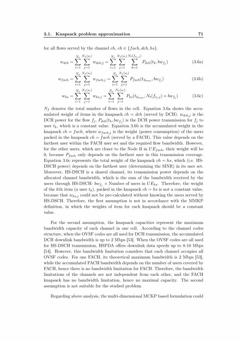
3.1. Knapsack problem approximation 71
for all flows served by the channel ch, ch ∈ fach, dch, hs.
wdch =
Ns∑i=1
Nf (si)∑j=1
wdch,j =
Ns∑i=1
Nf (si)∑j=1
Nt(fsi,j)∑k=1
Pdch(tk, bwfj ) (3.6a)
wfach =
Ns∑i=1
Nf (si)∑j=1
wfach,j =
Ns∑i=1
Nf (si)∑j=1
Pfach(tdmax , bwfj ) (3.6b)
whs =
Ns∑i=1
Nf (si)∑j=1
whs,j =
Ns∑i=1
Nf (si)∑j=1
Phs(tdmax , Nt(fsi,j)× bwfj ) (3.6c)
Nf denotes the total number of flows in the cell. Equation 3.6a shows the accu-mulated weight of items in the knapsack ch = dch (served by DCH). wdch,j is theDCH power for the flow fj , Pdch(tk, bwfj ) is the DCH power transmission for fj touser tk, which is a constant value. Equation 3.6b is the accumulated weight in theknapsack ch = fach, where wfach,j is the weight (power consumption) of the userspacked in the knapsack ch = fach (served by a FACH). This value depends on thefarthest user within the FACH user set and the required flow bandwidth. However,for the other users, which are closer to the Node B in UEfach, their weight will be0, because Pfach only depends on the farthest user in this transmission coverage.Equation 3.6c represents the total weight of the knapsack ch = hs, which (i.e. HS-DSCH power) depends on the farthest user (determining the SINR) in its user set.Moreover, HS-DSCH is a shared channel, its transmission power depends on theallocated channel bandwidth, which is the sum of the bandwidth received by theusers through HS-DSCH: bwfj × Number of users in UEhs. Therefore, the weightof the kth item (a user tk), packed in the knapsack ch = hs is not a constant value,because that whs,j could not be pre-calculated without knowing the users served byHS-DSCH. Therefore, the first assumption is not in accordance with the MMKPdefinition, in which the weights of item for each knapsack should be a constantvalue.
For the second assumption, the knapsack capacities represent the maximumbandwidth capacity of each channel in one cell. According to the channel codesstructure, when the OVSF codes are all used for DCH transmission, the accumulatedDCH downlink bandwidth is up to 2 Mbps [53]. When the OVSF codes are all usedfor HS-DSCH transmission, HSPDA offers downlink data speeds up to 8-10 Mbps[54]. However, this bandwidth limitation considers that each channel occupies allOVSF codes. For one FACH, its theoretical maximum bandwidth is 2 Mbps [53],while the accumulated FACH bandwidth depends on the number of users covered byFACH, hence there is no bandwidth limitation for FACH. Therefore, the bandwidthlimitations of the channels are not independent from each other, and the FACHknapsack has no bandwidth limitation, hence no maximal capacity. The secondassumption is not suitable for the studied problem.
Regarding above analysis, the multi-dimensional MCKP based formulation could

72 Chapter 3. Model Analysis
not be accepted.
3.1.2.2 Proposition 2: parallel MCKP
The second proposition defines a single knapsack instead of multiple knapsacks,but a set of classes are constructed associated with each flow. In these classes, eachitem describes how the transmission modes are allocated for users receiving a givenflow: users served by FACH, users served by DCH, users served by HS-DSCH or notserved users. Therefore, the second proposition formulates the problem as MCKP.More precisely, each item associated with a given flow, represents a set of users orone user:
1. A set of user served by FACH receiving the same flow or not served.
2. One user served by DCH, HS-DSCH or not served.
The first case leads to one item which includes the users whose distance fromthe base station do not exceeds the threshold dthr. In the second case, an itemrefers to one user which is allocated to DCH, HS-DSCH, or not served. Itemsindicating the same set of terminals for the same flow reception constitute one class.With this proposition, the value/profit of each item could be calculated in advance.Equation 3.7 describes a simple scenario to illustrate the second proposition.
A simple scenario:
S(c) = s1 (3.7a)
F (s1) = f1, f2 (3.7b)
M(s1) = t1, t2, t3 (3.7c)
Where M(s1) is a set of terminals belongs to the multicast group of service s1,which has Nf = 2 flows. The requested flow bandwidth are both 64 kbps. In themulticast group Ms1 of service s1, three users request for the same service content.Users are ordered according to their distance to the base station, t1 is the closestuser, while t3 is the farthest.
Based on the formulation in the second proposition, let’s assume that t1 and t2are served by FACH to receive f1, i.e. dthr = d2, hence t3 is beyond the threshold,its transmission could be DCH or HS-DSCH, or not served. Then with predefineddthr, the set of items corresponding to the transmission of flow f1 are expressed inEquation 3.8.
K1 = tf1,1tf1,2, t
f1,1t
n1,2, td1,3, th1,3, tn1,3, dthr = d2, and d3 > dthr (3.8a)

3.1. Knapsack problem approximation 73
K1 is the set of classes associated with the flow f1, where the braces describethe different classes of the set of items. Each class (two in our case) indicates thecandidate allocation schemes for a set of users (e.g. t1 and t2), or for one user (e.g.t3). According to the item definition in the 2nd proposition, the item tchj,k representsthe user tk receiving the flow fj through the channel ch, with ch ∈ f, d, h, n forFACH, DCH, HS-DSCH, and not served respectively. tf1,1t
f1,2 indicates that the
users t1 and t2 are served by a FACH for receiving f1, and tn1,1tn1,2 indicates that
they are not served. The value of the item tf1,1tf1,2 is th = 2 × bw1; the weight of
the item tf1,1tf1,2 is the power of the FACH channel covering the farthest user t2 with
the channel bandwidth bw1. While the value and the weight of tn1,1tn1,2 are both 0.The weight of the item td1,k is the power required by a DCH for sending f1 to usertk; and its value is th = bw1. The weight of item th1,k is the power required by aHS-DSCH for sending f1 to user tk; and its value is th = bw1. The value and theweight of tn1,k are both 0. Therefore, the item value and weight could be calculatedin advance. This overcomes the disadvantages of the 1st proposition.
However, during the optimization procedure, the value of dthr, which defines theflexible FACH coverage for flow transmission, is dynamically changed, then the classstructure for the associated flows will be different depending on the different valueof dthr. To solve this issue, the parallel MCKP is proposed, in which the problemprocessing is divided into two stages. In the first stage, for all Kj different dthr arerandomly generated. Nf is the total number of flows in the cell, i.e. the numberof sets of classes. Kj is the set of classes for the flow fj . Then with each dthr,a corresponding subsets of items for each class Kj is generated, and different dthrresults in different items setting, therefore, parallel MCKP formulations. Hence inthe first stage, parallel MCKP will be generated, each determined with different dthrfor Kj .
In the second stage these MCKPs are separately solved and the optimal solutionof each one is recorded. Among these optimum solutions, the best one is selectedas the final solution. However, the two-stage method increases the complexity ofproblem data generation (an input data file for each MCKP), and the executiontime of the resolution procedure increases exponentially with the number of flows.
3.1.2.3 Proposition 3: single MCKP
In the 3rd proposition, the item definition is modified to reduce the formulationcomplexity introduce by the 2nd proposition. Instead of associating an item to oneuser or a set of users, this proposal defines that each item represents a completeallocation scheme for a given flow fsi,j , i.e. the transmission mode for all users inM(si).
Let’s take the scenario in Equation 3.7 as an example, this scenario is composed

74 Chapter 3. Model Analysis
of Nf = 2 flows. Each flow, fj , gives rise to a class of items, each item concerns thetransmission of fj to all the users in M(s1) = t1, t2, t3. As shown in Equation 3.9,the FACH coverage, DCH and HS-DSCH allocation are indicated by the item format:
it = tf/n1 t
f/n2 ...tf/nr t
n/d/hr+1 . . . t
n/d/hk (3.9)
Where the symbol "/" indicates an alternative: tf/n1 t
f/n2 ...t
f/nr indicates
that the users t1, . . . , tr either receive the flow f through a FACH (tf1 tf2 . . . t
fr ) or do
not receive it (tn1 tn2 . . . t
nr ). The users are ordered according to their distance from
the base station and t1, . . . , tr are the nearest r users. Then the users from tr+1
to tk are separately served by a dedicated channel (d), shared channel (h) or notserved (n). In this way, for each item it, its value and weight are computed as aninput constant. The item value (profit) v presents the allocated bandwidth th ofthe item it, and the item weight w is the required transmission power po. With theitem definition in Equation 3.9, each scenario can be formulated as one MCKP.
Take the scenario in Equation 3.7 as an example. There are 40 candidate allo-cation schemes for flow f1, hence 40 items in the class K1. These item structuresare shown in Table 3.1.
Table 3.1: Items list in class K1
dthr Numberof items
Items
d3 1 tf1 tf2 t
f3
d2 3 tf1 tf2 t
d3, t
f1 t
f2 t
h3 , t
f1 t
f2 t
n3
d1 9 tf1 td2td3, tf1 t
d2t
h3 , t
f1 t
d2t
n3 , t
f1 t
h2t
d3, t
f1 t
h2t
h3 , t
f1 t
h2t
n3 , t
f1 t
n2 t
d3, t
f1 t
n2 t
h3 , t
f1 t
n2 t
n3
0 27 td1td2td3, td1td2th3 , td1td2tn3 , td1th2td3, td1th2th3 , td1th2tn3 , td1tn2 td3, td1tn2 th3 , td1tn2 tn3 ,th1t
d2t
d3, t
h1t
d2t
h3 , t
h1t
d2t
n3 , t
h1t
h2t
d3, t
h1t
h2t
h3 , t
h1t
h2t
n3 , t
h1t
n2 t
d3, t
h1t
n2 t
h3 , t
h1t
n2 t
n3 ,
tn1 td2t
d3, t
n1 t
d2t
h3 , t
n1 t
d2t
n3 , t
n1 t
h2t
d3, t
n1 t
h2t
h3 , t
n1 t
h2t
n3 , t
n1 t
n2 t
d3, t
n1 t
n2 t
h3 , t
n1 t
n2 t
n3
The 1st line shows the item representing all users served by a FACH. In the 2nd
line, the distance threshold dthr is the distance of the user t2. Two users t1 and t2are served by a FACH, then the candidate transmission modes for t3 are DCH (d),HS-DSCH (h) or not served (n). Similarly, the table lists the candidate solutionsfor f1 with different values of dthr.
3.1.2.4 Synthesis: problem formulation by single MCKP
Three propositions have been sequentially discussed to formulate the flexibleMBMS RRM problem as MCKP. The first proposition defined the multi-dimensional
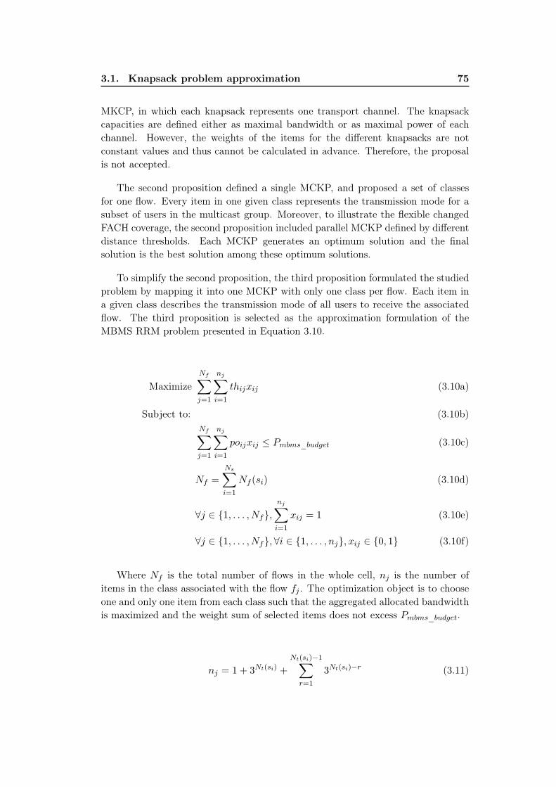
3.1. Knapsack problem approximation 75
MKCP, in which each knapsack represents one transport channel. The knapsackcapacities are defined either as maximal bandwidth or as maximal power of eachchannel. However, the weights of the items for the different knapsacks are notconstant values and thus cannot be calculated in advance. Therefore, the proposalis not accepted.
The second proposition defined a single MCKP, and proposed a set of classesfor one flow. Every item in one given class represents the transmission mode for asubset of users in the multicast group. Moreover, to illustrate the flexible changedFACH coverage, the second proposition included parallel MCKP defined by differentdistance thresholds. Each MCKP generates an optimum solution and the finalsolution is the best solution among these optimum solutions.
To simplify the second proposition, the third proposition formulated the studiedproblem by mapping it into one MCKP with only one class per flow. Each item ina given class describes the transmission mode of all users to receive the associatedflow. The third proposition is selected as the approximation formulation of theMBMS RRM problem presented in Equation 3.10.
MaximizeNf∑j=1
nj∑i=1
thijxij (3.10a)
Subject to: (3.10b)Nf∑j=1
nj∑i=1
poijxij ≤ Pmbms_budget (3.10c)
Nf =
Ns∑i=1
Nf (si) (3.10d)
∀j ∈ 1, . . . , Nf,nj∑i=1
xij = 1 (3.10e)
∀j ∈ 1, . . . , Nf, ∀i ∈ 1, . . . , nj, xij ∈ 0, 1 (3.10f)
Where Nf is the total number of flows in the whole cell, nj is the number ofitems in the class associated with the flow fj . The optimization object is to chooseone and only one item from each class such that the aggregated allocated bandwidthis maximized and the weight sum of selected items does not excess Pmbms_budget.
nj = 1 + 3Nt(si) +
Nt(si)−1∑r=1
3Nt(si)−r (3.11)

76 Chapter 3. Model Analysis
Equation 3.11 computes the number of items nj in the class associated with theflow fj . Let’s assume that fj ∈ F (si). The value 1 represents the item where all usersare served by one FACH. The value 3Nt(si) computes the number of combinationscorresponding to the cases where every user in the multicast group of service si iseither served by DCH, HS-DSCH or not served. When the nearest r users are servedby one FACH, the rest of users have 3Nt(si) − r allocation assignments. Therefore,the number of items in one class is:
nj =
Nt(si)−1∑r=1
3r + 3Nt(si) + 1 =3Nt(si)+1 − 1
2(3.12)
For a given scenario, the total number of items within this scenario is expressedin Equation 3.13. Therefore, the problem complexity is exponential increasing withthe number of users.
Ns∏i=1
Nt(si)∏1
2(3Nf (si) + 1
)(3.13)
The formulation of F2R2M (with channel code constraint relaxed) based onMCKP is achieved. Since MCKP is NP-Hard [74], this proves that the flexibleMBMS RRM problem formulated as F2R2M is also NP-Hard. The complexity ofthe problem increases with the number of MBMS users and services.
3.1.3 Solution bound generation of F2R2M by solving MCKP
To solve the MCKP formulated MBMS RRM problem, different multimediadiffusion scenarios are transferred to MCKP model parameter. These scenarios areshown in Table 3.2.
In this table, each row presents one scenario, the setting of one scenario is in-dicated by its name: the number of service s, the total number of users u and theservice transmission scheme, where S stands for scalable transmission scheme andN stands for non-scalable transmission scheme. The mixed integer programming(MIP) solver Gurobi [46] is used to solve the MCKP by using input parameters.In this work, the MCKP based formulation does not consider the orthogonality ofOVSF code, hence the solutions found by the linear programming solver are thetheoretical solution bounds, but not the real optimum solution of the F2R2M sce-narios. Such solution bound can be used as an indicator to evaluate the real MBMSRRM algorithm performance.

3.1. Knapsack problem approximation 77
Table 3.2: Simulation scenarios for MCKP based formulation
Scenarioname
Flows of service Usernumber
Total trafficrequirement
1s10u128N s1 (f0: 128 kbps) 10 1280 kbps
1s10u128S s1 (f1: 64 kbps, f2: 64 kbps) 10 1280 kbps
2s20uSNs1 (f1: 32 kbps, f2: 32 kbps, f3: 64kbps) 10
2560 kbpss2 (f0: 128 kbps) 10
2s20uSSs1 (f1: 32 kbps, f2: 32 kbps, f3: 64kbps) 10
2560 kbpss2 (f1: 64 kbps, f2: 64 kbps) 10
3s30uSNNs1 (f1: 32 kbps, f2: 32 kbps, f3: 64kbps) 10
3200 kbpss2 (f0: 128 kbps) 10s3 (f0: 64 kbps) 10
3s30uSSNs1 (f1: 32 kbps, f2: 32 kbps, f3: 64kbps) 10
4480 kbpss2 (f1: 64 kbps, f2: 64 kbps) 10s3 (f0: 64 kbps) 10
3.1.3.1 Parameter transformation
In order to solve the MCKP based problem by Gurobi, the scenarios in F2R2Mmust be reformulated into MCKP parameters, which is described in a Gurobi modelfile. Each model file represents all the constraints and the objective described inEquation 3.10a. More precisely, the input model lists the decision variables, thelinear objective function, and finally the linear formulation of constraints. Gurobioptimizer considers all possible values of decision variables that satisfy the givenconstraints, and return the combination of values that optimizes the stated objectivefunction.
To illustrate the nature of the input file of MCKP, an example is given here,which composes one service s0. s0 is scalable transmitted with two flows fs0,1 andfs0,2. The multicast group of s0 includes users t1, t2. According to the MCKP basedformulation, two classes K0,1 and K0,2 are associated with the flows fs0,1 and fs0,2,respectively. Each class includes all potential allocation schemes for the correspond-ing flow. The number of items in each class is 13 (computed by Equation 3.13). Theset of items in each class is shown in Equation 3.14.
Ks0,fj = K0,j = iti,j,k, . . . = it0,j,1, it0,j,2, . . . it0,j,13, j = 1, 2 (3.14)
In Equation 3.14, i is for the service si and the kth item it0,j,k is a candidateallocation scheme for the flow fs0,j . The detailed allocation schemes represented by

78 Chapter 3. Model Analysis
these items are:
K0,1 = K0,2 = tf1 tf2 , t
f1 t
d2, t
f1 t
h2 , t
f1 t
n2 , t
d1t
d2, t
d1t
h2 , t
d1t
n2 , t
h1t
d2, t
h1t
h2 , t
n1 t
d2, t
n1 t
h2 , t
n1 t
n2(3.15)
The item tchm1 tchn
2 represents that the user t1 receives transmission from chm,and the user t2 receives transmission from chn. Each item it0,j,k has two parametersaccording to its allocation scheme: the allocated bandwidth thk and the transmissionpower pok. The solution vector is represented as: x0,1,1 . . . x0,1,13, x0,2,1 . . . x0,2,13,with xi,j,k = 0, 1 and xi,j,k = 1 indicating that the selected allocation scheme isiti,j,k, xi,j,k = 0 means that the corresponding item is not selected in the solution.There is one and only one xi,j,k set to 1, ∀k. With above parameters, the format ofmodel file for Gurobi is shown in Equation 3.16.
MCKP model file:
Maximize Th0,1 + Th0,2 (3.16a)
Subject to
T0,1 : th0,1,1x0,1,1 + th0,1,2x0,1,2 + . . . th0,1,13x0,1,13 − Th0,1 = 0 (3.16b)
P0,1 : po0,1,1x0,1,1 + po0,1,2x0,1,2 + . . . po0,1,13x0,1,13 − Po0,1 = 0 (3.16c)
K0,1 : x0,1,1 + x0,1,2 + . . . x0,1,13 ≤ 1 (3.16d)
T0,2 : th0,2,1x0,2,1 + th0,1,2x0,2,2 + . . . th0,2,13x0,2,13 − Th0,2 = 0 (3.16e)
P0,2 : po0,2,1x0,2,1 + po0,1,2x0,2,2 + . . . po0,2,13x0,2,13 − Po0,2 = 0 (3.16f)
K0,2 : x0,2,1 + x0,2,2 + . . . x0,2,13 ≤ 1 (3.16g)
Pt : Po0,1 + Po0,2 − Ptot = 0 (3.16h)
Pm : Po0,1 + Po0,2 ≤ Pmbms_budget (3.16i)
Binaries
x0,j,k ∈ 0, 1, ∀j, k (3.16j)
Equation 3.16a shows that Gurobi targets at finding the solution to maximizethe allocated throughput of all flows, where Th0,j is the allocated throughput offlow fs0,j . Equation 3.16b to Equation 3.16j illustrate the problem constraints.Equation 3.16b and Equation 3.16e state that Th0,j is the profit (bandwidth) ofthe selected item for the jth class, j = 1, 2. Equation 3.16c and Equation 3.16fstate that Po0,j is the weight of the selected item in the jth class. Constraint K0,j
(Equation 3.16d and Equation 3.16g) guarantees that at least one and only one itemis selected from each class. Constraint Pm (Equation 3.16i)guarantees that the totalweight of the selected items does not exceed the maximum MBMS power budget.Equation 3.16h shows that the total weight Ptot is the sum of Po0,1 and Po0,2. InEquation 3.16j, x0,j,k indicates the selection of the kth item in the jth class.
With the MCKP input model file, Gurobi finds solution with a single objective:the maximum throughput. While in the original F2R2M, the optimization objective

3.2. Fitness landscape analysis 79
has two-dimension (throughput and power). Therefore, the optimization by Gurobionly aims to maximize the allocated throughput (i.e. minimize the throughput loss).To minimize the transmission power, represented by Ptot in Equation 3.16h, the valueof the maximum power budget Pmbms_budget is gradually decreased manually, hencewe obtain different optimum solutions for different Pmbms_budget settings.
3.1.3.2 Gurobi results
The Gurobi model files for small size scenarios are generated and their optimumsolution found by Gurobi are shown in Table 3.3. For large size scenario, for exampleone service with single flow with 17 users, the number of items in each class will be1.937× 109, and the generated model file size is more than 5 Gigabytes. Thereforethe generated MCKP model files for large size scenarios are too large to be handledby the solver.
Table 3.3: Solutions found by Gurobi
Scenarios Gurobi solutions
1s10u128N 0%, 1.352 W
1s10u128S 0%, 1.34 W
2s20uSN 0%, 4.328 W
2s20uSS 0%, 4.263 W
3s30uSNN 0%, 5.297 W
3s30uSSN 0%, 5.231 W
In this work, the MCKP based formulation describes the scenario with relaxedchannel code constraint; the MCKP based formulation does not consider the OVSFcode orthogonality as in F2R2M, thus the channel code are always fully available.Therefore, the solutions solved by MCKP in Table 3.3 are not practical solutionsfor each scenario, but the theoretical solution bounds for MBMS RRM, which couldbe used as the reference for evaluating the practical MBMS RRM algorithms.
3.2 Fitness landscape analysis
Metaheuristic provides efficiency scheme to solve large problem in a reasonabletime consuming. In metaheuristic, the search space is the space of all possiblesolutions that can be visited during the search. In which, a neighborhood operatoris used to move from the current solution to a neighbor solution within the search

80 Chapter 3. Model Analysis
space. By applying one neighborhood operator on the current solution, a set ofneighbor solutions can be generated, constructing the neighborhood of the currentsolution. Therefore, the operator is an essential parameter in metaheuristic as itacts on the dynamics of the search. Different neighborhood can be constructed bydifferent neighborhood operator.
Generally, for a given combinatorial optimization problem, its fitness landscapeis defined as L = (X, f, d) [66, 39], where f denotes the fitness function, X isthe set of solutions depending on the neighborhood structure N and d representsthe distance between two feasible solutions. Therefore, the structure of a fitnesslandscape is linked to the metaheuristic dynamics such as the solutions of the searchspace and the objective functions. Hence the fitness landscape allows to characterizethe problem structure and provides the understanding of the search strategies. It isan important technique to analyze combinatorial optimization problem [75].
In this section fitness landscape analysis technique will be used for analyzing thesolution space of MBMS RRM and evaluating the move operators, which will belater used for metaheuristic searches.
3.2.1 Introduction of fitness landscape analysis
The notion of fitness landscape was firstly proposed in [82], aiming to analyzethe gene interaction in biological evolution. Each genotype has a fitness and thedistribution of the fitness values over the genotypes space constitutes a fitness land-scape.
In chapter 2, two neighborhood operators were proposed to modify the currentsolution to a new solution. They are the single insert operator δSI and the multi-ple insert operator δMI , which define two associated neighborhood structures. Theneighborhood operator is the key element that leads to different optimization per-formance. To characterize the studied problem, the fitness landscape analysis isconducted to analyze the two neighborhood functions for different scenarios. Thisstudy can also help us to determine the better operator in optimization algorithmsby studying the operator performance.
Existing studies [39, 66] have proved that a fitness landscape has several im-portant properties. In our work, we focus on the following properties of a fitnesslandscape:
– the distribution of feasible solutions within the search space.– the distribution of solution fitness.– the links between the solution distance and the difference of solutions fitness.
Generally, to achieve such analysis based on these properties, two sets of solutions

3.2. Fitness landscape analysis 81
are required. Sini is a set of initial solutions randomly chosen from the search space.Slo is a set of local optima solutions found by applying Greedy Local Search (GLS)starting from a solution in Sini. Then the fitness landscape LN is characterizedthrough these two solution sets Sini and Slo.
3.2.2 Solution representations
Two mathematical solution representations are defined, and then the solutiondistance measurement between two feasible solutions are developed. The solutiondistance indicates if the solutions are close to each other. Based on the solutiondistance, then the relationship between the solutions and the landscape can beanalyzed.
3.2.2.1 Representation A
Equation 3.17 shows the solution representation A in which the radio resourceallocation solution of one cell, x(c), is represented as a matrix.
x(c) =
fs1,1 fs1,2 . . . fs1,Nf (s1) . . . fsNs ,Nf (sNs )
ch1,1 ch1,2 . . . ch1,Nf (s1) . . . ch1,Nf
. . . . . . . . . . . . . . . . . .
chi,1 chi,2 . . . . . . . . . chi,Nf
. . . . . . . . . . . . . . . . . .
chNt,1 chNt,2 . . . chNt,Nf (s1) . . . chNt,Nf
(3.17a)
Subject to: (3.17b)
chi,j ∈ −1, 0, 1, 2, 3 (3.17c)
∀i < i′, d(ti) ≤ d(ti′) (3.17d)
x(c) has Nt rows and Nf columns, Nf =∑Ns
i=1Nf (si) in the cell, is the numberof all flows and Nt =
∑Nsi=1Nt(si), is the number of all users in the cell. As shown
in Equation 3.17d, the users are ordered in ascending order of distance from theNode B, therefore, the user ti is closer than the user ti′ , hence i < i′ and di ≤ di′ .An element of this matrix, ch(i, j), indicates the transport channel allocated to theuser ti to receive the flow fj . The value of ch(i, j) could be 0, 1, 2 or 3 if the userti belongs to UEfach(fsi,j), UEdch(fsi,j), UEhs(fsi,j) or UEnoch(fsi,j), respectively.−1 means that the user does not belong to this multicast group.

82 Chapter 3. Model Analysis
3.2.2.2 Representation B
In Equation 3.18, the solution representation B defines that the solution for theflow fs,j is a vector of users.
x(fs,j) = (−1, 1, 2, . . . ,︸ ︷︷ ︸UEfach(fs,j)
−1, i, . . . ,︸ ︷︷ ︸UEdch(fs,j)
−1, j, . . . ,︸ ︷︷ ︸UEhs(fs,j)
−1, k, . . . , tNt︸ ︷︷ ︸UEnoch(fs,j)
) (3.18)
The four user subsets are delimited by the number −1, and indicates the trans-mission channel for the users in each subset. In each subset, users are ordered inascending order of distance from the base station.
Subsequently, the solution of the cell x(c) is a vector of solutions for the servicex(si):
x(c) = x(s1), . . . , x(sNs), ∀si ∈ S(c) (3.19a)
x(si) =
x(fsi,0) if si is a single layer servicex(fsi,1), [x(fsi,2), [x(fsi,3) . . . ]] otherwise
(3.19b)
3.2.3 Distance measurements
The solution distance should evaluate the number of elementary moves requiredto move from one solution to another. In order to conduct the landscape analysis,the distance measurement between the solutions is required.
3.2.3.1 Hamming distance
The hamming distance is a well-known distance in combinatorial optimization,it corresponds to the number of different elements between two solutions. The ham-ming distance dHam is used to measure the distance between two feasible solutionsin the format of the representation A.
3.2.3.2 Comparative distance
For the representation B, the solution distance is measured according to struc-tural comparisons between solutions, named comparative distance dCom. Let’s as-sume that the current solution x and the new solution x′ are based on the represen-tation B. This measurement compares the solutions for the same flow in x and x′,and then the users allocated in the different channel in x and x′ are counted, thisnumber is expressed by dCom.
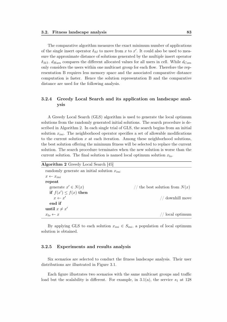
3.2. Fitness landscape analysis 83
The comparative algorithm measures the exact minimum number of applicationsof the single insert operator δSI to move from x to x′. It could also be used to mea-sure the approximate distance of solutions generated by the multiple insert operatorδMI . dHam compares the different allocated values for all users in cell. While dCom
only considers the users within one multicast group for each flow. Therefore the rep-resentation B requires less memory space and the associated comparative distancecomputation is faster. Hence the solution representation B and the comparativedistance are used for the following analysis.
3.2.4 Greedy Local Search and its application on landscape anal-ysis
A Greedy Local Search (GLS) algorithm is used to generate the local optimumsolutions from the randomly generated initial solutions. The search procedure is de-scribed in Algorithm 2. In each single trial of GLS, the search begins from an initialsolution xini. The neighborhood operator specifies a set of allowable modificationsto the current solution x at each iteration. Among these neighborhood solutions,the best solution offering the minimum fitness will be selected to replace the currentsolution. The search procedure terminates when the new solution is worse than thecurrent solution. The final solution is named local optimum solution xlo.
Algorithm 2 Greedy Local Search [45]randomly generate an initial solution xinix← xinirepeat
generate x′ ∈ N(x) // the best solution from N(x)
if f(x′) ≤ f(x) thenx← x′ // downhill move
end ifuntil x 6= x′
xlo ← x // local optimum
By applying GLS to each solution xini ∈ Sini, a population of local optimumsolution is obtained.
3.2.5 Experiments and results analysis
Six scenarios are selected to conduct the fitness landscape analysis. Their userdistributions are illustrated in Figure 3.1.
Each figure illustrates two scenarios with the same multicast groups and trafficload but the scalability is different. For example, in 3.1(a), the service s1 at 128

84 Chapter 3. Model Analysis
−0.5 0 0.5 1 1.50
0.5
1
1.5
2
2 services, 3−sector Node−Bs, site distance = 3000 m
Node B 1
Cell 1
s1: 128 kbps, (32, 32, 64 kbps); 30 ues2: 128 kbps, (64, 64 kbps); 20 ue
(a) scenarios 1,2: 2s50uSN/SS
−0.5 0 0.5 1 1.50
0.5
1
1.5
2
3 services, 3−sector Node−Bs, site distance = 3000 m
Node B 1
Cell 1
s1: 128 kbps, (32, 32, 64 kbps); 30 ues2: 128 kbps, (64, 64 kbps); 20 ues3: 64 kbsp, (64 kbps); 30 ue
(b) scenarios 3,4: 3s80uSNN/SSN
−0.5 0 0.5 1 1.50
0.5
1
1.5
2
3−sector Node−Bs, site distance = 3000 m
Node−B 1
Cell 1
Cell 5
s1: 128 kbps,(32,32,64 kbps);30ues2: 128 kbsp,(64, 64 kbps); 40 ues3: 64 kbsp,(64 kbps); 30 ue
(c) scenarios 5,6: 3s100uSNN/SSN
Figure 3.1: User distributions of six scenarios
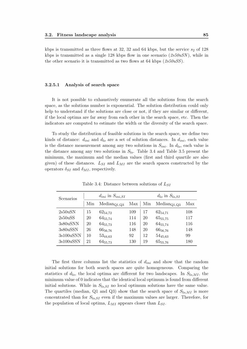
3.2. Fitness landscape analysis 85
kbps is transmitted as three flows at 32, 32 and 64 kbps, but the service s2 of 128kbps is transmitted as a single 128 kbps flow in one scenario (2s50uSN ), while inthe other scenario it is transmitted as two flows at 64 kbps (2s50uSS ).
3.2.5.1 Analysis of search space
It is not possible to exhaustively enumerate all the solutions from the searchspace, as the solutions number is exponential. The solution distribution could onlyhelp to understand if the solutions are close or not, if they are similar or different,if the local optima are far away from each other in the search space, etc. Then theindicators are computed to estimate the width or the diversity of the search space.
To study the distribution of feasible solutions in the search space, we define twokinds of distance: dini and dlo are a set of solution distances. In dini, each valueis the distance measurement among any two solutions in Sini. In dlo, each value isthe distance among any two solutions in Slo. Table 3.4 and Table 3.5 present theminimum, the maximum and the median values (first and third quartile are alsogiven) of these distances. LSI and LMI are the search spaces constructed by theoperators δSI and δMI , respectively.
Table 3.4: Distance between solutions of LSI
Scenariosdini in Sini,SI dlo in Slo,SI
Min MedianQ1,Q3 Max Min MedianQ1,Q3 Max
2s50uSN 15 6254,72 109 17 6254,71 1082s50uSS 20 6455,74 114 20 6555,75 1173s80uSNN 20 6455,73 116 20 6455,74 1163s80uSSN 26 6656,76 148 20 6656,76 1483s100uSNN 10 5344,63 92 12 5445,63 993s100uSSN 21 6455,73 130 19 6555,76 180
The first three columns list the statistics of dini and show that the randominitial solutions for both search spaces are quite homogeneous. Comparing thestatistics of dlo, the local optima are different for two landscapes. In Slo,MI , theminimum value of 0 indicates that the identical local optimum is found from differentinitial solutions. While in Slo,SI no local optimum solutions have the same value.The quartiles (median, Q1 and Q3) show that the search space of Slo,MI is moreconcentrated than for Slo,SI even if the maximum values are larger. Therefore, forthe population of local optima, LMI appears closer than LSI .

86 Chapter 3. Model Analysis
Table 3.5: Distance between solutions of LMI
Scenariosdini in Slo,MI dlo in Slo,MI
Min MedQ1,Q3 Max Min MedQ1,Q3 Max
2s50uSN 19 6253,71 108 0 3423,45 1092s50uSS 23 6454,73 121 0 3322,46 1273s80uSNN 21 6554,73 115 0 4330,57 1383s80uSSN 20 6455,73 116 0 3524,49 1563s100uSNN 24 5564,73 114 0 6339,86 1573s100uSSN 21 6455,73 129 0 3823,56 194
3.2.5.2 Analysis of fitness space
The fitness value represents the quality of a solution. Figure 3.2 shows thedistribution of fitness values of Sini and Slo for 3s100uSNN for both objectives andfor both move operators.
Th(sini) Th(slo)0
10
20
30
40
50
60
70
80
90
100Multiple insert operator
Throughput loss (%)
Po(sini) Po(slo)0
2
4
6
8
10
12
14
16
18
20
Multiple insert operator
Power(W)
Th(sini) Th(slo)0
10
20
30
40
50
60
70
80
90
100Single insert operator
Throughput loss (%)
Po(sini) Po(slo)0
2
4
6
8
10
12
14
16
18
20
Single insert operator
Power(W)
Figure 3.2: Two fitness spaces of scenario 5 (3s100uSNN)
Firstly, it can be observed that the fitness values of Sini are well diversified.According to the similarity of the statistics in Sini for all scenarios (Table 3.4 andTable 3.5), it can be observed that the random initial populations are uniformlydistributed and in a similar way both for δSI and δMI tests. As well, the fitness ofall local optimum for both operators are better than the associated random initial
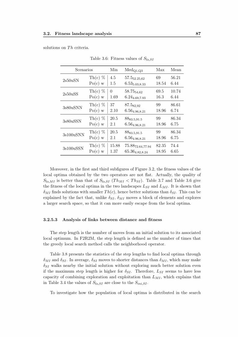
3.2. Fitness landscape analysis 87
solutions on Th criteria.
Table 3.6: Fitness values of Slo,SI
Scenarios Min MedQ1,Q3 Max Mean
2s50uSNTh(c) % 4.5 57.552.25,62 69 56.21Po(c) w 1.5 6.535.03,8.33 18.54 6.44
2s50uSSTh(c) % 0 58.7554,62 69.5 10.74Po(c) w 1.69 6.244.69,7.93 16.3 6.44
3s80uSNNTh(c) % 37 87.582,92 99 86.61Po(c) w 2.10 6.564.96,8.21 18.96 6.74
3s80uSSNTh(c) % 20.5 8883.5,91.5 99 86.34Po(c) w 2.1 6.564.96,8.21 18.96 6.75
3s100uSNNTh(c) % 20.5 8883.5,91.5 99 86.34Po(c) w 2.1 6.564.96,8.21 18.96 6.75
3s100uSSNTh(c) % 15.88 75.8872.64,77.94 82.35 74.4Po(c) w 1.37 65.364.82,8.24 18.95 6.65
Moreover, in the first and third subfigures of Figure 3.2, the fitness values of thelocal optima obtained by the two operators are not flat. Actually, the quality ofSlo,MI is better than that of Slo,SI (ThMI < ThSI). Table 3.7 and Table 3.6 givethe fitness of the local optima in the two landscapes LSI and LMI . It is shown thatδMI finds solutions with smaller Th(c), hence better solutions than δSI . This can beexplained by the fact that, unlike δSI , δMI moves a block of elements and exploresa larger search space, so that it can more easily escape from the local optima.
3.2.5.3 Analysis of links between distance and fitness
The step length is the number of moves from an initial solution to its associatedlocal optimum. In F2R2M, the step length is defined as the number of times thatthe greedy local search method calls the neighborhood operator.
Table 3.8 presents the statistics of the step lengths to find local optima throughδMI and δSI . In average, δSI moves to shorter distances than δMI , which may makeδSI walks nearby the initial solution without exploring much better solution evenif the maximum step length is higher for δSI . Therefore, LSI seems to have lesscapacity of combining exploration and exploitation than LMI , which explains thatin Table 3.4 the values of Slo,SI are close to the Sini,SI .
To investigate how the population of local optima is distributed in the search

88 Chapter 3. Model Analysis
Table 3.7: Fitness values of Slo,MI
Scenarios Min MedQ1,Q3 Max Mean
2s50uSNTh(c) % 0 00,0 58 1.7Po(c) w 7.08 14.8912.95,18.18 19.0 15.28
2s50uSSTh(c) % 0 00,0 62.5 0.94Po(c) w 5.81 14.6314.36,15.02 16.58 14.57
3s80uSNNTh(c) % 0 40,15 91.5 9.43Po(c) w 5.543 17.2915.92,18.79 18.99 17.2
3s80uSSNTh(c) % 0 10,2 93.5 3.8Po(c) w 6.38 17.5717.22,17.63 19.0 17.2
3s100uSNNTh(c) % 0 10,2 93.5 3.8Po(c) w 6.38 17.5717.22,17.63 19.0 17.2
3s100uSSNTh(c) % 1.76 4.124.12,5.88 78.24 7.29Po(c) w 5.67 18.3818.25,18.41 18.99 18.11
space relative to the best solution found, Figure 3.3, Figure 3.4 and Figure 3.5present the plots of fitness distance scatter of all scenarios.
In each subfigure, e.g. Figure 3.3(a), in the left side the y-axis illustrates thefitness difference in terms of throughput loss, and the x-axis illustrates the solutiondistance with dCom. In the right side, the y-axis illustrates the fitness difference interms of power consumption, and the x-axis illustrates the solution distance. Theseplots depict the fitness gap between local optima and best solution found accordingto their distances in terms of required moves number. The plots determine therelationship between the fitness gap and the move distance. When the distance to
Table 3.8: Step lengths of the two landscapes
Scenariostep length in LSI step length in LMI
Min Median Max Mean Min Median Max Mean
2s50uSN 1 7 80 9.70 1 18 57 25.972s50uSS 1 7.5 126 10.74 1 21 62 26.933s80uSNN 1 6 85 8.78 2 43 100 42.693s80uSSN 1 7 127 11.1 1 61 114 67.613s100uSNN 1 7 126 8.94 1 19.5 93 99.883s100uSSN 1 11 181 12.62 5 105 166 99.88

3.2. Fitness landscape analysis 89
0 50 100 150 2000
10
20
30
40
50
60
70
80
90
100
dcom
to best known solution (MI)
∆Th(c)%
0 50 100 150 200−20
−15
−10
−5
0
5
10
15
20
dcom
to best known solution (MI)
∆Po(c)w
0 50 100 150 2000
10
20
30
40
50
60
70
80
90
100
dcom
to best known solution (SI)
∆Th(c)%
0 50 100 150 200−20
−15
−10
−5
0
5
10
15
20
dcom
to best known solution (SI)
∆Po(c)w
(a) scenario 1: 2s50uSN
0 50 100 150 2000
10
20
30
40
50
60
70
80
90
100
dcom
to best known solution (MI)
∆Th(c)%
0 50 100 150 200−20
−15
−10
−5
0
5
10
15
20
dcom
to best known solution (MI)
∆Po(c)w
0 50 100 150 2000
10
20
30
40
50
60
70
80
90
100
dcom
to best known solution (SI)
∆Th(c)%
0 50 100 150 200−20
−15
−10
−5
0
5
10
15
20
dcom
to best known solution (SI)
∆Po(c)w
(b) scenario 2: 2s50uSS
Figure 3.3: Fitness distance scatter: scenarios 1, 2

90 Chapter 3. Model Analysis
the best solution found becomes smaller (the fitness difference is decreased), thesearch procedure is expected to be easier.
Figure 3.3, Figure 3.4 and Figure 3.5 reveal that all local optima converge in asmall region of the search space and the local optima found by δMI are closer tothe best solution found than the local optima found by δSI . When the points arelocated in different distance from the best solution found, their fitness difference arevaried, which means that both search space are rugged. But in the search space ofδSI , the fitness gap and the distance from the best solution found is less correlatedthan in the search space of δMI . The search difficulty with LSI is harder than LMI .
Moreover, the scenarios 1 and 2 (Figure 3.3(a) and Figure 3.3(b)) show highercorrelation than the scenarios 5 and 6, which indicates that the difficulty of exploringthe search space is increased with the increasing of scenario complexity.
Finally, the study of fitness landscape reveals that the local optima in LMI arecloser to each other than in LSI , and that δMI can explore larger neighborhoodspace to reach better solution than δSI . Therefor LMI outperforms LSI .
3.2.5.4 Comparison of two neighborhood operators
Table 3.9 shows the best performance with the two neighborhood operatorsthrough the Greedy Local Search algorithm. The fitness value of the solutions arepresented in terms of the percentage of loss throughput and the consumed power inWatts of all MBMS multicast services within one cell.
Firstly we prove the feasibility of some scenarios with F2R2M. Then δMI alwaysoffers good solution with higher satisfied throughput and less power consumptionthan δSI , which proves that δMI has more ability to escape from local optima, whileδSI can only stay in basins.
3.3 Synthesis
In this chapter, the mathematical analysis was conducted in the proposed flexibleradio resource allocation model for MBMS RRM. In section 3.1, a mathematicalformulation of MBMS RRM is investigated on the basis of the knapsack problemvariants. Three propositions were done to discuss the possibility of this formulation,and the work shows that the single MCKP formulation is the best choice. Thenthe F2R2M is approximated as a MCKP, with the relaxation of the channel codeconstraint. In this formulation, a set of classes are associated with the flows of theMBMS service. Each class includes a set of items, each item is a candidate allocationschemes of the corresponding flow. The problem target is to select one and only one

3.3. Synthesis 91
0 50 100 150 2000
10
20
30
40
50
60
70
80
90
100
dcom
to best known solution (MI)
∆Th(c)%
0 50 100 150 200−20
−15
−10
−5
0
5
10
15
20
dcom
to best known solution (MI)
∆Po(c)w
0 50 100 150 2000
10
20
30
40
50
60
70
80
90
100
dcom
to best known solution (SI)
∆Th(c)%
0 50 100 150 200−20
−15
−10
−5
0
5
10
15
20
dcom
to best known solution (SI)
∆Po(c)w
(a) scenario 3: 3s80uSNN
0 50 100 150 2000
10
20
30
40
50
60
70
80
90
100
dcom
to best known solution (MI)
∆Th(c)%
0 50 100 150 200−20
−15
−10
−5
0
5
10
15
20
dcom
to best known solution (MI)
∆Po(c)w
0 50 100 150 2000
10
20
30
40
50
60
70
80
90
100
dcom
to best known solution (SI)
∆Th(c)%
0 50 100 150 200−20
−15
−10
−5
0
5
10
15
20
dcom
to best known solution (SI)
∆Po(c)w
(b) scenario 4: 3s80uSSN
Figure 3.4: Fitness distance scatter: scenarios 3, 4
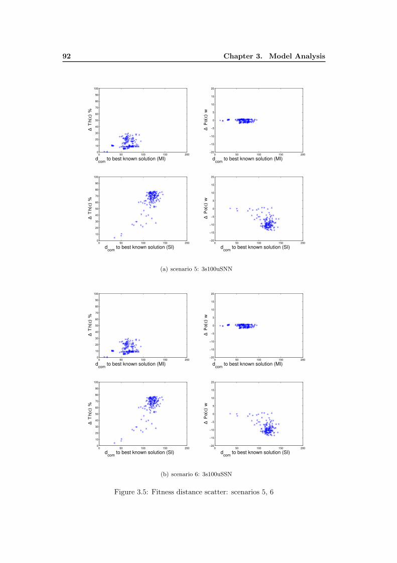
92 Chapter 3. Model Analysis
0 50 100 150 2000
10
20
30
40
50
60
70
80
90
100
dcom
to best known solution (MI)
∆Th(c)%
0 50 100 150 200−20
−15
−10
−5
0
5
10
15
20
dcom
to best known solution (MI)
∆Po(c)w
0 50 100 150 2000
10
20
30
40
50
60
70
80
90
100
dcom
to best known solution (SI)
∆Th(c)%
0 50 100 150 200−20
−15
−10
−5
0
5
10
15
20
dcom
to best known solution (SI)
∆Po(c)w
(a) scenario 5: 3s100uSNN
0 50 100 150 2000
10
20
30
40
50
60
70
80
90
100
dcom
to best known solution (MI)
∆Th(c)%
0 50 100 150 200−20
−15
−10
−5
0
5
10
15
20
dcom
to best known solution (MI)
∆Po(c)w
0 50 100 150 2000
10
20
30
40
50
60
70
80
90
100
dcom
to best known solution (SI)
∆Th(c)%
0 50 100 150 200−20
−15
−10
−5
0
5
10
15
20
dcom
to best known solution (SI)
∆Po(c)w
(b) scenario 6: 3s100uSSN
Figure 3.5: Fitness distance scatter: scenarios 5, 6
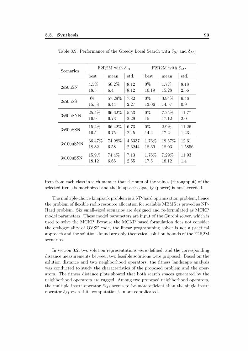
3.3. Synthesis 93
Table 3.9: Performance of the Greedy Local Search with δSI and δMI
ScenariosF2R2M with δSI F2R2M with δMI
best mean std. best mean std.
2s50uSN4.5% 56.2% 8.12 0% 1.7% 8.1818.5 6.4 8.12 10.19 15.28 2.56
2s50uSS0% 57.29% 7.82 0% 0.94% 6.4615.58 6.44 2.27 13.06 14.57 0.9
3s80uSNN25.4% 66.62% 5.53 0% 7.25% 11.7716.9 6.73 2.29 15 17.12 2.0
3s80uSSN15.4% 66.42% 6.73 0% 2.9% 11.2616.5 6.75 2.45 14.4 17.2 1.23
3s100uSNN36.47% 74.98% 4.5337 1.76% 19.57% 12.6118.82 6.58 2.3244 18.39 18.03 1.5856
3s100uSSN15.9% 74.4% 7.13 1.76% 7.29% 11.9318.12 6.65 2.55 17.5 18.12 1.4
item from each class in such manner that the sum of the values (throughput) of theselected items is maximized and the knapsack capacity (power) is not exceeded.
The multiple-choice knapsack problem is a NP-hard optimization problem, hencethe problem of flexible radio resource allocation for scalable MBMS is proved as NP-Hard problem. Six small-sized scenarios are designed and re-formulated as MCKPmodel parameters. These model parameters are input of the Gurobi solver, which isused to solve the MCKP. Because the MCKP based formulation does not considerthe orthogonality of OVSF code, the linear programming solver is not a practicalapproach and the solutions found are only theoretical solution bounds of the F2R2Mscenarios.
In section 3.2, two solution representations were defined, and the correspondingdistance measurements between two feasible solutions were proposed. Based on thesolution distance and two neighborhood operators, the fitness landscape analysiswas conducted to study the characteristics of the proposed problem and the oper-ators. The fitness distance plots showed that both search spaces generated by theneighborhood operators are rugged. Among two proposed neighborhood operators,the multiple insert operator δMI seems to be more efficient than the single insertoperator δSI even if its computation is more complicated.

Chapter 4
Solving MBMS RRM Problem bySimulated Annealing
In chapter 3, the studied MBMS RRM problem has been proved as NP-Hard. Thiscombinatorial optimization problem thus cannot be handled by exhaustive search. Tosolve this problem, the metaheuristic is selected since it requires reasonable amountof effort to get a good (but might be non-optimal) solution. In this chapter, a pop-ular metaheuristic algorithm, the Simulated Annealing (SA) is investigated to solvethe MBMS RRM problem based on F2R2M. This work shows that it is feasible tomodify and map the SA algorithm on the proposed model, named as F2R2M-SA.The simulations are conducted and show that the proposed F2R2M-SA can generatebetter solutions than the state-of-the-art approaches within acceptable time.
Contents4.1 Introduction of simulated annealing algorithm . . . . . . . . 964.2 Algorithm design . . . . . . . . . . . . . . . . . . . . . . . . . . 99
4.2.1 Algorithm framework . . . . . . . . . . . . . . . . . . . . . . 994.2.2 Solution initialization . . . . . . . . . . . . . . . . . . . . . . 1004.2.3 Annealing schedule . . . . . . . . . . . . . . . . . . . . . . . . 1014.2.4 Select_flow(): flow selection . . . . . . . . . . . . . . . . . . . 1014.2.5 Random_move(): solution generation . . . . . . . . . . . . . 1034.2.6 Evaluation(): solution evaluation . . . . . . . . . . . . . . . . 103
4.3 Results and comparison with existing approaches . . . . . . 1054.4 Synthesis . . . . . . . . . . . . . . . . . . . . . . . . . . . . . . 109

96 Chapter 4. Solving MBMS RRM Problem by Simulated Annealing
4.1 Introduction of simulated annealing algorithm
The complexity of the studied problem has been analyzed in chapter 3, and itis proved that the size of the search space increases exponentially with the numberof users. To solve the combinatorial optimization (CO) problem, an algorithm isrequired to find a good (eventually) near-optimal solution, with a reasonable amountof effort. In the past three decades, metaheuristic algorithms tried to combine basicheuristic methods offering efficiency and rapidity [27]. The simulated annealingalgorithm is one of the first metaheuristic that has a strategy to avoid local optima.The origins of this algorithm for solving CO are first presented in [61] and [83].
Simulated annealing is so named because of its similarity to the solid annealingprocess, in which a heated crystalline solid is allowed to cool very slowly until itachieves its minimum lattice energy state, and thus is free of crystal defects [45].The general framework of the simulated annealing is outlined in algorithm 3.
Algorithm 3 General SA algorithm [36]select an initial solution x0select an initial temperature T = T0, T0 ≥ 0
set change counter c = 0
select a repetition schedule, Mk, that defines the number of iterations executedat each temperature, Tk
repeatrepeat
set repetition counter c = 0
generate x′ ∈ N(x)
calculate δ = f(x′)− f(x)
if δ < 0 thenx← x′ // downhill move
else if random(0, 1) < exp(−δTk
) thenx← x′ // uphill move
end ifc← c+ 1
until c = Mk
k ← k + 1
compute Tk
until stopping criterion is met
To describe the features of the general simulated annealing algorithm, severaldefinitions need to be presented. Let Ω be the solution space, let f be an objectivefunction defined on the solution space. The goal is to find an optimum solution x∗,x∗ ∈ Ω such that f(x∗) ≤ f(x), ∀x ∈ Ω. Let’s define N(x) to be the neighborhoodfunction for x ∈ Ω. The neighborhood solution x′ ∈ N(x) can be reached in a single

4.1. Introduction of simulated annealing algorithm 97
iteration by applying a neighborhood operator to the current solution x.
As shown in algorithm 3, SA starts with an initial solution x0 ∈ Ω. The tem-perature parameter T is initialized by a predefined value T0. At each decreasingtemperature Tk, a series of Metropolis chains is performed (the inner loop in algo-rithm 3). The aim of each Metropolis chain is to permit the system to reach thethermal equilibrium, in which the energy state is being minimized. At each iterationwithin the Metropolis chain, a neighborhood solution x′ ∈ N(x) is generated, eitherrandomly or using some pre-specific rules. The candidate solution x′ is accepted asthe current solution x based on the acceptance probability.
The major purpose of the acceptance probability pacc is to accept x′ with theworse result than x, in order to explore new solutions and to escape from localoptimum. pacc is generally computed following the Boltzmann distribution function[45], by Equation 4.1.
pacc =
exp
(−f(x′)−f(x)
Tk
)if f(x′)− f(x) > 0
1 if f(x′)− f(x) ≤ 0(4.1)
where Tk is the temperature parameter at the kth iteration (the outer loop in algo-rithm 3). This acceptance probability is the basic element of the search mechanismin the simulated annealing. f(x′) and f(x) denote the energies (objective functionvalues) associate with the solutions x ∈ Ω and x′ ∈ N(x), respectively. With a fixedtemperature, the higher the difference δ = f(x′) − f(x), the lower the probabilityto accept a move from x to x′. Moreover, the higher is the temperature, the higheris the probability to receive non-improving moves.
In the SA framework, a full annealing schedule is defined by an initial tempera-ture T0, a cooling schedule to reduce the temperature, and a stopping criterion.
The initial temperature should be chosen such that (nearly) every neighborhoodsolution is accepted, thus the entire solution space could be captured. A hightemperature could increase the search space, however it will result in a larger numberof iterations without guarantee on the solution quality. Therefore, T0 is chosen byexperimentation depending upon the problem feature. Van Laarhoven has proposeda method to analytically determine T0 for a given number of solution sampling [48].This procedure starts from a random initial solution with an initial acceptance ratioχ0, and then a series of random walk of solution modifications is performed. In thisrandom walk procedure, for minimization problem, the uphill move, also namedbad move, brings non-improving solution comparing to the current solution. Whilethe downhill move is good move, bringing improvement of the current solution.Equation 4.2 shows the calculation of T0. In Equation 4.2a, ∆f0 is the averageincrease of the objective function between x′ and x during the random walk, andχ0 is the number of accepted bad moves divided by the number of attempted badmoves. In Equation 4.2b, ∆f+ is the increase of fitness between x′ and x, brought
98 Chapter 4. Solving MBMS RRM Problem by Simulated Annealing
by these bad moves.
T0 = −∆f0ln(χ0)
(4.2a)
∆f0 =∆f+
number of accepted bad moves(4.2b)
A similar method of selecting initial temperature, named find-T0 has been pro-posed in [50]. Firstly, T0 is set to zero and a sequence of moves is implemented.After each move, a new value of T0 is calculated according to Equation 4.3.
T0 =∆+
ln( m2m2χ0−m1(1−χ0)
)(4.3a)
∆+ =f(x)− f(x′)
m2(4.3b)
In Equation 4.3a, χ0 is the initial acceptance ratio of bad moves (e.g. set 0.8in [50]). m1 and m2 are the number of good (downhill) and bad (uphill) moves ob-tained so far to solve a minimization problem. For solving a maximization problem,downhill and uphill should be swapped. In Equation 4.3b, x and x′ are respectivelythe current solution and the new solution in each iteration, ∆+ is the average fitnessdifference brought by uphill moves so far. After a given iteration of moves, the finalvalue of T0 is used as the initial temperature.
The cooling schedule determines the decreasing of the temperature in the SAsearch procedure. The earliest annealing schedules were based on the analogy withthe physical annealing. In early SA study, a proportional temperature is used,Tk+1 = αT (k). α is a constant value known as the cooling factor, most of thetime it ranges from 0.80 to 0.99 [76]. At the end of the search, the temperaturedoes not allow any higher energy level, which is called the frozen state. However,[76] concluded that a proportional temperature cooling schedule does not lead toequilibrium at low temperature. Nowadays there are three important annealingschedules to reduce the SA temperature:
– Logarithmic schedule [42], Tk = T0LOG(k) . The temperature decreases quickly at
the beginning of the search, then it decreases slowly. It allows large variationof f for bad solutions at the beginning and small at the end of the search.
– Cauchy schedule [77] is a faster schedule in which Tk = T0k . The Cauchy
schedule allows a regular decreasing of Tk along the search procedure.– Exponential [76] schedule, Tk = Tk−1 exp (−K). It is the fastest schedule andK is a constant value.
Besides, a commonly implemented strategy for reducing the temperature in SAis the linear approach. This strategy reduces the temperature by the same amountthroughout the annealing process: Tk+1 = Tk − t. In which t is a constant whichdescribes the amount of the temperature decrement after each iteration.

4.2. Algorithm design 99
4.2 Algorithm design
To solve the MBMS RRM problem, the general SA algorithm is modified andmapped onto the proposed model, named as F2R2M-SA. We choose SA as it issimple to implement and efficient in term of time cost, it statistically guaranteesfinding a good (enough) solution, and it is adaptable to a variety of problems in-cluding telecommunications [69]. The detailed design of F2R2M-SA algorithm ispresented in this section.
4.2.1 Algorithm framework
Algorithm 4 illustrates the pseudo code of the proposed F2R2M-SA algorithm.The input parameters are the service and user informations collected in the firstphase of model (subsection 2.1.1). The output is the allocation solution for wholecell x(c), which consists the solutions for all flows of all service.
Algorithm 4 F2M2R-SA algorithmRequire: T (c), D(c), S(c), F (si), M(si), ∀si ∈ S(c)
Ensure: x(c) = xfsi,j , ∀si ∈ S(c), ∀j ∈ F (si)x0 ← initialize() // initialize solutionx(c)← x0, x(c)
∗ ← x(c), f∗ ← f(x∗(c))
Tk ← T0 // initialize temperaturewhile Tk > threshold do
for 1 to M dofsi,j ← select_flow(F (si),M(si)) // randomly select one service and flowxf ← extract (x(c), fsi,j) // the flow solution is a part of the cell solutionx′f ← random_move(xf), x′f ∈ N(xf ) // new flow solutioncalculate F (x′f ) = (Th(x′f ), Po(x′f ))
if Po(x′f ) +∑
Po(xfsi,j) > Pmbms_budget,∀fsi,j 6= fsi,j then
reject x′fend ifevaluation(F (xf ), F (x′f )) // evaluation is conducted only on the movedflowif x′f is accepted then
update the cell solution x(c) with x′fend if
end forTk+1 ← cooling(Tk)
end whilereturn x(c)
The algorithm starts by generating an initial solution x(c) for the whole cell. The
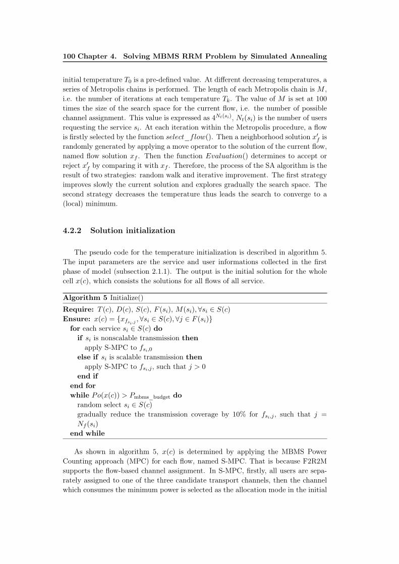
100 Chapter 4. Solving MBMS RRM Problem by Simulated Annealing
initial temperature T0 is a pre-defined value. At different decreasing temperatures, aseries of Metropolis chains is performed. The length of each Metropolis chain is M ,i.e. the number of iterations at each temperature Tk. The value of M is set at 100
times the size of the search space for the current flow, i.e. the number of possiblechannel assignment. This value is expressed as 4Nt(si), Nt(si) is the number of usersrequesting the service si. At each iteration within the Metropolis procedure, a flowis firstly selected by the function select_flow(). Then a neighborhood solution x′f israndomly generated by applying a move operator to the solution of the current flow,named flow solution xf . Then the function Evaluation() determines to accept orreject x′f by comparing it with xf . Therefore, the process of the SA algorithm is theresult of two strategies: random walk and iterative improvement. The first strategyimproves slowly the current solution and explores gradually the search space. Thesecond strategy decreases the temperature thus leads the search to converge to a(local) minimum.
4.2.2 Solution initialization
The pseudo code for the temperature initialization is described in algorithm 5.The input parameters are the service and user informations collected in the firstphase of model (subsection 2.1.1). The output is the initial solution for the wholecell x(c), which consists the solutions for all flows of all service.
Algorithm 5 Initialize()
Require: T (c), D(c), S(c), F (si), M(si), ∀si ∈ S(c)
Ensure: x(c) = xfsi,j , ∀si ∈ S(c), ∀j ∈ F (si)for each service si ∈ S(c) do
if si is nonscalable transmission thenapply S-MPC to fsi,0
else if si is scalable transmission thenapply S-MPC to fsi,j , such that j > 0
end ifend forwhile Po(x(c)) > Pmbms_budget do
random select si ∈ S(c)
gradually reduce the transmission coverage by 10% for fsi,j , such that j =
Nf (si)
end while
As shown in algorithm 5, x(c) is determined by applying the MBMS PowerCounting approach (MPC) for each flow, named S-MPC. That is because F2R2Msupports the flow-based channel assignment. In S-MPC, firstly, all users are sepa-rately assigned to one of the three candidate transport channels, then the channelwhich consumes the minimum power is selected as the allocation mode in the initial
4.2. Algorithm design 101
solution. If the power consuming of the selected (pure) transmission mode is overthe MBMS power budget, a service will be randomly selected, and the farthest usersfor the advanced flow will be gradually rejected until a feasible solution is obtained.
4.2.3 Annealing schedule
As mentioned in section 4.1, a full annealing schedule is defined by the initialtemperature T0, a cooling schedule reducing the temperature, and a stop criteria.
In F2R2M-SA, the method proposed by Van Laarhoven in Equation 4.2 is usedto calculated T0 as in Equation 4.4.
T0 = −∆f0ln(χ0)
= −Po(x′)− Po(x) + Th(x′)− Th(x)
ln(χ0)(4.4)
∆f0 is the average increase in the objective function brought by the uphill moves.
Table 4.1 shows the example of T0 values for 18 scenarios in 10 trials by themethod in Equation 4.4. The number of random walk iterations is 100, and theinitial probability of accepting a bad solution is 0.7 [48]. In each trial, the randomwalk procedure is turned n times, the number of users in each scenario. Thenthe initial temperature for each trial is the rounded integer of the average value:T0 = d 1n
∑ni=1 T
i0e. As shown in Table 4.1, the more the number of users in one
scenario, the larger the value of T0.
For cooling the temperature, we select the logarithmic schedule [42] to decreasethe temperature in F2R2M-SA. In which, the temperature in kth step is determinedby Tk = d T0
LOG(k)e. The stop criterion is when Tk is below a given threshold.
4.2.4 Select_flow(): flow selection
To determine the flow fsi,j to modify, two methods are investigated. The firstmethod randomly selects a flow among all Nf flows in a given scenario, Nf is thetotal number of flows in this scenario. This method randomly selects one servicesi, i ≤ Ns, and then it randomly selects one flow fsi,j from F (si).
The second method determines fsi,j in quasi-determined order. Firstly the ser-vice si is selected in a predefined order (i.e. i is set from 1 to Ns, Ns is the totalnumber of service in one scenario). Then the flow fsi,j is determined:
– j = 0, if si is a non-scalable transmission scheme service.– j = random(1, Nf (si)), if si is a scalable transmission scheme service.
Four scenarios are selected to apply SA with the random flow selection and the

102 Chapter 4. Solving MBMS RRM Problem by Simulated Annealing
Table 4.1: Values of T0 with Equation 4.2
Scenarios T0 in 10 trials Average T0
1s30uN 33 28 29 27 72 13 34 16 29 33 31
1s30uS 51 42 83 31 65 63 28 71 38 63 54
1s60uN 32 98 7 31 47 187 55 17 12 17 51
1s60uS 120 73 104 17 13 132 44 32 122 91 75
1s150uN 344 407 154 86 301 389 196 382 163 155 258
1s150uS 43 106 160 137 299 86 46 191 79 81 123
2s20uSN 22 20 19 12 13 15 5 12 17 16 16
2s20uSS 15 15 7 28 17 18 10 16 23 24 18
2s50uSN 100 53 67 92 75 162 49 45 57 42 75
2s50uSS 112 46 98 48 90 114 35 98 37 138 82
3s30uSNN 88 30 61 37 106 41 37 71 68 64 61
3s30uSSN 27 193 43 20 30 29 46 45 50 85 57
3s50uSNN 35 140 65 74 181 106 55 47 41 45 79
3s50uSSN 98 63 125 32 87 65 75 32 56 61 70
3s80uSNN 55 95 22 54 51 136 106 76 81 163 84
3s80uSSN 114 64 64 58 61 45 78 46 274 79 89
3s100uSNN 167 132 94 85 109 89 71 83 49 50 93
3s100uSSN 75 40 59 36 100 119 65 123 58 92 78

4.2. Algorithm design 103
sequential flow selection methods, respectively. Each algorithm is run 50 trials, thebest solutions found and average solutions are illustrated in Table 4.2. For eachscenario, the best solution is underlined.
Table 4.2: Comparison between two flow selection methods
ScenariosMethod 1: random flow selection Method 2: sequential flow selectionBest solution Average solution Best solutions Average solution
1s60uS 0%, 12.94 W 0%, 13.68 W 0%, 12.82 W 0%, 13.18 W
1s150uS 0%, 15.52 W 0%, 16.07 W 0%, 15.38 W 0%, 15.53 W
2s20uSN 0%, 13.81 W 9.5%, 14.97 W 0%, 7.83 W 0%, 13.18 W
3s50uSSN 5%, 18.87 W 15.19%, 18.26 W 2%, 17.26 W 0%, 18.79 W
Table 4.2 shows that the sequential flow selection method finds better solutionthan the random flow selection method. That is because the sequential flow selectionmethod provides quasi-arbitrary decision instead of full arbitrary decision in thesearch procedure. In the F2R2M-SA implementation, the sequential flow selectionmethod is adopted.
4.2.5 Random_move(): solution generation
In each iteration during the SA procedure, for a given flow fsi,j , a new flowsolution will be randomly selected from the neighborhood of the current flow solutionxfsi,j . Algorithm 6 shows the random generation which randomly moves the currentsolution to generate the new solution x′fsi,j
.
As illustrated in algorithm 6, for the flow solution xfsi,j , according to the UEpartition in xfsi,j , a channel cho will be firstly randomly determined as “output” setand UEcho should not be an empty set. Secondly, a channel chi will be randomlychosen as “input” set, chi 6= cho and chi could be an empty user set. Thirdly, a usertu will be randomly selected from UEcho . Then tu or a set of several users includingtu, constitute the list of users which will be moved from UEcho to UEchi
.
4.2.6 Evaluation(): solution evaluation
Algorithm 7 illustrates the criteria to accept or reject the new flow solution. Thecomparison is conducted between the current flow solution xf (i.e. xfsi,j ), and thenew flow solution x′f (i.e. x′fsi,j
). Each of them should be a part of a feasible cellsolution.

104 Chapter 4. Solving MBMS RRM Problem by Simulated Annealing
Algorithm 6 Random_move()Require: xfsi,jEnsure: generate new flow solution x′fsi,j
service ID = i, flow ID = j
randomly choose cho from xfsi,j , UEcho 6= φ // output (source) channel setrandomly choose chi, (chi 6= cho) // input (target) channel setrandomly choose user tu from UEcho
if cho 6= FACH and chi 6= FACH thenmove tu from cho to chi
elseif cho = FACH then
move user(s) tv and tu from FACH to chi, tv ∈ UEfach, dv ≥ du // theFACH coverage is reduced
else if chi = FACH thenmove user(s) tv and tu from non FACH channels to FACH, tv ∈UEnofach, dv ≤ du // the FACH coverage is increased
end ifend if
Algorithm 7 Evaluation()
Require: x′f , xfEnsure: accept or reject x′f
calculate Th(x′f ), Po(x′f ), Th(xf ), Po(xf )
if Th(x′f ) < Th(xf ) or (Th(x′f ) = Th(xf ) and Po(x′f ) < Po(xf )) thenaccept x′f
elsep← random(0, 1)
if Th(x′f ) > Th(xf ) thenpn = −Kt(Th(x
′f )− Th(xf ))
else if Th(x′f ) = Th(xf ) and Po(x′f ) ≥ Po(xf ) thenpn = −Kp(Po(x′f )− Po(xf ))
end ifpa ← e
pnTk
if p < pa thenaccept x′f // accept x′f with acceptance probability
elsereject x′f
end ifend if

4.3. Results and comparison with existing approaches 105
Based on the proposed lexicographic evaluation criteria in subsection 2.2.4, theevaluator firstly compares the throughput loss because the throughout requirementhas higher priority than the power consumption. Therefore, the solution with lessthroughput loss is the better solution regardless its power consumption. Then forsolutions having the same throughput loss, the solution with less power is better, soif x′f has a better fitness, it is accepted, else it will be accepted with the acceptanceprobability, calculated by Equation 4.5.
pa =
exp(−Kp
Po(x′f )−Po(xf )
Tk
)if Th(x′f ) = Th(xf ) and Po(x′f ) ≥ Po(xf )
exp(−Kt
Th(x′f )−Th(xf )
Tk
)if Th(x′f ) > Th(xf )
(4.5)
The probability factor pa is a function of the current temperature Tk, the fitnessdifference, two factors Kp and Kt. In the proposed model, the two-dimensional fit-ness consists in the bandwidth difference in kilobits per second, and the transmissionpower in Watts; Kt and Kp are defined to calculate pa separately. Kt is set largerthan Kp (Kp = 10,Kt = 50) because the higher constant leads to less acceptanceprobability, then more restriction in the acceptance of the solution with additionalthroughput loss.
4.3 Results and comparison with existing approaches
F2R2M-SA is implemented in the simulator proposed in chapter 2. Togetherwith the competing approaches from the state of the art, they are simulated andcompared under 18 scenarios. The competing approaches are MBMS Power Count-ing (MPC), Dual Transmission mode (Dual Tx), and Scalable FACH transmission(S-FACH). Besides, to prove the advantages of the flow based channel allocation,we apply the MBMS power counting to each flow (S-MPC). To observe the powersaturation, the solutions of MPC, Dual Tx, S-FACH and S-MPC are determined fortheir minimum power consumption, i.e. their solution are accepted no matter if thepower consumption is over the MBMS power budget.
Table 4.3 shows the algorithm solutions for all scenarios. To apply MPC andDual Tx, the services in all the scenarios use non-scalable transmission scheme.Therefore the scenarios have the same service and user distributions share the samesolution, e.g. 1s30uN and 1s30uS. S-FACH allocates the FACH for each flow witha fixed coverage [31]: 95% for f1, or f0 of nonscalable encoded service, 50% for f2and 33% for f3 (if the service has f3).
In Table 4.3, the solutions are presented as two-dimensional fitness value: thelost of throughout in percentage and the consumed power in Watts for all MBMSmulticast services within one cell. For example for scenario 1s30uS, S-FACH applies
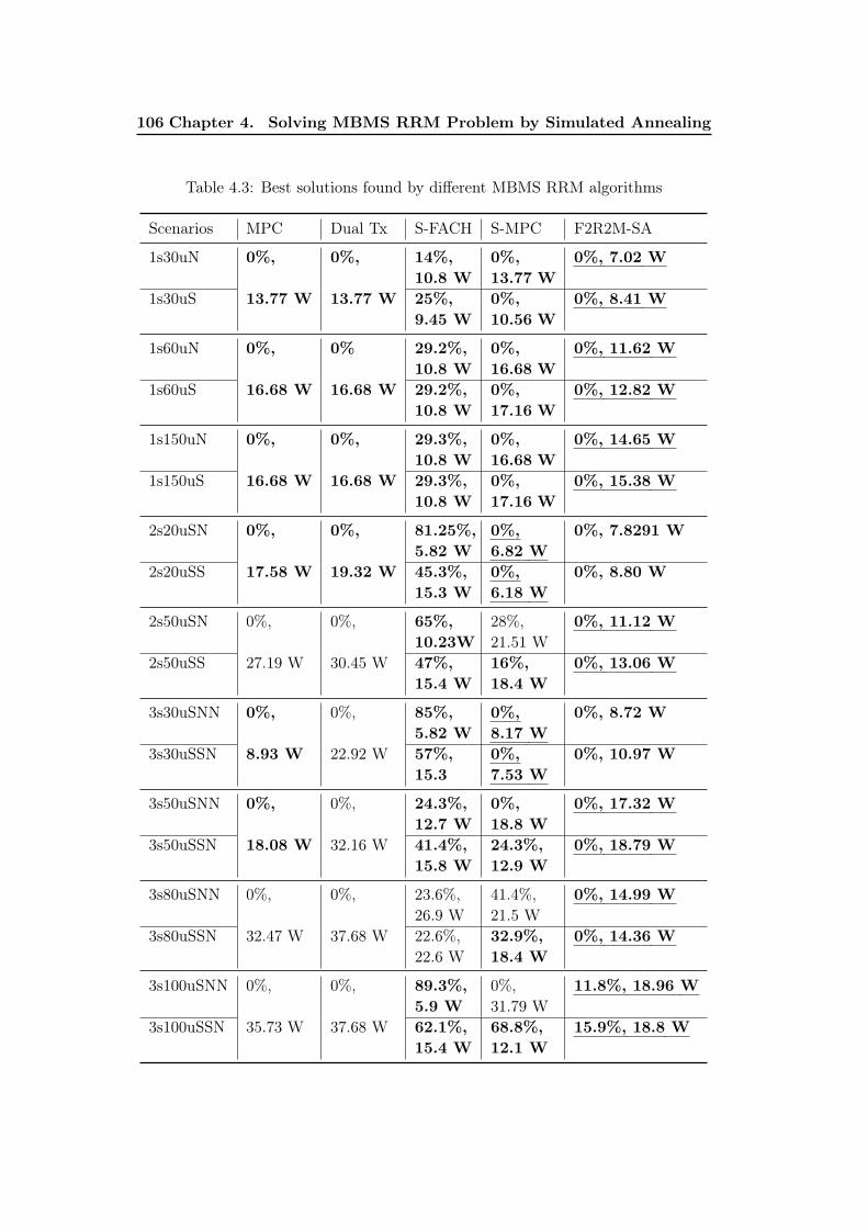
106 Chapter 4. Solving MBMS RRM Problem by Simulated Annealing
Table 4.3: Best solutions found by different MBMS RRM algorithms
Scenarios MPC Dual Tx S-FACH S-MPC F2R2M-SA
1s30uN 0%, 0%, 14%,10.8 W
0%,13.77 W
0%, 7.02 W
1s30uS 13.77 W 13.77 W 25%,9.45 W
0%,10.56 W
0%, 8.41 W
1s60uN 0%, 0% 29.2%,10.8 W
0%,16.68 W
0%, 11.62 W
1s60uS 16.68 W 16.68 W 29.2%,10.8 W
0%,17.16 W
0%, 12.82 W
1s150uN 0%, 0%, 29.3%,10.8 W
0%,16.68 W
0%, 14.65 W
1s150uS 16.68 W 16.68 W 29.3%,10.8 W
0%,17.16 W
0%, 15.38 W
2s20uSN 0%, 0%, 81.25%,5.82 W
0%,6.82 W
0%, 7.8291 W
2s20uSS 17.58 W 19.32 W 45.3%,15.3 W
0%,6.18 W
0%, 8.80 W
2s50uSN 0%, 0%, 65%,10.23W
28%,21.51 W
0%, 11.12 W
2s50uSS 27.19 W 30.45 W 47%,15.4 W
16%,18.4 W
0%, 13.06 W
3s30uSNN 0%, 0%, 85%,5.82 W
0%,8.17 W
0%, 8.72 W
3s30uSSN 8.93 W 22.92 W 57%,15.3
0%,7.53 W
0%, 10.97 W
3s50uSNN 0%, 0%, 24.3%,12.7 W
0%,18.8 W
0%, 17.32 W
3s50uSSN 18.08 W 32.16 W 41.4%,15.8 W
24.3%,12.9 W
0%, 18.79 W
3s80uSNN 0%, 0%, 23.6%,26.9 W
41.4%,21.5 W
0%, 14.99 W
3s80uSSN 32.47 W 37.68 W 22.6%,22.6 W
32.9%,18.4 W
0%, 14.36 W
3s100uSNN 0%, 0%, 89.3%,5.9 W
0%,31.79 W
11.8%, 18.96 W
3s100uSSN 35.73 W 37.68 W 62.1%,15.4 W
68.8%,12.1 W
15.9%, 18.8 W
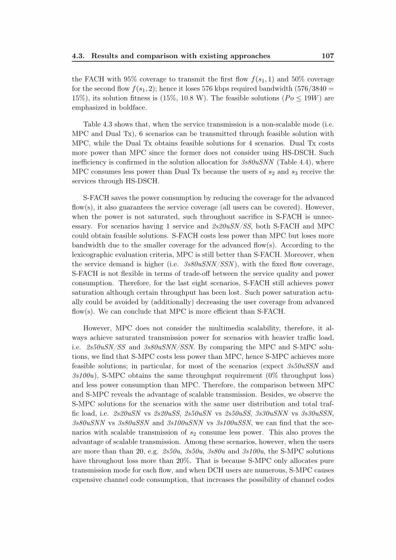
4.3. Results and comparison with existing approaches 107
the FACH with 95% coverage to transmit the first flow f(s1, 1) and 50% coveragefor the second flow f(s1, 2); hence it loses 576 kbps required bandwidth (576/3840 =
15%), its solution fitness is (15%, 10.8 W). The feasible solutions (Po ≤ 19W ) areemphasized in boldface.
Table 4.3 shows that, when the service transmission is a non-scalable mode (i.e.MPC and Dual Tx), 6 scenarios can be transmitted through feasible solution withMPC, while the Dual Tx obtains feasible solutions for 4 scenarios. Dual Tx costsmore power than MPC since the former does not consider using HS-DSCH. Suchinefficiency is confirmed in the solution allocation for 3s80uSNN (Table 4.4), whereMPC consumes less power than Dual Tx because the users of s2 and s3 receive theservices through HS-DSCH.
S-FACH saves the power consumption by reducing the coverage for the advancedflow(s), it also guarantees the service coverage (all users can be covered). However,when the power is not saturated, such throughout sacrifice in S-FACH is unnec-essary. For scenarios having 1 service and 2s20uSN/SS, both S-FACH and MPCcould obtain feasible solutions. S-FACH costs less power than MPC but loses morebandwidth due to the smaller coverage for the advanced flow(s). According to thelexicographic evaluation criteria, MPC is still better than S-FACH. Moreover, whenthe service demand is higher (i.e. 3s80uSNN/SSN ), with the fixed flow coverage,S-FACH is not flexible in terms of trade-off between the service quality and powerconsumption. Therefore, for the last eight scenarios, S-FACH still achieves powersaturation although certain throughput has been lost. Such power saturation actu-ally could be avoided by (additionally) decreasing the user coverage from advancedflow(s). We can conclude that MPC is more efficient than S-FACH.
However, MPC does not consider the multimedia scalability, therefore, it al-ways achieve saturated transmission power for scenarios with heavier traffic load,i.e. 2s50uSN/SS and 3s80uSNN/SSN. By comparing the MPC and S-MPC solu-tions, we find that S-MPC costs less power than MPC, hence S-MPC achieves morefeasible solutions; in particular, for most of the scenarios (expect 3s50uSSN and3s100u), S-MPC obtains the same throughput requirement (0% throughput loss)and less power consumption than MPC. Therefore, the comparison between MPCand S-MPC reveals the advantage of scalable transmission. Besides, we observe theS-MPC solutions for the scenarios with the same user distribution and total traf-fic load, i.e. 2s20uSN vs 2s20uSS, 2s50uSN vs 2s50uSS, 3s30uSNN vs 3s30uSSN,3s80uSNN vs 3s80uSSN and 3s100uSNN vs 3s100uSSN, we can find that the sce-narios with scalable transmission of s2 consume less power. This also proves theadvantage of scalable transmission. Among these scenarios, however, when the usersare more than than 20, e.g. 2s50u, 3s50u, 3s80u and 3s100u, the S-MPC solutionshave throughout loss more than 20%. That is because S-MPC only allocates puretransmission mode for each flow, and when DCH users are numerous, S-MPC causesexpensive channel code consumption, that increases the possibility of channel codes

108 Chapter 4. Solving MBMS RRM Problem by Simulated Annealing
saturation, and leads to high throughput loss.
Table 4.4: Detailed solutions of 3s80uSNN
Algorithms flow Number of users in UE sets
UEfach UEdch UEhs UEnoch
MPC fs1,0 30 0 0 0fs2,0 0 0 20 0fs3,0 0 0 30 0
Dual Tx fs1,0 30 0 0 0fs2,0 20 0 0 0fs3,0 30 0 0 0
Scalable FACH fs1,1 30 0 0 0fs1,2 14 0 0 16fs1,3 5 0 0 25fs2,0 20 0 0 0fs3,0 30 0 0 0
Scalable MPC fs1,1−3 0 0 30 0fs2,0 0 0 20 0fs3,0 0 0 30 0
F2R2M-SA fs1,1−3 0 20 10 0fs2,0 0 10 10 0fs3,0 0 18 12 0
The detailed allocation of different algorithms for 3s80uSNN is illustrated inTable 4.4, which shows that F2R2M-SA avoids the saturation of channel codes byapplying combinational channel assignment of DCH and HS-DSCH for the advancedflow fs1,2−3.
In conclusion, F2R2M-SA outperforms the other algorithms. For small sizescenarios, when the conventional approaches can allocate the radio resources prop-erly, F2R2M-SA consumes less power (47% of MPC solution) by coordinating thethroughput request of the flows and the channel allocation. For large size scenarios,F2R2M-SA avoids the unnecessary throughput loss by more flexibility on the allo-cation of the users to each flow, which allows the algorithm to serve more users forthe advanced flow.

4.4. Synthesis 109
4.4 Synthesis
MBMS RRM problem has been proved to be NP-Hard, which cannot be tackledby exhaustive approach within practical computation time. The selection of meta-heuristic is reasonable, since it requires reasonable amount of effort to get a goodsolution. As a popular and efficient metaheuristic, the Simulated Annealing (SA)has been studied to solve the target problem.
In this chapter, the concept of general SA is firstly introduced. Then a modifiedSA algorithm, named F2R2M-SA is proposed to solve the MBMS RRM problem. Inthe proposed algorithm, the MBMS power counting approach is used to generate theinitial solution. The temperature initialization is applied by a predefined samplingprocedure. For the cooling schedule, the logarithmic cooling schedule is used to de-crease the temperature. At each temperature, the Metropolis chain is implementedwith 100 × 4Nt(si) iterations, Nt(si) is the number of users receiving the flow fsi,j .At each iteration, one application of the neighborhood operator, named the multipleinsert operator, is applied to the current flow solution to randomly generate a newflow solution. When the new solution offers a non-improving fitness (according tothe lexicographic evaluation method), an acceptance probability is calculated by thedifference of solution fitness and two factors Kp and Kt, which are related to thetwo-dimensional fitness value.
Together with the existing MBMS RRM algorithms, the proposed F2R2M-SAis implemented and tested in the same simulation environment. The algorithmperformance is evaluated. Simulation results show that, F2R2M-SA outperforms theother UMTS existing algorithms: MPC, S-FACH and Dual Tx Mode. The proposedmodel provides the best trade off between the power consumption and the servicequality by applying a flow based channel allocation, and reduces the possibility ofradio resource saturation by adapting the combinational channel assignment.


Chapter 5
Solving MBMS RRM Problem byTabu Search
In this chapter, a Tabu Search (TS) algorithm is investigated for solving theMBMS RRM problem. The general TS algorithm is adapted and mapped on theF2R2M, named F2R2M-TS. Comparing with F2R2M-SA which is proposed in chap-ter 4, F2R2M-TS can avoid revisiting previous solutions by keeping memory of previ-ous search steps, which helps to improve the search efficiency. For algorithm design,three tabu memory structures are proposed based on the model characteristics. Theirperformance are compared and evaluated. Furthermore, a tabu repair mechanismis proposed as extension of the classic TS procedure. This mechanism improvesthe search efficiency by self-adapting tabu moves during the search iterations. Theproposed F2R2M-TS is compared with F2R2M-SA and Greedy Local Search (GLS).Simulation results show that F2R2M-TS outperforms the other two algorithms. Thebest solutions found by F2R2M-TS are also compared with the theoretical solutionbounds. Results show that the solutions found by F2R2M-TS are very close or equalto the theoretical optimum solutions.
Contents5.1 Introduction of tabu search algorithm . . . . . . . . . . . . . 1125.2 Algorithm design . . . . . . . . . . . . . . . . . . . . . . . . . . 113
5.2.1 Move operator and neighborhood generation . . . . . . . . . 1155.2.2 Design of tabu memory structures . . . . . . . . . . . . . . . 1175.2.3 Adaptive tabu tenure . . . . . . . . . . . . . . . . . . . . . . 1205.2.4 Tabu repair mechanism . . . . . . . . . . . . . . . . . . . . . 120
5.3 Experiments and results analysis . . . . . . . . . . . . . . . . 1215.3.1 Analysis of tabu search strategies . . . . . . . . . . . . . . . . 1215.3.2 Results comparison with other metaheuristic algorithms . . . 1245.3.3 Performance comparison with theoretical lower bounds . . . . 127
5.4 Synthesis . . . . . . . . . . . . . . . . . . . . . . . . . . . . . . 127

112 Chapter 5. Solving MBMS RRM Problem by Tabu Search
5.1 Introduction of tabu search algorithm
In chapter 3 and chapter 4, the GLS and F2R2M-SA algorithms have been pro-posed to solve the MBMS RRM problem. The simulations show that they havealready outperformed the existing UMTS approaches. However, both of the al-gorithms have the shortcoming that they have difficulties to avoid local optima,making that the best solution found so far is not always found by the algorithms.The Tabu Search (TS) algorithm is studied to overcome this inconvenience.
Tabu search is a metaheuristic search method, originally proposed by Glover in1986 [43]. This algorithm guides a local search procedure to explore the solutionspace beyond local optimality by using memory structures to avoid revisiting previ-ous solutions. In the past decade, several applications of TS have been presented inthe field of wireless networks: frequency and channel assignment [63, 59], node plan-ning and network topology optimization [35], routing optimization [57], etc. Thismakes TS also an attractive candidate for solving MBMS RRM problem. The basicconcept of TS is described in this section.
Tabu search enhances the performance of the classical local search method. Itprevents cycling back to previously visited solutions by using memory structure,called tabu list L. The tabu list records the recent search history, describing therecently visited solutions or pre-defined sets of rules. If a potential solution hasbeen previously visited within a certain period, it is marked as “tabu” (forbidden)so that TS does not consider this solution repeatedly. This memory structure aimsto overcome local optima. Another important element in TS is the neighborhoodstructure. At each iteration, TS starts from the current solution x. The trans-formations that can be applied to x define a set of neighboring solutions, denotedN(x). N(x) is named the neighborhood of x. For any given solution, there aremany possible neighborhood structures defined by different optimization operators.
Algorithm 8 General TS algorithm [44]select an initial solution x0x← x0, f
∗ ← f(x0), x∗ ← x0, L← ∅ // tabu list is empty
repeatselect x′ in argminx′∈N(x)\L[f(x′)] // the best solution among non tabuneighboring solutionsupdate the tabu list L, L← L ∪ xx← x′if f(x) < f∗ thenf∗ ← f(x), x∗ ← x
end ifuntil stopping criterion is met
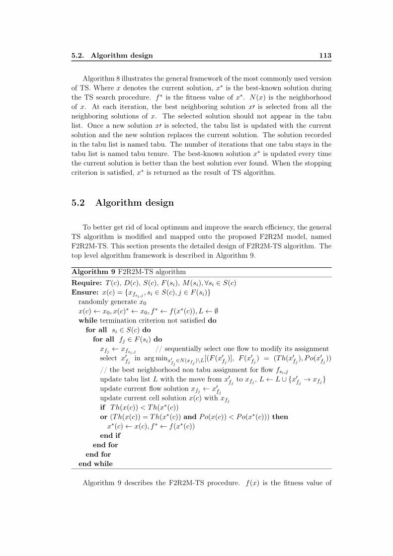
5.2. Algorithm design 113
Algorithm 8 illustrates the general framework of the most commonly used versionof TS. Where x denotes the current solution, x∗ is the best-known solution duringthe TS search procedure. f∗ is the fitness value of x∗. N(x) is the neighborhoodof x. At each iteration, the best neighboring solution x′ is selected from all theneighboring solutions of x. The selected solution should not appear in the tabulist. Once a new solution x′ is selected, the tabu list is updated with the currentsolution and the new solution replaces the current solution. The solution recordedin the tabu list is named tabu. The number of iterations that one tabu stays in thetabu list is named tabu tenure. The best-known solution x∗ is updated every timethe current solution is better than the best solution ever found. When the stoppingcriterion is satisfied, x∗ is returned as the result of TS algorithm.
5.2 Algorithm design
To better get rid of local optimum and improve the search efficiency, the generalTS algorithm is modified and mapped onto the proposed F2R2M model, namedF2R2M-TS. This section presents the detailed design of F2R2M-TS algorithm. Thetop level algorithm framework is described in Algorithm 9.
Algorithm 9 F2R2M-TS algorithmRequire: T (c), D(c), S(c), F (si), M(si), ∀si ∈ S(c)
Ensure: x(c) = xfsi,j , si ∈ S(c), j ∈ F (si)randomly generate x0x(c)← x0, x(c)
∗ ← x0, f∗ ← f(x∗(c)), L← ∅
while termination criterion not satisfied dofor all si ∈ S(c) do
for all fj ∈ F (si) doxfj ← xfsi,j // sequentially select one flow to modify its assignmentselect x′fj in argminx′
fj∈N(xfj
)\L[(F (x′fj )], F (x′fj ) = (Th(x′fj ), Po(x′fj ))
// the best neighborhood non tabu assignment for flow fsi,jupdate tabu list L with the move from x′fj to xfj , L← L ∪ x′fj → xfjupdate current flow solution xfj ← x′fjupdate current cell solution x(c) with xfjif Th(x(c)) < Th(x∗(c))
or (Th(x(c)) = Th(x∗(c)) and Po(x(c)) < Po(x∗(c))) thenx∗(c)← x(c), f∗ ← f(x∗(c))
end ifend for
end forend while
Algorithm 9 describes the F2R2M-TS procedure. f(x) is the fitness value of

114 Chapter 5. Solving MBMS RRM Problem by Tabu Search
the solution x, it includes the throughput loss and the transmission power f(x) =
(Th(x), Po(x)). To optimize the fitness value of the cell solution f(x(c)), F2R2M-TSbegins from an initial solution x0. At each iteration, a given flow fj is sequentiallyselected. The partitioning of UE for the selected flow, xfj , is then explored. Theassociated neighborhood of xfj , named N(xfj ) is generated. Each solution in N(xfj )
could be reached from xfj by an operator named move. The best neighborhoodsolution x′fj is then generated from the feasible and admissible subset of N(xfj ).The tabu list, L, is updated with the reversal move which transfers xfj to x′fj .The tabu list, L, records the active tabu moves (forbidden moves) for a certainnumber of iterations (i.e. tabu tenure). This process is repeated until satisfying thetermination criterion.
In Algorithm 9, a key step is to determine the best flow solution x′fj from theadmissible non tabu neighborhood of the current flow solution N(xfj ), that is togenerate x′fj from N(xfj ). Figure 5.1 illustrates the selection of the best neighboringsolution x′fj in argminx′
fj∈N(xfj
)\L, and the update of the tabu list L.
Select x’fj from N(xfj)
f(x’fj) is the best neighbor found so far?
move(xfj→x’fj) is tabu ?
Still has candidatein N(xfj)?
xfj ← xfj’; x(c) ← x’(c) ; update move(xfj’→xfj) as tabuif f(x(c)) < f(x*(c)) update aspiration criteria
Repaired move(xfj→x’fj)is nonempty?
Tabu repair applied to move(xfj→x’fj )
x’(c) is feasible?
Yes
Add x’fj to N(xfj)
Yes
No
Yes
f(x’(c)) is better than the best-known fitness f(x*(c))?
No
Pass aspiration criteriaYes
Yes
NoNo
Yes
Update x’(c) ← x(c) with x’fj
No
No
Figure 5.1: Best neighborhood selection in F2R2M-TS
As shown in Figure 5.1, at each iteration, for each candidate neighborhood so-lution x′fj , its feasibility and its admissibility is verified. x′fj is called “admissible”

5.2. Algorithm design 115
when it is not classified as tabu or is a tabu move but pass the aspiration criteria.For feasibility control, the new candidate neighborhood solution x′fj will firstly re-place the current flow solution xfj within the current cell solution x(c). Then thepower consumption of the obtained new candidate cell solution, x′(c), is calculated.When Po(x′(c)) is less than the maximum power budget Pmbms_budget, x′(c) (as wellas x′fj ) is called “feasible”. It is necessary that an admissible solution should firstbe a feasible solution.
As shown in Figure 5.1, if x′fj is tabu, the fitness of the solution x′fj will befirstly calculated, and then the fitness of the other flow solutions x′fk , k 6= j, hencethe aggregated fitness value f(x′(c)) is obtained. f(x′(c)) will then be comparedwith the best-known fitness f(x∗(c)). If f(x′c) is better than f(x∗c), x′fj will beaccepted even if it is tabu. This procedure is named aspiration criterion, whichoverrides a solution tabu state when it obtains a fitness value which is better thanthe best ever known flow solution. Then the best known solution and the tabulist will be updated. When x′(c) does not satisfy the aspiration rule, a tabu repairmechanism is proposed to extend the classic tabu search. This mechanism deletesthe tabu attributes from the tabu-declared move that transfers xfj to x′fj , whicheventually leads to a new admissible solution x′fj . x′fj is then be packed in thecandidate solution lists. The aspiration criteria and the repaired tabu mechanismare important elements that introduce flexibility in the solution exploration processof F2R2M-TS.
5.2.1 Move operator and neighborhood generation
In the study of optimization strategies in chapter 3, two move operators aredesigned: the Single Insert (SI) operator δSI (one user moves at a time) and theMultiple Insert (MI) operator δMI (several users move at a time). It is showed thatδMI can easily escape from local optimal solutions while δSI could not escape fromthe initial solution space. Hence it is harder for δSI to get rid of local optimum thanδMI .
Hereby the tabu search neighborhood is considered based on δMI . As introducedin section 2.2, a MI move operation is implemented in five steps:
1. Choose a flow fsi,j to change its current allocation solution xfsi,j .
2. From the UE partition in xfsi,j , choose a channel category iniCh as a “source”set, UEiniCh 6= ∅.
3. From the UE partition in xfsi,j , select a channel category tarCh as a “desina-tion” set, tarCh 6= iniCh.
4. Select one user tk from UEiniCh.

116 Chapter 5. Solving MBMS RRM Problem by Tabu Search
5. According to iniCh and tarCh, move tk or a block of users including tk fromUEiniCh to UEtarCh.
Based on these five steps, the move structure is designed, including five variables,shown in Table 5.1.
Table 5.1: Move structure
Variable Note Value
sId service ID 1, . . . , Ns
fId flow ID 1, . . . , Nf (sId)
iniCh channel ID of source user set 0, 1, 2, 3
tarCh channel ID of destination user set 0, 1, 2, 3
uList list of users to be moved 1, . . . , Nt(sId)
In the move structure, integer values are used to represent the channel ID,hence 0, 1, 2, 3 represent the channels FACH, DCH, HS-DSCH and no transmis-sion (NOCH). uList includes the moved users ID, and depends on the values ofiniCh and tarCh. When the move concerns the source channel is ch1 (DCH) or ch2(HS-DSCH), the δMI operator moves only one user. While for the source channelch0 (FACH), the moved users depends on the changed FACH coverage. For exam-ple, if the user tk is moved from UEhs to UEfach, the FACH coverage is extended toreach tk and all the users nearer than tk can now hear from FACH transmission andshould be (if currently they are not in) moved to FACH user set. Therefore, when tkis chosen to be inserted into UEfach, F2R2M-TS will first check the distribution ofusers served by the other channels, and then pick out the users within the enlargedcoverage to UEfach. At the contrary, if the source channel iniCh is FACH, themove will leads to reducing the FACH coverage and all users farther than tk withinUEfach should be inserted to UEtarCh.
x1 : (−1 1 2 3 4 5︸ ︷︷ ︸ −1 7 8︸ ︷︷ ︸ −1 6 9 10︸ ︷︷ ︸ −1 11︸ ︷︷ ︸) (5.1a)
x2 : (−1 1︸ ︷︷ ︸ −1 7 8︸ ︷︷ ︸ −1 2 3 4 5 6 9 10︸ ︷︷ ︸ −1 11︸ ︷︷ ︸) (5.1b)
x3 : (−1 1︸ ︷︷ ︸ −1 2 7 8︸ ︷︷ ︸ −1 3 4 5 6 9 10︸ ︷︷ ︸ −1 11︸ ︷︷ ︸) (5.1c)
x4 : (−1 1︸ ︷︷ ︸ −1 2 3 7 8︸ ︷︷ ︸ −1 4 5 6 9 10︸ ︷︷ ︸ −1 11︸ ︷︷ ︸) (5.1d)
x5 : (−1 1︸ ︷︷ ︸ −1 2 3 4 7 8︸ ︷︷ ︸ −1 5 6 9 10︸ ︷︷ ︸ −1 11︸ ︷︷ ︸) (5.1e)
In Equation 5.1, five examples of δMI operators are conducted. This example

5.2. Algorithm design 117
shows a case where the cell includes only one service with one flow and the solution ischanged from x1 to x2 and so on until x5. According to the solution representationintroduced in chapter 3, solutions are represented as a vector of four user sets:UEfach, UEdch, UEhs and UEnoch, these user subsets are delimited by −1. In eachsubset, users are ordered in ascending order of their distances from the base station.
Table 5.2 describes the first move, m1, modifying the solution x1 to x2.
Table 5.2: A move example m1: from x1 to x2
Variable sId fId iniCh tarCh uList
Value 1 1 0 2 2, 3, 4, 5
The users t2, t3, t4 and t5 are moved from the FACH channel to a HS-DSCHchannel with tk = t2. The coverage threshold dthr is set to d2. t1 is kept withinthe FACH coverage because it is the nearest user from the base station. Whereas ifdthr < d1, the FACH coverage would be further reduced, bringing out the t1 fromthe FACH coverage. Then from x3 to x5, one user is selected to move from theHS-DSCH to the DCH channel.
Algorithm 10 shows the neighborhood generation of solution xfsi,j , based onδMI .
5.2.2 Design of tabu memory structures
The tabu list is a memory structure dynamically modified during the searchprocedure. The tabu search records the characteristics of previous moves. Once asolution is updated, the modified attributes by the current move will be set tabuactive, and recorded in the tabu list. In the following iterations, the tabu evaluationprocedure compares the attributes of a potential move operation with the tabuattributes stored in the tabu list. The move is considered as tabu if a matching isfound. The moves declared as tabu will be ignored except if it satisfies the aspirationcriterion. By doing this, re-visiting of recent solutions through non-improving movesare prevented. In TS heuristic, tabu memory structures plays an important role inthe algorithm performances. Based on the move operator, three tabu structures aredefined. As shown in Table 5.3, these move based tabu structures include three,four and five variables, respectively.
As shown in Table 5.3, the reverse move of the selected one is considered astabu. In addition to definitions in Table 5.1, uId refers to the user that recentlymoved in a recent iteration. tabu-tri means that the current transmission channelof the user uId on the flow fId belonging to the service sId is tabu-active (shouldtemporarily not be modified). tarCh represents the target channel for uId, therefore

118 Chapter 5. Solving MBMS RRM Problem by Tabu Search
Algorithm 10 Neighborhood_generate()Require: xfsi,j
,M(si), i ∈ S(c), j ∈ Nf (si)
Ensure: N(xfsi,j)
for all user t ∈M(si) doUEnofach = ∪ch 6=fachUEch(fsi,j)
if t ∈ UEfach(fsi,j) thenfor all tar = 1 or 2 or 3 do
new move: sId = i; fId = j; iniCh = 0; tarCh = tar
uList = v ∈ UEfach(fsi,j), dv < dtend for
end ifif t ∈ UEdch(fsi,j) then
for all tar = 0 or 2 or 3 donew move: sId = i; fId = j; iniCh = 1; tarCh = tar
if tar = 0 thenuList = v ∈ UEnofach, dv ≤ dt
elseuList = t
end ifend for
end ifif t ∈ UEhs(fsi,j) then
for all tar = 0 or 1 or 3 donew move: sId = i; fId = j; iniCh = 2; tarCh = tar
if tar = 0 thenuList = v ∈ UEnofach, dv ≤ dt
elseuList = t
end ifend for
end ifif t ∈ UEnoch(fsi,j) then
for all tar = 0 or 1 or 2 donew move: sId = i; fId = j; iniCh = 3; tarCh = tar
if tar = 0 thenuList = v ∈ UEnoch(fsi,j), dv ≤ dt
elseuList = t
end ifend for
end ifend for

5.2. Algorithm design 119
Table 5.3: Three tabu structure definitions
tabu-tri tabu-qua tabu-pen
sId sId sId
fId fId fId
uId uId uId
tarCh tarCh
iniCh
tabu-qua stipulates that a given destination channel for uId is tabu-active, whichmeans that the reallocation of a given type of channel to the user is not allowed forthis flow. Finally, tabu-pen sets that the transfer of user uId from iniCh to tarChis tabu-active. tabu-tri is the most restrictive tabu structure.
Following the example in Equation 5.1, m1 transfers x1 to x2. Because x2 is thebest neighbor, it replaces x1, and the reverse move of m1 is recorded as tabu, asshown in Table 5.4. The tarCh and iniCh in tabu elements are, respectively, theinitial channel and the target channel in the move operator.
Table 5.4: Tabus states (type tabu-pen) based on move m1
Variables tabu1 tabu2 tabu3 tabu 4
sId 1 1 1 1
fId 1 1 1 1
uId 2 3 4 5
iniCh 2 2 2 2
tarCh 0 0 0 0
5.2.2.1 Tabu evaluation
During the search iterations, the potential moves are evaluated by comparing themove attributes with the tabu elements stored in the tabu list. A move is declaredas tabu when a matching is found. Only one type of tabu structure is applied ineach TS procedure. Assume that tabu-pen is decided to evaluate the tabu moves, amove for x5 cannot put the users t2 or t3 from the iniCh 2 to the tarCh 0 as thosemoves are tabu.

120 Chapter 5. Solving MBMS RRM Problem by Tabu Search
Table 5.5: A tabu move for x5
Variable sId fId iniCh tarCh uList
Value 1 1 2 (HS-DSCH) 0 (FACH) 2, 3
5.2.3 Adaptive tabu tenure
The number of iterations that an attribute remains tabu-active is called its tabutenure. In general it could be fixed as predefined value or dynamically calculated.Several studies [34, 71] have shown that a dynamic tabu tenure could be moreeffective than a static value. Here, the tabu tenure varies for different tabu attributesand different problem sizes, which provides a dynamic and robust form of search[44]. In this work, the dynamic tabu tenure is randomly selected from the interval[√N2 , 3
√N2 ], where the value of N depends on the type of tabu attribute. Assume that
an instance has Ns services, each has Nf (si) = Nf flows and Nt(si) = Nt users. Inthe case of tabu-pen structure there are N = 12 ·Ns ·Nf ·Nt possible moves (channelmodification) from a current solution. Similarly, for tabu-qua, N is the number ofpossible target channel setting for the whole problem, hence N = 3 · Ns · Nf · Nt.Finally, for tabu-tri, N = Ns · Nf · Nt. Therefore, the more restrictive the tabustructure is, the shorter the tabu tenure, and consequentially the shorter the tabulist.
5.2.4 Tabu repair mechanism
To explore new candidate solutions, the tabu repair mechanism is proposed basedon the definitions of tabu and the move structure. It is done by re-allowing a tabu-declared move by modifying a sub-set of its attributes. In this application, the userattribute is modified by the tabu repair mechanism.
1sId
1fId
2iniCh
0tarCh
5 6 9 10uList
Tabu elements, to delete from uList
1sId
1fId
2iniCh
0tarCh
6 9 10uList
Tabu Move
Repaired Move
Figure 5.2: Tabu repair mechanism: an example
As illustrated in Figure 5.2, a tabu move is selected to be applied to x5: movethe users t5, t6, t9 and t10 from HS-DSCH to FACH. The selected move is tabu
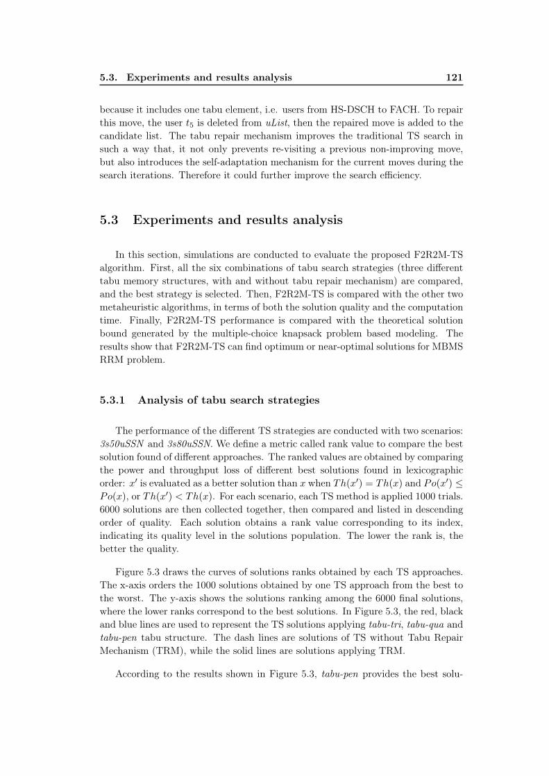
5.3. Experiments and results analysis 121
because it includes one tabu element, i.e. users from HS-DSCH to FACH. To repairthis move, the user t5 is deleted from uList, then the repaired move is added to thecandidate list. The tabu repair mechanism improves the traditional TS search insuch a way that, it not only prevents re-visiting a previous non-improving move,but also introduces the self-adaptation mechanism for the current moves during thesearch iterations. Therefore it could further improve the search efficiency.
5.3 Experiments and results analysis
In this section, simulations are conducted to evaluate the proposed F2R2M-TSalgorithm. First, all the six combinations of tabu search strategies (three differenttabu memory structures, with and without tabu repair mechanism) are compared,and the best strategy is selected. Then, F2R2M-TS is compared with the other twometaheuristic algorithms, in terms of both the solution quality and the computationtime. Finally, F2R2M-TS performance is compared with the theoretical solutionbound generated by the multiple-choice knapsack problem based modeling. Theresults show that F2R2M-TS can find optimum or near-optimal solutions for MBMSRRM problem.
5.3.1 Analysis of tabu search strategies
The performance of the different TS strategies are conducted with two scenarios:3s50uSSN and 3s80uSSN. We define a metric called rank value to compare the bestsolution found of different approaches. The ranked values are obtained by comparingthe power and throughput loss of different best solutions found in lexicographicorder: x′ is evaluated as a better solution than x when Th(x′) = Th(x) and Po(x′) ≤Po(x), or Th(x′) < Th(x). For each scenario, each TS method is applied 1000 trials.6000 solutions are then collected together, then compared and listed in descendingorder of quality. Each solution obtains a rank value corresponding to its index,indicating its quality level in the solutions population. The lower the rank is, thebetter the quality.
Figure 5.3 draws the curves of solutions ranks obtained by each TS approaches.The x-axis orders the 1000 solutions obtained by one TS approach from the best tothe worst. The y-axis shows the solutions ranking among the 6000 final solutions,where the lower ranks correspond to the best solutions. In Figure 5.3, the red, blackand blue lines are used to represent the TS solutions applying tabu-tri, tabu-qua andtabu-pen tabu structure. The dash lines are solutions of TS without Tabu RepairMechanism (TRM), while the solid lines are solutions applying TRM.
According to the results shown in Figure 5.3, tabu-pen provides the best solu-

122 Chapter 5. Solving MBMS RRM Problem by Tabu Search
0 200 400 600 800 10000
1000
2000
3000
4000
5000
6000
Solution indexed in descending order of quality
Sol
utio
n R
ank
3s50uSSN
tri w reptri wo repqua w repqua wo reppen w reppen wo rep
(a) 3s50uSSN
0 200 400 600 800 10000
1000
2000
3000
4000
5000
6000
Solution indexed in descending order of quality
Sol
utio
n R
ank
(the
low
er th
e be
tter)
3s80uSSN
tri w reptri wo repqua w repqua wo reppen w reppen wo rep
(b) 3s80uSSN
Figure 5.3: TS strategies comparison

5.3. Experiments and results analysis 123
tions set among the three tabu structures and tabu-qua provides the worse solutionsquality. The comparison of the six TS strategies according to the tabu repair mech-anism shows that this mechanism significantly improves the solution whatever thetabu structure.
Table 5.6 and Table 5.7 illustrate the best solutions found (among 150 trials)of tabu search with and without tabu repair mechanism. The solution fitness arerepresented in two dimensions: Th(x) in percentage and Po(x) in Watts. Themaximum power budget is set to 19 W (solutions with Th(x) < 19 are feasible)and all solutions are feasible. The solutions found by TRM approach (Table 5.6)consume less power than without TRM in Table 5.7, which confirms the conclusionsof Figure 5.3(a) and Figure 5.3(b).
Table 5.6: TS solutions without tabu repair mechanism
Scenarios tabu-tri tabu-qua tabu-pen
1s60uS 0%, 12.46 W
1s150uS 0%, 15.38 W
2s50uSN 0%, 11.16 W 0%, 11.27 W 0%, 11.12 W
2s50uSS 0%, 10.71 W 0%, 10.74 W 0%, 10.70 W
3s50uSNN 0%, 9.27 W 0%, 9.50 W 0%, 9.27 W
3s50uSSN 0%, 9.27 W 0%, 9.53 W 0%, 9.27 W
3s80uSNN 0%, 14.07 W 0%, 14.46 W 0%, 14.06 W
3s80uSSN 0%, 13.45 W 0%, 13.59 W 0%, 13.50 W
Table 5.7: TS solutions with tabu repair mechanism
Scenarios tabu-tri tabu-qua tabu-pen
1s60uS 0%, 12.46 W
1s150uS 0%, 15.38 W
2s50uSN 0%, 11.12 W 0%, 11.17 W 0%, 11.12 W
2s50uSS 0%, 10.70 W 0%, 10.73 W 0%, 10.54 W
3s50uSNN 0%, 9.27 W 0%, 9.5 W 0%, 9.27 W
3s50uSSN 0%, 9.27 W 0%, 9.40 W 0%, 9.27 W3s80uSNN 0%, 14.07 W 0%, 14.26 W 0%, 14.06 W
3s80uSSN 0%, 13.43 W 0%, 13.50 W 0%, 13.43 W
Table 5.7 indicates that TS with tabu-pen always provides the best solution

124 Chapter 5. Solving MBMS RRM Problem by Tabu Search
(underlined). This tabu declaration method is less strict than the two others, henceit provides more flexible neighborhood exploration. Moreover, although tabu-tri isthe most strict tabu type, the adaptive tabu tenure mechanism loosens its stringency.The tabu list for tabu-tri is shorter since it has smaller tenure. Therefore, it cansometimes also find good solutions as tabu-pen. Besides, the solutions in Table 5.7are better than those of Table 5.6, which shows the advantage of the tabu repairmechanism.
5.3.2 Results comparison with other metaheuristic algorithms
The proposed TS algorithm is compared with the Greedy Local Search (GLS)in chapter 3 and the Simulated Annealing (SA) in chapter 4. In Figure 5.4, thebars show the rank distributions of F2R2M-TS, GLS and F2R2M-SA solutions forfour scenarios. Here F2R2M-TS applies the tabu repair mechanism and uses thetabu-pen structure to record the tabu moves.
−200 0 200 400 600 800 10000
20
40
60
80
100
RankingOrder
RankingDistribution
3s50uSNN
F2R2M-TS
GLS
F2R2M-SA
−200 0 200 400 600 800 10000
20
40
60
80
100
RankingOrder
RankingDistribution
3s50uSSN
F2R2M-TS
GLS
F2R2M-SA
−200 0 200 400 600 800 10000
20
40
60
80
100
RankingOrder
RankingDistribution
3s80uSNN
F2R2M-TS
GLS
F2R2M-SA
−200 0 200 400 600 800 10000
20
40
60
80
100
RankingOrder
RankingDistribution
3s80uSSN
F2R2M-TS
GLS
F2R2M-SA
Figure 5.4: Rank distributions of three metaheuristic algorithms
GLS starts from a random initial solution, evaluates all its feasible neighbors andreplaces the current solution by the neighborhood solution that has the best fitness.GLS stops at the local optimum when no neighbor is better than the current solution.F2R2M-SA generates an initial solution by scalable MBMS power counting, then
5.3. Experiments and results analysis 125
it randomly modifies the current solution in each iteration. The new solution willbe accepted if it has better fitness than the current one, else it is accepted withan acceptance probability depending on the current temperature. 100 × 4Nt(si)
iterations are performed at each temperature until the temperature declines under agiven threshold. The following experiments are conducted to perform the algorithmcomparison. For each given scenario, each algorithm is run 300 times. All solutionsof these algorithms are ordered in the same database. The ranking number rangesfrom 1 to 900 and the smaller the rank is, the better the solution. This range isdivided into 16 subsets, the number of ranking values in each subset is then counted.Such number reflects the ranking distribution and shows the distribution of solutionranking for a corresponding algorithm.
Table 5.8 lists the best solutions found by the three metaheuristics over the18 scenarios (each algorithm runs 300 trials per scenario). The feasible solutions(Po < 19W ) are underlined.
In Table 5.8, for the small-sized scenarios (one service), all algorithms can findthe same solutions, for both scalable and non-scalable transmission schemes. Thatis because the landscape of these scenarios is quite smooth, having few local optima.
However, for the large-sized scenarios, F2R2M-TS outperforms GLS while F2R2M-SA obtains worse solution than GLS. GLS is the most simple heuristic, but is notrobust in terms of solution quality. A well-known disadvantage of GLS is that, whenit reaches a state where no further improvement can be found, GLS stops the so-lution modification and output the current solution, such states are referred to aslocal optimum.
Besides, although SA is easy to implement and adaptable [69], the randomnessof the solution update mechanism and the complex search parameter setting (i.e.cooling schedule and acceptance possibility) bring instability in solution quality.Because the solution spaces of the large-sized scenarios are rugged, SA is not suit-able for F2R2M for its randomness characteristics in new solution selection andacceptance. It should need more tests with different parameter setting to improveit.
In this work, the simulations are conducted on Linux PC with Intel(R) Core(TM)i5 CPU 750 @ 2.67GHz. Table 5.9 shows the average computation time of the threeapproaches for all scenarios on 300 runs. The consuming time of the search procedurein F2R2M-TS is about 1 to 3 seconds in the regular Linux PC. It is acceptable fora RNC server. A stop criterion is defined both in F2R2M-SA and F2R2M-TS;they stop when the consecutive number of iterations with non-improving solutions(comparing to the best solution found) is more than 100Nf , where Nf is the totalnumber of flows in the cell. GLS costs the shortest time since it does not conduct thetabu evaluation. For simple scenarios, F2R2M-TS costs longer time than F2R2M-SA because it requires to evaluate and update the tabu list. For complex scenarios,

126 Chapter 5. Solving MBMS RRM Problem by Tabu Search
Table 5.8: Best solutions found by three metaheuristic algorithms
Scenarios F2R2M-TS GLS F2R2M-SA
1s30uN 0%, 5.18 W 0%, 5.18 W 0%, 5.18 W
1s30uS 0%, 5.31 W 0%, 5.31 W 0%, 5.31 W
1s60uN 0%, 11.62 W 0%, 11.62 W 0%, 11.62 W
1s60uS 0%, 12.82 W 0%, 12.82 W 0%, 12.82 W
1s150uN 0%, 14.65 W 0%, 14.65 W 0%, 14.65 W
1s150uS 0%, 15.38 W 0%, 15.38 W 0%, 15.38 W
2s20uSN 0%, 4.328 W 0%, 4.66 W 0%, 7.83 W
2s20uSS 0%, 4.35 W 0%, 5.12 W 0%, 8.80 W
2s50uSN 0%, 11.12 W 0%, 11.17 W 0%, 10.19 W
2s50uSS 0%, 10.94 W 0%, 10.92 W 0%, 13.06 W
3s30uSNN 0%, 5.33 W 0%, 6.15 W 0%, 8.72 W
3s30uSSN 0%, 5.31 W 0%, 6.27 W 0%, 10.97 W
3s50uSNN 0%, 9.27 W 0%, 11.18 W 0%, 18.8 W
3s50uSSN 0%, 9.27 W 0%, 11.38 W 0%, 18.79 W
3s80uSNN 0%, 14.06 W 0%, 14.49 W 0 %, 15 W
3s80uSSN 0%, 13.43 W 0%, 14.52 W 0%, 14.36 W
3s100uSNN 2.35 %, 18.11 W 4.12 %, 17.51 W 11.77 %, 18.96 W
3s100uSSN 0.59 %, 17.86 W 1.76 %, 18.11 W 15.89 %, 18.79 W
Table 5.9: Average time cost (second)
Scenario F2R2M-TS GLS F2R2M-SA
1s60uS 0.65 0.02 0.81
1s150uS 1.01 0.04 0.92
2s50uSN 1.36 0.16 1.24
2s50uSS 1.42 0.26 1.35
3s50uSNN 1.87 0.32 1.82
3s50uSSN 1.84 0.28 1.95
3s80uSNN 2.88 0.37 3.52
3s80uSSN 2.99 0.34 3.78

5.4. Synthesis 127
F2R2M-SA costs much longer time than F2R2M-TS because at each iteration theprobability of randomly generating an unfeasible solutions is too high, therefore,the most computation time is spent on searching for (randomly pick out) a feasiblesolution. As F2R2M-TS can quickly find a good enough solution, the non-improvingiteration number larger than 100Nf is earlier satisfied than for F2R2M-SA for thecomplex scenarios.
5.3.3 Performance comparison with theoretical lower bounds
In chapter 3, it has been shown that MBMS RRM problem can be approximatedas a Multiple-Choice Knapsack Problem (MCKP) when relaxing the OVSF codeconstraints. Solving the MCKP gives the solution lower bound for the MBMSRRM problem, which can be considered as the approximation of the MBMS RRMoptimum solution. In this section, to better evaluate the performance of F2R2M-TS,a comparison is conducted between F2R2M-TS and the theoretical solution bound.Table 5.10 shows the lower bounds by solving the MCKP using Gurobi solver, andthe best solutions found by using F2R2M-TS. It shows that, in the given scenarios,F2R2M-TS can find the optimum or near-optimum solutions.
Table 5.10: Solution lower bounds found by Gurobi and the best solutions found byF2R2M-TS
Scenarios Gurobi F2R2M-TS
1s10u128N 0%, 1.352 W 0%, 1.352 W
1s10u128S 0%, 1.34 W 0%, 1.34 W
2s20uSN 0%, 4.328 W 0%, 4.328 W
2s20uSS 0%, 4.263 W 0%, 4.346 W
3s30uSNN 0%, 5.297 W 0%, 5.328 W
3s30uSSN 0%, 5.231 W 0%, 5.314 W
5.4 Synthesis
In this chapter, the Tabu Search (TS) algorithm is conceived to solve the MBMSRRM problem. First, the general concepts of TS are introduced then an adaptationof TS algorithm, named F2R2M-TS, is proposed to solve the MBMS RRM problem.
In the proposed algorithm the move structure is designed based on the multipleinsert operator δMI . Each move includes five parameters. From the move structure,

128 Chapter 5. Solving MBMS RRM Problem by Tabu Search
the neighborhood generation is illustrated. This procedure explores all the candidatemoves and constructs the candidate move list.
The tabu memory structure plays a key role for the search efficiency. Threetabu structures are proposed for tabu declaration. Tabu-tri stipulates that themodification of the allocated channel of a certain user for a given flow is tabu-active. Tabu-qua stipulates that a certain target channel for a given user is tabu-active, hence this tabu structure forbids to insert a given user back to a givenchannel. Tabu-pen sets that transferring a given user from an initial channel to atarget channel is tabu-active. Tabu-tri is the most restrictive tabu structure. Anaspiration mechanism is used to authorize a tabu move when the candidate solutionthat can be obtained is the best ever known solution. Moreover, based on thecharacteristics of the application, a mechanism named tabu repair is proposed to re-allow a tabu-declared move by modifying a sub-set of its attributes. This mechanismmakes the moves self-adaptive during the search iterations and therefore improvesthe search efficiency.
The performance of six alternatives of F2R2M-TS strategies are compared: threetabu declaration methods, with and without tabu repair mechanism. A performancemetric named rank distribution is proposed for the comparison. The comparativestudy shows that tabu-pen is more efficient than the other two tabu structures,and the proposed tabu repair mechanism leads to improve the search performancesignificantly. Then comparison simulations among F2R2M-TS, F2R2M-SA and GLSare carried out in a variety of scenarios. The simulations show that F2R2M-TSprovides higher robustness in terms of solution quality, and higher efficiency in termsof time cost. Besides, F2R2M-TS can find optimum and near-optimum solutionscomparing to the theoretical solution bounds found with the MCKP model solvedexactly with the Gurobi solver.

Conclusion and Future Work
The conflict between the demand of high throughput multimedia multicast ser-vice and the reality of limited radio resources results in strong requirement forefficient radio resource allocation schemes in UMTS MBMS system. Some researchwork has been done on this field, but in general there are several shortcomings.Firstly, almost all existing schemes try to solve the issue in a perceptional waybut lacking systematic analysis of the targeting problem. Secondly, some existingschemes lack enough flexibility so that they can only work in certain scenarios buthas limitations in other scenarios. Thirdly, the existing schemes do not fully explorethe solution space, therefore the obtained allocation solutions are not optimal. Toaddress these issues, this Ph.D. dissertation proposed a systematic approach to solvethe MBMS RRM problem. This approach covers a formal mathematical modelingof the targeting problem, an in-depth analysis of the solution boundary and thesolution space based on the proposed model, as well as practical algorithms whichcan achieve optimal or near-optimal solutions. In the following two sections, first,the contributions accomplished by this Ph.D work will be summarized, and then,the perspectives of further work will be outlined.
A summary of contributions
The first contribution of this thesis is the proposal of a formal modeling of theMBMS RRM problem, named as F2R2M, as well as a C++ based simulator whichimplemented the proposed model. The work shows that MBMS RRM problem canbe modeled as a combinational optimization problem. To better explore the solutionspace, the model proposes the flexibility of transmission mode selection and scalablemultimedia streaming. F2R2M stipulated the definition of input parameters, deci-sion parameters and optimization objectives. Seven modules were abstracted in thismodel, constructing an iterative architecture to explore the solution space. The allo-cation procedure designed in this model targets at finding good or optimum solutionfor two-dimensional objective: a) the quality of resources allocation in terms of ser-vice satisfaction; b) the resource consumption in terms of transmission power andchannel code occupation. Guided with a proposed lexicographic-order evaluationcriteria, this model aimed to find the optimal radio resource assignment with satisfi-able throughput requirement and minimal transmission power. The proposed modelhas been implemented as a simulator containing the abstraction of MBMS RRM pro-cedure, as well as the power emulator and the OVSF code allocator. In particular,the transmission power for different MBMS channels are simulated. Simulationsshowed that the transmission power is non-linear and quite dynamic depending onthe user scenarios. Such results justified that, the concept of flexible radio resource

130 Conclusion and Future Work
management is a reasonable choice for minimizing the power consumption as wellas maximizing the cell capacity.
The second contribution is the mathematical approximation of the MBMS RRMproblem. To understand the problem complexity and the solution boundaries, thework proved that the studied problem could be approximated as a Multiple-ChoiceKnapsack Problem (MCKP) by relaxing the OVSF code constraints. In the MCKPbased formulation, each class is associated with a given flow of service. Each classincludes multiple items, which are potential allocation scheme for the associatedflow. Such finding generates two outcomes. First, the NP-Hard proof for MBMSRRM is self-contained because MCKP is NP-hard, in which the solution size isexponentially increased with the number of users. Second, solving MCKP couldgive theoretical solution bounds for the MBMS RRM solver.
In the third contribution, to illustrate the structure of solution space for the tar-geting problem, the fitness landscape analysis technique was conducted on F2R2M.In this work, the solution representation and solution distance measurement weredefined. Then two landscapes differentiated by two neighborhood operators, singleinsert operator and multiple insert operator, were generated. The characteristicsof the studied problem were analyzed regarding the search space and the solutiondistribution. Simulations showed that the solution space is rugged for the targetingproblem, meaning that the search space is filled with local optima. Simulations alsoshowed that the multiple insert operator is better than the single insert operator forefficient search.
The forth contribution is the proposal of a modified Simulated Annealing (SA)algorithm to solve the MBMS RRM problem. The work showed that it is feasible tomodify and map SA algorithm on the proposed model, named F2R2M-SA. F2R2M-SA generates the initial solution based on the MBMS power counting algorithm foreach flow of services. In each iteration of the search procedure, the new solution israndomly generated by one application of the multiple insert neighborhood operator.The new solution is accepted when it is better than the current solution, otherwise,to prevent the search procedure to stick in a local minimum, the new solution isrejected with an acceptance probability. The acceptance probability function iscomposed by two parameters Kp and Kt, which are related to the two-dimensionalfitness values (the power and the allocated throughput). Simulation results showthat F2R2M-SA can find better solutions than the other UMTS existing algorithms.F2R2M-SA obtained all feasible solutions while the existing algorithms obtainedeither unfeasible solutions (power over the maximum limit), or feasible solutions withlow QoS (loss of throughput). The simulation results of F2R2M-SA proved that,the proposed model could provide the solution balancing the power consumptionand the service quality, and reduce the possibility of radio resource saturation byadapting the combinational channel assignment.
Conclusion and Future Work 131
In the fifth contribution, the general Tabu Search (TS) algorithm was modifiedand mapped on F2R2M, named F2R2M-TS. Comparing with F2R2M-SA, this al-gorithm further improves the search efficiency and solution quality by avoiding tore-visit the previous found solutions. Specific to this application, three tabu struc-tures for tabu evaluation are defined to conduct the tabu evaluation. Simulationresults show that the tabu structure tabu-pen offers the best performance. Besides,a mechanism named tabu repair is designed to extend the classic TS algorithm.Simulation results show that, this mechanism explores more potential solutions andprovides higher solution quality. Such mechanism re-allows a tabu-declared moveby modifying a sub-set of the tabu attributes, so that the search not only avoidsre-visiting a previous bad solution but also self-adjusts to the optimal solution. Tobetter compare the different metaheuristic algorithms, a metric called rank distri-bution is proposed to compare the statistics of the best solutions found by differentalgorithms. Simulations are conducted on the F2R2M simulator and the resultsshow that F2R2M-TS could find better solutions than F2R2M-SA and Greedy Lo-cal Search (GLS) within acceptable computation time. The best solutions found byF2R2M-TS are also compared with the theoretical solution bounds found by theMCKP solver. It shows that they are equivalent with or closely approaching thetheoretical optimal solutions.
Perspectives for further work
For further research, there are sill some improvements which can be done basedon the current work.
Scenario tracking. In the current work, RNC assumes that the user scenariois unchanged within a very short amount of time (e.g. 1 seconds). Therefore, thesearch space stays constant before the best solution found is obtained by the MBMSRRM solver. However, in hot-spot locations, for example the city center, the userscenario partially changes in a very short time. It means that the search space isgradually changed before a search is finished. It will be interesting to study howrobust our current algorithms can be in such situation. On the other hand, inreality, there are similarities between two subsequent user scenarios. This gives theopportunity that the best solution found for the previous scenario could be used tospeed up the search to solve the next scenario. It results in an iterative solver whichis tracking the field scenario changes. A new dimensional research can be exploredon such tracking mechanism.
Computation speed up by GPGPU programming. In the current implemen-tation, the averaged computation time of the proposed metaheuristic algorithms for

132 Conclusion and Future Work
solving MBMS RRM is about 1 second in regular Linux PC. It is acceptable fora RNC server but the computation time can be significantly shortened by pro-gramming on General-Purpose Graphics Processing Units (GPGPU). This requiresthe adaption of MBMS RRM algorithms such that it can be parallelized and thenmapped into a GPGPU architecture, e.g. CUDA [41]. Some literatures about par-allel metaheuristics are listed [62, 33, 58]. A speed up of the MBMS RRM solverwill give performance improvement in dynamical scenarios.
Extend the concept to E-MBMS system. The Evolved MBMS (E-MBMS)has been standardized in various groups of 3GPP as part of LTE release 9 [7]. Thephysical layer of E-MBMS in LTE is different comparing with MBMS in UMTS butthe similar concept of F2R2M can be extended for E-MBMS by replacing OVSFcodes with time/frequency resource blocks. More flexible variants E-MBMS stan-dards will better fit the flexible radio resource management concept and thereforebetter performance gain can be expected.

Appendix A
Appendix A: Acronyms
3GPP 3rd Generation Partnership Project
4G 4th Generation
AMC Adaptive Modulation and Coding
AUC Authentication Center
AGWN Additive Gaussian White Noise
BLER Block Error Rate
BMSC Broadcast Multicast Service Centre
BS Base Station
BTS Base Transceiver Station
CAGE Compound Annual Growth Rate
CBS Cell Broadcast Service
CDMA Code Division Multiple Access
CM Connection Management
CN Core Network
CNIR Carrier Noise and Interference Ratio
CPICH Common Pilot Channel
CQI Channel Quality Information
CS Circuit Switched
CUDA Compute Unified Device Architecture
DCH Dedicated Channel
DPS Dynamic Power Setting
DTM Dual Transmission Mode
Eb/No Energy per Bit to Noise power spectral density ratio
Ec/No Energy per Chip to Noise power spectral density ratio
E-MBMS Evolved Multimedia Broadcast Multicast Service
F2R2M Flexible Radio Resource Management Model
FACH Forward Access Channel
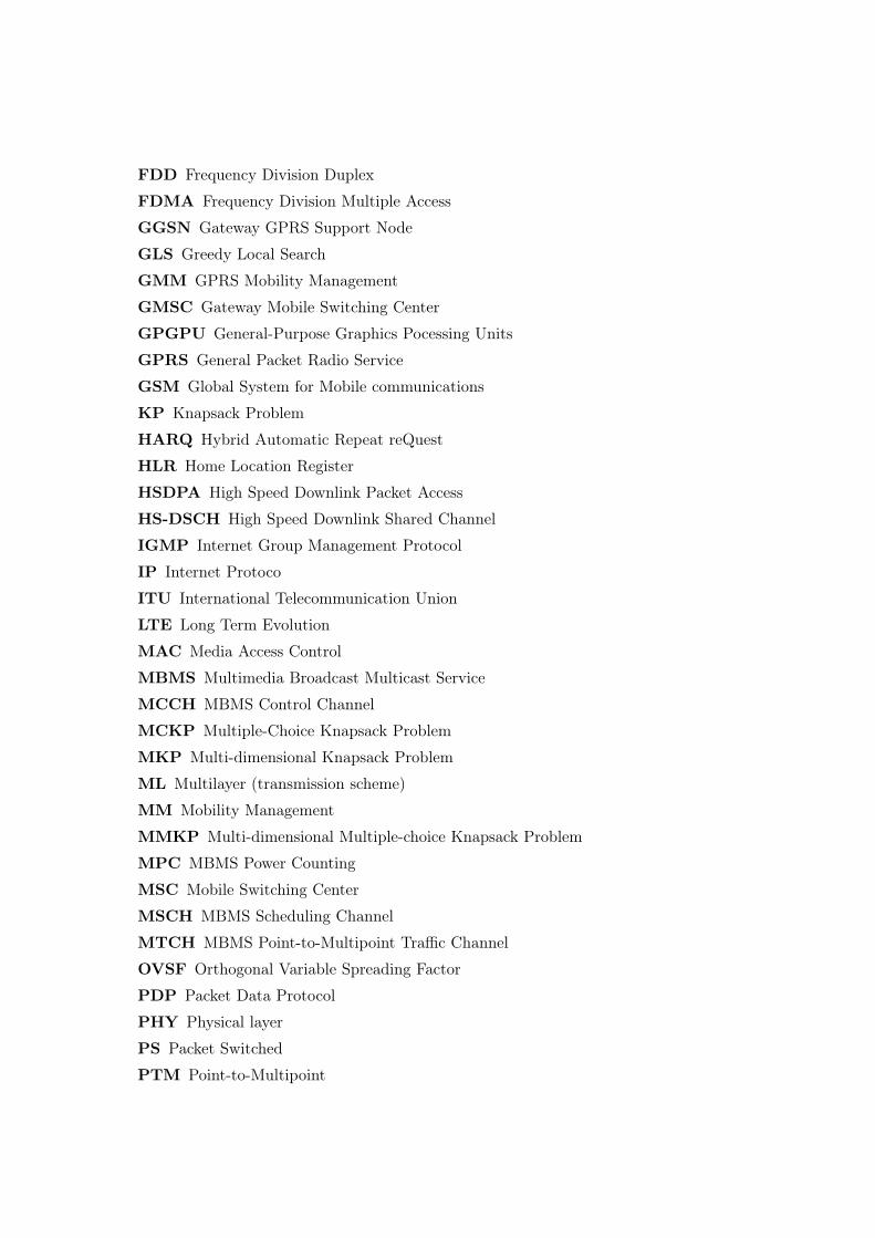
FDD Frequency Division Duplex
FDMA Frequency Division Multiple Access
GGSN Gateway GPRS Support Node
GLS Greedy Local Search
GMM GPRS Mobility Management
GMSC Gateway Mobile Switching Center
GPGPU General-Purpose Graphics Pocessing Units
GPRS General Packet Radio Service
GSM Global System for Mobile communications
KP Knapsack Problem
HARQ Hybrid Automatic Repeat reQuest
HLR Home Location Register
HSDPA High Speed Downlink Packet Access
HS-DSCH High Speed Downlink Shared Channel
IGMP Internet Group Management Protocol
IP Internet Protoco
ITU International Telecommunication Union
LTE Long Term Evolution
MAC Media Access Control
MBMS Multimedia Broadcast Multicast Service
MCCH MBMS Control Channel
MCKP Multiple-Choice Knapsack Problem
MKP Multi-dimensional Knapsack Problem
ML Multilayer (transmission scheme)
MM Mobility Management
MMKP Multi-dimensional Multiple-choice Knapsack Problem
MPC MBMS Power Counting
MSC Mobile Switching Center
MSCH MBMS Scheduling Channel
MTCH MBMS Point-to-Multipoint Traffic Channel
OVSF Orthogonal Variable Spreading Factor
PDP Packet Data Protocol
PHY Physical layer
PS Packet Switched
PTM Point-to-Multipoint

PTP Point-to-Point
QAM Quadrature Amplitude Modulation
QoS Quality of Service
RLC Radio Link Control
RNC Radio Network Controller
RNS Radio Network Subsystem
RRC Radio Resource Control
RRM Radio Resource Management
SA Simulated Annealing
S-CCPCH Secondary Common Control Physical Channel
SF Spreading Factor
SGSN Serving GPRS Support Node
SINR Signal to Interference Noise Ratio
SL Single Layer (transmission scheme)
SM Session Management
STTD Spatio-Temporal Transmit Diversity
TDMA Time Division Multiple Access
TFCI Transport Format Combination Indicator
TFI Transport Format Indicato
TS Tabu Search
TTI Transmission Time Interval
UE User Equipment
UMTS Universal Mobile Telecommunications System
USIM UMTS Subscriber Identity Module
UTRAN UMTS Terrestrial Radio Access Network
VLR Visitor Location Register
WCDMA Wideband Code Division Multiple Access


Appendix B
Appendix B: CQI mapping table
Table B.1: CQI mapping table [13]
CQI value Transport block size (bits) Num. of codes Modulation Total bit rate (kbps)
1 137 1 QPSK 480
2 173 1 QPSK 480
3 233 1 QPSK 480
4 317 1 QPSK 480
5 377 1 QPSK 480
6 461 1 QPSK 480
7 650 2 QPSK 960
8 792 2 QPSK 960
9 931 2 QPSK 960
10 1262 3 QPSK 1440
11 1483 3 QPSK 1440
12 1742 3 QPSK 1440
13 2279 4 QPSK 1920
14 2583 5 QPSK 1920
15 3319 5 QPSK 2400
16 3565 5 16-QAM 4800
17 4189 5 16-QAM 4800
18 4664 5 16-QAM 4800
19 5287 5 16-QAM 4800
20 5887 5 16-QAM 4800
21 6554 5 16-QAM 4800
22 7168 5 16-QAM 4800
23 9719 7 16-QAM 6720
24 11418 8 16-QAM 7680
25 14411 10 16-QAM 9600
26 17237 12 16-QAM 11520
27 21754 12 16-QAM 14400
28 23370 15 16-QAM 14400
29 24222 15 16-QAM 14400
30 25558 15 16-QAM 14400


Publication list during PhD study
Journal papers
Qing Xu, Frédéric Lassabe, Hakim Mabed, Alexandre Caminada, Fitness LandscapeAnalysis for Scalable Multicast RRM Problem in Cellular Network, In ElectronicNotes in Discrete Mathematics, ELSEVIER, Volume 41, Pages 407-414, ISSN 1571-0653.
International conference papers
(PIMRC 2014) Qing Xu, Hakim Mabed, Alexandre Caminada and Frédéric Lassabe,’Solving MBMS RRM Problem by Metaheuristics’, In 2014 IEEE 25th InternationalSymposium on Personal, Indoor and Mobile Radio Communications WashingtonDC, USA, 2-5 September, 2014.
(VTC 2014-Fall) Qing Xu, Hakim Mabed, Frédéric Lassabe and Alexandre Cam-inada, MBMS Radio Resource Optimization by Tabu Search, In 2014 IEEE 80thVehicular Technology Conference, Vancouver, Canada, 14-17 September, 2014.
(VTC 2013-Spring) Qing Xu, Hakim Mabed, Frédéric Lassabe and Alexandre Cam-inada, Optimization of Radio Resource Allocation for Multimedia Multicast in Mo-bile Networks, In 2013 IEEE 77th Vehicular Technology Conference, Dresden, Ger-many, 2-5 June 2013.
(WiOpt’13) Qing Xu, Hakim Mabed, Frédéric Lassabe and Alexandre Caminada,Modeling and Fitness Landscape Analysis for Flexible MBMS Radio Resource Allo-cation, In 11th International Symposium on Modeling and Optimization in Mobile,Ad Hoc, and Wireless Networks, Tsukuba Science City, Japan, 13-17 May, 2013.
National conference papers
(ROADEF’13) Qing Xu, Frédéric Lassabe, Hakim Mabed and Alexandre Caminada,Allocation par métaheuristique des ressources radio pour service de multi-diffusionhiérarchique, In 14e conference ROADEF de la société Française de RechercheOpérationnelle et Aide à la Décision, Troyes, France, 13-15 February, 2013.
(JDIR11) Qing Xu, Hakim Mabed, Frédéric Lassabe and Alexandre Caminada, ’Ef-

ficient Dynamic Radio Resource Management for Multimedia Broadcast MulticastServices’, In Proceedings of 10eme Journées Doctorales en Informatique et Réseaux,Belfort, France, 25 November, 2011.

Bibliography
[1] 3GPP TR 25.992 Multimedia Broadcast/Multicast Service (MBMS) ;UTRAN/GERAN requiremenst.
[2] 3GPP TR 30.03U Selection procedures for the choice of radio transmissiontechnologies of the UMTS.
[3] 3GPP TS 22.060 General Packet Radio Service (GPRS); Service description;Stage 1.
[4] 3GPP TS 23.060 General Packet Radio Service (GPRS); Service description;Stage 2,.
[5] 3GPP TS 25.211 Physical channels and mapping of transport channels ontophysical channels (FDD).
[6] 3GPP TS 25.213 Spreading and modulation (FDD).
[7] 3GPP TS 25.346 Introduction of the Multimedia Broadcast/Multicast Service(MBMS) in the Radio Access Network (RAN); Stage 2 (version 9.1.0 Release9).
[8] OPNET University Program: http://www.opnet.com /services/university/.
[9] 3rd Generation Partnership Project R1-021240 TSG-RAN WG128 Power Usagefor Mixed FACH and DCH for MBMS, 2002.
[10] 3GPP TS 23.041: Technical Realization of Cell Broadcast Service (CBS), Jan.2004.
[11] Usage of link-level performance indicators for HSDPA network-level simulationsin E-UMTS, Sydney, Australia, 2004. Proceedings of IEEE ISSSTA 04.
[12] 3GPP TR 25.803 S-CCPCH performance for MBMS25.922, September 2005.
[13] 3GPP TS 25.214 Physical layer procedures (FDD), June 2005.
[14] 3GPP TS 25.324 Broadcast/Multicast Control (BMC), June 2006.
[15] 3GPP TR 25.922 Radio resource management strategies, March 2007.
[16] 3GPP TS 23.246 Multimedia Broadcast/Multicast Service (MBMS); Architec-ture and functional description (Release 6), June 2007.
[17] 3GPP TS 23.246 Multimedia Broadcast/Multicast Service (MBMS); Architec-ture and functional description (Release 7), September 2007.
[18] 3GPP TS 25.346 Introduction of the Multimedia Broadcast/Multicast Service(MBMS) in the Radio Access Network (RAN); Stage 2, March 2011.
[19] UMTS Forum Summary of Recent Activities. Technical report, UMTS Forum,2011.
[20] VNI mobile forecast highlights 2012 - 2017, 2013.
[21] A. Alexiou, C. Bouras, and V. Kokkinos. An enhanced MBMS power con-trol mechanism towards long term evolution. In Wireless TelecommunicationsSymposium, 2009. WTS 2009, pages 1–6, April 2009.
[22] A. Alexiou, C. Bouras, V. Kokkinos, and E. Rekkas. MBMS power planning inmacro and micro cell environments. In 12th IEEE Symposium on Computersand Communications, (ISCC 2007), pages 33– 38, July 2007.
[23] Antonios Alexiou, Christos Bouras, and Vasileios Kokkinos. Evaluation of dif-ferent power saving techniques for MBMS services. EURASIP Journal on Wire-less Communications and Networking, pages 1–15, January 2009.
[24] Antonios Alexiou, Christos Bouras, and Evangelos Rekkas. A power controlscheme for efficient radio bearer selection in MBMS. In IEEE InternationalSymposium on a World of Wireless, Mobile and Multimedia Networks, pages1–8, June 2007.
[25] Antonios Alexiou, Christos Bouras, and Evangelos Rekkas. An improved mbmspower counting mechanism towards long term evolution. TelecommunicationSystems, 43(1-2):109–119, 2010.
[26] Cristina Bazgan, Hadrien Hugot, and Daniel Vanderpooten. Solving efficientlythe 0-1 multi-objective knapsack problem. Computers and Operations Research,36(1):260 – 279, 2009.
[27] Christian Blum and Andrea Roli. Metaheuristics in combinatorial optimization:Overview and conceptual comparison. ACM Computing Surveys, 35(3):268–308, September 2003.
[28] Christophoros Christophorou, Andreas Pitsillides, and Tomas Lundborg. En-hanced radio resource management algorithms for efficient mbms service pro-vision in UTRAN. Computer Networks, 55(3):689–710, 2011.
[29] PC Chu and JE Beasley. A genetic algorithm for the multidimensional knapsackproblem. Joural of Heuristics, 4(1):63–86, Jun 1998.
[30] T.H. Cormen, C.E. Leiserson, R.L. Rivest, and C. Stein. Introduction To Al-gorithms. MIT Press, 2001.
[31] Amrico M. C. Correia, Joo C. M. Silva, Nuno M. B Souto, Lusa A. C.Silva, Alexandra B. Boal, and Armando B. Soares. Multi-resolution broad-cast/multicast systems for MBMS. IEEE Transactions on Broadcasting,53(1):224–234, March 2007.
[32] P.J. Czerepinski, T.M. Chapman, and J. Krause. Coverage and planning aspectsof MBMS in UTRAN. In Fifth IEE International Conference on 3G MobileCommunication Technologies, 2004.
[33] I. De Falco, R. Del Balio, E. Tarantino, and R. Vaccaro. Improving search byincorporating evolution principles in parallel Tabu Search. In Proceedings of theFirst IEEE Conference on Evolutionary Computation, IEEE World Congresson Computational Intelligence,, pages 823–828 vol.2, Jun 1994.

[34] Isabelle Devarenne, Hakim Mabed, and Alexandre Caminada. Adaptive tabutenure computation in local search. In Jano Hemert and Carlos Cotta, edi-tors, Evolutionary Computation in Combinatorial Optimization, volume 4972of Lecture Notes in Computer Science, pages 1–12. Springer Berlin Heidelberg,2008.
[35] M.M. Diallo, Samuel Pierre, and R. Beaubrun. A tabu search approach forassigning node bs to switches in umts networks. IEEE Transactions on WirelessCommunications, 9(4):1350–1359, April 2010.
[36] R.W. Eglese. Simulated annealing: A tool for operational research. EuropeanJournal of Operational Research, 46(3):271 – 281, 1990.
[37] France Telecom University of Surrey RWTH Aachen RAI Ericsson, Motorola.IST-2001-35125, Deliverable of the project (D08), Spectrum efficient multicastand asymmetric servicesin UMTS. Technical report, 2003.
[38] Thomas Erlebach, Hans Kellerer, and Ulrich Pferschy. Approximating multi-objective knapsack problems. In Algorithms and Data Structures, Lecture Notesin Computer Science, pages 210–221. Springer Berlin Heidelberg, 2001.
[39] Cyril Fonlupt, Denis Robilliard, Philippe Preux, and El-Ghazali Talbi. Fitnesslandscapes and performance of meta-heuristics. In Meta-Heuristics: Advancesand Trends in Local Search Paradigms for Optimization, page 257268. KluwerAcademic Publishers, 1999.
[40] Arnaud Fréville. The multidimensional 01 knapsack problem: An overview.European Journal of Operational Research, 155(1):1 – 21, 2004.
[41] M. Garland. Parallel computing with cuda. In Parallel Distributed Processing(IPDPS), 2010 IEEE International Symposium on, pages 1–1, April 2010.
[42] Stuart Geman and D. Geman. Stochastic relaxation, gibbs distributions, andthe bayesian restoration of images. IEEE Transactions on Pattern Analysis andMachine Intelligence, PAMI-6(6):721–741, Nov 1984.
[43] Fred Glover. Future paths for integer programming and links to artificial intel-ligence. Computers and Operations Research, 13(5):533 – 549, 1986.
[44] Fred Glover. Tabu search part I. ORSA Journal on computing, 1(3):190–206,1989.
[45] Fred W. Glover and Gary A. Kochenberger, editors. Handbook of Metaheuris-tics. Springer, 1st edition, January 2003.
[46] Gurobi Optimization. Gurobi Optimizer Reference Manual, December 2009.[47] Hans-Otto Gunther and Kap Hwan Kim. Container terminals und cargo sys-
tems: design, operations management, and logistics control issues. Springer,Berlin, 2007.
[48] H. Hamacher. Theoretical and computational aspects of simulated annealing:Theory and applications. SIAM Review, 32(3):504–506, 1990.
[49] Antti Toskala Harri Holma. HSDPA/HSUPA for UMTS: High Speed RadioAccess for Mobile Communications. John Wiley and Sons, 2006.

[50] S. Mehdi Hashemi, Mohsen Rezapour, and Ahmad Moradi. Two new algo-rithms for the min-power broadcast problem in static ad hoc networks. AppliedMathematics and Computation, 190(2):1657 – 1668, 2007.
[51] Mariann Hauge. Multicast in 3G networks: Employment of existing IP multi-cast protocols. pages 96–103, 2002.
[52] Cornelius Hellge, Thomas Schierl, Jörg Huschke, Thomas Rusert, MarkusKampmann, and Thomas Wiegand. Graceful degradation in 3GPP MBMSmobile TV services using H.264/AVC temporal scalability. EURASIP Journalon Wireless Communications and Networking, 2009:207210, 2009.
[53] Harri Holma and Antti. Toskala. WCDMA for UMTS: Radio Access for ThirdGeneration Mobile Communications. Wiley, 2000.
[54] Harri Holma and Antti Toskala. WCDMA for UMTS: HSPA Evolution andLTE. Wiley Online Library: Books. Wiley, 2010.
[55] IST-2003-507607 (B-BONE). Final results with combined enhancements of theair interface, deliverable of the project (D2.5). Technical report.
[56] A. Van Ewijk J. De Vriendt, I. Gomez Vinagre. Multimedia broadcast and mul-ticast services in 3G mobile networks. Technical Report 4-1, Alcatel Telecom-munications Review, 2004.
[57] Kil-Woong Jang. A tabu search algorithm for routing optimization in mobilead-hoc networks. Telecommunication Systems, 51(2-3, SI):177–191, NOV 2012.
[58] A. Janiak, W. ladys law Janiak, and M. Lichtenstein. Tabu search on GPU.Journal of Universal Computer Science, 14(14):24162427, 2008.
[59] Hany Kamal, Marceau Coupechoux, and Philippe Godlewski. Tabu searchfor dynamic spectrum allocation in cellular networks. IEEE Transactions onEmering Telecommunications Technologies, 23(6):508–521, oct 2012.
[60] Richard M. Karp. Reducibility among combinatorial problems. In R. E. Millerand J. W. Thatcher, editors, Complexity of Computer Computations, page85103. Plenum, New York, 1972.
[61] S. Kirkpatrick, C. D. Gelatt, and M. P. Vecchi. Optimization by simulatedannealing. Science, 220:671–680, 1983.
[62] The Van Luong, N. Melab, and E.-G. Talbi. Gpu computing for parallel localsearch metaheuristic algorithms. Computers, IEEE Transactions on, 62(1):173–185, Jan 2013.
[63] Hakim Mabed, Alexandre Caminada, and Jin-Kao Hao. Genetic Tabu searchfor robust fixed channel assignment under dynamic traffic data. ComputationalOptimization and Applications, 50(3):483–506, DEC 2011.
[64] Raïd Mansi, Cláudio Alves, J. M. Valério de Carvalho, and Saïd Hanafi. Ahybrid heuristic for the multiple choice multidimensional knapsack problem.Engineering Optimization, 45(8):983–1004, 2013.

[65] A. Medeisis and A. Kajackas. On the use of the universal okumura-hata prop-agation prediction model in rural areas. In Vehicular Technology ConferenceProceedings, (VTC-Spring) Tokyo., volume 3, pages 1815–1818 vol.3, 2000.
[66] Peter Merz and Bernd Freisleben. Fitness landscapes and memetic algorithmdesign. In New Ideas in Optimization, pages 245–260. McGraw-Hill, 1999.
[67] S. Parkvall, E. Englund, M. Lundevall, and J. Torsner. Evolving 3g mobile sys-tems: broadband and broadcast services in wcdma. Communications Magazine,IEEE, 44(2):30–36, Feb 2006.
[68] A. Raschella, A. Umbert, G. Araniti, A. Iera, and A. Molinaro. SINR-Basedtransport channel selection for mbms applications. In IEEE 69th VehicularTechnology Conference, (VTC Spring) 2009, pages 1–5, April 2009.
[69] C. R. Reeves. Modern Heuristic Techniques for Combinatorial Problems. JohnWiley & Sons, 1 edition, April 1993.
[70] Jordi Perez Romero, Oriol Sallent, Ramon Agusti, and Miguel Angel Diaz-Guerra. Radio Resource Management Strategies in UMTS. Wiley, 1 edition,August 2005.
[71] Said Salhi. Defining tabu list size and aspiration criterion within tabu searchmethods. Computers and Operations Research, 29(1):67–86, 2002.
[72] Jochen H Schiller. Mobile Communications. Addison-Wesley, London, 2011.
[73] Luísa Silva and Américo Correia. Hsdpa delivering MBMS video streaming.In Proceedings of the 2006 ACM CoNEXT Conference, CoNEXT ’06, pages20:1–20:2, New York, NY, USA, 2006. ACM.
[74] Prabhakant Sinha and Andris A. Zoltners. The multiple-choice knapsack prob-lem. Operations Research, 27(3):503–515, 1979.
[75] PeterF. Stadler and SantaFe Institute. Towards a theory of landscapes. InComplex Systems and Binary Networks, volume 461-461 of Lecture Notes inPhysics, pages 78–163. Springer Berlin Heidelberg, 1995.
[76] B. Suman and P. Kumar. A survey of simulated annealing as a tool for singleand multiobjective optimization. Journal of the Operational Research Society,57(18):1143–1160, 2006.
[77] Harold Szu and Ralph Hartley. Fast simulated annealing. Physics Letters A,122(34):157 – 162, 1987.
[78] Lucent Technologies. 3GPP TSG RAN WG1 No.29; R1-02-1324; Power Controlfor FACH, November 2002.
[79] Lucent Technologies. TSG-RAN WG1 No.33 r1-030778; Rate Splitting forMBMS, August 2003.
[80] V. Vartiainen and J. Kurjenniemi. Point-to-multipoint multimedia broadcastmulticast service (MBMS) performance over HSDPA. In IEEE 18th Inter-national Symposium on Personal, Indoor and Mobile Radio Communications,(PIMRC 2007), pages 1–5, 2007.

[81] Kun Wang, Fan Yang, Qian Zhang, Dapeng Oliver Wu, and Yinlong Xu. Dis-tributed cooperative rate adaptation for energy efficiency in IEEE 802.11-basedmultihop networks. IEEE Transactions on Vehicular Technology, 56(2):888–898, MAR 2007.
[82] S. Wright. The roles of mutation, inbreeding, crossbreeding and selection inevolution. In Proc of the 6th International Congress of Genetics, volume 1,page 356366, 1932.
[83] V. erný. Thermodynamical approach to the traveling salesman problem: An ef-ficient simulation algorithm. Journal of Optimization Theory and Applications,45(1):41–51, 1985.