www.elsevier.com/locate/comcom

Computer Communications 30 (2006) 101–116

Landscape analysis for multicast routing

M.S. Zahrani a, M.J. Loomes b, J.A. Malcolm a, A.A. Albrecht a,*

a University of Hertfordshire, School of Computer Science, Hatfield, Herts AL10 9AB, UKb Middlesex University, School of Computing Science, Hendon, London NW4 4BT, UK

Received 9 June 2006; received in revised form 27 July 2006; accepted 28 July 2006Available online 28 August 2006

Abstract

In recent years, methods based on local search have been utilized in off-line algorithms for multicast routing in communication net-works. In multicast routing, several point-to-multipoint requests have to be scheduled under constraints associated with each link of theunderlying network such as capacity and transmission costs. We propose a landscape analysis technique to solve this problem, whereeach particular request is routed by a Steiner tree heuristic. The landscape analysis employs simulated annealing with a logarithmic cool-ing schedule, which has been proved to be an appropriate tool to tackle hard problems from Combinatorial Optimisation and Compu-tational Biology. We present results from computational experiments performed on three instances from the OR library. Emphasis isplaced on algorithmic aspects of off-line routing, in particular, on approximations of optimal parameter settings, rather than on imple-mentations of fast online network protocols. Furthermore, we investigate the impact of capacity noise on parameter settings and we per-form a comparison to genetic algorithms based upon PMX crossover.� 2006 Elsevier B.V. All rights reserved.

Keywords: Multicast routing; Landscape analysis; Simulated annealing; Steiner trees; Quality of service (QoS)

1. Introduction

The multicast (point-to-multipoint) routing problem incommunication networks is a real business problem thatrequires an efficient solution to ensure the viability of largecommunication networks. In recent years, great effort hasbeen undertaken to introduce and incorporate quality ofservice (QoS) into data communication networks such asATM and IP networks [1–8]. Many multicast applications,such as video conferencing, distance-learning, and multi-media broadcasting are QoS-sensitive in nature and thusthey will all benefit from the QoS support of the underlyingnetworks. The challenge is how to build multicast trees todeliver the multicast data from each source to the appropri-ate receivers in such a way that QoS requirements are sat-isfied and the demand for network resources is minimised.

0140-3664/$ - see front matter � 2006 Elsevier B.V. All rights reserved.

doi:10.1016/j.comcom.2006.07.019

* Corresponding author. Tel.: +44 1707 284 247; fax: +44 1707 284 303.E-mail address: A.Albrecht@herts.ac.uk (A.A. Albrecht).

Designing multicast routing algorithms is a complex andchallenging task [3] with many different aspects. Among thevarious issues involved are the design of optimal routestaking into consideration different cost functions, the mini-misation of network load and the avoidance of loops andtraffic congestion, and the provision of basic support forreliable transmission. In the present paper, we focus onthe design of optimal routes.

The problem of minimizing the tree costs of singlerequests under the constraint that all path capacities arewithin a user-specified capacity bound is referred to asthe capacity constrained multicast routing problem. Foran overview of multicast routing algorithms and particularmethods for tackling the multicast routing problem werefer the reader to [3,9–12]. In [11], for example, a combi-nation of multiple shared trees with anycast routing is pro-posed, where anycast routing is executed to nearest nodesin shared trees that are induced by the multicast task.The algorithm is designed for fast and efficient onlineInternet routing and utilizes a fast heuristic for setting-up

102 M.S. Zahrani et al. / Computer Communications 30 (2006) 101–116

a minimum Steiner tree. The minimum Steiner tree prob-lem is known to be NP-complete [13], which implies theNP-completeness of the more general multicast routingproblem. We note that in applications like video conferenc-ing, multimedia broadcasting, and distance-learning therouting procedure is updated only from time to time,e.g., when new customers register to use one of the services.In such cases, off-line routing algorithms are a possible wayto solve the multicast routing problem, which is in contrastto online updates where fast methods are required [14].

Since we are dealing with an NP-complete problem,local search methods are a natural choice to tackle theproblem. Various applications of search-based methodsto the multicast routing problem are presented in [15–19].In our paper, we focus on a specific type of simulatedannealing [20–24]. This search method has been employedbefore in the context of (multicast) routing [25–30], in par-ticular under QoS considerations. In [25], the QoS issue isreduced to a path constraint problem, where along a pathfrom source to destination each link has to obey a vector ofweight restrictions. The constraint vector is transformedinto an energy function by a max-operation over the com-ponent-wise ratio of link weights and capacity constraints.The search for appropriate paths is then executed by simu-lated annealing. The paper [26] demonstrates how differentQoS requirements like available CPU resources, bufferresources, error rates, queuing delay, and sending delayat each node as well as available bandwidth, transmissiondelay, and error rate at each link can be incorporated intoa single energy function for a given potential multicastrouting solution. Simulated annealing is then applied tothis energy function, where the underlying model is ahomogeneous Markov chain (cf. Section 4.1). Since thespecific QoS requirements considered in [26] do not affectthe general methodology, we have chosen only two QoSparameters for the calculation of the energy function(cf. Section 2). In [29] (see also [6]), an overlay multicastnetwork infrastructure is proposed which forms a multicastdata delivery backbone. The overlay topology is continu-ously adapted (off-line) with changes in the distributionof the clients as well as changes in network conditions.The performance optimisation is executed by a simulatedannealing-based algorithm defined by homogeneous Mar-kov chains. The paper [30] employs a QoS setup similarto [26] and investigates three different search methods: sim-ulated annealing, tabu search, and genetic algorithms. Thethree methods are tested on small (14 nodes, 21 edges) andrelatively large (100 nodes, 800 edges) randomly generatednetworks. The findings suggest that simulated annealingcan solve multicast routing problems efficiently with high-quality solutions, tabu search-based algorithms show agood time performance when the group size is large, andthat GA genetic-based methods slightly outperform SA interms of the solution quality.

In the present paper, we introduce the concept of land-scape analysis to the problem of multicast routing. Thenotion of landscape analysis was first mentioned in [31]

and has become a major topic in combinatorial optimisa-tion in recent years [32–34]. Our tool for landscape analysisis logarithmic simulated annealing (LSA) [22,23,35], i.e. inour approach we employ simulated annealing based oninhomogeneous Markov chains. Recently, simulatedannealing algorithms, in particular variants based on inho-mogeneous Markov chains, have been used to investigateproblems from Computational Biology [36,37]. Anothermotivation for choosing simulated annealing is based uponrecent advances in genetic algorithms research [38]: L.M.Schmitt proved that in order to ensure the convergenceof genetic algorithms to optimum solutions, simulatedannealing-based selection has to be employed in one wayor another (see Section 10 in [38] for a summary of results).Since we focus on algorithmic aspects of multicast routingin off-line mode, we reduce the QoS requirements to band-width and delay constraints (cf. preceding paragraph). Themain aim is to demonstrate the performance of LSA andhow to extract landscape parameters. Furthermore, weinvestigate how bandwidth noise may affect the landscapeparameters. The present paper is an extension of [39],where we showed that LSA outperforms genetic algorithmsbased on PMX crossover. The competitiveness of LSA inrelation to genetic algorithms and tabu search was demon-strated in [40] for the job shop scheduling problem, whichis one of the hardest NP-complete problems.

The paper is structured as follows: in Section 2, we pro-vide a formal definition of the multicast routing problem,along with explanations about parameters and cost func-tions. Section 3 reviews briefly the approach by Zhu et al.[15] which is used in our neighbourhood function. In Sec-tion 4, simulated annealing is introduced in the contextof multicast routing, with particular emphasis on inhomo-geneous Markov chains. In Section 5, we present resultsfrom computational experiments performed on threeinstances from the OR library [41] modified for multicastrouting. The instances have 75–100 nodes and 150–200edges. The experiments were executed on several sets ofrequests, and we provide detailed information about therequests, including cost parameters and link capacities.We propose a way to estimate crucial parameters of thecooling schedule, and we compare the results of runsperformed for different parameter settings. The outcomeconfirms the efficacy of our approach to estimate specificcharacteristics of the energy landscape induced bysimulated annealing-based search.

2. Formal definition of multicast routing

Communication networks consist of nodes connectedthrough links. The nodes are the originators and receiversof information, while the links serve as the transportbetween nodes. Nodes can be either endpoint nodes orintermediary nodes. Both nodes and links have a limitedcapacity of information flow they can handle, dependingon features such as speed of information flow and thecost of transferring the information at the required speed.

M.S. Zahrani et al. / Computer Communications 30 (2006) 101–116 103

The problem of multicast routing is a complex one. Thenaıve approach to solving the point-to-multipoint routingproblem is through the separation of the problem into sev-eral point-to-point routing problems according to the num-ber of destination points. This simple method is veryinefficient: the same information might flow on the samelink many times. It creates unnecessary traffic on the link,which could be avoided. Therefore, we use another formal-isation where messages from a single source are combinedto form a single request.

In our formal definition of multicast routing we follow[15,17]: given a graph G = (V,E) that represents a commu-nication network with node set V and edges E, we definetwo non-negative weight functions Co : E! R andCa : E! R, where Co is the cost function and Ca thecapacity function on E, respectively.

Each of the point-to-multipoint requests has a sourcenode s 2 V and a set of destination nodes D ˝ V. We definea multicast request R by setting

R¼½vs)ðv1;v2;...;vnÞ;C�; where

vs¼the source node of R;

D¼fv1;...;vng¼ the destination nodes;

C¼the capacity required by each of the transmissions vs)vi:

ð1Þ

The multicast problem P is then defined by

P ¼ ½G; Co; Ca; R1; . . . ;Rn�: ð2Þ

Fig. 1. Genetic algori

Usually, multicast routing algorithms are based on the fol-lowing assumptions [3,15,17,18]. Each R from P is routedseparately by a minimum Steiner tree with root vs andleaves D. The cost of the Steiner tree is the sum

PeCoðeÞ

of the costs of the edges in the tree, while the capacityCa(e) on each edge on a path from vs to each vi 2 D obeysCa(e) P C for C defined by R, see (1).

However, to minimiseP

eCoðeÞ for given G, vs, D, Co,and Ca is NP-complete [13]. Numerous heuristics havebeen devised to find good approximations of minimumsolutions efficiently [42–46]. Since in our approach singlerequests may have to be rerouted many times in order tosatisfy capacity constraints, we employ the simple but effi-cient KMB algorithm [43]. It has been estimated that thecost of a tree generated with the KMB algorithm averages5% more than the cost of a Steiner minimal tree [14]. Thealgorithm proposed in [46] implies that each request canbe routed in polynomial time within 5/3 of the minimumcost of a Steiner tree. Koch and Martin [45] obtained min-imum values for a large number of benchmark problems byusing a polyhedral method. Of course, the KMB algorithmwe are using can be substituted by any efficient Steiner treealgorithm.

3. Genetic algorithms for multicast routing

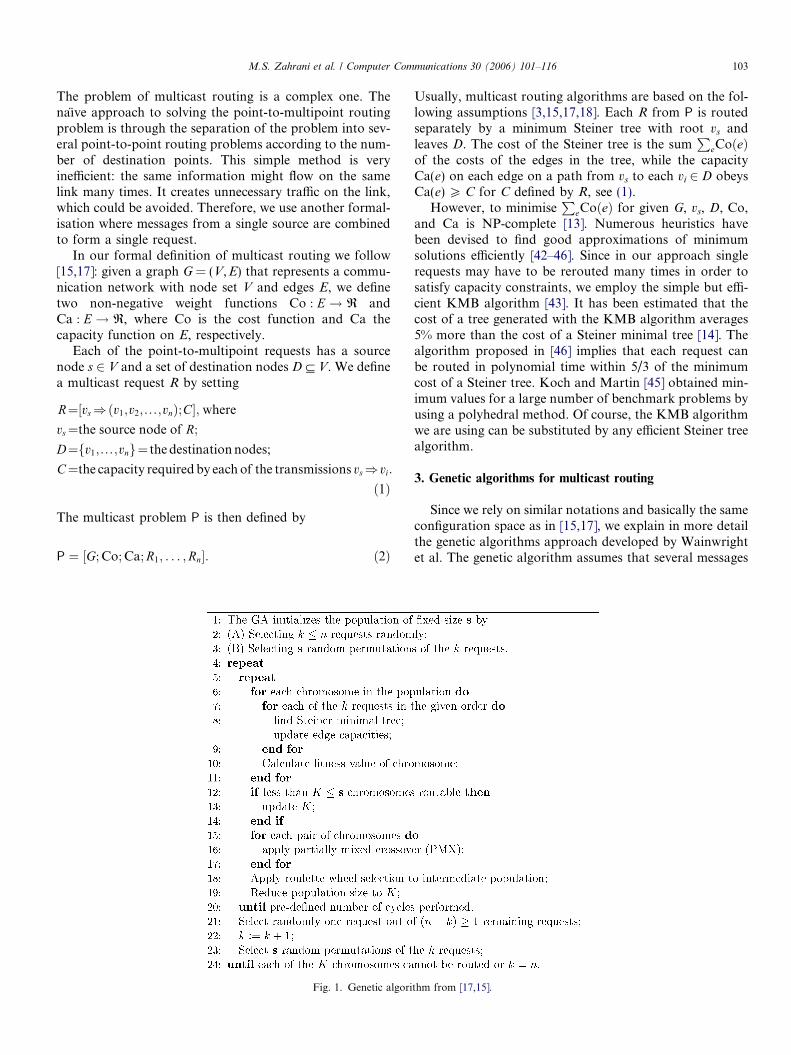
Since we rely on similar notations and basically the sameconfiguration space as in [15,17], we explain in more detailthe genetic algorithms approach developed by Wainwrightet al. The genetic algorithm assumes that several messages

thm from [17,15].

104 M.S. Zahrani et al. / Computer Communications 30 (2006) 101–116

are transferred from several sources into multiple destina-tions simultaneously, without any order or priority for cer-tain messages. The algorithm uses a population ofchromosomes, where each chromosome is a permutationof the numbers that are assigned to the requests (permuta-tions of length n, cf. (2)). Actually, the genetic algorithmstarts with a subset of k out of n requests only. By usinga Steiner tree algorithm, the k requests are routed in theorder they appear in the chromosome (partial permuta-tion). The fitness value assigned to the chromosome takesinto account the cost function Co as given in (1) and (2).

The algorithm starts with a randomly chosen popula-tion. The partially mixed crossover (PMX) is applied topairs of chromosomes [47]: two strings are aligned andtwo crossing sites are picked uniformly at random alongthe strings. The positions P1 and P2 define a matching sec-tion where the requests are exchanged position by position.This operation may generate duplicate occurrences ofrequests, therefore, the following procedure is applied tothe rest of the positions (outside the matching section): ifR has a duplicate R 0 in the same string (offspring-1), thenthe duplicate R 0 outside the matching region is substitutedby the request R00 from the other offspring (offspring-2) thatwas swapped with R. This guarantees that each request isfound exactly once in the offspring. The new population(of the same fixed size) is then generated by roulette wheelselection, where a sector of a ‘‘roulette wheel’’ is assignedto each offspring, whose size is proportional to the fitnessmeasure, and then a random position is chosen on thewheel (see Fig. 1).

The algorithm runs a fixed number of steps, and then k

is increased by one in order to check whether (k + 1)requests can be scheduled conflict-free, i.e. the sameprocedure is repeated for (k + 1) etc. until either k = n orrepeated attempts to schedule simultaneously k requestsare unsuccessful.

In [15], the population size is 100 and 100 crossover/se-lection steps are executed for each k 6 n. The n = 20requests were defined in a network with 61 nodes and133 edges. Each request R has at least eight destinationnodes, and the capacity C was between five and nine; see(1). Feasible solutions were found for k 6 18. Since the net-work information is not provided in detail, we are unfortu-nately unable to apply our approach to the multicastrouting example analysed in [15].

4. A simulated annealing-based approach

Simulated annealing was introduced as an optimisationtool independently in [20] and [21]; see also [24]. The under-lying algorithm acts within a configuration space in accor-dance with a specific neighbourhood structure, where thetransition steps are controlled by the objective function.Unlike applications of simulated annealing to multicastrouting as presented, e.g., in [25–30], we focus on simulatedannealing based on inhomogeneous Markov chains, asexplained in the next section.

4.1. Basics of simulated annealing in the multicast routing

context

The configuration space consists of all feasible solutionsfor a given multicast problem P = [G; Co; Ca; R1,. . .,Rn].We denote the configuration space by

M ¼ fS j S ¼ ½Ri1 ; . . . ;Rin �; Ri1 ; . . . ;Rin are SMT-routedg:ð3Þ

Here, SMT-routed means that each Rij from the ordered se-quence S is routed by the KMB algorithm [43] that approx-imates a Steiner minimal tree (SMT).

By NS we denote the neighbourhood of S, and Z(S) isthe underlying objective function. Both objects are speci-fied later in Section 4.2. The neighbours NS are all requiredto be feasible solutions.

The probability of performing a transition from S toS 0 2 NS is defined by

PrfS ! S0g ¼G½S; S0� � A½S; S0� if S0 6¼ S;

1�P

H 6¼SG½S;H � � A½S;H �; otherwise;

8<:

ð4Þwhere G[S,S 0] and G[S,H] are the probabilities of generat-ing multicast routing solutions S 0 and H, respectively,where S 0,H 2 NS, and A is the probability of acceptingthe neighbour once it has been generated according to G.

In an ‘‘ideal’’ setting, the generation probability is uni-form and defined by

G½S; S0� :¼1jNS j if S0 2 N S ;

0; otherwise:

(ð5Þ

The ‘‘uniform’’ definition assumes that all potential neigh-bours are tested whether they are feasible or not in orderto determine NS and jNSj, which would require a large num-ber of SMT calculations. In the actual implementation (seeSection 5), a potential neighbour is chosen randomly and itsfeasibility is tested. If conflicts arise in simultaneous sched-uling, a new potential neighbour is chosen; see Section 4.2.

The acceptance probabilities A[S,S 0], S 0 2 NS, arederived from the underlying analogy to thermodynamicsystems:

A½S; S0� :¼1 if ZðS0Þ � ZðSÞ 6 0;

e�ðZðS0Þ�ZðSÞÞ=c; otherwise;

�ð6Þ

where c is a control parameter having the interpretation ofa temperature in annealing procedures. The actual deci-sion, whether or not S 0 should be accepted in case ofZ(S 0) > Z(S), is performed in the following way: S 0 isaccepted, if

e�ðZðS0Þ�ZðSÞÞ=c P q; ð7Þ

where q 2 [0,1] is produced by a random numbergenerator. The value q is generated in each trial in caseof Z(S 0) > Z(S).

5

1

42

7

3

4

1

3

2

7

5

Fig. 2. A neighbourhood transition example.

M.S. Zahrani et al. / Computer Communications 30 (2006) 101–116 105

Let aS(k) denote the probability of being in configura-tion S 2M after k steps according to (4)–(7). The probabil-ity aS(k) is given by

aSðkÞ :¼X

H

aH ðk � 1Þ � PrfH ! Sg; ð8Þ

where Pr{H fi S} is from (4). The recursive application of(8) defines a Markov chain of probabilities aS(k), whereS 2M and k = 1,2, . . . If the parameter c = c(k) in (6) isa constant c, the chain is said to be a homogeneous Mar-kov chain; otherwise, if c(k) is lowered at each step, the se-quence of probability vectors ~aðkÞ is an inhomogeneousMarkov chain.

We consider only one special type of inhomogeneousMarkov chains. The motivation for this choice is basedupon the convergence properties of the two types of Mar-kov chain: convergence propositions about homogeneousMarkov chains rely on an infinite number of transitionsat fixed ‘‘temperatures’’ c. The probability distributionapproached in the limit is the Boltzmann distributione�Z(S)/c/F, where F is a normalisation value. If c fi 0, theBoltzmann distribution tends to the distribution over opti-mum configurations. In practice, however, it is infeasible toperform an infinite number of transitions at fixed tempera-tures, and this explains why this type of simulated anneal-ing with cooling heuristics is usually stuck in local minima.The convergence analysis of inhomogeneous Markovchains avoids the intermediate step, and in our approachthe ‘‘temperature’’ c(k) changes in accordance with

cðkÞ ¼ Clnðk þ 2Þ ; k ¼ 0; 1; . . . ð9Þ

The choice of c(k) is motivated by Hajek’s theorem [22] onlogarithmic cooling schedules. We denote by Fmin the set ofoptimum solutions. Basically, Hajek’s theorem states

Theorem 1. [22] Under some natural assumptions about the

configuration space F and the neighbourhood relation Nf, the

asymptotic convergenceXf2F min

af ðkÞk!1�!1 ð10Þ

of logarithmic simulated annealing is guaranteed if and only

if C from (9) is lower bounded by the maximum value of the

minimum escape height from local minima.

Unfortunately, due to the complex nature of our configura-tion space M, we are not in the position to decide whetheror not Theorem 1 applies. However, logarithmic simulatedannealing has proved to be an efficient method in similarsettings; see [40].

4.2. Neighbourhood and objective function

There are numerous ways to define the neighbourhoodrelation; in the present study, we focus on one example only.Given S 2M by S ¼ ½Ri1 ; . . . ;Rin �, the neighbourhood NS

includes S itself and is defined by the following procedure:

Two integers a and b, where 1 6 a < b 6 n, are random-ly chosen, and the order of all requests from number iato number ib is reversed. Thus, a new potential configu-ration S 0 is generated (see Fig. 2).The potential configuration S 0 is validated for feasibili-ty, i.e. we try to simultaneously schedule all the requestsfrom Rib

upwards. If a conflict occurs, a new pair (a,b) isgenerated.If S 0 indeed belongs to M, the objective function Z(S) iscalculated.

In [26,30], various QoS constraints are taken intoaccount in order to define the objective function: everynode v 2 V is labelled by the following parameters: avail-able CPU resources c(v), available buffer resources b(v),queuing delay t(v), and sending delay s(v). Furthermore,every link e = (v,u) is labelled by: available bandwidthw(e) and transmission delay d(e). The QoS constraints arethen given by

8vðcðvÞP C; bðvÞP B; wðeÞP W Þ ð11Þfor some constants C,B and W, where additionally thesource-destination delay, calculated from t(v), s(v) andthe sum of d(e), is bounded by D. The task is to minimizea function ð

PvhðvÞ þ

PeHðeÞ þ QÞ, where h and H are

heuristic cost functions and Q is the weighted number ofsource-destination pairs that violate the delay bound; h

and H are defined by

hðvÞ :¼ j1

cðvÞ þj2

bðvÞ ; HðeÞ :¼ j3

wðeÞ ð12Þ

for some constants j1,j2 and j3. Thus, the QoS constraintsare incorporated into a single additive function. Since weare interested in algorithmic aspects, i.e. the presentationof a landscape approach based on logarithmic simulatedannealing, we consider a simplified version of the objectivefunction. Moreover, in contrast to, e.g., [26,30] we considerthe simultaneous routing of several requests (ranging from9 to 20 in our experiments, see Section 5). Our cost functionCo can represent, e.g., the delay along a single link, and thecapacity Ca can be related to the bandwidth. In our setting,feasible solutions have to obey the bandwidth constraints,

106 M.S. Zahrani et al. / Computer Communications 30 (2006) 101–116

and adding c(v), b(v), t(v) and s(v) to the selection of feasi-ble solution would not change the overall approach.

Our objective function is basically chosen as in [15,17]and represents a combined measure of transmission costsand capacity constraints: let T(R) denote the set of edgesof the tree associated with the request R from configurationS 2M. We first define

W ðRÞ :¼ C �X

e2T ðRÞCoðeÞ; ð13Þ

where Co is from (2) and C the capacity request of R; see(1). The value of the objective function Z(S), S 2M, is thensimply given by

ZðSÞ :¼X

R from S

W ðRÞ: ð14Þ

4.3. Calculation of initial feasible solutions

We randomly select an order (i1, i2 , . . ., in) ofij 2 [1,2, . . .,n]. If the request Rij has been scheduled suc-cessfully by the KMB algorithm [43], j P 1, the capacityfunction Ca is updated:

8eðe 2 E! CaðeÞ :¼ CaðeÞ � CÞ; ð15Þwhere C is the capacity request of Rij .

We then try to schedule request Rij þ 1 by means of theKMB algorithm. Before KMB is applied, all edges E 2 G

with updated values Ca(e) < C are removed from G, i.e.the underlying network is modified in accordance with½Ri1 ; . . . ;Rij �.

If capacity constraints are violated, i.e. Rij þ 1 cannot bescheduled by KMB, a new random order ði01; i02; . . . ; i0nÞ isgenerated, and we start again with Ri1 .

After 100 unsuccessful attempts, the search for a feasiblesolution of P = [G; Co; Ca; R1, . . .,Rn] is terminated.

4.4. Landscape analysis

Besides T, the number of transitions executed within Mafter starting with a solution S0 generated by the proceduredescribed in Section 4.3, the value of C from (9) is anothercrucial parameter of our approach. From previous work onlogarithmic simulated annealing [40] we estimated T in theregion of T � 104, . . ., 2 · 104, which, actually, has beenconfirmed by the computational experiments described inSection 5. However, C is determined by each particular Pand affects the speed of convergence as well as the qualityof the solution found by the stochastic local search algo-rithm defined in Section 4.1.

For a pre-defined number of transitions T, we employthe procedure described below in order to find an estima-tion of C. First, the procedure tries to estimate the interme-diate increase Gest of the objective function between twosuccessive improvements of the best value Z(S) found sofar. Then, we derive a conjecture about Cest, which is basedon Gest and computational experiments are executed for

different values of C; see Section 5. With respect to Gest,we proceed as follows:

Two initial solutions S10 and S2

0 are generated by the pro-cedure from Section 4.3, and Gest :¼ jZðS1

0Þ � ZðS20Þj is

the initial estimation, where we assume ZðS10Þ 6¼ ZðS2

0Þ.We set Sbest :¼ Si

0, where ZðSi0Þ is the smaller value out of

fZðS10Þ; ZðS2

0Þg, i 2 {1,2}. The procedure from Section4.1 is started with Sbest and Gest (cf. (9)), and an auxiliaryparameter D0: = 0 is initialized.At each step k 6 T, if Z(Sk) > Z(Sk � 1) andZ(Sbest) + Ds < Z(Sk), we update Ds byDs: = Z(Sk) � Z(Sbest), 0 6 s 6 k.At each step k 6 T, if Z(Sk) < Z(Sk � 1), Z(Sk) is com-pared to Z(Sbest): if Z(Sk) < Z(Sbest), then we setSbest: = Sk, we update Gest: = max{Ds,Gest}, and we ini-tialize again Ds+1: = 0.After finishing step k = T, we set Gest: = max{Ds(T),Gest}, where Ds(T) is the latest update of D.

Thus, every time the value Z(Sbest) is updated, i.e.when a potential local minimum has been reached, anew estimation of Gest is started. We recall that C itselfis related to the maximum value of the minimum escapeheight from local minima; cf. Theorem 1. It is unlikelythat Gest is close to the minimum escape height, and there-fore further experiments are required to establish a rela-tionship between C and Gest. On the other hand, Gest

provides some information about the structure of theenergy landscape. Thus, Gest together with different set-tings for C in (9) are used to find a good estimation Cest

of the maximum value of the minimum escape heightfrom local minima; see Section 5.

During the process of estimating Gest by T transitions,the initial Gest: = jZðS1

0Þ � ZðS20Þj remains the same. If this

value appears to be too small, the initial estimation canbe chosen in the region of c � jZðS1

0Þ � ZðS20Þj, where

c � 3, . . ., 5; cf. [40].

4.5. Time complexity analysis

We analyse the worst-case time complexity of eachMarkov chain transition, which then has to be multipliedby the number of transitions T. As before, the number ofrouting requests in P = [G; Co; Ca; R1, . . .,Rn] is n; see(2). The selection of an initial solution takes at mostO(n Æ logn) time, but this is executed only once. The selec-tion of a potential new neighbour according to Section4.2 and Fig. 2 is upper bounded by O(n Æ logn) (actually,we could take O(log n) or even O(1) due to the representa-tion of P in the RAM). The maximum number of requestsRi that have to be re-routed is upper bounded by n. To eachRi that has to be re-routed, the KMB algorithm is applied.We assume that the underlying graph G of P has p nodesand that the maximum number of destination nodes ofrequests Ri is q (e.g., q = 8 for the requests based onsteinb10; see Table 3). The time complexity to execute theKMB algorithm is then O(q Æ p2) [43]. We note that in a

M.S. Zahrani et al. / Computer Communications 30 (2006) 101–116 107

typical setting one would have n� p, since the number ofsource nodes constitutes only a fraction of the total numberof nodes in the network. Finally, calculating the objectivefunction takes less than O(n Æ p2) time. The execution ofthe simulated annealing decision and monitoring the valuesof the objective function take no more than O(1) andO(logn) time units, respectively. Overall, the complexityof a single step can be upper bounded by

Oðn � log nÞ þ n �Oðq � p2Þ þOðn � p2 þ 1þ log nÞ6 Oðn � q � p2Þ: ð16Þ

Thus, for T Markov chain transition, we obtain the upperbound O(n Æ q Æ p2 Æ T), where n is the number of requests, q

is the maximum number of destination nodes in a singlerequest, and p is the number of nodes in the underlyinggraph. If n and q are relatively small compared to p andT, then the time complexity is determined by O(p2 Æ T).

4.6. Sample computation

The following example illustrates the execution of ouralgorithm: The routing problem P6 = [G; Co; 11;R1, . . .,R6] is defined in Table 1, and the network informa-tion is shown in Fig. 3.

Now, we proceed as follows:

(1) Read the network information about G (see Fig. 3).(2) Two initial solutions S1

0 and S20 are generated by the

procedure from Section 4.3, and G0 :¼ jZðS10Þ�

Table 1The problem P6 with six requests

Request Source Destination(s) Capacity

R1 G A,C,F 5R2 A E,F,G 4R3 H B,D,F,G 3R4 C E 5R5 B C,F 4R6 E B,A,F 3

(7, 11)(2, 11)

(6, 11)

(6, 11)

(3, 11)

(3, 11)

(4, 11)

(4, 11)

(2, 11)

(5, 11)

(4, 11)

A E

C

F

B

H

G

D

Fig. 3. A network with (cost, capacity = 11) on each edge.

ZðS20Þj is taken as the C value, where we assume

ZðS10Þ 6¼ ZðS2

0Þ. In our example, we have C :¼ G0 :¼jZðS1

0Þ � ZðS20Þj ¼ 435� 354 ¼ 81. We then define

the initial ‘‘temperature’’ by c(0): = C/ln(2) = 81/ln(2) = 116.88.

(3) Select a random feasible solution (see Section 4.3) asan initial routing solution, e.g., S = [R2,R1,R6,R4,R5,R3], S 2M(P6); see (3). Here, if Ri (i = 2,1,6,4,5,3) has been scheduled successfully by the KMBalgorithm, then the capacity of links is updated forall links e that are being used by the routed requestRi; see Fig. 4 for i = 2. Let T(R2) denote the set ofedges of the tree associated with the routing of R2

from S 2M(P6); see the dashed paths in Fig. 4.We calculate W ðR2Þ :¼ C �

Pe2T ðR2ÞCoðeÞ according

to (13), i.e. W ðR2Þ :¼ 4 � ðCoðABÞ þ CoðBEÞþCoðEHÞ þ CoðHGÞ þ CoðGFÞÞ ¼ 4 � 17 ¼ 68. In thesame way, we proceed for i = 1,6,4,5,3, andaccording to (14) we obtain Z(S) = 435.

(4) We then start the process for T iterations, e.g.,T = 2 · 104:

(5,

(a) Calculate the ‘‘temperature’’ at step k byc(k) = 81/ln(k + 2);

(b) Generate a potentially neighbouring solution S 0

form the current S (see Fig. 2); e.g., if S = [R2,R1,R6, R4, R5, R3] as before, we choose randomly twointegers a and b, where 1 6 a < b 6 6. Let a = 1and b = 6 be the two integers; according to Section4.2 and Fig. 2, the new configuration is S0 = [R3,R5,R4, R6,R1,R2]. We then try to route S 0; if a conflictoccurs, a new pair (a, b) is generated. In our ex-ample, S 0 is feasible and we obtain Z(S 0) = 413.

(c) Since Z(S 0) < Z(S), the new configuration S 0 isaccepted and we move to S 0.

(d) The parameter k is incremented by 1, and wereturn to 4a, until k = T.

Table 2 displays some intermediate results, differentfrom Sbest we found:

(7, 11)

(2, 7)

(6, 7)

(6, 11)

(3, 7)

(3, 11)

(4, 11)

(4, 11)

(2, 7)

11)

(4, 7)

A E

C

F

B

H

G

D

Fig. 4. Resulting network after routing request R2.

Table 2Some intermediate results

Request sequence S Z(S)

[R4,R1,R2,R3,R5,R6] 414[R1,R3,R4,R6,R5,R2] 410[R4,R1,R6,R5,R3,R2] 389[R3,R4,R5,R1,R2,R6] 357[R4,R5,R1,R2,R3,R6] 354

108 M.S. Zahrani et al. / Computer Communications 30 (2006) 101–116

If we terminate the procedure at ‘‘temperature’’c(k) � 8, our implementation returns Sbest = [R1,R4,R5,R3,R6,R2] as the best solution found at steps k 6 T withZ(Sbest) = 338.

5. Computational experiments

The algorithm described in Section 4 has been imple-mented in Java. Particular attention has been paid to theimplementation of the KMB algorithm, which uses Dijk-stra’s shortest path algorithm and Kruskal’s minimal span-ning tree algorithm. The size of the source code is 2173lines, and the experiments were executed on a 2 GHz Pen-tium 4 Processor with 512 MB RAM. The overall algo-rithm is summarised in Fig. 5.

The underlying graphs are the instances called steinb10,steinb11, and steinb18 in the OR library [41]. The graphshave 75–100 nodes and 150–200 edges. Each edge was

Fig. 5. The progra

randomly assigned a cost value from [1, 2, . . ., 10] and twotypes of bandwidth; one with a fixed bandwidth of 12and the other with bandwidth noise. We then generatedrandomly a set of 20 requests, where each request has atmost eight destinations; see Table 3 for the set of requestsused with instance steinb10.

Starting with {R1,R2, . . .,R9}, we have extended the setof requests up to {R1,R2, . . .,R20}. For each set of requestsand the resulting multicast problem Pi, i = 1,2, . . ., 12, weperformed 12 computational experiments: for each of thetwo values of T = 104,2 · 104 the experiments wereexecuted for six different values of C in (9), where the Cvalues were derived from the initial G0 :¼ jZðS1

0Þ � ZðS20Þj

as defined in Section 4.4.

5.1. Parameter estimation for fixed bandwidth

In this section, we present the results for the experimentsthat have been carried out with a fixed link bandwidth of12. For steinb10, the set of requests {R1, . . .,R20} is givenin Table 3. From the 20 requests, we derived 12 multicastrouting problems Pi, with P1 defined by {R1,R2, . . .,R9},and P12 defined by {R1,R2, . . .,R20}. For each Pi, we per-formed 12 computational experiments: for each of thetwo values of T = 104,2 · 104 the experiments wereexecuted for six different values of C in (9), whereC: = G0/c for c = 2,4,8,16,20,32 for G0 :¼ jZðS1

0Þ � ZðS20Þj.

m description.

Table 3Set of single requests for steinb10 from [41]

Request No. Source node Destination node(s) Capacity

1 36 7, 23, 25, 40 32 17 15, 30, 31, 40, 41, 46 23 48 36, 58 84 41 13, 22, 27, 35, 50 25 2 6, 14, 18, 23, 27, 33, 47, 49 46 13 28 77 50 5, 12, 28, 31, 44, 45 28 24 20, 29, 30 39 52 9, 13, 22, 55 2

10 53 13, 14, 28, 41, 52, 55 111 10 5, 20, 31, 40 312 66 18, 20, 22, 23 213 14 6, 16, 36 414 61 15, 20, 33, 38 615 55 4, 21, 41 516 14 9, 16, 31, 43, 44 317 67 23, 29 618 9 4, 6, 7, 30, 31, 35 219 69 10, 40, 54 220 75 33, 57 7

M.S. Zahrani et al. / Computer Communications 30 (2006) 101–116 109

Table 4 shows an example of solutions (final order ofrequests for each Pi) for steinb10 and T = 104, G0/8. Wenote that the values of Z(Sbest) did not change forT = 3 Æ 104.

Table 4Solutions and Z(Sbest) for C = G0/8 and T = 104 (steinb10)

Pi Solution for T = 104 and C = G0/8 Z(Sbest)

1 [1,4,6,2,5,3,7,8,9] 10982 [4,9,7,2,6,10,1,8,5,3] 11643 [5,4,2,10,7,3,11,6,8,1,9] 13054 [2,12,1,9,10,11,5,7,3,4,6,8] 13795 [2,4,5,7,3,8,13,12,6,10,1,9,11] 15356 [13,10,14,1,2,7,12,8,6,5,11,4,3,9] 18257 [10,7,9,13,14,5,15,8,4,3,1,6,11,2,12] 20868 [8,6,13,7,2,11,1,3,10,12,14,16,15,4,9,5] 22659 [7,2,4,10,3,8,13,5,17,12,9,16,11,15,6,1,14] 2321

10 [14,7,15,1,10,17,3,4,13,5,2,9,16,11,8,6,18,12] 246811 [7,16,3,18,2,13,10,6,4,14,17,9,8,1,19,12,5,15,11] 255212 [5,12,20,4,8,18,3,16,13,9,7,19,10,14,6,17,15,2,11,1] 2655

Table 5Zbest for T = 2 · 104 and different C settings (steinb10)

No. of Pi Size of Pi G0 values T = 2 · 104

C = G0/2

1 9 19 11042 10 19 11643 11 28 13054 12 49 13795 13 108 15516 14 148 18617 15 156 21358 16 156 22659 17 156 2355

10 18 178 248511 19 190 256312 20 194 2664

In Table 5, we present a complete picture of runs forsteinb10 and all Pi with T = 2 · 104 and C: = G0/c forc = 1,2,4,8,16,20,32. We note that for G0/20 we obtainalready the best values for Z(Sbest).

Finally, we estimated C by the procedure described inSection 4.4, i.e. C: = Gest: = max {Ds(T),Gest}, and theimplementation was executed for both values of T and eachPi, i = 1, . . . , 12, consisting of 9–20 requests; see Table 6. Ifwe now compare the outcomes for G0/20 in Table 5, wherewe obtain the best results for Z(Sbest), to the results for Gest

in Table 6, and if we take into account the relation betweenGest and G0/20, we conclude that

Cest �Gest

10ð17Þ

is an appropriate choice for C in (9); cf. Table 7.We note that the results for Cest � Gest/10 (Table 7) are

slightly worse than the best results obtained by logarithmicsimulated annealing (Table 5), but our aim here is to dis-play the magnitude of the difference between values Cest

and Gest, which in this case seems to be in the region ofthe factor 10 and is therefore quite significant.

In Tables 8–13 we present the corresponding results forsteinb11 and steinb18. The results demonstrate that the

G0/4 G0/8 G0/16 G0/20 G0/32

1098 1098 1098 1098 10981164 1164 1164 1164 11641305 1305 1305 1305 13051379 1379 1379 1379 13791535 1531 1531 1528 15281817 1812 1812 1812 18122131 2086 2080 2080 20802251 2251 2238 2238 22382321 2320 2314 2314 23142485 2468 2448 2442 24422557 2524 2520 2516 25162636 2636 2636 2632 2632

Table 6Zbest for Gest (steinb10)

Size of Pi Gest values Z(Sbest) values

T = 104 T = 2 · 104

9 6 1098 109810 6 1164 116411 17 1305 130512 30 1384 137913 59 1611 155114 68 1861 182515 71 2163 213516 143 2314 227917 146 2391 235518 157 2531 248619 169 2573 256720 171 2721 2693

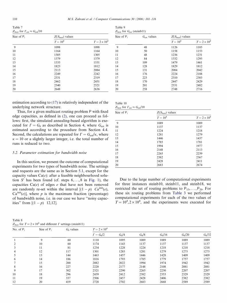
Table 7Zbest for Cest � Gest/10

Size of Pi Z(Sbest) values

T = 104 T = 2 · 104

9 1098 109810 1164 116411 1305 130512 1379 137913 1535 153114 1823 181215 2113 208416 2249 224217 2331 231918 2462 245119 2540 252120 2648 2636

Table 9Zbest for Gest (steinb11)

Size of Pi Gest values Z(Sbest) values

T = 104 T = 2 · 104

9 48 1126 110510 50 1158 115311 48 1236 123112 84 1332 129513 109 1479 146114 128 1829 181215 131 2084 204216 176 2224 218817 223 2310 230318 170 2447 242919 201 2531 248220 258 2748 2716

Table 10Zbest for Cest � Gest/10

Size of Pi Z(Sbest) values

T = 104 T = 2 · 104

9 1089 108910 1137 113711 1224 121812 1281 127913 1446 143714 1785 178115 1994 197716 2148 211317 2265 223918 2382 236719 2428 241120 2683 2674

110 M.S. Zahrani et al. / Computer Communications 30 (2006) 101–116

estimation according to (17) is relatively independent of theunderlying network structure.

Thus, for a given multicast routing problem P with fixededge capacities, as defined in (2), one can proceed as fol-lows: first, the simulated annealing-based algorithm is exe-cuted for C = G0 as described in Section 4, where Gest isestimated according to the procedure from Section 4.4.Second, the calculations are repeated for C = Gest/j, wherej = 10 or a slightly larger integer, i.e. the total number ofruns is reduced to two.

5.2. Parameter estimation for bandwidth noise

In this section, we present the outcome of computationalexperiments for two types of bandwidth noise. The settingsand requests are the same as in Section 5.1, except for thecapacity values Ca(e): after a feasible neighbourhood solu-tion S 0 has been found (cf. steps 6, . . ., 8 in Fig. 1), thecapacities Ca(e) of edges e that have not been removedare randomly re-set within the interval [(1 � p) Æ Cainit(e),Cainit(e)], where p is the maximum fraction (percentage)of bandwidth noise, i.e. in our case we have ‘‘noisy capac-ities’’ from [(1 � p) Æ 12,12].

Table 8Zbest for T = 2 · 104 and different C settings (steinb11)

No. of Pi Size of Pi G0 values T = 2 · 104

C = G0/2

1 9 60 11102 10 60 11743 11 81 12344 12 117 13015 13 144 14636 14 186 18167 15 200 20828 16 227 22209 17 302 2321

10 18 296 243911 19 337 250612 20 419 2728

Due to the large number of computational experimentsfor three instances steinb10, steinb11, and steinb18, werestricted the set of routing problems to P15, . . . ,P20. Forthese six routing problems from Table 3 we performedcomputational experiments for each of the two values ofT = 104,2 · 104, and the experiments were executed for

G0/4 G0/8 G0/16 G0/20 G0/32

1095 1089 1089 1089 10891143 1137 1137 1137 11371228 1224 1218 1218 12181285 1281 1279 1275 12751457 1446 1428 1409 14091793 1785 1779 1757 17572022 1994 1974 1942 19422177 2148 2108 2081 20812290 2265 2230 2207 22072412 2382 2353 2329 23292457 2428 2406 2382 23822702 2683 2668 2589 2589

Table 11Zbest for T = 2 · 104 and different C settings (steinb18)

No. of Pi Size of Pi G0 values T = 2 · 104

C = G0/2 G0/4 G0/8 G0/16 G0/20 G0/32

1 9 64 1365 1341 1335 1335 1335 13352 10 73 1389 1380 1378 1378 1378 13783 11 73 1497 1491 1486 1486 1486 14864 12 134 1628 1618 1606 1594 1594 15945 13 154 1746 1732 1726 1722 1722 17226 14 202 2092 2077 2058 2047 2032 20327 15 223 2273 2252 2236 2218 2204 22048 16 268 2421 2412 2396 2381 2375 23759 17 313 2625 2597 2582 2554 2532 2532

10 18 353 2705 2693 2679 2657 2641 264111 19 397 2807 2797 2765 2749 2735 273512 20 522 3096 3065 3018 2993 2988 2988

Table 12Zbest for Gest (steinb18)

Size of Pi Gest values Z(Sbest) values

T = 104 T = 2 · 104

9 30 1365 134510 42 1389 138311 42 1497 149112 51 1628 161813 87 1756 174314 170 2098 208415 203 2279 226316 206 2423 241417 235 2638 260718 302 2724 269519 329 2817 280220 418 3112 3076

Table 13Zbest for Cest � Gest/10

Size of Pi Zbest values

T = 104 T = 2 · 104

9 1335 133510 1380 137811 1488 148612 1606 159913 1730 172614 2073 205615 2245 223416 2407 238917 2586 256218 2686 267019 2791 275520 3048 3009

M.S. Zahrani et al. / Computer Communications 30 (2006) 101–116 111

six different values of C in (9): C: = G0/c; G0 :¼jZðS1

0Þ�ZðS20Þj.

Two types of bandwidth noise were determined byp = 25% and p = 33%. We first consider p = 25%, and wehave in this case Ca(e) 2 {9,10,11,12} and c = 2,4,8,16,28,36.

As we can see from Tables 14 and 15, the results for Gest

are similar to the results obtained for G0/4, whereas thebest results are produced for G0/36 (Table 16). This obser-vation leads us to the assumption that

Cp¼0:25est � Gp¼0:25

est

9ð18Þ

is an appropriate setting of C in (9) for p = 25%. This isconfirmed by the experiments on steinb11 and steinb18;cf. Tables 17–22.

Again, the results demonstrate that the estimationaccording to (18) is relatively independent of theunderlying network structure.

Finally, we consider the case p = 33%. We haveCa(e) 2 {8,9,10,11,12} and c = 2,4,8,16,28,32. FromTables 23 and 24 we see that the results for Gest are similarto the results obtained for G0/4, and the best results havebeen obtained for G0/32 (Table 25). As in the previoustwo cases we come to the conclusion that

Cp¼0:33est � Gp¼0:33

est

8ð19Þ

can be used as the parameter setting for C in (9) if p = 33%.In Tables 26–31 we present the results for steinb11 and

steinb18. The results confirm the approximation providedin (19) for p = 33%.

In Sections 5.1 and 5.2 we have demonstrated howto apply the landscape analysis introduced in Section4.4 to particular multicast routing problems. We haveseen that with high likelihood a significant differencebetween the monitored value Gest and the landscapeparameter C can be expected. The results suggest thatestimations of type (17)–(19) basically depend on thefunctions Co and Ca rather than on structural proper-ties of the underlying networks. Furthermore, we haveseen how bandwidth noise may affect the relationbetween the approximation of Cest and the observedvalue Gest.

Table 14Zbest for T = 2 · 104 and different C settings (steinb10)

No. of Pi Size of Pi G0 values T = 2 · 104

C = G0/2 G0/4 G0/8 G0/16 G0/28 G0/36

7 15 204 2175 2160 2138 2124 2114 21028 16 248 2325 2316 2305 2289 2274 22569 17 274 2403 2387 2372 2359 2344 2330

10 18 297 2524 2513 2502 2490 2476 246811 19 345 2627 2608 2595 2579 2563 254212 20 402 2731 2715 2701 2684 2672 2658

Table 15Zbest for Gest (steinb10)

Size of Pi Gest values Z(Sbest) values

T = 104 T = 2 · 104

15 126 2182 215716 153 2325 231617 177 2405 238718 186 2527 251619 214 2630 260820 231 2733 2718

Table 18Zbest for Gest (steinb11)

Size of Pi Gest values Z(Sbest) values

T = 104 T = 2 · 104

15 205 2088 206916 221 2233 220717 244 2399 237518 268 2507 248619 317 2534 251120 332 2802 2781

Table 16Zbest for Cest � Gest/9

Size of Pi Z(Sbest) values

T = 104 T = 2 · 104

15 2160 213316 2312 230217 2381 236518 2513 249719 2605 259020 2713 2698

Table 19Zbest for Cest � Gest/9

Size of Pi Z(Sbest) values

T = 104 T = 2 · 104

15 2071 205316 2207 218417 2370 233918 2485 246019 2506 248720 2778 2766

112 M.S. Zahrani et al. / Computer Communications 30 (2006) 101–116

5.3. Comparison to GA with PMX crossover

For comparison purposes, we have implemented thegenetic algorithm described in Section 3, which is basedon the PMX crossover operation [15,47]. The implementa-tion has been applied to P15, . . . ,P20 from Table 3 for thecase of fixed capacities (no bandwidth noise). Here, wereport the results for steinb18 only.

The population size M was chosen equal to 10, and thenumber NPMX of applications of PMX crossover

Table 17Zbest for T = 2 · 104 and different C settings (steinb11)

No. of Pi Size of Pi G0 values T = 2 · 104

C = G0/2

7 15 327 20838 16 348 22279 17 383 2392

10 18 423 249811 19 461 252312 20 489 2797

operations equal to 2 · 103, i.e. the product is equal tothe number of transitions T = 2 · 104, which wasconsidered in Section 5.1 for logarithmic simulated anneal-ing. The selection process after PMX operations was exe-cuted under the elitist model.

In Table 32, the results for LSA are taken from Table 11(best LSA) and Table 13 for Cest � Gest/10. On all instancesP15, . . . ,P20, the simulated annealing procedure, which isbased on inhomogeneous Markov chains, achieves betterresults than the genetic algorithm with PMX crossover.

G0/4 G0/8 G0/16 G0/28 G0/36

2071 2061 2048 2031 20082209 2190 2178 2171 21342373 2359 2334 2317 22952486 2472 2455 2446 24212511 2494 2478 2451 24392781 2771 2751 2744 2720

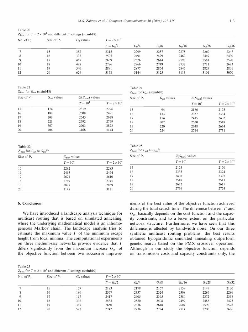
Table 24Zbest for Gest (steinb10)

Size of Pi Gest values Z(Sbest) values

T = 104 T = 2 · 104

15 94 2186 217516 133 2357 233417 154 2415 240218 207 2530 251819 220 2648 263420 224 2744 2731

Table 20Zbest for T = 2 · 104 and different C settings (steinb18)

No. of Pi Size of Pi G0 values T = 2 · 104

C = G0/2 G0/4 G0/8 G0/16 G0/28 G0/36

7 15 352 2315 2299 2287 2275 2260 22478 16 393 2505 2491 2479 2462 2449 24309 17 467 2639 2626 2614 2598 2581 2570

10 18 498 2786 2766 2749 2732 2711 268311 19 540 2891 2877 2864 2845 2829 280112 20 626 3158 3144 3125 3113 3101 3070

Table 25Zbest for Cest � Gest/8

Size of Pi Z(Sbest) values

T = 104 T = 2 · 104

15 2175 217016 2335 232417 2408 239518 2518 251119 2632 261520 2736 2724

Table 21Zbest for Gest (steinb18)

Size of Pi Gest values Z(Sbest) values

T = 104 T = 2 · 104

15 174 2319 229616 189 2508 249117 208 2645 262818 221 2792 276919 367 2903 287320 406 3168 3144

Table 22Zbest for Cest � Gest/9

Size of Pi Zbest values

T = 104 T = 2 · 104

15 2292 228316 2493 247417 2621 261018 2769 274519 2877 285920 3148 3121

M.S. Zahrani et al. / Computer Communications 30 (2006) 101–116 113

6. Conclusion

We have introduced a landscape analysis technique formulticast routing that is based on simulated annealing,where the underlying mathematical model is an inhomo-geneous Markov chain. The landscape analysis tries toestimate the maximum value C of the minimum escapeheight from local minima. The computational experimentson three medium-size networks provide evidence that Cdiffers significantly from the maximum increase Gest ofthe objective function between two successive improve-

Table 23Zbest for T = 2 · 104 and different C settings (steinb10)

No. of Pi Size of Pi G0 values T = 2 · 104

C = G0/2

7 15 159 21838 16 180 23579 17 197 2417

10 18 306 253511 19 367 265012 20 523 2742

ments of the best value of the objective function achievedduring the total search time. The difference between C andGest basically depends on the cost function and the capac-ity constraints, and to a lesser extent on the particularnetwork structure. Furthermore, we have seen that thisdifference is affected by bandwidth noise. On our threesynthetic multicast routing problems, the best resultsobtained bylogarithmic simulated annealing outperformgenetic search based on the PMX crossover operation.Although in our study the objective function dependson transmission costs and capacity constraints only, the

G0/4 G0/8 G0/16 G0/28 G0/32

2178 2167 2159 2147 21302337 2324 2308 2295 22862405 2395 2380 2372 23582520 2508 2499 2488 24732636 2618 2604 2590 25782736 2724 2714 2700 2686

Table 26Zbest for T = 2 · 104 and different C settings (steinb11)

No. of Pi Size of Pi G0 values T = 2 · 104

C = G0/2 G0/4 G0/8 G0/16 G0/28 G0/32

7 15 348 2088 2078 2069 2050 2035 20178 16 380 2286 2267 2237 2222 2209 22019 17 422 2415 2394 2387 2380 2375 2346

10 18 309 2574 2553 2541 2531 2502 246311 19 470 2671 2634 2612 2581 2555 253512 20 511 2954 2912 2880 2862 2818 2809

Table 27Zbest for Gest (steinb11)

Size of Pi Gest values Z(Sbest) values

T = 104 T = 2 · 104

15 288 2088 207816 270 2276 226817 317 2406 239418 232 2567 255019 347 2650 263420 376 2949 2905

Table 30Zbest for Gest (steinb18)

Size of Pi Gest values Z(Sbest) values

T = 104 T = 2 · 104

15 160 2327 231516 225 2558 254117 215 2701 269018 223 2880 285819 381 2996 298420 417 3221 3215

Table 32Zbest for LSA and elitist PMX (steinb18)

Size of Pi T = 2 · 104 M = 10 and NPMX = 2 · 103

Cest � Gest/10 Best LSA Elitist PMX

15 2234 2204 221816 2389 2375 238517 2562 2532 253918 2670 2641 2653

Table 28Zbest for Cest � Gest/8

Size of Pi Z(Sbest) values

T = 104 T = 2 · 104

15 2078 206916 2254 223917 2394 238718 2553 254119 2629 261520 2892 2880

Table 31Zbest for Cest � Gest/8

Size of Pi Zbest values

T = 104 T = 2 · 104

15 2302 229816 2533 253017 2690 268818 2847 284119 2970 295820 3213 3209

114 M.S. Zahrani et al. / Computer Communications 30 (2006) 101–116

approach is applicable to more complex objective func-tions that take into account various QoS requirements.Future research will be directed towards a deeper analysisof the structure of energy landscapes induced by multicastrouting problems.

Table 29Zbest for T = 2 · 104 and different C settings (steinb18)

No. of Pi Size of Pi G0 values T = 2 · 104

C = G0/2 G0/4 G0/8 G0/16 G0/28 G0/32

7 15 242 2327 2312 2298 2286 2281 22698 16 324 2554 2539 2527 2515 2504 24879 17 377 2698 2692 2685 2660 2641 2616

10 18 313 2875 2858 2841 2832 2812 279211 19 511 2995 2977 2968 2952 2940 291612 20 570 3223 3215 3209 3195 3180 3158

19 2755 2735 274920 3009 2988 2993

M.S. Zahrani et al. / Computer Communications 30 (2006) 101–116 115

Acknowledgement

The author thank the anonymous referees for their care-ful reading of the manuscript and many helpful suggestionsthat resulted in an improved presentation.

References

[1] V.B. Muchnik, A.V. Shafarenko, Dynamic evaluation strategy forfine-grain data-parallel computing, IEE Proceedings – Computers andDigital Techniques 143 (3) (1996) 181–188.

[2] H. Abdel-Wahab, K. Maly, E. Stoica, A. Youssef, The role ofmulticasting in managing interactive multimedia distance learningsystems, Journal of Network and Systems Management 5 (3) (1997)351–367.

[3] C. Diot, W. Dabbous, J. Crowcroft, Multipoint communication: asurvey of protocols, functions, and mechanisms, IEEE Journal onSelected Areas in Communications 15 (3) (1997) 277–290.

[4] E. Al-Shaer, Y. Tang, QoS path monitoring for multicast networks,Journal of Network and Systems Management 10 (3) (2002) 357–381.

[5] P. Rajvaidya, K.N. Ramachandran, K.C. Almeroth, Managing andsecuring the global multicast infrastructure, Journal of Network andSystems Management 12 (3) (2004) 297–326.

[6] C.K. Yeo, B.S. Lee, M.H. Er, A survey of application level multicasttechniques, Computer Communications 27 (2004) 1547–1568.

[7] X. Li, B. Veeravalli, Design and performance analysis of multimediadocument retrieval strategies for networked Video-on-Reservationsystems, Computer Communications 28 (2005) 1910–1924.

[8] X. Masip-Bruin, M. Yannuzzi, J. Domingo-Pascual, A. Fonte, M.Curado, E. Monteiro, F. Kuipers, P. Van Mieghem, S. Avallone, G.Ventre, P. Aranda-Gutierrez, M. Hollick, R. Steinmetz, L. Iannone,K. Salamatian, Research challenges in QoS routing, ComputerCommunications 29 (2006) 563–581.

[9] T. Harrison, C. Williamson, A performance study of multicastrouting algorithms for ATM networks, in: Proc. 21st Annual IEEEConference on Local Computer Networks, 1996, p. 191.

[10] N. Mir-Fakhraei, An efficient multicast approach in an ATMswitching Network for multimedia applications, Journal of Networkand Computer Applications 21 (1998) 31–39.

[11] W. Jia, G. Xu, W. Zhao, P.O. Au, Efficient internet multicast routingusing anycast path selection, Journal of Network and SystemsManagement 10 (4) (2002) 417–438.

[12] C.K. Yeo, B.S. Lee, M.H. Er, A framework for multicast videostreaming over IP networks, Journal of Network and ComputerApplications 26 (2003) 273–289.

[13] R.M. Karp, Reducibility among combinatorial problems, in: R.E.Miller, J.W. Thatcher (Eds.), Complexity of Computer Computa-tions, Plenum Press, New York, 1972, pp. 85–103.

[14] M. Doar, I.M. Leslie, How bad is naıve multicast routing?, in: Proc.INFOCOM, 1993, pp. 82–89.

[15] L. Zhu, R.L. Wainwright, D.A. Schoenefeld, A genetic algorithm forthe point to multipoint routing problem with varying number ofrequests, in: Proc. IEEE International Conference on EvolutionaryComputation, 1998, pp. 171–176.

[16] Y. Leung, G. Li, Z.B. Xu, A genetic algorithm for the multipledestination routing problems, IEEE Transactions on EvolutionaryComputation 2 (4) (1998) 150–161.

[17] P. Galiasso, R.L. Wainwright, A hybrid genetic algorithm for thepoint to multipoint routing problem with single split paths, in: Proc.ACM Symposium on Applied Computing, 2001, pp. 327–332.

[18] H. Wang, J. Fang, Y.-M. Sun, TSDLMRA: An efficient multicastrouting algorithm based on tabu search, Journal of Network andComputer Applications 27 (2) (2004) 77–90.

[19] C.B. Yang, U.P. Wen, Applying tabu search to backup path planningfor multicast networks, Computers and Operations Research 32(2005) 2875–2889.

[20] S. Kirkpatrick, C.D. Gelatt Jr., M.P. Vecchi, Optimization bysimulated annealing, Science 220 (1983) 671–680.

[21] V. Cerny, A thermodynamical approach to the travelling salesmanproblem: an efficient simulation algorithm, Journal of OptimizationTheory and Applications 45 (1985) 41–51.

[22] B. Hajek, Cooling schedules for optimal annealing, Mathematics ofOperations Research 13 (1988) 311–329.

[23] O. Catoni, Rough large deviation estimates for simulated annealing:applications to exponential schedules, Annals of Probability 20 (1992)1109–1146.

[24] E.H.L. Aarts, Local Search in Combinatorial Optimization, Wiley &Sons, New York, 1998.

[25] Y. Cui, K. Xu, J.P. Wu, Z.C. Yu, Y.J. Zhao, Multi-constrainedrouting based on simulated annealing, in: Proc. IEEE Int. Conf. onCommunications, 2003, vol. 3, pp. 1718–1722.

[26] X.W. Wang, H. Cheng, J. Cao, L.W. Zheng, M. Huang, A simulated-annealing-based QoS multicasting algorithm, in: Proc. Int. Conf. onCommunication Technology, 2003, pp. 469–473.

[27] X.L. Wang, Z. Jiang, QoS multicast routing based on simulatedannealing algorithm, in: S.J.B. Yoo, K.W. Cheung, Y.C. Chung, G.C.Li (Eds.), Proc. SPIE on Network Architectures, Management, andApplications, 2004, pp. 511–516.

[28] Z. Kun, W. Heng, L. Feng-Yu, Distributed multicast routing fordelay and delay variation-bounded Steiner tree using simulatedannealing, Computer Communications 28 (2005) 1356–1370.

[29] S. Banerjee, C. Kommareddy, K. Kar, B. Bhattacharjee, S. Khulle,OMNI: an efficient overlay multicast infrastructure for real-timeapplications, Computer Networks 50 (6) (2006) 826–841.

[30] X. Wang, J. Cao, H. Cheng, M. Huang, QoS multicast routingfor multimedia group communications using intelligent computa-tional methods, Computer Communications 29 (12) (2006) 2217–2229.

[31] S. Wright, The roles of mutation, inbreeding, crossbreeding andselection in evolution, in: Proc. Sixth Int. Congress on Genetics, 1932,vol. 1, pp. 356–366.

[32] P. Merz, B. Freisleben, Fitness landscapes, memetic algorithms, andgreedy operators for graph bipartitioning, Evolutionary Computation8 (1) (2000) 61–91.

[33] Ch.M. Reidys, P.F. Stadler, Combinatorial landscapes, SIAMReview 44 (1) (2002) 3–54.

[34] D. Wales, Energy Landscapes, Cambridge University Press, Cam-bridge, 2003.

[35] A.A. Albrecht, A stopping criterion for logarithmic simulatedannealing, Computing 78 (1) (2006) 55–79.

[36] F.F. Ferreira, J.F. Fontanari, P.F. Stadler, Landscape statistics of thelow-autocorrelation binary string problem, Journal of Physics A-Mathematical and General 33 (2000) 8635–8647.

[37] M.T. Wolfinger, W.A. Svrcek-Seiler, Ch. Flamm, I.L. Hofacker, P.F.Stadler, Exact folding dynamics of RNA secondary structures,Journal of Physics A-Mathematical and General 37 (2004) 4731–4741.

[38] L.M. Schmitt, Theory of genetic algorithms, Theoretical ComputerScience 259 (2001) 1–61.

[39] M.S. Zahrani, M.J. Loomes, J.A. Malcolm, A.A. Albrecht, Geneticlocal search for multicast routing, in: Proc. 8th Annual Conference onGenetic and Evolutionary Computation (GECCO’06), ACM Press,New York, 2006, pp. 615–616.

[40] K. Steinhofel, A. Albrecht, C.K. Wong, Fast parallel heuristics forthe job shop scheduling problem, Computers and OperationsResearch 29 (2) (2002) 151–169.

[41] J.E. Beasley, OR-library: <http://people.brunel.ac.uk/~mastjjb/jeb/info.html/>.

[42] S.L. Hakimi, Steiner’s problem in graphs and its implications,Networks 1 (1971) 113–133.

[43] L. Kou, G. Markowsky, L. Berman, A fast algorithm for Steinertrees, Acta Informatica 15 (1981) 141–145.

[44] M.J. Alexander, G. Robins, New performance-driven FPGA routingalgorithm, in: Proc. ACM/SIGDA Design Automation Conference,1995, pp. 562–567.

116 M.S. Zahrani et al. / Computer Communications 30 (2006) 101–116

[45] T. Koch, A. Martin, Solving Steiner tree problems in graphs tooptimality, Networks 32 (1998) 207–232.

[46] H.-J. Promel, A. Steger, A new approximation algorithm for theSteiner tree problem with performance ratio 5/3, Journal ofAlgorithms 36 (2000) 89–101.

[47] P. Baudet, C. Azzaro, L. Pibouleau, S. Domenech, A geneticalgorithm for batch chemical plant scheduling, in: Proc. Int. Congressof Chemical and Process Engineering, 1996, pp. 25–30.

Mohammed S. Zahrani received his MSc degreein Computer Science in 2002 from WesternMichigan University. In 2003, he worked as aLecturer at King Faisal University, Saudi Arabia.Afterwards, he joined the School of ComputerScience Department at the University of Hert-fordshire, where he is pursuing his PhD in thearea of computer and communications networks.

Martin J. Loomes is Dean of Computing Scienceat Middlesex University, UK. He received hisPhD from the Department of Electrical andElectronic Engineering at the University of Sur-rey, and is a Chartered Mathematician and Sci-entist. He spent sixteen years managingComputer Science research at the University ofHertfordshire, prior to his recent move to Mid-dlesex in 2005. His areas of research interest havealways focused on the interfaces between math-ematics, computing and psychology, which has

led naturally to several projects in the area of machine learning withapplications as diverse as face recognition, identifying wake-vortex

encounters and routing algorithms.

James A. Malcolm has an MA from the Univer-sity of Cambridge, awarded in 1976, having pre-viously gained a BA in Natural Sciences and aDiploma in Computer Science. He worked as aprogrammer at Rothamsted Experimental Sta-tion and at GEC Computers Ltd., before joiningUniversity College London where he becameteam leader on the Alvey funded ADMIRALproject. Since 1988 he is with the School ofComputer Science at the University of Hert-fordshire. His areas of interest and expertise

include computer networks, Internet technology and applications, com-puter security and the prevention and detection of student plagiarism.

Andreas A. Albrecht is a Senior Lecturer in theSchool of Computer Science at HertfordshireUniversity. He received the Diploma in AppliedMathematics (BSc plus MSc equivalent) fromMoscow State University, and the PhD (Dr.rer.nat.) and the Habilitation (Dr.sc.nat.) degrees inComputational Mathematics from HumboldtUniversity at Berlin. His research interestsinclude Combinatorial Optimization, CircuitComplexity, Bioinformatics, and MachineLearning.