A Stability-based Distributed Routing Mechanism to Support Unicast and Multicast Routing

in Ad Hoc Wireless Network

Krishna Paul #, S. Bandyopadhyay*, A. Mukherjee * , D. Saha +

Abstract An ad hoc network can be envisioned as a collection of mobile routers, each equipped with a

wireless transceiver, which are free to move about arbitrarily. In ad hoc wireless networks,

even if two nodes are outside the wireless transmission range of each other, they may still be

able to communicate in multiple hops using other intermediate nodes. However, the dynamics

of these networks, as a consequence of mobility and disconnection of mobile hosts, pose a

number of problems in designing routing schemes for effective communication between any

pair of source and destination. In this paper, a stability-based unicast routing mechanism, that

considers both link affinity and path stability in order to find out a stable route from source to

destination, is proposed. It is then extended to support multicast routing as well where only

local state information (at source) is utilized for constructing a multicast tree. The

performance of the proposed scheme is evaluated on a simulated environment to show that the

stability-based scheme provides a unified framework for both unicast and multicast routing

and reduces the probability of route error drastically in both the cases.

--------------------------------------------------------------------------------------------------------------------------------- # Cognizant Technology Solutions, Sector V, Calcutta 700 091, India. E-mail: pkrishna2@cal.cts-corp.com * PricewaterhouseCoopers Ltd., Sector V, Saltlake, Calcutta 700 091India. E-mail: {amitava.mukherjee, Somprakash.Bandyopadhyay}@in.pwcglobal.com + Department of Computer Science, Jadavpur University, Calcutta 700 032, India. E-mail: d.saha@vsnl.com

1

1. Introduction Ad hoc wireless networks are self-organizing network architectures of mobile nodes that are

rapidly deployable and that adapt to the propagation conditions and to the traffic and mobility

patterns of the network nodes [1]. An ad hoc network can be envisioned as a collection of

mobile routers, each equipped with a wireless transceiver, which are free to move about

arbitrarily. The mobility of the routers and the variability of other connecting factors result in

a network with a potentially rapid and unpredictable changing topology. These networks may

or may not be connected with the infrastructure such as internet, but still be available for use

by a group of wireless mobile hosts that operate without any base-station or any centralized

control. Applications of ad hoc networks include military tactical communication, emergency

relief operations, commercial and educational use in remote areas, where the networking is

mission-oriented and / or community-based.

There has been a growing interest in ad hoc networks in recent years [2,3,4,5,6,7]. The

basic assumption in an ad hoc network is that two nodes willing to communicate may be

outside the wireless transmission range of each other but still be able to communicate if other

nodes in the network are willing and capable of forwarding packets from them. However, the

successful operation of an ad-hoc network will be hampered, if an intermediate node,

participating in a communication between two nodes, either moves out of range suddenly or

switches itself off in between message transfer. The situation is worse, if there is no

alternative path available between those two nodes.

In general, existing routing protocols can be classified either as proactive or as reactive

[1]. In proactive protocols, the routing information within the network is always known

beforehand through continuous route updates. The distance vector and link state protocols are

examples of proactive scheme. Examples of proactive routing methods in ad hoc network

environments are given in [8,9]. However, these methods require to know the topology of the

entire network and this information needs to be propagated through the network.

Consequently, in a highly dynamic environment, these schemes are less efficient.

Reactive protocols, on the other hand, invoke the route discovery procedure on demand

only. The family of classical flooding algorithms belongs to this group. Examples of reactive

protocols in the context of ad hoc networks can be found in [2,3,4,5,6]. It has been pointed out

that proactive protocols are not suitable for highly mobile ad hoc network, since they consume

2

a large portion of network capacity for continuously updating route information [10]. On the

other hand, on-demand search procedure in reactive protocols generate large volume of

control traffic and the actual data transmission is delayed until the route is determined. The

features, problems and requirements associated with different routing schemes in ad-hoc

network are illustrated in [11, 12,13,14] through qualitative and simulation studies.

Whatever may be the routing scheme, frequent interruption in a selected route would

degrade the performance in terms of quality of service. Therefore, an important issue is to

minimize route maintenance by selecting stable routes, rather than shortest routes. In an ad

hoc network, relationship among nodes is based on providing some kind of service, and

stability can be defined as the minimal interruption in that service. Hence, a notion of stability

of a path and its evaluation mechanism in the context of dynamic topology changes in an ad-

hoc network is introduced in this work and a distributed routing scheme among mobile hosts

is proposed in order to find a path between them which is stable in a specific context.

The idea of selecting stable routes within a dynamic network has been proposed in [5,6].

In Associativity Based Routing [5], an optimal route is selected based on the stability of the

route. The notion of stability of an intermediate node is based on a Rule of Associativity that

states that a node’s association with its neighbor changes as it migrates from one wireless cell

to another. This migration is such that, after this unstable period, there exists a period of

stability, where the node will spend some dormant time within a wireless cell before its starts

to move again. In Signal-Stability based Adaptive Routing [6], stable routes are selected

based on signal strength. The signal strength criteria allows the protocol to differentiate

between strong channels and weak channels. Each channel is characterized by the average

signal strength at which packets are exchanged between the nodes at either end of the channel.

The routes with strong channels are likely to be long-lived (i.e. stable). However, a major

drawback of these methods is that the parameter stability is not explicitly evaluated.

Moreover, the notion of stability of a path is dynamic and context-sensitive. Stability of a path

is the span of life of that path at a given instant of time and it has to be seen in the context of

providing a service. A path between a source and a destination would be stable if its span of

life is sufficient to complete a required volume of data transfer from source to destination

without possible interruption. Hence, a given path may be sufficiently stable to transfer a

3

small volume of data between source and destination; but the same path may be unstable in a

context where a large volume of data needs to be transferred.

This work first proposes a stability-based unicast routing mechanism and then extends it

to a multicast routing mechanism that depends only on local state information (at source) for

constructing a multicast tree. Multicast communication in the context of ad hoc wireless

network is a very useful and efficient means of supporting group-oriented applications, where

the need for one-to-many data dissemination is quite frequent in critical situations such as

disaster recovery or battlefield scenarios. Instead of sending data via multiple unicasts,

multicast routing reduces the communication costs by minimizing the link bandwidth

consumption and delivery delay.

Research in the area of routing in ad-hoc wireless network has mostly concentrated on

designing effective routing schemes for unicast communication. Those routing algorithms

were not designed with multicast extensions in mind. Therefore, they do not naturally support

multicast routing solutions [15]. Since fixed network multicasting is based on state in routers

(either hard or soft), it is fundamentally unsuitable for ad hoc network where topology is

changing frequently due to unconstrained mobility. It has been shown that the performance of

both hard- and soft-state multicast tree maintenance mechanisms degrade rapidly with

increased mobility [16]. Traditional multicast approaches that rely on maintaining and

exchanging multicast-related state information are not suitable in highly dynamic ad-hoc

network with frequent and unpredictable changing topology [15].

Currently proposed ad hoc multicast routing schemes [16] lie on a spectrum that spans

from pure Internet multicast routing based schemes to a pure flooding scheme. Internet

multicast routing schemes, as it is currently, generally require the routing nodes to maintain

fairly large amount of state information for routing and to use processing power of hosts

rather liberally. Feasibility of supporting continuous unlimited mobility is also a question with

Internet routing schemes. Only flooding control packets may support unlimited continuous

mobility. Flooding will also reduce the amount of state information kept at mobile hosts, and

will provide reliable and timely delivery.

FGMP [17], the Forwarding Group Multicast Protocol, proposes a scheme that is hybrid

between flooding and source based tree multicast. The proposed multicast protocol scheme

keeps track not of links but of groups of nodes which participate in multicast packets

4

forwarding. To each multicast group G is associated a forwarding group, FG. Any node in FG

is in charge of forwarding (broadcast) multicast packets of G. The nodes to be included in FG

are elected according to members’ requests. Instead of data packets, small membership

advertisement packets are used to reduce overhead caused by broadcasting. However, in order

to advertise the membership, each receiver periodically and globally flood its member

information.

AMRoute [18], the Ad hoc Multicast Routing Protocol, creates a per group multicast

distribution tree using unicast tunnels connecting group members. The protocol has two main

components: mesh creation and tree creation. Certain nodes are designated as logical core

nodes that initiate mesh and tree creation; however, the core can migrate dynamically

according to group membership and network connectivity. Logical cores are responsible for

initiating and managing the signaling component of AMRoute, such as detection of group

members and tree set up. Bi-directional tunnels are created between pairs of group members

that are close together, thus forming a mesh. Using a subset of available mesh links, the

protocol periodically creates a multicast distribution tree. AmRoute assumes the existence of

an underlying unicast routing protocol and its performance is influenced by the characteristics

of the unicast routing protocol being used. The AMRoute simulation runs on top of TORA [5]

as underlying unicast protocol. The network dynamicity was emulated by keeping node

location fixed and breaking / connecting links between neighboring nodes. Thus, the effect of

actual node mobility on the performance is difficult to interpret. Moreover, the signaling

generated by underlying unicast protocol (TORA in this case) is not considered in the

measurements.

The Core- Assisted Mesh Protocol (CAMP) [19] generalizes the notion of core-based

trees introduced for internet multicasting into multicast meshes that have much richer

connectivity than trees. A shared multicast mesh is defined for each multicast group. The

advantage of using such meshes is to maintain the connectivity even while the network

routers move frequently. CAMP consists of the maintenance of multicast meshes and loop-

free packet forwarding over such meshes. Multicast packets for a group are forwarded along

the shortest path from sources to receivers defined within the group’s mesh. CAMP rebuilds

meshes at least as fast as CBT and PIM can rebuild trees. However, the effect of mobility on

the performance has not been clearly evaluated. The topology under experimentation has 30

5

routers with high connectivity ( average of six neighbors each) and at the most 15 routers out

of 30 are assumed to be mobile.

AMRIS [20], the Adhoc Multicast Routing Protocol utilizing Increasing id-numberS,

assigns an identifier to each node in a multicast session. A pre-multicast session delivery tree

rooted at a special node (by necessity a sender) in the session joins all the group members.

The tree structure is maintained by assigning identifiers in increasing order from the tree root

outward to the other group members. All nodes are required to process the tree set up and

maintenance messages that are transmitted by the root periodically. It has been assumed that

most multicast applications are long-lived; therefore rapid route reconstruction is of greater

importance compared to rapid route discovery. The performance of the proposed scheme has

yet to be evaluated.

ODMRP [21], the On-Demand Multicast Routing Protocol, also uses a mesh-based

approach for data delivery and uses a forwarding group concept. It requires sources rather

than destinations to initiate the mesh building by periodic flooding of control packets. It

applies on-demand procedures to dynamically build routes and maintain multicast group

membership. A soft-state approach is taken to maintain multicast group member.

This paper proposes a multicast routing mechanism that depends only on local state

information (at source) for constructing a multicast tree. It is demand- driven in the sense that

whenever a source needs to communicate with a set of destinations, it discovers the routes and

creates a multicast tree dynamically. It has been shown that the proposed multicast routing

scheme reduces both the control traffic and the data traffic and decreases the delivery delay

considerably when compared to multiple unicasts.

2 Description of the Proposed Framework 2.1 System Description

The network is modeled as a graph G = (N,L) where N is a finite set of nodes distributed over

a two-dimensional space of area A and L is a finite set of unidirectional links. Each node n ∈

N is having a unique node identifier. In a wireless environment, each node n has a wireless

transmitter range Rn . If a node m is within the transmission range of n, then n and m are assumed to be

connected by a unidirectional links lnm ∈L, such that whenever n broadcasts a message, it will be

received by m via lnm. Similarly, if n is within the transmission range of m, then m and n are assumed

6

to be connected by a unidirectional links lmn ∈ L, such that whenever m broadcasts a message, it will

be received by n via lmn. Since in a wireless environment, transmission between two nodes n and

m does not necessarily work equally well in both directions and Rn may not be equal to Rm,

lnm and lmn may be unequal.

Each link lnm is associated with a signal-strength Snm which is a measurable indicator of

the strength of connection from n to m as perceived by m at any instant of time. Due to the

mobility of nodes, signal strengths associated with the links changes with time. When the

signal strength Snm associated with lnm goes below a certain threshold St, we assume that the

link lnm is disconnected.

We define the neighbors of n, Nn∈N, to be the set of nodes within the transmission range

of n. It is assumed that when node n transmits a packet, the packet is broadcast to all of its

neighbors in the set Nn. However, in the wireless environment, the strength of connection of

all the members of Nn with respect to n are not equal. For example, a node m∈Nn, which is in

the periphery of the transmission range of n, is weakly connected to n compared to a node

p∈Nn which is more closer to n. Thus, the chance of m going out of the transmission range of

n (due to an outward mobility of either m or n) is more than that of p.

We define the strength of relationship between two nodes over a period of time as node-

affinity or affinity. Informally speaking, link-affinity anm(t), associated with a link lnm at time

t, is a prediction about the span of life of the link lnm in a particular context. Link-affinity

anm(t) at that instant of time is a function of the current distance between n and m, relative

mobility of m with respect to n, and the transmission range of n. If transmission range of n

and m are different, anm(t) may not be equal to amn(t). The node-affinity or affinity ηnm(t)

between two nodes n and its neighbor m is defined as min[anm(t), amn(t)]. The stability of

connectivity between n and its neighbor m depends on ηnm(t). The unit of affinity is seconds.

2.2 Predicting Affinity between Nodes

To find out the link-affinity anm(t) at any instant of time, node n sends a periodic beacon and

node m samples the strength of signals received from node n periodically. Since the signal

strength of n as perceived by m is a function f(Rn, dnm) where Rn is the transmission range of n, and dnm

is the current distance between n and m at time t, the node m can predict the current distance dnm at

7

time t between n and m. If M is the average velocity of the nodes, the worst-case link-affinity anm(t) at

time t is (Rn-dnm)/M, assuming that at time t, the node m has started moving outwards with an average

velocity M. For example, If the transmission range of n is 300 meters, the average velocity is 10m/sec

and current distance between n and m is 100 meters, the life-span of link lnm (worst-case) is 20

seconds, assuming that the node m is moving away from n in a direction obtained by joining n and m.

The above method is simple, but is based on an optimistic assumption that node-distance

can be deduced from signal strength. In real life, even if the transceivers have the same

transmission range, it will vary because of the differences in battery power in each of them.

Therefore, it may be difficult for one node to estimate distance from another node by

monitoring the current signal strength only. So, a node m needs to monitor the change in

signal strength of n over time to estimate link-affinity, as described below.

Let ∆Snm(t) be the change of signal strength at time t and is defined as:

∆Snm(t) = Snm(t) – Snm(t- ∆t), where Snm(t) is the current sample value of the signal strength of

node n as perceived by node m at time t, Snm(t- ∆t) is the previous sample value at time (t- ∆t)

and ∆t is the sampling interval. Let S′nm(t) be the rate of change of signal strength at time t

and is defined as S′nm(t) = (∆Snm(t) / ∆t ) and let S′nm(t)avg is the average rate of change of

signal strength at time t over the past few samples. Let St be the threshold-signal-strength :

when the signal strength Snm associated with lnm goes below St, we assume that the link lnm is

disconnected. Further we define

anm (t) = high, if S′nm(t)avg is positive;

= (St - Snm(t) ) / S′nm(t)avg, if S′nm(t)avg is negative.

If ∆Snm(ave) is positive, it indicates that the link-affinity is increasing and the two nodes are

coming closer. Hence, link-affinity is termed as high at that instant of time. The value for

high is computed as (transmission range / average node velocity) and is approximately equal

to the time taken by a node m to cross the average transmission range of node n with an

average velocity. However, as indicated earlier, even if S′nm(t)avg is positive, a node m∈Nn in

the periphery of the transmission range of n is weakly connected to n compared to a node

p∈Nn which is closer to n. Thus, the chance of m going out of the transmission range of n

due to a sudden outward mobility of either m or n is more than that of p. Thus, if S′nm(t)avg is

positive, a correction factor µ is used to moderate this high value. This correction factor µ is

8

equal to (1 - St / Snm(t)) and anm(t) = µ* high, if S′nm(t)avg is positive. This indicates that if

Snm(t) is very close to St, µ will be close to zero and consequently anm(t) will also become

close to zero, even if S′nm(t)avg is positive.

As indicated earlier, the node-affinity or affinity between two nodes n and m, ηnm(t), is

defined as min[anm(t) , amn(t)].

2.3 Stability of a path Given any path p = (i, j, k, …, l, m), the stability of path p will be determined by the lowest-

affinity link (since that is the bottleneck for the path) and is defined as :

min[ηij(t), ηjk(t), …, ηlm(t)]. In other words, stability of path p at some instant of time t

between source s and destination d, ηpsd(t), is given by: ηp

sd(t) = min [ηij(t)], ∀i,j ∈ p.

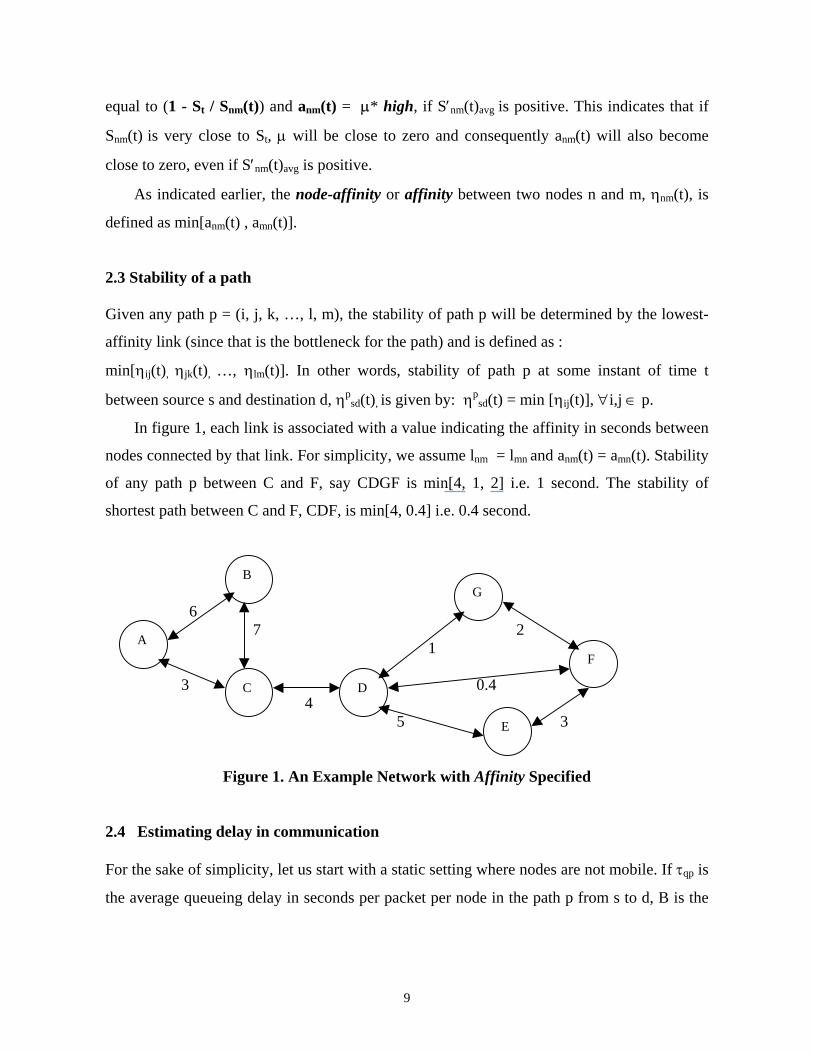
In figure 1, each link is associated with a value indicating the affinity in seconds between

nodes connected by that link. For simplicity, we assume lnm = lmn and anm(t) = amn(t). Stability

of any path p between C and F, say CDGF is min[4, 1, 2] i.e. 1 second. The stability of

shortest path between C and F, CDF, is min[4, 0.4] i.e. 0.4 second.

6 7 2 A 1 3 0.4 4 5 3

C

G

F

E

B

D

A

Figure 1. An Example Network with Affinity Specified 2.4 Estimating delay in communication

For the sake of simplicity, let us start with a static setting where nodes are not mobile. If τqp is

the average queueing delay in seconds per packet per node in the path p from s to d, B is the

9

bandwidth in packets per second and tp is the average delay in seconds per hop per packet of a

traffic stream on the path p, then

tp = τqp + 1/B , ignoring processing delay.

The first component is the queuing delay and the second component is the delay due to packet

transmission time.

If Tp is the total average packet delay for the path p from s to d with number of hops Hp , then

Tp = Hp * tp

DCBA S

Figure 2. Data Communication from Source S to Destination D

Consider the situation shown in figure 2 where S is sending data to D which is 4-hops away

from S in a collision-free environment. When S is transmitting a data packet. A has to be in

receive mode to accept the packet; B also can not be in transmit mode to avoid interference

with A’s reception. However, C can transmit simultaneously to D, if C has any data packet to

send. Thus, there is a chance of establishing a pipelined transmission, if number of hops is

more than 3. However, there is also a chance that S will complete its entire data transfer

activity to A before A gets a chance to transmit. So, the worst case end-to-end delay per

packet is Hp * tp.

Now, let us consider a dynamic scenario where nodes are mobile. It implies that an

intermediate node in path p, participating in a communication between two nodes s and d,

may move out of transmission range suddenly or may switch itself off in between message

transfer. In other words, path p between s and d may not be stable enough to complete the

desired communication and we may need to rediscover another path p to complete the data

transfer. In that case, the remaining packets need to be transmitted from s to d over the new

path. If V is the number of packets to be transmitted from s to d, tpRD is the route discovery

time for path p from s to d, ν is the number of times route rediscovery required for completing

data transfer from s to d and Td is the time taken by the source to detect the occurrence of a

route error, then the total delay for the path p from s and d is given by :

10

Total_Delaysd = ∑Vk=1Tp

k + ∑p=1ν tp

RD + ∑p=1ν Td

Where tpRD can be approximated as 2*Tp. This is because route discovery implies sending a

route request packet from s to d and receiving a route reply packet at s from d. However, Tp is

dependent on network congestion and each route rediscovery will increase the network

congestion to a greater extent, as will be illustrated later.

2.5 Evaluating the requirement for Route Rediscovery

As indicated in the last section, if Tp is the total average end-to-end delay per packet for the

path p from s and d and V is the volume of data in number of packets to be transmitted from s

to d over path p, then the time required to complete the data transfer without any interruption

is V* Tp. The stability of path p should be more than this in order to complete the data transfer

without interruption. If path p is not stable enough to complete the data transfer between s

and d, new route needs to be discovered to complete the data transfer.

If ηpsd is the stability of path p between s and d and f is the correction factor (0<f<1) to

take care of errors in estimating ηpsd, the condition under which route rediscovery would not

be required is given as :

V* Tp < f*ηpsd

3 A Distributed Mechanism for Unicast Routing

3.1 Path finding mechanism

In this scheme, a source initiates a route discovery request when it needs to send data to a

destination. The source broadcasts a route request packet to all of its neighboring nodes. Each

route request packet contains source id, destination id, request id with a locally maintained

time-stamp, route record (to accumulate the sequence of hops through which the request is

propagated during the route discovery), and a counter max_hop (which is decrement at each

hop as it propagates; max_hop =4 is taken as an initial value in the simulation). When

max_hop =0, the search process terminates. The count max_hop thus limits the number of

intermediate nodes (hop-count) in a path.

11

When any node receives a route request packet, it decrements max_hop by 1 and performs

the following steps:

1. If the node is the destination node, a route reply packet is returned to the source along the

selected route as given in the route record that now contains the complete path

information between source and destination.

2. Otherwise, if max_hop =0, discard the route request packet.

3. Otherwise, if this node id is already listed in the route record in the request, discard the

route request packet (to avoid looping).

4. Otherwise, append the node id to the route record in the route request packet and re-

broadcast the request.

When any node receives a route reply packet, it performs the following steps:

1. If the node is the source node, it records the path to destination along with its time of

arrival from locally maintained time. Thus, the time-delay between route request and route

reply for a path is determined. This is the time required for the route discovery between s

and d. This is an indicator of the delay caused due to traffic congestion, packet

transmission time and number of hops in the path under consideration.

2. If it is an intermediate node, it appends the value of affinity with each link in the path in

the route record and propagates the packet to the next node listed in the route record to

reach the source node.

The basic path-searching mechanism given above has three distinct features:

• the search is not restricted to find the shortest path; if multiple paths exist between source

and destination, the source receives multiple path information from destination in

sequence;

• the route reply packet from destination to source would collect the most recent value of

affinity amn for all intermediate nodes m,n,…; and

• each path between source and destination is associated with a time-delay to estimate the

delay associated with that path due to traffic congestion.

After sending a route request, the source node waits for a pre-specified amount of time

(Route_Request_Timeout) for the route reply packets to come back. If the source does not

receive any route reply packet within Route_Request_Timeout, it implies that i) the source

12

and destination are not connected at that instant of time; ii) the distance between source and

destination is more than the specified max_hop; iii) the route request packet(s) travelling

towards the destination are lost due to collision; and/or, iv) the queueing delay is too high for

the route reply packet to come back to the source within the pre-specified

Route_Request_Timeout. In order to take care of the first three factors, the source increases

the specified max_hop by one and reinitiates another route request packet after a prespecified

amount of time (Route_Reinitiation_Timeout). Since each reinitiation floods the network with

route request packets, the number of reinitiation needs to be controlled.

3.2 Sending the data from source to destination

When a source initiates a route discovery request, it waits for the route reply until timeout. All

the route replies received until time-out are cached at the source. Whenever the source

receives the first route reply, it knows the path to destination and immediately computes its

stability ηpsd. If V is the volume of data in number of packets to be sent to destination and if B

is the bandwidth for transmitting data in packets per second, V / B is the one-hop delay to

transmit the data, ignoring all other delay factors. If Hp is the number of hops from source to

destination in path p, (Hp*V / B) will be the time taken to complete the data transfer. If ηpsd is

sufficient to carry this data, the path is selected. Otherwise, the source checks the next path, if

available in its cache, for sufficient stability. In order to check the sufficiency, ηpsd is

multiplied with a correction factor f (0<f<1), to take care of estimation error and other delay

factors related to traffic characteristics. Through simulation studies, f has been chosen as 0.8.

The Algorithm: Step I: p:= 0; Route_Reinitiate=0; Max_hop =4; Step II: initiate Route_Request; Step III: wait for a path until Route_Request_Timeout; Step IV: if a path is available {

p++; find ηp

sd = min ∀i,j ηpij ; // find the stability of path p

if (Hp* V/ B) < f * ηpsd //if the path is suffiently stable

start sending V into pth path else reject the path and go to step III

} Step IV: If (p= =0) and (Route_Reinitiate= =0), wait until Route_Reinitiation_Timeout

else terminate; Step V : Route_Reinitiate++ ; Max_hop++; Step VI: go to step II.

13

If there is a route-error during data communication, a Route_Error packet would be

forwarded to the source node from the affected node to terminate the data communication

process. In this work, we have estimated the number of route errors during communication

events; we have not considered the issue of route maintenance after a route error occurs.

4 Performance Evaluation

4.1 Simulation Set-up

In order to model and study the protocols and the survivability issues of the proposed

framework, we have developed a simulator [3] with the capability to model and study the

following characteristics:

• Node mobility

• Link affinity

• Affinity- based path search

• Dynamic network topology depending on number of nodes, mobility and transmission

range

• Realistic physical and data link layers in wireless environment

• Data communication with different data volume and different frequency of

communication events per minute.

The proposed system is evaluated on a simulated environment under a variety of

conditions. In the simulation, the environment is assumed to be a closed area of (1000 x 1000)

unit in which mobile nodes are distributed randomly. We ran simulations for networks with

different number of mobile hosts operating at different transmission ranges. The bandwidth for

transmitting data is assumed to be 1000 packets / sec. The packet size is dependent on the

actual bandwidth of the system. For simplicity, we assume that anm(t) to be equal to amn(t) and

the transmission range R for all the nodes are equal.

In order to study the delay, throughput and other time-related parameters, every simulated

action is associated with a simulated clock. The clock period (time-tick) is assumed to be one

millisecond (simulated). For example, if the bandwidth is assumed to be 1000 packets per

second and the volume of data to be transmitted from one node to its neighbor is 100 packets,

14

it will be assumed that 100 time-ticks (100 millisecond) would be required to complete the

task. For simplicity, the size of both control and data packets are assumed to be same and one

packet per time-tick will be transmitted from a source to its neighbors.

The speed of movement of individual node ranges from 5 units to 20 units per second.

Each node starts from a home location, selects a random location as its destination and moves

with a uniform, predetermined velocity (to be specified as input parameter in our simulator)

towards the destination. Once it reaches the destination, it waits there for a pre-specified

amount of time, selects randomly another location and moves towards that. However, in the

present study, we have assumed zero waiting time to analyze worst-case scenario.

The set of fixed and variable input parameters is given in Table1 and 2.

Fixed Input Parameters

Value assigned

Area of operation (sq. meter) 1000 x 1000 Bandwidth (packet/sec) 1000 Reinitiating route request packet in case of unsuccessful route discovery

once, two seconds after RRT with max_hop=max_hop+1

Route_Request_Timeout (RRT, in msec.) 500 Number of communication events per minute C 10 Packet size Fixed and same for data and

control packet

Table 1. Fixed Input parameters used in the Simulator

Variable Input Parameters

Value assigned

Number of Nodes N 10, 20, 30,40 Transmission Range R (meter) 150, 200, 250,300,350,400 Mobility M (meter/sec) 5, 10, 20 Maximum number of hops (Max_Hop) 4, 5 Data volume V (packets) per communication 100, 1000, 3000

Table 2. Variable Input parameters used in the Simulator

We took several run of the simulator, each time with a particular setting of N, R, M and V.

The 4 possible values of N in conjunction with 6 possible values of R, 3 values of M and 3

values of V gives rise to (4 x 6 x 3 x 3) combinations i.e. 216 setting. With each setting, we

15

have studied shortest-path and stable-path algorithm with 10 communication events per

minute (C), initiated in the simulated environment with source and destination selected

randomly. So, a total of 2160 communication events has been studied for shortest-path and

stable-path algorithms. We have also studied the effect of max_hop by varying the max_hop

between 4 and 5.

4.2 Simulation Results

4.2.1 Control Packet Generation

In a given setting of the simulator (i.e., given N, R, M and V), if the number of control

packets generated per communication event is NUMi and C is the number of communication

events in that setting, then average number of control packets generated per communication

event is given as: NUMav = ( ΣC

i=1 NUMi) / C

Figure 3 illustrates the effect of transmission range and max_hop on the average number of

control packet generation per communication event. Mainly, there are three types of control

packets : Route-Request, Route-Reply and Route-Error. Only the Route-request packets are

undirected and mainly responsible in generating the large number of control packets,

depending on N, R and max_hop. It is evident from Fig.3(a) and (b) that, for a given number

of nodes, the number of control packets generated increases drastically beyond a certain

transmission range. The effect is more pronounced with max_hop=5. Figure 4 shows that, if

the average number of neighbors goes above 6, the number of control packets increases

drastically. In a collision-free environment, if G is the average number of neighbors and

max_hop =4, then the number of control packets generated will be G4 per communication

event, ignoring the reduction in control packet propagation due to loop avoidance. Therefore,

it is obvious that, with an increase in G and/or max_hop, the number of control packets

increases significantly. If we assume uniform node distribution over an area A, G = (node-

density * area covered by a node’s transmission range) = (N/A) * Π*R2 . So, G increases with

increase in N and/or R, and as a consequence, the number of control packets generated also

increases.

16

010000200003000040000500006000070000

150 200 250 300 350Transmission Range

Av.

No.

of C

ontr

ol P

acke

ts

N=10N=20N=30N=40

Figure 3(a). Average Number of Control Packets Generated per Communication vs. Transmission Range with Max_Hop=4

0

50000

100000

150000

200000

250000

150 200 250 300 350Transmission Range

Av.

No.

of C

ontr

ol P

acke

ts

N=10N=20N=30N=40

Figure 3(b). Average Number of Control Packets Generated per Communication vs. Transmission Range with Max_Hop=5

0

50000

100000

150000

200000

250000

0.26

0.96

1.51

1.83

2.85

4.02

4.89

6.85

10.3

14.39

Calculated Av. no. of Neighbors

Av.

No.

of C

ontr

ol P

acke

ts

maxhop=5maxhop=4

Figure 4 Average Number of Control Packets Generated per Communication vs. Calculated Average number of Neighbors (Π.N.R2 / A) with Max_Hop=4 and Max_Hop=5

17

4.2.2 Average Hop-Count In a given setting of the simulator (i.e given N, R, M and V), if number of hops in a selected

path p from source to destination is Hp and C is the number of communication events in that

setting, then average hop-count is given as : Hp

av = ( ΣCp=1 Hp) / C

From Figure 5 (a) and (b), it is evident that the average hop-count (considering all the

successful communication events) varies from 1.5 to 3, with a concentration in the region

between 2 to 2.5. For low number of nodes and low transmission range, the chance of getting

a connected network is small. Therefore, in this setting, it is difficult to get a connectivity

beyond two-hops. On the other hand, with high transmission range (350 to 400), the

reachability would be high and the distance between any source and destination would

normally be within two-hop. With large number of nodes and low transmission range, we

would expect a multi-hop connectivity beyond three-hop. In this region, the average hop-

count would be more for a stable-path algorithm compared to shortest-path algorithm.

Considering the fact that average hop-count is between 1.5 to 3 and that number of

control packet increases drastically with max_hop, max_hop is selected as 4. However, if a

destination is more than 4-hop away from the source, the route discovery would be reinitiated

with max-hop =5.

4.2.3 End-To-End Delay In a communication event, if Tr = time at which all the data packets are received by the

destination, Ti = time at which the first data packet is initiated by the source, V is the number

of data packets to be communicated from source and destination and Hp is the number of hops

in that path p from source to destination, then the average delay per packet per hop along path

p in that communication event, Tp = (Tr – Ti) / (V*Hp).

In a given setting of the simulator (i.e given N, R, M and V), if there are C number of

communication events, then Tk , the average delay per packet per hop, is Tk = ΣCp=1 ( Tp / C )

In general, the average delay per packet per hop does not depend on the type of routing

algorithm (shortest-path or stable-path). However, unsuccessful communication and

18

subsequent route-rediscovery in shortest path algorithm increases network congestion, which,

in turn, increases the delay per packet per hop.

As shown in Figure 6, delay per hop per packet increases with number of nodes and / or

transmission range. This is a direct consequence of increased congestion in the network due to

control packet propagation. Figure 6 also depicts the effect of max-hop and C on Tk. With the

data volume transmitted as 100 packets in each case, increase in max-hop and/or C increases

the delay per packet per hop.

1

1.5

2

2.5

3

3.5

200 250 300 350 400Transmission Range

Av.

No.

of h

ops

N=10N=20N=30N=40

Fig 5 (a). Average Number of Hops Required per Communication from Source to Destination vs. Transmission Range for shortest-path algorithm

1

1.5

2

2.5

3

3.5

200 250 300 350 400Transmission Range

Av.

No.

of h

ops

N=10N=20N=30N=40

Fig 5 (b). Average Number of Hops Required per Communication from Source to Destination vs. Transmission Range for Stable-path Algorithm

19

0

5

10

15

20

150 200 250 300 350 400Transmission Range

Av.

Hop

_Del

ay p

er

Com

mun

icat

ion

N=10N=20N=30N=40

DATA VOLUME=100 PACKETS

Fig 6 (a). Average Hop_Delay per packet per Communication vs. Transmission Range with Max_Hop=4 and Number of Communication = 10 / minute.

02468

101214

150 200 250 300 350 400Transmission Range

Av.

Hop

_Del

ay p

er C

omm

unic

atio

n

N=10N=20N=30N=40

DATA VOLUME=100 PACKETS

Fig 6 (b). Average Hop_Delay per packet per Communication vs. Transmission Range with Max_Hop=4 and Number of Communication = 4 / minute

010203040506070

150 200 250 300 350 400Transmission Range

Av.

Hop

_Del

ay p

er C

omm

unic

atio

n

N=10N=20N=30N=40

DATA VOLUME=100 PACKETS

Fig 6 (c). Average Hop_Delay per packet per Communication vs. Transmission Range with`Max_Hop=5 and Number of Communication = 4 / minute

20

4.2.4 Communication Efficiency Even if a source desires to communicate with a destination, it may not be able to initiate a

data communication, because it depends on successful route discovery. We intend to show

that once the route discovery is successful and the data communication is initiated, the

completion of data communication depends on the stability of the selected path.

Communication Efficiency is defined as the ratio of the number of successful data

communication to the number of data communication initiated.

As indicated in section 4.1, a total of 2160 communication events has been studied for

shortest-path and stable-path algorithm. At each mobility (5, 10 and 20), we have evaluated

Communication Efficiency for shortest path and stable-path algorithms, as shown in Table 3.

As expected, the Communication Efficiency is much higher in stable-path algorithm. The

advantage is more pronounced in case of higher mobility : the number of route error generated

in shortest path with high mobility is 27 %; whereas, the number of route error generated in

stable path algorithm under similar situation is 2.2%. Similarly, At each data volume (100,

1000, 3000), we have evaluated Communication Efficiency for shortest path and stable-path

algorithm, as shown in Table 4. Here also, the Communication Efficiency is much higher in

stable-path algorithm. The advantage is more pronounced in case of higher data volume : the

number of route error generated in shortest- path algorithm with high data volume (3000

packets) is 31.6% compared to 1.9% in stable path algorithm.

However, it is to be noted that the number of successful route discovery is much less in

stable path algorithm as compared to shortest path algorithm. This is because of the fact that

the stable path algorithm evaluates the path for sufficient stability before data communication.

For example, even if the route discovery is successful, the possibility of finding out a stable

path for sending 3000 packets of data would be far less (214 out of 720 initiations in our case)

compared to that for sending 100 packets of data (416 out of 720 initiations).

21

Shortest-Path Routing

Stable-Path Routing Mobility

Route-Discovery initiated

Route-Discovery Successful

Comm. Successful

Comm._Eff.

Route-Discovery initiated

Route-Discovery Successful

Comm. Successful

Comm._Eff.

5 720 422 389 92.2 % 720 369 368 99.7 % 10 720 416 365 87.7 % 720 309 307 99.3 % 20 720 426 311 73.0 % 720 267 261 97.8 % TOTAL 2160 1264 1065 84.2 % 2160 945 936 99.1 %

Table 3 Communication Efficiency for shortest-path and Stable-path algorithm at different mobility

Shortest-Path Routing

Stable-Path Routing Data Volume

(packets) Route-Discovery initiated

Route-Discovery Successful

Comm. Successful

Comm._Eff.

Route-Discovery initiated

Route-Discovery Successful

Comm. Successful

Comm._Eff.

100 720 441 428 97.1 % 720 416 414 99.5 % 1000 720 434 371 85.5 % 720 315 312 99.0 % 3000 720 389 266 68.4 % 720 214 210 98.1 % TOTAL 2160 1264 1065 84.2 % 2160 945 936 99.1 %

Table 4 Communication Efficiency for shortest-path and Stable-path algorithm

at different data volume

5. Multicast Routing

In the domain of ad hoc networks, several researchers have pointed out that on-demand

flooding schemes to discover a route (whether unicast or multicast) is more suited than a

state-based routing mechanism. These on-demand schemes are based on local state

information and do not use periodic messages of any kind (e.g., router advertisements and

link-level status messages), thereby significantly reduce network bandwidth overhead and

avoid the propagation of potentially large routing updates throughout the ad hoc network.

Thus, keeping in mind the dynamic nature of ad hoc network topology due to

unconstrained mobility as well as the application domain of ad hoc network, we have

developed a demand-driven multicast routing scheme with the following assumptions:

22

• The proposed multicast routing mechanism depends only on local state information at

source for constructing a multicast tree dynamically and is demand-driven in the sense

that whenever a source needs to communicate with a set of destinations belonging to a

multicast group, it discovers the routes to the individual destinations and creates a

multicast tree dynamically at source for that given group.

• Stability-based multicast routing scheme proposed here will ensure that the life-span of

the multicast tree so formed will be sufficient to complete the required volume of data

transfer at that instant of time.

• Each node knows its multicast group membership id(s). One node may belong to multiple

multicast groups and it knows all the multicast group ids to which it belongs. Multicast

group creation may be source-initiated where a source creates a multicast group-id and

informs its members; or, it may be destination-initiated where a node, willing to become a

member of a multicast group, collects its multicast group-id from any node belonging to

the same multicast group. There is no global group-membership-management-protocol;

the application domain of ad hoc network does not demand that.

5.1 A Stability-Based On-Demand Multicast Routing

The mechanism for multicast routing is based on the stability-based unicast routing scheme

described above. The mechanism comprises four sequential steps. First, source initiates a

route discovery to get all the paths to individual destinations; next, it selects the stable routes

from them and constructs a sub-graph connecting source and destinations; next, source

extracts multicast tree(s) from this sub-graph; finally, source communicates data to

destinations using the multicast tree(s).

5. 2 Path Finding Mechanism

A source initiates a route discovery request when it needs to send data to a set of destinations

belonging to a multicast group. The mechanism is same as described in section 3.1 with the

following modifications:

23

When any node receives a route request packet, it decrements max_hop by 1 and performs

the following steps:

1. If the node is one the destination nodes (i.e. belongs to the multicast group), a route reply

packet is returned to the source along the selected route, as given in the route record which

now contains the complete path information between source and that destination node. At

the same time, the node id is appended to the route record in the route request packet and

the request is re-broadcast in search of other destinations.

2. Otherwise, if max_hop =0, the route request packet is discarded.

3. Otherwise, if this node id is already listed in the route record in the request, the route

request packet is discarded (to avoid looping).

4. Otherwise, the node id is appended to the route record in the route request packet and the

request is re-broadcast.

When any node receives a route reply packet, it performs the following steps :

1. If the node is the source node, it records the path from source to one of the destinations .

2. If it is an intermediate node, it appends the value of affinity and propagates to the next

node listed in the route record to reach the source node.

5.3 Constructing Stable Sub-graph Connecting Source and Destinations

The source initiates a route discovery request as described earlier and waits for the route reply

packets from each destination belonging to the multicast group until timeout. For each path p,

it computes its stability. As described in section 3.2, it evaluate whether the path is stable

enough to complete the data transfer between s and d. Thus, all the stable paths between

source and destinations are selected. As a next step, a graph is constructed containing all those

stable path. This is a stable sub-graph of the given network that contains the source, the set of

destinations belonging to a multicast group and a set of intermediate nodes connecting them.

For example, if node C wants to communicate with E and F in figure 1, the paths

between them is CDF (stability = 0.4), CDE (stability = 4), CDGF (stability = 1) and CDEF

(stability = 3). Let us assume that to complete the transaction between C and {E,F}, we

require a stability more than 1. Hence, paths CDE and CDEF are selected. As a next step, a

sub-graph containing (CDE) and (CDEF) would be constructed.

24

The algorithm

Step I: the source waits for all n paths from all the destinations until Route-request-time-out; Step II: for p=1..n find ηp

sd = min ∀i,j ηpij ;

Step III: { p′}:=Φ; //p′ is the set of stable paths between s and d for p=1..n

if (Hp* V/ B) < f * ηpsd //if the path is suffiently stable

{p′} ={p′}∪p ; //select a set of stable paths between s and d Step IV: if { p′}=Φ terminate

else construct a graph with all the stable paths so obtained. Step V: terminate.

5.4 Constructing Multicast Tree at the Source

Once a stable sub-graph has been constructed at source, the source deploys a multi-directional

search technique [22] to find out the connectivity among source node and destination nodes

with a minimum set of intermediate nodes. Let M be the multicast group containing source

node and destination nodes. Conceptually, the search technique is a multi-directional, step-by-

step breadth-first search starting from all the nodes in M. It eventually finds out the

connectivity among all the nodes in M through a minimal set of intermediate nodes. A

distributed version of this algorithm is given in [22]. However, since the source contains the

entire sub-graph, it employs a centralized version of this algorithm in order to find out the

stable multicast tree at source.

The search technique spreads a set of activation tokens in the sub-graph stored in source,

starting from all the nodes in M, in order to search for the connectivity among all the nodes in

M through a minimal set of intermediate nodes. An activation token activates a node of the

sub-graph. Each activated node modifies its internal state (initially null) and generates

activation tokens further to activate all its neighbors. This continues until the search process is

complete. The activation tokens carry the path information. Thus, when the completion of a

search process is detected, the resultant token contains the total path information which gives

the desired connectivity.

An activation token has two components: the first component gives the node-ids through

which the token has already traveled and the second component indicates the target nodes in

M, which are still being searched. As an example, let us assume that it is intended to find out

the connectivity among nodes {x, y, z} ∈ M. Each of these nodes is activated with an

25

activation token [( )(xyz)]. It indicates that the first component of the token is null i.e. it has

not yet traveled through any node and the second component is (xyz) i.e. it is searching the

connectivity among x, y and z. The output of x, which would activate all the neighbors of x, is

[(x)(yz)]. It indicates that the token has already traveled through x in search of connectivity

among y and z. The node x retains this information as its “current state” for subsequent use, as

will be illustrated below. Similarly, the output of y would be [(y)(xz)] and that of z would be

[(z)(xy)].

Every activated node manipulates the input token by the application of a unique search

function f on its state and the input token. Thus, O ← f (I,S) and S ← O, where, O is the

output token, S is the state of the node under consideration, and I is the input token. Initially,

S is null. The function extracts the commonality between the state and the input token to

evaluate the extent of search. It also detects the termination in case the search is complete.

Before defining the function f, let us assume that the multicast group M contains { x1

x2...xn } which denotes the source and the set of destination nodes to be connected through

minimum number of intermediate nodes. So, they are all activated, each with a token [( ) (x1

x2...xn )]. Let us also assume that A is a set of arbitrary intermediate nodes {a1 a2...am} and B

is a set of arbitrary intermediate nodes { b1 b2...bp }. During the search process, suppose node

c, an arbitrary intermediate node in the graph, receives an activation token [(xj A) ( x1 x2….xj-1

xj+1…xn)]. It implies that the node c receives an input token which has traveled from xj

through a1 a2...am in search of x1 x2….xj-1 xj+1…xn.

The function fc is defined as follows:

Case I.

When Sc, the state of the node c, is null, the output token Oc and the current state Sc will be the

input token with the current node-id appended to it.

If Ic = [(xj A) ( x1 x2….xj-1 xj+1…xn)] and Sc is null, then

Oc ← f (I c,Sc) = [(cxj A) ( x1 x2….xj-1 xj+1…xn)], and Sc ← Oc.

If c ∈ { x1 x2….xj-1 xj+1…xn }, then that node id would be deleted from the second component

of Oc.

26

Case II.

The connectivity between xj and xm is determined under the following condition:

If Ic = [(xj A) ( x1 x2….xj-1 xj+1…xn)] and Sc = [(cxm

B) ( x1 x2….xm-1 xm+1…xn)] then

Oc ← f (I,S) = [(cAB xj xm ) ( x1 x2….xj-1 xj+1… xm-1 xm+1….xn)], and Sc ← Oc.

Thus, (cAB xj xm ) denotes connectivity between nodes xj xm. Proceeding in this manner, the

connectivity among all members of M would be established.

Case III.

When the state contains more connectivity information than the input token or the same

connectivity information as the input token, the activation is ignored. This is done to avoid

looping.

Thus, if Sc = [(cAB xj xm ) ( x1 x2….xj-1 xj+1… xm-1 xm+1….xn)] and Ic = [(xj A′) ( x1 x2….xj-1

xj+1… xn)], then the activation is ignored and Sc remains unchanged. The reason is that the

connectivity between xj xm is already established as (cAB xj xm ) and this token has already

been spread out. So, there is no need to consider a new input token whose first component

contains less information.

Case IV.

When the complete connectivity is known, the activation terminates.

If Sc = [(c A′ x1 x2….xn-1) (xn)] and Ic = [(A′′ xn) (x1 x2….xn-1)], where A′ and A′′ are sets of

intermediate nodes, then f (I,S) generate the required connectivity as (c A′ A′′ x1 x2….xn-1xn )

and the state will be set to null.

Once the connectivity is known by the source, it traces back the sub-graph in order to find out

the desired multicast tree.

5.5 Evaluating the Performance of Multicast Routing

5.5.1 Control Message Overhead

On-demand route discovery generates large number of control packets due to unrestricted

propagation of route request packets throughout the network. When a source wants to

communicate simultaneously with multiple destinations using multiple unicast rather than

multicast, the source generates multiple route request packets, one for each destination. In

multicast routing, the source generates a single route request packet for all the destinations.

27

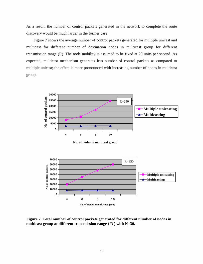
As a result, the number of control packets generated in the network to complete the route

discovery would be much larger in the former case.

Figure 7 shows the average number of control packets generated for multiple unicast and

multicast for different number of destination nodes in multicast group for different

transmission range (R). The node mobility is assumed to be fixed at 20 units per second. As

expected, multicast mechanism generates less number of control packets as compared to

multiple unicast; the effect is more pronounced with increasing number of nodes in multicast

group.

0

5000

10000

15000

20000

25000

30000

4 6 8 10

No. of nodes in multicast group

No.

of c

ontr

ol p

acke

ts

Multiple unicastingMulticasting

R=250

0

10000

20000

30000

40000

50000

60000

70000

4 6 8 10No. of nodes in multicast group

No.

of c

ontr

ol p

acke

ts

Multiple unicastingMulticasting

R=350

Figure 7. Total number of control packets generated for different number of nodes in multicast group at different transmission range ( R ) with N=30.

28

5.5.2 Multicast Efficiency

In ad-hoc network, data from source would reach the destination in multiple hops through

intermediate nodes. In multiple unicast, the same data packets may need to travel through

same set of intermediate nodes in order to reach different destinations. Using multicast, we

intend to avoid this duplication of data traffic which, in turn, reduces the data traffic in the

network. Multicast efficiency, ME, is a measure of reduction in data traffic in the network and

is defined as :

∑for all destinations Number of intermediate nodes in unicast route

ME = −−−−−−−−−−−−−−−−−−−−−−−−−−−−−−−−−−−−−−−−− Number of intermediate nodes in Multicast Route

Going back to the example of figure 1, suppose node A needs to communicate with

{D,G,E}and the three unicast routes to support this communication process are {A, C, D},

{A, C, D, G} and {A, C, D, E}. The same data packets will travel through node C (route 1),

node C and D (route 2) and node C and D (route 3) in order to reach destinations D, G and E.

Thus, if the number of data packets are NUM, the total number of data traffic in the network

would be 5*NUM packets before they reach their destinations. A multicast tree that can

support this communication in one shot is {A, C, D, (G, E)}. Hence the only intermediate

node through which all the data packets would travel is C. Hence, the total data traffic in the

network will be NUM packets before they reach their destinations. So, the multicast

efficiency would be (1+2+2)/1 = 5. This is the best case efficiency; we have not considered

retransmission due to route failure. ME = 1 indicates that there is no difference between

multicast and multiple unicast. This would happen when all the unicast routes are disjoint i.e.

there is no common node among the unicast routes.

Table 5 shows the average Multicast Efficiency for different number of nodes in

multicast group (source + destinations). The node mobility is assumed to be uniform at 20

units per second. In all cases, multicast efficiency is more than one. The improvement is more

significant at low transmission range. The reason is, at higher transmission range (350, for

example), some source-destination pairs are directly connected (single-hop connectivity).

However, at higher transmission range, since the network is more strongly connected (i.e.

each node has more number of neighbors), the control traffic increases the congestion due to

unrestricted propagation of control packets over the network. Subsequently, the delay in

29

delivering the data packets to destinations increases. Hence, low transmission range is a

preferred configuration, where the proposed multicast mechanism shows significant

improvement.

Transmission range

No. of nodes in multicast group

Total no. of intermediate nodes in multiple unicast

Total no. of intermediate nodes in multicast

Multicast Efficiency

4 5 2 2.5 6 9 4 2.25 8 11 4 2.75

250

10 15 6 2.5 4 2 1 2 6 4 2 2 8 6 4 1.5

350 10 7 4 1.75

Table 5. Multicast Efficiency for different number of nodes in multicast group at two transmission ranges

6. Conclusion In this paper, a stability-based distributed routing scheme has been proposed which supports

both unicast and multicast routing in ad hoc wireless networks. The proposed multicast

routing mechanism is a generalized form of a stability-based unicast routing scheme that

relies on determining link stability and path stability in order to find out a stable route from a

source to a destination or to a set of destinations.

From the above discussions, the following points have been observed:

• When the average mobility of all the nodes in the system is low and/or volume of data to

be communicated between source and destination is low, the chance of route error during

data communication with shortest-path algorithm would be low. Conventional shortest

path routing algorithm would work well in this situation.

• When the average mobility of all the nodes in the system is high and/or volume of data to

be communicated between source and destination is high, the chance of route error during

data communication with shortest path algorithm would be high. In this situation, we need

to find out a stable path rather than shortest path for routing. The results show that the

stable-path algorithm reduces route error drastically in all scenarios.

30

• Thus, in order to prevent/reduce route errors, each node should know its affinity with its

neighbors and should be able to evaluate a path for stability. However, there are certain

limitations in the assumptions on calculating affinity in a simulated environment. Since

we have not experimented with physical transceivers, the correctness in predicting

affinity is not beyond doubt. The fluctuation in signal strength of transmitter as perceived

by the receiver in real life scenario may not be due to distance alone. There could be

noise, obstacles, variation in battery power, etc. which would contribute to this

fluctuation. So, predicting the distance between transmitter or receiver or predicting

affinity based on variation in signal strength may not be accurate. However, our prediction

is periodic, so inaccuracy due to random fluctuations can be taken care of. Moreover, it is

a worst-case prediction, so stability cannot be less, in general, than predicted. However,

this worst-case prediction will prevent / reduce route errors, but this will also reduce the

number of communication initiated in stable path algorithm (Table 3). This implies that

even if a path is physically stable to carry a given volume of data, the source will

disregard the path based on calculated stability. A better method for deriving the distance

between a node and its neighbors would be to use GPS system [23]. The use of GPS in the

context of ad hoc network has been proposed earlier[24]. The periodic exchange of

position and velocity information with neighboring nodes only will help a node to

calculate its affinity with its neighbors more accurately. The demonstrated advantages of

stable-path algorithm also justifies the use of GPS in this context, if required.

• Whatever may be the routing scheme, the success of route discovery is critically

dependent on the set of input parameters. Moreover, for a given node density, selecting a

proper transmission range is extremely crucial for the successful operation of an ad hoc

network. A low transmission range will not guarantee proper connectivity among mobile

hosts to ensure effective communication. On the other hand, if the transmission range is

high, it will ensure connectivity but will increase collision and congestion of control

packets, which will increase the end-to-end delay significantly. Hence, the impact of input

parameters for effective operation of an ad hoc network needs to be explored.

31

References 1. Z. J. Haas, Milcom’97 Panel on Ad-hoc Networks,

http://www.ee.cornell.edu/~haas/milcom_panel.html

2. D. B. Johnson and D. Maltz, Dynamic source routing in ad hoc wireless networks, T. Imielinski

and H. Korth, eds., Mobile computing, Kluwer Academic Publ. 1996.

3. Krishna Paul, S. Bandyopadhyay, D. Saha and A. Mukherjee. “A simulation technique for

evaluating a distributed routing scheme among mobile hosts in ad-hoc wireless networks”, Proc of

the 1999 Advanced Simulation Technologies Conference (ASTC'99), April 1999, San Diego,

California, USA.

4. V. D. Park and M. S. Corson, A highly adaptive distributed routing algorithm for mobile wireless

networks, Proc. IEEE INFOCOM ’97, Kobe, Japan, April 1997.

5. C-K Toh, A novel distributed routing protocol to support ad-hoc mobile computing, IEEE

International Phoenix Conference on Computer & Communications (IPCCC’96).

6. R. Dube, C.D. Rais, K. Wang and S.K. Tripathi, Signal stability based adaptive routing for ad hoc

mobile networks, Technical Report CS-TR-3646, UMIACS-TR-96-34, Institute for Advanced

Computer Studies, Department of Computer Science, University of Maryland, College Park, MD

20742, USA, August, 1996.

7. Z.J.Haas, A new routing protocol for the reconfigurable wireless networks, ICUPC’97, San Diego,

CA, Oct. 1997.

8. C. Perkins and P. Bhagwat, Highly dynamic destination-sequenced distance-vector routing for

mobile computers, Proc. of the ACM SIGCOMM, October 1994.

9. S. Murthy and J.J. Garcia-Luna-Aceves, An efficient routing protocol for wireless networks. ACM

Mobile Networks and Application Journal, Special issue on Routing in Mobile Communication

Networks, 1996.

10. S. Corson, J. Macker and S. Batsell, Architectural considerations for mobile mesh networking,

Internet Draft RFC Version 2, May 1996.

11. S.-J. Lee, M. Gerla, and C.-K. Toh, ``A Simulation Study of Table-Driven and On-Demand

Routing Protocols for Mobile Ad-Hoc Networks,'' IEEE Network, vol.13, no.4, July’99, pp.48-54.

12. E. M. Royer and C-K Toh, “A Review of Current Routing Protocols for Ad hoc Wireless

Networks”, IEEE Personal Communication, April 1999, pp. 46-55.

32

13. J. Broch, D. A. Maltz, D. B. Johnson, Y. C. Hu, and J. Jetcheva, "A Performance Comparison of

Multi-Hop Wireless Ad Hoc Network Routing Protocols,' Proc. ACM/IEEE Mobile Comput. and

Network., Dallas, TX, Oct. 1998.

14. S.R. Das, R. Castaneda, J. Yan, and R. Sengupta, ``Comparative Performance Evaluation of

Routing Protocols for Mobile, Ad hoc Networks,'' In Proceedings of IEEE IC3N'98, Lafayette,

LA, Oct. 1998, pp. 153-161

15. K. Obraczka and G. Tsudik, Multicast Routing Issues in Ad Hoc Networks, Proc. of the IEEE

ICUPC ‘98, October 1998.

16. Sung-Ju Lee, William Su, Julian Hsu, Mario Gerla and Rajive Bagrodia, “A Performance

Comparison Study of Ad Hoc Wireless Multicast Protocols”, Proc. Of the IEEE INFOCOM 2000,

Tel-Aviv, 26-30 March, 2000.

17. Ching-Chuan Chiang, Mario Gerla, and Lixia Zhang, Forwarding Group Multicast

Protocol(FGMP) for Multihop, Mobile Wireless Networks, ACM-Baltzer Journal of Cluster

Computing: Special Issue on Mobile Computing, Vol. 1, No. 2, 1998

18. M.Liu, R.R.Talpade, A.McAuley and E.Bommaiah, AMRoute: Adhoc Multicast Routing

Protocol, CSHCN TR 99-1, University of Maryland, USA.

19. J.J.Garcia-Luna-Aceves and E.Lmadruga, A Multicast Routing Protocol for Ad hoc Networks,

Proc. of the IEEE INFOCOM’99,New York, March 1999.

20. C.W.Wu, Y.C.Tay and C-K.Toh, Adhoc Multicast Routing Protocol utilizing Increasing id-

numberS, Internet-draft, draft-ietf-manet-amris-spec-00.txt, November,1998.

21. Sung-Ju Lee, W.Su and M.Gerla, On-Demand Multicast Routing Protocol (ODMRP ) for Adhoc

Networks, Internet-draft, draft-ietf-manet-odmrp-01.txt, June 1999.

22. S. Bandyopadhyay. An Architecture for Distributed Knowledge Processing”, Journal of New

Generation Computing Systems, Vol 4, no.1, 1991.

23. T. Imielinski and J. C. Navas, ``GPS-based Addressing and Routing,'' Tech. Rep. LCSR-TR-262,

CS Dept., Rutgers University, March (updated August) 1996

24. Y-B.Ko and N.H.Vaidya, “Location-aided Routing in Mobile Ad hoc Networks”, Proc. of the

ACM/IEEE MOBICOM 98, Oct. 1998.

33