TSDLMRA: an efficient multicast routing algorithm based on Tabu search
Upload
independentCategory
view
1download
0

For further volumes:http://www.springer.com/series/10028
SpringerBriefs in Computer Science
Series EditorsStan ZdonikPeng NingShashi ShekharJonathan KatzXindong WuLakhmi C. JainDavid PaduaXuemin ShenBorko FurhtVS Subrahmanian


Eric Rosenberg
A Primer ofMulticast Routing

The Author 2012
All rights reserved. This work may not be translated or copied in whole or in part without the written permission of the publisher (Springer Science+Business Media, LLC, 233 Spring Street, New York, NY 10013, USA), except for brief excerpts in connection with reviews or scholarly analysis. Use in connection with any form of information storage and retrieval, electronic adaptation, computer software, or by similar or dissimilar methodology now known or hereafter developed is forbidden. The use in this publication of trade names, trademarks, service marks, and similar terms, even if they are not identified as such, is not to be taken as an expression of opinion as to whether or not they are subject to proprietary rights. Printed on acid-free paper Springer is part of Springer Science+Business Media (www.springer.com)
ISSN 2191-5768 e-ISSN 2191-5776 ISBN 978-1-4614-1872-6 e-ISBN 978-1-4614-1873-3 DOI 10.1007/978-1-4614-1873-3 Springer New York Dordrecht Heidelberg London Library of Congress Control Number: 2011946218
Eric Rosenberg AT&T LabsMiddletown, NJ, USA [email protected]

Preface
This is an introduction to multicast routing, which is the study of meth-ods for routing from one source to many destinations, or from many sourcesto many destinations. Multicast is increasingly important in telecommunica-tions, for such applications as software distribution, video on demand, andfile transfers.
The intended audience of this primer includes
• telecommunication network designers and architects,• researchers in telecommunications and optimization,• upper class undergraduate students, and graduate students, studying com-
puter science, electrical engineering, or operations research.
We assume the reader is familiar with computing a shortest path in a net-work, e.g, by Dijkstra’s method. No prior knowledge of telecommunicationsor routing protocols is assumed, although it will undoubtedly make the read-ing easier. Although a few of the mathematical results are quite deep, theyare presented without proof (but with references to the literature), and canbe skipped with no loss of understanding of subsequent sections.
Both obsolete and currently used methods are examined, in order to pre-vent researchers from reinventing previously proposed methods, and to pro-vide insight into why some methods did become obsolete. The reference listhas over 100 entries. It would not be difficult to find another 100 papersworthy of review or mention. In particular, several areas of multicast arequite active, including wireless multicast, label switched multicast, and ag-gregated multicast. The selection of papers for this primer naturally reflectsboth space considerations and the author’s own interests. In addition to theusual journals and conference proceedings, the IETF web site is a rich sourceof multicast protocol standards and drafts. The web sites of major routervendors are also valuable sources for both protocol descriptions as well asimplementation guidelines and configuration details.
The challenges faced by a small company wishing to implement multicastare typically quite different from the challenges faced by a global serviceprovider. One size does not necessarily fit all when it comes to multicast. Itis hoped that this primer will guide both academic researchers and engineersresponsible for designing and implementing multicast networks.
My sincere thanks to Lee Breslau, Josh Fleishman, Apoorva Karan,Thomas Kernen, Ron Levine, Bob Murray, Han Nguyen, Marco Rodrigues,Samir Saad, Steve Simlo, and especially to Yiqun Cai, Ken Dubose, DonHeidrich, Maria Napierala, Eric Rosen, and Mudassir Tufail, for stimulatingdiscussions and comments on drafts of this primer. Their suggestions havebeen enormously helpful.
Middletown, NJ Eric RosenbergSeptember, 2011
v

vi Preface
About the Author
Eric Rosenberg received a B.A. in Mathematics from Oberlin College anda Ph.D. in Operations Research from Stanford University. He works at AT&TLabs in Middletown, New Jersey (email: [email protected]). Dr. Rosenberg hastaught undergraduate and graduate courses in optimization at Princeton Uni-versity and New Jersey Institute of Technology. He holds seven patents andhas published in the areas of convex analysis and nonlinearly constrainedoptimization, computer aided design of integrated circuits and printed wireboards, and telecommunications network design and routing.

Contents
1 What is Multicast Routing? . . . . . . . . . . . . . . . . . . . . . . . . . . . . . . 11.1 Groups, Sources, and Receivers . . . . . . . . . . . . . . . . . . . . . . . . . . . 21.2 Addressing . . . . . . . . . . . . . . . . . . . . . . . . . . . . . . . . . . . . . . . . . . . . 31.3 The Efficiency of Multicast . . . . . . . . . . . . . . . . . . . . . . . . . . . . . . 51.4 Mathematical Formulation . . . . . . . . . . . . . . . . . . . . . . . . . . . . . . . 61.5 Broadcasting by Flooding . . . . . . . . . . . . . . . . . . . . . . . . . . . . . . . 10
1.5.1 Reverse Path Forwarding . . . . . . . . . . . . . . . . . . . . . . . . . . 111.5.2 RPF with Asymmetric Arc Costs . . . . . . . . . . . . . . . . . . . 13
1.6 The History of Multicast . . . . . . . . . . . . . . . . . . . . . . . . . . . . . . . . 14
2 Basic Concepts in Tree Based Methods . . . . . . . . . . . . . . . . . . . 152.1 Steiner Tree Heuristics . . . . . . . . . . . . . . . . . . . . . . . . . . . . . . . . . . 162.2 Source Trees . . . . . . . . . . . . . . . . . . . . . . . . . . . . . . . . . . . . . . . . . . . 192.3 Shared Trees . . . . . . . . . . . . . . . . . . . . . . . . . . . . . . . . . . . . . . . . . . . 202.4 Redundant Trees for Survivability . . . . . . . . . . . . . . . . . . . . . . . . 222.5 Network Coding . . . . . . . . . . . . . . . . . . . . . . . . . . . . . . . . . . . . . . . . 24
2.5.1 Examples of Network Coding . . . . . . . . . . . . . . . . . . . . . . 252.5.2 Theory of Linear Network Codes . . . . . . . . . . . . . . . . . . . 27
2.6 Encodings of Multicast Trees . . . . . . . . . . . . . . . . . . . . . . . . . . . . 292.7 The Shape of Multicast Trees . . . . . . . . . . . . . . . . . . . . . . . . . . . . 31
3 Dynamic Routing Methods . . . . . . . . . . . . . . . . . . . . . . . . . . . . . . . 353.1 Internet Group Management Protocol . . . . . . . . . . . . . . . . . . . . . 363.2 IGMP Snooping . . . . . . . . . . . . . . . . . . . . . . . . . . . . . . . . . . . . . . . . 373.3 Waxman’s Method . . . . . . . . . . . . . . . . . . . . . . . . . . . . . . . . . . . . . 383.4 DVMRP . . . . . . . . . . . . . . . . . . . . . . . . . . . . . . . . . . . . . . . . . . . . . . 383.5 Multicast OSPF . . . . . . . . . . . . . . . . . . . . . . . . . . . . . . . . . . . . . . . . 403.6 Core Based Trees . . . . . . . . . . . . . . . . . . . . . . . . . . . . . . . . . . . . . . . 423.7 Protocol Independent Multicast . . . . . . . . . . . . . . . . . . . . . . . . . . 44
3.7.1 PIM Dense Mode . . . . . . . . . . . . . . . . . . . . . . . . . . . . . . . . . 453.7.2 PIM Sparse Mode . . . . . . . . . . . . . . . . . . . . . . . . . . . . . . . . 46
vii

viii Contents
3.7.3 BiDirectional PIM . . . . . . . . . . . . . . . . . . . . . . . . . . . . . . . . 523.7.4 Source Specific Multicast . . . . . . . . . . . . . . . . . . . . . . . . . . 55
3.8 Rendezvous Point Advertisement and Selection . . . . . . . . . . . . . 563.8.1 Static RP . . . . . . . . . . . . . . . . . . . . . . . . . . . . . . . . . . . . . . . 563.8.2 Auto RP . . . . . . . . . . . . . . . . . . . . . . . . . . . . . . . . . . . . . . . . 563.8.3 Bootstrap Router . . . . . . . . . . . . . . . . . . . . . . . . . . . . . . . . 573.8.4 Anycast RP . . . . . . . . . . . . . . . . . . . . . . . . . . . . . . . . . . . . . 58
3.9 Comparison of PIM Methods . . . . . . . . . . . . . . . . . . . . . . . . . . . . 593.10 Multipoint Trees using Label Switched Paths . . . . . . . . . . . . . . 59
4 Other Multicast Routing Methods . . . . . . . . . . . . . . . . . . . . . . . . 634.1 Application and Overlay Multicast . . . . . . . . . . . . . . . . . . . . . . . . 634.2 A Gossip Based Method . . . . . . . . . . . . . . . . . . . . . . . . . . . . . . . . . 654.3 Multicasting using Content Addressable Networks . . . . . . . . . . 654.4 Automatic IP Multicast without Explicit Tunnels . . . . . . . . . . . 694.5 Distributed Delay Constrained Multicast Routing . . . . . . . . . . 714.6 Ant-Based Method for Wireless MANETs . . . . . . . . . . . . . . . . . 75
5 Inter-domain and Two-level Multicast . . . . . . . . . . . . . . . . . . . . 775.1 Multiprotocol BGP . . . . . . . . . . . . . . . . . . . . . . . . . . . . . . . . . . . . . 775.2 Multicast Source Distribution Protocol . . . . . . . . . . . . . . . . . . . . 795.3 Two-level Routing using the Yao Graph . . . . . . . . . . . . . . . . . . . 825.4 Two-level Routing using DVMRP . . . . . . . . . . . . . . . . . . . . . . . . 83
6 Aggregate Multicast Trees . . . . . . . . . . . . . . . . . . . . . . . . . . . . . . . . 876.1 Leaky Aggregate Trees . . . . . . . . . . . . . . . . . . . . . . . . . . . . . . . . . . 896.2 Hierarchical Aggregation . . . . . . . . . . . . . . . . . . . . . . . . . . . . . . . . 906.3 Aggregation of Forwarding State . . . . . . . . . . . . . . . . . . . . . . . . . 916.4 Subtree Aggregation . . . . . . . . . . . . . . . . . . . . . . . . . . . . . . . . . . . . 94
7 Multicast Virtual Private Networks . . . . . . . . . . . . . . . . . . . . . . . 977.1 Unicast VPNs . . . . . . . . . . . . . . . . . . . . . . . . . . . . . . . . . . . . . . . . . . 977.2 Draft-Rosen . . . . . . . . . . . . . . . . . . . . . . . . . . . . . . . . . . . . . . . . . . . 100
7.2.1 Default MDT . . . . . . . . . . . . . . . . . . . . . . . . . . . . . . . . . . . . 1017.2.2 Data MDTs . . . . . . . . . . . . . . . . . . . . . . . . . . . . . . . . . . . . . 104
7.3 A General Approach to Multicast VPNs . . . . . . . . . . . . . . . . . . . 1057.4 BGP mVPNs . . . . . . . . . . . . . . . . . . . . . . . . . . . . . . . . . . . . . . . . . . 1067.5 Monitoring Multicast VPN Performance . . . . . . . . . . . . . . . . . . . 1097.6 Empirical Study of Enterprise Multicast Traffic. . . . . . . . . . . . . 110
References . . . . . . . . . . . . . . . . . . . . . . . . . . . . . . . . . . . . . . . . . . . . . . . . . . . . 113

Acronyms
Following the definition is the chapter/section the term is first introduced.
AD auto-discovery 7.3AMT automatic IP multicast without explicit tunnels 4.4AS autonomous system 1.1ASM any source multicast 1.1BGP border gateway protocol 1CAN content addressable network 4.3CBT core based tree 3.6CE customer edge router 7.1DF designated forwarder 3.7.3DVMRP distance vector multicast routing protocol 3.4FIB forwarding information base 3.10GRE generic routing encapsulation 1.4IETF Internet engineering task force 1.1IGMP Internet group management protocol 3.1IGP interior gateway protocol 3.8.4IP Internet Protocol 1.2I-PMSI inclusive provider multicast service instance 7.4ISP Internet service provider 1.1LAN local area network 1.1LFIB label forwarding information base 3.10LSA link state advertisement 3.5LSP label switched path 3.10LSR label switched router 3.10MDT multicast distribution tree 7.2MFIB multicast forwarding information base 6.4MLD multicast listener discovery 3.7.4MOSPF multicast open shortest path first 3.5MP2MP multipoint-to-multipoint 3.10MP-BGP multiprotocol border gateway protocol 5.1MPLS multiprotocol label switching 3.10MSDP multicast source distribution protocol 3.8.4MST minimal spanning tree 1.4MTI multicast tunnel interface 7.2.1MVPN multicast virtual private network 7OIL outgoing interface list 2.2OSPF open shortest path first 1P2MP point-to-multipoint 3.10
ix

x Acronyms
PE provider edge router 7.1PIM protocol independent multicast 2.3PIM-SM PIM-Sparse Mode 3.7.2PMSI provider multicast service instance 7.3RD route distinguisher 7.1RP rendezvous point 2.3RPF reverse path forwarding 1.5.1RT route target 7.1SA source active 5.2SP service provider 7S-PMSI selective provider multicast service instance 7.4SPT shortest path tree 3.7.2SSM source specific multicast 1.1TTL time to live 3.1VPN virtual private network 7VRF virtual routing and forwarding table 7.1
Chapter 1
What is Multicast Routing?
Consider a telecommunications network consisting of a set of nodes con-nected by arcs. The network might be, e.g., the Internet, or the private net-work offered by a service provider such as AT&T. A node represents a phys-ical device, such as a switch or router, connected to other devices. The termswitch is typically used to refer to a device performing layer 2 data link func-tionality (e.g., Asynchronous Transfer Mode (ATM) or Frame Relay) in theOSI model [102], while a router performs layer 3 network functionality in theOSI model. For brevity, by node we mean either a switch or a router. An arcrepresents a communications pathway, such as a fiber optic cable or a radio(wireless) link. Suppose a given source node in the network wishes to sendthe same data stream, composed of packets, to one or more destination nodesin the network. The data stream might be, e.g., an all-employee broadcast,software distribution, a file transfer, financial information, video on demand,or emergency management communications.
We want to determine the path that should be used to send the stream toeach destination node. When there is a single destination node, this problemis known as unicast routing , and is typically solved by computing a shortestpath between the source and the destination. The path might be computedby a link state method such as ISIS [52], Open Shortest Path First (OSPF)[77], or Private Network-Network Interface (PNNI) [8], or by a distance vectormethod such as RIP [68]. (In link state methods, each node has its own viewof the network topology, and computes routes to all destinations; the classiclink-state method is Dijkstra’s method [5]. In distance vector methods, nodesexchange and update routing tables; the classic distance vector method is theBellman-Ford method [5].) The source node forwards each packet to the nextnode on the shortest path, this second node forwards the packet to the thirdnode, and this hop-by-hop forwarding terminates when the packet is receivedby the destination node (a hop is a synonym for an arc). Unicast routing is“easy,” since the complexity of computing a shortest path in a network withN nodes and A arcs is, e.g., O(N2) for Dijkstra’s method for dense networks,and O(A+NlogN) for a Fibonacci heap implementation [5] (a function f(x)is said to be O(g(x)) if there is a positive constant c such that |f(x)| ≤ c |g(x)|for all x ≥ 0).
When the stream is required to be transmitted to every other node in thenetwork, the problem is known as broadcast routing or simply broadcasting.Broadcasting is used, e.g., in ad-hoc mobile networks, where node mobilitycauses frequent link failures [56]. When the stream is required to be transmit-ted to only a specified subset of nodes in the network, the problem is called
E. Rosenberg, A Primer of Multicast Routing, SpringerBriefs in Computer Science, 1 DOI 10.1007/978-1-4614-1873-3_1, © The Author 2012

2 1 What is Multicast Routing?
multicast routing or simply multicasting. Thus unicast is the special cast ofmulticast where there is one destination, and broadcast is the special casewhere all nodes are destinations.
1.1 Groups, Sources, and Receivers
In multicast routing, the basic constructs are sources, receivers, andgroups. A source is an end user that originates a data stream. A receiver is anend user wishing to receive a data stream. Each source is locally connectedto (i.e., subtends) a nearby node, typically either by a direct connection or byan Ethernet Local Area Network (LAN). A source might also be connectedto a second nearby node, in case the connection to the first node, or the firstnode itself, fails. Similarly, each receiver subtends a nearby node, typicallyby a direct connection or Ethernet LAN, and might also be connected to asecond nearby node. We refer generically to an end user source or receiver asa host . There may be no hosts subtending some nodes; such nodes are calledvia nodes.
A multicast group is a set of receivers with a common interest. Note thatthis definition makes no mention of a source. For example, if the group isthe set of students registered for an online course offered by a university,the receivers are the computers of the online students, and the source mightbe the router connected to the video camera in the classroom where theinstructor is teaching, A second example is a financial institution such asa brokerage house, where the group is the set of stock traders, distributedaround the globe, who communicate with each other about stock offerings.The set of receivers is the entire set of computers used by the traders; sinceeach trader typically needs to send financial data to other traders, the set ofsources is also the entire set of computers used by the traders.
In the first example, there is a single source, and the set of receivers isrelatively static for the duration of the online lecture, since students mustpre-register for the online course (although some students might sign-in lateor sign-off early). In the second example, both the set of sources and theset of receivers are dynamic, depending on which traders are working thatday, or are interested in some stock offer. The financial institution mighthave multiple multicast groups, e.g., one for bond traders and one for stocktraders.
In the any source multicast (ASM) model [31], there is no limit on thenumber of multicast groups, or on the number of sources and receivers fora group. (While the ASM model assumes no limits, in practice equipmentvendors may impose limits due to, e.g., processing or memory limitations.)Group membership is dynamic; receivers can join or leave a multicast groupat any time. Similarly, the set of sources for a group can vary over time.
1.2 Addressing 3
Sources and receivers can be physically located anywhere in the network. Anyhost can be a source or receiver for a multicast group. A given receiver cansimultaneously join multiple groups, and a given source can simultaneouslysend to multiple groups. A source is not required to know the location oridentities of receivers, and a source for a group need not join the group.
A refinement of the ASM model, called source specific multicast (SSM) andstudied in Section 3.7.4, allows, for a given group g, a receiver to select thespecific sources for this g from which it will receive a stream. SSM prevents areceiver from being deluged with streams from all sources for a given group,and the paths generated with SSM have delay no larger, and may be smaller,than the paths generated with ASM. We assume the ASM model throughoutthis primer, except where SSM is specifically discussed.
Typically, in a small geographic area like a university campus, the hostsare interconnected by a multi access subnet (e.g., a LAN), and the subnetalso connects one or more routers. One of the routers on the subnet will bethe primary router, and connections from the subnet to the outside world arevia the primary router. Usually a secondary router is configured to take overif the primary router fails. We say that the active router is the local routerfor any source or receiver host on the subnet.
The Internet contains a very large number of Autonomous Systems (ASs),where an AS is a set of one or more networks administered by the sameorganization, e.g., a government, corporation, or university. A given AS isadministered by only one organization. However, a given organization, e.g.,an Internet Service Provider (ISP), might administer multiple ASs. We alsouse the term domain to refer to an AS. The Internet Engineering Task Force(IETF) is the organization that issues standards documents that specify thealgorithms and procedures used for routing in the Internet and in VirtualPrivate Networks (Chapter 7).
1.2 Addressing
Although Layer 2 protocols such as Frame Relay and ATM can supportmulticast, currently the vast majority of multicast is over Layer 3 networksrunning the Internet Protocol (IP). For IP Version 4 (IPv4) networks, a mul-ticast group is identified by a 32 bit IP address confined to a specific range.The 32 bits in each IPv4 address are divided into 4 octets of 8 bits each, soeach octet can express a (decimal) number from 0 to 255. Address assignmentis controlled by the Internet Assigned Numbers Authority (IANA) [50].
An address prefix A/N consists of an IP address A and an integer mask N ,and represents the set of IP addresses whose leftmost (i.e., most significant) Nbits match the first N bits in the binary expansion of A. For example, considerthe address prefix 209.12.0.0/15. Since the address has the binary expansion

4 1 What is Multicast Routing?
11010001.00001100.00000000.00000000, the address prefix represents any IPaddress of the form 11010001.0000110x.xxxxxxxx.xxxxxxxx, where “x” is thewild card (either 0 or 1). Thus this IP prefix represents IP addresses in therange 209.12.0.0 to 209.13.255.255. This is illustrated in Table 1.1, where byte1 is the leftmost byte.
byte 1 byte 2 byte 3 byte 4Address 11010001 00001100 00000000 00000000Mask 11111111 11111110 00000000 00000000Prefix 11010001 0000110x xxxxxxxx xxxxxxxx
Table 1.1 Address prefix
For IPv4, the first (i.e., leftmost) 4 bits of the first octet of a multicastgroup address must be 1110, so the multicast address range is 224.0.0.0 to239.255.255.255. An address in this range is known as a class D address [77].Some class D addresses are reserved for special purposes [23]. For example,the group address 224.0.0.5 sends to all routers in an OSPF domain. Ad-dresses in the range 224.0.1.0 to 238.255.255.255 are called globally scopedaddresses, and are used when the multicast groups span various organiza-tions and the Internet. Addresses in the range 232.0.0.0/8 are reserved forSource Specific Multicast. Thus the first 8 bits of any address in this rangemust be (decimal) 232, and the remaining 24 bits can be anything. Addressesin the range 239.0.0.0/8 are called limited scope or administratively scopedaddresses, and are used when the multicast group has a limited span, such asa single university or company [24]. An organization using administrativelyscoped addresses typically configures its routers to prevent traffic (i.e., a datastream) with this group address from being sent outside the organization. Ingeneral, a group address does not convey any geographic information, sincethe group sources and receivers may be scattered around the globe.
A host wishing to send to multicast group g uses the IP address of g asthe destination address. When a source sends a stream to a multicast group,the source address of each packet in the stream is the unicast address of thesource. For IPv4 networks, the source address is also a 32 bit address, whichmust lie outside of the range reserved for multicast addresses. Since the poolof available IPv4 addresses is rapidly dwindling, 128 bit IP Version 6 (IPv6)addresses have been introduced. For IPv6 multicast addresses, the first octetmust be 0xFF (i.e., binary 11111111). Any other value for this octet identifiesthe address as a unicast address. IPv6 multicast addresses are defined in [47],and the rules for assigning new IPv6 multicast addresses are defined in [44].
GLOP [70] is a multicast addressing method for IPv4 networks. Curiously,GLOP is not an acronym; it does not stand for anything. The term was simplycreated to refer to this addressing method. For a four octet IPv4 address,GLOP sets the first octet to 233, sets the second and third octets to the 16bit Autonomous System number [102], and the last octet is locally assigned.

1.3 The Efficiency of Multicast 5
1.3 The Efficiency of Multicast
Suppose a given source node s wishes to send a stream of bandwidth b toa set of k other nodes in a network. One way to accomplish this is to have screate k copies of the stream, and send each of the copies to its destinationusing unicast. This approach, known as unicast replication, is particularlyefficient when b and k are small; in this case the extra node overhead andbandwidth required for replication may more than compensate for not havingto implement a multicast routing protocol. Similarly, if the streams are verybursty (frequent periods of inactivity between packets), then the overhead ofrepeatedly building and tearing down trees argues for replication.
Alternatively, we can create a tree, rooted at s, connected to each of the kdestinations. Replication of the data stream occurs only at branching pointsof the tree. For example, consider Figure 1.1, which shows a network of 10nodes interconnected by 9 arcs. Suppose the source node s is node 1, which
Fig. 1.1 Multicast vs. unicast
must send a data stream of bandwidth b to nodes 4, 5, 6, 8, 9, 10. Withunicast routing, node 1 would need to send 6 copies of the data stream, sothe total bandwidth on arc (1, 2) would be 6b; the total bandwidth on arcs(2, 3) and (2, 7) would be 3b, and the total bandwidth on each of the otherarcs would be b. With multicast, node 1 sends a single copy of the streamto node 2, which creates 2 copies of the stream. One copy goes to node 3,which creates 3 copies (for nodes 4, 5, 6), and one copy goes to node 7, whichcreates 3 copies (for nodes 8, 9, 10). This illustrates the bandwidth savingsin the network with multicast. An additional advantage of a tree over unicastreplication is that, with unicast replication, node 1 must manage 6 outgoingstreams, rather than 1 outgoing stream with a tree. Similarly, node 2 mustmanage 6 outgoing streams with the unicast approach; with a tree, node 2manages only 2 outgoing streams. Since incremental memory and processing

6 1 What is Multicast Routing?
is required for each stream managed by a node, a tree may lessen the burdenon nodes relative to unicast replication.
1.4 Mathematical Formulation
Consider a directed network (N ,A), where N is the set of nodes andA is the set of arcs. We associate with arc a ∈ A a non-negative cost ca.We also denote by (i, j) the directed arc from node i to node j; the cost ofthis arc is cij . A directed network formulation allows for the general caseof asymmetric arc costs (i.e., cij �= cji); if all costs are symmetric, then anundirected network formulation is appropriate. We use the terms networkand graph interchangeably. Two nodes are adjacent or neighbors if they areconnected by a single arc. A node n ∈ N is a leaf node if exactly one arc isincident to (i.e., touches) n.
A path between two nodes s and t is an ordered sequence of p arcs(s, n1), (n1, n2), · · · , (np−2, np−1), (np−1, np) such that np = t. If s = t andp ≥ 2 then the path is a cycle; i.e., a cycle is a path of two or more arcs form-ing a loop. The graph (N ,A) is connected if there is a path between eachpair of nodes; it is complete if there is an arc between each pair of nodes. Thecost of a path is the sum of the arc costs, taken over all arcs in the path. Apath between nodes s and t is a shortest path if its cost is less than or equalto the cost of any other path between s and t. The diameter of (N ,A) ismax{c�(i, j) | i ∈ N , j ∈ N}, where c�(i, j) is the length of the shortest pathbetween nodes i and j.
A subgraph (N , A) of (N ,A) is a graph such that N ⊆ N , A ⊆ A, andeach endpoint of an arc in A belongs to N . A tree in (N ,A) is a connectedsubgraph with no cycles. The cost of a tree is the sum of the arc costs overall arcs in the tree. A spanning tree of a connected graph (N ,A) is a tree(N , A) where A ⊆ A; i.e., the tree uses a subset of the arcs in A and spansthe nodes in N . A minimal spanning tree (MST) of a connected graph (N ,A)is a spanning tree whose cost is less than or equal to the cost of any otherspanning tree of (N ,A).
Let Z ⊂ N . A Steiner tree over (N ,A,Z) is a tree that uses nodes in N ,arcs in A, and spans the nodes in Z. Define N − Z to be those nodes in Nbut not in Z. Nodes in N − Z used in the Steiner tree are called Steinerpoints. Figure 1.2 illustrates a spanning tree of an undirected graph, andalso a Steiner tree with Z = {A, B, C, D, E}. In the Steiner tree picture, thenodes U , V , and W are Steiner points.
In telecommunications, the concept of an interface is important. An inter-face is the endpoint of a logical or physical communications channel betweentwo nodes. For example, a 1 Gbps (gigabits per second) Ethernet port (phys-ical point of connection on a router) might be divided into 5 interfaces, each

1.4 Mathematical Formulation 7
Fig. 1.2 Spanning and Steiner trees
of bandwidth 200 Mbps (megabits per second), and these 5 interfaces mightconnect to different devices (e.g., interfaces 1-3 might connect to neighboringrouters, while interfaces 4 and 5 might connect to subtending hosts). Thesedifferent interfaces could be assigned different costs. A given arc a connectingnodes n1 and n2 will have an interface (say i1) on n1 and an interface (sayi2) on n2. Thus each interface on a node is an endpoint of a distinct arcoriginating or terminating at the node. The interface identifier is local to anode, so that two different nodes might both have an interface labelled i1.
A tunnel in a network is a logical path between two nodes. Suppose u ∈ N ,v ∈ N , but (u, v) �∈ A. Suppose we want specially marked packets (e.g.,all packets with a specific source host address) that arrive at u to take aspecified tunnel to v. The path taken by this tunnel might be the shortestpath between u and v, or it might not be, e.g., if the tunnel is designed toutilize only special high bandwidth arcs. Each node on this tunnel, exceptfor v, stores the knowledge of the next node on the tunnel. Multiple tunnelscan be configured between the same pair of nodes, e.g., to provide enhancedsecurity by sending traffic for different customers over different tunnels.
With a Generic Routing Encapsulation (GRE) tunnel [39], an inner packetis encapsulated in an outer packet at one end of the tunnel, and the outerpacket is sent to the remote end. At the remote end, the encapsulation isremoved and the inner packet is then processed or forwarded as required.With GRE tunnels, the inner packet is not processed by via routers (routersbetween the tunnel endpoints), and the tunnel is treated as any other arc bythe IP routing protocol.
Another type of tunnel, called a label switched path, is illustrated in Fig-ure 1.3. Suppose we want to tunnel between u and v using the bold arcs illus-trated on the left. The tunnel can be created by encapsulating each packetthat arrives at u by placing it in another packet with an outer label. For ex-ample, in Figure 1.3, suppose that each packet arriving at u with source hostaddress s is encapsulated and given the outer label L1. Node u consults its

8 1 What is Multicast Routing?
Fig. 1.3 A label switched path tunnel
label forwarding table to learn that any packet with outer label L1 should besent to w. Upon arriving at w, the label forwarding table at w specifies that,if a packet arrives at w with outer label L1, then L1 should be swapped with(i.e., replaced by) L2 and then the encapsulated packet should be sent to x.Similarly, at x, label L2 is swapped for L3, and the packet is sent to y. At y,label L3 is swapped for L4, and the packet is sent to v. The forwarding tableat v instructs it to now decapsulate any encapsulated packet with outer labelL4, at which point the decapsulated packet is available for further processing,e.g., to be forwarded to a directly attached receiver host.
We are now ready to define the multicast routing problem. We assumethat each source host s subtends the single node n(s) ∈ N , and that eachreceiver host r subtends the single node n(r) ∈ N . We say that s subtends oris behind node n(s), and similarly for n(r). Under this assumption, to routeto a receiver host r, it suffices to route to n(r). Similarly, to route from asource host s, it suffices to route from n(s). We say that node n ∈ N is usedby multicast group g if there is a receiver host behind n that has joined g,in which case we say that n is a receiver node for g. Similarly, we say that anode n ∈ N is used by g if there is a source host behind n for g, in whichcase we say that n is a source node for g. Each node will in general be usedby multiple groups, and a given node can be both a source and receiver nodefor a group.
For group g, let R(g) be the set of receiver nodes for g, and let S(g) bethe set of source nodes for g. For example, if g is a broadcast group, thenR(g) = N . Note that the definition of R(g) is independent of the identity ofthe source host sending to g; we will later consider SSM, for which the setof receiver nodes depends on (s, g), that is, on both g and the source hosts of packets for g. Let G be a set of multicast groups. The multicast routingproblem is to determine, for each g ∈ G and each s ∈ S(g), a path from s toall the nodes in R(g).
An alternative definition of this static problem was given by Waxman [110],who refers to a set of nodes to be interconnected in a multipoint connection,rather than to a source sending to a set of receivers. For a given group g andsource node s used by g, define Z = {s} ∪ R(g). Then the static problem ofconnecting the nodes in Z with minimal cost is the problem of computinga minimal cost Steiner tree over (N ,A,Z). Note that our definition of the

1.4 Mathematical Formulation 9
multicast routing problem assumes the set of arcs in the network is specified;we are not computing a network design/topology for a given set of nodes,e.g., as in [96]. Also, even though some applications require more bandwidththan others (e.g., video streaming compared with stock price information),we will not, in this primer, be concerned with the bandwidth of the arcs inthe network and the bandwidth required by the multicast application.
Waxman [110] also states a dynamic version of this problem. The probleminput data is a network, and a sequence of requests, where each request is toeither add or delete a node from a multipoint connection. The objective is todetermine a corresponding sequence of minimum cost trees, such that tree kinterconnects all the nodes in the multipoint connection following request k.If we allow the routing to be re-optimized after each request, this dynamicversion is equivalent to a sequence of independent static problems.
The unicast routing table for node n ∈ N specifies, for each destination (anode or subnet or address prefix) known to n, the outgoing arc or interface onthe shortest path from n to that destination. Given two nodes x and y on atree rooted at s, we say that y is downstream of x if x is on the shortest pathin the tree from s to y. The multicast routing table specifies, for each groupg known to n, the set of outgoing arcs over which a replica of an incomingpacket should be sent in order to reach the downstream receivers for g. Forexample, in Figure 1.1, suppose nodes {3, 4, 5, 8, 9, 10} are receiver nodes forsome g, and node 1 is the source node for g. Then the multicast routing tableat node 2 for g specifies the outgoing arcs {(2, 3), (2, 7)} for packets arrivingfrom node 1, the multicast routing table at node 3 for g specifies the outgoingarcs {(3, 4), (3, 5} for packets arriving from node 2, and the table at node 7 forg specifies the outgoing arcs {(7, 8), (7, 9), (7, 10)} for packets arriving fromnode 2.
Although this primer is mostly concerned with networks with fixed po-sition nodes and arcs, there is a large literature on mobile ad-hoc networks(MANETs). A MANET is set of mobile nodes which communicate over sharedwireless channels, without any fixed network infrastructure or central networkmanagement. Such networks are used in, e.g., emergency search and rescue,and in military battlefields. Each mobile node participates in an ad hoc rout-ing protocol by which it discovers nearby nodes and creates multihop pathsthrough the network. Since the transmission range of each node is limited,multiple hops might be necessary to send a stream; each mobile node actsas both a host and a router that forwards packets. Since battery life is amajor concern, multicast routing protocols for MANETs are often concernedwith minimizing power consumption. A large number of methods have beenproposed for multicast routing in a MANET; see Chen and Wu [21] and Jun-hai, Danxia, Liu, and Mingyu [56], which surveys 32 schemes and providesa taxonomy for grouping these methods. We review one MANET scheme inSection 4.6.

10 1 What is Multicast Routing?
1.5 Broadcasting by Flooding
An easy but inefficient method for broadcasting is flooding . A simple flood-ing method starts with the source node sending a packet to each of its neigh-bors. Each node receiving the packet in turn forwards the stream to each ofits neighbors, except that the packet is not forwarded to the neighbor fromwhom the packet was received. With such a scheme, it is necessary to preventpackets from cycling around the network, being continuously retransmitted.One way to accomplish this is to include a hop count in each packet. Thesource initializes this value to a large value, e.g., the network diameter asmeasured in hop count, with each arc cost set to 1. Each node processing thepacket decrements the value by 1; when the value reaches 0, the packet isdiscarded. Since the diameter may not be known a priori, the upper bound|N | − 1 can be used, where |N | is the number of elements in N .
The above procedure can be improved by preventing a node from redis-tributing the multiple copies it may receive of a packet. For example, con-sidering Figure 1.4, suppose the source a must send a stream to nodes b, c,d, and e. Node a will send a copy of each packet to b and c, which in turn
Fig. 1.4 Improved flooding
send it to d, so d receives two copies of each packet. However, d needs to sendonly one copy of each packet to e. To accomplish this, the source can markeach copy of a given packet with the same packet identifier; each downstreamnode will then process only the first packet received with a given identifier,and discard the other packets with the same identifier. Having each node re-tain knowledge of the identifier of processed packets simultaneously preventspackets from cycling indefinitely, and prevents multiple copies of the samepacket from being retransmitted by a given node [81]. (This rule is used inContent Addressable Network method described in Section 4.3.) Formally,this method is described as follows. Let N (n) be the set of nodes adjacent ton, i.e., reachable in one hop from n. First, the source node s sends a packetto each of its neighbors. Each node n receiving the packet executes the pro-cedure in Figure 1.5. If there are multiple sources that wish to flood packets,the identifiers imposed by each source node must be globally unique. This can

1.5 Broadcasting by Flooding 11
procedure F lood&Mark()1 if the packet was not previously processed by node n {2 Let n be the node from which the packet was received;3 Send the packet to each n ∈ N (n) except n;4 Mark the packet as processed by n;5 }6 else discard the packet;
Fig. 1.5 Flood&Mark
be achieved, e.g., by having the identifier imposed by s contain the globallyunique address of s.
Flooding explores all possible paths between the source and destinationnodes, so a packet will reach a destination node as long as one path is avail-able. This makes flooding robust and well-suited to networks prone to nodeor arc failures. However, flooding is bandwidth intensive, since each packet isretransmitted to all neighbors except for the neighbor from whom the packetwas received [101].
1.5.1 Reverse Path Forwarding
The next multicast routing improvement we consider is reverse path for-warding (RPF), first proposed in 1977 by Dalal [27]. This technique is appli-cable to general multicast routing, not just broadcasting. Consider a sources for group g that is sending packets to a set of receivers that have joinedg. Suppose some node n receives a packet on arc a and must decide whatto do with the packet. The reverse path forwarding (RPF) check is: if theshortest path from n to s uses arc a, the check passes, and n should forwardthe packet on each of the arcs specified in its multicast forwarding table forgroup g; otherwise, the check fails and n should discard the packet. The uni-cast routing table at n is used to determine if arc a is on the shortest pathfrom n to s. If the unicast routing method has found more than one minimalcost route, a tie-breaking mechanism (e.g., a hash function) will select one ofthem.
What distinguishes RPF from unicast forwarding is that RPF forwardingdepends on the source node, while unicast forwarding depends on the des-tination node. For example, consider Figure 1.6. Suppose the shortest path(using unicast routing) from n to s uses arc a. If n receives a packet on theincoming arc a then the RPF check passes, since a is on the shortest pathfrom n to s; the packet is replicated at n and sent out, say, on arcs c, d, and

12 1 What is Multicast Routing?
Fig. 1.6 Basic RPF check
e, as specified in the multicast routing table at n for g. The packet is not sentback out over a, since a packet is never sent back out on the arc over whichit arrived. If n receives a packet on the incoming arc b then the RPF checkfails, since b is not on the shortest path from n to s; the packet is discarded.
As observed by Perlman [84], the RPF check, though quite simple, greatlyreduces the overhead of flooding. Since a node n accepts a given packet onlyon one incoming arc, then n forwards this packet (on each of the interfacesin its multicast forwarding table) only once, and the packet traverses any arcin the network at most once.
With RPF, the decision whether to drop a packet is made only after thepacket has been replicated and sent to a neighboring node. Consider an arc abetween node i and an adjacent node j. Suppose a is not on the shortest pathfrom j to the source. The RPF check says that j should drop a packet arrivingfrom i on a. Since the packet will be dropped by j, there is no reason for ito send the packet to j. The extended RPF check of Dalal and Metcalfe [28]says that i should send a packet to a neighbor j along arc a only if a is on theshortest path from j to the source. Node i can easily determine if this holds ina link state multicast routing protocol, or even in a distance vector protocol,if each neighbor advertises its upstream next hop [98]. The extended RPFcheck is illustrated in Figure 1.7, where the cost of four undirected arcs isshown. The basic RPF check says that if x receives from w a packet originated
Fig. 1.7 Extended RPF check
by s, the packet should be discarded since (x, w) is not on the shortest pathto s. The extended RPF check says that w should never forward the packet

1.5 Broadcasting by Flooding 13
to node x, since (x, w) is not on the shortest path from x to s. This extendedRPF check, however, has not proved to be popular in practice.
1.5.2 RPF with Asymmetric Arc Costs
If the arc costs are asymmetric, which is often the case in the Internet,the shortest path from a source node s to a receiver node t will in generalnot be the same as the shortest path from t to s. The validity of the RPFmethod for broadcasting does not require the assumption of symmetric arccosts [28]. However, the RPF method can cause multicasting to fail, unlessalgorithmic enhancements are made. This is illustrated in Figure 1.8 for thetrivial case of one source node s and one receiver node t. The arc a1 has cost1 in the direction t → s and cost 3 in the reverse direction, and the arc a2 hascost 2 in both directions. Anticipating the PIM-based protocols discussed in
Fig. 1.8 RPF with asymmetric costs
Section 3.7, suppose node t sends, via shortest path unicast, a join requestto s that any packets sourced by a host subtending s should be sent to t.This request will take arc a1. When s heeds the request and sends to t usingshortest path routing, packets will take arc a2. If t uses the RPF check, itwill discard all packets sent by s. There are at least two solutions to thisdilemma.
One solution is for t to know the incoming interface that will be taken bypackets following the shortest path from s to t. This approach, proposed in2008 by Li, Mirkovic, Ehrenkranz, Wang, Reiher, and Zhang [66], requiresthe join request sent from a receiver node t to a source node s to followthe same path that s would use to send to t using shortest path routing.Implementation of this method requires each node n to store, for each entryin its forwarding table, the forward interface into n that would be used bypackets taking the shortest path from that entry (now treated as a source)to n. The request sent by n to join a tree rooted at some source node s cannow be sent along a sequence of forward interfaces, and this path (the trueshortest path from s to n) is used by s to send packets down to n. (Thismethod can also be used to detect spoofing, where the source of a packet isdeliberately forged, e.g., to create denial of service attacks.)

14 1 What is Multicast Routing?
A second approach takes the opposite tack, and requires that the pathtaken by packets sent from a source node s to a receiver node t take thesame path as the shortest path from t to s. This is the approach adoptedby PIM-based multicast protocols. The drawback of this approach is that,if the arc costs are asymmetric, the path taken by packets sent from s to tmay not be the shortest path from s to t; the path is only guaranteed to bethe shortest path from t to s. This possibility of non-optimal routing has notprevented PIM-based protocols from being widely adopted.
1.6 The History of Multicast
As the reader now has a glimpse into multicast, we provide a very fewwords on its history. The groundwork for Internet multicast was laid by Deer-ing in his 1991 Ph.D. dissertation [32]. The first large scale multicast deploy-ment began in 1992, with the MBone (Multicast Backbone). The MBone usedunicast encapsulated tunnels to connect a set of small multicast networks.These tunnels allowed multicast traffic to traverse Internet routers that werenot multicast enabled. IP Multicast traffic was encapsulated upon entry to atunnel, and sent using unicast to the destination end of the tunnel, where itwas decapsulated. The MBone grew from 40 subnets in 4 countries in 1992 to2800 subnets in 25 countries by 1996 [98]. In 1997, work began on a hierarchi-cal approach to inter-domain multicast. In this approach, different multicastprotocols could be used in each domain, domains exchange information onmulticast sources, and intra-domain trees are connected by an inter-domaintree. By 1999, there were two Internet2 backbone multicast networks, vBNSand Abilene, which began to supplant the MBone.
In the 1990s there was intense focus on multicast routing methods (seethe 1997 review by Diot, Dabbous, and Crowcroft [35], and the 2000 reviewby Almeroth [6]). In a 2006 survey by Oliveira, Pardalos, and Resende [81]of optimization problems related to multicast, 64% of the references were topapers published between 1992 and 1998, and only 18% are 2000 or later.However, multicast has enjoyed a resurgence of interest, due the ability ofservice providers to now offer reliable, scalable multicast in the Internet andin Virtual Private Networks (Chapter 7).

Chapter 2
Basic Concepts in Tree Based Methods
Tree based approaches distribute packets along a tree. The tree is logical,but not necessarily physical; the routing follows a tree but the underlyingphysical network topology (e.g., the fiber optic cables) need not have a treetopology. Each node maintains, for each multicast group g, a multicast rout-ing table for g, which specifies which interfaces are part of the tree for g.For example, consider Figure 2.1, which shows the tree for a particular g.The solid arcs are in the tree, and the dotted arcs are in the physical net-
Fig. 2.1 Multicast tree
work, but not in the tree. Suppose h1, h2, and h3 are both receiver hosts andsource hosts for g. Let An(g) denote the interface list at node n for group g.We have AA(g) = {(A, C), (A, h1)}, AB(g) = ∅, AC(g) = {(C, A), (C, D)},AD(g) = {(D, C), (D, E), (D, F ), (D, h2)}, etc. If A receives a packet fromh1 and the RPF check passes, then A examines AA(g) and sends the packetout (A, C). If A receives a packet from C and the RPF check passes, thenA sends it out on (A, h1). Similarly, if D receives a packet from h2 and theRPF check passes, then D sends it out on (D, C), (D, E), and (D, F ), whileif D receives a packet from E and the RPF check passes, D sends it out on(D, C), (D, F ), and (D, h2). Thus a packet for g arriving at node n whichpasses the RPF check is replicated and sent out on each interface in An(g)except the incoming interface.
Due to practical considerations, use of a tree does not eliminate the needfor an RPF check. Consider Figure 2.2, where S is the source node. Supposeconvergence of the unicast routing tables has not yet occurred, so that Athinks that B is its RPF neighbor (i.e., the next node on the shortest pathfrom A to the source node S), B thinks that C is the RPF neighbor, and C
E. Rosenberg, A Primer of Multicast Routing, SpringerBriefs in Computer Science, DOI 10.1007/978-1-4614-1873-3_2, © The Author 2012
15

16 2 Basic Concepts in Tree Based Methods
Fig. 2.2 RPF check with nonconvergence
thinks that A is the RPF neighbor. Then any packets sourced by A caughtin the A → C → B → A loop will cycle until they time out. However, untilconvergence has occurred, the RPF check at A will prevent any new packetsfrom S from entering the A → C → B → A loop [90].
2.1 Steiner Tree Heuristics
One approach to tree based methods is to construct, for each g, a Steinertree which spans the nodes in S(g) ∪ R(g) (the set of source and receivernodes for g). The problem of computing a minimum cost Steiner tree isNP-complete [42], and there is a large literature on exact and approximatealgorithms for constructing minimal cost Steiner trees (see, e.g., the survey byWinter [113]). The algorithms can be classified as centralized or distributed.Centralized methods incorporate full information about the topology of thenetwork. In decentralized methods each node independently makes routingdecisions based upon a limited or summarized view of the network topology.Centralized methods typically utilize either Prim’s or Kruskal’s MST method.In Prim’s 1957 method, the tree is initialized as any given node. In eachiteration the node closest to the tree, and the arc from the tree to that node,are added to the tree; the method terminates when all nodes have been addedto the tree. In Kruskal’s 1956 method, each node is initially its own subtree,and in each iteration the lowest cost arc connecting two subtrees is added,until all nodes are in a single tree [5].
A popular centralized heuristic for building Steiner trees is the methodof Kou, Markowsky, and Berman (KMB) [64]. Given the undirected graphΨ = (N ,A) and a set Z ⊂ N of nodes to interconnect, Step 1 is to considerthe auxiliary complete undirected graph Δ = (Z, E), where there is one arcin E for each (unordered) pair of nodes in Z. The cost of (i, j) ∈ E is thecost of the shortest path, in the original graph Ψ , between nodes i and j.Corresponding to each arc (i, j) ∈ E is a path in Ψ between nodes i andj. Step 2 is to compute an MST of Δ (if the MST is not unique, pick onearbitrarily). Step 3 is to construct a subgraph of Ψ by replacing each edge inthe MST by its corresponding shortest path in Ψ . Step 4, the final step, is

2.1 Steiner Tree Heuristics 17
to create a Steiner tree T by deleting arcs from the subgraph so that all leafnodes of T belong to Z. It can be shown [64] that the cost of the Steiner treecomputed by this method is no more than twice the cost of the minimal costSteiner tree.
The method is illustrated in Figure 2.3. Step (0) shows the starting graphΨ , and Z = {A, E, F }. Next to each arc is the arc cost. Step (1) showsthe auxiliary graph Δ with the shortest path distance between each pair ofnodes in Z. In Step (2), the MST of Δ is chosen. In Step (3), the arc (A, E)in Δ corresponds to the path A → B → D → E in Ψ (other paths withcost 4 could have been chosen), and arc (A, F ) in Δ corresponds to the pathA → C → D → F in Ψ (other paths could have been chosen). An MST ofthe subgraph is chosen in Step (4), and the final pruning is done in Step (5).For this example, the method yields an optimal (minimal cost) Steiner tree.
Fig. 2.3 KMB Steiner tree
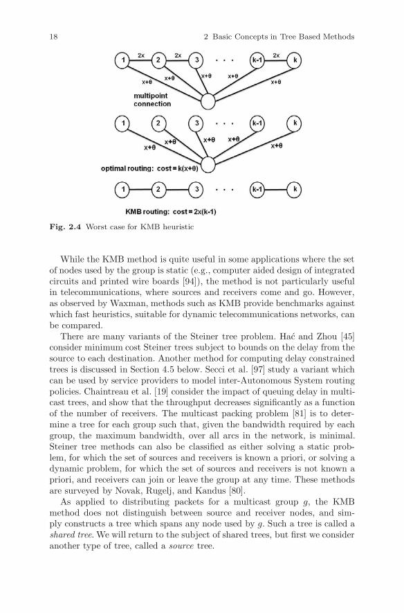
Waxman [110] provides an example where, for this method, the worst casebound of twice the optimal cost is approached. In Figure 2.4, top picture,the nodes 1, 2, · · ·, k are to be interconnected. For 0 < θ << 1, the optimaltree is shown in the middle picture, while the lower picture shows the treegenerated by the KMB method. Since [2x(k − 1)]/[k(x + θ)] → 2 as k → ∞and θ → 0, the worst case ratio of 2 is asymptotically achieved. Waxmanalso compares the KMB method against other Steiner tree heuristics, usinga random graph model in which an arc between two nodes is created withprobability βe−d/(Lα), where d is the distance between the two nodes, L isthe maximum distance between any two nodes, α ∈ (0, 1], and β ∈ (0, 1].Increasing β yields more arcs, while decreasing α increases the frequencyof short arcs relative to longer arcs. (This random model has been utilizedextensively by subsequent researchers.)
18 2 Basic Concepts in Tree Based Methods
Fig. 2.4 Worst case for KMB heuristic
While the KMB method is quite useful in some applications where the setof nodes used by the group is static (e.g., computer aided design of integratedcircuits and printed wire boards [94]), the method is not particularly usefulin telecommunications, where sources and receivers come and go. However,as observed by Waxman, methods such as KMB provide benchmarks againstwhich fast heuristics, suitable for dynamic telecommunications networks, canbe compared.
There are many variants of the Steiner tree problem. Hac and Zhou [45]consider minimum cost Steiner trees subject to bounds on the delay from thesource to each destination. Another method for computing delay constrainedtrees is discussed in Section 4.5 below. Secci et al. [97] study a variant whichcan be used by service providers to model inter-Autonomous System routingpolicies. Chaintreau et al. [19] consider the impact of queuing delay in multi-cast trees, and show that the throughput decreases significantly as a functionof the number of receivers. The multicast packing problem [81] is to deter-mine a tree for each group such that, given the bandwidth required by eachgroup, the maximum bandwidth, over all arcs in the network, is minimal.Steiner tree methods can also be classified as either solving a static prob-lem, for which the set of sources and receivers is known a priori, or solving adynamic problem, for which the set of sources and receivers is not known apriori, and receivers can join or leave the group at any time. These methodsare surveyed by Novak, Rugelj, and Kandus [80].
As applied to distributing packets for a multicast group g, the KMBmethod does not distinguish between source and receiver nodes, and sim-ply constructs a tree which spans any node used by g. Such a tree is called ashared tree. We will return to the subject of shared trees, but first we consideranother type of tree, called a source tree.

2.2 Source Trees 19
2.2 Source Trees
Consider a group g, and a source host s for g, where s subtends the sourcenode n(s). A source tree for (s, g) has n(s) as the root of the tree, and spansthe set of nodes wishing to receive the (s, g) stream, i.e., the stream sent by sto group g. A source tree is in general also a Steiner tree, since it may containnodes not used by g. Packets only flow down the tree (away from the root),from the source to the receivers, and never up a source tree towards the root.The source tree is identified by the pair (s, g).
For a rooted tree, the upstream neighbor, also called the RPF neighbor,of node n is the neighbor of n that is on the shortest path from n to theroot. For a source tree, the root is the source node. Referring to Figure 2.5,suppose for some group g1 there are source hosts s1 and s2 behind node1, and suppose that behind nodes 3, 4, 6, 7, and 9 are hosts wishing toreceive the (s1, g1) stream. The (s1, g1) source tree is rooted at node 1, andis drawn using heavy solid lines. The upstream neighbor of node 7 is node3, the upstream neighbor of node 3 is node 2, and the upstream neighbor ofnode 2 is the source node 1. At node 1 the outgoing interface list (OIL) for
Fig. 2.5 Source tree
(s1, g1) is A1(s1, g1) = {(1, 2), (1, 4)}, so packets sourced by s1 are replicatedat node 1, and send to nodes 2 and 4. At node 2 we have A2(s1, g1) ={(2, 3), (2, 6)}. At node 6 one we have A6(s1, g1) = {(6, 9), (6, r3)}. At node9, we have A9(s1, g1) = {(9, r6), (9, r7)}. At each node on the source tree,the RPF check is used to determine whether an incoming packet should bereplicated and sent over all arcs in the OIL, or the packet should be discarded.
Each node on the (s1, g1) tree is said to maintain state for (s1, g1). InFigure 2.5, nodes 1, 2, 3, 4, 6, 7, and 9 each maintain (s1, g1) state. Note thatnode 2 maintains (s1 , g1) state even though there are no subtending receiver

20 2 Basic Concepts in Tree Based Methods
hosts wanting the (s1, g1) stream. The state information includes the interfaceleading to the RPF neighbor, and the set of downstream arcs, as specified bythe OIL. For example, node 2 stores the upstream arc (2, 1) leading to theRPF neighbor (node 1), and A2(s1, g1).
Now suppose that, for the same group g1, there is another source host s2
behind node 1, and that behind nodes 3, 4, 6, 7, and 9 are hosts wishing toreceive the (s2, g1) stream. We now create another source tree, the (s2, g1)tree. This source tree might use exactly the same set of arcs as the (s1, g1)tree, or it could be designed using different methods, and not use the sameset of arcs (e.g., if the tree construction method is bandwidth aware, and thestreams generated by s1 and s2 have different bandwidths). This new sourcetree is an (s2 , g1) tree, (s2, g1) state is created on each node on this tree, andeach node stores the interface to the RPF neighbor and the (s2 , g1) OIL.
Suppose now that host s3, subtending node 8, is the source for a differentgroup g2, and the receiver nodes for (s3, g2) are 3, 4, 5, 6, and 7. The arcs fora (s3, g2) source tree, rooted at node 8, are shown in heavy dotted lines. Wehave A8(s3, g2) = {(8, 4), (8, 5), (8, 9)}, A9(s3, g2) = {(9, 7), (9, r6), (9, r7)},and similarly for the other nodes on the (s3, g2) tree. The RPF neighbor ofnode 8 is itself (it is the root), the RPF neighbor of node 9 is node 8, etc. Eachnode on the (s3, g2) tree maintains (s3, g2) state, and stores the interface tothe RPF neighbor and the (s3, g2) OIL.
When the number of sources and groups is large, considerable memory canbe required at each node to store, for each (s, g) tree touching the node, the(s, g) pair, the interface to the RPF neighbor, and the outgoing interface list.The memory requirement can be greatly reduced by using shared trees.
2.3 Shared Trees
A shared tree for a group g is a single tree used by all sources for g. Sharedtrees were first proposed by Wall [109] in 1980, and further developed in 1993by Ballardie, Francis, and Crowcroft [10] who called them core based trees(CBTs). The incarnation of shared trees popular today is Prototcol Indepen-dent Multicast - Sparse Mode (PIM-SM), developed by Estrin et al. in 1997([37], [38]). CBTs are studied in Section 3.6 and PIM-SM in Section 3.7.2.Another type of shared tree, BiDirectional PIM, is studied in Section 3.7.3.Shared trees mitigate some of the scaling problems (consumption of memory,bandwidth, or node processing resources) of source trees.
Since there is no source node to serve as the root of a shared tree, oneprivileged node serves at the root. For CBTs, this node is called a core;for PIM-SM it is called a rendezvous point (RP). An RP and a core servethe same function. They are typically chosen in the middle of the geographicregion spanned by the group sources and receivers (e.g., if the multicast group

2.3 Shared Trees 21
spans the U.S., the core or RP might be in Kansas). Figure 2.6 illustrates,using heavy lines, a shared tree, rooted at node 5, for a group g. There are
Fig. 2.6 Shared tree
source hosts for g behind nodes 1, 3, and 9, and receiver hosts behind nodes2, 4, 6, and 7. Since a shared tree for group g is used for any source host forg, the tree is represented by the pair (�, g), where � denotes the “wild card,”meaning it matches any source host for the group. Thus (�, g) state appearson each node spanned by the shared tree, whether or not a source host orreceiver host subtends the node. We have (�, g) state on all nodes except 8and 10. The RPF neighbor of node 7 is node 3, the RPF neighbor of node3 is node 2, and the RPF neighbor of node 2 is node 5. Similarly, the RPFneighbor of node 9 is node 5, etc.
One disadvantage of shared trees, compared to source trees, is the potentialfor non-optimal routing. The example in Figure 2.4 above illustrates this,since for the tree generated by the KMB method (lower figure), the worstcase cost between any two nodes is 2x(k − 1), while for small θ the worstcase cost in the optimal Steiner tree (middle figure) is 2(x + θ). Even witha minimal cost shared tree, non-optimal routing can occur, as the followingsimple example demonstrates. Consider a group g and three nodes a, b, andc, at the vertices of an equilateral triangle, with unit arc costs. Suppose thereis a source host and a receiver host for g behind each node. Suppose the(�, g) shared tree is {(a, b), (b, c)}. Then each node has the single state (�, g).Traffic from a to c will follow the path a → b → c, with cost 2. If instead weuse source trees, we would generate three trees, one rooted at each node, andeach node would have three (s, g) states. Packets from a to c would followthe path a → c on the tree rooted at a, with a path cost of 1.
As a final example, referring to Figure 2.6 above, suppose all arc costs are1. Then the optimal route from s3 to the receiver host behind node 6 is thesingle hop (9, 6). However, the route on the shared tree is the path 9 → 5 toreach the RP/core, and then the path 5 → 2 → 3 → 6 down the shared tree

22 2 Basic Concepts in Tree Based Methods
to reach node 6. This example also illustrates that the location of the coremay greatly impact the path length and latency (i.e., delay) for a multicaststream.
2.4 Redundant Trees for Survivability
In case of a node or arc failure in a tree, it is important to quickly establisha new tree. Various schemes for this are surveyed by Bejerano, Busi, Ciavaglia,Hernandez-Valencia, Koppol, Sestito, and Vigoureux [12]. One method, ap-plicable to source trees, is to specially construct two trees, rooted at the samesource node s and spanning the same set of receiver nodes. The two trees havethe following property: if a node (other than the source) fails, then for anyother node n there is a path, on one of the trees, from s to n. The methoddescribed in [12] has two main steps. First, a subgraph Ψ is created whichcontains two node disjoint paths from the root to every other node. Second,two directed trees, with the desired property, are constructed from arcs in Ψ .
The desired subgraph Ψ can be constructed from the original undirectedgraph (N ,A) as follows. The initial step is to construct an ear, which is acycle of length at least 3 containing the source s. So create any such cycle,and traversing the cycle in an arbitrary direction from s, let S1 be the orderedset of nodes in the cycle. For example, in Figure 2.7, sub-figure (i), wheres = 0, we let S1 = {0, 1, 4, 0}. If S1 = N we are done, since the cycle containstwo disjoint paths from s to each node on the cycle. Otherwise, pick a node
Fig. 2.7 Redundant trees - node ordering

2.4 Redundant Trees for Survivability 23
n ∈ N − S1 and construct two node disjoint paths from s to n, using, e.g.,the classic method of Surballe [103]. Let u be the node in S1 that is on oneof the disjoint paths from s to n, such that u is closest to n. Let v be thenode in S1 that is on the other disjoint path from s to n, such that v isclosest to n. Without loss of generality, assume S1
u ≤ S1v , where S1
u = j ifu is in position j of the ordered set S1. (It might be that S1
u = S1v if, for
example, u = v = s.) Starting from u, we traverse the path from u to n tov, and suppose, excluding u and v, this path encounters the ordered set ofnodes Q2. (Q2 is the ear connecting n to S1.) We insert the ordered set Q2
into S1 just before position v, yielding the new ordered set S2. In Figure 2.7,sub-figure (ii), we select n = 6, yielding u = 1, S1
u = 2 (i.e., “1” is in thesecond position of the array S1), v = 4, S1
v = 3 (i.e., “4” is in the thirdposition of the array S1), and Q2 = {2, 5, 6}; inserting Q2 before v in S1
yields S2 = {0, 1, 2, 5, 6, 4, 0}. If S2 = N we are done, otherwise we select anode n ∈ N − S2, create an ear Q3 connecting n to S2, etc.
Continuing the example, in sub-figure (iii) we select n = 8 yielding u = 5,S2
u = 4, v = 6, S2v = 5, Q3 = {7, 8}; inserting Q2 before v in S2 yields
S3 = {0, 1, 2, 5, 7, 8, 6, 4, 0}. Finally, in sub-figure (iv) we select n = 9 yieldingu = 2, S3
u = 3, v = 8, S3v = 6, Q3 = {3, 9}; inserting Q3 before v yields
S4 = {0, 1, 2, 5, 7, 3, 9, 8, 6, 4, 0}. Let S� be the final ordered set (containingall the nodes) created by this procedure. Then |S�| = N +1, where N = |N |,since the root s appears in the first and last positions, and all other nodesappear exactly once. We now use S� to create the two directed trees.
We create the first directed tree T1 as follows. For n ∈ N , n �= s, pickone node pn such that the undirected arc (pn, n) exists in the original graph(N ,A), and such that pn appears after n in the ordered set S�; add thedirected arc (pn, n) to T1. Continuing our example, Figure 2.8 shows how
Fig. 2.8 Redundant trees - tree creation
the indices pn are selected to create T1. In the center of the figure are theelements of the ordered set S�, and below the node numbers we show, foreach n, n �= s, the selection of pn used to create T1. Starting from the next tolast position of S�, for node 4 we pick p4 = 0, yielding the directed arc (0, 4);

24 2 Basic Concepts in Tree Based Methods
for node 6 we pick p6 = 4, yielding the directed arc (4, 6); for node 8 we pickp8 = 6, yielding the directed arc (6, 8); and we continue this way, generatingthe directed arcs (8, 9), (9, 3), (8, 7), (7, 5), (5, 2), and (2, 1). Note that therule for creating this tree may allow multiple choices for pn for some n, so T1
is not uniquely determined. Figure 2.9, sub-figure (i) shows T1.
Fig. 2.9 Redundant trees - final step
We create the second directed tree T2 as follows. For each node n ∈ N ,n �= s, pick one node pn such that the undirected arc (pn, n) exists in theoriginal graph (N ,A), and such that pn appears before n in the ordered setS�; add the directed arc (pn, n) to T2. In Figure 2.8, above the node numberswe show, for each n, n �= s, the selection of pn used to create T2. Starting fromthe second position of S�, for node 1 we pick p1 = 0, yielding the directedarc (0, 1); for node 2 we pick p2 = 1, yielding the directed arc (1, 2); andwe continue this way, generating the directed arcs (2, 5), (5, 7), (2, 3), (3, 9),(7, 8), (5, 6), and (5, 4). The tree T2 also is in general not uniquely determined.Figure 2.9, sub-figure (ii) shows T2.
Consider any node n. Tree T1 contains a path from s to n that uses onlyarcs touching nodes which appear in S� after n. Tree T2 contains a path froms to n that uses only arcs touching nodes which appear in S� before n. Hence,if some node fails, there will either be a path in T1 from s to n, or a path inT2 from s to n.
2.5 Network Coding
In multicast routing, a node receives a packet on an incoming interface,and replicates the packet, sending it on a set of outgoing interfaces. In uni-cast routing, there is a single outgoing interface, so no replication is needed.With both approaches, the payload in each packet is unchanged, and only therouting information (e.g., the outgoing interface list) changes as the packetis forwarded. With network coding, introduced in a seminal 2000 paper by

2.5 Network Coding 25
Ahlswede, Cai, Li, and Yeung [4], a node receiving packets over several in-coming interfaces generates new packets by operating on the bits receivedover these incoming interfaces. Network coding can provide improved band-width utilization, lower delay, and, for wireless networks, reduced number oftransmissions.
2.5.1 Examples of Network Coding
The following three examples from Sprintson [100] illustrate these benefits.In all these examples, we assume that all packets have the same fixed length,that all arcs have unit capacity (each arc can send one packet per unit time),that there is no delay for bits to traverse a node, and that nodes have infinitecapacity.
Considering first Figure 2.10, sub-figure (i), suppose that source s1 wants
Fig. 2.10 Network coding - first example
to send packet x to t1 and t2, and source s2 wants to send packet y to t1and t2. The only directed tree available to s1 is illustrated in solid linesin sub-figure (ii), and the only directed tree available to s2 is illustratedin solid lines in sub-figure (iii). However, s1 and s2 cannot both use thesetrees simultaneously, since arc (u, v) has capacity 1. Using network coding, asshown in sub-figure (iv), node u computes x⊕ y, which is defined as follows.Assume the packet is k bits long. Then x⊕ y is the packet of length k whosei− th bit is xi ⊕ yi, where xi ⊕ yi = 1 if xi + yi = 1 and 0 otherwise. Node usends x⊕ y to v, who sends it to t1 and t2. Destination t1 can recover y fromx and x ⊕ y since, e.g., if xi = 1 and xi ⊕ yi = 0, then yi = 1. Similarly, t2can recover x from y and x⊕ y. So, with network coding, s1 can send x overthe tree rooted at s1 at the same time s2 sends y over the tree rooted at s2,even though the trees share a common arc.

26 2 Basic Concepts in Tree Based Methods
The second example, shown in Figure 2.11, illustrates delay reduction usingnetwork coding. We define the depth of a tree to be the number of arcs inthe longest path from the root to a leaf. Considering sub-figure (i), suppose
Fig. 2.11 Network coding - second example
source s must send packets x and y to destinations t1, t2, and t3. Suppose suses the tree in sub-figure (ii) to send x and the tree in sub-figure (iii) tosend y. Since the depth of the first tree is 2 and the depth of the second treeis 3, it takes three time units for the three destinations to receive both x andy (this holds for any choice of arc disjoint trees). With network coding as insub-figure (iv), only two time units are required for the three destinations toreceive either x and y, or x and x ⊕ y, or y and x ⊕ y.
The last example shows how network coding can reduce the number ofwireless transmissions. Considering Figure 2.12, sub-figure (i), suppose umust send packet x to v, and v must send packet y to u. Without network
Fig. 2.12 Network coding - third example
coding, four transmissions are required. With network coding, as shown in

2.5 Network Coding 27
sub-figure (ii), only three transmissions are required. Note that, since this iswireless transmission, it counts as one transmission when n sends x ⊕ y toboth u and v in sub-figure (ii).
2.5.2 Theory of Linear Network Codes
The following discussion is based upon Sprintson [100]. The theory utilizesthe rules of arithmetic over a finite field GF (q). For our purposes, it sufficesto let GF (q) be the set of nonnegative integers less than q, for some primenumber q, so if for some integers α and β we have 0 ≤ α < q and 0 ≤ β < q,then α + β is defined to be their sum (mod q).
Consider a directed tree rooted at s, and suppose s needs to send k packets(p1, · · · , pk) to D destination leaf nodes. Without loss of generality, we canassume that each of the D destination nodes has k incoming arcs (if thisdoes not hold for some destination d, we can create a new destination d andk directed arcs from d to d).
For a given node n, let I(n) be the set of incoming arcs at n and let J (n)be the set of outgoing arcs at n. We reserve the first k arc indices for the arcsincoming to s, so I(s) = {1, 2, · · ·, k}. If for n ∈ N we have |I(n)| > 1 (i.e.,more than one incoming interface), then we select |I(n)| · |J (n)| coefficientsfij such that i ∈ I(n), j ∈ J (n), and fij ∈ GF (q). For example, if q = 2 thefield is GF (2), and if n has 3 incoming interfaces and 2 outgoing interfaces,then we generate 6 binary coefficients for this n. If n has exactly one incomingarc i, each arriving packet is duplicated and sent out over each outgoing arc;in this case we set fij = 1 for j ∈ J (n). This coefficient generation is donefor each node n. We denote by {fij} the set of all the coefficients for all thenodes.
Suppose node n receives packet pi on incoming arc i ∈ I(n), and let pj
be the packet sent on outgoing arc j ∈ J (n). Then, for j ∈ J (n), the linearnetwork code generated by the coefficients {fij} is defined as
pj =∑
i∈I(n)
fijpi ,
where the arithmetic operations are performed componentwise on each packet,and arithmetic is modulo q. Thus, for example, referring to Figure 2.13, whereeach arc is numbered, the packet p3 sent out from s on arc 3 is f13p1 +f23p2,the packet p4 sent out from s on arc 4 is f14p1 +f24p2, and the packet p9 sentout from c on arc 9 is f69p6 +f79p7 = f69p3 +f79p4. Since the packet sent oneach outgoing arc from n is a linear combination, using the {fij} coefficients,of the packets on the incoming arcs to n, it follows that the packet sent oneach arc leaving a node is a linear combination of the k packets received by

28 2 Basic Concepts in Tree Based Methods
the source node s. In our example, we have, for the arcs 5 and 10 into t1,
Fig. 2.13 Network coding - coefficients
p5 = p3 = f13p1 + f23p2 (2.1)
p10 = p9 = f69p6 + f79p7 = f69(f13p1 + f23p2) + f79(f14p1 + f24p2). (2.2)
Define
P =
(p1
p2
)
and
M1 =
(f13 f23
f13f69 + f14f79 f23f69 + f24f79
).
Then ( 2.1) and ( 2.2) can be written as
(p5
p10
)= M1 P.
Similarly, for the arcs 8 and 11 into t2 we have, for some 2 by 2 matrix M2,
(p8
p11
)= M2 P.
Destination t1 can determine P from (p5, p10) if and only if M1 is non-singular, or equivalently, if the determinant det(M1) is nonzero. Similarly, t2can determine P from (p8, p11) if and only if M2 is non-singular, or equiv-alently, if det(M2) is nonzero. Each of these determinants is a multivariatepolynomial in the variables fij. The problem is thus to determine values forthe fij variables that make det(M1) and det(M2) nonzero. It can be shownthat, if det(M1) det(M2) is not identically zero, then it is possible to find

2.6 Encodings of Multicast Trees 29
values of fij such that det(M1) det(M2) �= 0 whenever the size q of the finitefield GF (q) exceeds the maximum degree of det(M1) det(M2) with respectto any variable fij. Although the example of Figure 2.13 is for k = 2 (twoincoming arcs at s), the results hold for any k and for any number D ofdestinations, so for d = 1, 2, · · · , D we generate a k by k matrix Md which isrequired to be non-singular.
One method, called random network coding, generates {fij} by choosingeach fij from a uniform distribution over GF (q) for a sufficiently large q. Itcan be shown that, with this method, the probability of obtaining a set {fij}that makes each Md non-singular is (1 − D
q)β , where β is the total number
of fij variables. We refer the reader to the books and articles surveyed in[100] for more details on how to determine the required q and deterministicmethods (including a polynomial time algorithm) for computing the {fij}.Also, bounds can be derived on the improvement of the information trans-mission rate using network coding, compared to not using it. The Avalanchefile distribution protocol [71] has been implemented using random networkcoding.
2.6 Encodings of Multicast Trees
Consider a multicast group g with only a few receivers. If the receivers aregeographically dispersed over the network, (�, g) or (s, g) state will be createdon many nodes as flows travel to the receiver nodes. To avoid this, Arya,Turletti, and Kalyanaraman [7] in 2005 proposed encoding the multicast treewithin every packet in a flow for g, thus completely eliminating creating (�, g)or (s, g) state in the network for this flow. With this approach, multicastforwarding is accomplished by reading and processing packet headers. It alsocan reduce control overhead, while allowing real-time updating of the tree incase of a node or arc failure.
The multicast tree encoding must be of near minimal length, since it isincluded in each packet, and the processing of the encoding must be compu-tationally simple. The representation can either specify (i) only the receivernodes (behind which are receiver hosts for g), or (ii) the entire sequence ofnodes in the tree; (ii) can be useful for traffic engineering, to take a specifiedpath.
For the Link � encoding described in [7], each arc has a unique index. Theencoding has two components, (i) a balanced parentheses representation ofthe tree, and (ii) a preorder (depth first) list of the arc indices. The encodingis constructed by a preorder tree traversal: when an arc is visited for the firsttime, its arc index and a “(” are written, and when the arc is revisited aftervisiting all arcs in its subtree, a “)” is written. For a tree with L arcs, thisrepresentation requires 2L parentheses and L arc indices. Figure 2.15 shows

30 2 Basic Concepts in Tree Based Methods
the encoding for the full tree of Figure 2.14, and for the subtrees rooted at Q,D, and F ; for clarity, the arcs represented by each encoding are also listed.In the forwarding of a packet, each node receives only the encoding of itssubtree. A forwarding node reads the balanced parentheses once to identifyits outgoing arcs and the encoding of subtrees to be forwarded to its children.
Fig. 2.14 Tree encoding example
Fig. 2.15 Multicast tree encoding

2.7 The Shape of Multicast Trees 31
2.7 The Shape of Multicast Trees
In this section we present both empirical and theoretical results describingthe shape of multicast trees. Several metrics can be used to describe a setof trees, including (i) depth, (ii) degree frequency (the percentage of nodeswith degree j, for j = 1, 2, · · ·), and (iii) average degree (the expected valueof the degree frequency distribution). One motivation for such studies is therecognition that, relative to unicast routing, there is increased complexity indesigning and maintaining multicast networks, and that this complexity istypically justified by the savings in bandwidth, which is a function of theshape of the multicast tree. Another motivation is that, when designing arouting protocol, it is sometimes necessary to make assumptions about thetopology of the networks over which the protocol will run.
We can study the topology of multicast trees in the Internet from twoperspectives: (i) each node in the tree represents a router, and an arc in thetree represents a physical connection between two routers, or (ii) we mapthe actual multicast tree into an AS-tree, where each node in the AS-treerepresents an AS containing one or more routers in the actual tree, and an arc(i, j) exists in the AS-tree if there is at least one physical connection betweena router in AS i and a router in AS j in the actual tree. Since multicasttrees are dynamic, as receiver and source hosts appear and disappear, anyempirical study is necessarily a snapshot in time.
In the early 2000s, there was considerable effort to characterize multicasttrees observed in actual networks. This work is reviewed by Chalmers andAlmeroth [20]. Many results showed the following power law relationship.Consider a tree with R receiver hosts and N nodes. Let Lm be the totalnumber of arcs in the tree. Suppose we find a unicast path between each pairof nodes in the tree; let Lu be the total number of arcs in all these unicastpaths. Let Lu = Lu/[(N)(N−1)/2], so Lu is the average path length, in hops,between any two nodes in the tree, Chuang and Sirbu [22] showed empiricallythat Lm/Lu = Rα for some constant α, where 0 < α < 1 (typically, α ≈0.8). This and other early studies ([85], [108]) used simulated networks, andassumed receivers were uniformly distributed in space, rather than usingactual Internet data.
Define the efficiency δ of the multicast tree as δ = 1 − Lm/Lu. As δapproaches 0, the cost of unicast and multicast are nearly equal, so there islittle bandwidth savings from multicast. (A trivial example with δ = 0 is atree with a single arc.) As δ approaches 1, multicast becomes more efficient.A highly efficient multicast network is given in Figure 2.16, which shows 2clusters connected by a single arc. Since Lu is O(K2) and the multicast treehas Lm = 2K + 1 arcs, we have 1 − (Lm/Lu) → 1 as K → ∞.
Following [20], using Lm/Lu = Rα we write Lm/Lu = sεRα−1, where
Lu = sεLu/R, and where sε is a scaling factor (sε ≈ 1) introduced since therelationship between Lu and Lu is not exact. This yields δ = 1−sεR
ε, where

32 2 Basic Concepts in Tree Based Methods
Fig. 2.16 Multicast efficiency
ε = α − 1, which provides a measure of multicast efficiency as a function ofthe number of receiver hosts. For α = 0.8 we have ε = −0.2; the typical rangefor ε is -0.38 to -0.27. Empirical results in [20] show that this relation holdsunder a wide range of behavior of receiver hosts. The formula implies that forgroups with as few as 20 to 40 receiver hosts, multicast uses 55%-70% fewerarcs than unicast. A difference between [22] and [20] is that, if J receiver hostsare connected to a leaf node, in [22] this counts as 1 receiver host, while in[20] this counts as J receiver hosts. Another power law relationship given in[20] relates the number of N of nodes in the tree to the number R of receiverhosts: N = sτRτ , where typically τ ∈ (0.66, 0.72).
Phillips, Sheker, and Tangmunarunkit [85], seeking to explain the powerlaw Lm/Lu = Rα observed by Chuang and Sirbu, assume the network isa V -ary tree (each node except the leaf nodes has V descendants), of depthD = logV N . They showed that Lu ≈ R(D+1/ln V −ln R/ln V ), which is nota power law. The question was then taken up by Adjih, Georgiadis, Jacquet,and Szpankowski ([1], [2]). Define a = R/N . They observed that the resultsin [22] show a phase transition at a = 1: for a � 1 we have Lm/Lu = αRβ
for some α > 0 and some β ≈ 0.8, and as R → ∞ with N fixed, the plot ofLm/Lu flattens out. The first model studied in [2] is the same V -ary modelused in [85]. For 1 ≤ k ≤ D, there are a total of V k arcs connecting nodes atlevel k − 1 to nodes at level k, and the probability that such an arc is in thetree after R receiver hosts have been selected is 1−(1−V −k)R. The expectednumber of arcs in the tree is thus
Lm(R) =
D∑k=1
V k(1 − (1 − V −k)R
).
For a << 1, they show that
Lm(R)
Lu≈ R
(1 +
1 − γ
lnN+
lnV
2 lnN− lnR
lnN− lnV
lnNψ(V, ln a)
),
where ln denotes natural logarithm, γ is the Euler constant 0.571 . . ., and|ψ(V, x)| < 0.153 for all x and V < 1000. For a → ∞, they show that

2.7 The Shape of Multicast Trees 33
Lm(R)
Lu=
N
D
(V
V − 1− e−a
)− V
V − 1− 1
2
(ae−a + aV e−aV
)+ O
(1
lnR
).
The second model studied in [2] also assumes a V -ary tree of depth D,where all receivers are connected to leaf nodes. However in this model, thesingle arc between a node at level k and the adjacent node at level k − 1 isreplaced by a concatenation of a random number of arcs, with no branchingat intermediate nodes. Let nk be the average number of arcs inserted betweenlevels k and k − 1, and assume that nk = φnk−1, where 0 ≤ φ ≤ 1. Define θby φ = V −θ. This is illustrated in Figure 2.17, for θ = 1 and D = 3, wheretwo nodes (smaller, not shaded) are inserted into each arc between levels 0and 1, and one node is inserted into each arc between levels 1 and 2. With
Fig. 2.17 Self similar tree
this refinement, the average path length for a unicast connection is now
Lθu =
D∑k=1
V (D−k)θ =Nθ−1
V θ − 1,
and the expected number of arcs in the multicast tree is
Lθm(R) =
D∑k=1
V (D−k)θV k(1 − (1 − V −k)R
).
For a ≈ 0, we obtain the power law
Lθm(R)/Lθ
u ≈ c1R1−θ − c2
for some constants c1 and c2, where c1 and c2 are independent of R and N .As a → ∞ with N fixed, all leaf nodes belong to the multicast tree, so Lθ
m ap-proaches (NV 1−θ−NθV 1−θ)/(V 1−θ−1), which is the total number of links inthe full multicast tree. Moreover, Lθ
m(R)/Lθu shows a phase transition around

34 2 Basic Concepts in Tree Based Methods
a = 1, in agreement with the empirical results of [22]. Although these resultsassumed receivers are attached only to leaf nodes, similar results hold whenthe model is extended to allow receivers to connect to non-leaf nodes that arebranching nodes. Random trees are also studied in [16], which derives func-tional equations that can be used to estimate the advantage of multicast overunicast, based upon the tree branching distribution, the fraction of networknodes that are multicast enabled, and the number and location of receiverhosts.
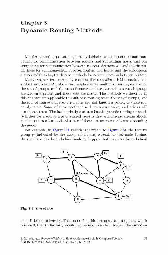
Chapter 3
Dynamic Routing Methods
Multicast routing protocols generally include two components, one com-ponent for communication between routers and subtending hosts, and onecomponent for communication between routers. Sections 3.1 and 3.2 discussmethods for communication between routers and hosts, and the subsequentsections of this chapter discuss methods for communication between routers.
Many Steiner tree methods, such as the centralized KMB method de-scribed in Section 2.1 above, are applicable to multicast routing only whenthe set of groups, and the sets of source and receiver nodes for each group,are known a priori, and these sets are static. The methods we describe inthis chapter are applicable to multicast routing when the set of groups, andthe sets of source and receiver nodes, are not known a priori, or these setsare dynamic. Some of these methods will use source trees, and others willuse shared trees. The basic principle of tree-based dynamic routing methods(whether for a source tree or shared tree) is that a multicast stream shouldnot be sent to a leaf node of a tree if there are no receiver hosts subtendingthe node.
For example, in Figure 3.1 (which is identical to Figure 2.6), the tree forgroup g (indicated by the heavy solid lines) extends to leaf node 7, sincethere are receiver hosts behind node 7. Suppose both receiver hosts behind
Fig. 3.1 Shared tree
node 7 decide to leave g. Then node 7 notifies its upstream neighbor, whichis node 3, that traffic for g should not be sent to node 7. Node 3 then removes
E. Rosenberg, A Primer of Multicast Routing, SpringerBriefs in Computer Science, DOI 10.1007/978-1-4614-1873-3_3, © The Author 2012
35

36 3 Dynamic Routing Methods
arc (3, 7) from its outgoing interface list (OIL) for group g. This is known aspruning node 7 from the tree. Suppose the receiver host behind node 6 alsodecides to leave g. Then node 6 informs node 3 that traffic for g should notbe sent to node 6, so arc (3, 6) is deleted from the (�, g) OIL at node 3. Nownode 3 is a leaf node of the tree. Since there are no receiver hosts behindnode 3 itself, then 3 informs its upstream neighbor, node 2, that traffic for gshould not be sent to node 3, so node 2 deletes arc (2, 3) from the (�, g) OILat node 2. This process continues until no further pruning can be done.
Suppose now nodes 6, and 7, and 3 have been pruned from the tree forgroup g, and a host behind node 6 decides to rejoin g. First, the host informsnode 6 that it is rejoining g. Then node 6 must rejoin the tree, so node 6 tellsnode 3 to send traffic for g down to node 6, so node 3 adds arc (3, 6) to its(�, g) OIL. Finally, node 3 tells node 2 to send traffic for g down to node 3,so node 2 adds (2, 3) to its (�, g) OIL.
3.1 Internet Group Management Protocol
Once a host learns about the existence of a multicast group (e.g., throughan email or web site) it uses the Internet Group Management Protocol(IGMP) to announce its desire to join the group. A host wishing to join groupg sends an IGMP membership report to its local router. In turn, routers lis-ten to the IGMP messages sent by hosts on a directly attached subnet, andperiodically determine which multicast groups have at least one interestedreceiver host on the subnet. If there are multiple routers on a subnet, oneof them, called the designated router, is elected to perform these functions.To query the hosts on a subnet, IGMP uses the all-hosts broadcast address224.0.0.1 and a Time to Live (TTL) value of 1, which means that queries arenot forwarded beyond the attached subnet. Upon receiving a query, a hostsends a report listing each multicast group to which it belongs. When a hostfirst joins a group, it immediately informs its local router. This ensures that,if the host is the first group member on the subnet, it immediately receivesgroup traffic, without waiting for a router query.
When a router on a subnet determines that there have been no locallyattached hosts interested in some group g for a specified time period, therouter will stop forwarding packets for g to that subnet. The drawback ofthis approach is that, even if none of the hosts on a subnet want traffic for g,traffic will be forwarded until a specified period has elapsed, which is a wasteof bandwidth and router resources. IGMP Version 2 provides a faster methodto let a router know that it should stop forwarding traffic for g to a subnet:a host may inform its local router, using an IGMP leave group message, thatit does not want traffic for g. Upon hearing such a message, the router willinitiate a query to determine if any host on the subnet wants traffic for g;

3.2 IGMP Snooping 37
if no host does, then the router stops forwarding that traffic. Version 2 alsoallows a router to query for membership in a specific multicast group, ratherthan having attached hosts report on membership for all the groups to whichthey belong. Finally, IGMP Version 3 allows a host to inform its local routerthat it is interested in traffic for group g, but only for a specific set of sourcesfor this group. If the host indicates interest in a group g but does not specifya set of sources for g, traffic from any source for g will be forwarded to thehost. Similarly, IGMP Version 3 can allow a host to specify, for g, a set ofsources from which it does not want to receive traffic. IGMP Version 3 isused with Source Specific Multicast (Section 3.7.4).
IGMP is only for IPv4; the IPv6 equivalent of IGMP is Multicast ListenerDiscovery (MLD) Version 2 (IETF RFC 3810).
3.2 IGMP Snooping
Suppose that, instead of a set of hosts being directly connected to a router,they instead connect to a Layer 2 switch (e.g., an Ethernet switch), and theEthernet switch connects to the router. A Layer 2 switch receiving a multicastpacket for group g will, by default, send it to all attached hosts, even if thesehosts have not signalled, using IGMP, their desire to receive packets for g.IGMP snooping at the switch can be used to stop the forwarding of packetsto hosts uninterested in g.
With IGMP snooping, the switch examines the Layer 3 information in theIGMP packets exchanged between the hosts and the router. When the switchhears the IGMP membership report for g from some host, the switch addsthe host’s port (i.e., interface) number to the switch’s multicast table entryfor g. Similarly, when the switch hears the IGMP leave group report for gfrom some host, the switch deletes the host’s port number from the switch’smulticast table entry for g.
With IGMP Version 2, because IGMP membership report and leave groupmessages are transmitted as multicast packets, these messages cannot be dis-tinguished from multicast data. Therefore the switch must examine everymulticast data packet to see if it contains an IGMP membership report orleave group message. This may severely degrade the performance of the switchprocessor, especially for high bandwidth multicast data streams. To mitigatethis, the IGMP checks can be performed using specially designed hardware,rather than using software or firmware. This issue disappears with IGMP Ver-sion 3, which sends IGMP reports to the fixed destination address 224.0.0.22,to assist Layer 2 switches in snooping.

38 3 Dynamic Routing Methods
3.3 Waxman’s Method
A 1988 method of Waxman [110], which anticipated PIM join/prune meth-ods, defines a greedy method for adding a node x to a multipoint connection:find a node y that is already in the multipoint connection and whose dis-tance d(x, y) to x is smallest; then connect x and y by a shortest path. Analternative weighted greedy method relies on identifying a privileged node z�
which always remains in the multipoint connection; to add x, we find a nodey in the connection which minimizes f(x) = (1−α)d(x, y)+αd(y, z�), where0 ≤ α ≤ 1, and connect x and y by a shortest path. When α = 0, this is thesame as the greedy method. When α = 1/2, the weighted greedy method isequivalent to adding x by a shortest path to z�. This use of z� predates thesubsequent definition of a rendezvous point. Waxman’s simulations showedthat α = 0.3 achieves the best results. The worst case behavior is observedwhen internal (non-leaf) nodes cease to be receiver nodes (i.e., if all subtend-ing hosts have left g), but re-optimization of the tree is not allowed. This isillustrated in Figure 3.2. Node z� is the privileged node. First a is added,
Fig. 3.2 Greedy method
then b, and then c, and the cost of the greedy tree is 8. If we now delete b,then the optimal tree consists of arcs (z�, a) and (a, c), with a cost of only3 +
√10 ≈ 6.16.
3.4 DVMRP
The first widely deployed multicast routing protocol is Distance VectorMulticast Routing Protocol (DVMRP). It is based upon the RIP unicast rout-ing protocol [68]. Each router running DVMRP maintains a list of adjacentrouters also running DVMRP. DVMRP is a distance vector method, whichmeans that adjacent nodes exchange routing updates (this is done every 60seconds), and update their routing tables. The distance to a destination ismeasured in hops, and the maximum allowed distance is 32 hops.

3.4 DVMRP 39
Suppose that DVMRP router i is currently storing a distance of ci(s)to reach a certain source s (if i does not have s in its routing table, thenci(s) = ∞). If i receives, from an adjacent router j, an update advertisementthat s is reachable from j with cost cj(s), and if cj(s) + 1 < ci(s), then inow stores the new cost cj(s) + 1 to reach s (1 is added since an extra hopis incurred), and records that the best path to s is via node j. Then node iadvertises back to j that ci(s) = ∞. This poison reverse message informs jthat i is downstream of j in the tree rooted at source s, so j adds the interfaceto i to its OIL for this tree.
DVMRP builds a source tree for each (s, g). When a node receives thefirst packet for (s, g), it performs an RPF check. If the check passes, the nodecreates (s, g) state and creates an (s, g) OIL, based upon the poison reversemessages it has received. In a stable network, where all routing updates haveconverged, the RPF check is not needed, since a node’s OIL will point onlyto downstream neighbors who sent a poison reverse. However, the RPF checkensures correct, loop-free behavior in the event that the routing tables havenot yet stabilized.
Initially, (s, g) packets are flooded to all DVMRP routers, whether or notthere are interested hosts for (s, g) behind the routers. This results in (s, g)state being created on all the DVMRP routers. If there are no interested hostsbehind a leaf node n, it sends an (s, g) prune message towards the source.The upstream node y receiving this prune on interface i removes i from its(s, g) OIL. Node y may in turn send an (s, g) prune if it is now a leaf nodewithout any interested subtending hosts. With DVMRP, pruning does notmean that (s, g) state is removed from a pruned node; rather, it means onlythat (s, g) traffic is not sent to the pruned node. The (s, g) state continues toexist in case the pruned node needs to graft (i.e., re-attach) itself to the (s, g)tree; this occurs if a host behind the node now wants to receive (s, g) packets.With DVMRP, each prune times out after a fixed interval, after which (s, g)traffic is again flooded. So a pruned node, in order to stay pruned, mustperiodically issue prune requests.
If a pruned node n wishes to re-join the (s, g) tree, e.g., because of aninterested subtending host, it issues a graft message to its upstream neighbory on the shortest path to s; node y then re-adds, to its (s, g) OIL, the interfaceon which the graft was received. If node y itself was pruned, it issues a graftmessage to its upstream neighbor, and this continues until the graft reachesa non-pruned node on the (s, g) tree.
DVMRP is not currently utilized in large real world production networks,because its 32 hop limit makes it unsuitable for large networks, because itsdistance vector routing updates may be slow to converge, and because itsflood and prune approach is more wasteful of bandwidth and state thanPIM-based join/prune approaches.

40 3 Dynamic Routing Methods
3.5 Multicast OSPF
Multicast Extensions to OSPF (MOSPF) is a multicast protocol designedby Moy, the author of OSPF ([75], [76]); Moy indicates that MOSPF is basedon 1998 work of Steve Deering. The first MOSPF implementation for generaluse was released in 1992. We begin with a brief description of OSPF. OSPFis a link state protocol, which means that each node stores a view of thenetwork topology and computes shortest paths based on this view. An OSPFdomain can be either (i) a flat network, in which all nodes belong to one area,called area 0, or (ii) a multi-area network, in which nodes are partitioned intomultiple areas, with the restriction that there is always an area 0 togetherwith at least one non-zero area (see Figure 3.3 ). In multi-area OSPF, while
Fig. 3.3 OSPF areas
each node (specifically, a loopback address for the node) is assigned to aunique area, the different interfaces of a given node might belong to differentnon-zero areas, in which case the node is an area border router (ABR). EachABR must have at least one interface in area 0. If all the interfaces of anode belong to area 0, the node is a backbone router; if all the interfacesof a node belong to the same non-zero area, the node is an internal router.Since the complexity of computing a shortest path in a network with N nodesis typically O(N log N) or O(N2), depending on the implementation of theshortest path method, multi-area OSPF is used when the number of nodesin the network exceeds the limit each node can store or process.
Each OSPF node in an area floods link state advertisements (LSAs) toall other nodes in the area. There are many types of LSAs; for brevity wemention only four. A router LSA is originated by each OSPF router, andspecifies the router’s IP address and all its interfaces; for each interface, theneighboring node IP address and the cost to that neighbor (for use in shortest

3.5 Multicast OSPF 41
path calculations) is specified. A network LSA is used to advertise a subnetand the routers attached to the subnet; the network LSA is originated by thedesignated router for the subnet. For multi-area OSPF domains, router andnetwork LSAs originated in some area A are only flooded within A but notto other areas.
For multi-areas domains, a summary LSA is sent by an ABR attachedto non-zero area A to summarize a set of reachable addresses (routers andsubnets) in A and a cost to reach the summary address from the ABR. Morethan one summary LSA might be configured to summarize the reachableaddresses in A. All summary LSAs for A are injected by the ABR into area0, which floods them within area 0, and hence makes them available to allother ABRs. An ABR not attached to A will in general will receive multiplesummary LSAs (with different costs) for a given summary address for A,so the ABR (i) chooses the minimal cost, (ii) creates a routing table entryfor this summary address with this minimal cost, and (iii) re-advertises thissummary address, with this minimal cost, into its attached non-zero areas byoriginating its own summary LSA.
The last LSA type we mention is specifically for MOSPF. A node n inOSPF area A, having received IGMP membership reports from subtendinghosts interested in group g, creates a group membership LSA indicating thatn wants to receive packets for g. For a subnet, the designated router issues agroup membership LSA for g if there are hosts on the subnet interested in g.A group membership LSA for area A is flooded within A, but not to otherareas; thus all nodes in A have the same view of which nodes want to receivewhich groups.
Consider first the case of a flat (single area) OSPF domain. When thesource node n(s) receives the first (s, g) packet from a subtending host s,the source node calculates, using the router and network LSAs, a shortestpath tree with itself as the root and spanning all the routers and subnetsin the domain. If there are multiple such shortest path trees, a tie breaker(known to all nodes in the domain) is utilized. Then the group membershipLSAs are used by n(s) to prune branches not leading to a receiver node forg. Each (s, g) packet is sent out by n(s) on all interfaces in its (s, g) OIL.When the first (s, g) packet is received by a downstream node x, then x itselfcalculates a shortest path (s, g) tree routed at n(s), and prunes the tree usingthe group membership LSAs. Nodes downstream of x themselves perform thison-demand calculation upon receiving the first (s, g) packet, and so on. Thuseach router receiving an (s, g) packet calculates the same shortest path (s, g)tree and prunes the tree. This is a very different mechanism than PIM basedmethods (Section 3.7) in which a receiver node sends an explicit join to attachto a tree.
Now consider the case of multi-area OSPF, where in general all receivernodes for a group g are not contained within a single area. To support inter-area multicast routing, MOSPF allows an ABR to be designed as an inter-area multicast forwarder (IAMF). Consider an IAMF with one or more in-
42 3 Dynamic Routing Methods
terfaces in some non-zero area A. All multicast packets generated within Aare sent to the IAMF; this is accomplished by a feature in MOSPF thatallows configuring a node as a wild card multicast receiver to which all mul-ticast traffic, for any s and g, should be forwarded. The IAMF summarizesthe group membership for A, by determining which multicast groups havebeen joined by hosts in A. The IAMF then injects into the backbone area agroup membership LSA for each group with members in A. (However, thebackbone does not itself inject summary group information, whether for thebackbone or for other non-zero areas, into A.) This ensures that the back-bone has knowledge of group membership for the entire OSPF domain, andthus can forward (s, g) multicast packets sourced in A to other non-zero areascontaining receiver nodes for g. We consider two possibilities.
First, suppose an (s, g) multicast packet is received by a node n attachedto non-zero area A and the source node for the packet is also in A. Then nhas sufficient information to build an (s, g) shortest path tree rooted at thesource node. The (s, g) OIL at n is used to determine on which interfacesa replica of the packet should be sent. Since n does not know which otherareas contain receiver nodes for g, an interface in the (s, g) OIL at n can bepruned, using the group membership LSAs, only if the interface does not leadto either a receiver node for g in A or to a wild card multicast receiver.
Now suppose an (s, g) multicast packet is received by a node n attachedto non-zero area A, and the source node for the packet is not in A. Then ndoes not know the detailed topology of the source OSPF area, but n doespossess summary LSAs providing the approximate cost from the IAMFs ofA to the source node. Hence n can calculate an (s, g) tree whose root is thesource node; the arcs incident to the root in this tree represent paths fromthe root to the IAMFs attached to A. Since n also knows the full topologyof A, this tree also spans the nodes of A wishing to receive packets for g. Ifn is attached to multiple non-zero areas, this procedure will cause n to buildmultiple (s, g) trees. In this case, MOSPF merges these multiple trees into asingle (s, g) tree, and the individual trees are discarded.
There is considerable overhead with MOSPF, since group membershipLSAs are flooded within each area and are also injected into the backbone,since a shortest path source tree is generated for each (s, g), and since eachnode receiving an (s, g) packet must calculate an (s, g) tree. For these reasons,it is generally recognized that MOSPF cannot support the scale required forInternet multicast [84].
3.6 Core Based Trees
Core Based Trees (CBTs) were proposed in 1993 by Ballardie, Francis,and Crowcroft [10], and extended in 1998 by Ballardie, Cain, and Zhang [9].

3.6 Core Based Trees 43
In a CBT, a single core node is assigned for each g, and a (�, g) shared tree,rooted at the core node, is built. The core could be the same for all groups,or different cores could be used for different groups. The identity of the corenode for the (�, g) tree is communicated to all routers in the multicast domainusing the PIM Bootstrap procedure described in Section 3.8.3 below. A CBTis bidirectional: packets for g can flow up or down the tree. A node n startsthe process of joining the tree when it receives an IGMP membership reportfrom a subtending host who wants to receive g; node n then sends a (�, g) joinrequest to the next hop router on the shortest path to the core node. Sincethis next hop router is determined using the unicast routing table, CBT is,like PIM, protocol independent, meaning it will work with any unicast routingprotocol. The join is forwarded hop by hop until either the core is reached, ora node on the (�, g) tree is reached; once this occurs the branch of the sharedtree is established, and packets can flow up or down the branch. The (�, g)forwarding information base (FIB) stored at each node visited by these joinscontains (i) the group g, (ii) the RPF interface (the interface correspondingto a shortest path to the core), and (iii) the (�, g) OIL (the child interfacelist). The RPF neighbor for the core node is the core itself.
Suppose for some node n there is a subtending source host s for g butno subtending receiver host for g. Then n is not a receiver node for g, andhence will not join the shared tree for g. To allow traffic from s to reachreceivers for g, with CBT Version 2, node n encapsulates packets from s in abidirectional IP-within-IP tunnel, where the ends of the tunnel are n and thecore. When the encapsulated packets reach the core, they are decapsulatedand forwarded down the tree to interested receivers. CBT Version 2 providesno way to inform n to stop sending packets from s to the shared tree for g,even when no receivers have joined g. Also, since the tunnel is bidirectional,packets for g will flow from the core to n, even though n is not a receiver node.With CBT Version 3, a unidirectional path, not requiring encapsulation, isestablished from n to the core. This path allows packets from s to reach theshared tree, but does not allow traffic to flow down to n.
For subnets, CBT supports the election of a designated router which deter-mines the best path to the core (since different routers on the subnet mighthave inconsistent routing tables, leading to loops). When the first host on asubnet indicates it wants to join g, the designated router issues the upstreamjoin message.
Forwarding on a CBT works as follows. When a node n on the tree receivesa packet for g, it discards it if there is no (�, g) FIB, or if the packet wasreceived on an interface not in the (�, g) FIB. Otherwise, n forwards thepacket out over all interfaces in the (�, g) FIB, except for the interface onwhich the packet was received. No RPF check is used in CBT; the check isnot applicable, since packets flow both up and down the shared tree. Thelack of an RPF check requires ensuring, e.g., through network management,that no routing loops are created.

44 3 Dynamic Routing Methods
Periodic keepalive messages are exchanged by each non-core node n on thetree and its RPF neighbor to ensure that n still needs to receive packets forg. The tree can be pruned when a leaf node n with no interested subtendinghosts sends an upstream prune message. If the arc between n and the RPFneighbor p is a point-to-point arc, then p simply deletes (p, n) from its (�, g)OIL. However, p might also receive a prune message on a child interface ithat is a subnet. If p deletes i from its (�, g) OIL, then other interested hostson this subnet would no longer be able to receive packets for g. To preventthis from happening, p waits a specified time period before deleting i fromits (�, g) OIL. This gives other routers on the subnet the opportunity tooverride the prune by sending a join request; any join request received by pon interface i during this period cancels the prune.
The core is a single point of failure. If it fails, the core tree may be parti-tioned into a set of disjoint trees. To ensure that each of these disjoint treescan operate as a separate CBT, the CBT protocol allows additional nodesto be specified as backup cores. Each router that can serve as a core getsa priority value. Each node knows the priority values of the nodes that arecore candidates, and a join is sent to the (unicast) address of the reachablecandidate node with the highest priority. With this approach, if the core fails,a set of disjoint CBTs will be created, with each non-core node belonging toexactly one CBT.
It is also possible to have multiple active cores for a single CBT. This maybe desirable if the receivers span a wide geographic area. The set of activecore nodes must be interconnected. All the active cores have the same prior-ity, and non-core nodes send packets to the nearest active core. Although thisis feasible, due to the complexity of managing multi-core trees, the recom-mendation in [10] is to only use a single core. (The MSDP protocol discussedin Section 5.2 does allow multiple PIM rendezvous points to communicate.)In practice, the CBT protocol was not implemented beyond experimentalnetworks, in large part because the focus shifted to creating shortest pathtrees, which PIM provides.
3.7 Protocol Independent Multicast
Protocol Independent Multicast (PIM) refers to a set of multicast routingmethods, all based upon the idea that unicast routing is the foundation ofmulticast routing, and multicast routing should be able to utilize any unicastrouting protocol, e.g., ISIS or OSPF. All PIM routing methods utilize theReverse Path Forwarding (RPF) check, and the RPF check utilizes the uni-cast forwarding table. The PIM protocol itself is not responsible for unicastrouting updates between routers; that is the responsibility of the underlying

3.7 Protocol Independent Multicast 45
unicast routing protocol. Rather, PIM is used for join, prune, and sourceregister messages.
We will review four PIM multicast routing methods: (i) PIM Dense Mode,(ii) PIM Sparse Mode, (iii) Bi-directional PIM, and (iv) Source SpecificMulticast (SSM). All four methods rely on PIM neighbor adjacencies, whichare created when a node sends a PIM hello out on each of its multicastenabled interfaces. A PIM adjacency must be periodically refreshed with aHello, and an adjacency expires if a Hello is not received by a PIM neighborafter some configured time period.
3.7.1 PIM Dense Mode
PIM Dense Mode was developed in 1998 by Deering, Estrin, Farinacci,Jacobson, Helmy, Meyer, and Wei [34]. This method is an example of a pushmethod [112], which assumes that each node and subnet contains at leastone host interested in receiving the multicast stream. PIM Dense Mode usessource trees. Consider a given group g and a source host s, subtending thesource node n(s), and sending to g. The method generates an (s, g) broadcasttree, rooted at n(s) and spanning the entire network, and (s, g) packets areflooded over this tree. In this broadcast tree, each node sends (s, g) packetsto all its downstream PIM neighbors, which in general might cause a givennode to receive the same packet from two upstream neighbors.
If two or more routers on a common subnet receive an (s, g) packet fromupstream neighbors, we want only one router to forward the packet onto thesubnet. This is accomplished using an assert mechanism, which selects therouter on the subnet with the smallest unicast cost to the source node. Allrouters on the subnet other than the assert winner prune from their (s, g)OIL the interface to the subnet.
A node n prunes itself from the (s, g) broadcast tree if any of these fourconditions holds: (i) if (s, g) packets arrive on a point-to-point interface otherthan the RPF interface, (ii) if n is a leaf node and n is not a receiver node,(iii) if n is not a receiver node and its (s, g) OIL is empty, and (iv) if n is ona subnet, n is not a receiver node, n has received a prune message from somenode on the subnet, and no other node on the subnet has issued an (s, g)join. However, pruned nodes can graft themselves back onto the tree uponreceiving a join from an interested subtending host.
In the original PIM Dense Mode protocol specification, PIM prunes timeout after 3 minutes, after which a new broadcast tree is created and pruningstarts again. This periodic re-flooding of (s, g) packets to non-receiver nodesis not efficient for high bandwidth streams. In more recent PIM Dense Modeimplementations, the source node n(s) periodically sends state-refresh mes-sages down the original broadcast tree as long as s is still sending packets

46 3 Dynamic Routing Methods
to g. These state-refresh message reset the PIM timers, so the prunes do nottime out [111].
Each node in the (s, g) broadcast tree maintains (s, g) state. If for this gthere is another source s, also behind n, then each node in the network alsomaintains (s, g) state.
Even though PIM Dense Mode uses the same flood-and-prune approach asDVMRP, PIM Dense Mode does not have the burden of maintaining unicastrouting information, so it is more “lightweight” than DVMRP. PIM DenseMode is efficient when most nodes in the domain are receiver nodes. If fewnodes are receiver nodes, since PIM Dense Mode initially sends packets onthe broadcast tree to every node, this method consumes more bandwidth onarcs, and creates state on more nodes, than methods which send traffic onlywhere it is wanted. For this reason PIM Dense Mode is not used in large scalemulticast networks.
3.7.2 PIM Sparse Mode
PIM Sparse Mode (PIM-SM) is a popular multicast protocol, the mostpopular as of 2004 [89]. The original 1997 specification for PIM-SM wasdeveloped by Estrin, Farinacci, Helmy, Thaler, Deering, Handley, Jacobson,Liu, Sharma, and Wei [37]; the most recent specification, issued in 2006, isRFC 4601 [41]. PIM-SM is a join (i.e., pull) method, rather than a floodand prune (i.e., push) method, since hosts signal their interest in receivinga multicast stream. For each g, PIM-SM builds a shared tree, rooted at arendezvous point (RP). The RP serves the same function as the core node ina CBT. The RP must be made known to each node in the network; methodsfor this are discussed in Section 3.8 below. Packets flow down the shared treefrom the RP to each receiver node.
Packets cannot flow up the tree from a source host to the RP, since theRPF check at a node n only accepts packets coming from the RPF neighborof n (the neighbor of n on the shortest path to the RP). A packet comingfrom a node downstream of n would fail the RPF check and be discarded.Therefore, with PIM-SM, to get packets from the source host to the RP,a source path is built from the source node towards the RP (just as CBTbuilds a path from a source only node to the core node). The source path iscomputed using unicast routing, with the source node as the unicast source,and the RP as the unicast destination. For example, in Figure 3.1 above,suppose the shortest path from node 1 to node 5 uses arcs (1, 2) and (2, 5).Then the source path for g consists of these two arcs. Even though these twoarcs are also part of the shared tree for g, the source path and the sharedtree are logically distinct.

3.7 Protocol Independent Multicast 47
Each node on the source path for a source host s1 and group g gets (s1 , g)state. Thus, in Figure 3.1, we have (s1, g) state on nodes 1, 2, and 5. The flowof traffic from s1 to the receivers is from s1 towards the RP, and then downfrom the RP to the receivers. The exception to this rule is if the receivernode is located on the source path between the source and the RP, in whichcase packets flow from the source to the receiver, without reaching the RP.For example, if there were a receiver behind node 2, the traffic from s1 wouldreach this receiver by traversing the single arc (1, 2), without having to firstreach the RP. Suppose we have a second source host s2 behind node 3, andthe shortest path from s2 to the RP uses arcs (3, 2) and (2, 5). Then thesetwo arcs constitute the source path from s2 to the RP, and (s2, g) state willappear on the nodes 3, 2, and 5.
As already mentioned, the source path and shared tree may share somearcs in common. For example, consider Figure 3.4. The shared tree consists
Fig. 3.4 Bidirectional traffic on an arc
of the two arcs (RP, q) and (q, p). Traffic from s2 to r1 will take the paths2 → RP → q → p → r1. The source path from s1 consists of the arcs (p, q)and (q, RP ). Traffic from s1 to r2 will take the path s1 → p → q → RP → r2.Thus arc (q, p) is in the shared tree, and arc (p, q) is in the source path froms1. However, packets from s1 to r1 will not travel to the RP, and instead takethe path s1 → p → r1; in this case, node p is a turnaround node.
Shortest Path Trees.
Although PIM-SM always builds a shared tree for each g, an importantfeature of PIM-SM is the ability for a receiver node to receive traffic over aShortest Path Tree (SPT) rooted at the source node, rather than over theshared tree. This option is desirable if latency (delay) is a primary concern.A receiver node x wanting to receive packets for g over an SPT must firstlearn the identity of (i.e., the IP address of) the source host s. However, xdoes not initially know this address, but rather knows only the group addressg. The way that PIM-SM provides to x the address of s is to first build theshared tree for g. When s begins sending packets, they traverse the sharedtree, finally reaching x, at which time x will know about s.

48 3 Dynamic Routing Methods
Once x knows s, it creates (s, g) state and sends a PIM join towards s. Theinterface used by x for this join is the RPF interface towards s, as computedby the unicast routing tables. The join sent by x follows the shortest pathtowards s; if the next node on the path is y, then (s, g) state is created at y,and the interface leading to x is added to the (s, g) OIL at y; now y issues ajoin along its RPF interface towards s, and this continues until we reach thesource node n(s) which s subtends. The SPT rooted at n(s) for g, which wedenote by SPT (s, g) is, at this point, the path from n(s) to x established bythese joins.
Now suppose another receiver node x′ also wants to receive packets froms over an SPT. Once x′ also learns s, it too can send a join towards s. Aseries of joins again propagates towards s, where (s, g) state is created andthe (s, g) OIL is updated at each node visited by these joins. Ultimately,these joins reach n(s) or some other node z on SPT (s, g). At this point n(s)or z adds, to its (s, g) OIL, the interface on which the join was received, anda new branch of SPT (s, g) has been created. An RPF check is used with allSPTs.
The shared tree for g, which spans all receiver nodes of g, does not disap-pear once a shortest path tree is created. Rather, the shared tree continues toexist and span all receiver nodes of g. However, suppose that for some givens and g a receiver node x has begun receiving (s, g) packets over SPT (s, g).Then x no longer wants to receive (s, g) packets over the shared (�, g) tree.Assume x is a leaf node of the shared tree, and suppose the RPF neighborfor the (s, g) OIL at x differs from the RPF neighbor for the (�, g) OIL at x(which means that x receives (s, g) packets on two different interfaces, one onthe shortest path to s and the other on the shortest path to the RP). Then xsends an (s, g) RP-bit Prune message towards the RP. Let y be the next nodeon the path along the shared tree from x to the RP. If y is not on SPT (s, g),then when y receives the prune message, say on interface i, it updates its(s, g) OIL so that (s, g) packets are no longer sent out to x on interface i. Ify is on SPT (s, g), then it needs to continue sending (s, g) packets out on i. Ifthere are no other outgoing interfaces at y over which (s, g) packets are sent,and if y is not the RP, then y sends an RP-bit Prune message towards theRP. If this (s, g) RP-bit Prune message reaches the RP, if the RP is not onSPT (s, g), and if the RP itself now has no other interfaces over which (s, g)packets should be forwarded, then the RP can send an (s, g) RP-bit Prunemessage towards the source node.
This is illustrated in Figure 3.5. Assume that for g there is only one sourcehost s, behind node t, and only one receiver host r, behind node x. Theshared tree consists of the two arcs (RP, y) and (y, x). The shortest pathtree SPT (s, g) consists of the single arc (t, x). Once x receives (s, g) packetsover SPT (s, g), it sends (on interface i1) an (s, g) RP-bit Prune to y, whichupdates its (s, g) OIL to not send (s, g) packets out of interface i2. Since ynow has no need for (s, g) packets, it sends (on interface i3) an (s, g) RP-bitPrune to RP , which updates its (s, g) OIL to not send (s, g) packets out of

3.7 Protocol Independent Multicast 49
Fig. 3.5 (s,g) RP-bit Prune
interface i4. Finally, since RP now has no need for (s, g) packets, it sends (oninterface i5) an (s, g) RP-bit Prune to t, which updates its (s, g) OIL to notsend (s, g) packets out of interface i6.
There will be a brief period of time when x, and hence the receiver host,receive duplicate (s, g) packets: one copy via the shared tree, and one copyvia SPT (s, g). The multicast application running at the receiver host mustbe tolerant of receiving multiple copies of packets. Once x has pruned itselffrom the shared tree, it will receive only a single copy of each (s, g) packet.
Prior to receiving the (s, g) RP-bit Prune from x, the (�, g) OIL at nodey has only one entry, specifying that (�, g) packets, if received on interfacei3, should be forwarded out of i2. When y receives the (s, g) RP-bit Prunefrom x, it cannot delete the (�, g) entry, since then packets for g from othersources would not be forwarded. Instead, y stores the information that (s, g)packets (for this particular s) arriving on i3 should not be forwarded out ofi2. Thus this type of prune does not delete an OIL entry, but rather indicatesan exception to the (�, g) OIL entry.
The disadvantage of using an SPT is that (s, g) state is created on eachnode on SPT (s, g). Under the assumption that latency is less important forlow bandwidth streams, one way, used in practice, of limiting the creationof SPTs is to create an SPT only for a source that is transmitting at asufficiently high rate. Once a receiver node on the shared tree for g sees thatthe (s, g) flow rate (i.e., bandwidth) flowing down the (�, g) tree exceedssome threshold, it starts the process of sending a join towards s. Once thereceiver node has created (s, g) state and become part of SPT (s, g), the nodemonitors the (s, g) flow rate on SPT (s, g). If this rate falls below a configuredthreshold, the node reverts to using the shared (�, g) tree, and prunes itselffrom SPT (s, g).
Since PIM-SM is so widely deployed, we provide more detail on how itworks, using Figure 3.6. Additional details can be found in [112].
Procedure: host rcvr1 joins the shared tree:
1. rcvr1 uses IGMP to join g (assume rcvr1 is the first host subtending R1
to join g).2. R1 creates (�, g) state and places i1 in its (∗, g) OIL.

50 3 Dynamic Routing Methods
Fig. 3.6 PIM sparse mode
3. Since R1 had to create (�, g) state, it sends a (�, g) join along the bestunicast path to RP to join the shared tree; this path leaves R1 on interfacei3.
4. The join reaches R3 on interface i5. Since R3 had no (�, g) state, then R3
creates (�, g) state, places i5 in its (�, g) OIL, and forwards the join alongthe best unicast path to RP ; this path leaves R3 on interface i8.
5. Each subsequent node on the shortest path from R3 to RP in turn sendsa (�, g) join towards RP , until finally a join reaches RP on incominginterface i9, so RP places i9 in its (�, g) OIL. The shared tree from RP toR1 is now established.
Note that receivers can join a shared tree even if there is no active source.Also, the forwarding path from RP to R1 is the shortest path from R1 toRP taken by the PIM joins. This path from RP to R1 will be used by allpackets flowing down the shared tree from RP to R1 (packets always flowin the opposite direction as the PIM join). If all arc costs are symmetric(cij = cji), then this path is also a shortest path from RP to R1; if the costsare asymmetric, this path may not be a shortest path from RP to R1.
Procedure: host rcvr2 joins the shared tree:
1. rcvr2 uses IGMP to join g.2. R2 creates (�, g) state, adds i2 to its (�, g) OIL, and sends a (�, g) join
along the best unicast path to RP ; this path leaves R2 on interface i4.3. The join reaches R3 on interface i6. Since R3 already has (�, g) state, R3
adds i6 to its (�, g) OIL. There is no need for R3 to send another join.
Procedure: host rcvr2 leaves the shared tree:
1. rcvr2 sends an IGMP leave group message to R2.2. R2 receives this message on i2, and removes i2 from its (�, g) OIL. Since
this OIL is now empty, R2 sends a (�, g) prune towards RP ; this pruneleaves R2 on interface i4.

3.7 Protocol Independent Multicast 51
3. The prune is received by R3 on interface i6, so R3 removes i6 from its(�, g) OIL. Since the (�, g) OIL at R3 is not empty, R3 does not send aprune message towards RP .
Procedure: source host s wants to send traffic to group g:
1. Source host s begins to send packets addressed to g. (The source host doesnot first signal R0 using IGMP; it simply starts transmitting.)
2. As s begins to send, router R0, after verifying that g is in the propermulticast address range, creates (s, g) state, and encapsulates each packetin a PIM register message, which is unicasted to RP .
3. RP , upon receiving a PIM register packet, decapsulates it. If RP has anempty (�, g) OIL, then RP discards the packet, and sends an (s, g) PIMregister-stop message to R0, which tells R0 to stop encapsulating (s, g)packets in PIM register messages (since there are no interested receiverhosts). If RP has a nonempty (�, g) OIL, then (i) RP forwards the packetdown the shared tree (which, in this example, means that RP sends thepacket out of interface i9 only), and (ii) RP sends an (s, g) join towardss, along the best unicast path from RP to R0; this path leaves RP oninterface i10.
4. At each node on the path from RP to R0, (s, g) state is created, theincoming interface (on which the (s, g) join was received) is added to the(s, g) OIL, and a join is sent towards R0.
5. When the last join reaches R0, on interface i12, this interface is added tothe (s, g) OIL at R0. The source host s can now send native (i.e., non-encapsulated) packets to RP along this path. Now the source host s issending both encapsulated and non-encapsulated packets to RP . WhenRP receives the first non-encapsulated (s, g) packet, R0 no longer needsto send (s, g) packets using encapsulated unicast, so RP sends an (s, g)PIM register-stop message to R0.
Note that the forwarding path from R0 to RP is the shortest path fromRP to R0 taken by the PIM joins. This path will be taken by all packetssourced by s (packets always flow in the opposite direction as the PIM join).If all arc costs are symmetric, then this path is also a shortest path from R0
to RP .
Procedure: switch to the shortest path tree for the (s, g) stream:
1. The bandwidth of the (s, g) stream received at R1 exceeds a specified SPT-threshold, which triggers R1 to create (s, g) state, add i1 to its (s, g) OIL,and send an (s, g) join towards s. This join is sent on the best unicast pathfrom R1 to s, and leaves R1 on interface i3.
2. R3 receives the (s, g) join on interface i5, creates (s, g) state, and adds i5to its (s, g) OIL. Since R3 previously had no (s, g) state it now sends an(s, g) join towards s on the best unicast path from R3 to s; this path leavesR3 on interface i7.

52 3 Dynamic Routing Methods
3. At each node on the shortest path from R3 to R0, (s, g) state is created,the interface on which the (s, g) join was received is added to the (s, g)OIL, and an (s, g) join is sent towards R0.
4. When the last (s, g) join reaches R0 on interface i11, this interface is addedto the (s, g) OIL at R0. Since R0 created (s, g) state upon receiving thefirst packet from s, no state is created in this step.
5. Once the shortest path tree is established, R1 sends an (s, g) RP-bit Prunetowards RP .
Typically, the same SPT-threshold is used on all routers, so each routerwith directly attached receiver hosts would initiate an (s, g) join; the abovesteps detail this process only for R1. Also, even though there is now a shortestpath from s to R1, router R0 continues to send (s, g) packets to RP ; this isrequired so that any new receiver node used by g can learn, over the sharedtree, about source host s.
Procedure: host rcvr1 leaves group g:
1. rcvr1 leaves g by sending an IGMP leave group message to R1.2. R1 receives the leave group message on interface i1, and removes i1 from
its (�, g) OIL and (s, g) OIL. Since the (�, g) OIL at R1 is now empty, R1
sends a (�, g) prune towards RP , out of interface i3. Router R1 also stopssending periodic (s, g) joins to R3.
3. R3 receives the (�, g) prune on i5, and drops i5 from its (�, g) OIL and(s, g) OIL; since the (�, g) OIL at R3 is now empty (rcvr2 already left),R3 sends a (�, g) prune towards RP , out of interface i8.
4. At each node on the shortest path from R3 to RP , the incoming interface(on which the prune was received) is deleted from the (�, g) OIL, and a(�, g) prune is sent towards RP .
5. When the (�, g) prune finally reaches RP , on interface i9, this interface isdeleted from the (�, g) OIL at RP .
6. When an (s, g) packet sent by s on SPT (s, g) is received by R3 on interfacei7, node R3 responds by deleting (s, g) state and sending an (s, g) prunetowards s, out of interface i7. The router upstream of R3 (in the directionof s) responds by deleting (s, g) state and sending an (s, g) prune towardss. This process continues until finally (s, g) state has been deleted on eachnode on the shortest path from R3 to R0.
3.7.3 BiDirectional PIM
Two drawbacks of PIM-SM are (i) the initial encapsulation of packetsfrom a source host causes extra processing and delay, and (ii) the creation of(s, g) state imposes extra memory and processing requirements beyond the

3.7 Protocol Independent Multicast 53
memory and processing needed for (�, g) state. These limitations are elimi-nated in BiDirectional PIM (BiDir), proposed in 2007 by Handley, Kouvelas,Speakman, and Vicisano [46]. BiDir is similar to CBT (Section 3.6), whichwas proposed years earlier. For each g, BiDir creates a bidirectional tree,rooted at some reachable address, which we again call the RP. Only (�, g)state (or sometimes no state at all) is imposed on each node in the bidirec-tional tree for g; no (s, g) state is ever created. Thus if there are G groups, amaximum of G (�, g) states are created at a node.
For BiDir, the RP might be the IP address of a router, or it might be theaddress of a subnet. No physical router is needed to perform the RP function-ality for BiDir. (In contrast, for PIM-SM, the RP must be an actual physicalrouter.) A different RP address may be selected for different groups; thismight be accomplished by partitioning the multicast address range amongdifferent RPs. The RP can be configured statically, or advertised dynami-cally, using AutoRP or BSR (Section 3.8). The RPF interface with BiDirhas the same meaning as with PIM-SM; it is the interface towards the RPFneighbor, which is the next node on the shortest path to the RP.
In order to prevent duplicate streams, on each subnet, and on each point-to-point link, one designated forwarder (DF) router is elected for each RP.The only exception to this rule is that if the RP itself is a subnet, no DF iselected. The elected node serves as DF for all multicast groups mapping tothe RP. The router elected as DF is the one with the lowest unicast cost tothe RP, and ties are broken using the IP address of the router. The selectionof the DF is not a data driven event. Rather, for each RP, a DF is elected oneach subnet, and on each point-to-point link, before any packets arrive. (PIM-SM uses a similar process, electing a designated router on each subnet.) Fora point-to-point link, the DF is simply the RPF neighbor. This is illustratedin Figure 3.7 below, which shows a BiDir tree for some g. There are four
Fig. 3.7 BiDir designated forwarder

54 3 Dynamic Routing Methods
subnets: the RP LAN, LAN 1, LAN 2, and LAN 3, and four point-to-pointlinks: (A, B), (B, C), and (D, E).
As with PIM-SM, in BiDir PIM join and prune messages are used toconstruct branches of the shared tree between the RP and receiver nodes. Anode on a link or subnet wishing to receive (�, g) packets sends a join towardsthe DF for the link/subnet. In turn, this DF sends a join to the DF on itsRPF interface, so on up the tree, until the RP, or some branch of the sharedtree connecting to the RP, is reached. The join creates (�, g) state on eachnode encountered. Since packets always flow in the opposite direction of thejoin, this process creates a path from the RP to each receiver node. BiDirallows pruning of a leaf node when all subtending receiver hosts have left thegroup. As with PIM-SM, a prune for group g travels hop-by-hop up the treeuntil it reaches the RP or some branch of the (�, g) shared tree connectingto the RP.
The only node on a link/subnet that can forward packets (arriving froman upstream node) onto that link/subnet is the DF for that link/subnet. Apacket is accepted by a node n on interface i if n is the DF for interface i; ifthe packet is accepted then n (i) sends the packet out of each interface in its(�, g) OIL, and (ii) sends the packet upstream on the RPF interface towardsthe RP.
Step (ii) above creates a path from each source node to the RP for g. No(�, g) state is created on a DF as a result of this forwarding; (�, g) state is onlycreated on the DF as a result of receiving a PIM join (as described above)or an IGMP membership report (if a source host subtends the DF). It mightbe that for some branch of the (�, g) tree there are no receiver nodes for g.Such a branch is called a source only branch, and is used only for forwardingpackets up towards the RP. Each node on a source only branch need onlystore the RPF interface for g, indicating the path to the RP for this g, andno (�, g) state is required. For example, in Figure 3.7, if there are no receiverhosts subtending nodes C, D, E, and F , then these four nodes need onlystore the RPF interface.
Thus with BiDir there are no source paths (unicast paths with (s, g) statefrom a source to the RP), and no SPT-switchover (Section 3.7.2). Sourcesdo not have to register with the RP; this data driven mechanism used byPIM-SM is not present with BiDir.
Packets from a source host flow up the tree towards the RP, but if atsome node n node along the path towards the RP there is a receiver hostdownstream of n, then packets will turnaround at n and flow down the branch.However, a copy of each packet always travels to the RP, since there may bedownstream receivers that can only be reached after first reaching the RP.For example, in Figure 3.1 above, suppose the bold solid lines represent theBiDir (�, g) tree. Consider a packet whose source node is node 9. To reachnode 7, a packet will flow up to the RP (using the path 9-5) and then down tothe receiver (using the path 5-2-3-7), even if the direct path 9-6-7 has lowercost. Now consider a packet whose source node is node 1. To reach node 3,

3.7 Protocol Independent Multicast 55
it will not travel to the RP, but rather takes the path 1-2-3. However, node2 will send a copy of the packet to the RP, where it is dropped if the (�, g)OIL at the RP is empty.
While BiDir reduces the amount of state relative to PIM-SM, since (s, g)state is never created, it has some limitations. First, latency with BiDir maybe higher than with PIM-SM, since there is no option to build shortest pathtrees from a source node to a receiver node. Second, BiDir does not allowmore than one RP to be defined for each group (this is also true with PIM-SM). Third, inter-AS routing using MSDP (Section 5.2) will not work withBiDir, since MSDP advertises each (s, g) to other domains, and BiDir doesnot maintain (s, g) state. Fourth, anycast RP (Section 3.8.4), which allowsmultiple RPs to be defined, each advertising the same address, and whereeach node uses the closest RP, cannot be used with BiDir. However, BiDirdoes support RP redundancy, which sends all traffic to the secondary RP incase the primary RP fails or the RP LAN becomes unreachable.
3.7.4 Source Specific Multicast
PIM-SM and BiDir enable any source multicast (ASM), which means thatonce a receiver host signals (using an IGMP membership report) its desireto receive packets for some group g, it will receive packets originated by anysource for g. The idea of PIM Source Specific Multicast (SSM), developedin 2006 by Holbrook and Cain [48] (see also [15]), is that a host may wishto receive packets from only a specific source host s for a given group g,rather than receive packets from all source hosts for g. SSM builds a shortestpath tree SPT (s, g) rooted at the source node n(s), the node that s subtends.Relative to ASM, SSM reduces the load on the network and increases security.
SSM is well suited to one-to-many multicast applications such as networkentertainment channels. A receiver host might learn about a specific (s, g) bysome out-of-band communication, e.g., by clicking on a browser link. Alter-natively, the host might learn about (s, g) if the host joined g and the hostsubtends a receiver node which is running PIM-SM and received an (s, g)stream.
With SSM, a host subtending node x signals its desire to receive an (s, g)stream by sending an IGMP membership report to x. Then an (s, g) PIMjoin is sent node by node, starting at x, out of the RPF interface towards s,until we reach some node on SPT (s, g) (possibly n(s) itself). This creates abranch of the source tree spanning x. Since SSM builds a shortest path treerooted at n(s), no shared tree is built, and thus no RP is required. Since noshared tree is used, SSM creates only (s, g) state, and never (�, g) state.
The ability for a receiver host to specify the desired (s, g) is provided, forIPv4, by IGMP Version 3 (IETF RFC 3376) and, for IPv6, by Multicast Lis-

56 3 Dynamic Routing Methods
tener Discovery (MLD) Version 2. The address range for SSM is 232.0.0.0/8for IPv4 addresses or FF3x::/32 for IPv6 addresses. To implement SSM, firstPIM-SM must be configured, since SSM relies on the PIM-SM join/prunemechanisms. SSM can co-exist with PIM-SM, meaning both protocols can berunning on a node, or SSM only can be deployed in a multicast domain.
3.8 Rendezvous Point Advertisement and Selection
With PIM-SM and BiDir, each PIM enabled node must learn the identityof the one or more RPs in the multicast domain. There are three popularmethods used to accomplish this [112]: (i) Static RP, (ii) Auto-RP, and (iii)Bootstrap Router. We also discuss Anycast RP, used to select the closest RPin a PIM-SM domain. Since any router, or the network connections to it, mayfail, typically multiple nodes are configured to be eligible to serve as an RP.We call such an eligible node a candidate RP.
3.8.1 Static RP
With static RP, the simplest method of informing each router about theRP identity, the RP address is manually configured in each node. The sameRP can be configured for each node, or to balance the load, different RPsmight be used for different sets of nodes. In the latter case, the set of RPsmight be interconnected using MSDP (Section 5.2). One problem with thismethod is that, if the RP fails, the RP is now unreachable. This problem isovercome by selecting a second and possibly third backup RP, and configuringtheir addresses in each node. However, this manual configuration is onerousand error prone. Often, the best approach is to let routers automatically anddynamically determine the RP for each multicast group. The Auto-RP andBootstrap Router methods are dynamic.
3.8.2 Auto RP
Auto RP [112] is a widely deployed but proprietary method, not an IETFstandard. With Auto RP, each candidate RP announces itself to a speciallyconfigured designated node called a mapping agent. The mapping agent thendistributes to each node in the network, using multicast, the set of candidateRPs. The Auto RP method itself uses two multicast groups.

3.8 Rendezvous Point Advertisement and Selection 57
A node that is a candidate RP for a particular group range sends thisinformation to the RP announce multicast group, which has the fixed groupaddress 224.0.1.39. The mapping agent joins this group, and once it receivesthe candidate RP announcements, it selects one node to be the RP for eachgroup range, thus populating the Group-to-RP table. The node chosen foreach range is the node with the highest unicast address. If that node fails,the mapping agent selects, for each range, a new winner from among theremaining candidates. Once the mapping agent has made its selection, itsends the Group-to-RP table to the RP discovery multicast group, which hasthe fixed address 224.0.1.40. Each node in the network joins this multicastgroup, and thus receives the Group-to-RP table. Backup mapping agentscan be configured in case the active agent fails. If multiple mapping agentsare configured, each agent operates independently, receiving the same setof candidate RP announcements, applying the same selection criterion, andhence advertising the same Group-to-RP table.
For a node n to join the RP discovery and RP announce groups, it mustknow the addresses of the RPs for the shared tree for these two groups (itmight be the same RP). The addresses are required so n can send a join tothe RPs. One way to do this is to configure these two groups to run PIMDense Mode, so the Group-to-RP table sent by the mapping agent reachesevery node. Rather than do this, the solution adopted is to configure a PIMoption called Sparse-Dense mode on each node. This tells a node, for a givengroup g, to run PIM-SM if there is an entry for g in the group-to-RP mappingtable at the node, and to run PIM Dense Mode otherwise. This option allowsa network administrator to initially use PIM Dense Mode for all multicastgroups, and then, once the Group-to-RP table has been received by eachnode, easily switch to using PIM-SM for any desired group range.
3.8.3 Bootstrap Router
Whereas the Auto RP method utilizes multicast to the disseminate thegroup-to-RP mapping, the Bootstrap Router (BSR) method, part of the PIMVersion 2 specification, does not utilize multicast to disseminate this map-ping. With BSR, one node is selected as a bootstrap router. Each candidateRP sends its candidate RP announcement to the BSR using unicast routing.The set of such announcements received by the BSR is called the candidateRP set. The BSR then periodically floods the candidate RP set to all routersin the network, by sending it out of each interface, where it is forwarded, hopby hop, to all routers. Each router receiving the candidate RP set resendsit out of all interfaces, except the incoming interface, with a Time to Live(TTL) value of 1 (so that each packet sent by a node expires when it reachesthe adjacent node). The candidate RP set sent by the BSR contains the IP

58 3 Dynamic Routing Methods
address of the BSR; this enables each candidate RP to know where to sendits candidate RP announcements. Once a router has received a candidateRP set, for some configured period of time the router will discard any othercandidate RP set received, unless the set was originated by a router with ahigher IP address; if this occurs, the originating router is the new BSR, andthe new candidate RP set is accepted and forwarded.
All routers in the network receive the same set of candidate RP announce-ments, and all routers execute the same hashing algorithm on this set todetermine which candidate RP to select as the RP for each multicast groupaddress range. The inputs to the hashing algorithm are a candidate RP ad-dress, a group address g, and a hash mask. Each router runs the hashingalgorithm for each candidate RP that advertises its ability to serve as an RPfor g. Since each router has the full set of announcements, if the current RPfails, each router can rerun the hashing method to determine a new RP.
BSR supports having multiple nodes serve as RPs, with each such noderesponsible for some range of multicast group addresses. However, only onenode can be the designated RP for a given address. Should the current BSRfail, the BSR method provides several degrees of redundancy. First, multiplecandidate BSRs can be configured, and the router with the highest BSR pri-ority becomes the BSR. If the current BSR fails, the candidate with the nexthighest BSR priority takes over. If all candidate BSRs fail, then each routerwill use as its RP the statically configured RP, if one has been designated.Finally, if all candidate BSRs fail, and there is no statically configured RP,then each router will default to PIM Dense Mode multicast.
3.8.4 Anycast RP
The anycast RP technique allows multiple RPs to coexist and share RPduties within a single multicast domain running PIM-SM. To implement any-cast RP, two or more RP nodes are configured with the same address. Allnodes in the domain must learn this address, either through static configu-ration, or by using Auto-RP or BSR.
Now consider some source host s, subtending source node n(s), wishing tosend a multicast stream to some group. Recall that first n(s) must registerwith the RP, by sending a unicast message. When multiple nodes are con-figured with the same address, the Interior Gateway Protocol (IGP) routingprotocol (e.g., ISIS or OSPF) will route the message to the closest RP (i.e.,the one whose IGP distance from s is the smallest). Since each host sends tothe closest RP, the RP load will in general be shared among the set of RPs.If one RP fails, then upon re-convergence of the IGP this RP will never beselected by any host, and its load will be taken up by the remaining RPs.

3.10 Multipoint Trees using Label Switched Paths 59
Recall that in a PIM-SM multicast domain, receiver nodes send a PIMjoin towards the RP, using the unicast routing table. If for a given group thesource and receiver nodes are geographically distant, it is likely that theywill connect to different RPs. To ensure that each source registering with oneRP is known to the other RPs, the Multicast Source Distribution Protocol(MSDP) protocol is used. With MSDP, a full mesh of MSDP peering sessionsbetween the RPs is created. If a source node n(s) for some (s, g) registerswith one RP, a source active (SA) message is sent to all other RPs informingthem of the existence of this (s, g). We revisit MSDP in Section 5.2.
3.9 Comparison of PIM Methods
The major features of the four methods we have examined are summarizedin Table 3.1, where “N/A” means “not applicable.”
PIM Dense PIM-SM SSM BiDirMode
RP required no yes no yes1
shared tree no yes no yessource tree yes if SPT threshold yes no
exceedednode state (s, g) (s, g) on source path, (s, g) (�, g), but no
(�, g) on shared tree state on source(s, g) on SPT (s, g) only branch
flood and prune yes no no nosupports N/A yes N/A no
anycast RP1 An RP LAN address is sufficient, no physical node need be designated as RP
Table 3.1 Comparison of PIM Protocols
3.10 Multipoint Trees using Label Switched Paths
There are many ways to dynamically create trees other than the PIM basedmethods studied above. Recently, considerable effort (e.g., [72]) has been de-voted to building Point-to-Multipoint (P2MP) and Multipoint-to-Multipoint(MP2MP) trees using Label Switched Paths (LSPs). As these methods buildupon the basic principles of Multiprotocol Label Switching (MPLS) ([43], [29],[30]), we begin by briefly reviewing this topic in the context of unicast routingof a packet.

60 3 Dynamic Routing Methods
The fundamental concept behind MPLS is that each node maintains aforwarding table of the following form: if node n receives a packet with labelL, then n swaps (i.e., changes) the label to L′ and sends the packet out the arcassociated with L. The labels L and L′ are chosen so that the packet takes thedesired path through the network. To see how this can be applied to shortestpath routing, suppose that a shortest path between nodes s and d visitsthe sequence of nodes n0, n1, n2, · · · , nk, nk+1, where n0 = s and nk+1 = d.For j = 0, 1, 2, · · ·, k, let aj be the arc from nj to nj+1 on the shortestpath. Let L0, L1, · · · , Lk be any k labels; they may be chosen arbitrarily.For j = 0, 1, 2, · · ·, k, we associate label Lj with arc aj on node nj. Forj = 0, 1, 2, · · · , k, let node nj store the following label swapping rule: if apacket arrives with label Lj , then change its label to Lj+1 and send it outon arc aj. Now consider a packet arriving at node s (e.g., from a subtendingsource host) with destination d and no label. Node s examines it ForwardingInformation Base (FIB) and sees that a packet with destination d shouldreceive the label L1. So s pushes (i.e., imposes) the label L1 on the packetand sends it out on arc a0. The packet is received by n1, which examines itsLFIB, which says that any packet with label L1 should have its label swappedwith L2 and be sent out on arc on a1. So n1, following its LFIB, changes thelabel to L2 and sends the packet out on arc a1. The packet is received by n2,which changes the label to L3 and sends the packet out on arc a2. Ultimately,the packet is received by nk, which changes the label to Lk+1 and sends thepacket out arc on ak. The packet now arrives at the destination d.
Note that it is not necessary for nk, the predecessor node to d, to imposeon a packet the final label Lk+1 for the final hop from nk to d. Rather, sinceeach node can examine the packet to determine the destination d, node nk candetermine that d is the next hop. Therefore nk can simply forward the packetout on arc ak towards d, without imposing another label. When d receivesthe packet, d determines that it is the destination node, and d forwards thepacket for final processing (e.g., to the subtending host). The action taken bythe penultimate node nk (one hop away from the destination) of removing alabel, rather than label swapping, is called penultimate hop popping. Thereare many applications of MPLS in which multiple layers of labels are imposedon a packet. In the shortest path example above, the label stack is only onelayer deep.
A label switched router (LSR) is a router with the ability to impose (push)a label on a packet, swap one label for another, or remove (pop) a label froma packet. In the above shortest path example, node s pushed a label, nodesn1 to nk−1 swapped labels, and nk (with penultimate hop popping) poppeda label. When MPLS is used in conjunction with a routing protocol such asOSPF, the label swapping rule will cause each packet to take the shortestpath to its destination. One big advantage of using MPLS rather than pureOSPF routing is that MPLS can be used to force a packet to take a specificpath, e.g., along longer high capacity arcs, and MPLS facilitates fast reroutetechniques, to deal with an arc or node failure. In the above example of a

3.10 Multipoint Trees using Label Switched Paths 61
shortest path from s to d, the source node s pushed the label L1 for packetsdestined for d. In general, an LSR n will store, in its LFIB, a label to imposeon a packet for each IGP next hop known to n. It will also store in its LFIBthe label swapping (L, L′) map to apply to any packet received with incominglabel L; it swaps L for L′ unless n is the penultimate node. A label has localsignificance only, so that two different LSRs are free to advertise the samelabel.
We are now ready to apply the concepts of MPLS to multicast routing. Anegress node is an LSR that can remove a packet from the LSP for native IPprocessing, e.g., to send to a receiver host. A transit node is an LSR whichhas a directly connected upstream (towards the root of a tree) LSR andwhich also has directly connected downstream LSRs. A P2MP LSP containsa root node, one or more egress nodes, and a set (possibly empty) of transitnodes. A P2MP LSP is uniquely defined by the ordered pair (n, v), wheren is the address of the root node, and v is an integer opaque value, suchthat no two P2MP LSPs rooted at n have the same opaque value. A nodey on the LSP (n, v) maintains a label map list, which has the form L →{(a1, L1), (a2, L2), · · · , (ak, Lk)}. This says that if y receives a packet withlabel L, then it makes k copies. For the first copy, label L is swapped withL1 and the packet is sent out on arc a1; for the second copy, L is swappedwith L2 and the packet is sent out on arc a2, etc. Suppose the root n hasthe label map list NULL → {(a1, L1), (a2, L2), · · · , (ak, Lk)} for (n, v). Thismeans that, if an unlabelled packet arrives at the root n, then n makes kcopies, sending the first copy out on a1 with label L1, the second out on a2
with label L2, etc.Now suppose a node x wants to join the P2MP tree (n, v). It first de-
termines the next hop node y on the best path (as determined by unicastrouting) from x to n. Node y is called the upstream LSR for x for (n, v).Next, x allocates a label Lx, and sends a label map message (n, v, Lx) to yover the arc ax connecting x to y. Assume that x is not the upstream LSRof y for (n, v). Node y checks whether it already has (n, v) state. If it does,then y updates its label map list to include (ax, Lx), so the new label maplist at y for (n, v) is L → {(a1, L1), (a2, L2), · · · , (ak, Lk), (ax, Lx)}. If y doesnot have (n, v) state, then (i) y allocates a label L, (ii) y installs the labelmap list L → {(ax, Lx)} for (n, v), and (iii) y sends the label map message(n, v, L) to its upstream LSR for (n, v). Step (iii) is required since y is notyet on the P2MP LSP (n, v).
When a label map message (n, v, L) reaches n from node x over arc ax,the root determines if it has (n, v) state. If it does, then n updates its labelmap list for (n, v) to NULL → {(a1, L1), (a2, L2), · · · , (ak, Lk), (ax, L)}, soan extra copy is sent out on ax to node x with label L. If not, then n createsthe label map list NULL → {(ax, L)} for (n, v).
In the creation of the P2MP tree, each leaf node originates the label that issent up the tree towards the root; this is called downstream label assignment.These label map messages and procedures are very similar in functionality

62 3 Dynamic Routing Methods
to PIM join messages and procedures. Similarly, [72] defines label withdrawmessages and procedures analogous to PIM prunes.
So far we have shown how to build a P2MP tree rooted at a given node n,where n is any LSR, and n need not be a source or receiver node for g. Thisapproach can be used to create a shared tree, for a given multicast groupg, to support any-to-any multicast. The tree spans the source and receivernodes for g. Packets flow from source nodes to the root via unicast routing,e.g., using a multipoint-to-point (MP2P) (as opposed to P2MP) LSP rootedat n. The MP2P tree provides an LSP from each node used by g to n. Whenthe packets reach n, they are sent down the P2MP tree rooted at n. For theMP2P LSP, the label assignment starts at the root node n, not at the leafnodes; this is called upstream label assignment. This approach to building ashared tree will result in each source node receiving, over the P2MP tree,any packet it sent towards n, so a source node must recognize such duplicatepackets and discard them. This approach can be viewed as a generalization ofthe PIM-SM approach of creating a shared tree rooted at the RP over whichpackets flow downstream, together with a source path from each source nodeto the RP.
LSP techniques can also be used to create an MP2MP tree for g. AnMP2MP tree also has a single root node n. Define a leaf node of an LSP tobe a node that either imposes a label on a packet or removes a packet froman LSP for further processing (e.g., to send to a directly attached host). Tobuild an MP2MP tree, each leaf node establishes both a downstream P2MPand an upstream LSP which is used to send packets towards the root andother leaf nodes. Packets from a downstream (relative to the root n) nodefollow the upstream LSP towards the root, but may also follow a downstreambranch (to reach receiver nodes) before reaching n. A packet from n destinedto a receiver node is forwarded just as with the P2MP tree rooted at n. Thedetails are provided in [72]. Finally, we note that the current specification forusing the Label Distribution Protocol (LDP) to set up P2MP and MP2MPtrees assumes that LDP neighbors are directly connected; Napierala, Rosen,and Wijnands [79] show how targeted LDP can be used to create P2MP andMP2MP trees when the LDP neighbors are not directly connected.

Chapter 4
Other Multicast Routing Methods
In this chapter we review some other approaches to multicast. We contrastapplication versus overlay methods, describe a gossip based system motivatedby peer-to-peer file sharing techniques, and present a method based upondistributed hashing. We describe a method enabling hosts with only unicastcapabilities to access multicast content from the Internet. Lastly, we presentan algorithm for constructing a tree subject to a delay constraint, and arouting method for wireless networks inspired by the foraging of ants.
4.1 Application and Overlay Multicast
Thus far we have assumed that source hosts and receiver hosts are directlyconnected to routers, and it is the routers which have the responsibility forcreating the multicast tree and for forwarding packets along the tree. Call-ing this model the IP multicast approach, Lao, Cui, Gerla, and Maggiorini[65] note that IP multicast is not the only possible approach to Internetmulticast. In application level multicast, the hosts themselves are responsi-ble for tree creation and packet forwarding. They further classify applicationlevel multicast methods as either structured methods, which use distributedhash tables and build trees on top of a structured overlay, or unstructuredmethods, which either organize hosts into a mesh and build trees on top ofthis mesh, or directly construct a tree or some other topology. In overlaymulticast, additional nodes, called proxy or services nodes, are strategicallydeployed in the network, and a backbone overlay network connects the proxynodes. Each host communicates with its closest proxy. This overlay networkcan be a tree, to provide efficient multicast routing, and the limited size ofthe overlay network reduces network management overhead at proxy nodes.
These three approaches are illustrated in Figure 4.1, for the same set of7 hosts. In the IP multicast network (middle figure), there are 5 routers.In the overlay network (top figure), 4 proxy nodes are deployed; each hostconnects to the closest proxy, and an overlay network, with 3 links, connectsthe proxies. These 3 links do not necessarily correspond to actual physicallinks, and instead might represent tunnels between routers in the IP multicastnetwork. In the application layer network (bottom figure), 6 links interconnectthe hosts; these links also might be tunnels between nodes in the IP multicastnetwork.
E. Rosenberg, A Primer of Multicast Routing, SpringerBriefs in Computer Science, DOI 10.1007/978-1-4614-1873-3_4, © The Author 2012
63

64 4 Other Multicast Routing Methods
Fig. 4.1 Approaches to overlay multicast
Some of the drawbacks of application level multicast are: (i) Hosts are lessreliable than routers, so the trees might be more unstable. (ii) Since hostsdo not know the full network topology, the trees created are typically longerthan with IP multicast. (iii) A separate tree must be created for each groupor application, which is not the case with IP multicast or overlay networks.
Simulations were used to compare the approaches, both at the router level(where an arc is a connection between routers), and at the AS level (wherenodes represents ASs, and an arc represents a connection between two routersin different ASs). Group members were geographically distributed in the net-work using a uniform random distribution. SSM (Section 3.7.4) was usedto generate the IP multicast trees, so the trees are shortest path trees. Forthe overlay network, nodes with the highest degree were selected as proxies(the simulations studied the impact of the number of proxies). The resultsshow that IP multicast trees have the lowest cost, application layer trees havethe highest cost, and overlay trees are inbetween. IP multicast has the samedelay as unicast (since shortest path trees are used), overlay has slightlyhigher delay than IP multicast, and application layer has the highest de-lay. IP multicast has the least control overhead; application layer has smallercontrol overhead than overlay for small groups or large networks, but its over-head exceeds that of overlay when the group size gets sufficiently large. Theyconclude that overlay is a promising approach, especially for an ISP, whileapplication layer is good for quick deployment, especially for small groups.
We now consider one example of an unstructured application layer pro-tocol, a gossip based method, and one example of a structured applicationlayer protocol, employing content addressable networks.

4.3 Multicasting using Content Addressable Networks 65
4.2 A Gossip Based Method
Chainsaw [82] is a multicast protocol motivated by gossip based protocolsand the peer-to-peer file sharing system BitTorrent. As packets are generatedby a given source, they are given a series of increasing sequence numbers.When a source generates packets, it sends a NOTIFY message to its neigh-bors, and when a node receives a packet, it sends a NOTIFY message to allits neighbors. Each node maintains a sliding window of interest, which is therange of sequence numbers of packets that the node is interested in receivingat the current time. Each node also maintains a sliding window of availability,which is the range of sequence numbers of packets that the node is willing toforward to a neighbor. Typically, the window of availability is larger than thewindow of interest. A node n maintains, for each neighbor, a list of packetsthat the neighbor has, and also a list of desired packets that n wants to obtainfrom the neighbor and that are within the neighbor’s window of availability.Node n then applies some criteria to pick one or more packets from this list,and requests them using a REQUEST message. (A simple strategy is to pickrandomly from the list.) Node n keeps track of which packets it has requestedfrom each neighbor, ensures that the same packet is not requested from mul-tiple neighbors, and limits the number of unfulfilled requests made to eachneighbor. Each node also stores a list of requests from its neighbors, and sendsthe requested packets if there is sufficient bandwidth. The algorithms thatnodes use to update their window of interest and window of availability, andto determine when to forward packets, are application specific. For example,if the application requires strict ordering of packets, packets would be for-warded only after a contiguous block of sequence numbers has been received.It might happen that packets are not requested from a source until severalseconds after they were generated. To ensure that such packets are forwardedto neighbors, and not lost, the source can maintain a list of packets that havenot yet been forwarded. If the list is not empty and the source receives arequest for a packet not on this list, the source ignores the sequence numberrequested and instead sends the oldest packet on the list, and deletes thatsequence number from the list.
4.3 Multicasting using Content Addressable Networks
A novel approach to multicast, developed in 2001 by Ratnasamy, Handley,Karp, and Shenker [88], utilizes the method of Ratnasamy, Francis, Hand-ley, Karp, and Shenker [87] for routing in a Content Addressable Network(CAN). CANs were developed to scale peer-to-peer file sharing systems (e.g.,to download music), for which it was recognized that the performance bottle-

66 4 Other Multicast Routing Methods
neck is determining which peer is storing the desired file. The CAN solutionis to extend hashing techniques, and let nodes in coordinate space providethe hashing functionality of inserting, lookup, and deletion of (key, value)pairs. The hash table is partitioned among the nodes; the chunks of the par-tition are called zones. Each node stores a zone, and a zone is associated withexactly one node. Each node also knows the identity of a small number ofadjacent zones. A request for an insertion/lookup/deletion corresponding toa given key is routed through the CAN coordinate space until the requestreaches the zone containing key. In the context of file sharing, the key is thefile name, and the value is the IP address of the node storing the file.
The CAN coordinate space is a d-torus, rather than simply d-dimensionalEuclidean space, so that the coordinates wrap around. Let Xd denote thed-torus. (For example, if d = 2, a 2-torus has the familiar shape of a donut,obtained by rotating a circle around an axis that does not intersect the circle.)To add the pair (key, value) to a CAN, first key is mapped to a point P ∈ Xd
using a deterministic hash function. Let x be the node that owns the zone inwhich P lies. Then (key, value) is added to the memory at x.
Suppose some node n wants to retrieve the value corresponding to a givenkey. The same hashing function is applied to key to map key to some pointP ∈ Xd. If P is in the zone owned by n, then n can immediately retrievevalue, since n knows (key, value) for points in its zone. If P is not in thezone owned by n, then n must route the request through the CAN until therequest reaches the node who owns the zone in which P lies.
In d-dimensional space, two zones are neighbors if their coordinate rangesoverlap along d−1 dimensions, and abut (i.e., line up) in 1 dimension. Refer-ring to Figure 4.2, zones 1 and 4 are neighbors, since they overlap along the xaxis and abut along the y axis. The neighbors of zone 1 are zones 2, 4, 7, 8, 9,
Fig. 4.2 Content Addressable Network
and the neighbors of zone 7 are 1, 4, 6, 8. Unicast routing from a source s todestination d is done by greedy forwarding to the neighbor with coordinates

4.3 Multicasting using Content Addressable Networks 67
closest to the destination coordinates, as illustrated by the dotted lines inFigure 4.2. For a d-dimensional routing space partitioned into m equal sizedzones, each node has 2d neighbors, and the average path length (in coordi-nate space) is (d/4)(m1/d) hops [88]. However, each hop in coordinate spacewill in general correspond to many hops in the underlying IP network; sometechniques for reducing the actual latency in CAN routing are given in [88].
When a new node n joins the CAN, it must be given its own zone. Toaccomplish this, n randomly chooses a point P ∈ Xd (using the bootstrapprocedure described below) and sends, to any existing CAN node, a joinrequest destined for P . This message is routed through the CAN until itreaches the zone Z(P ) in which P lies. The current owner, say n(P ), of zoneZ(P ) splits this zone in half and assigns half to node n. For example, a zonemight first be split along the x dimension, with the second split along the ydimension, etc. The stored (key, value) values from the half zone currentlybelonging to n(P ) are now transferred to n. The new node n creates a listof its neighbor zones, node n(P ) updates its list of neighbor zones, and theneighbors of the zone Z(P ) that was split must be notified so that theycan update their list of neighbors. When a node n leaves the CAN, one ofits neighbors is chosen to now own the zone that n had owned, and the(key, value) entries stored at n are given to that neighbor to store.
The bootstrap procedure assumes that the CAN has a Domain NameServer (DNS) domain name, which resolves to the IP address of one or moreCAN bootstrap nodes. Each bootstrap node stores a list of a few nodes thatare presumed to be currently in the CAN. A new node n, to join the CAN,retrieves the bootstrap node’s IP address from its DNS name. The bootstrapnode supplies to n several randomly chosen nodes in the CAN, and one ofthese is randomly selected by n to receive its join message.
To now apply these concepts to multicast, suppose all the nodes in thenetwork belong to a given CAN. We form a sub-CAN Cg whose nodes are thesource and receiver nodes used by group g. To create Cg, a hash function mapsg to a point Pg ∈ Xd. The node ng in the CAN owning the zone containingPg becomes the bootstrap node for Cg. Each source or receiver node used byg must join Cg, using the bootstrap node ng. Multiple bootstrap nodes canalso be utilized, by using multiple hash functions to deterministically map gto multiple points in Xd.
Within Cg, multicast forwarding is accomplished by flooding. Assume Cg
is a d-dimensional CAN, so each node has at least two neighbors (one inthe forward direction and one in the reverse direction) along each of the ddimensions. The flooding rules are as follows. (i) The source node forwardsa packet to all its neighboring zones. (In Figure 4.3, the source P sends toall neighbors.) (ii) If node x receives a packet from node y, and x and yabut along dimension i, then x forwards the packet to those neighbors whichit abuts in dimensions 1, 2, · · ·, i − 1, and also to the neighbor which itabuts in dimension i, but in the opposite direction from which it receivedthe packet. (In Figure 4.3, the node owning zone 2 receives the packet along

68 4 Other Multicast Routing Methods
Fig. 4.3 Flooding in a CAN
dimension 2, so it sends it out both directions in dimension 1 and in theopposite direction from P . And the node owning zone 1 receives the packetalong dimension 1, so it sends it out only in dimension 1, in the oppositedirection from zone 2.) (iii) To prevent a packet from looping around Xd, anode does not forward a packet along a particular dimension if the packethas already gone at least halfway across Xd, as determined from the sourcecoordinate (in that dimension) of the packet. (iv) A node caches the sequencenumbers of packets it has received and does not forward a packet that it haspreviously received.
The above rules ensure that, if all the CAN zones are equal size, eachnode will receive a node exactly once. However, with zones of different sizes,a node may receive multiple copies of a packet (e.g., zone 6 will receive thesame packet from zones 7 and 8). An additional refinement to these floodingrules that reduces duplicate packets is presented in [88].
The advantage of using a CAN for multicast distribution is that the storagerequired at each node is small, routing is simple, and thus the CAN can scaleto thousands of nodes. Increasing the dimension d of the CAN coordinatespace reduces the routing path length (in the CAN coordinate space) atthe expense of a small increase in the number of neighbors each node muststore. However, since the CAN is unaware of the underlying IP topology,the flooding may still utilize more bandwidth than tree-based IP methods;numerical results are provided in [88].

4.4 Automatic IP Multicast without Explicit Tunnels 69
4.4 Automatic IP Multicast without Explicit Tunnels
Referring to Figure 4.4, consider the following Internet scenario. A contentprovider (e.g., streaming live sports coverage), labelled C in the figure, usesa multicast enabled transit ISP (labelled T ) to send the stream to two localISPs: one, labelled M , is multicast enabled, and the other, labelled U , sup-ports only unicast. In domain U , receiver hosts r1 and r2 subtend node p, and
Fig. 4.4 Without AMT: unicast connections to receivers in U
receiver host r3 subtends node q. Since domains T and M support multicast,a multicast protocol (e.g., SSM) can be used to build a tree (illustrated bythe solid lines) to deliver the stream to receiver hosts in M . However, sincedomain U does not support multicast, it has no way (e.g., using a PIM join)to join a multicast tree in T . Rather, it is necessary to provide an end-to-endunicast connection (illustrated by the dotted lines) from the source s to eachreceiver host in U . For high bandwidth streams with many receiver hosts inU , this is expensive (see Section 1.3). Automatic IP Multicast without Ex-plicit Tunnels (AMT), developed in 2001 by Thaler, Talwar, Vicisano, andOoms [105], provides an alternative approach which allows multicast to reachreceivers in U without explicit unicast tunnels, and without additional over-head to the routers in T . Stated simply, AMT allows anyone on the Internetto create a dynamic tunnel to download multicast data streams ([53], [60],[62]).
We describe AMT using Figure 4.5, which for simplicity considers onlythe receiver host r1 in U . To implement AMT, domain T configures one ormore multicast enabled routers to serve as an AMT relay. In Figure 4.5,
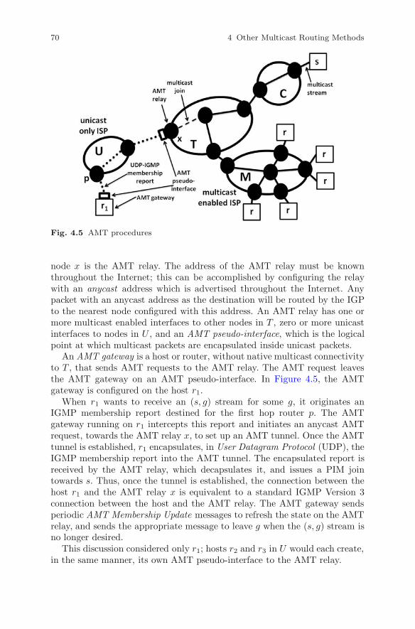
70 4 Other Multicast Routing Methods
Fig. 4.5 AMT procedures
node x is the AMT relay. The address of the AMT relay must be knownthroughout the Internet; this can be accomplished by configuring the relaywith an anycast address which is advertised throughout the Internet. Anypacket with an anycast address as the destination will be routed by the IGPto the nearest node configured with this address. An AMT relay has one ormore multicast enabled interfaces to other nodes in T , zero or more unicastinterfaces to nodes in U , and an AMT pseudo-interface, which is the logicalpoint at which multicast packets are encapsulated inside unicast packets.
An AMT gateway is a host or router, without native multicast connectivityto T , that sends AMT requests to the AMT relay. The AMT request leavesthe AMT gateway on an AMT pseudo-interface. In Figure 4.5, the AMTgateway is configured on the host r1.
When r1 wants to receive an (s, g) stream for some g, it originates anIGMP membership report destined for the first hop router p. The AMTgateway running on r1 intercepts this report and initiates an anycast AMTrequest, towards the AMT relay x, to set up an AMT tunnel. Once the AMTtunnel is established, r1 encapsulates, in User Datagram Protocol (UDP), theIGMP membership report into the AMT tunnel. The encapsulated report isreceived by the AMT relay, which decapsulates it, and issues a PIM jointowards s. Thus, once the tunnel is established, the connection between thehost r1 and the AMT relay x is equivalent to a standard IGMP Version 3connection between the host and the AMT relay. The AMT gateway sendsperiodic AMT Membership Update messages to refresh the state on the AMTrelay, and sends the appropriate message to leave g when the (s, g) stream isno longer desired.
This discussion considered only r1; hosts r2 and r3 in U would each create,in the same manner, its own AMT pseudo-interface to the AMT relay.

4.5 Distributed Delay Constrained Multicast Routing 71
4.5 Distributed Delay Constrained Multicast Routing
Sometimes, e.g., for audio or video streams, the total delay from a sourcenode s to a receiver node t cannot exceed a specified bound Δ. Suppose theproblem is to compute a least cost path from s to t subject to this delayconstraint. A path is feasible if the total delay on the path does not exceedthe bound. For such constrained routes, the next hop from some node n willin general depend on the set of arcs traversed from s to n. This is illustratedin Figure 4.6. Associated with each arc is the pair (c, d), where c is the cost
Fig. 4.6 Delay constrained routing
and d is the delay. Suppose Δ = 12, and consider a packet arriving at Cdestined for T . If the source is A, then the minimum cost path A−C−D−Tis not feasible, since its delay is 15, so C must send the packet to E; the costof path A − C − E − T is 10 and the delay is 7. If the source is B, thenC should send the packet to D; the cost of path B − C − D − T is 8, andthe delay is 11. Thus, in this example of constraint based routing, the nexthop at C depends on the path taken by the packet prior to reaching C. Forshortest path routing, in the absence of any constraints the next hop froma given node depends only on the destination of the packet, and not on thepath taken by the packet prior to reaching the node.
Delay is just one quality of service (QoS) constraint. QoS constraints canbe additive (summed over all links in a path), e.g., delay, cost, and jitter,or min/max (where the min/max is taken over all links in a path), e.g.,bandwidth. For min/max constraints, any link not providing the requiredresource can simply be pruned from the network, so we assume this has beendone, and consider only additive constraints. Both centralized and distributedheuristic methods have been proposed to solve, or approximately solve, theproblem of computing a minimum cost path subject to one or more additiveconstraints; many are described by Ben Ali, Belghith, Moulierac, and Molnar[13]. One approach to this problem is to compute, for each receiver node, aconstrained shortest path from the source node to the receiver node. Theunion of these paths forms a subgraph which in general must be pruned to

72 4 Other Multicast Routing Methods
eliminate cycles without violating the constraints. Greedy and taboo searchprocedures for pruning have been proposed [13].
Jia [54] proposed in 1998 a tree based method for multicast routing froma single source node to multiple receiver nodes, subject to a single additiveconstraint. The given data is an undirected graph (N ,A), the cost cij anddelay dij of arc (i, j) ∈ A, a source node s ∈ N , and a set of receiver nodesD ⊆ N . For t ∈ D, let P (s, t) be the unique path from s to t in a tree.Then the delay constraint is
∑(i,j)∈P(s,t) dij ≤ Δ for t ∈ D. The problem is
to construct a tree T , rooted at s and connecting to each t ∈ D, such thatthe tree cost is minimized subject to the delay constraint. For brevity, by ashortest path we mean a minimal cost path.
Jia’s method assumes that each node stores the minimal cost to eachother node (and a corresponding shortest path), and also the delay of theshortest path computed. Two assumptions are required. The first assumptionis that, for any two arcs a1 and a2, if c(a1) ≥ c(a2) then d(a1) ≥ d(a2).Under this strong assumption, the shortest path between any two nodes isalso the least delay path between the two nodes. For t ∈ D, let P�
d (s, t) beminimal delay path from s to t. The second assumption is that for t ∈ D wehave
∑a∈P�
d(s,t) da ≤ Δ. This assumption guarantees the existence of a tree
satisfying the delay constraint.In Jia’s distributed method, each node operates independently, executes
exactly the same algorithm, using only local information, and each nodeexchanges routing updates with neighboring nodes. The method starts byinitializing T = {s} (i.e., initially T contains just the source node, and noarcs) and then growing T . If node t is not in T , by a shortest path from t toT we mean a path P (t, n), using arcs in A, such that n ∈ T and the cost ofthis path does not exceed the cost of any other path from t to a node in T .If P (t, n) is a shortest path from t to T , we call n the tree node closest to t.
The method can be summarized as follows. Starting with T = {s}, we pickthe node t1 ∈ D that is closest to s; the shortest path from t1 to s is addedto T . We then pick the node t2 ∈ D such that t2 is not in T and t2 is closestto T under the delay constraint; we add to T the shortest path from t2 tothe tree node closest to t2. This process continues, where at each iterationwe pick the node t not in T which is closest to T under the delay constraint,and then add to T the shortest path from t to the tree node closest to t.This continues until all nodes in D have been added to T . It is proved in [54]that this method generates a tree spanning the nodes of D and satisfying thedelay constraint.
The method uses three data structures. The structure T2D (tree to desti-nation), with global scope, has 3 fields: for t ∈ D, the field T2D[t].cost is thecost from T to t, the field T2D[t].treenode is the tree node closest to t, andT2D[t].inTree is 1 if t ∈ T and 0 otherwise. Second, for t ∈ T , node t storesdelay[t], the total accumulated delay in the path in T from s to t. Finally,each node n maintains a routing table RTn, where if u ∈ N , then RTn[u].cost

4.5 Distributed Delay Constrained Multicast Routing 73
is the cost of the shortest (unicast) path from n to u, and RTn[u].delay isthe delay of that shortest path to u.
By D−{s} we mean the set {t | t ∈ D, t �= s}. The source node s does thefollowing:(i) For t ∈ D − {s}, initialize T2D[t].treenode = s and T2D[t].inTree = 0(since s is the only node in T ), and initialize T2D[t].cost to the cost of theshortest path from s to t.(ii) Let t1 ∈ D be any node such that t1 is closest to T . Add t1, and all thearcs on the shortest path from s to t1, to T .(iii) Let v be the successor node to s on the shortest path from s to t1. Setdelay[v] = RTs[v].delay (the delay from s to v on this shortest path).(iv) Send a setup message from s to v with the parameters delay[v], T2D,and D.
Let D − T be the set of nodes in D but not in the tree T . Now considera node v receiving a setup message. Upon receiving the message, v does thefollowing:(v) Determine, for each t ∈ D − T , if (a) RTv[t].cost < T2D[t].cost (i.e., ifthe cost from v to t is less than the cost from the current T to t), and also if(b) delay[v] + RTv[t].delay ≤ Δ (i.e., if the delay from s to v, plus the delayfrom v to t, is less than the bound Δ).(vi) If both (a) and (b) are true for some t ∈ D − T , then the path from sto this t through v is a feasible and shorter path than the current path, so vmakes the updates T2D[t].cost = RTv[t].cost and T2D[t].treenode = v (theclosest node in T to t is v).(vii) Node v sends a setup message to the next node, say w, on the shortestpath from s to t1. The parameters of the setup message are delay[w] =delay[v] + RTv[w].delay (the delay from s to v plus the delay from v to w),T2D, and D.
Steps (v)-(vii) continue until t1 has been reached and has executed steps(v)-(vii). At this point:(viii) Pick as the next receiver node t2 the node in D − T which is closestto T , i.e., the node t in D − T for which T2D[t].cost is smallest. Let z =T2D[t2].treenode (the node in T closest to t2). Note that, in general, z is afork node, meaning that there are more than two arcs in T incident to z.Add to T the path from t2 to z.(ix) Send a fork message to z, instructing z to send a setup message to thenext node on the shortest path from z to t2, with parameters delay[f ], T2D,and D. Continue as before, sending setup messages along the shortest pathfrom z to t2, until finally t2 has been reached and has executed steps (v)-(vii).Then select t3 as the node in D − T which is closest to T , and continue inthis manner until all nodes in D have been added to T .
We illustrate the method using Figure 4.7 and with Δ = 13. Next toeach arc (i, j) is the arc cost cij . To simplify the exposition, assume thatdij = cij for all (i, j) ∈ A; the algorithm of [54] allows cij and dij to bespecified independently. There are three receiver nodes, c, g, and p. We ini-

74 4 Other Multicast Routing Methods
tialize T = {s}. (i) At s we initialize T2D[p].cost = 5, T2D[p].treeNode = s,
Fig. 4.7 Delay constrained tree
T2D[p].inTree = 0, T2D[c].cost = 7, T2D[c].treeNode = s, T2D[c].inTree =0, and T2D[g].cost = 12, T2D[g].treeNode = s, T2D[g].inTree = 0. Sincethe cost to p is lowest, the shortest path from s to p is added to T , and ssends a setup message towards p. Since f is the next node on the shortestpath from s to p, and at s we have RTs[f ].delay = 2, we set delay[f ] = 2 andinclude delay[f ], T2D, and D in the setup message to f .
Node f determines that for t = c and t = g we have RTf [t].cost <T2D[t].cost and delay[f ] + RTf [t].delay ≤ Δ, and thus f makes the updatesT2D[t].cost = RTf [t].cost and T2D[t].treenode = f for t = c and t = g.Specifically, f sets T2D[c].cost = 6 and T2D[g].cost = 11. The next node onthe path from f to p is p itself. The receiver nodes c and g are not yet in T ,and p determines that delay[p] + RTp[c].delay = 5 + 9 > Δ, so no update toT2D is made for c by p. Similarly, delay[p] + RTp[g].delay = 5 + 10 > Δ, sono update to T2D is made for g by p.
Since T2D[c].cost < T2D[g].cost (i.e., 6 < 11), c is selected as the nextreceiver node. For c we have T2D[c].treeNode = f , so f is a branching node.The shortest path from c to f is added to T . Now a fork message is sent to f ,which sends a setup message to e, the next node on the shortest path from fto c. Node e determines that for g (the only receiver node not yet in T ), wehave RTe[g].cost < T2D[g].cost (i.e., 7 < 11) and delay[e]+RTe[g].delay < Δ(i.e., 6 + 7 ≤ Δ). So e sets T2D[g].cost = 7 and T2D[g].treenode = e. Thenext node on the shortest path from e to c is c itself, and c determines thatRTc[g].cost < T2D[g].cost (i.e., 5 < 7) and delay[c] + RTc[g].delay < Δ (i.e.,8 + 5 ≤ Δ) so c sets T2D[g].cost = 5 and T2D[g].treenode = c.
Now g is selected at the final receiver node, and the shortest path from cto g is added to T . Since all nodes in D have been added to the tree, we aredone.

4.6 Ant-Based Method for Wireless MANETs 75
Huang and Lee [51] discovered that the network generated by Jia’s methodcan contain cycles, and showed that with additional cycle processing andtree pruning steps, the modified method is (under Jia’s two assumptions)guaranteed to produce a tree satisfying the delay constraint.
4.6 Ant-Based Method for Wireless MANETs
The 2008 method of Shen, Li, Jaikaeo, and Sridhara [99] utilizes swarmintelligence techniques in a distributed heuristic for dynamically building adelay constrained Steiner tree that minimizes the total transmission powerin a wireless network. Let (N ,A) be an undirected wireless network, wherethere is an arc a ∈ A between two nodes if they have sufficient power to com-municate with each other. Since a wireless node broadcasts packets whichcan be received by any node within a radius determined by the transmissionpower (as opposed to wired networks which must duplicate packets on out-going interfaces), the cost and delay functions in the problem formulationare defined over the set of nodes, not the set of arcs. The cost of each nodedepends on the transmission power assigned by the method to the node. Ifnode i forwards packets to j, then i must have power at least rij which de-pends on various parameters, including the distance between i and j. If iforwards packets to all nodes in some set J , then i must have power at leastmaxj∈Jrij.
Let cp(n) be the cost of node n when its power assignment is p. Let d(n)be the transmission delay associated with using node n; the delay d(n) isassumed to be independent of the power assigned to n (this will be true, e.g.,if delay measures hop count). Let s be the source node, and let D ⊆ N −{s}be the set of receiver nodes. A forwarding set F ⊂ N is a set of nodes thatprovide a path from s to all the receiver nodes; the forwarding set includess and may include receiver nodes which also act as forwarders. Since thereare no physical arcs, each t ∈ D joins a unique forwarding node, which inturn joins another forwarding node, until the join reaches s. The problem isto determine a forwarding set F , and a power assignment to each node in F ,that minimizes the objective function
∑n∈F cp(n), The tree must also satisfy
the constraint that the delay from s to each t ∈ D cannot exceed Δ, for somespecified bound Δ.
The tree T is initialized when each t ∈ D computes a shortest path tos, where the cost of arc (i, j) ∈ A is proportional to the transmission powerrequired for nodes i and j to communicate. Associated with each forward-ing node n in T is the number height(n), which is defined as the highestnode identifier of the branch of T rooted at n, and where height(s) = ∞by definition. Once T is initialized, the method determines if these short-est paths can be merged by incorporating more forwarding nodes with lower

76 4 Other Multicast Routing Methods
power assignments. Employing the swarming idea, each receiver node peri-odically originates forward ant control messages. Two types of forward antmessages are used: (i) deterministic messages that are sent to the adjacentnode n for which the pheromone intensity (node desirability) is highest, and(ii) random ants, which explore other paths. Suppose the forward ant mes-sage from receiver node t reaches a forwarding node n on the tree for whichheight(n) > height(t). If the total delay from s to t via n does not exceed Δ,then the forward ant becomes a backward ant and returns to t, while increas-ing the pheromone intensity of nodes along the way, in order to attract joinrequests to the new path. The requirement height(n) > height(t) preventsa race condition in which receiver nodes attempt to merge onto each other’sforwarding paths and end up disconnected from the source.
Receiver t then recomputes its next hop by issuing a join to the neighbor-ing node x whose pheromone intensity is highest. The pheromone intensitiesdecay over time, so that changing network information (e.g., a node failure)will be reflected in new intensities. In turn, node x issues its own join, andthis process continues until the join reaches the source. This is illustrated inFigure 4.8. The initial forwarding set is F = {S, A, B, C, E}. When a for-
Fig. 4.8 Ant based routing
ward ant from D encounters N , it does not turn into a backward ant sinceN �∈ F . When it encounters C ∈ F , it does not turn into a backward antsince height(C) < height(D). When it encounters E, if the delay from D toS via E does not exceed Δ, it does turn into a backward ant, and increasesthe pheromone intensity of nodes E, C, and N .

Chapter 5
Inter-domain and Two-level Multicast
The scope (region of applicability) of an Interior Gateway Protocol (IGP),such as OSPF or ISIS, is a domain. The scope often corresponds to an AS,or it might be defined by the need to keep the number of nodes within thescale supported by the IGP protocol. An Exterior Gateway Protocol, typicallyBGP, interconnects two or more domains. Inter-domain multicast is requiredby an ISP, and is also required by a service provider whose customers spanmore than one IGP domain. In particular, when the set of source and receivernodes for a multicast group spans more than one domain, inter-domain mul-ticast routing is required.
Inter-domain multicast has two problems to solve. The first problem ishow to reach a source that is in a different domain than a receiver, and thedesired unicast and multicast topologies are not identical. This motivates thediscussion of MP-BGP in Section 5.1 below.
The second problem is how to connect PIM-SM domains served by differentRPs. For example, consider the case of two ISPs, each with its own AS. PIM-SM by itself does not allow more than one active RP for a given multicastgroup g. So if receivers in both ASs want to join g, the two ISPs must agree onwhose RP will be used. In practice, such collaboration is unrealistic, since eachISP wants administrative control of its own RPs. MSDP solves this problem,by letting nodes in each domain know about active multicast sources in theother domain (MSDP was introduced in Section 3.8.4 on Anycast RP). Thismotivates the discussion of MSDP in Section 5.2 below.
Noting that inter-domain multicast is a kind of two-level routing (within adomain at the lower level, and between domains at the higher level), we alsoexamine two other methods for two-level multicast routing: a method basedon the Yao graph and DVMRP.
5.1 Multiprotocol BGP
BGP [102] is the de facto standard for inter-domain routing. It is used,e.g., by ISPs to peer (inter-operate) with other service providers, and alsoby service providers who administer more than one AS. Multiprotocol BGP(MP-BGP) is required when a multicast group spans multiple ASs, and whenthe desired multicast topology differs from the unicast topology. (MP-BGPcan also be used inside a single AS when the desired unicast and multicast
E. Rosenberg, A Primer of Multicast Routing, SpringerBriefs in Computer Science, DOI 10.1007/978-1-4614-1873-3_5, © The Author 2012
77

78 5 Inter-domain and Two-level Multicast
topologies differ.) MP-BGP was defined in 2000 by IETF RFC 2283, andupdated in 2011 as an IETF proposed standard [11].
MP-BGP can distinguish between unicast routing and multicast routingby means of the MP REACH NLRI field in an MP-BGP message, whereNLRI means Network Layer Reachability Information. The NLRI field for areachable destination (e.g., a host or subnet) is the IP address prefix for thedestination. For example, the NLRI for a subnet might be 10.2.8.0/22. WithMP-BGP, BGP can provide both a unicast routing table and a multicastrouting table. MP-BGP does not itself build multicast trees; rather, it isused to exchange routing information used by other protocols, such as PIM,to build trees and forward multicast traffic.
To distinguish between different address families, MP-BGP uses an Ad-dress Family Identifier (AFI). For example, AFI 1 is for IPv4 and AFI 2 is forIPv6. Within each AFI are sub-AFIs. For example, within AFI 1, informationexchanged for multicast RPF calculations has sub-AFI 2.
Figure 5.1, adapted from [112], illustrates the use of MP-BGP. Router B,
Fig. 5.1 MP-BGP
in AS 456, has a single BGP session with router A in AS 123. Over this singleBGP session, B advertises to A that the subnet 192.10.8/24 is reachable inAS 456, and to reach this address, A should send packets to the BGP nexthop of 192.3.10.1. Over the same BGP session, B uses MP REACH NLRIwith AFI=1 and sub-AFI=2 to advertise the multicast source 192.10.8/24,but the BGP next hop is now 192.3.20.2. This means that if A sends a PIMjoin to B (so that A can receive this multicast stream), then the PIM joinfrom A must be sent to 192.3.20.2, and not to 192.3.10.1.
MP-BGP can be used in conjunction with SSM (Section 3.7.4) to buildinter-domain multicast trees. Suppose a host subtending node n wants toreceive the (s, g) stream, and g is in the SSM address range. Then the hostsends an IGMP Version 3 membership report to n, and then n sends a PIMjoin towards s. When a PIM join needs to cross from domain X to domainY , the MP REACH NLRI information tells a border node of X the address

5.2 Multicast Source Distribution Protocol 79
in Y to which the join should be sent. (A border node of a domain is a nodein that domain that is directly connected to a node in a different domain.)
5.2 Multicast Source Distribution Protocol
Multicast Source Distribution Protocol (MSDP) was developed so thatISPs exchanging multicast could peer with each other. It is also used byservice providers whose multicast networks span more than one domain. Con-sider a set of domains (ASs), each using PIM-SM as the multicast protocol.We allow the possibility that a domain might utilize multiple RPs, e.g., ifanycast RP is used. To implement MSDP, we first require MSDP peeringsessions to be established between pairs of RPs, between RPs and AS bor-der routers, and possibly between redundant RPs serving the same multicastgroups. There must be sufficiently many peering sessions to create a path ofsuch sessions between any two RPs in different ASs. When a set of MSDPpeers is fully meshed (i.e., each pair of RPs is linked by an MSDP session),the set is called a mesh group. For example, in Figure 5.2, the RPs do notform a mesh group, but there is a path of MSDP peers between any two RPs.
Fig. 5.2 MSDP
Suppose an RP in a domain learns, through the standard PIM mechanisms,of a source host s in that domain for group g. Then the RP encapsulates thefirst data packet from s for g in a source active (SA) message, which containsthe identity of the source domain. What happens next depends if the RP ispart of a mesh group. If it is, then the SA message is sent to all other membersof the mesh group. These other members do not resend the message withinthis mesh group, but do send the message to any other MSDP peers which

80 5 Inter-domain and Two-level Multicast
are not members of the mesh group. If the RP is not part of a mesh group,the SA message is sent to all the MSDP peers of the RP.
To prevent looping of MSDP messages, a modified RPF check is used byany node receiving an SA message. Consider a node n which receives, fromnode x, an SA message that originated from a source host s behind node y.A set of six rules [59] determine the peer-RPF neighbor of n (i.e., the MSDPpeer on the path from n towards the source), and whether n will accept ordrop the message. These rules are applied in order, and the first rule thatapplies is used. One rule has already been noted: if n and x are in the samemesh group, then n accepts the message from x. (Thus using a mesh groupreduces SA flooding and simplifies the peer-RPF check.) Another rule is thatif x = y, the message is accepted (i.e., accept the message if it is directlyreceived from the source node). The last rule we mention applies to the casewhere n and y are in different ASs, where n and x and are in the same AS,and x is an autonomous system border router, i.e., a node in one AS directlyconnected to a node in another AS. If x is the BGP next hop from n to y(i.e., if n learned about y from x), then x is the peer-RPF neighbor, and itsSA messages are accepted by n.
We illustrate this using Figure 5.2. Assume that BGP routing has deter-mined the best path from D1 and D5 to the source domain D4 is a directpath (traversing no via domains), the best path from D2 to D4 is via D1,and the best path from D3 to D4 is via D5. Suppose RP4 learns of the sourcein Domain 4 for group g. Then RP4 sends an SA message to its peers RP1,RP5, and RP6, who accept the message, since it was originated by the send-ing RP. RP6 has no other MSDP peers, so it does not forward the message.RP1 will send the SA message to its peers RP2 and RP3. RP2 will acceptthe SA message, since the best path from D2 to D4 is via D1. However, RP3
will discard the SA message, since its best path to D4 is via D5, and none ofthe other RPF rules will cause RP3 to accept the message. RP2 forwards themessage to RP3, which discards it. RP5 forwards the message to RP3, whichaccepts it, since the best path from D3 to D4 is via D5. RP3 forwards themessage to RP1 and RP2, which discard it.
Returning to the general case, suppose RP n, in domain Dn, receives anSA message about a source host s subtending the source node n(s) in anotherdomain Ds for group g, and the RPF check passes. If n has no (�, g) state,then no receiver host in domain Dn joined g, and hence there is no shared treefor (�, g) rooted at n. If n has (�, g) state, then some receiver host interestedin g has joined to n, so n creates (s, g) state and sends an (s, g) join towardss, in order to join the shortest path tree rooted at n(s). Note that this treewill in general span multiple domains, and therefore both intra-domain andinter-domain protocols (e.g., OSPF and MP-BGP) may be required for thisjoin. If n has (�, g) state, then n must also ensure that hosts in its domainDn know of (s, g). So n decapsulates the SA message and sends the packetdown the (�, g) shared tree in Dn rooted at n.

5.2 Multicast Source Distribution Protocol 81
When a last hop router (the router on the tree that is closest to somereceiver host) receives the decapsulated packet, it may itself join the (s, g)shortest path tree rooted at n(s). For example, referring to Figure 5.3, sup-pose host r subtending the last hop router z in D3 has joined RP3 to receive g.Then the (s, g) stream, if its bandwidth does not exceed the SPT-threshold,
Fig. 5.3 SPT join with MSDP
will take the path s → n(s) → RP4 → RP5 → RP3, and then down theshared tree rooted at RP3 to r, as illustrated by the solid lines. If the band-width of the stream does exceed the SPT-threshold, node z will directly jointhe (s, g) shortest path tree rooted at n(s), so the (s, g) stream takes the paths → n(s) → A → B → z → r, as illustrated by the dotted lines.
MSDP allows load sharing by multiple RPs within a given PIM-SM mul-ticast domain; this technique is called anycast RP, which was introduced inSection 3.8.4. Consider Figure 5.4. There are three RPs. With anycast RP,
Fig. 5.4 Anycast RP

82 5 Inter-domain and Two-level Multicast
we give the same unicast address to each of the RPs. Since a node uses uni-cast routing to send a PIM join or register message to the RP, a PIM join orregister from n1 will reach only RP1, since it is closer to n1 than is RP2 orRP3. Similarly, a join or PIM register from n2 will reach only RP2, since itis closer to n2 than is RP1 or RP3.
Referring again to Figure 5.4, consider a source host s1, behind n1, forgroup g. At RP1, the first packet in the (s1, g) stream will be encapsulatedin an SA message, and sent over MSDP sessions to RP2 and RP3, where it isdecapsulated and sent to any receiver nodes in the shared trees rooted at RP2
and RP3. Similarly, consider a source host s2, behind n2, for group g. At RP2,the first packet in the (s2, g) stream will be encapsulated in SA messages, andsent over MSDP sessions to RP1 and RP3, where it is decapsulated and sentto any receiver nodes in the shared trees rooted at RP1 and RP3. Thus, ingeneral, the set of anycast RPs share the work required of an RP. If RP1
fails, then normal IP unicast routing will determine a path to either RP2
or RP3 (provided such a path exists) and these other RPs will share theresponsibilities of RP1. Similarly, if some arc on the shortest path from n1 toRP1 fails, IP routing will determine either another path to RP1 or a path toa different RP, whichever has lower cost.
5.3 Two-level Routing using the Yao Graph
A two-level multicast routing method was proposed in 2008 by Lua, Zhou,Crowcroft, and Van Mieghem [67]. The multicast domain is subdivided intoclusters. Within each cluster are the level-0 (lowest level) peer nodes and oneor more level-1 super-peer nodes. Each peer is connected to its closest super-peer. The super-peer logical connectivity is established using the Yao graph[114] to partition two-dimensional Euclidean space R2. For a fixed positiveinteger k (k = 6 is used in [67]) and for each super-peer n, the space aroundn is partitioned into k sectors, where each sector is an unbounded cone withangle 2π/k and with n as a vertex. For i = 1, 2, · · · , k, let zi(n) be that super-peer in sector i that is closest to n. The undirected arc (n, zi(n)) becomes anarc in the super-peer graph. Thus each super-peer is connected to at most kother super-peers (some sectors may contain no super-peers other than n).This is illustrated in Figure 5.5 which for k = 6 shows the nodes to whichnode n is connected. In Sectors 1-5, node n is connected to that node in thesector closest to n. In Sector 6, there are no nodes other than n. This figureshows only the arcs emanating from n. To build the Yao graph, the sameprocedure is executed for each super-peer in the graph. The advantage of theYao graph for mobile or ad hoc networks is that it uses only local informationand is easily updated when there is network churn (e.g., nodes fail).
Routing at the level-1 super-peers layer uses local compass routing, in whicha node n selects the next hop based only on the destination d and the nodes

5.4 Two-level Routing using DVMRP 83
Fig. 5.5 Yao graph
in the Yao graph adjacent to n. For each node x adjacent to n in the Yaograph, the angle � xnd is computed, and the x yielding the smallest angleis chosen as the next hop. A variant of this scheme is random local compassrouting, in which x1 is chosen to be node above the line through n and dwhich minimizes the angle � x1nd, and x2 is chosen to be node below the linethrough n and d which minimizes the angle � x2nd; then n randomly choosesx1 or x2 as the next hop.
Inter-cluster routing (at the super-peers level) from source node s is ac-complished by building source trees. When a source peer node s wants tosend a packet to group g, it sends the packet (using unicast routing) to theclosest super-peer n(s); the super-peer n(s) must also join g if it has notalready done so. A super-peer n receiving a packet for group g does an RPFcheck to see if the packet arrived on the arc that n would use to route tos; if the check passes, the packet is forwarded on all links from n to othersuper-peers. Pruning can be used to remove branches of the tree with nodownstream group members.
5.4 Two-level Routing using DVMRP
Thyagarajan and Deering [106] proposed in 1995 a method that partitionsa multicast domain into regions. A unique region identifier (ID) is assignedto each region. Each region contains level-1 (L1) nodes responsible for for-warding multicast traffic within a region; each L1 node belongs to a singleregion. Level-2 (L2) boundary nodes are used to forward traffic between re-gions; an L2 node connecting regions A and B also provides L1 functionalityto regions A and B. This is illustrated in Figure 5.6, where there are two L1nodes in Region A, two in Region B, four in C, and one in D. One L2 node

84 5 Inter-domain and Two-level Multicast
Fig. 5.6 Level 1 and level 2 routers
interconnects Regions A and B, one interconnects A and D, two interconnectB and C, and two interconnect C and D, where each L2 node also providesL1 functionality in the two regions it interconnects.
The L1 nodes in a region are assumed to run the same standard multicastprotocol (which, at the time of this proposal, included DVMRP and MOSPF).Different regions may run different intra-region protocols. Consider a packetfor group g originated in a given region R. The intra-region protocol is usedto forward the packet to all receiver nodes for g in R, and, by default, to allthe L2 nodes attached to R.
The L2 nodes perform L2 inter-region routing using DVMRP, which cre-ates a tree for g, spanning all the regions, and rooted at the source node inthe source region (the source node, for this computation, is treated as an L2node). For example, suppose in Figure 5.7 that there are receiver hosts for gin Region C subtending the L1 nodes L1c, L1d, L1e, and L1f . Suppose theDVMRP tree is given by the heavy solid lines (which represent a path in aregion, and not necessarily a single link). There are three L2 nodes attachedto Region C used in the L2 tree: L2a, L2b, and L2d. Each of the four nodesL1 nodes in Region C must determine from which of those three L2 nodesthey will receive packets for g. To accomplish this, each L2 node floods withinits two attached domains a default cost. Using these default costs, each L1node determines the closest attached L2 node. This yields, in each region,a partition of the L1 nodes, with the L1 nodes in each partition forming asubtree rooted at an L2 node. For example, in Figure 5.7, in Region C thenodes L1c, L1d, and L1e are in the subtree rooted at L2a; the nodes L1f ,L1g, and L1h are in the subtree rooted at L2b; and the nodes L1w and L1xare in the subtree rooted at L2d (no L1 nodes in region C connect to L2c forthis g).

5.4 Two-level Routing using DVMRP 85
Fig. 5.7 Level 2 tree created by DVMRP
For each region R, all the L2 nodes attached (i.e., directly connected) toregion R form an L2 multicast group g(R); the number of L2 multicast groupsis thus equal to the number of regions. For an L2 multicast group g(R), asource is an L2 node attached to R, and the receivers are all the other L2nodes attached to R.
A Region Membership Report (RMR) is used to inform all L2 nodes at-tached to R about hosts in R interested in receiving traffic for g. An L1 nodex in R sends an RMR periodically, and upon triggered events, e.g., when thefirst host subtending x joins g, or when the last host subtending x leaves g.This is analogous to the use of IGMP by hosts to signal group membership.The L2 multicast group g(R) is used to distribute the RMR to all the L2nodes attached to R.
If an L2 node n attached to R learns through RMR reports that there areno receivers for g in R, then n issues a DVMRP prune to its upstream L2node. If sometime later a receiver for g does appear in R, then n can issue aDVMRP graft message for g to its upstream L2 node to get reconnected tothe tree for g.
Let R1(n) and R2(n) be the two regions connected by the L2 node n. Noden knows the ID of all the regions, and, by RMR reports, n also knows theaddresses of all the receiver hosts in the regions R1(n) and R2(n). When anL2 node n receives a non-encapsulated packet for g, the following happens.(i) Node n checks that the source of the packet is in one of its attachedregions R1(n) or R2(n); if not, the packet is discarded. Suppose, without lossof generality, that the source is in region R = R1(n).(ii) Node n encapsulates the packet with a tag specifying the source region,and with an outer label specifying the L2 node n, and the group g(R). Thepair (n, g(R)) is the (source, group) for the L2 multicast group. This is illus-trated in Figure 5.8.

86 5 Inter-domain and Two-level Multicast
Fig. 5.8 Level 2 encapsulation
(iii) The encapsulated packet is forwarded, by the L1 nodes, to all other L2nodes attached to region R.
When an L2 node n receives an encapsulated packet for g from an attachedregion, say R1(n), the following happens.(i) Node n decapsulates the packet and an RPF check is performed, usingthe originating region tag, to see if the packet arrived at n on the shortestpath to the source region; if not, the packet is discarded.(ii) If there are any receivers for g in the regions R1(n) or R2(n) attachedto n, then a copy of the original packet is injected into the region, where theL1 nodes in that region forward the packet to the receivers.(iii) Suppose there are regions downstream of n (i.e., downstream of n withrespect to the L2 inter-region tree created by DVMRP for this g) with re-ceivers. Such downstream regions can be identified using the source regiontag and the group address of the original packet. For each downstream regionwith receivers interested in g, the packet is forwarded across R2(n) to the L2nodes attached to R2(n) that are on the path to the downstream regions; atthese L2 nodes the above encapsulation process is applied.
This method can be extended to hierarchical multicast with h levels ofhierarchy (the above discussion assumed h = 2). For example, with h = 3, wecan cluster regions into super-regions interconnected by level-3 routers, andapply the encapsulating scheme recursively. Although this method was anearly advance in inter-domain multicast, it never enjoyed wide deployment,since MSDP became the method of choice to link multicast domains.

Chapter 6
Aggregate Multicast Trees
We have seen how a shared tree, e.g., as created by BiDir, reduces multicaststate by requiring only (�, g) state per node, rather than (s, g) state per nodefor a source tree. The subject of state reduction has enjoyed considerableattention, and various techniques, such as tunnelling, have been proposedto reduce state ([40], [74]). Even greater state reduction can be achieved byforcing multiple groups to use the same tree, in which case the tree is calledan aggregate tree. With aggregate trees, backbone nodes (with no subtendingsource or receiver hosts) need only keep state per aggregate tree, and not pergroup. Edge nodes (with subtending source or receiver hosts) still need tokeep state on a per group basis. Various approaches to aggregated multicastare described in [13] and [107].
Fei, Cui, Gerla, and Faloutsos [40] describe an aggregate tree scheme forinter-domain multicast. Referring to Figure 6.1, suppose Domain 1 is thebackbone network (interconnecting the backbone nodes) of an ISP, and theother domains attach to Domain 1. Consider first a group g1 with a source
Fig. 6.1 Tree aggregation
host in Domain 6, and receiver hosts in Domains 3, 4, and 5. The sharedtree for this group will impose (�, g1) state on the seven nodes B, C, D, E,F , G, H . Now consider a second group g2 that also has a source host inDomain 6, and receiver hosts in Domains 2, 4, and 5. The shared tree forthis group will impose (�, g2) state on the same set of seven nodes. Since
E. Rosenberg, A Primer of Multicast Routing, SpringerBriefs in Computer Science, DOI 10.1007/978-1-4614-1873-3_6, © The Author 2012
87

88 6 Aggregate Multicast Trees
within the backbone (Domain 1) the same multicast tree is used, we can usea single aggregate tree that spans these seven nodes. Thus, in Figure 6.1, forthe aggregate tree we must maintain one aggregate state on B, C, D, E, F ,G, H . However, we must still maintain per group state (g1 and g2) on theedge nodes B, C, and D; this is required in order for these nodes to correctlyroute packets to the receiver hosts. For example, B requires both g1 and g2
state in order to decide whether to send packets to Domain 2 or Domain 3.Thus we must carry per group (�, g) state on each packet as it traverses thebackbone, so that this information is available to the edge nodes. This stateis called irreducible since it must be maintained by edge nodes. One way toimplement such a scheme is to use MPLS, where an inner label carries (�, g)and the outer label identifies the aggregate tree.
Define the total state in the network (N ,A) as∑
n∈N state(n), wherestate(n) is the total number of aggregate and (�, g) states on node n. Usingthe method of [40], we can estimate the reduction in total state obtainedby using aggregate trees versus not using aggregation (i.e., using a distinctshared tree for each group). Let Sa be the total state using aggregate trees,and let S0 be the total state without aggregation. A simple measure of thestate reduction with aggregate trees is R = (S0 − Sa)/S0 = 1− Sa/S0. Sincesome of the state is irreducible, a better measure of the state reduction isobtained by letting Sir be the irreducible state, and defining
Rir =(S0 − Sir) − (Sa − Sir)
S0 − Sir= 1− Sa − Sir
S0 − Sir.
We have 0 ≤ Rir ≤ 1, and larger values of Rir mean more reduction instate by using an aggregate tree. For the example of Figure 6.1, withoutaggregation the trees in the backbone for g1 and g2 each require 7 states, soS0 = 14. With aggregation, Sir = 6, since 3 edge nodes are used by g1, and3 by g2. The aggregate tree requires 7 states. Hence Sa = 7 + (2)(3) = 13, soR = 1 − 13/14 = 1/14, and Rir = 1 − (13 − 6)/(14 − 6) = 1/8.
Let G be a set of multicast groups such that each g ∈ G uses the exactsame set of edge nodes, and let NE be the number of nodes in this set. (Ina large network, we can reasonably expect to find such a set.) Let the sameshared tree T be used for each g ∈ G, and let NT be the number of nodesin T . Assuming that the same procedure used to construct T is also used tobuild a shared tree for each g ∈ G, then each shared tree will also have NT
nodes.Using a distinct shared tree for each group, the total state S0 is given
by S0 = GNT , where G = |G|. Using one aggregate tree, the total stateis Sa = NT + GNE , since each of the NT nodes in the aggregate tree getsaggregate state, and each of the NE edge nodes gets (�, g) state for g ∈ G.Hence R = 1 − (NT + GNE)/GNT . Since the state for the G groups on theNE edge nodes is irreducible, we have

6.1 Leaky Aggregate Trees 89
Rir = 1 − (NT + GNE) − GNE
GNT − GNE= 1 − NT
G(NT − NE).
This expression quantifies the intuitive result that an aggregate tree is moreeffective when the number G of groups being aggregated is large, and thenumber NE of edge nodes used by each group is small compared to thenumber NT of nodes in the shared tree. For example, referring again to theabove example of Figure 6.1, suppose that, instead of just the two groups g1
and g2, we have G groups, where each of the G groups spans the same setof domains as g1. Then NE = 3 (three edge nodes in each group), NT = 7(seven nodes in the aggregate tree), S0 = 7G, and Sir = 3G. Thus R =1− (7 + 3G)/7G ≈ 4/7 for large G, and Rir = 1− 7/(7G− 3G) ≈ 1 for largeG, which indicates the efficiency possible with aggregation.
6.1 Leaky Aggregate Trees
Consider an aggregate tree T with node set NT , and consider a set G ofmulticast groups, where Ng is the set of receiver nodes used by g ∈ G. Wesay that T covers g if Ng ⊆ NT . If T covers g, then T can be used as ashared tree for group g. We do not allow T to be used for g if Ng �⊆ NT . IfNg is a proper subset of NT for some g, then leakage occurs, meaning thatbandwidth is wasted delivering traffic for g to a node behind which are nointerested hosts. For example, in Figure 6.1, if NT spans the edge nodes B,C and D but Ng spans only B and C, then leakage occurs since traffic isunnecessarily delivered to D. While leakage is undesirable, some leakage maybe acceptable in order to reduce multicast state.
Assume T covers g for g ∈ G. Let c(T ) be the cost of T , where, as usual,the cost of a tree is the sum of the arc costs over all arcs in the tree. LetTg be a tree spanning the receiver nodes of g. Defining G = |G|, the averageleakage L(T , G) incurred by using the aggregate tree T rather than the setof individual trees Tg, g ∈ G is defined in [40] as
L(T , G) =c(T ) − (1/G)
∑g∈G c(Tg)
(1/G)∑
g∈G c(Tg).
The larger L(T , G) is, the more bandwidth is wasted using T rather thanusing the group specific trees Tg for g ∈ G. This measure suggests a strategyto determine which groups to aggregate [40]. Let G be a set of multicast groupsfor which we are considering using one or more aggregate trees. Consider aset S which contains a set of aggregate trees that will be used to cover thegroups in G. For T ∈ S, let G(T ) be the set of groups in G which are coveredby the tree T . Initially, S = ∅. By extending a tree T to yield a new tree T ′

90 6 Aggregate Multicast Trees
we mean adding branches to T . Let δ be a given threshold parameter. Thestrategy is implemented in procedure Aggregate Trees() below.
procedure Aggregate Trees(G)1 initialize: S = ∅;2 for (g ∈ G) {3 for (T ∈ S) {4 if (T covers g and L(T ,G(T ) ∪ {g}) ≤ δ) set x(T , g) = 1;5 else set x(T , g) = 0;6 }7 if (x(T , g) = 0 for all T ∈ S), do either (i) or (ii) {8 (i) extend some T ∈ S to create a new tree T ′ covering g
such that L(T ′,G(T ) ∪ {g}) ≤ δ;9 set G(T ′) = G(T )∪ {g};10 (ii) set G(Tg) = {g} and add Tg to S ;11 }12 else {13 pick T � such that x(T �, g) = 1 and
c(T �) = min{c(T ) |x(T , g) = 1};14 set G(T �) = G(T �)∪ {g};15 }16 }
Fig. 6.2 Aggregate Trees()
A significant practical issue that must be addressed with an approach suchas procedure Aggregate Trees() is that group membership is dynamic, so anaggregate tree covering a group g may cease to cover g when new receiversjoin the group.
6.2 Hierarchical Aggregation
Let D be a multicast domain with node set N , and let Ng ⊆ N be theset of source or receiver nodes used by group g. If for some g1 and g2 wehave Ng1
= Ng2then the same shared tree can be used for g1 and g2. If the
members of g1 and g2 are chosen randomly, the probability that Ng1= Ng2
is small, and this probability decreases with the size of N . Therefore, if wedivide D into two subdomains, the likelihood of two groups using the sameset of nodes increases. With this motivation, Moulierac, Guitton, and Molnar[74] divide a domain into two or more subdomains, aggregate within eachsubdomain, and stitch the subdomains using tunnels.
A simple approach to dividing a domain is to first find the nodes n1 andn2 furthest apart; we initialize D1 = {n1} and D2 = {n2}. At each subse-

6.3 Aggregation of Forwarding State 91
quent iteration, the unassigned node nearest to D1 is assigned to D1 and theunassigned node nearest to D2 is assigned to D2. Subdomains can be furtherdivided, if desired.
Subdomain Di is controlled by a processor pi, which knows the topologyof Di and the groups with members in Di. Each subdomain contains one ormore border nodes, which are nodes that are directly connected to a node inanother subdomain. Suppose border node n ∈ Di receives, from some othersubdomain, a join request for g. Then pi adds n to the set of nodes used by gwithin Di, and decides whether to use an existing aggregate tree for g in Di
(e.g., if the bandwidth leakage does not exceed a given tolerance) or to builda new tree for g in Di.
A central processor p stitches together the subdomains for each group g.Each pi selects, for g, a border node bi(g) in its subdomain. Processor pi
informs processor p of the chosen bi(g), and p creates a set of unicast tunnelsto join these bi(g) nodes in a global tree for g. For example, suppose there are8 subdomains, but that g spans only Di, for i = 1, 3, 4, 6. Then p might createthe 3 bidirectional tunnels (b1(g), b3(g)), (b1(g), b4(g)), and (b1(g), b6(g)) toform a tree linking these 4 border nodes.
The method was simulated on a network with 201 routers and 10,000 mul-ticast groups. For simplicity, each pi(g) was chosen randomly from amongthe border nodes in subdomain i for g; more sophisticated schemes could bedevised. Define total state to be the sum of (i) the total router state in allthe routers and (ii) the state required for the inter-subdomain tunnels. Using4 subdomains, a 16% reduction in total state was achieved relative to 1 un-divided domain when no bandwidth leakage is allowed; with 20% bandwidthleakage allowed, the total state is reduced by 25%. Having 4 subdomains isalmost always better than having only 1 or 2.
6.3 Aggregation of Forwarding State
A standard technique in unicast routing is the use of a summary addressto represent a collection of more specific addresses. Since unicast addressesare often based upon geographical location, summary addresses can be cre-ated based on a geopolitical hierarchy [8], or a structured numbering plan[95]. For IP routing, variable length subnet masking (VLSM) [77] is used torepresent many subsets by a single address prefix. Because multicast groupaddresses are not tied to a geopolitical hierarchy, it is commonly believed thatmulticast state on a router cannot be aggregated. Thaler and Handley [104]demonstrate that multicast state in the forwarding table can be aggregated(so that less memory is consumed by the forwarding table), even when multi-cast addresses and group members are randomly distributed. They consider

92 6 Aggregate Multicast Trees
only perfect aggregation (as opposed to leaky aggregation), so that no trafficis needlessly sent to a node.
The basis of their aggregation scheme is a paradigm shift from the tradi-tional packet forwarding model (Section 1.5.1) that specifies, for each (�, g)or (s, g) entry, an RPF interface and an outgoing interface list (OIL). In thetraditional model, an incoming packet for (�, g) or (s, g) will be accepted onlyif it arrives on the specified RPF interface; if so, the packet is replicated andsent out on each interface in the OIL. The paradigm shift is to instead as-sociate with each interface an input filter and an output filter. For interfacei, Let F I
i be the input filter and F Oi be the output filter. A filter has the
output 1 (accept), 0 (reject), or “−” (don’t care). When a packet arrives oninterface i, it is dropped if F I
i = 0; otherwise, the output filter of each otherinterface on the node is checked to see if the packet should be replicated andsent out that interface.
While their model applies to source trees, which require (s, g) state, con-sider for simplicity the case of shared trees. We assume that a sparse modeprotocol like PIM-SM is run, so that a node n maintains (�, g) state onlyif there are receiver hosts for g downstream of n. Consider a particular in-terface i, and consider the input filter F I
i (this choice was arbitrary, andwe could have picked F O
i ). Let G be the address space, e.g., G is the set ofmulticast addresses from 224.0.0.0 to 239.255.255.255, and let G = |G| bethe size of the space. The crux of this method is to partition G into a setof regions. Referring to Figure 6.3, in region k, the addresses span the rangeak to ak+1 − 1, where F I
i (ak) = 1, and F Ii (ak+1 − 1) = 0. Each region is
Fig. 6.3 State aggregation
further divided into two sub-regions: for some bk such that F Ii (bk) = 1 and
F Ii (bk + 1) = 0 we have F I
i (g) = 1 or “−” for g ∈ [ak, bk], and F Ii (g) = 0 or
“−” for g ∈ [bk + 1, ak+1 − 1]. The demarcators ak and bk for subregion kdepend in general on the interface i and whether we are considering the inputor output filter for i. The significance of these two sub-regions of each regionis that the behavior of F I
i in the range [ak, ak+1 − 1] can be summarized bythe 3 demarcators ak, bk, and ak+1. It is in this sense that we have aggregatedthe state. If G is partitioned into K regions, then the behavior of F I
i (g) forg ∈ G is summarized by at most 3K demarcators. Therefore the objective isto have K as small as possible.
For simplicity of notation, we write F rather than F Ii . Assume that F is a
random variable defined on G, and the values {F (g) | g ∈ G} are independent.

6.3 Aggregation of Forwarding State 93
For g ∈ G, let p be the probability that F (g) = 1, let q be the probability thatF (g) = 0, and let r = 1− p− q (thus r is the “don’t care” probability). Thenthe expected number K of regions is approximately Gpq/(1 − r). The proofis as follows [104]. Define a success as the event that F (g) is either 1 or “−”;the probability of a success is 1 − q. The number of successes until a failurefollows a geometric distribution with probability q. The expected number ofsuccesses until a failure, which is the expected length of the “accept or don’tcare” sub-region in Figure 6.3, is
∑Gj=1 j(1 − q)jq. For large G, this sum is
approximated by∑∞
j=1 j(1− q)jq = (1− q)/q. Now re-define a success to bethe event that F (g) is either 0 or “−”; the probability of a success is now 1−p.The number of successes until a failure follows a geometric distribution withprobability p, and the expected number of successes until a failure, which isthe expected length of the “reject or don’t care” sub-region in Figure 6.3,is approximately
∑∞j=1 j(1 − p)jp = (1 − p)/p for large G. The expected
number of addresses that can be aggregated into a single region is therefore[(1− q)/q]+ [(1−p)/p] = (p+ q −2pq)/pq ≈ (p+ q)/pq = (1− r)/pq. Finally,since G = |G|, the expected number K of regions is approximately
K = G/[(1− r)/pq] = Gpq/(1− r) . (6.1)
Considering a given node n, define Gn to be the subset of G such that noden has (�, g) state for g ∈ Gn. Let Gn = |Gn|. We consider one application ofthe formula K = Gpq/(1− r) for input filters, and one application for outputfilters; more applications are discussed in [104]. A customer facing interfaceis an interface connected to a host, as opposed to an interface connected toanother node.
(i) Consider the input filter associated with some customer facing interface onnode n. Suppose the tree for each g is a bidirectional shared tree, and supposethe addresses g are uniformly distributed. Since no incoming interface check(i.e., no RPF check) is done, then p = Gn/G. Since also r = 0, then q = 1−pand (6.1) yields K = Gn[1− (Gn/G)] for this input filter. This expression ismaximized when Gn = G/2. If Gn << G, then K ≈ Gn, so no savings dueto aggregation has been achieved. However, Gn[1 − (Gn/G)] is a decreasingfunction of Gn for Gn > G/2, and K → 0 as Gn → G.
(ii) Consider the output filter associated with some interface i on node n.Suppose the addresses g are uniformly distributed, and suppose there are Jdownstream interfaces at n for each g. Suppose also that for each g there areM nodes downstream from n, and each of these M nodes is equally likely tojoin on one of the J downstream interfaces. Since all unused addresses are“don’t care,” then r = 1 − (Gn/G). The probability q that the output filtervalue for interface i is 0 for some g is the probability that g ∈ Gn and all Mdownstream nodes join on some interface other than i; thus q = (Gn/G)Q,where Q = [(J−1)/J ]M. Then p = 1−q−r = (Gn/G)(1−Q) and (6.1) yieldsK = GnQ(1 −Q). Since GnQ(1− Q) < GnQ and Q is a decreasing function

94 6 Aggregate Multicast Trees
of M , then K decreases as M increases. Hence aggregatability increases asthe average number of downstream members of a group increases.
6.4 Subtree Aggregation
We have shown how aggregate trees can be used, at the cost of some leak-age if the groups being aggregated do not span the same set of receiver nodes.Another approach is to search for a subtree that is common across the treesused by a set of multicast groups, and to replace the common subtrees by asingle aggregate subtree. Since only exactly the same subtrees are combined,there is no leakage with this method. As shown by Ciurea [26], this schemeis easily implemented with MPLS P2MP trees (Section 3.10). In order to im-plement subtree aggregation, we use downstream, on demand, ordered labelassignment [29]. Downstream assignment means that a downstream node ngenerates a label to be used by its parent node for any packet destined for n.On demand means that n generates a label only if n has received a request togenerate a label. Ordered means that label assignment proceeds in an orderlyfashion from one end of the LSP to the other.
Ciurea’s scheme is illustrated in Figure 6.4, where the receiver nodes forgroup x subtend nodes B, E, J , and L, and the receiver nodes for group ysubtend, at the outset, nodes C and E. Assume A, D, and H are backbonenodes, and all other nodes are edge nodes, at which all labels are imposedor removed. Suppose we start out with separate MPLS P2MP trees for x
Fig. 6.4 Initial configuration
and y. Assume we have the following rule: if the OILs at a node n for twogroups are identical, and if the upstream neighbor p of n is the same for bothgroups, then p can forward packets to n using the same label for both groups.Above each node in Figure 6.4 are the entries in the Multicast ForwardingInformation Base (MFIB) for groups x and y, e.g, if a group x packet isreceived by A with label 1, one copy is sent to B with label 2, and one

6.4 Subtree Aggregation 95
copy is sent to D with label 3. (With MPLS, labels are locally assigned, butfor clarity the figure uses globally unique labels. Also, in practice the MFIBwould specify the interface to an adjacent node, rather than just the nodeidentifier.) At H , if a group x packet is received with label 8, it is sent to Jwith label 9 and to L with label 10.
Now suppose a host behind J wants to join group y. Then J must tell itsparent H to send down packets for y. So J reuses the label 9 and tells H tosend group y packets to J with label 9. Node H must also tell its parent Dto send down packets for y. However, since at H the OILs for x and y are notidentical, H generates the new label 11 and tells D to send group y packetsto H with label 11. The updated MFIB entries at H and D for y are shownin Figure 6.5. Now suppose a host behind L wants to join group y. At this
Fig. 6.5 Host behind J joins group y
point, H recognizes that its OILs for x and y are identical, combines theminto a single OIL, and advertises the single label 8 to its upstream neighborD, as as shown above H in Figure 6.6. When D receives the message to send
Fig. 6.6 Host behind L joins group y
group y packets to H with label 8, D recognizes that its OILs for groupsx and y are now identical, and combines them into a single OIL, as shown

96 6 Aggregate Multicast Trees
above D in Figure 6.6. At A the two OILs are not identical, so they cannotbe combined.
Finally, suppose the host behind L leaves group y. Then H must disaggre-gate, and create separate MFIB entries for x and y, so the MFIB at H revertsto the one shown in Figure 6.5. Similarly, D must now disaggregate, and itsMFIB reverts to the one shown in Figure 6.5. For this reason, [26] suggeststhat each node store previously generated upstream label assignments.
In this example, when the host behind L leaves y, the label updates prop-agate only up to D. In general, with subnet aggregation, label updates forgroup g will propagate all the way to the root of the P2MP tree for g.

Chapter 7
Multicast Virtual Private Networks
When a customer (e.g, a business, university, or branch of government)needs secure and reliable telecommunications, it can build its own network,or it can go to a Service Provider (SP), such as AT&T, who offers VirtualPrivate Network (VPN) services over its backbone network. The adjectivevirtual reflects the fact that the customer does not have to manage a back-bone network, that the SP backbone routing procedures are transparent tothe customer, and that multiple customers can use the SP backbone withoutimpacting each other (if the SP backbone is properly engineered). A cus-tomer’s VPN may handle only unicast traffic, or may handle both unicastand multicast traffic; in the latter case, the VPN is called a multicast VPN(mVPN). Since multicast VPNs are an extension of unicast VPNs, we firstbriefly describe how unicast VPNs work. For brevity, we consider only Layer3 VPNs; see [49] for Layer 2 VPN methods.
7.1 Unicast VPNs
A VPN customer C pays for two or more interfaces in the SP backbonenetwork, and the VPN for C provides the ability to route IP packets betweenthe interfaces for C, just as if C had built its own dedicated network. Sincetypically each customer contracts with the SP for a single VPN, we willfor simplicity use customer and VPN synonymously, recognizing that somecustomers do order multiple VPNs from a given SP. Figure 7.1 illustrates aservice provider VPN architecture. Each host for C connects (not necessarilydirectly) to a customer edge (CE) router, typically owned and managed byC; for simplicity, in this figure only two CEs are shown. Each CE connectsto one or more provider edge (PE) routers, owned and managed by the SP.Many different CE routers, belonging to different customers, can connect to agiven PE. The PE routers have the responsibility for providing VPN features,such as the ability to provide different classes of service for different typesof customer traffic, and the ability to terminate different types of customerinterfaces (e.g., Ethernet or Packet over SONET). For simplicity, we assumeeach CE connects to a single PE. Each PE connects to one or more backbonerouters in the SP network. Service provider backbone routers are called Prouters. A PE router might connect only to the nearest P router, or it mightconnect to two P routers, e.g., to provide an alternate route if one of the PE-
E. Rosenberg, A Primer of Multicast Routing, SpringerBriefs in Computer Science, DOI 10.1007/978-1-4614-1873-3_7, © The Author 2012
97

98 7 Multicast Virtual Private Networks
Fig. 7.1 VPN architecture
P links fails. The P routers, typically running the IP and MPLS protocols,are workhorses designed to accept high speed interfaces and forward packetsto other P routers and to subtending PE routers. (In Figure 7.1, each of theP routers except P1 has a subtending PE.) The P routers handle many typesof SP traffic, e.g., VPN, Internet service, traditional wireline voice, or mobilevoice and data traffic. There are typically many more PEs than P routers inthe service provider network.
A VPN must satisfy three requirements: (i) Each customer has no accessto information on any other VPN customers supported by the SP. (ii) Eachcustomer must be allowed to use its own unicast or multicast address plan,regardless of the address plan used by other VPN customers supported bythe SP. (iii) Each customer has no access to information about PE routers towhich it is not attached, and no visibility into the SP backbone. In particular,each customer has no access to information about the P routers in the SPbackbone and about the SP’s internal addressing plan.
To meet these requirements, each PE stores a set of Virtual Routing andForwarding tables (VRFs). A PE will have a VRF for a given VPN if thereis a CE, belonging to that customer, which subtends the PE; in this case wesay that the PE is used by the VPN. Thus, if there are K PEs used by aVPN, each of the K PEs will have a VRF for this VPN. A VRF for VPN Vhas one forwarding table entry for each address prefix that is advertised by aCE for this customer to V . The information stored in a VRF on a given PE(call it X) for an address prefix p includes the cost to reach the PE (call itY ) that is advertising p, and the interface out of X on the best path to Y .
A VRF for a given VPN is populated as follows. Suppose CEp wantsto advertise an address prefix p throughout this VPN. Then CEp informs,typically using BGP, its local PE (call it PEp) about p. So PEp installs pin its VRF for this VPN. The service provider then distributes this addressprefix, using BGP, to the other PEs used by this VPN. Once p has beenreceived by some remote PE (call it PEx), p is installed in the VRF for this

7.1 Unicast VPNs 99
VPN on PEx. Then p is communicated, typically using BGP, to the CEs forthis customer that subtend PEx. If a CE for this customer subtending PEx
wants to send a packet to destination p, then the CE forwards the packet toPEx; the SP backbone network forwards it from PEx to PEp; finally PEp
forwards the packet to CEp.When the service provider forwards a customer packet from PEx to PEp,
the packet cannot be sent “natively” (i.e., unencapsulated) into the SP back-bone network, since the destination address in the customer packet refers toa customer address, and the SP backbone routers have no information aboutcustomer addresses. Therefore, a customer’s data packet is encapsulated tohide the customer destination address from the backbone routers. The en-capsulation must carry the information needed by the SP backbone networkto forward the packet from PEx to PEp.
Since each customer independently chooses its own addressing plan, differ-ent customers might use the same address prefix. For example, two customersmight both want to advertise the address prefix 10.1.2.0/24. BGP, used bythe SP to distribute address prefixes within a VPN, needs a way of unambigu-ously determining which address prefix is associated with which VPN. Thisis accomplished by associating with each VRF a unique identifier, known asa Route Distinguisher (RD). Consider an address prefix p installed in a VRFon some PE. Prepending the VRF RD to p yields a VPN-IP address, which iscustomer specific. For example, if VRF 1 has RD1 and VRF 2 has RD2, thenfor the address prefix 10.1.2.0/24, the VPN-IP addresses RD1 : 10.1.2.0/24and RD2 : 10.1.2.0/24 are now unique within the SP network.
Each VRF in a VPN is also associated with a set of import Route Targets(import RTs) and a set of export Route Targets (export RTs). When a PE usesBGP to advertise a particular VPN-IP address prefix from a particular VRF,it advertises the VRF’s export RTs as attributes (i.e., associated parameters)of the VPN-IP address prefix. A VRF imports (i.e., accepts) a given VPN-IP address prefix if the address prefix carries (as an attribute) a RT thatis one of the VRF’s import RTs. Typically, for a given VPN all VPN-IPaddresses prefixes are advertised with the same RT, and all VRFs for theVPN import that RT, so all VRFs learn all address prefixes for the VPN.Alternatively, RTs can provide fine grain control over which VRFs installwhich address prefixes. This is useful, e.g., in a hub and spoke topology inwhich spoke locations can talk only to hubs, but not to each other. RTs canalso be used to control the distribution of multicast state, as discussed inSection 7.4 below.
The mechanisms for distributing customer address prefixes, RDs, and RTsamong the PEs used by a VPN are called control plane procedures. Themechanisms for forwarding actual customer packets to the PEs used by aVPN are called data plane procedures. The service provider is responsible forimplementing both the control plane and data plane procedures. In the abovedescription of unicast VPNs, we have described the control plane proceduresfor distributing customer address prefixes. The data plane for unicast IP

100 7 Multicast Virtual Private Networks
VPNs is typically either native IP routing or MPLS forwarding, with tunnelsbetween PEs to hide customer address prefixes from backbone routers.
Thus far we have only defined unicast VRFs. We define a multicast VRF(mVRF) as the routing/forwarding table associated with (�, g) or (s, g) multi-cast state, for customer group g (where g is in the customer multicast addressspace) and customer source host s, for a given customer on a given PE. Theentry in a given mVRF on a PE corresponding to a given (�, g) or (s, g)state provides the RPF interface (towards the root of the customer shared orsource tree) and the outbound interface list (OIL) over which incoming pack-ets should be sent. Finally, a multicast VPN (mVPN) is a VPN which alsocontains a set of mVRFs with interfaces that can send multicast packets toeach other. A multicast packet, sourced by customer host s and for customermulticast group g, that is received by a PE is sent over the SP backbone net-work to one or more destination PEs, in order to reach the destination CEsfor that customer which have subtending receiver hosts interested in (�, g)or (s, g) packets. These destination PEs can be spread among the set of PEsused by the VPN.
We will discuss two current methods for implementing mVPNs: RFC 6037([93], see also [18], [83]) and a BGP based method ([3], [57], [58]). Theydiffer in their control plane mechanisms for distributing customer multicastinformation: in RFC 6037 the PE-PE multicast control plane uses PIM, whilein the BGP based method the PE-PE multicast control plane uses BGP.The BGP based method is a particular variant of the newer IETF standardmVPN scheme [91], which supports using either BGP or PIM for the PE-PEmulticast control plane.
7.2 Draft-Rosen
For convenience we refer to RFC 6037 as draft-Rosen, since it was originallydescribed in [92] and is well known by that name. The essence of the draft-Rosen method is that one multicast group is defined in the SP network foreach multicast customer. The set of source and receiver nodes used by thisgroup is precisely the set of PEs spanned by the customer mVPN. In the SPnetwork, the multicast traffic is carried by a default Multicast DistributionTree (default MDT), which is built using PIM-SM or SSM or BiDir. Thedefault MDT is built in the SP network by running an instance of PIM, onthe PE and P routers, that operates in the SP multicast address space (notin a customer multicast address space).
All multicast control traffic for this customer, as well as low bandwidthcustomer data traffic, is carried over the default MDT. For high bandwidthsources, a data MDT, typically created using SSM, can be used to send traf-

7.2 Draft-Rosen 101
fic only to PEs that have interested subtending receivers. We now describedefault MDTs and data MDTs in more detail.
7.2.1 Default MDT
Consider a given mVPN V . An mVRF for V is created on a PE by ap-propriate configuration of the PE, and this does not depend on having activemulticast source hosts or receiver hosts for V on any CE subtending the PE.If a PE has an mVRF for V , we say that the PE is used by V . Thus whetheror not a given PE is used by V is a static, rather than dynamic, condition.Let PEV be the set of PEs used by V . The Multicast Domain for V is the setof mVRFs for V (thus the terms multicast domain and multicast VPN aresynonymous).
The SP assigns to V a unique multicast group address in the SP multicastaddress space; we denote this address by GV . Previously we have exclusivelyused lower case g to refer to a multicast address; here we use G to emphasizethat this is a multicast address in the service provider address space, andGV is the service provider multicast address assigned to V . We will continueto use lower case g to refer to a multicast address in the customer multicastaddress space.
Regardless of the number of customer multicast groups supported in agiven mVPN V , the SP creates for V , using PIM, one default MDT. Thedefault MDT for V connects all |PEV | PEs in V through the SP backbonenetwork. No PE in PEV is allowed to be pruned from the default MDT for V .The default MDT can be created using any PIM technique preferred by theservice provider: PIM-SM, BiDir, or SSM. The default MDT for V is createdby running PIM on the PE and P routers in the SP network, using the addressGV . The address GV and the default MDT for the multicast customer V aretransparent to the customer. In order to use PIM-SM to create the defaultMDT for V , one or more RPs for the address GV must be deployed in theSP network. If there are multiple RPs for a given address GV , they can beinterconnected using MSDP.
A logical multicast tunnel interface (MTI) is defined on each mVRF for V .The MTI appears, to an mVRF, to be a LAN interface, and so each mVRFfor V views the other mVRFs for V as belonging to that LAN. Thus a PIMadjacency can be established between each pair of mVRFs for V , even thougheach adjacency is actually formed between two distinct PEs separated by oneor more P routers.
The default MDT for V delivers both customer control data packets (e.g.,customer multicast domain PIM joins and prunes) and customer multicastdata packets for V to each PE in PEV , whether or not there are interestedreceiver hosts behind these PEs. To distinguish between SP and customer

102 7 Multicast Virtual Private Networks
packets, we write cust(s, g) to refer to a customer source s and a customergroup g; i.e., an (s, g) in the customer multicast domain. Referring to Fig-ure 7.2, suppose a customer source host s for mVPN V behind CE1 sends toCE1 a customer multicast packet (c-packet, for brevity), addressed to cus-tomer multicast group g. Then CE1 forwards the c-packet to the mVRF for
Fig. 7.2 Packet forwarding in multicast VPN
V on PE1. To send the c-packet over the MTI, the c-packet is encapsulatedinside a service provider multicast packet (p-packet, for brevity). The sourceaddress S of the p-packet is the address of PE1. The destination of the p-packet is the multicast address GV assigned by the SP. The p-packet travelsover the default MDT for V to all PEs (other than PE1) in PEV . At eachsuch PE, the p-packet header is used to identify the mVRF for V on thatPE, and the c-packet is presented to that mVRF as having arrived over theassociated MTI. If the cust(s, g) or cust(�, g) OIL (in the customer multicastdomain) is not empty, the c-packet is forwarded on the appropriate inter-faces. Otherwise, if the cust(s, g) or cust(�, g) OIL is empty, the c-packet isdiscarded. For example, in Figure 7.2, the p-packet is routed over the defaulttree for V to PE2, PE3, and PE4. At PE2 and PE4, the c-packet is discarded,since there are no subtending receivers.
Only (�, GV ) and (S, GV ) state is created on the backbone routers (i.e.,the P-routers) for V . No customer multicast state is created on the backbonerouters. This allows service providers to handle large numbers of multicastcustomers, each with potentially many multicast groups. However, the PEswill create state for both customer multicast groups and SP multicast groups.
This is illustrated in Figure 7.3, where the customer mVPN has ports onfive CEs (CE1-CE5), and these CEs are connected to five PEs (PE1-PE5).There are five backbone P routers (P 1-P 5) and another backbone routerserving as RP for the SP multicast groups. There is a source host for the

7.2 Draft-Rosen 103
Fig. 7.3 Default MDT
customer multicast group g behind CE5, and receiver hosts for g behind allthe CEs except for CE2.
Assume the service provider runs PIM-SM. Then each PE in PEV creates(�, GV ) state. With PIM-SM, each receiver node sends a join towards theRP (Section 3.7.2). With draft-Rosen, since we have assumed the SP runsPIM-SM, each PE in PEV sends (upon initial configuration) a join towardsRP , even if there are no interested customer receiver hosts (for any multicastgroup used by this customer) behind the PE. This creates (�, GV ) state oneach node on the shortest path from each PE in PEV to the RP. In Figure 7.3,since the shortest path from PE1 to RP is via P 1, then (�, GV ) state iscreated on P 1 and RP . Similarly, (�, GV ) state is created on P 3 by the PE3join, and on P 4 by the PE4 join. However, for PE5, its shortest path to RPis via P 4, so no (�, GV ) state is created on the backbone node P 5.
With PIM-SM, a source node sends a unicast register message to theRP, and the RP in turns sends a join back towards the source node. Withdraft-Rosen, and since we have assumed the SP runs PIM-SM, each PE inPEV registers with RP , even if there are no customer source hosts (for anymulticast group used by this customer) behind the PE. This triggers a joinfrom RP towards the PE. If S is the IP address of a given PE in PEV , thenRP sends an (S, GV ) join towards the PE. Thus (S, GV ) state is created onthat PE and on each backbone router on the shortest path from RP to thatPE. In Figure 7.3, let S1 be the IP address of PE1, and similarly for S2, etc.The shortest path from RP to PE1 is via P 1, so (S1, GV ) state is createdon RP , P 1, and PE1. Similarly, (S2, GV ) state is created on RP , P 2, andPE2; (S3, GV ) state is created on RP , P 3, and PE3; and (S4, GV ) state iscreated on RP , P 4, and PE4. The shortest path from RP to PE5 goes viaP 4, so (S5, GV ) state is created on RP , P 4, and PE5. Hence in general, if| PEV | = K, the maximum number of SP domain multicast states created on

104 7 Multicast Virtual Private Networks
any PE in PEV , and on any SP backbone router, is at most K + 1, namely,one (�, GV ) state and K (S, GV ) states.
The customer is free to run whatever PIM multicast protocol it chooses.Assume, for example, that the customer is also running PIM-SM. Then eachinterested customer receiver host triggers a join towards the customer RP.In Figure 7.3, the customer RP, labelled cust(RP ), is behind PE3. Supposecustomer host r1, behind CE1, wants to join customer group g. Then r1 sendsa cust(�, g) IGMP membership report to CE1, which triggers CE1 to senda cust(�, g) PIM join towards cust(RP ). When this join reaches PE1, PE1creates cust(�, g) state in this customer’s mVRF on PE1. At PE1, the joinis encapsulated and sent across the service provider network (on the defaultMDT) to all the other PEs in PEV . Each PE, once it has received the join,decapsulates it. Following the normal PIM rules governing the reception ofjoin messages, all the PEs except PE3 discard the join; PE3 creates cust(�, g)state on PE3 and forwards the join towards cust(RP ).
Since in our example we assumed the customer is running PIM-SM, eachcustomer source host triggers a PIM register message towards the customerRP. In Figure 7.3, when the customer source host s behind CE5 starts sendingpackets, CE5 sends, using unicast, a PIM register message towards cust(RP ).When the register message reaches PE3, it is forwarded to cust(RP ). Theregister message triggers cust(RP ) to send a cust(s, g) join back towardsCE5. The join is encapsulated at PE3, where it creates cust(s, g) state, andis sent across the service provider network (on the default MDT, transparentlyto the customer) to PE5, where it is decapsulated and creates cust(s, g) state,and is then sent to CE5.
7.2.2 Data MDTs
Assume the service provider is running draft-Rosen and is using PIM-SM to create the default MDTs, with a very high SPT-threshold (whichprevents creation of shortest path trees, as described in Section 3.7.2). Then,as explained in Section 7.2.1 above, only two SP domain multicast states arecreated on each PE used by mVPN V , namely, (�, GV ) and (S, GV ), where Sis the IP address of the PE. And with PIM-SM, as also explained above, forthis V at most |PEV | +1 service provider domain multicast states are createdon any P router. If the service provider uses BiDir for the default MDT, atmost one (�, GV ) SP domain multicast state for V is created on each Pand PE router for V . However, with draft-Rosen, regardless of the multicastprotocol run by the service provider, the default MDT sends all customerdomain multicast packets for V to each PE in PEV , whether or not there areinterested receiver hosts behind the PE. If there are no interested hosts behindsome PE, then bandwidth is wasted in the SP network delivering packets to

7.3 A General Approach to Multicast VPNs 105
this PE, and extra work is incurred at the PE to drop the unwanted packets.To address this concern, draft-Rosen allows creating a data MDT which willspan only the receiver nodes of mVPN V . A data MDT is associated with asingle cust(s, g), and spans only those PEs in PEV with subtending receiverhosts wishing to receive the cust(s, g) stream.
Whereas the default MDT for V is automatically established upon config-uration of the mVPN V , a data MDT is established dynamically when thebandwidth of a cust(s, g) multicast stream sent by some PE in PEV exceedsa specified threshold. The recommended method [93] of creating a data MDTis to build a source tree using SSM. Consider a cust(s, g) multicast stream forV sent by a customer source host s subtending a CE, which in turn subtendssome PE in PEV . Let S be the IP address of the PE. When the bandwidth ofthe cust(s, g) stream exceeds a specified threshold, the PE selects an addressG from its configured SSM range (in the SP domain multicast address space)and advertises (S, G), over the default MDT, to all the PEs in PEV . A PEwishing to receive the cust(s, g) stream may then send a (S, G) join towardsS to receive the stream. To give receiver PEs time to join the data MDT,the source node waits some time before switching from the default MDT tothe data MDT. Once the source node sends the cust(s, g) stream on the dataMDT, it stops sending the stream over the default MDT. Low bandwidthcustomer streams, as well as all customer and SP control packets, continueto flow over the default MDT, so they will reach all PEs in PEV .
The data MDT persists as long as the cust(s, g) stream bandwidth exceedsthe threshold. If the bandwidth falls below the threshold, the stream willagain be sent over the default MDT. The (S, G) can be cached in each PE inPEV for use if the cust(s, g) bandwidth again exceeds the threshold, althoughthis cache may age out after some interval, if not refreshed.
7.3 A General Approach to Multicast VPNs
A more general approach to building multicast VPNs, described in 2009 byRosen and Aggarwal [91], allows a wide range of methods for building treesin the service provider network. We require some terminology. Auto-discovery(AD) is the process employed by one PE used by an mVPN to learn aboutother PEs used by the mVPN. Two methods for AD are discussed in [91].One way has each PE advertise, using BGP, its membership in an mVPN.The other method, defined in draft-Rosen, requires the creation of a PIM-SM or BiDir shared tree, over which PEs auto-discover each other simply byjoining the shared tree and sending PIM hello messages over the tree.
A Provider Multicast Service Instance (PMSI) is a service, created in theservice provider network and provided by means of one or more tunnels, usedfor forwarding customer domain mVPN multicast traffic to some or all of the
106 7 Multicast Virtual Private Networks
PEs used by the mVPN. The term PMSI is generic, and does not specifyhow the tunnel is created. Seven types of tunnels that may be used to createa PMSI are: PIM-SM trees, BiDir trees, SSM trees, P2MP LSPs created byeither RSVP-TE (see [73]) or mLDP, MP2MP LSPs created by mLDP, andunicast tunnels used with replication (Section 1.3).
PMSIs come in two main flavors, inclusive and selective. An inclusivePMSI (I-PMSI) is a PMSI which connects to each PE used by the mVPN.We can further divide I-PMSIs into multidirectional inclusive PMSIs (MI-PMSIs), which allow any PE used by the mVPN to send packets which willbe received by all other PEs used by the mVPN, and unidirectional inclusivePMSIs (UI-PMSIs), which allow only a particular PE used by the mVPN tosend packets which will be received by all other PEs used by the mVPN. AnMI-PMSI can be instantiated, e.g., by a Bidir shared tree, by an MP2MPLSP spanning every PE used by the mVPN, by unicast replication, and bythe draft-Rosen default MDT. A UI-PMSI can be instantiated, e.g., by aP2MP LSP spanning every PE used by the mVPN.
A selective PMSI (S-PMSI) is a PMSI which spans only a subset of thePEs used by the mVPN. An S-PMSI can be instantiated by the draft-Rosendata MDT using SSM. An S-PMSI can also be instantiated by a P2MP LSPspanning only a subset of the PEs used by the mVPN. An S-PMSI is desirablefor high-bandwidth cust(s, g) flows which should not be sent to a PE unlessthere is an interested subtending receiver host.
There must be at least one PMSI for each mVPN, and an mVPN mightalso use multiple S-PMSIs, each carrying a different set of cust(s, g) streamsfor that mVPN. It is also possible to use aggregate tunnels, which carry trafficfor multiple mVPNs (Chapter 6).
7.4 BGP mVPNs
An alternative to the draft-Rosen method for building mVPNs is is tolet BGP advertise which PEs have interest in which cust(s, g) or cust(�, g)streams (recall that cust(s, g) refers to the (s, g) in the customer multicastdomain, as opposed to the SP multicast domain). With this approach, a PEwill join a PMSI only if it has subtending hosts interested in receiving thecust(s, g) or cust(�, g) streams. The motivation for this approach is that, forunicast VPNs, BGP is currently the method of choice for distributing unicastcustomer address prefixes among the PEs used by a VPN, and BGP can beextended to also carry customer domain multicast information. An mVPNbuilt this way is called a BGP mVPN ([3], [57], [58]).
The BGP mVPN approach defines seven types of control messages, usedto carry auto-discovery (AD) messages and to set up a PMSI. (In [57], [73],and IETF documents, these control message are called routes; since this use

7.4 BGP mVPNs 107
of route is entirely different than using route to mean path, to avoid confusionwe call them message types.) Message types 1-4 below provide all the controlmechanisms to set up an I-PMSI or S-PMSI for an mVPN.
• An Intra-AS I-PMSI AD message (type 1) is originated by each PE, in agiven Autonomous System (AS), belonging to a given mVPN. This mes-sage informs other PEs of the originating PE’s ability to participate inthe mVPN, and can also be used to specify an I-PMSI to be used as thedefault method of carrying multicast traffic for that mVPN.
• For brevity, we ignore message type 2, which is associated with inter-ASmulticast.
• An S-PMSI AD message (type 3) is originated by a source PE to announcethat the source PE will be using an S-PMSI to transmit a given cust(s, g)stream, and to specify the method used to instantiate that S-PMSI.
• A leaf AD message (type 4) is originated by a PE, in response to receivinga type 3 message, if the PE has subtending hosts interested in receivingthe stream transmitted on the S-PMSI; this message type is used by thesource PE to discover the leaf nodes of an S-PMSI rooted at the sourcePE. A type 4 message is not needed if the S-PMSI is instantiated by areceiver-initiated multicast protocol, such as PIM or mLDP, since in thosecases the source node does not need to discover the leaf nodes.
• A Source Active (SA) AD message (type 5) is originated by a PE in re-sponse to a customer source (on a host subtending the PE) becomingactive; this message is used by other PEs to learn the identity of activemulticast sources. Type 5 messages are used only with PIM-SM, to createshortest path trees. They provide a way to implement RP-bit Prune func-tionality (Section 3.7.2), needed when a PE wants to join the cust(�, g)shared tree, but not for certain customer sources.
The next two message types, 6 and 7, carry customer domain joins froma receiver PE to a source PE. In BGP mVPNs these two message types arecarried using BGP, rather than using PIM as with draft-Rosen; see [3] moredetails.
• A shared tree join message (type 6) is originated by a receiver PE when itreceives a shared tree cust(�, g) join from a subtending CE.
• A source tree join message (type 7) is originated by a receiver PE when itreceives a cust(s, g) join from a subtending CE.
In Section 7.1 we introduced route targets (RTs) for unicast VPNs. TheseRTs are used to ensure that each unicast address prefix in a VPN is madeknown to all other PEs used by the VPN. A second type of route target, whichwe call a c-mVRF RT (this is a shorter and more descriptive name than thename VRF route import extended community RT used in [57]), is required byBGP mVPNs. Each PE creates a unique c-mVRF RT for each VPN that usesthe PE. Suppose PE X wants to join some cust(s, g) or cust(�, g) tree, andX determines that the customer source or customer RP for this g subtends

108 7 Multicast Virtual Private Networks
PE Y . Then the c-mVRF RT associated with Y is attached to the type 6 ortype 7 message that X sends; if the message is received by a PE other thanY , then that PE can discard the message.
Assuming the service provider is building S-PMSIs and instantiating themas P2MP trees spanning only the source and the receiver nodes, we nowuse Figure 7.4 to explain how customer domain joins are forwarded in BGPmVPNs. Consider a given mVPN V and suppose PEs R and S are two
Fig. 7.4 BGP mVPN
PEs used by the mVPN. Suppose CEs subtends S and CEr subtends R.Let Tcm(S) denote the c-mVRF route target for mVPN V on S. The BGPprotocol ensures that R learns of S and Tcm(S).
Suppose a customer domain source host s subtending CEs is sending tomulticast group g, and a customer host subtending CEr wishes to receivethe cust(s, g) stream. So CEr sends a cust(s, g) join to R, which ultimatelycauses S to send a cust(s, g) join to CEs. This is accomplished as follows.
1. R receives a cust(s, g) join from CEr .2. R finds S and Tcm(S) in its unicast VRF for VPN V3. R creates a type 7 source tree join message (call it J) and attaches Tcm(S)
to J4. R sends, using BGP, the join J to S5. S accepts J , since Tcm(S), the c-mVRF route target for V at S, matches
the c-mVRF route target attached to J .6. S translates J into a join in the customer domain.7. CEs processes the cust(s, g) join from CEr using the customer domain
instance of PIM.
In BGP mVPNs, BGP is used not just for transmitting customer domainjoins and prunes, but also for advertising the tunnel type to the PEs in PEV .Once the tunnel type is signalled by the source PE to the other PEs in PEV ,the source and receiver PEs bind the mVRF for V to the locally configuredtunnel (analogous to the use of the MTI in draft-Rosen).
To reduce the amount of SP domain multicast state on P routers, the var-ious aggregation techniques reviewed in Chapter 6 can be utilized with BGP

7.5 Monitoring Multicast VPN Performance 109
mVPNs [69]. For example, the aggregate selective tree approach is based uponthe observation that, if some mVPN V requires traffic to be delivered to aset PEV of PEs, then it is possible that there are other mVPNs that requiretraffic to be delivered to exactly the same set. Therefore, with each possibleset S of PEs we can associate a given multicast tree T (S). The advantage ofthis approach is that traffic is delivered only to those PEs behind which arereceivers (hence the adjective selective), so there is no leakage. However, mul-ticast group membership is dynamic, so the set of receiver PEs will in generalchange even during the duration of a multicast stream. Another drawback ofthis method is that, if there are N PEs, then there are 2N possible subsets,and hence that many possible trees. Alternatively, the aggregate inclusive treeapproach uses a smaller number of possible trees, but allows leakage.
7.5 Monitoring Multicast VPN Performance
Monitoring IP multicast has traditionally been difficult. The difficulty iscompounded with multicast VPNs, since multicast exists in both the cus-tomer and service provider (SP) domains. The VMScope tool of Breslau,Chase, Duffield, Fenner, Mao, and Sen [17] measures packet loss rates anddelays by using tunnels to send and receive multicast traffic across the SPbackbone, where it appears like, and is treated the same as, customer mul-ticast traffic carried by the SP. The tool, which runs on a single monitoringhost without any special hardware, creates a tunnel, using GRE encapsu-lation (Section 1.4), with each PE router being monitored. In the followingdiscussion of VMScope, G refers to a multicast group address in the SP mul-ticast address space, and not to a customer domain multicast group.
Consider a tunnel connecting the monitoring host h with a remote PEn. First, h sends an IGMP membership report for G across the tunnel ton. Then n joins the multicast tree for G, using whatever multicast routingprotocol has been deployed. When n receives a multicast packet addressed toG, it forwards (using unicast) the packet across the tunnel to h, as if h werea directly attached host. The via routers between n and h need not supportmulticast. Besides receiving packets, h can also source multicast packets,and send them (using unicast) to n across the tunnel. When n receives thepacket, it removes the GRE header and forwards the packets as dictated bythe multicast forwarding table for G.
Now suppose there are K PEs, n1, n2, · · · , nK, and a tunnel Tk from h toeach of the K PEs. VMScope computes the round trip delay (using the pingutility) and the packet loss between h and each nk , and assigns half thisdelay and packet loss to each direction of the tunnel. For group G, host hsends multicast packets to n1 across T1, and sends, for 2 ≤ k ≤ K, an IGMP

110 7 Multicast Virtual Private Networks
membership report to nk across Tk. PE n1 decapsulates packets receivedfrom h, and forwards them as normal multicast packets to the tree for G. For2 ≤ k ≤ K, since nk joined the tree for G, these packets will be forwarded tonk, which then encapsulates them and sends them over Tk to the monitoringhost h. Thus, for each packet h sends to n1, it receives back K − 1 copies ofthe packet, assuming no packet loss.
Each packet originated by h includes an application layer header whichcontains a sequence number. Also, h stores the time it sends each packet. Foreach packet received by h, the PE sending it is known, since if the packetis received over tunnel Tk it came from nk. Thus h can compute both theloss rate and the total round trip delay from h to n1 to each nk and backto h. Since the delay on each tunnel has been computed, subtracting out thetunnel delays yields the delay from n1 to each nk.
We mention also the work of Duffield, Horowitz, Lo Presti, and Towsley[36], who discuss methods to infer the topology of a multicast tree from end-to-end measurements taken when probe packets are sent from the source tothe set of receivers.
7.6 Empirical Study of Enterprise Multicast Traffic
Studying production enterprise customer multicast traffic can help deter-mine if the current multicast protocols are efficient, or if new protocols aredesirable, and also can help in network planning and network management.In the first study of enterprise multicast traffic, Karpilovsky, Breslau, Ger-ber, and Sen [61] provides statistics on the cust(�, g) and cust(s, g) flows (i.e.,streams) carried by a service provider running draft-Rosen.
The authors collected data for 35 days, polling each PE every 5 minutes,and amassing about 88 million records. In addition, the industry (e.g., healthservices, manufacturing, or finance) for each mVPN was available. Only lim-ited analysis was performed on the default MDT, since this tree also carriesPIM hello messages (Section 3.7), which make it difficult to tell when cus-tomer domain data flows start or stop, and since higher bandwidth customerflows, which are of greater interest, are carried on data MDTs. Nearly all(99.5%) of the default MDTs have bandwidth less than 5 Kbps, but a verysmall percentage has flows above 100 Kbps; this may occur if the flow du-ration is not sufficiently long to trigger a switchover to a data MDT, or if ahigh bandwidth flow lasted only a short period of time on the default MDTbefore switching to the data MDT. Thus the remainder of the discussion ofthese results concerns the data MDTs only.
In order to identify sets of behavior, each cust(s, g) flow was assigned to oneof 4 buckets; these buckets are identified in the first column of Table 7.1 below.(The study actually considered from 1 to 25 buckets, and picked 4 buckets as

7.6 Empirical Study of Enterprise Multicast Traffic 111
bucket duration BW peak BW max avg % ofrecv’s recv’s flows
unicast 29 hrs, 6 min 12 Mbps 23 Mbps 1.4 1.2 0.1limited recv’s 1 hour, 12 min 40 Kbps 56 Kbps 2.7 2.1 86.5
long lived 28 days 605 Kbps 984 Kbps 9.5 3.1 0.05well fitted 59 minutes 21 Kbps 31 Kbps 25.4 19.6 13.3
Table 7.1 The four cluster centers
the value for which a significant fraction of the variance was explained, whilekeeping the number of buckets reasonably small.) In the header row, “BW”is shorthand for “bandwidth”, and “recv’s” is shorthand for “receivers”. Forthe unicast bucket, flows are long lived, with high throughput, and very fewreceiver PEs. Surprisingly, almost 50% of the data MDT flows have only asingle receiver PE; it is desirable to identify such flows and send them acrossthe service provider backbone using unicast encapsulation, which incurs lessrouting state overhead than multicast. However, about 20% of data MDTflows reach at least 10 different PEs during the flow lifetime; multicast workswell for such flows. The well fitted bucket is so named since it exhibits a largenumber of receivers, moderate length flows, and moderate bandwidth flows.For each industry, the percentage of data MDT flows in each bucket is givenin Table 7.2.
category % unicast % limited recv’s % long lived % well fitted
health services 0 94.3 2.9 2.9manufacturers 0.3 78.5 0.03 21.1
retailers 0 94 0 6finance 0.4 86.1 0.02 13.5tech 0 99.6 0 0.4
information services 0 75.1 0.04 24.8natural resources 0 100 0 0
other 0.3 98.5 0 1.2
average 0.1 86.5 0.05 13.3
Table 7.2 The percentage of flows in each bucket
The unicast flows were almost entirely limited to the manufacturing and fi-nancial industries. However, even for these industries, the percentage of flowsin the unicast bucket is quite small (0.3% and 0.4%). The limited receiversbucket gets the lion’s share of flows in all industries (86.5% on average)suggesting that many applications exhibit this behavior, and that improve-ments in general multicast protocols should focus on this bucket. By far thehighest percentage of flows in the long lived bucket occurred for the healthservices industry (2.9%). Since this bucket has fairly high bandwidth and nota small number of receivers, some multicast optimization for this categorymay be possible. Finally, for the well fitted bucket, the percentage of flows

112 7 Multicast Virtual Private Networks
varied greatly across industries, so it is difficult to characterize the applica-tions comprising this bucket, and thus difficult to see how multicast mightbe optimized.

References
1. Adjih C, Georgiadis L, Jacquet P, Szpankowski W (2001) Is the Internet Fractal?The Multicast Power Law Revisited. INRIA Research Report 4157, HipercomProject, ISSN 0249-6399
2. Adjih C, Georgiadis L, Jacquet P, Szpankowski W (2006) Multicast Tree Struc-ture and the Power Law. IEEE Trans. on Information Theory 52:1508-1521
3. Aggarwal R, Rosen E, Morin T, Rekhter Y (2009) BGP Encodings and Pro-cedures for Multicast in MPLS/BGP IP VPNs. IETF draft-ietf-l3vpn-2547bis-mcast-bgp-08
4. Ahlswede R, Cai N, Li SYR, Yeung RW (2000) Network Information Flow. IEEETrans. on Information Theory 46:1204-1216
5. Ahuja RK, Magnanti TL, Orlin JB (1993) Network Flows. Prentice-Hall, NewJersey
6. Almeroth K (2000) The Evolution of Multicast: From the MBone to InterdomainMulticast to Internet2 Deployment. IEEE Network Jan/Feb:10-20
7. Arya V, Turletti T, Kalyanaraman S (2005) Encodings of Multicast Trees. In:Networking 2005:922-1004 Lecture Notes in Computer Science. Springer, NewYork, NY
8. ATM Forum Technical Committee (2002) Private Network-Network InterfaceSpecification Version 1.1 af-pnni-0055.002
9. Ballardie T, Cain B, Zhang Z (1998) Core Based Trees (CBT version 3) MulticastRouting. IETF draft-ietf-idmr-cbt-spec-v3-00.txt
10. Ballardie T, Francis P, Crowcroft J (1993) Core Based Trees: An Architecture forScalable Inter-Domain Multicast Routing. ACM SIGCOMM’93 and ComputerCommunication Review 23:8595
11. Bates T, Chandra R, Katz D, Rekhter Y (1998) Multiprotocol Extension forBGP-4. IETF draft-ietf-idr-rfc4760bis-03.txt
12. Bejerano Y, Busi I, Ciavaglia L, Hernandez-Valencia E, Koppol P, Sestito V,Vigoureux M (2009) Resilent Multipoint Networks Based on Redundant Trees.Bell Labs Technical Journal 14:113-130
13. Ben Ali N, Belghith A, Moulierac J, Molnar M (2008) QoS Multicast AggregationUnder Multiple Additive Constraints. Computer Communication 31:3654-3578
14. BertsekasD, Gallager R (1992) Data Networks 2nd ed. Prentice Hall, New Jersey15. Bhattacharyya S, ed. (2003) An Overview of Source-Specific Multicast (SSM).
IETF RFC 3569, July 200316. Blaszczyszyn B, Tchoumatchenko K (2004) Performance Characteristics of Mul-
ticast Flows on Random Trees. Stochastic Models 20:341-36117. Breslau L, Chase C, Duffield N, Fenner B, Mao Y, Sen S (2006) VMScope -
A Virtual Multicast VPN Performance Monitor. SIGCOMM ’06 Workshops inPisa, Italy
18. Cai, Y (2004) Deploying IP Multicast VPN. Cisco Networkers 2004 Conferencewww.cisco.com/networkers/nw04/presos/docs/RST-2702.pdf
19. Chaintreau A, Baccelli F, Diot C (2001) Impact of Network Delay Variationson Multicast Sessions with TCP-like Congestion Control. In: Proc. IEEE INFO-COM 2001 in Anchorage, AK 1133-1142
20. Chalmers RC, Almeroth KC (2003) On the Topology of Multicast Trees.IEEE/ACM Trans. on Networking 11:153-165
21. Chen X, Wu J (2003) Multicasting Techniques in Mobile Ad Hoc Networks. In:Ilyas M, Dorf RC (eds) The Handbook of Ad Hoc Wireless Networks. CRC Press,Boca Raton, FL
22. Chuang J, Sirbu M (1998) Pricing Multicast Communication: aCost Based Approach. Proc. INET ’98 in Geneva, Switzerland.http://repository.cmu.edu/tepper/454
E. Rosenberg, A Primer of Multicast Routing, SpringerBriefs in Computer Science, DOI 10.1007/978-1-4614-1873-3, © The Author 2012
113

114 References
23. Cisco Systems (2002) IP Multicast Technology Overview White Paper:Version 3 http://www.cisco.com/en/US/docs/ios/solutions docs/ip multicast/White papers/mcst ovr.pdf
24. Cisco Systems (2004) Guidelines for Enterprise IP Multicast Address Allocation.http://www.cisco.com/warp/public/cc/techno/tity/prodlit/ipmlt wp.pdf
25. Cisco Systems (2008) Cisco IOS IP Multicast Configuration Guide Release12.2SX. Cisco Press, Indianapolis, IN
26. Ciurea IM (2005) State-Efficient Point to Multi-Point Trees using MPLSMulticast. M.S. Thesis, Simon Fraser University (condensed version athttp://doi.ieeecomputersociety.org/10.1109/ISCC.2005.132)
27. Dalal, YK (1977) Broadcast Protocols in Packet Switched Computer Networks.Ph.D. dissertation, Stanford University, DSL Technical Report 128
28. Dalal YK, Metcalfe RM (1978) Reverse Path Forwarding of Broadcast Packets.Communications of the ACM 21:1040-1048
29. Davie B, Doolan P, Rekhter Y (1998) Switching in IP Networks. Morgan Kauf-man, San Francisco
30. Davie B, Rekhter Y (2000) MPLS: Technology and Applications. Morgan Kauf-man, San Francisco
31. Deering S (1989) Host Extensions for IP Multicasting. IETF Network WorkingGroup Request for Comments 1112
32. Deering S (1991) Multicast Routing in a Datagram Internetwork. Ph.D. disser-tation, Stanford University
33. Deering S, Estrin D, Farinacci D, Jacobson V, Liu CG, Wei L (1994) An Ar-chitecture for Wide-Area Multicast Routing. Proc. SIGCOMM ’94 in London,England 126-135
34. Deering S, Estrin D, Farinacci D, Jacobson V, Helmy A, Meyer D, Wei L (1998)Protocol IndependentMulticast Version 2 Dense Mode Specification. IETF draft-ietf-pim-v2-dm-01.txt
35. Diot C, Dabbous W, Crowcroft J (1997) Multipoint Communication: A Surveyof Protocols, Functions, and Mechanisms. IEEE Journal on Selected Areas inCommunications 15:277-290
36. Duffield NG, Horowitz J, Lo Presti F, Towsley D (2002) Multicast TopologyInference from Measured End-to-End Loss. IEEE Trans. on Information Theory48:26-45
37. Estrin D, Farinacci D, Helmy A, Thaler D, Deering S, Handley M, Jacobsen V,Liu C, Sharma P, Wei L (1997) Protocol Independent Multicast-Sparse Mode(PIM-SM): Protocol Specification. IETF RFC 2117
38. Estrin D, Farinacci D, Helmy A, Thaler D, Deering S, Handley M, Jacobsen V,Liu C, Sharma P, Wei L (1998) Protocol Independent Multicast-Sparse Mode(PIM-SM): Protocol Specification. IETF RFC 2362
39. Farinacci D, Li T, Hanks S, Meyer D, Traina P (2000) Generic Routing Encap-sulation (GRE). IETF RFC 2784
40. Fei A, Cui J, Gerla M, Faloustsos M (2001) Aggregated Multicast: an Approachto Reduce Multicast State. Proc. IEEE Global Telecommunications Conference(GLOBECOM ’01) in San Antonio Texas 1595-1599
41. Fenner B, Handley M, Holbrook H, Kouvelas I (2006) Protocol IndependentMulticast - Sparse Mode (PIM-SM): Protocol Specification (Revised). IETF RFC4601
42. Garey MR, Johnson DS (1979) Computers and Intractability: A Guide to theTheory of NP-Completeness. W.H. Freeman, San Francisco
43. Guichard J, Pepelnjak I (2001) MPLS and VPN Architectures. Cisco Press,Indianapolis, IN
44. Haberman B (2002) Allocation Guidelines for IPv6 Multicast Addresses. IETFRFC 3307

References 115
45. Hac A, Zhou K (1999) A New Heuristic Algorithm for Finding Minimum-CostMulticast Trees with Bounded Path Delay. Int. J. of Network Management 9:265-278
46. Handley M, Kouvelas I, Speakman T, Vicisano V (2007) Bi-directional ProtocolIndependent Multicast (BIDIR-PIM). http://tools.ietf.org/html/draft-ietf-pim-bidir-09
47. Hinden R, Deering S (2006) IP Version 6 Addressing Architecture. IETF RFC4291
48. Holbrook H, Cain B (2006) Source-Specific Multicast for IP. IETF RFC 460749. https://datatracker.ietf.org/wg/l2vpn/50. http://www.iana.org51. Huang TL, Lee DT (2005) Comments and An Improvement on “A Distributed
Algorithm of Delay-Bounded Multicast Routing for Multimedia Applications inWide Area Networks”. IEEE/ACM Trans. on Networking 13:1410-1411
52. Huitema C (1995) Routing in the Internet. Prentice Hall, New Jersey53. Huntting B, Mertz D (2003) Multicasting Strategies: Protocols and Topologies.
http://gnosis.cx/publish/programming/multicast 2.txt54. Jia X (1998) A Distributed Algorithm of Delay-Bounded Multicast Routing for
Multimedia Applications in Wide Area Networks. IEEE/ACM Trans. on Net-working 6:828-837
55. Jiang Y, Wu M, Shu W (2004) A hierarchical overlay multicast network. InProc. 2004 IEEE International Conference on Multimedia and Expo (ICME ’04)1047-1050
56. Junhai L, Danxia Y, Liu X, Mingyu F (2009) A Survey of Multicast Routing Pro-tocols for Mobile Ad-Hoc Networks. IEEE Communications Surveys & Tutorials11:First Quarter
57. Juniper Networks (2009) Understanding Junos Next-Generation MulticastVPNs. www.juniper.net/us/en/local/pdf/whitepapers/2000320-en.pdf
58. Juniper Networks (2010) Emerging Multicast VPN Applications.www.juniper.net/us/en/local/pdf/whitepapers/2000291-en.pdf
59. Juniper Networks (2010) MSDP Overview. www.juniper.net/techpubs/software/junos/junos94/swconfig-multicast/msdp-overview.html
60. Juniper Networks (2011) Unlocking Television over the Internet: Introduction toAutomatic IP Multicast without Explicit Tunnels. White paper 2000375-001-EN
61. Karpilovsky E, Breslau L, Gerber A, Sen S (2009) Multicast Redux: A FirstLook at Enterprise Multicast Traffic. In Proc. WREN ’09 in Barcelona, Spain55-63
62. Kernen T, Simlo S (2010) AMT - Automatic IP Multicast without Explicit Tun-nels. EBU Technical Review. European Broadcasting Union, Gevena, Switzer-land Q4
63. Kou LT, Makki K (1987) An Even Faster Approximation Algorithm for theSteiner Tree Problem in Graphs. Congressus Numerantium 59:147-154
64. Kou L, Markowsky G, Berman L (1981) A Fast Algorithm for Steiner Trees.Acta Informatica 15:141-145
65. Lao L, Cui JH, Gerla M, Maggiorini D (2005) A comparative study of multicastprotocols: top, bottom, or in the middle?. In Proc. IEEE INFOCOM 2005 4:2809-2814
66. Li J, Mirkovic J, Ehrenkranz T, Wang M, Reiher P, Zhang L (2008) Learningthe Valid Incoming Direction of IP Packets. Computer Networks 52:399-417
67. Lua EK, Zhou X, Crowcroft J, Van Mieghem P (2008) Scalable Multicasting withNetwork-Aware Geometric Overlay. Computer Communications 31:464-488
68. Malkin GS, Steenstrup ME (1995) Distance-Vector Routing. In: Steenstrup M(ed) Routing in Communications Networks. Prentice Hall, Englewood Cliffs, NewJersey

116 References
69. Martinez-Yelmo I, Larrabeiti D, Soto I, Pacyna P (2007) Multicast Traffic Ag-gregation in MPLS-Based VPN Networks. IEEE Communications Magazine,October:78-85
70. Meyer D, Lothberg P (2001) GLOP Addressing in 233/8. IETF RFC 318071. Microsoft Research (2011) Avalanche: File Swarming with Network Coding.
http://research.microsoft.com/en-us/projects/avalanche72. Minei I, Kompella K, Wijnands I, Thomas B (2010) Label Distribution Protocol
Extensions for Point-to-Multipoint and Multipoint-to-Multipoint Label SwitchedPaths. IETF draft-ietf-mpls-ldp-p2mp-09
73. Minei I, Lucek J (2011) MPLS-Enabled Applications, 3rd edn. John Wiley &Sons, West Sussex, United Kingdom
74. Moulierac J, Guitton A, Molnar M (2006) Hierarchical Aggregation of MulticastTrees in Large Domains. J. of Communications 1:33-44
75. Moy JT (1994) Multicast Extensions to OSPF. IETF RFC 158476. Moy JT (1994) MOSPF: Analysis and Experience. IETF RFC 158577. Moy JT (1998) OSPF: Anatomy of an Internet Routing Protocol. Addison-
Wesley, Reading, MA78. Napierala N, Rosen EC, Wijnands I (2011) A Simple Method for Segmenting
Multicast Tunnels for Multicast VPNs. IETF draft-rosen-l3vpn-mvpn-segments-00.txt
79. Napierala M, Rosen EC, Wijnands I (2011) Using LDP Multipoint Extensionson Targeted LDP Sessions. IETF draft-napierala-mpls-targeted-mldp-00.txt
80. Novak R, Rugelj J, Kandus G (2001) Steiner Tree Based Distributed MulticastRouting in Networks. In: Cheng X, Du D (eds) Steiner Trees in Industry. KluwerAcademic, Norwell, MA 327-351
81. Oliveira CAS, Pardalos PM, Resende MGC (2006) Optimization Problems inMulticast Tree Construction. In: Resende MCG, Pardalos PM (eds) Handbookof Optimization in Telecommunications. Springer, New York, NY 701-731
82. Pai V, Kumar K, Kamilmani K, Sambamurthy V, Mohr AE (2005) Chain-saw: Eliminating Trees from Overlay Multicast. In: Peer-to-Peer Systems IV.Springer, New York, NY 127-140
83. Pepelnjak I, Guichard J, Apcar J (2003) MPLS and VPN Architectures, VolumeII. Cisco Press, Indianapolis, IN
84. Perlman, R (2000) Interconnections, 2nd edn. Addison-Wesley, Boston, MA85. Phillips G, Shenker S, Tangmunarunkit H (1999) Scaling of Multicast Trees:
Comments on the Chuang-Sirbu Scaling Law. In: Proc. ACM SIG-COMM ’99in Cambridge, MA
86. Radoslavov P, Estrin D, Govindan R, Handley M, Kumar S, Thaler D (2000)The Multicast Address-Set Claim (MASC) Protocol. IETF RFC 2909
87. Ratnasamy S, Francis P, Handley M, Karp R, Shenker S (2001) A ScalableContent-Addressable Network. In: Proc. SIGCOMM’01 in San Diego, CA 161-172
88. Ratnasamy S, Handley M, Karp R, Shenker S (2001) Application-level Multi-cast using Content-Addressable Networks. In: Networked Group Communica-tion, Lecture Notes in Computer Science 2233. Springer, New York, NY
89. Ritvanen K (2004) Multicast Routing and Addressing. Seminar on Interwork-ing, Spring 2004, Helsinki University of Technology, www.tml.tkk.fi/Studies/T-110.551/2004/papers/Ritvanen.pdf
90. Rosen, EC (2010) private communication91. Rosen EC, Aggarwal R (2010) Multicast in MPLS/BGP IP VPNs. IETF draft-
ietf-l3vpn-2547bis-mcast-10.txt92. Rosen EC, Cai Y, Wijnands I (2004) Multicast in MPLS/BGP IP VPNs.
http://tools.ietf.org/html/draft-rosen-vpn-mcast-0793. Rosen EC, Cai Y, Wijnands I (2010) Cisco Systems’ Solution for Multicast in
BGP/MPLS IP VPNs. http://tools.ietf.org/html/rfc6037

References 117
94. Rosenberg E (1987) A New Iterative Supply/Demand Router with Rip-Up Ca-pability for Printed Wire Boards. In: Proc. 24 Design Automation Conference721-726
95. Rosenberg E (2005) Hierarchical PNNI Addressing by Recursive Partitioning.In: Proc. IEEE Pacific Rim Conference on Communications, Computers, andSignal Processing (PacRim 2005) 133-136
96. Rosenberg E (2005) Hierarchical Topological Network Design. IEEE/ACMTrans. on Networking 13:1402-1409
97. Secci S, Rougier JL, Pattavina A (2007) Constrained Steiner Problem with Di-rectional Metrics. In: Pereira P (ed) EuroFGI Workshop on IP QoS and TrafficControl in Lisbon, Portugal
98. Semeria C, Maufer T (1996) Introduction to IP Multicast Routing. IETF draft-rfced-info-semeria-00.txt
99. Shen CC, Li K, Jaikaeo C, Sridhara V (2008) Ant-Based Distributed ConstrainedSteiner Tree Algorithm for Jointly Conserving Energy and Bounding Delay inAd Hoc Multicast Routing. ACM Trans. on Autonomous and Adaptive Systems35, No. 1, Article 3
100. Sprintson A (2010) Network Coding and its Applications in CommunicationNetworks. In: Cormode G, Thottan M (eds) Algorithms for Next GenerationNetworks. Springer, New York, NY
101. Stallings WJ (1998) Data and Computer Communications 2nd edn. Macmillan,New York
102. Stewart JW (1999) BGP4: Inter-Domain Routing in the Internet. Addison-Wesley, Reading, MA
103. Surballe J (1974) Disjoint Paths in a Network. Networks 4:125-145104. Thaler DG, Handley M (2000) On the Aggregatability of Multicast Forwarding
State. In: Proc. INFOCOM 2000 in Tel Aviv, Israel 1654-1663105. Thaler D, Talwar M, Vicisano L, Ooms D (2001) IPv4 Automatic Multicast
without Explicit Tunnels (AMT). wiki.tools.ietf.org/html/draft-ietf-mboned-auto-multicast-00
106. Thyagarajan AS, Deering SE (1995) Hierarchical Distance-Vector MulticastRouting for the MBone. In: Proc. SIGCOMM ’95 in Cambridge, MA 60-66
107. UCLA Computer Science Department (2003) Aggregated Multicast Home Pagehttp://www.cs.ucla.edu/NRL/hpi/AggMC/index.html# Publications
108. Van Mieghem P, Hooghiemstra G, van der Hofstad R (2001) On the Efficiencyof Multicast. IEEE/ACM Trans. on Networking 9:719-732
109. Wall DW (1980) Mechanisms for Broadcast and Selective Broadcast. Ph.D. dis-sertation, Stanford University
110. Waxman BM (1988) Routing of Multipoint Connections. IEEE J. on SelectedAreas in Communications 6:1617-1622
111. Welcher PJ (2001) PIM Dense Mode. http://www.netcraftsmen.net/resources/archived-articles/376-pim-dense-mode.html
112. Williamson B (2000) Developing IP Multicast Networks, Volume 1. Cisco Press,Indianapolis, IN
113. Winter P (1987) Steiner Problem in Networks: A Survey. Networks 17:129-167114. Yao ACC (1982) On Constructing Minimum Spanning Trees in k-dimensional
Spaces and Related Problems. SIAM J. Computing 11:721-736
Copyright © 2022 FDOKUMEN