arX

iv:0

706.

1094

v1 [

astr

o-ph

] 7

Jun

2007

ACCEPTED TO THEASTROPHYSICALJOURNALPreprint typeset using LATEX style emulateapj v. 10/09/06

FLAME EVOLUTION DURING TYPE IA SUPERNOVAE AND THE DEFLAGRATION PHASE IN THEGRAVITATIONALLY CONFINED DETONATION SCENARIO

D. M. TOWNSLEY1,2, A. C. CALDER3,1,† , S. M. ASIDA4, I. R. SEITENZAHL2,5, F. PENG1,2,3,‡ , N. VLADIMIROVA 3, D. Q. LAMB 3,1,5,J. W. TRURAN1,2,3,5,6

Accepted to the Astrophysical Journal

ABSTRACTWe develop an improved method for tracking the nuclear flame during the deflagration phase of a Type Ia

supernova, and apply it to study the variation in outcomes expected from the gravitationally confined detona-tion (GCD) paradigm. A simplified 3-stage burning model and anon-static ash state are integrated with anartificially thickened advection-diffusion-reaction (ADR) flame front in order to provide an accurate but highlyefficient representation of the energy release and electroncapture in and after the unresolvable flame. Wedemonstrate that both our ADR and energy release methods do not generate significant acoustic noise, as hasbeen a problem with previous ADR-based schemes. We proceed to model aspects of the deflagration, particu-larly the role of buoyancy of the hot ash, and find that our methods are reasonably well-behaved with respect tonumerical resolution. We show that if a detonation occurs inmaterial swept up by the material ejected by thefirst rising bubble but gravitationally confined to the whitedwarf (WD) surface (the GCD paradigm), the den-sity structure of the WD at detonation is systematically correlated with the distance of the deflagration ignitionpoint from the center of the star. Coupled to a suitably stochastic ignition process, this correlation may providea plausible explanation for the variety of nickel masses seen in Type Ia Supernovae.

Subject headings:hydrodynamics — nuclear reactions, nucleosynthesis, abundances — supernovae: general— white dwarfs

1. INTRODUCTION

It is widely believed that in a type Ia supernova explosion,a WD near the Chandrasekhar limiting mass is disrupted bya thermonuclear runaway in its interior, and more preciselythat a subsonic deflagration must precede any detonation (seeHillebrandt & Niemeyer 2000 and references therein). Thecurrent leading paradigms for how the deflagration of a WDtakes place, and how this leads to astrophysical propertiesthatmatch observations, are generally termed (1) pure deflagra-tion, (2) deflagration detonation transition (DDT), (3) pulsa-tional detonation, and (4) gravitationally confined detonation(GCD, Plewa et al. 2004). In all but the first of these, a sub-sonic deflagration phase expands the WD, lowering its den-sity, and a subsequent supersonic detonation then incineratesthe remainder of the star. Among the remaining three, theprocess that is proposed to ignite the detonation is very differ-ent, though it is crucial to determine how much expansion canoccur prior to the detonation in order to predict the variationof nickel mass and therefore brightness among the observedType Ia’s.

A primary purpose of this work is to set out a numericallyefficient method for modeling the nuclear energy release inthe flame front that propagates via heat diffusion during the

1 Department of Astronomy & Astrophysics, The University of Chicago,Chicago, IL 60637

2 Joint Institute for Nuclear Astrophysics, The University of Chicago,Chicago, IL 60637

3 Center for Astrophysical Thermonuclear Flashes, The University ofChicago, Chicago, IL 60637

4 Racah Institute of Physics, Hebrew University, Jerusalem 91904, Israel5 Enrico Fermi Institute, The University of Chicago, Chicago, IL 606376 Argonne National Laboratory, Argonne, IL 60439† now at Department of Physics and Astronomy, SUNY, Stony Brook,

Stony Brook, NY 11794-3800‡ now at Theoretical Astrophysics, California Institute of Technology,

Pasadena, CA 91125

deflagration stage. This formalism will be used for studyinga variety of features of all of the above paradigms in futurework. Nucleosynthesis of species produced as a result of elec-tron captures provides a very important observational con-straint on supernova models, especially the pure-deflagrationscenario. For this reason, and because methods are availablein the literature (Gamezo et al. 2005), we have included elec-tron capture and neutrino emission in the energetic treatmentto capture its effect on the hydrodynamics. Description of thismethod incorporates our previous work (Calder et al. 2007)detailing the nuclear processing of12C and16O by a flamefront and the evolution of the resulting ash. A method for in-tegrating this simplified 3-stage energy release with an artifi-cially broadened flame is described in Section 2. The acousticproperties of this method are discussed in Section 3, where itis shown that the front emits very little acoustic noise. This isimportant for reducing spurious seeding of the strong hydro-dynamic instabilities present during the deflagration phase.

We have chosen in this work to initially pursue simulationsof the deflagration phase in GCD because it provides a moredirect demonstration of the buoyancy character of the flamebubble and current work on this mechanism (Plewa et al.2004; Calder et al. 2004; Plewa 2007; Röpke et al. 2006b) canbenefit from a concise parameter study. In this mechanism,the strong eruption of a rising flame bubble through the sur-face creates a wave of material traveling over the surface thatcollides at the point opposite breakout, compressing and heat-ing unburnt surface material until detonation conditions arereached. We therefore proceed in section 4 to discuss oursetup for simulating the deflagration of the star, in which ourprinciple hypothesis is that the first flame ignition point israreand therefore the deflagration phase is dominated by a singleflame bubble. Some perspective is given with respect the con-ditions expected to be present in the WD core at this time,and we describe the progression of the burning in the simula-tion, including a survey of the effects of simulation resolution.

2 Townsley et al.

Finally, in section 5 we present the results of simulations inwhich the ignition point of the flame is placed at various dis-tances from the center of the star. We find that the densityof the star at the time when the GCD mechanism predicts anignition of the detonation, and thus the mass that will be pro-cessed to Fe group elements, is well correlated with the offsetof the initial ignition point. This parameter study also servesas a touch-point for future larger-scale simulations of thismechanism in three dimensions (Jordan et al. 2007), whichare essential for judging its viability (Röpke et al. 2006b). Wesummarize and make some concluding remarks in section 6.

2. BURNING MODEL FOR A CARBON OXYGEN WHITE DWARF

There are two fairly different methods of flame-front track-ing used in contemporary studies of WD deflagrations. Useof a front-tracking method is necessary because the physicalthickness of the flame front is unresolvable in any full-starscale simulation, with the carbon consumption stage being10−4 to 103 cm thick for the density range important in the star(Calder et al. 2007). The method presented here is based uponpropagating a reaction progress variable with an advection-reaction-diffusion (ADR) equation, and can be thought of asan artificially thickened flame, because the real flame is alsobased on reaction-diffusion on much smaller scales. Thistype of method has been used in many previous simula-tions of the WD deflagration, both in full star simulations(e.g. Gamezo et al. 2003; Calder et al. 2004; Plewa 2007) andto study the effect of the Rayleigh-Taylor (R-T) instabilityon a propagating flame front (Khokhlov 1995; Zhang et al.2007). Our flame propagation is based heavily on this work,and we have made several refinements to the method thatwe will describe in detail below. The other widely usedmethod utilizes the level set technique (Smiljanovski et al.1997; Reinecke et al. 1999; Röpke et al. 2003) and performsan interface reconstruction in each cell based upon the valueof a smooth field defined on the grid and propagated with anadvection equation acting in addition to the hydrodynamics.See Röpke et al. (2006b) and Schmidt et al. (2006) for recentdeflagration simulations using this method.

It should be emphasized that the implementation of theflame propagation is far from the only difference betweenthese approaches, and there is considerable latitude evenwithin one of the front-tracking methods. In addition to thefront-tracking itself two other issues are important. First, theenergy release of the nuclear burning must be treated, and thisis typically done in some simplified way for computationalefficiency. For example, a prominent difference between themethod presented here and that commonly used with level-setis that we include electron captures in the post-flame materialwithin our treatment. The second important additional com-ponent is what measure is taken to prevent the breakdown ofthe flame tracking method when R-T, and possibly secondaryinstability in the induced flow, is strong enough to drive flamesurface perturbations on a sub-grid scale. Both methods fail inthis limit because the scalar field being used to propagate theflame is distorted by advection due to strong turbulence. Gen-erally this has been overcome by increasing the flame speedenough to polish out grid-scale disorder in the flow field. Thiscan, however, be phrased in terms of simple (Khokhlov 1995)or complex (Schmidt et al. 2006) laws intended to mimic theenhanced flame surface area produced by unresolved struc-ture in the flame. We will leave further discussion to separatework, but awareness of this difference is important for com-paring results of the two methods.

2.1. ADR Flame-front Model

Generally, an ADR scheme characterizes the location of aflame front using a reaction progress variable,φ, which in-creases monotonically across the front from 0 (fuel) to 1 (ash).Evolution of this progress variable is accomplished via anadvection-diffusion-reaction equation of the form

∂φ

∂t+~v·∇φ = κ∇2φ+

1τ

R(φ) , (1)

where~v is the local fluid velocity, and the reaction term,R(φ),timescale,τ , and the diffusion constant,κ, are chosen so thatthe front propagates at the desired speed. Vladimirova et al.(2006) showed that the step-function reaction rate widely inuse led to a substantial amount of unwanted acoustic noise.They studied a suitable alternative, the Kolmogorov PetrovskiPiskunov (KPP) reaction term which has an extensive historyin the study of reaction-diffusion equations. In the KPP modelthe reaction term is given by

R(φ) =14φ(1− φ) . (2)

The symmetric and low-order character of this function givesit very nice numerical properties, leading to amazingly littleacoustic noise. Following Vladimirova et al. (2006), we adoptκ≡ sb∆x/16 andτ ≡ b∆x/16s, where∆x is the grid spacing,s is the desired propagation speed, andb sets the desired frontwidth scaled to represent approximately the number of zones.

The KPP reaction term, however, has two serious draw-backs. Formally, the flame speed is only single valued forinitial conditions that are precisely zero (and stay that way)outside the burned region (Xin 2000), which cannot really beeffected in a hydrodynamics simulation. This can lead to anunbounded increase of the propagation speed, which is pre-cisely the property we wish to have under good control. Sec-ondly, the progress variableφ takes an infinite amount of timeto actually reach 1 (complete consumption of fuel). While nota fatal flaw like the flame speed problem, this is a problem forour simulations in which we would like to have a localizedflame front so that fully-burned ash can be treated as pureNSE material.

Both of these drawbacks can be ameliorated by a slightmodification of the reaction term (Asida et al. 2007) to

R(φ) =f4

(φ− ǫ0)(1− φ+ ǫ1) , (3)

where 0< ǫ0, ǫ1 ≪ 1 and f is an additional factor that de-pends onǫ0 andǫ1 and the flame width so that the flame speedis preserved with the same constants as for KPP above. This“sharpened” KPP (sKPP) has truncated tails in both directions(thus being sharpened), making the flame front fully local-ized, and is a bi-stable reaction rate and thus gives a uniqueflame speed (Xin 2000). The price paid is that sinceR(φ) = 0for φ ≤ 0 andφ ≥ 1, (3) is discontinuous, adding some noiseto the solution. Since the suppression of the tails is strongerfor higherǫ0 andǫ1, we adjustedǫ0 andǫ1 so that for a particu-lar flame width we could meet our noise goals. The parametervalues used in the simulations presented in this work wereǫ0 = ǫ1 = 10−3, f = 1.309, andb = 3.2. The noise properties ofthese choices are discussed in section 3.

Diffusive flames are known to be subject to a curvature ef-fect that affects the flame speed when the radius of curva-ture is similar to the flame thickness, a frequent circumstancewith modestly-resolved flame front structure. In testing, the

Flame Evolution During a Type Ia 3

curvature effect of the step-function reaction rate provedsur-prisingly strong, likely due to the exponential “nose” thattheflame front possesses (Vladimirova et al. 2006). Both KPPand our sKPP show significantly better curvature properties.Due to the necessary discussion of background and the sizeof the study supporting this conclusion, this topic will be dis-cussed in detail separately (Asida et al. 2007).

2.2. Brief Review of Carbon Flame Nuclear Burning inWhite Dwarfs

In previous work (Calder et al. 2007), we performed a de-tailed study of the processing that occurs in the nuclear flamefront and the ashes it leaves. It was shown that, as discussedpreviously (Khokhlov 1983, 1991), the nuclear burning pro-ceeds in roughly 3 stages: consumption of12C is followed byconsumption of16O on a slower timescale, which is in turnfollowed by conversion of the resulting Si group nuclides toFe group. Most of the energy release takes place in the12Cand16O consumption steps, and at high densities the result-ing material contains a significant fraction of light nuclei(α,p, n) and is in an active equilibrium in which continuouslyoccurring captures of the light nuclei are balanced by theircreation via photodisintegration. Initially, the heavy nucleiare predominantly Si group, this is termed nuclear statisticalquasi-equilibrium (NSQE), which upon conversion of these toFe group becomes nuclear statistical equilibrium (NSE). Eachof these states is reached on a progressively longer timescale,and the importance of distinguishing the last lies in the dis-parity in electron capture rates between Si and Fe group basedequilibria. The energy released by our scheme at a given den-sity has been directly verified within a few percent againstthose tabulated in Calder et al. (2007) and against an addi-tional direct NSE solution.

Our methods build heavily on those of Gamezo et al. (2005)and Khokhlov (1991) (see also Khokhlov 2000), which isused throughout their family of recent deflagration calcula-tions (Gamezo et al. 2003, 2004, 2005). The principal dif-ferences, other than the use of the sKPP reaction term, arethat we use the predicted binding energy,qf (see definitionsbelow), of thefinal NSE state rather than usingqnse(ρ,T,Ye)with the current density and temperature,ρ andT, and we sep-arately track12C and16O consumption. These are describedin detail below. Finally, the method presented here is entirelydifferent from that used by Plewa (2007), which effectively“freezes” the NSE at the state produced in the flame front, ne-glecting the additional energy release as the light nuclei arerecaptured.

2.3. A Quiet Three Stage, Reactive Products Flame Front

In incompressible simulations, the progress variable in anADR front tracking scheme is typically used to parameterizethe density or density decrement. An analog in compressiblesimulations is to release energy in proportion toφ. This sim-ple idea becomes somewhat complicated in a situation like theWD, where the burning (and therefore energy release) occursin multiple stages whose progress time scales vary by ordersof magnitude during the simulation. A further complicationis created by the dynamic NSE state of the ash, such that theenergy release depends on the physical conditions (density)under which the flame is evolving.

The ethos we have implemented here is that processes thatoccur on scales that are unresolved by the artificially thick-ened flame should have their energy release counted towards

the overall energy that is smoothly released by the progres-sion of the flame variableφ. This approach is accomplishedby defining additional progress variables that follow the ADRvariableφ and that govern the energy release. Such a com-plex scheme is necessary for the nuclear burning in the WDbecause, as shown in Calder et al. (2007), the conversion of Sito Fe group that occurs over centimeters near the core, occursover kilometers in the outer portion of the star. In previouswork (Calder et al. 2007), we presented a method for integrat-ing energy release with an ADR flame. Those prescriptionswere an early version of what is presented here, and are su-perseded by the method presented below. Note in particularthat the functional meaning ofφ2 andφ3 have changed some-what because the ash state is able to evolve regardless of thevalue of the progress variables. Also, the use of surrogate nu-clei described in that work has been abandoned in favor of thedirect use of scalars described below.

We define three progress variables, which represent irre-versible processes. These three variables start at 0 in the un-burned fuel and progress toward 1, representing

φ1 Carbon consumption, conversion of C to Si groupφ2 Oxygen consumption, conversion of O to Si groupφ3 Conversion of Si group to Fe group.

We keep strictlyφ1 ≥ φ2 ≥ φ3, but all three are allowed tohave values other than zero and 1 in the same cell. It is mostuseful to think of material in a cell as being made up of massfractions of 1−φ1 of unburned fuel,φ1 −φ2 of partially burned(no carbon) fuel,φ2 of NSQE material of whichφ3 has hadits Si group elements consumed. As shown by Calder et al.(2007), given sufficient resolution, all these stages are, in fact,discernible as fairly well separated transitions. However, withan artificial flame, a real transition from fuel to final ash thatoccurs in less than one grid spacing must be spread out overseveral.

We now describe how these auxiliary progress variablestrack the flame progress. In our case the evolution ofφ1 isset directly by the artificial flame formalism described above,φ1 ≡ φ. Thus the noise properties of the artificial flame it-self are inherited by the energy release scheme. The connec-tion between the energy release and the ADR flame trackingcomes entirely through this equality, and so coupling the fol-lowing energy release methodology to other available front-tracking methods appears quite practicable.

We evolve a number of scalars which, in the absence ofsources, satisfy a continuity equation,

∂Qρ

∂t+∇· (Qρ~v) = 0 , (4)

whereQ is the scalar under consideration. The flame vari-ableφ above is one such scalar, and our additional progressvariables are also treated as such. The other scalars we utilizedirectly represent physical properties of the flow; they arethenumber of electrons, the number of ions and nuclear bindingenergy per unit mass or baryon, respectively:

Ye=∑

i

Zi

AiXi , (5)

Yion =∑

i

1Ai

Xi =1A

, (6)

q=∑

i

Eb,i

AiXi , (7)

4 Townsley et al.

where i runs over all nuclides,Zi is the nuclear charge,Aiis the atomic mass number (number of baryons), andEb,i =(Zimp − Nimn − mi)c2 is the nuclear binding energy whereZi ,mp, Ni , andmn are the number and rest mass of protons andneutrons respectively, so that positive is more bound. Themass fractionsXi arenot treated in our simulation, and areused here only to define these properties, though (5)-(7) sat-isfy (4) by virtue of being linear combinations of the massfractions, which themselves satisfy (4). Defining our flamemodel is then a matter of setting out the source terms for thevarious scalarsφ1, φ2, φ3, Ye, Yion, andq, and relating these tothe energy release.

For a givenφ1 and φ2 we define, for notational conve-nience,

XC≡ (1− φ1)X0C (8)

XO≡ (1− φ2)(1− X0C) (9)

XMg ≡ (φ1 − φ2)X0C , (10)

whereX0C is the initial carbon fraction. These can serve as

approximate abundances, though the real abundances in thesestages have several additional important species. Since thisnotation can be misleading, we again emphasize that abun-dances are not being tracked in our simulation, the materialproperties used in the EOS are derived directly fromYe andYion, discussed further below. The remaining mass fractionof materialφ2 is considered to be in NSQE or NSE, so thatφ2 + XC + XO + XMg = 1. We define this “ash” material to havebinding energyqashand electron fractionYe,ashand ion numberYion,ashsuch that,

q = φ2qash+ XCqC + XOqO + XMgqMg (11)

and similarly for the other quantities. To again clarify ournotation,q{C,O,Mg} are the actual binding energies of12C, 16Oand24Mg, being used here to approximate the binding energyof the intermediate ash state. The final scalar,φ3, representsthe degree to which the ash has completed the transition fromSi-group to Fe-group heavy nuclei, and is used to scale theneutronization rate as described below. Thus after materialhas expanded and is no longerα-rich, XSi−group≈ φ2 − φ3.

From the quantitiesq and the local internal energy permass,E , it is possible to predict the final burned state ifdensity,ρ, or pressure,P, were held fixed for infinite timeand weak interactions (e.g. electron captures) were forbid-den (constantYe); this gives the NSE state. Our equationsand formalism for NSE, which include plasma Coulomb cor-rections, were described by Calder et al. (2007). Using these,the abundances and therefore average binding energy of theNSE state can be found for a givenρ, T, andYe, resultingin qNSE(ρ,T,Ye). Yion,NSE, as well as the Coulomb couplingparameterΓ = Z5/3e2(4πne/3)1/3/kT, where e is the electroncharge,ne is the electron number density andk is Boltzmann’sconstant, are similarly determined. For internal energy,E , wefollow the convention of Timmes & Swesty (2000), which ex-cludes the rest mass energy of the (matter) electrons.

The final burned state at a givenρ andYe can be found bysolving

E − q = E(Tf ) − qNSE(Tf ) (12)

for Tf . The number of protons, neutrons and electrons is thesame in both states, so that the rest masses cancel in this equa-tion. We will denoteqf ≡ qNSE(Tf ), as the solution to this orthe corresponding isobaric equation below. For the sake ofcomputational efficiency, this solution is accomplished via a

table lookup in a tabulation ofqf (ρ,Ye,E − q). Since the flameis quite subsonic, it is also useful to be able to predict theNSE final state for the localP. This can be accomplished bysolving, at a particularP andYe,

E − q+Pρ

= E(Tf ) − qNSE(Tf ) +P

ρ(Tf ), (13)

or, more naturally,

H− q = H(Tf ) − q(Tf ), (14)

whereH is the enthalpy per unit mass. This leads to a sim-ilar tabulation ofqf (P,Ye,H − q). We denote the solution of(12) as isochoric and that of (14) as isobaric. While the iso-baric prediction of the final state must be used within thethickened flame front, away from the flame front we wouldlike to use the isochoric result to avoid undue interferencewith the hydrodynamic evolution. This necessitates a hand-off when the material is nearly fully burned. We wish thehand-off to occur at a high enoughφ that the difference be-tween the isochoric and isobaric results are minimized, butweintroduce a small region where the results are explicitly aver-aged in order to minimize the noise generated by the hand-off.Thus, whereφ2 > 0.9999 we use the isochoric estimate, for0.99 < φ2 < 0.9999 we use a linear admixture of isochoricand isobaric, and forφ2 < 0.99 we use the isobaric estimate.From noise tests and behavior in simulations, these values ap-pear sufficient for the current purposes.

We now have in hand an estimate of the NSE final stateqf , and its temperatureTf . Calder et al. (2007) evaluated thetimescales for progression of the burning stages from self-heating calculations, as functions ofTf . The progress vari-ables are then evolved according to9

φ2 =φ1 − φ2

τNSQE(Tf ), (15)

φ3 =φ2 − φ3

τNSE(Tf ), (16)

and the binding energy of the ash material according to

˙qash=φ2

φ2qf +

qf − qash

τNSQE(Tf ). (17)

This is in fact implemented conservatively in the finite differ-ence form

qn+1ash =

[

φ2

(

qnash+

qf − qash

τNSQE(Tf )∆t

)

+ qf φ2∆t

]

/(φ2 + φ2∆t) ,

(18)where∆t is the timestep. The ion number is treated similarly,according to

Yion,ash=φ2

φ2Yion, f +

Yion, f −Yion

τNSQE(Tf ), (19)

with a similar finite differencing. Neutronization (mainlyelectron captures) is implemented by applying

Ye,ash= φ3Ye(ρ,Tf ,Ye) . (20)

Our calculation ofYe is described in Calder et al. (2007) andutilizes 443 nuclides in the NSE calculation including all

9 HereX denotes a Lagrangian time derivative, though since our codeisoperator-split between the hydrodynamics and source terms, the implemen-tation is a simple time difference.

Flame Evolution During a Type Ia 5

available rates from Langanke & Martínez-Pinedo (2000). Fi-nally q is recalculated with the new values ofφ1, φ2 andqashusing (11) and the energy release rate is

ǫnuc =∆q∆t

− φ3[YeNAc2(mp + me− mn) + ǫν] . (21)

Here ǫν is the energy loss rate from radiated neutrinos andantineutrinos, and is calculated similarly toYe.

Our description here has been fairly algorithmic, for thesake of clarity of implementation. It is possible, however,touse eq. (15)-(17) along with the definitions (8)-(10) and (11)and (21) to obtain straightforward Lagrangian source terms.

3. QUANTIFYING ACOUSTIC NOISE FROM THE NUMERICALFLAME FRONT

The noise generated by the model flame may influence theoutcome of a deflagration simulation by seeding spurious fluidinstabilities. Quantifying noise, determining the sources ofnoise, and minimizing noise are therefore necessary steps inthe development of a robust flame model. To this end, weperformed a suite of simple test simulations following thoseof Vladimirova et al. (2006). The simulations presented hereare for the sKPP flame model withǫ0 = ǫ1 = 10−3, the high-est values for which the RMS deviation in velocity (see be-low) was a few×10−4 or lower for the density range 107-109 g cm−3. We note that simulations of model flames utiliz-ing the “top hat” reaction produced considerably more noise,∼ 0.1 or more RMS velocity deviation.

3.1. Details of Test Simulations

The simulations consisted of one-dimensional flames prop-agating through 40 km of uniform density material composedof 50% 12C and 50%16O by mass. The simulations hada reflecting boundary condition on the left side and a zero-gradient outflow boundary condition on the right with theflame propagating from left to right. The flame was ignited bysetting the left-most 5% of the domain to conditions expectedfor fully burned material, with the transition to unburned fueldescribed by the expected flame profile. This method of igni-tion approximated what would have resulted from letting theflame burn across the ignition region.

The choice of boundary conditions allowed material to flowto the right and off the grid as the flame propagated and moreof the domain consisted of (expanded) ash. The densities,sound speeds, and sound crossing times of the simulation do-main are given in Table 1. The simulations were performed ondomains of 256, 512, and 1024 zones, corresponding to reso-lutions of 15625, 7812, and 3906 cm respectively. The sim-ulations were performed with the FLASH code (Fryxell et al.2000; Calder et al. 2002), which explicitly evolves the equa-tions of hydrodynamics. In an explicit method such as this,the time step of a given simulation is limited by the soundcrossing time of the zones. For these simulations, the maxi-mum time step was determined by a CFL limit of 0.8, mean-ing that the time step allowed a sound wave to cross only eighttenths of the zone with the highest sound speed.

Acoustic noise may be quantified by considering the mag-nitude of variations in quantities like pressure and velocity.We define the “RMS deviation” of a quantityx as

devRMS(x) =√

〈x2〉− 〈x〉2/〈x〉 , (22)

where the averages are taken in space at a given time. In eachsimulation we calculated the RMS deviation of pressure and

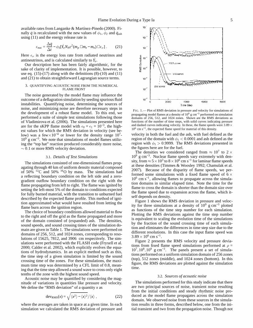
FIG. 1.— Plot of RMS deviation in pressure and velocity for simulations ofpropagating model flames at a density of 109 g cm−3 performed on simulationdomains of 256, 512, and 1024 zones. Shown are the RMS deviations asfunctions of the number of time steps, with solid curves indicating pressureand dashed curves indicating velocity. In these, the flame speeds were 3.89×106 cm s−1, the expected flame speed for material of this density.

velocity in both the fuel and the ash, with fuel defined as theregion of the domain withφ1 < 0.0001 and ash defined as theregion withφ1 > 0.9999. The RMS deviations presented inthe figures here are for the fuel.

The densities we considered ranged from≈ 107 to 2×109 g cm−3. Nuclear flame speeds vary extremely with den-sity, from≈5×103 to 8×106 cm s−1 for laminar flame speedsat these densities (Timmes & Woosley 1992; Chamulak et al.2007). Because of the disparity of flame speeds, we per-formed some simulations with a fixed flame speed of 6×106 cm s−1, allowing flames to propagate across the simula-tion domains in similar elapsed time. Note the time for theflame to cross the domain is shorter than the domain size overthe flame speed due to expansion across the flame, which it-self depends on density.

Figure 1 shows the RMS deviation in pressure and veloc-ity for three simulations at a density of 109 g cm−3 plottedas functions of the time step number for each simulation.Plotting the RMS deviations against the time step numberis equivalent to scaling the evolution time of the simulationsby the fraction of the sound crossing time of each simula-tion and eliminates the differences in time step size due to thedifferent resolutions. In this case the input flame speed was3.89×106 cm s−1.

Figure 2 presents the RMS velocity and pressure devia-tions from fixed flame speed simulations performed atρ =107,108,109 g cm−3. The panels present a set of simula-tions performed on a uniform simulation domain of 256 zones(top), 512 zones (middle), and 1024 zones (bottom). In thisfigure, the RMS deviations are plotted against the simulationtime.

3.2. Sources of acoustic noise

The simulations performed for this study indicate that thereare two principal sources of noise, transient noise resultingfrom the initial conditions and steady rhythmic noise pro-duced as the model flame propagates across the simulationdomain. We observed noise from these sources in the simula-tion results in three forms, described below, one from the ini-tial transient and two from the propagation noise. Though not

6 Townsley et al.

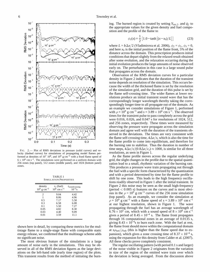
FIG. 2.— Plot of RMS deviations in pressure (solid curves) and ve-locity (dashed curves) for simulations of propagating model flames per-formed at densities of 107 108, and 109 g cm−3 with a fixed flame speed of6× 106 cm s−1. The simulations were performed on a uniform domain with256 zones (top panel), 512 zones (middle panel), and 1024 (bottom panel)zones.

TABLE 1SIMULATION PROPERTIES

density cs (fuel) tsoundcrossing109 g cm−3 108 cm s−1 10−3s

2 9.04 4.421 8.06 4.96

0.5 7.17 5.580.3 6.58 6.080.1 5.50 7.270.05 4.82 8.300.03 4.40 9.090.01 3.59 11.1

shown here in detail, by comparing these metrics for the mul-tistage flame to a single-stage flame with comparable staticenergy release, we confirmed that the multistage scheme addsno significant noise.

The most obvious feature of the simulations is a largeamount of noise early in the simulations. This may be ob-served in all of the RMS deviation figures as the large devi-ations on the left-hand side (early time region) of the plots.This transient results from the method of initiating the burn-

ing. The burned region is created by settingYion, f , andqf tothe appropriate values for the given density and fuel compo-sition and the profile of the flame to

φ1(x) =12

[

1.0− tanh[

(x− x0)/L]]

(23)

whereL = b∆x/2 (Vladimirova et al. 2006),φ2 = φ1, φ3 = 0,and herex0 is the initial position of the flame front, 5% of thedistance across the domain. This prescription produces initialconditions that depart slightly from the relaxed result obtainedafter some evolution, and the relaxation occurring during theinitial evolution produces the large amounts of noise observedearly on. The perturbation in this case is a large sound pulsethat propagates across the domain.

Observation of the RMS deviation curves for a particulardensity in Figure 2 indicates that the duration of the transientnoise depends on resolution of the simulation. This occurs be-cause the width of the thickened flame is set by the resolutionof the simulation grid, and the duration of this pulse is set bythe flame self-crossing time. The wider flames at lower res-olutions produce an initial transient sound wave that has thecorrespondingly longer wavelength thereby taking the corre-spondingly longer time to all propagate out of the domain. Asan example we consider simulations of Figure 1, performedwith ρ = 109 g cm−3 ands= 3.89×106 cm s−1. The observedtimes for the transient pulse to pass completely across the gridwere 0.016, 0.026, and 0.047 s for resolutions of 1024, 512,and 256 zones, respectively. These times were measured byobserving the pressure wave propagate across the simulationdomain and agree well with the duration of the transients ob-served in the deviations. The times are very consistent withthe flame self-crossing time, 4∆x/s, which is also the time forthe flame profile to come into equilibrium, and therefore forthe burning rate to stabilize. Thus the duration in number oftime steps, 4∆x/s/(0.8∆x/cs) ≈ 1000, is similar for all threeresolutions, as seen in Figure 1.

As the flame profile moves across the regular underlyinggrid, the slight changes in the profile due to the spatial quanti-zation lead to a small, rhythmic variation of the burning rate.This produces a pressure wave train propagating out throughthe fuel with a specific form characterized by the quantizationand with a period determined by time for the flame profile toshift by one zone. This leads to the high frequency oscilla-tions readily observed in Figure 1 after the initial transient. InFigure 2 this noise may be seen as the small high-frequency(period< 0.005 s) features on the curves and is most obvi-ous in theρ = 109 g cm−3 curves of the 256 zone simulation(top panel). As an example, we consider the simulation atρ = 109 g cm−3 with a flame speed ofs = 3.89× 106 cm s−1

at our highest resolution, shown in Figure 1. The wavepropagating through the fuel has an average wavelength of6.76×105 cm, which with a sound speed of 8×108 cm s−1

gives a period of 8.45× 10−4 s. The flame front propagatesthrough 16 computational zones in an average of 0.0135 s,giving 8.43×10−4s to burn each zone. With the fuel at rest,the flame front should move within the computational domainat sρfuel/ρash (this is higher than the flame speed due to ex-pansion), which gives a zone crossing time of 8.37×10−4 s,using the expansion for this density from Calder et al. (2007).All these checks prove completely consistent.

The regular oscillating pattern (with period 0.1 s and larger)of the noise visible in Figure 2 originates from the variationin size of the region of the emitted wave train over whichthe deviation is being averaged. From the discussion above

Flame Evolution During a Type Ia 7

this wave train has a wavelength given by equating the soundcrossing time of the disturbance with the time for the flameto cross a single zone,λ/cs = ∆x/vf . Since the sound fieldis otherwise essentially flat, averaging over an integer numberof these wavelengths will give about the same result. Thuswe expect a regular pattern in the noise measured at a perioddetermined by the time for the averaging interval to shrink byone wavelength. The interval is shrinking at the same speedthat the flame is moving across the computational domain,given above, and dividing the wavelength of the emitted trainby this gives a period ofP = λ/vf = cs∆x/(sρfuel/ρash)2. Thisrelation reproduces the linear dependence on resolution seenin the results, and shows that the dependence on density entersthrough both the sound speed and the expansion factor. Wehave confirmed that this relation reproduces the periods in thefigures, e.g.P = 0.24 s fors= 6×106 cm s−1, ρ = 109 g cm−3

and our coarsest resolution. This result represents two bumpsin the noise figures because we are taking the RMS deviation,losing the sign.

Finally, we note that as the flames approached the edge ofthe simulation domain and most of the fuel on the domainhad burned, the magnitude of both the high frequency oscil-lations and the regular pattern in the deviation increased (asmay be observed on the right hand side of the curves, espe-cially at the lowest density, 107 g cm−3). This increase occursbecause what little fuel remains samples the region very nearthe flame, which is expected to have the most noise.

4. THE PROGRESSION OF A FLAME FROM SINGLE-POINTINITIATION

It is useful to describe with some detail the progress ofevents involved in the GCD mechanism, and how our sim-ulation setup captures these events. In the centuries beforethe Ia event, when the WD has accreted enough matter to ig-nite carbon burning in the center, there is an expanding con-vective carbon-burning core (see e.g. Woosley et al. 2004).This state is already a runaway, because the temperature atthe center will continue to monotonically rise. Ignition oc-curs during this convective phase when the local heating timeτheat≃ cPT/ǫnuc, wherecP is the specific heat at constant pres-sure andǫnuc is the nuclear energy deposition rate, becomesshorter than the eddy turnover timeτedd ≃ 10-100 seconds.At this point the burning runs awaylocally, the12C and16Ofuel converts entirely to Fe-peak elements and a flamelet isborn.

While the rate of formation of ignition points is unclear,it is believed that ignition of local flamelets in the core ofthe WD is a fairly stochastic process (Woosley et al. 2004;Wunsch & Woosley 2004). For this study we will work underthe hypothesis that the ignition conditions are rare at the timethe ignition occurs. This means that the ignition grows froma small (. 1 km) region somewhere in the first temperaturescale height (∼ 400 km) near the center of the star, and thesecond ignition is long enough after this (& 1 sec) to be unim-portant (see Woosley et al. 2004 for a discussion of how thesescales arise.) This picture is representative of the ignition con-ditions found by Höflich & Stein (2002) in their study of thepre-runaway phase, but is somewhat in contrast to the conclu-sions of some of the above work (e.g. Woosley et al. 2004),and is essentially the opposite hypothesis to that taken byRöpke et al. (2006a). Single-point ignition is plausible withinthe current uncertainties and is quite useful for our purposehere of understanding the dynamics of a flame bubble andcharacterizing our numerical methods.

4.1. General Simulation Setup

In order to simplify our study of single-bubble dynamics webegin our simulation with no velocity field in the stellar core.This is, in fact, a poor approximation to reality because thetypical outer scale velocity in the convective core is expectedto be∼ 100 km s−1 (Kuhlen et al. 2006), which is compara-ble to the laminar flame propagation speed in this part of thestar (Timmes & Woosley 1992; Chamulak et al. 2007). Thismeans that the strongest initial source of perturbations ontheflame surface, and therefore seeds of the later R-T modes, islikely to be the turbulence in the convective core flow field.The convection field is, however, not strong enough to de-stroy the flamelet once it is born. We feel neglection of thethe convective flow field in this initial study justifiable fortworeasons. First, we would like to understand the dynamics ofthe bubbles and flame surface near the core first without theadditional complication of the turbulent flow. Second, it willbe challenging to interpret the effects that a turbulent field intwo dimensions subject to the imposed axisymmetry mightproduce. Any off-axis feature acts effectively as a ring, anef-fect that causes enough difficulty even with static initial con-ditions. Also Livne et al. (2005) find that the general outcomeof off-center ignitions is not strongly effected by the presenceof a convection field.

We perform two-dimensional axisymmetric simulationswith the FLASH adaptive-mesh hydrodynamics code(Fryxell et al. 2000; Calder et al. 2002). We begin oursimulations with at 1.38M⊙ WD with a uniform compositionof equal parts by mass of12C and16O. This model has acentral density of 2.2× 109 g cm−3, a uniform temperatureof 4× 107 K, and a radius of approximately 2,000 km. Aspherical region on the symmetry axis is converted to burnedmaterial with φ1 given by eq. (23) withx = |~r −~roff | andx0 = rbub, φ2 = φ1, andφ3 = 0, where~roff is the location of thecenter of the ignition point. The density is chosen to maintainpressure equilibrium with the surrounding material. Thus theradius of the flame bubble,rbub, is the approximate locationof the φ1 = 0.5 isosurface, and all simulations in this paperbegin with a spherical bubble of radius 16 km. This is thesmallest bubble that is reasonably well resolved (havingφ1very close to 1 at the center) at 4 km resolution, that usedin the parameter study presented in section 5. The basicparameters and some results are listed in Table 2, and will bediscussed below.

Our adaptive mesh refinement has been chosen to capturethe relevant physical features of the burning and flow at rea-sonable computational expense. We choose to refine on strongdensity gradients everywhere, and strong velocity gradients inthe burned material. At the beginning of the simulation all ofthe star is resolved to 16 km resolution regardless of the max-imum allowed resolution for reasons of hydrostatic stability(Plewa 2007). In regions withρ < 5× 105 g cm−3 refine-ment is not requested, which includes all of the region out-side the star. Regions where the flame is actively propagating(0.1 < φ < 0.9, and non-trivial flame speed) are required tobe fully refined in order to properly propagate the flame front.In the interest of limiting computational expense, the refine-ment is limited to a finest resolution of 32 km outside a radiusof 2500 km, which is above the the surface of the star in allcases treated here. This constraint will be relaxed in futurework, but the bulk kinetic motion of the surface flow is notexpected to be affected by this choice.

8 Townsley et al.

0 100 200 300 400 500radius (km)

1

10

100λ c (

km)

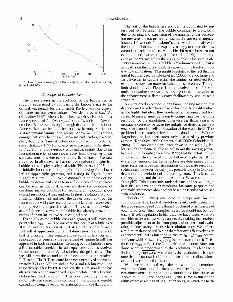
FIG. 3.— Critical wavelength for flame surface perturbationsλc = 6πs2/Agin the initial WD.

4.2. Stages of Flamelet Evolution

The major stages in the evolution of the bubble can beroughly understood by comparing the bubble’s size to thecritical wavelength for the unstable Rayleigh-Taylor growthof flame surface perturbations. We defineλc ≡ 6πs2/Ag(Khokhlov 1995), whereg is the local gravity,s is the laminarflame speed, andA = (ρfuel − ρash)/(ρfuel + ρash) is the Atwoodnumber. Belowλc, s is high enough that perturbations in theflame surface can be “polished out” by burning, so that thesurface remains laminar and simple. Aboveλc, R-T is strongenough that perturbations will grow instead, leading to a com-plex, disordered flame structure down to a scale of orderλc.(See Khokhlov 1995 for an extensive discussion.) As shownin Figure 3,λc drops quickly with radius, mainly due to theincreasing gravity as one moves away from the center of thestar, and after this due to the falling flame speed. We takerbub < λc in all cases, so that our assumption of a sphericalbubble at rest is physically justifiable (Fisher et al. 2007).

Initially bubbles can be thought of as moving from lowerleft to upper right (growing and rising) in Figure 3 (seeZingale & Dursi 2007). We distinguish three phases of thebubble evolution and rise in terms ofλc. Each of these phasescan be seen in Figure 4, where we show the evolution ofthe flame surface with time for two different resolutions: ourtypical resolution, 4 km, and our highest resolution, 0.5 km.Initially, while small and near the center withrbub < λc, theflame bubble will grow according to the laminar flame speed,roughly keeping a spherical shape. This structure is evidentat t = 0.2 seconds, where the bubble has already grown to aradius of about 30 km, twice its original size.

Eventually as the bubble rises and grows, it will reach thepoint whenrbub∼ λc. For our case this occurs at a little over100 km radius. As seen att = 0.4 sec, the bubble forms aR-T roll at approximately its full dimensions, the first scalethat is unstable. This feature shows some differences withresolution, but generally the same kind of feature (a roll) hasappeared in both simulations. Crossingλc, the bubble is nowa R-T unstable flamelet. The subsequent evolution is resolvedin our simulation untilλc falls below the grid scale. Thuswe will term the second stage of evolution as the resolvedR-T stage. The R-T structure becomes unresolved at approx-imately 350 and 500 km radius for 4 and 0.5 km resolutionrespectively. Thus by t=0.6 seconds, the 4 km simulation hasalready entered the unresolved regime, while the 0.5 km sim-ulation has nearly entered it. This is evidenced by the sepa-ration between consecutive contours in the progress variablecaused by strong advection of material within the flame front.

The rest of the bubble rise and burn is dominated by un-resolved R-T burning. The bubble continues to grow, bothdue to burning and expansion of the material under decreas-ing pressure. Its top generally reaches the surface at approx-imately 1.0 seconds (“breakout”), after which it mostly exitsthe interior of the star and expands strongly to create the flowaround the stellar surface. A notable difference between ourevolution and that seen by (Röpke et al. 2006b) is the pres-ence of the “stem” below the rising bubble. This stem is ab-sent in non-reactive rising bubbles (Vladimirova 2007), but itis mysterious that it is completely absent in the level-set reac-tive flow simulations. This might be related to the fact that theinitial bubbles used by Röpke et al. (2006b) are too large andfar off-center to capture either the laminar or resolved R-Tevolution stages, but more investigation is necessary. Thoughboth simulations in Figure 4 are unresolved att = 0.8 sec-onds, comparing the two provides a good demonstration ofthe enhancement in flame surface facilitated by smaller scalestructure.

As mentioned in section 2, any flame tracking method thatdepends on the advection of a scalar field faces difficultiesin the highly turbulent flow produced in the unresolved R-Tstage. Measures must be taken to compensate for the finiteresolution of the simulation, otherwise the flame ceases topropagate correctly because the turbulence destroys the nec-essary structure for self-propagation of the scalar field. Thisproblem is particularly relevant to the simulation of WD de-flagrations, as has been extensively discussed by previousauthors (Khokhlov 1995; Gamezo et al. 2003; Schmidt et al.2006). R-T can create turbulence down to the scaleλc, be-low which the flame is able to polish out the mixing pertur-bations. It is thought (Khokhlov 1995) that the details of thissmall-scale behavior need not be followed explicitly. If theoverall dynamics of the flame surface are determined by thelarge scale perturbations, simulations of moderate resolution(which may however be only just possible today in 3-d) candetermine the evolution of the burning front. This is calledself-regulation, and the open question is: What resolutionis“enough”? This is currently under debate, and we will arguehere that we have enough resolution for some purposes andcan make statements about others based on trends that we seewith resolution.

Schmidt et al. (2006) attempted to compensate for theshortcoming of the limited resolution by artificially enhancingthe propagation speed of the flame front based on a measure oflocal turbulence. Such complex measures should not be nec-essary if self-regulation holds, thus we have taken what weconsider to be a conservative approach, making the smallestpossible adjustment to the front propagation speed and evalu-ating the inaccuracy directly via resolution study. We enforcea minimum flame speed (which therefore acts effectively as anenhancement) that is intended to ensureτR−T & τflame where,for flame widthδ, τR−T ≈

√

δ/Ag is the characteristic R-T risetime andτflame≈ δ/s is the flame self-crossing time. Since ourflame width is proportional to the resolution, this leads to alimit s≥ α

√

Agmf ∆x, where∆x is the resolution,α is a ge-ometrical factor that is different in two and three dimensions,andmf is a calibrated constant.

We have determinedmf , the constant that determineswhen the flame model “breaks”, empirically by runningtwo-dimensional flame-in-a-box simulations like those ofKhokhlov (1995) and Zhang et al. (2007). We evaluated therange ofsover which self-regulation holds, in which the burn-

Flame Evolution During a Type Ia 9

FIG. 4.— Stages of bubble growth at different resolutions. The initial radius of the bubble was 16 km centered at 40 km from thecenter of the star, contoursare shown for the progress variableφ = 0.1 (green), 0.5 (red), and 0.9 (blue).

ing rate,mburned= ρL(d−1)seff is determined by the box size,L, such thatseff = α

√AgL, independent ofs. In two dimen-

sionsα = 0.28 and in three dimensions, as found by previ-ous authors,α = 0.5. We found that the self-regulated regimeis bounded above bys ≃ √

AgL, corresponding to the re-quirementλc . L, and below bys≃ α

√Ag0.04∆x. In our

WD simulations we have used the value forα from three-dimensional simulations, although we are working in two-dimensional cylindrical geometry, andmf = 0.04. These val-ues have been confirmed by preliminary three-dimensionalflame-in-a-box calculations, which will be discussed in a sep-arate work. Using this type of floor ons requires that weexplicitly turn off the flame at low density. This is donesmoothly betweenρ = 107 g cm−3 and 5×106 g cm−3, so thats= 0 for densities below this.

4.3. Resolution Study

Some properties of the off-center deflagration model thatwe are trying to deduce from our simulations show depen-dence on the simulation resolution, while others do not. Wewould like to make statements as much as possible based onfeatures that are not influenced by resolution, and where wecannot avoid it, account for the dependence in other conclu-sions that we draw. Problems with resolution-dependence isnot entirely unexpected, since, as just discussed, a significantamount of our simulation isa priori known to be unresolved.In summary, we find that the conditions at the possible deto-nation point are fairly insensitive to resolution, for the reso-lutions considered, but that the state of the interior of thestarat a given time during the runaway may only be calculatedby higher resolution simulations than the 4 km at which ourparameter study was performed.

Of foremost interest is the robustness of the gravitationallyconfined detonation (GCD) mechanism, particularly the prop-erties in the collision and compression regions opposite the

10 Townsley et al.

0

1

2

3

4

5

6

Tm

ax u

nbur

ned

(109 K

)

8 km4 km2 km1 km

1 1.5 2 2.5time (s)

105

106

107

Den

sity

at T

max

(g

cm-3

)

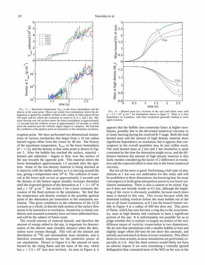
FIG. 5.— Maximum temperatureTmax in the lower hemisphere and thedensity at the same point. Shown are results from simulations where the de-flagration is ignited by a bubble of flame with a radius of 16km placed 40 kmoff-center and for which the resolution is varied to 8, 4, 2, and 1 km. Ma-terial flowing over the surface enters the lower hemisphere at approximately1.5 seconds and the collision occurs at approximately 2.0 seconds, at whichpoint the material near the collision region begins to compress. We find thatthe conditions at the ignition point are insensitive to the simulation resolution.

eruption point. We have performed two-dimensional simula-tions of various resolutions that begin from a 16 km radiusburned region offset from the center by 40 km. The historyof the maximum temperature,Tmax, in the lower hemisphere(θ > π/2), and the density at that same point is shown in Fig-ure 5. After the bubble has reached the surface, material –burned and unburned – begins to flow over the surface ofthe star towards the opposite pole. This material enters thelower hemisphere approximately 1.5 seconds after the igni-tion. Some of the low-density material is being shocked asit interacts with the stellar surface as it is moving around thestar, giving a temperature near 109 K. The collision of mate-rial at the lower pole occurs at approximately 2 seconds andthe density of the hottest region steadily increases thereafteruntil the expected ignition of the detonation atT > 3×109 Kandρ > 107 g cm−3. See section 5 for a more extensive dis-cussion of the fluid motions in the simulation. We find thatthe temperature and density reached at the possible ignitionpoint of the detonation are insensitive to the simulation res-olution. This gives confidence in the robustness of the GCDscenario as a whole, in that the bulk motion of the surface flowseems to be insensitive to resolution. Sensitivity to initial con-ditions and assumed symmetry have not been addressed here,and will be the subject of future work.

The overall amount of material burned, and therefore theamount of energy added to the star, is important for determi-nation of the interior state (notably density) when the deto-nation wave sweeps through. This will set the amount anddistribution of 56Ni and intermediate mass elements, and istherefore extremely important for the predictive power ofour simulations. Shown in Figure 6 is the amount of massburned by the rising flame and the mass of the star, whichhasρ > 5.5×107 (see next section). As seen in Figure 4, it

0

0.5

1

1.5

2

2.5

3

Mas

s bu

rned

(%

of s

tar)

0 0.5 1 1.5 2 2.5time (s)

0.8

0.9

1

1.1

1.2

Mas

s at

hig

h de

nsity

(M O·)

8 km

42

1

8 km

4

2

1

FIG. 6.— Burned mass (as a fraction of the star) and stellar mass withρ > 5.5× 107 g cm−3 for simulations shown in figure 5. There is a cleardependence on resolution, with finer resolutions generallyleading to morerapid evolution.

appears that the bubble rises somewhat faster at higher reso-lutions, possibly due to the decreased numerical viscosityorto faster burning during the resolved R-T stage. Both the totalburned mass and the amount of high density material showsignificant dependence on resolution, but it appears that con-vergence in the overall quantities may be just within reach.The total burned mass at 2 km and 1 km resolution is quiteconsistent by the time the detonation might occur, and the dif-ference between the amount of high density material is alsofairly modest considering the factor of 2 difference in resolu-tion and the expected offset in time due to the lower numericalviscosity.

But not all the news is good. Performing a full suite of sim-ulations at 1 km was not undertaken for this study and willbe prohibitive in three dimensions, but knowing how far awayconvergence is lends great interpretive power to our lower res-olution simulations. There is also a caution to be raised. Fig-ure 6 does not include results at 0.5 km, although the begin-ning of the curve is obviously available, because much moremass is burned in this case. This occurs because while thedominant trailing vortices follow the main bubble out of thestar at all lower resolutions, at 0.5 km the branch feature vis-ible in Figure 4 at a radius of 600 km does not. This pieceof flame, which has now become a ring due to the axisymme-try, stays at high density and continues to burn a significantportion of the star. It is unfortunately not possible for us tojudge whether this is realistic or largely an artifact of theverydifferent nature of vorticity conservation in two dimensions.We do note that simulations with a smaller bubble (2 km) andslightly larger offset (60 km) do not show this anomaly, andinitially proceed much as those at lower resolution. This effectdeserves close scrutiny as more simulations are performed,es-pecially in 3-d. Also the shed vortices would likely not havean adverse impact if we were simulating a centrally igniteddeflagration that consumed most of the WD on the way to the

Flame Evolution During a Type Ia 11

0

1

2

3

4

5

6

Tm

ax u

nbur

ned

(109 K

)

1 1.5 2 2.5 3time (s)

105

106

107

Den

sity

at T

max

(g

cm-3

)

20 km

4050

80

100

20 km

4050

80

100

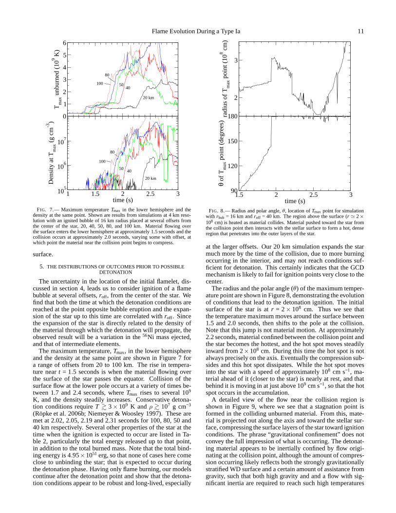
FIG. 7.— Maximum temperatureTmax in the lower hemisphere and thedensity at the same point. Shown are results from simulations at 4 km reso-lution with an ignited bubble of 16 km radius placed at several offsets fromthe center of the star, 20, 40, 50, 80, and 100 km. Material flowing overthe surface enters the lower hemisphere at approximately 1.5 seconds and thecollision occurs at approximately 2.0 seconds, varying some with offset, atwhich point the material near the collision point begins to compress.

surface.

5. THE DISTRIBUTIONS OF OUTCOMES PRIOR TO POSSIBLEDETONATION

The uncertainty in the location of the initial flamelet, dis-cussed in section 4, leads us to consider ignition of a flamebubble at several offsets,roff , from the center of the star. Wefind that both the time at which the detonation conditions arereached at the point opposite bubble eruption and the expan-sion of the star up to this time are correlated withroff . Sincethe expansion of the star is directly related to the density ofthe material through which the detonation will propagate, theobserved result will be a variation in the56Ni mass ejected,and that of intermediate elements.

The maximum temperature,Tmax, in the lower hemisphereand the density at the same point are shown in Figure 7 fora range of offsets from 20 to 100 km. The rise in tempera-ture neart = 1.5 seconds is when the material flowing overthe surface of the star passes the equator. Collision of thesurface flow at the lower pole occurs at a variety of times be-tween 1.7 and 2.4 seconds, whereTmax rises to several 109

K, and the density steadily increases. Conservative detona-tion conditions requireT & 3× 109 K and ρ & 107 g cm−3

(Röpke et al. 2006b; Niemeyer & Woosley 1997). These aremet at 2.02, 2.05, 2.19 and 2.31 seconds for 100, 80, 50 and40 km respectively. Several other properties of the star at thetime when the ignition is expected to occur are listed in Ta-ble 2, particularly the total energy released up to that point,in addition to the total burned mass. Note that the total bind-ing energy is 4.95×1051 erg, so that none of cases here comeclose to unbinding the star; that is expected to occur duringthe detonation phase. Having only flame burning, our modelscontinue after the detonation point and show that the detona-tion conditions appear to be robust and long-lived, especially

2

3

radi

us o

f Tm

ax p

oint

(10

8 cm

)

1.5 2 2.5 3time (s)

90

120

150

180

θ of

Tm

ax p

oint

(de

gree

s)

FIG. 8.— Radius and polar angle,θ, location ofTmax point for simulationwith rbub = 16 km androff = 40 km. The region above the surface (r ≃ 2×108 cm) is heated as material collides. Material pushed toward the star fromthe collision point then interacts with the stellar surfaceto form a hot, denseregion that penetrates into the outer layers of the star.

at the larger offsets. Our 20 km simulation expands the starmuch more by the time of the collision, due to more burningoccurring in the interior, and may not reach conditions suf-ficient for detonation. This certainly indicates that the GCDmechanism is likely to fail for ignition points very close tothecenter.

The radius and the polar angle (θ) of the maximum temper-ature point are shown in Figure 8, demonstrating the evolutionof conditions that lead to the detonation ignition. The initialsurface of the star is atr = 2× 108 cm. Thus we see thatthe temperature maximum moves around the surface between1.5 and 2.0 seconds, then shifts to the pole at the collision.Note that this jump is not material motion. At approximately2.2 seconds, material confined between the collision point andthe star becomes the hottest, and the hot spot moves steadilyinward from 2×108 cm. During this time the hot spot is notalways precisely on the axis. Eventually the compression sub-sides and this hot spot dissipates. While the hot spot movesinto the star with a speed of approximately 108 cm s−1, ma-terial ahead of it (closer to the star) is nearly at rest, and thatbehind it is moving in at just above 109 cm s−1, so that the hotspot occurs in the accumulation.

A detailed view of the flow near the collision region isshown in Figure 9, where we see that a stagnation point isformed in the colliding unburned material. From this, mate-rial is projected out along the axis and toward the stellar sur-face, compressing the surface layers of the star toward ignitionconditions. The phrase “gravitational confinement” does notconvey the full impression of what is occurring. The detonat-ing material appears to be inertially confined by flow origi-nating at the collision point, although the amount of compres-sion occurring likely reflects both the strongly gravitationallystratified WD surface and a certain amount of assistance fromgravity, such that both high gravity and and a flow with sig-nificant inertia are required to reach such high temperatures

12 Townsley et al.

TABLE 2PROPERTIES ATDETONATION IGNITION

rbub roff resolution tdeta Mburn mass at high density max density energy release

(km) (km) (km) (s) (% of star) (M⊙) (108 g cm−3) (1050 erg)

Resolution Study

16 40 8 2.35 1.97 1.04 7.6 0.32916 40 4 2.31 2.33 1.01 6.6 0.38816 40 2 2.37 2.90 0.926 5.0 0.47816 40 1 2.35b 2.88 0.892 4.5 0.517

Offset Study

16 100 4 2.02 1.13 1.13 12 0.19316 80 4 2.05 1.36 1.12 11 0.22616 50 4 2.19 2.07 1.05 8.0 0.34716 40 4 2.31 2.33 1.01 6.6 0.38816 20 4 2.70c 6.57 0.473 1.6 1.15

NOTE. — All values are evaluated at the time indicated,tdet.a tdet is defined as the first time at whichρ > 107 g cm−3 at the point ofTmax > 3× 109 K.b In this case wehave neglected the early, short-lived, fluctuation att ≃ 2.15 sc Our conservative detonation criteria are notreached, listed are values for the peak density of theTmax point.

and densities. The collision itself arises because the mate-rial is gravitationally bound, however, it is the kinetic motionimparted to the material by the expanded bubble at the break-out point that eventually leads to the (gravitationally assisted)confinement.

In the GCD scenario, because so little material is burnedduring the deflagration phase, the amount of56Ni produced inthe supernova is determined by the density distribution duringthe detonation phase. In lieu of simulating the propagationofthe detonation, which will be performed in future work, wehave measured the mass of material above 5.5×107 g cm−3.This limit is obtained from the density at which material inthe W7 model (Nomoto et al. 1984) burned to only 50%56Ni.This is obviously only a rough estimate, but is good enoughfor measuring the trend with offset distance that we are in-terested in here. The bottom panel of Figure 10 shows howthis possible56Ni mass decreases as the star expands duringthe deflagration phase. The curves are marked at the expectedlaunch time of the detonation, where the temperature and den-sity first exceed 3×109 K and 107 g cm−3 together.

We find that the amount of56Ni expected in the ejecta iscorrelated with the offset of the initial (small) ignition region.Larger offsets can produce more56Ni for two reasons: (1) lessenergy is released in the deflagration phase, and therefore thestar has expanded less when the detonation occurs, and (2) thedetonation conditions happen sooner so that the star has hadless time to expand. It does appear that the first of these is thedominant effect. The top panel of Figure 10 shows the massburned as a fraction of the star with time. Larger offsets burnless of the star during the bubble rise and breakout, leadingtoless expansion of the star.

The56Ni mass estimates we have found here are fairly high,but as seen in section 4.3 this resolution (4 km) appears tosomewhat underestimate the burned mass and overestimatethe possible56Ni at the detonation time. We are not claimingto have performed an absolute calculation of the56Ni mass fora given ignition point offset; we have instead demonstrateda trend that appears to be robust with respect to the physi-cal processes that are occurring. We hope that in the future,with higher resolution such that self-regulation of the burningis strong enough that we can constrain the R-T phase better,we may be able to construct a fully predictive model. There

are, however several steps that should be taken in the meantime, including three-dimensional studies that are underway(Jordan et al. 2007), and studies of flame bubble response tothe strong convection expected to be present in the WD corewhen the ignition occurs. The current level of calculation is,however sufficient for measuring trends such as how thingsmight change with the relative C/O fraction in the interior ofthe WD.

6. CONCLUSIONS

We have shown that in the GCD picture of a delayed deto-nation of a WD near the Chandrasekhar mass, the propertiesof the WD at detonation, notable the density distribution, aresystematically correlated with the offset of the ignition pointof the deflagration. Assuming that the detonation phase pro-ceeds as in previous simulations, this will cause a variation inthe 56Ni mass ejected in the supernova. The position of theignition point within the inner few 100 km of the WD is ex-pected to be stochastically determined by the turbulent flowin this region. GCD thus provides a possible explanation forthe variety of56Ni masses seen in Type Ia Supernovae.

We find that the conditions (temperature and densityreached) at the candidate launch point of the detonation areinsensitive to the resolution of the simulation for resolutionsstudied here (≤ 8 km). This is a good mark for the robustnessof the GCD mechanism, but more work is needed, especiallyrelated to the possibility of vortex shedding early in the bub-ble rise and the strong convection that should be present in thecore at the time of ignition. We have indications of numeri-cal convergence in both the total burned mass and the massof dense material, and therefore the predicted56Ni mass pro-duced by a given ignition offset. But caution is advisable: themass burned during the highly Rayleigh-Taylor (buoyancy-driven) unstable rise of the burned region through the star isseen to vary with resolution, generally progressing fasterwithhigher resolution, even though convergence in the final valueappears to have been reached. Also, converged results (in theextremely limited sense indicated here) appear to require 2km or possibly 1 km resolution, which is prohibitive in threedimensions. Even here, our parameter study has been per-formed at 4 km resolution for efficiency. Thus we are able topredict trends in the56Ni mass, but not the actual value ejectedfor a given offset.

Flame Evolution During a Type Ia 13

FIG. 9.— Detail of flow near the collision and detonation region for theroff = 40 km case, from top to bottom att = 2.07, 2.19, and 2.32 seconds.Temperature is shown in color and contours are shown atρ = 107 g cm−3

(blue) and at the edge of the burned material (φ = 0.1, red). Velocity vectorssmaller that 108 cm s−1 are not shown. A stagnation point is formed abovethe surface of the star from which material is projected out along the axis andcompressed against the surface of the star, where the detonation is expectedto occur.

0

0.5

1

1.5

2

2.5

3

Mas

s bu

rned

(%

of s

tar)

0 0.5 1 1.5 2 2.5time (s)

0.95

1

1.05

1.1

1.15

1.2

Mas

s at

hig

h de

nsity

(M O·)

20 km 40

50

80

100

50

40

20 km

80

100

FIG. 10.— Burned mass (as a fraction of the star) and stellar masswithρ > 5.5×107 g cm−3 for same simulations as in Figure 7. The time at whicha detonation is expected to be launched is marked with a× for each case.Larger offsets are expected to produce more56Ni in the ejected material.

Our method for following the nuclear energy release, in-cluding neutronization, with an ADR flame model was de-scribed in detail. This method reproduces the energy releaseand hydrodynamic characteristics of the nuclear burning byfollowing a limited number of parameters coupled to an arti-ficially thickened flame front. We have demonstrated that theenergy release adds a minimal amount of unwanted acousticnoise (RMS velocity< few×10−4) to the simulation, largelyremoving this source of unrealistic seeds for the instabilitiesin the rising flame surface.

The authors thank Alexei Khokhlov for encouragementand insight during development of the flame model, RobertFisher for enlightening discussions during the later stages ofthis work, George Jordan for preliminary work implement-ing an electron-ion formalism in Flash, the code group at theASC/Flash center, especially Anshu Dubey and Dan Sheeler,for support in code development, and Ed Brown for commentson the manuscript. This work is supported at the Universityof Chicago in part by the National Science Foundation un-der Grant PHY 02-16783 for the Frontier Center “Joint In-stitute for Nuclear Astrophysics” (JINA), and in part by theU.S. Department of Energy under Contract B523820 to theASC Alliances Center for Astrophysical Flashes. ACC ac-knowledges support from the NSF grant AST-0507456. JWTacknowledges support from Argonne National Laboratory,which is operated under contract No. W-31-109-ENG-38 withthe DOE.

14 Townsley et al.

REFERENCES

Asida, S., Townsley, D. M., Calder, A. C., Zhiglo, A., Jena, T., Khokhlov, A.,& Lamb, D. Q. 2007, ApJ, in preparation

Calder, A. C., Fryxell, B., Plewa, T., Rosner, R., Dursi, L. J., Weirs, V. G.,Dupont, T., Robey, H. F., Kane, J. O., Remington, B. A., Drake, R. P.,Dimonte, G., Zingale, M., Timmes, F. X., Olson, K., Ricker, P., MacNeice,P., & Tufo, H. M. 2002, ApJS, 143, 201

Calder, A. C., Plewa, T., Vladimirova, N., Lamb, D. Q., & Truran, J. W. 2004,ArXiv Astrophysics e-prints, astro-ph/0405162

Calder, A. C., Townsley, D. M., Seitenzahl, I. R., Peng, F., Messer, O. E. B.,Vladimirova, N., Brown, E. F., Truran, J. W., & Lamb, D. Q. 2007, ApJ,656, 313

Chamulak, D. A., Brown, E. F., & Timmes, F. X. 2007, ApJ, 655, L93Fisher, R. T., Vladimirova, N., Jordan, G. C., & Lamb, D. Q. 2007, ApJ, in

preparationFryxell, B., Olson, K., Ricker, P., Timmes, F. X., Zingale, M., Lamb, D. Q.,

MacNeice, P., Rosner, R., Truran, J. W., & Tufo, H. 2000, ApJS, 131, 273Gamezo, V. N., Khokhlov, A. M., & Oran, E. S. 2004, Physical Review

Letters, 92, 211102—. 2005, ApJ, 623, 337Gamezo, V. N., Khokhlov, A. M., Oran, E. S., Chtchelkanova, A. Y., &

Rosenberg, R. O. 2003, Science, 299, 77Höflich, P. & Stein, J. 2002, ApJ, 568, 779Hillebrandt, W. & Niemeyer, J. C. 2000, ARA&A, 38, 191Jordan, G. C., Fisher, R., Townsley, D. M., Calder, A. C., Asida, S., Graziani,

C., Lamb, D. Q., & Truran, J. W. 2007, ApJ, submittedKhokhlov, A. M. 1983, Soviet Astronomy Letters, 9, 160—. 1991, A&A, 245, 114—. 1995, ApJ, 449, 695—. 2000, ArXiv Astrophysics e-prints, astro-ph/0008463Kuhlen, M., Woosley, S. E., & Glatzmaier, G. A. 2006, ApJ, 640, 407

Langanke, K. & Martínez-Pinedo, G. 2000, Nuclear Physics A,673, 481Livne, E., Asida, S. M., & Höflich, P. 2005, ApJ, 632, 443Niemeyer, J. C. & Woosley, S. E. 1997, ApJ, 475, 740Nomoto, K., Thielemann, F.-K., & Yokoi, K. 1984, ApJ, 286, 644Plewa, T. 2007, ApJ, in press. (astro-ph/0611776)Plewa, T., Calder, A. C., & Lamb, D. Q. 2004, ApJ, 612, L37Reinecke, M., Hillebrandt, W., Niemeyer, J. C., Klein, R., &Gröbl, A. 1999,

A&A, 347, 724Röpke, F. K., Hillebrandt, W., Niemeyer, J. C., & Woosley, S.E. 2006a,

A&A, 448, 1Röpke, F. K., Niemeyer, J. C., & Hillebrandt, W. 2003, ApJ, 588, 952Röpke, F. K., Woosley, S. E., & Hillebrandt, W. 2006b, ApJ, Submitted.

(astro-ph/0609088)Schmidt, W., Niemeyer, J. C., Hillebrandt, W., & Röpke, F. K.2006, A&A,

450, 283Smiljanovski, V., Moser, V., & Klein, R. 1997, Combustion Theory

Modelling, 1, 183Timmes, F. X. & Swesty, F. D. 2000, ApJS, 126, 501Timmes, F. X. & Woosley, S. E. 1992, ApJ, 396, 649Vladimirova, N. 2007, Comb. Theory and modelling, 11, 377Vladimirova, N., Weirs, G., & Ryzhik, L. 2006, Combust. Theory Modelling,

10, 727Woosley, S. E., Wunsch, S., & Kuhlen, M. 2004, ApJ, 607, 921Wunsch, S. & Woosley, S. E. 2004, ApJ, 616, 1102Xin, J. 2000, SIAM Review, 42, 161Zhang, J., Messer, O. E. B., Khokhlov, A. M., & Plewa, T. 2007,ApJ, 656,

347Zingale, M. & Dursi, L. J. 2007, ApJ, 656, 333