Finding All Covers of an Indeterminate String in O(n) Time on Average
280
Proceedings of the Prague Stringology Conference 2009 Edited by Jan Holub and Jan ˇ Zd ’ ´arek Department of Computer Science and Engineering August 2009 Prague Stringology Club http://www.stringology.org/
-
Upload
independent -
Category
Documents
-
view
0 -
download
0
Transcript of Finding All Covers of an Indeterminate String in O(n) Time on Average

Proceedings of the
Prague Stringology Conference 2009
Edited by Jan Holub and Jan Zd’arek
Department of Computer Scienceand Engineering
August 2009
Prague Stringology Clubhttp://www.stringology.org/

Proceedings of the Prague Stringology Conference 2009Edited by Jan Holub and Jan Zd’arekPublished by: Prague Stringology Club
Department of Computer Science and EngineeringFaculty of Electrical EngineeringCzech Technical University in PragueKarlovo namestı 13, Praha 2, 121 35, Czech Republic.
URL: http://www.stringology.org/E-mail: [email protected] Phone: +420-2-2435-7470 Fax: +420-2-2492-3325Printed by Ceska technika–Naklatelstvı CVUT, Thakurova 550/1, Praha 6, 160 41, Czech Republic
c© Czech Technical University in Prague, Czech Republic, 2009
ISBN 978-80-01-04403-2

Conference Organization
Program Committee
Amihood Amir (Bar-Ilan University, Israel)Gabriela Andrejkova (P. J. Safarik University, Slovakia)Maxime Crochemore (Universite de Marne la Vallee, France)Frantisek Franek (McMaster University, Canada)Jan Holub, Co-chair (Czech Technical University in Prague, Czech Republic)Costas S. Iliopoulos (King’s College London, United Kingdom)Shmuel T. Klein (Bar-Ilan University, Israel)Thierry Lecroq (Universite de Rouen, France)Borivoj Melichar, Co-chair (Czech Technical University in Prague, Czech Republic)Yoan J. Pinzon (King’s College London, United Kingdom)Marie-France Sagot (Universite Claude Bernard, Lyon, France)William F. Smyth (McMaster University, Canada)Bruce W. Watson (Technische Universiteit Eindhoven, Netherlands)
Organizing Committee
Miroslav Balık, Co-chairJan Holub, Co-chair
Jan JanousekBorivoj Melichar
Ladislav VagnerJan Zd’arek
External Referees
Saıd AbdeddaımPavlos AntoniouMiroslav BalıkManolis ChristodoulakisLoek CleophasJacqueline DaykinSimone FaroMathieu GiraudSzymon Grabowski
Ondrej GuthJan JanousekDerrick KourieJan LahodaArnaud LefebvreJuan MendivelsoSpiros MichalakopoulosErnest Ketcha NgassamSolon Pissis
Elise PrieurPetr ProchazkaGiuseppina RindoneGerman TischlerWilson SotoTinus StraussMichal Ziv-Ukelson

iv

Preface
The proceedings in your hands contains the papers presented in the Prague Stringol-ogy Conference 2009 (PSC’09) which was held at the Department of Computer Sci-ence and Engineering of the Czech Technical University in Prague, Czech Republic,on August 31–September 2. The conference focused on stringology and related top-ics. Stringology is a discipline concerned with algorithmic processing of strings andsequences.
The papers submitted were reviewed by the program committee and twenty threewere selected for presentation at the conference, based on originality and quality. Thisvolume contains not only these selected papers but also abstract of one invited talkdevoted to the combination of text compression and string matching.
The Prague Stringology Conference has a long tradition. PSC’09 is the fourteenthevent of the Prague Stringology Club. In the years 1996–2000 the Prague Stringol-ogy Club Workshops (PSCW’s) and the Prague Stringology Conferences (PSC’s) in2001–2006, 2008 preceded this conference. The proceedings of these workshops andconferences had been published by the Czech Technical University in Prague andare available on WWW pages of the Prague Stringology Club. Selected contributionswere published in special issues of journals the Kybernetika, the Nordic Journal ofComputing, the Journal of Automata, Languages and Combinatorics, and the In-ternational Journal of Foundations of Computer Science. The series of stringologyconferences was interrupted in 2007 when the members of the Prague StringologyClub were honoured to organize Conference on Implementation and Application ofAutomata 2007 (CIAA 2007).
The Prague Stringology Club was founded in 1996 as a research group at theDepartment of Computer Science and Engineering of the Czech Technical Universityin Prague. The goal of the Prague Stringology Club is to study algorithms on strings,sequences, and trees with emphasis on finite automata theory. The first event orga-nized by the Prague Stringology Club was the workshop PSCW’96 featuring only ahandful of invited talks. However, since PSCW’97 the papers and talks are selectedby a rigorous peer review process. The objective is not only to present new resultsin stringology and related areas, but also to facilitate personal contacts among thepeople working on these problems.
I would like to thank all those who had submitted papers for PSC’09 as well as thereviewers. Special thanks go to all the members of the program committee, withoutwhose efforts it would not have been possible to put together such a stimulating pro-gram of PSC’09. Last, but not least, my thanks go to the members of the organizingcommittee for ensuring such a smooth running of the conference.
In Prague, Czech Republicon August 2009
Jan Holub
v

vi

Table of Contents
Invited Talk
Combining Text Compression and String Matching: The Miracle ofSelf-Indexing by Gonzalo Navarro . . . . . . . . . . . . . . . . . . . . . . . . . . . . . . . . . . . . . . . 1
Contributed Talks
Feature Extraction for Image Pattern Matching with Cellular Automata byLynette van Zijl and Leendert Botha . . . . . . . . . . . . . . . . . . . . . . . . . . . . . . . . . . . . . 3
On-line construction of a small automaton for a finite set of words byMaxime Crochemore and Laura Giambruno . . . . . . . . . . . . . . . . . . . . . . . . . . . . . . . 15
Adapting Boyer-Moore-Like Algorithms for Searching Huffman EncodedTexts by Domenico Cantone, Simone Faro, and Emanuele Giaquinta . . . . . . . . . 29
Finding Characteristic Substrings from Compressed Texts by ShunsukeInenaga and Hideo Bannai . . . . . . . . . . . . . . . . . . . . . . . . . . . . . . . . . . . . . . . . . . . . . 40
Delta Encoding in a Compressed Domain by Shmuel T. Klein and Moti Meir . . 55
On Bijective Variants of the Burrows-Wheeler Transform by Manfred Kufleitner 65
On the Usefulness of Backspace by Shmuel T. Klein and Dana Shapira . . . . . . . 80
An Efficient Algorithm for Approximate Pattern Matching with Swaps byMatteo Campanelli, Domenico Cantone, Simone Faro, and Emanuele Giaquinta 90
Searching for Jumbled Patterns in Strings by Ferdinando Cicalese, GabrieleFici, and Zsuzsanna Liptak . . . . . . . . . . . . . . . . . . . . . . . . . . . . . . . . . . . . . . . . . . . . . 105
Filter Based Fast Matching of Long Patterns by Using SIMD Instructionsby M. Oguzhan Kulekci . . . . . . . . . . . . . . . . . . . . . . . . . . . . . . . . . . . . . . . . . . . . . . . . 118
Validation and Decomposition of Partially Occluded Images with Holes byJulien Allali, Pavlos Antoniou, Costas S. Iliopoulos, Pascal Ferraro, andManal Mohamed . . . . . . . . . . . . . . . . . . . . . . . . . . . . . . . . . . . . . . . . . . . . . . . . . . . . . . 129
Compressing Bi-Level Images by Block Matching on a Tree Architecture bySergio De Agostino . . . . . . . . . . . . . . . . . . . . . . . . . . . . . . . . . . . . . . . . . . . . . . . . . . . . 137
Taxonomies of Regular Tree Algorithms by Loek Cleophas and Kees Hemerik . . 146
String Suffix Automata and Subtree Pushdown Automata by Jan Janousek . . . 160
On Minimizing Deterministic Tree Automata by Loek Cleophas, Derrick G.Kourie, Tinus Strauss, and Bruce W. Watson . . . . . . . . . . . . . . . . . . . . . . . . . . . . . 173
Constant-memory Iterative Generation of Special Strings RepresentingBinary Trees by Sebastian Smyczynski . . . . . . . . . . . . . . . . . . . . . . . . . . . . . . . . . . . . 183
vii

An input sensitive online algorithm for LCS computation by Heikki Hyyro . . . . 192
Bit-parallel algorithms for computing all the runs in a string by KazunoriHirashima, Hideo Bannai, Wataru Matsubara, Akira Ishino, and AyumiShinohara . . . . . . . . . . . . . . . . . . . . . . . . . . . . . . . . . . . . . . . . . . . . . . . . . . . . . . . . . . . 203
Crochemore’s repetitions algorithm revisited – computing runs by FrantisekFranek and Mei Jiang . . . . . . . . . . . . . . . . . . . . . . . . . . . . . . . . . . . . . . . . . . . . . . . . . 214
Reducing Repetitions by Peter Leupold . . . . . . . . . . . . . . . . . . . . . . . . . . . . . . . . . . . 225
Asymptotic Behaviour of the Maximal Number of Squares in StandardSturmian Words by Marcin Piatkowski and Wojciech Rytter . . . . . . . . . . . . . . . . 237
Parallel algorithms for degenerate and weighted sequences derived from highthroughput sequencing technologies by Costas S. Iliopoulos, Mirka Miller,and Solon P. Pissis . . . . . . . . . . . . . . . . . . . . . . . . . . . . . . . . . . . . . . . . . . . . . . . . . . . . 249
Finding all covers of an indeterminate string in O(n) time on average byMd. Faizul Bari, M. Sohel Rahman, and Rifat Shahriyar . . . . . . . . . . . . . . . . . . . 263
Author Index . . . . . . . . . . . . . . . . . . . . . . . . . . . . . . . . . . . . . . . . . . . . . . . . . . . . . . . 272
viii

Combining Text Compression and String
Matching: The Miracle of Self-Indexing
Gonzalo Navarro⋆
Department of Computer Science, University of Chile.Blanco Encalada 2120, Santiago, Chile. [email protected]
This decade has witnessed the raise of what I consider the most important break-through of modern times in text compression and indexed string matching. Self-indexing is the mechanism by which a text is simultaneously compressed and indexed,so that the self-index occupies space close to that of the compressed text, provides ran-dom access to any part of it, and in addition supports efficient indexed pattern match-ing. Thus a self-index can replace the text by a compressed version with enhancedsearch functionalities. Self-indexing builds on a large base of compressed data struc-tures, which is another fascinating algorithmic area that has appeared two decadesago with the aim of obtaining compact representations of classical data structures.Although they usually require more instructions than their classical counterparts tooperate, they can benefit from the memory hierarchy. This is particularly noticeablewhen they can operate in main memory in cases where the classical structures requiredisk storage.
My aim in this talk is to present a thin “vertical” slice of this construction, so thatthere is time to visualize in sufficent detail a complete solution from the basics to thefinal result. I will start with a plain and a compressed solution to provide rank onbitmaps, a simple operation of counting the number of 1s up to a given position, with asurprising number of applications. I will then introduce wavelet trees, which constitutea sort of self-index for sequences, supporting operation rank for the alphabet symbols.Then I will explain the Burrows-Wheeler Transform and the FM-index concept, whichcoupled with wavelet trees offer a fully-functional self-index. Finally, I will show howthis simple combination is able of achieving high-order compression of a text, andwill give some insights on recent work around indexing highly repetitive sequencecollections, such as DNA and protein databases, versioned data, and temporal textdatabases. I will conclude by posing some open challenges.
⋆ Partially funded by Millennium Institute for Cell Dynamics and Biotechnology (ICDB), GrantICM P05-001-F, Mideplan, Chile.
Gonzalo Navarro: Combining Text Compression and String Matching: The Miracle of Self-Indexing, p. 1.
Proceedings of PSC 2009, Jan Holub and Jan Zd’arek (Eds.), ISBN 978-80-01-04403-2 c© Czech Technical University in Prague, Czech Republic

2

Feature Extraction for Image Pattern Matching
with Cellular Automata
Lynette van Zijl and Leendert Botha
Department of Computer ScienceStellenbosch University
South [email protected], [email protected]
Abstract. It is shown that cellular automata can be used for feature extraction ofimages in image pattern matching systems. The problem under consideration is animage pattern matching problem of a single image against a database of LEGO bricks.The use of cellular automata is illustrated, and solves this classical content-based imageretrieval problem in near realtime, with minimal memory usage.
Keywords: cellular automata, pattern matching, content-based image retrieval
1 Introduction
The use of cellular automata (CA) in image processing and graphical applicationshas received some attention over the past few years (for example, [3,6,10]). In thispaper, CA are applied to the pattern matching of images in a content-based imageretrieval (CBIR) system.
CBIR systems generally require the recognition of semantically equivalent subim-ages from a library of given images. For example, given a library of photographs, arequirement may be the retrieval of all photographs containing (any kind of) flower.The methods for solving this general problem, however, can be improved if specificsub-domains of images are considered. In addition, solutions for specific problems canthen often be generalized to improve the general CBIR methods [4].
In this work, the specific domain of images is that of LEGO bricks. This seeminglyfrivolous domain contains many mathematically interesting aspects. For example,the image matching must be a semantically exact pattern matching, but the imagesthemselves can differ in rotation, scale and color (for example, see figure 1). Moreover,a useful software implementation demands a realtime solution, which means thatcomputationally expensive mathematical solutions are not appropriate. This workshows that the extraction of the semantic definition of a LEGO brick from a givenimage (the so-called feature extraction phase of this problem) can be implementedwith CA. The CA solution allows for a direct parallel implementation, and is alsoimplementable directly on the GPU – this implies that the use of the CA allowsalmost instantaneous feature extraction.
Section 2 contains the necessary background and definitions. The use of the CAfor feature extraction is described in section 3. The results are analysed in section 4,and the conclusion is given in section 5.
2 Background and definitions
The relevant terminology and definitions for CA and CBIR are briefly summarizedin this section.
Lynette van Zijl, Leendert Botha: Feature Extraction for Image Pattern Matching with Cellular Automata, pp. 3–14.
Proceedings of PSC 2009, Jan Holub and Jan Zd’arek (Eds.), ISBN 978-80-01-04403-2 c© Czech Technical University in Prague, Czech Republic

4 Proceedings of the Prague Stringology Conference 2009
Figure 1. Two semantically equivalent LEGO bricks.
2.1 Cellular automata
We assume that the reader is familiar with CA as, for example, in [14]. We thereforesummarize only the necessary definitions here.
A cellular automaton (CA) C is a k-dimensional array of automata. Each ofthe individual automata in the CA is said to occupy a cell in the CA. In the initialconfiguration of C, each automaton in C is in its initial state – this is typically referedto as time step t = 0. Each transition of C involves the simultaneous transitions ofeach of the individual automata. In addition, the individual automata are aware ofthe states of each of the other automata in the array, and the individual transitionsmay depend on the states of the other automata in the array. The global state ofC thus evolves through time steps, where each time step describes the simultaneouschanges in the individual automata.
In our case, CA are used to model images. Hence, only two-dimensional CA areconsidered, where each cell represents one pixel in the image plane. Furthermore,it is assumed that the individual automata in each cell are identical, and hence onetransition function can be defined for the CA as a whole. Traditionally, each individualautomaton is not dependent on all the other automata in the CA, but only on a subsetof these automata. This subset is known as the neighbourhood of the automaton inthe cell under consideration. We now formalize these intuitive concepts (see [8] formore detail):
Definition 1. A 2D CA is a 3-tuple M = (A,N, f), such that
– A is the finite nonempty state set,– N = (x1, . . . ,xn) is the neighbourhood vector consisting of vectors in Z
2, and– f : An → A is the transition rule.
Given a configuration c of the cells in the CA at a certain time t, the configurationc′ at time t + 1 for each cell x can be calculated as
c′(x) = f(c(x1, . . . ,xn)) .
In such a 2D CA, specific neighbourhoods can be defined. For example, the so-call-ed Von Neumann neighbourhood for a cell xi,j is defined as 〈xi−1,j, xi,j−1, xi,j+1, xi+1,j〉.
2.2 Content-based image retrieval
Given an image pattern p, CBIR requires that p is compared to a set of images Pto find a set of semantically equivalent matches Q. To define semantic equivalence,certain characteristics (features) of the images must correspond within given bound-aries.

L. van Zijl, L. Botha: Feature Extraction for Image Pattern Matching with Cellular Automata 5
The set of images P is preprocessed off-line to obtain a so-called feature vectorfor each image, and this feature vector is stored with each image. The search patternp requires (realtime) preprocessing to obtain its feature vector, and the matchingprocess then becomes a comparison of the feature vector of p against all the featurevectors in P . A distance measure between feature vectors is used to return all imagesin P which are semantically closely related to the search image p.
The preprocessing of p in the case of the LEGO domain requires a number ofsteps:
– Baseboard elimination: Each p is assumed to be an image of a LEGO brick ona so-called baseboard, which is a flat LEGO surface with studs (see figure 1). Itis assumed that the baseboard has a color contrasting with the color of the brick.The first step then is to eliminate the baseboard from p.
– Edge detection: The brick itself is identified in p by finding all the edges be-longing to the brick.
– Stud location: The positions of the studs are located in p.– 2D: From the stud locations, the top surface of the brick is identified by finding
the edges closest to the studs.– Geometry: Given the stud locations, the arrangement of the studs in a geometric
pattern defines the final semantics of the brick.
This work covers the preprocessing of the search image p, and it is shown how toaccomplish this task by using CA.
3 Feature extraction with CA
The aim of the preprocessing phase is to construct a feature vector, and this processis described in detail in this section.
3.1 Background elimination
To be able to calculate an accurate feature vector for p, all the pixels that correspondto the background must be eliminated. As stated before, the background in this casealways consists of a LEGO baseboard which has a color distinguishable from the colorof the brick. As an initial step, the color of the pixels on the edge of the image issubtracted from all pixels which have approximately the same color.
In figure 2, after the initial color subtraction, the reader may note that the base-board studs are not fully eliminated. This is due to the fact that the studs formshadows, which are not of the same color as the baseboard. To eliminate these shad-ows, a CA is used.
Let p1 be the image obtained from p after the baseboard color subtraction. De-fine a Von Neumann-type neighbourhood nx for each cell xi,j, such that nx =(xN ,xS,xW ,xE), where
xN = 〈xi−δL,j, . . . , xi−1,j〉xS = 〈xi+δL,j, . . . , xi+1,j〉xW = 〈xi,j−δL
, . . . , xi,j−1〉xE = 〈xi,j+δL
, . . . , xi,j+1〉 .That is, the Von Neumann neighbourhood is taken in the usual four directions up
to a distance of δL from the current cell. Suppose that a background pixel in cell xi,j
is indicated by xi,j = 0. A CA CL can now be defined, with transition function

6 Proceedings of the Prague Stringology Conference 2009
c′(xi,j) =
0, if ∃kN , kS, kW , kE : xi−kN ,j = 0 &xi+kS ,j = 0 &xi,j−kW
= 0 &xi,j+kE
= 01, otherwise,
where 1 ≤ kN , kS, kW , kE ≤ δL. That is, if there is any background pixel foundwithin a distance of δL in all four directions from the current cell, then the cell is takento be a background cell and will be eliminated. The number of iterations requiredto eliminate background pixels with this CA method is linearly dependent on thesize of the original image p, and the relative size of the brick against the size of thebackground baseboard.
Figure 2. The original image on the left and the image after removing backgroundpixels, based on their color. The small border around the picture indicates whichpixels were used to determine the background color.
Some careful consideration will show that there is one instance where CA CL willfail to remove all background pixels. This occurs under certain lighting conditionsof p, when the background pixels form a straight line. In this scenario, there will bebackground pixels in only one or two directions from a given cell, and hence the linewill not be removed. This is clear from the definition of the transition function of CACL above.
A second CA CS can be constructed to eliminate the straight lines. This CAuses a smaller distance, δS, to look in all four directions. In contrast to CL, a pixelis identified as background if either the horizontal or the vertical directions containbackground pixels within the distance δS. Hence, let p2 be the image obtained from p1
after the background elimination described above. Again, define a Von Neumann-typeneighbourhood nx for each cell xi,j, such that nx = (xS
N ,xSS,xS
W ,xSE), where
xSN = 〈xi−δS ,j, . . . , xi−1,j〉
xSS = 〈xi+δS ,j, . . . , xi+1,j〉
xSW = 〈xi,j−δS
, . . . , xi,j−1〉xS
E = 〈xi,j+δS, . . . , xi,j+1〉 .
That is, a Von Neumann neighbourhood in all four directions up to a distance ofδS is used. Suppose that a background pixel in cell xi,j is indicated by xi,j = 0. Thetransition function is then defined as
c′(xi,j) =
0, if ∃kSN , kS
S : xi−kSN
,j = 0 & xi+kSS
,j = 0
0, if ∃kSW , kS
E : xi,j−kSW
= 0 & xi,j+kSE
= 0
1, otherwise .

L. van Zijl, L. Botha: Feature Extraction for Image Pattern Matching with Cellular Automata 7
Thus, a single subtraction of image pixels, followed by an application of CA C1,followed by an application of CA C2, yields the desired results, with all of the back-ground pixels removed. The result is illustrated in figure 3.
Figure 3. The image after applying CAs CL and CS.
Once the background has been eliminated from the given image, one can proceedto find the edges of the brick itself.
3.2 Edge detection
The edge detection algorithm for the LEGO brick problem needs to isolate the insideand outside edges of the brick, as well as the pattern of studs on the top of the brick.
Our solution implements a CA-based method originally proposed by Popovici etal [10]. Let ϕ(a, b) define a similarity measure between pixels a and b. The simplestexample of such a similarity measure is the Euclidean distance in RGB-space 1, sothat ϕ(a, b) = ‖a− b‖. Hence, the value of ϕ(a, b) decreases as the similarity betweenpixels a and b increases, so that ϕ(a, a) = 0.
Let ǫ be a specified lower threshold. Then define the CA Ce with the transitionfunction as given below:
c′(xi,j) =
0, if ϕ(xi,j, xi,j−1) < ǫ & ϕ(xi,j, xi,j+1) < ǫ &ϕ(xi,j, xi−1,j) < ǫ & ϕ(xi,j, xi+1,j) < ǫ
xi,j, otherwise .
Again, the neighbourhood is clearly a Von Neumann neighbourhood, and in thiscase the distance is 1.
Sample output from Ce is shown in figure 4.
Figure 4. The edge detected images using cellular automaton Ce.
1 Both Euclidean distance and vector angle were implemented as similarity measure, in both RGBspace and YIQ space, in the software.

8 Proceedings of the Prague Stringology Conference 2009
3.3 Feature extraction
The semantics of a LEGO brick is determined by its form, the number of studsand the arrangement of the studs2. For example, consider figure 5. Brick number 1is a rectangular 2 by 4 brick. It has eight studs that are arranged in two rows offour studs each, in straight lines. There are also rounded bricks (brick number 3),macaroni bricks (brick number 4), and L-shaped bricks (brick number 6). Note thatbricks number 2 and 3 have the same number of studs in the same arrangement, buttheir edges define the bricks to be semantically different. Also, brick number 2 andbrick number 5 have the same number of studs (namely, four each), but in a differentarrangement and hence these two bricks are also semantically different.
Figure 5. The semantic forms of LEGO bricks.
It is now necessary to find a feature vector that mathematically describes a LEGObrick, based on its form, number of studs, and stud arrangement. These characteristicsare to be extracted and combined into a single feature vector for any given brick. Thesesteps are discussed below.
Stud location The edges of a stud are difficult to find with standard shape-detectionmethods, as the edges have a distinctive halfmoon shape (see figure 6). A possiblesolution is to use template matching, where template shapes are moved around theimage until a location is found which maximizes some match function. A popularmatch function is the squared error [13]:
SE(x, y) =N∑
α=1
N∑
β=1
(f(x− α, y − β)− T (α, β))2
where f is the image and T is the N ×N template.
Figure 6. Four edge detected bricks showing similarity in the shape of the studs.
2 In some user-defined cases, the color of the brick may also be used as an additional semanticfeature.

L. van Zijl, L. Botha: Feature Extraction for Image Pattern Matching with Cellular Automata 9
The template used for the studs of the LEGO bricks is shown in figure 7. Notethat templates of different size are provided, as scaling is not accurate in this specificcase. The score of the matching function is scaled relative to the size of the templateto prevent larger templates from getting higher scores.
Figure 7. The set of templates used in the template matching process.
Given the stud locations, the next step is to determine the stud formation.
Stud formation After the previous step, the center points of the locations of all thestuds are available. The next step is to define the formation in which the studs occur.In other words, the number of rows and columns of the studs have to be extracted.For example, a brick with eight studs may have two rows of four studs each, or onerow of eight studs.
Hence, it is necessary to find the minimal set of straight lines L = l1, l2, . . . , lnwhere each stud lies on exactly one li. Note that the stud location is point-specific,so that a point is deemed to lie on a line if it is within a given perpendicular smalldistance from the line.
Our algorithm is given below (see Algorithm 1), and is described in more detailin [1]. The output of Algorithm 1 gives the number of studs, and the number of linesneeded to cover those studs, and these are used directly in the final feature vector.
Next, the form of the brick must be determined. A LEGO brick has a three-dimensional form, defined by both the inside and outside edges of the brick. Thestandard three-dimensional matching algorithms available in the literature wouldhave been too computationally expensive in this case [13]. We therefore simplifiedthe problem to a two dimensional problem, by the observation that all LEGO bricksare rectangular protrusions of the top surface of the brick 3. Hence, it is only necessaryto identify the top surface.
Identifying the top surface The top surface of the brick is identified by findingthe edges surrounding the stud locations found in the previous step. This is a threestep process: first, the edges of the studs themselves are removed by subtraction. Thisleaves random noise on the top surface, which is removed with a CA similar to the CAused to eliminate the background. Lastly, a CA is defined to flood in all directions,from the stud locations to the nearest edge.
The first step (removing the stud edges) is simply done by subtracting the match-ing template shape. This results in random noise, as the templates are not a perfectpixel-by-pixel match. The CA C1 as defined previously, is used to remove this noise.
The flooding process to find the edges on the top surface of the brick, is againeasily defined with a CA Cf . Initialize Cf so that there are four possible states ineach cell: background, edge, top surface and not top surface. All the pixels where therewere studs, are identified as top surface, and any cell that is not background, edge ortop surface, is identified as not top surface.
3 We only consider ‘standard’ LEGO bricks in this work. Other forms (such as sloped bricks, orbricks with a base larger than the top, such as cones) will be considered in subsequent work.

10 Proceedings of the Prague Stringology Conference 2009
Algorithm 1 Determining the formation of the studsprocedure Get Formation(Set of studs S )L ← ∅ ⊲ Initialize the set holding the linesfor i← 1 to size(S) do ⊲ Add all possible lines
for j ← i + 1 to size(S) do
L ← L + new LineS.get(i),S.get(j)end for
end for
for each line l in L do ⊲ Determine how many studs covered by each linefor each stud s in S do
if distance(l, s) < δ then ⊲ If s lies very close to l
l.coveredStuds.add(s) ⊲ Add s to set covered by l
end if
end for
end for
count← 0 ⊲ The cardinality of the covering setwhile size(S) > 0 do
l ← L.removeMax() ⊲ Remove line that covers most studsS ← S − l.coveredStuds
count+ = 1end while
return count, size(S) ⊲ The formation is count by size(S)count
end procedure
The neighbourhood to be used in Cf is a Moore neighbourhood 4, with a specifieddistance ns. The transition function then considers each cell. If it is not a top surfacecell, then the cell changes into a top surface cell if it is adjacent to any top surface cellin the Moore neighbour and it is neither edge nor background. That is, from the studlocations, the neighbours of each cell are considered. Count the number of neighboursthat are not edge or background. If this number exceeds a given threshold, then thecurrent cell is top surface. Formally, let th be the threshold and ns the neighbourhoodsize. Let a top surface cell be represented by 0, edges by 1, and background by 2.Then Cf has the transition function
c′(xi,j) =
0, if c(xi,j) 6= 0 & c(xi,j) 6= 2 &(Σm,nxm,n = 0) > th,where i− ns/2, j − ns/2 < m,n < i + ns/2, j + ns/2,
1, otherwise .
An example of the stud edge, noise removal and flooding is shown in figure 8.At this point, if color is to be used as a distinguising feature, a standard 256-bin
histogram [11] is used to construct the color information for the brick.It is now finally possible to encode the feature vector of a given LEGO brick,
based on its number of studs, stud locations, form, and color. In our case, we usedthe Hu-set of invariant moments [7] to encode the feature vector with the informationextracted from the image p.
4 A Moore neighbourhood consists of all eight cells surrounding the current cell.

L. van Zijl, L. Botha: Feature Extraction for Image Pattern Matching with Cellular Automata 11
Figure 8. The output of the flooding process. The top left picture shows the edgesafter the studs have been removed. A CA is applied to remove the noise and theoutput is shown in the top right picture. The flooded region is shown on the bottomleft and the boundary of this region, which is to be encoded into a feature vector, isshown on the bottom right.
Once the feature vector has been calculated for the search image p, that vectorcan be matched against all the pre-calculated images in the database. Our softwarecan handle multiple search criteria on any of the elements in the feature vector, andhold a match score so that a set of best possible matches can be retrieved.
4 Analysis
This section illustrates some of the results in the final implemented CBIR system.More details, and comparative results with more traditional approaches, are discussedin [1]. In our initial experiments, bricks were correctly identified in almost 80% of ourtest cases.
An example of the shape-based retrieval is illustrated in figure 9. The bricks areshown in best match order (the lower the number, the better the match). In figure 9,note that an identical brick to the search image p was the best match, followed bytwo other curved bricks, while the rectangular bricks were the worst matches. Notethat any shape is described by the Hu-set of invariant moments. In comparing twoshapes, the Euclidean distance between the two shapes is calculated – the smallerthe distance, the better the match. In figure 9 below, it therefore follows that themacaroni-shaped bricks are nearer to each other than to rectangular bricks.
Figure 9. A sample shape retrieval query with match scores presented in thousands.
If an image is not of sufficient quality, the edge detection can result in discon-tinuous edges. This invalidates the flooding process. Recall that the flooding processterminates when an edge is encountered. Figure 10 shows an example of a brick for

12 Proceedings of the Prague Stringology Conference 2009
which the flooding process fails. Here, note that the brick does not have a continuousedge separating the top surface from the rest of the brick. Hence, the entire brick isflooded, resulting in an inaccurate feature vector.
Figure 10. Shape extraction process fails for a brick that does not have a continuousedge separating the top surface from the rest of the brick.
To solve the problem, one can simply adjust the threshold of the edge detectorCA (this is a parameter which can be set by the user in our software). As long asthe image p is of sufficient quality, the increased threshold will always result in acontinuous edge. Figure 11 illustrates a changed threshold and consequent successfuledge detection.
Figure 11. The same brick from figure 10, using a better threshold, and resulting ina correct identification of the top surface.
Almost all mismatches are due to an input image p where the edge detection fails.Failed or incorrect edge detection are due primarily either to a threshold that is nothigh enough for the picture quality (see below), or to distracting features which resultin an incorrect edge detection. Figure 12 shows some examples of bricks that will notbe correctly identified. The brick on the left is the same colour as the background,and hence is eliminated during the background elimination phase. The brick on theright results in false edges, due to the vertical stripes. This leads to a feature vectorwith an incorrect shape description for a 1× 2 brick.
Figure 12. Bricks that cannot be recognized, due to background colour (left), lightingconditions (middle), and distracting features (right).
4.1 Comparison with existing systems
General content-based image retrieval systems cannot be directly compared to oursystem. Most CBIR system (such as the FIRE search engine [5]) classify images into

L. van Zijl, L. Botha: Feature Extraction for Image Pattern Matching with Cellular Automata 13
broad groups and find matching topics. For example, given an image of a LEGObrick, the FIRE engine would return a wide variety of images of toys, with at best afew LEGO bricks.
We can compare at least one part of the image pre-processing with other algo-rithms, namely, the edge detection. There are many different edge detection algo-rithms and systems. In general, the more accurate the edge detection, the longer thealgorithm takes to execute. For example, the well-known Canny [2] and SUSAN [12]edge detectors are extremely accurate, but too slow for real-time analysis. Other lessaccurate methods have other issues that make their use difficult in this domain. Forexample, the Marr-Hildreth algorithm [9] lacks in the localization of curved edges,which is essential in the LEGO images. It is also interesting to note that the moreaccurate edge detectors result in thin edges (see figure 13), while the rest of ouralgorithms such as flooding and template matching, work best with thick edges.
Figure 13. Results from he CA edge detector (left) versus the Canny edge detector(right).
5 Conclusion
We showed that cellular automata can be successfully applied for the realtime retrievalof LEGO brick images. The advantage of this approach is the limited memory useand fast execution time of a CA implementation.
We showed that it is possible to simplify the three-dimensional shape extractionproblem to a two-dimensional case for the LEGO brick. We implemented a fullyfunctional CBIR system based on the CA feature extraction, and illustrated theresults.
For future work, we intend to extend this work to more general LEGO bricks. Inparticular, we want to consider those cases that are not simply protrusions of a brickwith rectangular stud formations.
References
1. L. Botha: A CBIR system for LEGO brick image retrieval, tech. rep., Stellenbosch University,2008.
2. J. Canny: A computational approach to edge detection. IEEE Trans. Pattern Anal. Mach.Intell., 8(6) 1986, pp. 679–698.
3. C. Chan, Y. Zhang, and Y. Gdong: Cellular automata for edge detection of images, inProceedings of the Third International Conference on Machine Learning and Cybernetics, Au-gust 2004, pp. 3830–3834.

14 Proceedings of the Prague Stringology Conference 2009
4. R. Datta, D. Joshi, J. Li, and J. Wang: Image retrieval: ideas, influences, and trends ofthe new age. ACM Computing Surveys, 40(2) April 2008.
5. T. Deselaers, D. Keysers, and H. Ney: Features for image retrieval – a quantitativecomparison, in In DAGM 2004, Pattern Recognition, 26th DAGM Symposium, number 3175 inLNCS, 2004, pp. 228–236.
6. S. Druon, A. Crosnier, and L. Brigandat: Efficient cellular automata for 2D/3D free-formmodeling. Journal of Winter School of Computer Graphics, 11(1) 2003, pp. 102–108.
7. K. Hu: Visual pattern recognition by moment invariants. IRE Transactions on InformationTheory, IT-8 February 1962, pp. 179–187.
8. V. Lukkarila: On undecidability of sensitivity of reversible cellular automata, in AUTOMATA2008, 2008, pp. 100–104.
9. D. Marr and E. Hildreth: Theory of edge detection. Proceedings of the Royal Society ofLondon. Series B, Biological Sciences, 207(1167) 1980, pp. 187–217.
10. A. Popovici and D. Popovici: Cellular automata in image processing, in Proceedings of the15th International Symposium on Mathematical Theory of Networks and Systems, Universityof Notre Dame, 2002.
11. S. Siggelkow: Feature Histograms for Content-Based Image Retrieval, PhD thesis, Albert-Ludwigs-Universitat Freiburg, Fakultat fur Angewandte Wissenschaften, Germany, Dec. 2002.
12. S. Smith and J. Brady: Susan - a new approach to low level image processing. InternationalJournal of Computer Vision, 23 1997, pp. 45–78.
13. W. Snyder and H. Qi: Machine Vision, Cambridge University Press, New York, NY, USA,2003.
14. S. Wolfram: Cellular Automata and Complexity, Westview Press, 1994.

On-line construction of a small automaton for a
finite set of words
Maxime Crochemore1 and Laura Giambruno2
1 King’s College London, London WC2R 2LS, UK, and Universite Paris-Est, France2 Dipartimento di Matematica e Applicazioni, Universitadi Palermo, Palermo, Italy
[email protected], [email protected]
Abstract. In this paper we describe a “light” algorithm for the on-line constructionof a small automaton recognising a finite set of words. The algorithm runs in lineartime. We carried out good experimental results on the suffixes of a text, showing howthis automaton is small. For the suffixes of a text, we propose a modified constructionthat leads to an even smaller automaton.
1 Introduction
The aim of this paper is to design a “light” algorithm that builds a small automatonaccepting a finite set of words and that works on-line in linear time. The study ofalgorithms for the construction of automata recognising finite languages is interestingfor parsing natural text and for motif detection (see [4]). It is used also in manysoftware like the intensively used BLAST [2]. In particular it is important to studyalgorithms with good time and space complexities since the dictionaries used fornatural languages can contain a large number of words.
It is in general easy to construct an automaton recognising a given list of words.Initially the list can be represented by a trie (see [6]) and then, using an algorithm fortree minimisation (see [1], [9]), we can minimise the trie to get the minimal automatonof the finite set of words of the list. But this solution requires a large memory spaceto store the temporary large data structure.
Another solution was drafted by Revuz in his thesis ([11]) where he proposed apseudo-minimisation algorithm that builds from set of words in lexicographic inverseorder an automaton smaller than the trie, but that is not necessarily minimal. Anywaythe solution is not completely experimentally tested and remains unpublished.
Other solutions were proposed recently by several authors (cf. [15], [13], [14], chap-ter 2 of [5], [10], [8], [7]). For instance Watson in [15] presented a semi-incrementalalgorithm for constructing minimal acyclic deterministic automata and Sgarbas etal. in [10] proposed an efficient algorithm to insert a word in a minimal acyclic deter-ministic automata in order to obtain yet a minimal automaton, but not so efficienton building the automaton for a set of words. In [8] Daciuk et al. also proposed an al-gorithm that constructs a minimal automaton for an ordered set of strings, by addingnew strings one by one and minimizing the resulting automaton.
Here we propose an intermediate solution, similar to that one of Revuz, that is tobuild a rather small automaton with a light algorithm processing the list of words on-line in linear time on the length of the list, where the length of a list is the sum of thelengths of the elements in the list. The aim is not to get the corresponding minimalautomaton but just a small enough structure. However, the minimal automaton canbe later obtained with Revuz’ algorithm [12] that works in linear time on the size ofthe acyclic automaton.
Maxime Crochemore, Laura Giambruno: On-line construction of a small automaton for a finite set of words, pp. 15–28.
Proceedings of PSC 2009, Jan Holub and Jan Zd’arek (Eds.), ISBN 978-80-01-04403-2 c© Czech Technical University in Prague, Czech Republic

16 Proceedings of the Prague Stringology Conference 2009
The algorithm works on lists satisfying the following condition: words are in right-to-left lexicographic order. Such hypothesis on the list is not limitative since listupdate is standard. Moreover with the light algorithm the automaton can possiblybe built on demand and our solution avoids building a temporary large trie.
The advantages of our algorithm are simplicity, on-line construction and the factthat resulting automaton seems to be really close to minimal.
In particular, in this paper we show the results of experiments done on the list ofsuffixes of a text. For each set we consider the ratio between the number of states ofthe constructed automaton and that of the minimal automaton associated with theset. Such ratios happen to be fairly small. For the suffixes of a text we even proposea modified construction that results in an almost minimal automaton.
In Section 2, after some standard definitions, we define the iterative constructionof the automaton for a list of words. In Section 3 we describe the on-line algorithmthat builds the automaton and that works in linear time on the length of the list. Webring some examples of the non minimality of this automaton. In Section 4 we dealwith sets that are suffixes of a given word. We carry out the experimental results andwe show the modified construction. Conclusions are in Section 5.
2 The algorithm for a finite set of words
For definitions on automata we refer to [3] and to [9].Let A be a finite alphabet. Let x in A∗, then we denote by |x| the length of x, by
x[j] for 0 ≤ j < |x| the letter of index j in x and by x[j . . k] = x[j] · · · x[k]. For anyfinite set X of words we will denote by |X| the cardinality of X. Let u be a word inA∗, we denote by S(u) the set of the proper suffixes of u together with u.
A deterministic automaton over A, A = (Q, i, T, δ) consists of a finite set Q ofstates, of the initial state i, of a subset T ⊆ Q of final states and of a transitionfunction δ : Q × A −→ Q. For each p, q in Q, a in A such that δ(p, a) = q, we call
(p, a, δ(p, a)) an edge of A. An edge e = (p, a, q) is also denoted pa−→ q. A path is a
sequence of consecutive edges. A path is successful if its ending state is a final state.Given an automaton A, we denote by L(A) the language recognised by A.
Let X = (x0, . . . , xm) be a list of words in A∗ such that the list obtained reversingeach word in X is sorted according to the lexicographic order. We will build anautomaton recognising X with an algorithm that processes the list of words on-line.In order to do this we define inductively a sequence of m + 1 automata A0
X , . . . ,AmX ,
such that, for each k, the automaton AkX recognises the language x0, . . . , xk. In
particular AmX will recognises X.
In the following we define A0X and then, for each k ∈ 1, . . . ,m, we define the
automaton AkX from the automaton Ak−1
X . In these automata we will define a uniquefinal state without any outgoing transition that we call qfin. For each k, we considerthe following functions over the set of states of Ak
X with values in N defined, for eachstate j in Ak
X , as:
– Height: H(j) is the maximal length of paths from j to a final state.– Indegree: Deg−(j) is the number of edges ending at j.– Paths toward final states: for j 6= qfin, PF (j) is the number of paths starting at
j and ending at final states and PF (qfin) = 1.

M. Crochemore, L. Giambruno: On-line construction of a small automaton for a finite. . . 17
2.1 Definition of A0X
Let A0X = (Q0, i0, T0, δ0) be the deterministic automaton having as states Q0 =
0, . . . , |x0|, initial state i0 = 0, final state T0 = |x0| and transitions defined, foreach i in Q0 \ |x0|, by δ0(i, x0[i]) = i + 1. We will denote by qfin the final state |x0|.For each k in 0, . . . ,m, qfin will be the unique final state in Ak
X with no edge goingout from it. It is easy to prove that L(A0
X) = x0. In Figure 1 we can see A0X for
X = (aaa,ba,aab).
2.2 Definition of Ak
Xfrom A
k−1X
Assume Ak−1X = (Qk−1, ik−1, Tk−1, δk−1) has been built and let us define Ak
X =(Qk, ik, Tk, δk). We define ik = 0.
Let u be the longest prefix in common between xk and the elements x0, . . . , xk−1.Let s be the longest suffix in common between xk and xk−1. If |s| ≥ |xk| − |u| thenwe redefine s as xk[|u|+ 1 . . |xk| − 1]. Let us consider p the end state of the path c inAk−1
X starting at 0 with label u. Let q be the state along the path from 0 with labelxk−1 for which the sub-path from q to qfin has label s.
Indegree-Control. The general idea of the construction of AkX from Ak−1
X would be toadd a path from p to q. See Figure 1. Anyway in general we cannot do this since wewould add others words other than xk, as we can see in Figure 2. This depends onthe fact that on the path c there are states r with Deg−(r) > 1. Thus, before addinga path from p to q, we have to do a transformation of the automaton like in Figure 3.
0 1 2 3a a a
0 1 2 3a
b
a a
Figure 1. The automata A0X (left) and A1
X (right) for X = (aaa,ba,aab). Since u,the prefix in common between aaa and ba, is the empty word and since s, the suffixin common between aaa and ba is a, the automaton A1
X is obtained from A0X by
adding the edge (0, b, 2).
0 1 2 3a
b
a a
b
Figure 2. Incorrect construction of A2X for X = (aaa,ba,aab): in this case u = aa
and s = ε, but, since Deg−(2) > 1, adding the edge (2, b, 3) leads to an automatonaccepting aaa,ba,aab,bb.
More formally we consider separately the case in which there is a state on c withindegree greater than 1 and the other case.
I CASE: In c there is a state with indegree greater than 1.Let us call r the first state with Deg−(r) > 1. Let us decompose the path c as
c : 0u0−→ r0
x[ℓ]−→ ru1−→ p. We construct the automaton Bk−1
X = (Q′k−1, 0, T
′k−1, δ
′k−1) in
the following way. In order to construct δ′k−1:
– we delete the edge r0x[ℓ]−→ r,

18 Proceedings of the Prague Stringology Conference 2009
0 1 2
4
3a
b
a a
a0 1 2
4
3a
b
a ab
a
Figure 3. Automata B1X (left) andA2
X (right) for X = (aaa,ba,aab). The automatonB1
X is equivalent to A1X and it is obtained from A1
X by doing a copy of the path from0 to 4 with label aa. The automaton A2
X is obtained by adding the edge (4, b, 3)
– we construct a path from r0 with label x[ℓ]u1, let us call p′ its ending state,– we create for each edge going out from p with label a and ending at a state t,
pa−→ t, the edge from p′, p′
a−→ t.
More formally we define Q′k−1 = Qk−1 ∪ |Qk−1|, . . . , |Qk−1|+ |u1| and
δ′k−1(i, a) = δk−1(i, a), ∀i 6= r0,∀a ∈ A;δ′k−1(r0, xk[ℓ]) = |Qk−1|,δ′k−1(|Qk−1|+ i, xk[ℓ + i]) = |Qk−1|+ i + 1, ∀i = 0, . . . |u1| − 1;δ′k−1(|Qk−1|+ |u1|, a) = δk−1(p, a), ∀a ∈ A.
We denote by p the state |Qk−1|+ |u1|.II CASE: the other case. We consider Bk−1
X = Ak−1X .
We consider now the automaton Bk−1X . If xk is the prefix of a word in x0, . . . , xk−1
then we add p to the final states of Bk−1X , that is T ′
k−1 = Tk−1 ∪ p and we define
AkX = Bk−1
X .Otherwise we proceed with the following control. We have the decomposition of
xk as xk = uws, with w ∈ A+.
Paths toward final states control. As before, the general idea is to add a path fromp to q with label w, but there are some other controls that are required. In Figure4 we see another situation in which we cannot add a path from p to q otherwise wewould add words not in X. In this case, it depends on the fact that the number ofpaths from q towards final states is greater than one, that is PF [q] > 1.
0 1 2
4
3a
b
a ab
a
b
0 1 2
4
5
3a
b
a ab
a
b b
Figure 4. Incorrect construction of A3X (left) for X = (aaa,ba,aab,abb): adding the
edge (1, b, 4) to A2X leads to an automaton accepting aaa,ba,aab,abb,aba. Right
construction of A3X (right): it is obtained by adding the path from 1 to 3 with label
bb. In particular 3 is the first state q′ in the path from 4 to 3 with PF [q′] = 1
Thus, if PF (q) > 1 then we consider in the path d from q to qfin with label s thefirst state q′ such that PF (q′) = 1, if it exists. In this case we call s1 the label of the

M. Crochemore, L. Giambruno: On-line construction of a small automaton for a finite. . . 19
subpath of d from q to q′ and let s = s1s2. We call w the word ws1, s the word s2
and q the state q′. See Figure 4 for an example.If there is no q′ with PF [q′] = 1 in the path from q to qfin with label s, then we
define q as qfin and w as ws. Otherwise we proceed with the Height control.
Height-Control. If H(p) ≤ H(q) then in general we cannot add a path from p to qbecause if there is a path from q to p then we will have infinitely many words recog-nised, as we can see in the example in Figure 5. We have to do another transformationas in Figure 6.
If H(p) ≤ H(q) then we consider in the path d, from q to qfin with label s, thefirst state q′ such that H(p) > H(q′). We call s1 the label of the subpath of d fromq to q′. Let s = s1s2. We call w the word ws1, s the word s2 and q the state q′. InFigure 6 we have an example of the construction.
If H(p) > H(q) then we go further.
0 1 2 3a b a
0 1 2 3a b a
b
Figure 5. We have the automaton A0X (left) for X = (aba,abbba) and the incorrect
construction of A1X (right): adding the edge (2, b, 1) would lead to an automaton
accepting the infinite language aba,a(bb)∗a.
0 1 2 3
4 5
a b a
b
b
a
Figure 6. We have the right construction of A1X for X = (aba,abbba).
0 1 2
4
5
3a
b
a ab
a
b b
b
0 1 2
4
5
6
3a
b
a ab
a
b
b
b
Figure 7. Incorrect construction of A4X (left) and the right construction of A4
X (right)for X = (aaa,ba,aab,abb,abbb).
If there exists a word in x0, . . . , xk−1 that is a prefix of xk then, if p 6= qfin weadd p to the set of final states, that is Tk = T ′
k−1 ∪ p.If p = qfin then, if we add a path from p to qfin with label w then we would
add also infinitely many words to the language recognised by the automaton, as inthe example in Figure 7. In Figure 7 it is also reported the right construction of theautomaton, as explained in the following.

20 Proceedings of the Prague Stringology Conference 2009
When p = qfin we consider the following decomposition of c, the path from 0 with
label u, c : 0u′
−→ p′a−→ qfin. We delete the edge p′
a−→ qfin. Then we add an edgefrom p′ to a new state p′′ with label a and we add p′′ to the set of final states. Wecall p the state p′′. More formally we define Qk = Q′
k−1 ∪ |Q′k−1| and
δk(i, a) = δ′k−1(i, a), ∀i 6= p′,∀a ∈ A;δk(p
′, a) = |Q′k−1|,
δk(p′, a) = δ′k−1(p
′, a), ∀b ∈ A, b 6= a;
We call p the state |Q′k−1|.
Finally in all cases we add a path from p to q with label w, that is Qk = Q′k−1 ∪
|Q′k−1|+ 1, . . . , |Q′
k−1|+ |w| − 3 and
δk(i, a) = δ′k−1(i, a), ∀i 6= p,∀a ∈ A;δk(p, w[0]) = |Q′
k−1|,δk(p, a) = δ′k−1(p, a), ∀a ∈ A, a 6= w[0];|δk(|Q′
k−1|+ i, w[i + 1]) = |Q′k−1|+ i + 1, ∀i = 0, . . . |w| − 3;
δk(|Q′k−1|+ |w| − 3, w[|w| − 1]) = q, ∀a ∈ A.
We have proved the following:
Theorem 1. For each k ∈ 0, . . . ,m, the language recognised by the automaton AkX
is L(AkX) = x0, . . . , xk.
In order to prove it we make use of the following lemma:
Lemma 2. Let k ∈ 0, . . . ,m. For each state i of AkX with Deg−(i) > 1, there exists
a unique path starting from i and ending at the final state qfin.
3 Construction algorithm
Let X = (x0, . . . , xm) be a list of words in A∗ ordered by right-to-left lexicographicorder and let
∑i=0,m |xi| = n. Let us call AX the automaton Am
X recognising X. In
order to build it on-line we have to go through all the automata AkX , 0 ≤ k ≤ m.
For the construction of AX we consider a matrix of n lines and 3 columns wherewe will memorize the values of the three functions H, Deg−1 and PF for each stateof the automaton. In the outline, when we write A, we will consider the automatonA together with this matrix. The outline of the algorithm for computing AX is thefollowing:
Construction-AX(X)
1. (A, R)← Construction-A0X (X[0])
⊳ denote by qfin the final state of A, define PF [qfin] = 12. for k ← 1 to |X| − 1 do3. (A, R)← Add-word(A,X[k],X[k − 1], R)4. Return A
Let us consider now the function Construction-AX . In line 1 we have thefunction Construction-A0 that computes the automaton A recognising X[0].The automaton A is constructed using lists of adjacency. Its states are the inte-ger 0, . . . , |X[0]|, 0 is the initial state and |X[0]| is the final state. Moreover the

M. Crochemore, L. Giambruno: On-line construction of a small automaton for a finite. . . 21
function Construction-A0 returns a list R containing the sequence of states of Ataken in the order of the construction.
In lines 2-3, for each k from 1 to |X|, we add to the automaton A the word X[k]using the procedure Add-word below.
Add-word(A, x, y,R)1. compute s the suffix in common between x and y2. (A, j, p)← Indegree-Control (A, x)3. if |x| = j then4. p← final(A)5. redefine PF for the states in the path from 0 with label x6. define R as the list of states in the path from 0 with label x7. else8. if |x| − |s| ≤ j then s← s[j + 1 . . |s| − 1]9. q ← R[|R| − |s|]10. (A, q, h)← PF-Control(A, q, s)11. if PF [q] 6= 1 then qfin ← q12. else13. s← s[h . . |s| − 1]14. (A, q, h)← Height-Control(A, p, q, s)15. if x[0 . . j − 1] ∈ X then16. delete the last edge of the path c starting at 0 with label x[0 . . j − 1]17. add an edge from p1 , ending state of c , to a new state p2
18. p2 ← final(A)19. (A, R)← Add path(A, x[0 . . j − 1], x[j . . h− 1], q)20.Return (A, R)
Let us now see more in detail how the procedure Add-word works. It has as inputan automaton A and two words x and y and it returns the automaton obtained fromA, by adding the word x, and R, the sequence of states along the path correspondingto the added word x. In line 1 it computes s the suffix in common x and y. In line 2it calls the Indegree-Control function on (A, x).
Indegree-Control(A, x)1. p← 0, j ← 0, InDegControl ← 02. while δ(p, x[j]) 6= NIL and j 6= |x|3. p1 ← p4. p← δ(p, x[j])5. if InDegControl = 0 then6. if Deg−[p] 6= 1 then7. create an edge from p1 to a new state p2 with label x[j]8. define Deg− for p2 and for p9. InDegControl ← 110. else11. create an edge from p2 to a new state q with label x[j]12. Deg−[q]← 113. p2 ← q14. j ← j + 115.if InDegControl = 1 then16. for each edge starting at p, with label a and ending state q17. create an edge from p2 to q with label a18. Deg−[δ(p2, a)]← Deg−[δ(p2, a)] + 119. H[p2]← H[p]20. p← p2
21.Return (A, j, p)

22 Proceedings of the Prague Stringology Conference 2009
Such a function reads the word x in A until it is possible. Let us call u the longestprefix of x that is the label of an accessible path in A, let p be the ending state of thispath. If, in such a path, there is an edge r1
a−→ r such that r has indegree greaterthan 1 then the function creates a path from r1 labelled by the remaining part of u,let p2 be its ending state. It redefines also the function Deg− for the states in the newpath.
In this case, for each edge starting at p with label a and ending at a state p′, itcreates an edge starting at p2 with label a and ending at p′. It calls p the state p2
and it defines the height of p.
The Indegree-Control function returns A, j and p, where j is the length ofthe longest prefix of x which is the label of an accessible path in A and p is the endingstate of this path.
Let us come back to Add-word. In line 3 it controls if x[0 . . j − 1] = x, that isif x is the prefix of an already seen word. In this case in lines 4-6 it puts p in finalstates, it redefines PF for the states on the path labelled x and it defines R as thelist of states in the path from 0 with label x.
If x[0 . . j − 1] 6= x, that is x is not the prefix of an already seen word, then we goto line 8. If |x| − |s| ≤ j then we redefine s. In line 9 we use R in order to find thestate q such that there is a path from q to the final state qfin with label s.
In line 10 the PF-Control function is called. It takes as argument the automatonA, q and s. The function reads from q the word s until either it finds a state q′ withPF [q′] = 1 or it ends reading s. If s′ is the label of the path from q to q′ then itreturns the length of such a path h. In line 11 if PF [q] is greater than 1 then wedefine q as qfin. Otherwise we go to line 13 where we redefine s as s[h . . |s|].
In line 14 we have a call to the Height-control function. It takes as argumentthe automaton A, p, q and the word s. Such a function reads in A, starting at q, theword s until it finds a state q′ with H[p] > H[q′]. If s′ is the label of the path from qto q′ then it returns the length of such a path h.
PF-Control (A, q, s)1. h← 02. while PF [q] 6= 1 and h 6= |s|3. q ← δ(q, s[h])4. h← h + 15. Return (A, q, h)
Height-Control (A, p, q, s)1. h← 02. while H[p] ≤ H[q] and h 6= |s|3. q ← δ(q, s[h])4. h← h + 15. Return (A, q, h)
In line 15 it controls if x[0 . . j−1] is in X. In such a case it does the transformationas written in lines 16, 17 and 18. In line 19 we call the function Add-path on(A, x[0 . . j − 1], x[j . . h− 1], q).
The function Add-path takes as argument (A, u, w, q) with u and w words andq state of A. It returns the automaton A obtained by adding a path with label wfrom p, final state of the path in A from 0 with label u, to q. The function createsthe path from p to q with label w and defines H, PF and Deg− for the new states. Itredefines H, PF and Deg− for the states of the path from 0 with label u. Finally it

M. Crochemore, L. Giambruno: On-line construction of a small automaton for a finite. . . 23
puts all the states on the path from 0 to qfin with label x in a list R. Then it returnsthe automaton A and the list R.
Time complexityWe define A0
X using the list of adjacency. So we compute A0X with the associated
matrix and R in O(|X[0]|). Let us analyze the time complexity of the other functions.For each k, let us call u the longest prefix common to X[k] and X[0], . . . , X[k−
1]. The Indegree-Control function has time complexity O(|u|). Let us call xthe word X[k] and s the suffix in common between x and X[k − 1]. The Height-
Control function works in O(h). The PF-Control function works in O(h) also.Since O(h) are O(|s|) then the functions work in time O(|s|). The Add path functionworks in time O(|x|).
Since the other instructions in Add-word work in O(1) we get that the runningtime for executing Add-word is O(|x|). And we get that the time complexity ofConstruction-AX is O(|X|).
3.1 Non minimality of the automaton: example
Given X a finite language, the automaton AX is not necessarily minimal. This canfollow, for example, from the not necessary indegree control done while building anautomaton.
In the example in Figure 1 we see the construction of A0X and A1
X for X =(aaa,ba,aab,bb). In order to construct A2
X we have to do the indegree control as inFigure 3. In Figure 8 we have A3
X that is not minimal since the states 2 and 4 areequivalent.
The non minimality follows here from the indegree control. In fact, in this casethe indegree control would not be necessary since bb is also in X (see Figure 2). Sothe algorithm creates unnecessary states and the automaton A3
X results to be nonminimal.
0 1 2
4
3a
b
a ab
a
b
Figure 8. Non minimal automaton A3X for X = (aaa,ba,aab,bb).
4 The algorithm for the set of suffixes of a given word
Let y in A∗ and let us consider S(y) sorted by decreasing order on the lengths of theelements in S(y). For each y ∈ A∗, let us denote by Ay the automaton AS(y) and byMy the minimal automaton of S(y). Given an automaton A, let us denote by ♯A thenumber of states of A. For each y in A∗, in order to estimate the distance of Ay to
its minimal automaton we consider the ratio D(y) = ♯Ay
♯My.
We have done some experiments by generating all the words of a fixed length n.For each fixed length n we have considered Dmax
n the greatest of D(y) with y of lengthn.

24 Proceedings of the Prague Stringology Conference 2009
n Dmaxn
10 1.8315 2.4120 3.04
In general the experimental results are good since Dmaxn is not greater than 4
for words y with |y| ≤ 20. Moreover the experiments done show that bad cases arelinked with words that are powers of a short one with great exponent. So we thoughtthat such words brought to automata far from being minimal (with great D(y)), orequivalently, that words with small entropy would have a great ratio D(y).
Thus we have done experiments by generating 2000 words of a fixed length n withsome constraints. For each of this experiment we have considered Dn, the greatestratio among the D(y). We report the results for different values of n in the followingtable. In the first column we have generated words such that either are not powersof the same word or that are powers of a word with an exponent less than a fixednumber.
n exp < 3 exp < 2 exp < 110 1.75 1.66 1.5420 2.22 2.16 2.4230 2.16 2.22 2.2450 1.96 1.85 2.60100 1.60 1.71 1.79
The experimental results are good in general even if they do not show clearly ourconjecture. In the following we propose another approach.
4.1 Modified construction
Let y in A∗ and S(y) = [y0 = y, . . . , ym] sorted by decreasing order on the lengths ofthe elements in S(y). Let us denote by Ak
y the automaton AkS(y).
In case yk is not a prefix of an already seen word, we consider the construction ofthe automaton Ak
y taking q in the path from 0 with label y and not in that one withlabel yk−1. Let us note that in case of suffixes of a word we have that yk = uas witha in A and u, s defined as in Section 2. Moreover let us note that if there are twoedges ending at p, state of Ak
y, then they have the same label.
In this section we will propose a modification on the indegree control in order toavoid equivalent states as in the example in Figure 8. Before doing it we will note,with the following two propositions, that, in case of suffixes of a word, we do nothave to execute the PF control and the Height control. In particular we prove thatPF (q) = 1 and that H(p) > H(q), with p and q as defined in Section 2.
Proposition 3. Let y in A∗ and yk in S(y) such that yk is not a prefix of a word iny0, . . . , yk−1. Then we have that PF (q) = 1.
Proposition 4. Let y in A∗ and yk in S(y) such that yk is not a prefix of a word iny0, . . . , yk−1. Then we have that H(p) > H(q).
Let us consider the construction of Aky. We have the following proposition:

M. Crochemore, L. Giambruno: On-line construction of a small automaton for a finite. . . 25
Proposition 5. Let y in A∗ and yk in S(y). Let yk = uz, with u such that thereexists a path starting at 0 with label u in Ak−1
y , let p its final state. If there exists
a path from 0 to p with label v in Ak−1y then, if |v| < |u| then vz ∈ yk+1, . . . , ym,
otherwise vz ∈ y0, . . . , yk−1.
Let us associate with each state p of Ak−1y the list L(p) of the states q such that
there exists an edge from q to p. We construct such list iteratively adding each timean element to the tail of the list.
With each state q in L(p) we associate V (q) the set of words such that there existsa path from 0 to q. Let us denote by ph the state L(p)[h].
Proposition 6. Let y in A∗ and let p be a state of Aky with Deg−(p) > 1. Let i <
j < |L(p)|. Then, for each u in V (pi) and for each v in V (pj), we have that |u| > |v|.
We propose a new construction of Aky with the definition of L(p), for each state
p, and a different indegree control. Let u be the longest prefix in common between yk
and y0, . . . , yk−1 and p′ the ending state of the path starting at 0 with label u.The function reads the word yk in Ak−1
y until it is possible. While the functionreads yk, the visiting state is called p and the state visited in the step before is calledp1. In particular we have that p1 is in L(p).
If the function finds a state p with Indegree greater than 1 and if p1 is not equalto L(p)[0] then, if a is the label of the edge from p1 to p,
– it deletes all the edges starting at states in L(p) that have a position in L(p)greater or equal to that one of p1.
– it creates a new state p2 and it creates, for each state r in L(p) that has a positiongreater or equal to that one of p1, an edge from r to p2 with label a
– it creates a path from p2 with label the resting part of u. Let p be the end stateof this path.
– it creates, for each edge, starting at p′ an edge starting at p with the same endingstate .
Time complexityFor each Ak
y, for each state p in Aky we have that Deg−(p) ≤ (k + 1). In the indegree
control, in the worst case, we have to visit completely the list for the state p withDeg−(p) > 1 and such that p1 6= L(p)[0]. So for each k, in the worst case, the indegreecontrol takes time O(|u|+ k).
In total the contributions of the visit of the lists L(p) for indegree controls taketime O(
∑k=0,m k) = O(|S(y)|), so we have that in the worst case the algorithm works
in O(|S(y)|).
5 Conclusion
The algorithm presented in the article builds a small automaton accepting a finite setof words. It has several advantages. It allows an extremely fast compiling of the setof words. With little modification, the method can handle efficiently updates of theautomaton, and especially addition of new words. The condition imposed on the listof words is not a restriction because words can always be maintained sorted accordingto lexicographic order.

26 Proceedings of the Prague Stringology Conference 2009
One open problem is to find a general upper bound for ratios D (ratio D is thequotient of the number of states of Ay and of the number of states of its minimalautomaton).
Experiments leads us to conjecture that the ratios are bounded by a fixed number,after possibly a small change in the algorithm.
For the suffixes of a word y, we expect that an improved version of the algorithmactually builds the (minimal) suffix automaton of y.
The main open question is whether there exists an on-line construction for theminimal automaton accepting a finite set of words that runs in linear time on eachword being inserted in the automaton.
References
1. A. V. Aho, J. E. Hopcroft, and J. D. Ullman: The design and analysis of computeralgorithms, Addison-Wesley Publishing Company, 1974.
2. S. Altschul, W. Gish, W. Miller, E. Myers, and D. Lipman: Basic local alignmentsearch tool. J. Mol. Biol., 215 1990, pp. 403–410.
3. J. Berstel and D. Perrin: Theory of Codes, Academic Press, 1985.4. J. Clement, J.-P. Duval, G. Guaiana, D. Perrin, and G. Rindone: Parsing with a finite
dictionary. Theoretical Computer Science, 340 2005, pp. 432–442.5. C.Martin-Vide and V. Mitrana: Grammars and Automata for String Processing: From
Mathematics and Computer Science to Biology, and Back, Taylor and Francis, 2003.6. M. Crochemore, C. Hancart, and T. Lecroq: Algorithms on Strings, Cambridge Univer-
sity Press, Cambridge, UK,, 2007.7. J. Daciuk: Comparison of construction algorithms for minimal, acyclic, deterministic, finite-
state automata from sets of strings, in Proceedings of CIAA 2002, vol. 2608 of LNCS, 2003,pp. 255–261.
8. J. Daciuk, S. Mihov, B. W. Watson, and R. E. Watson: Incremental construction ofminimal acyclic finite state automata. Computational linguistics, 26(1) 2000, pp. 3–16.
9. J. E. Hopcroft and J. D. Ullman: Introduction to Automata Theory, Languages andComputation, Addison-Wesley Publishing Company, 1979.
10. N. D. F. K. N. Sgarbas and G. K. Kokkinakis: Optimal insertion in deterministic DAWGs.Theoretical Computer Science, 301 2003, pp. 103–117.
11. D. Revuz: Dictionnaires et lexiques: mthodes et algorithmes, PhD thesis, Institut Blaise Pascal,Paris, France, LITP 91.44, 1991.
12. D. Revuz: Minimization of acyclic deterministic automata in linear time. Theoretical ComputerScience, 92, number 1 1992, pp. 181–189.
13. B. W. Watson: A taxonomy of algorithms for constructing minimal acyclic deterministic finiteautomata. South African Computer Journal, 27 2001, pp. 12–17.
14. B. W. Watson: A fast and simple algorithm for constructing minimal acyclic deterministicfinite automata. Journal of Universal Computer Science, 8, number 2 2002, pp. 363–367.
15. B. W. Watson: A new algorithm for the construction of minimal acyclic DFAs. Science ofComputer Programming, 48 2003, pp. 81–97.

M. Crochemore, L. Giambruno: On-line construction of a small automaton for a finite. . . 27
6 Appendix
Proof of Lemma 2We will prove the lemma by induction on k. For k = 0 it is easily true.Let us suppose that it is true for k − 1 and let us prove it for k. If i is a state of
AkX with Deg−(i) > 1 then i is not contained in the path from 0 to p relative to xk,
by construction. So by the inductive hypothesis there is a unique path from i to qfin.
Proof of Theorem 1We will prove the theorem by induction on k. For k = 0 it is easily true.Let us suppose that it is true for k− 1 and let us prove it for k. Let us prove that
the automaton Bk−1X , obtained after the indegree control, recognises x0, . . . , xk−1,
that is L(Bk−1X ) = L(Ak−1
X ). Let us suppose to be in CASE I otherwise it is trivial.Trivially we have that L(Bk−1
X ) ⊆ L(Ak−1X ). For the other inclusion, let d be a
successful path in Ak−1X . If d does not contain the edge r0
x[ℓ]−→ r then the path d will
be also in Bk−1X . If d contains the edge r0
x[ℓ]−→ r then d contains necessarily as subpath
r0x[ℓ]−→ r
u1−→ p, in fact, since Deg−(r0) > 1, by Lemma 2, there exists a unique pathstarting at r0 and ending at qfin. So there exists in Bk−1
X a successful path with thesame label as d.
Let us prove now that the automaton Ak recognises x0, . . . , xk. If x is theprefix of a word in x0, . . . , xk−1 then we add p to the set of final states and sinceDeg−(p) = 1 we only add xk to L(Ak−1
X ) = x0, . . . , xk−1.Otherwise, if p = qfin then we transform Bk−1
X in an automaton recognising thesame language.
In all cases the automaton Ak is obtained from Bk−1X by adding a path from p to
q with label w, as defined before.By the ‘indegree control’, there exists a unique path in Bk−1
X from 0 to p with labelu and, by the ‘paths toward final states control’ there exists a unique path in Bk−1
X
from q to qfin with label s. Moreover, since H(p) > H(q), there are no paths from qto p, otherwise there would be a path from q to qfin longer than every path from pto qfin.Thus we only add to L(Ak−1
X ) the word x = uws, that is the thesis.
Proof of Proposition 3Let yk = uas, with u and s as defined before. By contradiction, if PF (q) > 1 then,
there exists i < k such that yi = u1bs1 and |s| > |s1|. Since yk is a suffix of yi wehave that s = ts1, for some word t 6= ε. Since yk = uats1 is a suffix of yi = u1bs1 thenthere exists z 6= ε such that uz is a suffix of u1.
Since yi = u1bs1 then there exists yh with h < i such that u1 is a prefix ofyh. Let yh = u1cs2, then we have that |s2| > |s1| since |yh| > |yi|. Since uz is asuffix of u1 there exists a suffix yl of yh with yl = uzcs2. Since |s2| > |s1| we get|yl| = |uzcs2| > |uzbs1| = |yk|. So uz is a prefix in common between yk and yl, l < k,that is a contradiction since u was the greatest prefix in common between yk and thewords in y0, . . . , yk−1.

28 Proceedings of the Prague Stringology Conference 2009
Proof of Proposition 4Let yk = uas with u and s defined as before. Since p is co-accessible, there exists
a word uz in y0, . . . , yk−1. By Prop. 3, there exists only one path from q to qfin
whose label is s.If H(p) ≤ H(q) then |s| ≥ |z| and so |yk| = |uas| > |uz| that is a contradiction sinceuz in in y0, . . . , yk−1.
Proof of Proposition 5The state p is co-accessible and so let z′ be the label of a path from p to a final
state. Then uz′ and vz′ are in y0, . . . , yk−1. If |v| < |u| then v is a suffix of u andso vz is a suffix of uz and vz is in yk+1, . . . , ym.
If |v| ≥ |u|, then |vz| ≥ |uz|. Thus uz is a suffix of vz and vz is in y0, . . . , yk−1.
Proof of Proposition 6The list L(p) is iteratively constructed adding each time an element to the tail of
L(p). Then, for each i < j < |L(p)|, and for u in V (pi) and v in V (pj), u is the labelof a path added during the construction of Al
y, v is the label of a path added during
the construction of Ary, with l < r. Since p is co-accessible in Al
y, we have that uazin S(y) and so vaz in S(y), for some word z and some a in A. Since v is constructedin Ar
y with r > l we get that |v| < |u|.

Adapting Boyer-Moore-Like Algorithms for
Searching Huffman Encoded Texts
Domenico Cantone, Simone Faro, and Emanuele Giaquinta
Universita di Catania, Dipartimento di Matematica e InformaticaViale Andrea Doria 6, I-95125 Catania, Italycantone | faro | [email protected]
Abstract. In this paper we propose an efficient approach to the compressed stringmatching problem on Huffman encoded texts, based on the Boyer-Moore strategy.Once a candidate valid shift has been located, a subsequent verification phase checkswhether the shift is codeword aligned by taking advantage of the skeleton tree datastructure. Our approach leads to algorithms with a sublinear behavior on the average,as shown by extensive experimentation.
Keywords: string matching, compression algorithms, Huffman coding, Boyer-Moorealgorithm, text processing, information retrieval
1 Introduction
The compressed string matching problem is a variant of the classical string matchingproblem. It consists in searching for all the occurrences of a given pattern P in a textT stored in compressed form.
A straightforward solution is the so-called decompress-and-search strategy, whichconsists in decompressing the text and then using any classical string matching al-gorithm for searching. However, recent results show that in many cases searchingdirectly in compressed texts can be more efficient.
Here we are interested in the string matching problem on Huffman compressedtexts. The Huffman data compression method [7] is an optimal statistical coding.More precisely, the Huffman algorithm computes an optimal prefix code, relative togiven frequencies of the alphabet characters. A prefix code is a set of (binary) wordscontaining no word which is a prefix of another word in the set. Thanks to such a prop-erty, decoding is particularly simple. Indeed, a binary prefix code can be representedby an ordered binary tree, whose leaves are labeled with the alphabet characters andwhose edges are labeled by 0 (left edges) and 1 (right edges) in such a way that thecodeword of an alphabet character is the word labeling the branch from the root tothe leaf labeled by the same character.
Prefix code trees, as computed by the Huffman algorithm, are called Huffmantrees. These are not unique, by any means. The usually preferred tree for a givenset of frequencies, out of the various possible Huffman trees, is the one induced bycanonical Huffman codes [14]. This tree has the property that, when scanning itsleaves from left to right, the sequence of depths is nondecreasing.
When performing a search on the bitstream of a Huffman encoded text by a classi-cal string matching algorithm, one faces the problem of false matches, i.e., occurrencesof the encoded pattern in the encoded text which do not correspond to occurrences ofthe pattern in the original text. Indeed, the only valid occurrences of the pattern arethose correctly aligned with codeword boundaries, or, otherwise said, valid matches
Domenico Cantone, Simone Faro, Emanuele Giaquinta: Adapting Boyer-Moore-Like Algorithms for Searching Huffman Encoded Texts, pp. 29–39.
Proceedings of PSC 2009, Jan Holub and Jan Zd’arek (Eds.), ISBN 978-80-01-04403-2 c© Czech Technical University in Prague, Czech Republic

30 Proceedings of the Prague Stringology Conference 2009
t : 00e : 01w : 100a : 101n : 110y : 1110b : 1111
t e
w a
y b
n
0 1
0 1
0 1
0 1
0 1
0 1
twenty 0010001110001110
ten 0001110
ten 0001110
Figure 1. A Huffman code for the set of symbols t, e, w, a, n, y, b. The binary string0010001110001110 is the encoding of the string twenty, where a “bar” indicates thestarting bit of each codeword. Two occurrences of the binary string ten start at the4-th and 10-th bit of the encoded version of the string twenty. Both of them are falsematches.
must start on the first bit of a codeword. Consider, for example, the Huffman codepresented in Figure 1. Note that there are two false occurrences of the string ten
starting at the 4-th and at the 10-th bit, respectively, of the encoded string twenty.Thus a verification that the occurrences detected by the pattern matching algorithmare aligned on codeword boundaries is in order.
False matches could be avoided by using codes in which no codeword is a prefix ora suffix of any other codeword. However, such codes, which are called affix or fix-free,are extremely infrequent [5].
Klein and Shapira [11] showed that, for long enough patterns, the probability offinding a false match is often very low, independently of the algorithm. They thenproposed a probabilistic algorithm which works on the assumption that Huffmancodes tend to realign quickly after an error.
More recently, Shapira and Daptardar [15] proposed a modification of the Knuth-
Morris-Pratt algorithm [12], in this paper referred to as Huffman-Kmp, whichmakes use of a data structure, called skeleton tree [9], suitably designed for efficientdecoding of Huffman encoded sequences. The resulting algorithm is characterized byfast search times, if compared with the decompress-and-search method.
Algorithms based on the Boyer-Moore algorithm [2] have been considered un-suitable for searching Huffman encoded texts because the right to left scan does notallow one to determine the codeword boundaries in the compressed text, unless thetext is decoded from left to right. In addition, Boyer-Moore-like algorithms aregenerally considered unsuitable for binary alphabets.
In this paper we present a new way to exploit skeleton trees for adapting Boyer-
Moore-like algorithms to the compressed string matching problem in Huffman en-coded texts. Specifically, we use skeleton trees to verify codeword alignments ratherthan for decoding. This allows us to skip up to 70% of bits during the processingof the encoded text. Futhermore, we make use of algorithms based on the Boyer-
Moore strategy, suitably adapted for searching on binary strings by regarding textsand patterns as sequences of q-grams rather than as sequences of bits.
The paper is organized as follows. In Section 2 we introduce basic definitions andnotations. In Section 3 we describe a strategy based on skeleton trees which is notspecific to any algorithm and then in Section 4 we apply it to two string matching

D. Cantone, S. Faro, E. Giaquinta: Adapting Boyer-Moore-Like Algorithms for Searching. . . 31
algorithms for binary strings. In Section 5 we present some experimental results andfinally we draw our conclusions in Section 6.
2 Some Basic Definitions and Preliminaries
A string P of length |P | = m ≥ 0 is represented as a finite array P [0 ..m − 1] ofcharacters from a finite alphabet Σ. In particular, for m = 0 we obtain the emptystring ε. By P [i] we denote the (i + 1)-st character of P , for 0 ≤ i < m. Likewise,by P [i .. j] we denote the substring of P contained between the (i + 1)-st and the(j + 1)-st characters of P , for 0 ≤ i ≤ j < m. Moreover, for any i, j ∈ Z, we put
P [i .. j] =
ε if i > jP [max(i, 0) .. min(j,m− 1)] if i ≤ j.
A substring of the form P [0 .. i] is called a prefix of P and a substring of the formP [i ..m−1] is called a suffix of P , for 0 ≤ i ≤ m−1. For any two strings P and Q, wewrite Q ⊒ P to indicate that Q is a suffix of P . Similarly, we write Q ⊑ P to indicatethat Q is a prefix of P . In addition, we write Q.P to denote the concatenation of Qand P . Also, if P is a string of length m and P [i] = b, for i = 0, . . . ,m− 1, then wewrite P = bm.
A compression method for a given text T over an alphabet Σ is characterized bya system (E ,D) of two complementary functions,
– an encoding function E : Σ → 0, 1+, and– an inverse decoding function D,
such that D(E(c)) = c, for each c ∈ Σ. The encoding function E is then recursivelyextended over strings of characters by putting
E(ε) = εE(T [0 .. ℓ]) = E(T [0 .. ℓ− 1]).E(T [ℓ]), for 0 ≤ ℓ < |T |,
so that E(T ) = E(T [0 .. |T |−1]) is just a binary string, i.e., a string over the alphabet0, 1.
For ease of notation, we usually write t in place of E(T ) and, more generally,denote binary strings by lowercase letters.
Binary strings are conveniently stored in blocks of k bits, typically bytes (k = 8),half-words (k = 16), or words (k = 32), which can be processed at the cost of asingle operation. If p is any binary string, we denote by Bp the vector of blocks whoseconcatenation gives p, for a given block size k, so that
p[i] = Bp[⌊i/k⌋][i mod k], for i = 0, . . . , |p| − 1
(we assume that the last block, if not complete, is padded with 0’s).Thus, a genuine solution to the compressed string matching problem consists in
finding all occurrences of a pattern P in a text T , over a common alphabet Σ, byoperating directly on the block vectors Bt and Bp, representing respectively the binarystrings t = E(T ) and p = E(P ) (again relative to a fixed block size k).
The algorithms for the compressed string matching problem in Huffman encodedtexts, to be presented in Section 3, are based on a high-level model to process binarystrings, adopted in [10,8,4], which we review next.

32 Proceedings of the Prague Stringology Conference 2009
(A) Patt 0 1 2 30 11001011 00101100 10110000
1 01100101 10010110 01011000
2 00110010 11001011 00101100
3 00011001 01100101 10010110
4 00001100 10110010 11001011 00000000
5 00000110 01011001 01100101 10000000
6 00000011 00101100 10110010 11000000
7 00000001 10010110 01011001 01100000
(C) Last
22223333
(B) Mask 0 1 2 30 11111111 11111111 11111000
1 01111111 11111111 11111100
2 00111111 11111111 11111110
3 00011111 11111111 11111111
4 00001111 11111111 11111111 10000000
5 00000111 11111111 11111111 11000000
6 00000011 11111111 11111111 11100000
7 00000001 11111111 11111111 11110000
Figure 2. Let P =110010110010110010110. (A) The matrix Patt . (B) The matrixMask . (C) The array Last . In the tables Patt and Mask , bits belonging to P areunderlined. Blocks containing a factor of P of length 8 have a shaded background.
2.1 A High-Level Model for Matching on Binary Strings
Let us assume that the block size k is fixed, so that all references to both text andpattern will only be to entire blocks of k bits. We refer to a k-bit block as a byte,though larger values than k = 8 could be supported as well.
We first define a vector Patt , of size k × (⌈m/k⌉+ 1), consisting in several copiesof the pattern P stored in the form of a matrix Bp of bytes, where p = E(P ) andm = |p|. More precisely, the i-th row of the matrix Patt , for i = 1, . . . , k, contains acopy of p shifted by i position to the right, whose length in bytes is mi = ⌈(m+ i)/k⌉.The i leftmost bits of the first byte remain undefined and are set to 0. Similarly, therightmost ((k − ((m + i) mod k)) mod k) bits of the last byte are set to 0.
Observe that each factor of p of length k appears exactly once in the table Patt .For instance, the factor of length k starting at position j of p is stored in Patt [k −(j mod k), ⌈j/k⌉].
The vector Patt is paired with a matrix of bytes, Mask , of size k × (⌈m/k⌉+ 1),containing binary masks of length k, to distinguish between significant and paddingbits in Patt . In particular, a bit in the mask Mask [i, h] is set to 1 if and only if thecorresponding bit of Patt [i, h] belongs to p.
Finally, we define a vector Last , of size k, where Last [i] is the index of the lastbyte in the row Patt [i], i.e., Last [i] = mi, for 0 ≤ i < k.
The procedure Preprocess used to precompute the above vectors requires O(k×⌈m/k⌉) = O(m) time and O(m) extra-space. Figure 2 shows the tables Patt , Mask ,and Last relative to the pattern P =110010110010110010110, for a block size k = 8.
When the pattern is aligned with the s-th bit of the text, a match is reported if
Patt [i, h] = Bt[j + h] & Mask [i, h] ,
for h = 0, 1, . . . ,Last [i], where
– Bt is the block representation of the text encoding t = E(T ),– j = ⌊s/k⌋ is the starting byte position in t,– i = (s mod k), and– “&” is the bitwise logic AND.

D. Cantone, S. Faro, E. Giaquinta: Adapting Boyer-Moore-Like Algorithms for Searching. . . 33
b : 00
i : 01
d : 1000
t : 1001
a : 1010
r : 1011
l : 1100
c : 1101
g : 11100
k : 11101
u : 11110
e : 11111
b i
d t a r l c
g k u e
0
2 0
4 0
4 5
0 1
0 1
0 1 0 1 0 1 0 1
0 1 0 1
0 1
0 1
0 1
Figure 3. The Huffman tree induced by a Huffman code for the set of symbols Σ =a, b, c, d, e, g, i, k, l, r, t, u. The skeleton tree is identified by bold lines.
3 Skeleton Tree Based Verification
The skeleton tree [9] is a pruned canonical Huffman tree, whose leaves correspondto minimal depth nodes in the Huffman tree which are roots of complete subtrees. It isuseful to maintain at each leaf of a skeleton tree the common length of the codeword(s)sharing the prefix which labels the path from the root to it. A fast algorithm for build-ing skeleton trees is described in [9]. Figure 3 shows a canonical Huffman tree and itscorresponding skeleton tree, for the set of symbols Σ = a, b, c, d, e, g, i, k, l, r, t, u,relative to suitable character frequencies.
Skeleton trees allow a faster Huffman decoding because, once the codeword lengthhas been retrieved at its leaves, it is possible to read a burst of bits to completethe codeword, or just to skip them, if one is only interested in finding codewordboundaries.
Our approach consists in searching for the candidate occurrences of Bp in Bt,where we recall that Bp and Bt are respectively the block vectors associated to givenHuffman encoded pattern and text, using Boyer-Moore-like algorithms and thentaking advantage of the skeleton tree to verify whether the candidate matches arecodeword aligned. In this way we obtain a substantial speedup, especially when thefrequency of the pattern in the text is low or when the length of the pattern increases.
For every candidate valid shift s found by the binary pattern matching algorithm,one must verify whether s is codeword aligned. For this purpose, we maintain an offsetρ pointing at the start of the last window where a skeleton tree verification took place.The offset ρ is then updated, with the aid of the skeleton tree, to a minimal positionρ∗ ≥ s which is codeword aligned. Only if ρ∗ = s the current window is codewordaligned and s is a valid shift. Plainly, the performance of the algorithm depends on thenumber of skeleton tree verifications and on the relative distance between candidatevalid shifts.
Figure 4 shows the pseudocode for the procedure Sk-Align used to update ρ.In the pseudocode we assume that the starting value of ρ is codeword aligned andthat a node x in the skeleton tree is a leaf if the corresponding key is nonzero, i.e., ifKey(x) > 0. If Key(x) = ℓ > 0 and cx is the bit code which labels the path from theroot to x, then all codewords c such that cx ⊑ c have a length equal to ℓ. Thus, ifwe are interested only in the codeword boundaries, we can skip the ℓ− |cx| followingbits and restore the skeleton-tree verification from the first bit of the next codeword.

34 Proceedings of the Prague Stringology Conference 2009
Sk-Align (root , t , ρ, b)1. x ← root , ℓ ← 02. while true do3. B = Bt[⌊ρ / k⌋] ≪ (ρ mod k)4. if B < 2k−1 then x ← Left(x) else x ← Right(x)5. if Key(x) 6= 0 then6. ρ ← ρ + Key(x) − ℓ, ℓ ← 0, x ← root
7. if ρ ≥ b then break8. else ρ ← ρ + 1, ℓ ← ℓ + 19. return ρ
Figure 4. Procedure Sk-Align(root , t , ρ, b) which computes the next codewordalignment starting from position ρ, where root is the root of the skeleton tree, t isthe encoded text in binary form, b is a codeword boundary, and k is the block size(≪ denotes the left shift operator).
Consider as an example the search of the pattern P = “bit” in the text T =“abigblackbugbitabigblackbear”. Suppose moreover that codewords are definedby the Huffman tree of Figure 3, so that p = E(P ) =“00011001”.A first candidate valid shift is encountered at position 12 in t, as shown below
t 101000011110000110010101101111010011110111000001100110100001[· · · ]p 00011001
verif. 10--0-0-111--0
The skeleton tree verification starts at position 0 and stops at position 13, skipping 6bits over 14 (unprocessed bits are represented by the symbol “-”), showing that theoccurrence at position 12 is not codeword aligned.
A second occurrence is found at the 45-th bit of t, as shown below
t [· · · ]000110010101101111010011110111000001100110100001111000[· · · ]p 00011001
verif. 0-110-10--110-111--0-111--111--0
The skeleton tree verification restarts from position 14 and finds a codeword alignmentat position 45. Thus the occurrence is codeword aligned and the shift is valid. Theverification skips 12 bits over 32.
Finally, a third candidate valid shift is found at the 65-th bit of t. This time, theskeleton tree verification skips 10 bits over 22.
t [· · · ]0001100110100001111000011001010110111101001111110101011p 00011001
verif. 0-0-10--10--0-0-111--0
The strategy presented above for verifying codeword alignment is general and notspecific to any algorithm.
4 Adapting Two Boyer-Moore-Like Algorithms forSearching Huffman Encoded Texts
Next we deal with the problem of searching for all candidate valid shifts. For thispurpose, we present two algorithms which are adaptations to the case of Huffmanencoded texts, along the lines of the high-level model outlined in Section 2.1, of theFed algorithm [8] and the Binary-Hash-Matching algorithm [4].

D. Cantone, S. Faro, E. Giaquinta: Adapting Boyer-Moore-Like Algorithms for Searching. . . 35
4.1 The Huffman-Hash-Matching Algorithm
Algorithms in the q-Hash family for exact pattern matching have been introducedin [13], by adapting the Wu and Manber multiple string matching algorithm [17] tothe single string matching problem. Recently, variants of the q-Hash algorithms havebeen proposed for searching on binary strings [4].
The first algorithm which we present, called Huffman-Hash-Matching, asso-ciates directly each binary substring of length q with its numeric value in the range[0, 2q − 1], without using any hash function. To exploit the block structure of thetext, the algorithm considers substrings of length q = k.
To begin with, a function Hs : 0, 1, . . . , 2k − 1,→ 0, 1, . . . ,m, defined by
Hs(B) = min(0 ≤ u < m | p[m− u− k ..m− u− 1] ⊒ B ∪ m
)
for each byte 0 ≤ B < 2k, is computed during the preprocessing phase. Observe thatif B = p[m− k ..m− 1], then Hs [B] = 0.
For example, in the case of the pattern P = 110010110010110010110 presentedin Figure 2, we have Hs [01100101] = 2, Hs [11001011] = 1, and Hs [10010110] = 0.
In contrast with algorithms in the q-Hash family, where the maximum shift ism − q, in this case maximum shifts can reach the value m. Since we do not use ahash function but rather map directly the binary substrings of the pattern, the shifttable can be modified by taking into account the prefixes of the patterns Patt[i] oflength k − i, with 1 ≤ i ≤ k − 1. Thus Hs can be conveniently computed by settingHs [B] = m−k+ i, where i is the minimum index such that Patt [i][0] ⊒ B, if it exists;otherwise Hs [B] is set to m.
The code of the Huffman-Hash-Matching algorithm is presented in Figure 5.The preprocessing phase of the algorithm just consists in computing the function
Hs defined above and requires O(m + k2k+1)-time complexity and O(m + 2k) extraspace.
During the search phase, the algorithm reads, for each shift position s of thepattern in the text, the block B = Bt[s + m − k .. s + m − 1] of k bits (line 9). IfHs(B) > 0 then a shift of length Hs(B) takes place (line 21). Otherwise, if Hs(B) =0, the pattern p is naively checked in the text block by block (lines 11-15). Theverification step is performed using the procedure Sk-Align described before (lines16-19).
After the test, an advancement of length shift takes place (line 20), where
shift = min(0 < u < m | p[m− u− k ..m− u− 1] ⊐ p[m− k ..m− 1] ∪ m
).
Observe that if the block B has its sℓ rightmost bits in the j-th block of t and the(k − sℓ) leftmost bits in the block Bt[j − 1], then it is computed by performing thefollowing bitwise operations (line 9)
B =(Bt[j]≫ (k − sℓ)
) ∣∣(Bt[j − 1]≪ (sℓ + 1)
)
The Huffman-Hash-Matching algorithm has an overallO(⌊m/k⌋n)-time com-plexity and requires O(m + 2k) extra space.
For blocks of length k, the size of the Hs table is 2k, which seems reasonable fork = 8 or even 16. For greater values of k it is possible to adapt the algorithm to choose

36 Proceedings of the Prague Stringology Conference 2009
Huffman-Hash-Matching (p, m, t, n)
1. root ← Build-Sk-Tree(φ)2. (Patt , Last , Mask) ← Preprocess (p, m)3. Hs ← compute-hash(Patt , Last , Mask , m)4. ρ ← 05. i ← (k − (m mod k)) mod k6. B ← Patt [i][Last [i]]7. shift ← Hs[B], Hs[B] ← 08. gap ← i + 1, j ← m − 19. while j < n do10. s ← j ≫ 3, sℓ ← j & 711. B ← (Bt[s] ≫ (k − sℓ))| (Bt[s − 1] ≪ (sℓ + 1))12. if Hs[B] = 0 then13. i ← (sℓ + gap) mod k14. h ← Last [i], q ← s15. while h ≥ 0 and16. Patt[i, h] = (Bt[q] & Mask [i, h]) do17. h ← h − 1, q ← q − 118. if h < 0 then19. b ← (q + 1) × k + i20. ρ ← Sk-Align(root, t, ρ, b)21. if ρ = b then Print(b)22. j ← j + shift
23. else j ← j + Hs[B]
Huffman-Fed (p, m, t, n)
1. root ← Build-Sk-Tree(φ)2. (Patt , Last , Mask) ← Preprocess (p, m)3. (δ, λ) ← compute-Fed(Patt ,Last , m)4. ρ ← 05. s = m/86. while s < n do7. for each i in λ[Bt[s]] do8. h ← Last[i]9. q ← s + 1
10. while h ≥ 0 and11. Patt[i][h] = Bt[q] &Mask [i][h] do12. h ← h − 113. q ← q − 114. if h < 0 then15. b ← (q + 1) × 8 + i16. ρ ← Sk-Align(root, t, ρ, b)17. if ρ = b then Print(b)18. do19. s ← s + δ[Bt[s + 1]]20. while s < n and δ[Bt[s]] 6= 1
Figure 5. The Huffman-Hash-Matching algorithm and the Huffman-Fed al-gorithm for the compressed string matching problem on Huffman encoded texts. Pa-rameters p and t stand for the Huffman compressed version of the pattern and text,respectively.
the desired time/space tradeoff by introducing a new parameter K ≤ k, representingthe number of bits taken into account for computing the shift advancement. Roughlyspeaking, only the K rightmost bits of the current window of the text are takeninto account, reducing the total size of the tables to 2K , at the price of possiblygetting shorter shift advancements of the pattern than the ones that would have beenobtained if the full length of blocks had been taken into consideration.
4.2 The Huffman-Fed Algorithm
The Fed algorithm [8] (Fast matching with Encoded DNA sequences) is a stringmatching algorithm specifically designed for matching DNA sequences compressedwith a fixed-length encoding, requiring two bits for each character of the alphabetA, C, G, T. It combines a multi-pattern version of the Quick-Search algorithm [16]and a simplified version of the Commentz-Walter algorithm [3]. However, its strat-egy is general enough to be adapted to different encodings, including the Huffmanone.
The resulting algorithm, which we call Huffman-Fed, makes use of a shift tableδ and a hash table λ, both of size 2k.
More specifically, the shift table δ is defined as follows. For 0 ≤ i < k and c ∈ Σ,we first define the Quick-Search shift table qs[i][c], by putting
qs[i][c] = min(mi− 2 + 1 ∪ mi− 2 + 1− k | Patt[i][k] = c and 1 ≤ k ≤ mi− 2
).
Then, we put δ[c] = minqs[i][c], 0 ≤ i < k, for c ∈ Σ.

D. Cantone, S. Faro, E. Giaquinta: Adapting Boyer-Moore-Like Algorithms for Searching. . . 37
The algorithm maintains also, for each block B ∈ 0 . . . 2k − 1, a linked list λwhich is used to find candidate patterns. In particular, for each block B ∈ 0, . . . , 2k−1, the entry λ[B] is a set of indexes, defined by
λ[B] = 0 ≤ i < k | P [i][Last[i]− 1] = B.
In practical cases, each set in the table can be implemented as a linked list.The code of the Huffman-Fed algorithm is presented in Figure 5.The preprocessing phase of the algorithm consists in computing the shift table
δ and the hash table λ defined above and, as in the Huffman-Hash-Matching
algorithm, it requires O(m + k2k+1)-time complexity and O(m + 2k) extra space.During the searching phase, the algorithm performs a fast loop using the shift
table δ to locate a candidate alignment of the pattern (lines 18-20). In particular,the algorithm checks whether δ[Bt[s]] 6= 1 and, if this is the case, it advances the shiftby δ[Bt[s + 1]] positions to the right.
If δ[Bt[s]] = 1 then, by definition of δ, we have Bt[s] = P [i, Last[i]− 1], for some0 ≤ i < k. In such a case the last byte of the current window is used as an index in thehash table and all patterns Patt[i], such that i ∈ λ[Bt[s]], are checked naively againstthe window (line 7). For each alignment i found, the pattern Patt[i] is comparedblock by block with the text.
As in the Huffman-Hash-Matching algorithm, one has also to verify that thewindow is codeword aligned (line 14-17).
The Huffman-Fed algorithm has a O(⌈m/k⌉n)-time complexity and requiresO(m + 2k) extra space.
5 Experimental Results
In this section we present experimental results which allow to compare, in termsof running times and percentage of processed bits, the following algorithms:
– the Huffman-Kmp algorithm (Hkmp) [15];– the Huffman-Hash-Matching algorithm (Hhm), presented in Section 4.1;– the Huffman-Fed algorithm (Hfed), presented in Section 4.2.
In addition, we also tested an algorithm based on the decompress-and-search method(D&S for short) that makes use of the 3-Hash algorithm [13] for classical exactpattern matching, which is considered among the most efficient algorithms for theproblem.
All algorithms have been implemented in the C programming language andhave been compiled with the GNU C Compiler, using the optimization options -O2
-fno-guess-branch-probability. The tests have been performed on a 1.5 GHzPowerPC G4 and running times have been measured with a hardware cycle counter,available on modern CPUs.
We used the following input files:
– the English King James version of the “Bible” (3 Mb),– the English “CIA World Fact Book” (2 Mb), and– the Spanish novel “Don Quixote” by Cervantes (2 Mb).

38 Proceedings of the Prague Stringology Conference 2009
The first two files are from the Canterbury Corpus [1], whereas the third one is fromthe Project Gutenberg [6].
For each input file, we have generated sets of 100 patterns of fixed length m, form ranging in the set 4, 8, 16, 32, 64, 128, 256, randomly extracted from the text.For each set of patterns we reported the mean over the running times of the 100runs. The tables also show the minimum (lmin) and maximum (lmax) length in bits ofthe compressed patterns. For each set of patterns we have also computed the averagenumber of processed bits.
In the following tables, running times are expressed in milliseconds whereas thenumber of processed bits is expressed as percentage of the total number of bits.
Running times
m [lmin, lmax] Hkmp Hhm Hfed D&S
4 [17, 31] 188.64 134.79 146.34 502.828 [36, 53] 185.77 105.59 112.98 491.8716 [79, 102] 185.99 76.04 81.25 489.0332 [164, 204] 184.23 65.78 70.31 487.7464 [336, 378] 185.36 64.71 68.91 489.27128 [694, 768] 187.73 72.00 77.11 487.31256 [1383, 1545] 184.09 61.45 65.77 488.46
Processed bits
m Hkmp Hhm Hfed
4 0.75 0.81 0.958 0.76 0.68 0.7716 0.75 0.45 0.5332 0.75 0.42 0.4864 0.75 0.38 0.42128 0.75 0.34 0.37256 0.76 0.34 0.36
Experimental results on the Huffman encoded version of the King James version of the Bible
Running times
m [lmin, lmax] Hkmp Hhm Hfed D&S
4 [18, 29] 96.35 64.13 74.23 296.698 [38, 53] 95.50 49.38 56.47 289.8216 [77, 108] 95.23 39.26 45.03 287.7832 [162, 207] 94.74 33.55 38.53 287.3464 [327, 392] 94.99 34.21 39.39 287.85128 [662, 761] 94.42 28.54 32.92 287.51256 [1347, 1610] 94.39 29.67 34.18 287.21
Processed bits
m Hkmp Hhm Hfed
4 0.67 0.74 0.988 0.66 0.55 0.6816 0.66 0.43 0.5032 0.65 0.35 0.4064 0.65 0.35 0.38128 0.64 0.29 0.31256 0.65 0.30 0.32
Experimental results on the Huffman encoded version of the CIA World Fact Book
Running times
m [lmin, lmax] Hkmp Hhm Hfed D&S
4 [18, 35] 122.25 87.44 95.44 308.568 [37, 60] 119.33 73.69 79.74 302.3816 [83, 140] 120.35 45.99 49.67 300.5332 [171, 216] 120.12 45.97 49.70 299.8164 [348, 525] 119.20 41.86 45.26 300.90128 [712, 1068] 117.55 37.80 40.83 299.78256 [1439, 1773] 124.10 38.43 41.45 300.36
Processed bits
m Hkmp Hhm Hfed
4 0.75 0.81 0.958 0.76 0.68 0.7716 0.75 0.45 0.5332 0.75 0.42 0.4864 0.75 0.38 0.42128 0.75 0.34 0.37256 0.76 0.34 0.36
Experimental results on the Huffman encoded version of “Don Quixote”
The experimental results show that the Huffman-Hash-Matching and Huff-
man-Fed algorithms always achieve the best running times. In addition, the Huff-
man-Hash-Matching algorithm always obtains better results than the Huffman-
Fed algorithm. In particular the running time of both algorithms decreases as thelength of the pattern increases, since, as is reasonable to expect, the frequency of thepatterns, and thus the number of skeleton tree verifications, is inversely proportionalto m.
As expected, the Huffman-Kmp algorithm maintains the same performanceindependently of the pattern frequency. The gain of our algorithms compared toHuffman-Kmp is at least around 20 % and grows as the pattern frequency decreasesand the pattern length increases.
Observe that, with the exception of very short patterns, the percentage of bits pro-cessed by our newly presented algorithms is always lower than that of the Huffman-
Kmp algorithm and, in many cases, the gain is almost 50 %.

D. Cantone, S. Faro, E. Giaquinta: Adapting Boyer-Moore-Like Algorithms for Searching. . . 39
6 Conclusions
We have presented a new efficient approach to the compressed string matching prob-lem on Huffman encoded texts, based on the Boyer-Moore strategy. Codewordalignment takes advantage of the skeleton tree data structure, which allows to skipover a significant percentage of the bits. In particular, we have presented adapta-tions of the Binary-Hash-Matching and Fed algorithms for searching Huffmanencoded texts. The experimental results show that our algorithms exhibit a sublinearbehavior on the average and in most cases are able to skip more than 50 % of thetotal number of bits in the encoded text.
References
1. R. Arnold and T. Bell: A corpus for the evaluation of lossless compression algorithms, inDCC ’97: Proceedings of the Conference on Data Compression, Washington, DC, USA, 1997,IEEE Computer Society, p. 201, http://corpus.canterbury.ac.nz/.
2. R. S. Boyer and J. S. Moore: A fast string searching algorithm. 20(10) 1977, pp. 762–772.3. B. Commentz-Walter: A string matching algorithm fast on the average, in Automata, Lan-
guages and Programming, 6th Colloquium, Graz, Austria, July 16-20, 1979, Proceedings, vol. 71of Lecture Notes in Computer Science, 1979, pp. 118–132.
4. S. Faro and T. Lecroq: Efficient pattern matching on binary strings, in Current Trends inTheory and Practice of Computer Science (SOFSEM 09), 2009.
5. A. S. Fraenkel and S. T. Klein: Bidirectional Huffman coding. Comput. J., 33(4) 1990,pp. 296–307.
6. M. Hart: Project Gutenberg, http://www.gutenberg.org/.7. D. A. Huffman: A method for the construction of minimum redundancy codes. Proc. I.R.E.,
40 1951, pp. 1098–1101.8. J. W. Kim, E. Kim, and K. Park: Fast matching method for DNA sequences, in Combina-
torics, Algorithms, Probabilistic and Experimental Methodologies, no. 4614 in Lecture Notes inComputer Science, 2007, pp. 271–281.
9. S. T. Klein: Skeleton trees for the efficient decoding of Huffman encoded texts. Inf. Retr., 3(1)2000, pp. 7–23.
10. S. T. Klein and M. K. Ben-Nissan: Accelerating Boyer Moore searches on binary texts,in Implementation and Application of Automata, 12th International Conference, CIAA 2007,Praque, Czech Republic, July 16-18, 2007, Revised Selected Papers, J. Holub and J. Zdarek,eds., vol. 4783 of Lecture Notes in Computer Science, Springer-Verlag Berlin, 2007, pp. 130–143.
11. S. T. Klein and D. Shapira: Pattern matching in Huffman encoded texts. Inf. Process.Manage., 41(4) 2005, pp. 829–841.
12. D. E. Knuth, J. H. Morris, Jr, and V. R. Pratt: Fast pattern matching in strings. 6(1)1977, pp. 323–350.
13. T. Lecroq: Fast exact string matching algorithms. Inf. Process. Lett., 102(6) 2007, pp. 229–235.14. E. S. Schwartz and B. Kallick: Generating a canonical prefix encoding. Commun. ACM,
7(3) 1964, pp. 166–169.15. D. Shapira and A. Daptardar: Adapting the Knuth-Morris-Pratt algorithm for pattern
matching in Huffman encoded texts. Inf. Process. Manage., 42(2) 2006, pp. 429–439.16. D. Sunday: A very fast substring search algorithm. Commun. ACM, 33(8) 1990, pp. 132–142.17. S. Wu and U. Manber: A fast algorithm for multi-pattern searching, Report TR-94-17,
Department of Computer Science, University of Arizona, Tucson, AZ, 1994.

Finding Characteristic Substrings from
Compressed Texts
Shunsuke Inenaga1 and Hideo Bannai2
1 Graduate School of Information Science and Electrical Engineering, Kyushu University, [email protected]
2 Department of Informatics, Kyushu University, [email protected]
Abstract. Text mining from large scaled data is of great importance in computer sci-ence. In this paper, we consider fundamental problems on text mining from compressedstrings, i.e., computing a longest repeating substring, longest non-overlapping repeat-ing substring, most frequent substring, and most frequent non-overlapping substringfrom a given compressed string. Also, we tackle the following novel problem: given acompressed text and compressed pattern, compute the representative of the equiva-lence class of the pattern w.r.t. the text. We present algorithms that solve the aboveproblems in time polynomial in the size of input compressed strings. The compressionscheme we consider is straight line program (SLP) which has exponential compres-sion, and therefore our algorithms are more efficient than any algorithms that work onuncompressed strings.
1 Introduction
Text mining from large scaled data, e.g. biological and web data, is currently a veryimportant topic in computer science [2]. The sheer size of the data makes the taskdifficult, and hence, it is convenient to store these data in a compressed form. Thequestion is if it is possible to perform text mining operations on compressed strings.
In this paper, we consider the following fundamental text mining problems fromcompressed strings: given a compressed form T of a string T , compute (1) a longestrepeating substring of T , (2) a longest non-overlapping repeating substring of T , (3) amost frequent substring of T , (4) a most frequent non-overlapping substring of T . Wepresent algorithms to solve Problem 1 in O(n4 log n) time and O(n3) space, Problem 2in O(n6 log n) time and O(n3) space, Problem 3 in O(|Σ|2n2) time and O(n2) space,and Problem 4 in O(n4 log n) time and O(n3) space, where n is the size of T and Σis the alphabet. We also consider the following problem: given compressed forms oftwo strings T and P , compute the representative of the string equivalence class [1] ofP in T . We present an O(n4 log n)-time O(n3)-space algorithm to solve this problem,where n denotes the total size of the two compressed representations. By computingthe representative of the equivalence class, we can retrieve the left and right contextsof P in T . The equivalence class and its representative have played central roles inthe discovery of characteristic expressions in classical Japanese poems [13], and in ablog spam detection algorithm [10]. To the best of our knowledge, our algorithms arethe first to solve the above problems without decompression.
The text compression scheme we consider in this paper is straight line program(SLP). SLP is a context-free grammar in the Chomsky normal form and generates asingle string. SLP is an abstract model of many kinds of text compression schemes, as
Shunsuke Inenaga, Hideo Bannai: Finding Characteristic Substrings from Compressed Texts, pp. 40–54.
Proceedings of PSC 2009, Jan Holub and Jan Zd’arek (Eds.), ISBN 978-80-01-04403-2 c© Czech Technical University in Prague, Czech Republic

S. Inenaga, H. Bannai: Finding Characteristic Substrings from Compressed Texts 41
the resulting encoding of the LZ-family [14,15], run-length, multi-level pattern match-ing code [5], Sequitur [11] and so on, can quickly be transformed into SLPs [3,12]1.The important property of SLP is that it allows exponential compression, i.e., theoriginal (uncompressed) string length N can be exponentially large w.r.t. the corre-sponding SLP size n. Therefore, our algorithms are asymptotically faster than anyapproaches that treat uncompressed strings.
Related Work. Little is known for text mining from compressed strings. Gasieniec etal. [3] stated that it is possible to compute a succinct representation of all squares thatappear in a given compressed string of size n in O(n6 log5 N) time. Matsubara et al. [8]presented an O(n4)-time O(n2)-space algorithm to compute a succinct representationof all maximal palindromes from a given SLP-compressed string.
2 Preliminaries
2.1 Notations
For any set U of integers and an integer k, we denote U ⊕ k = i + k | i ∈ U andU ⊖ k = i− k | i ∈ U.
Let Σ be a finite alphabet. An element of Σ∗ is called a string. The length of astring T is denoted by |T |. The empty string ε is a string of length 0, namely, |ε| = 0.For a string T = XY Z, X, Y and Z are called a prefix, substring, and suffix of T ,respectively. The i-th character of a string T is denoted by T [i] for 1 ≤ i ≤ |T |, andthe substring of a string T that begins at position i and ends at position j is denotedby T [i : j] for 1 ≤ i ≤ j ≤ |T |. For convenience, let T [i : j] = ε if j < i.
For any strings T and P , let Occ(T, P ) be the set of occurrences of P in T , i.e.,
Occ(T, P ) = k > 0 | T [k : k + |P | − 1] = P.For any two strings T and S, let LCPref (T, S) and LCSuf (T, S) denote the length
of the longest common prefix and suffix of T and S, respectively.For any string T , let T denote the reversed string of T , i.e., T = T [|T |] · · ·T [2]T [1].A period of a string T is an integer p (1 ≤ p ≤ |T |) such that T [i] = T [i + p] for
any i = 1, 2, . . . , |T | − p.For any two strings T and S, we define the set OL(T, S) as follows:
OL(T, S) = k > 0 | T [|T | − k + 1 : |T |] = S[1 : k]Namely, k ∈ OL(T, S) iff the suffix of T of length k (k > 0) matches the prefix of Sof length k.
2.2 Text Compression by Straight Line Programs
In this paper, we treat strings described in terms of straight line programs (SLPs). Astraight line program T is a sequence of assignments such that
X1 = expr1, X2 = expr2, . . . , Xn = exprn,
where each Xi is a variable and each expri is an expression either
– expri = a (a ∈ Σ), or– expri = XℓXr (ℓ, r < i).
1 An important exception is compression schemes based on the Burrows-Wheeler transform.

42 Proceedings of the Prague Stringology Conference 2009
X1 X2
a ba a ab a b a b a a b
X1 X3
X1 X2
X3
X1 X2
X3
X4
X1
X5X4
X6
X1 X2
X3
X1 X2
X3
X4
X1
X5
X7
Figure 1. The derivation tree of an SLP that gener-ates string aababaababaab.
Denote by T the string de-rived from the last variable Xn
of the program T . The size ofthe program T is the numbern of assignments in T . We re-mark that |T | = O(2n). Fig-ure 1 shows the derivation treeof an SLP which derives stringaababaababaab.
When it is not confusing,we identify a variable Xi withthe string derived from Xi.Then, |Xi| denotes the lengthof the string derived from Xi.
For any variable Xi of Twith 1 ≤ i ≤ n, we define Xi
as follows:
Xi =
a if Xi = a (a ∈ Σ),
Xr Xℓ if Xi = XℓXr (ℓ, r < i).
Let T be the SLP consisting of variables Xi for 1 ≤ i ≤ n. It is shown in [8] that SLPT derives string T and T can be easily computed from SLP T in O(n) time.
Pattern Matching on SLP-compressed Strings. Here we briefly recall someexisting results on pattern matching for SLP-compressed strings.
Let Yj denote a variable of SLP P of size m that generates string P , for 1 ≤ j ≤ m.For any SLP variables Xi = XℓXr and Yj, we define the set Occ(Xi, Yj) of all
occurrences of Yj that cover or touch the boundary between Xℓ and Xr, namely,
Occ(Xi, Yj) = s > 0 | Xi[s : s + |Yj| − 1] = Yj, |Xℓ| − |Yj|+ 1 ≤ s ≤ |Xℓ|.
Lemma 1 ([9]). For any SLP variables Xi and Yj, Occ(Xi, Yj) forms a singlearithmetic progression. Moreover, if |Occ(Xi, Yj)| ≥ 3, then the common differenceof the arithmetic progression is the smallest period of Yj.
Lemma 2 ([9]). A membership query to Occ(T, P ) can be answered in O(n) time,provided that Occ(Xi, Ym) is already computed for every Xi.
Theorem 3 ([7]). Occ(Xi, Yj) can be computed in a total of O(n2m) time andO(nm) space for every 1 ≤ i ≤ n and 1 ≤ j ≤ m, using a DP table App of size n×msuch that App[i, j] stores an arithmetic progression for Occ(Xi, Yj).
Computing Overlaps of SLP-compressed Strings. The set of overlaps betweentwo variables can be efficiently computed as follows (assume n > m).
Lemma 4 ([4]). For any SLP variables Xi and Yj, OL(Xi, Yj) can be represented byO(n) arithmetic progressions.
Theorem 5 ([4]). OL(Xi, Yj) can be computed in total of O(n4 log n) time and O(n3)space for every 1 ≤ i ≤ n and 1 ≤ j ≤ m.

S. Inenaga, H. Bannai: Finding Characteristic Substrings from Compressed Texts 43
2.3 The FM function
For any two SLP variables Xi, Yj and any integer k with 1 ≤ k ≤ |Xi|, we definefunction FM (Xi, Yj, k) which returns the length of the longest common prefix ofXi[k : |Xi|] and Yj, that is,
FM (Xi, Yj, k) = LCPref (Xi[k : |Xi|], Yj).
Lemma 6 ([4]). For any SLP variables Xi, Yj and integer k, FM (Xi, Yj, k) can becomputed in O(n log n) time, provided that OL(Xi′ , Yj′) is already computed for any1 ≤ i′ ≤ i and 1 ≤ j′ ≤ j.
3 Computing Repeating Substrings from Compressed Text
3.1 Problems
A string P is said to be a repeating substring of a string T if |Occ(T, P )| ≥ 2. Alongest repeating substring of T is a longest string P of T such that |Occ(T, P )| ≥ 2.A most frequent substring of T is a string P such that |Occ(T, P )| ≥ |Occ(T,Q)| forany other string Q.
Any two occurrences k1, k2 ∈ Occ(T, P ) with k1 < k2 are said to overlap if k1 +|P | ≥ k2. Otherwise, they are said to non-overlap. A longest non-overlapping repeatingsubstring of T is a longest string P such that there exist at least two non-overlappingoccurrences in Occ(T, P ). A most frequent non-overlapping substring of T is a stringP such that it has the most non-overlapping occurrences in T .
In this section we consider the following problems.
Problem 1 (Computing longest repeating substring from SLP). Given an SLP T thatderives a string T , compute two occurrences of a longest repeating substring P of Tand its length |P |.
Problem 2 (Computing longest non-overlapping repeating substring from SLP). Givenan SLP T that derives a string T , compute two non-overlapping occurrences of alongest non-overlapping repeating substring P of T and its length |P |.
Problem 3 (Computing most frequent substring from SLP). Given an SLP T thatderives a string T , compute a most frequent substring P of T and a representationand the cardinality of Occ(T, P ).
Problem 4 (Computing most frequent non-overlapping substring from SLP). Given anSLP T that derives a string T , compute a most frequent non-overlapping substringP of T , and a representation and the number of non-overlapping occurrences of P inT .
By “representation” in Problems 3 and 4 we mean some succinct (polynomial-sized) representation of the sets. This is due to the fact that the cardinality of thesets can be exponentially large w.r.t. the input size.
In what follows, let n be the size of SLP T and let Xi denote each variable of Tfor 1 ≤ i ≤ n.

44 Proceedings of the Prague Stringology Conference 2009
Xi
Xl Xr
YY
Case 1
Xi
Xl Xr
YY
Case 2
Xi
Xl Xr
YY
Case 3
Xi
Xl Xr
YY
Case 4
Xi
Xl Xr
YY
Case 5
Xi
Xl Xr
YY
Case 6
Figure 2. Illustration for Observation 7. The six cases for two distinct occurrencesof a substring Y of Xi.
3.2 Solution to Problem 1
A key observation for solving Problem 1 is the following.
Observation 7. For any SLP variable Xi = XℓXr and any string Y , assume that|Occ(Xi, Y )| ≥ 2. Any two occurrences k1, k2 ∈ Occ(Xi, Y ) with k1 < k2 fall into oneof the six following cases (see also Figure 2):
1. k1, k2 ∈ Occ(Xℓ, Y ).2. k1, k2 ∈ Occ(Xr, Y ).3. k1 ∈ Occ(Xℓ, Y ) and k2 ∈ Occ(Xr, Y ).4. k1 ∈ Occ(Xℓ, Y ) and k2 ∈ Occ(Xi, Y ).5. k1 ∈ Occ(Xi, Y ) and k2 ∈ Occ(Xr, Y ).6. k1, k2 ∈ Occ(Xi, Y ).
Observation 7 implies that a longest repeating substring of T can be obtainedby computing a longest repeating substring for every SLP variable Xi in each case.Case 1 and Case 2 are symmetric, and these two cases actually belong to one of theabove cases with respect to variables Xℓ and Xr, respectively. Since Case 4 and Case 5are symmetric, we focus on Case 3, Case 4, and Case 6 in the sequel.
The following lemma is useful to deal with Case 3.
Lemma 8 ([8]). For every pair of SLP variables Xi and Xj, we can compute thelength of a longest common substring of Xi and Xj plus its occurrence position in Xi
and Xj in O(n2 log n) time, provided that OL(Xi′ , Xj′) is already computed for any1 ≤ i′ ≤ i and 1 ≤ j′ ≤ j.
Now we have the next lemma.
Lemma 9. For every SLP variable Xi, two occurrences and the length of a longestrepeating substring in Case 3 can be computed in O(n2 log n) time.

S. Inenaga, H. Bannai: Finding Characteristic Substrings from Compressed Texts 45
Xi
Xl Xr
YY
Xj
Figure 3. Illustration for Observation 10.
Xi
Xl Xr
Y
Y
Y
Xj
Xj
XtXs
Xi
Xl Xr
Y
Y
Y
Xj
Xj
XtXs
Xi
Xl Xr
Y
Y
Y
Xj
Xj
XtXs
Figure 4. Illustration for Observation 11. The black rectangles of the left and rightdiagrams are an element of OL(Xℓ, Xt) and OL(Xs, Xr), respectively.
Proof. Note that a longest repeating substring of Xi = XℓXr in Case 3 is indeed alongest common substring of Xℓ and Xr. Hence the lemma holds by Lemma 8. ⊓⊔
Next we consider Case 4. A key observation is the following:
Observation 10. For the first occurrence of Y in Case 4 of Observation 7, therealways exists a variable Xj such that Xj is a descendant of Xℓ or Xℓ itself, and thefirst occurrence of Y touches or covers the boundary of Xj (see also Figure 3).
For any SLP variables Xi = XℓXr and Xj = XsXt and any non-negative integerz ∈ OL(Xℓ, Xt)∪0, let h1 and h2 be the maximum non-negative integers such that
Xi[|Xℓ| − z − h1 + 1 : |Xℓ|+ h2] = Xj[|Xs| − h1 + 1 : |Xs|+ z + h2].
That is, h1 = LCSuf (Xℓ[1 : |Xℓ| − z], Xs) and h2 = LCPref (Xr, Xt[z + 1 : |Xt|]). Let
ExtXi,Xj(z) =
z + h1 + h2 if Xi = XℓXr and Xj = XsXt,
z if Xi or Xj is constant.
For a set S of integers, we define ExtXi,Xj(S) = ExtXi,Xj
(z) | z ∈ S. ExtXj ,Xi(z)
and ExtXj ,Xi(S) are defined similarly.
Observation 11. The length of a longest repeating substring of Case 4 is equal tothe maximum element of
⋃
Xj∈A
(ExtXi,Xj(OL(Xℓ, Xt)) ∪ ExtXi,Xj
(0) ∪ ExtXj ,Xi(OL(Xs, Xr))) (1)
where A = Xj = XsXt | Xj is a descendant of Xℓ or j = ℓ. (See also Figure 4.)

46 Proceedings of the Prague Stringology Conference 2009
Now we have the following lemma.
Lemma 12. For every SLP variable Xi, two occurrences and the length of a longestrepeating substring in Case 4 can be computed in O(n3 log n) time, provided thatOL(Xi′ , Xj′) and Occ(Xi′ , Xj′) are already computed for any 1 ≤ i′ ≤ n and 1 ≤j′ ≤ n.
Proof. Let Xi = XℓXr. It was proven by Lemma 4 of [8] that, for any vari-able Xj = XsXt mentioned in Observation 10, max(ExtXi,Xj
(OL(Xℓ, Xt)) ∪ExtXi,Xj
(0) ∪ ExtXj ,Xi(OL(Xs, Xr))) can be computed in O(n2 log n) time, pro-
vided that OL(Xi′ , Xj′) is already computed for any 1 ≤ i′ ≤ n and 1 ≤ j′ ≤ n.Recall Observation 11. Since the number of distinct descendants of any variable Xi
is at most n − 1, we can compute Equation (1) in O(n3 log n) time. Let Xh be thevariable that gives the maximum value of Equation (1). We can retrieve one positionof Occ(Xℓ, Xh) in O(n2) time from Occ(X1, Xh), . . . ,Occ(Xℓ, Xh). Then it is easyto compute two occurrences of the longest repeating substring in constant time. ⊓⊔
It is not difficult to see that Case 6 can be solved in a similar way to Case 4.By Lemma 9, Lemma 12, Theorem 3, and Theorem 5, we obtain the main result
of this subsection.
Theorem 13. Problem 1 can be solved in O(n4 log n) time and O(n3) space.
3.3 Solution to Problem 2
Here we show how to find a longest non-overlapping repeating substring from a givenSLP. The algorithm is based on the one proposed in Section 3.2. Below, we give ourstrategy to find a maximal non-overlapping repeating substring from the overlappingrepeating substring found by the algorithm of Section 3.2.
An obvious fact is that Case 3 of Observation 7 only deals with a non-overlappingrepeating substring. Hence we focus on Case 4. The other cases are solved similarly.
Lemma 14 ([6]). Let T be any SLP of size n that generates string T . For anysubstring Y of T , it takes O(n) time construct a new SLP of size O(n) which generatesthe substring Y .
Lemma 15. Let k1 and k2 be any overlapping occurrences of string Y in string Xsuch that k1 < k2. Let p be the smallest period of Y . Then, a longest non-overlappingrepeating substring in X[k1 : k2 + |Y | − 1] is Y [1 : k2− 1 + pl], where l = ⌊(|Y | − k2 +k1)/2p⌋.
Proof. The length of the overlap is |Y |−k2+k1. Y [1 : p] appears in ⌊(|Y |−k2+k1)/p⌋times in the overlap part Y [k2 : |Y |+ k1]. Hence the lemma holds. ⊓⊔
Lemma 16. For every SLP variable Xi, two occurrences and the length of a longestnon-overlapping repeating substring in Case 4 of Observation 7 can be computed inO(n5 log n) time and O(n3) space, provided that OL(Xi′ , Xj′) is already computed forany 1 ≤ i′ ≤ n and 1 ≤ j′ ≤ n.
Proof. The proof is based on the proof of Lemma 8 of [8].We consider ExtXi,Xj
(OL(Xℓ, Xt)) of Observation 11. For each descendant Xj ofXi, it is sufficient to consider the leftmost occurrence γ of Xj in the derivation tree

S. Inenaga, H. Bannai: Finding Characteristic Substrings from Compressed Texts 47
of Xi, since no other occurrences of Xj can correspond to longer non-overlappingrepeating substring than the leftmost occurrence.
Let 〈a, d, q〉 denote any of the O(n) arithmetic progressions in OL(Xℓ, Xt), wherea denotes the minimal element, d does the common difference and q does the numberof elements of the progression. That is, 〈a, d, q〉 = a + (i− 1)d | 1 ≤ i ≤ q.
Assume q > 1 and a < d, as the case where q = 1 or a = d is easier to show. Letu = Xt[1 : a] and v = Xt[a + 1 : d].
Let e1, e2 be the largest integer such that Xi[|Xℓ|−e2 +1 : |Xℓ|+e1] is the longestsubstring of Xi that contains Xi[|Xℓ| − d + 1 : |Xℓ|] and has a period d. Similarly,let e3, e4 be the largest integer such that Xj[|Xs| − e4 + 1 : |Xs| + e3] is the longestsubstring of Xj that contains Xj[|Xs|+1 : |Xs|+d] and has a period d. More formally,
e1 = LCPref (Xr, (vu)∗) =
FM (Xt, Xr, a+1) if FM (Xt, Xr, a+1)<d,
FM (Xr, Xr, d + 1) + d otherwise,
e2 = LCSuf (Xℓ, (vu)∗) = FM (Xℓ, Xℓ, d + 1) + d,
e3 = LCPref (Xt, (uv)∗) = FM (Xt, Xt, d + 1) + d,
e4 = LCSuf (Xs, (uv)∗) =
FM (Xℓ, Xs, a+1) if FM (Xℓ, Xs, a+1)<d,
FM (Xs, Xs, d + 1) + d otherwise,
where (vu)∗ and (uv)∗ denote infinite repetitions of vu and uv, respectively.Let k ∈ 〈a, d, q〉. We categorize ExtXi,Xj
(k) depending on the value of k, as follows.
(1) When k < mine3 − e1, e2 − e4. If k − d ∈ 〈a, d, q〉, then we have ExtXi,Xj(k) =
ExtXi,Xj(k − d) + d.
(2) When k > maxe3 − e1, e2 − e4. If k + d ∈ 〈a, d, q〉, then we have ExtXi,Xj(k) =
ExtXi,Xj(k + d) + d.
(3) When mine3 − e1, e2 − e4 < k < maxe3 − e1, e2 − e4. In this case we haveExtXi,Xj
(k) = mine1 + e2, e3 + e4 for any k with mine3 − e1, e2 − e4 < k <maxe3 − e1, e2 − e4.
(4) When k = e3 − e1. In this case we have
ExtXi,Xj(k) = k + mine2 − k, e4+ LCPref (Xt[k + 1 : |Xt|], Xr)
= k + mine2 − k, e4+ FM (Xt, Xr, k + 1).
(5) When k = e2 − e4. In this case we have
ExtXi,Xj(k) = k + LCSuf (Xℓ[1 : |Xℓ| − k], Xs) + mine1, e3 − k
= k + FM (Xℓ, Xs, k + 1) + mine1, e3 − k.
(6) When k = e3 − e1 = e2 − e4. In this case we have
ExtXi,Xj(k) = k + LCSuf (Xℓ[1 : |Xℓ| − k], Xs) + LCPref (Xt[k + 1 : |Xt|], Xr)
= k + FM (Xℓ, Xs, k + 1) + FM (Xt, Xr, k + 1).
Consider Case (1). For any k − d, k ∈ 〈a, d, q〉, if the occurrences of the substringthat corresponds to ExtXi,Xj
(k − d) overlap, then the substring that correspondsto ExtXi,Xj
(k) also overlap. Note also that these substrings have the same endingposition b in Xi, and have the same beginning position c in Xj. Since a membershipquery to the triple 〈a, d, q〉 can be answered in constant time, we can find the largest

48 Proceedings of the Prague Stringology Conference 2009
k belonging to Case (1) in constant time. It is not difficult to see that d is the smallestperiod of Xi[c + γ − 1 : b]. By Lemma 15, we can compute the length of a longestnon-overlapping repeating substring in Xi[c + γ − 1 : b] in constant time, providedthat e1, e2, e3, e4 are already computed. Similar arguments hold for Cases (2) and (3).
Consider Case (4). Let Z be the unique substring that corresponds to ExtXi,Xj(k).
Let x and y be the integers such that x < y and Xh[x : x + |Z| − 1] = Xi[y :y+ |Z|−1] = Z. If x+γ + |Z|−2 ≥ y, then we construct a new SLP P that generatesstring P = Xi[x + γ − 1 : y + |Z| − 1] and compute its smallest period. It is clearthat |P | − max(OL(P, P ) − |P |) is the smallest period of P . By Theorem 5 andLemma 14, the length of a longest non-overlapping repeating substring in P can becomputed in O(n4 log n) time with O(n3) space. Similar arguments hold for Cases (5)and (6).
The values of e1, e2, e3, e4 can be computed by at most 6 calls of the FM function,each taking O(n log n) time.
Since there is O(n) descendants of Xi, the total cost is O(n5 log n) time and O(n3)space. ⊓⊔
The next theorem follows from Lemma 16.
Theorem 17. Problem 2 can be solved in O(n6 log n) time and O(n3) space.
3.4 Solution to Problem 3
Consider Problem 3 of computing a substring that most frequently occurs in T .
Lemma 18. For any non-empty strings T and P , Occ(T, P [1 : i]) ⊇ Occ(T, P ) forany integer 0 ≤ i ≤ |P |.
The above monotonicity lemma implies that the empty string ε is always the solu-tion for Problem 3. To make the problem more interesting, we consider the followingversion of the problem where the output is a substring of length at least 2.
Problem 5 (Computing most frequent substring of length at least 2 from SLP). Givenan SLP T that derives a string T , compute a string P such that |P | ≥ 2 and|Occ(T, P )| ≥ |Occ(T,Q)| for any other string Q with |Q| ≥ 2.
Again, by the monotonicity lemma, it is sufficient only to consider a substring oflength 2 as a solution to Problem 5.
The next lemma is fundamental for solving Problem 5.
Lemma 19. For any SLP variables Xi and Yj with |Yj| ≥ 2, |Occ(Xi, Yj)| can becomputed in O(n) time, with O(mn2)-time O(n2)-space preprocessing.
Proof. Let D be a dynamic programming table of size n×n such that D[i, j] representshow many times Xj appears in the derivation tree of Xi. After initializing all entrieswith 0, the value of each D[i, j] is computed by the following recurrence:
D[i, j] =
1 if i = j,
D[ℓ, j] + D[r, j] if Xi = XℓXr.
Then we obtain
|Occ(Xi, Yj)| =i∑
h=1
(D[i, h]× |Occ(Xh, Yj)− |XL| − |Yj|+ 1 | Xh = XLXR|).

S. Inenaga, H. Bannai: Finding Characteristic Substrings from Compressed Texts 49
We remove an occurrence of Yj that touches the boundary of Xh from Occ(Xh, Yj),since this occurrence covers the boundary of some other variable (recall we haveassumed |Yj| ≥ 2).
In the preprocessing stage, we compute Occ(Xi, Yj) for each 1 ≤ i ≤ n and1 ≤ j ≤ m. It takes O(n2m) time and O(nm) space by Theorem 3. Then we computethe D-table in O(n2) time and space. Hence the preprocessing cost is O(n2m) timeand O(n2) space, assuming n ≥ m.
By Lemma 1, the value of |Occ(Xi, Ym) − |Xℓ| − |Ym| + 1| is computable inconstant time. Thus we can compute |Occ(T, P )| in O(n) time and space. ⊓⊔Theorem 20. Problem 5 can be solved in O(|Σ|2n2) time and O(n2) space.
Proof. Let n be the size of SLP T and Xi denote its variable for 1 ≤ i ≤ n. For eachpair of variables Xh = a and Xj = b such that a, b ∈ Σ, we construct a new SLPSh,j : Yh,j = XhXj, Xh = a,Xj = b. Then for each Sh,j, we compute Occ(Xi, Yh,j)for every variable Xi of T . Then a string Yh,j for which |Occ(Xn, Yh,j)| is maximumis a solution to Problem 5.
Since the size of each new SLP Sh,j is constant, we can compute a DP table Appthat correspond to Occ(Xi, Yh,j)ni=1 in O(n2) time and O(n) space for each newSLP Sh,j by Theorem 3.
Due to Lemma 19, |Occ(Xn, Yh,j)| can be computed in O(n) time with O(n2)time and space preprocessing. Note that we can use the same D-table of Lemma 19to compute |Occ(Xn, Yh,j)| for every Yh,j. On the other hand, we can discard the Apptable after |Occ(Xn, Yh,j)| has been computed. Hence the total space requirement isO(n2). Since there are O(|Σ|2) new SLPs, it takes a total of O(|Σ|2n2) time. ⊓⊔
3.5 Solution to Problem 4
Here we consider Problem 4 of computing a substring that has the most non-overlap-ping occurrences in a string T , when given a corresponding SLP T .
For any string P to overlap itself, P has to be of length at least 2. Again, to makethe problem more interesting, we consider the following problem.
Problem 6 (Computing most frequent non-overlapping substring of length at least 2from SLP). Given an SLP T that derives a string T , compute a string P such that|P | ≥ 2 and no other string Q with |Q| ≥ 2 has more non-overlapping occurrences inT than P does.
The next lemma is a non-overlapping version of Lemma 18.
Lemma 21. For any non-empty strings T and P , if there are two non-overlappingoccurrences of P in T , then there are at least two non-overlapping occurrences ofP [1 : i] in T for any integer 0 ≤ i ≤ |P |.
Hence it suffices to consider a substring of length 2 as a solution to Problem 6.We are now ready to show the following theorem.
Theorem 22. Problem 6 can be solved in O(n4 log n) time and O(n3) space.
Proof. By Lemma 21, we consider a substring of length 2 as a solution to Problem 6.For any string P = ab with a 6= b, the set of its non-overlapping occurrences in
T is identical to Occ(T, P ), since P cannot overlap with itself. Thus this case can besolved in the same way to Theorem 5.

50 Proceedings of the Prague Stringology Conference 2009
Now consider any string P = aa. Although we will only show how to com-pute the number of its non-overlapping occurrences in T , it is easy to extend ourmethod to computing a representation of its non-overlapping occurrences in T with-out increasing asymptotic complexities. For any a ∈ Σ and any variable Xi, letαXi,a = LCPref (Xi, a
∗) and βXi,a = LCSuf (Xi, a∗) where a∗ denotes an infinite rep-
etition of a. Then, for any variable Xh, the number H(Xh, aa) of non-overlappingoccurrences of aa in Xh can be computed by the following recurrence:
H(Xh, aa) =
|Occ(Xh, aa)| if |Xh| ≤ 2,
H(Xℓ, aa) + H(Xr, aa)
−⌊βXℓ,a
2⌋+ ⌊βXℓ,a+βXr,a
2⌋ − ⌊αXr,a
2⌋ if Xh = XℓXr and |Xh| > 2.
Consider the case where |Xh| ≤ 2. For each variable Xh, |Occ(Xh, aa)| can becomputed in total of O(n2) time and space, in the same way as mentioned in theproof of Theorem 20.
Now consider the other case. For any variable Xi, it holds that
αXi,a =
0 if Xi[1] 6= a,
1 + FM (Xi, Xi, 2) if Xi[1] = a.
We can check whether Xi[1] = a or not in O(n) time, since the height of the derivationtree of Xi is at most n + 1. Therefore, we can compute αXi,a in O(n log n) time byLemma 6. Similar arguments hold for computing βXi,a. The number of patterns ofthe form P = aa is O(|Σ|). Thus we need O(|Σ|n log n) time for this case.
To compute the FM function in O(n log n) time, we need to compute OL(Xi, Xj)for any variables Xi and Xj, taking O(n4 log n) time and O(n3) space due to Theo-rem 5. Overall, it takes O(n4 log n) time and O(n3) space to solve Problem 6. ⊓⊔
4 Computing the Representative of a Given Pattern fromCompressed Text
4.1 Problem
In this subsection, we begin with recalling the equivalence relations on strings intro-duced by Blumer et al. [1], and then state their properties.
We define two equivalence relations w.r.t. a string T based on Occ as follows. Theequivalence relations ≡L and ≡R w.r.t. a string T ∈ Σ∗ are defined by:
Y ≡L Z ⇔ Occ(T, Y ) = Occ(T, Z), and
Y ≡R Z ⇔ Occ(T, Y )⊕ (|Y | − 1) = Occ(T, Z)⊕ (|Z| − 1),
where Y and Z are any strings in Σ∗. The equivalence classes of a string Y withrespect to ≡L and ≡R are denoted by [Y ]≡L
and [Y ]≡R, respectively.
For any substring Y of T , let−→Y and
←−Y denote the unique longest member of
[Y ]≡Land [Y ]≡R
, respectively. Let←→Y = αY β such that α, β ∈ Σ∗ are the strings
satisfying←−Y = αY and
−→Y = Y β, respectively. Intuitively,
←→Y = αY β means that:
– Every time Y occurs in T , it is preceded by α and followed by β.
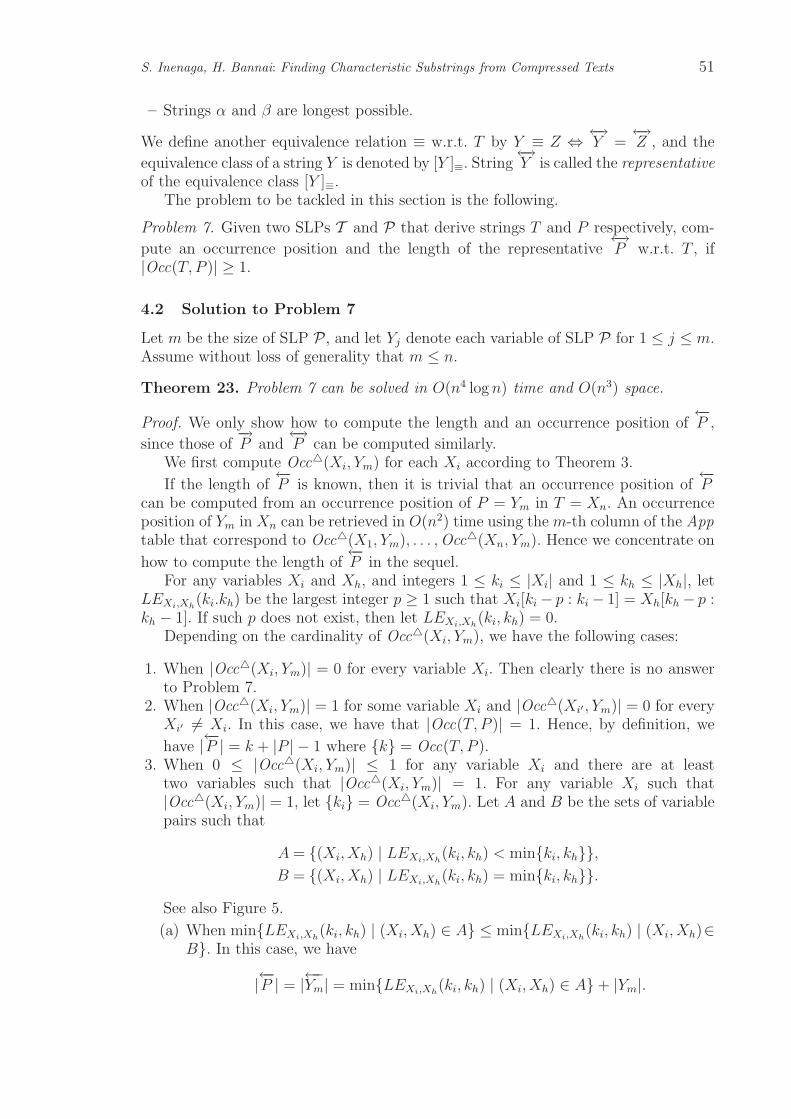
S. Inenaga, H. Bannai: Finding Characteristic Substrings from Compressed Texts 51
– Strings α and β are longest possible.
We define another equivalence relation ≡ w.r.t. T by Y ≡ Z ⇔ ←→Y =←→Z , and the
equivalence class of a string Y is denoted by [Y ]≡. String←→Y is called the representative
of the equivalence class [Y ]≡.The problem to be tackled in this section is the following.
Problem 7. Given two SLPs T and P that derive strings T and P respectively, com-
pute an occurrence position and the length of the representative←→P w.r.t. T , if
|Occ(T, P )| ≥ 1.
4.2 Solution to Problem 7
Let m be the size of SLP P , and let Yj denote each variable of SLP P for 1 ≤ j ≤ m.Assume without loss of generality that m ≤ n.
Theorem 23. Problem 7 can be solved in O(n4 log n) time and O(n3) space.
Proof. We only show how to compute the length and an occurrence position of←−P ,
since those of−→P and
←→P can be computed similarly.
We first compute Occ(Xi, Ym) for each Xi according to Theorem 3.
If the length of←−P is known, then it is trivial that an occurrence position of
←−P
can be computed from an occurrence position of P = Ym in T = Xn. An occurrenceposition of Ym in Xn can be retrieved in O(n2) time using the m-th column of the Apptable that correspond to Occ(X1, Ym), . . . ,Occ(Xn, Ym). Hence we concentrate on
how to compute the length of←−P in the sequel.
For any variables Xi and Xh, and integers 1 ≤ ki ≤ |Xi| and 1 ≤ kh ≤ |Xh|, letLEXi,Xh
(ki.kh) be the largest integer p ≥ 1 such that Xi[ki− p : ki− 1] = Xh[kh− p :kh − 1]. If such p does not exist, then let LEXi,Xh
(ki, kh) = 0.Depending on the cardinality of Occ(Xi, Ym), we have the following cases:
1. When |Occ(Xi, Ym)| = 0 for every variable Xi. Then clearly there is no answerto Problem 7.
2. When |Occ(Xi, Ym)| = 1 for some variable Xi and |Occ(Xi′ , Ym)| = 0 for everyXi′ 6= Xi. In this case, we have that |Occ(T, P )| = 1. Hence, by definition, we
have |←−P | = k + |P | − 1 where k = Occ(T, P ).3. When 0 ≤ |Occ(Xi, Ym)| ≤ 1 for any variable Xi and there are at least
two variables such that |Occ(Xi, Ym)| = 1. For any variable Xi such that|Occ(Xi, Ym)| = 1, let ki = Occ(Xi, Ym). Let A and B be the sets of variablepairs such that
A = (Xi, Xh) | LEXi,Xh(ki, kh) < minki, kh,
B = (Xi, Xh) | LEXi,Xh(ki, kh) = minki, kh.
See also Figure 5.
(a) When minLEXi,Xh(ki, kh) | (Xi, Xh) ∈ A ≤ minLEXi,Xh
(ki, kh) | (Xi, Xh)∈B. In this case, we have
|←−P | = |←−Ym| = minLEXi,Xh(ki, kh) | (Xi, Xh) ∈ A+ |Ym|.

52 Proceedings of the Prague Stringology Conference 2009
Xi
Ym
Xh
ki
kh
Xl(i) Xr(i)
Xl(h) Xr(h)
Xi
Xl(i) Xr(i)
Ym
Xh
Xl(h) Xr(h)
ki
kh
Figure 5. LEXi,Xh(ki, kh) < minki, kh (left) and LEXi,Xh
(ki, kh) = minki, kh(right).
(b) When minLEXi,Xh(ki, kh) | (Xi, Xh) ∈ A > minLEXi,Xh
(ki, kh) | (Xi, Xh)∈B.For any pair of variables Xi, Xh ∈ B, assume w.l.o.g. that ki ≥ kh. Let Xh =Xℓ(h)Xr(h).For any variable Xi such that |Occ(Xi, Ym)| = 1, we compute
Gi = Occ(Xi, Xℓ(h)) ∩ (Occ(Xi, Ym)⊖ kh).
Note that |Gi| ≤ 1, since |Occ(Xi, Ym)| = 1. Let Xi, Xj be any variablessuch that Gi = gi, Gj = gj and gi ≤ gj. We compute LEXi,Xj
(gi, gj) untilLEXi,Xj
(gi, gj) < mingi, gj or Xi is a prefix of T (see Figure 6).i. When minLEXi,Xh
(Ym, ki, kh) | (Xi, Xh) ∈ A ≥ LEXi,Xj(gi, gj). In this
case, LEXi,Xj(gi, gj) + |Ym| is a new candidate for |←−Ym|.
ii. When minLEXi,Xh(Ym, ki, kh) | (Xi, Xh) ∈ A < LEXi,Xj
(gi, gj). In this
case, LEXi,Xj(gi, gj) + |Ym| is not a candidate for |←−Ym|.
4. When 0 ≤ |Occ(Xi, Ym)| ≤ 2 for any 1 ≤ i ≤ n. This case can be solved in asimilar way to Case 3.
5. When |Occ(Xi, Ym)| ≥ 3 for some 1 ≤ i ≤ n. It follows from Lemma 1 thatYm = P = udv where |u| is the smallest period of P , d ≥ 2 is a positive integer,
and v is a proper (possibly empty) prefix of u. It now holds that |←−Ym| < |u|+ |Ym|,since every occurrence of Ym in Occ(Xi, Ym) except for the first one is alwayspreceded by u.
The length of←−Ym can be computed as follows. See also Figure 7. For all variables
Xi = Xℓ(i)Xr(i) such that |Occ(Xi, Ym)| ≥ 1, compute FM (Xℓ(i), Xℓ(i), |u| + 1).Then we have
|←−P | = |←−Ym| = minFM (Xℓ(i), Xℓ(i), |u|+ 1) mod |u| | |Occ(Xi, Ym)| ≥ 1+ |Ym|.Now we analyze the complexity. By Theorem 3, Occ(Xi, Ym) can be computed in
O(n3) time with O(n2) space. Moreover, the cardinality, and a membership query toeach Occ(Xi, Ym) is answered in constant time due to Lemma 1. Therefore, Cases 1and 2 can be solved in constant time provided that Occ(Xi, Ym) are pre-computed.

S. Inenaga, H. Bannai: Finding Characteristic Substrings from Compressed Texts 53
Xi
Ym
Xj
Xl(h)
Xr(j)
gi
gj
Xl(j)
Xl(i) Xr(i)
Figure 6. Compute LEXi,Xj(gi, gj) until LEXi,Xj
(gi, gj) < mingi, gj or Xi is a prefixof T .
Xi
Xl(i) Xr(i)
Ym
uu vu
uu vu
uu vu
uu vuuw
uu vu
Xl(i)
uu vuuw
Xl(i)
uu vuuw
|u|
Figure 7. Illustration for Case 5. String w is a proper suffix of u such that everyoccurrence of Ym = udv is preceded by w (left). The length of w can be computed as|w| = FM (Xℓ(i), Xℓ(i), |u|+ 1) mod |u| (right).
Now consider Case 3. We compute the value of LEXi,Xh(ki, kh) for all pairs of vari-
ables, whose number is O(n2). Since ki = Occ(Xi, Ym) and kh = Occ(Xh, Ym),it holds that
LEXi,Xh(ki, kh) = FM (Xi, Xℓ(h), |Xi| − ki − |Xℓ(h)|+ kj + 1)− |Xℓ(h)|+ kh. (2)
It follows from Lemma 6 that Case 3a can be solved in O(n3 log n) time. Now fo-cus on Case 3b. For any variable Xi, Gi can be computed in O(n) time, since|Occ(Xi, Ym)| = 1 and a membership query to Occ(Xi, Xℓ(h)) can be answeredin O(n) time due to Lemma 2. In each step of the loop, we compute the value ofLEXi,Xj
(gi, gj) + |Ym| for O(n2) pairs of variables. During this loop, the value ofLEXi,Xj
(gi, gj) + |Ym| is monotonically non-decreasing, and the size of Gi is mono-

54 Proceedings of the Prague Stringology Conference 2009
tonically non-increasing. Hence, the depth of the loop is bounded by n. Moreover, wehave that
LEXi,Xj(gi, gj) = FM (Xj, Xℓ(i), |Xi| − kj − |Xℓ(i)|+ ki + 1)− |Xℓ(i)|+ gi. (3)
By Equation (3) and Lemma 6, the total time cost for Case 3b is O(n4 log n). There-fore, Case 3 is solvable in O(n4 log n) time, and so is Case 4.
In Case 5 we call the FM function at most n times, and each call of the FMfunction takes O(n log n) time by Lemma 6. Hence Case 5 can be solved in O(n2 log n)time.
Computing OL(Xi, Xj) for each pair of variables Xi, Xj requires O(n4 log n) timeand O(n3) space due to Theorem 5. Overall, we conclude that Problem 7 can besolved in O(n4 log n) time with O(n3) space. ⊓⊔
References
1. A. Blumer, J. Blumer, D. Haussler, R. Mcconnell, and A. Ehrenfeucht: Completeinverted files for efficient text retrieval and analysis. J. ACM 34(3), 1987, pp. 578–595.
2. R. Feldman and J. Sanger: The Text Mining Handbook: Advanced Approaches in AnalyzingUnstructured Data, Cambridge University Press, 2007.
3. L. Gasieniec, M. Karpinski, W. Plandowski, and W. Rytter: Efficient algorithms forLempel-Ziv encoding, in Proc. 5th Scandinavian Workshop on Algorithm Theory (SWAT’96),vol. 1097 of Lecture Notes in Computer Science, Springer-Verlag, 1996, pp. 392–403.
4. M. Karpinski, W. Rytter, and A. Shinohara: An efficient pattern-matching algorithm forstrings with short descriptions. Nordic Journal of Computing, 4 1997, pp. 172–186.
5. J. Kieffer, E. Yang, G. Nelson, and P. Cosman: Universal lossless compression viamultilevel pattern matching. IEEE Transactions on Information Theory, 46(4) 2000, pp. 1227–1245.
6. Y. Lifshits: Solving classical string problems an compressed texts, in Combinatorial and Al-gorithmic Foundations of Pattern and Association Discovery, no. 06201 in Dagstuhl SeminarProceedings, 2006.
7. Y. Lifshits: Processing compressed texts: A tractability border, in Proc. 18th Annual Sympo-sium on Combinatorial Pattern Matching (CPM’07), vol. 4580 of Lecture Notes in ComputerScience, Springer-Verlag, 2007, pp. 228–240.
8. W. Matsubara, S. Inenaga, A. Ishino, A. Shinohara, T. Nakamura, and
K. Hashimoto: Efficient algorithms to compute compressed longest common substrings andcompressed palindromes. Theoretical Computer Science, 410(8–10) 2009, pp. 900–913.
9. M. Miyazaki, A. Shinohara, and M. Takeda: An improved pattern matching algorithm forstrings in terms of straight-line programs, in Proc. 8th Annual Symposium on CombinatorialPattern Matching (CPM’97), vol. 1264 of Lecture Notes in Computer Science, Springer-Verlag,1997, pp. 1–11.
10. K. Narisawa, H. Bannai, K. Hatano, and M. Takeda: Unsupervised spam detectionbased on string alienness measures, in Proc. 10th International Conference on Discovery Science(DS’07), vol. 4755 of Lecture Notes in Artificial Intelligence, 2007, pp. 161–172.
11. C. G. Nevill-Manning, I. H. Witten, and D. L. Maulsby: Compression by induction ofhierarchical grammars, in Proc. Data Compression Conference ’94 (DCC’94), IEEE ComputerSociety, 1994, pp. 244–253.
12. W. Rytter: Grammar compression, LZ-encodings, and string algorithms with implicit input, inProc. 31st International Colloquium on Automata, Languages and Programming (ICALP’04),vol. 3142 of Lecture Notes in Computer Science, Springer-Verlag, 2004, pp. 15–27.
13. M. Takeda, T. Matsumoto, T. Fukuda, and I. Nanri: Discovering characteristic expres-sions in literary works. Theoretical Computer Science, 292(2) 2003, pp. 525–546.
14. J. Ziv and A. Lempel: A universal algorithm for sequential data compression. IEEE Trans-actions on Information Theory, IT-23(3) 1977, pp. 337–349.
15. J. Ziv and A. Lempel: Compression of individual sequences via variable-length coding. IEEETransactions on Information Theory, 24(5) 1978, pp. 530–536.

Delta Encoding in a Compressed Domain
Shmuel T. Klein and Moti Meir
Department of Computer ScienceBar Ilan University
Ramat Gan 52900, IsraelTel: (972–3) 531 8865 Fax: (972–3) 736 [email protected], [email protected]
Abstract. A delta compression algorithm is presented, working on an LZSS com-pressed reference file and an uncompressed version, and producing a delta file thatcan be used to reconstruct the version file directly in its compressed form. This hasapplications to accelerate data flow in network environments.
1 Introduction
This paper presents an algorithmic approach to work with highly correlated files inthe compressed domain. The idea is to allow small changes to be reflected upon areference file each time a newer file version becomes available. This ability is highlyrequired by caching, versioning and additive backup systems.
The standard delta compression scheme [3,1,4,9,2] takes two files and outputs thedifference between those files. Such a scheme tries to output a small amount of datawhich represents the difference between the two files in their uncompressed state. Asa result, using the standard delta file scheme, one can reconstruct a version file byusing a reference file and the delta file (see Figure 1.a). Our scheme, however, encodesa delta file that reflects the differences between the files in their compressed state.That is, using the delta file and the compressed reference file, the decoder outputs thecompressed version file (See Figure 1.b), contrarily to standard delta schemes thatwould output a version file in uncompressed form. Our scheme uses an uncompressedversion file and a compressed reference file as the inputs to the encoder, a scenariodefined as semi-compressed delta encoding in [7], in contrast with the fully-compressedalternative treated in [6].
We provide a conceptual solution considering the fact that textual data is pro-duced in uncompressed form and also by examination of the entire network routebetween the encoding part (usually a server) and the decoding part (usually a client),which includes intermediate network elements. The scheme considers the fact thatmost of the network’s intermediate elements are indifferent to the data content andonly wish to store and forward the most recent copy of the data. For such elements,having the ability to alter their cached copy without decompressing it first as neededwhen a regular delta encoding is used, presents a great advantage. Standard schemesproducing uncompressed version files would require an encoding phase, that is, com-pressing the file in order to save storage space and network bandwidth. This imposesa penalty in terms of both CPU utilization and temporary storage space, which canbe saved by directly dealing with a compressed output.
The proposed encoding algorithm has two inputs: the compressed reference fileRc, and the uncompressed version file V . The output of the encoder is a delta file∆, which, together with Rc, is the input to the decoding algorithm that outputs thecompressed version file Vc.
Shmuel T. Klein, Moti Meir: Delta Encoding in a Compressed Domain, pp. 55–64.
Proceedings of PSC 2009, Jan Holub and Jan Zd’arek (Eds.), ISBN 978-80-01-04403-2 c© Czech Technical University in Prague, Czech Republic

56 Proceedings of the Prague Stringology Conference 2009
A
B
Encode
Delta (A,B)
Decode A
B
R-Comp
V
Encode
Delta (R,V)
Decode R-Comp
V-Comp
1.a 1.b
Figure 1. Schematic representation of delta encoding
The efficiency of our scheme is based on several assumptions regarding both ver-sion and reference files:
1. The files are highly correlated2. The changes are local and sparse3. The changes are very small compared to the size of V .
The algorithm is an extension of LZSS [5] encoding and uses an ordered hashtable adapted from [10], to store previous occurrences of substrings. The parameterswhich control the encoding are:
– Window size — the length of the sliding window. This attribute defines the maxi-mum valid size of the jumpbacks and thereby the maximum “memory” size of thehash table.
– Minimum Match — determines the minimum number of characters required tomatch, in order to create a back pointer to the previous text.
– Synch Chunk — the maximum number of characters that are affected by a singlechange. That is, the length of all changes are smaller than this number.
The output of the encoder is a set of COPY, ADD, UPDATE and SPLIT commands anda set of characters stored in ∆, acting as a set of control commands to a decoder forchanging Rc. These commands are described in more detail in Section 4 below. Thedecoder uses ∆ and Rc to build an updated compressed file equivalent to Vc. This isdone without decoding Rc but rather by changing it while it is still compressed (seeFigure 1.b)
Let Vcr[i, j] be the substring of Vc with index in the real uncompressed form,that is, the indices i and j refer to the indices of V in their uncompressed form. Forexample, if the 100 first bytes of V are compressed to the first 20 elements of Vc,then we have Vc[1, 20] = Compress(V [1, 100]) = Vcr[1, 100]. This provides a reversemapping between the compressed domain and the uncompressed domain locations.We shall use the same notation when referring to just one character of V or R, thatis Vcr[50] = i is the location in Vc that corresponds to character V [50].

Shmuel T. Klein and Moti Meir: Delta Encoding in a Compressed Domain 57
2 The Encoding Algorithm
2.1 Overview
The algorithm encodes V and iteratively compares the results to Rc. During theprocessing, a sequence of characters and back pointers is generated, and checkedfor matches with Rc. If a mismatch is detected — denote the location of this localmismatch point by LMP — the original LZSS algorithm would output a file thatwill greatly differ from Rc. The result would be two encoded files, which were highlycorrelated when uncompressed, and when compared in the compressed domain loosetheir high resemblance. The current encoding fixes this problem by synchronizingboth files. As a consequence there will be a local synchronization point (LSP) afterwhich the output will match exactly the reference file, up to the next LMP. We assumehere that the distance from LSP to LMP is at least Synch Chunk, otherwise the twochanges are considered as one.
Several types of mismatches need to be addressed:
– one element is a back pointer while the other is a character;– both elements are characters, but different ones;– both elements are back pointers, but their copy length differs;– both elements are back pointers, but their jump back length differs.
Maintaining a Local Reconstructed Buffer (LRB) in combination with the assump-tion of a limited change results in the ability to track the change. At each step, thealgorithm checks whether a substitution, insertion or deletion of characters can ex-plain the change, and continues according to the results by locating the LSPs inthe uncompressed domain. When these points are found, the hash table is updatedaccordingly.
For example, consider the case of inserting a line of text into the version file. TheLRB created by the reference instructions and the version data will match at a pointin the version text which is beyond the inserted change. Since the change is assumedto be relatively small, the number of characters inserted is found by running a loopup to synch chunk size, trying to find this substring in the version file.
In order to compare the new version with the reference, we must be able toreconstruct the original substrings which might be represented by pointers in thereference file. This has led to the need of decoding the reference file in order toreconstruct the original data in the change area of V [7], which is the string startingone element prior to the actual change and ending at most Synch Chunk charactersafter the end of the change. The idea of running from right to left in Rc from elementsprior to LMP, collecting the needed reference data characters, does not work well inmost cases due to the fact that a back pointer in the encoded file can point to anotherback pointer, and so on, creating a chain. In addition to being expensive, this rightto left decoding is not local. Since we want to maintain a local approach whichgreatly decreases memory needs, the semi compressed domain is exploited by usingthe reference characters and pointers to reconstruct the original data in the changearea.
There is, however, one exception to the above. Since we use elements from Rc toreconstruct the reference data using the version data, care has to be taken in thecase of self-pointers, i.e., when the copy length is larger than the offset. Indeed, thepossibility of self-pointers is one of the major features of LZ77 schemes like LZSS,enabling the compression of variable-length repetitive strings; for example, a string

58 Proceedings of the Prague Stringology Conference 2009
of 50 a’s can be compressed as a[offset = 1, length = 49]. The solution is to use thealready reconstructed buffer as a reference for self pointers.
2.2 Substitution
This is the simplest case, e.g., a date field has been updated in the version file. Thefollowing steps are executed, referring to Figure 2:
1. find the actual change size by comparing characters from the LRB and V , boundedby the Synch Chunk parameter;
2. insert a new quarantine zone [K,K + i] to the mismatch list;3. output the relevant commands (split and update pointers) to ∆;4. advance the Rc index to point to the location of the LSP, and also advance the
version index to the same LSP.
Version File indices
Reference File indices
1 2 3 4 5 6 7 … K’… (K+i)’ K+i+1… N
Mismatch point
Difference
Block Next Match
1 2 3 4 5 6 7 … K … (K+i) K+i+1 ...N
Figure 2. Schematic representation of substitution
The algorithm works because skipping over the change in both files and backwardsupdating V to the pre-change state, brings us to a point (LSP) where we just needto synchronize the hash tables. After this synchronization, the encoding process isthe same, hence the output of the encoder are COPY and UPDATE commands up to thenext mismatch. As we can see in Figure 2, jumping in both files as close as possibleto index K + i + 1 will bring us to the LSP. The reason that one does not always getexactly to K + i + 1 is that the exact pointers from Rc are used and they are notsplit. However, breaking the back pointers to get to the exact spot in V is feasibleand could in certain cases result in better compression.
2.3 Insertion
An inserted string may dramatically change the original LZSS output, as shown inFigure 3. V is scanned for an occurrence of the content of LRB inside the definedlimited area, defined to start from K − j up to K + i, where i is the Synch Chunksize and j is the maximum change size. The simplest way to deal with the insertionis to adjoin the inserted block to ∆ with a single ADD and one ADJUST command. Onecould also consider using the hash table to add the newly inserted text as a sequenceof pointers, which might improve compression.
In any case, a set of adjustment commands needs to be added to correct the backpointers of Rc. Each back pointer which points to the index in V prior to LMP hasto be increased by the length of the insertion. If the increased length exceeds themaximum defined, the back pointer is split and the exceeding part is inserted asindividual characters.

Shmuel T. Klein and Moti Meir: Delta Encoding in a Compressed Domain 59
Version File indices
Reference File indices
1 2 3 4 5 6 7 … (K-j)…(K-1) K … (K+i) … N
1 2 3 4 5 6 7 … K … (K+i) … N
Mismatch point
Missing Block
Next Match
Figure 3. Schematic representation of insertion
2.4 Deletion
Deletion is similar to insertion, but here the LRB is scanned for an occurrence of asubstring of V . The steps are, referring to Figure 4:
1. LRB ←− decode(Rc[K,K + i], V )2. search for V [K + j,K + i] in LRB;3. output to ∆ a COPY command up to LMP; if LMP lies within a string compressed
by a pointer, this pointer has to be split or some prefix of this string needs to beinserted by an ADD command;
4. output to ∆ an ADJUST command for [K,K +i] of Rc to reduce the relevant offsetsby the length of the deleted string.
Version File indices
Reference File indices
1 2 3 4 5 6 7 … K+j ... (K+i) … N
Mismatch point
Difference
Block Next Match
1 2 3 4 5 6 7 … K … (K+j-1) (K+j) ... (K+i) … N
Figure 4. Schematic representation of deletion
3 The Decoding Algorithm
The descriptive nature of ∆ is used to apply change commands to Rc, thereby trans-forming it into a file which is equivalent to Vc. The decoding process is linear in timeand storage but is slightly more complex than the original LZSS decoding. This isdue to the fact that pointers need to be adjusted along the way as data is inserted toor deleted from Vc. Moreover, the chain breaking mechanism might result in pointersplitting, as discussed above.

60 Proceedings of the Prague Stringology Conference 2009
The algorithm is as follows, with the SPLITTO3 command explained below:
while ∆ commands exist do:if COPY command
copy substring of Rc to Vc
if ADD commandinsert string into Vc
if ADJUST pointers [i, j]do, up to window size from j + 1
add the change size to the jump value of the pointers thatpoint to a location preceding i;
if the pointer is invalidated, issue a SPLITTO3 commandend do
end ifend while
As can be seen, the decoder runs in linear time and does not require additionalmemory. The algorithm performs a few more passes on parts of the data, but assumingthe input is large relative to the window size, these passes are negligible. Further, ifwe consider a worst case scenario of needing to act upon many pointers pointing tothe changed area, the pointers are bounded by the offset bits allocated for the pointerwhich bounds the entire procedure to part of the data. We assume that this is a smallpart compared to the input size. Again, if the changes are frequent in the input, theresult will be a larger delta file and will require much work in the decoder. In such acase, it might be better to send the entire compressed version file and start fresh.
4 The Delta File
The delta file encapsulates commands which instruct the decoder how to convert itsold compressed reference into a new compressed version. By applying the commandsof the delta file, the decoding algorithm outputs the compressed version file withvery low computational needs. The delta file is constructed such that the decodingcomplexity will be as small as possible and most of the computational effort is doneby the encoder. This policy was chosen in order to be consistent with the hop by hopscheme to which this new compression suits. Reducing the complexity of the decoderin both time and storage allows small or computationally weak caching devices to beone of the hops along the way. Also, since the changes are the result of changes inthe server side, the server can do most of the work for all the hops along the pathto the clients. This will allow better utilization of the network nodes along the pathbetween the server and the clients including the clients themselves.
Most of the previous work on delta files refers to an uncompressed domain, forexample VCDIFF [8]. In our case, one needs in addition to the ADD, COPY and RUN
commands of VCDIFF also means to split a pointer in order to insert changes. Thenew SPLITTO3 command breaks a pointer into three parts: the (possibly empty)prefix represents the pointer to the data portion which did not change; the middlepart represents the change to be inserted and the (again possibly empty) suffix pointsto the representation of the remaining data. This methodology allows us to break thepointers of the compressed file and perform chain breaking with very little effort bythe decoder.

Shmuel T. Klein and Moti Meir: Delta Encoding in a Compressed Domain 61
In order to maintain this idea of lowering the computational demands of thedecoder, we write all needed commands to ∆ such that the decoder algorithm willnot need to trace the restriction zones. This might lead to a larger delta file, but thesize penalty is reasonable when the complexity needed by the hops is lower by doingmost of the chain breaking at the encoder side.
Summarizing, the complete delta file command set consists of:
– COPY — similar to the copy of VCDIFF, it tells the decoder to copy a substringfrom the reference file to the decoded file.
– ADDP — Adds a pointer to Vc. This command is similar to VCDIFF’s ADD command,but adds a pointer, not characters.
– ADDS — Adds a string. Instructs the decoder to embed the command’s parameterstring into Vc in its current index. This command is similar to other delta fileencoding ADD commands.
– SPLITTO3 — the basic pointer breaking technique when a change which is in themiddle of an area covered by a pointer is encountered. The decoder has to replacethe changed pointer so that the result will be a reflection of the change in thecompressed output. We split the pointer into three parts, the prefix part up tothe change, the inserted part, which can be some string or a pointer to an earlyappearance, and a suffix part covering the remainder. The SPLITTO3 commandis also used when the encoder gets to a backpointer which points to a restrictedzone. Since restricted zones need to be ignored as they represent invalid data,the command is used to break these pointers. The encoding algorithm stores eachrestricted zone and detects the first pointers that point to a restricted zone, thensplits them. This way, we apply chain breaking, since, if we have P1 pointing toa point in a restricted zone, and P2 pointing to P1, then by fixing P1 we alsotake care of P2 and the rest of the pointers that are connected to them. Also,this way we remove the decoder’s need to trace pointers to restricted zones, hencesimplifying the decoding algorithm.
– ADJUSTJP — Instructs the decoder to adjust all the offset sizes of the pointers,starting from a given start index up to a window size in Rc.
The size of the delta file is a major factor in the proposed scheme. Imagine a casewhere the compressed version is similar in size to the delta file. This overabundanceof data is not needed since we could have sent Vc instead of the delta file. Sending Vc
results is consuming less resources since there is no need for decoding along the pathin each hop. Therefore, the rule is that if |∆| ≪ |Vc|, send ∆. Otherwise, it is betterto send Vc.
The following is a small sample of ∆ in its textual form. In practice we used abinary code in order to encode the commands. Further, when dealing with very largefiles, in which the delta file is also large enough, ∆ itself can be compressed in orderto further reduce its size.

62 Proceedings of the Prague Stringology Conference 2009
COPY [from = 0, to = 77]SPLITTO3 [offset = 114, length = 113]
PrefixPointer = [offset = 114, length = 103]Change = [’2’] // substitute one characterSuffixPointer = [offset = 9, length = 9]
COPY [from = 81, to = 180]
The sample above represents a ∆ of changing a single character in a file V con-sisting of 2864 1-byte numbers. In this example, a single number 1 has been changedinto the number 2. The original file was compressed using LZSS to become Rc of size180 bytes. The decoder algorithm manipulates Rc using the above ∆ to output Vc.
5 Experiments
Table 1 summarizes the benefits of using the proposed algorithm. Real life HTMLfiles have been used, e.g., www.cnn.com, with uncompressed size of 107 KByte, textfiles such as RFC’s and a set of synthetic files, including many repetitions. The changetype has been restricted in the tests to substitutions (S) and insertions (I), as dele-tions behave symmetrically to insertions. The results are compared to the binaryuncompressed delta encoding scheme XDelta, which uses zlib to compress its deltafile that requires a decompression phase before it can be used to reconstruct theuncompressed version. Our scheme takes into consideration that network elementsare indifferent to the content of the data and thus prefer to maintain cached filesin their compressed form and not to decompress them for running the delta encod-ing algorithm or recompress them after reconstruction. The results are compared tore-encoding the new version data, since this scenario represents a reference imple-mentation of compression based transactions between a client and a server, for bothtypes of regular recompression and the proposed delta encoding.
File Number of Change Change size GZip CDDelta XdeltaChanges type (bits) (bits) (bits) (bits)
CNN 0 No change 0 168472 67 1160CNN 1 S 8 169944 145 1688CNN 1 I 128 170024 265 1808CNN 2 S 48 168496 255 1784CNN 2 I 1608 168744 1912 2408CNN 3 I 1872 168744 2254 2592CNN 4 I 2144 168912 2652 2864CNN 5 I 2408 169088 3042 3032CNN 6 I 2672 169120 3384 3144
synthetic 1 S 8 1960 201 1712synthetic 1 I 24 2136 217 1800synthetic 1 S 72 2016 257 1728
Table 1: Experimental results
The first row of Table 1 describes the case of no change in the version file. Eventhough this case looks odd at first, it is a real life case. When considering the networkelements that cache the data from a server, combined with the HTTP cache controlcommands, we see that many data objects, including textual HTML files, have an

Shmuel T. Klein and Moti Meir: Delta Encoding in a Compressed Domain 63
expiration time. This expiration time causes the caching element to ask the server ifthe data was modified (the if-modified-since HTTP attribute) and in some cases,depending on both the network element and the server type, it causes the networkelement to ask for a new version. In this typical case, our scheme will always outputa 67 bit command which is to copy the entire reference file.
The encoder performance has been tested on an Intel’s core 2 due processor2.4 GHz, and achieved a throughput of 36 MByte/sec on one CPU. This performanceis similar to our LZSS encoder implementation. A 3 bit field was used to representthe command, and 32 bits for an index in the file, such as the from field of the COPY
command. When referring to offsets, as in the ADJUSTP command, 16 bits were used,since the window size was up to 64 Kbytes.
0 10 20 30 40 50 60 70 80 90 1000
1
2
3
4
5
6
7x 10
4
Number of changes
size in bits
Delta file size growth as fuction of changes
up to 120 characters
up to 80 characters
up to 40 characters in one change
Figure 5. Size of delta file as function of the number of changes
From Table 1 we can see that on this data, a factor of about 46 is gained whencompared to the compressed size of the file. The Delta file size increases when thereare more changes. However, changes that were tested reflect a change of 7.4 lineswith an average size of 45 characters per line. It must be noted that these results arewithout compression of the delta file and with no compression of the changed datarelative to itself or relative to the entire file as a reference.
Figure 5 shows the size increase in bits of the delta file as a function of the numberof changes, where each such change affects a randomly chosen set of 40, 80 and 120characters. We can see that the size of the delta file increases linearly with the numberof changes.
Figure 6 visualizes the data included in Table 1 concerning the size relation be-tween a gzip compressed file (CNN) and the Delta file for our insertion tests. Thex-axis gives the number of insertions, and the y -axis the size of the file on a logarith-mic scale. We can see that the Delta file size increases with the number of insertedcharacters, while the insertion has only a negligible effect on the size of the new ver-sion gzip compressed file. The Delta file consists mostly of the inserted charactersthemselves.

64 Proceedings of the Prague Stringology Conference 2009
Figure 6. Comparing Gzip and Delta sizes
6 Conclusion
We focused on the semi-compressed delta encoding problem for LZSS encoded files, inan application in which the reconstructed version file is directly given in compressedform. This can greatly reduce network traffic and the CPU and storage requirements ofthe various network elements. The algorithm is based on a partial local reconstructionof a previous occurrence of the data, using the compressed reference and the newversion.
References
1. M. Ajtai, R. Burns, R. Fagin, D. Long, and L. Stockmeyer: Compactly encodingunstructured input with differential compression. Journal of the ACM, 49(3) 2002, pp. 318–367.
2. B. B. C. Xiao and G. Chang: Delta compression for fast wireless internet download. IEEEGLOBECOM Proceedings, 2005, pp. 474–478.
3. M. Chan and T. Woo: Cache-based compaction: A new technique for optimizing web transfer.Proceedings of the IEEE Infocom ’99 Conference, 1999, pp. 117–125.
4. J. Hunt, K. Vo, and W. Tichy: Delta algorithms: An empirical analysis. ACM Trans. onSoftware Eng. and Methodology, 7(2) 1998, pp. 192–214.
5. J. Storer and T. Syzmanski: Data compression via textual substitution. Journal of theACM, 29 1982, pp. 928–951.
6. S. Klein, T. Serebro, and D. Shapira: Modeling delta encoding of compressed files. Inter-national Journal of the Foundations of Computer Science, 19 2008, pp. 137–146.
7. S. Klein and D. Shapira: Compressed delta encoding for LZSS encoded files. Proceedings ofData Compression Conference, DCC–07, 2007, pp. 113–122.
8. D. Korn, J. MacDonald, J. Mogul, and K. Vo: The VCDIFF Generic Differencing andCompression Data Format. RFC 3284 (Proposed Standard), June 2002.
9. G. Motta, J. Gustafson, and S. Chen: Differencial compression of executable code. Pro-ceedings of Data Compression Conference, DCC–07, 2007, pp. 103–112.
10. R. Williams: An extremly fast Ziv-Lempel data compression algorithm. Proceedings of DataCompression Conference, DCC–91, 1991, pp. 362–371.

On Bijective Variants of the
Burrows-Wheeler Transform
Manfred Kufleitner
Universitat Stuttgart, FMI,Universitatsstr. 38, 70569 Stuttgart, Germany
Abstract. The sort transform (ST) is a modification of the Burrows-Wheeler trans-form (BWT). Both transformations map an arbitrary word of length n to a pair con-sisting of a word of length n and an index between 1 and n. The BWT sorts all rotationconjugates of the input word, whereas the ST of order k only uses the first k lettersfor sorting all such conjugates. If two conjugates start with the same prefix of lengthk, then the indices of the rotations are used for tie-breaking. Both transforms outputthe sequence of the last letters of the sorted list and the index of the input within thesorted list. In this paper, we discuss a bijective variant of the BWT (due to Scott),proving its correctness and relations to other results due to Gessel and Reutenauer(1993) and Crochemore, Desarmenien, and Perrin (2005). Further, we present a novelbijective variant of the ST.
1 Introduction
The Burrows-Wheeler transform (BWT) is a widely used preprocessing techniquein lossless data compression [5]. It brings every word into a form which is likely tobe easier to compress [18]. Its compression performance is almost as good as PPM(prediction by partial matching) schemes [7] while its speed is comparable to thatof Lempel-Ziv algorithms [13,14]. Therefore, BWT based compression schemes are avery reasonable trade-off between running time and compression ratio.
In the classic setting, the BWT maps a word of length n to a word of length n andan index (comprising O(log n) bits). Thus, the BWT is not bijective and hence, itis introducing new redundancies to the data, which is cumbersome and undesired inapplications of data compression or cryptography. Instead of using an index, a verycommon technique is to assume that the input has a unique end-of-string symbol[3,18]. Even though this often simplifies proofs or allows speeding up the algorithms,the use of an end-of-string symbol introduces new redundancies (again O(log n) bitsare required for coding the end-of-string symbol).
We discuss bijective versions of the BWT which are one-to-one correspondencesbetween words of length n. In particular, no index and no end-of-string symbol isneeded. Not only does bijectivity save a few bits, for example, it also increases datasecurity when cryptographic procedures are involved; it is more natural and it canhelp us to understand the BWT even better. Moreover, the bijective variants giveus new possibilities for enhancements; for example, in the bijective BWT differentorders on the letters can be used for the two main stages.
Several variants of the BWT have been introduced [2,17]. An overview can befound in the textbook by Adjeroh, Bell, and Mukherjee [1]. One particularly importantvariant for this paper is the sort transform (ST), which is also known under the nameSchindler transform [22]. In the original paper, the inverse of the ST is described only
Manfred Kufleitner: On Bijective Variants of the Burrows-Wheeler Transform, pp. 65–79.
Proceedings of PSC 2009, Jan Holub and Jan Zd’arek (Eds.), ISBN 978-80-01-04403-2 c© Czech Technical University in Prague, Czech Republic

66 Proceedings of the Prague Stringology Conference 2009
very briefly. More precise descriptions and improved algorithms for the inverse of theST have been proposed recently [19,20,21]. As for the BWT, the ST also involves anindex or an end-of-string symbol. In particular, the ST is not onto and it introducesnew redundancies.
The bijective BWT was discovered and first described by Scott (2007), but hisexposition of the algorithm was somewhat cryptic, and was not appreciated as such.In particular, the fact that this transform is based on the Lyndon factorization wentunnoticed by Scott. Gil and Scott [12] provided an accessible description of the algo-rithm. Here, we give an alternative description, a proof of its correctness, and moreimportantly, draw connections between Scott’s algorithm and other results in combi-natorics on words. Further, this variation of the BWT is used to introduce techniqueswhich are employed at the bijective sort transform, which makes the main contribu-tion of this paper. The forward transform of the bijective ST is rather easy, but wehave to be very careful with some details. Compared with the inverse of the bijectiveBWT, the inverse of the bijective ST is more involved.
Outline. The paper is organized as follows. In Section 2 we fix some notationand repeat basic facts about combinatorics on words. On our way to the bijectivesort transform (Section 6) we investigate the BWT (Section 3), the bijective BWT(Section 4), and the sort transform (Section 5). We give full constructive proofs forthe injectivity of the respective transforms. Each section ends with a running examplewhich illustrates the respective concepts. Apart from basic combinatorics on words,the paper is completely self-contained.
2 Preliminaries
Throughout this paper we fix the finite non-empty alphabet Σ and assume that Σis equipped with a linear order ≤. A word is a sequence a1 · · · an of letters ai ∈ Σ,1 ≤ i ≤ n. The set of all such sequences is denoted by Σ∗; it is the free monoid over Σwith concatenation as composition and with the empty word ε as neutral element.The set Σ+ = Σ∗ \ε consists of all non-empty words. For words u, v we write u ≤ vif u = v or if u is lexicographically smaller than v with respect to the order ≤ on theletters. Let w = a1 · · · an ∈ Σ+ be a non-empty word with letters ai ∈ Σ. The lengthof w, denoted by |w|, is n. The empty word is the unique word of length 0. We canthink of w as a labeled linear order: position i of w is labeled by ai ∈ Σ and in thiscase we write λw(i) = ai, so each word w induces a labeling function λw. The firstletter a1 of w is denoted by first(w) while the last letter an is denoted by last(w).The reversal of a word w is w = an · · · a1. We say that two words u, v are conjugateif u = st and v = ts for some words s, t, i.e., u and v are cyclic shifts of one another.The j-fold concatenation of w with itself is denoted by wj. A word u is a root of wif w = uj for some j ∈ N. A word w is primitive if w = uj implies j = 1 and henceu = w, i.e., w has only the trivial root w.
The right-shift of w = a1 · · · an is r(w) = ana1 · · · an−1 and the i-fold rightshift ri(w) is defined inductively by r0(w) = w and ri+1(w) = r(ri(w)). We haveri(w) = an−i+1 · · · ana1 · · · an−i for 0 ≤ i < n. The word ri(w) is also well-definedfor i ≥ n and then ri(w) = rj(w) where j = i mod n. We define the ordered con-jugacy class of a word w ∈ Σn as [w] = (w1, . . . , wn) where wi = ri−1(w). It isconvenient to think of [w] as a cycle of length n with a pointer to a distinguished

Manfred Kufleitner: On Bijective Variants of the Burrows-Wheeler Transform 67
starting position. Every position i, 1 ≤ i ≤ n, on this cycle is labeled by ai. In par-ticular, a1 is a successor of an on this cycle since the position 1 is a successor of theposition n. The mapping r moves the pointer to its predecessor. The (unordered)conjugacy class of w is the multiset w1, . . . , wn. Whenever there is no confusion,then by abuse of notation we also write [w] to denote the (unordered) conjugacyclass of w. For instance, this is the case if w is in some way distinguished within itsconjugacy class, which is true if w is a Lyndon word. A Lyndon word is a non-emptyword which is the unique lexicographic minimal element within its conjugacy class.More formally, let [w] = (w,w2, . . . , wn), then w ∈ Σ+ is a Lyndon word if w < wi
for all i ∈ 2, . . . , n. Lyndon words have a lot of nice properties [15]. For instance,Lyndon words are primitive. Another interesting fact is the following.
Fact 1 (Chen, Fox, and Lyndon [6]). Every word w ∈ Σ+ has a unique factor-ization w = vs · · · v1 such that v1 ≤ · · · ≤ vs is a non-decreasing sequence of Lyndonwords.
An alternative formulation of the above fact is that every word w has a uniquefactorization w = vns
s · · · vn11 where ni ≥ 1 for all i and where v1 < · · · < vs is a
strictly increasing sequence of Lyndon words. The factorization of w as in Fact 1 iscalled the Lyndon factorization of w. It can be computed in linear time using Duval’salgorithm [9].
Suppose we are given a multiset V = v1, . . . , vs of Lyndon words enumeratedin non-decreasing order v1 ≤ · · · ≤ vs. Now, V uniquely determines the word w =vs · · · v1. Therefore, the Lyndon factorization induces a one-to-one correspondencebetween arbitrary words of length n and multisets of Lyndon words of total length n.Of course, by definition of Lyndon words, the multiset v1, . . . , vs of Lyndon wordsand the multiset [v1], . . . , [vs] of conjugacy classes of Lyndon words are also inone-to-one correspondence.
We extend the order ≤ on Σ as follows to non-empty words. Let wω = www · · ·be the infinite sequences obtained as the infinite power of w. For u, v ∈ Σ+ wewrite u ≤ω v if either uω = vω or uω = paq and vω = pbr for p ∈ Σ∗, a, b ∈ Σwith a < b, and infinite sequences q, r; phrased differently, u ≤ω v means that theinfinite sequences uω and vω satisfy uω ≤ vω. If u and v have the same length, then≤ω coincides with the lexicographic order induced by the order on the letters. Forarbitrary words, ≤ω is only a preorder since for example u ≤ω uu and uu ≤ω u. Onthe other hand, if u ≤ω v and v ≤ω u then u|v| = v|u|. Hence, by the periodicitylemma [10], there exists a common root p ∈ Σ+ and g, h ∈ N such that u = pg andv = ph. Also note that b ≤ ba whereas ba ≤ω b for a < b.
Intuitively, the context of order k of w is the sequence of the first k letters of w.We want this notion to be well-defined even if |w| < k. To this end let contextk(w)be the prefix of length k of wω, i.e., contextk(w) consists of the first k letters on thecycle [w]. Note that our definition of a context of order k is left-right symmetric to thecorresponding notion used in data compression. This is due to the fact that typicalcompression schemes are applying the BWT or the ST to the reversal of the input.
An important construction in this paper is the standard permutation πw on theset of positions 1, . . . , n induced by a word w = a1 · · · an ∈ Σn [11]. The first stepis to introduce a new order ¹ on the positions of w by sorting the letters within wsuch that identical letters preserve their order. More formally, the linear order ¹ on1, . . . , n is defined as follows: i ¹ j if
ai < aj or ai = aj and i ≤ j.

68 Proceedings of the Prague Stringology Conference 2009
1 b c b c c b c b c a b b a a b a2 a b c b c c b c b c a b b a a b3 b a b c b c c b c b c a b b a a4 a b a b c b c c b c b c a b b a5 a a b a b c b c c b c b c a b b6 b a a b a b c b c c b c b c a b7 b b a a b a b c b c c b c b c a8 a b b a a b a b c b c c b c b c9 c a b b a a b a b c b c c b c b
10 b c a b b a a b a b c b c c b c11 c b c a b b a a b a b c b c c b12 b c b c a b b a a b a b c b c c13 c b c b c a b b a a b a b c b c14 c c b c b c a b b a a b a b c b15 b c c b c b c a b b a a b a b c16 c b c c b c b c a b b a a b a b
(a) Conjugacy class [w]
5 a a b a b c b c c b c b c a b b4 a b a b c b c c b c b c a b b a8 a b b a a b a b c b c c b c b c2 a b c b c c b c b c a b b a a b6 b a a b a b c b c c b c b c a b3 b a b c b c c b c b c a b b a a7 b b a a b a b c b c c b c b c a
10 b c a b b a a b a b c b c c b c12 b c b c a b b a a b a b c b c c1 b c b c c b c b c a b b a a b a
15 b c c b c b c a b b a a b a b c9 c a b b a a b a b c b c c b c b
11 c b c a b b a a b a b c b c c b13 c b c b c a b b a a b a b c b c16 c b c c b c b c a b b a a b a b14 c c b c b c a b b a a b a b c b
(b) Lexicographically sorted
5 a a b a b c b c c b c b c a b b2 a b c b c c b c b c a b b a a b4 a b a b c b c c b c b c a b b a8 a b b a a b a b c b c c b c b c3 b a b c b c c b c b c a b b a a6 b a a b a b c b c c b c b c a b7 b b a a b a b c b c c b c b c a1 b c b c c b c b c a b b a a b a
10 b c a b b a a b a b c b c c b c12 b c b c a b b a a b a b c b c c15 b c c b c b c a b b a a b a b c9 c a b b a a b a b c b c c b c b
11 c b c a b b a a b a b c b c c b13 c b c b c a b b a a b a b c b c16 c b c c b c b c a b b a a b a b14 c c b c b c a b b a a b a b c b(c) Sorted by 2-order contexts
Figure 1. Computing the BWT and the ST of the word w = bcbccbcbcabbaaba
Let j1 ≺ · · · ≺ jn be the linearization of 1, . . . , n according to this new order. Now,the standard permutation πw is defined by πw(i) = ji.
Example 2. Consider the word w = bcbccbcbcabbaaba over the ordered alphabet a <b < c. We have |w| = 16. Therefore, the positions in w are 1, . . . , 16. For instance,the label of position 6 is λw(6) = b. Its Lyndon factorization is w = bcbcc · bc · bc ·abb · aab · a. The context of order 7 of the prefix bcbcc of length 5 is bcbccbc and thecontext of order 7 of the factor bc is bcbcbcb. For computing the standard permutationwe write w column-wise, add positions, and then sort the pairs lexicographically:
word w w with positions sortedb (b, 1) (a, 10)c (c, 2) (a, 13)b (b, 3) (a, 14)c (c, 4) (a, 16)c (c, 5) (b, 1)b (b, 6) (b, 3)c (c, 7) (b, 6)b (b, 8) (b, 8)c (c, 9) (b, 11)a (a, 10) (b, 12)b (b, 11) (b, 15)b (b, 12) (c, 2)a (a, 13) (c, 4)a (a, 14) (c, 5)b (b, 15) (c, 7)a (a, 16) (c, 9)
This yields the standard permutation
πw =
(1 2 3 4 5 6 7 8 9 10 11 12 13 14 15 1610 13 14 16 1 3 6 8 11 12 15 2 4 5 7 9
).
The conjugacy class [w] of w is depicted in Figure 1(a); the i-th word in [w] is writtenin the i-th row. The last column of the matrix for [w] is the reversal w of w.
3 The Burrows-Wheeler transform
The Burrows-Wheeler transform (BWT) maps words w of length n to pairs (L, i)where L is a word of length n and i is an index in 1, . . . , n. The word L is usually

Manfred Kufleitner: On Bijective Variants of the Burrows-Wheeler Transform 69
referred to as the Burrows-Wheeler transform of w. In particular, the BWT is notsurjective. We will see below how the BWT works and that it is one-to-one. It followsthat only a fraction of 1/n of all possible pairs (L, i) appears as an image under theBWT. For instance (bacd, 1) where a < b < c < d is not an image under the BWT.
For w ∈ Σ+ we define M(w) = (w1, . . . , wn) where w1, . . . , wn = [w] andw1 ≤ · · · ≤ wn. Now, the Burrows-Wheeler transform of w consists of the wordBWT(w) = last(w1) · · · last(wn) and an index i such that w = wi. Note that incontrast to the usual definition of the BWT, we are using right shifts; at this pointthis makes no difference but it unifies the presentation of succeeding transforms. Atfirst glance, it is surprising that one can reconstruct M(w) from BWT(w). Moreover,if we know the index i of w in the sorted list M(w), then we can reconstruct w fromBWT(w). One way of how to reconstruct M(w) is presented in the following lemma.For later use, we prove a more general statement than needed for computing theinverse of the BWT.
Lemma 3. Let k ∈ N. Let⋃s
i=1 [vi] = w1, . . . , wn ⊆ Σ+ be a multiset builtfrom conjugacy classes [vi]. Let M = (w1, . . . , wn) satisfy contextk(w1) ≤ · · · ≤contextk(wn) and let L = last(w1) · · · last(wn) be the sequence of the last symbols.Then
contextk(wi) = λLπL(i) · λLπ2L(i) · · · λLπk
L(i)
where πtL denotes the t-fold application of πL and λLπt
L(i) = λL
(πt
L(i)).
Proof. By induction over the context length t, we prove that for all i ∈ 1, . . . , nwe have contextt(wi) = λLπL(i) · · · λLπt
L(i). For t = 0 we have context0(wi) = ε andhence, the claim is trivially true. Let now 0 < t ≤ k. By the induction hypothesis,the (t − 1)-order context of each wi is λLπL(i) · · ·λLπt−1
L (i). By applying one right-shift, we see that the t-order context of r(wi) is λL(i) · λLπ1
L(i) · · ·λLπt−1L (i).
The list M meets the sort order induced by k-order contexts. In particular,(w1, . . . , wn) is sorted by (t− 1)-order contexts. Let (u1, . . . , un) be a stable sort by t-order contexts of the right-shifts (r(w1), . . . , r(wn)). The construction of (u1, . . . , un)only requires a sorting of the first letters of (r(w1), . . . , r(wn)) such that identicalletters preserve their order. The sequence of first letters of the words r(w1), . . . , r(wn)is exactly L. By construction of πL, it follows that (u1, . . . , un) = (wπL(1), . . . , wπL(n)).Since M is built from conjugacy classes, the multisets of elements occurring in(w1, . . . , wn) and (r(w1), . . . , r(wn)) are identical. The same holds for the multisetsinduced by (w1, . . . , wn) and (u1, . . . , un). Therefore, the sequences of t-order contextsinduced by (w1, . . . wn) and (u1, . . . , un) are identical. Moreover, we conclude
contextt(wi) = contextt(ui) = contextt(wπL(i)) = λLπL(i) · λLπ2L(i) · · · λLπt
L(i)
which completes the induction. We note that in general ui 6= wi since the sort orderof M beyond k-order contexts is arbitrary. Moreover, for t = k + 1 the propertycontextt(wi) = contextt(ui) does not need to hold (even though the multisets of(k + 1)-order contexts coincide). ⊓⊔
Note that in Lemma 3 we do not require that all vi have the same length. Applyingthe BWT to conjugacy classes of words with different lengths has also been used forthe Extended BWT [17].
Corollary 4. The BWT is invertible, i.e., given (BWT(w), i) where i is the indexof w in M(w) one can reconstruct the word w.

70 Proceedings of the Prague Stringology Conference 2009
Proof. We set k = |w|. Let M = M(w) and L = BWT(w). Now, by Lemma 3 we seethat
w = wi = contextk(wi) = λLπ1L(i) · · ·λLπ
|L|L (i).
In particular, w = λLπ1L(i) · · ·λLπ
|L|L (i) only depends on L and i. ⊓⊔
Remark 5. In the special case of the BWT it is possible to compute the i-th elementwi of M(w) by using the inverse π−1
L of the permutation πL:
wi = λLπ−|wi|+1L (i) · · ·λLπ−1
L (i)λL(i).
This justifies the usual way of computing the inverse of (BWT(w), i) from right to left(by using the restriction of π−1
L to the cycle containing the element i). The motivationis that the (required cycle of the) inverse π−1
L seems to be easier to compute than thestandard permutation πL.
Example 6. We compute the BWT of w = bcbccbcbcabbaaba from Example 2. Thelexicographically sorted list M(w) can be found in Figure 1(b). This yields the trans-form (BWT(w), i) = (bacbbaaccacbbcbb, 10) where L = BWT(w) is the last column ofthe matrix M(w) and w is the i-th row in M(w). The standard permutation of L is
πL =
(1 2 3 4 5 6 7 8 9 10 11 12 13 14 15 162 6 7 10 1 4 5 12 13 15 16 3 8 9 11 14
).
Now, π1L(10) · · · π16
L (10) gives us the following sequence of positions starting withπL(10) = 15:
15πL7→ 11
πL7→ 16πL7→ 14
πL7→ 9πL7→ 13
πL7→ 8πL7→ 12
πL7→ 3πL7→ 7
πL7→ 5πL7→ 1
πL7→ 2πL7→ 6
πL7→ 4πL7→ 10.
Applying the labeling function λL to this sequence of positions yields
λL(15)λL(11)λL(16)λL(14)λL(9)λL(13)λL(8)λL(12)
· λL(3)λL(7)λL(5)λL(1)λL(2)λL(6)λL(4)λL(10)
= bcbccbcbcabbaaba = w,
i.e., we have successfully reconstructed the input w from (BWT(w), i).
4 The bijective Burrows-Wheeler transform
Now we are ready to give a comprehensive description of Scott’s bijective variant of theBWT and to prove its correctness. It maps a word of length n to a word of length n—without any index or end-of-string symbol being involved. The key ingredient is theLyndon factorization: Suppose we are computing the BWT of a Lyndon word v, thenwe do not need an index since we know that v is the first element of the list M(v).This leads to the computation of a multi-word BWT of the Lyndon factors of theinput.
The bijective BWT of a word w of length n is defined as follows. Let w = vs · · · v1
with vs ≥ · · · ≥ v1 be the Lyndon factorization of w. Let LM(w) = (u1, . . . , un) whereu1 ≤ω · · · ≤ω un and where the multiset u1, . . . , un =
⋃si=1[vi]. Then, the bijective
BWT of w is BWTS(w) = last(u1) · · · last(un). The S in BWTS is for Scottified. Notethat if w is a power of a Lyndon word, then BWTS(w) = BWT(w).

Manfred Kufleitner: On Bijective Variants of the Burrows-Wheeler Transform 71
In some sense, the bijective BWT can be thought of as the composition of theLyndon factorization [6] with the inverse of the Gessel-Reutenauer transform [11].In particular, a first step towards a bijective BWT can be found in a 1993 articleby Gessel and Reutenauer [11] (prior to the publication of the BWT [5]). The linkbetween the Gessel-Reutenauer transform and the BWT was pointed out later byCrochemore et al. [8]. A similar approach as in the bijective BWT has been employedby Mantaci et al. [16]; instead of the Lyndon factorization they used a decompositionof the input into blocks of equal length. The output of this variant is a word and asequence of indices (one for each block). In its current form, the bijective BWT hasbeen proposed by Scott [23] in a newsgroup posting in 2007. Gil and Scott gave anaccessible version of the transform, an independent proof of its correctness, and theytested its performance in data compression [12]. The outcome of these tests is thatthe bijective BWT beats the usual BWT on almost all files of the Calgary Corpus[4] by at least a few hundred bytes which exceeds the gain of just saving the rotationindex.
Lemma 7. Let w = vs · · · v1 with vs ≥ · · · ≥ v1 be the Lyndon factorization of w,let LM(w) = (u1, . . . , un), and let L = BWTS(w). Consider the cycle C of thepermutation πL which contains the element 1 and let d be the length of C. ThenλLπ1
L(1) · · ·λLπdL(1) = v1.
Proof. By Lemma 3 we see that(λLπ1
L(1) · · ·λLπdL(1)
)|v1| = vd1 . Since v1 is primi-
tive it follows λLπ1L(1) · · ·λLπd
L(1) = vz1 for some z ∈ N. In particular, the Lyndon
factorization of w ends with vz1.
Let U be the subsequence of LM(w) which consists of those ui which come fromthis last factor vz
1. The sequence U contains each right-shift of v1 exactly z times.Moreover, the sort-order within U depends only on |v1|-order contexts.
The element v1 = u1 is the first element in U since v1 is a Lyndon word. Inparticular, π0
L(1) = 1 is the first occurrence of r0(v1) = v1 within U . Suppose πjL(1)
is the first occurrence of rj(v1) within U . Let πjL(1) = i1 < · · · < iz be the indices of
all occurrences of rj(v1) in U . By construction of πL, we have πL(i1) < · · · < πL(iz)and therefore πj+1
L (1) is the first occurrence of rj+1(v1) within U . Inductively, πjL(1)
always refers to the first occurrence of rj(v1) within U (for all j ∈ N). In particular
it follows that π|v1|L (1) = 1 and z = 1. ⊓⊔
Theorem 8. The bijective BWT is invertible, i.e., given BWTS(w) one can recon-struct the word w.
Proof. Let L = BWTS(w) and let w = vs · · · v1 with vs ≥ · · · ≥ v1 be the Lyndonfactorization of w. Each permutation admits a cycle structure. We decompose thestandard permutation πL into cycles C1, . . . , Ct. Let ij be the smallest element of thecycle Cj and let dj be the length of Cj. We can assume that 1 = i1 < · · · < it.
We claim that t = s, dj = |vj|, and λLπ1L(ij) · · ·λLπ
dj
L (ij) = vj. By Lemma 7
we have λLπ1L(i1) · · ·λLπd1
L (i1) = v1. Let π′L denote the restriction of πL to the set
C = C2 ∪ · · · ∪ Ct, where by abuse of notation C2 ∪ · · · ∪ Ct denotes the set of allelements occurring in C2, . . . , Ct. Let L′ = BWTS(vs · · · v2). The word L′ can beobtained from L by removing all positions occurring in the cycle C1. This yields amonotone bijection
α : C → 1, . . . , |L′|

72 Proceedings of the Prague Stringology Conference 2009
such that λL(i) = λL′α(i) and απL(i) = πL′α(i) for all i ∈ C. In particular, πL′ hasthe same cycle structure as π′
L and 1 = α(i2) < · · · < α(it) is the sequence of theminimal elements within the cycles. By induction on the number of Lyndon factors,
vs · · · v2 = λL′π1L′α(it) · · ·λL′πdt
L′α(it) · · · λL′π1L′α(i2) · · ·λL′πd2
L′ (i2)
= λL′απ1L(it) · · ·λL′απdt
L (it) · · · λL′απ1L(i2) · · ·λL′απd2
L (i2)
= λLπ1L(it) · · ·λLπdt
L (it) · · · λLπ1L(i2) · · ·λLπd2
L (i2).
Appending λLπ1L(i1) · · ·λLπd1
L (i1) = v1 to the last line allows us to reconstruct w by
w = λLπ1L(it) · · ·λLπdt
L (it) · · · λLπ1L(i1) · · ·λLπd1
L (i1).
Moreover, t = s and dj = |vj|. We note that this formula for w only depends on Land does not require any index to an element in LM(w). ⊓⊔
Example 9. We again consider the word w = bcbccbcbcabbaaba from Example 2 andits Lyndon factorization w = v6 · · · v1 where v6 = bcbcc, v5 = bc, v4 = bc, v3 = abb,v2 = aab, and v1 = a. The lists ([v1], . . . , [v6]) and LM(w) are:
([v1], . . . , [v6])1 a2 a a b3 b a a4 a b a5 a b b6 b a b7 b b a8 b c9 c b
10 b c11 c b12 b c b c c13 c b c b c14 c c b c b15 b c c b c16 c b c c b
LM(w)1 a2 a a b4 a b a5 a b b3 b a a6 b a b7 b b a8 b c
10 b c12 b c b c c15 b c c b c9 c b
11 c b13 c b c b c16 c b c c b14 c c b c b
Hence, we obtain L = BWTS(w) = abababaccccbbcbb as the sequence of the lastsymbols of the words in LM(w). The standard permutation πL induced by L is
πL =
(1 2 3 4 5 6 7 8 9 10 11 12 13 14 15 161 3 5 7 2 4 6 12 13 15 16 8 9 10 11 14
)
The cycles of πL arranged by their smallest elements are C1 = (1), C2 = (2, 3, 5),C3 = (4, 7, 6), C4 = (8, 12), C5 = (9, 13), and C6 = (10, 15, 11, 16, 14). Applyingthe labeling function λL to the cycle Ci (starting with the second element) yieldsthe Lyndon factor vi. With this procedure, we reconstructed w = v6 · · · v1 from L =BWTS(w).
5 The sort transform
The sort transform (ST) is a BWT where we only sort the conjugates of the inputup to a given depth k and then we are using the index of the conjugates as a tie-breaker. Depending on the depth k and the implementation details this can speed upcompression (while at the same time slightly slowing down decompression).

Manfred Kufleitner: On Bijective Variants of the Burrows-Wheeler Transform 73
In contrast to the usual presentation of the ST, we are using right shifts. Thisdefines a slightly different version of the ST. The effect is that the order of thesymbols occurring in some particular context is reversed. This makes sense, becausein data compression the ST is applied to the reversal of a word. Hence, in the STof the reversal of w the order of the symbols in some particular context is the sameas in w. More formally, suppose w = x0ca1x1ca2x2 · · · casxs for c ∈ Σ+ then in thesort transform of order |c| of w, the order of the occurrences of the letters ai is notchanged. This property can enable better compression ratios on certain data.
While the standard permutation is induced by a sequence of letters (i.e., a word)we now generalize this concept to sequences of words. For a list of non-empty wordsV = (v1, . . . , vn) we now define the k-order standard permutation νk,V induced by V .As for the standard permutation, the first step is the construction of a new linearorder ¹ on 1, . . . , n. We define i ¹ j by the condition
contextk(vi) < contextk(vj) or contextk(vi) = contextk(vj) and i ≤ j.
Let j1 ≺ · · · ≺ jn be the linearization of 1, . . . , n according to this new order. Theidea is that we sort the line numbers of v1, . . . , vn by first considering the k-ordercontexts and, if these are equal, then use the line numbers as tie-breaker. As before,the linearization according to ¹ induces a permutation νk,V by setting νk,V (i) = ji.Now, νk,V (i) is the position of vi if we are sorting V by k-order context such thatthe line numbers serve as tie-breaker. We set Mk(v1, . . . , vn) = (w1, . . . , wn) wherewi = vνk,V (i). Now, we are ready to define the sort transform of order k of a word w:Let Mk([w]) = (w1, . . . , wn); then STk(w) = last(w1) · · · last(wn), i.e., we first sortall cyclic right-shifts of w by their k-order contexts (by using a stable sort method)and then we take the sequence of last symbols according to this new sort order as theimage under STk. Since the tie-breaker relies on right-shifts, we have ST0(w) = w, i.e.,ST0 is the reversal mapping. The k-order sort transform of w is the pair (STk(w), i)where i is the index of w in Mk([w]). As for the BWT, we see that the k-order sorttransform is not bijective.
Next, we show that it is possible to reconstruct Mk([w]) from STk(w). Hence,it is possible to reconstruct w from the pair (STk(w), i) where i is the index of win Mk([w]). The presentation of the back transform is as follows. First, we will in-troduce the k-order context graph Gk and we will show that it is possible to re-build Mk([w]) from Gk. Then we will show how to construct Gk from STk(w). Again,the approach will be slightly more general than required at the moment; but we willbe able to reuse it in the presentation of a bijective ST.
Let V = ([u1], . . . , [us]) = (v1, . . . , vn) be a list of words built from conjugacyclasses [ui] of non-empty words ui. Let M = (w1, . . . , wn) be an arbitrary per-mutation of the elements in V . We are now describing the edge-labeled directedgraph Gk(M) – the k-order context graph of M – which will be used later as a pre-sentation tool for the inverses of the ST and the bijective ST. The vertices of Gk(M)consist of all k-order contexts contextk(w) of words w occurring in M . We draw anedge (c1, i, c2) from context c1 to context c2 labeled by i if c1 = contextk(wi) andc2 = contextk(r(wi)). Hence, every index i ∈ 1, . . . , n of M defines a unique edgein Gk(M). We can also think of last(wi) as an additional implicit label of the edge(c1, i, c2), since c2 = contextk(last(wi)c1).
A configuration (C, c) of the k-order context graph Gk(M) consists of a subset ofthe edges C and a vertex c. The idea is that (starting at context c) we are walking

74 Proceedings of the Prague Stringology Conference 2009
along the edges of Gk(M) and whenever an edge is used, it is removed from the setof edges C. We now define the transition
(C1, c1)u→ (C2, c2)
from a configuration (C1, c1) to another configuration (C2, c2) with output u ∈ Σ∗
more formally. If there exists an edge in C1 starting at c1 and if (c1, i, c2) ∈ C1 isthe unique edge with the smallest label i starting at c1, then we have the single-steptransition
(C1, c1)a→ (C1 \ (c1, i, c2) , c2) where a = last(wi)
If there is no edge in C1 starting at c1, then the outcome of (C1, c1)→ is undefined.
Inductively, we define (C1, c1)ε→ (C1, c1) and for a ∈ Σ and u ∈ Σ∗ we have
(C1, c1)au→ (C2, c2) if (C1, c1)
u→ (C′, c′) and (C′, c′) a→ (C2, c2)
for some configuration (C′, c′). Hence, the reversal au is the label along the path of
length |au| starting at configuration (C1, c1). In particular, if (C1, c1)u→ (C2, c2) holds,
then it is possible to chase at least |u| transitions starting at (C1, c1); vice versa, if weare chasing ℓ transitions then we obtain a word of length ℓ as a label. We note thatsuccessively taking the edge with the smallest label comes from the use of right-shifts.If we had used left-shifts we would have needed to chase largest edges for the followinglemma to hold. The reverse labeling of the big-step transitions is motivated by thereconstruction procedure which will work from right to left.
Lemma 10. Let k ∈ N, V = ([v1], . . . , [vs]), ci = contextk(vi), and G = Gk(Mk(V )).Let C1 consist of all edges of G. Then
(C1, c1)v1→ (C2, c1)
(C2, c2)v2→ (C3, c2)...
(Cs, cs)vs→ (Cs+1, cs).
Proof. Let Mk(V ) = (w1, . . . , wn). Consider some index i, 1 ≤ i ≤ s, and let(u1, . . . , ut) = ([v1], . . . , [vi−1]). Suppose that Ci consists of all edges of G exceptfor those with labels νk,V (j) for 1 ≤ j ≤ t. Let q = |vi|. We write vi = a1 · · · aq andut+j = rj−1(vi), i.e., [vi] = (ut+1, . . . , ut+q). Starting with (Ci,1, ci,1) = (Ci, ci), we showthat the sequence of transitions
(Ci,1, ci,1)aq→ (Ci,2, ci,2)
aq−1→ · · · (Ci,q, ci,q)a1→ (Ci,q+1, ci,q+1)
is defined. More precisely, we will see that the transition (Ci,j, ci,j)aq+1−j−→ (Ci,j+1, ci,j+1)
walks along the edge(ci,j, νk,V (t + j), ci,j+1
)and hence indeed is labeled with the let-
ter aq+1−j = last(ut+j) = last(wνk,V (t+j)). Consider the context ci,j. By induction, wehave ci,j = contextk(ut+j) and no edge with label νk,V (ℓ) for 1 ≤ ℓ < t + j occursin Ci,j while all other labels do occur. In particular, (ci,j, νk,V (t+ j), ci,j+1) for ci,j+1 =contextk(r(ut+j)) = contextk(ut+j+1) is an edge in Ci,j (where contextk(r(ut+j)) =contextk(ut+j+1) only holds for j < q; we will consider the case j = q below). Supposethere were an edge (ci,j, z, c
′) ∈ Ci,j with z < νk,V (t+j). Then contextk(wz) = ci,j andhence, wz has the same k-order context as wνk,V (t+j). But in this case, in the construc-
tion of Mk(V ) we used the index in V as a tie-breaker. It follows ν−1k,V (z) < t+1 which

Manfred Kufleitner: On Bijective Variants of the Burrows-Wheeler Transform 75
contradicts the properties of Ci,j. Hence, (ci,j, νk,V (t + j), ci,j+1) is the edge with thesmallest label starting at context ci,j. Therefore, Ci,j+1 = Ci,j\(ci,j, νk,V (t + j), ci,j+1)and (Ci,j, ci,j)
aq+1−j−→ (Ci,j+1, ci,j+1) indeed walks along the edge (ci,j, νk,V (t+ j), ci,j+1).It remains to verify that ci,1 = ci,q+1, but this is clear since ci,1 = contextk(ut+1) =
contextk(rq(ut+1)) = ci,q+1. ⊓⊔
Lemma 11. Let k ∈ N, V = ([v1], . . . , [vs]), M = Mk(V ) = (w1, . . . , wn), and L =last(w1) · · · last(wn). Then it is possible to reconstruct Gk(M) from L.
Proof. By Lemma 3 it is possible to reconstruct the contexts ci = contextk(wi). Thisgives the vertices of the graph Gk(M). Write L = a1 · · · an. For each i ∈ 1, . . . , nwe draw an edge (ci, i, contextk(aici)). This yields the edges of Gk(M). ⊓⊔
Corollary 12. The k-order ST is invertible, i.e., given (STk(w), i) where i is theindex of w in Mk([w]) one can reconstruct the word w.
Proof. The construction of w consists of two phases. First, by Lemma 11 we can com-pute Gk(Mk([w])). By Lemma 3 we can compute c = contextk(w) from (STk(w), i).In the second stage, we are using Lemma 10 for reconstructing w by chasing
(C, c) w→ (∅, c)
where C consists of all edges in Gk(Mk([w])). ⊓⊔
Efficient implementations of the inverse transform rely on the fact that the k-order contexts of Mk([w]) are ordered. This allows the implementation of the k-ordercontext graph Gk in a vectorized form [1,19,20,21].
Example 13. We compute the sort transform of order 2 of w = bcbccbcbcabbaaba fromExample 2. The list M2([w]) is depicted in Figure 1(c). This yields the transform(ST2(w), i) = (bbacabaacccbbcbb, 8) where L = ST2(w) is the last column of the ma-trix M2([w]) and w is the i-th element in M2([w]). Next, we show how to reconstructthe input w from (L, i). The standard permutation induced by L is
πL =
(1 2 3 4 5 6 7 8 9 10 11 12 13 14 15 163 5 7 8 1 2 6 12 13 15 16 4 9 10 11 14
).
Note that πL has four cycles C1 = (1, 3, 7, 6, 2, 5), C2 = (4, 8, 12), C3 = (9, 13),and C4 = (10, 15, 11, 16, 14). We obtain the context of order 2 of the j-th word bycj = λLπL(j)λLπ2
L(j). In particular, c1 = aa, c2 = c3 = c4 = ab, c5 = c6 = ba, c7 = bb,c8 = c9 = c10 = c11 = bc, c12 = ca, c13 = c14 = c15 = cb, and c16 = cc. With L andthese contexts we can construct the graph G = G2(M2([w]). The vertices of G arethe contexts and the edge-labels represent positions in L. The graph G is depictedbelow:
ba aa ca cb
bb ab bc cc
1
2
34
56
7 8
910
11
12 13
14
15
16

76 Proceedings of the Prague Stringology Conference 2009
We are starting at the context ci = c8 = bc and then we are traversing G alongthe smallest edge-label amongst the unused edges. The sequence of the edge labelsobtained this way is
(8, 2, 5, 3, 1, 6, 7, 4, 12, 9, 13, 10, 14, 16, 11, 15).
The labeling of this sequence of positions yields w = abaabbacbcbccbcb. Since we areconstructing the input from right to left, we obtain w = bcbccbcbcabbaaba.
6 The bijective sort transform
The bijective sort transform combines the Lyndon factorization with the ST. Thisyields a new algorithm which serves as a similar preprocessing step in data com-pression as the BWT. In a lot of applications, it can be used as a substitute forthe ST. The proof of the bijectivity of the transform is slightly more technical thanthe analogous result for the bijective BWT. The main reason is that the bijectivesort transform is less modular than the bijective BWT (which can be grouped into a‘Lyndon factorization part’ and a ‘Gessel-Reutenauer transform part’ and which forexample allows the use of different orders on the alphabet for the different parts).
For the description of the bijective ST and of its inverse, we rely on notions fromSection 5. The bijective ST of a word w of length n is defined as follows. Let w =vs · · · v1 with vs ≥ · · · ≥ v1 be the Lyndon factorization of w. Let Mk([v1], . . . , [vs]) =(u1, . . . , un). Then the bijective ST of order k of w is LSTk(w) = last(u1) · · · last(un).That is, we are sorting the conjugacy classes of the Lyndon factors by k-order contextsand then take the sequence of the last letters. The letter L in LSTk is for Lyndon.
Theorem 14. The bijective ST of order k is invertible, i.e., given LSTk(w) one canreconstruct the word w.
Proof. Let w = vs · · · v1 with vs ≥ · · · ≥ v1 be the Lyndon factorization of w, letci = contextk(vi), and let L = LSTk(w). By Lemma 11 we can rebuild the k-ordercontext graph G = Gk(Mk([v1], . . . , [vs])) = (w1, . . . , wn) from L. Let C1 consist of alledges in G. Then by Lemma 10 we see that
(C1, c1)v1→ (C2, c1)...
(Cs, cs)vs→ (Cs+1, cs).
We cannot use this directly for the reconstruction of w since we do not know theLyndon factors vi and the contexts ci.
The word v1 is the first element in the list Mk([v1], . . . , [vs]) because v1 is lexi-cographically minimal and it appears as the first element in the list ([v1], . . . , [vs]).Therefore, by Lemma 3 we obtain c1 = contextk(v1) = λLπL(1) · · ·λLπk
L(1).
The reconstruction procedure works from right to left. Suppose we have alreadyreconstructed w′vj · · · v1 for j ≥ 0 with w′ being a (possibly empty) suffix of vj+1.Moreover, suppose we have used the correct contexts c1, . . . , cj+1. Consider the con-

Manfred Kufleitner: On Bijective Variants of the Burrows-Wheeler Transform 77
figuration (C′, c′) defined by
(C1, c1)v1→ (C2, c1)...
(Cj, cj)vj→ (Cj+1, cj)
(Cj+1, cj+1)w′
→ (C′, c′)
We assume that the following invariant holds: Cj+1 contains no edges (c′′, ℓ, c′′′) withc′′ < cj+1. We want to rebuild the next letter. We have to consider three cases. First,if |w′| < |vj+1| then
(C′, c′) a→ (C′′, c′′)yields the next letter a such that aw′ is a suffix of vj+1. Second, let |w′| = |vj+1| andsuppose that there exists an edge (cj+1, ℓ, c
′′′) ∈ C′ starting at c′ = cj+1. Then thereexists a word v′ in [vj+2], . . . , [vs] such that contextk(v
′) = cj+1. If contextk(vj+2) 6=cj+1 then from the invariant it follows that contextk(vj+2) > cj+1 = contextk(v
′). Thisis a contradiction, since vj+2 is minimal among the words in [vj+2], . . . , [vs]. Hence,contextk(vj+2) = cj+2 = cj+1 and the invariant still holds for Cj+2 = C′. The lastletter a of vj+2 is obtained by
(C′, c′) = (Cj+2, cj+2)a→ (C′′, c′′).
The third case is |w′| = |vj+1| and there is no edge (cj+1, ℓ, c′′′) ∈ C′ starting at
c′ = cj+1. As before, vj+2 is minimal among the (remaining) words in [vj+2], . . . , [vs].By construction of G, the unique edge (c′′, ℓ, c′′′) ∈ C′ with the minimal label ℓ has theproperty that wℓ = vj+2. In particular, c′′ = cj+2. Since vj+2 is minimal, the invariantfor Cj+2 = C′ is established. In this case, the last letter a of vj+2 is obtained by
(Cj+2, cj+2)a→ (C′′, c′′′).
We note that we cannot distinguish between the first and the second case since we donot know the length of vj+1, but in both cases, the computation of the next symbol isidentical. In particular, in contrast to the bijective BWT we do not implicitly recoverthe Lyndon factorization of w. ⊓⊔
We note that the proof of Theorem 14 heavily relies on two design criteria. The firstone is to consider Mk([v1], . . . , [vs]) rather than Mk([vs], . . . , [v1]), and the second is touse right-shifts rather than left-shifts. The proof of Theorem 14 yields the followingalgorithm for reconstructing w from L = LSTk(w):
(1) Compute the k-order context graph G = Gk and the k-order context c1 of thelast Lyndon factor of w.
(2) Start with the configuration (C, c) where C contains all edges of G and c := c1.(3) If there exists an outgoing edge starting at c in the set C, then
– Let (c, ℓ, c′) be the edge with the minimal label ℓ starting at c.– Output λL(ℓ).– Set C := C \ (c, ℓ, c′) and c := c′.– Continue with step (3).
(4) If there is no outgoing edge starting at c in the set C, but C 6= ∅, then– Let (c′, ℓ, c′′) ∈ C be the edge with the minimal label ℓ.

78 Proceedings of the Prague Stringology Conference 2009
– Output λL(ℓ).– Set C := C \ (c′, ℓ, c′′) and c := c′′.– Continue with step (3).
(5) The algorithm terminates as soon as C = ∅.The sequence of the outputs is the reversal w of the word w.
Example 15. We consider the word w = bcbccbcbcabbaaba from Example 2 and itsLyndon factorization w = v6 · · · v1 where v6 = bcbcc, v5 = bc, v4 = bc, v3 = abb, v2 =aab, and v1 = a. For this particular word w the bijective Burrows-Wheeler transformand the bijective sort transform of order 2 coincide. From Example 9, we know L =LST2(w) = BWTS(w) = abababaccccbbcbb and the standard permutation πL. As inExample 13 we can reconstruct the 2-order contexts c1, . . . , c16 of M2([v1], . . . , [v6]):c1 = c2 = aa, c3 = c4 = ab, c5 = c6 = ba, c7 = bb, c8 = c9 = c10 = c11 = bc,c12 = c13 = c14 = c15 = cb, and c16 = cc. With L and the 2-order contexts we canconstruct the graph G = Gk(M2([v1], . . . , [v6])):
ba aa cb
bb ab bc cc
12
3
4
56
7
8
910
11
12
13
14
15
16
We are starting with the edge with label 1 and then we are traversing G along thesmallest unused edges. If we end in a context with no outgoing unused edges, thenwe are continuing with the smallest unused edge. This gives the sequence (1, 2, 5, 3)after which we end in context aa with no unused edges available. Then we continuewith the sequences (4, 6, 7) and (8, 12, 9, 13, 10, 14, 16, 11, 15). The complete sequenceof edge labels obtained this way is
(1, 2, 5, 3, 4, 6, 7, 8, 12, 9, 13, 10, 14, 16, 11, 15)
and the labeling of this sequence with λL yields w = abaabbacbcbccbcb. As for theST, we are reconstructing the input from right to left, and hence we get w =bcbccbcbcabbaaba.
7 Summary
We discussed two bijective variants of the Burrows-Wheeler transform (BWT). Thefirst one is due to Scott. Roughly speaking, it is a combination of the Lyndon fac-torization and the Gessel-Reuternauer transform. The second variant is derived fromthe sort transform (ST); it is the main contribution of this paper. We gave full con-structive proofs for the bijectivity of both transforms. As a by-product, we providedalgorithms for the inverse of the BWT and the inverse of the ST. For the latter,we introduced an auxiliary graph structure — the k-order context graph. This graphyields an intermediate step in the computation of the inverse of the ST and the bijec-tive ST. It can be seen as a generalization of the cycle decomposition of the standardpermutation — which in turn can be used as an intermediate step in the computationof the inverse of the BWT and the bijective BWT.

Manfred Kufleitner: On Bijective Variants of the Burrows-Wheeler Transform 79
Acknowledgments. The author would like to thank Yossi Gil and David A. Scott formany helpful discussions on this topic as well as Alexander Lauser, Antonio Restivo,and the anonymous referees for their numerous suggestions which improved the pre-sentation of this paper.
References
1. D. Adjeroh, T. Bell, and A. Mukherjee: The Burrows-Wheeler Transform: Data Com-pression, Suffix Arrays, and Pattern Matching, Springer Publishing Company, Incorporated,2008.
2. Z. Arnavut and M. Arnavut: Investigation of block-sorting of multiset permutations. Int.J. Comput. Math., 81(10) 2004, pp. 1213–1222.
3. B. Balkenhol and S. Kurtz: Universal data compression based on the Burrows-Wheelertransformation: Theory and practice. IEEE Trans. Computers, 49(10) 2000, pp. 1043–1053.
4. T. Bell, I. H. Witten, and J. G. Cleary: Modeling for text compression. ACM Comput.Surv., 21(4) 1989, pp. 557–591.
5. M. Burrows and D. J. Wheeler: A block-sorting lossless data compression algorithm, Tech.Rep. 124, Digital SRC Research Report, 1994.
6. K. T. Chen, R. H. Fox, and R. C. Lyndon: Free differential calculus, IV—The quotientgroups of the lower central series. Ann. Math., 68(1) 1958, pp. 81–95.
7. J. G. Cleary and I. H. Witten: Data compression using adaptive coding and partial stringmatching. IEEE Trans. Commun., 32(4) 1984, pp. 396–402.
8. M. Crochemore, J. Desarmenien, and D. Perrin: A note on the Burrows-Wheeler trans-formation. Theor. Comput. Sci., 332(1-3) 2005, pp. 567–572.
9. J.-P. Duval: Factorizing words over an ordered alphabet. J. Algorithms, 4(4) 1983, pp. 363–381.10. N. J. Fine and H. S. Wilf: Uniqueness theorems for periodic functions. Proc. Amer. Math.
Soc., 16 1965, pp. 109–114.11. I. M. Gessel and C. Reutenauer: Counting permutations with given cycle structure and
descent set. J. Comb. Theory, Ser. A, 64(2) 1993, pp. 189–215.12. J. Gil and D. A. Scott: A bijective string sorting transform, submitted.13. A. Lempel and J. Ziv: A universal algorithm for sequential data compression. IEEE Trans.
Inform. Theory, 23(3) 1977, pp. 337–343.14. A. Lempel and J. Ziv: Compression of individual sequences via variable-rate coding. IEEE
Trans. Inform. Theory, 24(5) 1978, pp. 530–536.15. M. Lothaire, ed., Combinatorics on Words, Addison-Wesley, Reading, MA, 1983.16. S. Mantaci, A. Restivo, G. Rosone, and M. Sciortino: An extension of the Burrows
Wheeler transform and applications to sequence comparison and data compression, in Combina-torial Pattern Matching, CPM 2005, Proceedings, vol. 3537 of LNCS, Springer, 2005, pp. 178–189.
17. S. Mantaci, A. Restivo, G. Rosone, and M. Sciortino: An extension of the Burrows-Wheeler transform. Theor. Comput. Sci., 387(3) 2007, pp. 298–312.
18. G. Manzini: An analysis of the Burrows-Wheeler transform. Journal of the ACM, 48(3) 2001,pp. 407–430.
19. G. Nong and S. Zhang: Unifying the Burrows-Wheeler and the Schindler transforms, in DataCompression Conference, DCC 2006. Proceedings, IEEE Computer Society, 2006, p. 464.
20. G. Nong and S. Zhang: Efficient algorithms for the inverse sort transform. IEEE Trans.Computers, 56(11) 2007, pp. 1564–1574.
21. G. Nong, S. Zhang, and W. H. Chan: Computing inverse ST in linear complexity, inCombinatorial Pattern Matching, CPM 2008, Proceedings, vol. 5029 of LNCS, Springer, 2008,pp. 178–190.
22. M. Schindler: A fast block-sorting algorithm for lossless data compression, in Data Compres-sion Conference, DCC 1997. Proceedings, IEEE Computer Society, 1997, p. 469.
23. D. A. Scott: Personal communication, 2009.

On the Usefulness of Backspace
Shmuel T. Klein1 and Dana Shapira2
1 Department of Computer ScienceBar Ilan UniversityRamat Gan, [email protected]
2 Department of Computer ScienceAshkelon Acad. College
Ashkelon, [email protected]
Abstract. The usefulness of a backspace character in various applications of Infor-mation Retrieval Systems is investigated. While not being a character in the initialsense of the word, a backspace can be defined as being a part of an extended alphabet,thereby enabling the enhancement of various algorithms related to the processing ofqueries in Information retrieval. We bring examples of three different application areas.
1 Introduction
A large textual database can be made accessible by means of an Information RetrievalSystem (IRS), a set of procedures which process the given text to find the mostrelevant passages to a specific information request. This request is usually formulatedaccording to some given rigid query syntax, but in fact the formulation of a query isan art in which the user has to find the right balance between a choice of query termsthat may be too broad and others that could be too restrictive.
The present work is an extension of an earlier study of the negation operator as itappears in its various forms in Information Retrieval applications [7]. We restrict at-tention to the Boolean query model, as in Chang et al. [1], though several alternativesare available, like the classical vector space model [9], the probabilistic model [11],and others. The natural approach of most users to query formulation involves thechoice of keywords that best describe their information needs. They often overlookthe possibility, which sometimes could even be a necessity, of choosing also a negativeset, that is, a set of keywords which should not appear in the vicinity of some others,thereby achieving improved precision. But the use of negation might in certain casesbe tricky and is not always symmetrical to the use of positive terms.
We now turn to the usefulness of an element which is intrinsically negative, namelya backspace character. A backspace is not really a character in the classical sense, as itis not explicitly written or used to form any words, but keyboards contain a backspacekey and standard codes like ASCII assign it a codeword, so programmers, rather thanusers, consider backspaces just as any other printable character. The purpose of thispaper is to show that in spite of it not representing any concrete entity, a backspacecan be a useful tool in various different applications related to the implementation ofIR systems. The intention is not to present a comprehensive investigation of all thepossible applications of backspaces, but rather to emphasize its usefulness by meansof some specific examples in different areas of Information Retrieval. The next sectiondeals with the processing of large numbers in an IRS and suggests a solution basedon using backspaces as part of the elements that might be retrieved. In Section 3 we
Shmuel T. Klein, Dana Shapira: On the Usefulness of Backspace, pp. 80–89.
Proceedings of PSC 2009, Jan Holub and Jan Zd’arek (Eds.), ISBN 978-80-01-04403-2 c© Czech Technical University in Prague, Czech Republic

Shmuel T. Klein and Dana Shapira: On the Usefulness of Backspace 81
consider compression aspects of the textual databases within an IRS, and show howa model including a backspace may lead to improved savings. As a last example, weshow in Section 4 how the use of backspaces may lead to another time/space tradeoffin an application to the fast decoding of Huffman encoded texts.
2 Dealing with large numbers
2.1 Syntax definition
To enable the subsequent discussion, one has first to define a query language syntax.Most search engines allow simple queries, consisting just of a set of keywords, suchas
A1 A2 . . . Am, (1)
which should retrieve all the documents in the underlying textual database in whichall the terms Ai occur at least once. Often, some kind of stemming is automaticallyperformed on all the terms of the text during the construction of the database, aswell as online on the query terms [5]. Negating one or more keywords in the querymeans that one is interested in prohibiting the occurrence of the negated terms inthe retrieved documents. A further extension of the query syntax accommodates alsotools for proximity searches. The idea is that a user may wish to limit the location ofpossible occurrences of the query terms to be, if not adjacent, then at least quite closeto each other. Many query languages support, in addition to the loose formulationsof (1), also an exact phrase option. This should, however, be used with care, as onehas to guess all possible occurrence patterns of the query terms, and failing to do somay yield reduced recall.
This leads to the following generalization. Consider a query containing only pos-itive terms as consisting of m keywords and m − 1 binary distance constraints, asin
A1 (l1 : u1) A2 (l2 : u2) . . . Am−1 (lm−1 : um−1) Am. (2)
This is a conjunctive query, requiring all the keywords Ai to occur within the givenmetrical constraints specified by li, ui, which are integers satisfying −∞ < li ≤ ui <∞ for 1 ≤ i < m, with the couple (li : ui) imposing a lower and upper limit on thedistance from an occurrence of Ai to one of Ai+1. The distance is measured in words,and usually restricts, in addition to the specific constraints imposed by the (li : ui)pairs, all the terms to appear within some predefined textual unit, like the samesentence. Negative distance means that Ai may follow Ai+1 rather than precede it.In the presence of negated keywords, association of keywords to metrical constraintsshould be to the left, unless there is no such option, that is, all the keywords to theleft of the leftmost non-negated one will be right associated (each query must have atleast one non-negated keyword). An example of left association could be A (1:3) −B(1:5) C, meaning that we seek an occurrence of C following an occurrence of A by 1 to5 words, but such that there is no occurrence of B in the range of 1 to 3 words afterA. In the query −D (1:1) E, an occurrence of E should not be preceded immediatelyby an occurrence of D.
Such a query language is used for over thirty years at the Responsa RetrievalProject [4,2]. Even more extended features, mixing Boolean operators with proximityconstraints between certain keywords can be found in the word pattern models forBoolean Information Retrieval WP and AWP [12].

82 Proceedings of the Prague Stringology Conference 2009
2.2 The use of backspace for large numbers
The problem with large numbers in an IRS is that there are potentially too many ofthem. If we store 20,000 pages of a running text, including also the page numbers,at least all the numbers up to 20,000 will appear, which can be an increasingly largepart of the dictionary. A real-life application of this problem is mentioned in [8]. Apossible solution is to break long strings of digits into blocks of at most k digits each.For k = 4, the number 1234567 would thus be stored as 2 consecutive items: 1234 and567. We have thus bounded the number of possible numbers by 10k, independentlyof the length of the text.
There is however a new problem, namely one of precision. If the query asks for thelocation of a number such as 5678, the system would also retrieve certain occurrencesof numbers having 5678 as substring, like 123456789. We therefore need some indi-cator, telling if the string is surrounded by blanks or not. The two obvious solutions,of storing indices of all the blanks, or using special treatment on all queries involvingnumbers, have to be ruled out, the first because of the increased space requirements,the second on the basis of the additional processing time that would be required tocheck the vicinity of each occurrence of a number.
A possible solution to the problem can be based on the fact that we are notrestricted to deal only with standard tokens such as characters or character strings.In fact, we need some mechanism to overcome our implicit assumption that all thewords in the text, and therefore also in the query, are separated by blanks. Let usthus formalize the setup.
We assume that the words stored in the dictionary are full words as they appear inthe text, each followed by a blank. For example, we might find there the words house⊔,the⊔, etc, where the ⊔ is used to visualize the terminating blank. Of course, theseblanks are not actually stored, but they are conceptually present. A query asking forHouse of Lords will thus generate 3 accesses to the dictionary, with items House⊔,of⊔ and Lords⊔, and one would check if there is an occurrence of these three itemsin the same sentence, having consecutive relative indices.
A similar treatment will also be given to numbers of up to k digits in length.For a longer number, the fact that there are no spaces within it will be stored bymeans of a back-space item, BS. For example, the number 1234567890 will be storedas a sequence of the following items: 1234⊔, BS, 5678⊔, BS, 90⊔. The backspacewill be treated like any other word: it will have a consecutive numbering, and all itsoccurrences will be referenced in the concordance. For example, consider the phrase:
I declared an income of 1000000 on my last 10 1040 forms.
When inverting the text to build the dictionary and the concordance, this will beparsed as I declared an income of 1000 BS 000 on my last 10 1040 forms,with the words numbered 1 to 14, respectively. In particular, the BS has index 7.Note the absence of a backspace between 10 and 1040, since these are indeed twoseparate numbers, and the space between them is a part of the original text.
Punctuation signs are traditionally attached to the preceding word, which shouldtherefore loose its trailing blank. This can be implemented by considering each punc-tuation sign as if it were preceded by BS. The phrase Mr. Jones would thus beencoded by Mr⊔ BS . Jones.
It is true that having the backspaces numbered just like words may disruptproximity searches which do not require adjacency. In the query solve (−10 : 10)

Shmuel T. Klein and Dana Shapira: On the Usefulness of Backspace 83
differential, the request is to find the query terms at a distance from up to 10words from each other, without caring which term precedes the other. The occur-rence of a backspace between the occurrences of these terms in the text may leadto the wrong numbering, and therefore cause retrieval of passages which would nothave complied with the strict original definition of the distances, or it may imply thenon-retrieval of other passages which should have been retrieved. However, the sameis true already if large numbers are split, even when no backspaces are used. Thecurrent proposition is thus only valid if either:
– no proximity searches other than immediate adjacency are supported;– or the software is adapted to deal with the correct numbering also in the presence
of backspaces and number splits;– or that strict adherence to the exact metrical constraints is not deemed critical.
In most queries using large distances, one can hardly justify the use of (−10 :10) rather than (−11 : 11) or (−9 : 9), so even if backspaces or number splitseffectively reduce the range of the query, this does not necessarily lead to a worserecall/precision tradeoff. In other words, the fact that a text passage does notstrictly obey to the constraints imposed by the query does not yet mean that thepassage is absolutely non-relevant.
Table 1 brings a few examples of queries including large numbers, and how theycan be processed by means of the backspace item.
Searching for Submit query Comments
234 −BS 234 the negated backspace to avoid retrieval of,e,g, 8888234
2000 1040 −BS 2000 1040 −BS
12345678 −BS 1234 BS 5678 −BS
1234567 −BS 1234 BS 567 Note that since the last part of the numberhas less than k = 4 digits, it is not neces-sary to add the −BS, which was used in theprevious example to prevent the retrieval of123456789 for example
[email protected] user @ BSaddress . BS com
Note the absence of BS preceding @ and thedot, since these are punctuation signs
Table 1. Examples of the use of a backspace character
3 Compressing the text of an IR System
At the heart of any Information Retrieval system is the raw text, which is usuallystored in some compressed form. A myriad of different text compression schemes hasbeen suggested, but a full description is beyond the scope of this work, and the readeris referred to [14] for a description of many of these methods.
One class of compression techniques, often called statistical , uses variable lengthcodewords to encode the different characters. Compression is achieved by assigning

84 Proceedings of the Prague Stringology Conference 2009
shorter codewords to characters occurring at higher frequency, and an optimal as-signment of codewords lengths, once the character frequencies are known, is given byHuffman’s algorithm [6].
But a Huffman code, applied on individual characters, does not achieve a goodcompression ratio, because adjacent characters are encoded as if they were inde-pendent, which is not the case for natural language texts. In order to exploit alsointer-character correlations, one may extend the set of elements to be encoded, toinclude character pairs, triplets, etc., or even entire words. In the latter case, theHuffman tree could be huge, with a leaf for each of the different words in the text,but this overhead may be acceptable as the list of different words, also known as thedictionary of the Information Retrieval system, is needed anyway. The compressionobtained by the word oriented Huffman code is excellent and competes with that ofthe best methods.
A text consists, however, not just of a sequence of juxtaposed words, but thesewords are separated by blanks and other punctuation signs, which have also to beencoded. One possibility is to use two, rather than a single Huffman code [8], one forthe words, and another for the non-words separating them, keeping strict alternationto avoid having to encode an indicator of which code is being used. This method isreferred to as the Huffword scheme [14].
But the overwhelming majority of the non-words are blanks, so their encodingwould be wasteful. As alternative, one may use the idea of the backspace as above. Asingle Huffman code can be used, for which the set of elements to be encoded consistsof:
1. the words including a trailing blank. This is the same idea as in the definition ofthe dictionary in the IR application of Section 1, in which the blank following aword is considered an integral part of the word itself;
2. punctuation signs, also including trailing blanks, but being preceded by a concep-tual backspace to attach them to the word they follow;
3. the backspace character, to deal also with the exceptions of the attachment rulesfor punctuation signs.
Every text can be parsed into a sequence of such elements, and a single Huffman codecan be built on the basis of the frequencies obtained from this parsing.
We tested the approach on two textual databases of different sizes and languages:the Bible (King James version) in English, and the French version of the EuropeanUnion’s JOC corpus, a collection of pairs of questions and answers on various topicsused in the arcade evaluation project [13]. Table 2 reports on the basic statisticsand on the compression results.
File Size Huffword BShuff # exceptions gzip bzipEnglish 3.1 MB 3.91 3.97 2006 3.28 4.41French 7.1 MB 3.98 4.03 24430 3.27 4.63
Table 2. Comparing backspace based compression
The values give the compression ratio, which is the size of the original file dividedby the size of the compressed file. We see that in both cases, the approach using abackspace (BShuff) is slightly better than what can be obtained by Huffword. Thetable also contains data for compression by gzip (with parameter -9 for maximal

Shmuel T. Klein and Dana Shapira: On the Usefulness of Backspace 85
compression) and bzip2. Both Huffword and BShuff are preferable to gzip, but bzip isconsiderably better. It should however be noted that the comparison to the adaptiveLempel Ziv based gzip or Burrows-Wheeler based bzip is not necessarily meaningful:adaptive methods require the whole file to be decompressed sequentially and do notallow partial decoding of selected sub-parts, as can be obtained by the static Huff-man based methods. In certain applications, the zip methods are thus not plausiblealternatives to those treated here, even if their compression is better.
4 Blockwise decoding of Huffman codes
We now turn to a last example, also connected to the compression of large textsin an IRS, but concentrating on the decoding. Indeed, decoding might be of higherimportance than encoding, since the latter is only done once, when the system isbuilt, while efficient decoding is critical for getting a good response time each timea query is being submitted. However, the decoding of variable length codes, and inparticular Huffman codes, can be slow, because the end of each codeword has tobe detected by the decoding algorithm itself, and the implied manipulations of theencoded text at the bit level can have a negative impact on the decoding speed. Butefficient decoding of k bits in every iteration, for k > 1, rather than only a single one,is made possible by using a set of m auxiliary tables, which are prepared in advancefor every given prefix code. The method has first been mentioned in [3], and has sincebeen reinvented several times, for example in [10].
4.1 Basic decoding scheme
The basic scheme is as follows. The number of entries in each table is 2k, correspondingto the 2k possible values of the k-bit patterns. Each entry is of the form (W, j), whereW is a sequence of characters and j (0 ≤ j < m) is the index of the next table tobe used. The idea is that entry i, 0 ≤ i < 2k, of table number 0 contains, first, thelongest possible decoded sequence W of characters from the k-bit block representingthe integer i (W may be empty when there are codewords of more than k bits);usually some of the last bits of the block will not be decipherable, being the prefixP of more than one codeword; j will then be the index of the table corresponding tothat prefix (if P = Λ, where Λ denotes the empty string, then j = 0). Table numberj is constructed in a similar way except for the fact that entry i will contain theanalysis of the bit pattern formed by the prefixing of P to the binary representationof i. We thus need a table for every possible proper prefix of the given codewords;the number of these prefixes is obviously equal to the number of internal nodes ofthe appropriate Huffman-tree (the root corresponding to the empty string and theleaves corresponding to the codewords), so that m = N − 1, where N is the size ofthe alphabet.
More formally, let Pj, 0 ≤ j < N −1, be an enumeration of all the proper prefixesof the codewords (no special relationship needs to exist between j and Pj, except forthe fact that P0 = Λ). In table j corresponding to Pj, the i-th entry, T (j, i), is definedas follows: let B be the bit-string composed of the juxtaposition of Pj to the left ofthe k-bit binary representation of i. Let W be the (possibly empty) longest sequenceof characters that can be decoded from B, and Pℓ the remaining undecipherable bitsof B; then T (j, i) = (W, ℓ).
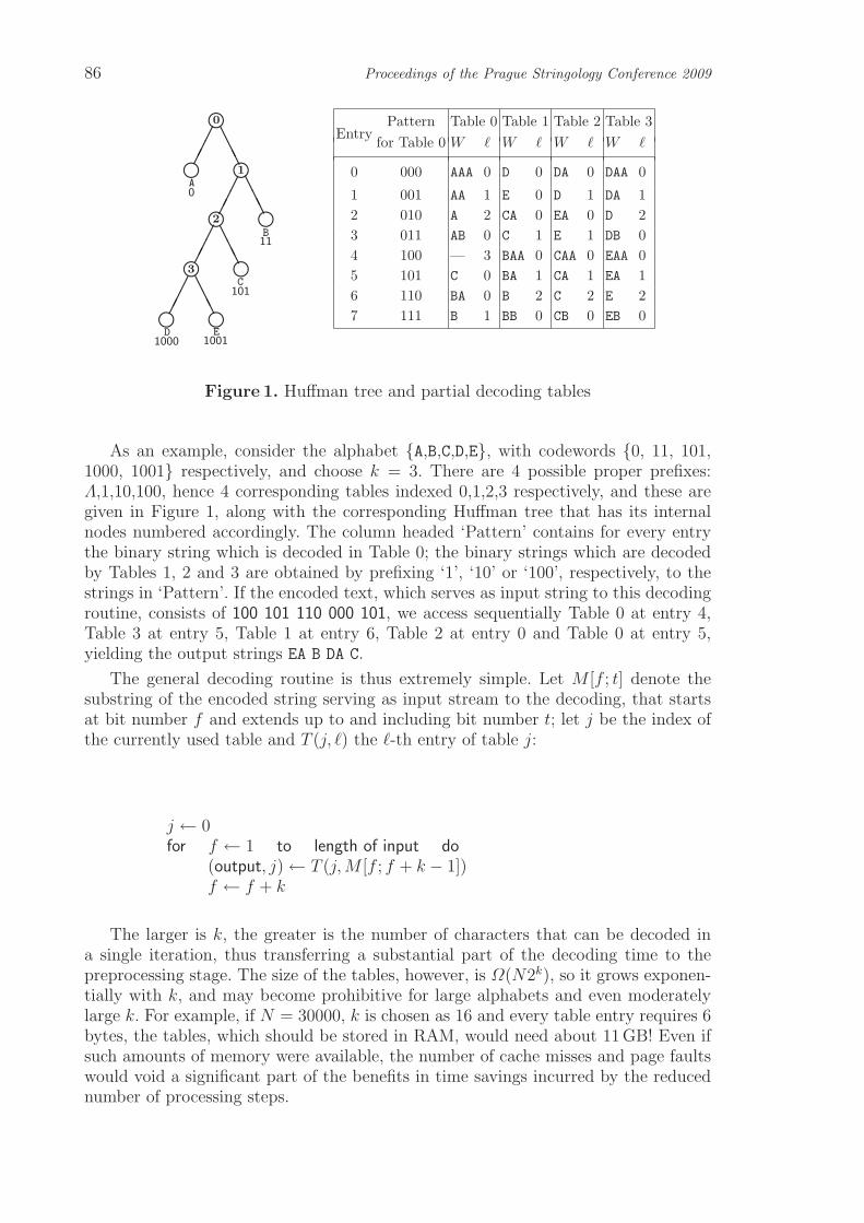
86 Proceedings of the Prague Stringology Conference 2009
3
0
11
101
1000 1001ED
C
A
2
B
0
1
EntryPattern Table 0 Table 1 Table 2 Table 3
for Table 0 W ℓ W ℓ W ℓ W ℓ
0 000 AAA 0 D 0 DA 0 DAA 0
1 001 AA 1 E 0 D 1 DA 1
2 010 A 2 CA 0 EA 0 D 2
3 011 AB 0 C 1 E 1 DB 0
4 100 — 3 BAA 0 CAA 0 EAA 0
5 101 C 0 BA 1 CA 1 EA 1
6 110 BA 0 B 2 C 2 E 2
7 111 B 1 BB 0 CB 0 EB 0
Figure 1. Huffman tree and partial decoding tables
As an example, consider the alphabet A,B,C,D,E, with codewords 0, 11, 101,1000, 1001 respectively, and choose k = 3. There are 4 possible proper prefixes:Λ,1,10,100, hence 4 corresponding tables indexed 0,1,2,3 respectively, and these aregiven in Figure 1, along with the corresponding Huffman tree that has its internalnodes numbered accordingly. The column headed ‘Pattern’ contains for every entrythe binary string which is decoded in Table 0; the binary strings which are decodedby Tables 1, 2 and 3 are obtained by prefixing ‘1’, ‘10’ or ‘100’, respectively, to thestrings in ‘Pattern’. If the encoded text, which serves as input string to this decodingroutine, consists of 100 101 110 000 101, we access sequentially Table 0 at entry 4,Table 3 at entry 5, Table 1 at entry 6, Table 2 at entry 0 and Table 0 at entry 5,yielding the output strings EA B DA C.
The general decoding routine is thus extremely simple. Let M [f ; t] denote thesubstring of the encoded string serving as input stream to the decoding, that startsat bit number f and extends up to and including bit number t; let j be the index ofthe currently used table and T (j, ℓ) the ℓ-th entry of table j:
j ← 0for f ← 1 to length of input do
(output, j)← T (j,M [f ; f + k − 1])f ← f + k
The larger is k, the greater is the number of characters that can be decoded ina single iteration, thus transferring a substantial part of the decoding time to thepreprocessing stage. The size of the tables, however, is Ω(N2k), so it grows exponen-tially with k, and may become prohibitive for large alphabets and even moderatelylarge k. For example, if N = 30000, k is chosen as 16 and every table entry requires 6bytes, the tables, which should be stored in RAM, would need about 11 GB! Even ifsuch amounts of memory were available, the number of cache misses and page faultswould void a significant part of the benefits in time savings incurred by the reducednumber of processing steps.

Shmuel T. Klein and Dana Shapira: On the Usefulness of Backspace 87
4.2 Using backspaces to get another time/space tradeoff
The number of tables, and thus the storage requirements, can be reduced, by con-ceptually modifying the text with the introduction of backspace characters at certainlocations. Particularly in the case of a large alphabet, the blocksize k could be chosensmaller than the longest codeword, and tables would be constructed not for all theinternal nodes, but only for those on levels that are multiples of k, that is for theroot (level 0), and all the internal nodes on levels k, 2k, 3k, etc. There is an obviousgain in the number of tables, which comes at the price of a slower decoding pace: asbefore, the table entries consist first of the decoding W of a bit string B obtainedby concatenating some prefix to the binary representation of the entry index. If Bis not completely decipherable, the remainder Pj is used in the previous setting asindex to the next table. For the new variant, if |Pj|, the length of the remainder, issmaller than k, then no corresponding table has been stored, so these |Pj| bits haveto be reread in the next iteration. This is enforced by adding, after the remainder,|Pj| backspaces into the text.
EntryPattern Table 0 Table 3
for Table 0 W ℓ b W ℓ b
0 000 AAA 0 0 DAA 0 0
1 001 AA 0 1 DA 0 1
2 010 A 0 2 D 0 2
3 011 AB 0 0 DB 0 0
4 100 — 3 0 EAA 0 0
5 101 C 0 0 EA 0 1
6 110 BA 0 0 E 0 2
7 111 B 0 1 EB 0 0
Figure 2. Reduced partial decoding tables
It should however be noted, that the modification of the text is only conceptual,and will manifest itself only in the modified decoding routine; the encoded text itselfneed not to be touched, so there is no loss in compression efficiency, only in decodingspeed. The table entries for the new algorithm are thus extended to include a thirdcomponent: a back skip b, indicating how many backspaces should have been intro-duced at that particular point, which is equivalent to the number of bits the pointerinto the input string should be moved back. Using the above notations, T (j, i) willconsist of the triplet (W, ℓ, b), and the decoding routine is given by
j ← 0 back ← 0for f ← 1 to length of input do
(output, j, back)← T (j,M [f ; f + k − 1])f ← f + k − back
As example, consider the same Huffman tree and the same input string as abovewith k = 3. Only two tables remain, Table 0 and Table 3, given in Figure 2. Decodingis now performed by six table accesses rather than only 5 with the original tables,

88 Proceedings of the Prague Stringology Conference 2009
using the sequence of blocks 100, 101, BS11, BS00, 001, BS01 to access tables 0, 3, 0,0, 3, 0, respectively, where the backspace BS indicates that the preceding bit is readagain, resulting in an overlap of the currently decoded block with the preceding one.
Figure 3 shows the input string and above it its parsing into codewords usingthe standard Huffman decoding. Below appear first the parsing into consecutive k-bit blocks using the original tables, then the parsing into partially overlapping k-bitblocks with the tables relying on the backspaces. Note that for simplicity, we do notdeal here with the case that the last block may be shorter than k bits.
E A B D A C
1 0 0 1 0 1 1 1 0 0 0 0 1 0 1
— EA B DA C
— EA B — DA C
Figure 3. Example using original and reduced tables
To get some experimental results, we used the King James Bible (KJB) as above,and Wall Street Journal (WSJ) issues that appeared in 1989. Huffman codes weregenerated for large “alphabets”, consisting of entire words. Some of the relevantstatistics are given in Table 3, and the results are presented in Table 4. The rowheaded Bit corresponds to the regular bit per bit Huffman decoding. The next rowbrings the values of the Partial decoding Tables of [3] described in Section 4.1 above,and the row with title reduced corresponds to the variant with the backspaces.
For each of the test databases, the first column brings the maximal size k of theblock of bits that is decoded as one unit. The next column, headed bpa is in fact theaverage value of k used during the decoding. It is the average number of decodedbits per table access, evaluated as the size of the compressed file in bits divided bythe total number of such accesses. The next column brings timing results, in terms ofthe number of MB that can be processed per second on our test machine. The timefor the variant with the full tables for WSJ could not be evaluated, due to exceedingRAM requirements. The last column, headed RAM, gives the size of the requiredauxiliary storage in MB. We see that the Reduced Tables saved 50 to 80 % of thespace required by the partial decoding tables, while using the same k, reducing thedecoding rate only by about 20 %.
full compression number of averagesize ratio words word length
KJB 3.1 MB 5.15 MB 11669 8.8 bitWSJ 36.5 MB 5.05 MB 115136 11.2 bit
Table 3. Statistical data on test files

Shmuel T. Klein and Dana Shapira: On the Usefulness of Backspace 89
KJB WSJk bpa MB/sec RAM k bpa MB/sec RAM
Bit 1 1 10.1 0.21 1 1 6,6 2.1Tables 8 8 0.4 17 8 8 — 197reduced 8 6.37 13.7 8.7 8 6.35 7.6 34.1
Table 4. Experimental comparison of decoding
5 Conclusion
We presented three examples of applications in various areas of Information RetrievalSystems, for which the inclusion of a backspace character in the alphabet may leadto improved performance. The main message we hoped to convey in this study, isthat the definition of alphabets in the broadest sense as used in IR systems, does nothave to be restricted to collections of classical items such as letters, words or strings,but may be extended to include also conceptual elements such as a backspace, which,even if not materialized as the other elements, may at times have helpful usages.
References
1. K. C.-C. Chang, H. Garcia-Molina, and A. Paepcke: Predicate rewriting for translatingBoolean queries in a heterogeneous information system. ACM Trans. on Information Systems,17(1) 1999, pp. 1–39.
2. Y. Choueka: Responsa: A full-text retrieval system with linguistic processing for a 65-millionword corpus of jewish heritage in Hebrew. IEEE Data Eng. Bull., 14(4) 1989, pp. 22–31.
3. Y. Choueka, S. T. Klein, and Y. Perl: Efficient variants of Huffman codes in high levellanguages, in Proc. 8-th ACM-SIGIR Conference, Montreal, Canada, 1985, pp. 122–131.
4. A. S. Fraenkel: All about the Responsa Retrieval Project you always wanted to know but wereafraid to ask, Expanded Summary. Jurimetrics J., 16 1976, pp. 149–156.
5. W. B. Frakes: Stemming algorithms, in Information Retrieval, Data Structures and Algo-rithms, W. B. Frakes and R. Baeza-Yates, eds., Prentice Hall, NJ, 1992, pp. 131–160.
6. D. Huffman: A method for the construction of minimum redundancy codes, in Proc. of theIRE, vol. 40, 1952, pp. 1098–1101.
7. S. T. Klein: On the use of negation in Boolean IR queries. Information Processing & Man-agement, 45 2009, pp. 298–311.
8. A. Moffat and Z. J.: Adding compression to a full-text retrieval system. Software — Practice& Experience, 25(8) 1995, pp. 891–903.
9. G. Salton, A. Wong, and C. S. Yang: A vector space model for automatic indexing.Communications of the ACM, 18(11) 1975, pp. 613–620.
10. A. Sieminski: Fast decoding of Huffman codes. Information Processing Letters, 26 1998, pp. 237–241.
11. K. Sparck Jones, S. Walker, and S. E. Robertson: A probabilistic model of informationretrieval: development and comparative experiments – parts 1 and 2. Information Processing& Management, 36(6) 2000, pp. 779–840.
12. C. Tryfonopoulos, M. Koubarakis, and Y. Drougas: Filtering algorithms for infor-mation retrieval models with named attributes and proximity operators, in Proc. SIGIR Conf.,Sheffield, UK, 2004, pp. 313–320.
13. J. Veronis and P. Langlais: Evaluation of parallel text alignment systems: The ARCADEproject, in Parallel Text Processing, J. Veronis, ed., Kluwer Academic Publishers, Dordrecht,2000, pp. 369–388.
14. I. H. Witten, A. Moffat, and T. C. Bell: Managing Gigabytes: Compressing and IndexingDocuments and Images, Van Nostrand Reinhold, New York, 1994.

An Efficient Algorithm for
Approximate Pattern Matching with Swaps
Matteo Campanelli1, Domenico Cantone2, Simone Faro2, and Emanuele Giaquinta2
1 Universita di Catania, Scuola Superiore di CataniaVia San Nullo 5/i, I-95123 Catania, Italy
2 Universita di Catania, Dipartimento di Matematica e InformaticaViale Andrea Doria 6, I-95125 Catania, Italy
[email protected], cantone | faro | [email protected]
Abstract. The Pattern Matching problem with Swaps consists in finding all occur-rences of a pattern P in a text T , when disjoint local swaps in the pattern are allowed.In the Approximate Pattern Matching problem with Swaps one seeks to compute, forevery text location with a swapped match of P , the number of swaps necessary toobtain a match at the location.In this paper, we present new efficient algorithms for the Approximate Swap Matchingproblem. In particular, we first present aO(nm2) algorithm, where m is the length of thepattern and n is the length of the text, which is a variation of the Backward-Cross-
Sampling algorithm, a recent solution to the swap matching problem. Subsequently, wepropose an efficient implementation of our algorithm, based on the bit-parallelism tech-nique. The latter solution achieves a O(mn)-time and O(σ)-space complexity, where σis the dimension of the alphabet.From an extensive comparison with some of the most recent and effective algorithmsfor the approximate swap matching problem, it turns out that our algorithms are veryflexible and achieve very good results in practice.
Keywords: approximate pattern matching with swaps, nonstandard pattern match-ing, combinatorial algorithms on words, design and analysis of algorithms
1 Introduction
The Pattern Matching problem with Swaps (Swap Matching problem, for short) is awell-studied variant of the classic Pattern Matching problem. It consists in finding alloccurrences, up to character swaps, of a pattern P of length m in a text T of lengthn, with P and T sequences of characters drawn from a same finite alphabet Σ of sizeσ. More precisely, the pattern is said to swap-match the text at a given location j ifadjacent pattern characters can be swapped, if necessary, so as to make it identicalto the substring of the text ending (or, equivalently, starting) at location j. All swapsare constrained to be disjoint, i.e., each character can be involved in at most oneswap. Moreover, we make the agreement that identical adjacent characters are notallowed to be swapped.
This problem is of relevance in practical applications such as text and music retrie-val, data mining, network security, and many others. Following [6], we also mention aparticularly important application of the swap matching problem in biological com-puting, specifically in the process of translation in molecular biology, with the genetictriplets (otherwise called codons). In such application one wants to detect the possiblepositions of the start and stop codons of an mRNA in a biological sequence and findhints as to where the flanking regions are relative to the translated mRNA region.
Matteo Campanelli, Domenico Cantone, Simone Faro, Emanuele Giaquinta: An Efficient Algorithm for Approximate Pattern Matching with Swaps,
pp. 90–104.
Proceedings of PSC 2009, Jan Holub and Jan Zd’arek (Eds.), ISBN 978-80-01-04403-2 c© Czech Technical University in Prague, Czech Republic

M. Campanelli, D. Cantone, S. Faro, E. Giaquinta: An Efficient Algorithm for. . . 91
The swap matching problem was introduced in 1995 as one of the open problemsin nonstandard string matching [12]. The first nontrivial result was reported by Amir
et al. [1], who provided a O(nm13 log m)-time algorithm in the case of alphabet sets
of size 2, showing also that the case of alphabets of size exceeding 2 can be reducedto that of size 2 with a O(log2 σ)-time overhead (subsequently reduced to O(log σ) inthe journal version [2]). Amir et al. [4] studied some rather restrictive cases in which aO(m log2 m)-time algorithm can be obtained. More recently, Amir et al. [3] solved theswap matching problem in O(n log m log σ)-time. We observe that the above solutionsare all based on the fast Fourier transform (FFT) technique.
In 2008 the first attempt to provide an efficient solution to the swap matchingproblem without using the FFT technique has been presented by Iliopoulos and Rah-man in [11]. They introduced a new graph-theoretic approach to model the problemand devised an efficient algorithm, based on the bit-parallelism technique [7], whichruns in O((n + m) log m)-time, provided that the pattern size is comparable to theword size in the target machine.
More recently, in 2009, Cantone and Faro [9] presented a first approach for solvingthe swap matching problem with short patterns in linear time. Their algorithm, namedCross-Sampling, though characterized by a O(nm) worst-case time complexity,admits an efficient bit-parallel implementation, named BP-Cross-Sampling, whichachievesO(n) worst-case time andO(σ) space complexity in the case of short patternsfitting in few machine words.
In a subsequent paper [8] a more efficient algorithm, named Backward-Cross-
Sampling and based on a similar structure as the one of the Cross-Sampling al-gorithm, has been proposed. The Backward-Cross-Sampling scans the text fromright to left and has a O(nm2)-time complexity, whereas its bit-parallel implemen-tation, named BP-Backward-Cross-Sampling, works in O(mn)-time and O(σ)-space complexity. However, despite their higher worst-case running times, in practicethe algorithms Backward-Cross-Sampling and BP-Backward-Cross-Samp-
ling show a better behavior than their predecessors Cross-Sampling and BP-
Cross-Sampling, respectively.
In this paper we are interested in the approximate variant of the swap matchingproblem. The Approximate Pattern Matching problem with Swaps seeks to compute,for each text location j, the number of swaps necessary to convert the pattern to thesubstring of length m ending at text location j.
A straightforward solution to the approximate swap matching problem consists insearching for all occurrences (with swap) of the input pattern P , using any algorithmfor the standard swap matching problem. Once a swap match is found, to get thenumber of swaps, it is sufficient to count the number of mismatches between thepattern and its swap occurrence in the text and then divide it by 2.
In [5] Amir et al. presented an algorithm that counts in time O(log m log σ) thenumber of swaps at every location containing a swapped matching, thus solving theapproximate pattern matching problem with swaps in O(n log m log σ)-time.
In [9] Cantone and Faro presented also an extension of the Cross-Sampling algo-rithm, named Approximate-Cross-Sampling, for the approximate swap matchingproblem. However, its bit-parallel implementation has a notably high space overhead,since it requires (m log(⌊m/2⌋+ 1) + m) bits, with m the length of the pattern.
In this paper we present a variant of the Backward-Cross-Sampling algo-rithm for the approximate swap matching problem, which works in O(nm2)-time

92 Proceedings of the Prague Stringology Conference 2009
and requires O(m)-space. Its bit-parallel implementation, in contrast with the BP-
Approximate-Cross-Sampling algorithm, does not add any space overhead andmaintains a worst-case O(mn)-time and O(σ)-space complexity, when the patternsize is comparable to the word size in the target machine, and is very fast in practice.
The rest of the paper is organized as follows. In Section 2 we recall some prelimi-nary definitions. Then in Section 3 we describe the Approximate-Cross-Sampling
algorithm and its bit-parallel variant. In Section 4 we present a variant of theBackward-Cross-Sampling algorithm for the approximate swap matching prob-lem and its straightforward bit-parallel implementation. Then we compare, in Sec-tion 5, our newly proposed algorithms against the most effective algorithms presentin literature and, finally, we briefly draw our conclusions in Section 6.
2 Notions and Basic Definitions
Given a string P of length m ≥ 0, we represent it as a finite array P [0 ..m − 1] andwrite length(P ) = m. In particular, for m = 0 we obtain the empty string ε. Wedenote by P [i] the (i+1)-st character of P , for 0 ≤ i < length(P ), and by P [i .. j] thesubstring of P contained between the (i+1)-st and the (j +1)-st characters of P , for0 ≤ i ≤ j < length(P ). A k-substring of a string S is a substring of S of length k. Forany two strings P and P ′, we say that P ′ is a suffix of P if P ′ = P [i .. length(P )−1], forsome 0 ≤ i < length(P ). Similarly, we say that P ′ is a prefix of P if P ′ = P [0 .. i− 1],for some 0 ≤ i ≤ length(P ). We denote by Pi the nonempty prefix P [0 .. i] of P oflength i + 1, for 0 ≤ i < m, whereas, if i < 0, we agree that Pi is the empty string ε.Moreover, we say that P ′ is a proper prefix (suffix) of P if P ′ is a prefix (suffix) of Pand |P ′| < |P |. Finally, we write P.P ′ to denote the concatenation of P and P ′.
Definition 1. A swap permutation for a string P of length m is a permutation π :0, ...,m− 1 → 0, ...,m− 1 such that:
(a) if π(i) = j then π(j) = i (characters at positions i and j are swapped);(b) for all i, π(i) ∈ i− 1, i, i + 1 (only adjacent characters are swapped);(c) if π(i) 6= i then P [π(i)] 6= P [i] (identical characters can not be swapped).
For a given string P and a swap permutation π for P , we write π(P ) to denotethe swapped version of P , namely π(P ) = P [π(0)] · P [π(1)] · · ·P [π(m− 1)].
Definition 2. Given a text T of length n and a pattern P of length m, P is saidto swap-match (or to have a swapped occurrence) at location j ≥ m − 1 of T ifthere exists a swap permutation π of P such that π(P ) matches T at location j, i.e.,π(P ) = T [j −m + 1 .. j]. In such a case we write P ∝ Tj.
As already observed, if a pattern P of length m has a swap match ending atlocation j of a text T , then the number k of swaps needed to transform P into itsswapped version π(P ) = T [j −m + 1 .. j] is equal to half the number of mismatchesof P at location j. Thus the value of k lies between 0 and ⌊m/2⌋.
Definition 3. Given a text T of length n and a pattern P of length m, P is said toswap-match (or to have a swapped occurrence) at location j of T with k swaps ifthere exists a swap permutation π of P such that π(P ) matches T at location j andk = |i : P [i] 6= P [π(i)]|/2. In such a case we write P ∝
kTj.

M. Campanelli, D. Cantone, S. Faro, E. Giaquinta: An Efficient Algorithm for. . . 93
Definition 4 (Pattern Matching Problem with Swaps). Given a text T oflength n and a pattern P of length m, find all locations j ∈ m− 1, . . . , n− 1 suchthat P swap-matches with T at location j, i.e., P ∝ Tj.
Definition 5 (Approximate Pattern Matching Problem with Swaps). Givena text T of length n and a pattern P of length m, find all pairs (j, k), with j ∈m− 1, . . . , n − 1 and 0 ≤ k ≤ ⌊m/2⌋, such that P has a swapped occurrence in Tat location j with k swaps, i.e., P ∝
kTj.
The following elementary result will be used later.
Lemma 6 ([9]). Let P and R be strings of length m over an alphabet Σ and supposethat there exists a swap permutation π such that π(P ) = R. Then π is unique.
Proof. Suppose, by way of contradiction, that there exist two different swap permuta-tions π and π′ such that π(P ) = π′(P ) = R. Then there must exist an index i such thatπ(i) 6= π′(i). Without loss of generality, let us assume that π(i) < π′(i) and supposethat i be the smallest index such that π(i) 6= π′(i). Since π(i), π′(i) ∈ i− 1, i, i + 1,by Definition 1(b), it is enough to consider the following three cases:
Case 1: π(i) = i− 1 and π′(i) = i.Then, by Definition 1(a), we have π(i − 1) = i, so that P [π(i − 1)] = P [i] =P [π′(i)] = P [π(i)], thus violating Definition 1(c).
Case 2: π(i) = i and π′(i) = i + 1.Since by Definition 1(a) we have π′(i+1) = i, then P [π′(i+1)] = P [i] = P [π(i)] =P [π′(i)], thus again violating Definition 1(c).
Case 3: π(i) = i− 1 and π′(i) = i + 1.By Definition 1(c) we have π(i− 1) = π′(i + 1) = i. Thus π′(i− 1) 6= i = π(i− 1),contradicting the minimality of i. ⊓⊔
Corollary 7. Given a text T of length n and a pattern P of length m, if P ∝ Tj, fora given position j ∈ m−1, . . . , n−1, then there exists a unique swapped occurrenceof P in T ending at position j. ⊓⊔
3 The Approximate-Cross-Sampling Algorithm
The Approximate-Cross-Sampling algorithm [9] computes the swap occurrencesof all prefixes of a pattern P (of length m) in continuously increasing prefixes of atext T (of length n), using a dynamic programming approach. Additionally, for eachoccurrence of P in T , the algorithm computes also the number of swaps necessary toconvert the pattern in its swapped occurrence.
In particular, during its (j +1)-st iteration, for j = 0, 1, . . . , n−1, it is establishedwhether Pi ∝k
Tj, for each i = 0, 1, . . . ,m − 1, by exploiting information gatheredduring previous iterations as follows.
Let us putSj =Def (i, k) | 0 ≤ i ≤ m− 1 and Pi ∝k
Tjλj =Def
(0, 0) if P [0] = T [j]∅ otherwise ,
for 0 ≤ j ≤ n− 1, and
S ′j =Def (i, k) | 0 ≤ i < m− 1 and (Pi−1 ∝k
Tj−1 ∨ i = 0) and P [i] = T [j + 1] ,

94 Proceedings of the Prague Stringology Conference 2009
S0 S1 S2 S3 S4 S5 Sj Sj+1
S′0 S′1 S′2 S′3 S′4 S′5 S′j S′j+1
Figure 1. A graphic representation of the iterative fashion for computing sets Sj andS ′
j for increasing values of j.
for 1 ≤ j < n− 1. Then the following recurrences hold:
Sj+1 = (i, k) | i ≤ m− 1 and ((i− 1, k) ∈ Sj and P [i] = T [j + 1]) or((i− 1, k − 1) ∈ S ′
j and P [i] = T [j]) ∪ λj+1
S ′j+1 = (i, k) | i < m− 1 and (i− 1, k) ∈ Sj and P [i] = T [j + 2] ∪ λj+2.
(1)
where the base cases are given by S0 = λ0 and S ′0 = λ1.
Such relations allow one to compute the sets Sj and S ′j in an iterative fashion,
where Sj+1 is computed in terms of both Sj and S ′j, whereas S ′
j+1 needs only Sj for itscomputation. The resulting dependency graph has a doubly crossed structure, fromwhich the name of the algorithm in Fig. 2(A), Approximate-Cross-Sampling,for the swap matching problem. Plainly, the time complexity of the Approximate-
Cross-Sampling algorithm is O(nm).
In [9], a bit-parallel implementation of the Approximate-Cross-Sampling al-gorithm, called BP-Approximate-Cross-Sampling, has been presented.
The BP-Approximate-Cross-Sampling algorithm1 uses a representation ofthe sets Sj and S ′
j as lists of qm bits, Dj and D′j respectively, where m is the length
of the pattern and q = log(⌊m/2⌋ + 1) + 1. If (i, k) ∈ Sj, where 0 ≤ i < m and0 ≤ k ≤ ⌊m/2⌋, then the rightmost bit of the i-th block of Dj is set to 1 and theleftmost q − 1 bits of the i-th block correspond to the value k (we need exactly qbits to represent a value between 0 and ⌊m/2⌋). The same considerations hold for thesets S ′
j. Notice that if mq ≤ w, each list fits completely in a single computer word,whereas if mq > w one needs ⌈mq/w⌉ computer words to represent each of the setsSj and S ′
j.For each character c of the alphabet Σ, the algorithm maintains a bit mask M [c],
where the rightmost bit of the i-th block is set to 1 if P [i] = c, and a bit mask B[c],whose i-th block have all its bits set to 1 if P [i] = c.
The algorithm also maintains two bit vectors, D and D′, whose configurationsduring the computation are respectively denoted by Dj and D′
j, as the location j
advances over the input text. For convenience, we introduce also the bit vectors D−1
and D′−1, which are both set to 0qm. While scanning the text from left to right, the
algorithm computes for each position j ≥ 0 the bit vector Dj in terms of Dj−1 andD′
j−1, by performing the following bitwise operations (in brackets the corresponding
operations on the set Sj represented by Dj):
1 Here we provide some minor corrections to the code of the BP-Approximate-Cross-Sampling
algorithm presented in [9].

M. Campanelli, D. Cantone, S. Faro, E. Giaquinta: An Efficient Algorithm for. . . 95
(A) Approximate-Cross-Sampling (P, m, T, n)
1. S00 ← S1
0 ← ∅2. if P [0] = T [0] then S0
0 ← (0, 0)3. if P [0] = T [1] then S1
0 ← (0, 0)4. for j ← 1 to n − 1 do5. S0
j ← S1j ← ∅
6. for (i, k) ∈ S0j−1 do
7. if i < m − 1 then8. if P [i + 1] = T [j]9. then S0
j ← S0j ∪ (i + 1, k)
10. if j < n − 1 and P [i + 1] = T [j + 1]11. then S1
j ← S1j ∪ (i + 1, k)
12. else Output((j − 1, k))13. for (i, k) ∈ S1
j−1 do
14. if i < m − 1 and P [i + 1] = T [j − 1]15. then S0
j ← S0j ∪ (i + 1, k + 1)
16. if P [0] = T [j] then S0j ← S0
j ∪ (0, 0)17. if j < n − 1 and P [0] = T [j + 1]18. then S1
j ← S1j ∪ (0, 0)
19. for (i, k) ∈ S0n−1 do
20. if i = m − 1 then Output(n − 1, k)
(B) BP-Approximate-Cross-Sampling (P, m, T, n)
1. q ← log(⌊m/2⌋ + 1) + 12. F ← 0qm−11
3. G ← 0q(m−1)1q
4. for c ∈ Σ do5. M [c] ← 0qm
6. B[c] ← 0qm
7. for i ← 0 to m − 1 do8. M [P [i]] ← M [P [i]] | F9. B[P [i]] ← B[P [i]] | G10. F ← (F ≪ q)11. G ← (G ≪ q)
12. F ← 0q−110q(m−1)
13. D ← D′ ← 0qm
14. for j ← 0 to n − 1 do15. H0 ← (D ≪ q) | 116. H1 ← (D′ ≪ q) & B[T [j − 1]17. H2 ← (D′ ≪ q) & M [T [j − 1]18. D ← (H0 & B[T [j]]) | H1
19. D ← D + (H2 ≪ 1)20. D′ ← (H0 & B[T [j + 1]]) & ∼ D21. if (D & F ) 6= 0qm then22. k ← (D ≫ (q(m − 1) + 1))23. Output(j, k)
Figure 2. (A) The Approximate-Cross-Sampling algorithm for the approxim-ate swap matching problem. (B) Its bit-parallel variant BP-Approximate-Cross-
Sampling.
Dj ← Dj−1 ≪ q [ Sj = (i, k) : (i− 1, k) ∈ Sj−1 ]Dj ← Dj | 1 [ Sj = Sj ∪ (0, 0) ]Dj ← Dj & B[T [j]] [ Sj = Sj \ (i, k) : P [i] 6= T [j] ]Dj ← Dj | H1 [ Sj = Sj ∪K ]Dj ← Dj + (H2 ≪ 1) [∀ (i, k) ∈ K change (i, k) with (i, k + 1) in Sj ]
where H1 = ((D′j−1 ≪ q) & B[T [j − 1]]), H2 = ((D′
j−1 ≪ q) & M [T [j − 1]]), and
K = (i, k) : (i− 1, k) ∈ S ′j−1 ∧ P [i] = T [j − 1].
Similarly, the bit vector D′j is computed in the j-th iteration of the algorithm
in terms of Dj−1, by performing the following bitwise operations (in brackets thecorresponding operations on the set S ′
j represented by D′j):
D′j ← Dj−1 ≪ q [ S ′
j = (i, k) : (i− 1, k) ∈ Sj−1 ]D′
j ← D′j | 1 [ S ′
j = S ′j ∪ (0, 0) ]
D′j ← D′
j & B[T [j + 1]] [ S ′j = S ′
j \ (i, k) : P [i] 6= T [j + 1] ]D′
j ← D′j & ∼ Dj [ S ′
j = S ′j \ (i, k) : (i, k) ∈ Sj ].
During the j-th iteration, if the rightmost bit of the (m− 1)-st block of Dj is setto 1, i.e. if (Dj & 10q(m−1)) 6= 0m, a swap match is reported at position j. The totalnumber of swaps is contained in the q− 1 leftmost bits of the (m− 1)-st block of Dj,which can be retrieved by performing a bitwise shift on Dj of (q(m−1)+1) positionsto the right.
The code of the BP-Approximate-Cross-Sampling algorithm is shown inFig. 2(B). It achieves a O(⌈mn log m/w⌉) worst-case time complexity and requiresO(σ⌈m log m/w⌉) extra space, where σ is the size of the alphabet. If m(log(⌊m/2⌋+1) + 1) ≤ c1w, where c1 is a small integer constant, then the algorithm requiresO(n)-time and O(σ) extra space.
96 Proceedings of the Prague Stringology Conference 2009
4 New Algorithms for the Approximate Swap MatchingProblem
In this section we present a new practical algorithm for solving the swap match-ing problem, called Approximate-BCS (Approximate Backward Cross Sampling),which is characterized by a O(mn2)-time and O(m)-space complexity, where m andn are the length of the pattern and text, respectively.
Our algorithm is an extension of the Backward-Cross-Sampling algorithm [8],for the standard swap matching problem. It inherits from the Approximate-Cross-
Sampling algorithm the same doubly crossed structure in its iterative computation,but searches for all occurrences of the pattern in the text by scanning charactersbackwards, from right to left.
Later, in Section 4.2, we present an efficient implementation based on bit par-allelism of the Approximate-BCS algorithm, which achieves a O(mn)-time andO(σ)-space complexity, when the pattern fits within few computer words, i.e., ifm ≤ c1w, for some small constant c1.
4.1 The Approximate-BCS Algorithm
The Approximate-BCS algorithm searches for all the swap occurrences of a pat-tern P (of length m) in a text T (of length n) using right-to-left scans in windows ofsize m, as in the Backward DAWG Matching (BDM) algorithm for the exact singlepattern matching problem [10]. In addition, for each occurrence of P in T , the algo-rithm counts the number of swaps necessary to convert the pattern in its swappedoccurrence.
The BDM algorithm processes the pattern by constructing a directed acyclic wordgraph (DAWG) of the reversed pattern. The text is processed in windows of size mwhich are searched for the longest prefix of the pattern from right to left by meansof the DAWG. At the end of each search phase, either a longest prefix or a match isfound. If no match is found, the window is shifted to the start position of the longestprefix, otherwise it is shifted to the start position of the second longest prefix.
As in the BDM algorithm, the Approximate-BCS algorithm processes the textin windows of size m. Each attempt is identified by the last position, j, of the currentwindow of the text. The window is searched for the longest prefix of the patternwhich has a swapped occurrence ending at position j of the text. At the end of eachattempt, a new value of j is computed by performing a safe shift to the right of thecurrent window in such a way to left-align it with the longest prefix matched in theprevious attempt.
To this end, if we put
Shj =Def h− 1 ≤ i ≤ m− 1 | P [i− h + 1 .. i] ∝ Tj ,Wh
j =Def h ≤ i < m− 1 | P [i− h + 2 .. i] ∝ Tj and P [i− h + 1] = T [j − h] ,for 0 ≤ j < n and 0 ≤ h ≤ m, then the following recurrences hold:
Sh+1j = h− 1 ≤ i ≤ m− 1 | (i ∈ Sh
j and P [i− h] = T [j − h]) or(i ∈ Wh
j and P [i− h] = T [j − h + 1]) Wh+1
j = h ≤ i ≤ m− 1 | i ∈ Shj and P [i− h] = T [j − h− 1] .
(2)
where the base cases are given by
S0j = i | 0 ≤ i < m and W0
j = 0 ≤ i < m− 1 | P [i + 1] = T [j] .

M. Campanelli, D. Cantone, S. Faro, E. Giaquinta: An Efficient Algorithm for. . . 97
Sℓj
Wℓj
S2j
W2j
S1j
W1j
S0j
W0j
Shu
Whu
S2u
W2u
S1u
W1u
S0u
W0u
u = j + m− ℓ
Figure 3. A graphic representation of the iterative fashion for computing the sets Shj
andWhj for increasing values of h. A first attempt starts at position j of the text and
stops with h = ℓ. The subsequent attempt starts at position u = j + m− l.
Such relations allow one to compute the sets Shj and Wh
j in an iterative fashion,
where Sh+1j is computed in terms of both Sh
j and Whj , whereas Wh+1
j needs only Shj
for its computation. The resulting dependency graph has a doubly crossed structureas shown in Figure 3.
Plainly the set Shj includes all the values i such that the h-substring of P ending at
position i has a swapped occurrence ending at position j in T . Thus, if (h− 1) ∈ Shj ,
then there is a swapped occurrence of the prefix of length h of P . Hence, it followsthat P has a swapped occurrence ending at position j if and only if (m− 1) ∈ Sm
j .Observe however that the only prefix of length m is the pattern P itself. Thus
(m− 1) ∈ Smj if and only if Sm
j 6= ∅.The following result follows immediately from (2).
Lemma 8. Let P and T be a pattern of length m and a text of length n, respectively.Moreover let m − 1 ≤ j ≤ n − 1 and 0 ≤ i < m. If i ∈ Sγ
j , then it follows that
i ∈ (Shj ∪W h
j ), for 1 ≤ h ≤ γ. ⊓⊔Lemma 9. Let P and T be a pattern of length m and a text of length n, respectively.Then, for every m− 1 ≤ j ≤ n− 1 and 0 ≤ i < m such that i ∈ (Sγ
j ∩W γ−1j ∩ Sγ−1
j ),we have P [i− γ + 1] = P [i− γ + 2].
Proof. From i ∈ (Sγj ∩ Sγ−1
j ) it follows that P [i − γ + 1] = T [j − γ + 1]. Also, from
i ∈ W γ−1j it follows that P [i−γ+2] = T [j−γ+1]. Thus P [i−γ+1] = P [i−γ+2]. ⊓⊔
The following lemma will be used.
Lemma 10. Let P and T be a pattern of length m and a text of length n, respectively.Moreover let m − 1 ≤ j ≤ n − 1 and 0 ≤ i < m. Then, if i ∈ Sγ
j , there is a swap
between characters P [i− γ + 1] and P [i− γ + 2] if and only if i ∈ (Sγj \ Sγ−1
j ).
Proof. Before entering into details we remember that, by Definition 1, a swap cantake place between characters P [i−γ +1] and P [i−γ +2] if and only if P [i−γ +1] =T [j − γ + 2], P [i− γ + 2] = T [j − γ + 1] and P [i− γ + 1] 6= P [i− γ + 2].
Now, suppose that i ∈ Sγj and that there is a swap between characters P [i−γ +1]
and P [i− γ + 2]. We proceed by contradiction to prove that i /∈ Sγ−1j . Thus, we have

98 Proceedings of the Prague Stringology Conference 2009
(i) i ∈ Sγj (by hypothesis)
(ii) P [i− γ + 2] = T [j − γ + 1] 6= P [i− γ + 1] (by hypothesis)
(iii) i ∈ Sγ−1j (by contradiction)
(iv) i /∈ W γ−1j (by (ii), (iii), and Lemma 9)
(v) P [i− γ + 1] = T [j − γ + 1] (by (i) and (iv))obtaining a contradiction between (ii) and (v).
Next, suppose that i ∈ (Sγj \ Sγ−1
j ). We prove that there is a swap betweencharacters P [i− γ + 1] and P [i− γ + 2]. We have
(i) i ∈ Sγj and i /∈ Sγ−1
j (by hypothesis)
(ii) i ∈ W γ−1j (by (i) and Lemma 8)
(iii) i ∈ Sγ−2j (by (ii) and (2))
(iv) P [i− γ + 1] = T [j − γ + 2] (by (i) and (ii))(v) P [i− γ + 2] = T [j − γ + 1] (by (ii))(vi) P [i− γ + 2] 6= T [j − γ + 2] = P [i− γ + 1] (by (i) and (iii)).
⊓⊔
The following corollary is an immediate consequence of Lemmas 10 and 8.
Corollary 11. Let P and T be strings of length m and n, respectively, over a commonalphabet Σ. Then, for m−1 ≤ j ≤ n−1, P has a swapped occurrence in T at locationj with k swaps, i.e., P ∝
kTj, if and only if
(m− 1) ∈ Smj and |∆j| = k ,
where ∆j = 1 ≤ h < m : (m− 1) ∈ (Sh+1j \ Sh
j ). ⊓⊔
In consideration of the preceding corollary, the Approximate-BCS algorithmmaintains a counter which is incremented every time (m− 1) ∈ (Sh+1
j \ Shj ), for any
1 < h ≤ m, in order to count the swaps for an occurrence ending at a given positionj of the text.
For any attempt at position j of the text, let us denote by ℓ the length of thelongest prefix matched in the current attempt. Then the algorithm starts its compu-tation with j = m − 1 and ℓ = 0. During each attempt, the window of the text isscanned from right to left, for h = 1, . . . ,m. If, for a given value of h, the algorithmdiscovers that (h− 1) ∈ Sh
j , then ℓ is set to the value h.The algorithm is not able to remember the characters read in previous iterations.
Thus, an attempt ends successfully when h reaches the value m (a match is found),or unsuccessfully when both sets Sh
j and Whj are empty. In any case, at the end of
each attempt, the start position of the window, i.e., position j −m + 1 in the text,can be shifted to the start position of the longest proper prefix detected during thebackward scan. Thus the window is advanced m − ℓ positions to the right. Observethat since ℓ < m, we plainly have that m− ℓ > 0.
Moreover, in order to avoid accessing the text character at position j−h+1 = n,when j = n − 1 and h = 0, the algorithm benefits of the introduction of a sentinelcharacter at the end of the text.
The code of the Approximate-BCS algorithm is shown in Figure 4(A). Its timecomplexity is O(nm2) in the worst case and requires O(m) extra space to representthe sets Sh
j and Whj .

M. Campanelli, D. Cantone, S. Faro, E. Giaquinta: An Efficient Algorithm for. . . 99
4.2 The Approximate-BPBCS Algorithm
In [8], an efficient bit-parallel implementation of the Backward-Cross-Sampling
algorithm, called BP-Backward-Cross-Sampling, has also been presented. In thissection we illustrate a practical bit-parallel implementation of the Approximate-
BCS algorithm, named Approximate-BPBCS, along the same lines of the BP-
Backward-Cross-Sampling algorithm.In the Approximate-BPBCS algorithm, the sets Sh
j andWhj are represented as
lists of m bits, Dhj and Ch
j respectively, where m is the length of the pattern.
The (i−h+1)-th bit of Dhj is set to 1 if i ∈ Sj, i.e., if P [i−h+1 .. i] ∝ Tj, whereas
the (i − h + 1)-th bit of Chj is set to 1 if i ∈ Wh
j , i.e., if P [i − h + 2 .. i] ∝ Tj andP [i − h + 1] = T [j − h]. All remaining bits are set to 0. Notice that if m ≤ w, eachbit vector fits in a single computer word, whereas if m > w we need ⌈m/w⌉ computerwords to represent each of the sets Sh
j and Whj .
For each character c of the alphabet Σ, the algorithm maintains a bit mask M [c]whose i-th bit is set to 1 if P [i] = c.
As in the Approximate-BCS algorithm, the text is processed in windows of sizem, identified by their last position j, and the first attempt starts at position j = m−1.For any searching attempt at location j of the text, the bit vectors D1
j and C1j are
initialized to M [T [j]] | (M [T [j + 1]]&(M [T [j]] ≪ 1)) and M [T [j − 1]], respectively,according to the recurrences (2) and relative base cases. Then the current windowof the text, i.e., T [j −m + 1 .. j], is scanned from right to left, by reading characterT [j − h + 1], for increasing values of h. Namely, for each value of h > 1, the bitvector Dh+1
j is computed in terms of Dhj and Ch
j , by performing the following bitwiseoperations:
(a) Dh+1j ← (Dh
j ≪ 1) & M [T [j − h]]
(b) Dh+1j ← Dh+1
j | ((Chj ≪ 1) & M [T [j − h + 1]]) .
Concerning (a), by a left shift of Dhj , all elements of Sh
j are added to the set Sh+1j .
Then, by performing a bitwise and with the mask M [T [j − h]], all elements i suchthat P [i− h] 6= T [j − h] are removed from Sh+1
j . Similarly, the bit operations in (b)
have the effect to add to Sh+1j all elements i in Wh
j such that P [i− h] = T [j− h + 1].Formally, we have:
(a′) Sh+1j ← Sh
j \ i ∈ Shj : P [i− h] 6= T [j − h]
(b′) Sh+1j ← Sh+1
j ∪Whj \ i ∈ Wh
j : P [i− h] 6= T [j − h + 1] .
Similarly, the bit vector Ch+1j is computed in terms of Dh
j , by performing thefollowing bitwise operations
(c) Ch+1j ← (Dh
j ≪ 1) & M [T [j − h− 1]]
which have the effect to add to the set Wh+1j all elements of the set Sh
j (by shifting
Dhj to the left by one position) and to remove all elements i such P [i] 6= T [j − h− 1]
holds (by a bitwise and with the mask M [T [j − h− 1]]), or, more formally:
(c′) Wh+1j ← Sh
j \ i ∈ Shj : P [i− h] 6= T [j − h− 1] .
In order to count the number of swaps, observe that the (i− h + 1)-th bit of Dhj
is set to 1 if i ∈ Shj . Thus, the condition (m − 1) ∈ (Sh+1
j \ Shj ) can be implemented
by the following bitwise condition:
(d) ((Dh+1 & ∼ (Dh ≪ 1)) & (1≪ h)) 6= 0 .

100 Proceedings of the Prague Stringology Conference 2009
(A) Approximate-BCS (P, m, T, n)
1. T [n] ← P [0]2. j ← m − 13. while j < n do4. h ← 05. S0
j ← i | 0 ≤ i < m6. W0
j ← 0 ≤ i < m − 1 | P [i + 1] = T [j]7. c ← 08. while h < m and Sh
j ∪Whj 6= ∅ do
9. if (h − 1) ∈ Shj then ℓ ← h
10. for each i ∈ Shj do
11. if i ≥ h and P [i − h] = T [j − h]
12. then Sh+1j ← Sh+1
j ∪ i13. if i > h and P [i − h] = T [j − h − 1]
14. then Wh+1j ← Wh+1
j ∪ i15. for each i ∈ Wh
j do
16. if i ≥ h and P [i − h] = T [j − h + 1]
17. then Sh+1j ← Sh+1
j ∪ i18. if m − 1 ∈ Sh+1
j and m − 1 /∈ Shj
19. then c ← c + 120. h ← h + 121. if (h − 1) ∈ Sh
j then Output(j,c)
22. j ← j + m − ℓ
(B) Approximate-BPBCS (P, m, T, n)
1. F ← 10m−1
2. for c ∈ Σ do M [c] ← 0m
3. for i ← 0 to m − 1 do4. M [P [i]] ← M [P [i]] | F5. F ← F ≫ 16. T [n] ← P [0]7. j ← m − 18. F ← 10m−1
9. while j < n do10. h ← 1, ℓ ← 011. D ← M [T [j]]12. D ← D | (M [T [j + 1]]&(M [T [j]] ≪ 1))13. C ← M [T [j − 1]]14. c ← 015. while h < m and (D | C) 6= 0 do
16. D′ ← D ≪ 1
17. if F&D 6= 0 then ℓ ← h18. H ← (C ≪ 1) & M [T [j − h + 1]]
19. C ← D′
& M [T [j − h − 1]]
20. D ← D′
& M [T [j − h]]21. D ← D | H
22. if (D & ∼ D′
) & (1 ≪ h) 6= 023. then c ← c + 124. h ← h + 125. if D 6= 0 then Output(j,c)26. j ← j + m − ℓ
Figure 4. (A) The Approximate-BCS algorithm for the approximate swap match-ing problem. (B) Its bit-parallel variant Approximate-BPBCS.
As in the Approximate-BCS algorithm, an attempt ends when h = m or(Dh
j |Chj ) = 0. If h = m and Dh
j 6= 0, a swap match at position j of the text is
reported. In any case, if h < m is the largest value such that Dhj 6= 0, then a prefix
of the pattern, of length ℓ = h, which has a swapped occurrence ending at position jof the text, has been found. Thus, a safe shift of m− ℓ position to the right can takeplace.
In practice, two vectors only are enough to implement the sets Dhj and Ch
j , for
h = 0, 1, . . . ,m, as one can transform the vector Dhj into the vector Dh+1
j and the
vector Chj into the vector Ch+1
j , during the h-th iteration of the algorithm at a givenlocation j of the text.
The counter for taking note of the number of swaps requires log(⌊m/2⌋+ 1) bitsto be implemented. This compares favorably with the BP-Approximate-Cross-
Sampling algorithm which uses instead m counters of log(⌊m/2⌋ + 1) bits, one foreach prefix of the pattern.
The resulting Approximate-BPBCS algorithm is shown in Fig. 4(B). It achievesa O(⌈nm2/w⌉) worst-case time complexity and requires O(σ⌈m/w⌉+log(⌊m/2⌋+1))extra space, where σ is the alphabet size. If the pattern fits in few machine words, thenthe algorithm finds all swapped matches and their corresponding counts in O(nm)time and O(σ) extra space.

M. Campanelli, D. Cantone, S. Faro, E. Giaquinta: An Efficient Algorithm for. . . 101
5 Experimental Results
Next we report and comment experimental results relative to an extensive comparisonunder various conditions of the following approximate swap matching algorithms:
– Approximate-Cross-Sampling (ACS)
– BP-Approximate-Cross-Sampling (BPACS)
– Approximate-BCS (ABCS)
– Approximate-BPBCS (BPABCS)
– Iliopoulos-Rahman algorithm with a naive check of the swaps (IR&C)
– BP-Backward-Cross-Sampling algorithm with a naive check of the swaps(BPBCS&C)
We have chosen to include in our comparison also the algorithms IR&C and BP-BCS&C, since the algorithms IR and BPBCS turned out, in [8], to be the most efficientsolutions for the swap matching problem. Instead, the Naive algorithm and algorithmsbased on the FFT technique have not been taken into consideration, as their overheadis quite high, resulting in poor performances.
All algorithms have been implemented in the C programming language and wereused to search for the same strings in large fixed text buffers on a PC with AMDTurion 64 X2 processor with mobile technology TL-60 of 2 GHz and a RAM memoryof 4 GB. In particular, all algorithms have been tested on six Randσ problems, forσ = 4, 8, 16, 32, 64 and 128, on a genome, on a protein sequence, and on a naturallanguage text buffer, with patterns of length m = 4, 8, 12, 16, 20, 24, 28, 32.
In the following tables, running times are expressed in hundredths of seconds andthe best results have been bold-faced.
Running Times for Random ProblemsIn the case of random texts, all algorithms have been tested on six Randσ problems.Each Randσ problem consists in searching a set of 100 random patterns for any givenlength value in a 4 Mb random text over a common alphabet of size σ, with a uniformcharacter distribution.
Running times for a Rand4 problem
m 4 8 12 16 20 24 28 32
ACS 5.916 5.768 5.835 5.860 5.753 5.739 5.571 5.604ABCS 17.132 10.681 8.504 7.278 6.322 6.096 5.778 5.341BPACS 0.817 0.794 0.752 0.800 0.784 0.799 0.818 0.747BPABCS 0.573 0.341 0.255 0.204 0.177 0.159 0.141 0.129IR&C 0.275 0.275 0.275 0.276 0.275 0.279 0.276 0.282BPBCS&C 0.614 0.358 0.262 0.212 0.182 0.161 0.145 0.132
Running times for a Rand8 problem
m 4 8 12 16 20 24 28 32
ACS 4.769 4.756 4.762 4.786 4.761 4.808 4.765 4.796ABCS 11.675 7.273 5.632 4.736 4.167 3.782 3.511 3.305BPACS 0.832 0.830 0.828 0.831 0.830 0.829 0.827 0.827BPABCS 0.413 0.229 0.175 0.145 0.127 0.114 0.104 0.096IR&C 0.282 0.279 0.279 0.277 0.280 0.279 0.283 0.285BPBCS&C 0.388 0.249 0.193 0.157 0.141 0.121 0.111 0.101

102 Proceedings of the Prague Stringology Conference 2009
Running times for a Rand16 problem
m 4 8 12 16 20 24 28 32
ACS 5.210 5.291 5.162 5.282 5.198 5.201 5.202 5.131ABCS 10.200 6.314 5.297 4.554 3.932 3.511 3.448 3.140BPACS 0.786 0.807 0.780 0.783 0.812 0.806 0.743 0.721BPABCS 0.346 0.198 0.144 0.118 0.103 0.093 0.086 0.081IR&C 0.275 0.274 0.279 0.274 0.275 0.277 0.279 0.274BPBCS&C 0.330 0.211 0.155 0.126 0.110 0.099 0.091 0.085
Running times for a Rand32 problem
m 4 8 12 16 20 24 28 32
ACS 5.285 5.080 5.228 5.262 5.175 5.190 5.216 5.296ABCS 9.414 5.831 4.437 3.955 3.521 3.232 2.954 2.890BPACS 0.776 0.746 0.796 0.775 0.834 0.807 0.791 0.796BPABCS 0.294 0.184 0.138 0.113 0.097 0.086 0.078 0.073IR&C 0.275 0.276 0.276 0.276 0.279 0.275 0.275 0.277BPBCS&C 0.285 0.191 0.146 0.119 0.103 0.091 0.083 0.077
Running times for a Rand64 problem
m 4 8 12 16 20 24 28 32
ACS 5.101 5.108 5.254 5.174 5.155 5.098 5.095 5.262ABCS 8.857 5.350 4.165 3.502 3.273 2.972 2.717 2.692BPACS 0.838 0.808 0.769 0.714 0.835 0.806 0.807 0.766BPABCS 0.267 0.162 0.127 0.108 0.095 0.086 0.078 0.073IR&C 0.272 0.276 0.275 0.280 0.281 0.283 0.279 0.279BPBCS&C 0.255 0.165 0.130 0.111 0.098 0.089 0.082 0.076
Running times for a Rand128 problem
m 4 8 12 16 20 24 28 32
ACS 5.070 5.052 5.091 4.996 5.088 4.940 4.968 5.216ABCS 8.672 5.288 3.994 3.289 2.941 2.778 2.660 2.523BPACS 0.833 0.836 0.836 0.836 0.835 0.835 0.836 0.833BPABCS 0.248 0.148 0.115 0.098 0.087 0.080 0.075 0.071IR&C 0.352 0.354 0.354 0.353 0.353 0.353 0.354 0.333BPBCS&C 0.230 0.151 0.117 0.099 0.090 0.082 0.077 0.072
The experimental results show that the BPABCS algorithm obtains the best run-time performance in most cases. In particular, for very short patterns and smallalphabets, our algorithm is second only to the IR&C algorithm. In the case of veryshort patterns and large alphabets, our algorithm is second only to the BPBCS&Calgorithm. In addition we notice that the algorithms IR&C, ACS, and BPACS showa linear behavior, whereas the algorithms ABCS and BPABCS are characterized by adecreasing trend.
Running Times for Real World ProblemsThe tests on real world problems have been performed on a genome sequence andon a natural language text buffer. The genome we used for the tests is a sequenceof 4, 638, 690 base pairs of Escherichia coli taken from the file E.coli of the LargeCanterbury Corpus.1 The tests on the protein sequence have been performed using a2.4 Mb file containing a protein sequence from the human genome with 22 differentcharacters. The experiments on the natural language text buffer have been done withthe file world192.txt (The CIA World Fact Book) of the Large Canterbury Corpus. Thefile contains 2, 473, 400 characters drawn from an alphabet of 93 different characters.
1 http://www.data-compression.info/Corpora/CanterburyCorpus/

M. Campanelli, D. Cantone, S. Faro, E. Giaquinta: An Efficient Algorithm for. . . 103
Running times for a genome segence (σ = 4)
m 4 8 12 16 20 24 28 32
ACS 5.629 5.643 5.654 5.636 5.644 5.640 5.647 6.043ABCS 18.018 11.261 8.805 7.523 6.700 6.117 5.710 5.359BPACS 0.950 0.914 0.917 0.766 0.874 0.934 0.935 0.843BPABCS 0.647 0.318 0.266 0.232 0.195 0.174 0.160 0.147IR&C 0.262 0.287 0.314 0.311 0.311 0.311 0.310 0.311BPBCS&C 0.678 0.367 0.290 0.233 0.204 0.176 0.160 0.146
Running times for a protein sequence (σ = 22)
m 4 8 12 16 20 24 28 32
ACS 3.777 3.784 3.671 3.729 3.766 3.703 3.716 3.741ABCS 7.045 4.557 3.734 3.162 2.806 2.661 2.600 2.351BPACS 0.565 0.581 0.561 0.563 0.584 0.580 0.534 0.519BPABCS 0.249 0.142 0.103 0.084 0.074 0.066 0.061 0.058IR&C 0.388 0.390 0.391 0.389 0.391 0.391 0.396 0.389BPBCS&C 0.241 0.145 0.107 0.087 0.075 0.068 0.062 0.058
Running times for a natural language text buffer (σ = 93)
m 4 8 12 16 20 24 28 32
ACS 3.170 2.757 2.748 2.756 2.761 2.745 2.746 2.754ABCS 6.175 4.054 3.164 2.705 2.306 2.288 2.042 1.866BPACS 0.492 0.497 0.492 0.491 0.492 0.491 0.494 0.493BPABCS 0.194 0.114 0.086 0.071 0.062 0.056 0.051 0.049IR&C 0.171 0.165 0.164 0.168 0.165 0.165 0.165 0.167BPBCS&C 0.164 0.126 0.094 0.076 0.070 0.059 0.056 0.055
From the above experimental results, it turns out that the BPABCS algorithmobtains in most cases the best results and, in the case of very short patterns, is secondto IR&C (for the genome sequence) and to BPBCS&C (for the protein sequence andthe natual language text buffer).
6 Conclusions
In this paper we have presented new efficient algorithms for the Approximate SwapMatching problem. In particular, we have devised an extension of the Backward-
Cross-Sampling general algorithm, named Approximate-BCS, and of its bit-parallel implementation BP-Backward-Cross-Sampling, named Approximate-
BPBCS.
The Approximate-BCS algorithm achieves a O(nm2)-time complexity and re-quiresO(nm) additional space, whereas the Approximate-BPBCS algorithm achie-ves a O(⌈nm2/w⌉) worst-case time complexity and, when the pattern fits in fewmachine words, finds all swapped matches and their corresponding counts in O(nm)-time.
In contrast with the BP-Approximate-Cross-Sampling algorithm, the Ap-
proximate-BPBCS algorithm requires O(σ⌈m/w⌉ + log(⌊m/2⌋ + 1)) extra spaceand is thus preferable to the former in the case of longer patterns.
From an extensive experimentation, it turns out that the Approximate-BPBCS
algorithm is very fast in practice and obtains the best results in most cases, beingsecond only to algorithms based on a naive check of the number of swaps in the caseof very short patterns.

104 Proceedings of the Prague Stringology Conference 2009
References
1. A. Amir, Y. Aumann, G. M. Landau, M. Lewenstein, and N. Lewenstein: Patternmatching with swaps, in IEEE Symposium on Foundations of Computer Science, 1997, pp. 144–153.
2. A. Amir, Y. Aumann, G. M. Landau, M. Lewenstein, and N. Lewenstein: Patternmatching with swaps. Journal of Algorithms, 37(2) 2000, pp. 247–266.
3. A. Amir, R. Cole, R. Hariharan, M. Lewenstein, and E. Porat: Overlap matching.Inf. Comput., 181(1) 2003, pp. 57–74.
4. A. Amir, G. M. Landau, M. Lewenstein, and N. Lewenstein: Efficient special cases ofpattern matching with swaps. Information Processing Letters, 68(3) 1998, pp. 125–132.
5. A. Amir, M. Lewenstein, and E. Porat: Approximate swapped matching. Inf. Process.Lett., 83(1) 2002, pp. 33–39.
6. P. Antoniou, C. Iliopoulos, I. Jayasekera, and M. Rahman: Implementation of a swapmatching algorithm using a graph theoretic model, in Bioinformatics Research and Development,Second International Conference, BIRD 2008, vol. 13 of Communications in Computer andInformation Science, Springer, 2008, pp. 446–455.
7. R. Baeza-Yates and G. H. Gonnet: A new approach to text searching. Commun. ACM,35(10) 1992, pp. 74–82.
8. M. Campanelli, D. Cantone, and S. Faro: A new algorithm for efficient pattern match-ing with swaps, in IWOCA 2009: 20th International Workshop on Combinatorial Algorithms,Lecture Notes in Computer Science, Springer, 2009.
9. D. Cantone and S. Faro: Pattern matching with swaps for short patterns in linear time, inSOFSEM 2009: Theory and Practice of Computer Science, 35th Conference on Current Trendsin Theory and Practice of Computer Science, vol. 5404 of Lecture Notes in Computer Science,Springer, 2009, pp. 255–266.
10. M. Crochemore and W. Rytter: Text algorithms, Oxford University Press, 1994.11. C. S. Iliopoulos and M. S. Rahman: A new model to solve the swap matching problem and
efficient algorithms for short patterns, in SOFSEM 2008, vol. 4910 of Lecture Notes in ComputerScience, Springer, 2008, pp. 316–327.
12. S. Muthukrishnan: New results and open problems related to non-standard stringology, inCombinatorial Pattern Matching, 6th Annual Symposium, CPM 95, vol. 937 of Lecture Notesin Computer Science, Springer, 1995, pp. 298–317.

Searching for Jumbled Patterns in Strings
Ferdinando Cicalese1, Gabriele Fici1, and Zsuzsanna Liptak2
1 Dipartimento di Informatica ed Applicazioni, University of Salerno, Italycicalese,[email protected]
2 AG Genominformatik, Technische Fakultat, Bielefeld University, [email protected]
Abstract. The Parikh vector of a string s over a finite ordered alphabet Σ =a1, . . . , aσ is defined as the vector of multiplicities of the characters, i.e. p(s) =(p1, . . . , pσ), where pi = |j | sj = ai|. Parikh vector q occurs in s if s has a substringt with p(t) = q. The problem of searching for a query q in a text s of length n can besolved simply and optimally with a sliding window approach in O(n) time. We presenttwo new algorithms for the case where the text is fixed and many queries arrive overtime. The first algorithm finds all occurrences of a given Parikh vector in a text (over afixed alphabet of size σ ≥ 2) and appears to have a sub-linear expected time complexity.The second algorithm only decides whether a given Parikh vector appears in a binarytext; it iteratively constructs a linear size data structure which then allows answeringqueries in constant time, for many queries even during the construction phase.
Keywords: Parikh vectors, permuted strings, pattern matching, string algorithms,average case analysis
1 Introduction
Parikh vectors of strings count the multiplicity of the characters. They have beenreintroduced many times by many different names (compomer [5], composition [3],Parikh vector [14], permuted string [7], permuted pattern [9], and others). They arevery natural objects to study, if for nothing else because of the many different appli-cations they appear in; for instance, in computational biology, they have been appliedfor alignment [3], SNP discovery [5], repeated pattern discovery [9], and, most nat-urally, in interpretation of mass spectrometry data [4]. Parikh vectors can be seenas a generalization of strings, where we view two strings as equivalent if one can beturned into the other by permuting its characters; in other words, if the two stringshave the same Parikh vector.
The problem we are interested in here is answering the question whether a queryParikh vector q appears in a given text s (decision version), or where it occurs (oc-currence version). An occurrence of q is defined as an occurrence of a substring tof s with Parikh vector q. The problem can be viewed as an approximate patternmatching problem: We are looking for an occurrence of a jumbled version of a querystring t, i.e. for the occurrence of a substring t′ which has the same Parikh vector. Inthe following, let n be the length of the text s, m the length of the query q (definedas the length of a string t with Parikh vector q), and σ the size of the alphabet.
The above problem (both decision and occurrence versions) can be solved witha simple sliding window based algorithm, in O(n) time and O(σ) additional storagespace. This is worst case optimal with respect to the case of one query. However, whenwe expect to search for many queries in the same string, the above approach leadsto O(Kn) runtime for K queries. To the best of our knowledge, no faster approachis known. This is in stark contrast to the classical exact pattern matching problem:
Ferdinando Cicalese, Gabriele Fici, Zsuzsanna Liptak: Searching for Jumbled Patterns in Strings, pp. 105–117.
Proceedings of PSC 2009, Jan Holub and Jan Zd’arek (Eds.), ISBN 978-80-01-04403-2 c© Czech Technical University in Prague, Czech Republic

106 Proceedings of the Prague Stringology Conference 2009
There, for one query, any naive approach leads to O(nm) runtime, while quite involvedideas for preprocessing and searching are necessary to achieve an improved runtime ofO(n+m), as do the Knuth-Morris-Pratt [12], Boyer-Moore [6] and Boyer-Moore-typealgorithms (see, e.g., [2,10]). However, when many queries are expected, the text canbe preprocessed to produce a data structure of size linear in n, such as a suffix tree,suffix array, or suffix automaton, which then allows to answer individual queries intime linear in the length of the pattern.
In this paper, we present two new algorithms which perform significantly betterthan the naive window algorithm, in the case where many queries arrive. In the courseof both algorithms, a data structure of size O(n) is constructed, which is subsequentlyused for fast searching.
1. For general alphabets: We present the Jumping algorithm (Sect. 3) which usesO(n) space to answer occurrence queries in time O
(σJ log2
(nJ
+ m))
, where Jdenotes the number of iterations of the main loop of the algorithm. We argue thatthe expected value of J for the case of random strings and patterns is O(n/
√σm),
yielding an expected runtime of O(√
σ log2 m√m
n). Our simulations on random strings
and real biological strings indicate that this is indeed the performance of thealgorithm in practice. This is a significant improvement over the naive algorithmw.r.t. expected runtime, both for a single query and repeated queries over onestring.
2. For binary alphabets: After a data structure of size O(n) has been constructed,we answer decision queries in O(1) time (Interval Algorithm, Sect. 4).
The Jumping algorithm is reminiscent of the Boyer-Moore-like approaches to theclassical string matching problem [6,2,10]. This analogy is used both in its presen-tation and in the analysis of the number of iterations performed by the algorithm.We approximate the behavior of the algorithm with a probabilistic automaton, asit is done in [15] to estimate the expected running time of Boyer-Moore on randomstrings.
A straightforward implementation of the Interval Algorithm requires Θ(n2) timefor the preprocessing. Instead we present it employing lazy computation of the datastructure, and thus the runtime is improved such that a query can be answeredeither in O(1) or Θ(n) time, depending on whether the respective entries in the datastructure have already been computed. For K = ω(n) queries, we require Θ(K + n2)time (with either implementation), thus always outperforming the naive algorithm,which has Θ(Kn) runtime. We conjecture that there is no algorithm that can answerany Ω(n) queries in o(n2) time.
Related work: An efficient algorithm for computing all Parikh fingerprints of sub-strings of a given string was developed in [1]. Parikh fingerprints are Boolean vectorswhere the k’th entry is 1 if and only if ak appears in the string. The algorithm in-volves storing a data point for each Parikh fingerprint, of which there are at mostO(nσ) many. This approach was adapted in [9] for Parikh vectors and applied toidentifying all repeated Parikh vectors within a given length range; using it to searchfor queries of arbitrary length would imply using Ω(P (s)) space, where P (s) denotesthe number of different Parikh vectors of substrings of s. This is not desirable, sincethere are strings with quadratic P (s) [8].

F. Cicalese, G. Fici, Zs. Liptak: Searching for Jumbled Patterns in Strings 107
The authors of [7] present an algorithm for finding all occurrences of a Parikhvector in a runlength encoded text. The algorithm’s time complexity is O(n′ + σ),where n′ is the length of the runlength encoding of s. Obviously, if the string is notrunlength encoded, a preprocessing phase of time O(n) has to be added. However,this may still be feasible if many queries are expected. To the best of our knowledge,this is the only algorithm that has been presented for the problem we are treatinghere.
2 Notation and Problem Statement
Let Σ = a1, . . . , aσ be a finite ordered alphabet. For a string s ∈ Σ∗, s = s1 · · · sn,we define the Parikh vector p(s) = (p1, . . . , pσ) by pi := |j | sj = ai|, for i =1, . . . , σ. A Parikh vector p occurs in string s if there are positions i ≤ j such thatp(si · · · sj) = p. We refer to the pair (i, j) as an occurrence of p in s. By convention,we say that the empty string ǫ occurs in each string once. For a Parikh vector p ∈ N
σ,where N denotes the set of non-negative integers, let |p| := ∑
i pi denote the lengthof p, namely the length of any string t with p(t) = p. Further, by s[i, j] = si · · · sj wedenote the substring of s from i to j, for 1 ≤ i ≤ j ≤ n.
For two Parikh vectors p, q ∈ Nσ, we define p ≤ q and p + q component-wise:
p ≤ q if and only if pi ≤ qi for all i = 1, . . . , σ, and p + q = u where ui = pi + qi fori = 1, . . . , σ. Similarly, for p ≤ q, we set q − p = v where vi = qi − pi for i = 1, . . . , σ.
We want to solve the following problem:
Problem Statement: Let s ∈ Σ∗ be given. For a Parikh vector q ∈ Nσ,
1. Decide whether q occurs in s (decision problem);2. Find all occurrences of q in s (occurrence problem).
In the following, let |s| = n and |q| = m. Assume that K many queries arriveover time.
For K = 1, both the decision version and the occurrence version can be solvedoptimally with the following simple algorithm: Move a sliding window of size |q| alongstring s. This way, we encounter all substrings, and thus all Parikh vectors, of length|q|. We maintain the Parikh vector c of the current substring and a counter r whichequals the number of indices i such that ci 6= qi. Each sliding step now costs either0 or 2 update operations of c, depending on whether the new character entering thewindow is the same or different from the one that falls out. Whenever we changethe value of an entry ci, we check whether ci = qi and increment or decrement raccordingly.
This algorithm solves both the decision and occurrence problems and has runningtime Θ(n), using additional storage space Θ(σ). In other words, for one query, it isoptimal (save maybe for the additional storage of Θ(σ)).
Obviously, one can precompute all sub-Parikh vectors of s, store them (sorted,e.g. lexicographically) and do binary search when a query arrives. Preprocessing timeis Θ(n2 log n), because the number of Parikh vectors of s is at most
(n2
)= O(n2),
and there are nontrivial strings with quadratic number of Parikh vectors over arbi-trary alphabets [8]. (Now and in the following, we denote the binary logarithm bylog, the natural logarithm by ln, and otherwise explicitly state the base.) Moreover,simulations reported there have shown that protein strings have quadratically many

108 Proceedings of the Prague Stringology Conference 2009
sub-Parikh vectors, a result relevant for mass spectrometry applications. Query timeis O(log n) for the decision problem and O(log n+M) for the occurrence problem fora query with M occurrences. However, the storage space of Θ(n2) is inacceptable inmany applications.
For small queries, the problem can be solved exhaustively with a linear size index-ing structure such as a suffix tree (size O(n)). We can search up to length m = |q| (ofthe substrings); whenever we find a match, we traverse the subtree below and reportthe leaf numbers, yielding the occurrences of that substring. Total running time isO(σm) for searching the tree down to level m, and O(M) total time for the enumer-ation of the leaves in the individual subtrees, where M is the number of occurrencesof q in s. If m is small, namely m = o(logσ n), then the query time is o(n) + O(M).The suffix tree can be constructed in a preprocessing step in time O(n), so altogetherwe get time O(n), since M = O(n) for any query q.
3 The Jumping Algorithm
In this section, we introduce our algorithm for general alphabets. Let s = s1 · · · sn ∈Σ∗ be given, and let pr(i) denote the Parikh vector of the prefix of s of length i, fori = 0, . . . , n, where pr(0) = p(ǫ) = (0, . . . , 0). We make the following observations:
Observation 1. Consider Parikh vector p ∈ Nσ, p 6= (0, . . . , 0).
1. For any 1 ≤ i ≤ j ≤ n, p = pr(j)−pr(i−1) if and only if p occurs in s at position(i, j).
2. If an occurrence of p ends in position j, then pr(j) ≥ p.
The algorithm moves two pointers L and R along the text, pointing at thesepotential positions i− 1 and j. Instead of moving linearly, however, the pointers areupdated in jumps, alternating between updates of R and L, in such a manner thatmany positions are skipped. Moreover, because of the way we update the pointers,after any update it suffices to check whether R−L = |q| to confirm that an occurrencehas been found.
We use the following rules for updating the two pointers, illustrated in Fig. 1:
1. the first fit rule for updating R, and2. the good suffix rule for updating L.
First fit rule: Assume that the left pointer is pointing at position L, i.e. no un-reported occurrence starts before L + 1. Notice that, if there is an occurrence of qending at any position j > L, it must hold that pr(L) + q ≤ pr(j). In other words,we must fit both pr(L) and q at position j. We define a function firstfit as the firstpotential position where an occurence of a Parikh vector p can end:
firstfit(p) := minj | pr(j) ≥ p, (1)
and set firstfit(p) = ∞ if no such j exists. We will update R to the first positionwhere pr(L) and q can fit:
R← firstfit(pr(L) + q). (2)

F. Cicalese, G. Fici, Zs. Liptak: Searching for Jumbled Patterns in Strings 109
Good suffix rule: Now assume that R has just been updated. Thus, p(s[L+1, R]) =pr(R)−pr(L) ≥ q. If equality holds, then we have found an occurrence of q in position(L + 1, R), and L can be incremented by 1. Otherwise pr(R) − pr(L) > q, whichimplies that, interspersed between the characters that belong to q, there are some“superfluous” characters. Now the first position where an occurrence of q can start isat the beginning of a contiguous sequence of characters ending in R which all belongto q. In other words, we need the beginning of the longest suffix of s[L + 1, R] withParikh vector ≤ q, i.e. the smallest position i such that pr(R) − pr(i) ≤ q. We findthis position by setting
L← firstfit(pr(R)− q). (3)
Note that this rule can also be interpreted as a bad character rule: pr(R) − q =pr(L) + (pr(R)− pr(L))− q contains all those superfluous characters between L + 1and R that we have to fit before a possible next occurrence of q. Below we give thepseudo-code of the algorithm.
Figure 1. The situation after the update of R (above) and after the update of L(below). R is placed at the first fit of pr(L) + q, thus q′ is a super-Parikh vector of q.Then L is placed at the beginning of the longest good suffix ending in R, so q′′ is asub-Parikh vector of q.
Algorithm Jumping AlgorithmInput: query Parikh vector q
Output: A set Occ containing all beginning positions of occurrences of q in s
1. set m← |q|; Occ← ∅; L← 0;2. while L < n−m
3. do R← firstfit(pr(L) + q);4. if R− L = m
5. then add L + 1 to Occ;6. L← L + 1;7. else L← firstfit(pr(R)− q);8. if R − L = m
9. then add L + 1 to Occ;10. L← L + 1;11. return Occ;
It remains to see how to compute the firstfit and pr functions.

110 Proceedings of the Prague Stringology Conference 2009
3.1 How to compute firstfit and pr
In order to compute firstfit(p) for some Parikh vector p, we need to know the prefixvectors of s. However, storing all prefix vectors of s would require O(σn) storage space,which may be too much. Instead, the algorithm uses an “inverted prefix vector table”I containing the increment positions of the prefix vectors: for each character ak ∈ Σ,and each value j up to p(s)k, the position in s of the j’th occurrence of character ak.In other words, I[k][j] = mini | pr(i)k ≥ j for j ≥ 1, and I[k][0] = 0. Thus we have
firstfit(p) = maxk=1,...,σ
I[k][pk]. (4)
Moreover, we can compute the prefix vectors pr(i) from table I: For k = 1, . . . , σ,
pr(j)k =
0 if j < I[k][1]
maxi | I[k][i] ≤ j otherwise.(5)
The obvious way to find these values is to do binary search for j in each row of I.However, this would take time Θ(σ log n); a better way is to use information alreadyacquired during the run of the algorithm. As we shall see later (Lemma 3), it alwaysholds that L ≤ R. Thus, for computing pr(R)k, it suffices to search for R betweenpr(L)k and pr(L)k + (R − L). This search takes time proportional to log(R − L).Moreover, after each update of L, we have L ≥ R −m, so when computing pr(L)k,we can restrict the search for L to between pr(R)k−m and pr(R)k, in time O(log m).For more details, see Section 3.4.
Example 2. Let Σ = a, b, c and s = cabcccaaabccbaacca. The prefix vectors of s aregiven below. Note that the algorithm does not actually compute these.
pos. 1 2 3 4 5 6 7 8 9 10 11 12 13 14 15 16 17 18s c a b c c c a a a b c c b a a c c a# a’s 0 0 1 1 1 1 1 2 3 4 4 4 4 4 5 6 6 6 7# b’s 0 0 0 1 1 1 1 1 1 1 2 2 2 3 3 3 3 3 3# c’s 0 1 1 1 2 3 4 4 4 4 4 5 6 6 6 6 7 8 8
The inverted prefix table I:
0 1 2 3 4 5 6 7 8a 0 2 7 8 9 14 15 18b 0 3 10 13c 0 1 4 5 6 11 12 16 17
Query q = (3, 1, 2) has 4 occurrences, beginning in positions 5, 6, 7, 13, since (3, 1, 2) =pr(10)− pr(4) = pr(11)− pr(5) = pr(12)− pr(6) = pr(18)− pr(12). The values of Land R are given below:
k, see Sec. 3.3 1 2 3 4 5 6 7L 0 4 5 6 7 10 12R 8 10 11 12 14 18 18occ. found? – yes yes yes – – yes

F. Cicalese, G. Fici, Zs. Liptak: Searching for Jumbled Patterns in Strings 111
3.2 Preprocessing
Table I can be computed in one pass over s (where we take the liberty of identifyingcharacter ak ∈ Σ with its index k). The variables ck count the number of occurrencesof character ak seen so far, and are initialized to 0.
Algorithm Preprocess s
1. for i = 1 to n
2. csi= csi
+ 1;3. I[si][csi
] = i;
Table I requires O(n) storage space (with constant 1). Moreover, the string s canbe discarded, so we have zero additional storage.
3.3 Correctness
We have to show that (1) if the algorithm reports an occurrence, then it is correct,and (2) if there is an occurrence, then the algorithm will find it. We first need thefollowing lemma:
Lemma 3. The following algorithm invariants hold:
1. After each update of R, we have pr(R)− pr(L) ≥ q.2. After each update of L, we have pr(R)− pr(L) ≤ q.3. L ≤ R.
Proof. 1. follows directly from the definition of firstfit and the update rule for R.For 2., if an occurrence was found at (i, j), then before the update we have L = i− 1and R = j. Now L is incremented by 1, so L = i and pr(R) − pr(L) = q − esi
< q,where ek is the k’th unity vector. Otherwise, L ← firstfit(pr(R) − q), and againthe claim follows directly from the definition of firstfit. For 3., if an occurrencewas found, then L is incremented by 1, and R − L = m − 1 ≥ 0. Otherwise, L =firstfit(pr(R)− q) = minℓ | pr(ℓ) ≥ pr(R)− q ≤ R. ⊓⊔
Proof of (1): If the algorithm reports an index i, then (i, i+m−1) is an occurrenceof q: An index i is added to Occ whenever R−L = m. If the last update was that ofR, then we have pr(R)−pr(L) ≥ q by Lemma 3, and together with R−L = m = |q|,this implies pr(R) − pr(L) = q, thus (L + 1, R) = (i, i + m − 1) is an occurrence ofq. If the last update was L, then pr(R)− pr(L) ≤ q, and it follows analogously thatpr(R)− pr(L) = q.
Proof of (2): All occurrences of q are reported: Let’s assume otherwise. Then thereis a minimal i and j = i + m− 1 such that p(s[i, j]) = q but i is not reported by thealgorithm. By Observation 1, we have pr(j)− pr(i− 1) = q.
Let’s refer to the values of L and R as two sequences (Lk)k=1,2,... and (Rk)k=1,2,....So we have L1 = 0, and for all k ≥ 1, Rk = firstfit(pr(Lk) + q), and Lk+1 = Lk + 1if Rk−Lk = m and Lk+1 = firstfit(pr(Rk)− q) otherwise. In particular, Lk+1 > Lk
for all k.First observe that if for some k, Lk = i−1, then R will be updated to j in the next
step, and we are done. This is because Rk = firstfit(pr(Lk)+q) = firstfit(pr(i−1) + q) = firstfit(pr(j)) = j. Similarly, if for some k, Rk = j, then we haveLk+1 = i− 1.

112 Proceedings of the Prague Stringology Conference 2009
So there must be a k such that Lk < i−1 < Lk+1. Now look at Rk. Since there is anoccurrence of q after Lk ending in j, this implies that Rk = firstfit(pr(Lk)+q) ≤ j.However, we cannot have Rk = j, so it follows that Rk < j. On the other hand,i − 1 < Lk+1 ≤ Rk by our assumption and by Lemma 3. So Rk is pointing to aposition somewhere between i − 1 and j, i.e. to a position within our occurrence ofq. Denote the remaining part of q to the right of Rk by q′: q′ = pr(j) − pr(Rk).Since Rk = firstfit(pr(Lk) + q), all characters of q must fit between Lk and Rk,so the Parikh vector p = pr(i) − pr(Lk) is a super-Parikh vector of q′. If p = q′,then there is an occurrence of q at (Lk + 1, Rk), and by minimality of (i, j), thisoccurrence was correctly identified by the algorithm. Thus, Lk+1 = Lk + 1 ≤ i − 1,contradicting our choice of k. It follows that p > q′ and we have to find the longestgood suffix of the substring ending in Rk for the next update Lk+1 of L. But s[i, Rk]is a good suffix because its Parikh vector is a sub-Parikh vector of q, so Lk+1 =firstfit(pr(Rk)− q) ≤ i− 1, again in contradiction to Lk+1 > i− 1.
We illustrate the proof in Fig. 2.
Figure 2. Illustration for proof of correctness.
3.4 Algorithm Analysis
Let A(s, q) denote the running time of Jumping Algorithm over a text s and a Parikhvector q. Let J = J(s, q) be the number of iterations performed in the while loopin line 2, i.e., the number of jumps performed by the algorithm, for the input (s, q).
Further, for each i = 1, . . . , J, let Li, Ri denote the value of L and R, respectively,after the i’th execution of line 3 of the algorithm1.
In order to calculate the running time of the algorithm on the given input we needto evaluate the number of iterations it performs, the running time of the functionsfirstfit and the time needed to compute the Parikh vectors pr(·) necessary in lines3 and 7.
It is easy to see that computing firstfit takes O(σ) time.
The computation of pr(Li) in line 3 takes O(σ log m): For each k = 1, . . . , σ, the
component pr(Li)k can be determined by binary search over the list I[k][pr(Ri−1)k−m], I[k][pr(Ri−1)k −m + 1], . . . , I[k][pr(Ri−1)k]. By Li ≥ Ri−1−m, the claim follows.
The computation of pr(Ri) in line 7 takes O(σ log(Ri − Ri−1 + m)). Simply
observe that in the prefix ending at position Ri there can be at most Ri − Li
more occurrences of the k’th character than there are in the prefix ending at po-sition Li. Therefore, as before, we can determine pr(Ri)k by binary search over the
list I[k][pr(Li)k], I[k][pr(Li)k + 1], . . . , I[k][pr(Li)k + Ri − Li]. Using the fact that
Li ≥ Ri−1 −m, the desired bound follows.
1 The Li and Ri coincide with the Lk and Rk from Section 3.3 almost but not completely: Whenan occurrence is found after the update of L, then the corresponding pair Lk, Rk is skipped here.The reason is that now we are only considering those updates that carry a computational cost.

F. Cicalese, G. Fici, Zs. Liptak: Searching for Jumbled Patterns in Strings 113
The last three observations imply
A(s, q) = O
(σJ log m + σ
J∑
i=1
log(Ri − Ri−1 + m)
).
Note that this is an overestimate, since line 7 is only executed if no occurrence wasfound after the current update of R (line 4). Standard algebraic manipulations using
Jensen’s inequality (see, e.g. [11]) yield∑J
i=1 log(Ri − Ri−1 + m) ≤ J log(
nJ
+ m).
Therefore we obtain
A(s, q) = O(σJ log
(n
J+ m
)). (6)
The worst case running time of the Jumping Algorithm is superlinear, since thereexist strings s and Parikh vectors q such that J = Θ(n): For instance, on the strings = ababab · · · ab and q = (2, 0), the algorithm will execute n/2 jumps.
This sharply contrasts with the experimental evaluation we present later. TheJumping Algorithm appears to have in practice a sublinear behavior. In the rest ofthis section we sketch an average case analysis of the running time of the JumpingAlgorithm leading to the conclusion that its expected running time is sublinear.
We assume that the string s is given as a sequence of i.i.d. random variablesuniformly distributed over the alphabet Σ. According to Knuth et al. [12] “It might beargued that the average case taken over random strings is of little interest, since a userrarely searches for a random string. However, this model is a reasonable approximationwhen we consider those pieces of text that do not contain the pattern [. . . ]”. Theexperimental results we provide will show that this is indeed the case.
To simplify the presentation, let us fix the Parikh vector q as being perfectlybalanced, i.e., q = (m
σ, . . . , m
σ). Let Ei denote the expected number ℓ such that
firstfit(pr(i) + q) = i + ℓ. Because of the assumption on the string, we have thatEi is independent of i, so we can write Ei = Em,σ. In particular, we have
Em,σ ≈ m +
m2−m(
mm/2
)if σ = 2,√
2mσ ln σ√2π
otherwise.(7)
This result can be found in [13] where the author studied a variant of the wellknown coupon collector problem in which the collector has to accumulate a certainnumber of copies of each coupon. It should not be hard to see that by identifying thecharacters with the coupon types, the random string with the sequence of couponsobtained, and the query Parikh vector with the number of copies we require for eachcoupon type, the expected time when the collection is finished is the same as ourEm,σ.
We shall now follow the approach taken by Schaback in the average case analysis ofthe Boyer-Moore algorithm [15]. We build a probabilistic automaton which simulatesthe behavior of the Jumping Algorithm. We also assume that each new reference toa position in the string is done by generating the character again. See [15] for howthis assumption does not affect the result.
The automaton A(n,m, σ) moves the pointers L and R along the string as follows:with probability ζ = ζ(m,σ) the pointer L is moved forward by one position (thiscorresponds to the case of a match); with probability (1− ζ) the pointer R is moved

114 Proceedings of the Prague Stringology Conference 2009
forward to the closest position to L such that pr(R)− pr(L) ≥ q; in this case also Lis updated and set to R −m (this corresponds to the case of no match; in fact, weare upper bounding the Jumping Algorithm’s behavior, since it always updates L toa position at most m away from R).
Let E[A(n,m, σ)] denote the expected number of jumps of A(n,m, σ). We haveE[A(n,m, σ)] = n
ζ+(1−ζ)(Em,σ−m). If we take ζ to be the probability that a random
string of size m over an alphabet of size σ has Parikh vector q, we get ζ ≈√
σσ
(2πm)σ−1 ,
where we use Stirling approximation for the multinomial(
mmσ
,..., mσ
). Note that due to
the magnitude of ζ, for large values of m, we have
E[A(n,m, σ)] ≈ n/(Em,σ −m). (8)
Recalling (6) and using (7) and (8) as an approximation of the number E[J ]of jumps performed by the Jumping Algorithm, over a random instance, we getthat the average case complexity of the Jumping Algorithm can be estimated as
O(n√
2πm
log m)
in the case of a binary alphabet, and O
(σn
q
2σm ln(σ/√
2π)log m
), for
σ ≥ 3. Summarizing, according to the above approximations, we would expect the
algorithm’s running time to be O(
n log m√m
), with the constant in the order of
√σ
2 ln σ.
We conclude this section by remarking once more that the above estimate ob-tained by the approximating probabilistic automaton appears to be confirmed by theexperiments.
3.5 Simulations
We implemented the Jumping Algorithm in C++ in order to study the number ofjumps J . We ran it on random strings of different lengths and over different alphabetsizes. The underlying probability model is an i.i.d. model with uniform distribution.We sampled random query vectors with length between log n (= log2 n) and
√n,
where n is the length of the string. Our queries were of one of two types:
1. Quasi-balanced Parikh vectors: Of the form (q1, . . . , qσ) with qi ∈ (x − ǫ, x + ǫ),and x running from log n/σ to
√n/σ. For simplicity, we fixed ǫ = 10 in all our
experiments, and sampled uniformly at random from all quasi-balanced vectorsaround each x.
2. Random Parikh vectors with fixed length m. These were sampled uniformly atrandom from the space of all Parikh vectors with length m.
The rationale for using quasi-balanced queries is that those are clearly worst-case for the number of jumps J , since J depends on the shift length, which in turndepends on firstfit(pr(L) + q). Since we are searching in a random string withuniform character distribution, we can expect to have minimal firstfit(pr(L) + q)if q is close to balanced, i.e. if all entries qi are roughly the same. This is confirmedby our experimental results which show that J decreases dramatically if the queriesare not balanced (Fig. 4, right).
We ran experiments on random strings over different alphabet sizes, and observethat our average case analysis agrees well with the simulation results for randomstrings and random quasi-balanced query vectors. Plots for n = 105 and n = 106 withalphabet sizes σ = 2, 4, 16 resp. σ = 4, 16 are shown in Fig. 3.

F. Cicalese, G. Fici, Zs. Liptak: Searching for Jumbled Patterns in Strings 115
To see how our algorithm behaves on non-random strings, we downloaded humanDNA sequences from GenBank (http://www.ncbi.nlm.nih.gov/Genbank/) and ranthe Jumping Algorithm with random quasi-balanced queries on them. We found thatthe algorithm performs 2 to 10 times fewer jumps on these DNA strings than onrandom strings of the same length, with the gain increasing as n increases. We showthe results on a DNA sequence of 1 million bp (from Chromosome 11) in comparisonwith the average over 10 random strings of the same length (Fig. 4, left).
Figure 3. Number of jumps for different alphabet sizes for random strings of size100000 (left) and 1000000 (right). All queries are randomly generated quasi-balancedParikh vectors (cf. text). Data averaged over 10 strings and all random queries of samelength.
Figure 4. Number of jumps in random vs. nonrandom strings: Random strings overan alphabet of size 4 vs. a DNA sequence, all of length 1 000 0000, random quasi-balanced query vectors. Data averaged over 10 random strings and all queries withthe same length (left). Comparison of quasi-balanced vs. arbitrary query vectors overrandom strings, alphabet size 4, length 1 000 000, 10 strings. The data shown areaveraged over all queries with same length m (right).
4 Often Constant Query Time for Binary Alphabets
We now describe our algorithm for binary alphabets. It uses a data structure of sizeO(n) which it constructs in a lazy manner, only computing those entries that areneeded for the current query, and storing them for future queries. Once the datastructure has been completely constructed, all queries can be answered in constanttime. During the construction phase, answering queries may take either O(1) or O(n)time. Only decision queries are answered.

116 Proceedings of the Prague Stringology Conference 2009
The algorithm makes use of the following property of binary strings:
Lemma 4. Let s ∈ a, b∗ with |s| = n. Fix 1 ≤ m ≤ n. If the Parikh vectors(x1,m − x1) and (x2,m − x2) both occur in s, then so does (y,m − y) for any x1 ≤y ≤ x2.
Proof. Consider a sliding window of fixed size m moving along the string and let(p1, p2) be the Parikh vector of the current substring. When the window is shifted byone, the Parikh vector either remains unchanged (if the character falling out is thesame as the character coming in), or it becomes (p1 + 1, p2 − 1) resp. (p1 − 1, p2 + 1)(if they are different). Thus the Parikh vectors of substrings of s of length m build aset of the form (x,m − x) | x = min(m), min(m) + 1, . . . , max(m) for appropriatemin(m) and max(m). In other words, they build an interval. ⊓⊔
So all we need in order to decide whether a query q = (q1, q2) with |q| = m hasan occurrence in s is to check whether min(m) ≤ q1 ≤ max(m). We would like tohave a table with min(m) and max(m) for all 1 ≤ m ≤ n; however, computing thecomplete table takes O(n2) time. Notice though that, for any individual query q,we only need the values for |q|. So when a query q arrives with |q| = m, we lookup whether min(m) and max(m) have already been computed. If so, we answer thequery in constant time. Otherwise, we compute the entries for m by moving a slidingwindow of size m over s and collecting the minimum and maximum number of a’s.
Analysis: All queries take time either O(1) or O(n), and after n queries of the latterkind, the table is completely constructed and all subsequent queries can be answeredin O(1) time. If we assume that the query lengths are uniformly distributed, then wecan view this as another coupon collector problem (see Section 3.4), where the couponcollector has to collect one copy of each n coupons, namely the different lengths m.Then the expected number of queries needed before having seen all m and thus beforehaving completed the table is nHn ≈ n ln n. The algorithm will have taken O(n2) timeto answer these n ln n queries, because it spends linear time only on queries with newlength m, and O(1) on queries with length that it has seen before; now it can answerall further queries in constant time.
The assumption of the uniform length distribution may not be very realistic;however, even if it does not hold, we never take more time than O(n2 + K) for Kmany queries. Since any one query may take at most O(n) time, our algorithm neverperforms worse than the naive algorithm. Moreover, for those queries where the tableentries have to be computed, we can even run the naive algorithm itself and reportall occurrences, as well. For all others, we only give decision answers, but in constanttime.
Finally, the table can of course be computed completely in a preprocessing stepin O(n2) time, thus always guaranteeing constant query time. The overall runningtime is Θ(K + n2). As long as the number of queries is K = ω(n), this variant, too,outperforms the naive algorithm, whose running time is Θ(Kn).
5 Conclusion and Open Problems
Our simulations appear to confirm that in practice the performance of the Jumping
Algorithm is well predicted by the expected O(√
σ log m√m
n) time of the probabilistic

F. Cicalese, G. Fici, Zs. Liptak: Searching for Jumbled Patterns in Strings 117
analysis we proposed. A more precise analysis is needed, however. Our approachseems unlikely to lead to any refined average case analysis since that would implyimproved results for the intricate variant of the coupon collector problem of [13].
Moreover, in order to better simulate DNA or other biological data, more realisticrandom string models than uniform i.i.d. should also be analysed, such as first orhigher order Markov chains.
Another open problem is whether the Interval Algorithm can be improved byconstructing in subquadratic time the data structure it uses (in a preprocessing step).In fact, we conjecture that this is not possible, and that no algorithm can answerarbitrary Ω(n) many queries in o(n2) time. However, proving such an upper boundhas so far proven elusive.
Acknowledgements: Thanks to Travis Gagie for the pointer to some recent liter-ature on the coupon collector problem, and for pointing out the similarities of theJumping Algorithm with Boyer-Moore. We thank Rosa Caiazzo for generously giv-ing us of her time. Part of this work was done while F. C. and Zs. L. were fundedby a Sofja Kovalevskaja grant of the Alexander von Humboldt Foundation and theGerman Federal Ministry of Education and Research.
References
1. A. Amir, A. Apostolico, G. M. Landau, and G. Satta: Efficient text fingerprinting viaParikh mapping. J. Discrete Algorithms, 1(5-6) 2003, pp. 409–421.
2. A. Apostolico and R. Giancarlo: The Boyer-Moore-Galil string searching strategies revis-ited. SIAM J. Comput., 15(1) 1986, pp. 98–105.
3. G. Benson: Composition alignment, in Proc. of the 3rd International Workshop on Algorithmsin Bioinformatics (WABI’03), 2003, pp. 447–461.
4. S. Bocker: Sequencing from compomers: Using mass spectrometry for DNA de novo sequencingof 200+ nt. Journal of Computational Biology, 11(6) 2004, pp. 1110–1134.
5. S. Bocker: Simulating multiplexed SNP discovery rates using base-specific cleavage and massspectrometry. Bioinformatics, 23(2) 2007, pp. 5–12.
6. R. S. Boyer and J. S. Moore: A fast string searching algorithm. Commun. ACM, 20(10)1977, pp. 762–772.
7. A. Butman, R. Eres, and G. M. Landau: Scaled and permuted string matching. Inf. Process.Lett., 92(6) 2004, pp. 293–297.
8. M. Cieliebak, T. Erlebach, Zs. Liptak, J. Stoye, and E. Welzl: Algorithmic complex-ity of protein identification: combinatorics of weighted strings. Discrete Applied Mathematics,137(1) 2004, pp. 27–46.
9. R. Eres, G. M. Landau, and L. Parida: Permutation pattern discovery in biosequences.Journal of Computational Biology, 11(6) 2004, pp. 1050–1060.
10. R. N. Horspool: Practical fast searching in strings. Softw., Pract. Exper., 10(6) 1980, pp. 501–506.
11. S. Jukna: Extremal Combinatorics, Springer, 1998.12. D. E. Knuth, J. H. Morris Jr., and V. R. Pratt: Fast pattern matching in strings. SIAM
J. Comput., 6(2) 1977, pp. 323–350.13. R. May: Coupon collecting with quotas. Electr. J. Comb., 15 2008.14. A. Salomaa: Counting (scattered) subwords. Bulletin of the European Association for Theo-
retical Computer Science (EATCS), 81 2003, pp. 165–179.15. R. Schaback: On the expected sublinearity of the Boyer-Moore algorithm. SIAM J. Comput.,
17(4) 1988, pp. 648–658.

Filter Based Fast Matching of Long Patterns by
Using SIMD Instructions
M. Oguzhan Kulekci
TUBITAK-UEKAENational Research Institute of Electronics & Cryptology
41470 Gebze, Kocaeli, [email protected]
Abstract. SIMD instructions exist in many recent microprocessors supporting parallelexecution of some operations on multiple data simultaneously via a set of special in-structions working on limited number of special registers. Although the usage of SIMDis explored deeply in multimedia processing, implementation of encryption/decryptionalgorithms, and on some scientific calculations, it has not been much addressed in pat-tern matching. This study introduces a filter based exact pattern matching algorithmfor searching long strings benefiting from SIMD instructions of Intel’s SSE (streamingSIMD extensions) technology. The proposed algorithm has worst, best, and averagetime complexities of O(n · m), O(n/m), and O(n/m + n · m/216) respectively, whilesearching an m bytes pattern on a text of n bytes. Experiments on small, medium, andlarge alphabet text files are conducted to compare the performance of the new algo-rithm with other alternatives, which are known to be very fast on long string searchoperations. In all cases the proposed algorithm is the clear winner on the average.When compared with the nearest successor, the matching speed is improved in ordersof magnitude on small alphabet sequences. The performance is 40 % better on mediumalphabets, and 50 % on natural language text.
Keywords: pattern matching, filtering, SIMD, SSE
1 Introduction
Searching for exact or approximate matches of given pattern(s) on a text file is oneof the fundamental problems in computer science. Numerous algorithms focusingon some aspects of the general problem have been developed during the last threedecades, some of which can be found in [4,5]. Although the main problem is wellstudied, recent advances in genomics research, new developments in processor archi-tectures, and the accelerated growth of information on the Internet introduces newchallenges in the area.
This study focuses on exact matching of long patterns on random sequences viaa filtering methodology. Instead of checking the occurrence of the pattern(s) on allover the text, filtering methods first detects the portions of the text, on which theobservation of the pattern is probable with a fast heuristic, and then performs a fullverification on those positions reported by the filtering phase. Thus, a filter basedstring matching algorithm is actually composed of two parts, as filtering and theverification. The first part aims to detect possible match positions on the text withouta deep investigation, and the verification process is checking the real existence of thepattern on those detected positions.
Some of the previous filter based pattern matching algorithms may be listed as fol-lows. The algorithm of Wu&Manber [18] combines bit-parallelism with a fast 2-gramhashing heuristic filter. Later on, their algorithm is implemented as the agrep [17]
M. Oguzhan Kulekci: Filter Based Fast Matching of Long Patterns by Using SIMD Instructions, pp. 118–128.
Proceedings of PSC 2009, Jan Holub and Jan Zd’arek (Eds.), ISBN 978-80-01-04403-2 c© Czech Technical University in Prague, Czech Republic

M. O. Kulekci: Filter Based Fast Matching of Long Patterns by Using SIMD Instructions 119
approximate match utility program, which is known to be very powerful especiallyon approximate and multiple pattern matching. The average optimal (AOSO) andfast average optimal (FAOSO) variants of the original shift-or [2] algorithm definedby Fredriksson&Grabowski [7] may also be viewed from a filtering perspective sincethey include a verification procedure.
The bit-parallel algorithms [14,15,9,7] that suffer from the computer word sizelimitation1 in general can also be used in a filtering framework for searching patternslonger than the computers word size. In such cases, the part of the pattern, which isselected to be less than the word length, is searched on the text by the bit-parallelalgorithms, and rest of the pattern is verified on match positions. Moreover, char-acter overloading for searching long patterns or multiple patterns with bit-paralleltechniques has been proposed previously [6,15,2] also.
More recently, Lecroq [13] has offered one of the most effective representative offiltering algorithms. The simplicity and average speed of the Lecroq’s new algorithmmakes it a strong candidate in all practical cases including search on small alphabets.
The power of a filtering algorithm may be measured by two metrics: i) the dis-tinguishing power of the proposed filtering method, ii) the computation speed of thefiltering function. If the filter is not very selective, then the average number of callsto the verification procedure grows, which in turn degrades the performance. On theother side, if the distinguishing power is good, but the computation of the filter isexpensive, then the speed again falls as it will consume more time to calculate thefilter value, although the recall of verification is small. This study aims to benefitfrom the intrinsic SIMD instructions of the modern processors for fast calculation ofa distinguishing filter.
SIMD instructions let simultaneous execution of some operands on multiple databy the help of a limited number of special registers. Figure 1 sketches the operationon 128 bit SSE registers, x, y, z. In the example, each register is divided into 4 inte-gers of 32 bit each, and the given operation ⊖ is performed and stored between thecorresponding data. Note that instead of using 4 integer portions, several other typedefinitions exist on SSE intrinsics, such as viewing the 128 bit as 16 bytes, or 4 floatsalso.
The original idea of SIMD was to speed up multimedia procedures, such as au-dio/video/image processing issues. It is also used in cryptographic applications andon some scientific computations. A good review of SIMD may be found in [8]. Despitethe fact that it has not been explored deeply in pattern matching, this study showsthat it serves as a good basis especially for filtering techniques.
x0 ⊖ y0 ⇒ z0
x1 ⊖ y1 ⇒ z1
x2 ⊖ y2 ⇒ z2
x3 ⊖ y3 ⇒ z3
Figure 1. The sketch of a sample SIMD instruction.
The algorithm introduced in this study, which will be referred as SSEF, uses Intelstreaming SIMD extensions (SSE [11]) technology. SSEF finds exact occurrences ofpatterns longer than 32 bytes on random sequences. Experimental results indicated
1 Kulekci [12] has proposed a bit-parallel algorithm which is not restricted with the computer wordsize limitation.
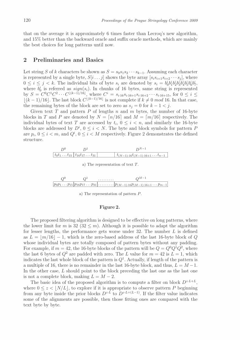
120 Proceedings of the Prague Stringology Conference 2009
that on the average it is approximately 6 times faster than Lecroq’s new algorithm,and 15% better than the backward oracle and suffix oracle methods, which are mainlythe best choices for long patterns until now.
2 Preliminaries and Basics
Let string S of k characters be shown as S = s0s1s2 · · · sk−1. Assuming each characteris represented by a single byte, S[i . . . j] shows the byte array [sisi+1si+2 · · · sj], where0 ≤ i ≤ j < k. The individual bits of byte si are denoted by si = bi
0bi1b
i2b
i3b
i4b
i5b
i6b
i7,
where bi0 is referred as sign(si). In chunks of 16 bytes, same string is represented
by S = C0C1C2 · · ·C⌊(k−1)/16⌋, where Ci = si·16si·16+1si·16+2 · · · si·16+15, for 0 ≤ i ≤⌊(k − 1)/16⌋. The last block C⌊(k−1)/16⌋ is not complete if k 6= 0 mod 16. In that case,the remaining bytes of the block are set to zero as sj = 0 for k − 1 < j.
Given text T and pattern P of lengths n and m bytes, the number of 16-byteblocks in T and P are denoted by N = ⌈n/16⌉ and M = ⌈m/16⌉ respectively. Theindividual bytes of text T are accessed by ti, 0 ≤ i < n, and similarly the 16-byteblocks are addressed by Di, 0 ≤ i < N . The byte and block symbols for pattern Pare pi, 0 ≤ i < m, and Qi, 0 ≤ i < M respectively. Figure 2 demonstrates the definedstructure.
D0 D1 DN−1
t0t1 . . . t15 t16t17 . . . t31 t(N−1)·16t(N−1)·16+1 . . . tn−1
a) The representation of text T .
Q0 Q1 . . . . . . . . . QM−1
p0p1 . . . p15 p16p17 . . . p31 . . . . . . . . . p(M−1)·16p(M−1)·16+1 . . . pm−1
a) The representation of pattern P .
Figure 2.
The proposed filtering algorithm is designed to be effective on long patterns, wherethe lower limit for m is 32 (32 ≤ m). Although it is possible to adapt the algorithmfor lesser lengths, the performance gets worse under 32. The number L is definedas L = ⌊m/16⌋ − 1, which is the zero-based address of the last 16-byte block of Qwhose individual bytes are totally composed of pattern bytes without any padding.For example, if m = 42, the 16-byte blocks of the pattern will be Q = Q0Q1Q2, wherethe last 6 bytes of Q2 are padded with zero. The L value for m = 42 is L = 1, whichindicates the last whole block of the pattern is Q1. Actually, if length of the pattern isa multiple of 16, there is no remainder in the last 16-byte block, and thus, L = M−1.In the other case, L should point to the block preceding the last one as the last oneis not a complete block, making L = M − 2.
The basic idea of the proposed algorithm is to compute a filter on block Dz·L+L,where 0 ≤ z < ⌊N/L⌋, to explore if it is appropriate to observe pattern P beginningfrom any byte inside the prior blocks Dz·L to Dz·L+(L−1). If the filter value indicatessome of the alignments are possible, then those fitting ones are compared with thetext byte by byte.

M. O. Kulekci: Filter Based Fast Matching of Long Patterns by Using SIMD Instructions 121
Figure 3 demonstrates this basic idea by assuming i = z ·L. Note that as m ≥ 32,and L = ⌊m/16⌋ − 1, the pattern fills the bytes in Di+L always.
Block No Di Di+1 . . . . . . . . . Di+L−1 Di+L
Bytes of T ti·16 . . . . . . . . . t(i+1)·16 . . . . . . . . . . . . t(i+L−1)·16 . . . t(i+L)·16 . . . t(i+1)·16+15
P aligned to ti·16 p0 . . . . . . . . . p16 . . . . . . . . . . . . p(L−1)·16 . . . pL·16 . . . pL·16+15
P aligned to ti·16+1 p0 . . . . . . p15 . . . . . . . . . . . . p(L−1)·16−1 . . . pL·16−1 . . . pL·16+14
. . . . . . . . . . . . . . . . . . . . . . . . . . . . . . . . . . . . . . . . . . . . . . . . . . . . . . . . . . . . . . . . . .
P aligned to ti·16+15 . . . . . . . . . p0 p1 . . . . . . . . . . . . p(L−1)·16−15 . . . pL·16−15 . . . pL·16
. . . . . . . . . . . . . . . . . . . . . . . . . . . . . . . . . . . . . . . . . . . . . . . . . . . . . . . . . . . . . . . . . .
P aligned to t(i+L)·16−1 p0 p1 . . . p16
Figure 3. Appropriate alignments of pattern P according to the filter value computedfrom Di+L,for any i = z · L
3 The SSEF Exact Pattern Matching Algorithm
3.1 Preprocessing
The preprocessing stage of the algorithm consist of compiling the possible filter valuesof the pattern according to the alignments shown in figure 3. Formally, the filtervalues for P [(L · 16) . . . (L · 16 + 15)], P [(L · 16− 1) . . . (L · 16 + 14)], . . . , P [1 . . . 16]are computed and stored in a linked list, which will be referred as FList from nowon. The pseudo-code of the preprocessing procedure is depicted in Algorithm 1.
Algorithm 1 PreProcess(P = p0p1p2 · · · pm−1,K)
1: for i = 0 to 65535 do
2: FList[i] = ∅;3: end for
4: L = ⌊m/16⌋ − 15: for i = 0 to L · 16− 1 do
6: r = L · 16− i;7: f = sign(pi << K) · 215 + sign(pi+1 << K) · 214 + · · ·+ sign(pi+15 << K)8: FList[f ] = FList[f ] ∪ i;9: end for
10: return L;
The corresponding filter of a 16 bytes sequence is the 16 bits formed by concatenat-ing the sign bits of each byte after shifting by K bits as shown in line 7 of Algorithm 1.The reason for shifting is to generate a distinguishing filter. For example, when thesearch is to be performed on an English text, the sign bits of bytes are generally 0as in the standard ascii table the printable characters of the language reside in first128, where the sign bits are always 0. If we do not include a shift operation, then thefilter f value will be 0 in all cases, and while passing over the text verification will becalled at each byte. On the other hand, if the text we are searching on is composed ofuniformly distributed random 256 bytes, then there is obviously no need for shifting.

122 Proceedings of the Prague Stringology Conference 2009
Hence, the K value is to be decided depending on the alphabet size and characterdistribution of the text. K should be set to a value that the most informative bit ofthe byte must become the sign bit after shift operation. Thus, detection of the mostinformative bit among the 8 bits of a byte is required for best filtering. This is actuallythe position on which the distribution of the bits among the whole text is close totheir expected values. Note that this requires an additional pass over the whole text,which is not good in practice. A more practical approach may be to consider just thealphabet, and assume the distribution of characters is uniform on the given text. Inthat case, we are left with just the |Σ| bytes, and it is more convenient to decide onthe bit position. As an example, let’s consider pattern matching on an ascii codedplain DNA sequence, where the alphabet is ’a’,’t’,’c’,’g’ having ascii codes 01100001,01110100, 01100011, and 01100111 respectively. The first three bits and the fifth bitare all same. Since the number of 1s and 0s are equal on the sixth and seventh positionsfrom the remaining bits, one of them, say 6th, may be used as the distinguishing bit.Thus, while searching on a DNA sequence, setting K = 5 to move this bit to the signbit position would be a good choice when only the alphabet is considered.
3.2 Main algorithm
The pseudo code given in Algorithm 2 depicts the skeleton of the SSEF . After thepreprocessing stage, the main loop investigates 16-byte blocks of text T in steps ofL. If the filter f computed on Di, where i = z · L + L, and 0 ≤ z < ⌊N/L⌋, is notempty, then the appropriate positions listed in FList[f ] are verified accordingly.
Algorithm 2 SSEF(P = p0p1p2 · · · pm−1, T = t0t1t2 · · · tm−1)1: Set K = a, 0 ≤ a < 8, according to the alphabet;2: i = L =PreProcess(P,K);3: while i < N do
4: f = sign(ti·16 << K) · 215 + sign(ti·16+1 << K) · 214 + · · ·+ sign(ti·16+15 << K)5: for all j ∈ FList[f ] do
6: if P = [t(i−L)·16+j . . . t(i−L)·16+j+m−1] then
7: pattern detected at t(i−L)·16+j ;8: end if
9: end for
10: i = i + L;11: end while
Flist[f ] contains a linked list of integers marking the beginning of the pattern.While investigating the filter on Di, if FList[f ] contains number j, where 0 ≤ j <16·L, the pattern potentially begins at t(i−L)·16+j. In that case, a complete verificationis to be performed between P and [t(i−L)·16+j . . . t(i−L)·16+j+m−1].
Calculating the corresponding filter of Di via SSE intrinsics The computa-tion of the filter f of Di in line 4 of pseudo code given in Alg. 2 is performed by 2SSE2 intrinsic functions as1: tmp128 = mm slli epi64(Di, K);2: f = mm movemask epi8(tmp128);
First instruction shifts the corresponding 16 bytes of the text Di by K bits andstores the result in a temporary 128 bit register aiming not to destruct Di itself.
Second, the instruction mm movemask epi8 returns a 16 bit mask composed of thesign bits of the individual 16 bytes forming the 128 bit value. Figure 4 demonstratesthis function.

M. O. Kulekci: Filter Based Fast Matching of Long Patterns by Using SIMD Instructions 123
Dj
b16·j0 b16·j
1 . . . b16·j7 b16·j+1
0 b16·j+11 . . . b16·j+1
7 . . . . . . b16·j+150 b16·j+15
1 . . . b16·j+157
⇓mm movemask epi8
⇓b16·j0 b16·j+1
0 b16·j+20 . . . b16·j+15
0
Figure 4. The mm movemask epi8 SSE instruction as the filter.
4 Complexity Analysis
The preprocessing stage of the SSEF algorithm requires an additional space to storethe 65536 items of FList linked list. On a 32 bit machine, assuming each node consistof an integer and a next pointer, this makes up a total of 512 KB (= 65536× 8 byte)memory requirement.
The first loop in Algorithm 1 just initializes the FList list, and the second for loopis run L · 16 times during the preprocessing. Thus, time complexity of preprocessingis O(L · 16) that approximates to O(m).
SSEF algorithm investigates the N 16-byte block text T in steps of L blocks.Total number of filtering operations is exactly ⌊N/L⌋. At each attempt, maximumnumber of verification requests is L · 16, since the filter gives information about thatnumber of appropriate alignments of the pattern. This situation can also be viewedfrom figure 3. On the other hand, if the computed filter is empty, then there isobviously no need for verification. The verification cost is assumed to be O(m) withthe brute-force checking of the pattern.
From these facts, the best case complexity is O(⌊N/L⌋), and worst case complexityis O(⌊N/L⌋ · (L · 16) ·m). Remembering the definitions of N and L as N = ⌈n/16⌉,and L = ⌊m/16⌋ − 1, the best/worst time complexities approximately converges toO(n/m) and O(n.m) respectively, which are equivalent to standard Boyer-Moore [3]algorithm.
There are at most L · 16 distinct filter values for any given pattern among thepossible 65536 values. Hence, the probability that the filter computed on Di+L hitsto a non-empty set is L · 16/65536. This indicates that verification will be requestedfor ⌊N/L⌋× (L · 16/65536) times during the whole execution, assuming characters ofthe text is randomly uniform distributed. The average case complexity, being sum ofthe filter computation time and verification computation time, is then O(⌊N/L⌋ +⌊N/L⌋ × (L · 16/65536)×m), which converges to O(n/m + n ·m/65536).
5 Implementation and Experimental Results
The SSEF algorithm is implemented on 64 bit Intel Xeon processor with 3 GB ofmemory. All of the algorithms included in tests are compiled with GNU C compilergcc 4.1.2 with full optimization turned on by -O3 flag.
The SSE instructions used in the study require the source data to be 16-bytealigned for best performance. The cost of misalignment is very high [16,10,11], andspecial attention was paid to make sure that the text is properly aligned. For thatpurpose the input text is loaded to the memory ensuring that it is 16-byte aligned byusing union aggregate with m128i data type introduced by SSE intrinsics as shownin figure 5.

124 Proceedings of the Prague Stringology Conference 2009
typedef union
__m128i* data16;
unsigned char* data;
TEXT;
Figure 5. The TEXT data type defined for 16-byte alignment of data.
The performance of SSEF algorithm is compared with:
– Lecroq’s q-hash algorithm, which is one of the best filtering algorithms [13], withranks q = 3 (3-hash) and q = 8 (8-hash).
– The quick search (QS) of Sunday, which is a fast implementation of standardBoyer-Moore [3].
– The BLIM of Kulekci [12], as this bit-parallel algorithm is not limited with thecomputer word size, and thus can be run on long patterns also.
– Fast variants of backward oracle and suffix oracle matching [1]. BOM2 and BSOM2are especially fast on long patterns.
|Σ| = 256 |Σ| = 1282-bit encoded DNA sequence English text
Len. BLIM 3-hash 8-hash QS BOM2 BSOM2 SSEF BLIM 3-hash 8-hash QS BOM2 BSOM2 SSEF32 11,06 10,69 11,05 10,53 9,46 9,47 12,03 10,38 9,44 9,75 10,05 9,65 10,04 10,8896 12,16 11,11 10,85 11,35 9,03 9,12 9,69 11,24 9,80 9,57 10,36 8,51 8,56 8,74160 13,20 15,14 14,64 16,06 6,60 6,88 6,64 12,50 13,31 12,85 12,56 8,08 8,03 5,95224 14,18 14,33 13,94 15,29 5,09 5,28 4,66 13,72 12,29 12,11 12,20 6,30 6,23 4,21288 15,14 13,87 13,57 14,43 4,12 4,23 3,58 14,89 11,57 11,66 12,03 5,11 5,06 3,21352 16,16 13,32 13,09 13,95 3,45 3,59 2,91 16,06 11,12 11,26 11,66 4,46 4,41 2,58416 17,14 12,81 12,66 13,28 2,96 3,05 2,44 17,22 10,43 10,67 11,32 3,82 3,75 2,17480 18,07 12,30 12,20 12,84 2,56 2,62 2,16 18,43 10,00 10,33 11,19 3,50 3,41 1,80544 19,14 11,87 11,85 12,55 2,22 2,24 1,90 19,53 9,38 9,85 11,05 3,03 3,02 1,62608 20,26 11,58 11,53 12,16 1,93 1,96 1,68 20,34 9,07 9,64 10,62 2,85 2,79 1,45672 21,01 11,33 11,23 11,86 1,69 1,67 1,54 21,26 8,65 9,36 10,39 2,60 2,55 1,34736 22,06 11,14 11,07 11,72 1,52 1,50 1,36 22,16 8,52 9,16 10,00 2,48 2,36 1,21800 23,00 11,00 10,89 11,53 1,37 1,41 1,21 23,22 8,28 9,04 9,91 2,28 2,26 1,13864 23,99 10,78 10,78 11,30 1,31 1,29 1,15 24,01 7,96 8,78 9,51 2,14 2,08 1,06928 25,07 10,76 10,74 11,40 1,20 1,24 1,09 25,05 7,75 8,67 9,28 2,00 1,99 1,01992 26,22 10,66 10,67 11,22 1,19 1,20 0,98 25,92 7,46 8,54 8,99 1,94 1,91 0,901056 27,41 10,62 10,63 11,08 1,16 1,18 0,96 27,16 7,26 8,54 8,97 1,78 1,81 0,921248 30,82 10,48 10,53 10,89 1,10 1,15 0,92 30,44 7,07 8,39 8,37 1,72 1,70 0,841440 34,19 10,40 10,51 10,51 1,11 1,16 0,82 33,75 6,75 8,20 7,93 1,60 1,64 0,801632 38,05 10,42 10,40 10,64 1,16 1,17 0,84 37,20 6,53 8,21 7,67 1,57 1,60 0,761824 41,85 10,49 10,44 10,56 1,22 1,21 0,82 41,35 6,57 8,21 7,72 1,57 1,60 0,752000 47,09 10,40 10,46 10,99 1,28 1,25 0,81 45,84 6,26 8,08 7,62 1,57 1,60 0,76Avg. 27,79 11,27 11,2 11,67 2,33 2,37 2,14 27,4 8,22 9,16 9,36 2,96 2,96 1,94
Table 1. Experimental comparison of algorithms on large alphabets.
Benchmarks are conducted on various text files having small (Σ = 2, 4), medium(Σ = 16, 20), and large (Σ = 128, 256) alphabets. In practice, small alphabetsmimic the nucleic acid sequences, and middle alphabets correspond to biological se-quences with larger blocks such as amino acids or proteins. Large alphabets represent

M. O. Kulekci: Filter Based Fast Matching of Long Patterns by Using SIMD Instructions 125
the case for natural languages, and series of random bytes such as the compressedfiles.
The summary of the data sets2 used in the experiments are given in Table 2.The distribution of characters are randomly uniform on all data sets except the 5th
one, which is a natural language text. Remembering the discussion in section 3, itis enough to consider the character codings of the alphabet while deciding on thevalue of bit shift amount K on test files except the English text. On natural languagetext file, the experiment is repeated for all possible K values as K = 0, . . . , 7. It isobserved that the performances are compatible for K ∈ 3, 4, 5, 7, and significantlyworse on K ∈ 1, 2. Obviously, selecting K = 0 is the worst since it does not includeany distinguishing power on the set of printable ascii characters.
|Σ| Data set Size K-bit shift1 2 Uniformly distributed random sequence of two characters (’a’ and ’b’). 30 MB 62 4 Plain ASCII coded DNA sequence from Manzini’s DNA corpus 21.6 MB 53 16 Uniformly distributed random sequence of 16 characters (’a’ ... ’p’). 30 MB 74 20 Uniformly distributed random sequence of 20 characters (’a’ ... ’t’). 30 MB 75 128 English text from enwik8 corpus. 20 MB 76 256 2-bit encoded DNA sequence from Manzini’s DNA corpus. 22.7 MB 0
Table 2. Test files used in the experiments.
Patterns of length 32 to 2000 are randomly selected from the input text, andsearched via the included algorithms. 100 samples are taken for each length, andeach sample is matched 10 times on the text. The mean user times are recorded bygetrusage function.
Tables 1 and 3 compare the timings of BLIM, 3-hash, 8-hash, QS, BOM2, BSOM2and SSEF for various pattern lengths in milliseconds. Experimental results indicatethat the SSEF algorithm is the clear winner on all tested alphabet sizes and followedby the BOM2 and BSOM2 algorithms, which are actually known to be the fastest oneson long pattern matching. The performance of BOM2 and BSOM2 are quite good,but with the increasing length of the patterns, the SSEF becomes more dominant.The performances of BOM2/BSOM2 and SSEF improves with the increased length,where Lec3 and Lec8 are not very much effected with the length.
Table 4 summarizes the average measured speeds of the algorithms in mega byteper seconds on tested alphabet sizes. Based on the overall speeds depicted in this table,the performance gain is maximum on small alphabets. SSEF is 3.62 and 2.47 timesfaster than its nearest successor on binary alphabet and plain text DNA sequencesrespectively. When medium size alphabets are concerned, it is 40 % faster than thefollowing best. On natural language text, the performance of the BOM2/BSOM2degrades a little bit since the underlying data is not uniform now, and thus, SSEF is50 % more speedy in this case. When timings on 256-byte alphabets are investigated,10 % improvement is observed according to the next best BOM2 algorithm.
SSEF is approximately more than 5 times faster than the q-hash family, which isone of the best representative of filter-then-search algorithms. Note that the speed
2 Manzini’s DNA compression benchmark corpus can be downloaded fromhttp://web.unipmn.it/manzini/dnacorpus.The enwik8.txt file is the subject of the Hutter Prize compression competition, and can be down-loaded from http://prize.hutter1.net

126 Proceedings of the Prague Stringology Conference 2009
|Σ| = 4 |Σ| = 2Plain ascii DNA sequence Randomly uniform sequence of 2 characters
Len. BLIM 3-hash 8-hash QS BOM2 BSOM2 SSEF BLIM 3-hash 8-hash QS BOM2 BSOM2 SSEF32 15,19 10,95 10,54 49,48 16,20 20,56 11,87 37,09 52,06 14,62 212,37 39,52 52,17 16,1796 12,30 11,04 10,40 50,27 10,72 11,71 9,45 19,12 51,98 14,54 218,18 21,27 25,40 13,06160 13,44 12,54 14,06 51,37 15,77 16,30 6,53 20,22 51,67 19,46 224,04 31,59 35,95 8,98224 14,59 12,60 13,42 53,10 12,22 12,53 4,56 21,38 51,88 18,45 223,00 23,60 26,61 6,32288 15,68 12,69 12,99 50,60 10,06 10,21 3,46 22,51 50,74 18,02 213,45 19,04 21,51 4,87352 16,84 12,64 12,65 52,89 8,69 8,81 2,85 23,65 52,40 17,47 225,81 16,20 18,06 4,00416 17,94 12,67 12,03 50,04 7,53 7,66 2,36 24,68 51,86 16,77 218,05 14,13 15,63 3,36480 19,04 12,74 11,62 49,88 6,75 6,83 2,03 25,92 51,53 16,27 222,09 12,61 13,87 2,91544 20,24 12,72 11,25 49,96 6,11 6,12 1,82 26,96 51,48 15,90 218,66 11,43 12,47 2,60608 21,31 12,57 10,92 52,87 5,56 5,65 1,61 28,09 51,17 15,45 221,21 10,50 11,38 2,36672 22,45 12,56 10,70 51,64 5,12 5,14 1,46 29,18 49,81 15,20 216,25 9,77 10,50 2,21736 23,50 12,42 10,47 51,07 4,76 4,78 1,35 30,32 51,23 14,90 215,31 9,16 9,75 1,95800 24,70 12,48 10,16 51,76 4,44 4,45 1,22 31,45 52,17 14,62 220,85 8,59 9,06 1,81864 25,87 12,21 9,98 51,40 4,13 4,20 1,15 32,46 49,82 14,58 216,94 8,19 8,55 1,62928 26,87 12,44 9,98 51,37 3,88 3,91 1,11 33,67 50,32 14,42 219,99 7,76 8,08 1,55992 28,04 12,25 9,80 49,86 3,68 3,70 1,02 34,88 49,84 14,44 204,53 7,38 7,62 1,461056 29,42 12,33 9,74 49,15 3,46 3,50 1,00 36,31 50,32 14,32 217,54 7,07 7,31 1,301248 33,10 12,22 9,56 49,44 2,95 3,04 0,92 39,67 49,15 14,07 210,31 6,14 6,23 1,191440 36,82 12,26 9,35 48,10 2,59 2,68 0,88 43,54 51,81 14,07 215,02 5,41 5,51 1,101632 40,67 12,18 9,16 53,39 2,40 2,46 0,83 47,15 50,50 14,15 228,67 4,82 4,89 1,001824 44,68 12,18 9,18 51,01 2,27 2,27 0,84 51,21 51,56 14,27 223,11 4,42 4,44 0,962000 50,42 12,17 8,96 50,21 2,18 2,37 0,78 57,04 51,08 14,04 214,72 4,16 4,04 0,93Avg. 29,62 12,27 10,31 50,81 5,23 5,48 2,12 36,80 51,01 15,04 218,52 10,47 11,64 2,89
a) Benchmarks on small alphabet sequences.
|Σ| = 20 |Σ| = 16Randomly uniform sequence of 20 characters Randomly uniform sequence of 16 characters
Len. BLIM 3-hash 8-hash QS BOM2 BSOM2 SSEF BLIM 3-hash 8-hash QS BOM2 BSOM2 SSEF32 14,89 14,40 14,60 15,50 13,28 13,50 15,76 15,00 14,46 14,62 16,75 13,32 13,68 16,4096 15,87 15,30 14,48 15,12 12,32 12,47 12,79 16,00 15,34 14,48 16,15 12,48 12,71 13,06160 17,04 19,67 19,37 15,21 10,67 11,10 8,78 17,03 18,89 19,44 15,96 11,79 12,13 9,01224 18,16 19,23 18,50 15,22 8,33 8,66 6,16 18,16 18,61 18,55 16,12 9,26 9,44 6,32288 19,29 18,90 18,02 15,22 6,96 7,21 4,76 19,34 18,48 17,96 16,18 7,57 7,74 4,91352 20,42 18,70 17,38 15,20 6,04 6,21 3,86 20,45 18,30 17,40 16,06 6,39 6,54 3,99416 21,55 18,55 16,83 15,30 5,30 5,48 3,31 21,54 18,30 16,81 16,13 5,53 5,70 3,40480 22,64 18,34 16,20 15,26 4,69 4,92 2,89 22,67 18,17 16,28 15,94 4,84 5,05 2,92544 23,78 18,10 15,78 15,20 4,21 4,40 2,58 23,86 18,02 15,89 16,07 4,34 4,53 2,58608 24,89 17,96 15,39 15,38 3,83 4,06 2,33 24,95 17,90 15,43 16,11 3,98 4,15 2,33672 26,04 17,70 15,14 15,20 3,54 3,71 2,13 26,10 17,76 15,11 16,04 3,64 3,80 2,15736 27,19 17,68 14,86 15,22 3,23 3,43 1,94 27,19 17,54 14,87 15,97 3,38 3,53 1,92800 28,26 17,50 14,56 15,22 3,01 3,14 1,77 28,22 17,54 14,64 16,14 3,14 3,27 1,74864 29,45 17,32 14,52 15,18 2,74 2,96 1,64 29,50 17,42 14,48 16,06 2,97 3,06 1,64928 30,49 17,18 14,49 15,18 2,57 2,98 1,49 30,61 17,29 14,38 16,16 2,84 2,89 1,53992 31,73 17,14 14,31 15,14 2,41 2,65 1,38 31,80 17,26 14,30 16,16 2,69 2,81 1,471056 33,08 17,05 14,23 15,26 2,21 2,37 1,32 33,04 17,23 14,31 16,02 2,54 2,68 1,341248 36,59 16,84 14,17 15,18 1,97 2,08 1,11 36,78 16,96 14,13 16,10 2,30 2,35 1,171440 40,34 16,70 14,06 15,26 1,82 1,86 1,01 40,50 16,85 13,99 16,23 2,11 2,15 1,081632 44,08 16,56 14,04 15,24 1,71 1,81 0,96 44,04 16,86 14,04 16,08 2,00 2,01 1,001824 48,05 16,45 14,08 15,26 1,73 1,76 0,92 48,04 16,54 14,05 16,13 1,92 1,94 1,002000 53,94 16,39 14,09 15,20 1,68 1,80 0,94 53,16 16,51 14,14 16,20 1,93 2,02 0,92Avg. 33,22 17,23 15,04 15,27 3,84 4,00 2,81 33,06 17,20 15,00 16,11 4,13 4,24 2,90
b) Benchmarks on medium alphabet sequences.
Table 3. Experimental comparison of algorithms on small and medium alphabets.

M. O. Kulekci: Filter Based Fast Matching of Long Patterns by Using SIMD Instructions 127
|Σ| BLIM 3-hash 8-hash QS BOM2 BSOM2 SSEF
2 815,24 588,07 1994,18 137,29 2865,06 2577,82 10382,874 729,20 1760,55 2094,16 425,14 4126,17 3939,90 10201,3116 907,38 1744,17 1999,72 1862,76 7269,64 7074,85 10347,0620 903,09 1741,58 1994,93 1965,23 7809,45 7507,04 10659,09128 729,85 2433,05 2182,84 2135,84 6750,49 6748,78 10307,95256 816,72 2015,00 2026,76 1945,14 9749,29 9591,72 10585,84
Table 4. Average speed of the tested algorithms in MB/sec for each |Σ| alphabetsize.
of the proposed algorithm is not much effected with the size or distribution of thealphabet unlike its nearest competitors BOM2 and BSOM2.
6 Conclusion
This study introduced a filter-then-search type pattern matching algorithm for longpatterns benefiting from computers intrinsic SIMD instructions. Using SIMD intrin-sics has not been much addressed in pattern matching, and this study is an initialexploration of designing algorithms according to that technology, which is developingvery fast.
The proposed SSEF algorithm is implemented on Intel’s SSE (version 2) technol-ogy. Experimental benchmarks showed that on every alphabet sizes it is faster thanall competitors included in this study. Considering the orders of magnitude perfor-mance gain on small and medium alphabet sizes, SSEF becomes a strong alternativefor exact matching of long patterns on biological sequences.
The best and worst case time complexities being O(n/m) and O(n·m) respectivelyare identical with the classical Boyer-Moore type algorithms. The main improvementcomes with the average case complexity of O(n ·m/216). Note that the performance ofthe algorithm is independent of the alphabet size (assuming |Σ| > 1), and conductedexperiments proves this empirically also.
References
1. C. Allauzen, M. Crochemore, and M. Raffinot: Factor oracle: A new structure forpattern matching, in Proceedings of SOFSEM’99, vol. 1725 of LNCS, Springer Verlag, 1999,pp. 291–306.
2. R. Baeza-Yates and G. Gonnet: A new approach to text searching. Communications of theACM, 35(10) 1992, pp. 74–82.
3. R. Boyer and J. Moore: A fast string searching algorithm. Communications of the ACM,20(10) 1977, pp. 762–772.
4. C. Charras and T. Lecroq: Handbook of exact string matching algorithms, King’s CollagePublications, 2004.
5. M. Crochemore and W. Rytter: Jewels of stringology, World Scientific Publishing, 2003.6. K. Fredriksson: Faster string matching with super–alphabets, in Proceedings of the 9th In-
ternational Symposium on String Processing and Information Retrieval (SPIRE’2002), LNCS2476, Springer–Verlag, 2002, pp. 44–57.
7. K. Fredriksson and S. Grabowski: Practical and optimal string matching, in Proceed-ings of the 12th International Symposium on String Processing and Information Retrieval(SPIRE’2005), LNCS 3772, Springer–Verlag, 2005, pp. 374–385.

128 Proceedings of the Prague Stringology Conference 2009
8. M. Hassaballah, S. Omran, and Y. Mahdy: A review of SIMD multimedia extensions andtheir usage in scientific and engineering applications. The Computer Journal, 51(6) November2008, pp. 630–649.
9. J. Holub and B.Durian: Fast variants of bit parallel approach to suffix automata. UnpublishedLecture, University of Haifa, April 2005.
10. I. Hurbain and G. Silber: An empirical study of some x86 simd integer extensions, inProceedings of CPC’2006, 12th International Workshop on Compilers for Parallel Computers,Spain, January 9–11 2006.
11. Intel Corporation, Intel Pentium 4 and Intel Xeon Processor Optimization Reference Man-ual, 2001.
12. M. O. Kulekci: A method to overcome computer word size limitation in bit-parallel patternmatching, in Proceedings of 19th International Symposium on Algorithms and Computation,ISAAC’2008, S.-H. Hong, H. Nagamochi, and T. Fukunaga, eds., vol. 5369 of Lecture Notes inComputer Science, Gold Coast, Australia, December 2008, Springer Verlag, pp. 496–506.
13. T. Lecroq: Fast exact string matching algorithms. Information Processing Letters, 102(6)2007, pp. 229–235.
14. G. Navarro and M. Raffinot: Fast and flexible string matching by combining bit-parallelismand suffix automata. ACM Journal of Experimental Algorithms, 5(4) 2000, pp. 1–36.
15. H. Peltola and J. Tarhio: Alternative algorithms for bit-parallel string matching, in LNCS2857, Proceedings of SPIRE’2003, 2003, pp. 80–94.
16. A. Shahbahrami, B. Juurlink, and S. Vassiliadis: Performance impact of misalignedaccesses in simd extensions, in Proceeedings of ASAP’05, IEEE Conference on ApplicationSpesific Systems Architecture Procesors, Washington,DC, USA, 2005, pp. 393–398.
17. S. Wu and U. Manber: Agrep – a fast approximate pattern-matching tool, in Proceedings ofUSENIX Winter 1992 Technical Conference, 1992, pp. 153–162.
18. S. Wu and U. Manber: Fast text searching allowing errors. Communications of the ACM,35(10) 1992, pp. 83–91.

Validation and Decomposition of Partially
Occluded Images with Holes
Julien Allali1, Pavlos Antoniou2, Costas S. Iliopoulos2, Pascal Ferraro1, and ManalMohamed2
1 LaBRI, University of Bordeaux I, UMR5800, 33405 Talence, France2 Dept. of Computer Science, King’s College London, London WC2R 2LS,
England, UK
Abstract. A partially occluded image consists of a set of objects where some may bepartially occluded by others. Validating occluded images distinguishes whether a givenimage can be covered by the members of a finite set of objects, where both the imageand the object range over identical alphabet. The algorithm presented here validates aone-dimensional image x of length n, over a given set of objects all of equal length andeach composed of two parts separated by a transparent hole.
Keywords: valid image, approximate valid image, image decomposition
1 Introduction
In recent studies of repetitive structures of strings, generalized notions of periods havebeen introduced [2]. Here we present practical methods to study the following typeof regularity: we want to “cover” a string using a set of “objects”.These objects may“occlude” each other and may be separated by a hole.
Validating partially occluded images is a classical problem in computer visionand its computational complexity is exponential. An input image is valid, if it canbe composed from a members of a finite set of objects, with some of the appearingobjects being partially occluded by other ones. This problem is also typical in patternrecognition and computer graphics. There is a great number of artificial intelligenceand neural net solutions to this problem.
Validating occluded one dimensional images has been a well studied problem inalgorithm design. Iliopoulos and Simpson [6] focused on the theoretical aspect of theproblem and produced a sequential on-line algorithm for validating occluded one-dimensional images. Furthermore, different aspects of this problem have been studiedand solved by Iliopoulos and Reid. In [5], the authors provided a linear time solutionto the problem in the presence of errors, in [4] they presented an optimal O(log log n)-time algorithm using parallel computation and in [3] solved the problem for discretetwo-dimensional partially occluded images in linear time.
In this paper, we move a step forward, based on the above analyses and we extendthe previous work by considering the validity of a family of images, that we call validimages with holes. In this context, given a set of objects s1, . . . , sk, each composed oftwo parts separated by a small transparent hole, an image x of length n is a validimage with hole, if x is iteratively obtained from a string z = #n by substitutingsubstrings of z by some objects si , for some i ∈ 1..k and a special “background”symbol #. We focus on designing an on-line algorithm for testing images in onedimension for validity, with restricted set of objects, e.g., objects of the same length,that are consisting of two parts separated by a hole of small size.
Julien Allali, Pavlos Antoniou, Costas S. Iliopoulos, Pascal Ferraro, Manal Mohamed: Validation and Decomposition of Partially Occluded Images with
Holes, pp. 129–136.
Proceedings of PSC 2009, Jan Holub and Jan Zd’arek (Eds.), ISBN 978-80-01-04403-2 c© Czech Technical University in Prague, Czech Republic

130 Proceedings of the Prague Stringology Conference 2009
The paper is organized as follows. In Section 2, we introduce basic definitions andnotations used in this paper. In Section 3, we present the principles for validatingimages in one dimension. In Section 4, the main validating algorithm is presentedwith its time complexity analysis. Finally, we state our conclusions in Section 5.
2 Background
An alphabet Σ is a set of elements that are called letters, characters or symbols. Astring x is a sequence of zero or more letters from Σ, that is x[1]x[2] · · · x[n] withx[i] ∈ Σ, 1 ≤ i ≤ n. The length of x, denoted by |x|, is the total number of letters inx. The string of length zero is the empty string ε. The string xy is a concatenationof two strings x and y.
A string y is a substring of x, if and only if, there exist two strings u and v suchthat x = uyv. A string u is a prefix (respectively suffix ) of x, if and only if, thereexists a string v over such that x = uv (respectively x = vu). If v 6= ε then u is aproper prefix (respectively proper suffix ) of x.
Additionally, prefixp(x) denotes the first p letters of x and suffixp(x) denotes thelast p letters of x. Given two strings x = x[1]x[2] · · · x[n] and y = y[1]y[2] · · · y[m],such that x[n − i + 1] · · · x[n] = y[1] · · · y[i] for some i ≥ 1 (that is such that x hasa suffix equal to a prefix of y), the string x[1] · · · x[n]y[i + 1] · · · y[m] is called asuperposition of x and y with i overlap. A string w of x is called a cover of x if andonly if an extension of x can be constructed by concatenations and superposition ofw.
Valid Image over set of Objects:
Definition 1. Let x be a string of length n over an alphabet Σ and let the dictionaryO = s1, . . . , sm be a set of strings called the objects also over Σ. Then x is calleda valid image if and only if x = zi for some i ≥ 0, where
z0 = #n
zi+1 = prefixp(zi) sl suffixq(zi) . (1)
for some sl ∈ O and p, q ∈ 0, . . . , n− 1 such that p + |sm|+ q = n. ⊓⊔Equation (1) is called the substitution rule and the sequence z0, z1, . . .,zi is called thegenerating sequence of x. The number of distinct generating sequences was proved tobe exponential [6].
An example of such generating sequences for a specific string is as follows. LetO = s1 = abc, s2 = acde, s3 = ade, s4 = dc, s5 = abd. Then x = abababacdedcdcadeis a valid image over O with generating sequence:
z0 = #17,
z1 = abc#14,
z2 = abc#11ade,
z3 = ababc#9ade,
z4 = abababc#7ade,
z5 = abababacde#4ade,

J. Allali, P. Antoniou, C. S. Iliopoulos, P. Ferraro, M. Mohamed: Validation and. . . 131
z6 = abababacdedc#2ade,
z7 = abababacdedcdcade.
Note that the generating sequence of x is not unique. The following sequence:
z0 = #17,
z1 = abd#14,
z2 = ababc#12,
z3 = abababc#10,
z4 = abababc#7ade,
z5 = abababc#3dc#2ade,
z6 = abababc#3dcdcade,
z7 = abababacdedcdcade.
also generates x as a valid image over O.
Valid Image over Set of Objects with Hole:Let x be a string of length n over an alphabet Σ and let the dictionary O = s1, . . . , skbe a set of strings called the objects, where each object si is composed of two stringssl
i and sri separated by a hole of length h. Then x is called a valid image if and only
if x = zi for some 0 ≤ i, where
z0 = #n
zi+1 = prefixp(zi) sm suffixq(zi) . (2)
for some sm ∈ O and p, q ∈ 0, . . . , n− 1 such that p + |sm|+ q = n.
Figure 1, presents the notion of finding the objects comprising an image. If theimage is observed from above, one can see some of the objects are partially occludedby others but can see some of the covered ones through the hole. We are trying todecompose what the eye sees to its sources. In this example of Figure 1 the validimage of the objects is composed of the following elements:Image = prefix (sl
2) sl1 suffix (sl
3) substring(sl4) prefix (sr
2) sr1 suffix (sr
3) suffix (sr4)
image x
sl1
sr1
sl2
sr2
sl3
sr3
sl4
sr4
Figure 1. Image consisting from objects separated by a hole of same length.

132 Proceedings of the Prague Stringology Conference 2009
In this paper, we consider the problem of validation of an image over a set ofobjects with holes. Each object si ∈ O consists of a left part (head) and a rightpart(tail) separated by a transparent hole of length h. We denote the left part of si assl
i and the the right part as sri . For simplicity, we require that |sl
i| = |sri | and h≪ |sl
i|,for each si ∈ O.
The definition of a valid image implies that constituent objects are containedwithin the image x. That is, there is no si for all i ∈ 1, . . . , k that is ‘cut’ at x[1]or x[n].
This leads to the following facts:
If x is a valid image over O = s1, s2, . . . , sk, then for some i ∈ 1, . . . , k,Fact 1: there exists a suffix sr
i of sri that is also a suffix of x.
Fact 2: there exists a prefix sli of sl
i that is also a prefix of x.
Fact 3: there is no suffix of a left part sli that occurs in x ending at position ℓ, where
ℓ > n− h− |sri |.
Fact 4: there is no prefix of a right part sri that occurs in x at position ℓ′, where
ℓ′ < |sli|+ h.
3 Validation of Images with Objects of Equal Length
In this section, we start by defining what part of a valid image one should expect tosee within the hole i.e. between the left and the right parts of an object. Subsequently,we proceed and present the main mechanism for validating one-dimensional imagesover a set of objects with holes.
Given a set of objects O, a string b of length h is a binding if it is a concatenationof the following three (possibly empty) parts:
Part 1: is a sequence of suffixes of left/right parts of objects in O,where the leading (first) suffix is a suffix of a left part of an object.
Part 2: is a substring of a left/right part of an object.
Part 3: is a sequence of prefixes of left/right parts of objects in O,where the leading (last) prefix is a prefix of a right part of an object.
Note that any substring of a left or a right part of an object is also a binding ifit is of length h. A binding b is satisfied, if and only if, the length of the part of thevalid image following the binding is big enough to insure that each object from Oappears within the hole is totally occluded by the image.
Theorem 2. Let x be a string over Σ. Let O = s1, s2, . . . , sk be a set of objects allof the same length and each composed of left part sl
i and right part sri separated by a
hole of length h. The string x is a valid image over O if and only if
x = sliy with i ∈ 1..k, (3)

J. Allali, P. Antoniou, C. S. Iliopoulos, P. Ferraro, M. Mohamed: Validation and. . . 133
or
x = ysri with i ∈ 1..k, (4)
or
x = ysiw with i ∈ 1..k, (5)
or
x = yslibs
ri z with i ∈ 1..k, (6)
where sli, sr
i and si denote a prefix of the left part sli, suffix of the right part sr
i and asubstring of either parts of si respectively, y and w are valid images and b is a satisfiedbinding.
The above theorem provides the main mechanism for validating images over aset of objects with holes and all of equal length. Equations (3) and (4) are restate-ments of Facts 1 and 2. Equations (5) and (6) state what one should expect at thedecomposition of two valid sub-images.
If an image x is of the form (5), and si = usiv for some strings u, v and a non-empty substring si of either the left or the right part of si, then x is a valid image,since x can be generated by the sequence:
z0 = #n, z0 = #psi#q, where p = |y| − |u|,
followed by an application of the generating sequence of y on the first |y| symbols ofz1 and the generating sequence of w on the last |w| symbols of z1.
If an image x is of the form (6), and sli, and sr
i are both the left and the right partof si separated by a hole of length h, then x is a valid image, since x can be generatedas:
zi+1 = prefix (zi)slibs
ri suffix (zi),
where b is the part of zi appearing in the hole separating the left and the rightpart of si, followed by an application of the generating sequence of y on the first|y| = |prefix (zi)| + |sl
i| − |sli| symbols of z1 and the generating sequence of w on the
last |w| symbols of z1.
4 An On-Line Algorithm
Here we present the algorithm for validating an image over a set of objects with holesand of equal length. Algorithm 1 presents the main commands of the algorithm inthe form of pseudocode.

134 Proceedings of the Prague Stringology Conference 2009
Algorithm 1 On-line Image Validation ALgorithmInput: image x[1. . . . , n], the set of objects O = s1, s2 . . . sk all of equal length.Output: T if and only if x is a valid image, F otherwise.
initialization
1: valid[0, . . . , n]← [T, F, . . . , F]2: p valid[0]← 13: last prefix← last valid← 04: begin5: for i = 1 to N do
6: do7: p valid[i]← last valid
case study
8: (1) slj = x[ℓ..i] is the longest prefix of some sl
j
9: if valid[ℓ− 1] = T OR prefix[ℓ − 1] = T then
10: prefix[maxlast prefix + 1, ℓ . . . i]← T
11: end if
12: if x[p valid[ℓ− 1] + 1 . . . ℓ− 1] is a substring of some sj ∈ O then
13: prefix[maxlast prefix + 1, ℓ . . . i]← T
14: end if
15: if p valid[ℓ− 1] ≥ ℓ− |sj | − 1 then
16: Return “Invalid Image”17: end if
18: last prefix← i19: (2) sr
j = x[ℓ..i] is the longest prefix of some srj .
20: if prefix[ℓ− 1] = T and first prefix ≤ ℓ− h + |srj | then
21: prefix[maxlast prefix + 1, ℓ . . . i]← T
22: end if
23: if srj = sr
j then
24: valid[i]← T
25: last valid← i26: end if
27: if l suffix[j][ℓ − h− 1] = T and x[ℓ− h..ℓ− 1] is a satisfied binding then
28: prefix[maxlast prefix + 1, ℓ . . . i]← T
29: end if
30: if sj = sj then
31: valid[i]← T
32: last valid← i33: end if
34: (3) slj = x[ℓ..i] is the largest suffix of some sl
j .35: l suffix[j][i] ← T
36: (4) srj = x[ℓ..i] is the largest suffix of some sr
j .37: if p valid[i] ≥ ℓ− 1 then
38: valid[i]← T
39: last valid← i40: end if
41: end for
The algorithm is based on Facts 1-4 as well as the following principles:
(a) The occurrence of a proper prefix of either a left or a right part of an object ina valid image must be followed by a prefix (not necessarily proper) of a left or aright part of an object.
(b) If the occurrence of a proper prefix of either a left or a right part of an object isfollowed by an occurrence of a proper suffix of either a left or a right part of anobject, then the image is not valid. In a valid image, the occurrence of a propersuffix of an object is always preceded by the suffix of either a left or a right partof an object.
(c) The occurrence of a suffix of either a left or a right part of an object can befollowed by either a prefix or a substring or a suffix.

J. Allali, P. Antoniou, C. S. Iliopoulos, P. Ferraro, M. Mohamed: Validation and. . . 135
(d) If an occurrence of a suffix of a left part of an object is not followed by eitheran occurrence of a prefix of its corresponding right part in a distance h or anoccurrence of a prefix of a left part of an object in a distance at most h, then theimage is not valid. In both cases a satisfied binding should separate the two parts.
(e) The occurrence of a substring in a valid image may be preceded by and followedby valid images.
Preprocessing StageIn this stage we preprocess the set of objects. We compute the suffix tree of the setof the left and right parts of all objects in O [7,9,8]. This data structure will allowus to perform a constant time on-line checks whether a suffix, or a substring of sl
j/srj
occurs in any position of x. We will also build the Aho-Corasick automaton [1] forthe set of the left and right parts of all objects in O that will allow us to computethe largest prefixes of sl
j/srj occurring in x.
Main AlgorithmAt the beginning of step i the algorithm has already determined whether x[1..j] is avalid image or not, for all j ∈ 1..i − 1. Moreover, the algorithm should determineby the end of the current step whether x[1..j] is valid or not for j ∈ 1..i. This isachieved by examining the suffixes of x[1..i]. There are six possible cases: A suffix ofx[1..i] can be either a prefix of a left part, a prefix of a right part, a suffix of a leftpart, a suffix of a right part, a substring, a binding or a complete part of an objectsj for some j ∈ 1..k. Otherwise, the string is not a valid image (Theorem 2).
Let slj = x[ℓ..i] be the longest prefix of a left part of an object in O that is also a
suffix of x[1..i]. A prefix of a left part of an object is preceded by either a valid image,or a proper prefix of left/right part an object or a substring of an object.
– If valid[ℓ−1] is marked TRUE, then x[1..ℓ−1] is a valid image and position ℓ couldbe the beginning of a valid sub-image, thus we mark prefix[i] = TRUE, first-prefix= ℓ and last-prefix = i.
– If prefix[ℓ − 1] is marked TRUE, then we have a chain of prefixes, thus we markprefix[i] = TRUE and last-prefix = i.
– If there is no prefix of a left/right part of an object or a valid image preceding slj,
then x[1..i] is valid if and only if x[previous-valid[ℓ− 1] + 1..ℓ− 1] is a substring ofleft/right part of an object or x[previous-valid[ℓ−1]+1..i] is a prefix of a satisfiedbinding. If x[previous-valid[ℓ− 1] + 1..ℓ− 1] is a substring then ℓ is the start of avalid image.
Let srj = x[ℓ..i] be the longest prefix of a right part of an object in O that is also
a suffix of x[1..i]. Similarly, a prefix of an object is preceded by either a proper prefixof left/right part an object or a substring of an object.
– If prefix[ℓ − 1] is marked TRUE and first-prefix ≤ ℓ − h + |srj | , then we have a
chain of prefixes thus we mark prefix[i] = TRUE and last-prefix = i. If srj = sr
j (acomplete left part), then x[1..i] is a valid image and we mark the relevant arrayas TRUE.
– If l-suffix[j][ℓ − h − 1] is marked TRUE and x[ℓ − h..ℓ − 1] is a satisfied bindingthen we have a prefix of a valid image (Eq. (6)), thus we mark prefix[i] = TRUEand last-prefix = i. If sr
j = srj (a complete left part), then x[1..i] is a valid image
and we mark the relevant array as TRUE.
136 Proceedings of the Prague Stringology Conference 2009
Let slj = x[ℓ..i] be the longest suffix of a left part of an object in O that is also a
suffix of x[1..i]. If valid[ℓ− 1] then l-suffix[j][i] is marked TRUE.Finally, let sr
j = x[ℓ..i] be the longest suffix of a right part of an object in O thatis also a suffix of x[1..i]. Note that, in a valid image, a suffix sr
j is always preceded bya valid image.
– If previous-valid[ℓ− 1] ≥ ℓ− 1, then x[1..i] is valid.– If there is no valid image preceding sr
j , then x[1..i] is valid if and only if the lengthof i−previous-valid[ℓ− 1] < |sj|.
Theorem 3. Algorithm 1 validates an image x over a set O of objects of equal lengthand all and each composed of two parts separated by a hole in linear O(|x|+ |O|) time.
Proof. The construction of the Aho-Corasick automaton and the suffix tree of thedictionary O both require O(|O)| time.
At Stage i, finding the largest suffix that is a prefix of some part of an objectrequires constant time. At Stage i−1, we have traced on the Aho-Corasick automatonthe largest prefix of a part of an object that is a suffix of x[1..i − 1]; on Stage i, wecan either extend this prefix with one symbol, x[i], or we can follow the failure linkthat lead to the largest such prefix. Each of the other lines of Algorithm 1 requiresconstant time and thus the bound on the running time follows.
5 Conclusions
We have presented an on-line algorithm that determines whether a given image isvalid or not over a given set of objects with holes where each object composed of twoparts separated by a transparent hole. We have solved the problem for a restricted setof objects. I.e. objects of the same lengths and presented a linear time algorithm. Asfuture work, the algorithm may be modified in the same way as the original validationalgorithm by [6], in order to deal with a set of objects of different lengths. Anotherinteresting problem is the computation of the depth of an object in an image, i.e. thenumber of rules applied after the placement of an object in an image.
References
1. A. V. Aho and M. J. Corasick: Efficient string matching: an aid to bibliographic search.Commun. ACM, 18(6) 1975, pp. 333–340.
2. C. S. Iliopoulos and L. Mouchard: Quasiperiodicity and string covering. Theoretical Com-puter Science, 218(1) 1999, pp. 205–216.
3. C. S. Iliopoulos and J. F. Reid: Validating and decomposing partially occluded two-dimensional images, in Proc. Prague Stringology Club Workshop (PSCW’98), J. Holub andM. Simanek, eds., 1998, pp. 83–94.
4. C. S. Iliopoulos and J. F. Reid: Optimal parallel analysis and decomposition of partiallyoccluded strings. Parallel Computing, 26(4) 2000, pp. 483–494.
5. C. S. Iliopoulos and J. F. Reid: Decomposition of partially occluded strings in the presenceof errors. International Journal of Pattern Recognition and Artificial Intelligence, 15(7) 2001,pp. 1129–1142.
6. C. S. Iliopoulos and J. Simpson: On line validation and analysis of partially occluded images.Journal of Automata, Languages and Combinatorics, 6(3) 2001, pp. 291–303.
7. E. M. McCreight: A space-economical suffix tree construction algorithm. J. ACM, 23(2) 1976,pp. 262–272.
8. E. Ukkonen: On-line construction of suffix trees. Algorithmica, 14(3) 1995, pp. 249–260.9. P. Weiner: Linear pattern matching algorithms, in SWAT ’73: Proceedings of the 14th Annual
Symposium on Switching and Automata Theory (swat 1973), Washington, DC, USA, 1973, IEEEComputer Society, pp. 1–11.

Compressing Bi-Level Images by Block Matching
on a Tree Architecture
Sergio De Agostino
Computer Science DepartmentSapienza University
Via Salaria 113, 00198 Roma, [email protected]
Abstract. A work-optimal O(log M log n) time parallel implementation of lossless im-age compression by block matching of bi-level images is shown on a full binary treearchitecture under some realistic assumptions, where n is the size of the image and Mis the maximum size of the match. Decompression on this architecture is also possi-ble with the same parallel computational complexity. Such implementations have noscalability issues.
Keywords: lossless compression, sliding dictionary, bi-level image, tree architecture
1 Introduction
Storer suggested that fast encoders are possible for two-dimensional lossless compres-sion by showing a square greedy matching heuristic for bi-level images, which canbe implemented by a simple hashing scheme [6]. Rectangle matching improves thecompression performance, but it is slower since it requires O(M log M) time for asingle match, where M is the size of the match [7]. Therefore, the sequential time tocompress an image of size n by rectangle matching is Ω(n log M).
The technique is a two-dimensional extension of LZ1 compression [5]. Simple andpractical heuristics exist to implement LZ1 compression by means of hashing tech-niques [2], [9], [10]. The hashing technique used for the two-dimensional extension iseven simpler.
Among the different ways of reading an image, we assume that the rectanglematching compression heuristic is scanning an m × m′ image row by row (rasterscan). A 64 K table with one position for each possible 4 × 4 subarray is the onlydata structure used. All-zero and all-one rectangles are handled differently. The en-coding scheme is to precede each item with a flag field indicating whether there is amonochromatic rectangle, a match, or raw data. When there is a match, the 4 × 4subarray in the current position is hashed to yield a pointer to a copy. This pointeris used for the current rectangle greedy match and then replaced in the hash table bya pointer to the current position. As mentioned above, the procedure for computingthe largest rectangle match with left upper corners in positions (i, j) and (k, h) takesO(M log M) time, where M is the size of the match. This procedure can be used forcomputing the largest monochromatic rectangle in a given position (i, j) as well. Ifthe 4 × 4 subarray in position (i, j) is monochromatic, then we compute the largestmonochromatic rectangle in that position. Otherwise, we compute the largest rect-angle match in the position provided by the hash table and update the table withthe current position. If the subarray is not hashed to a pointer, then it is left uncom-pressed and added to the hash table with its current position. The positions covered
Sergio De Agostino: Compressing Bi-Level Images by Block Matching on a Tree Architecture, pp. 137–145.
Proceedings of PSC 2009, Jan Holub and Jan Zd’arek (Eds.), ISBN 978-80-01-04403-2 c© Czech Technical University in Prague, Czech Republic

138 Proceedings of the Prague Stringology Conference 2009
by matches are skipped in the linear scan of the image and the sequential time tocompress an image of size n by rectangle matching is Ω(n log M). We want to pointout that besides the proper matches we call a match every rectangle of the parsing ofthe image produced by the heuristic. We also call pointer the encoding of a match.
The analysis of the running time of these algorithms involve a so called wastefactor, defined as the average number of matches covering the same pixel. In [7], itis conjectured that the waste factor is less than 2 on realistic image data. Therefore,the square greedy matching heuristic takes linear time while the rectangle greedymatching heuristic takes O(n log M) time. On the other hand, the decoding algorithmsare both linear.
Parallel coding and decoding algorithms were shown in [3] requiring O(log M log n)time and O(n/ log n) processors on the PRAM EREW, mesh of trees, pyramidal, andmultigrid architectures. The parallel encoder and decoder on the pyramid and themultigrid require some realistic assumptions. Under the same realistic assumptions,we show in this paper how to implement such encoder/decoder with the same par-allel complexity on a full binary tree architecture. In section 2, we explain the blockmatching heuristic. In section 3, we describe scalable algoritms for coding and de-coding bi-level images compressed by block matching on an exclusive read, exclusivewrite shared memory parallel machine. In section 4, we show how such parallel imple-mentations can be run on a tree architecture. Conclusions and future work are givenin section 5.
2 The Block Matching Heuristic
The compression heuristic scans an image row by row. We denote with pi,j the pixel inposition (i, j). The procedure for finding the largest rectangle with left upper corner(i, j) that matches a rectangle with left upper corner (k, h) is described in figure 1.
w = k;
r = i;
width = m;
length = 0;
side1 = side2 = area = 0;
repeat
Let p
r;j
p
r;j+`1
be the longest mat h in (w;h) with ` width;
length = length+ 1;
width = `;
r = r + 1;
w = w + 1;
if (length width > area) f
area = length width;
side1 = length;
side2 = width;
g
until area width (i k + 1) or w = i+ 1
Figure 1. Computing the largest rectangle match in (i, j) and (k, h).

S. De Agostino: Compressing Bi-Level Images by Block Matching on a Tree Architecture 139
At the first step, the procedure computes the longest possible width for a rectanglematch in (i, j) with respect to the position (k, h). The rectangle 1 × ℓ computed atthe first step is the current rectangle match and the sizes of its sides are stored inside1 and side2. In order to check whether there is a better match than the currentone, the longest one-dimensional match on the next row and column j, not exceedingthe current width, is computed with respect to the row next to the current copy andto column h. Its length is stored in the temporary variable width and the temporaryvariable length is increased by one. If the rectangle R whose sides have size widthand length is greater than the current match, the current match is replaced by R.We iterate this operation on each row until the area of the current match is greateror equal to the area of the longest feasible width-wide rectangle, since no furtherimprovement would be possible at that point. For example, in figure 2 we apply theprocedure to find the largest rectangle match between position (0, 0) and (6, 6).
0 0 1 0 1 1 0 1 0 0 0 0 1 1 1 step 1
0 0 1 1 1 0 0 1 0 0 0 0 0 1 0 step 2
1 0 1 1 1 0 0 1 0 1 0 0 1 1 1 step 3
0 1 1 0 1 1 0 0 0 0 0 0 0 1 1 step 4
0 1 1 0 1 0 0 1 0 0 0 0 0 0 1 step 5
0 0 0 0 1 1 0 1 1 0 0 0 1 1 1 step 6
0 0 1 0 1 1 0 0 1 0 1 1 1 1 1 step 1
0 0 1 0 1 1 0 0 1 1 0 0 1 1 1 step 2
0 0 1 0 1 1 1 0 0 0 0 0 1 1 1 step 3
0 0 1 0 1 1 0 1 0 0 0 0 1 1 1 step 4
0 0 1 0 1 1 0 1 0 0 0 0 1 1 1 step 5
0 0 1 0 1 1 0 1 0 0 0 0 1 1 1 step 6
0 0 0 0 1 1 0 1 1 0 0 0 1 1 1
Figure 2. The largest match in (0,0) and (6,6) is computed at step 5.
A one-dimensional match of width 6 is found at step 1. Then, at step 2 a bettermatch is obtained which is 2× 4. At step 3 and step 4 the current match is still 2× 4since the longest match on row 3 and 9 has width 2. At step 5, another match ofwidth 2 provides a better rectangle match which is 5 × 2. At step 6, the procedurestops since the longest match has width 1 and the rectangle match can cover at most7 rows. It follows that 5× 2 is the greedy match since a rectangle of width 1 cannothave a larger area. Obviously, this procedure can be used for computing the largestmonochromatic rectangle in a given position (i, j) as well.
As mentioned in the introduction, the procedure for computing the largest rect-angle match takes O(M log M) time, where M is the size of the match. The positionscovered by matches are skipped in the linear scan of the image and the sequentialtime to compress an image of size n by rectangle matching is Ω(n log M). The anal-ysis of the running time of this algorithm involve a so called waste factor, defined asthe average number of matches covering the same pixel. In [7], it is conjectured that

140 Proceedings of the Prague Stringology Conference 2009
the waste factor is less than 2 on realistic image data. Therefore, the square greedymatching heuristic takes linear time while the rectangle greedy matching heuristictakes O(n log M) time. On the other hand, the decoding algorithms are both linear.
3 A Massively Parallel Block Matching Algorithm
Coding and decoding algorithms are shown in [3] on the PRAM EREW, mesh of trees,pyramidal, and multigrid architectures, requiring O(log M log n) time and O(n/ log n)processors. The pyramid and multigrid implementations need some realistic assump-tions. Under the same realistic assumptions, we show in the next section how toimplement such encoder/decoder with the same parallel complexity on a full binarytree architecture. In this section, we present the PRAM EREW encoder/decoder.These algorithms can be implemented in O(α log M) time with O(n/α) processorsfor any integer square value α ∈ Ω(log n).
To achieve sublinear time we partition an m ×m′ image I in x × y rectangularareas, where x and y are Θ(α1/2). In parallel for each area, one processor applies thesequential parsing algorithm so that in O(α log M) time each area will be parsed inrectangles, some of which are monochromatic. Before encoding we wish to computelarger monochromatic rectangles.
3.1 Computing the Monochromatic Rectangles
We compute larger monochromatic rectangles by merging adjacent monochromaticareas without considering those monochromatic rectangles properly contained in somearea. Such limitation has no relevant effect on the compression ratio.
We denote with Ai,j for 1 ≤ i ≤ ⌈m/x⌉ and 1 ≤ j ≤ ⌈m′/y⌉ the areas into whichthe image is partitioned. In parallel for 1 ≤ i ≤ ⌈m/x⌉, if i is odd, a processor mergesareas A2i−1,j and A2i,j provided they are monochromatic and have the same color. Thesame is done horizontally for Ai,2j−1 and Ai,2j. At the k-th step, if areas A(i−1)2k−1+1,j,A(i−1)2k−1+2,j, . . . , Ai2k−1,j, with i odd, were merged, then they will merge with areasAi2k−1+1,j, Ai2k−1+2,j, . . . , A(i+1)2k−1,j, if they are monochromatic with the same color.The same is done horizontally for Ai,(j−1)2k−1+1, Ai,(j−1)2k−1+2, . . . , Ai,j2k−1 , with jodd, and Ai,j2k−1+1, Ai,j2k−1+2, . . . , Ai,(j+1)2k−1 . After O(log M) steps, the procedure iscompleted and each step takes O(α) time and O(n/α) processors since there is oneprocessor for each area. Therefore, the image parsing phase is realized in O(α log M)time with O(n/α) processors on an exclusive read, exclusive write shared memorymachine.
3.2 The Parallel Encoder
We derive the sequence of pointers from the image parsing computed above. In O(α)time with O(n/α) processors we can identify every upper left corner of a match(proper, monochromatic, or raw) by assigning a different segment of length Θ(α)on a row to each processor. Each processor detects the upper left corners on itssegment. Then, by parallel prefix we obtain a sequence of pointers decodable by thedecompressor paired with the sequential heuristic. However, the decoding of suchsequence seems hard to parallelize. In order to design a parallel decoder, it is moresuitable to produce the sequence of pointers by a raster scan of each of the areas intowhich the image was originally partitioned, where the areas are ordered by a raster

S. De Agostino: Compressing Bi-Level Images by Block Matching on a Tree Architecture 141
scan themselves. Again we can easily derive the sequence of pointers in O(α) timewith O(n/α) processors by detecting in each area every upper left corner of a matchand producing the sequence of pointers by parallel prefix.
As mentioned in the introduction, the encoding scheme for the pointers uses a flagfield indicating whether there is a monochromatic rectangle (0 for the white ones and10 for the black ones), a proper match (110), or raw data (111). For the feasibilityof the parallel decoder, we want to indicate the end of the encoding of the sequenceof matches with the upper left corner in a specific area. Therefore, we change theencoding scheme by associating the flag field 1110 to the raw match so that we canindicate with 1111 the end of the sequence of pointers corresponding to a given area.Moreover, since some areas could be entirely covered by a monochromatic match 1111is followed by the index associated with the next area by the raster scan. The pointerof a monochromatic match has fields for the width and the length while the pointerof a proper match also has fields for the coordinates of the left upper corner of thecopy in the window. In order to save bits, the value stored in any of these fields isthe binary value of the field plus 1 (so, we employ the zero value). Also, the rangefor these values is determined by α but for the width and length of monochromaticmatches sharing the upper left corner with one of the areas Ai,j (in this case, therange is determined by the width and length of the image). This coding technique ismore redundant than others previously designed, but its compression effectiveness isstill better than the one of the square greedy matching technique.
3.3 The Parallel Decoder
The parallel decoder has three phases. Observe that at each position of the binarystring encoding the image, we read a substring of bits that is either 1111 (recall thatthe k bits following 1111 provide the area index, where k is the number of bits usedto encode it) or can be interpreted as a flag field of a pointer. Then, in the first phasewe reduce the binary string to a doubly-linked structure and apply the Euler tourtechnique in order to identify for each area the corresponding pointers. The reductionworks as follows: link each position p of the string to the position next to the end of thesubstring starting in position p that either is equal to 1111 followed by k bits or canbe interpreted as a pointer. For those suffixes of the string which can be interpretedas pointers, their first positions are linked to a special node denoting the end of thecoding. For those suffixes of the string which cannot be interpreted as pointers, theirfirst positions are not linked to anything. The linked structure is a forest with onetree rooted in the special node denoting the end of the coding and the other treesrooted in the first position of a suffix of the encoding string not interpretable as apointer. The first position of the binary string is a leaf of the tree rooted in thespecial node. The sequence of pointers encoding the image is given by the path fromthe first position to the root. In order to compute such path we need the children tobe doubly-linked to the parent. Then, we need to reserve space for each node to storethe links to the children. Each node has at most five children since there are onlyfour different pointer sizes (white, black, raw, or proper match). So, for each positionp of the binary sequence we set aside five locations [p, 1], . . . , [p, 5], initially set tozero. When a link is added from position p′ to p, depending on whether the substringstarting in position p′ is 1111 or can be interpreted as a pointer to a raw, white,black or proper match, the value p′ is overwritten on location [p, 1], [p, 2], [p, 3] [p, 4]or [p, 5], respectively. The linking for the substrings starting with 1111 is done first,

142 Proceedings of the Prague Stringology Conference 2009
since only afterwards we know exactly which substrings can be interpreted as pointers(recall that encoding the width and length of a monochromatic match sharing theleft upper corner with one of the areas Ai,j depends on the width and length of thewhole image). Then, by means of the well-known Euler technique [8] we can linearizethe linked structure and apply list ranking to obtain the path from the first positionof the sequence to the root of its tree in O(α) time with O(n/α) processors on anexclusive read, exclusive write shared memory machine [1], [4], since the row imagesize is greater than the size of the encoding binary string. Then, still in O(α) timewith O(n/α) processors we can identify the positions on the path corresponding to1111.
In the second phase of the parallel decoder a different processor decodes thesequence of pointers corresponding to a different area. As far as the pointers tomonochromatic matches are considered, each processor decompresses either a matchcontained in an area or the portion of the match corresponding to the left upper area.Therefore, after the second phase an area might not be decompressed. Obviously, thesecond phase requires O(α) time and O(n/α) processors.
The third phase completes the decoding. In the previous subsection, we denotedwith Ai,j for 1 ≤ i ≤ ⌈m/x⌉ and 1 ≤ j ≤ ⌈m′/y⌉ the areas into which the im-age was partitioned by the encoder. At the first step of the third phase, one pro-cessor for each area A2i−1,j decodes A2i,j, if A2i−1,j is the upper left portion ofa monochromatic match and the length field of the corresponding pointer informsthat A2i,j is part of the match. The same is done horizontally for Ai,2j−1 and Ai,2j
(using the width field of its pointer) if it is known already by the decoder thatAi,2j−1 is part of a monochromatic match. Similarly at the k-th step, one proces-sor for each of the areas A(i−1)2k−1+1,j, A(i−1)2k−1+2,j, . . . , Ai2k−1,j, with i odd, de-codes the areas Ai2k−1+1,j, Ai2k−1+2,j, . . . , A(i+1)2k−1,j, respectively. The same is donehorizontally for Ai,(j−1)2k−1+1, Ai,(j−1)2k−1+2, . . . , Ai,j2k−1 , with j odd, and Ai,j2k−1+1,Ai,j2k−1+2, . . . , Ai,(j+1)2k−1 . After O(log M) steps the image is entirely decompressed.Each step takes O(α) time and O(n/α) processors since there is one processor for eacharea. Therefore, the decoder is realized in O(α log M) time with O(n/α) processors.
4 The Tree Architecture Implementations
We implement the parallel BLOCK MATCHING encoder and decoder on a full binarytree architecture. We extend the m×m′ image I with dummy rows and columns sothat I is partitioned into x×y areas Ai,j for 1 ≤ i, j ≤ 2h, where x and y are Θ(α1/2),n = mm′ is the size of the image and h = mink : 2k ≥ maxm/x,m′/y. Westore these areas into the leaves of the tree according to a one-dimensional layoutwhich allows an easy way of merging the monochromatic ones at the upper levels.Let µ = 2h. The number of leaves is 22h and the leaves are numbered from 1 to 22h
from left to right. It follows that the tree has height 2h. Therefore, the height of thetree is O(log n) and the number of nodes is O(n/α). Such layout is described by therecursive procedure of figure 3. The initial value for i, j and ℓ is 1 and ℓ is a globalvariable.
In parallel for each area, each leaf processor applies the sequential parsing algo-rithm so that in O(α log M) time each area is parsed into rectangles, some of which aremonochromatic. Again, before encoding we wish to compute larger monochromaticrectangles.

S. De Agostino: Compressing Bi-Level Images by Block Matching on a Tree Architecture 143
STORE(I, µ, i, j)
if µ > 1
STORE(I, µ/2, i, j)
STORE(I, µ/2, i + µ/2, j)
STORE(I, µ/2, i, j + µ/2)
STORE(I, µ/2, i + µ/2, j + µ/2)
else store Ai,j into leaf ℓ; ℓ = ℓ + 1
Figure 3. Storing the image into the leaves of the tree.
4.1 Computing the Monochromatic Rectangles
After the compression heuristic has been executed on each area, we have to showhow the procedure to compute larger monochromatic rectangles can be implementedon a full binary tree architecture with the same number of processors without slow-ing it down. This is possible by making some realistic assumptions. Let ℓR and wR
be the length and the width of a monochromatic match R, respectively. We definesR = maxℓR, wR. We make a first assumption that the number of monochromatic
matches R with sR ≥ 2k⌈log1/2 n⌉ is O(n/(22k log n)) for 1 ≤ k ≤ h− 1. While com-puting larger monochromatic rectangles, we store in each leaf the partial results onthe monochromatic rectangles covering the corresponding area (it is enough to storefor each rectangle the indices of the areas at the upper left and lower right corners).If i is odd, it follows from the procedure of figure 3 that the processors storing areasA2i−1,j and A2i,j are siblings. Such processors merge A2i−1,j and A2i,j provided theyare monochromatic and have the same color by broadcasting the information throughtheir parent. It also follows from such procedure that the same can be done horizon-tally for Ai,2j−1 and Ai,2j by broadcasting the information through the processors atlevel 2h − 2. At the k-th step, if areas A(i−1)2k−1+1,j, A(i−1)2k−1+2,j, . . . , Ai2k−1,j, withi odd, were merged for w1 ≤ j ≤ w2, the processor storing area A(i−1)2k−1+1,w1
willbroadcast to the processors storing the areas Ai2k−1+1,j, Ai2k−1+2,j, . . . , A(i+1)2k−1,j tomerge with the above areas for w1 ≤ j ≤ w2, if they are monochromatic with thesame color. The broadcasting will involve processors up to level 2h−2k+1. The sameis done horizontally, that is, if Ai,(j−1)2k−1+1, Ai,(j−1)2k−1+2, . . . , Ai,j2k−1 , with j odd,were merged for ℓ1 ≤ i ≤ ℓ2, the processor storing area Aℓ1,(j−1)2k−1+1 will broadcastto the processors storing the areas Ai,j2k−1+1, Ai,j2k−1+2, . . . , Ai,(j+1)2k−1 to merge withthe above areas for ℓ1 ≤ i ≤ ℓ2, if they are monochromatic with the same color. Thebroadcasting will involve processors up to level 2h− 2k.
After O(log M) steps, the procedure is completed. If the waste factor is less than2, as conjectured in [7], we can make a second assumption that each pixel is coveredby a constant small number of monochromatic matches. It follows from this secondassumption that the information about the monochromatic matches is distributed

144 Proceedings of the Prague Stringology Conference 2009
among the processors at the same level in a way very close to uniform. Then, itfollows from the first assumption that the amount of information each processor ofthe tree must broadcast is constant. Therefore, each step takes O(α) time and theimage parsing phase is realized with O(α log M) time and O(n/α) processors.
4.2 The Parallel Encoder
The sequence of pointers is trivially produced by the processors which are leaves of thetree. For the monochromatic rectangles, the pointer is written in the leaf storing thearea at the upper left corner. Differently from the shared memory machine decoder,the order of the pointers is the one of the leaves. Since some areas could be entirelycovered by a monochromatic match, the subsequence of pointers corresponding to agiven area is ended with 1111 followed by the index of the leaf storing the next area todecode. We define a variable for each leaf. This variable is set to 1 if the leaf stores atleast a pointer, 0 otherwise. Then, the index of the next area to decode is computedfor each leaf by parallel suffix computation. Moreover, with the possibility of a paralleloutput the sequence can be put together by parallel prefix. This is, obviously, realizedin O(α) time with O(n/α) processors.
4.3 The Parallel Decoder
We store each encoding of an area in a leaf of the tree. The storing procedure readsthe encoding binary string from left to right. When it finds the substring 1111, thisdenotes the end of the encoding of an area and the next k bits provide the leafindex of the next area where k is the number of bits used to encode it. At this point,each processor at the leaf level completes the second phase of the decoder described insubsection 3.3. Then, the third and last phase of the shared memory machine decoderhas the same parallel computational complexity on the tree architecture with the samerealistic assumptions we made for the coding phase. In conclusion, the decoder takesO(α log M) time on a full binary tree architecture with O(n/α) processors.
5 Conclusions
Parallel coding and decoding algorithms for lossless image compression by blockmatching were shown requiring O(log M log n) time and O(n/ log n) processors ona full binary tree architecture, where n is the size of the image and M is the size ofthe match. The parallel coding algorithm is work-optimal since the sequential timerequired by the coding is Ω(n log M). On the other hand, the parallel decoding al-gorithm is not work-optimal since the sequential decompression time is linear. Theseimplementations have the same performance of the shared memory machine algo-rithms under some realistic assumptions and if we do not consider the input/outputprocess. In [3], with such assumptions these algorithms had been realized on a multi-grid which is the simplest architecture among the ones with small diameter and largebisection width. Such realistic assumptions are that each pixel is covered by a smallconstant number of monochromatic rectangles of the image parsing and that theincreasing of the dimensions of the monochromatic rectangles is proportional to thedecreasing of the number of monochromatic rectangles with such dimensions. We haveshown in this paper that with the assumptions made for the multigrid we can relax onthe requirement of an architecture with large bisection width and design compression

S. De Agostino: Compressing Bi-Level Images by Block Matching on a Tree Architecture 145
and decompression on a two-dimensional architecture such as a full binary tree. Thecommunication cost might be low enough to realize efficient implementations on oneof the available parallel machines since the algorithms are scalable.
References
1. R. P. Brent: The parallel evaluation of general arithmetic expressions. Journal of the ACM,21 1974, pp. 201–206.
2. R. P. Brent: A linear algorithm for data compression. Australian Computer Journal, 19 1987,pp. 64–68.
3. L. Cinque and S. DeAgostino: Lossless image compression by block matching on practicalmassively parallel architectures, in Proceedings Prague Stringology Conference, 2008, pp. 26–34.
4. R. Cole and U. Vishkin: Approximate parallel scheduling. Part I: The basic technique withapplications to optimal parallel list ranking in logarithmic time. SIAM Journal on Computing,17 1988, pp. 148–152.
5. A. Lempel and J. Ziv: A universal algorithm for sequential data compression. IEEE Trans-actions on Information Theory, 23 1977, pp. 337–343.
6. J. A. Storer: Lossless image compression using generalized LZ1-type methods, in ProceedingsIEEE Data Compression Conference, 1996, pp. 290–299.
7. J. A. Storer and H. Helfgott: Lossless image compression by block matching. The Com-puter Journal, 40 1997, pp. 137–145.
8. R. E. Tarjan and U. Vishkin: An efficient parallel biconnectivity algorithm. SIAM Journalon Computing, 14 1985, pp. 862–874.
9. J. R. Waterworth: Data compression system. US Patent 4 701 745, 1987.10. D. A. Whiting, G. A. George, and G. E. Ivey: Data compression apparatus and method.
US Patent 5016009, 1991.

Taxonomies of Regular Tree Algorithms
Loek Cleophas1 and Kees Hemerik2
1 FASTAR/Espresso Research Group, Department of Computer Science,University of Pretoria, 0002 Pretoria, Republic of South Africa,
http://www.fastar.org2 Software Engineering & Technology Group, Department of Mathematics and Computer Science,
Eindhoven University of Technology, P.O. Box 513, 5600 MB Eindhoven, The Netherlands,http://www.win.tue.nl/set
[email protected], [email protected]
Abstract. Algorithms for acceptance, pattern matching and parsing of regular treesand the tree automata used in these algorithms have many applications, includinginstruction selection in compilers, implementation of term rewriting systems, and modelchecking. Many such tree algorithms and constructions for such tree automata appearin the literature, but some deficiencies existed, including: inaccessibility of theory andalgorithms; difficulty of comparing algorithms due to variations in presentation styleand level of formality; and lack of reference to the theory in many publications. Analgorithm taxonomy is an effective means of bringing order to such a field. We reporton two taxonomies of regular tree algorithms that we have constructed to deal withthe deficiencies. The complete work has been presented in the PhD thesis of the firstauthor.
Keywords: tree acceptance, tree pattern matching, tree automata, algorithm tax-onomies
1 Introduction
We consider the field of regular tree languages for ordered, ranked trees.1 This field hasa rich theory, with many generalizations from the field of regular string languages,and many relations between the two [9,10,12,14]. Parts of the theory have broadapplicability in areas as diverse as instruction selection in compilers, implementationof term rewriting systems, and model checking.
We focus on algorithmic solutions to three related problems in the field, i.e. treeacceptance, tree pattern matching and tree parsing. Many such algorithms appear inthe literature, but unfortunately some deficiencies exist, including:
1. Inaccessibility of the theory and algorithms, as they are scattered over the litera-ture and few or no (algorithm oriented) overview publications exist.
2. Difficulty of comparing the algorithms due to differences in presentation style andlevel of formality.
3. Lack of reference to the theory and of correctness arguments in publications ofpractical algorithms.
A taxonomy—in a technical sense made more precise below—is an effective meansof bringing order to such a subject. A taxonomy is a systematic classification of prob-lems and solutions in a particular (algorithmic) problem domain. We have constructedtwo such taxonomies, one for tree acceptance algorithms and one for tree patternmatching ones.
1 An example of such a language as defined by a regular tree grammar can be found in Section 4.
Loek Cleophas, Kees Hemerik: Taxonomies of Regular Tree Algorithms, pp. 146–159.
Proceedings of PSC 2009, Jan Holub and Jan Zd’arek (Eds.), ISBN 978-80-01-04403-2 c© Czech Technical University in Prague, Czech Republic

Loek Cleophas and Kees Hemerik: Taxonomies of Regular Tree Algorithms 147
A few more practical deficiencies existed as well: no large and coherent collec-tion of implementations of the algorithms existed; and for practical applications itwas difficult to choose between algorithms. We therefore designed, implemented, andbenchmarked a highly coherent toolkit of most of these algorithms as well. Taxonomiesalso form a good starting point for the construction of such algorithmic toolkits.
In the past, taxonomies and/or toolkits of this kind have been constructed fore.g. sorting [3,11], garbage collection [17], string pattern matching, finite automataconstruction and minimization [21,22].
In this paper we focus on one of our taxonomies, and comment only briefly onthe other one and on the toolkit. The complete work has been presented in the PhDthesis of the first author [9]. For more details we refer to this thesis and to recentshorter publications [5,6,18].
Section 2 gives a brief introduction to taxonomies as we consider them. In Section 3we outline the structure of our taxonomy of algorithms for tree acceptance and brieflycompare it to the one for tree pattern matching. Afterwards we focus on the one fortree acceptance. Definitions of tree and tree grammar related notions are given inSection 4. The main branches of the taxonomy for tree acceptance are discussedin Sections 5–8. Section 9 briefly discusses some other parts of the work, namely thetoolkit and accompanying graphical user interface and the benchmarking experimentsperformed with them. We end the paper with some concluding remarks in Section 10.
2 Taxonomies
In our technical sense a taxonomy is a means of ordering a set of algorithmic problemsand their solutions. Each node of the taxonomy graph is a pair consisting of (aspecification of) a problem and an algorithm solving the problem. For each (problem,algorithm) pair the set of essential details is determined. In general, there are twokinds of details: problem details, which restrict the problem, and algorithm details,which restrict the algorithm (e.g. by making it more deterministic). The root of thetaxonomy graph contains a high-level algorithm of which the correctness is easilyshown. A branch in the graph corresponds to addition of a detail in a correctnesspreserving way. Hence, the correctness of each algorithm follows from the details onits root path and the correctness of the root.
Construction of an algorithm taxonomy is a bottom-up process. A literature sur-vey of the problem domain is performed to gather algorithms. The algorithms arerephrased in a common presentation style and analyzed to determine their essen-tial details. When two algorithms differ only in a few details, abstracting over thosedetails yields a common ancestor. Repeating this abstraction process leads to themain structure of a taxonomy graph. Considering new combinations of details maylead to discovery of new algorithms. Eventually the taxonomy may be presented in atop-down manner.
Several taxonomies of this kind appear in the literature. Broy and Darlington eachconstructed one of sorting algorithms [3,11]. Jonkers [17] constructed a taxonomy ofgarbage collection algorithms and also developed a general theory about algorithmtaxonomies. Watson [21] applied the method to construct taxonomies for string pat-tern algorithms and for the construction and minimization of finite automata. Bothin subject and in style our work is closest to Watson’s.

148 Proceedings of the Prague Stringology Conference 2009
3 Overview of the Taxonomies of Regular Tree Algorithms
5.3.2
5.3.4
t-acceptor
5.4.2
rf
5.4.4
det
5.5.2
fr
5.5.4
det
5.3.6
match-set
5.7.7
rec
5.7.18
tabulate
5.7.35
filter
5.7.37
tabulate
s-path
S. 5.8
sp-matcher
5.8.1
det
S. 5.8
aca-spm
S. 5.8
drfta-spm
filter
tfilt ifilt sfilt cfilt
Figure 1. Tree acceptance taxonomy. Each node is labeled with its correspondingalgorithm or section (S.) number in [9]. Constructions for tree acceptors used inalgorithms of branch (t-acceptor ) are not depicted. The bottom part of the figureshows the four possible filters that can be used for detail filter.
The tree acceptance (aka language membership, membership) problem as we con-sider it is the following: Given a regular tree grammar and a subject tree, determinewhether the tree is an element of the language defined by the grammar. Figure 1depicts the taxonomy of algorithms we have constructed for this problem. The edgelabels correspond to details, explained in Table 1.
In the taxonomy graph, three main subgraphs can be distinguished. The first sub-graph (detail t-acceptor and below) contains all algorithms based on the corre-spondence between regular tree grammars and finite tree automata. For every regulartree grammar an undirected finite tree automaton can be constructed, which acceptsexactly the trees generated by the grammar. By adding more detail, viz. a direction(detail fr: frontier-to-root or detail rf: root-to-frontier) or determinacy (detail det)more specific constructions are obtained. The acceptance algorithms from this partof the taxonomy are described in more detail in Section 5, while the tree automataconstructions used in them are discussed in Section 6.
The second subgraph (detail match-set and below) contains all algorithms based
on suitably chosen generalizations of the relation S∗⇒ t (where
∗⇒ indicates derivationin zero or more steps (see Section 4), S is the start symbol of the grammar and t isthe subject tree). For each subtree of t, they compute a set of items from which tmay be derived, a so-called match set. Tree t is accepted if and only if its match setcontains S. The algorithms in this subgraph of the taxonomy differ in the item setused and in how the match sets are computed. This part of the taxonomy is describedin more detail in Section 7.

Loek Cleophas and Kees Hemerik: Taxonomies of Regular Tree Algorithms 149
t-acceptor Use a tree automaton accepting the language of a regular tree grammar tosolve the language membership problem.
rf Consider the transition relations of the tree automaton used in an algorithmto be directed in a root-to-frontier or top-down direction.
fr Consider the transition relations of the tree automaton used in an algorithmto be directed in a frontier-to-root or bottom-up direction.
det Use a deterministic version of an automaton.match-set Use an item set and a match set function to solve the tree accep-
tance/language membership problem. Such an item set is derived fromthe productions of the regular tree grammar and the match set functionindicates from which of these items a tree is derivable.
rec Compute match set values recursively, i.e. compute the match set valuesfor a tree from the match set values computed for its direct subtrees.
filter Use a filtering function in the computation of match set function values.Before computing the match set for a tree, such a filtering function is appliedto the match sets of its direct subtrees.
tabulate Use a tabulated version of the match set function (and of the filter functions,if filtering is used), in which a bijection is used to identify match sets byintegers.
s-path Uniquely decompose production right hand sides into stringpaths. Basedon matching stringpaths, production right hand sides and nonterminalsderiving the subject tree can be uniquely determined and tree acceptancecan thus be solved.
sp-matcher Use an automaton as a pattern matcher for a set of stringpaths in a root-to-frontier or top-down subject tree traversal.
aca-spm Use an (optimal) Aho-Corasick automaton as a stringpath matcher anddefine transition and output functions in terms of that automaton.
drfta-spm Use a deterministic root-to-frontier tree automaton as a stringpath matcherand define transition and output functions in terms of that automaton.
Table 1.
The third subgraph (detail sp-matcher and below) contains algorithms basedon the decomposition of items into so-called stringpaths and subsequent use of stringmatching techniques. Based on stringpath matches found, matches of items and henceessentially the match sets mentioned previously are computed for each subtree of t.Section 8 gives a brief explanation of this taxonomy part.
As our focus in this paper is on the tree acceptance taxonomy and the algorithmsand constructions included in it, we do not formally define the tree pattern matchingproblem. Figure 2 shows the taxonomy of tree pattern matching algorithms. Althoughwe do not explicitly give the meaning of the details used, it should be clear that thetaxonomies for tree acceptance and tree pattern matching have much in common.Techniques such as the subset construction, match sets, and stringpaths are used inboth. This is not surprising: the two problems are closely related, and some kindsof tree acceptors can be turned into tree pattern matchers (or vice versa) with littleeffort. The same phenomenon can be observed in acceptors and pattern matchers forstring languages.

150 Proceedings of the Prague Stringology Conference 2009
6.2.5
6.2.7
t-matcher
S. 6.3
rf
S. 6.3
det
6.4.2
fr
6.4.4
det
6.2.9
match-set
6.6.7
rec
6.6.10
tabulate
6.6.13
filter
6.6.15
tabulate
6.2.11
s-path
S. 6.7
sp-matcher
6.7.9
det
S. 6.7.1
aca-spm
S. 6.7.2
drfta-spm
filter
tfilt sfilt ifilt cfilt
Figure 2. Tree pattern matching taxonomy. Each node is labeled with its correspond-ing algorithm or section (S.) number in [9]. Constructions for tree pattern matchersused in algorithms of branch (t-matcher) are not depicted. The bottom part of thefigure shows the four possible filters that can be used for detail filter.
4 Notation and definitions
We use B and N to denote the booleans and the natural numbers. We use notation⟨Set a : R(a) : E(a)
⟩for the set of expressions E(a) for which a satisfies range
predicate R(a).Many of the other notations and definitions we use are related to regular tree
language theory and to a large extent generalizations of familiar ones from regularstring language theory. To aid readers unfamiliar with this theory, we briefly intro-duce the concepts needed in the rest of this paper. Readers may want to consulte.g. [9,10,12,14] for more detail.
Let Σ be an alphabet, and r ∈ Σ 7→ N. Pair (Σ, r) is a ranked alphabet, r is aranking function, and for all a ∈ Σ, r(a) is called the rank or arity of a. (The rankingfunction indicates the number of child nodes a node labeled by a particular symbolwill have.) We use Σn for 0 ≤ n to indicate the subset of Σ of symbols with arity n.
Given a ranked alphabet (Σ, r), the set of ordered, ranked trees over this alphabet,set Tr(Σ, r), is the smallest set satisyfing
1. Σ0 ⊆ Tr(Σ, r), and2. a(t1, . . . , tn) ∈ Tr(Σ, r) for all t1, . . . , tn ∈ Tr(Σ, r), a ∈ Σ such that r(a) = n 6= 0.
As a running example, we assume (Σ, r) to be (a, 2), (b, 1), (c, 0), (d, 0), i.e. con-sisting of symbols a, b, c and d with rank 2, 1, 0 and 0. Trees in Tr(Σ, r) include forexample c, a(b(c), d) and a(a(b(c), c), d).
A regular tree grammar (rtg) G is a 5-tuple (N,Σ, r ,Prods, S) where N andΣ are disjoint alphabets (the nonterminals and terminals), (N ∪ Σ, r) is a rankedalphabet in which all nonterminals have rank 0, Prods ⊆ N × Tr(N ∪ Σ, r) is the

Loek Cleophas and Kees Hemerik: Taxonomies of Regular Tree Algorithms 151
finite set of productions, and S ∈ N (the start symbol). We use LHS and RHS for lefthand side and right hand side (of a production), and use RHS(Prods) for the set ofproduction RHSs.
Given a grammar G, we use ⇒ for a derivation step, in which a nonterminal isreplaced by a corresponding production RHS. The reflexive and transitive closure of
⇒ is denoted by∗⇒. The subset of Tr(Σ, r) derivable from S is denoted L(G). For
technical reasons, we introduce the augmented grammar G′ for a grammar G, definedby G′ = (N ∪ S ′, Σ, r ∪ (S ′, 0),Prods∪ S ′ 7→ S, S ′) where S ′ is a fresh symbol.
In this paper, we assume an example grammar G1 = (N,Σ, r ,Prods, S) with N =S,B, r and Σ as before, and with Prods defined as S 7→ a(B, d), S 7→ a(b(c), B),S 7→ c, B 7→ b(B), B 7→ S, B 7→ d. We assume G to be the correspondingaugmented grammar.
5 Algorithms based on Tree Automata
The first subgraph of the taxonomy deals with algorithms for tree acceptance that arebased on correspondences between regular tree grammars and finite tree automata.The theoretical basis for this correspondence is well-known and generalizes a similarcorrespondence between regular string grammars and finite string automata. To easeunderstanding we briefly outline how the generalization works.
It is well known that the theory of regular tree languages generalizes that of regularstring languages [9,10,12,14]. This is not surprising: any string a0 · · · an−1 can be seenas a special kind of regular tree, viz. one consisting of n unary nodes, each labeledwith a symbol ai of rank 1, closed by a nullary node marked with a symbol of rank 0.Notions from finite automata for strings can be generalized to the tree case as well,although this requires a particular view of such automata. Suppose that a particularstring automaton goes through a state sequence q0, . . . , qn when presented the stringa0 · · · an−1. This means that for each i : 0 ≤ i < n the pair of states (qi, qi+1) must bein the transition relation of symbol ai. We can summarize the transition sequence bythe following alternation of states and symbols: q0a0 · · · an−1qn. In other words, thepositions in the string have been consistently annotated with states q0, . . . , qn. Thelanguage accepted by the automaton can be defined as the set of strings that can beconsistently annotated in this way, such that q0 and qn are initial and final states.
This view can easily be generalized to ordered, ranked trees: each node is anno-tated with a state, and for each node labeled with a symbol a of rank n, the stateq0 assigned to that node and the states q1, . . . , qn of the n direct subnodes should besuch that the tuple (q0, (q1, . . . , qn)) is in the transition relation of symbol a. Notethat this simplifies to (q0, ()) for symbols of rank 0. (Hence, taking a frontier-to-rootor bottom-up view on tree automata, no equivalent for a string automaton’s initialstates is needed; no equivalent for a string automaton’s final states is needed whentaking a root-to-frontier or top-down view.) A tree is accepted by a finite tree au-tomaton if and only if it can be consistently annotated such that the state assignedto the root is a so-called root accepting state. This motivates the following definition:
Definition 1. A (finite) tree automaton (ta) M is a 5-tuple (Q,Σ, r , R,Qra) suchthat Q is a finite set, the state set; (Σ, r) is a ranked alphabet; R = Ra|a ∈ Σ∪Rε
is the set of transition relations (where Rε ⊆ Q×Q and Ra ⊆ Q×Qn, for all a ∈ Σwith r(a) = n); and Qra ⊆ Q is the set of root accepting states.

152 Proceedings of the Prague Stringology Conference 2009
Many important theorems carry over from regular string grammars and automatato the tree case as well. In particular:
Theorem 2. For every regular tree grammar G there exists a tree automaton M suchthat L(G) = L(M).
This theorem justifies the following algorithm as a solution for tree acceptance:
Algorithm 3 (t-acceptor)
|[ const G = (N ′, Σ, r ′,Prods′, S ′) : augmented rtg;t : Tr(Σ, r);
var b : B
| let M = (Q, Σ, r, R, Qra) be a ta such that L(M) = L(G);b : = t ∈ L(M) b ≡ t ∈ L(G)
]|
This abstract and rather trivial algorithm forms the root of the part of the tax-onomy graph containing all algorithms based on tree automata. Note that it doesnot specify how t ∈ L(M) is determined. It could consider all state assignments to trespecting the transition relations R, and determine whether an accepting one exists.
To obtain more specific and more practical algorithms, the automata and hencethe state assignments can be considered as directed ones (detail fr: frontier-to-rootaka bottom-up or detail rf: root-to-frontier aka top-down). This results in (the useof) an ε-nondeterministic frontier-to-root ta (εnfrta) and ε-nondeterministic root-to-frontier ta (εnrfta).
Restricting the directed automata to the case without ε-transitions, we obtain theε-less ta and (ε-less) nrfta and nfrta. As with string automata, ε-transitions canbe removed by a straightforward transformation. The use of the resulting automataslightly simplifies the acceptance algorithms.
5.1 fr: Frontier-to-Root Tree Acceptors
For (ε)nfrtas, a recursive acceptance function RSt ∈ Tr(Σ, r) 7→ P(Q) can bedefined. This function yields the states assigned to a tree’s root node based on thoseassigned to that node’s child nodes. A subject tree t is then accepted if and only ifat least one accepting state occurs in state set RSt(t).
Restricting the directed Ra of the (ε-less) nfrta to be single-valued functions,we obtain the deterministic dfrta. A subset construction subsetfr can be given,similar to that for string automata, to obtain a dfrta for an (ε)nfrta. The use ofa dfrta leads to the straightforward Algorithm 4 given below.

Loek Cleophas and Kees Hemerik: Taxonomies of Regular Tree Algorithms 153
Algorithm 4 (t-acceptor, fr, det)
|[ const G = (N ′, Σ, r ′,Prods′, S ′) : augmented rtg;t : Tr(Σ, r);
var b : B
| let M = (Q, Σ, r, R, Qra) be a dfrta such that L(M) = L(G);b : = Traverse(t) ∈ Qra
b ≡ t ∈ L(G)
func Traverse(st : Tr(Σ, r)) : Q =|[| let a = st(ε); st = a(st1, . . . , stn) where n = r(a) Traverse : = Ra(Traverse(st1), . . . ,Traverse(stn))
]| Post: Traverse = RSt(st) ]|
5.2 rf: Root-to-Frontier Tree Acceptors
For root-to-frontier automata, we can define a root-to-frontier acceptance functionAccept ∈ Tr(Σ, r) × Q 7→ B indicating whether an accepting computation startingfrom some state exists for a tree. In the resulting Algorithm (t-acceptor, rf) (notgiven here), the value of this function is computed by possibly many root-to-frontiersubject tree traversals (starting from each of the root accepting states).
As with frtas, rftas can be restricted to ε-less ones and further to deterministicones. Since drftas are known to be less powerful than other ta kinds, algorithmsusing drftas cannot solve the acceptance problem for each input grammar. We referthe reader to [9] for more information on algorithms using rftas to directly solve thetree acceptance problem.
In Section 8 we briefly discuss how drftas can be used for so-called stringpathmatching. Since there is a one-to-one correspondence between a tree and its set ofstringpaths, drftas can thus be used to solve the tree acceptance problem, albeitindirectly.
6 Construction of tree automata
Nowhere in Section 5 did we specify how the tree automata M , which are usedin Algorithm (t-acceptor ) and derived algorithms, are to be constructed. Suchconstructions can be considered separately, as we do in this section.
Algorithm (t-acceptor ) and derived ones use tas M such that L(M) = L(G).Depending on the algorithm, the acceptor may need to be undirected or directedrf or fr, and directed ones may need to be nondeterministic or deterministic. Theconstructions differ in a number of aspects:
– Which item set is used to construct states: one containing all subtrees of produc-tion RHSs, or one just containing all nonterminals as well as the proper subtreesamong RHSs,
– whether ε-transitions are present or not—the latter indicated by label rem-ε ,

154 Proceedings of the Prague Stringology Conference 2009
– whether automata are undirected, root-to-frontier (aka top-down) or frontier-to-root (aka bottom-up), and
– whether ε-less directed automata are deterministic or not.
By combining choices for these aspects, twenty four constructions for tree acceptorscan be obtained. Roughly half are treated in [9, Chapter 6], seeming most interestingbecause they occur in the literature or because they lead to ones that do.
For each construction in our taxonomy, the discussion in [9, Chapter 6] definesthe state set, root accepting state set and transition relation are defined; and usuallygives an example and a discussion of correctness and of related constructions andliterature. Presenting all of the constructions in such a similar, uniform and preciseway facilitates understanding and comparing the different constructions.
To further simplify understanding and comparison, the constructions are identifiedby sequences of detail labels. For example, the first construction, Construction (tga-
ta:all-sub), is a basic construction for undirected tas. Its state set corresponds toall subtrees of production RHSs, while its transitions encode the relations between(tuples of) such states, based on the relation between a tree and its direct subtreesand the relation between a production LHS and RHS.
We cannot present the constructions here in detail, but restrict ourselves to de-scribing them briefly and showing how constructions from the literature are included.We emphasize that our taxonomy presents all of them together and relates all of themfor the first time.
– The basic Construction (tga-ta:all-sub) described above does not explicitlyappear in the literature, but its fr and rf versions appear in van Dinther’s 1987work [20].
– Applying rem-ε results in Construction (tga-ta:all-sub:rem-ε) for automataisomorphic to those constructed by Ferdinand et al. (1994) [13]. This detail makesstates corresponding to certain full RHSs unreachable and therefor useless.
– To prevent such states from occurring, a state set containing only nonterminals andproper subtrees of RHSs can be used instead. Of the resulting Construction (tga-
ta:proper-n:rem-ε),• an undirected version appears in Ferdinand, Seidl and Wilhelm’s 1994 pa-
per [13] and later in Wilhelm & Maurer [23]. Somewhat surprisingly, the con-struction in its general form apparently did not occur in the literature before1994.
It is well known however that every rtg can easily be transformed into one withproductions of the form A 7→ a(A1, . . . , An) only (by introducing fresh nontermi-nals and productions). For such rtgs,• an fr directed version already appeared in Gecseg and Steinby’s [14, Lem-
ma 3.4] in 1984.It is also straightforward to transform any rtg into one with productions ofthe form given above and of the form A 7→ B (i.e. additionally allowing unitproductions). For such rtgs,• an fr directed version of Construction (tga-ta:proper-n:rem-ε) already
appears in Brainerd’s 1960s work [2] and again in [20], and• an rf directed version appears in Comon et al. ’s online work [10].
– Constructions (tga-ta:all-sub:rem-ε:rf:subsetrf) and (tga-ta:proper-n:-rem-ε:rf:subsetrf), which are derived constructions resulting in drftas, do notappear in the literature, probably due to the restricted power of such automata.

Loek Cleophas and Kees Hemerik: Taxonomies of Regular Tree Algorithms 155
For a specific subclass of rtgs for which drftas can be constructed, a variantresulting in tree parsers based on such drftas is presented in [20].
– A construction for dfrtas which uses all RHSs for state set construction—i.e. Construction (tga-ta:all-sub:rem-ε:fr:subsetfr)—appears in [15]. Theencompassed subset construction constructs the reachable subsets only, with anexplicit sink state for the empty set. The presentation mostly disregards the auto-mata view and uses the recursive match set view of Section 7. It was inspired byand gives a more formal version of the initial construction presented in Chase’s1987 paper [4].
– A construction for dfrtas which uses only nonterminals and proper subtrees ofRHSs—Construction (tga-ta:proper-n:rem-ε:fr:subsetfr)—appears in [13,Section 6] and in [23, Sections 11.6–11.7].
7 Algorithms based on Match Sets
In this section we consider the second subgraph of the taxonomy. Algorithms in this
part solve the tree acceptance problem, i.e. S∗⇒ t, by suitably chosen generalizations
of relation∗⇒. First, from the tree grammar a set of Items is constructed, e.g. the set
of subtrees of right hand sides of productions of the grammar. Then, for the subjecttree t, a so-called match set MS(t) is computed, the set of all p ∈ Items for which
p∗⇒ t holds. Tree t is accepted if and only if S ∈ MS(t).Algorithms in this part of the taxonomy differ in the set Items used and in how
function MS is computed. The first algorithm, Algorithm (match-set), does notspecify how to compute function MS .
Function MS can effectively be computed recursively over a subject tree, i.e. by ascheme of the form MS(a(t1, . . . , tn)) = F(MS(t1), . . . ,MS(tn)). Function F composesand filters items for MS(a(t1, . . . , tn)) from those in the match sets MS(t1), . . . ,MS(tn)computed for the n direct subtrees of a(t1, . . . , tn). For symbols a of rank n and treest1, . . . , tn, the value of F(MS(t1), . . . ,MS(tn)) is defined to be
Cl(Compa( Filta,1(MS(t1)) , . . . , F ilta,n(MS(tn)) ))
where:
– The Filta,i are filter functions, filtering items from the respective match sets basede.g. on the values of a and i. Filtering is based on certain elements of children’smatch sets never contributing to the parent’s match set. Such a child match setelement may thus be safely disregarded for the computation of the parent’s matchset. Note that the identity function is among these filter functions.
– The Compa are composition functions, which result in those subtrees of RHSs thatare compositions of the subnodes’ (filtered) match set elements and the symbol a.
– Cl is a closure function, adding e.g. nonterminal LHSs corresponding to completeRHSs that are in the composite match set.
The resulting algorithms are Algorithm (match-set, rec) (not using filter func-tions) and Algorithms (match-set, rec, filter) (with different instantiations offilter functions).
As an example of recursive match set computation, assume that we want tocompute MS(a(b(c), d)) and that we use the identity function as a filter function(i.e. no filtering is applied). Furthermore, assume that MS(b(c)) = b(c), b(B), B

156 Proceedings of the Prague Stringology Conference 2009
and MS(d) = d,B have already been computed. Based on this, MS(a(b(c), d))will contain a(b(c), d) and a(B, d) by composition with a, and B and S by the clo-
sure function, since S ⇒ a(b(c), d) and B∗⇒ S. No other elements are included in
MS(a(b(c), d)).
It is straightforward to show that match sets and relations between them, ascomputed by Algorithm (match-set, rec) with particular item sets, correspond tostates and transition relations of dfrtas obtained by particular automata construc-tions as in Section 6. Recursive match set computation and the use of a dfrta as anacceptor are simply two views on one approach [9, Chapter 5]. This correspondenceis indicated by the dotted line in Figure 1.
To improve computation efficiency, values of MS cq. the acceptance function ofthe dfrta are usually tabulated to prevent recomputation. Such tabulation uses abijection between states (elements of P(Items)) and integers for indexing the tables.The tabulation starts with symbols of rank 0, creating a state for each of them,and continues by computing the composition of symbols with match sets representedby existing states, for as long as new states are encountered, i.e. the computationis performed for the reachable part of state set P(Items) only. Such reachability-based tabulation is essentially straightforward, but somewhat intricate for trees/n-ary relations, even more so in the presence of filtering. We therefore do not presentan example here; see e.g [9, Chapter 5] or [15] instead.
In practice, the size of the rtgs used leads to large but usually sparse tables:e.g for instruction selection, an rtg may well have hundreds of productions and leadto tables of over 100 MB. Filtering is therefore used to reduce storage space. Forexample, given match set MS(b(c)) above, b(B) can be filtered, as it does not occuras a subtree of any Item in G. Different item categories can be filtered out (and maylead to different space savings, depending on the grammar):
– Filtering trees not occurring as proper subtrees (such as b(B)); filter tfilt, orig-inally by Turner [19].
– Filtering trees not occurring as the ith child tree of a node labeled a; filter cfilt,originally by Chase [4,15].
– One of two new filter functions. Our research in taxonomizing the existing algo-rithms and filter functions lead us to describe these new ones, which can be seenas simplifications of Chase’s filter functions yet somewhat surprisingly had notbeen described before:
• Filtering trees based on index i only, i.e. not occurring as the ith child tree ofany node; filter ifilt.
• Filtering trees based on symbol a only, i.e. not occurring as a tree of a nodelabeled a at any child position; filter sfilt.
Even more surprisingly given their non-appearance in the literature, these two filtersturn out to outperform Chase’s filter on both text book example rtgs and instructionselection rtgs for e.g. the Intel X86 and Sun SPARC families: the index filter resultsin lower memory use, while the symbol filter results in slightly faster tabulationtime than with Chase’s filter. The experimental results have been described in detailin [5,9,18].

Loek Cleophas and Kees Hemerik: Taxonomies of Regular Tree Algorithms 157
8 Algorithms using stringpath matching
The third subgraph (detail sp-matcher and below) of the taxonomy in Figure 1contains algorithms for tree acceptance that are derived from algorithms for treepattern matching. We only briefly sketch the main ideas.
The tree pattern matchers that we use in these tree acceptors reduce tree patternmatching to string pattern matching, using a technique first described in [16]. Eachtree can be fully characterized by a set of stringpaths, and a tree pattern matches at acertain position in a tree if and only if all its stringpaths do. By traversing the subjecttree and using a multiple string pattern matcher (e.g. [1]), matches of stringpaths canbe detected. In [8] (originally presented at this conference as [7]) and [9] we discusssuch algorithms in more detail and show that a certain drfta construction leadsto drftas—i.e. deterministic rf tree automata—that are also usable for stringpathmatching. With a little extra bookkeeping, a tree pattern matcher of this kind canbe turned into a tree acceptor.
9 Other Parts of the Work
Our work on regular tree algorithms has resulted in two taxonomies and a toolkitof algorithms. In this paper, we have mainly reported on one of the taxonomies, al-though it was pointed out in Section 3 how similar the tree pattern matching and treeacceptance algorithms and taxonomies are. In this section we present some remarkson the rest of the work. We refer the interested reader to [5,9] for more information.
As mentioned in Section 1, taxonomies form a good starting point for the construc-tion of highly coherent algorithm toolkits. Based on the taxonomies of tree acceptanceand tree matching algorithms, such an (experimental) toolkit was developed as part ofour research. The toolkit contains most of the concrete algorithms and automata con-structions from the taxonomies, as well as a number of fundamental algorithms anddata structures—such as alphabets, trees, regular tree grammars, simple grammartransformations—and some extensions of tree acceptance algorithms to tree pars-ing and rudimentary instruction selection. The design of the toolkit was guided bythe two taxonomies: the hierarchy of the taxonomies determines the class and inter-face hierarchies of the toolkit, and the abstract algorithms lead to straightforwardmethod implementations. The toolkit, called Forest FIRE, is implemented in Javaand accompanied by a graphical user interface (GUI) called FIRE Wood. This GUIsupports input, output, creation and manipulation of data structures from the toolkitand was used to interactively experiment with and get insight into algorithms. Moredetails on the toolkit and GUI can be found in [5,18]. The toolkit and GUI, includingsource code, example input files and brief manuals, are available for non-commercialpurposes via http://www.fastar.org.
10 Concluding Remarks
The two taxonomies we constructed cover many algorithms and automata construc-tions for tree acceptance and tree pattern matching, which appeared in the literaturein the past forty years. As for earlier taxonomies, their construction required a lotof time and effort to study original papers and distill the published algorithms’ es-sential details (more so than in usual scientific research, which is typically limited to

158 Proceedings of the Prague Stringology Conference 2009
studying one or a few existing publications and building on those). Abstraction andsequentially adding details to obtain algorithms were essential and powerful meansto clearly describe the algorithms and to make their correctness more apparent.
The uniform presentation in the taxonomies improves accessibility and shows al-gorithm relations: comparing algorithms previously presented in different styles hasbecome easier and consultation of the original papers is often no longer necessary.
The taxonomies also lead to new and rediscovered algorithms: for example, twonew filters were discovered which, though conceptually simple, are practically rele-vant. Furthermore, Turner’s filter was more or less rediscovered. Our initial literaturesearch, although apparently quite extensive, did not find Turner’s paper—likely be-cause it was not referred to by any other literature in the same field. As a result, wecame up with the rather basic filter independently, before eventually finding it in theliterature.
The uniform presentation simplified and guided the high-level design of our toolkitof regular tree algorithms, although the choice of representations for basic data struc-tures still took some time and effort. Experiments with the toolkit provided someinteresting results, including the fact that the new filters outperformed Chase’s morecomplex but frequently used filter in many cases.
The results from our research thus are both theoretical and practical, ranging fromformal definitions and algorithm taxonomies to a toolkit and experimental results. Aform of symbiosis occurred between the theoretical and the practical: the taxonomieswere helpful in constructing the toolkit, while the experiments with the toolkit inturn lead to a better understanding of the theoretical definitions and algorithm de-scriptions, thus helping to simplify the taxonomies.
References
1. A. V. Aho and M. J. Corasick: Efficient string matching: an aid to bibliographic search.Communications of the ACM, 18 1975, pp. 333–340.
2. W. S. Brainerd: Tree generating regular systems. Information and Control, 14 February 1969,pp. 217–231.
3. M. Broy: Program construction by transformations: a family tree of sorting programs, in Com-puter Program Synthesis Methodologies, A. W. Biermann and G. Guiho, eds., Reidel, 1983,pp. 1–49.
4. D. R. Chase: An improvement to bottom-up tree pattern matching, in Conference Record ofthe Fourteenth Annual ACM Symposium on Principles of Programming Languages, ACM, 1987,pp. 168–177.
5. L. Cleophas: Forest FIRE and FIRE Wood: Tools for tree automata and tree algorithms,in Post-proceedings of the 7th International Workshop on Finite-State Methods and NaturalLanguage Processing (FSMNLP 2008), IOS Press, 2009.
6. L. Cleophas and K. Hemerik: Forest FIRE: A taxonomy-based toolkit of tree automata andregular tree algorithms, in Proceedings of the 14th International Conference on Implementationand Application of Automata (CIAA 2009), Springer, 2009.
7. L. Cleophas, K. Hemerik, and G. Zwaan: A missing link in root-to-frontier tree patternmatching, in Proceedings of the Prague Stringology Conference (PSC) 2005, August 2005.
8. L. Cleophas, K. Hemerik, and G. Zwaan: Two related algorithms for root-to-frontier treepattern matching. International Journal of Foundations of Computer Science, 17(6) Decem-ber 2006, pp. 1253–1272.
9. L. G. W. A. Cleophas: Tree Algorithms: Two Taxonomies and a Toolkit, PhD thesis, Dept. ofMathematics and Computer Science, Eindhoven University of Technology, April 2008, http://alexandria.tue.nl/extra2/200810270.pdf.

Loek Cleophas and Kees Hemerik: Taxonomies of Regular Tree Algorithms 159
10. H. Comon, M. Dauchet, R. Gilleron, F. Jacquemard, D. Lugiez, S. Tison, and
M. Tommasi: Tree automata: Techniques and applications, 2007, http://www.grappa.
univ-lille3.fr/tata/.11. J. Darlington: A synthesis of several sorting algorithms. Acta Informatica, 11 1978, pp. 1–30.12. J. Engelfriet: Tree Automata and Tree Grammars, Lecture Notes DAIMI FN-10, Aarhus
University, April 1975.13. C. Ferdinand, H. Seidl, and R. Wilhelm: Tree automata for code selection. Acta Infor-
matica, 31 1994, pp. 741–760.14. F. Gecseg and M. Steinby: Tree Automata, Akademiai Kiado, Budapest, 1984.15. C. Hemerik and J. P. Katoen: Bottom-up tree acceptors. Science of Computer Programming,
13(1) 1989, pp. 51–72.16. C. M. Hoffmann and M. J. O’Donnell: Pattern matching in trees. Journal of the ACM,
29(1) January 1982, pp. 68–95.17. H. B. M. Jonkers: Abstraction, specification and implementation techniques, with an applica-
tion to garbage collection. Mathematical Centre Tracts, 166 1983.18. R. Strolenberg: ForestFIRE & FIREWood, A Toolkit & GUI for Tree Algorithms, Mas-
ter’s thesis, Dept. of Mathematics and Computer Science, Eindhoven University of Technology,June 2007, http://alexandria.tue.nl/extra1/afstversl/wsk-i/strolenberg2007.pdf.
19. P. K. Turner: Up-down parsing with prefix grammars. SIGPLAN Notices, 21(12) Decem-ber 1986, pp. 167–174.
20. Y. van Dinther: De systematische afleiding van acceptoren en ontleders voor boom-grammatica’s, Master’s thesis, Faculteit Wiskunde en Informatica, Technische Universiteit Eind-hoven, August 1987, (In Dutch).
21. B. W. Watson: Taxonomies and Toolkits of Regular Language Algorithms, PhD thesis, Dept. ofMathematics and Computing Science, Technische Universiteit Eindhoven, September 1995,http://www.fastar.org/publications/PhD_Watson.pdf.
22. B. W. Watson and G. Zwaan: A taxonomy of sublinear multiple keyword pattern matchingalgorithms. Science of Computer Programming, 27(2) 1996, pp. 85–118.
23. R. Wilhelm and D. Mauer: Compiler Design, Addison-Wesley, 1995.

String Suffix Automata and Subtree Pushdown
Automata⋆
Jan Janousek
Department of Computer ScienceFaculty of Information Technologies
Czech Technical University in PragueZikova 1905/4, 166 36 Prague 6, Czech Republic
Abstract. String suffix automata accept all suffixes of a given string and belong to thefundamental stringology principles. Extending their transitions by specific pushdownoperations results in new subtree pushdown automata, which accept all subtrees of agiven subject tree in prefix notation and are analogous to the suffix automata in theirproperties. The deterministic subtree pushdown automaton accepts an input subtreein time linear to the number of nodes of the subtree and its total size is linear to thenumber of nodes of the given subject tree.
Keywords: tree, subtree, string suffix automata, tree pattern matching, pushdownautomata
1 Introduction
The theory of formal string (or word) languages [1,10,17] and the theory of formaltree languages [4,5,9] are important parts of the theory of formal languages [16]. Themost famous models of computation of the theory of tree languages are various kindsof tree automata [4,5,9]. Trees can also be seen as strings, for example in their prefix(also called preorder) or postfix (also called postorder) notation. [11] shows that thedeterministic pushdown automaton (PDA) is an appropriate model of computationfor labelled ordered ranked trees in postfix notation and that the trees in postfixnotation acceptable by deterministic PDA form a proper superclass of the class ofregular tree languages, which are accepted by finite tree automata. In the further textwe will omit word “string” when referencing to string languages or string automata.
Tree pattern matching is often declared to be analogous to the problem of stringpattern matching [4]. One of the basic approaches used for string pattern matchingcan be represented by finite automata constructed for the text, which means that thetext is preprocessed. Examples of these automata are suffix automata [6]. Given atext of size n, the suffix automaton can be constructed for the text in time linear inn. The constructed suffix automaton represents a complete index of the text for allpossible suffixes and can find all occurrences of a string suffix and their positions inthe text. The main advantage of this kind of finite automata is that the deterministicsuffix automaton performs the search phase in time linear in the size of the inputsubtree and not depending on n.
This paper presents a new kind of acyclic PDAs for trees in prefix notation, whichis analogous to string suffix automata and their properties: subtree PDAs accept all
⋆ This research has been partially supported by the Ministry of Education, Youth and Sportsunder research program MSMT 6840770014, and by the Czech Science Foundation as projectNo. 201/09/0807.
Jan Janousek: String Suffix Automata and Subtree Pushdown Automata, pp. 160–172.
Proceedings of PSC 2009, Jan Holub and Jan Zd’arek (Eds.), ISBN 978-80-01-04403-2 c© Czech Technical University in Prague, Czech Republic

Jan Janousek: String Suffix Automata and Subtree Pushdown Automata 161
subtrees of the tree. The basic idea of the subtree PDAs has been presented in [13].This paper deals with the subtree PDAs in more details. [12] contains the detaileddescription of the subtree PDAs, related formal theorems, lemmas, and their proofs,many of which are skipped in this paper. Moreover, [12] describes an extension of thesubtree PDAs – tree pattern PDAs, which accept all tree patterns matching the treeand are analogous to string factor automata in their basic properties.
By analogy with the string suffix automaton, the subtree PDA represents a com-plete index of the tree for all possible subtrees. Given a tree of size n, the mainadvantage of the deterministic subtree PDA is again that the search phase is per-formed in time linear in the size of the input subtree and not depending on n. Wenote that this cannot be achieved by any standard tree automaton because the stan-dard deterministic tree automaton runs always on the subject tree, which means thesearching by tree automata can be linear in n at the best.
Moreover, the presented subtree PDAs have the following two other properties.First, they are input-driven PDAs [20], which means that each pushdown operation isdetermined only by the input symbol. Input-driven PDAs can always be determinised[20]. Second, their pushdown symbol alphabets contain just one pushdown symbol andtherefore their pushdown store can be implemented by a single integer counter. Thismeans that the presented PDAs can be transformed to counter automata [3,19], whichis a weaker and simpler model of computation than the PDA.
The rest of the paper is organised as follows. Basic definitions are given in section2. Some properties of subtrees in prefix notation are discussed in the third section.The fourth section deals with the subtree PDA. The last section is the conclusion.
2 Basic notions
2.1 Ranked alphabet, tree, prefix notation
We define notions on trees similarly as they are defined in [1,4,5,9].We denote the set of natural numbers by N. A ranked alphabet is a finite nonempty
set of symbols each of which has a unique nonnegative arity (or rank). Given a rankedalphabet A, the arity of a symbol a ∈ A is denoted Arity(a). The set of symbols ofarity p is denoted by Ap. Elements of arity 0, 1, 2, . . . , p are respectively called nullary(constants), unary, binary, . . ., p-ary symbols. We assume that A contains at leastone constant. In the examples we use numbers at the end of the identifiers for a shortdeclaration of symbols with arity. For instance, a2 is a short declaration of a binarysymbol a.
Based on concepts from graph theory (see [1]), a labelled, ordered, ranked treeover a ranked alphabet A can be defined as follows:
An ordered directed graph G is a pair (N,R), where N is a set of nodes and Ris a set of linearly ordered lists of edges such that each element of R is of the form((f, g1), (f, g2), . . . , (f, gn)), where f, g1, g2, . . . , gn ∈ N , n ≥ 0. This element wouldindicate that, for node f , there are n edges leaving f , the first entering node g1, thesecond entering node g2, and so forth.
A sequence of nodes (f0, f1, . . . , fn), n ≥ 1, is a path of length n from node f0 tonode fn if there is an edge which leaves node fi−1 and enters node fi for 1 ≤ i ≤ n.A cycle is a path (f0, f1, . . . , fn), where f0 = fn. An ordered dag (dag stands forDirected Acyclic Graph) is an ordered directed graph that has no cycle. A labelling

162 Proceedings of the Prague Stringology Conference 2009
of an ordered graph G = (A,R) is a mapping of A into a set of labels. In the exampleswe use af for a short declaration of node f labelled by symbol a.
Given a node f , its out-degree is the number of distinct pairs (f, g) ∈ R, whereg ∈ A. By analogy, the in-degree of the node f is the number of distinct pairs(g, f) ∈ R, where g ∈ A.
A labelled, ordered, ranked and rooted tree t over a ranked alphabetA is an ordereddag t = (N,R) with a special node r ∈ A called the root such that(1) r has in-degree 0,(2) all other nodes of t have in-degree 1,(3) there is just one path from the root r to every f ∈ N , where f 6= r,(4) every node f ∈ N is labelled by a symbol a ∈ A and out-degree of af is Arity(a).
Nodes labelled by nullary symbols (constants) are called leaves.Prefix notation pref (t) of a labelled, ordered, ranked and rooted tree t is obtained
by applying the following Step recursively, beginning at the root of t:Step: Let this application of Step be to node af . If af is a leaf, list a and halt. If af isnot a leaf, let its direct descendants be af1 , af2 , . . . , afn
. Then list a and subsequentlyapply Step to af1 , af2 , . . . , afn
in that order.
Example 1. Consider a ranked alphabet A = a2, a1, a0. Consider a tree t1 over At1 = (a21, a22, a03, a14, a05, a16, a07, R), where R is a set of the following orderedsequences of pairs:
((a21, a22), (a21, a16)),((a22, a03), (a22, a14)),((a14, a05)),((a16, a07))
Tree t1 in prefix notation is string pref (t1) = a2 a2 a0 a1 a0 a1 a0. Trees can berepresented graphically and tree t1 is illustrated in Fig. 1. ⊓⊔
a05
a03 a14 a07
a22 a16
a21
pref(t1) = a2 a2 a0 a1 a0 a1 a0
Figure 1. Tree t1 from Example 1 and its prefix notation
The height of a tree t, denoted by Height(t), is defined as the maximal length ofa path from the root of t to a leaf of t.
2.2 Alphabet, language, pushdown automaton
We define notions from the theory of string languages similarly as they are definedin [1,10].

Jan Janousek: String Suffix Automata and Subtree Pushdown Automata 163
Let an alphabet be a finite nonempty set of symbols. A language over an alphabetA is a set of strings over A. Symbol A∗ denotes the set of all strings over A includingthe empty string, denoted by ε. Set A+ is defined as A+ = A∗ \ ε. Similarly forstring x ∈ A∗, symbol xm, m ≥ 0, denotes the m-fold concatenation of x with x0 = ε.Set x∗ is defined as x∗ = xm : m ≥ 0 and x+ = x∗ \ ε = xm : m ≥ 1.
A nondeterministic finite automaton (NFA) is a five-tuple FM = (Q,A, δ, q0, F ),where Q is a finite set of states, A is an input alphabet, δ is a mapping from Q × Ainto a set of finite subsets of Q, q0 ∈ Q is an initial state, and F ⊆ Q is the set offinal (accepting) states. A finite automaton FM is deterministic (DFA) if δ(q, a) hasno more than one member for any q ∈ Q and a ∈ A. We note that the mapping δ isoften illustrated by its transition diagram.
Every NFA can be transformed to an equivalent DFA [1,10]. The transformationconstructs the states of the DFA as subsets of states of the NFA and selects onlysuch accessible states (ie subsets). These subsets are called d-subsets. In spite of thefact that d-subsets are standard sets, they are often written in square brackets ([ ])instead of in braces ( ).
An (extended) nondeterministic pushdown automaton (nondeterministic PDA) isa seven-tuple M = (Q,A, G, δ, q0, Z0, F ), where Q is a finite set of states, A is an inputalphabet, G is a pushdown store alphabet, δ is a mapping from Q × (A ∪ ε) × G∗
into a set of finite subsets of Q × G∗, q0 ∈ Q is an initial state, Z0 ∈ G is theinitial pushdown symbol, and F ⊆ Q is the set of final (accepting) states. Triplet(q, w, x) ∈ Q×A∗ ×G∗ denotes the configuration of a pushdown automaton. In thispaper we will write the top of the pushdown store x on its right hand side. The initialconfiguration of a pushdown automaton is a triplet (q0, w, Z0) for the input stringw ∈ A∗.
The relation ⊢M⊂ (Q×A∗ ×G∗)× (Q×A∗ ×G∗) is a transition of a pushdownautomaton M . It holds that (q, aw, αβ) ⊢M (p, w, γβ) if (p, γ) ∈ δ(q, a, α). The k-th power, transitive closure, and transitive and reflexive closure of the relation ⊢M
is denoted ⊢kM , ⊢+
M , ⊢∗M , respectively. A pushdown automaton M is deterministicpushdown automaton (deterministic PDA), if it holds:
1. |δ(q, a, γ)| ≤ 1 for all q ∈ Q, a ∈ A ∪ ε, γ ∈ G∗.2. If δ(q, a, α) 6= ∅, δ(q, a, β) 6= ∅ and α 6= β then α is not a suffix of β and β is not
a suffix of α.3. If δ(q, a, α) 6= ∅, δ(q, ε, β) 6= ∅, then α is not a suffix of β and β is not a suffix of
α.
A pushdown automaton is input-driven if each of its pushdown operations is de-termined only by the input symbol.A language L accepted by a pushdown automaton M is defined in two distinct ways:
1. Accepting by final state:
L(M) = x : δ(q0, x, Z0) ⊢∗M (q, ε, γ) ∧ x ∈ A∗ ∧ γ ∈ G∗ ∧ q ∈ F.
2. Accepting by empty pushdown store:
Lε(M) = x : (q0, x, Z0) ⊢∗M (q, ε, ε) ∧ x ∈ A∗ ∧ q ∈ Q.
If PDA accepts the language by empty pushdown store then the set F of final statesis the empty set. The subtree PDAs accept the languages by empty pushdown store.
For more details see [1,10].

164 Proceedings of the Prague Stringology Conference 2009
2.3 Example of string suffix automaton
Example 2. Given the prefix notation pref (t1) = a2 a2 a0 a1 a0 a1 a0 of tree t1 fromExample 1, the corresponding nondeterministic suffix automaton isFMnsuf (pref(t1)) = (0, 1, 2, 3, 4, 5, 6, 7,A, δn, 0, 7)), where its transition diagramis illustrated in Fig. 2. (For the construction of the nondeterministic suffix automatonsee [14].)
After the standard transformation of a nondeterministic suffix automaton to adeterministic one [10], the deterministic suffix automaton for pref(t1) isFMdsuf (pref(t1)) = ([0], [1, 2], [2], [3], [4], [5], [6], [7], [3, 5, 7], [4, 6], [5, 7],A, δd, 0, [7], [3, 5, 7], [5, 7])), where its transition diagram is illustrated in Fig. 3.
0 1 2 3 4 5 6 7
a2 a2 a0 a1 a0 a1 a0
a2
a0
a1
a0
a1
a0
Figure 2. Transition diagram of nondeterministic suffix automaton for stringa2 a2 a0 a1 a0 a1 a0
[0] [1, 2] [2] [3] [4] [5] [6] [7]
[3, 57]
[4, 6] [5, 7]
a2 a2 a0 a1
a1
a1
a0 a1 a0
a0a0
a1
a0
Figure 3. Transition diagram of deterministic suffix automaton for stringa2 a2 a0 a1 a0 a1 a0
3 Properties of subtrees in prefix notation
In this section we describe some general properties of the prefix notation of a treeand of its subtrees. These properties are important for the construction of subtreePDA, which is described in the next section.

Jan Janousek: String Suffix Automata and Subtree Pushdown Automata 165
Example 3. Consider tree t1 in prefix notation pref (t1) = a2 a2 a0 a1 a0 a1 a0 fromExample 1, which is illustrated in Fig. 1. Tree t1 contains only subtrees shown inFig. 4.
a0
a0 a1 a0
a2 a1
a2
a2 a2 a0 a1 a0 a1 a0
a0
a0 a1
a2
a2 a0 a1 a0
a0
a1
a1 a0
a0
a0
Figure 4. All subtrees of tree t1 from Example 1, and their prefix notations
Generally, it holds for any tree that each of its subtrees in prefix notation is asubstring of the tree in prefix notation.
Theorem 4. Given a tree t and its prefix notation pref (t), all subtrees of t in prefixnotation are substrings of pref (t).
Proof. In [12]. ⊓⊔
However, not every substring of a tree in prefix notation is a prefix notation of itssubtree. This can be easily seen from the fact that for a given tree with n nodes therecan be O(n2) distinct substrings, but there are just n subtrees – each node of thetree is the root of just one subtree. Just those substrings which themselves are treesin prefix notation are those which are the subtrees in prefix notation. This propertyis formalised by the following definition and theorem.
Definition 5. Let w = a1a2 · · · am, m ≥ 1, be a string over a ranked alphabet A.Then, the arity checksum ac(w) = arity(a1) + arity(a2) + · · ·+ arity(am)−m + 1=∑m
i=1 arity(ai)−m + 1.
Theorem 6. Let pref (t) and w be a tree t in prefix notation and a substring ofpref (t), respectively. Then, w is the prefix notation of a subtree of t, if and only ifac(w) = 0, and ac(w1) ≥ 1 for each w1 , where w = w1x, x 6= ε.
Proof. In [12]. ⊓⊔
We note that in subtree PDAs the arity checksum is computed by pushdownoperations, where the contents of the pushdown store represents the correspondingarity checksum. For example, an empty pushdown store means that the correspondingarity checksum is equal to 0.
4 Subtree pushdown automaton
This section deals with the subtree PDA for trees in prefix notation: algorithms andtheorems are given and the subtree PDA and its construction are demonstrated onan example.

166 Proceedings of the Prague Stringology Conference 2009
Definition 7. Let t and pref (t) be a tree and its prefix notation, respectively. Asubtree pushdown automaton for pref (t) accepts all subtrees of t in prefix notation.
First, we start with a PDA which accepts the whole subject tree in prefix nota-tion. The construction of the PDA accepting a tree in prefix notation by the emptypushdown store is described by Alg. 1. The constructed PDA is deterministic.
Algorithm 1. Construction of a PDA accepting a tree t in prefix notation pref (t).Input: A tree t over a ranked alphabet A; prefix notation pref (t) = a1a2 · · · an,n ≥ 1.Output: PDA Mp(t) = (0, 1, 2, . . . , n,A, S, δ, 0, S, ∅).Method:
1. For each state i, where 1 ≤ i ≤ n, create a new transitionδ(i− 1, ai, S) = (i, SArity(ai)), where S0 = ε. ⊓⊔
Example 8. A PDA accepting tree t1 in prefix notation pref (t1) = a2 a2 a0 a1 a0 a1 a0from Example 1, which has been constructed by Alg. 1, is deterministic PDA Mp(t1) =(0, 1, 2, 3, 4, 5, 6, 7,A, S, δ1, 0, S, ∅)), where the mapping δ1 is a set of the followingtransitions:
δ1(0, a2, S) = (1, SS)δ1(1, a2, S) = (2, SS)δ1(2, a0, S) = (3, ε)δ1(3, a1, S) = (4, S)δ1(4, a0, S) = (5, ε)δ1(5, a1, S) = (6, S)δ1(6, a0, S) = (7, ε)
The transition diagram of deterministic PDA Mp(t1) is illustrated in Fig. 5. In thisfigure for each transition rule δ1(p, a, α) = (q, β) from δ the edge leading from statep to state q is labelled by the triple of the form a|α 7→ β.
0 1 2 3 4 5 6 7
a2|S 7→ SS
a2|S 7→ SS
a0|S 7→ εa1|S 7→ Sa0|S 7→ εa1|S 7→ Sa0|S 7→ ε
Figure 5. Transition diagram of deterministic PDA Mp(t1) accepting tree t1 in prefixnotation pref (t1) = a2 a2 a0 a1 a0 a1 a0 from Example 8
Fig. 6 shows the sequence of transitions (trace) performed by deterministic PDAMp(t1) for tree t1 in prefix notation. ⊓⊔
It holds that every input-driven PDA that has the same pushdown operationsas they are defined for the above deterministic PDA Mp(t) for tree t in prefix nota-tion behaves such that the contents of its pushdown store corresponds to the aritychecksum. This is described by the following theorem. We note that such pushdownoperations correspond to the pushdown operations of the standard top-down parsingalgorithm for a context-free grammar with rules of the form
S → a Sarity(a).
For principles of the standard top–down (LL) parsing algorithm see [1].

Jan Janousek: String Suffix Automata and Subtree Pushdown Automata 167
State Input Pushdown Store0 a2 a2 a0 a1 a0 a1 a0 S1 a2 a0 a1 a0 a1 a0 S S2 a0 a1 a0 a1 a0 S S S3 a1 a0 a1 a0 S S4 a0 a1 a0 S S5 a1 a0 S6 a0 S7 ε εaccept
Figure 6. Trace of deterministic PDA Mp(t1) from Example 8 for tree t1 in prefixnotation pref (t1) = a2 a2 a0 a1 a0 a1 a0
Theorem 9. Let M = (Q,A, S, δ, 0, S, ∅) be an input-driven PDA of which eachtransition from δ is of the form δ(q1, a, S) = (q2, S
i), where i = arity(a). Then, if(q3, w, S) ⊢+
M (q4, ε, Sj), then j = ac(w).
Proof. In [12]. ⊓⊔
The correctness of the deterministic PDA constructed by Alg. 1, which acceptstrees in prefix notation, is described by the following lemma.
Lemma 10. Given a tree t and its prefix notation pref (t), the PDA Mp(t) = (0, 1, 2,. . . , n,A, S, δ, 0, S, ∅), where n ≥ 0, constructed by Alg. 1 accepts pref (t).
Proof. In [12]. ⊓⊔
We present the construction of the deterministic subtree PDA for trees in prefixnotation. The construction consists of two steps. First, a nondeterministic subtreePDA is constructed by Alg. 2. This nondeterministic subtree PDA is an extensionof the PDA accepting tree in prefix notation, which is constructed by Alg. 1. Sec-ond, the constructed nondeterministic subtree PDA is transformed to the equivalentdeterministic subtree PDA. Although a nondeterministic PDA cannot generally bedeterminised, the constructed nondeterministic subtree PDA is an input-driven PDAand therefore can be determinised [20].
Algorithm 2. Construction of a nondeterministic subtree PDA for a tree t in prefixnotation pref (t).Input:A tree t over a ranked alphabet A; prefix notation pref (t) = a1a2 · · · an, n ≥ 1.Output:Nondeterministic subtree PDA Mnps(t) = (0, 1, 2, . . . , n,A, S, δ, 0, S, ∅).Method:
1. Create PDA Mnps(t) as PDA Mp(t) by Alg. 1.2. For each state i, where 2 ≤ i ≤ n, create a new transition
δ(0, ai, S) = (i, SArity(ai)), where S0 = ε. ⊓⊔
Example 11. A subtree PDA for tree t1 in prefix notationpref (t1) = a2 a2 a0 a1 a0 a1 a0 from Example 1, which has been constructed byAlg. 2, is nondeterministic PDA Mnps(t1) = (0, 1, 2, 3, 4, 5, 6, 7,A, S, δ2, 0, S, ∅)),where mapping δ2 is a set of the following transitions:

168 Proceedings of the Prague Stringology Conference 2009
δ2(0, a2, S) = (1, SS)δ2(1, a2, S) = (2, SS) δ2(0, a2, S) = (2, SS)δ2(2, a0, S) = (3, ε) δ2(0, a0, S) = (3, ε)δ2(3, a1, S) = (4, S) δ2(0, a1, S) = (4, S)δ2(4, a0, S) = (5, ε) δ2(0, a0, S) = (5, ε)δ2(5, a1, S) = (6, S) δ2(0, a1, S) = (6, S)δ2(6, a0, S) = (7, ε) δ2(0, a0, S) = (7, ε)
The transition diagram of nondeterministic PDA Mnps(t1) is illustrated in Fig.7. Again, in this figure for each transition rule δ2(p, a, α) = (q, β) from δ2 the edgeleading from state p to state q is labelled by the triple of the form a|α 7→ β.
A comparison of Figs. 7 and 2 shows that the states and the transitions of non-deterministic subtree PDA Mnps(t1) correspond to the states and the transitions,respectively, of the nondeterministic string suffix automaton for pref (t1); the transi-tions of the subtree PDA are extended by pushdown operations so that it holds thatthe number of symbols S in the pushdown store is equal to the corresponding aritychecksum. ⊓⊔
0 1 2 3 4 5 6 7
a2|S 7→ SS
a2|S 7→ SS
a0|S 7→ ε a1|S 7→ S a0|S 7→ ε a1|S 7→ S a0|S 7→ ε
a2|S 7→ SS
a0|S 7→ ε
a1|S 7→ S
a0|S 7→ ε
a1|S 7→ S
a0|S 7→ ε
Figure 7. Transition diagram of nondeterministic subtree PDA Mnps(t1) for tree t1in prefix notation pref (t1) = a2 a2 a0 a1 a0 a1 a0 from Example 11
Theorem 12. Given a tree t and its prefix notation pref (t), the PDA Mnps(t) con-structed by Alg. 2 is a subtree PDA for pref (t).
Proof. In [12]. ⊓⊔
It is known that each nondeterministic input-driven PDA can be transformed toan equivalent deterministic input-driven PDA [20]. To construct deterministic subtreeor tree pattern PDAs from their nondeterministic versions we use the transformationdescribed by Alg. 3. This transformation is a simple extension of the well knowntransformation of a nondeterministic finite automaton to an equivalent deterministicone [10]. Again, the states of the resulting deterministic PDA correspond to subsets ofthe states of the original nondeterministic PDA, and these subsets are again called d-subsets. Moreover, the original nondeterministic PDA is assumed to be acyclic with aspecific order of states, and Alg. 3 precomputes the possible contents of the pushdownstore in particular states of the deterministic PDA according to pushdown operationsand selects only those transitions and accessible states of the deterministic PDA for

Jan Janousek: String Suffix Automata and Subtree Pushdown Automata 169
which the pushdown operations are possible. The assumption that the PDA is acyclicresults in a finite number of possible contents of the pushdown store. Furthermore,the assumption of the specific order of states allows us to compute these contents ofthe pushdown store easily in a one-pass way.
Algorithm 3. Transformation of an input-driven nondeterministic PDA to an equi-valent deterministic PDA.Input: Acyclic input-driven nondeterministic PDA Mnx(t) = (0, 1, 2, . . . , n,A,S,δ, 0, S, ∅), where the ordering of its states is such that if δ(p, a, α) = (q, β), then p < q.Output: Equivalent deterministic PDA Mdx(t) = (Q′,A, S, δ′, qI , S, ∅).Method:
1. Let cpds(q′), where q′ ∈ Q′, denote a set of strings over S. (The abbreviationcpds stands for Contents of the PushDown Store.)
2. Initially, Q′ = [0], qI = [0], cpds([0]) = S and [0] is an unmarked state.3. (a) Select an unmarked state q′ from Q′ such that q′ contains the smallest possible
state q ∈ Q, where 0 ≤ q ≤ n.(b) For each input symbol a ∈ A:
i. Add transition δ′(q′, a, α) = (q′′, β), where q′′ = q : δ(p, a, α) = (q, β) forall p ∈ q′. If q′′ is not in Q′ then add q′′ to Q′ and create cpds(q′′) = ∅.Add ω, where δ(q′, a, γ) ⊢Mdx(t) (q′′, ε, ω) and γ ∈ cpds(q′), to cpds(q′′).
(c) Set the state q′ as marked.4. Repeat step 3 until all states in Q′ are marked. ⊓⊔
The deterministic subtree automaton for a tree in prefix notation is demonstratedby the following example. The PDA reads an input subtree in prefix notation andthe accepting state corresponds to the rightmost leaves of all occurrences of the inputsubtree in the subject tree.
Example 13. The deterministic subtree PDA for tree t1 in prefix notationpref (t1) = a2 a2 a0 a1 a0 a1 a0 from Example 1, which has been constructed by Alg. 3from nondeterministic subtree PDA Mnps(t1) from Example 11, is deterministic PDAMdps(t1) = ([0], [1, 2], [2], [3], [4], [5], [6], [7], [3, 5, 7], [4, 6], [5, 7],A, S, δ3, [0], S, ∅)),where mapping δ3 is a set of the following transitions:
δ3([0], a2, S) = ([1, 2], SS) δ3([0], a0, S) = ([3, 5, 7], ε)δ3([1, 2], a2, S) = ([2], SS) δ3([0], a1, S) = ([4, 6], S)δ3([2], a0, S) = ([3], ε) δ3([1, 2], a0, S) = ([3], ε)δ3([3], a1, S) = ([4], S) δ3([4, 6], a0, S) = ([5, 7], ε)δ3([4], a0, S) = ([5], ε)δ3([5], a1, S) = ([6], S)δ3([6], a0, S) = ([7], ε)
We note that there are no transitions leading from states [3, 5, 7], [5, 7] and [7],because the pushdown store in these state is always empty and therefore no transitionis possible from these states due to the pushdown operations. This means that thedeterministic subtree PDA Mdps(t1) has fewer transitions than the deterministic stringsuffix automaton constructed for pref (t1) [6,14,18], as can be seen by comparingFigs. 3 and 8.
The transition diagram of deterministic PDA Mdps(t1) is illustrated in Fig. 8.Again, in this figure for each transition rule δ3(p, a, α) = (q, β) from δ3 the edgeleading from state p to state q is labelled by the triple of the form a|α 7→ β.

170 Proceedings of the Prague Stringology Conference 2009
[0] [1, 2] [2] [3] [4] [5] [6] [7]
[3, 57]
[4, 6] [5, 7]
a2|S 7→ SS
a2|S 7→ SS
a0|S 7→ ε a1|S 7→ S a0|S 7→ ε a1|S 7→ S a0|S 7→ ε
a0|S 7→ εa0|S 7→ ε
a1|S 7→ S
a0|S 7→ ε
Figure 8. Transition diagram of deterministic subtree PDA Mdps(t1) for tree in prefixnotation pref (t1) = a2 a2 a0 a1 a0 a1 a0 from Example 13
Fig. 9 shows the sequence of transitions (trace) performed by deterministic subtreePDA Mdps(t1) for an input subtree st in prefix notation pref (st) = a1a0. The acceptingstate is [5, 7], which means there are two occurrences of the input subtree st in treet1 and their rightmost leaves are nodes a05 and a07. ⊓⊔
State Input Pushdown Store[0] a1 a0 S[4, 6] a0 S[5, 7] ε εaccept
Figure 9. Trace of deterministic subtree PDA Mdps(t1) from Example 13 for an inputsubtree st in prefix notation pref (st) = a1a0
Theorem 14. Given an acyclic input-driven nondeterministic PDA Mnx(t) = (Q,A,S, δ, q0, S, ∅), the deterministic PDA Mdx(t) = (Q′,A, S, δ′, q0, S, ∅) construc-ted by Alg. 3 is equivalent to PDA Mnx(t).
Proof. In [12]. ⊓⊔We note that trees with the structure pref (t) = (a1)n−1a0 represent strings. Such
a tree is illustrated in Fig. 10. It can be simply shown that the deterministic subtreePDAs for such trees have the same number of states and transitions as the determin-istic suffix automata constructed for pref (t) and accept the same language.
It is obvious that the number of distinct subtrees in a tree can be at most thenumber of nodes of the tree.
Lemma 15. Given a tree t with n nodes, the number of distinct subtrees of tree t isequal or smaller than n.
Proof. In [12]. ⊓⊔At the end of this section we discuss the total size of the constructed deterministic
subtree PDA, which cannot be greater than the total size of the deterministic suffixautomaton constructed for pref (t) [6,7]. We recall that the deterministic subtreePDA can have even fewer states and transitions than the corresponding deterministicstring suffix automaton as certain states and transitions need not be accessible dueto pushdown operations.

Jan Janousek: String Suffix Automata and Subtree Pushdown Automata 171
a1
a1
a1
...
a0
pref(t2) = (a1)n−1a0
Figure 10. A tree t2, which represents a string, and its prefix notation
Theorem 16. Given a tree t with n nodes and its prefix notation pref (t), the deter-ministic subtree PDA Mdps(t) constructed by Algs. 2 and 3 has just one pushdownsymbol, fewer than N ≤ 2n + 1 states and at most N + n− 1 ≤ 3n transitions.
Proof. The deterministic subtree PDA in question may have only states and tran-sitions which correspond to the states and the transitions, respectively, of the de-terministic suffix automaton constructed for pref (t). Therefore, the largest possiblenumbers of states and transitions of the deterministic subtree PDA are the same asthose of the deterministic suffix automaton. The numbers of states and transitionsof the deterministic suffix automaton are proved in Theorems 6.1 and 6.2 in [7] or inTheorem 5.3.5 in [18]. We note that these proofs are based on the following principle:Given a substring u, the d-subset of the state in which the deterministic suffix au-tomaton is after reading u is called the terminator set of u [18]. It holds for any twosubstrings u1 and u2 that their terminator sets cannot overlap; in other words, theterminator sets of a deterministic suffix automaton correspond to a tree structure. Ithas been proved that this tree structure is such that the above-mentioned numbersof states and transitions hold. ⊓⊔
5 Conclusion
We have described a new kind of pushdown automata: subtree PDAs for trees inprefix notation. These pushdown automata are in their properties analogous to suffixautomata, which are widely used in stringology. The presented subtree PDAs repre-sent a complete index of the subject tree with n nodes for all possible subtrees andthe deterministic version allows to find all occurrences of input subtrees of size m intime linear in m and not depending on n.
Regarding specific tree algorithms whose model of computation is the standarddeterministic pushdown automaton, recently we have introduced principles of otherthree new algorithms. First, a new and simple method for constructing subtree patternmatchers as deterministic pushdown automata directly from given subtrees withoutconstructing finite tree automata as an intermediate product [8,13]. Second, treepattern pushdown automata, which represent a complete index of the tree for all treepatterns matching the tree and the search phase of all occurrences of a tree pattern

172 Proceedings of the Prague Stringology Conference 2009
of size m is performed in time linear in m and not depending on the size of thetree [12,13]. These automata representing indexes of trees for all tree patterns areanalogous in their properties to the string factor automata [6,7] and are an extensionof the subtree PDA presented in this paper. Third, a method for finding all repeatsof connected subgraphs in trees with the use of subtree or tree pattern PDA [15,13].More details on these results and related information can also be found on [2].
I would like to thank to Borivoj Melichar and anonymous referees – their commentshave contributed to improving the text significantly.
References
1. A. V. Aho and J. D. Ullman: The theory of parsing, translation, and compiling, Prentice-HallEnglewood Cliffs, N.J.,, 1972.
2. Arbology www pages: Available on: http://www.arbology.org, July 2009.3. J. Berstel: Transductions and Context-Free Languages, Teubner Studienbucher, Stuttgart,
1979.4. L. Cleophas: Tree Algorithms. Two Taxonomies and a Toolkit., PhD thesis, Technische Uni-
versiteit Eindhoven, Eindhoven, 2008.5. H. Comon, M. Dauchet, R. Gilleron, C. Loding, F. Jacquemard, D. Lugiez, S. Tison,
and M. Tommasi: Tree automata techniques and applications. Available on: http://www.grappa.univ-lille3.fr/tata, 2007, release October, 12th 2007.
6. M. Crochemore and C. Hancart: Automata for matching patterns, in Handbook of For-mal Languages, G. Rozenberg and A. Salomaa, eds., vol. 2 Linear Modeling: Background andApplication, Springer-Verlag, Berlin, 1997, ch. 9, pp. 399–462.
7. M. Crochemore and W. Rytter: Jewels of Stringology, World Scientific, New Jersey, 1994.8. T. Flouri, J. Janousek, and B. Melichar: Tree pattern matching by deterministic push-
down automata. accepted for WAPL 2009 conference, 2009.9. F. Gecseg and M. Steinby: Tree languages, in Handbook of Formal Languages, G. Rozenberg
and A. Salomaa, eds., vol. 3 Beyond Words. Handbook of Formal Languages, Springer-Verlag,Berlin, 1997, pp. 1–68.
10. J. E. Hopcroft, R. Motwani, and J. D. Ullman: Introduction to automata theory, lan-guages, and computation, Addison-Wesley, Boston, 2nd ed., 2001.
11. J. Janousek and B. Melichar: On regular tree languages and deterministic pushdown auto-mata. accepted for publication in Acta Informatica, Springer, 2009.
12. J. Janousek and B. Melichar: Subtree and tree pattern pushdown automata for trees inprefix notation. submitted for publication, 2009.
13. London stringology days 2009 conference presentations: Available on: http://www.dcs.kcl.ac.uk/events/LSD&LAW09/, King’s College London, London, February 2009.
14. B. Melichar, J. Holub, and T. Polcar: Text searching algorithms. Available on: http://stringology.org/athens/, 2005, release November 2005.
15. B. Melichar and J. Janousek: Repeats in trees by subtree and tree pattern pushdown auto-mata. draft, 2009.
16. G. Rozenberg and A. Salomaa, eds., Handbook of Formal Languages, Springer-Verlag,Berlin, 1997.
17. G. Rozenberg and A. Salomaa, eds., Vol. 1: Word, Language, Grammar, Handbook ofFormal Languages, Springer-Verlag, Berlin, 1997.
18. B. Smyth: Computing Patterns in Strings, Addison-Wesley-Pearson Education Limited, Essex,England, 2003.
19. L. G. Valiant and M. Paterson: Deterministic one-counter automata, in Automaten theorieund Formale Sprachen, 1973, pp. 104–115.
20. K. Wagner and G. Wechsung: Computational Complexity, Springer-Verlag, Berlin, 2001.

On Minimizing Deterministic Tree Automata
Loek Cleophas, Derrick G. Kourie, Tinus Strauss, and Bruce W. Watson
FASTAR Research Group, Department of Computer Science, University of Pretoria,0002 Pretoria, Republic of South Africa, http://www.fastar.org
[email protected], [email protected], [email protected], [email protected]
Abstract. We present two algorithms for minimizing deterministic frontier-to-roottree automata (dfrtas) and compare them with their string counterparts. The pre-sentation is incremental, starting out from definitions of minimality of automata andstate equivalence, in the style of earlier algorithm taxonomies by the authors. The firstalgorithm is the classical one, initially presented by Brainerd in the 1960s and pre-sented (sometimes imprecisely) in standard texts on tree language theory ever since.The second algorithm is completely new. This algorithm, essentially representing thegeneralization to ranked trees of the string algorithm presented by Watson and Daciuk,incrementally minimizes a dfrta. As a result, intermediate results of the algorithm canbe used to reduce the initial automaton’s size. This makes the algorithm useful in situ-ations where running time is restricted (for example, in real-time applications). We alsobriefly sketch how a concurrent specification of the algorithm in CSP can be obtainedfrom an existing specification for the dfa case.
Keywords: deterministic frontier-to-root tree automata, deterministic bottom-up treeautomata, minimization, minimality
1 Introduction
Minimization of deterministic finite string automata (dfas) has been studied sincethe late 1950s. Many applications of such minimization arose, and as a result manyalgorithms were published, often with vastly differing presentation styles and lev-els of formality [12]. For the case of deterministic frontier-to-root (aka bottom-up)tree automata (dfrtas), minimization was considered less frequently, likely due tofewer applications being considered at the time. Minimization for dfrtas was firstdiscussed in the late 1960s by Brainerd [1,2], who presented a textual procedure forminimization that is essentially the generalization to trees of a classical dfa mini-mization approach. Later standard references either do not discuss minimization atall or present an approach similar to Brainerd’s. Later standard references either donot discuss minimization at all [8], have a discussion similar to Brainerd’s [9], or givea somewhat imprecise algorithm [6]. As pointed out by Carrasco, Daciuk and For-cada [3], discussions of an implementation of such a minimization algorithm are hardto find. Their paper presents such a discussion for the case of deterministic bottom-up tree automata over unranked trees. Carrasco et al. also presented an algorithmfor incremental construction of minimal deterministic bottom-up tree automata overunranked trees [4].
For the string case, Watson presented an extensive taxonomy of minimizationalgorithms [12, Chapter 7]. A concurrent specification of an incremental minimizationalgorithm for the string case was recently presented by Strauss et al. [11], offeringpossibilities for exploiting parallelism on systems or networks of systems with multipleCPU cores.
Loek Cleophas, Derrick G. Kourie, Tinus Strauss, Bruce W. Watson: On Minimizing Deterministic Tree Automata, pp. 173–182.
Proceedings of PSC 2009, Jan Holub and Jan Zd’arek (Eds.), ISBN 978-80-01-04403-2 c© Czech Technical University in Prague, Czech Republic

174 Proceedings of the Prague Stringology Conference 2009
Both in the string and the tree case, minimization is based on the notion oflanguage equivalence between states; either in the form of that equivalence relation, itscomplement (i.e. the distinguishability relation), or of the state set partition inducedby the equivalence relation. In the classical approach, the algorithms start off witha set of possibly equivalent state pairs. This is then refined iteratively by removingstate pairs that are definitely not equivalent, until the greatest fixed-point is reached.The resulting set defines a partitioning of the states set into equivalence classes whichcorrespond to the state set of the minimal automaton equivalent to the original one.Put differently, the algorithms compute the greatest fixed point from the top i.e. fromthe unsafe side [13], meaning that intermediate results of the algorithm cannot beused to reduce the initial dfa.
Watson in [12] and most recently Watson & Daciuk in [13] present an incrementalapproach to dfa minimization. Their approach results in an algorithm that startsout with a singleton partition for each of the states of the initial dfa and refinesthis partition by iteratively merging partitions that are shown to be equivalent. Thegreatest fixed-point reached corresponds to the state set of the minimal automatonequivalent to the original one. Such an algorithm thus computes the greatest fixedpoint from below i.e. from the safe side. Clearly, intermediate results from such analgorithm can already be used to reduce the original dfa.
In this paper, we focus on minimization of dfrtas. We present both an algorithmusing the classical approach and a new algorithm using the incremental approachto minimization. The latter is the first description of such an algorithm for the treecase. The former is presented more precisely than in most existing literature (withthe exception of [3], although that work considers the case of unranked deterministicbottom-up tree automata). Furthermore, its inclusion allows one easily to compareand contrast the two approaches (as is the case for dfa minimization algorithms inthe taxonomy of such algorithms in [12, Ch. 7]).
We also briefly consider the generalization to the dfrta case of an existing con-current specification in CSP of the incremental dfa minimization algorithm. Thiselegant generalization further increases the parallelism in the specification.
The rest of this paper is structured as follows:
– Section 2 discusses some preliminaries on dfas, trees, and dfrtas needed in theremainder of the paper.
– Equivalence of states and minimality of dfas and dfrtas are discussed in Sec-tion 3.
– Section 4 discusses the classical approach to minimization of dfas and dfrtas.– The incremental approach to minimization and our resulting new incremental
minimization algorithm for dfrtas is discussed in Section 5.– Section 6 presents a concurrent specification for the new algorithm in CSP, based
on an existing specification of incremental minimization for the string case.– Finally, Section 7 presents some concluding remarks and suggestions for future
work.
2 Preliminaries
Since our discussion of minimization of tree automata frequently refers to that forthe case of string automata, we recall some definitions related to deterministic finite(string) automata.

L. Cleophas, D. G. Kourie, T. Strauss, B. W. Watson: On Minimizing Deterministic Tree. . . 175
Definition 1. A dfa M is a 5-tuple (Q,Σ, δ, q0, F ) such that Q is a finite set, thestate set; Σ is an alphabet (a finite set of symbols); δ ∈ Q×Σ 9 Q is the transitionfunction; q0 ∈ Q is the initial or start state; and F ⊆ Q is the set of final oraccepting states.
We extend transition function δ to its transitive closure δ∗, defined inductivelyby δ∗(q, ε) = q and δ∗(q, aw) = δ∗(δ(q, a), w). For every state q ∈ Q of a dfa, its
right language (left language) is defined as→L= w ∈ Σ∗|δ∗(q, w) ∈ F (
←L= w ∈
Σ∗|δ∗(q0, w) = q).We call a dfa complete if and only if its transition function δ is a total function.
A dfa with a partial transition function can be transformed into a complete oneby adding a single absorption state or sink state, usually denoted ⊥, and havingundefined transitions lead to this state. A state q ∈ Q is called unreachable if andonly if its left language is empty. A dfa without unreachable states is called reduced.For simplicity, we assume dfas to be both reduced and complete from here on.
Many of the notations and definitions we use are related to regular tree languagetheory. To a large extent they are straightforward generalizations of ones familiarfrom regular string language theory. Readers may want to consult e.g. [5,6,8,9] formore detail.
Let Σ be an alphabet, and r ∈ Σ → N. Pair (Σ, r) is a ranked alphabet, r is aranking function, and for all a ∈ Σ, r(a) is called the rank or arity of a. We useΣn for 0 ≤ n to indicate the subset of Σ of symbols with arity n. In algorithms andpredicates, we will use n to indicate the rank or arity of a symbol a.
Given a ranked alphabet (Σ, r), the set of ordered, ranked trees over this alpha-bet, set Tr(Σ, r), is the smallest set satisfying a ∈ Tr(Σ, r) for all a ∈ Σ0 anda(t1, . . . , tn) ∈ Tr(Σ, r) for all t1, . . . , tn ∈ Tr(Σ, r), a ∈ Σ such that r(a) = n 6= 0.Such trees can trivially be presented as rooted, connected, directed, acyclic graphs inwhich each node has at most one incoming edge. Nodes labeled by symbols of rank 0are called leaf nodes or leaves ; the sequence of leafs of a tree is called its frontier.
In one common view on processing of a tree by tree automata (tas), each treenode is annotated with a state. For each node labeled by a symbol a (of rank n),state q0 and states q1, · · · , qn may be assigned to that node and its direct subnodesrespectively if the tuple (q0, (q1, · · · qn)) is in the transition relation of symbol a. Notethat this simplifies to (q0, ()) for n = 0. A tree is accepted by a ta if and only if itcan be consistently annotated such that the state assigned to the root is a so-calledroot accepting or final state.
By considering transitions of tas to be directed frontier-to-root, we obtain thenondeterministic εnfrtas; the deterministic dfrtas are obtained by further restrict-ing the automata to have no ε-transitions and by restricting the transition relationsto be (partial) functions, i.e. for every state tuple and symbol yielding (at most) onestate. This motivates the following definition:
Definition 2. A dfrta is a 5-tuple (Q,Σ, r , R,Qra) such that Q is a finite set,the state set; (Σ, r) is a ranked alphabet; R = Ra|a ∈ Σ is the set of transitionfunctions (where for all a ∈ Σ with r(a) = n we have Ra ∈ Qn
9 Q); and Qra ⊆ Qis the set of root accepting or final states.
Compared to dfas on strings, two main differences appear: dfrtas have no startstates, and each transition on a symbol (of rank or arity n) relates an n-tuple of states

176 Proceedings of the Prague Stringology Conference 2009
to a state, instead of relating a single state to a state. Note that we will sometimesrefer to Qra as F .
Just as the extension, δ∗, of a dfa’s transition function δ (δ yields the state reachedafter processing a single symbol) yields the state reached after processing a string,for a dfrta we can define a function RSt yielding the state reached after processinga tree, i.e. the state assigned to the root node of such a tree. It is defined inductivelyby RSt(a) = Ra() for a ∈ Σ0 and RSt(a(t1, . . . , tn)) = Ra(RSt(t1), . . . ,RSt(tn)) fort1, . . . , tn ∈ Tr(Σ, r), a ∈ Σ such that r(a) = n 6= 0.
Using this definition, we can define the language accepted at state q in a dfrta
M as L↓M(q) = t ∈ Tr(Σ, r)|RSt(t) = q. The language accepted by the dfrta
then is simply the language accepted at either of its final or root accepting states:LM =
⋃q∈Qra
L↓M(q). If M is clear from the context, we simply write L instead of
LM . Note that L↓M(q) is analogous to the left language of a dfa state [7]; for obvious
reasons, we will therefore call it the down language of state q. Likewise, we definethe up language of a state, a notion similar to the right language of a dfa state [7]:
L↑M(q) = t ∈ Tr(Σ ′, r ′)|RSt(t ·# s) ∈ F for all s ∈ L↓
M(q) where t has a single leaflabeled # (and Σ ′ and r ′ are obtained by extending Σ and r with this symbol ofarity 0) and t ·# s denotes the tree obtained from t by substituting tree s for this leaf.
We call a dfrta complete, similar to the notion of completeness for dfas, if andonly if the Ra are total functions; a dfrta that is not complete can always be madecomplete by adding a sink state and transitions to it, as is the case for dfas. A dfrta
state q is unreachable if and only if it can never be assigned to the root of any tree bya computation of the dfrta—i.e. if and only if its down language L↓
M is empty. Likedfas, dfrtas are reduced if and only if they contain no unreachable states. Fromhere on, we assume dfrtas to be both reduced and complete.
Finally, the size of a dfa or dfrta is defined as |Q|, i.e. the size of its state set.
3 Equivalence and minimality
We use Equiv as a predicate on two dfa states, defined for all p, q ∈ Q by
Equiv(p, q) ≡ (→L (p) =
→L (q)).
and as a predicate on two dfrta states, defined for all p, q ∈ Q by
Equiv(p, q) ≡ (L↑(p) = L↑(q)).
Thus dfa (dfrta) states are equivalent if and only if their right languages (up
languages) are the same. Using an inductive definition of→L, Equiv(p, q) for dfa states
can easily be defined recursively [13] as
(p ∈ F ≡ q ∈ F ) ∧⟨∀ a : a ∈ Σ : Equiv(δ(p, a), δ(q, a))
⟩.
Similarly, Equiv(p, q) can be defined recursively for dfrta states. Before doing so, weintroduce two abbreviations:
–→ρ i:s is used to abbreviate (ρ1, . . . , ρi−1, s, ρi+1, . . . , ρn) (given
→ρ= (ρ1, . . . , ρn));
– Predicate P (a, i,→ρ) is defined as a ∈ Σ ∧ 1 ≤ i ≤ n ∧ →
ρ∈ Qn.

L. Cleophas, D. G. Kourie, T. Strauss, B. W. Watson: On Minimizing Deterministic Tree. . . 177
Using these abbreviations Equiv(p, q) can be defined recursively for dfrta statesas
(p ∈ Qra ≡ q ∈ Qra) ∧⟨∀ a, i,
→ρ : P (a, i,
→ρ) : Equiv(Ra(
→ρ i:p), Ra(
→ρ i:q))
⟩
(proof omitted and similar to the string case, albeit slightly more complicated due tothe generalisation from string right languages to tree up languages). In other words,two dfrta states are equal if and only if they are both final or non-final, and foreach alphabet symbol and each two state tuples that are identical except for theappearance of p and q in corresponding positions, the transitions from these twotuples on the symbol lead to equivalent states.
The usual definition of minimality of a finite automaton (whether on strings oron trees), is that no language equivalent automaton with fewer states exists. Usingthe definition of up language for dfrta states (respectively right language for dfa
states), minimality can also be written as a predicate
⟨∀ p, q ∈ Q : p 6= q : ¬Equiv(p, q)
⟩.
For any two states p, q (such that p 6= q), if Equiv(p, q) holds, they can be merged,i.e. one of them can be eliminated in favor of the other (while redirecting in-transitionsto the eliminated state to the equivalent remaining one). Eventually, the resultingautomaton will be the minimal one recognizing the same language as the originalone. (Note that this minimal dfa or dfrta is unique up to isomorphism). We do notaddress this reduction step in this paper, but focus on the computation of Equiv intwo essentially different ways.
4 The classical minimization approach
In the classical approach, the computation of Equiv starts out from two initial par-titions, corresponding to F and Q\F . This is refined iteratively until the greatestfixed-point is reached. The resulting partitioning corresponds to the state set of theminimal automaton equivalent to the original one. Put differently, the algorithmscompute the greatest fixed point from the top i.e. from the unsafe side [13].
Classically, minimization algorithms may in fact be based on computing the dis-tinguishability relation between states instead of the equivalence relation, or on com-puting the partition induced on states by the equivalence relation, or some combi-nation of the three. One variant of the classical minimization approach for the caseof dfas is presented in [12, Algorithm 7.18]. It uses layerwise computation of Equiv(called E there) and of its negation ¬Equiv (called D there, and not included in ourpresentation). We slightly adapt that algorithm to our notation here:

178 Proceedings of the Prague Stringology Conference 2009
Algorithm 3 (Layerwise computation of Equiv for dfas)
H := (F × F ) ∪ ((Q\F )× (Q\F ));Hold := Q×Q; invariant: H ⊇ Equiv do H 6= Hold → H 6= Hold Hold := H ;for (p, q) : (p, q) ∈ Hold →
as 〈∃ a : a ∈ Σ : (δ(p, a), δ(q, a)) 6∈ Hold〉 → H := H\(p, q) sa
rof
od H = Equiv
As pointed out by Watson, without the computation of ¬Equiv (i.e. D), this isessentially Wood’s algorithm for computing minimal dfas [14, p. 132], with Woodstating it is based on Moore’s 1950s work [10].
A version of this algorithm for the case of dfrtas is presented below. It essentiallycorresponds to the approach in [6, Section 1.5].1 The resulting equivalence relationEquiv (called P there) is then used to determine the induced equivalence classes andconstruct the corresponding minimal dfrta.
Algorithm 4 (Layerwise computation of Equiv for dfrtas)
H := (F × F ) ∪ ((Q\F )× (Q\F ));Hold := Q×Q; invariant: H ⊇ Equiv do H 6= Hold → H 6= Hold Hold := H ;for (p, q) : (p, q) ∈ Hold →
as⟨∃ a, i,
→ρ : P (a, i,
→ρ) : (Ra(
→ρ i:p), Ra(
→ρ i:q)) 6∈ Hold
⟩→ H := H\(p, q) sa
rof
od H = Equiv
Even though this algorithm may look rather complicated compared to the one fordfas, there is only one essential difference: instead of considering for each symbol aand state p and q where their out-transition on this symbol leads, one has to considerthis for states p and q within contexts: their occurrence at the same position in twootherwise equal state tuples (cf. the definition of Equiv for dfrta states as given atthe end of Section 3).
The classical minimization approach for dfrtas has been known for decades, withits first description appearing in Brainerd’s 1967 PhD thesis [1]. That description isnot as explicitly algorithmic as the one given here or in [6, Section 1.5], and in fact,an algorithmic presentation worked out in detail to an implementation level—albeitfor the case of dfrtas on unranked trees—did not appear until 2007 [3].
1 Note however, that the quantification used in [6, Section 1.5] is somewhat imprecise, as it leavesi unbounded.

L. Cleophas, D. G. Kourie, T. Strauss, B. W. Watson: On Minimizing Deterministic Tree. . . 179
5 An incremental minimization algorithm
Watson in [12] and most recently Watson & Daciuk in [13] presented an incrementalapproach to dfa minimization. Their approach results in an algorithm that startsout with a singleton partition for each of the states of the initial dfa and refinesthis partition by iteratively merging partitions that are shown to be equivalent. Thegreatest fixed-point reached corresponds to the state set of the minimal automatonequivalent to the original one. Such an algorithm thus computes the fixed point frombelow i.e. from the safe side. Clearly, intermediate results from such an algorithmcan already be used to reduce the original dfa. We provide a first version of thisincremental approach for dfrtas.
From the problem of deciding the structural equivalence of two types, it is knownthat equivalence of two states can be computed recursively by turning the mutually re-cursive set of equivalences Equiv into a functional program. For cyclic automata, a di-rect translation from definition to functional program might lead to non-termination.Thus, in addition to two states, the functional program for compute equivalence alsotakes a third parameter. An invocation equiv(p, q, ∅) returns, via the local variableeq, the truth value of Equiv(p, q). The third parameter, S, is used during recursionto capture pairs of states that are assumed to be equivalent until shown otherwise.
The recursion depth can be bounded by the larger of |Q| − 2 and 0 withoutaffecting the result [12, Section 7.3.3], and we add a parameter k to function equiv todo so. For efficiency reasons, parameter S is made a global variable. We assume thatit is initialized to ∅. When S = ∅, an invocation equiv(p, q, (|Q| − 2) max 0) returnsEquiv(p, q); after such an invocation returns, S = ∅.
Algorithm 5 (Pointwise computation of Equiv(p, q) for dfas)
func equiv(p, q, k) =|[ if k = 0→ eq := (p ∈ F ≡ q ∈ F )
[] k 6= 0 ∧ p, q ∈ S → eq := true
[] k 6= 0 ∧ p, q 6∈ S →eq := (p ∈ F ≡ q ∈ F );S := S ∪ p, q;for a : a ∈ Σ →
eq := eq ∧ equiv(δ(p, a), δ(q, a), k − 1)rof ;S := S\p, q
fi;return eq
]| equiv(p, q, k) ≡ Equiv(p, q)
Function equiv can be used to compute relation Equiv. To do so, we maintainset G (H) consisting of pairs of states known to be distinguishable i.e. belonging to¬Equiv (equivalent i.e. belonging to Equiv). To initialize both sets, we note that finalstates are never equivalent to non-final ones, and that a state is always equivalent toitself. Since Equiv is an equivalence relation, we ensure that H is transitive at eachstep of the algorithm. Finally, we have a global variable S as used by function equiv :

180 Proceedings of the Prague Stringology Conference 2009
Algorithm 6 (Incremental computation of Equiv)
S, G, H := ∅, ((Q\F )× F ) ∪ (F × (Q\F )), (q, q)|q ∈ Q; invariant: G ⊆ ¬Equiv ∧H ⊆ Equiv do (G ∪H) 6= Q×Q→
let p, q : (p, q) ∈ ((Q×Q)\(G ∪H));if equiv(p, q, (|Q| − 2) max 0)→
H := H ∪ (p, q), (q, p);H := H+
[] ¬equiv(p, q, (|Q| − 2) max 0)→G := G ∪ (p, q), (q, p);
fi
od H = Equiv
The repetition in this algorithm can be interrupted and the partially computed Hcan be safely used to merge states, leading to a not necessarily minimal but potentiallysmaller automaton than the original one.
The algorithm is not dfa-specific and as a result can be applied for the dfrta-case, provided function equiv is suitably chosen. Looking at function equiv for the dfa
case, we see that the update to eq in the loop is performed for every out-transition ofp and q. For the dfrta case, the equivalent is to perform the update for every out-transition involving p and q, with such out-transitions involving tuples of states thatare identical except for an appearance of p and q respectively at the same position:
Algorithm 7 (Pointwise computation of Equiv(p, q) for dfrtas)
func equiv(p, q, k) =|[ if k = 0→ eq := (p ∈ F ≡ q ∈ F )
[] k 6= 0 ∧ p, q ∈ S → eq := true
[] k 6= 0 ∧ p, q 6∈ S →eq := (p ∈ F ≡ q ∈ F );S := S ∪ p, q;for a, i,
→ρ : P (a, i,
→ρ)→
eq := eq ∧ equiv(Ra(→ρ i:p), Ra(
→ρ i:q), k − 1)
rof ;S := S\p, q
fi;return eq
]| equiv(p, q, k) ≡ Equiv(p, q)
Watson and Daciuk in [13] considered different ways to improve both the theoret-ical and the practical running time of the algorithm for the dfa case. Furthermore,they showed the resulting efficient implementation to be competitive to implemen-tations of classical minimization algorithms, even though the basic incremental al-gorithm is known to have a worse theoretical running time complexity. We expectsimilar results to hold for the dfrta case and plan to consider these as future work.

L. Cleophas, D. G. Kourie, T. Strauss, B. W. Watson: On Minimizing Deterministic Tree. . . 181
6 A CSP specification for incremental DFRTA minimization
In [11, Section 5], Strauss et al. presented a concurrent version of the incrementalminimization algorithm for dfas in the form of a CSP specification. The crucialpart of that specification w.r.t. the difference between dfas and dfrtas is presentedbelow.2 It corresponds to the for-loop in function equiv of Algorithm 5.
FanOutpq(S, k) = |‖a∈Σ
(if (δ(p, a), δ(q, a) /∈ S) then
( Equiv δ(p,a),δ(q,a)(S ∪ (p, q), k − 1) (1)
(toδ(p,a),δ(q,a)?eqa → (EqSet := EqSet ∪ eqa) )
else (EqSet := EqSet ∪ true) ) (2)
We refer to [11, Section 5] for details on this and other parts of the specification.Here, we focus on adapting this particular part to the case of dfrtas. All the otherparts of the specification stay the same, just as all the other parts of the sequential al-gorithm stay the same when generalizing from dfas to dfrtas (compare Algorithm 5to Algorithm 7).
To generalize the specification of FanOutpq(S, k), we merely need to generalize the
range of the interleaving operator |‖ from a ∈ Σ to P (a, i,→ρ) and replace the δ(p, a)
and δ(q, a) by Ra(→ρ i:p) and Ra(
→ρ i:q).
The generalization of the CSP specification from dfas to dfrtas is thus ratherelegant. As hinted at in [11], a significant advantage of a CSP specification such asthe foregoing, is maximally to expose opportunities for parallelization. Expressingthe dfrta minimization algorithm in the suggested CSP format indicates that theseopportunities will increase drastically if there are a large number of state tuples(which in turn depends on the ranks of the symbols and the number of states).How one exploits these opportunities will clearly depend on the available hardwareconfiguration. The CSP specification is provided in anticipation of a continuation inthe current surge in the chip industry towards increasingly large multi-core processors.Thus, while in some senses the CSP specification is a theoretical result, we believethat it is sufficiently generic to serve as a useful reference point in experimenting withparallel implementations of the dfrta minimization algorithm.
7 Conclusion
This paper has high-lighted once again that many results from the field of regularstring languages generalize to that of regular tree languages. It showed, by way ofthree minimization algorithms, how this generalization becomes quite transparentand elegant if suitable notation is used.
The first algorithm that was generalized to the dfrta case was already known,but has been presented here in a style which highlights how the generalization occurs.
The second algorithm generalized to the dfrta case gives a completely new result,being namely a generalization to ranked trees of the string algorithm presented byWatson and Daciuk, incrementally minimizing a dfrta. As a result, intermediateresults of the algorithm can be used to reduce the initial automaton’s size. This makes
2 The specification has been slightly adapted to the notation used in the current paper.

182 Proceedings of the Prague Stringology Conference 2009
the algorithm useful in situations where running time is restricted (for example, inreal-time applications). The new incremental minimization algorithm for dfrtas canbe further improved, similar to the improvements made for the dfa case in [13,Section 6]. We expect such improvements to lead to better performance in practice,similar to the dfa case. To verify this and to be able to compare the (improved) newalgorithm and the one using a classical approach to minimization, both need to beimplemented and benchmarked.
In the third instance, we also briefly described how an existing concurrent speci-fication of the incremental dfa minimization algorithm in CSP gives rise to one forthe dfrta case. Once again, the generalization was facilitated by relying on suit-ably defined notation. While implementations of the concurrent specification couldbe investigated to see whether the parallelization is efficient in practice on currentlyavailable hardware, we consider that its principal value lies in serving as a refer-ence point in deriving parallel implementations on the anticipated massively parallelmachines of the future.
References
1. W. S. Brainerd: Tree Generating Systems and Tree Automata, PhD thesis, Purdue University,June 1967.
2. W. S. Brainerd: The minimalization of tree automata. Information and Control, 13(5) Novem-ber 1968, pp. 484–491.
3. R. C. Carrasco, J. Daciuk, and M. L. Forcada: An implementation of deterministic treeautomata minimization, in CIAA, J. Holub and J. Zdarek, eds., vol. 4783 of Lecture Notes inComputer Science, Springer, 2007, pp. 122–129.
4. R. C. Carrasco, J. Daciuk, and M. L. Forcada: Incremental construction of minimaltree automata. Algorithmica, 2008.
5. L. G. W. A. Cleophas: Tree Algorithms: Two Taxonomies and a Toolkit, PhD thesis, Dept. ofMathematics and Computer Science, Eindhoven University of Technology, April 2008, http://alexandria.tue.nl/extra2/200810270.pdf.
6. H. Comon, M. Dauchet, R. Gilleron, F. Jacquemard, D. Lugiez, S. Tison, and
M. Tommasi: Tree automata: Techniques and applications, 2007, http://www.grappa.
univ-lille3.fr/tata/.7. J. Daciuk and R. C. Carrasco: Perfect hashing with pseudo-minimal bottom-up determinis-
tic tree automata, in Intelligent Information Systems XVI, Proceedings of the International IIS’08Conference held in Zakopane, Poland, June 16-18, 2008, M. A. Klopotek, A. Przepiorkowski,S. T. Wierzchon, and K. Trojanowski, eds., Academic Publishing House Exit, Warszawa, 2008,pp. 229–238.
8. J. Engelfriet: Tree Automata and Tree Grammars, Lecture Notes DAIMI FN-10, AarhusUniversity, April 1975.
9. F. Gecseg and M. Steinby: Tree Automata, Akademiai Kiado, Budapest, 1984.10. E. F. Moore: Gedanken experiments on sequential machines, in Automata Studies, C. E. Shan
and J. McCarthy, eds., Princeton University Press, Princeton, NJ, 1956.11. T. Strauss, D. G. Kourie, and B. W. Watson: A concurrent specification of an incremen-
tal DFA minimisation algorithm, in Proceedings of the Prague Stringology Conference 2008,J. Holub and J. Zdarek, eds., Czech Technical University in Prague, Czech Republic, 2008,pp. 218–226.
12. B. W. Watson: Taxonomies and Toolkits of Regular Language Algorithms, PhD thesis, Dept. ofMathematics and Computing Science, Technische Universiteit Eindhoven, September 1995,http://www.fastar.org/publications/PhD_Watson.pdf.
13. B. W. Watson and J. Daciuk: An efficient incremental DFA minimization algorithm. NaturalLanguage Engineering, 9(1) 2003, pp. 49–64.
14. D. Wood: Theory of Computation, Harper & Row, New York, 1987.

Constant-memory Iterative Generation of
Special Strings Representing Binary Trees
Sebastian Smyczynski
Faculty of Mathematics and Computer Science,Nicolaus Copernicus University, Torun, Poland
Abstract. The shapes of binary trees can be encoded as permutations having a veryspecial property. These permutations are tree permutations, or equivalently they avoidsubwords of the type 231. The generation of binary trees in natural order correspondsto the generation of these special permutations in the lexicographic order. In this pa-per we use a stringologic approach to the generation of these special permutations:decompositions of essential parts into the subwords having staircase shapes. A givenpermutation differs from the next one with respect to its tail called here the workingsuffix. Some new properties of such working suffixes are discovered in the paper andused to design effective algorithms transforming one tree permutation into its succes-sor or predecessor in the lexicographic order. The algorithms use a constant amountof additional memory and they look only at those elements of the permutation whichbelong to the working suffix. The best-case, average-case and worst-case time complex-ities of the algorithms are O(1), O(1), and O(n) respectively. The advantages of ourstringologic approach are constant time and iterative generation, while other knownalgorithms are usually recursive or not constant-memory ones.
Keywords: tree permutations, stack-sortable permutations, 231-avoiding permuta-tions, enumeration of binary trees
1 Introduction
The generation in natural order of the shapes of binary trees with n nodes correspondsto the lexicographic generation of all special permutations of elements 1, 2, . . . , n. Thisis easy when done recursively and more technical when done iteratively. Our goal isto do it iteratively and at the same time with small time and small space (constant-memory). The natural order of trees as well as its corresponding tree permutationsare defined in [3]. It’s worth mentioning that the natural order of binary trees is alsocalled an A-order of binary trees [6] and tree permutations are often referred to asstack-sortable permutations or 231-avoiding permutations [13].
In this paper we explore stringologic approach and consider carefully the structureof subwords of special permutations. We introduce the notion of the working suffix ofthe permutation and reveal its staircase structure. The working suffix is a concatena-tion of descending staircases, with bottom points of staircases strictly increasing.
We say that the permutation p = (p1, p2, . . . , pn) of the integer numbers 1, 2, . . . , nis 231-avoiding (or that p avoids the pattern 231) if there are no such indices 1 ≤i2 < i3 < i1 ≤ n such that pi1 < pi2 < pi3 .
In other words the subsequence (a, b, c) matches the pattern 231 iff
a < b > c < a.
A permutation p avoids the pattern 231 if there is no subsequence of p which matchespattern 231 (see Figure 1).
Sebastian Smyczynski: Constant-memory Iterative Generation of Special Strings Representing Binary Trees, pp. 183–191.
Proceedings of PSC 2009, Jan Holub and Jan Zd’arek (Eds.), ISBN 978-80-01-04403-2 c© Czech Technical University in Prague, Czech Republic

184 Proceedings of the Prague Stringology Conference 2009
pi
pj
pk
Figure 1. Subsequence (pi, pj, pk) matching the pattern 231. Permutation p is 231-avoiding if there is no subsequence of p matching the pattern 231.
Example 1. The permutation(4, 1, 2, 5, 3, 6, 7)
is not a 231-avoiding since the subsequence 4, 5, 3 matches (in the sense of order)pattern 231, while the permutation
(4, 1, 2, 3, 5, 6, 7)
avoids the pattern 231.
A binary tree T is either a null tree or it consists of a node called the root andtwo binary trees denoted left(T ) and right(T ). Let |T | denote the size of T . In theformer case, the size of T is zero; in the latter case, |T | = 1 + |left(T )|+ |right(T )|.The natural order [3] of binary trees follows the recursive definition:We say that T1 ≺ T2 if
1. |T1| < |T2|, or2. |T1| = |T2| and left(T1) ≺ left(T2), or3. |T1| = |T2| and left(T1) = left(T2) and right(T1) ≺ right(T2),
This order is related to the order relation given by D. E. Knuth in [4, Sec. 2.3.1,excercise 25] specialized to unlabeled binary trees, and is also known as A-order ofbinary trees [6].
Let T be a binary tree on n nodes. We can represent the tree T as a sequence ofthe integer numbers 1, 2, . . . , n first labeling the nodes with their position’s numberas they appear in the inorder traversal of the tree and then listing those labels asthey appear in the preorder traversal of the tree. We shall call such a representationpreorder-inorder representation and the corresponding sequence tree permutation.
5
2
1 3
4
7
6
Figure 2. A binary tree T and the string (5, 2, 1, 3, 4, 7, 6) = preorder(inorder(T ))representing its shape. (5, 2, 1, 3, 4, 7, 6) is the tree permutation of T .

S. Smyczynski: Constant-memory Iterative Generation of Special Strings Representing. . . 185
Interestingly, the natural order of binary trees is preserved by the lexicographicorder on their preorder-inorder representation [1] (see Figure 3).
Lemma 2. For the binary trees T1 ≺ T2 iff the tree permutation of T1 is lexicograph-ically smaller than tree permutation of T2.
1 2 3 4 1 2 4 3 1 3 2 4 1 4 2 3 1 4 3 2 2 1 3 4 2 1 4 3
3 1 2 4 3 2 1 4 4 1 2 3 4 1 3 2 4 2 1 3 4 3 1 2 4 3 2 1
Figure 3. Binary trees for n = 4 listed in the lexicographic order on their preorder-inorder representation
The most important property of tree permutations which is employed in this paperis their equivalence with 231-avoiding permutations [1].
Lemma 3. A permutation p is a tree permutation iff it is 231-avoiding.
Further on we will refer to this property as the basic property.
Let p = (p1, p2, . . . , pn) be a tree permutation. The suffix of p which makes pdifferent from its successor in the lexicographic order is called working suffix.
Example 4. For tree permutations for n = 4 the working suffixes are underlined asfollows:
1 2 3 4 1 2 4 3 1 3 2 4 1 4 2 3 1 4 3 2 2 1 3 4 2 1 4 33 1 2 4 3 2 1 4 4 1 2 3 4 1 3 2 4 2 1 3 4 3 1 2 4 3 2 1
The working suffix for permutation 1234 is 34 since the next permutation is 1243.The working suffix for 4321 is empty, since there is no successor for 4321.
We shall call a decreasing sequence of consecutive numbers a descending stairssequence and refer to its first (largest) element as the top of the sequence and last(smallest) element as the bottom of the sequence. A single number always forms trivialdescending stairs sequence.
2 Working Suffix Properties
In this section we elaborate on the basic property of tree permutations and presenta few properties of the working suffix. Those properties in consequence let us con-struct effective algorithms transforming a given tree permutation into its successoror predecessor in the lexicographic order.
Lemma 5. Let p be a tree permutation and let i be the index of the first positionof its working suffix. If tree permutation q is the successor of p in the lexicographicorder, then qi = pi + 1.

186 Proceedings of the Prague Stringology Conference 2009
Proof. Since the suffix qi, qi+1, . . . , qn is a permutation of the working suffixpi, pi+1, . . . , pn then there exists an index k > i such that qk = pi.
Suppose for the sake of contradiction that qi > pi + 1. There exists an index jsuch that pj = pi + 1. Due to the basic property j > i since otherwise we would havethree indices j < i < k for which qk = pi < qj = pi + 1 < qi.
Having such an index j > i for which pj = pi+1 we can construct a permutation rby exchanging elements pj and pi and then sorting the suffix starting at index i+1 inascending order. The permutation r = (p1, p2, . . . , pi−1, pi + 1, ri+1, . . . , rn) is a validtree permutation with ri = pi + 1 > pi and ri+1 < ri+2 < · · · < rn. Hence p ≺ r andr ≺ q which contradicts with q being the successor of p. ⊓⊔
Lemma 6. Let p be a tree permutation and let i be the index of the first positionof its working suffix, then there exist no such indices j, k such that i < j < k andpk = pj + 1.
Proof. The proof is similar to that of Lemma 5.Let q = (q1, q2, . . . , qi−1, qi, qi+1, . . . , qn) be the successor of p. Since the working
suffix of p starts at index i therefore q = (p1, p2, . . . , pi−1, qi, qi+1, . . . , qn), with qi =pi + 1.
Suppose for the sake of contradiction that there exist indices i < j < k suchthat pk = pj + 1. Then we can construct a new permutation r from p by exchangingelements pj with pk and sorting the suffix starting at index j + 1 in ascending order.The permutation r = (p1, p2, . . . , pj−1, pk, rk+1, rk+2, . . . , rn) with rj = pk > pj andrk+1 < rk+2 < · · · < rn is a valid tree permutation. Hence we have p ≺ r and alsor ≺ q which contradicts with q being the successor of p. ⊓⊔
Lemma 7. Let p = (p1, p2, . . . , pn) be a tree permutation and i be the starting indexof its working suffix. For any index i ≤ k < n, pk > pk+1 implies that pk = pk+1 + 1.
Proof. Let q = (q1, q2, . . . , qi−1, qi, qi+1, . . . , qn) be the successor of p. Since the workingsuffix of p starts at index i, therefore q = (p1, p2, . . . , pi−1, qi, qi+1, . . . , qn), with qi =pi + 1.
Assume that there exists an index k such that i ≤ k < n and pk > pk+1. Supposefor the sake of contradiction that pk > pk+1 + 1. Let j be an index for which pj =pk+1 + 1. Due to the basic property j > k + 1. We obtain a contradiction since wehave indices i < k + 1 < j for which pj = pk+1 + 1 which is impossible with respectto Lemma 6. ⊓⊔
Theorem 8. For any tree permutation p = (p1, p2, . . . , pn) its (not empty) workingsuffix starting at index i forms a staircase of descending stairs sequences (possibly oflength 1) for which the top element pi of the first descending stairs sequence is equalto pj − 1, where j is the index of the bottom step of the following second descendingstairs sequence. Furthermore for no other indices i < k < l, pk = pl − 1.
This theorem is the direct consequence of the previously proven lemmas 5,6,7. SeeFigure 4 for graphic interpretation of this theorem.

S. Smyczynski: Constant-memory Iterative Generation of Special Strings Representing. . . 187
1
2
3
4
5
6
7
8
9
10
11
12
13
14
15
16
17
18
19
20
21
22
23
24
25
p = (9, 6, 3, 2, 1, 5, 4, 7, 8, 11, 10, 22, 19, 17,13, 12, 16, 15,14, 18, 21, 20, 25, 24, 23)
Figure 4. The tree permutation p represented in a graphic form with shaded partscorresponding to the special staircase structure of the working suffix. The black dotappears above the top of the first sequence of descending stairs and the gray one atthe bottom of the following sequence of descending stairs.
1
2
3
4
5
6
7
8
9
10
11
12
13
14
15
16
17
18
19
20
21
22
23
24
25
q = (9, 6, 3, 2, 1, 5, 4, 7, 8, 11, 10, 22, 19, 17,14, 12,13, 15, 16, 18, 20, 21, 23, 24, 25)
Figure 5. Graphic representation of the tree permutation q, which is the successorof the tree permutation p from Figure 4.
3 The Algorithm
The lemmas 5, 6 presented in the previous section provide us enough informationabout the structure of the working suffix to design the algorithm transforming giventree permutation p into its successor. The algorithm consists of two steps:
1. Finding the first pair of indices i < j starting from the end of p such that pj =pi + 1. From lemmas 5 and 6 we know that index i must be then the startingposition of the working suffix of p.

188 Proceedings of the Prague Stringology Conference 2009
2. Transforming the found working suffix by exchanging the elements pi and pj andthen sorting the suffix starting from position i + 1 in ascending order.
The theorem 8 on the other hand gives us an exact way how to implement the abovementioned steps effectively by exploiting the staircase structure of the working suffix.
The algorithm Next(p) presented in this section is in fact a direct implementationof the theorem 8.
Algorithm 1: Next(P )
Step 1. Find the working suffix.
Let lbs, cbs and cs denote respectively the index of the bottom of the last seendescending stairs sequence, the index of the bottom of the current descendingstairs sequence, and the current step index.
lbs := n; cbs := n; cs := n;repeat
cs := cs− 1;If we processed the whole permutation then there is no next oneif cs < 1 then
return false;end
Check if we reach the bottom of the previous descending stairs sequenceif P [cs] < P [cs + 1] then
lbs := cbs;cbs := cs;
end
until P [lbs] = P [cs] + 1 ;
Step 2. Changing the working suffix to form the successor of P . The cs pointsat the first element of the working suffix with P [lbs] = P [cs] + 1.
Exchange the elements P [cs] and P [lbs], and then sort the suffix starting atposition cs + 1 in ascending order (by reversing the stairs).
swap(P [cs], P [lbs]);cs := cs + 1;while cs < n do
Let es denote the end of the current descending stairs sequencees = cs + 1;while es ≤ n and P [es] < P [cs] do
es := es + 1;end
Change the current descending stairs sequence into increasing sequencereverse(P , cs, es− 1);cs := es;
end
return true; The permutation P has been transformed to its successor.

S. Smyczynski: Constant-memory Iterative Generation of Special Strings Representing. . . 189
The work done by the algorithm Next(p) can simply be reverted. During theexecution of the algorithm Next(p) the staircase of descending stairs sequences ischanged into a staircase of ascending stairs sequences. The element which was atthe starting position of the working suffix is the top of the first of ascending stairssequences, and the element which is placed at the starting position of the workingsuffix after the execution of the algorithm delimits the new staircase of ascendingstairs sequences and simply allows us to find the starting index of the working suffix.
The algorithm Prev(p) transforms the given tree permutation p into its predeces-sor in the lexicographic order.
Algorithm 2: Prev(P )
Step 1. Find the working suffix of P predecessor.
Let cts and cs denote respectively the index of the top of the current ascendingstairs sequence, and the current step index.
cts := n; cs := n;repeat
cs := cs− 1;If we processed whole permutation then there is no previous oneif cs < 1 then
return false;end
Check if we reach the top of the preceding ascending stairs sequenceif P [cs] < P [cs + 1]− 1 then
cts := cs;end
until P [cs] = P [cts] + 1 ;
Step 2. Changing the working suffix to form the predecessor of P . The cs
points at the first element of the working suffix with P [cs] = P [cts] + 1.
Exchange the elements P [cs] and P [cts], and then reverse each ascendingstairs sequence in the rest of the working suffix starting at position cs + 1.
swap(P [cs], P [cts]);cs := cs + 1;while cs < n do
Let es denote the end of the current ascending stairs sequencees = cs + 1;while es ≤ n and P [es] = P [es− 1] + 1 do
es := es + 1;end
Change the current ascending stairs sequence into descending sequencereverse(P , cs, es− 1);cs := es;
end
return true; The permutation P has been transformed to its predecessor.

190 Proceedings of the Prague Stringology Conference 2009
4 Time Complexity
Let us recall that the number of binary trees with n nodes or equivalently the numberof the tree permutations of length n is given by the Catalan number [4]
Cn =
(2n
n
)/(n + 1).
Let Wn be the sum of lengths of the working suffixes for all tree permutations.Since the algorithm Next(p) performs work proportional to the length of the work-ing suffix of the given permutation p, therefore its average-case time-complexity inenumerating all Cn tree permutations is O(Wn
Cn).
Each tree permutation p can be represented as p = p1p′p′′ where p′ is itself a tree
permutation of length p1− 1 and p′′ is a tree permutation of length n− p1 translatedby having p1 added to each element [3] (see Figure 6).
p = 8
p′
︷ ︸︸ ︷4 1 3 2 6 5 7
p′′
︷ ︸︸ ︷4 3 1 2⊕8︷ ︸︸ ︷12 11 9 10
Figure 6. Example of the decomposition of tree permutation(8, 4, 1, 3, 2, 6, 5, 7, 12, 11, 9, 10).
Using this recursive property of the tree permutations we can formulate the re-currence formula for Wn. If we fix p1 then p′′ is a tree permutation of length n − p1
and p′ of length p1 − 1. There are exactly Cp1−1 permutations of length p1 − 1. Soeach working suffix of p′′ appears in p exactly Cp1−1 times. Therefore the summarizedlength of all working suffixes of p starting in p′′ is equal to Cp1−1Wn−p1 .
When the working suffix of p starts in p′ then its length is equal to the length of theworking suffix of p′ plus length of p′′ which is equal to n−p1. Since the working suffixof p starts in p′ each time this permutation is going to be changed (except the lastchange which will be connected with changing the value of p1) then the summarizedlength of working suffixes starting at p′ is equal to Wp1−1 + (n− p1)(Ci−1 − 1).
Now summarizing those values for each possible value of p1 and adding n(n− 1)for the summarized length of all working suffixes which changes the whole string, weobtain the following recurrence equation:
Wn =n∑
i=1
(Ci−1Wn−i + Wi−1 + (n− i)(Ci−1 − 1)
)+ n(n− 1)
Solving this recurrence we obtain Wn = Cn+1 − n− 1.
Since the Catalan numbers satisfy the recursive relation C1 = 1, Cn+1 = 2(2n+1)n+2
Cn,we may conclude that the average-case time-complexity of the algorithm Next(p) isconstant since O(Wn
Cn) = O(1).
This proves the following theorem:
Theorem 9. (Main Result) For a tree permutation p we can compute the next treepermutation in the lexicographic order in constant amortized time using only a con-stant amount of additional memory.

S. Smyczynski: Constant-memory Iterative Generation of Special Strings Representing. . . 191
The algorithm Prev(p) presented in the previous section was obtained by a simplemodification of the Next(p) algorithm and similarly performs work proportional tothe length of the working suffix of the given permutation p, therefore we obtain asimilar result:
Theorem 10. For a tree permutation p we can compute the previous tree permutationin the lexicographic order in constant amortized time using only a constant amountof additional memory.
Acknowledgements
The author thanks W. Rytter for the scientific pressure.
References
1. M. C. Er: On enumerating tree permutations in natural order. International Journal of Com-puter Mathematics, 22 1987, pp. 105–115.
2. T. Feil, K. Hutson, and R. M. Kretchmar: Tree traversals and permutations. CongressusNumerantium, 172 2005, pp. 201–211.
3. G. D. Knott: A numbering system for binary trees. Commun. ACM, 20(2) 1977, pp. 113–115.4. D. E. Knuth: The Art of Computer Programming, Volume I: Fundamental Algorithms, 3rd
Edition, Addison-Wesley, 1997.5. D. E. Knuth: The Art of Computer Programming, Volume 4: Generating All Trees, Addison
Wesley, 2006.6. J. Pallo and R. Racca: A note on generating binary trees in A-order and B-order. Interna-
tional Journal of Computer Mathematics, 18 1985, pp. 27–39.7. A. Proskurowski: On the generation of binary trees. J. ACM, 27(1) 1980, pp. 1–2.8. D. Rotem: Stack sortable permutations. Discrete Mathematics, 33(2) 1981, pp. 185–196.9. D. Rotem and Y. L. Varol: Generation of binary trees from ballot sequences. J. ACM, 25(3)
1978, pp. 396–404.10. M. H. Solomon and R. A. Finkel: A note on enumerating binary trees. J. ACM, 27(1)
1980, pp. 3–5.11. R. P. Stanley: Enumerative Combinatorics, Vol. 2, vol. 62 of Cambridge Studies in Advanced
Mathematics, Cambridge University Press, 1999.12. J. West: Generating trees and forbidden subsequences, in Proceedings of the 6th conference on
Formal power series and algebraic combinatorics, Amsterdam, The Netherlands, The Nether-lands, 1996, Elsevier Science Publishers B. V., pp. 363–374.
13. J. West: Permutations with restricted subsequences and stack-sortable permutations, PhDthesis, Massachusetts Institute of Technology, Cambridge, MA, 1999.

An input sensitive online algorithm for LCS
computation
Heikki Hyyro
Department of Computer and Information Sciences, University of Tampere, [email protected]
Abstract. We consider the classic problem of computing (the length of) the longestcommon subsequence (LCS) between two strings A and B with lengths m and n,respectively. There are several input sensitive algorithms for this problem, such as theO(σn+minLm,L(n−L)) algorithms by Rick [15] and Goeman and Clausen [5] andthe O(σn + minσd, Lm) algorithms by Chin and Poon [4] and Rick [15]. Here L isthe length of the LCS and d is the number of dominant matches between A and B, andσ is the alphabet size. These algorithms require O(σn) time preprocessing for both Aand B. We propose a new fairly simple O(σm + minLm,L(n − L)) time algorithmthat works in online manner: It needs to preprocess only A, and it can process B onecharacter at a time, without knowing the whole string B beforehand. The algorithmalso adapts well to the linear space1 scheme of Hirschberg [6] for recovering the LCS,which was not as easy with the above-mentioned algorithms. In addition, our scheme fitswell into the context of incremental string comparison [12,10]. The original algorithmof Landau et al. [12] for this problem uses O(σm + Lm) space. By using our schemeinstead, the space usage becomes O(σm + minLm,L(n− L)).
Keywords: string algorithms, longest common subsequences, incremental string com-parison
1 Introduction
We use the following conventions and notation in this paper. Σ is a finite alphabet ofsize σ. Strings are composed of a finite (possibly length-zero) sequence of charactersfrom Σ. The length of a string A is denoted by |A|. When 1 ≤ i ≤ |A|, Ai denotesthe ith character of A. The notation Ai..h, where i ≤ h, denotes the substring of Athat begins at character Ai and ends at character Ah. Hence A = A1..|A|. String A isa subsequence of string B if B can be transformed into A by deleting zero or morecharacters from it. That is, the characters of A must appear in B in the same orderas in A, but they do not need to appear consecutively.
The length of a longest common subsequence (LCS) between two strings is aclassic measure of string similarity. Given two strings A and B, we denote the setof their longest common subsequences by LCS(A,B). The length of each longestcommon subsequence is denoted by LLCS(A,B). For example if A = “string” and B= “writing”, then LCS(A,B) = “ring”, “ting” and LLCS(A,B) = 4. Throughoutthis paper we use the traditional conventions that m denotes the length of string A,n denotes the length of string B, and m ≤ n.
The problem of LCS/LLCS computation has been studied extensively (see e.g.[3]). Wagner and Fischer [17] have given a basic O(mn) time LCS algorithm basedon dynamic programming. In terms of theoretical results, it has been proven that thetime complexity of the LCS problem has a general lower bound of Ω(n log m) [8], and
1 Here, as well as in [5] and [16], the alphabet size σ is assumed to be a constant.
Heikki Hyyro: An input sensitive online algorithm for LCS computation, pp. 192–202.
Proceedings of PSC 2009, Jan Holub and Jan Zd’arek (Eds.), ISBN 978-80-01-04403-2 c© Czech Technical University in Prague, Czech Republic

Heikki Hyyro: An input sensitive online algorithm for LCS computation 193
that the quadratic O(mn) worst case time complexity of the basic dynamic program-ming algorithm cannot be improved by any algorithm that is based on individual“equal/nonequal” comparisons between characters [1]. Currently the theoreticallyfastest algorithm in the worst case is the O(mn/ log n) “Four Russians” algorithm ofMasek and Paterson [13].
There are several input sensitive algorithms for the LCS problem whose runningtimes depend on the properties of the input strings. For example the algorithm of Huntand Szymanski [9] has a running time O(r log n), where r is the number of matchesAi = Bj over all i = 1, . . . ,m and j = 1, . . . , n. In similar fashion both Chin andPoon [4] and Rick [15] have proposed O(σn + minσd, Lm) time algorithms, whered is the number of so-called dominant matches and L = LLCS(A,B). Algorithmswhose running time depends on L are typically more efficient than basic dynamicprogramming either when L is low, like for example the O(Ln + n log n) algorithmof Hirschberg [7], or when L is high, like for example the O(n(m− L)) algorithm ofWu et al. [18], but not in both cases simultaneously. Exceptions to this rule are theO(σn+minLm,L(n−L)) algorithms by Rick [15] and later by [5]. Rick’s algorithmwas the first algorithm that is efficient with both low and high values of L, and it hasalso been found to be very efficient in practice [3].
The input sensitive algorithms typically rely on a preprocessing phase that ispossibly costly. For example the term σn in the two algorithms of Rick [15] andthe algorihms of Goeman and Clausen [5] and Chin and Poon [4] comes from thepreprocessing phase. It is furher often the case that the preprocessing needs to bedone for both A and B before the actual computation. This is true for example inthe case of each of the four above mentioned algorithms. This may be significantfor example within the setting of one-against-many type of comparison, e.g. whencomparing a single pattern string A against each string B in some string database. Insuch a setting it would be desirable that the preprocessing phase would not need to berepeated for each different string B, that is, if it would be enough to only preprocessthe string A once before the comparisons.
In addition to preprocessing only A, a further sometimes desirable property is thatthe LCS algorithm should work in online manner. By this we mean that the algorithmis able to process the string B one character at a time, without relying on knowledgeabout the yet unprocessed characters. That is, the algorithm can first read B1 andcompute LLCS(A,B1), then read B2 and update the previous solution to correspondto LLCS(A,B1..2), and so on until LLCS(A,B1..n). This is useful for example if wewish to generate the set of all strings B for which it is true that LLCS(A,B) ≥ α,where α is some threshold. Such a setting is feasible for example within the context ofindexed approximate matching, as proposed by Myers [14]2. For a pattern (piece) A,the method of Myers generates a set of interesting strings by performing a depth-firstsearch (DFS) over a conceptional trie that contains all possible strings. During theDFS, A is always compared to B1..j, the string that corresponds to the current nodein the trie. Maintaining this information in an efficient manner essentially requiresan online algorithm: when stepping from the node of B1..j to one of its child nodes,which corresponds to some B1..j+1, the comparison information about LLCS(A,B1..j)should be updated to correspond to LLCS(A,B1..j+1).
2 Myers considered edit distance, but a similar scheme can be used with LCS.

194 Proceedings of the Prague Stringology Conference 2009
Typically the space complexities of LCS algorithms coincide with their time com-plexities if we wish to construct a string from the set LCS(A,B)3. The divide-and-conquer scheme of Hirschberg [6] is a classic method to save space. It can beused with several LCS algorithms in such manner that the value LLCS(A,B) anda string from LCS(A,B) can be computed in linear space while the original asymp-totic time complexity of the LCS algorithm is preserved. This space saving schemeis not simple to use with Rick’s algorithm. Goeman and Clausen [5] proposed theirown O(σn + minLm,L(n − L)) variant of Rick’s algorithm and showed how tomodify the algorithm to use O(σn) space, ie. linear space when the alphabet sizeσ is constant. Their linear space scheme, however, changed the time complexity toO(σn+minLm,m log m+L(n−L)). Finally, Rick [16] proposed another linear spacevariant that was able to maintain the O(σn + minLm,L(n− L)) time complexityof his original algorithm.
In this paper we propose an LCS algorithm that has O(σm+minLm,L(n−L))time complexity, same as the algorithms by Rick [15] and Goeman and Clausen [5].Our algorithm, however, has some advantages. First of all we find it a bit moresimple than the previous two, which may be an important consideration in practice.Perhaps the most significant difference is that our algorithm needs to preprocessonly the string A, and it furhermore works in online manner. As discussed above,there are situations where these properties are important. The proposed algorithmis also straight-forward to use within the linear-space divide-and-conquer scheme ofHirschberg while preserving the O(σm + minLm,L(n− L)) time complexity. Andas last we mention that the underlying principle behind our algorithm can also beused quite directly within the setting of incremental string comparison [12,10].
2 Preliminaries
2.1 Dynamic programming
The basic O(mn) dynamic programming solution for the LCS problem is based onfilling an (m + 1) × (n + 1) dynamic programming matrix D in such manner, thateventually each cell D[i, j] holds the value D[i, j] = LLCS(A1..i, B1..j). This can bedone using the well-known rules that are shown in Recurrence 1.
Recurrence 1.
When 0 ≤ i ≤ m and 0 ≤ j ≤ n :
D[i, j] =
0, if i = 0 or j = 0,D[i− 1, j − 1] + 1, if Ai = Bj, and otherwisemaxD[i− 1, j], D[i, j − 1].
In the end, the desired LCS length LLCS(A,B) is found in the cell D[m,n]. Thematrix D is usually filled either in column- or rowwise order. If we are interested onlyin the value LLCS(A,B) = D[m,n], for example a rowwise filling process needs tostore only the currently filled row i and the previous row i−1, which means that onlylinear space is needed. A string in LCS(A,B) can be constructed by backtrackingalong legal values from the cell D[m,n] to the cell D[0, 0] in the filled matrix D.Any such legal path from D[m,n] to D[0, 0] represents a string in LCS(A,B). The
3 If only the value LLCS(A,B) is required, most algorithms can be modified to use much less space.

Heikki Hyyro: An input sensitive online algorithm for LCS computation 195
characters of the string are determined in reverse order by the diagonal steps alongthe path from D[i, j] to D[i − 1, j − 1] (meaning that Ai = Bj is included in thesubsequence). This backtracking process needs O(mn) space to recover a string inLCS(A,B) as it needs to store the whole matrix D.
2.2 Linear space construction of a longest common subsequence
Hirschberg [6] proposed a divide-and-conquer scheme that can construct a string in
LCS(A,B) in linear space. Let←−A and
←−B denote the reverse strings of A and B. That
is,←−A i = Am−i+1 and
←−B j = Bn−j+1 for 1 ≤ i ≤ m and 1 ≤ j ≤ n. Also let
←−D denote
dynamic programming matrix that has been filled using strings←−A and
←−B instead of A
and B. The method finds the middle point of a backtracking path, and then proceeds
recursively. The first step is to compute the the values D[⌊m2⌋, j] and
←−D [⌈m
2⌉, j] for
j = 1, . . . , n, where ⌊m2⌋ is a chosen middle row. This information can be computed in
O(m + n) space with rowwise filling order. It can be shown that a backtracking path
goes through those cells D[⌊m2⌋, k] for which the sum D[⌊m
2⌋, k]+
←−D [⌈m
2⌉, n−k +1] is
maximal. Finding one such k takes linear time. After that the recursion proceeds tofind the midpoints in the two submatrices that correspond to comparing the stringA1..⌊m
2⌋ with B1..k and the string A⌊m
2⌋+1..m with Bk+1..n, respectively. The subsequence
can be constructed during this process (see [6]). The total work is directly proportionalto the total number of cells filled in the dynamic programming matrices. And this
number is ≈ Σlog2 mh=0
12h mn < 2mn = O(mn), ie. the total work is at most roughly
twice as much as in the basic dynamic programming algorithm.
2.3 Incremental encoding of the dynamic programming matrix
Lemma 1 states well-known properties of adjacent values in D.
Lemma 1. Let D be a dynamic programming matrix that contains the values D[i, j]=LLCS(A1..i, B1..j) for 0 ≤ i ≤ m and 0 ≤ j ≤ n. Then the following three propertieshold for 1 ≤ i ≤ m and 1 ≤ j ≤ n:
1. D[i,j] = D[i-1,j] or D[i,j] = D[i-1,j] + 12. D[i,j] = D[i,j-1] or D[i,j] = D[i,j-1] + 13. D[i,j] = D[i-1,j-1] or D[i,j] = D[i-1,j-1] + 1
Hunt and Szymanski [9] gave an O(M log L + n log σ) algorithm that uses theseproperties. Here M denotes the number of match points between A and B, ie. M =|(i, j) | Ai = Bj, 1 ≤ i ≤ m, 1 ≤ j ≤ n|. Two relevant variants of the algorithm ofHunt And Szymanski are the O(σn + Lm) algorithm of Apostolico and Guerra [2]and the O(M + Lm + n log σ) algorithm of Kuo and Cross [11].
All these algorithms represent the dynamic programming matrix D in an incre-mental manner. When we move from the cell D[i, j − 1] to the cell D[i, j], Lemma 1states that the value of the current cell either remains the same or grows by one. Letus define Ri[k] as the smallest column j where D[i, j] = k. Such a column j exists fork = 0, . . . , D[i, n]. It is convenient to define also special sentinel values Ri[k] = n + 1for k > D[i, n]. Now when 0 ≤ k ≤ D[i, n], the values Ri[k] represent the values D[i, j]according to the relationship D[i, j] = k for j = Ri[k], . . . , Ri[k + 1]− 1. In addition,the equality D[i, Ri[k]] = k = D[i, Ri[k]− 1] + 1 holds when 1 ≤ k ≤ D[i, n]. Due to

196 Proceedings of the Prague Stringology Conference 2009
this latter rule, we may view the values Ri[k] as increment points, although this isawkward in the case of the first point Ri[0] = 0, which does not have a previous value“D[i,−1] = −1” to increment. The left side of Fig. 1 shows an example of incrementpoints.
The values Ri[k] may be computed according to Recurrence 2.
Recurrence 2. (Based on Hunt and Szymanski [9])
When 0 ≤ i ≤ m :
Ri[k] =
0, if k = 0,n + 1, if i = 0 and k > 0, and otherwisemin j | (Ai = Bj and Ri−1[k − 1] < j < Ri−1[k]) or j = Ri−1[k].
Several LCS algorithms use either a MatchList or a NextMatch4 auxiliary datastructure (see e.g. [12]).
MatchList is a vector of length m, where the entry MatchList [i] points to a linkedlist that contains in sorted order indices j where Ai = Bj. This data structure takesoverall O(m + n) space and can be constructed in O(m log σ) time.
NextMatch is an n × σ matrix. For a given character a ∈ Σ, the entryNextMatch[i, a] gives smallest k that is larger than i and where Bk = a. It isconvenient to use n + 1 as a sentinel value if such k does not exist. So more formallyNextMatch[i, a] = mink | (k > i and Bk = a) or k = n + 1. NextMatch can beconstructed in O(σn) time and space.
The algorithm of Hunt and Szymanski [9] uses the MatchList data structure andstores the increment points Ri[k] of row i consecutively and in sorted order in anarray. Note that one row has at most O(L) increment points. The algorithm processesrow i after row i − 1. In order to compute the values Ri[k], the list MatchList [i] isprocessed sequentially. At each match column j ∈ MatchList [i], the algorithm usesan O(log L) binary search in the array of the values Ri−1[k] to check if the conditionRi−1[k − 1] < j ≤ Ri−1[k] of Recurrence 2 holds for some k, and then updates theincrement points accordingly. This process takes overall O(M log L + n log σ) time,which includes preprocessing the MatchList data structure.
The algorithm of Kuo and Cross [11] is quite similar to the algorithm of Huntand Szymanski. The difference is that the condition Ri−1[k − 1] < j ≤ Ri−1[k] ofRecurrence 2 is checked at each step while going through the list MatchList [i] and asorted list of values Ri−1[k] in parallel. The overall number of steps in this process islimited by the total number of match points and increment points. Since the formernumber equals M and the latter number is at most Lm, the overall time is O(M +Lm + n log σ) when also preprocessing MatchList is included.
The algorithm of Apostolico and Guerra [2] uses the NextMatch matrix. Whenprocessing row i, the values Ri−1[k] are considered in increasing order. For givenRi−1[k − 1] and Ri−1[k], the existence of j that fulfills the conditions Ai = Bj andRi−1[k− 1] < j ≤ Ri−1[k] of Recurrence 2 can be checked in O(1) time by consultingthe value NextMatch[Ri−1[k−1], Ai]
5. Now the number of steps is limited only by thenumber of increment points, and the overall time, including constructing NextMatch,is O(σn + Lm).
4 The NextMatch data structure is sometimes called Closest .5 It can be seen from Recurrence 2 that the condition Ri−1[k−1] < j ≤ Ri−1[k] needs to be checked
only once for each pair Ri−1[k − 1] and Ri−1[k].

Heikki Hyyro: An input sensitive online algorithm for LCS computation 197
3 An algorithm using block encoding of the incrementpoints
a e r o b i c
a
r
b
i
c
a
0 0 0 0 0 0 0 0
0
0
0
0
0
0
1
2
3
4
5
1 11 1 1 1
1
1
1
1
1
1
1
1
1
1
2
2 2
2 2
2 2
2 2
2 2
2 2
2
2
3 3
3
3
4
4
a e r o b i c
a
r
b
i
c
a
0 0 0 0 0 0 0 0
0
0
0
0
0
0
1
2
3
4
5
1 11 1 1 1
1
1
1
1
1
1
1
1
1
1
2
2 2
2 2
2 2
2 2
2 2
2 2
2
2
3 3
3
3
4
4
Figure 1. An example with A = “arabic” and B = “aerobic”. The left side showseach cell D[i, j], which has an increment point Ri[k], in bold. The right side showsthe cells D[i, j] within a block βi enclosed in a bold rectangle.
We propose to store the increment points Ri[k] using a kind of block encoding.The idea is in some sense similar to the well-known run-length encoding used in datacompression. We will define βi as a list that stores the values Ri[k] of row i using blockencoding. Each block item in βi is a pair of integers (s, e). This value tells that thereexists some k for which Ri[k] = s and Ri[k + h] = s + h for h = 0, . . . , e− s. That is,there is a block of consecutive increment points starting from column s = Ri[k] andending at column e = Ri[k + e− s]. We also require that each block (s, e) is maximal:if k > 0, then Ri[k− 1] < s− 1, and if k + e− s < D[i, n], then Ri[k + e− s + 1] > e.The right side of Fig. 1 shows an example.
It is convenient to define that each list βi has in its end a special sentinel block(n + 1, n + 1). The sentinel delimits the end of row i and does not correspond to anyreal increment point. The sentinel blocks also never change, and they for examplecannot be merged with another block if column n contains an increment point. Aconstructive definition of the list βi is as follows:
1. The initial case k = 0: Set the pair (Ri[0], 0) = (0, 0) as the first item in βi.2. The general case 1 ≤ k ≤ D[i, n]: Let (s, e) be the last item in the list βi before
processing Ri[k].a) If Ri[k] = e + 1, replace the item (s, e) with (s, e + 1) in the list βi.b) If Ri[k] > e + 1, insert the new item (Ri[k], Ri[k]) to the end of the list βi.
3. The sentinel corresponding to k = D[i, n] + 1: Insert the pair (n + 1, n + 1) to theend of the list βi.
From here on we will use the notation (siq, e
iq) to denote the qth item in the list βi. Us-
ing this notation, a list βi with r items may be expressed as βi = ((si1, e
i1), . . . , (s
ir, e
ir)).
Note that a complete list βi always has at least two blocks. In addition we will usethe notation (si
ℓ, eiℓ) to denote the last block in the current, possibly only partially
completed list βi.Initially at row 0 we know that β0 = ((0, 0), (n + 1, n + 1)). Algorithm 1 describes
how the list βi can be constructed from the list βi−1.
198 Proceedings of the Prague Stringology Conference 2009
Algorithm 1. Assume that we are given the list βi−1 = ((si−11 , ei−1
1 ), . . . , (si−1r , ei−1
r ))that contains r items and represents all increment points Ri−1[k] of row i− 1. Thenthe list βi that represents all increment points Ri[k] of row i can be formed correctlyby using the following steps:
1. Initially set the list βi to be empty.2. The first case q = 1:
Insert the item (si−11 , ei−1
1 ) = (0, ei−11 ) to βi.
3. For q = 2, . . . , r:Set j = NextMatch[ei−1
q−1, Ai]. There are the following subcases:
a) If ei−1q−1 < j < si−1
q , then:i) If j > ei
ℓ, insert the block (j, j) to the end of βi.ii) If j = ei
ℓ + 1, replace (siℓ, e
iℓ) with (si
ℓ, eiℓ + 1) in the list βi.
iii) After processing case i or ii, insert the block(minn + 1, si−1
q + 1, ei−1q ) to the end of βi if minn + 1, si−1
q + 1 ≤ ei−1q .
b) If j ≥ si−1q and q < r, insert the block (si−1
q , ei−1q ) to the end of βi.
Theorem 2. Algorithm 1 builds the list βi correctly.
Proof. It is not difficult to show that Algorithm 1 follows the principles of Recurrence2. Fig. 2 illustrates the process.
The case q = 1 can be seen to be correct. When q > 1 and Algorithm 1 beginsprocessing the block (si−1
q , ei−1q ), it can be shown that within the column interval
(eiℓ, . . . , e
i−1q−1) and (si−1
q , ei−1q ), βi should contain increment points in the column j =
NextMatch[ei−1q−1, Ai] and in the columns j = si−1
q + 1, . . . , ei−1q (if si−1
q + 1 ≤ ei−1q ).
Figs. 2b, 2c and 2d, correspond, respectively, to the case 3b, the subcase i of the case3a, and the subcase ii of the case 3a in Algorithm 1.
Note that when processing the next q, the newly created block (siℓ, e
iℓ) may be
appended to contain one more increment point in the subcase ii of the case 3a inAlgorithm 1. This is reflected in Figs. 2b - 2d in how the value in column ei−1
q−1 + 1remains undecided.
We omit a more detailed proof from this version of the paper. ⊓⊔
Theorem 3. The time complexity of Algorithm 1 is O(minLm,L(n− L)).Proof. Fig. 3 illustrates the proof. Since the time complexity of Algorithm 1 is directlyproportional to the total number of blocks that it processes, we will find an upperbound for the number of the blocks.
We begin by considering some column interval j = u, . . . , v on row i, where0 ≤ u ≤ v ≤ n. Let #i(u, v) denote the number of increment points and #i(u, v)denote the number of non-increment points within these columns. Clearly #i(u, v) +#i(u, v) = v−u+1, since each column j either does or does not contain an incrementpoint Ri[k] for some k.
Since each maximal block of consecutive increment points contains at least oneincrement point, the number of blocks that appear, even partially, within columnsj = u, . . . , v is bounded by #i(u, v). On the other hand, each maximal block isfollowed by a non-increment point or the end of the considered region. Hence thenumber of blocks within columns j = u, . . . , v is bounded also by #i(u, v) + 1.
Let us first analyse the first z = m−L rows. Row i has #i(0, n) = D[i, n] incrementpoints, and from Lemma 1 we know that D[i, n] ≤ i. Hence βi contains at most i

Heikki Hyyro: An input sensitive online algorithm for LCS computation 199
i-1 x
i
x+2x+1 x+2 x+3 x+4 x+5
x+2x+1 x+3 x+4
x+2 x+2
si−1q ei−1
qsi−1q−1 ei−1
q−1
siℓ ei
ℓ
x+5
x+5
x+3
x+2 x+5
x+6oror or
x+2
x+3
x+2or
x+3
i-1 x
j
x+2x+1 x+2 x+3 x+4 x+5
x+2x+1 x+3 x+4
x+2 x+2
si−1q ei−1
qsi−1q−1 ei−1
q−1
x+5
x+5
x+5
x+6orx+3 x+3i x+3
d)
a)
c)i-1 x
j
x+2x+1 x+2 x+3 x+4 x+5
x+2x+1 x+3 x+4
x+2 x+2
si−1q ei−1
qsi−1q−1 ei−1
q−1
x+5
x+5
x+5
x+6orx+2 x+3 x+3i
b)i-1 x
i
x+2x+1 x+2 x+3 x+4 x+5
x+2x+1 x+3 x+4
x+2 x+2
si−1q ei−1
qsi−1q−1 ei−1
q−1
x+5
x+5
x+5
x+6orx+2 x+2 x+2
x
x
x
x
jsiℓ ei
ℓ
siℓ ei
ℓ
siℓ ei
ℓ
Figure 2. Figures a) - d) illustrate processing the block (si−1q , ei−1
q ). Here x denotes
the value D[i−1, si−1q ], and the bold rectangles enclose blocks of consecutive increment
points. The solid arrows show increment blocks that must be inherited to row i incolumns si−1
q +1, . . . , ei−1q . The dashed arrow shows where the increment point at si−1
q
moves.
1
z
m-L = z
z+1
m
1 n
Figure 3. The figure illustrates the time complexity analysis of Algorithm 1.

200 Proceedings of the Prague Stringology Conference 2009
blocks. This means that the lists βi for rows i = 0, . . . , z contain at most a total of
Σzi=0i = z(z+1)
2blocks.
Let us then consider the rows z+i for i = 1, . . . , L. Each such row contains at most#z+i(0, n) ≤ z + i increment points. On the other hand, at least i of the incrementpoints must be located within the first n−L+i columns, ie. #i(0, n−L+i) ≥ i. This isbecause the condition LLCS(A,B) = L requires that LLCS(A1..m−L+i, B1..n−L+i) =D[z + i, n − L + i] ≥ i (this is not difficult to prove by using Lemma 1). Now#i(0, n − L + i) = n − L + i + 1 − #i(0, n − L + i) ≤ n − L + 1, so columnsj = 0, . . . , n−L+i of row z+i contain at most n−L+1 blocks. If i < L, the remainingcolumns j = n − L + i + 1, . . . , n of row i contain at most #z+i(n − L + i + 1, n) =#z+i(0, n)−#z+i(0, n− L + i) ≤ z blocks. Hence the total number of blocks on rowz + i is bounded by n− L + 1 + z.
Based on the preceding discussion, the total number of blocks on all rows i =
0, . . . ,m is at most z(z+1)2
+ L(n − L + 1 + z). We note that z(z+1)2≤ m(m − L) =
O(m(n−L)), and that L(n−L+1+ z) = L(n−L+1+m−L) ≤ L(2n− 2L+1) =O(L(n− L)) = O(m(n− L)).
On the other hand #i(0, n) ≤ L for all i = 0, . . . ,m, and so the total number ofblocks has also the bound O(Lm).
By combining the previous two bounds, we have that the total number of blocksis bounded by O(minLm,m(n−L). If n−L < L, then m
2≤ n
2< L, ie. m = O(L).
This implies that O(minLm,m(n − L) = O(minLm,L(n − L), since the choicem(n− L) is smaller than Lm only when m = O(L).
Hence we have reached the conclusion that the asymptotic time complexity ofAlgorithm 1 may be stated in the form O(minLm,L(n − L). When also prepro-cessing of NextMatch is taken into account, the time complexity becomes O(σn +minLm,L(n− L). ⊓⊔
3.1 Constructing a longest common subsequence in O(σn) space
We briefly sketch how to use Algorithm 1 in the divide-and-conquer scheme discussedin Section 2.2 in order to construct a string from the set LCS(A,B) using O(σn +minLm,L(n − L) time and O(σn) space. The required space is determined byNextMatch and is linear for constant σ.
Let←−β i denote the block list for row i of
←−D that corresponds to the reverse
strings←−A and
←−B . Algorithm 1 can produce both middle-row lists β⌊m
2⌋ and
←−β ⌈m
2⌉ in
O(minLm,m(n−L) time. A column k where the sum D[⌊m2⌋, k]+
←−D [⌈m
2⌉, n−k+1]
is maximal can be found in O(L) time by merging the size-O(L) lists β⌊m2⌋ and
←−β ⌈m
2⌉
in such manner that the other list is processed in reverse order. Overall we may statethat the process has an upper bound of c minLm,m(n − L) operations for someconstant c.
Then the divide and conquer scheme does the same process for the string-pairs (A1..⌊m
2⌋, B1..k) and (A⌊m
2⌋+1..m, Bk+1..n). Handling these takes at most
c(minL1m2, m
2(k − 1 − L1) + c(minL2
m2, m
2(n − k + 1 − L2) operations, where
L1 = LLCS((A1..⌈m2⌉−1, B1..k−1), L2 = LLCS(A⌈m
2⌉+1..m, Bk+1..n), and L1 + L2 = L.
The sum of minimal choices in these two min-clauses is obviously never larger thana sum of two arbitrary choices. Therefore the overall value is limited above by bothc(L1
m2
+ L2m2) = cLm
2= 1
2cLm and c(m
2(k − 1 − L1) + m
2(n − k + 1 − L2)) =
c(m2(k − 1− L1 + n− k + 1− L2)) = 1
2cm(n− L), which results in the upper bound

Heikki Hyyro: An input sensitive online algorithm for LCS computation 201
12c minLm,m(n − L) for the operations done in the second stage. By continuing
the same analysis, the result is that the overall number of operations done during the
divide-and-conquer scheme has an asymptotic limit Σlog2 mh=0
12h c minLm,m(n−L) <
2c minLm,m(n − L) = O(minLm,m(n − L)) = O(minLm,L(n − L). Byemploying simple index-readjustments, each stage can use the same NextMatch built
for the complete strings A and B (and a sorresponding←−−−−−−−NextMatch for
←−A and
←−B ).
Hence the preprocessing needs to be done only once, using O(σn) time and space.
3.2 A remark on incremental string comparison
Landau et al. [12] proposed an algorithm (that Ishida et al. [10] later extended), whichcan handle an incremental version of the LCS problem: After computing LLCS(A,B),we should next be able to compute either LLCS(A,Bb) or LLCS(A, bB), ie. a charac-ter b may be added to either end of B. The algorithm uses NextMatch and maintainsall increment points of D that corresponds to comparing the current A and B. Wedo not go into more details in this paper but just briefly note that our block encod-ing can be used also in this setting with very few modifications. Then the overallspace usage becomes O(σn + minLm,L(n− L)) instead of O(σn + Lm), the timefor computing LLCS(A, bB) after LLCS(A,B) remains the same, and the time forcomputing LLCS(A,Bb) after LLCS(A,B) becomes O(minL, (n− L)) instead ofthe O(L) time of the original scheme [10].
References
1. A. V. Aho, D. S. Hirschberg, and J. D. Ullman: Bounds on the complexity of the longestcommon subsequence problem. Journal of the ACM, 23(1) 1976, pp. 1–12.
2. A. Apostolico and C. Guerra: The longest common subsequence problem revisited. Algo-rithmica, 2 1987, pp. 316–336.
3. L. Bergroth, H. Hakonen, and T. Raita: A survey of longest common subsequence algo-rithms, in Proc. 7th String Processing and Information Retrieval (SPIRE 2000), 2000, pp. 39–48.
4. F. Y. L. Chin and C. K. Poon: A fast algorithm for computing longest common subsequencesof small alphabet size. Journal of Information Processing, 13(4) 1990, pp. 463–469.
5. H. Goeman and C. Clausen: A new practical linear space algorithm for the longest commonsubsequence problem. Kybernetika, 38(1) 2002, pp. 45–66.
6. D. S. Hirschberg: A linear space algorithm for computing maximal common subsequences.Communications of the ACM, 18(6) 1975, pp. 341–343.
7. D. S. Hirschberg: Algorithms for the longest common subsequence problem. Journal of theACM, 24(4) 1977, pp. 664–675.
8. D. S. Hirschberg: An information-theoretic lower bound for the longest common subsequenceproblem. Information Processing Letters, 7(1) 1978, pp. 40–41.
9. J. W. Hunt and T. G. Szymanski: A fast algorithm for computing longest subsequences.Communications of the ACM, 20(5) 1977, pp. 350–353.
10. Y. Ishida, S. Inenaga, A. Shinohara, and M. Takeda: Fully incremental lcs computation,in Proc. 15th Fundamentals of Computation Theory (FCT 2005), vol. 3623 of Lecture Notes inComputer Science, 2005, pp. 563–574.
11. S. Kuo and G. R. Cross: An improved algorithm to find the length of the longest commonsubsequence of two strings. ACM SIGIR Forum, 23(3-4) 1989, pp. 89–99.
12. G. M. Landau, E. W. Myers, and M. Ziv-Ukelson: Two algorithms for lcs consecutivesuffix alignment. Journal of Computer and System Sciences, 73(7) 2007, pp. 1095–1117.
13. W. J. Masek and M. Paterson: A faster algorithm for computing string edit distances.Journal of Computer and System Sciences, 20 1980, pp. 18–31.
14. E. W. Myers: A sublinear algorithm for approximate keyword searching. Algorithmica, 12(4)1994, pp. 345–374.

202 Proceedings of the Prague Stringology Conference 2009
15. C. Rick: A new flexible algorithm for the longest common subsequence problem, in Proc. 6thCombinatorial Pattern Matching (CPM’95), vol. 937 of Lecture Notes in Computer Science,1995, pp. 340–351.
16. C. Rick: Simple and fast linear space computation of longest common subsequences. InformationProcessing Letters, 75(6) 2000, pp. 275–281.
17. R. A. Wagner and M. J. Fischer: The string-to-string correction problem. Journal of theACM, 21(1) 1974, pp. 168–173.
18. S. Wu, U. Manber, G. Myers, and W. Miller: An O(NP ) sequence comparison algorithm.Information Processing Letters, 35 1990, pp. 317–323.

Bit-parallel algorithms for computing all the runs
in a string
Kazunori Hirashima1, Hideo Bannai1, Wataru Matsubara2, Akira Ishino2,3, andAyumi Shinohara2
1 Department of Informatics, Kyushu University,744 Motooka, Nishiku, Fukuoka 819-0395 Japan.
kazunori.hirashima,[email protected] Graduate School of Information Science, Tohoku University,Aramaki aza Aoba 6-6-05, Aoba-ku, Sendai 980-8579, Japanmatsubara@shino., ishino@, [email protected]
3 Presently at Google Japan Inc.
Abstract. We present three bit-parallel algorithms for computing all the runs in astring. The algorithms are very efficient especially for computing all runs of shortbinary strings, allowing us to run the algorithm for all binary strings of length up to47 in a few days, using a PC with the help of GPGPU. We also present some relatedstatistics found from the results.
1 Introduction
Repetitions in strings is an important element in the analysis and processing of strings.It was shown in [8] that when considering maximal repetitions, or runs, the maximumnumber of runs ρ(n) in a string of length n is O(n). The result leads to a linear timealgorithm for computing all the runs in a string. Although no bounds for the constantfactor was given, it was conjectured that ρ(n) < n.
Recently, there has been steady progress towards proving this conjecture [12,13,3].The currently known best upper bound1 is ρ(n) ≤ 1.029n, obtained by calculationsbased on the proof technique of [3]. On the other hand, it was shown in [6] thatthe value α = limn→∞ ρ(n)/n exists, but is never reached. A lower bound on α wasfirst presented in [5], where it was shown that α ≥ 3
1+√
5≈ 0.927. Although it was
conjectured that this bound is optimal [4], a counter example was shown in [10],giving a new lower bound of 0.944565. The currently known best lower bound is(11z2 +7z−6)/(11z2 +8z−6) ≈ 0.94457571235, where z is the real root of z3 = z+1.This bound was conjectured for a new series of words in [9], and proved independentlyfor a different series of words in [14]. Whether or not the original conjecture ρ(n) < nof [8] holds, or more importantly, the exact constant limn→∞ ρ(n)/n is still not known.On a related note, the average number of runs in a word of a given length has beencompletely characterized in [11].
In order to better understand the combinatorial properties of runs in strings,an exhaustive calculation of runs in short strings could be very useful. In previouswork [7], the maximum number of runs function was shown for binary strings of lengthup to 31, together with an example of a string which achieves the maximum numberof runs for each length. In this paper, we present several algorithms for computingall the runs in short binary strings using bit-parallel techniques.
1 Presented on a website http://www.csd.uwo.ca/faculty/ilie/runs.html
Kazunori Hirashima, Hideo Bannai, Wataru Matsubara, Akira Ishino, Ayumi Shinohara : Bit-parallel algorithms for computing all the runs in a string,
pp. 203–213.
Proceedings of PSC 2009, Jan Holub and Jan Zd’arek (Eds.), ISBN 978-80-01-04403-2 c© Czech Technical University in Prague, Czech Republic

204 Proceedings of the Prague Stringology Conference 2009
In [2], a fast suffix array based algorithm for calculating all the runs in a string waspresented. However, as the algorithm relies on a Lempel-Ziv factorization, our algo-rithm is much simpler and efficient for binary strings whose length fits in a computerword. The simple algorithm also allows us to implement a very efficient massivelyparallelized version using General Purpose Graphics Processor Unit Programming(GPGPU). We successfully compute the maximal number of runs, as well as severalother related statistics, for binary strings of length up to 47.
2 Preliminaries
Let Σ be a finite set of symbols, called an alphabet. Strings x, y and z are said tobe a prefix, substring, and suffix of the string w = xyz, respectively. The length ofa string w is denoted by |w|. The i-th symbol of a string w is denoted by w[i] for1 ≤ i ≤ |w|, and the substring of w that begins at position i and ends at position jis denoted by w[i : j] for 1 ≤ i ≤ j ≤ |w|. A string w has period p if w[i] = w[i + p]for 1 ≤ i ≤ |w| − p.
A string u is a run of period p if it has period p ≤ |u|/2. A substring u = w[i : j]of w is a run in w if it is a run of some period p and neither w[i−1 : j] nor w[i : j +1]is a run of period p, that means the run is maximal. We denote the run u = w[i : j]in w by the pair 〈i, j〉 of its begin position i and end position j.
For example, the string aabaabaaaacaacac contains the following 7 runs: 〈1, 2〉 =
a2, 〈4, 5〉 = a2, 〈7, 10〉 = a4, 〈12, 13〉 = a2, 〈13, 16〉 = (ac)2, 〈1, 8〉 = (aab)83 , and
〈9, 15〉 = (aac)73 . A run in w is called a prefix run if it is also a prefix of w. Among
the above 7 runs, the prefix runs are 〈1, 2〉 and 〈1, 8〉.
3 Algorithms
From the definition of run in a string, we have only to consider the periods of lengthat most |w|/2 in order to count all runs in w. In the next subsections, we introduce3 bit-parallel algorithms for counting all runs in w.
We will use the bitwise operations AND, OR, NOT, XOR, SHIFT RIGHT, andSHIFT LEFT, denoted by &, |, ∼, ^, >>, and <<, respectively, as in the C language.
3.1 Counting prefix runs
Let us begin by counting all prefix runs in a given string. Table 1 shows the contin-uations of each period in the string w = aabaabaaaacaacac, which has two prefixruns 〈1, 2〉 and 〈1, 8〉. In the table, the value at row p and column j is 1 if and onlyif p is a period of prefix w[1 : j]. The cell (p, j) is shadowed if 2p < j, and is saidto be in the active area. In each row, the first (leftmost) position where the perioddiscontinued is emphasized by displaying 0 in bold face. If its position (p, j) is in theactive area, it implies that the prefix u = w[1 : j− 1] becomes a run of period p sincep ≤ |u|/2. Moreover, if any period continues to the end (rightmost), it means thatthe whole string w itself is a (prefix) run. In the example, 〈1, 16〉 is not a prefix runsince no period continues to the end.
We will efficiently compute the table by representing a column as a bit vectornamed alive, and keep tracking it by clever bit operations in the spirit of bit paral-lelism [1,16]. We first represent the occurrences of each character in the string w as

Hirashima et al.: Bit-parallel algorithms for computing all the runs in a string 205
1 2 3 4 5 6 7 8 9 10 11 12 13 14 15 16period a a b a a b a a a a c a a c a c
1 1 1 0 0 0 0 0 0 0 0 0 0 0 0 0 02 1 1 0 0 0 0 0 0 0 0 0 0 0 0 0 03 1 1 1 1 1 1 1 1 0 0 0 0 0 0 0 04 1 1 1 1 1 0 0 0 0 0 0 0 0 0 0 05 1 1 1 1 1 0 0 0 0 0 0 0 0 0 0 06 1 1 1 1 1 1 1 1 0 0 0 0 0 0 0 07 1 1 1 1 1 1 1 1 1 0 0 0 0 0 0 08 1 1 1 1 1 1 1 1 1 1 0 0 0 0 0 0
Table 1. Continuations of each period in the string aabaabaaaacaacac.
w[1] = a
1 1 1 1 1 1 1 1 alivew[2] = a & 1 1 1 1 1 1 1 1 bitmask2
1 1 1 1 1 1 1 1 alivew[3] = b & 1 1 1 1 1 1 0 0 bitmask3
1 1 1 1 1 1 0 0 alivew[4] = a & 1 1 1 1 1 1 1 0 bitmask4
1 1 1 1 1 1 0 0 alivew[5] = a & 1 1 1 1 1 1 0 1 bitmask5
1 1 1 1 1 1 0 0 alivew[6] = b & 1 1 1 0 0 1 0 0 bitmask6
1 1 1 0 0 1 0 0 alive......
...
Occurrences of each character in w.
1 2 3 4 5 6 7 8 910111213141516occ a a b a a b a a a a c a a c a c
occ[a] 1 1 0 1 1 0 1 1 1 1 0 1 1 0 1 0occ[b] 0 0 1 0 0 1 0 0 0 0 0 0 0 0 0 0occ[c] 0 0 0 0 0 0 0 0 0 0 1 0 0 1 0 1
Figure 1. Bit operations to compute the period continuations, for the string w =aabaabaaaacaacac (left). The representation here is rotated 90 compared with Ta-ble 1 to show the bit representation horizontally. The active area is shadowed in thesame way. The italic 1 ’s in the prefix part of the bitmasks are always 1 regardless ofthe string w. Remark that the essential part of the bitmask can be directly derivedfrom the occurrence table (right) of each character in w. For example, in bitmask 5,the essential part 1101 equals to occ[a][1 :4] since w[5] = a, and 00100 in bitmask 6 isequal to occ[b][1 :5] since w[6] = b.
a bit vector occ[], as shown in Fig. 1 (right), where occ[c][i] = 1 if w[i] = c, and 0otherwise, for any c ∈ Σ. The bit vector will be used to generate bitmasks to com-pute the next alive by a logical AND operation demonstrated in Fig. 1 (left). Thedesired bitmaski for i ≥ 2 is obtained by occ[c][1 : i − 1] where c = w[i], and fillingsufficient numbers of preceding 1’s. The initial value of alive is ∼0 = 11 . . . 1. Whenthe length of w is at most twice the word size of the computer, each bit vectors aliveand bitmask fit in a single register, and can be processed very efficiently. Wheneverthe value of alive becomes 0, (in the current example, at w[11]) we can immediatelyquit the computation since no bit in alive can turn from 0 into 1 by AND operations.
We now turn our attention to count other runs that are not a prefix of the givenstring w. In principle, we would use the above procedure at each starting positions for2 ≤ i ≤ |w|−1. However, a little care must be taken to avoid duplicated counting. Letus consider the string v = w[3 :16] = baabaaaacaacac which is a suffix of w startingat position 3. Although 〈1, 6〉 is a prefix run in v, it does not immediately imply that〈3, 8〉 is a run in w, since it is properly included in the run 〈1, 8〉 in w. How to avoid

206 Proceedings of the Prague Stringology Conference 2009
duplicated counting of runs effectively is the main subject of this algorithm, as wellas the subsequent two algorithms. To solve this problem, we focus on the fact thatthe character a = w[2], that is the left neighbor of the starting position 3, appearsin v = w[3 : 16] at 2, 3, 5, 6, 7, and 8. (The occurrences at 10, 11 and 13 are notimportant for the purpose.) Even if v has a prefix run of period either p = 2, 3, 5, 6, 7,or 8, it never becomes a run in w since it continues to the left at least one position.Therefore we have only to consider the periods either 1 or 4 (up to 8). In our bitvector implementation, we have only to initialize alive = 00001001. The bit vectorcan be easily obtained by the complement of reversal of occ[a][3 : 10] = 01101111.Since the reversal operation is required at each starting positions, we compute the bitvectors both occ[c] and its reversal occ reversal[c] for each c ∈ Σ in the pre-processingphase, given string w.
Algorithm 1: counting prefix runs at each starting positionInput: w, length: string to count runs, and its length.Result: number of runs in w.// construct bit vectors representing the occurrences of each characterforeach c ∈ Σ do1
occ[c] := 0 ; // occurrence bit vector2
occ reversal[c] := 0 ; // reversal of occurrence bit vector3
end4
for i := 1 to length do5
c := w[i];6
occ[c] := occ[c] | (1 << length− i− 1);7
occ reversal[c] := occ reversal[c] | (1 << i);8
end9
// now count all prefix runs at each beginning positioncount := 0;10
for begPos := 1 to length− 1 do11
activeArea := 0;12
restLength := length− begPos;13
alive := (1 << (restLength/2)) − 1;14
if begPos > 0 then15
leftChar := w[begPos− 1];16
alive := alive & ((∼occ reversal[leftChar]) >> begPos);17
end18
for i := 1 to restLength do19
nextChar := w[begPos + i];20
bitmask := ((occ[nextChar] >> (restLength− i)) | (∼0) << i);21
lastAlive := alive;22
alive := alive & bitmask;23
if (lastAlive ^ alive) & activeArea 6= 0 then24
count++ ; // some bit in alive is changed in active area25
end26
if alive = 0 then break ; // all runs ended27
if i mod 2 = 1 then28
activeArea := (activeArea << 1) | 1 ; // widen active area by one29
end30
end31
if alive 6= 0 then32
count++ ; // the run is continued to the rightmost position33
end34
end35
return count36
The full description of the algorithm is in Algorithm 1. The correctness of thealgorithm can be verified based on the above mentioned facts. If the length n of thegiven string is at most the word size, the running time is O(n2) with O(|Σ|) space.

Hirashima et al.: Bit-parallel algorithms for computing all the runs in a string 207
The time complexity for general n is O(n3/m), where m is the length of the machineword.
3.2 Efficient algorithms for binary strings
In this section, we take another approach to efficiently count the number of runs forbinary strings, given as bit vectors.
We assume that the length of the string does not exceed the word size. For abinary string w ∈ 0, 1+ of length n and an integer p ≤ n/2, we denote by α(w, p)the bit vector whose i-th bit is defined by
α(w, p)[i] =
1 (w[i− p] = w[i]),0 (i ≤ p or w[i− p] 6= w[i]).
For instance, Table 2 shows α(w, p) for w = 1111010101001001, who has 5 runs〈1, 4〉, 〈11, 12〉, 〈14, 15〉, 〈4, 11〉, and 〈9, 16〉.
w
p
1 1 1 1 0 1 0 1 0 1 0 0 1 0 0 11 0 1 1 1 0 0 0 0 0 0 0 1 0 0 1 02 0 0 1 1 0 1 1 1 1 1 1 0 0 1 0 03 0 0 0 1 0 1 0 0 0 0 0 1 1 1 1 14 0 0 0 0 0 1 0 1 1 1 1 0 0 0 1 05 0 0 0 0 0 1 0 1 0 0 0 1 1 1 0 06 0 0 0 0 0 0 0 1 0 1 1 0 0 0 1 17 0 0 0 0 0 0 0 1 0 1 0 1 1 1 0 08 0 0 0 0 0 0 0 0 0 1 0 0 0 0 1 1
Table 2. α(w, p) for w = 1111010101001001. In each p-th row, consecutive 1’s oflength at least p is shadowed. The leading p elements at each p-th row are always 0regardless of w, and shown in italic form.
We note that α(w, p) can be implemented efficiently by the bit operations
(w^((∼w) >> p)) & (1n >> p)
Notice that for any bit vector x, x & (1n >> p) sets the p leading bits of x to 0. It iseasy to see that the following property holds.
Lemma 1. For any binary string w of length n, the following two conditions areequivalent.
1. 〈s, t〉 is a run of period p in w.2. s+2p ≤ t+1, and α(w, p)[i] = 1 for every s+p ≤ i ≤ t, and α(w, p)[s+p−1] = 0.
Moreover, if t < n then α(w, p)[t + 1] = 0.
Since a run must be at least as long as twice its period, s + 2p ≤ t + 1 holds for anyrun 〈s, t〉. Therefore, the lemma states that each run of period p in w corresponds toa stretch of consecutive 1’s with length at least p in α(w, p). The problem now is howthis can be counted efficiently for each period.
Notice that for any bit vector x, the operation x & (x >> 1) reduces the lengthof each stretch of consecutive 1’s in x by one. Therefore, we can detect stretches of

208 Proceedings of the Prague Stringology Conference 2009
consecutive 1’s of length at least p in α(w, p) by counting the number of stretches of1’s in x = α(w, p) & (α(w, p) >> 1) & · · · & (α(w, p) >> (p − 1)). It is not difficultto see that calculating x can be done with O(log p) operations, as shown by selfAND
in Algorithm 2. Further, the number c of stretches of 1’s in a bit vector can becomputed in O(c) steps as shown by oneRuns in Algorithm 2. Details and alternateimplementations for these operations can be found in [15].
However, as with counting prefix runs, we must be careful not to count the samerun multiple times. This could happen, for example, when a run is longer than 4 timesits minimal period p, and a run would be detected for period p and period 2p. Forexample, a run abababab with period 2 (ab) will also be counted as a run at period 4(abab). Below, we consider two methods for removing such duplicates in the process.
Algorithm 2: Common subroutinesselfAND(v,k): calculate v = v&(v>>1)& · · · &(v>>(k− 1)) (with fewer steps)1
begin2
while k > 1 do s = k >> 1; v & = (v >> s); k −= s;3
return v;4
end5
oneRuns(v): count the number of stretch of 1’s in v6
begin7
c:= 0;8
while v do9
v & = (v | (v− 1)) + 1 ; // remove rightmost stretch of consecutive 1’s10
c ++;11
end12
return c;13
end14
Removing duplicate runs by position The first approach utilizes the fact thatruns with different minimal periods cannot begin and end at the same positions.Therefore, for each beginning position of a run, we use a bit vector to mark its endposition. This way, we can check if we have already considered the run via a differentperiod. This can be implemented efficiently using bit operations as shown in Algo-rithm 3. The time complexity is O(n3/m), where m is the length of the machine word.Note that lsb(x) computes the least significant set bit of x, and can be computedin O(1) for a machine word, or O(n/m) time for general bit strings.
Removing duplicate runs by sieve The second approach to eliminate duplicatecounting is based on the following observation.
Lemma 2. Let 〈s, t〉 be a run of period p in w. For any k with 2kp ≤ t− s + 1, therun 〈s, t〉 is also a run of period kp in w.
For example, consider again the runs in w = 1111010101001001 (see Table 2).The run 〈1, 4〉 = 1111 is a run of period both 1 and 2. The run 〈4, 11〉 = 10101010
is a run of period both 2 and 4.Therefore, if we count each run only at its minimum period, we can avoid dupli-
cations. Our strategy is somewhat similar to the Sieve of Eratosthenes to generateprime numbers. From the smallest period p = 1 to the maximum possible periodp = |w|/2 in this order, if a run of period p is found in x, we will sieve out all runs ofperiod kp satisfying the length condition in Lemma 2. The sieving procedure can beimplemented by tricky bit operations, shown in Algorithm 4. The time complexity isO(n3/m), where m is the length of the machine word.

Hirashima et al.: Bit-parallel algorithms for computing all the runs in a string 209
Algorithm 3: Removing duplicate runs by positionInput: w, length: bit vector to count runs, and its length.Result: number of runs in w.runEndsByBegPos[length − 1] ; // array of bitvectors (initialized to 0)1
for period := 1 to length/2 do2
v:= (w ^ ((∼w) >> period)) & (1length >> period) ; // calculate α(w, period)3
x:= selfAND(v, period) ;4
while x 6= 0 do5
begPos:= lsb(x) ; // position index of rightmost 16
y:= x + (1 << begPos) ; // if x =...0111100 then y = ...10000007
x:= x & y ; // clear rightmost consecutive 1’s in x8
y:= y & (−y) ; // clear all but rightmost 1 in y9
y:= y << ((period − 1) << 1) ; // convert to actual position in w10
if (runEndsByBegPos[begPos] & y) = 0 then11
// a run starting at begPos doesn’t already end herecount ++;12
runEndsByBegPos[begPos] = runEndsByBegPos[begPos] | y;13
end14
end15
end16
return count17
Algorithm 4: Removing duplicates by SieveInput: w, length: bit vector to count runs, and its length.Result: number of runs in w.pvec[length/2 + 1] ; // array to store bitvectors1
for period := 1 to length/2 do2
pvec[period] := (w^((∼w) >> period)) & (1length>> period) ; // calculate α(w, period)3
end4
for period := 1 to length/2 do5
x := selfAND(pvec[period], period);6
count := count + oneRuns(x) ; // number of runs of this period.7
for p := 2 ∗ period to length/2 step period do8
x := x & (x >> period);9
if x = 0 then break;10
pvec[p] := pvec[p]^x;11
end12
end13
return count14
4 Computational Experiments
4.1 Running time
Table 3 compares the running times of the three algorithms. All experiments wereconducted on an Apple Mac Pro (Early 2008) with 3.2 GHz dual core Xeons and18 GB of memory, running MacOSX 10.5 Leopard, using only one thread. Programswere compiled with the Intel C++ compiler 11.0. The algorithms were run on allbinary strings of length n for n = 20, . . . , 30. However, only strings ending with 0 areconsidered, since a complementary binary string will always have runs in the sameposition. That is, all runs for 2n−1 strings are calculated for each n.
For the sieve approach, we further developed a GPGPU version and measured itsperformance on the same computer. The video card used for GPGPU was NVIDIAGeForce 8800 GT, and the GPGPU environment used was CUDA2. Although GPUs
2 http://www.nvidia.com/object/cuda_home.html

210 Proceedings of the Prague Stringology Conference 2009
contain many processing units, there are very strict limitations to the resources thateach processing unit may use. The simple bit-parallel algorithm presented in thispaper only requires a small amount of resources, and is an ideal example for efficientprocessing on GPUs. We note that the sieve approach using GPGPU was developed todeal with 64 bits, and requires some overhead compared to the other three algorithmsthat were developed for only 32 bits.
n 20 21 22 23 24 25 26 27 28 29 30prefix 0.32 0.69 1.49 3.13 8.02 15.6 32.4 66.4 150.2 296.5 625.4position 0.09 0.18 0.36 0.73 1.49 3.0 6.2 12.6 25.6 52.1 106.0sieve 0.10 0.18 0.37 0.75 1.50 3.0 6.0 11.9 23.9 48.1 96.7GPGPU 0.01 0.02 0.04 0.08 0.18 0.4 0.7 1.4 3.0 5.9 12.2
Table 3. Running times in seconds of each algorithm for calculating the runs in allbinary strings (excepting complementary strings) of length n.
4.2 Results
Using the GPGPU implementation, we computed the maximum number of runs func-tion ρ(n) for binary strings of length up to n = 47, as shown in Table 4. It has beenknown that ρ(14) = ρ(13) + 2. However, as noted in [5], it is not known whetherthis is an asymptotic property of ρ(n), that is, if there exists infinitely many n forwhich ρ(n + 1) = ρ(n) + 2. To the best of our knowledge this is the second examplesatisfying this property, namely, ρ(42) = ρ(41) + 2, provided that ρ(n) is achieved bybinary words.
n 2 3 4 5 6 7 8 9 10 11 12 13 14 15 16 17 18 19 20 21 22 23 24 25 26 27 28ρ(n) 1 1 2 2 3 4 5 5 6 7 8 8 10 10 11 12 13 14 15 15 16 17 18 19 20 21 22
n 29 30 31 32 33 34 35 36 37 38 39 40 41 42 43 44 45 46 47ρ(n) 23 24 25 26 27 27 28 29 30 30 31 32 33 35 35 36 37 38 38
Table 4. The maximum number of runs function ρ(n) for binary strings calculatedfor n up to 47.
Figure 2 plots the maximum number of runs function obtained by our exhaustivecomputation, the conjectured upper bound (y = x) and the current best asymptoticlower bound (y = 0.94457571235x).
Although the problem of finding the maximum number of runs function is stilldifficult, we have found the following empirical characteristics in the distribution ofthe number of runs in binary strings, which could give insight in further analyses. Letf(n, r) denote the number of binary strings of length n with r runs. Table 5 showsthe values of f(n, r) for n = 2, . . . , 42 and r = 1, . . . , 4.
– f(n, 1) = 20 for n ≥ 7.– for n ≥ 7,
f(n, 2) =
36n− 190 if n is even,36n− 186 if n is odd.
Furthermore, f(n, 2) = f(n− 2, 2) + 72 for n ≥ 9.

Hirashima et al.: Bit-parallel algorithms for computing all the runs in a string 211
n f(n, 1) f(n, 2) f(n, 3) f(n, 4)2 2 0 0 03 6 0 0 04 14 2 0 05 18 14 0 06 18 38 8 07 20 66 38 48 20 98 102 349 20 138 202 130
10 20 170 376 30611 20 210 596 68212 20 242 880 131413 20 282 1220 229614 20 314 1622 373615 20 354 2080 568616 20 386 2598 826017 20 426 3174 1156218 20 458 3808 1564219 20 498 4502 2062620 20 530 5252 2657421 20 570 6064 3359022 20 602 6930 4175423 20 642 7860 5118424 20 674 8842 6189825 20 714 9890 7407026 20 746 10988 8773227 20 786 12154 10300028 20 818 13368 11992229 20 858 14652 13866430 20 890 15982 15921631 20 930 17384 18176432 20 962 18830 20630833 20 1002 20350 23301234 20 1034 21912 26189635 20 1074 23550 29313836 20 1106 25228 32669637 20 1146 26984 36280438 20 1178 28778 40143439 20 1218 30652 44276240 20 1250 32562 48677641 20 1290 34554 53370242 20 1322 36580 583470
Table 5. Number of binary strings of length n with r runs.

212 Proceedings of the Prague Stringology Conference 2009
0
5
10
15
20
25
30
35
40
45
50
0 5 10 15 20 25 30 35 40 45 50
num
ber
ofru
ns
length
maximumy = 0.94457571235x
y = x
Figure 2. The maximum number of runs in a binary string obtained from exhaustivecalculations.
– for n ≥ 12,
f(n, 3) =
(117n2 − 1558n + 5368)/4 if n is even,(117n2 − 1556n + 5335)/4 if n is odd.
Furthermore, f(n, 3) = 2f(n− 2, 3)− f(n− 4, 3) + 234 for n ≥ 16.
We can see that f(n, 1) = 20 will hold for any n > 7, since a binary string withonly one run can only be one of (01)n/2, x0n−4y for x, y ∈ 00, 01, 10, or their bitwisecomplements.
5 Discussion and Conclusion
We presented 3 bit-parallel algorithms for computing all the runs in short strings.The two latter algorithms specialized for binary strings are very efficient, while thefirst algorithm can be used for strings with larger alphabet size at the cost of some ef-ficiency. Through exhaustive computations, the algorithms have enabled us to obtainvarious statistics concerning runs in strings up to a certain length.
Although it seems that many researchers believe it to be true, it is still unknownwhether ρ(n) can always be achieved by a binary string.
References
1. R. Baeza-Yates and G. H. Gonnet: A new approach to text searching. Comm. ACM, 35(10)1992, pp. 74–82.
2. G. Chen, S. Puglisi, and W. Smyth: Fast and practical algorithms for computing all theruns in a string, in Proc. CPM 2007, vol. 4580 of LNCS, 2007, pp. 307–315.

Hirashima et al.: Bit-parallel algorithms for computing all the runs in a string 213
3. M. Crochemore and L. Ilie: Maximal repetitions in strings. J. Comput. Syst. Sci., 74 2008,pp. 796–807.
4. F. Franek, R. Simpson, and W. Smyth: The maximum number of runs in a string, in Proc.14th Australasian Workshop on Combinatorial Algorithms (AWOCA2003), 2003, pp. 26–35.
5. F. Franek and Q. Yang: An asymptotic lower bound for the maximal-number-of-runs func-tion, in Proc. Prague Stringology Conference (PSC’06), 2006, pp. 3–8.
6. M. Giraud: Not so many runs in strings, in Proc. LATA 2008, 2008, pp. 245–252.7. R. Kolpakov and G. Kucherov: Maximal repetitions in words or how to find all squares in
linear time, Tech. Rep. Rapport Interne LORIA 98-R-227, Laboratoire Lorrain de Recherche enInformatique et ses Applications, 1998.
8. R. Kolpakov and G. Kucherov: Finding maximal repetitions in a word in linear time, inProc. 40th Annual Symposium on Foundations of Computer Science (FOCS’99), 1999, pp. 596–604.
9. W. Matsubara, K. Kusano, H. Bannai, and A. Shinohara: A series of run-rich strings,in Proc. LATA 2009, vol. 5457 of LNCS, 2009, pp. 578–587.
10. W. Matsubara, K. Kusano, A. Ishino, H. Bannai, and A. Shinohara: New lower boundsfor the maximum number of runs in a string, in Proc. Prague Stringology Conference (PSC’08),2008, pp. 140–145.
11. S. J. Puglisi and J. Simpson: The expected number of runs in a word. Australasian Journalof Combinatorics, 42 2008, pp. 45–54.
12. W. Rytter: The number of runs in a string: Improved analysis of the linear upper bound,in Proc. 23rd Annual Symposium on Theoretical Aspects of Computer Science (STACS 2006),vol. 3884 of LNCS, 2006, pp. 184–195.
13. W. Rytter: The number of runs in a string. Inf. Comput., 205(9) 2007, pp. 1459–1469.14. J. Simpson: Modified padovan words and the maximum number of runs in a word. Australasian
Journal of Combinatorics, to appear.15. H. S. Warren: Hacker’s Delight, Addison-Wesley Professional, 2002.16. S. Wu and U. Manber: Fast text searching allowing errors. Comm. ACM, 35(10) Octo-
ber 1992, pp. 83–91.

Crochemore’s repetitions algorithm revisited –
computing runs
Frantisek Franek⋆ and Mei Jiang
Department of Computing & SoftwareFaculty of EngineeringMcMaster UniversityHamilton, OntarioCanada L8S 4K1
[email protected] [email protected]
Abstract. Crochemore’s repetitions algorithm introduced in 1981 was the firstO(n log n) algorithm for computing repetitions. Since then, several linear-time worst-case algorithms for computing runs have been introduced. They all follow a similarstrategy: first compute the suffix tree or array, then use the suffix tree or array to com-pute the Lempel-Ziv factorization, then using the Lempel-Ziv factorization computeall the runs. It is conceivable that in practice an extension of Crochemore’s repetitionsalgorithm may outperform the linear-time algorithms, or at least for certain classes ofstrings. The nature of Crochemore’s algorithm lends itself naturally to parallelization,while the linear-time algorithms are not easily conducive to parallelization. For allthese reasons it is interesting to explore ways to extend the original Crochemore’srepetitions algorithm to compute runs. We present three variants of extending therepetitions algorithm to compute runs: two with a worsen complexity of O(n(log n)2),and one with the same complexity as the original algorithm. The three variants aretested for speed of performance and their memory requirements are analyzed. The thirdvariant is tested and analyzed for various memory-saving alterations. The purpose ofthis research is to identify the best extension of Crochemore’s algorithm for furtherstudy, comparison with other algorithms, and parallel implementation.
Keywords: repetition, run, string, periodicity, suffix tree, suffix array
1 Introduction
An important structural characteristic of a string over an alphabet is its periodicity.Repetitions (tandem repeats) have always been in the focus of the research intoperiodicities. The concept of runs that captures maximal fractional repetitions whichthemselves are not repetitions was introduced by Main [12] as a more succinct notionin comparison to repetitions. The term run was coined by Iliopoulos et al. [8]. It wasshown by Crochemore in 1981 that there could be O(n log n) repetitions in a stringof length n and an O(n log n) time worst-case algorithm was presented [3] (a variantis also described in Chapter 9 of [4]), while Kolpakov and Kucherov proved in 2000that the number of runs was O(n) [9].
Since then, several linear-time worst-case algorithms have been introduced, allbased on linear algorithms for computing suffix trees or suffix arrays. Main [12] showedhow to compute the leftmost occurrences of runs from the Lempel-Ziv factorizationin linear time, Weiner [14] showed how to compute Lempel-Ziv factorization from asuffix tree in linear time. Finally, in 1997 Farach [6] demonstrated a linear construction
⋆ Supported in part by a research grant from the Natural Sciences and Engineering Research Councilof Canada.
Frantisek Franek, Mei Jiang: Crochemore’s repetitions algorithm revisited – computing runs, pp. 214–224.
Proceedings of PSC 2009, Jan Holub and Jan Zd’arek (Eds.), ISBN 978-80-01-04403-2 c© Czech Technical University in Prague, Czech Republic

F. Franek, M. Jiang: Crochemore’s repetitions algorithm revisited – computing runs 215
of suffix tree. In 2000, Kolpakov and Kucherov [9] showed how to compute all theruns from the leftmost occurrences in linear time. Suffix trees are complicated datastructures and Farach construction was not practical to implement for sufficientlylarge n, so such a linear algorithm for computing runs was more of a theoreticalresult than a practical algorithm.
In 1993, Manber and Myers [13] introduced suffix arrays as a simpler data struc-ture than suffix trees, but with many similar capabilities. Since then, many researchersshowed how to use suffix arrays for most of the tasks suffix trees were used with-out worsening the time complexity. In 2004, Abouelhoda et al. [1] showed how tocompute in linear time the Lempel-Ziv factorization from the extended suffix array.In 2003, several linear time algorithms for computing suffix arrays were introduced(e.g. [10,11]). This paved the way for practical linear-time algorithms to computeruns. Currently,there are several implementations(e.g. Johannes Fischer’s, Univer-sitat Tubingen, or Kucherov’s, CNRS Lille) and the latest, CPS, is described andanalyzed in [2].
Though suffix arrays are much simpler data structures than suffix trees, theselinear time algorithms for computing runs are rather involved and complex. In com-parison, Crochemore’s algorithm is simpler and mathematically elegant. It is thusnatural to compare their performances. The strategy of Crochemore’s algorithm re-lies on repeated reffinements of classes of equivalence, a process that can be easilyparallelized, as each reffinement of a class is independent of the other classes andtheir reffinements, and so can be performed simultaneously by different processors.The linear algorithms for computing runs are on the other hand not very conduciveto parallelization (the major reason is that all linear suffix array constructions relyon recursion). For these reasons we decided to extend the original Crochemore’s algo-rithm based on the most memory efficient implementation by Franek et.al. [4]. In thisreport we discuss and analyze three possible extensions of [4] for computing runs andtheir performance testing: two variants with time-complexity of O(n(log n)2) and onevariant with time-complexity of O(n log n). Two diffierent menthods to save mem-ory for the third variant are tested and analyzed. The purpose of this study was toidentify the best extension of Crochemore’s repetitions algorithm to compute runsfor comaprison with other runs algorithm and for parallel implementation.
2 Basic notions
Repeat is a collection of repeating substrings of a given string. Repetition, or tandemrepeat, consists of two or more adjacent identical substrings. It is natural to coderepetitions as a triple (s, p, e), where s is the start or starting position of the repetition,p is its period , i.e. the length of the repeating substring, and e is its exponent (orpower) indicating how many times the repeating substring is repeated. The repeatingsubstring is referred to as the generator of the repetition. More precisely:
Definition 1. (s, p, e) is a repetition in a string x[0..n−1] ifx[s..(s+p−1)] = x[(s+p)..(s+2p−1)] = · · · = x[(s+(e−1)p)..(s+ep−1)].A repetition (s, p, e) is maximal if it cannot be extended to the left nor to the right,i.e. (s, p, e) is a repetition in x and x[(s−p+1)..(s−1)] = x[s..(s+p−1)] andx[(s+(e−1)p)..(s+ep−1)] = x[(s+ep)..(s+(e+1)p−1)].
In order to make the coding of repetitions more space efficient, the repetitions withgenerators that are themselves repetitions are not listed; for instance, aaaa should be

216 Proceedings of the Prague Stringology Conference 2009
reported as (0,1,4) just once, there is no need to report (1,2,2) as it is subsumed in(0,1,4).Thus we require that generator of a repetition be irreducible, i.e. not a repetition.
Consider a string abababa, there are maximal repetitions (0,2,3) and (1,2,3). But,in fact, it can be viewed as a fractional repetition (0,2,3+1
2). This is an idea of a run
coded into a quadruple (s, p, e, t), where s, p, and e are the same as for repetitions,while t is the tail indicating the length of the last incomplete repeat. For instance,for the above string we can only report one run (0,2,3,1) and it characterizes allthe repetitions implicitly. The notion of runs is thus more succinct and more spaceefficient in comparison with the notion of repetitions. More precisely:
Definition 2. x[s..(s+ep+t)] is a run in a string x[0..n−1] ifx[s..(s+p−1)] = x[(s+p)..(s+2p−1)] = · · · = x[(s+(e−1)p)..(s+ep−1)] andx[(s+(e−1)p)..(s+(e−1)p+t)] = x[(s+ep)..(s+ep+t)], where 0 ≤ s < n is the startor the starting position of the run, 1 ≤ p < n is the period of the run, e ≥ 2 is theexponent (or power) of the run, and 0 ≤ t < p is the tail of the run. Moreover, itis required that either s = 0 or that x[s−1] 6= x[s+2p−1] (in simple terms it meansthat it cannot be extended to the left) and that x[s+(ep)+t+1] 6= x[s+(e+1)p+t+1](in simple terms it means that the tail cannot be extended to the right). It is alsorequired, that the generator be irreducible.
3 A brief description of Crochemore’s algorithm
Let x[0..n−1] be a string. We deffine an equivalence ≈p on positions 0, . . . , n−1by i ≈p j if x[i..i+p−1] = x[j..j+p−1]. In Fig. 1, the classes of ≈p, p = 1..8 areillustrated. For technical reasons, a sentinel symbol $ is used to denote the end of theinput string; it is considered to be the lexicographically smallest character. If i, i+pare in the same class of ≈p (as illustrated by 5,8 in the class 0, 3, 5, 8, 11 on level 3,or 0,5 in class 0, 5, 8 on level 5, in Fig. 1) then there is a tandem repeat of period p(thus x[5..7] = x[8..10] =aba and x[0..4] = x[5..9] =abaab). Thus the computation ofthe classes and identiffication of repeats of the same “gap” as the level (period) beingcomputed lay in the heart of Crochemore’s algorithm. A naive approach followingthe scheme of Fig. 1 would lead to an O(n2) algorithm, as there are potentially ≤ nclasses on each level and there can be potentially ≤ n
2levels.
The first level is computed directly by a simple left-to-right scan of the inputstring - of course we are assuming that the input alphabet is 0, . . . , n−1, if it isnot, in O(n log n) the alphabet of the input string can be transformed to it.
Each follow-up level is computed from the previous level by refinement of theclasses of the previous level (in Fig. 1 indicated by arrows). Once a class decreases toa singleton (as 15 on level 1 , or 14 on level 2), it is not refined any further. Aftera level p is computed, the equivalent positions with “gap” are identified, extended tomaximum, and reported. Note that the levels do not need to be saved, all we needis a previous level to compute the new level (which will become the previous levelin the next round). When all classes reach its final singleton stage, the algorithmterminates.
How to compute next level from the previous level – refinement of a class byclass. Consider a refinement of a class C on level L by a class D on level L: takei, j ∈ C, if i+1, j+1 ∈ D, then we leave them together, otherwise we must separatethem. For instance, let us refine a class C = 0, 2, 3, 5, 7, 8, 10, 11, 13 by a class

F. Franek, M. Jiang: Crochemore’s repetitions algorithm revisited – computing runs 217
Figure 1. Classes of equivalence and their refinements for a string abaababaabaabab
D = 1, 4, 6, 9, 12, 14 on level 1. 0 and 2 must be separated as 1,3 are not both in D,0 and 3 will be in the same class, since 1,4 are both in D. In fact C will be refined intotwo classes, one consisting of D shifted one position to the left (0, 3, 5, 8, 11, 13),and the ones that were separated (2, 7, 10). If we use all classes for refinement, weend up with the next level.
A major trick is not to use all classes for refinement. For each “family” of classes(classes that were formed as a refinementof a class on the previous level – for instanceclasses 2, 7, 10 and 0, 3, 5, 8, 11, 13 on level 2 form a family as they are a refine-ment of the class 0, 2, 3, 5, 7, 8, 10, 11, 13 on level 1). In each family we identify thelargest class and call all the others small. By using only small classes for refinement,O(n log n) complexity is achieved as each element belongs only to O(log n) smallclasses.
Many linked lists are needed to be maintained to keep track of classes, families,the largest classes in families, and gaps. Care must be taken to avoid traversing anyof these structure lest the O(n log n) complexity be compromised. It was estimatedthat an implementation of Crochemore’s algorithm requires about 20 ∗ n machinewords. FSX03 [4] managed to trim it down to 14 ∗ n using memory multiplexing andvirtualization without sacrificing either the complexity or much of the performance.
4 Extending Crochemore’s algorithm to compute runs
One of the features of Crochemore’s algorithm is that
(a) repetitions are reported level by level, i.e. all repetitions of the same period arereported together, and
(b) there is no order of repetition reporting with respect to the starting positions ofthe repetitions (this is a byproduct of the process of refinement),

218 Proceedings of the Prague Stringology Conference 2009
Figure 2. Reporting repetitions for string abaababaabaabab
and thus the repetitions must be “collected” and “joined” into runs. For instance, fora string x =abaababaabaabab, the order of repetitions as reported by the algorithmFSX03 ([4]) is shown in Fig. 2; it also shows some of the repetitions that have to bejoined into runs.
The first aspect of Crochemore’s algorithm (see (a) above) is good for computingruns, for all candidates of joining must have the same period. The second aspect (see(b) above) is detrimental, for it is needed to check for joining two repetitions with“neigbouring” starts.
4.1 Variant A
In this variant all repetitions for a level are collected, joined into runs, and reported.The high level logic:
1. Collect the runs in a binary search tree based on the starting position. There isno need to record the period, as all the repetitions and all the runs dealt with areof the same period.
2. When a new repetition is reported, find if it should be inserted in the tree as anew run, or if it should be joined with an existing run.
3. When all repetitions of the period had been reported, traverse the tree and reportall runs (if depth first traversal is used, the runs will be reported in order of theirstarting positions).
The rules for joining:
1. Descend the tree as if searching for a place to insert the newly reported repetition.2. For every run encountered, check if the repetition should be joined with it.
(a) If the repetition is a substring of the run, ignore the repetition and terminatethe search.
(b) If the run is a substring of the repetition, replace the run with the repetitionand terminate the search.
(c) If the run’s starting position is to the left of the starting position of the repe-tition, if the run and the repetition have an overlap of size ≥ p, the run’s tail

F. Franek, M. Jiang: Crochemore’s repetitions algorithm revisited – computing runs 219
must be updated to accommodate the repetition (i.e. the run is extended tothe right). On the other hand, if the overlap is of size < p or empty, continuesearch.
(d) If the run’s starting position is to the right of the starting position of therepetition, if the repetition and the run have an overlap of size ≥ p, the run’sstarting position must be updated to accommodate the repetition (i.e. the runis extended to the left). On the other hand, if the overlap is of size < p orempty, continue search.
Figure 3. Data structures for Variant A
For technical reasons and to lower memory requirements, the runs are recordedin the search tree as pairs (s, d) where s is the starting position of the run, while dis the end position of the run (let us remark again that we do not need to store theperiod p). Note that we can easily compute the exponent: e = (d−s+1) / p, and thetail t = (d−s+1) % p.
To avoid dynamic memory allocation and the corresponding deterioration of per-formance, the search tree is emulated by 4 integer arrays of size n, named RunLeft[]
(emulating pointers to the left children), RunRight[] (emulating pointers to theright children), Run_s[] (emulating storing of the starting position in the node),and Run_d[] (emulating storing of the endposition in the node), see Fig. 3. Since thefour arrays, FNext[], FPrev[], FMember[], and FStart[], are used in the underly-ing Crochemore’s algorithm only for class refinement, and at the time of repetitionreporting they can be used safely (as long as they are properly “cleaned” after theuse), we do not need any extra memory.
Thus the variant A does not need any extra memory as each search tree is “de-stroyed” after the runs have been reported, however there is an extra penalty oftraversing a branch of the search tree for each repetition reporting, i.e. extra O(log n)steps, leading to the complexity of O(n(log n)2).
4.2 Variant B
In this variant all repetitions for all levels are collected, joined into runs, and reportedtogether at the end.
The basic principles are the same as for variant A. However, for each level webuild a separate search tree and keep it till the repetitions of all levels (periods)have been reported. We cannot use any of the data structures from the underlyingCrochemore’s algorithm as we did for variant A, so the memory requirement growsby additional 4 ∗n machine words. The time-complexity is the same as for variant A,i.e. O(n(log n)2).
How do we know that all the runs can fit into the search trees with a total ofn nodes? We do not know, for it is just a conjecture that the maximum number of

220 Proceedings of the Prague Stringology Conference 2009
Figure 4. Data structures for Variant B
runs < n. However, if we run out of the space (there is a safeguard), we will have founda counterexample to the conjecture on the maximum number of runs (see e.g. [5]).
4.3 Variant C
As in Variant B, all repetitions for all levels are collected, joined into runs, andreported together at the end. However, this variant differs from B in the data structureused.
The repetitions are collected in a simple data structure consisting of an arrayBuckets[]. In the bucket Buckets[s] we store a simple singly-linked list of all rep-etitions that start at position s. To avoid as much as possible dynamic allocation,so-called “allocation-from-arena” technique is used for the linked lists (Buckets[] isallocated with the other structures) and 3 ∗n words is allocated in chunks as needed.The memory requirement for collecting and storing all the repetitions is ≤ 4n ∗ log nwords, however an expected memory requirement is 4n words as the expected numberof repetitions is n (3n for the links, n for the buckets).
After all repetitions had been reported and collected, Buckets[] is traversed fromleft to right and all repetitions are joined into runs - we call this phase “sweep”. Inanother traversal,the runs can bereported. During the sweep, everything to the leftof the current index are runs, while everything to the right and including the current
Figure 5. Data structures for Variant C

F. Franek, M. Jiang: Crochemore’s repetitions algorithm revisited – computing runs 221
index are repetitions. For the joining business, we need for each period to rememberthe rightmost run with that period, that is the role of the array RunLast[] (we canreuse FNext[]). Thus when traversing the linked list in the bucket Buckets[i] andcurrently dealing with a repetition with period p2, RunLast[p2] points to the lastrun of period p2 so we can decide if the current repetition is to be “promoted” to arun (with a zero tail), or joined with the run. Since the starting position of the lastrun of period p2 is not stored in the run, we need one more array Run_s[] in whichwe store the starting position (we can reuse FPrev[]).
Since storing a repetition in Buckets[] takes a constant time, and there areO(n log n) repetitions, and since the joining business is also constant time, the overalltime complexity is O(n log n) + O(n log n), i.e. O(n log n).
5 Experimental results
Implementations of the three variants were compared as to their performance. Thetesting was rather informal, just to give indications how the three variants compare.Hardware: Sony VAIO laptop with Intel Core-2 Duo CPU T5800 @ 2.00 GHz, 4 GBof RAMSoftware: Windows Vista Home Premium SP1. The code was written in C++ andwas compiled using the GNU g++ compiler.Each run was repeated five times, the minimum numbers are recorded in the tablegiven in Fig. 6 (random2.txt is a file of random strings on a binary alphabet, whilerandom21.txt is a file of random strings on an alphabet of size 21).
Figure 6. Comparing speed performance of variants A, B, and C
The table given in Fig. 7 records the performance averaged per a character ofinput:
The results allow for a quick conclusion:
1. Overall, variant C is significantly faster than variants A and B. In fact by 3643%!2. Even though variant A requires less additional memory, speed-wise does not do
much better than B.3. The speed of variants A and B is not proportional to the string’s length. Rather,
it mostly depends on the type of the string. It works better on strings with largealphabet size and low periodicity. This is intuitively clear, as for high periodicitystrings the height of the search trees are large.
6 Memory-saving modifications of Variant C
In the first modification, C1, repetitions are collected for a round of K levels, then asweep is executed and the resulting runs are reported, and the bucket memory is then

222 Proceedings of the Prague Stringology Conference 2009
Figure 7. Comparing speed performance of variants A, B, and C per character ofinput
reused in the next “batch” of repetitions. For our experiments, we used K = 100, sowe refer to this variant as C1-100.
In the second modification, C2, we consolidate repetitions with small periods(≤ K) into runs when putting them to the buckets (this saves memory since thereare fewer runs than repetitions). For a repetition with periond p ≤ K and start s, wecheck p buckets to the left and to the right of s; for p > K, we check K buckets tothe left and to the right of s. This guarantes that all reptitions up to period K havebeen consolidated into runs before the final sweep, while repetitions of periods > Kare partially consolidated. Thus the final sweep ignores the repetitions with periods≤ K. Beside saving memory, the final sweep is a bit shorter, while putting repetitionsinto the buckets is a bit longer. For our experiemts, we used K = 10, so we refer tothis variant as C2-10.
The table given in Fig. 8 show comparisons of C, C1-100, and C2-10 for the speedof performance on the same datasets as the tests among the variants A, B, and C intables in Fig. 6 and Fig. 7.
Figure 8. Comparing speed performance of the variants C, C1-100, and C2-10
As expected, C is the fastest, however the differences are insignificant, except somehowsignificant results for fibo.txt and fss.txt.
The table given in Fig. 9 show comparisons of memory usage of C, C1-100, andC2-10.Only on fibo.txt and fss.txt C1-100 and C2-10 exhibit memory savings, for allother data sets, the memory requirements are the same corresponding to the string’slength (i.e. only 1 arena segment is allocated).
For the next set of tests we used large strings with large number of runs. Thestrings were obtained from W. Matsubara, K. Kusano, A. Ishino, H. Bannai, and
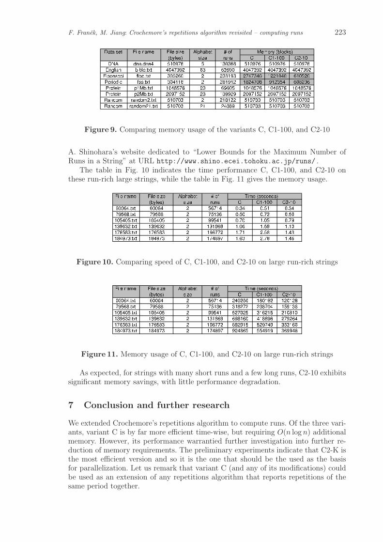
F. Franek, M. Jiang: Crochemore’s repetitions algorithm revisited – computing runs 223
Figure 9. Comparing memory usage of the variants C, C1-100, and C2-10
A. Shinohara’s website dedicated to “Lower Bounds for the Maximum Number ofRuns in a String” at URL http://www.shino.ecei.tohoku.ac.jp/runs/ .
The table in Fig. 10 indicates the time performance C, C1-100, and C2-10 onthese run-rich large strings, while the table in Fig. 11 gives the memory usage.
Figure 10. Comparing speed of C, C1-100, and C2-10 on large run-rich strings
Figure 11. Memory usage of C, C1-100, and C2-10 on large run-rich strings
As expected, for strings with many short runs and a few long runs, C2-10 exhibitssignificant memory savings, with little performance degradation.
7 Conclusion and further research
We extended Crochemore’s repetitions algorithm to compute runs. Of the three vari-ants, variant C is by far more efficient time-wise, but requiring O(n log n) additionalmemory. However, its performance warrantied further investigation into further re-duction of memory requirements. The preliminary experiments indicate that C2-K isthe most efficient version and so it is the one that should be the used as the basisfor parallelization. Let us remark that variant C (and any of its modifications) couldbe used as an extension of any repetitions algorithm that reports repetitions of thesame period together.

224 Proceedings of the Prague Stringology Conference 2009
References
1. M.I. Abouelhoda, S. Kurtz, and E. Ohlebusch: Replacing suffix trees with enhanced suffixarrays, J. Discr. Algorithms 2 (2004), pp. 53–86
2. G. Chen, S.J. Puglisi, and W.F. Smyth: Fast & practical algorithms for computing all theruns in a string, Proc. 18th Annual Symposium on Combinatorial Pattern Matching (2007),pp. 307–315
3. M. Crochemore: An optimal algorithm for computing the repetitions in a word, Inform.Process. Lett. 5 (5) 1981, pp. 297–315
4. M. Crochemore, C. Hancart, and T. Lecroq: Algorithms on Strings, Cambridge Univer-sity Press 2007
5. M. Crochemore and L. Ilie: Maximal repetitions in strings, Journal of Computer andSystem Sciences 74-5 (2008), pp. 796–807
6. M. Farach: Optimal suffix tree construction with large alphabets, 38th IEEE Symp. Found.Computer Science (1997), pp. 137–143
7. F. Franek, W.F. Smyth, and X. Xiao: A note on Crochemore’s repetitions algorithm, afast space-efficient approach, Nordic J. Computing 10-1 (2003), pp. 21–28
8. C. Iliopoulos, D. Moore, and W.F. Smyth: A characterization of the squares in a Fibonaccistring, Theoret. Comput. Sci.,172 (1997), pp. 281-291
9. R. Kolpakov and G. Kucherov: On maximal repetitions in words, J. of Discrete Algorithms,(1) 2000, pp. 159–186
10. J. Karkkainen and P. Sanders: Simple linear work suffix array construction, Proc. 30thInternat. Colloq. Automata, Languages & Programming (2003), pp. 943–955
11. P. Ko and S. Aluru: Space efficient linear time construction of suffix arrays, Proc. 14thAnnual Symp. Combinatorial Pattern Matching, R. Baeza-Yates, E. Chavez, and M. Crochemore(eds.), LNCS 2676, Springer-Verlag (2003), pp. 200–210
12. M.G. Main: Detecting leftmost maximal periodicities, Discrete Applied Math., (25) 1989,pp. 145–153
13. U. Manber and G. Myers: Suffix arrays: A new method for on-line string searches, SIAMJ. Comput. 22 (1993), pp. 935–938
14. P. Weiner: Linear pattern matching algorithms, Proc. 14th Annual IEEE Symp. Switching &Automata Theory (1973), pp. 1–11

Reducing Repetitions
Peter Leupold⋆
Department of Mathematics, Faculty of ScienceKyoto Sangyo UniversityKyoto 603-8555, Japan
Abstract. For a given word w, all the square-free words that can be reached by suc-cessive application of rewriting rules uu→ u constitute w’s duplication root. One wordcan have several such roots. We provide upper and lower bounds on the maximal num-ber of duplication roots of words of length n that show that this number is at leastexponential in n.
Keywords: repetitions in strings, DNA operations, duplication
1 Repetitions and Duplication
A mutation,.
which occurs frequently in DNA strands, is the duplication of a factorinside a strand [19]. The result is called a tandem repeat, and the detection of theserepeats has received a great deal of attention in bioinformatics [1,20]. The recon-struction of possible duplication histories of a gene is used in the investigation of theevolution of a species [24]. Thus duplicating factors and deleting halves of squaresis an interesting algorithmic problem with some motivation from bioinformatics, al-though squares do not need to be exact there. A very similar reduction was alsointroduced in the context of data compression by Ilie et al. [10,11]. They, howeverconserve information about each reduction step in the resulting string such that theoperation can also be undone again. In this way the original word can always be re-constructed, which is essential for data compression. We will present their approachin more detail in Section 3 and establish some relations between the two reductions.
So far, the interpretation of duplication as an operation on a string has mainlyinspired work in Formal Languages, most prominently the duplication closure. Dassowet al. introduced the duplication closure of a word and showed that the languagesgenerated are always regular over two letters [7]. Wang then proved that this is notthe case over three or more letters [23]. These results had actually been discoveredbefore in the context of copy systems [8], [3]. It remains an open problem, whethersuch duplication closures are always context-free or not. Later on, length boundsfor the duplicated factor were introduced [17], [15], and also the closure of languageclasses under the duplication operations was investigated [12]. Finally, also a specialtype of codes robust against duplications was investigated [16].
Besides considering duplication as a generative operation elongating strings, alsothe effects of the inverse operation on words have been the object of investigations[15]. Here duplications are undone, i.e. one half of them is deleted leaving behindonly the other half of the square. In this way words are reduced to square-free words,which are in some sense primitive under this notion; this is why we call the set of all
⋆ This work was done while Peter Leupold was funded as a post-doctoral fellow by the JapaneseSociety for the Promotion of Science under grant number P07810.
Peter Leupold: Reducing Repetitions, pp. 225–236.
Proceedings of PSC 2009, Jan Holub and Jan Zd’arek (Eds.), ISBN 978-80-01-04403-2 c© Czech Technical University in Prague, Czech Republic

226 Proceedings of the Prague Stringology Conference 2009
square-free words reachable from a given word w the duplication root of w in analogyto concepts like the primitive root or the periodicity root of words. Duplication rootsof languages were studied already in earlier work by the present author [14].
Here we will focus on duplication roots of single words. Mainly the followingquestion is addressed: how many different duplication roots can a word have? Weestablish an exponential lower bound for this number as well as an upper bound.Besides any possible applications, this study of how repetitions in a sequence can benested follows important lines of study in Combinatorics of Words, where repetitionshave been in the center of attention from the very start in the work of Thue [22].
2 Definitions
We assume the reader to be familiar with fundamental concepts from Formal Lan-guage Theory such as alphabet, word, and language, which can be found in manystandard textbooks like the one by Harrison [9]. The length of a finite word w isthe number of not necessarily distinct symbols it consists of and is written |w|. Thenumber of occurrences of a certain letter a in w is |w|a. The i-th symbol we denoteby w[i]. The notation w[i . . . j] is used to refer to the part of a word starting at thei-th position and ending at the j-th position.
A word u is a prefix of w if there exists an i ≤ |w| such that u = w[1 . . . i]; ifi < |w|, then the prefix is called proper. The set of all prefixes is pref(w). Suffixesare the corresponding concept reading from the back of the word to the front andthey are denoted by suff. We define the letter sequence seq(u) of a word u as follows:any word u can be uniquely factorized as u = xi1
1 xi22 · · ·xiℓ
ℓ for some integers ℓ ≥ 0and i1, i2, . . . , iℓ ≥ 1 and for letters x1, x2, . . . , xℓ such that always xj 6= xj+1; thenseq(u) := x1x2 · · ·xℓ. Intuitively speaking, every block of several adjacent occurrencesof the same letter is reduced to just one occurrence.
We call a word w square-free iff it does not contain any non-empty factor of theform u2, where exponents of words refer to iterated catenation, and thus ui is thei-fold catenation of the word u with itself. A word w has a positive integer k as aperiod, if for all i, j such that i ≡ j(modk) we have w[i] = w[j], if both w[i] and w[j]are defined.
For applying duplications to words we use string-rewriting systems. In our nota-tion we mostly follow Book and Otto [2] and define such a string-rewriting system Ron Σ to be a subset of Σ∗×Σ∗. Its single-step reduction relation is defined as u→R viff there exists (ℓ, r) ∈ R such that for some u1, u2 we have u = u1ℓu2 and v = u1ru2.We also write simpler just →, if it is clear which is the underlying rewriting system.
By∗→ we denote the relation’s reflexive and transitive closure, which is called the
reduction relation or rewrite relation. The inverse of a single-step reduction relation→ is →−1:= (r, ℓ) : (ℓ, r) ∈ R. Further notation that will be used is IRR(R) forthe set of words irreducible for a string-rewriting system R. With this we come to thedefinition of duplications.
The string-rewriting system we use here is the duplication relation defined asu♥v :⇔ ∃z[z ∈ Σ+ ∧ u = u1zu2 ∧ v = u1zzu2]. Notice how the symbol ♥ nicelyvisualizes the operation going from one origin to two equal halves. If we have lengthbounds |z| ≤ k or |z| = k on the factors to be duplicated we write ♥≤k or ♥krespectively; the relations are called bounded and uniformly bounded duplication re-spectively.

Peter Leupold: Reducing Repetitions 227
♥∗ is the reflexive and transitive closure of the relation ♥. The duplication closureof a word w is then w♥ := u : w♥∗u. The languages w♥≤k and w♥k are definedanalogously. Because our main topic is the reduction of squares, we will mainly usethe inverse of ♥ and will denote it by
.
:= ♥−1; the notations for length-boundedversions and iterated applications are used accordingly. Notice that for
. ≤k the lengthbound does not refer to the length of the rules’ left sides, but rather to half that length.This makes sense, because otherwise for all even k we would have
. ≤k =. ≤k+1,
and because this way the relations. ≤k and ♥≤k correspond. We will use a similar
convention when talking about squares. Thus we will say that a square u2 is of length|u|; in this case u will be called the base of this square.
With this we have all the prerequisites for defining the central notion of this work,the duplication root.
Definition 1. The duplication root of a non-empty word w is
♥√
w := IRR(.
) ∩ u : w.
∗ u.
As usual, this notion is extended in the canonical way from words to languages suchthat
♥√
L :=⋃
w∈L
♥√
w.
The roots ♥≤k√
w and ♥k√
w are defined in completely analogous ways, and also theseare extended to entire languages in the canonical way. When we want to contrast theduplication (root) without length bound to the bounded variants we will at times callit general duplication (root).
When talking about the elements of a word’s duplication root, we will also callthem simply roots; no confusion should arise. Similarly, where we say “the num-ber of roots” we mean the root’s cardinality. Though not completely correct, theseformulations are more compact and in many cases easier to understand.
Finally, notice that all words in a duplication root are square-free, and over analphabet of two letters only the seven square-free words λ, a, b, ab, ba, aba, bab exist.They are uniquely determined by their first letter, the last letter, and the set of lettersoccurring in them. Thus most problems about duplication roots are trivial unless wehave at least three letters. Therefore, unless otherwise stated, we will suppose analphabet of size at least three in what follows. First off, we illustrate this definitionwith an example that also shows that duplication roots are in general not unique,i.e., the set ♥
√w can contain more than one element as we will see further on.
Example 2. By undoing duplications, i.e., by applying rules from.
, we obtain fromthe word w = abcbabcbc the words in the set abc, abcbc, abcbabc ; in a first step eitherthe prefix (abcb)2 or the suffix (bc)2 can be reduced, only the former case results in aword with another square, which can be reduced to abc.
Thus we have the root ♥√
abcbabcbc = abc, abcbabc. Exhaustive search of allshorter words shows that this is a shortest possible example of a word with morethan one root over three letters.
Other examples with cardinalities of the root greater than two are the wordsw3 = babacabacbcabacb where
♥√
w3 = bacabacb, bacbcabacb, bacb,

228 Proceedings of the Prague Stringology Conference 2009
and w5 = ababcbabcacbabcabacbabcab where
♥√
w5 = abcbabcabacbabcab, abcbabcab, abcacbabcab, abcabacbabcab, abcab,
As the examples have finite length, the bounded duplication root is in generalnot unique either. The uniformly bounded duplication root, however, is known to beunique over any alphabet [15].
As already stated in the Introduction, so far research on duplication has mainlyfocused on its language theoretic properties. We recall the most important results onthese from [14].
Theorem 3. The closure properties of the classes of regular and context-free lan-guages under the three duplication roots are as follows:
♥k√
L ♥≤k√
L ♥√
L
REG Y Y NCF ? ? N
The symbol Y stands for closure, N stands for non-closure, and ? means that theproblem is open.
Here our focus is different. We will look in more detail at the duplication roots ofsingle words. One interesting question is how ambiguous it can be in relation to aword’s length.
Before we take a closer look at this question, however, we will now recall a notionthat is very closely related to our reduction.
3 The Relation to Repetition Complexity
In an effort to define a new measure for the complexity of words, Ilie et al. [10,11]defined a reduction relation very similar to undoing duplications, which however re-members the steps it takes, and in this way the original word can be restored fromthe reduced one. For the definition let D = 0, 1, . . . 9 be the set of decimal digits,and Σ be an alphabet disjoint from D. The alphabet for the reduction relation isT := Σ ∪ D ∪ 〈, 〉, ^. For a positive integer n let dec n denote its decimal rep-resentation. Then the reduction relation ⇒ is defined by u ⇒ v iff u = u1x
nu2,v = u1 〈x〉 ^〈dec n〉u2 for some u1, u2 ∈ T ∗, x = Σ+, n > 2. Finally, let h be themorphism erasing all symbols except the letters from Σ.
We illustrate in a simple example the different way of operation of the two rela-tions.
Example 4. For the word ababcbc there are two irreducible forms under ⇒, namely
〈ab〉〈2〉 cbc and aba 〈bc〉〈2〉. Under.
, however, the images of both words under hare further reducible to a common normal form: both ababcbc
.
abcbc.
abc andababcbc
.
ababc.
abc are possible reductions leading to abc. Notice how the brack-ets block the further reduction of abab in aba 〈bc〉 ^〈2〉 and of bcbc in 〈ab〉 ^〈2〉cbc.
There are two main differences between the two relations.
1. A reduction un ⇒ 〈u〉 ^〈n〉 is done in a single step while the reduction un.
∗ uwill always take n− 1 steps.

Peter Leupold: Reducing Repetitions 229
2. If w ⇒∗ u then w.
∗ h(u), but the reverse does not hold, see Example 4.
Despite these differences, the similarities are evident, and ⇒∗ can be embedded in.
∗ . We state a further relation.
Proposition 5. For a word w, if ♥√
w ⊆ h(u) : w ⇒∗ u then | ♥√w| = 1.
Proof. Let p and q be two different words in ♥√
w. Then there exist words u, p′, q′ suchthat w
.
∗ u, u.
p′.
∗ p, u.
q′.
∗ q, but no reductions p′.
∗ q or q′.
∗ p exist.Intuitively this means that the paths to p and q divide in the point u, which thus isa greatest lower bound of p, q in the set w . with
.
∗ as partial order. The twounduplications in u
.
p′ and u.
q′ must overlap, otherwise there would be a wordv such that p′
.
v and q′.
v. Let the two factors that are reduced be u2p and u2
q,where |up| > |uq| without loss of generality; notice that |up| = |uq| would result inp′ = q′.
The overlap of the unduplications must be greater than |uq|. Otherwise there is aw′ such that the unduplications are applied to a factor upw
′uq or uqw′up and the effect
can be seen as the deletion of up and uq; both would be possible consecutively. Further,the maximal repetition of up were it is reduced must be less than u3
p, otherwise thefactor uq would still be present after deletion of one up. This means that a reductionunder⇒ can only result in 〈up〉 ^〈2〉, no higher exponent, and no factor up can followon either side.
There can be no factor u2q directly preceding or following 〈up〉 on the side of the
overlap. Otherwise, again derivations p′.
v and q′.
v would have been possible.This means that the square u2
q in h(p′) cannot be reduced, neither can an equivalentreduction leading to the same result be done. Analogous reasoning holds for the casethat first u2
q is reduced to 〈uq〉 ^〈2〉, and thus h(u) : w ⇒∗ u cannot contain anysquare-free word.
⊓⊔
Intuitively this means that if ⇒ can reduce a word to a square-free one, then theoverlaps of its repetitive factors must be so minor that they do not lead to ambiguousduplication roots either. Already Example 4 shows that the converse of Proposition5 does not hold.
From the proof of Proposition 5 we can extract an important property of therelation
.
∗ that characterizes the situation, when two strings derived from thesame word can become incomparable.
Definition 6. Let w be a word. We will call two squares p2 and q2 a pair of criticalsquares in w, if w has a factor u such that
1. p2 ∈ pref(u),2. q2 ∈ suff(u),3. |u| ≤ 2(max(|p|, |q|)) + min(|p|, |q|)− 1.
Without further proof we state the following.
Lemma 7. Let w, p, and q be words such that w.
p and w.
q.If v : p
.
∗ v ∩ v : q.
∗ v = ∅, then w contains a pair of critical squares.

230 Proceedings of the Prague Stringology Conference 2009
4 The Number of Duplication Roots
A decisive question for any algorithmic problem related to duplication is the oneabout the possible number of duplication roots of a word with respect to its length.To find an exact bound seems to be a very intricate problem, and so we try to findgood upper and lower bounds on this number. More formally, we try to find boundsfor the function defined as
duproots(n) := max| ♥√w| : |w| = n.The function duproots is monotonically growing. For any word w, duplicate one of itsletters to obtain a word w′ of length |w| + 1. Clearly w′
.
w and thus ♥√
w ⊆ ♥√
w′.Consequently we have duproots(n) ≤ duproots(n + 1) for all n > 0. Therefore writing|w| = n in the definition is equivalent to writing |w| ≤ n.
Because it has often turned out to be very useful to consider problems aboutduplications with a length restriction, we also define the function
bduproots≤ k(n) := max| ♥≤k√
w| : |w| = n.
By definition we have bduproots≤k ≤ duproots and bduproots≤k ≤ bduproots≤k+1 forall k > 0. We now try to characterize the growth of the function duproots moreexactly.
4.1 Bounding from Above
Obviously, rules from.
can only be applied on square factors. Thus the number ofsquares is the number of possible distinct rule applications in a string. However, whenwe are interested in rule applications with distinct result and thus with potentiallydistinct roots, the number of runs captures this more exactly.
Recall that a run is a maximal repetition of exponent at least two in a string. Itis known that the number of runs in a string of length n is linearly bounded by n[13]. A great deal of work has been done to determine the constant c such that c · nis the exact bound. The most recent results indicate that c lies between 1.6 [6] and0.94 [18]. The following fact shows how this number plays a role for the number ofpossible reductions via
.
and thus for the number of duplication roots.
Fact 8. Let w be a word with period k. Then all applications of rules from. k will
result in the same word, i.e. u : w. k u is a singleton set.
As a consequence of this, the number of distinct descendants of w with respect to.
is equal to the number of runs in w. In this way. the number of runs seems to playan important role for the computation of the maximal number of duplication roots.
To obtain a first approximation on this number, let us state the following: thenumber of runs in a string of length n is bounded linearly by the string’s length.Reducing one square leaves the word’s length in general in the order of n, thus alsothe number of runs is again in the order of n.
On the other hand, every reduction via.
removes at least one letter, thus therecan be at most n − 1 steps in the reduction of a word of length n. More precisely,observe that deleting one half of a square cannot remove all copies of a letter froma given string. Thus all roots of a word over three letters have at least three lettersthemselves. Overall, there are up to n− 3 times up to n choices for reducing squares,

Peter Leupold: Reducing Repetitions 231
and the number of different reduction paths lies in O(nn). Using the upper bound onthe number of runs we see that
duproots(n) ≤ (1.6n)n−3.
Of course, this gives a very rough upper bound. Most importantly, it disregards thefact that many reductions starting in different points will converge again at somepoint. Obviously, two rule applications in factors that do not overlap can be appliedin either order with identical result. Further, not all of the strings reachable during areduction will reach the maximum number of runs.
We recall a result from [14].
Lemma 9. If for two words u, v ∈ Σ∗ we have seq(u) = seq(v), then also ♥√
u =♥√
v = ♥√
seq(u).
This means that we can first do all the possible reductions of the form x2 → x forsingle letters x. So for possible splits to different duplication roots we can assumethat at least two letters are deleted in every step. Actually, also the fact that u fromExample 4 is the shortest possible word with at least two distinct duplication rootsshows that we need only consider applications of rules u2 → u with |u| ≥ 2. This
lowers our upper bound to (1.6n)n−3
2 .The improvement is not substantial, however. In the initial approach, in some
sense all possible paths from w to words in ♥√
w in the Hasse diagram of the partial
order [w . ,.
∗] are counted. The improved version counts only the paths startingfrom seq(w) as depicted in Figure 1. The optimal case, however would be to countonly one path per element of ♥
√w. We can take another step into this direction for
the partial order [w .
≤k,. ≤k
∗]. As exemplary value for k we choose 30, the reasonfor this will become evident in the next section.
Figure 1. 10 versus 2 paths for the word aabcbabcbbc, by first reducing one-lettersquares from left to right. The direction of reductions is top to bottom.
Lemma 7 characterizes the words, from which it may not be possible to rejoinoutgoing paths. They need to have a critical overlap. The involved squares’ basescannot be longer than 30. Further, one must be shorter than the other, but of length atleast two. So for a given square, there are at most 29 such candidates. They can overlapon either side, which gives 56 possible combinations. The shorter square must havemore than one half of its length inside the other, and at least one letter must be outside

232 Proceedings of the Prague Stringology Conference 2009
the other. So for a square of length m we have m− 1 possible positions. The overallnumber of possible configurations is therefore 2
∑2≤i≤29 i− 1 = 2
∑1≤i≤28 i = 812.
For calculating the number of possible roots of a word w, we now employ thefollowing tactics. Again, we first compute seq(w). Then we do not follow all possiblepaths from seq(w), but rather select one random square. If it does not form partof a pair of critical squares, then we simply reduce it and proceed further with thenext square. Otherwise, for all critical pairs we follow also the paths resulting fromreducing the possible partners in these pairs. As we have seen, a square of length 30can form part of at most 812 critical pairs. The length of the paths is subject to thesame bound as for
.
, and thus we have to follow at most 812n−3
2 paths, which isthe upper bound on bduproots≤30.
Clearly, especially the first bound of (1.6n)n−3
2 is very far off the real value. Indeed,all roots of a word w are shorter than w unless w is square-free. Let us label w’s lettersfrom the start to the end. We can look at a rule uu→ u like the deletion of one copyof u, so its labels disappear. Thus every word in ♥
√w corresponds to a subset of the
set of |w| labels. There are only 2|w| such subsets, which gives us a much better upperbound, also independent of the alphabet size. We still have given the construction ofour bound, because we feel that it bears potential for improvement even beyond 2|w|.Intuitively, the linear bound on the number of runs in a string means that they mustbe distributed rather evenly over the string’s length. Further, results like the Theoremof Fine and Wilf suggest that one run can only form a very limited number of pairs ofcritical squares, so that even in the case of unbounded duplication we should be ableto get an average constant bound like the one of 812 for
. ≤30. By careful analysis ofthe possibilities, it should be possible to lower the bound even beyond 2|w|.
4.2 Bounding from Below
The upper bound on the number of duplication roots is very high and raises thequestion how far from the real number it is. By an example we now establish a lowerbound for this number, which is also exponential. Thus it shows that the upper boundis not too bad.
Example 10. We construct an example of a sequence of words wn, which are simplypowers of a word w, namely wn := wn. The number of roots increases exponentially inn. This is a modification of a construction used earlier to present a simple languagewith infinite duplication root [14]. We start the construction of w from the wordu = abcbabcbc; in Example 2 we have seen that the root of u consists of the two wordsu1 = abc and u2 = abcbabc. The basic idea is to concatenate copies of u; in everyfactor there is the choice of u1 or u2 and thus every additional copy of u doubles thenumber of roots. However, simple concatenation of u would allow further reductions.Therefore we need to modify and separate the different copies of u in ways thatprevent the creation of further squares.
The first measure we take is permuting the letters. Let ρ be the morphism, whichsimply renames letters according to the scheme a → b → c → a. Then ρ(u) has thetwo roots ρ(u1) and ρ(u2); similarly, ρ(ρ(u)) has the two roots ρ(ρ(u1)) and ρ(ρ(u2)).
We will now use this ambiguity to construct the word w. This word over thefour-letter alphabet a, b, c, d is
w = udρ(u)dρ(ρ(u))d = abcbabcbc · d · bcacbcaca · d · cabacabab · d.

Peter Leupold: Reducing Repetitions 233
Thus the duplication root of w contains among others the three words
wa = abc · d · bca · d · cabacab · dwb = abc · d · bcacbca · d · cab · dwc = abcbabc · d · bca · d · cab · d,
which are square-free. We now need to recall that a morphism h is called square-free, iff h(v) is square-free for all square-free words v. Crochemore has shown thata uniform morphism h is square-free iff it is square-free for all square-free words oflength 3 [5]. Here uniform means that all images of single letters have the same length,which is given in our case.
The morphism we define now is ϕ(x) := wx for all x ∈ a, b, c. Thus to establishthe square-freeness of ϕ, we need to check this property for the images of all square-free words up to length 3. These are
ϕ(aba) = abcdbcadcabacabdabcdbcacbcadcabdabcdbcadcabacabdϕ(abc) = abcdbcadcabacabdabcdbcacbcadcabdabcbabcdbcadcabdϕ(aca) = abcdbcadcabacabdabcbabcdbcadcabdabcdbcadcabacabdϕ(acb) = abcdbcadcabacabdabcbabcdbcadcabdabcdbcacbcadcabdϕ(bab) = abcdbcacbcadcabdabcdbcadcabacabdabcdbcacbcadcabdϕ(bac) = abcdbcacbcadcabdabcdbcadcabacabdabcbabcdbcadcabdϕ(bca) = abcdbcacbcadcabdabcbabcdbcadcabdabcdbcadcabacabdϕ(bcb) = abcdbcacbcadcabdabcbabcdbcadcabdabcdbcacbcadcabdϕ(cac) = abcbabcdbcadcabdabcdbcadcabacabdabcbabcdbcadcabdϕ(cab) = abcbabcdbcadcabdabcdbcadcabacabdabcdbcacbcadcabdϕ(cba) = abcbabcdbcadcabdabcdbcacbcadcabdabcdbcadcabacabdϕ(cbc) = abcbabcdbcadcabdabcdbcacbcadcabdabcbabcdbcadcabd,
where, of course, the images of all words shorter than three are contained in them.All the twelve words listed here are indeed square-free as an eager reader can check,and thus ϕ is square-free.
Now let t be an infinite square-free word over the letters a, b and c. Such a wordexists [22]. Then all the words in ϕ(pref(t)) are square-free, too. From the constructionof ϕ we know that for any word z of length i we can reach ϕ(z) from wi by undoing
duplications. Therefore ϕ(pref(t)) ⊆ ♥√
w+. For two distinct square-free words t1 andt2, also ϕ(t1) 6= ϕ(t2). Finally, notice that for all positive i ≤ n we have wn
.
∗ wi.This means that all square-free words that are not longer than n lead to a different
duplication root of wn. Therefore bduproots≤30 ≤ s, where s(n) is the number ofternary square-free words of length up to n. This function’s value is not known,however, it was first bounded to 6 · 1.032n ≤ s(n) ≤ 6 · 1.379n by Brandenburg[4]. A better lower bound was found by Sun s(n) ≥ 110
n42 [21]. w itself is of length
3|u|+ 3 = 30. So we see that bduproots≤30(n) ≥ 130
110n42 .
Example 10 leaves room for improvement in several respects.
– The word w is over a four-letter alphabet. The letter d is used to separate thedifferent blocks that introduce the ambiguities and only use the alphabet a, b, c.The question is whether this function can also be fulfilled by an appropriate wordover a, b, c; computer experiments with candidate words have always led tounwanted squares with some of the adjoining factors.

234 Proceedings of the Prague Stringology Conference 2009
– The ambiguity of u that we use is only two-fold. Using the words w3 and w5 fromExample 2, it might be possible to pack more choices into less room and thusimprove the initial constant of 1
5with similar constructions. However, this would
not change the magnitude. On the other hand, the resulting morphism would notbe uniform, which would complicate the establishment of its square-freeness.
Summarizing this section up to this point, we have the following bounds for thefunction duproots.
Proposition 11. 130
110n42 ≤ duproots(n) ≤ 2n for all n > 0.
Because Example 10 uses only rules from. ≤30, its bound holds also for bduproots≤30.
So for this function we get a much sharper characterization of its growth.
Proposition 12. 130
110n42 ≤ bduproots≤30(n) ≤ max812
n−32 , 2n for all n > 0.
While this upper bound is still enormous, we have at least achieved a bounding be-tween two exponential functions. So for this case the bounds are much tighter, thoughstill rather loose. For ternary alphabet, the upper bound 6 · 1.379n by Brandenburgcan replace 2n in both Propositions.
4.3 Computing the Number of Duplication Roots
Proposition 11 shows that the straight-forward approach to computing the functionduproots will lead to exponential runtime. But it seems reasonable to assume thatit is not necessary to actually compute the set ♥
√w to determine its size. Example
4 suggests that it suffices to identify the number of critical overlaps in the originalword. In this case, even linear time might suffice. However, it remains to show thatno new critical pairs can come up during a reduction, or at least that their numbercan be foreseen by looking a the original word.
5 Open Problems
The first and most evident problem is, of course, a better characterization of thefunction duproots. We conjecture that in some way a bounding will be possible in away similar to that for bduproots, and thus also duproots can be bounded from aboveand below by exponential functions. For this a refined analysis of pairs of criticalsquares might be the key, just as for a linear time algorithm to actually computeduproots.
Besides this, three more algorithmic problems related to the duplication root of aword suggest themselves.
(i) Duplication Root: For a given word w, find one of its duplication roots.(ii) Minimal Duplication Root: For a given word w, find one of the shortest of
its duplication roots.(iii) Complete Duplication Root: For a given word w, find all of its duplication
roots.
To solve Problem (i) we can follow any reduction. As seen above, these can take up ton steps. In each step one square must be detected and reduced. Therefore a runtimeof O(n2 log n) can be expected. An interesting question is whether Problem (ii) can

Peter Leupold: Reducing Repetitions 235
be solved faster than Problem (iii), i.e. do we basically have to enumerate the entireroot to know which is its smallest element, or can, for example, a greedy strategyeliminate many candidate reductions early on. No exact results on the complexity ofany of the three problems are known.
Another interesting field is finding restrictions on the general duplication whichare on the one hand motivated from practical considerations like possible tandemrepeats in DNA, and on the other hand make the problems described here moretractable. Since tandem repeats cannot occur at arbitrary factors of a DNA strand,there might be less than exponentially many possible duplication histories for DNAstrands.
Acknowledgments. The words w3 and w5 from Example 2 were found by Szilard ZsoltFazekas, the fact that w is the shortest example of a word with ambiguous root wasestablished by Artiom Alhazov with a computer. The observation that the numberof subsets of a set with |w| elements bounds | ♥√w| was first made by Masami Ito.
References
1. D. A. Benson: Tandem repeat finder: A program to analyze DNA sequences. Nucleic AcidsResearch, 27(2) 1999, pp. 573–580.
2. R. Book and F. Otto: String-Rewriting Systems, Springer, Berlin, 1993.3. D. P. Bovet and S. Varricchio: On the regularity of languages on a binary alphabet generated
by copying systems. Information Processing Letters, 44(3) 1992, pp. 119–123.4. F.-J. Brandenburg: Uniformly growing k-th power-free homomorphisms. Theor. Comput.
Sci., 23 1983, pp. 69–82.5. M. Crochemore: Sharp characterizations of squarefree morphisms. Theoretical Computer
Science, 18 1982, pp. 221–226.6. M. Crochemore and L. Ilie: Maximal repetitions in strings. Journal of Computer and
System Sciences, 74(5) 2008, pp. 796–807.7. J. Dassow, V. Mitrana, and G. Paun: On the regularity of duplication closure. Bulletin of
the EATCS, 69 1999, pp. 133–136.8. A. Ehrenfeucht and G. Rozenberg: On the separating power of EOL systems. RAIRO
Informatique Thorique, 17(1) 1983, pp. 13–22.9. M. A. Harrison: Introduction to Formal Language Theory, Addison-Wesley, Reading, Mas-
sachusetts, 1978.10. L. Ilie, S. Yu, and K. Zhang: Repetition complexity of words, in COCOON, O. H. Ibarra and
L. Zhang, eds., vol. 2387 of Lecture Notes in Computer Science, Springer, 2002, pp. 320–329.11. L. Ilie, S. Yu, and K. Zhang: Word complexity and repetitions in words. Int. J. Found.
Comput. Sci., 15(1) 2004, pp. 41–55.12. M. Ito, P. Leupold, and K. Shikishima-Tsuji: Closure of language classes under bounded
duplication, in Developments in Language Theory, O. H. Ibarra and Z. Dang, eds., vol. 4036 ofLecture Notes in Computer Science, Springer, 2006, pp. 238–247.
13. R. M. Kolpakov and G. Kucherov: Finding maximal repetitions in a word in linear time,in FOCS, 1999, pp. 596–604.
14. P. Leupold: Duplication roots, in Developments in Language Theory, T. Harju, J. Karhumaki,and A. Lepisto, eds., vol. 4588 of Lecture Notes in Computer Science, Springer, 2007, pp. 290–299.
15. P. Leupold, C. Martın-Vide, and V. Mitrana: Uniformly bounded duplication languages.Discrete Applied Mathematics, 146(3) 2005, pp. 301–310.
16. P. Leupold and V. Mitrana: Uniformly bounded duplication codes. Theor. Inform. Appl.,41(4) 2007, pp. 411–424.
17. P. Leupold, V. Mitrana, and J. M. Sempere: Formal languages arising from gene repeatedduplication, in Aspects of Molecular Computing, N. Jonoska, G. Paun, and G. Rozenberg, eds.,vol. 2950 of Lecture Notes in Computer Science, Springer, 2004, pp. 297–308.

236 Proceedings of the Prague Stringology Conference 2009
18. W. Matsubara, K. Kusano, A. Ishino, H. Bannai, and A. Shinohara: New lowerbounds for the maximum number of runs in a string, in Proceedings of the Prague StringologyConference 2008, J. Holub and J. Zdarek, eds., Czech Technical University in Prague, CzechRepublic, 2008, pp. 140–145.
19. E. Pennisi: MOLECULAR EVOLUTION: Genome Duplications: The Stuff of Evolution? Sci-ence, 294(5551) 2001, pp. 2458–2460.
20. D. Sokol, G. Benson, and J. Tojeira: Tandem repeats over the edit distance. Bioinformatics,23(2) 2007, pp. 30–35.
21. X. Sun: New lower bound on the number of ternary square-free words. Journal of IntegerSequences, 6(3) 2003, pp. 1–8.
22. A. Thue: Uber die gegenseitige Lage gleicher Teile verschiedener Zeichenreihen. Norske Vi-denskabers Selskabs Skrifter Mat.-Nat. Kl. (Kristiania), 1 1912, pp. 1–67.
23. M.-W. Wang: On the irregularity of the duplication closure. Bull. EATCS, 70 2000, pp. 162–163.
24. I. Wapinski, A. Pfeffer, N. Friedman, and A. Regev: Natural history and evolutionaryprinciples of gene duplication in fungi. Nature, 449 2007, pp. 54–61.

Asymptotic Behaviour of the Maximal Number
of Squares in Standard Sturmian Words
(Extended Abstract)
Marcin Piatkowski2⋆ and Wojciech Rytter1,2⋆⋆
1 Department of Mathematics, Computer Science and Mechanics,University of Warsaw, Warsaw, Poland
[email protected] Faculty of Mathematics and Informatics,
Nicolaus Copernicus University, Torun, [email protected]
Abstract. Denote by sq(w) the number of distinct squares in a string w and let Sbe the class of standard Sturmian words. They are generalizations of Fibonacci wordsand are important in combinatorics on words. For Fibonacci words the asymptoticbehaviour of the number of runs and the number of squares is the same. We showthat for Sturmian words the situation is quite different. The tight bound 8
10 |w| for thenumber of runs was given in [3]. In this paper we show that the tight bound for themaximal number of squares is 9
10 |w|. We use the results of [11] where exact (but notclosed) complicated formulas were given for sq(w) for w ∈ S and we show:
(1) for all w ∈ S sq(w) ≤ 910 |w|+ 4,
(2) there is an infinite sequence of words wk ∈ S such that
limk→∞
|wk| = ∞ and limk→∞
sq(wk)
|wk|=
9
10.
Surprisingly the maximal number of runs is reached by the words with recurrences oflength only 5. This contrasts with the situation of Fibbonaci words, though standardSturmian words are natural extension of Fibonacci words. If this length drops to 4,the asymtotic behaviour of the maximal number of squares falls down significantlybelow 9
10 |w|. The structure of Sturmian words rich in squares has been discovered byus experimentally and verified theoretically. The upper bound is much harder, its proofis not a matter of simple calculations. The summation formulas for the number ofsquares are complicated, no closed formula is known. Some nontrivial reductions werenecessary.
1 Introduction
A square in a string is a subword of the form ww, where w is nonempty. The squaresare a simplest form of repetitions, despite the simple formulation many combinato-rial problems related to squares are not well understood. The subject of computingmaximal number of squares and repetitions in words is one of the fundamental topicsin combinatorics on words [18,22] initiated by A. Thue [28], as well as it is importantin other areas: lossless compression, word representation, computational biology, etc.
⋆ The research supported by Ministry of Science and Higher Education of Poland,grant N N206 258035.
⋆⋆ Supported by grant N206 004 32/0806 of the Polish Ministry of Science and Higher Education.
Marcin Piatkowski, Wojciech Rytter : Asymptotic Behaviour of the Maximal Number of Squares in Standard Sturmian Words, pp. 237–248.
Proceedings of PSC 2009, Jan Holub and Jan Zd’arek (Eds.), ISBN 978-80-01-04403-2 c© Czech Technical University in Prague, Czech Republic

238 Proceedings of the Prague Stringology Conference 2009
Let sq(w) be the number of distinct squares in the word w and sq(n) be themaximal number of distinct squares in the word of length n. The behaviour of thefunction sq(n) is not well understood, though the subject of squares was studied bymany authors, see [9,10,17]. The best known results related to the value of sq(n) are,see [13,15,16]:
n− o(n) ≤ sq(n) ≤ 2n−O(log n).
In this paper we concentrate on the asymptotic behaviour of the maximal number ofsquares in class of standard Sturmian words S. We show: for all w ∈ S sq(w) ≤ 9
10|w|
and there is an infinite sequence of strictly growing words wk ∈ S such that
limk→∞
sq(wk)
|wk|=
9
10.
There are known efficient algorithms for the computation of integer powersin words, see [2,6,11,23,24]. The powers in words are related to maximal repeti-tions, also called runs. It is surprising that the known bounds for the number ofruns are much tighter than for squares, this is due to the work of many people[3,7,8,14,19,20,25,26,27].
One of interesting questions related to squares is the relation of their number tothe number of runs. In case of Fibonacci words the number of squares and runs differonly by 1.
The results of this paper show that the maximal number of squares and the max-imal number of runs are possibly not closely related, since in case of well structuredwords (Sturmian words) the density ratio of squares (the asymptotic quotient of themaximal number of squares by the size of the string) is 9
10and for runs it is 8
10.
2 Standard Sturmian words
The standard Sturmian words (standard words, in short) are generalization of Fi-bonacci words and have a very simple grammar-based representation which has somealgorithmic consequences.
Let S denote the set of all standard Sturmian words. These words are defined overa binary alphabet Σ = a, b and are described by recurrences (or grammar-basedrepresentation) corresponding to so called directive sequences: integer sequences
γ = (γ0, γ1, . . . , γn),
where γ0 ≥ 0, γi > 0 for 0 < i ≤ n.
The word xn+1 corresponding to γ, denoted by Sw(γ), is defined by recurrences:
x−1 = b, x0 = a,
x1 = xγ0
0 x−1, x2 = xγ1
1 x0,
. . . . . .
xn = xγn−1
n−1 xn−2, xn+1 = xγnn xn−1.
(1)
Fibonacci words are standard Sturmian words given by the directive sequencesof the form γ = (1, 1, . . . , 1) (n-th Fibonacci word Fn corresponds to a sequence of

M. Piatkowski, W. Rytter: Asymptotic Behaviour of the Maximal Number of Squares in. . . 239
n ones). We consider here standard words starting with the letter a, hence assumeγ0 > 0. The case γ0 = 0 can be considered similarly.
For even n > 0 a standard word xn has the suffix ba, and for odd n > 0 it has thesuffix ab. The number N = |xn+1| is the (real) size, while n+1 can be thought as thecompressed size.
Example 1.Consider directive sequence γ = (1, 2, 1, 3, 1). We have:
Sw(1, 2, 1, 3, 1) = ababaabababaabababaabababaababaab
x−1 = b, x0 = a, x1 = x10x−1 = a b, x2 = x2
1x0 = ab ab a,
x3 = x12x1 = ababa ab, x4 = x3
3x2 = ababaab ababaab ababaab ababa,
x5 = x14x3 = ababaabababaabababaabababa ababaab
The grammar-based compression consists in describing a given word by a context-free grammar G generating this (single) word. The size of the grammar G is thetotal length of all productions of G. In particular each directive sequence of a stan-dard Sturmian word corresponds to such a compression – the sequence of recurrencescorresponding to the directive sequence. In this case the size of the grammar is pro-portional to the length of the directive sequence.
For some lexicographic properties and structure of repetitions of standard Stur-mian words see [5,3,1,4].
3 Summation formulas for the number of squares
The exact formulas for the number of squares in standard Sturmian words were givenby Damanik and Lenz in [11]. In this section we reformulate their formulas to havecompact version more suitable for the asymptotic analysis. The formulas are rathercomplicated and such an analysis is nontrivial. It will be done in the section 5.
Denote qi = |xi|, where xi are as in equation (1). The following lemma charecterizethe possible lengths of periods of squares in Sturmian words.
Lemma 2. ([11])Let w = Sw(γ0, γ1, . . . , γn) be a standard Sturmian word. Each primitive period of asquare in w has the length kqi for 1 ≤ k ≤ γi or kqi + qi−1 for 1 ≤ k < γi.
The squares in standard Sturmian word w with period of the length kqi for 1 ≤k ≤ γi or kqi + qi−1 for 1 ≤ k < γi are said to be of type i.
Example 3.Consider the word from Example 1:
Sw(1, 2, 1, 3, 1) = ababaabababaabababaabababaababaab.
We have:
one square of type 0: a·a,
three squares of type 1 (period 2, 3): ab·ab, ba·ba, aba·aba,
three squares of type 2 (period 5): ababa·ababa, babaab·babaab, abaab·abaab,
and eleven squares of type 3 (with periods 7,14):

240 Proceedings of the Prague Stringology Conference 2009
ababaab·ababaab, babaaba·babaaba, abaabab·abaabab, baababa·baababa,
aababab·aababab, abababa·abababa, bababaa·bababaa,
ababaabababaab·ababaabababaab, babaabababaaba·babaabababaaba,
abaabababaabab·abaabababaabab, baabababaababa·baabababaababa.
Let sqi(γ0, γ1, . . . , γn), for 1 ≤ i ≤ n, be the number of squares of the type i andlet sq0(γ0, γ1, . . . , γn) be the number of squares with period of the form a+ in theword Sw(γ0, γ1, . . . , γn).
We slightly abuse the notation and denote sq(γ0, γ1, ..., γn) = sq(Sw(γ0, γ1, ..., γn)
).
Denote d(0) =⌊
γ0+12
⌋and for 1 ≤ i ≤ n and γ = (γ0, γ1, . . . , γn):
d1(i) =
γi
2qi + qi−1 − 1 for even γi
γi
2qi + 1
2qi for odd γi
d(i) = d1(i) + γi qi − qi − γi + 1.
Let Sw(γ0, γ1, . . . , γn) be a standard Sturmian word. Then sq(γ0, γ1, . . . , γn) isdetermined as follows, see [11]:
Summation formulas:
(1) sq(γ0, γ1, . . . , γn) =∑n
i=0 sqi(γ0, γ1, . . . , γn).
(2) (0 ≤ i ≤ n− 3) or (i = n− 2 & γn ≥ 2) ⇒ sqi(γ) = d(i).
(3) γn = 1 ⇒ sqn−2(γ) =
d(n− 2)− qn−3 + 1 for even γn−2
d(n− 2)− qn−2 + qn−3 + 1 otherwise
(4) γn = 1 ⇒ sqn−1(γ) =
d1(n− 1)− qn−2 + 1 for even γn−1
d1(n− 1)− qn−1 + qn−2 − 1 otherwise
(5) γn > 1 ⇒ sqn−1(γ) =
d(n− 1)− qn−2 + 1 for even γn−1
d(n− 1)− qn−1 + qn−2 − 1 otherwise
(6) sqn(γ) =
d1(n)− qn + 2 for even γn
d1(n)− qn otherwise

M. Piatkowski, W. Rytter: Asymptotic Behaviour of the Maximal Number of Squares in. . . 241
4 Sturmian words with many squares
In this section we present and analyse the sequence wk of Sturmian words achievingasymptotically maximal ratio:
limk→∞|wk| =∞ and lim
k→∞
squares(wk)
|wk|=
9
10.
Recall that the squares with periods kqi for 1 ≤ k ≤ γi or kqi + qi−1 are said tobe of the type i.
Consider the wordswk = Sw(k, k, 2, 1, 1).
Example 4.
w1 = Sw(1, 1, 2, 1, 1) = (aba)2ab(aba)3ab,
w2 = Sw(2, 2, 2, 1, 1) =((aab)2a
)2
aab((aab)2a
)3
aab,
w3 = Sw(3, 3, 2, 1, 1) =((aaab)3a
)2
aaab((aaab)3a
)3
aaab.
Sw(3, 3, 2, 1, 1) is illustrated in Figure 1.
a a a ba a a b a a a b a a a a ba a a b a a a b a a a a b a a a b a a a b a a a ba a a a b a a a ba a a ba a a a b a a a ba a a ba a a a b1 1 0
1 1 0
2
3
2
Figure 1. The squares in word Sw(3, 3, 2, 1, 1) with their shifts and types.
Theorem 5.We have sq(k, k, 2, 1, 1) −→ 9
10·∣∣∣Sw(γ0, γ1, . . . , γn)
∣∣∣ for k −→∞.
Proof.Let γ = (k, k, 2, 1, 1). We have:
Sw(γ) =((akb)ka
)2
akb((akb)ka
)3
akb
and|Sw(γ)| = 5k2 + 7k + 7.
We compute separately the number of squares for each type 0 ≤ i ≤ 4.
There are two cases depending on the parity of k and we can assume that k > 1.

242 Proceedings of the Prague Stringology Conference 2009
Case 1: k is odd.
We have (according to our formulas):
sq0(γ) =1
2
(k + 1
),
sq1(γ) =1
2
(3k2 + 1
),
sq2(γ) = 2k2 + 2k + 1,
sq3(γ) = k2 + k,
sq4(γ) = 0,
sq(γ) =1
2
(9k2 + 7k + 4
).
Finally
limk→∞
sq(γ)
|Sw(γ)| = limk→∞
9k2 + 7k + 4
10k2 + 14k + 14= 0.9 .
Case 2: k is even.
We have (according to our formulas):
sq0(γ) =1
2k,
sq1(γ) =1
2
(3k2 − k
),
sq2(γ) = 2k2 + 2k + 1,
sq3(γ) = k2 + k,
sq4(γ) = 0,
sq(γ) =1
2
(9k2 + 6k + 2
).
Finally
limk→∞
sq(γ)
|Sw(γ)| = limk→∞
9k2 + 6k + 2
10k2 + 14k + 14= 0.9.
This concludes the proof.
5 Asymptotic behaviour of the maximal number of squares
The formulas (1-6) from the section 3 give together the value of sq(γ), however thereis no close simple formula. Therefore tight asymptotic estimations are nontrivial. Westart with an estimation for short γ. The proof of the following simple lemma isomitted in this version.
Lemma 6. [Short γ]sq(γ0, γ1, γ2) ≤ 7
3|Sw(γ0, γ1, γ2)| and sq(γ0, γ1, γ2) ≤ |Sw(γ0, γ1, γ2)| − 4.

M. Piatkowski, W. Rytter: Asymptotic Behaviour of the Maximal Number of Squares in. . . 243
For a word w of length at least 2 denote by exch2(w) the word resulting from w byexchanging the last two letters.
Lemma 7. sq(w) ≤ sq(exch2(w)
)+ 4.
Proof.It is known, see [13], that there are at most two last occurrences of different squares ata single position in a string. If we reverse the word then this corresponds to the end-positions of the first occurrences. Hence at the last two positions at most 4 differentsquares can end which do not appear earlier in the same word with the last two lettersremoved. This completes the proof.
The next two lemmas allows us to restrict the values of last two elements of thedirective sequence in the asymptotic estimation of sq(γ).
Lemma 8. [Reduction of γn]Let Sw(γ0, γ1, . . . , γn) be a standard Sturmian word. If γn > 1 then
sq(γ0, . . . , γn−1, γn) ≤ sq(γ0, . . . , γn−1, γn − 1, 1) + 4.
Proof.The words Sw(γ0, . . . , γn− 1, 1) and Sw(γ0, . . . , γn) differ only on the last two letters,see [18]. Hence
Sw(γ0, . . . , γn − 1, 1) = exch2
(Sw(γ0, . . . , γn)
).
Now the thesis follows from the Lemma 7.
Lemma 9. [Reduction of γn−1]Let x = SW (γ0, . . . , γn−2, γn−1, 1), x′ = SW (γ0, . . . , γn−2, 1, 1),x′′ = SW (γ0, . . . , γn−2, 2, 1).Then (
sq(x′) ≤ 9
10|x′| and sq(x′′) <
9
10|x′′|
)⇒ sq(x) ≤ 9
10|x|.
Proof.If γn−1 is odd then let ∆ = γn−1 − 1 otherwise let ∆ = γn−1 − 2.Consider what happens when we change γn−2 by the quantity ∆.The increase of the number of squares is ∆
2qn−1, while the increase in the length of
the word is ∆ qn−1. The increase of squares is amortized by half of the increase of thelength. Therefore we can subtract ∆ from γn−1.
Observation
d(i) ≤
(3
2γi − 1
)qi + qi−1 − 1 for even γi
(3
2γi −
1
2
)qi for odd γi

244 Proceedings of the Prague Stringology Conference 2009
Lemma 10.For 2 ≤ r ≤ n− 3 we have
r∑
i=0
d(i) <3
2qr+1 + qr.
Proof.According to the observation above and implication
γi ≥ 2 ⇒ qi−1 − qi < − 1
2qi,
we have:
d(i) ≤ 3
2γi qi −
1
2qi.
Observe now that γi qi = qi+1 − qi−1. Hence for r ≥ 2:
r∑
i=1
γi qi = qr+1 + qr − q0 − q1.
Consequently
r∑
i=0
d(i) < d(0) +3
2
r∑
i=1
γi qi −1
2qr
≤ d(0) +3
2
(qr+1 + qr − q0 − q1
)− 1
2qr
≤ 3
2qr+1 + qr.
This completes the proof.
Now we are ready to prove the tight bound for the number of squares in standardSturmian words.
Theorem 11.Let Sw(γ0, γ1, . . . , γn) be a standard Sturmian word. Then
sq(γ0, γ1, . . . , γn) ≤ 9
10·∣∣∣Sw(γ0, γ1, . . . , γn)
∣∣∣ + 4.
Proof.First assume that:
γn = 1 and γn−1 ∈ 1, 2
Let us shorten the notation and denote:
A = qn−2, B = qn−3, α = γn−2.
We have, due to Lemma 10, the following fact (in terms of A and B):

M. Piatkowski, W. Rytter: Asymptotic Behaviour of the Maximal Number of Squares in. . . 245
Claim 1.n−3∑
i=0
sqi(γ) =n−3∑
i=0
d(i) ≤ 3
2A + B.
This, together with the fact that sqn(γ0, γ1, . . . , γn−1, 1) = 0, implies:
Claim 2.
sq(γ) ≤ Φ(γ)def=
3
2A + B + sqn−1(γ) + sqn−2(γ).
Our goal is to prove the inequality
Φ(γ) ≤ 9
10|w|.
Using our terminology we can write:
(a)∣∣Sw(γ)
∣∣ =
2 α A + A + 2B for γn−1 = 13 α A + A + 3B for γn−1 = 2
(b) sqn−2(γ) ≤
32
α A− A for even γn−2
32
α A− 32A + B + 1 for odd γn−2
(c) sqn−1(γ) ≤
α A + B for γn−1 = 2A− 1 for γn−1 = 1
There are 4 cases depending on γn−1 ∈ 1, 2 and the parity of α.
Case 1: (γn−1 = 1, α is even)
In this case inequality Φ(γ) ≤ 910|w| reduces to:
3
2
(α+1
)A+B ≤ 9
10
((2 α+1) A+2 B
).
This reduces to:3
2
(α + 1
)≤ 9
10
(2 α + 1
).
The last inequality is reduced to 0.6 ≤ 0.3 α, which obviously holds for α ≥ 2.
This completes the proof of this case.

246 Proceedings of the Prague Stringology Conference 2009
Case 2: (γn−1 = 1, α is odd)
In this case the inequality Φ(γ) ≤ 910|w| reduces to:
(3
2α+1
)A+2 B ≤ 9
10
((2 α+1) A+2 B
),
which holds for α ≥ 1, A > B > 0.
Case 3: (γn−1 = 2, α is even)
In this case
Φ(γ) ≤(5
2α +
1
2
)A + 2 B.
Consequently the inequality Φ(γ) ≤ 910|w| reduces to:
(5
2α+
1
2
)A+2 B ≤ 9
10
(3 α A+A+3B
).
This holds since α ≥ 2, A > B > 0.
Case 4: (γn−1 = 2, α is odd)
In this case
Φ(γ) ≤ 5
2α A + 3 B + 1.
Now the inequality Φ(γ) ≤ 910|w| reduces to:
5
2α A + 3 B + 1 ≤ 9
10
(3 α A + A + 3B
).
This holds for α ≥ 1, A > B > 0.
We proved that
sq(γ0, γ1, . . . , γn−2, 1, 1) ≤ 9
10|Sw(γ0, γ1, . . . , γn−2, 1, 1)|
and
sq(γ0, γ1, . . . , γn−2, 2, 1) ≤ 9
10|Sw(γ0, γ1, . . . , γn−2, 2, 1)|.
This implies, that in general case, due to Lemma 8 and Lemma 9, we have
sq(γ0, γ1, . . . , γn) ≤ 9
10|Sw(γ0, γ1, . . . , γn)|+ 4,
which completes the proof of the theorem.

M. Piatkowski, W. Rytter: Asymptotic Behaviour of the Maximal Number of Squares in. . . 247
6 Final remarks
The maximal repetition (the run, in short) in a word w is a nonempty subwordw[i..j] = ukv (k ≥ 2), where u is of the minimal length and v is proper prefix(possibly empty) of u, that can not be extended (neither x[i− 1..j] nor x[i..j + 1] isa run with period |u|).Let ρ(w) be the number of runs in the word w. For n-th Fibonacci word Fn we have:
sq(Fn) = 2|Fn−2| − 2,
ρ(Fn) = 2|Fn−2| − 3,
hence sq(Fn) = ρ(fn) + 1, see [12,21].
For standard Sturmian words the situation is different. We have:
ρ(w)
|w| −→ 0.8 andsq(w)
|w| −→ 0.9,
see [3] for more details.
The maximal number of runs is reached for the standard Sturmian words of theform vk = Sw(1, 2, k, k). Using the formulas (1-6) from the section 3 we have:
sq(vk) =
52k2 + 5
2k + 4 for even k
52k2 + 5k − 5
2for odd k
and
|vk| = 5k2 + 2k + 5,
consequentlysq(vk)
|vk|−→ 1
2.
We have shown in the section 4 that the maximal number of squares is achieved forthe Sturmian words of the form wk = Sw(k, k, 2, 1, 1). Now we compute the numberof runs for wk using formulas from [3]. We have:
ρ(wk) = 9k + 7
and
|wk| = 5k2 + 7k + 7,
henceρ(wk)
|wk|−→ 0.
The results above show that the maximal number of squares and the maximalnumber of runs for standard Sturmian words are not closely related. The asymptoticallimits are close, but both are reached for different type of words.

248 Proceedings of the Prague Stringology Conference 2009
References
1. J. Allouche and J. Shallit: Automatic Sequences: Theory, Applications, Generalizations,Cambridge University Press, 2003.
2. A. Apostolico and F. P. Preparata: Optimal off-line detection of repetitions in a string.Theor. Comput. Sci., 22 1983, pp. 297–315.
3. P. Baturo, M. Piatkowski, and W. Rytter: The number of runs in Sturmian words, inCIAA 2008, 2008, pp. 252–261.
4. P. Baturo, M. Piatkowski, and W. Rytter: Usefulness of directed acyclic subword graphsin problems related to standard Sturmian words, in PSC 2008, 2008, pp. 193–207.
5. P. Baturo and W. Rytter: Occurrence and lexicographic properties of standard Sturmianwords, LATA, 2007.
6. M. Crochemore: An optimal algorithm for computing the repetitions in a word. Inf. Process.Lett., 12(5) 1981, pp. 244–250.
7. M. Crochemore and L. Ilie: Maximal repetitions in strings. J. Comput. Syst. Sci., 74(5)2008, pp. 796–807.
8. M. Crochemore, L. Ilie, and L. Tinta: Towards a solution to the “runs” conjecture, inCPM, P. Ferragina and G. M. Landau, eds., vol. 5029 of Lecture Notes in Computer Science,Springer, 2008, pp. 290–302.
9. M. Crochemore and W. Rytter: Squares, cubes, and time-space efficient string searching.Algorithmica, 13(5) 1995, pp. 405–425.
10. M. Crochemore and W. Rytter: Jewels of Stringology, World Scientific, 2003.11. D. Damanik and D. Lenz: Powers in Sturmian sequences. Eur. J. Comb., 24(4) 2003, pp. 377–
390.12. A. S. Fraenkel and J. Simpson: The exact number of squares in Fibonacci words. Theor.
Comput. Sci., 218(1) 1999, pp. 95–106.13. A. S. Freankel and J. Simpson: How many squares can a string contain? J. of Combinatorial
Theory Series A, 82 1998, pp. 112–120.14. M. Giraud: Not so many runs in strings, in LATA, C. Martın-Vide, F. Otto, and H. Fernau,
eds., vol. 5196 of Lecture Notes in Computer Science, Springer, 2008, pp. 232–239.15. L. Ilie: A simple proof that a word of length n has at most 2n distinct squares. J. of Combina-
torial Theory Series A, 112 2005, pp. 163–164.16. L. Ilie: A note on the number of squares in a word. Theoretical Computer Science, 380 2007,
pp. 373–376.17. C. S. Iliopoulos, D. Moore, and W. F. Smyth: A characterization of the squares in a
Fibonacci string. Theor. Comput. Sci., 172(1-2) 1997, pp. 281–291.18. J. Karhumaki: Combinatorics on words, Notes in PDF, http://www.math.utu.fi/en/home/
karhumak/.19. R. M. Kolpakov and G. Kucherov: Finding maximal repetitions in a word in linear time,
in FOCS, 1999, pp. 596–604.20. R. M. Kolpakov and G. Kucherov: On maximal repetitions in words, in FCT, G. Ciobanu
and G. Paun, eds., vol. 1684 of Lecture Notes in Computer Science, Springer, 1999, pp. 374–385.21. R. M. Kolpakov and G. Kucherov: On maximal repetitions in words, in FCT ’99: Proceed-
ings of the 12th International Symposium on Fundamentals of Computation Theory, London,UK, 1999, Springer-Verlag, pp. 374–385.
22. M. Lothaire: Applied Combinatorics on Words, Cambridge University Press, Cambridge, UK,2005.
23. M. G. Main: Detecting leftmost maximal periodicities. Discrete Applied Mathematics, 25(1–2)1989, pp. 145–153.
24. M. G. Main and R. J. Lorentz: An O(n log n) algorithm for finding all repetitions in astring. J. Algorithms, 5(3) 1984, pp. 422–432.
25. S. J. Puglisi, J. Simpson, and W. F. Smyth: How many runs can a string contain? Theor.Comput. Sci., 401(1-3) 2008, pp. 165–171.
26. W. Rytter: The number of runs in a string: Improved analysis of the linear upper bound,in STACS, B. Durand and W. Thomas, eds., vol. 3884 of Lecture Notes in Computer Science,Springer, 2006, pp. 184–195.
27. W. Rytter: The number of runs in a string. Inf. Comput., 205(9) 2007, pp. 1459–1469.28. A. Thue: Uber unendliche Zeichenreihen. Norske Vid. Selsk. Skr. I Math-Nat., 7 1906, pp. 1–22.

Parallel algorithms for degenerate and weighted
sequences derived from high throughput
sequencing technologies
Costas S. Iliopoulos1,2, Mirka Miller1,3,4, and Solon P. Pissis1
1 Dept. of Computer Science, King’s College London, London WC2R 2LS, [email protected], [email protected]
2 Digital Ecosystems & Business Intelligence Institute, Curtin University, GPO Box U1987Perth WA 6845, Australia
3 School of Electrical Engineering and Computer Science, The University of NewcastleCallaghan NSW 2308, Australia
4 Dept. of Mathematics, University of West Bohemia, Pilsen, Czech [email protected]
Abstract. Novel high throughput sequencing technologies have redefined the waygenome sequencing is performed. They are able to produce millions of short sequencesin a single experiment and with a much lower cost than previous methods. In thispaper, we address the problem of efficiently mapping and classifying millions of de-generate and weighted sequences to a reference genome, based on whether they occurexactly once in the genome or not, and by taking into consideration probability scores.In particular, we design parallel algorithms for Massive Exact and Approximate UniquePattern Matching for degenerate and weighted sequences derived from high throughputsequencing technologies.
Keywords: parallel algorithms, string algorithms, high throughput sequencing tech-nologies
1 Introduction
The computational biology applications that have been developed for decades arestrongly related to the technology that generates the data they consider. The algo-rithms, and the application parameters, are tuned in such a way that they abolishedintrinsic limitations of the technology. As an example, the length of the data to beprocessed, or the quality/error rate that accompanies this data, are crucial elementsthat are considered for choosing the appropriate data structure for preprocessing,storing, analyzing, and comparing sequences. Moreover, the way solutions are im-proved reflects both computer science and biotechnology advances.
Among the large number of equipment that produce data, the DNA sequencersplay a central role. DNA sequencing is the generic term for all biochemical methodsthat determine the order of the nucleotide bases in a DNA sequence. It consists ofobtaining (generally relatively short) fragments of a DNA sequence (typically lessthan a thousand bp - base pair). The Sanger sequencing method [17,18] has been theworkhorse technology for DNA sequencing for almost 30 years. It has been slowlyreplaced by technologies that used different colored fluorescent dyes [16,22] and poly-acrylamide gels. Later, the gels were replaced by capillaries, increasing the length ofindividual obtained fragments from 450 to 850 bp. Despite the many technologicaladvances, obtaining the complete sequence of a genome was carried out in very large
Costas S. Iliopoulos, Mirka Miller, Solon P. Pissis: Parallel algorithms for degenerate and weighted sequences derived from high throughput sequencing
technologies, pp. 249–262.
Proceedings of PSC 2009, Jan Holub and Jan Zd’arek (Eds.), ISBN 978-80-01-04403-2 c© Czech Technical University in Prague, Czech Republic

250 Proceedings of the Prague Stringology Conference 2009
dedicated “sequencing factories”, which require hundreds of automatic sequencersusing highly automated pipelines.
Along the years, sophisticated algorithms have been developed for assemblingwhole genomes, from a simple bacterial genome [6] to the human genome [7]. Thesealgorithms were following the progress of the sequencing technologies, and were fullytaking into account all the biases introduced by the equipment.
Very recent advances, based either on sequencing-by-synthesis (SBS) or on hy-bridization and ligation, are producing millions of short reads overnight. Dependingon the technology (454 Life Science, Solexa/Illumina or Polony Sequencing, to namea few), the size of the fragments can range from a dozen of base pairs to severalhundreds.
These high throughput sequencing technologies have the potential to assemble abacterial genome during a single experiment and at a moderate cost [8] and are aimedin sequencing DNA genomic sequences. One such technology, PyrosequencingTM, mas-sively parallelises the sequencing via microchip sensors and nanofluids, and it producesreads that are approximately 200 bp long, and may not improve beyond 300 bp inthe near future [24]. In contrast, the technology developed by the Solexa/Illumina [2],generates millions of very short mate-pair reads ranging from 25 [26] to 50 [8] bp long,although in the future this number may be increased to 75. The results of these newtechnologies mark the beginning of a new era of high throughput short read sequenc-ing that moves away form the traditional Sanger methods. The common denominatorof these technologies is the fact that they are able to produce a massive amount ofrelatively short reads. Due to this massive amount of data generated by the abovesystems, efficient algorithms for mapping short sequences to a reference genome arein great demand.
Popular alignment programs like BLAST or BLAT are not successful because theyfocus on the alignment of fewer and longer sequences [11]. Recently, a new thread ofapplications addressing the short sequences mapping problem has been devised forthis particular objective. These applications are based on the pigeonhole principle,and make use of hashing and short key indexing techniques.
ELAND is the mapping algorithm developed as part of the Illumina pipeline. Itis optimized to map very short reads of 20 − 32 bp ignoring additional bases whenthe reads are longer, whilst allowing at most two mismatches between the read andthe genomic sequence [21]. SOAP [14] supports multi-threaded parallel computingand allows up to two mismatches, or a gap of 1-3 bp without any other mismatch.SeqMap [11] allows up to 5 mixed mismatches and inserted/deleted nucleotides inmapping.
RMAP [21] and MAQ [13] are ungapped mapping programs, which take readqualities, base position probabilities, and mate-pair information into account. Theirstrategies resemble the strategies developed by Ewing et al. in [5], where at eachposition of the reads a quality score is assigned, which encodes the probability thatthe base at that position is either rightly or wrongly positioned.
The last two applications show the necessity for a measure of accuracy concern-ing the mapping methods. Accuracy can be quantified in terms of sensitivity andspecificity. Possible causes of limitations in the accuracy of these experiments includesequencing errors arising from any part of the high throughput experiment, variationbetween sampled genome that generated the reads and the reference genome, as wellas ambiguities caused by repeats in the reference genome [21].

C. S. Iliopoulos, M. Miller, S. P. Pissis: Parallel algorithms for degenerate and. . . 251
Therefore, the limitations of the equipment used, or the natural polymorphismsthat can be observed between individual samples can give rise to uncertain sequences,where in some positions more than one nucleotide can be present. These sequences,where more than one base are possible in certain positions, are called degenerate orindeterminate sequences.
Figure 1 presents the sequence logo of a degenerate DNA sequence, which is theconsensus DNA sequence derived from different reads at the same location. In thisconsensus degenerate sequence, one can note that in some positions more than onebase occurs, and in fact all bases (A,C,G, T in the case of DNA sequences) mayoccur.
Figure 1. A sequence logo of a biological degenerate sequence. Picture taken from[19].
Degenerate string pattern matching has mainly been handled by bit mapping tech-niques (Shift-Or method) [1,28]. These techniques have been used to find matchesfor a degenerate pattern in a string [9], and the agrep utility [27] has been virtuallyone of the few practical algorithms available for degenerate pattern matching.
Very often, each position of a sequence is accompanied by probabilities of eachbase occuring in the specific position. In the case of the high throughput experiments,these quality scores, which accompany the raw sequence data, describe the confidenceof bases in each read [21]. The sequencing quality scores assign a probability to thefour possible nucleotides for each sequenced base. Bases with low quality scores aremore likely to be sequencing errors. These sequences, where the probability of everysymbol’s occurrence at every location is given, are called weighted sequences.
Weighted sequences are also used to represent relatively short sequences such asbinding sites, as well as long sequences such as protein families profiles [3]. Addi-tionally, they have been used to represent complete chromosome sequences that wereobtained using the traditional method of whole-genome shotgun strategy.
In this paper, we present parallel algorithms for addressing the problem of effi-ciently mapping uniquely occuring short reads to a reference genome. In particular,we design parallel algorithms for Massive Exact and Approximate Unique PatternMatching for degenerate and weighted sequences derived from high throughput se-

252 Proceedings of the Prague Stringology Conference 2009
quencing technologies. Our approach differs from the above mapping programs inthree key points:
– it preprocesses the genomic sequence based on the reads length, by using word-level parallelism, before mapping the reads to it. This provides efficiency to themethod.
– it does not index and hash the reads, but instead it converts each read to a uniquearithmetic value. This results to a much higher sensitivity in terms of the numberof reads perfectly mapped to the reference genome.
– it directly classifies the mapped reads into unique and duplicate matches, i.e. intoreads that occur exactly once in the genome and into reads that occur more thanonce. The uniqueness of a mapped read guarantees an adequate placement on thesequence, and provides anchors that will be used for placing mate-pair reads, andother connected reads as well. It also identifies something that is totally regionspecific, while most of the genome is repetitive.
The rest of the paper is structured as follows. In Section 2, we present the prelimi-naries. In Section 3, we define the problem of Massive Exact and Approximate UniquePattern Matching for degenerate and weighted sequences. In Section 4 and Section5, we present the parallel algorithms for solving the exact and the approximate case,respectively. Finally, we briefly conclude with some future work in Section 6.
2 Preliminaries
A string is a sequence of zero or more symbols from an alphabet Σ. The set of allstrings over Σ is denoted by Σ∗. The length of a string x is denoted by |x|. The emptystring, that is the string of length zero, is denoted by ǫ. The i-th symbol of a stringx is denoted by x[i].
A string w is a substring of x if x = uwv, where u, v ǫ Σ∗. We denote by x[i . . . j]the substring of x that starts at position i and ends at position j. Conversely, x iscalled a superstring of w. A string w is a prefix of x if x = wy, for y ǫ Σ∗. Similarly,w is a suffix of x if x = yw, for y ǫ Σ∗.
In this work, we are considering the finite alphabet Σ for DNA sequences, whereΣ = A,C,G, T.
A degenerate string is a sequence t = t[1 . . . n], where t[i] ⊆ Σ for each i. Whena position of the string is degenerate, and it can match more than one element fromthe alphabet Σ, we say that this position has non-solid symbol. If in a position onlyone element of the alphabet Σ is present, we refer to this symbol as solid.
A weighted string over alphabet Σ is a sequence s = s[1 . . . n] of sets of couples. Inparticular, each s[i] is a set ((q1, πi(q1)), (q2, πi(q2)), . . . , (q|Σ|, πi(q|Σ|)), where πi(qj) isthe occurrence probability of character qj at position i. A symbol qj occurs at positioni of a weighted sequence s = s[1 . . . n] if and only if the probability of occurrenceof symbol qj at position i is greater than zero, i.e. πi(qj) > 0. For every position
1 ≤ i ≤ n,∑|Σ|
j=1 πi(qj) = 1. For example,(
A 0.8C 0.2
)is a non-solid symbol, implying that
base A occurs with probability 80 % and C with probability 20 %.
3 Problems definition
We denote the generated short reads as the set p0, p1, . . . , pr−1 and we call them pat-terns. Notice that r is a very large integer number (r > 107). Due to the massive

C. S. Iliopoulos, M. Miller, S. P. Pissis: Parallel algorithms for degenerate and. . . 253
amount of data, specialized solutions are needed to various sequencing-related prob-lems. The length ℓ of each pattern is nowadays typically between 25 and 50 bp long,and we denote that constant range, without loss of generality, as ℓmin ≤ ℓ ≤ ℓmax.We assume that the data is derived from high quality sequencing methods and there-fore we will consider patterns with at most µ = 3 non-solid symbols. We are given agenomic solid sequence t = t[1 . . . n] and a positive threshold k ≥ 0.
We define the Massive Exact and Approximate Unique Pattern Matching problemfor degenerate and weighted sequences as follows.
Problem 1.Find whether the degenerate pattern pi = pi[1 . . . ℓ], for all 0 ≤ i < r, of lengthℓmin ≤ ℓ ≤ ℓmax, with at most µ non-solid symbols, occurs with at most k-mismatchesin t = t[1 . . . n], exactly once.
Problem 2.Find whether the weighted pattern pi = pi[1 . . . ℓ], for all 0 ≤ i < r, of lengthℓmin ≤ ℓ ≤ ℓmax, with at most µ non-solid symbols, occurs with at most k-mismatchesin t = t[1 . . . n], exactly once, with probability at least c, if
∏ℓi=1 πi(qi) ≥ c.
We mainly focus on the following classes of both problems:
Class 1. pi occurs in t exactly onceClass 2. pi occurs with at most 1-mismatch in t, exactly onceClass 3. pi occurs with at most 2-mismatches in t, exactly once
Class 2 and Class 3 correspond to cases where the pattern either contains a se-quencing error (quality score associated with read is indicating it), or a small differ-ence between a mutant and the reference genome, which will have an impact on theproteins that have to be translated, as explored in [23,25].
4 Massive Exact Unique Pattern Matching in Parallel
In this section, we solve the problem of Class 1. The focus is to find occurrences ofpattern pi, for all 0 ≤ i < r, in text t = t[1 . . . n]. In particular, we are interested inwhether pi occurs in t exactly once.
The proposed algorithm makes use of the message-passing paradigm, by using pprocessing elements. The following assumptions for the model of communications inthe parallel computer are made. The parallel computer comprises a number of nodes.Each node comprises one or several identical processors interconnected by a switchedcommunication network. The time taken to send a message of size n between anytwo nodes is independent of the distance between nodes and can be modelled astcomm = ts +ntw, where ts is the latency or start-up time of the message, and tw is thetransfer time per data. The links between two nodes are full-duplex and single-ported:a message can be transferred in both directions by the link at the same time, andonly one message can be sent and one message can be received at the same time.
In addition, the proposed parallel algorithm makes use of word-level parallelismby compacting strings into single computer words that we call signatures. We getthe signature σ(x) of a string x, by transforming it to its binary equivalent using2-bits-per-base encoding of the DNA alphabet (see Table 1), and packing its decimalvalue into a computer word (see Table 2).

254 Proceedings of the Prague Stringology Conference 2009
The idea of employing signatures is long known to computer scientists, introducedby Domolki in [4] in 1964 for his Shift-Or algorithm, a string matching algorithmbased on only few bitwise logical operations. The most well known application isthe four Russians algorithm, which packs rows of boolean matrices into computerwords speeding up boolean matrix multiplication. A randomised version of finger-prints (modulo a prime number) was employed by Karp and Rabin in [12] for solvingthe pattern matching problem. Their method cannot be used in our pattern match-ing problem as our signatures are small and, thus, there is no practical speed up byreducing it modulo a prime number.
A 0 0C 0 1G 1 0T 1 1
Table 1. Binary Encoding of DNA alphabet
String x A G C A TBinary form 0 0 1 0 0 1 0 0 1 1Signature σ(x) 1 4 7
Table 2. Signature of AGCAT
Our aim is to preprocess text t and create two sets of lists Λℓmin, . . . , Λℓmax
andΛ′
ℓmin, . . . , Λ′
ℓmax. Each list Λℓ, for all ℓmin ≤ ℓ ≤ ℓmax, holds each duplicate substring
of length ℓ of t. Each list Λ′ℓ, for all ℓmin ≤ ℓ ≤ ℓmax, holds each unique substring of
length ℓ of t.An outline of the parallel algorithm, for all ℓmin ≤ ℓ ≤ ℓmax, is as follows:
Problem Partitioning. We use a data decomposition approach to partition the textt with the sliding window mechanism into a set of substrings z1, z2, . . . , zn−ℓ+1, wherezi = t[i . . . i + ℓ− 1], for all 1 ≤ i ≤ n− ℓ + 1.
Step 1. We assume that text t is stored locally on the master processor. We makesure that the load is evenly balanced by distributing z1, z2, . . . , zn−ℓ+1 among the pavailable processors. Each processor ρq, for all 0 ≤ q < p, is allocated a fair amountaq of substrings, as shown in Equation 1.
aq =
⌈n−ℓ+1p⌉, if q < n− ℓ + 1 mod p
⌊n−ℓ+1p⌋, otherwise
(1)
We denote zfirstq, . . . , zlastq
as the set of the allocated substrings of length ℓ of processorρq.
Example. Table 3 shows the processors allocation for the case of t = GGGTCTA,ℓ = 3 and p = 3.
Step 2. Each processor ρq compacts each allocated substring zi, for all first q ≤ i ≤last q, into a signature σ(zi), packs it in a couple (i, σ(zi)), where i represents thematching position of zi in t, and adds the couple to a local list Zq. Notice that, as

C. S. Iliopoulos, M. Miller, S. P. Pissis: Parallel algorithms for degenerate and. . . 255
ρq aq firstq lastq Allocated substringsρ0 2 1 2 z1 = GGG, z2 = GGTρ1 2 3 4 z3 = GTC, z4 = TCTρ2 1 5 5 z5 = CTA
Table 3. Processors allocation for t = GGGTCTA, ℓ = 3 and p = 3
soon as we compact zfirstqinto σ(zfirstq
), then each σ(zi), for all first q + 1 ≤ i ≤ last q,
can be retrieved in constant time (using “shift”-type of operation).
Step 3. We sort the local lists Zq based on the signature’s field, in parallel, usingParallel Sorting by Regular Sampling (PSRS) [20], a practical parallel deterministicsorting algorithm. Notice that parallel sorting means rearranging the elements of thelocal lists Zq, so that each processor ρq still has a fair amount in Zq, but with thesmallest signatures stored in sorted order by processor ρ0, ρ1 etc.
Step 4. Each processor ρq runs sequentially through its sorted list Zq and checkswhether the signatures in Zq[x] and Zq[x + 1] are equal, for all 0 ≤ x < |Aq| − 1. Ifthey are equal, then ρq adds Zq[x] to a new list Lq. If not, then Zq[x] is added to anew list L′
q.
Step 5. Each processor ρq, for all 1 ≤ q < p, sends the first element in Zq to theneighbour processor ρq−1. Then, each processor ρq, for all 0 ≤ q < p − 1, comparesthe signature of the last element in Zq, to the signature of the element received fromprocessor ρq+1. If they are equal, then processor ρq adds the element to the list Lq,else it is added to the list L′
q.
Step 6. We perform a gather operation, in which processor ρ0 collects a uniquemessage, local list Lq, from each processor ρq, for all 1 ≤ q < p, and stores each locallist Lq in rank order, resulting in a new combined sorted list Λℓ. We do the same withthe local list L′
q, resulting in a new sorted combined list Λ′ℓ. Processor ρ0 performs a
one-to-all broadcast to send both lists Λℓ and Λ′ℓ to all other processors.
Main Step. Assume that the two sets of lists Λℓmin, . . . , Λℓmax
and Λ′ℓmin
, . . . , Λ′ℓmax
arecreated and stored on each processor ρq. We extend the set of patterns p0, p1, . . . , pr−1
to a new set p′0, p′1, . . . , p
′r′−1, r < r′, as follows.
We make sure that each processor ρq is allocated a fair amount of query patternsfrom the set p0, p1, . . . , pr−1, in a similar way as in step 1.
1. Problem 1. For each degenerate pattern pi of length ℓ with λ non-solid symbols,such that λ ≤ µ, we create
∏ℓj=1 |pi[j]| new patterns, each differing in λ positions.
2. Problem 2. For each weighted pattern pi of length ℓ with λ non-solid symbols,such that λ ≤ µ, we create
∏ℓj=1 |pi[j]| new patterns, each differing in λ positions.
We select each of those patterns, say s = s[1 . . . ℓ], with s[1] = (q1, π1(q1)), s[2] =
(q2, π2(q2)), . . . , s[ℓ] = (qℓ, πℓ(qℓ)), that satisfy∏ℓ
j=1 πj(qj) ≥ c.
Then, each processor can determine, by using a binary search, whether an allo-cated pattern p′i of length ℓ occurs in t exactly once, in O(log n) time. If σ(p′i) ∈ Λ′
ℓ,then p′i is a unique pattern, and the algorithm returns its matching position in t. Ifσ(p′i) ∈ Λℓ, then p′i occurs in t more than once. If σ(p′i) /∈ Λℓ and σ(p′i) /∈ Λ′
ℓ, then p′idoes not occur in t.

256 Proceedings of the Prague Stringology Conference 2009
Notice that in a case when 2ℓ > w, where w is the word size of the machine (e.g.32 or 64 in practice), our algorithm can easily be adopted by storing the signaturesin ⌈2ℓ/w⌉ computer words.
Theorem 1. Given the text t = t[1 . . . n], the set of patterns p0, p1, . . . , pr−1, thelength of each pattern ℓmin ≤ ℓ ≤ ℓmax, the word size of the machine w, and thenumber of processors p, the parallel algorithm solves the Class 1 of Problem 1 andProblem 2 in O(⌈ℓmax/w⌉(n
plog n
p+ r
pℓmax log n)) computation time and O(n log p+r)
communication time.
Proof. In step 1, assuming that the text t is kept locally on master processor, the datadistribution can be done in O(ts log p + tw
np(p − 1)) communication time. In step 2,
each processor creates a fair amount of signatures inO(⌈ℓmax/w⌉np) computation time.
In step 3, the PSRS algorithm can be executed in O(⌈ℓmax/w⌉np
log np) computation
time, where n ≥ p3, and O(n/√
p) communication time [20]. In step 4, the sequentialrun through the local list Zq takes O(⌈ℓmax/w⌉n
p) computation time. Step 5 involves
O(1) point-to-point simple message transfers and comparisons. In step 6, the gatheroperation can be done in O(ts log p + tw
np(p− 1)), and the one-to-all broadcast take
O((ts + twn) log p) communication time.Assuming that the two sets (of a constant number) of lists are created, the main
step runs in O(⌈ℓmax/w⌉ rpℓmax log n) computation time, for the binary search, and
O(ts log p + twrp(p − 1)) communication time, for the patterns distribution. Notice
that, since |Σ| = 4 and µ = 3, the number of the new created patterns is treated asconstant.
Hence, asymptotically, the overall time is O(⌈ℓmax/w⌉(np
log np+ r
pℓmax log n)) com-
putation time, and O(n log p + r) communication time. ⊓⊔
5 Massive Approximate Unique Pattern Matching inParallel
In this section we solve the problem of Class 2 and Class 3. The focus is to findoccurrences of pi, for all 0 ≤ i < r, in text t = t[1 . . . n] with at most k-mismatches.In particular, we are interested in whether pi occurs with at most 1-mismatch in texactly once for the problem of Class 2, or with at most 2-mismatches exactly oncefor the problem of Class 3.
The proposed parallel algorithm makes use of the message-passing paradigm, byusing p processing elements, and word-level parallelism, by compacting strings intosignatures, and applying a bit-vector algorithm for efficient approximate string match-ing with mismatches.
Our aim is to preprocess text t and create two sets of lists Λℓmin, . . . , Λℓmax
andΛ′
ℓmin, . . . , Λ′
ℓmax. Each list Λℓ, for all ℓmin ≤ ℓ ≤ ℓmax, holds each duplicate substring
of length ℓ of t with at most k-mismatches. Each list Λ′ℓ, for all ℓmin ≤ ℓ ≤ ℓmax, holds
each unique substring of length ℓ of t.
5.1 The bit-vector algorithm for fixed-length approximate stringmatching with k-mismatches
Iliopoulos, Mouchard and Pinzon in [10] presented the Max-Shift algorithm, a bit-vector algorithm that solves the fixed-length approximate string matching problem:

C. S. Iliopoulos, M. Miller, S. P. Pissis: Parallel algorithms for degenerate and. . . 257
given a text t of length n, a pattern ρ of length m and an integer ℓ, compute theoptimal alignment of all substrings of ρ of length ℓ and a substring of t. The focusof the Max-Shift algorithm is on computing matrix D′, which contains the bestscores of the alignments of all substrings of pattern ρ of length ℓ and any contiguoussubstring of the text t.
The Max-Shift algorithm makes use of word-level parallelism in order to com-pute matrix D′ efficiently, similar to the manner used by Myers in [15]. The algorithmis based on the O(1) time computation of each D′[i, j] by using bit-vector operations,under the assumption that ℓ ≤ w, where w is the number of bits in a machine wordor O(ℓ/w)-time for the general case. The algorithm maintains a bit-vector matrixB[0 . . . m, 0 . . . n], where the bit integer B[i, j], holds the binary encoding of the pathin D′ to obtain the optimal alignment at i, j with the differences occurring as leftmostas possible.
Here the key idea is to devise a bit-vector algorithm for the fixed-length approx-
imate string matching with at most k-mismatches problem: given a text t of lengthn, a pattern ρ of length m and an integer ℓ, find all substrings of ρ of length ℓ thatmatch any contiguous substring of t of length ℓ with at most k-mismatches. If weassign ρ=t, we can extract all the duplicate substrings of length ℓ of t with at mostk-mismatches. The focus is on computing matrix M , which contains the number ofmismatches of all substrings of pattern ρ of length ℓ and any contiguous substring ofthe text t of length ℓ.
Example. Let the text t = ρ = GGGTCTA and ℓ = 3. Table 4 shows the matrix M .
0 1 2 3 4 5 6 7
ǫ G G G T C T A
0 ǫ 0 0 0 0 0 0 0 01 G 1 0 0 0 1 1 1 12 G 2 1 0 0 1 2 2 23 G 3 2 1 0 1 2 3 34 T 3 3 2 1 0 2 2 35 C 3 3 3 2 2 0 3 26 T 3 3 3 3 2 3 0 37 A 3 3 3 3 3 2 3 0
Table 4. Matrix M for t = ρ = GGGTCTA and ℓ = 3
We maintain the bit-vector B[i, j] = bℓ · · · b1, where bλ = 1, 1 ≤ λ ≤ ℓ, if there isa mismatch of a contiguous substring of the text t[i− ℓ + 1 . . . i] and t[j − ℓ + 1 . . . j]in the λth position. Otherwise we set bλ = 0.
Given the restraint that the integer ℓ is less than the length of the computerword w, then the bit-vector operations allow to update each entry of the matrix B inconstant time (using “shift”-type of operation on the bit-vector). The maintenanceof the bit-vector is done via operations defined as follows:
1. shiftc(x): shifts and truncates the leftmost bit of x.2. δH(x, y): returns the minimum number of replacements required to transform x
into y

258 Proceedings of the Prague Stringology Conference 2009
The Bit-Vector-Mismatches algorithm for computing the bit-vector matrixB and matrix M is outlined in Figure 2.
Bit-Vector-Mismatches
⊲Input: t, n, ρ, m, ℓ
⊲Output: B, M
1 begin
2 ⊲ Initialization
3 B[0 . . .m, 0]← min(i, ℓ) 1’s; B[0, 0 . . . n]← 0
4 M [0 . . .m, 0]← min(i, ℓ); M [0, 0 . . . n]← 0
5 ⊲ Matrix B and Matrix M computation
6 for i← 1 until m do
7 for j ← 1 until n do
8 B[i, j]← shiftc(B[i− 1, j − 1]) or δH(ρ[i], t[j])
9 M [i, j]← ones(B[i, j])
10 end
Figure 2. The Bit-Vector-Mismatches algorithm for computing matrix B andmatrix M
Example. Let the text t = ρ = GGGTCTA and ℓ = 3. Table 5 shows the bit-vectormatrix B. Consider the case when i = 7 and j = 5. Cell B[7, 5] = 101 denotesthat substrings t[3 . . . 5] = CTA and t[5 . . . 7] = GTC have a mismatch in position1, a match in position 2, and a mismatch in position 3, resulting in a total of twomismatches, as shown in cell M [7, 5].
0 1 2 3 4 5 6 7
ǫ G G G T C T A
0 ǫ 0 0 0 0 0 0 0 01 G 1 0 0 0 1 1 1 12 G 11 10 00 00 01 11 11 113 G 111 110 100 000 001 011 111 1114 T 111 111 101 001 000 011 110 1115 C 111 111 111 011 011 000 111 1016 T 111 111 111 111 110 111 000 1117 A 111 111 111 111 111 101 111 000
Table 5. The bit-vector matrix B for t = ρ = GGGTCTA and ℓ = 3
Assume that the bit-vector matrix B[0 . . . m, 0 . . . n] is given. We can use thefunction ones(v), which returns the number of 1’s (bits set on) in the bit-vector v, tocompute matrix M (see Figure 2, line 9).

C. S. Iliopoulos, M. Miller, S. P. Pissis: Parallel algorithms for degenerate and. . . 259
5.2 The parallel algorithm
The key idea behind parallelising the Bit-Vector-Mismatches algorithm, is thatcell B[i, j] can be computed only in terms of B[i− 1, j − 1] (see Figure 2, line 8).
An outline of the parallel algorithm, for all ℓmin ≤ ℓ ≤ ℓmax, is as follows:
Problem Partitioning. We use a functional decomposition approach, in which theinitial focus is on the computation that is to be performed rather than on the datamanipulated by the computation. We assume that the text t (and the pattern ρ = t)is stored locally on each processor. This can be done by using a one-to-all broadcastoperation in (ts + twn) log p communication time, which is asymptotically O(n log p).We partition the problem of computing matrix B (and M) into a set of diagonalvectors ∆0, ∆1, . . . , ∆n+m, as shown in Equation 2.
∆ν [x] =
B[ν − x, x] : 0 ≤ x ≤ ν, (a)B[m− x, ν −m + x] : 0 ≤ x < m + 1, (b)B[m− x, ν −m + x] : 0 ≤ x < n + m− ν + 1, (c)
(2)
where,(a) if 0 ≤ ν < m(b) if m ≤ ν < n(c) if n ≤ ν < n + m + 1
Step 1. We make sure that the load is evenly balanced among the p available pro-cessors in each diagonal ∆ν . Each processor ρq, for all 0 ≤ q < p, is allocated a fairamount aq[ν] of cells in each diagonal ∆ν , as shown in Equation 3.
aq[ν] =
⌈ |∆ν |
p⌉, if q < |∆ν | mod p
⌊ |∆ν |p⌋, otherwise
(3)
We denote ∆ν [first q[ν]], . . . , ∆ν [last q[ν]] as the set of the allocated cells of processorρq in diagonal ∆ν .
Step 2. Each processor ρq computes each allocated cell ∆ν [x], for all first q[ν] ≤ x ≤last q[ν], in each diagonal ∆ν , using the Bit-Vector-Mismatches algorithm.
Step 3. It is possible that in a certain diagonal ∆ν , ν > 0, a processor will needa cell or a pair of cells, which were not computed on its local memory in diagonal∆ν−1. We need a communication pattern in each diagonal ∆ν , for all 0 ≤ ν < n + m,which minimises the data exchange between the processors. It is obvious, that in eachdiagonal, each processor needs only to communicate with its neighbours (boundarycells swaps).
Step 4. On every occasion a processor ρq computes a cell M [i, j] ≤ k, where i ≥ ℓand j ≥ ℓ, we notice two possible cases:
1. if M [i, j] = 0 and i = j, then substring t[i − ℓ + 1 . . . i] occurs in t at least once.We compact substring t[i− ℓ + 1 . . . i] into a signature σ(t[i− ℓ + 1 . . . i]), pack itin a couple (i− ℓ + 1, σ(t[i− ℓ + 1 . . . i])), and add the couple to a new list Zq.

260 Proceedings of the Prague Stringology Conference 2009
2. if i 6= j, then substrings t[i − ℓ + 1 . . . i] and t[j − ℓ + 1 . . . j] are considered tobe duplicates with at most k-mismatches. We compact both substrings into thesignatures σ(t[i−ℓ+1 . . . i]) and σ(t[j−ℓ+1 . . . j]), pack them in couples (i−ℓ+1,σ(t[i− ℓ + 1 . . . i])) and (j− ℓ + 1, σ(t[j− ℓ + 1 . . . j])), and add the couples to thelist Zq.
Step 5. Assume that the diagonal supersteps ∆0, ∆1, . . . , ∆n+m are executed. Thelocal lists Zq are constructed, and so, we follow the steps 3-6 of the parallel algorithmin Section 4.
Main step. Assume that the two sets of lists Λℓmin, . . . , Λℓmax
and Λ′ℓmin
, . . . , Λ′ℓmax
arecreated and stored on each processor ρq. We extend the set of patterns p0, p1, . . . , pr−1
to a new set p′0, p′1, . . . , p
′r′−1, r < r′, as in Section 4. Then, each processor can deter-
mine by using a binary search, whether an allocated pattern p′i of length ℓ occurs in texactly once, in O(log n) time. If σ(p′i) ∈ Λ′, then p′i is a unique pattern with at mostk-mismatches, and the algorithm returns its matching position in t. If σ(p′i) ∈ Λℓ,then p′i occurs in t more than once.
Notice that, in a case where σ(p′i) /∈ Λℓ and σ(p′i) /∈ Λ′ℓ, then p′i does not occur in
t, and we can check whether the k-mismatches occur inside the pattern p′i as follows.
1. Class 2 and Class 3. We construct a new set of patterns xj, for all 0 ≤ j < |Σ|.ℓ,differing from p′i in one position, and we compact each xj into a signature σ(xj). Ifσ(xj) ∈ Λ′
ℓ, then p′i is a unique pattern with at most 1-mismatch, and the algorithmreturns its matching position in t. If σ(xj) ∈ Λℓ, then we discard pattern p′i as ithas to occur in t exactly once. If σ(xj) /∈ Λℓ and σ(xj) /∈ Λ′
ℓ then p′i does not occurin t.
2. Class 3. We construct a new set of patterns yj, for all 0 ≤ j < |Σ|2.(
ℓ2
), differing
from p′i in two positions, and we compact each yj into a signature σ(yj). If σ(yj) ∈Λ′
ℓ, then p′i is a unique pattern with at most 2-mismatches, and the algorithmreturns its matching position in t. If σ(yj) ∈ Λℓ, then we discard pattern p′i as ithas to occur in t exactly once. If σ(yj) /∈ Λℓ and σ(yj) /∈ Λ′
ℓ then p′i does not occurin t.
In general, for the problem of k-mismatches, for each pattern p′i of length ℓ thatdoes not occur in t, we construct k new sets of patterns, each containing |Σ|λ.
(ℓλ
)
patterns differing from p′i in λ positions, for all 1 ≤ λ ≤ k.
Theorem 2. Given the text t = t[1 . . . n], the set of patterns p0, p1, . . . , pr−1, thelength of each pattern ℓmin ≤ ℓ ≤ ℓmax, the word size of the machine w, and the num-ber of processors p, the parallel algorithm solves the Class 2 and Class 3 of Problem 1
and Problem 2 in O(⌈ℓmax/w⌉(n2
p+ ℓ3maxr
plog p)) computation time, and O(n log p+ r)
communication time.
Proof. We partition the problem of computing matrix B (and M) into a set of n+m+1diagonal vectors, thus O(n) supersteps (since n = m). In step 1, the allocation can bedone in O(1) time. In step 2, the cells computation requires O(⌈ℓmax/w⌉n
p) time. In
step 3, the data exchange between the processors involves O(1) point-to-point sim-ple message transfers. In step 4, the local lists Zq are constructed in O(⌈ℓmax/w⌉n
p)
time. Assuming that the diagonal supersteps are executed, step 5 can be done inO(⌈ℓmax/w⌉(n
plog n
p)) computation time, and O(n log p) communication time (see
Section 4).

C. S. Iliopoulos, M. Miller, S. P. Pissis: Parallel algorithms for degenerate and. . . 261
Assuming that the two sets (of a constant number) of lists are created, the main
step runs in O(⌈ℓmax/w⌉( ℓ3maxrp
log n)) computation time, for the binary search, and
O(ts log p + twrp(p− 1)) communication time, for the patterns distribution.
Hence, asymptotically, the overall time is O(⌈ℓmax/w⌉(n2
p+ ℓ3maxr
plog p)) computa-
tion time, and O(n log p + r) communication time. ⊓⊔
Also, the space complexity can be reduced to O(n) by noting that each diagonal∆ν depends only on diagonal ∆ν−1.
6 Conclusion
In this paper, we have presented parallel algorithms to tackle the data emerging fromthe new high throughput sequencing technologies in biology. The new technologiesproduce a huge number of very short sequences and these sequences need to beclassified, tagged and recognised as parts of a reference genome. Our algorithms canmanipulate this data for degenerate and weighted sequences for Massive Exact andApproximate Unique Pattern matching. Implementation of the algorithms describedin this paper is under way and will be presented in the near future.
References
1. R. Baeza-Yates and G. Gonnet: A new approach to text searching. Communications of theACM, 35 1992, pp. 74–82.
2. S. Bennett: Solexa ltd. Pharmacogenomics, 5(4) 2004, pp. 433–438.3. M. Christodoulakis, C. S. Iliopoulos, L. Mouchard, K. Perdikuri, A. Tsakalidis,
and K. Tsichlas: Computation of repetitions and regularities on biological weighted sequences.Journal of Computational Biology, 13(6) 2006, pp. 1214–1231.
4. B. Domolki: An algorithm for syntactic analysis. Computational Linguistics, 8 1964, pp. 29–46.5. B. Ewing, L. Hillier, M. C. Wendl, and P. Green: Base-Calling of Automated Sequencer
Traces UsingPhred.I. Accuracy Assessment. Genome Research, 8(3) 1998, pp. 175–185.6. R. D. Fleischmann, M. D. Adams, O. White, R. A. Clayton, E. F. Kirkness, A. R.
Kerlavage, C. J. Bult, J. F. Tomb, B. A. Dougherty, and J. M. Merrick: Whole-genome random sequencing and assembly of Haemophilus influenzae. Science, 269 1995, pp. 496–512.
7. C. Genomics: The sequence of the human genome. Science, 291 2001, pp. 1304–1351.8. D. Hernandez, P. Francois, L. Farinelli, M. Osteras, and J. Schrenzel: De novo
bacterial genome sequencing: millions of very short reads assembled on a desktop computer.Genome Res, March 2008.
9. J. Holub, W. F. Smyth, and S. Wang: Fast pattern-matching on indeterminate strings. J.of Discrete Algorithms, 6(1) 2008, pp. 37–50.
10. C. S. Iliopoulos, L. Mouchard, and Y. Pinzon: The max-shift algorithm for approximatestring matching, in Proceedings of the 5th Workshop on Algorithm Engineering (WAE’01),Aarhus, Denmark, 2001, G.S. Brodal and D. Frigioni and A.Marchetti-Spaccamela, eds., pp. 13–25.
11. H. Jiang and W. H. Wong: Seqmap: mapping massive amount of oligonucleotides to thegenome. Bioinformatics, 24(20) 2008, pp. 2395–2396.
12. R. M. Karp and M. O. Rabin: Efficient randomized pattern-matching algorithms. IBM J.Res. Dev., 31(2) 1987, pp. 249–260.
13. H. Li, J. Ruan, and R. Durbin: Mapping short DNA sequencing reads and calling variantsusing mapping quality scores. Genome Research, 18(11) 2008, pp. 1851–1858.
14. R. Li, Y. Li, K. Kristiansen, and J. Wang: SOAP: short oligonucleotide alignment program.Bioinformatics, 24(5) 2008, pp. 713–714.

262 Proceedings of the Prague Stringology Conference 2009
15. E. W. Myers: A fast bit-vector algorithm for approximate string matching based on dynamicprogamming. Journal of the ACM 46, 1999, pp. 395–415.
16. J. M. Prober, G. L. Trainor, R. J. Dam, F. W. Hobbs, C. W. Robertson, R. J.
Zagursky, A. J. Cocuzza, M. A. Jensen, and K. Baumeister: A system for rapid DNAsequencing with fluorescent chain-terminating dideoxynucleotides. Science, 238 1987, pp. 336–341.
17. F. Sanger and A. R. Coulson: A rapid method for determining sequences in DNA by primedsynthesis with DNA polymerase. J. Mol. Biol., 94 1975, pp. 441–448.
18. F. Sanger, S. Nicklen, and A. R. Coulson: DNA sequencing with chain-terminatinginhibitors. Proc. Natl. Acad. Sci. USA, 74 1977, pp. 5463–5467.
19. M. C. Shaner, I. M. Blair, and T. D. Schneider: Sequence logos: A powerful, yet simple,tool, in Proceedings of the Twenty-Sixth Annual Hawaii International Conference on SystemSciences, Volume 1: Architecture and Biotechnology Computing, T. N. Mudge, V. Milutinovic,and L. Hunter, eds., IEEE Computer Society Press, 1993, pp. 813–821.
20. H. Shi and J. Schaeffer: Parallel sorting by regular sampling. J. Parallel Distrib. Comput.,14(4) 1992, pp. 361–372.
21. A. Smith, Z. Xuan, and M. Zhang: Using quality scores and longer reads improves accuracyof solexa read mapping. BMC Bioinformatics, 9(1) 2008, p. 128.
22. L. M. Smith, J. Z. Sanders, R. J. Kaiser, P. Hughes, C. Dodd, C. R. Connell,
C. Heiner, S. B. Kent, and L. E. Hood: Fluorescence detection in automated DNA sequenceanalysis. Nature, 321 1986, pp. 674–679.
23. M. Sultan, M. H. Schulz, H. Richard, A. Magen, A. Klingenhoff, M. Scherf,
M. Seifert, T. Borodina, A. Soldatov, D. Parkhomchuk, D. Schmidt, S. O’Keeffe,
S. Haas, M. Vingron, H. Lehrach, and M.-L. Yaspo: A Global View of Gene Activityand Alternative Splicing by Deep Sequencing of the Human Transcriptome. Science, 321(5891)2008, pp. 956–960.
24. A. Sundquist, M. Ronaghi, H. Tang, P. Pevzner, and S. Batzoglou: Whole-genomesequencing and assembly with high-throughput, short-read technologies. PLoS ONE, 2 2007.
25. Z. Wang, M. Gerstein, and M. Snyder: Rna-seq: a revolutionary tool for transcriptomics.Nature reviews. Genetics, November 2008.
26. R. L. Warren, G. G. Sutton, S. J. Jones, and R. A. Holt: Assembling millions of shortDNA sequences using SSAKE. Bioinformatics, 23(4) February 2007, pp. 500–501.
27. S. Wu and U. Manber: Agrep- a fast approximate pattern-matching tool. Proceedings USENIXWinter 1992 Technical Conference, San Francisco, CA, 1992, pp. 153–162.
28. S. Wu and U. Manber: Fast text searching: allowing errors. Commun. ACM, 35(10) 1992,pp. 83–91.

Finding all covers of an indeterminate string in
O(n) time on average
Md. Faizul Bari, M. Sohel Rahman, and Rifat Shahriyar
Department of Computer Science and EngineeringBangladesh University of Engineering and Technology
Dhaka, Bangladeshfaizulbari, msrahman, [email protected]
Abstract. We study the problem of finding all the covers of an indeterminate string.An indeterminate string is a sequence T = T [1]T [2] · · ·T [n], where T [i] ⊆ Σ for eachi, and Σ is a given alphabet of fixed size. Here we describe an algorithm for finding allthe covers of a string x. The algorithm is applicable for both regular and indeterminatestrings. Our algorithm starts with the border array and uses pattern matching techniqueof the Aho-Corasick Automaton to compute all the covers of x from the border array.On average the algorithm requires O(n) time to find out all the covers, where n is thelength of x. Finally, we extend our algorithm to compute the cover array of x in O(n2)time and O(n) space complexity.
Keywords: indeterminate strings, covers, cover array, Aho-Corasick Automaton,string regularities
1 Introduction
Characterizing and finding regularities in strings are important problems in manyareas of science. In molecular biology, repetitive elements in chromosomes determinethe likelihood of certain diseases. In probability theory, regularities are important inthe analysis of stochastic processes. In computer science, repetitive elements in stringsare important in e.g. data compression, computational music analysis, coding, auto-mata and formal language theory. As a result, in the last 20 years, string regularitieshave drawn a lot of attention from different disciplines of science.
The most common forms of string regularities are periods and repeats and thereare several O(n log n) time algorithms for finding repetitions [6,8], in a string x,where n is the length of x. Apostolico and Breslauer [4] gave an optimal O(log log n)-time parallel algorithm for finding all the repetitions of a string of length n. Thepreprocessing of the Knuth-Morris-Pratt algorithm [14] finds all periods of everyprefix of x in linear time.
In many cases, it is desirable to relax the meaning of repetition. For instance, ifwe allow overlapping and concatenations of periods in a string we get the notion ofcovers. After periods and repeats, cover is the most popular form of regularities instrings. The idea of cover generalizes the idea of periods or repeats. A substring c ofa string x is called a cover of x if and only if x can be constructed by concatenationand superposition of c. Another common string regularity is the seed of a string. Aseed is an extended cover in the sense that it is a cover of a superstring of x.
Clearly, x is always a cover of itself. If a proper substring pc of x is also a cover ofx, then pc is called a proper cover of x. For example, the string x = abcababcabcabcabhas covers x and abcab. Here, abcab is a proper cover. A string that has a proper coveris called coverable; otherwise it is superprimitive. The notion of covers was introduced
Md. Faizul Bari, M. Sohel Rahman, Rifat Shahriyar: Finding all covers of an indeterminate string in O(n) time on average, pp. 263–271.
Proceedings of PSC 2009, Jan Holub and Jan Zd’arek (Eds.), ISBN 978-80-01-04403-2 c© Czech Technical University in Prague, Czech Republic

264 Proceedings of the Prague Stringology Conference 2009
by Apostolico, Farach and Iliopoulos in [5], where a linear-time algorithm to test thesuperprimitivity of a string was given. Moore and Smyth in [16] gave linear timealgorithms for finding all covers of a string.
In this paper, we are interested in regularities of indeterminate strings. An inde-terminate string is a sequence T = T [1]T [2] · · ·T [n], where T [i] ⊆ Σ for 1 ≤ i ≤ n,and Σ is a given fixed alphabet. If |T [i]| > 1, then the position i of T is referredto as an indeterminate position. The simplest form of indeterminate string is one inwhich each indeterminate position can only contain a don’t care character, denotedby ‘*’; the don’t care character matches any letter in the alphabet Σ. Effectively,∗ = σi ∈ Σ | 1 ≤ i ≤ |Σ|. The pattern matching problem with don’t care charac-ters has been solved by Fischer and Paterson [9] more than 30 years ago. However,although the algorithm in [9] is efficient in theory, it is not very useful in practice.Pattern matching problem for indeterminate string has also been investigated in theliterature, albeit with little success. For example, in [13], an algorithm was presentedwhich works well only if the alphabet size is small. Pattern matching for indetermi-nate strings has mainly been handled by bit mapping techniques (Shift-Or method)[7,18]. These techniques have been used to find matches for an indeterminate pat-tern p in a string x [11] and the agrep utility [17] has been virtually one of the fewpractical algorithms available for indeterminate pattern-matching.
In [11] the authors extended the notion of indeterminate string matching by distin-guishing two distinct forms of indeterminate match, namely, quantum and determin-istic. Roughly speaking, a quantum match allows an indeterminate letter to matchtwo or more distinct letters during a single matching process; a determinate matchrestricts each indeterminate letter to a single match [11].
Very recently, the issue of regularities in indeterminate string has received someattention. For example, in [2], the authors investigated the regularities of conserva-tive indeterminate strings. In a conservative indeterminate string the number inde-terminate positions is bounded by a constant. The authors in [2] presented efficientalgorithms for finding the smallest conservative cover (number of indeterminate posi-tion in the cover is bounded by a given constant), λ-conservative covers (conservativecovers having length λ) and λ-conservative seeds. On the other hand, Antoniou etal. presented an O(n log n) algorithm to find the smallest cover of an indeterminatestring in [3] and showed that their algorithm can be easily extended to compute allthe covers of x. The later algorithm runs in O(n2 log n) time.
In this paper, we devise an algorithm for computing all the covers of an indeter-minate string x of length n in O(n2) time in the worst case. We also show that ouralgorithm works in O(n) time on the average. We also extend our algorithm to com-pute the cover array of x in O(n2) time and O(n) space complexity in the worst case.Notably, our algorithm, unlike the algorithm of [2], does not enforce the restrictionthat the cover or the input string x must be conservative.
The rest of this paper is organized as follows. Section 2 gives account of definitionsand notations. Section 3 presents our algorithm to find out all the covers of x. InSection 4, we extend our algorithm to compute the cover array. Finally, Section 5gives the conclusions.
2 Preliminaries
A string is a sequence of zero or more symbols from an alphabet Σ. The set of allstrings over Σ is denoted by Σ∗. The length of a string x is denoted by |x|. The

Md. F. Bari, M. S. Rahman, R. Shahriyar: Finding all covers of an indeterminate string. . . 265
empty string, the string of length zero, is denoted by ǫ. The i-th symbol of a string xis denoted by x[i]. A string w ∈ Σ, is a substring of x if x = uwv, where u, v ∈ Σ∗.We denote by x[i . . . j] the substring of x that starts at position i and ends at positionj. Conversely, x is called a superstring of w. A string w ∈ Σ is a prefix (suffix ) of x ifx = wy (x = yw), for y ∈ Σ∗. A string w is a subsequence of x (or x a supersequenceof w) if w is obtained by deleting zero or more symbols at any positions from x. Forexample, ace is a subsequence of abcabbcde. For a given set S of strings, a string w iscalled a common subsequence of S if s is a subsequence of every string in S.
The string xy is the concatenation of the strings x and y. The concatenation ofk copies of x is denoted by xk. For two strings x = x[1 . . . n] and y = y[1 . . . m] suchthat x[n− i+1 . . . n] = y[1 . . . i] for some i ≥ 1 (i.e., x has a suffix equal to a prefix ofy), the string x[1 . . . n]y[i + 1 . . . m] is said to be a superposition of x and y. We alsosay that x overlaps with y. A substring y of x is called a repetition in x, if x = uykv,where u, y, v are substrings of x and k ≥ 2, |y| 6= 0. For example, if x = aababab,then a (appearing in positions 1 and 2) and ab (appearing in positions 2, 4 and 6) arerepetitions in x; in particular a2 = aa is called a square and (ab)3 = ababab is calleda cube. A non-empty substring w is called a period of a string x, if x can be writtenas x = wkw′ where k ≥ 1 and w′ is a prefix of w. The shortest period of x is calledthe period of x. For example, if x = abcabcab, then abc, abcabc and the string x itselfare periods of x, while abc is the period of x.
A substring w of x is called a cover of x, if x can be constructed by concatenatingor overlapping copies of w. We also say that w covers x. For example, if x = ababaaba,then aba and x are covers of x. If x has a cover w 6= x, x is said to be quasiperiodic;otherwise, x is superprimitive. The cover array γ, is a data structure used to store thelength of the longest proper cover of every prefix of x; that is for all i ∈ 1, . . . , n,γ[i] = length of the longest proper cover of x[1 . . . i] or 0. In fact, since every cover ofany cover of x is also a cover of x, it turns out that, the cover array γ describes allthe covers of every prefix of x. A substring w of x is called a seed of x, if w coversa superstring of x1. For example, aba and ababa are some seeds of x = ababaab.A border u of x is a prefix of x that is also a suffix of x; thus u = x[1 . . . b] =x[n − b + 1 . . . n] for some b ∈ 0, . . . , n − 1. The border array of x is an arrayβ such that for all i ∈ 1, . . . , n, β[i] = length of the longest border of x[1 . . . i].Since every border of any border of x is also a border of x, β encodes all the bordersof every prefix of x. Depending on the matching of letters, borders of indeterminatestrings can be of two types, namely, the quantum border and the deterministic border.Roughly speaking, a quantum match allows an indeterminate letter to match two ormore distinct letters during a single matching process, whereas, a determinate matchrestricts each indeterminate letter to a single match. The notion of these two type ofborders was introduced in [10].
An indeterminate string is a sequence T = T [1]T [2] · · ·T [n], where T [i] ⊆ Σ foreach i, and Σ is a given alphabet of fixed size. When a position of the string isindeterminate, and it can match more than one element from the alphabet Σ, we saythat this position has non-solid symbol. If in a position we have only one element ofthe alphabet Σ present, then we refer to this symbol as solid. In an indeterminatestring a non-solid position can contain up to |Σ| symbols. So, to check whether thetwo positions match in the traditional way, we would need |Σ|2 time in the worst
1 Note that, x is a superstring of itself. Therefore, every cover is also a seed but the reverse is notnecessarily true.

266 Proceedings of the Prague Stringology Conference 2009
case. To perform this task efficiently we use the following idea originally borrowedfrom [15] and later used in [3,2]. We use a bit vector of length |Σ| as follows:
∀T ⊆ Σ, ν[T ] = [νt1 , νt2 , . . . , νt|Σ|],
where ∀ti ∈ Σ νti =
1, if ti ∈ T0, otherwise
(1)
During the string matching process instead of comparing T [i] with T [j], we testbit vectors ν[T [i]] and ν[T [j]] using bit operation AND. Thus we can compare anytwo symbols in constant time since the alphabet size is fixed.
In our algorithm we heavily use the Aho-Corasick Automaton invented by Ahoand Corasick in [1]. The Aho-Corasick Automaton for a given finite set P of patternsis a Deterministic Finite Automaton G accepting the sets of all words containing aword of P as a suffix. More formally, G = (Q,Σ, g, f, q0, F ), where function Q isthe set of states, Σ is the alphabet, g is the forward transition, f is the failure linki.e. f(qi) = qj , if and only if Sj is the longest suffix of Si that is also a prefix ofany pattern, q0 is the initial state and F is the set of final (terminal) states [1]. Theconstruction of the AC automaton can be done in O(d)-time and space complexity,where d is the size of the dictionary, i.e. the sum of the lengths of the patterns whichthe AC automata will match.
3 Our Algorithm
We start with a formal definition of the problem we handle in this paper.
Problem 1. Computing All Covers of an Indeterminate String over a fixed alphabet.Input: We are given an indeterminate string x, of length n on a fixed alphabet Σ.Output: We need to compute all the covers of x.
Our algorithm depends on the following facts:
Fact 1. Every cover of string x is also a border of x.
Fact 2. If u and c are covers of x and |u| < |c| then u must be a cover of c.
The running time analysis of our algorithm depends on Lemma 3 which is aextension of the analysis provided in [12] by Iliopoulos et al. where they have showedthat number of borders of a regular string with a don’t care is bounded by 3.5 onaverage. Here we have extended it for indeterminate strings and proved that, theexpected number of borders of an indeterminate string is also bounded by a constant.
Lemma 3. The expected number of borders of an indeterminate string is bounded bya constant.
Proof (Proof of Lemma 3). We suppose that the alphabet Σ consists of ordinaryletters 1, 2, . . . , α, α ≥ 2. First we consider the probability of two symbols of a stringbeing equal. Equality occurs in the following cases:

Md. F. Bari, M. S. Rahman, R. Shahriyar: Finding all covers of an indeterminate string. . . 267
Symbol Match To Number of casesσ ∈ 1, 2, . . . , α σ ∈ 1, 2, . . . , α α
σ ∈ S, S ⊆ Σ σ ∈ S, S ⊆ Σ, |S| > 1∑α
j=1
(αj
)2α−j(2j − 1)−
(j1
)
Thus the total number of equality cases is α +∑α
j=1
(αj
)2α−j(2j − 1) −
(j1
)
and the number of overall cases is 22α. Therefore the probability of two symbols of astring being equal is
α +∑α
j=1
(αj
)2α−j(2j − 1)−
(j1
)
22α
Now let’s consider the probability of string x having a border of length k. If welet P [expression] denotes the probability that the expression hold, then
P
[x[1 . . . k] = x[n− k + 1 . . . n]
]= P
[x[1] = x[n− k + 1]
]× · · · × P
[x[k] = x[n]
]
=
(α +
∑αj=1
(αj
)2α−j(2j − 1)−
(j1
)
22α
)k
From this it follows that the expected number of borders is
n−1∑
k=1
(α +
∑αj=1
(αj
)2α−j(2j − 1)−
(j1
)
22α
)k
This summation assumes its maximum value when α is equal to 12 and the sum-mation is bounded above by
n−1∑
k=1
(α +
∑αj=1
(αj
)2α−j(2j − 1)−
(j1
)
22α
)k
≤(
16221211
16777216
)+
(16221211
16777216
)2
+ · · ·
+
(16221211
16777216
)n−1
=1−
(1622121116777216
)n
1−(
1622121116777216
) − 1
=1
55600516777216
− 1
= 29.1746
So, the expected number of borders of an indeterminate string is bounded by29.1746. ⊓⊔
Now by using Fact 1, we can compute all the covers of x from its border array.This can be done simply by checking each border and finding out whether it coversx or not. Our algorithm is based on this approach. Broadly speaking, our algorithmconsists of two steps. In the first step, the deterministic border array of x is computed.

268 Proceedings of the Prague Stringology Conference 2009
For this we have used the algorithm introduced by Holub and Smyth in [10], thatcan compute the deterministic border array of an indeterminate string x in expectedO(n) time and space complexity, where n is the length of x. In the second step, wecheck each border whether it is a cover of x or not. Utilizing Fact 2 and the patternmatching technique of Aho-Corasick Automaton, this step can be performed in O(n)time and space complexity on average. In what follows, we explain the steps of thealgorithm in more details.
3.1 First Step: Computing the Border Array
In the first step, we utilize the algorithm provided by Holub and Smyth [10] forcomputing the deterministic border of an indeterminate string. The output of thealgorithm is a two dimensional list β. Each entry βi of β contains a list of pair (b, νa),where b is the length of the border and νa represents the required assignment and thelist is kept sorted in decreasing order of border lengths of x[1 . . . i]. So the first entryof βi represents the largest border of x[1 . . . i]. The algorithm is given below just forcompleteness.
Algorithm 1 Computing deterministic border array of string x1: βi[j]← φ, ∀i, j ∈ 1..n2: νi ← ν[x[i]], ∀i ∈ 1..n set bit vector for each x[i]3: for i ← 1 to n− 1 do
4: for all b, βi[b] 6= φ do
5: if 2b− i + 1 < 0 then
6: p← νb+1 AND νi+1
7: else
8: p← βi[b + 1] AND νi+1
9: end if
10: if p 6= 0|Σ| then
11: βi+1[b + 1]← p12: end if
13: end for
14: p← ν1 AND νi+1
15: if p 6= 0|Σ| then
16: βi+1[1]← p17: end if
18: end for
If we assume that the maximum number of borders of any prefix of x is m, thenthe worst case running time of the algorithm is O(nm). But from Lemma 3 we knowthat the expected number of borders of an indeterminate string is bounded by aconstant. As a result the expected running time of the above algorithm is O(n).
3.2 Second Step: Checking the Border for a Cover
In the second step, we find out the covers of string x. Here we need only the lastentry of the border array, βn, where n = |x|. If βn = b1, b2, b3 then we can say thatx has three borders, namely x[1 . . . b1], x[1 . . . b2] and x[1 . . . b3] of length b1, b2 andb3 respectively and b1 > b2 > b3. If the number of borders of x is m then numberof entry in βn is m. We iterate over the entries of βn and check each border in turnto find out whether it covers x or not. To identify a border as a cover of x we usethe pattern matching technique of an Aho-Corasick automaton. Simple speaking, webuild an Aho-Corasick automaton with the dictionary containing the border of x and

Md. F. Bari, M. S. Rahman, R. Shahriyar: Finding all covers of an indeterminate string. . . 269
parse x through the automaton to find out whether x can be covered by it or not.Suppose in iteration i, we have the length of the ith border of βn equal to b. In thisiteration, we build an Aho-Corasick automaton for the following dictionary:
D = x[1]x[2] · · · x[b], where ∀j ∈ 1 to b , x[j] ∈ Σ (2)
Then we parse the input string x through the automaton to find out the posi-tions where the pattern c = x[1 . . . b] occurs in x. We store the starting index of theoccurrences of c in x in a position array P of size n = |x|. We initialize P with allentries set to zero. If c occurs at index i of x then we set P [i] = 1. Now if the distancebetween any two consecutive 1’s is greater than the length of the border b then theborder fails to cover x, otherwise c is identified as a cover of x. We store the lengthof the covers in an array AC. At the end of the process AC contains the length of allthe covers of x. The definition of AC can be given as follows:
AC = c1, c2, . . . , ck, where ∀i ∈ 1 to k, ci is a cover of x (3)
Algorithm 2 formally presents the steps of a function isCover(), which is the heartof Step 2 described above.
Algorithm 2 Function isCover(x, c)
1: Construct the Aho-Corasick automaton for c
2: parse x and compute the positions where c occurs in x and put the positions inthe array Pos
3: for i = 2 to |Pos| do
4: if Pos[i]− Pos[i− 1] > |c| then
5: Return FALSE6: end if
7: end for
8: Return TRUE
The time and space complexity of Algorithm 2 can be deduced as follows. Clearly,Steps 3 and 2 run in O(n). Now, the complexity of Step 1 is linear in the size ofthe dictionary on which the automaton is build. Here the length of the string in thedictionary can be n− 1 in the worst case. So, the time and space complexity of thisalgorithm is O(n).
A further improvement in running time is achieved as follows. According to Fact 2,if u and c are covers of x and |u| < |c| then u must be a cover of c. Now if βn =b1, b2, . . . , bm then from the definition of border array b1 > b2 > · · · > bn. Now if inany iteration we find a bi that is a cover of x then from Fact 2, we can say that for allj ∈ i + 1, . . . ,m, if bj is a cover of x if and only if bj is a cover of bi. So instead ofparsing x we can parse bi for the subsequent automatons and as |bi| ≤ |x| this policyimproves the overall running time of the algorithm. Algorithm 3 formally present theoverall process of Step 2 described above.

270 Proceedings of the Prague Stringology Conference 2009
Algorithm 3 Computing all covers of x1: k← n2: AC ← φ AC is a list used to store the covers of x3: for all b ǫ βn do
4: if isCover(x[1..k], x[1..b]) = true then
5: m← b6: AC.Add(k)7: end if
8: end for
The running time of Algorithm 3 is O(nm), where m is number of borders of xor alternatively number of entries in βn. Again, from Lemma 3 we can say that thenumber of borders of an indeterminate string is bounded by a constant on average.Hence, the expected running time of Algorithm 3 is O(n).
It follows from above that our algorithm for finding all the covers of an indetermi-nate string of length n runs in O(n) time on the average. The worst case complexityof our algorithm is O(nm), i.e., O(n2), which is also an improvement since the currentbest known algorithm [3] for finding all covers requires O(n2 log n) in the worst case.
4 Computing Cover Array
The cover array γ, is to store the length of the longest proper cover of every prefix of x;that is for all i ∈ 1, . . . , n, γ[i] = length of the longest proper cover of x[1 . . . i] or 0.Our algorithm can readily be extended to compute the cover array of x. Algorithm 3can be used here after some modification to compute the cover array of x. Here we onlyneed the length of the largest border of each prefix of x. This information is storedin the first entry of each βi of the border array. If the border array is implementedusing any traditional two dimensional list even then the first entry of each list can beaccessed in constant time. Let us assume that βi[1] denotes the first entry of the listβi that is βi[1] is the length of the largest border of x[1 . . . i].
Algorithm 4 Computing cover array γ of x
1: γ[i]← 0 ∀ i ǫ 1 . . . n2: for i ← 1 to n do
3: if isCover(x, x[1 . . . βi[1]]) = true then
4: γ[i]← βi[1]
5: end if
6: end for
The isCover(x, c) function (Algorithm 2) is used to identify the covers of x. Thealgorithm iterates over the first entries of the border array β and checks the bordersone by one. If the border x[1 . . . βi[1]] is identified as a cover then γ[i] is set equal toβi[1]. otherwise its set to zero. The steps are formally presented in Algorithm 4.
As the worst case running time of the isCover(x, c) function is O(n) and the algo-rithm iterates over the n lists of the border array β, the running time of Algorithm 4is O(n2). The space requirement to store the cover array γ is clearly linear in thelength of x, so the space complexity is O(n).
5 Conclusions
In this paper we have presented an average case O(n) time and space complex algo-rithm for computing all the covers of a given indeterminate string x of length n. We

Md. F. Bari, M. S. Rahman, R. Shahriyar: Finding all covers of an indeterminate string. . . 271
have also presented an algorithm for computing the cover array γ of an indeterminatestring. This algorithm requires O(n2) time and O(n) space in the worst case. Both ofthese algorithms are improvement over existing algorithms.
References
1. A. V. Aho and M. J. Corasick: Efficient string matching: an aid to bibliographic search.Communications of the ACM, 18(6) 1975, pp. 333–340.
2. P. Antoniou, M. Crochemore, C. S. Iliopoulos, I. Jayasekera, and G. M. Landau:Conservative string covering of indeterminate strings. Proceedings of the Prague StringologyConference 2008, 2008, pp. 108–115.
3. P. Antoniou, C. S. Iliopoulos, I. Jayasekera, and W. Rytter: Computing repetitivestructures in indeterminate strings. Proceedings of the 3rd IAPR International Conference onPattern Recognition in Bioinformatics (PRIB 2008), 2008.
4. A. Apostolico and D. Breslauer: An optimal O(log log n)-time parallel algorithm for de-tecting all squares in a string. SIAM Journal of Computing, 25(6) 1996, pp. 1318–1331.
5. A. Apostolico, M. Farach, and C. S. Iliopoulos: Optimal superprimitivity testing forstrings. Information Processing Letters, 39(11) 1991, pp. 17–20.
6. A. Apostolico and F. P. Preparata: Optimal off-line detection of repetitions in a string.Theory of Computer Science, 22 1983, pp. 297–315.
7. R. Baeza-Yates and G. H. Gonnet: A new approach to text searching. Communications ofthe ACM, 35(10) 1992, pp. 74–82.
8. M. Crochemore: An optimal algorithm for computing the repetitions in a word. InformationProcessing Letters, 12(5) 1981, pp. 244–250.
9. M. J. Fischer and M. S. Paterson: String-matching and other products. Technical report,Cambridge, MA, USA, 1974.
10. J. Holub and W. F. Smyth: Algorithms on indeterminate strings. Miller, M., Park, K. (eds.):Proceedings of the 14th Australasian Workshop on Combinatorial Algorithms AWOCA’03, 2003,pp. 36–45.
11. J. Holub, W. F. Smyth, and S. Wang: Fast pattern-matching on indeterminate strings.Journal of Discrete Algorithms, 6(1) 2008, pp. 37–50.
12. C. S. Iliopoulos, M. Mohamed, L. Mouchard, K. G. Perdikuri, W. F. Smyth, and
A. K. Tsakalidis: String regularities with don’t cares. Nordic Journal of Computing, 10(1)2003, pp. 40–51.
13. C. S. Iliopoulos, L. Mouchard, and M. S. Rahman: A new approach to pattern matchingin degenerate DNA/RNA sequences and distributed pattern matching. Mathematics in ComputerScience, 1(4) 2008, pp. 557–569.
14. D. E. Knuth, J. H. Morris, and V. R. Pratt: Fast pattern matching in strings. SIAMJournal of Computing, 6(2) 1977, pp. 323–350.
15. I. Lee, A. Apostolico, C. S. Iliopoulos, and K. Park: Finding approximate occurrencesof a pattern that contains gaps, in Proceedings 14-th Australasian Workshop on CombinatorialAlgorithms, SNU Press, 2003, pp. 89–100.
16. D. Moore and W. F. Smyth: An optimal algorithm to compute all the covers of a string.Information Processing Letters, 50(5) 1994, pp. 239–246.
17. S. Wu and U. Manber: Agrep – a fast approximate pattern-matching tool. In ProceedingsUSENIX Winter 1992 Technical Conference, San Francisco, CA, 1992, pp. 153–162.
18. S. Wu and U. Manber: Fast text searching: allowing errors. Communications of the ACM,35(10) 1992, pp. 83–91.

Author Index
Allali, Julien 129Antoniou, Pavlos 129
Bannai, Hideo 40, 203Bari, Md. Faizul 263Botha, Leendert 3
Campanelli, Matteo 90Cantone, Domenico 29, 90Cicalese, Ferdinando 105Cleophas, Loek 146, 173Crochemore, Maxime 15
De Agostino, Sergio 137
Faro, Simone 29, 90Ferraro, Pascal 129Fici, Gabriele 105Franek, Frantisek 214
Giambruno, Laura 15Giaquinta, Emanuele 29, 90
Hemerik, Kees 146Hirashima, Kazunori 203Hyyro, Heikki 192
Iliopoulos, Costas S. 129, 249Inenaga, Shunsuke 40Ishino, Akira 203
Janousek, Jan 160
Jiang, Mei 214
Klein, Shmuel Tomi 55, 80Kourie, Derrick G. 173Kufleitner, Manfred 65Kulekci, M. Oguzhan 118
Leupold, Peter 225Liptak, Zsuzsanna 105
Matsubara, Wataru 203Meir, Moti 55Miller, Mirka 249Mohamed, Manal 129
Navarro, Gonzalo 1
Piatkowski, Marcin 237Pissis, Solon P. 249
Rahman, M. Sohel 263Rytter, Wojciech 237
Shahriyar, Rifat 263Shapira, Dana 80Shinohara, Ayumi 203Smyczynski, Sebastian 183Strauss, Tinus 173
van Zijl, Lynette 3
Watson, Bruce W. 173
272