Effectiveness of selected erosion control covers during ...

Effectiveness of selected erosion control covers during vegetation establishment under

simulated rainfall

by

Ramandeep Singh Sidhu

A thesis submitted to the Graduate Faculty of

Auburn University

in partial fulfillment of the

requirements for the Degree of

Master of Science

Auburn, Alabama

May 9, 2015

Keywords: Erosion, Sediment, Runoff, Turbidity,

Total Suspended Solids, Vegetation, and Water Quality

Copyright 2014 by Ramandeep Singh Sidhu

Approved by

Mark Dougherty, Chair, Associate Professor of Biosystems Engineering

Wesley C. Zech, Associate Professor of Civil Engineering

Beth Guertal, Professor of Crop, Soil and Environmental Sciences

ii

ABSTRACT

Soil erosion on unprotected roadside slopes generates significant soil loss during

storm events. Proper surface protection to reduce erosion is promoted by water protection

agencies including the United States Environmental Protection Agency (USEPA) and the

United States Department of Agriculture (USDA). In the present study, selected seeded

and non-seeded covers were evaluated on a sandy clay soil transported from an earthen

roadside embankment in Russell County, AL. The selected cover treatments were

polyacrylamide (BS+P), wheat straw with and without seed (WS+P+S, WS+P), and

engineered fiber matrix with and without seed (EFM+S, EFM). Cover treatments were

evaluated using 1.2 m x 0.6 m (47 in x 22 in) test plots on a 3:1 slope subjected to 15

minutes (2.9 cm depth) of simulated rainfall. Annual ryegrass (Lolium multiflorum) and

browntop millet (Panicum ramosum) were planted on seeded plots in spring and summer

test periods, respectively

The objectives of the study were to quantify reduction of runoff volume (ml),

turbidity (NTU), and modified total suspended solids (MTSS) compared to the bare soil

control, and to determine the most cost-effective temporary cover treatment for similar soil,

rainfall, and slope conditions. The seeded EFM+S and WS+P+S treatments were observed

to be the most effective in terms of runoff volume with 68% and 49% reduction,

respectively, as compared to the bare soil control. The most effective treatment with respect

to turbidity and MTSS was EFM+S, with 98.7% and 99.8% reduction, respectively, as

iii

compared to the bare soil control. Water quality response of seeded treatments combined

(EFM+S, WS+P+S) were negatively correlated with days after seeding (DAS) (r = -0.48,-

0.47, and -0.63 for runoff volume, turbidity, and MTSS, respectively), as compared to a

flat correlation of corresponding responses in non- seeded treatments (r = 0.10, 0.01, and

0.02, respectively), indicating important water quality benefits of seeding. The EFM+S

treatment resulted in 39% less MTSS delivery per hectare than WS+P+S but the WS+P+S

treatment (cost of $1.03 kg-1 sediment reduction) was found to be 84% less expensive per

hectare than the EFM+S treatment (cost of $6.36 kg-1 sediment reduction). The WS+P+S

treatment can therefore be recommended over EFM+S as a cost effective method for

sediment delivery reduction under conditions similar to this study. Results confirm the cost

effectiveness of vegetation in conjunction with other temporary covers to reduce erosion

and sediment loss, and provide a method to quantify environmental benefits of erosion

control in terms of economic cost.

iv

ACKNOWLEDGEMENTS

I would like to thank my parents, S. Gurmail Sidhu and Mrs. Jaspal Kaur for their

love and support throughout my life, as it would not be possible without them. I would also

like to thank my elder brother Kuldeep for his guidance throughout my life. I would like to

sincerely thank my advisor Dr. Mark Dougherty for giving me this opportunity and for all

the support, guidance, and patience during the course of my study. I would like to extend

a special thanks to my research committee members, Dr. Wesley C. Zech and Dr. Beth

Guertal for their encouragement, support, and insightful comments. I would also like to

thank Earl Norton, Jim Harris, Lauren Smith, James Geraughty, Simon Gregg, Henry

Norrell, Jace Owens, and Walt Williams for all the assistance during the project. I am very

thankful to my friends and colleagues, Gurdeep, Jaskaran, Dr. Jatinder Aulakh, Gurjot

Grewal, Manjinder, Nischal, Ryan, Sarmishta, Uday, Arshpreet, Jagpinder, Dilshad, and

Raman for their encouragement.

Finally, I would like to thank Alabama General Contractors (AGC) for providing

financial support for this research.

v

TABLE OF CONTENTS

ABSTRACT ........................................................................................................................ ii

ACKNOWLEDGEMENTS ............................................................................................... iv

LIST OF FIGURES ......................................................................................................... viii

LIST OF TABLES ............................................................................................................. xi

LIST OF ABBREVATIONS ............................................................................................ xii

Chapter 1 INTRODUCTION ...............................................................................................1

1.1 Background ......................................................................................................... 1

1.2 Erosion on roadside slopes .................................................................................. 2

1.3 Best management practices (BMPs) to control erosion ...................................... 2

1.4 Research justification .......................................................................................... 4

1.5 Objectives of study .............................................................................................. 4

1.6 Thesis organization ............................................................................................. 5

Chapter 2 LITERATURE REVIEW ....................................................................................7

2.1 Erosion Process ................................................................................................... 7

2.2 Impact of Runoff on Water Quality .................................................................... 8

2.3 History of Federal Regulations ........................................................................... 9

2.4 Straw mulch for erosion control ........................................................................ 10

2.5 Hydraulically applied mulch for erosion control .............................................. 14

2.5.1 Hydroseeding for erosion control ......................................................... 18

vi

2.6 PAM for erosion control ................................................................................... 21

2.6.1 PAM with wheat straw for erosion control ........................................... 25

2.7 Vegetation for erosion control ........................................................................... 26

2.7.1 Vegetation with temporary erosion control covers ............................... 29

2.7.2 Line point intercept method for vegetation cover determination ......... 30

2.8 Rainfall simulator use in erosion control experiments ...................................... 32

2.9 Cost of erosion control BMPs in previous studies ............................................ 36

2.10 Literature review summary ............................................................................. 37

Chapter 3 MATERIALS AND METHODS ......................................................................39

3.1 Introduction to the study ................................................................................... 39

3.2 Study site description and experimental set-up ................................................. 40

3.3 Test soil analysis and composition .................................................................... 42

3.4 Design and preparation of test plots .................................................................. 44

3.5 Portable rainfall simulator ................................................................................. 47

3.5.1 Uniformity of simulated rainfall ........................................................... 48

3.5.2 Rainfall regime ..................................................................................... 50

3.6 Treatments ......................................................................................................... 51

3.6.1 PAM application (Treatments: BS+P, WS+P, and WS+P+S) .............. 52

3.6.2 Wheat straw application (Treatments: WS+P, WS+P+S) .................... 52

3.6.3 Hydraulic mulch application (EFM, EFM+S) ...................................... 54

3.6.4 Hydromulcher/Precision applicator system .......................................... 54

3.6.5 Seeded treatments (WS+P+S, EFM+S) ................................................ 56

3.7 Data collection and analysis .............................................................................. 58

3.7.1 Turbidity measurement (NTU) ............................................................. 59

vii

3.7.2 MTSS (g) & runoff volume (ml) measurement .................................... 59

3.7.3 Vegetation cover measurement ............................................................. 61

3.8 Cost analysis ...................................................................................................... 62

3.9 Statistical analysis ............................................................................................. 63

Chapter 4 RESULTS AND DISCUSSION .......................................................................65

4.1 Introduction ....................................................................................................... 65

4.2 Experimental results .......................................................................................... 65

4.2.1 Runoff volume (ml) .............................................................................. 65

4.2.2 Turbidity (NTU) ................................................................................... 70

4.2.3 MTSS for all treatments ........................................................................ 76

4.3 Percent vegetation cover with time ................................................................... 81

4.4 Cover factor ....................................................................................................... 82

4.5 Percent vegetation cover combined effect ........................................................ 83

4.6 Comparison of seeded and non-seeded treatments............................................ 85

4.7 Cost benefit analysis .......................................................................................... 88

Chapter 5 SUMMARY AND FUTURE RECOMMENDATIONS ..................................96

5.1 Summary and conclusions ................................................................................. 96

5.2 Future recommendations ................................................................................... 99

REFERENCES ................................................................................................................101

APPENDIX A: EXPERIMENTAL SETUP AND RESULTS ........................................117

APPENDIX B: MANUFACTURERS SPECIFICATIONS ............................................129

APPENDIX C: TREATMENTS MANUFACTURERS SPECIFICATIONS ................134

APPENDIX D: STATISTICAL ANALYSIS ..................................................................137

viii

LIST OF FIGURES

Figure 2.1: Application of wheat straw by hand over a freshly seeded area to reduce erosion in

Boston, MA .................................................................................................................................... 12

Figure 2.2: Hydra CX2® hydromulching operation in the field for erosion reduction .................. 14

Figure 2.3: Effect of PAM upstream on sediment laden water ...................................................... 22

Figure 3.1: Experimental installation in Auburn, AL showing placement of test plots at 3:1 slope

and placement of tarps for rain and wind protection ..................................................................... 40

Figure 3.2: Experimental layout of test plots and treatments under hoop house structure, TGRU,

Auburn, AL .................................................................................................................................... 41

Figure 3.3: Alabama General Contractors (AGC) site soil sample location maps, ....................... 42

Figure 3.4: Source for study soil: eroded road bank, Russell County, AL .................................... 43

Figure 3.5: Taking composite samples of soil for fertility and textural analysis ........................... 43

Figure 3.6: Soil filled and compacted small scale test plots .......................................................... 44

Figure 3.7: Test plots placed on 3:1 slope using concrete blocks and lumber ............................... 45

Figure 3.8: Flumes to direct runoff from test plots into collection buckets ................................... 45

Figure 3.9: Mold box (25.4 cm x 25.4 cm) used to determine required tamps to achieve a field

bulk density of 0.9 g cm-3............................................................................................................... 46

Figure 3.10: Compaction of soil boxes (119 cm x 56 cm) by hand tamping ................................. 47

Figure 3.11: Portable galvanized steel rainfall simulator with sprinkler nozzle ............................ 48

Figure 3.12: Placement of catch cans over test plots during uniformity testing, TGRU, Auburn,

AL .................................................................................................................................................. 49

Figure 3.13: Layout of catch cans on test plots to determine the lowest distribution uniformity .. 49

Figure 3.14: Wheat straw application by straw blower as performed in a commercial application

....................................................................................................................................................... 53

file:///C:/Users/rzs0034/Desktop/raman%20docs/Final%20changes/Final%20thesis/Final%20submit/Thesis%20Submission.docx%23_Toc405198272





















ix

Figure 3.15: Wheat straw application by hand .............................................................................. 53

Figure 3.16: Hydromulcher Turf Maker® 380, TGRU, Auburn, AL ............................................. 54

Figure 3.17: Components of hydromulcher precision applicator ................................................... 56

Figure 3.18: Application of seed by hand, TGRU, Auburn, AL .................................................... 57

Figure 3.19: Collection of runoff from the test plots, TGRU, Auburn, AL ................................... 58

Figure 3.20: Pouring the sediment water into the filter bags, TGRU, Auburn, AL ....................... 60

Figure 3.21: Pouring the filtered water into graduated cylinder to measure runoff volume, TGRU,

Auburn, AL .................................................................................................................................... 60

Figure 3.22: Strings tied to test plots for vegetation cover measurement, TGRU, Auburn, AL .... 61

Figure 4.1: Runoff volume for cover treatments with DAS for test period I, Auburn, AL ........... 66

Figure 4.2: Runoff volume for cover treatments with DAS for test period II, Auburn, AL .......... 67

Figure 4.3: Comparison of EFM seeded and non-seeded treatments with DAS ........................... 69

Figure 4.4: Comparison of runoff volume of WS+P and WS+P+S treatments with DAS

(Combined test periods I and II) .................................................................................................... 70

Figure 4.5: Turbidity of all the cover treatments vs. DAS, Auburn, AL ....................................... 71

Figure 4.6: Turbidity of cover treatments without BS and BS+P for test period I ........................ 72

Figure 4.7: Turbidity of cover treatments without BS and BS+P for test period II ....................... 73

Figure 4.8: Comparison of turbidity of EFM and EFM+S treatments with DAS .......................... 75

Figure 4.9: Comparison of turbidity of WS+P and WS+P+S treatments with DAS (Combined test

periods I and II) .............................................................................................................................. 76

Figure 4.10: MTSS of all the treatments with DAS ....................................................................... 77

Figure 4.11: MTSS of cover treatments versus DAS without BS and BS+P ................................ 77

Figure 4.12: MTSS delivery of cover treatments versus DAS without BS and BS+P .................. 78

Figure 4.13: Comparison of MTSS of EFM and EFM+S treatments with DAS ........................... 80

Figure 4.14: Comparison of MTSS of WS+P and WS+P+S treatments with DAS ....................... 81

Figure 4.15: Percent vegetation cover of seeded treatments versus DAS (Combined test periods I

and II) ............................................................................................................................................. 82




























x

Figure 4.16: Effect of percent vegetation cover on runoff volume of seeded treatments (Combined

test periods I and II) ....................................................................................................................... 84

Figure 4.17: Effect of percent vegetation cover on turbidity of seeded treatments (Combined test

periods I and II) .............................................................................................................................. 84

Figure 4.18: Effect of percent vegetation cover on MTSS of seeded treatments........................... 85

Figure 4.19: Comparison of runoff volume of seeded and non-seeded treatments with DAS

(Combined test periods I and II) .................................................................................................... 86

Figure 4.20: Comparison of turbidity of seeded and non- seeded treatments with DAS (Combined

test periods I and II) ....................................................................................................................... 87

Figure 4.21: Comparison of MTSS of seeded and non-seeded treatments vs DAS (Combined test

periods I and II) .............................................................................................................................. 88

Figure 4.22: Unit cost of seeding per sq. mt. for ALDOT projects (ALDOT, 2014) .................... 89

Figure 4.23: Unit cost of EFM per sq. mt. for ALDOT projects ................................................... 90

Figure 4.24: Unit cost of EFM+S per sq. mt. for ALDOT projects (ALDOT, 2014) .................... 91

Figure 4.25: Unit cost of mulching per sq. mt. for ALDOT projects (ALDOT, 2014) ................. 92

Figure 4.26: Unit cost of mulching with seed per sq. mt. for ALDOT projects (ALDOT, 2014) . 93

















xi

LIST OF TABLES

Table 2.1: Recommended mulch materials, application rates and guidelines for application,

Alabama (ASWCC, 2009) ............................................................................................................. 11

Table 2.2: Summary of straw mulch literature .............................................................................. 14

Table 2.3: Various types of HECPs (Babcock and McLaughlin, 2008) ........................................ 15

Table 2.4: Hydromulch literature summary ................................................................................... 20

Table 2.5: PAM literature summary .............................................................................................. 24

Table 2.6: Important rainfall simulator literature summary ........................................................... 36

Table 3.1: Study period dates with plant species and planting dates ............................................. 41

Table 3.2: Percent composition and textural class of experimental soil ........................................ 43

Table 3.3: Uniformity at six test plot locations .............................................................................. 50

Table 3.4: Treatments with their trade names, manufacturers and content used in the study ........ 52

Table 3.5: Fertilizer and lime recommendation modification for test plots ................................... 57

Table 3.6: Test periods used for different objective conclusions ................................................... 59

Table 3.7: Average cost for selected erosion control BMPs for Alabama ..................................... 62

Table 4.1: Runoff volume results of all the treatments for both the test periods ........................... 68

Table 4.2: Turbidity results of all the treatments for both the test periods .................................... 74

Table 4.3: Results of MTSS (g) of all the treatments for both the test periods.............................. 79

Table 4.4: Cover factor for all the treatments ................................................................................ 83

Table 4.5: Average cost comparison by mean treatment MTSS .................................................... 95

xii

LIST OF ABBREVATIONS

AGC Alabama General Contractors

ALDOT Alabama Department of Transportation

ANOVA Analysis of Variance

ARS Agricultural Research Station

ASABE American Society of Agricultural and Biological Engineers

ASTM American Society for Testing and Materials

ASWCC Alabama Soil and Water Conservation Committee

BFM Bonded Fiber Matrix

BMP Best Management Practice

BS Bare soil

BS+P Bare soil with PAM

BS+P+S Bare soil with PAM and seed

CSES Crop, Soil and Environmental Sciences

CWA Clean Water Act

DAS Days after Seeding

xiii

ECTC Erosion Control Technology Council

EFM Engineered Fiber Matrix

EFM+S Engineered Fiber Matrix with seed

ESRI Environmental Systems and Research Institute

FRM Fiber Reinforced Matrix

GLM General Linear Model

HECP Hydraulically Applied Erosion Control Product

HM Hydraulic Mulch

MBFM Mechanically Bonded Fiber Matrix

MDEQ Mississippi Department of Environmental Quality

MTSS Modified Total Suspended Solids

NCAT National Center for Asphalt Technology

NOAA National Oceanic and Atmospheric Administration

NPDES National Pollution Discharge Elimination System

NPS Non-point Source

NRCS Natural Resources Conservation Services

NTU Nephelometric Turbidity Units

PAM Polyacrylamide

PEB Product Evaluation Board

xiv

SAS Statistical Analysis System

SLR Soil Loss Ratio

SMM Stabilized Mulch Matrix

TGRU Turf Grass Research Unit

US United States

USDA United States Department of Agriculture

USEPA United States Environmental Protection Agency

VFD Variable Frequency Drive

WS+P Wheat straw with PAM

WS+P+S Wheat straw with PAM and seed

WSDOT Washington State Department of Transportation

1

CHAPTER 1 INTRODUCTION

1.1 Background

According to the United States Department of Agriculture (USDA) (2014) “soil

erosion involves the breakdown, detachment, transport, and redistribution of soil particles

by forces of water, wind, or gravity.” A major water quality concern from erosion is non-

point source (NPS) pollution. According to the United States Environmental Protection

Agency (USEPA) (1994), NPS can be defined as the pollution that comes from a diffuse

source and is driven by rainfall or snowmelt moving over or through the land. In the United

States (US), NPS pollution from agricultural activities is the leading source of water quality

pollution, which directly affects drinking water (USEPA, 2003). However, streams within

cities and highway right of ways are impacted by construction activities (Berndtsson, 2010;

Chen et al., 2009). According to USEPA (2008), sediment is the most important NPS

pollutant in the US.

Over 72 million metric tons (80 million tons) of sediment from construction sites

end up in surface water bodies of the US each year. Other detrimental effects of erosion

and sedimentation include loss of reservoir storage capacity and increased nutrient loading

within streams (Novotny, 2003). The measured erosion rate from construction sites is 45

to 448 metric tons ha-1 (20 to 200 tons acre-1) per year, which is 3 to 100 times greater than

erosion from croplands. Construction sites can generate approximately 8 to 18 times more

2

sediment and phosphorus, respectively, than industrial sites and 25 times more sediment

and phosphorus than row crops (Pitt et al., 2007).

1.2 Erosion on roadside slopes

Soil erosion and water quality are the main concerns for land managers in the US.

Special attention is needed to reduce NPS pollution including soil erosion and

sedimentation on any forest areas. Road erosion can lead to a major failure in road

embankments, which resulted in water quality degradation (Xiao et al., 2006). Forest road

side slopes (i.e. cut and fill slopes) are one of the major sources of erosion loss from a

managed forest systems (Grace, 2000). Road construction creates bare and steep roadside

slopes (Cerda, 2007, Bochet and Fayos, 2004) and lack of surface protection generates

significant soil loss during storm events (Bochet and Fayos, 2004, Bochet et al., 2010,

Jordan-Lopez et al., 2009, Arnaez et al., 2004).

1.3 Best management practices (BMPs) to control erosion

Different best management practices (BMPs) can be used to control and manage

erosion as well as sediment loading into water bodies (USEPA, 2005). Vegetation cover

has been shown as an effective long term means to reduce roadside slope erosion and is

used in many areas worldwide (Megahan et al., 1983, and Cerda, 2007). Vegetation

promotes infiltration and resistance to soil scouring by stabilizing soil structure with roots

and intercepting runoff and rainfall, thereby playing an important role in soil and water

conservation (Li et al., 1992a, 1992b; Pan and Shangguan, 2006). A related technology

used to stabilize disturbed roadside slopes is hydroseeding. Hydroseeding is a method in

3

which a mixture of water, seed, fertilizer, and mulches are mixed and sprayed

hydraulically.

Harvested agricultural wheat straw or other available straw is also widely used as a

temporary erosion control cover until vegetation is established. Straw is typically assumed

to be the most cost effective measure, because it is easily applied by hand or mechanically,

and is often readily available (Foltz and Dooley, 2003). Burned areas, harvest landings,

decommissioned roads, hillslope cut and fill areas, and other disturbed forested areas of the

US have often been protected using agricultural straw (Robichaud et al., 2000). Straw

provides a high degree of ground cover when applied, reducing the impact of falling

raindrops and preventing soil particle mobilization (Foltz and Dooley, 2003). Straw mulch

has historically been a preferred material for erosion control on highway construction

projects (WSDOT, 1999).

The use of polyacrylamide (PAM) has increased widely as a chemical erosion and

sediment control. PAM, a polymer from acrylamide subunits is used to stabilize the soil

structure. It has been reported that PAM was able to reduce erosion and increased

infiltration while decreasing runoff volume (Babcock and McLaughlin, 2011). The use of

PAM has been recognized as a BMP by the USDA-Natural Resources Conservation

Service (NRCS) and is included in 2001 edition of the National Handbook of Conservation

Practices (NHCP). Shoemaker (2009) applied dry PAM at 40 kg ha-1 (35 lbs acre-1) and

reported 97% and 50% reduction in turbidity and eroded soil mass, respectively, as

compared to a bare soil control. Bjorneberg et al. (2000) reported that applying PAM with

straw mulch was more effective in reducing erosion and soil loss than either PAM or straw

mulch alone. Flanagan and Canady (2006) reported that combining PAM with wheat straw

4

reduced runoff by 66%, as compared to control. Addition of PAM to straw, erosion control

blankets or a mechanically bonded fiber matrix resulted in a significant reduction of

turbidity compared to those same cover treatments without PAM (McLaughlin and Brown,

2006).

1.4 Research justification

There is a need to reduce erosion on earthen roadside embankments in Russell

County near Pittsview, Alabama (AL). Recreational and commercial land owners in the

area seek the most cost effective maintenance practices to limit erosion on-site. Small scale

field experiments were developed off-site to test different temporary covers on 3:1 slope

under simulated rainfall. Tests include plots with and without seeding to quantify the

beneficial effect of vegetation in roadside erosion control. Such results should be

meaningful for any similarly sloped soil and landscape. Previous studies did not evaluate

seeded versus non-seeded treatments to quantify the impact or cost effectiveness of

vegetation establishment. Temporary covers including wheat straw and engineered fiber

matrix (EFM) were selected to evaluate the most cost effective option to reduce soil erosion

and protect water quality on disturbed slopes.

1.5 Objectives of study

The specific objectives of this research are as follows:

1. Evaluate runoff volume, turbidity and modified total suspended solids

(MTSS) delivered as affected by selected erosion control covers under

simulated rainfall on a 3:1 slope to compare water quality benefits of each.

5

2. Quantify the beneficial impact of seeded treatments over non-seeded

treatments in terms of runoff volume, turbidity, and MTSS delivery.

3. Evaluate the cost effectiveness of temporary covers for sediment reduction,

and offer recommendations based on water quality and budget requirements.

The following tasks were performed to satisfy the research objectives:

1. Design and construct small-scale test plots and flumes for runoff collection

from each plot to evaluate selected erosion control covers.

2. Collect and examine runoff data to test the effectiveness of different erosion

control covers used in the study.

3. Analyse the data to provide a scientific based recommendations for cost

effective roadside erosion and sediment control.

1.6 Thesis organization

This thesis is divided into five chapters. Chapter 1 provides an introduction to the

process of erosion and selected BMPs used for erosion mitigation followed by the thesis

research objectives. Chapter 2 provides a literature review of previous work done in the

field of erosion and sedimentation control, and covers a variety of mechanical, chemical

and biological covers. Chapter 3 describes the methods used to complete research

objectives. Chapter 4 presents the results of simulated rainfall testing in terms of runoff

volume, turbidity and MTSS delivery. Chapter 4 also summarizes water quality response

as a function of percent vegetation cover and provides a cost comparison of selected cover

treatments as a function of sediment reduction performance. Chapter 5 presents summary

conclusions and provides recommendations for temporary erosion control on construction

6

sites and road banks similar to the experimental design. Chapter 5 also provides

recommendations for future research with temporary and permanent erosion control

covers.

7

CHAPTER 2 LITERATURE REVIEW

2.1 Erosion Process

Soil erosion typically occurs when soil is exposed to water or wind energy (USEPA,

2013). Soil erosion degrades soil productivity and water quality, which makes it a

worldwide environmental problem (Ouyang and Bartholic, 2001). Soil erosion results in

other serious negative environmental impacts including land degradation, sedimentation,

and dust pollution resulting in reduced agricultural production, infrastructure damage, and

impaired water quality (Lal, 1998 and Pimentel et al., 1995). As erosion loosens soil, it

increases the exposure of soil organic matter to oxidization, which results in atmospheric

CO2 and CH4 emission, which have a direct impact on the climate change (Lal, 2004).

According to USEPA (2003), “sheet erosion is a process in which detached soil is

moved across the soil surface by sheet flow, often in the early stages of runoff.” Sheet

erosion combines two processes: 1) the detachment of soil particles by raindrop impact and

2) transportation of sediments by overland flow (Lado and Ben-Hur, 2004). Sheet erosion

is influenced by rainfall, topography, soil properties, and vegetation cover. Rainfall

provides the energy to cause initial detachment of soil particles. Soil properties include

particle size distribution, texture, and composition affect the soil particle susceptibility to

be moved by flowing water. The soil surface can be protected with a vegetation cover from

rainfall impact or the force of moving water (USEPA, 2003).

8

According to USEPA (2012), “rill erosion is the removal of soil by concentrated water

running through little streamlets, or headcuts.” Soil detachment in a rill occurs if the

sediment in the flow is less than the amount the runoff can transport while the flow velocity

exceeds soil shear stress. As detachment continues or flow increases, rills become wider

and deeper. Formation of rills depends upon the hydraulic characteristics of channelized

flow such as mean velocity (Slattery and Bryan, 1992), Froude number (Savat and De

Ploey, 1982) and bottom shear stress (Torri et al., 1987). Most research dealing with soil

erosion by water has focused on these sheet (inter-rill) and resulting rill erosion processes

(Morgan and Nearing, 2011).

According to USEPA (2012), “gully erosion occurs when channel development has

progressed to the point where the gully is too wide and too deep to be tilled across.” Gully

erosion is a more destructive form of rill erosion. Permanent gullies in agricultural land are

channels that are too deep to remove with ordinary farm tillage equipment, typically

ranging from 0.5 m (1.6 ft) to as much as 25 to 30 m (82-98 ft) depth (Soil Science Society

of America, 2010).

2.2 Impact of Runoff on Water Quality

The impact of runoff pollutants on water body quality depends on both the existing

water quality and the rate at which pollutants enter the water body. When water borne

pollutants such as toxic metals travel a long distance, they may settle down and begin

impacting the local environment (Gjessing et al., 1984). Certain chemicals in runoff have

specific impacts on water quality. Excessive levels of nutrients from agricultural runoff can

cause algae blooms, which blocks the sunlight and absorb oxygen levels in the body of

water (Christine, 2014). Total suspended solids (TSS) in water increases turbidity, which

9

directly affects fish survival (Ferrara, 1986). The measurement of water clarity as the

material suspended in water decreases the passage of light through the water is known as

turbidity (USEPA, 2012). Runoff from agricultural land can carry disease causing

organisms from manure into nearby water bodies and can cause damage to a watercourse

and adjacent properties leading to the occurrence of (ephemeral) gully erosion (Verstraeten

and Poesen, 1999; Boardman, 2001).

Researchers have emphasized the effects of heavy metal accumulation in sediment

and in water in terms of risk assessment (Sharma et al., 2004). Due to biogeochemical

processes and environmental conditions of rivers, sediment acts as an important sink for

heavy metals and other non-point source pollutants affecting water quality (Damian, 1988;

Bruces et al., 1996; Balls et al., 1997; Santos et al., 2003). Heavy metals tend to accumulate

in the surface sediments and can cause health hazards when concentrations reach minimum

threshold (Marchand et al., 2006; Pekey, 2006; Tan et al., 2006; Li et al., 2006).

Surface runoff carries heavy metals, nutrients, and sediment into surface water (He

et al. 2001; Davis et al. 2001; Lee and Bang 2000; Barrett et al. 1998), which results in the

deterioration of water quality and killing of aquatic species. In the US, 95,770 km (59,509

miles) of rivers and streams were threatened or impaired by storm water runoff (USEPA,

2012).

2.3 History of Federal Regulations

In 1948, the Federal Water Pollution Control Act was the first federal law

protecting water pollution. This act was amended in 1972 as a result of growing

environmental awareness, and it subsequently becomes the Clean Water Act (CWA). In

10

1972, the National Pollution Discharge Elimination System (NPDES) was introduced in

section 402 of Clean Water Act (CWA) prohibiting the discharge “of pollutants from any

point source into the nation’s water except as allowed under a NPDES permit” (USEPA,

2010). The CWA was amended by Congress after five years to focus on the control of toxic

discharge. In 1987, Congress passed the Water Quality Act to ensure increased monitoring

of water bodies and assure water quality standards were maintained by on-site construction

contractors (USEPA, 2010).

In 1984, the USEPA submitted a report to the Congress stating that NPS pollution

in the US was the leading cause of remaining water quality degradation. Urban storm water

runoff in the US was the fourth largest cause of water quality degradation of rivers, and the

third vastest source of water quality degradation of lakes (USEPA, 1990; Novotny, 1991;

Novotny and Olem, 1994). In 1992, the USEPA ranked urban storm water runoff as the

second largest source of pollution in lakes and estuaries, and the third largest source in

river pollution (Lee and Jones-Lee, 1994).

2.4 Straw mulch for erosion control

According to USEPA (2014), “mulching is the erosion control practice that uses

materials like hay, grass, gravel, wood fibers or straw to stabilize disturbed soil or newly

planted surfaces”. Alabama Soil and Water Conservation Committee (ASWCC, 2009)

states that “surface mulch is the most effective erosion and sediment control measure on

an exposed soil prior to vegetation establishment.” Table 2.1 shows the typical mulching

materials and their recommended application rates used in Alabama (ASWCC, 2009). The

table represents different mulch treatments including conventional straw with or without

11

seed, wood chips, bark, pine straw and peanut hulls along with the recommended

application rate per ha and appropriate guidelines. This table helps to determine the proper

cover on a specified slope for erosion control. Selection of cover should be based upon soil

conditions, slope steepness and length, season and type of vegetation (ASWCC, 2009).

Table 2.1: Recommended mulch materials, application rates and guidelines for

application, Alabama (ASWCC, 2009)

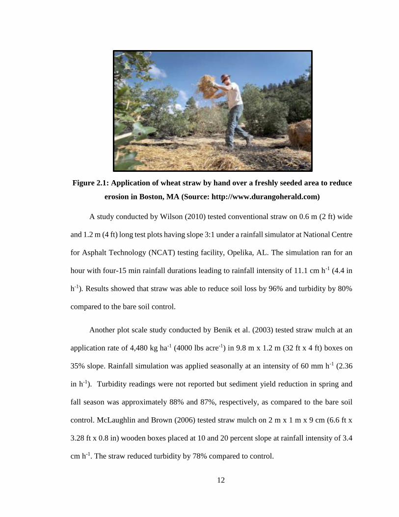
Agricultural straw is widely used in erosion control as a mulch. Moreover,

agricultural straw is inexpensive and easier to spread by hand or machine (Foltz and

Dooley, 2003). Typical application of wheat straw by hand is shown in Figure 2.1 for

erosion control in Boston, MA. Agricultural straw is used in the forested areas of the US

for erosion control on hill slopes, cuts and fills and other disturbed areas (Robichaud et al.,

2000). Straw provides a high degree of cover to reduce the impact of raindrops and prevent

soil particle detachment (Broz et al. 2003). The long stems of straw act as a mechanism to

reduce overland water velocity while capturing sediment already in motion (Foltz and

Dooley, 2003). However, straw decomposes over a relatively short time, thus reducing its

effectiveness in subsequent rain events (Wishowski et al., 1998).

Mulch Rate (Metric tons ha-1) Guidelines

Conventional

straw with seed

3.4-4.5 Spread by hand or machine to attain 75%

groundcover; anchor when subject to

blowing.

Conventional

straw (No Seed)

5.6-6.7 Spread by hand or machine; anchor when

subject to blowing.

Wood chips 11.2-13.5 Treat with 12 lbs. nitrogen/ton.

Bark 26.8 cubic yards Can apply with mulch blower

Pine straw 2.2-4.5 Spread by hand or machine; will not blow

like straw.

Peanut hulls 22-44 Will wash off slopes. treat with 12 lbs.

nitrogen/ton.

12

A study conducted by Wilson (2010) tested conventional straw on 0.6 m (2 ft) wide

and 1.2 m (4 ft) long test plots having slope 3:1 under a rainfall simulator at National Centre

for Asphalt Technology (NCAT) testing facility, Opelika, AL. The simulation ran for an

hour with four-15 min rainfall durations leading to rainfall intensity of 11.1 cm h-1 (4.4 in

h-1). Results showed that straw was able to reduce soil loss by 96% and turbidity by 80%

compared to the bare soil control.

Another plot scale study conducted by Benik et al. (2003) tested straw mulch at an

application rate of 4,480 kg ha-1 (4000 lbs acre-1) in 9.8 m x 1.2 m (32 ft x 4 ft) boxes on

35% slope. Rainfall simulation was applied seasonally at an intensity of 60 mm h-1 (2.36

in h-1). Turbidity readings were not reported but sediment yield reduction in spring and

fall season was approximately 88% and 87%, respectively, as compared to the bare soil

control. McLaughlin and Brown (2006) tested straw mulch on 2 m x 1 m x 9 cm (6.6 ft x

3.28 ft x 0.8 in) wooden boxes placed at 10 and 20 percent slope at rainfall intensity of 3.4

cm h-1. The straw reduced turbidity by 78% compared to control.

Figure 2.1: Application of wheat straw by hand over a freshly seeded area to reduce

erosion in Boston, MA (Source: http://www.durangoherald.com)

13

In 2003, Bjorneberg et al. tested six different treatments in 1.5 m x 1.2 m x 0.2 m

(4.9 ft x 3.9 ft x 8 in) steel boxes filled with loam soil on a 2.4% slope. Irrigation water was

appplied with a Veejet Nozzle (8070) at 80 mm h-1 (3.15 in h-1) for 15 minutes. Straw was

applied at two different covers 30% and 70% at a rate of 670 kg ha-1 (600 lbs acre-1) and

2500 kg ha-1 (2230 lbs acre-1), respectively. 70% straw cover reduced runoff and sediment

loss by more than 80% and 95%, respectively and 30% straw cover reduced runoff and

sediment loss by 52% and 51%, respectively.

Kukal and Sarkar (2010) studied the effect of wheat straw and polyvinyl alcohol

(PVA) solution on splash erosion and infiltration rate in two different soils under simulated

rainfall in semi-arid tropics. They treated the tilled soil surface with chopped wheat straw

at the rate of 6 ton ha-1 with sprayed 0.1% to 0.5% PVA solution. The average soil loss on

the wheat straw treatment was decreased by 56% and 84% with 0.1% PVA and 0.5% PVA,

respectively. Results showed that wheat straw and PVA was more effective in decreasing

erosion and increasing infiltration in sandy loam than in silt loam. Jiang et al. (2011)

investigated the effect of wheat straw mulch on runoff and erosion in the Midwestern

United States. Straw in their study reduced runoff and soil erosion by 68% and 95%,

respectively, compared to bare soil.

A rainfall simulator study was carried out by Groen and Woods (2008) to compare

the erosion and runoff rates from 0.5 m2 (5.4 ft2) plots with wheat straw and aerial seeding

in July, 2002 in northwest Montana. Wheat straw at an application rate of 2240 kg ha-1

(1998 lbs acre-1) resulted in 100% ground cover and 87% reduction in erosion compared

to the bare soil control. Table 2.2 summarizes the straw mulch literature.

14

Table 2.2: Summary of straw mulch literature

Study Test-Scale Application rate

(kg ha-1)

Reduction (%)

Soil loss Turbidity

Wilson (2010) Small 4,480 96 80

Benik et al. (2003) Large 4,480 88

Mclaughlin and

Brown (2006)

Small 2,200 UNK1 78

Bjornenerg et al.

(2003)

Small 670

2,500

51

95

UNK

Jiang et al. (2011) Small 6,000 95 UNK

Groen and Woods

(2008)

Small

2,240

87 UNK

1Unknown

2.5 Hydraulically applied mulch for erosion control

Field practices such as blown straw and straw mulch can be least expensive and

reliable form of erosion control whereas the application of hydraulically applied mulch

(Figure 2.2) provides to be efficient in terms of performance to provide the highest level of

erosion control on disturbed soils (Lipscomb et al., 2006).

Figure 2.2: Hydra CX2® hydromulching operation in the field for erosion reduction

(Source: www.fostersupply.com)

15

Hydraulically applied mulches have shown great improvement over the past 50 years

in terms of technological advancement and increased environmental awareness and have

become an efficient and widely used tool for erosion control, bank stabilization and

vegetation establishment (Wilson, 2010). Erosion control technology council (ECTC) has

divided hydraulically applied erosion control products (HECPs) into four different

categories based on functional longevity, erosion control effectiveness, and vegetation

establishment (Table 2.3). “As a general rule, the more expensive hydromulches, such as

bonded fiber matrices (BFM), tend to offer better protection against erosion, but actual results

are site specific” (Babcock and McLaughlin, 2008). “Hydraulic mulches lack appreciable

tensile strength, shear strength and life span, their use generally is limited to flatter and shorter

slopes with very low overland flows” (Lancaster and Austin, 2004).

Table 2.3: Various types of HECPs (Babcock and McLaughlin, 2008)

Slope

Ratio Material Rate

(kg ha-1) Description

≤2H:1V Stabilized

Mulch

Matrix

(SMM)

1,680-2,800 Organic fibers with soil flocculants or cross-linked

hydro-colloidal polymers or tackifiers. Used to

provide erosion control and facilitate vegetative

establishment on moderate slopes. Designed to be

functional for a minimum of 3 months.

≤2H:1V Bonded

Fiber

Matrix

(BFM)

3,360-4,480 Organic fibers and cross-linked insoluble hydro-

colloidal tackifiers. Used to provide erosion control

and facilitate vegetative establishment on steep

slopes. Designed to be functional for a minimum of

6 months. May need 24 hr cure time.

≤2.5H:1V Fiber

Reinforced

Matrix

(FRM)

3,360-5,040 Organic defibrated fibers, cross-linked insoluble

hydro-colloidal tackifiers, and reinforcing natural or

synthetic fibers. Used to provide erosion control and

facilitate vegetative establishment on very steep

slopes. Designed to be functional for a minimum of

12 months.

≤6H:1V Hydraulic

Mulch

(HM)

1,680 Paper, wood or natural fibers that may or may not

contain tackifiers. Used to facilitate vegetative

establishment on mild slopes. Designed to be

functional for up to 3 months.

16

McLaughlin and Brown (2006) tested straw, straw erosion control blanket and two

mechanically bonded fiber matrix (MBFM) hydromulches with PAM in 100 cm (39 in)

wide, 200 cm (78 in) long and 9 cm (3.5 in) deep test plots. Two tests were conducted: 1)

a 4% slope under natural rainfall, and, 2) 10% to 20% slopes using rainfall simulator

intensity of 3.4 cm h-1 (1.3 in h-1). A commercial hydroseeder was used to apply MBFM at

3363 kg ha-1 (3000 lbs. acre-1). Results showed that the application of MBFM without PAM

reduced average turbidity by approximately 85% and sediment loss by 86% compared to

bare soil control under natural rainfall and 96% turbidity reduction under simulated rainfall.

Benik et al. (2003) conducted a study to evaluate the effectiveness of bonded fiber matrix

(BFM) treatment. The application rate for BFM was 3363 kg ha-1 (3000 lbs. acre-1) with a

24 hour drying period, per manufacturer’s specifications. Results showed that the Soil

Guard® BFM reduced average sediment yield by 94% compared to bare soil.

Plot scale study conducted by Wilson (2010) tested four different hydromulches, (1)

Excel® Fibermulch II, (2) GeoSkin®, (3) HydraCX2®, and (4) HydroStraw® BFM and

compared their performance with two conventional straw practices, crimped and tackified,

with bare soil as a control on a 3:1 slope using a rainfall simulator with a rainfall intensity

of 11.1 cm h-1 (4.4 in h-1) in 1.2 m x 0.6 m (4 ft x 2 ft) test plots. Cover factor (C factor)

was also calculated to determine performance of each cover. Cover factor is the parameter

used in revised universal soil loss equation representing a soil loss occurring within the

treatments compared to bare soil, unprotect condition (Clopper et al. 2001). Results showed

that the Hydro Straw BFM (C factor= 0.04) was the most effective treatment having 99%

average turbidity reduction and 100% sediment reduction, as compared to the bare soil

control. HydraCX2 (C factor = 0.013) was the second best hydromulch treatment with 95%

17

turbidity reduction and 99% sediment reduction, as compared to the bare soil control

followed by GeoSkin (C factor = 0.028) with 92% reduction in turbidity and 97% sediment

reduction, as compared to the bare soil control. Excel Fibermulch II (C factor = 0.068) had

85% turbidity reduction and 94% sediment reduction, as compared to the bare soil control.

The stabilization performance of two compost wood mulch blends, a wood based

hydromulch and a bare soil to determine the amount of sediment from each treatment was

compared by Bradley et al. (2010). Test plots of 12.2 m x 2.4 m (40 ft x 8 ft) were

constructed and runoff was evaluated for two years after installation. Results showed that

the hydromulch at an application rate of 2242 kg ha-1 (2000 lbs acre-1) reduced sediment

yield by 75% compared to bare soil. Prats et al. (2013) applied hydromulch at3500 kg ha-1

(3000 lbs acre-1) consisted of a mixture of organic fibers, water, and seed to reduce runoff

and erosion from burnt pine planation in central Portugal. Results concluded that

hydromulch reduced runoff volume by 70% and soil erosion by 83%, as compared to bare

soil.

Holt et al. (2005) performed an experiment on six hydromulch treatments, all tested

in 0.6 m (2 ft) wide, 3.05 m (10 ft) long and 0.076 m (3 in) deep trays with a sandy loam

soil. Six hydromulch treatments, including wood hydromulch, paper hydromulch,

cottonseed hulls hydromulch, cotton by product (COBY) hydromulch produced from

stripper waste (COBY Red), COBY produced from ground stripper waste (COBY green)

and COBY produced from picker waste (COBY green) were tested on packed and leveled

soil at 15.7% slope with a rainfall simulation intensity of 6.35 cm h-1 (2.5 in hr-1). Patented

cotton hydromulch made from cottonseed hulls is known as COBY (Hold and Laird, 2002).

Hydromulches were applied by hand at 1,120 kg ha-1 (1,000 lbs acre-1) and 2,241 kg ha-1

18

(2,000 lbs acre-1). Results showed that COBY green, COBY red, COBY yellow, cottonseed

hulls , paper and wood hydromulches yielded a cover factor of approximately 0.20 and

0.32, 0.10 and 0.22, 0.20 and 0.22, 0.16 and 0.21, 0.42 and 0.68, and 0.65 and 0.81 at 1120

kg ha-1 and 2241 kg ha-1, respectively. Gabriel (2009) tested the performance of a

hydromulch on 2 m x 8 m (6.6 ft x 26 ft) with application rate of 3,900 kg ha-1 (3,500 lbs

acre -1) on 3:1 slope at San Diego State University's Soil Erosion Research Laboratory. The

high performance hydromulch produced a C factor of 0.002 with 99.8% effectiveness.

Landloch (2002) tested four different hydromulch treatments including paper

hydromulch, flax hydromulch, flax plus paper hydromulch and sugarcane hydromulch,

applied at a rate of 1,000 kg ha-1 (893 lbs acre-1), 2,500 kg ha-1 (2232 lbs acre-1), 3,250 kg

ha-1 (2,900 lbs acre-1) and 5,000 kg ha-1 (4,464 lbs acre-1), respectively. Test plots were 5

m (16.4 ft) long and 1.5 m (4.9 ft) wide at a 25% slope on alluvial black, cracking clay soil.

Simulated rainfall was applied at an intensity of 14.4 cm h-1 (5.7 in h-1) for 20 minutes to

match the 10 year storm event. Cover factors for paper, flax, flax plus paper and sugarcane

hydromulches were reported as 0.204, 0.149, 0.044 and 0.037, respectively.

2.5.1 Hydroseeding for erosion control

Hydroseeding is the technique that is often used on steep slopes and areas for vegetation

establishment (Enriquez et al., 2004). Hydroseeding consists of mixing seed, fertilizers,

water and other substances into an applied slurry, which is applied to prepared seed bed to

promote vegetation establishment. Hydroseeding can achieve dense vegetation cover in the

short term by stabilizing the soil, thus controlling erosion (Merlin et al., 1999; Robichaud

et al., 2000). Hydroseeding had been widely used for vegetation establishment on road fills

19

in Spain but in semi-Mediterranean climate the technique did not produced expected results

in establishing a dense vegetative cover (Muzzi et al., 1997; Bochet and Fayos 2004).

Dougherty et al. (2008) tested six cover treatments and one bare soil treatment on 3 m

by 7.6 m (10 ft x 25 ft) outdoor plots in Auburn, AL. Seed, lime and fertilizers were mixed

as slurry in two of the hydromulch treatments and incorporated in the soil in other two

hydromulch treatments. Results proved that incorporation of seed before hydromulching

operation was an effective vegetation establishment measure with 30-fold sediment

reduction compared to the bare soil plot. The study also reported that the incorporation of

lime, fertilizers and seed in the Geoskin™ hydromulch treatment resulted in a 48%

reduction in total sediment yield over the corresponding treatment in which seed, lime, and

fertilzer was not incorporated.

Montoro et al. (2000) tested the effectiveness of hydroseeding techniques with the

application of vegetal mulch, hydroseeding with added humic acid, hydroseeding with

vegetal mulch and added humic acid and a control without hydroseeding or soil

amendment. They found that all the hydroseeding treatments significantly reduced runoff

and soil loss and that vegetal mulch with added humic acid was most effective (98.5%

reduction of total soil loss versus 95% for other treatments). Table 2.4 summarizes the

hydromulch literature.

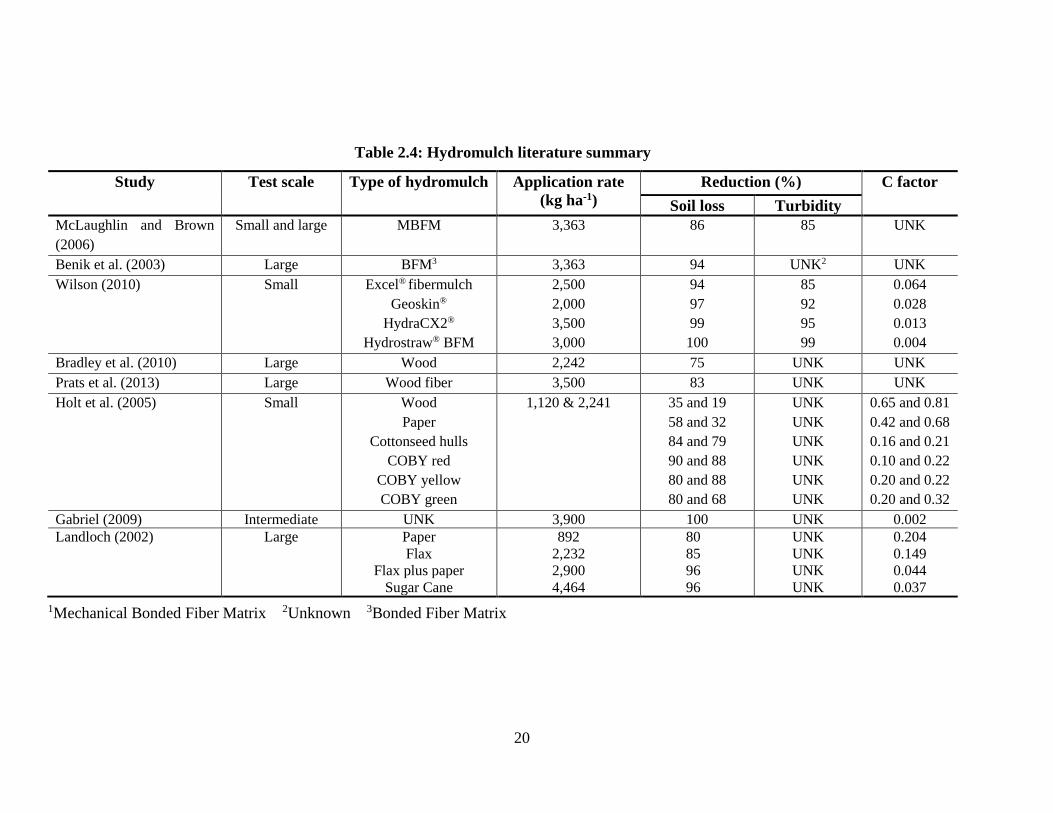
20

Table 2.4: Hydromulch literature summary

Study Test scale Type of hydromulch Application rate

(kg ha-1)

Reduction (%) C factor

Soil loss Turbidity

McLaughlin and Brown

(2006)

Small and large MBFM 3,363 86 85 UNK

Benik et al. (2003) Large BFM3 3,363 94 UNK2 UNK

Wilson (2010) Small Excel® fibermulch

Geoskin®

HydraCX2®

Hydrostraw® BFM

2,500

2,000

3,500

3,000

94

97

99

100

85

92

95

99

0.064

0.028

0.013

0.004

Bradley et al. (2010) Large Wood 2,242 75 UNK UNK

Prats et al. (2013) Large Wood fiber 3,500 83 UNK UNK

Holt et al. (2005) Small Wood

Paper

Cottonseed hulls

COBY red

COBY yellow

COBY green

1,120 & 2,241 35 and 19

58 and 32

84 and 79

90 and 88

80 and 88

80 and 68

UNK

UNK

UNK

UNK

UNK

UNK

0.65 and 0.81

0.42 and 0.68

0.16 and 0.21

0.10 and 0.22

0.20 and 0.22

0.20 and 0.32

Gabriel (2009) Intermediate UNK 3,900 100 UNK 0.002

Landloch (2002) Large Paper

Flax

Flax plus paper

Sugar Cane

892

2,232

2,900

4,464

80

85

96

96

UNK

UNK

UNK

UNK

0.204

0.149

0.044

0.037

1Mechanical Bonded Fiber Matrix 2Unknown 3Bonded Fiber Matrix

21

2.6 PAM for erosion control

In 1950s, a low molecular weight polyacrylamide (PAM) was introduced in

agricultural market to control soil erosion, but mixing of PAM with soil was expensive.

Therefore, the product disappeared from the market. It was later introduced in the late

1980s with the advancement in polymer chemistry to control erosion in furrow-irrigated

agriculture. It generally increases infiltration by preserving a more pervious pore structure

(Sojka and Lentz, 1996) but effects varied with soil texture (Sojka et al., 1998). The net

increase of infiltration on fine textured soils was higher using PAM and infiltration rates

increased by 15% on a Portneuf silt loam soil (Sojka et al., 1998). Polyacrylamide increased

and preserved surface aggregate structure, with reduced surface crusting, increased

infiltration and decreased runoff volume (Sojka et al. 2007; Green et al., 2000; Vacher et

al. 2003; Yu et al. 2010; Flanagan et al. 2002a; 2002b).

Polyacrylamide can be an effective erosion and sediment control technique for

reducing soil loss, decreasing runoff volume, increasing infiltration, preventing surface

crusting (Akbarzadeh et al., 2009; Babcock and McLaughlin, 2011; Flanagan et al., 2002a,

2002b; Green et al., 2000; Zhang et al., 1998). Polyacrylamide effectiveness varies by

application rate and soil conditions. The cost of PAM application on steep slopes (80 kg

ha-1) ranged from $265-550 ha-1 less than the cost of other straw mulch products (Flanagan

and Chaudhari, 1999). So, PAM can be an effective cost saving measure in controlling

erosion and increasing vegetation establishment on construction sites. Figure 2.3 shows the

effect of PAM in sediment laden water.

Polyacrylamide has three different forms: emulsive, solutions, and dry granules.

Liquid PAM has been shown to increase soil infiltration up to 1.7 to 2.8 times compared

22

with non-PAM controls (Yu et al., 2010). Dry granular PAM spread on the soil surface was

more effective in increasing infiltration than mixing dry granular PAM in to the top soil

with soil erosion was decreased by 80% compared to the control (Yu et al., 2010). Liquid

PAM applied and then dried on the soil surface was the most effective in reducing runoff

by 62% to 76% and sediment yield by 93% to 98%, as compared to a non-PAM control

(Peterson et al., 2002).

(Without PAM) (With PAM)

Shoemaker (2009) tested the dry granular PAM product known as Silt Stop 712

(Applied Polymer Systems, Woodstock, GA) with application rates of 16.8, 27.9, and 39.2

kg ha-1 (15, 25 and 35 lbs acre-1) on untreated, unseeded 1.2 m x 0.6 m (2 ft x 4 ft) laboratory

scale test plots. Polyacrylamide treatment applied at recommended application rate of 39.2

kg ha-1 (15 lbs acre-1) was able to reduce turbidity by 97% and net soil loss by 50%, as

compared to bare soil control. Results indicate that dry PAM applied at the recommended

application rate kept eroded soil from washing away by reducing detachment.

Figure 2.3: Effect of PAM upstream on sediment laden water

(Source: http: //www. ucanr.edu)

23

Some researchers had reported mixed results with PAM. Soupir et al. (2004)

reported that PAM applied as a dry powder at 20 kg ha-1 (18 lbs acre-1) on large scale (28

m x 2 m) plots reduced TSS by 50% compared to control. Zhang et al. (1998) found that

application of 20 kg ha-1 PAM on a 6% slope reduced runoff volume by 44% and soil loss

by 19% over a five month period. Past research suggest that a minimum application rate of

22 kg ha-1 is required for any benefit in reducing erosion (McLaughlin, 2006) but

application rate below 22 kg ha-1 can be effective in erosion control and requires further

research.

A study conducted in Iran by Sepaskhah and Bazrafshan-Jahromi (2006) used 1.4

m x 1.4 m (4.5 ft x 4.5 ft) steel boxes with a depth of 0.09 m (3.5 in) with 2.5%, 5%, and

7.5% slopes. A flume was constructed downslope to divert runoff to a collection point. A

PAM treatment was applied at 1, 2, 4, and 6 kg ha-1 and was subjected to sprinkler

irrigation. Researchers concluded that treatment with a steeper slope required a higher

application rate of PAM to reduce erosion. The study also concluded that PAM treatments

were more effective in reducing sediment erosion, rather than reducing runoff volume.

Polyacrylamide was effective in reducing soil loss, with the higher rate of PAM (40

kg ha-1) having less soil loss than that from a lower rate of PAM (20 kg ha-1) at slopes of

20% and 40%. (Lee et al., 2011). Partington and Mehuys (2005) found that PAM applied

at 10 kg ha-1 and 20 kg ha-1 (9 lbs acre-1 and 18 lbs acre-1) was inadequate to control erosion

after natural rainfall on a loam soil. They conducted a similar experiment under simulated

rainfall conditions and found that PAM applied at 10 kg ha-1 and 20 kg ha-1 (9 lbs acre-1

and 18 lbs acre-1) on silt loam soil reduced soil erosion by 84% and 76%, respectively, and

turbidity of runoff water by 99%.

24

Zhang et al. (1998) found that 20 kg ha-1 (18 lbs acre-1) of PAM applied in

conjunction with gypsum on a very low slope reduced runoff by 44% compared to a non-

PAM control. Application of PAM reduced runoff continuously compared to the control

for up to 160 days after application by 35%. Polyacrylamide application reduced the runoff

volume significantly by 94% and 90% in the first and second storms, respectively, but

resulted in only 17% reduction in soil loss compared to a non-PAM bare soil in the fourth

month of the experiment.

Flanagan et al. (2002a) tested PAM, PAM plus gypsum and untreated control on

nine 9.14 m x 2.96 m (30 ft x 9.7 ft) long erosion plots in West Lafayette, Indiana under

simulated rainfall. The application of PAM (80 kg ha-1) and 5 Mg ha-1 (4461 lbs acre-1)

gypsum significantly reduced runoff and sediment yield by 52% and 91%, respectively,

compared to control on a 32% slope. Total soil loss was reduced in the range of 40% to

54% compared to control when applied at the same application rate on 35% and 45% slope

under natural rainfall. They found that application of PAM and PAM with gypsum

protected the soil during the period of vegetation growth for disturbed soils on steep slopes

more than non-PAM control. Table 2.5 is the summary of PAM literature.

Table 2.5: PAM literature summary

Study Test Scale Application rate

(kg ha-1)

Reduction (%)

Soil loss Turbidity

Shoemaker (2009) Small 39 50 97

Soupir et al. (2004) Large 20 50 UNK1

Zhang et al. (1998) UNK 20 19 UNK

Partington and

Mehuys (2005)

UNK 20 76 99

Flanagan et al.

(2002a)

Large 80* 91** UNK

1Unknown *Gypsum was added (5 Mg ha-1) **32% slope

25

2.6.1 PAM with wheat straw for erosion control

Several Studies were tested using PAM in combination of wheat straw. Bjorneberg

et al. (2000) tested PAM and PAM with wheat straw in steel boxes of 1.5 x 1.2 m x 0.2 m

(5 ft x 4 ft x 0.6 ft) irrigated at 80 mm h-1 (3.4 in h-1) for 15 minutes. Wheat straw was

applied at 2500 kg ha-1 (2230 lbs acre-1) by visually estimating a 70% and 670 kg ha-1 (600

lbs acre-1) for 30% straw cover with PAM applied at 2 and 4 kg ha-1 (1.8 and 3.6 lbs acre-

1) in both the straw treatments. Results showed that 70% wheat straw cover with PAM (2

kg ha-1) reduced runoff and sediment loss by 98% and 99%, respectively compared to bare

soil. 30% straw cover with PAM (2 kg ha-1) reduced runoff and sediment yield by 53% and

82%, respectively compared to bare soil. 70% straw cover with PAM (4 kg ha-1)

significantly reduced soil loss by almost 100% compared to bare soil than 70% straw with

2 kg ha-1 PAM.

Lentz and Bjorneberg (2003) tested wheat straw treatment with PAM in

conventially irrigated furrows. Five irrigations were performed on a 1.5% slope silt loam

soil. Polyacrylamide and straw reduced sediment loss by 64% to 100% in all the irrigations.

Adding PAM to low (485 kg ha-1) and high (1490 kg ha-1) application rates of straw

treatment increased sediment loss reduction from 80% to 100% in the first two irrigations

and from 94% to 99.8% in subsequent irrigations.

PAM used with seed and mulch had been effective in reducing runoff and turbidity.

An experiment conducted by Hayes et al. (2005) showed that PAM used in conjunction

with seed and mulch significantly decreased turbidity and sediment loss from plots

compared with PAM alone. Seed/mulch with PAM reduced 83% erosion when compared

to 42 ton ha-1 rate of bare soil from a single storm event. Roa-Espinosa et al. (1999) tested

26

PAM with straw and PAM alone in 1 m x 1m (3.28 ft x 3.28 ft) plots on 10% slope.

Simulated rainfall with an intensity of 6.32 cm h-1 (2.5 in h-1) was applied over each

treatment. Results reported that a treatment of 22.5 kg ha-1 (20 lbs acre-1) PAM and mulch

applied to dry soil reduced sediment loss by 93% compared to control. Dry PAM reduced

the sediment yield by 83% compared to control.

Flanagan and Canady (2006) tested the effectiveness of PAM on 4% and 8% slopes

with two wheat straw cover levels of 0% and 30% under a rainfall simulator. The

experiment was conducted in aluminum boxes measuring 31 cm (12 in) wide, 45 cm (18

in) long, and 30 cm (12 in) deep. Two different storms were simulated, with the first storm

using a duration of 1 hour with a constant intensity of 64 mm h-1 (2.5 in h-1). A second

storm had varying intensities of 64, 94 and 25 mm h-1 (2.5, 3.7 and 0.98 in h-1) in sequential

20 min increments. Results showed that PAM in conjunction with wheat straw reduced

runoff up to 66% compared to bare soil control.

2.7 Vegetation for erosion control

The presence of vegetation has shown to be effective tool in reducing runoff and

sediment loss (Marques et al. 2007). Vegetation reduces water induced erosion by

intercepting rainfall, increasing the infiltration rate of the soil, intercepting runoff at the

soil surface and stabilizing the soil with roots (Gyssels et al., 2005), resulting in lower soil

detachment energy (Bochet and Fayos, 2004). The cover factor value of Universal soil loss

equation for fallow land is 1 and for a permanent cover, C factor value is 0.001. This

indicates that the same soil under a permanent grass cover is 1000 times less erosive than

bare soil (Troeh and Thompson, 2005).

27

Cover crops were grown to provide cover in winter and fallow conditions during annual

cropping systems (Meerkerk, 2008). Several studies reported on the use of cover crops as

erosion control measures (Kaspar et al., 2001; Malik et al., 2000). Four species of cover

crop including ryegrass (Lolium), crimson clover (Trifolium incarnatum), Sericea

lespedeza (Lespedeza cuneata) and tall fescue (Festuca arundinacea) reduced soil erosion

by about 64%, 61%, 51% and 37%, respectively, compared to bare soil in the early

development of a short rotation woody crop plantation (Malik, et al., 2000).

Plots seeded with annual ryegrass (Lolium Multiflorum.) had 31% less sediment loss as

compared with non-seeded plots (Gautier, 1983). Zhou and Shangguan (2007) conducted

four rainfall simulator experiments with rainfall intensity of 1.5 mm min-1 (0.59 in min-1)

to investigate the effect of ryegrass (Lolium) on runoff and soil loss and found that runoff

decreased 25% and 70%, respectively, after the 12th and 27th week of planting in ten

ryegrass pans, 2.0 m (6.6 ft) long, 0.28 m (0.9 ft) wide, and 0.35 m (1.15 ft) deep. Sediment

reduction compared to bare soil amounted to 95% in the 27th week. Mitchell et al. (2003)

reported that perennial ryegrass (Lolium perenne) reduced erosion by 46% compared to the

bare soil.

Pan and Shangguan (2006) conducted an experiment on different percent of grass cover

(35%, 45%, 65% and 90%) of Perennial black ryegrass (Lolium perenne L.) and found

runoff reduction of 14%, 25%, 16%, and 21% and sediment loss reduction of 81%, 85%,

87% and 94% at 35%, 45%, 65% and 90% cover, respectively, compared to bare soil. Liu

et al. (2010) performed a similar experiment to reduce erosion on loess plateau in China.

They constructed artificial road sections packed with the soil from the plateau and planted

differing grass covers (0%, 30%, 40%, 50%, 60% and 70%) of Kentucky bluegrass (Poa

28

Pratensis) with simulated rainfall at 120 mm hr-1 (4.7 in h-1) for 1 hour. Increasing grass

cover inhibited overland flow, increased friction and surface roughness and reduced mean

flow velocities. Runoff and sediment from grass covered plots were reduced from 12.4%

to 27.9% and 39% to 76%, respectively with increase in percent vegetation cover,

compared to bare soil.

Gross et al. (1991) tested different seeding rates at 98, 244, 390, and 488 kg ha-1 (87,

218, 348 and 435 lbs acre-1) of tall fescue (Festuca arundinacea) with different rainfall

intensities of 76, 94 and 120 mm h-1 (3, 3.7 and 4.7 in h-1). Results reported that at high

rainfall intensity (120 mm h-1), the sediment loss was reduced six times at 98 kg ha-1

seeding rate compared with control. There were no significant differences in sediment loss

across all seeding rates at medium and low rainfall intensity. Fox et al. (2010) conducted

plot scale field trails consisting of Japanese millet (Echinochloa esculenta) and buffel grass

(Cenchrus Ciliaris) to control erosion on slopes of railway embankment and found that

after 63 days of seeding, millet alone reduced soil erosion by 50% as compared to buffel

grass alone. Soil loss was reduced by 90% compared to the bare soil control as a result of

over 60% grass cover from all the seeded treatments established after 11 months of

planting.

Grace (2002) tested the effectiveness of wood excelsior, native vegetation and exotic

vegetation in erosion control for forest road side slopes in the Talladega National Forest in

Alabama over a 4-year period in 12 plots of 1.5 m x 3.1 m (5 ft x 10 ft). The native species

mixture included big bluestem (Andropogon gerardii), little bluestem (Schizachyrium

scoparium), and Alamo switch grass (Panicum virgatum). The exotic species mixture

consisted of Kentucky 31 tall fescue (Festuca arundinecea), Pensacola bahiagrass

29

(Paspalum notatum), Annual lespedeza (Lespedeza cuneata), and white clover (Trifolium

repens). Sediment and runoff yield was significantly reduced by vegetation compared with

the bare soil control. Mean sediment yield from native species, exotic species and erosion

mats was 1.1, 0.45 and 0.80 g m-2 mm-1, (251, 100 and 178 lbs acre-1 in-1) respectively.

2.7.1 Vegetation with temporary erosion control covers

Temporary vegetation with erosion control covers proved to be a cost effective

temporary stabilization and erosion control method (Idaho BMP manual, 2014). Lemly

(1982) tested five different treatments including asphalt-tacked straw, jute netting, mulch

blanket, wood chips and Curlex® Excelsior blanket seeded with 2 kg ha-1 (1.8 lbs acre-1)of

tall fescue. All the treatments reduced erosion by approximately 75%, as compared to the

bare soil control. Grass coverage was significantly increased by the introduction of all the

treatments and results showed that all treatments obtained grass coverage of approximately

75% within three months after seeding. Bare soil plots had only 40% cover in same period.

Megahan et al. (2006) studied different erosion control practices on granitic road fills

for forest roads in Idaho. They used different plots 1-8 m (3-26 ft) wide and 4-6 m (13-20

ft) long to calculate runoff. They found that combining mulch with vegetation was a more

effective erosion control measures than mulch alone or vegetation alone. Xin-Hu et al.

(2011) conducted an experiment to determine runoff and soil loss from a 5 m x 15 m (16

ft x 49 ft) plot for a duration of five years (2001-2005) using cover (Bahiagrass), mulch

and bare soil. They found that Bahiagrass (Paspalum notatum) and mulch plots had less

erosion and runoff compared to bare soil and suggested that Bahia grass cover was

excellent as it is easier to use and therefore a feasible practice for soils in Southern China.

30

Dougherty et al. (2008) found out that 75% establishment of Bermudagrass cover took

approximately 90 days from seeding. Three general stages of vegetation growth including:

1) 0% to 50% cover providing the highest sediment yield (0-45 days after seeding) 2) 50%

to 75% with moderate sediment yield (50-60 DAS) 3) 75% to 100% were reported with

lowest sediment yield (> 80 DAS). Dougherty et al (2010) found that adding PAM

hydromulch did not significantly improve seeding grass establishment when compared to

a non-PAM hydromulch treatment. Hydromulch was more effective than erosion control

blanket or loose straw treatments in terms of grass establishment.

Baharanyi (2010) tested the differences in Bermudagrass establishment with

temporary covers like wheat straw, erosion control blankets, and hydromulch with and

without PAM. He found that after the first 90 days of planting, PAM application had no

effect on Bermudagrass establishment and Bermudagrass was established quicker with

hydromulch, compared with loose straw or erosion control blankets.

2.7.2 Line point intercept method for vegetation cover determination

There are several methods to determine the extent of vegetation cover, including

point based sampling and line intercept sampling method. The standard alternative to the

point based sampling method is the line intersect sampling method (Jennings et al., 1999,

Williams et al., 2003). The points on the line where the canopy cover begins and ends are

recorded using tape measure and percentage cover is calculated by number of points hitting

the canopy projecting from the top to the total number of points in a transect. The lines

should be placed in either systematic or random way covering the entire plot (Jennings et

al., 1999, Williams et al., 2003).

31

Godinez-Alvarez et al. (2009) used the line point intercept method along a 70 m

(230 ft) baseline with four 70 m (230 ft) transects spaced equally 10 m (33 ft) apart to

analyze foliar cover in the Chihuahuan Desert in Mexico. Cover was recorded after every

1 m, with 70 points per transect. Percent cover as measured from the line transect method

was significantly higher than subjective visual estimates. Weltz et al. (1994) used the line

intercept point transect method in a 20 pin vertical point frequency frame on 0.5 m x 1 m

(1.6 x 3.2 ft) quadrats located along line intercept transects. Three 20 point pin frames were

evaluated, resulting in a total of 60 points. Plant height, canopy cover and canopy diameter

were estimated using this method.

Ruthven et al. (1993) used the line intersect method to estimate woody plant canopy

cover with twenty five transects ranging from 72 to 351 m (236 to 1152 ft) long with four

20 m (66 ft) lines placed along and perpendicular to the transect, leading to a total of 100

points per site. Booth et al. (2006) used a sighting device or pin to read points along the

transect. Readings were recorded observing the color at every 10 cm (0.33 ft) increment on

a tape stretched along the transect.

Etchberger and Krausman (1997) studied five different methods, including the line

intercept method, to sample desert vegetation Tumamoc Hill, Pima County, Arizona. Four

30 m (98 ft) transects were randomly placed at 12 points, a total of 40 transects. The total

vegetation cover was calculated not by measuring the length of vegetation canopy

intercept, but by dividing the total number of hits for a plant species by the total number of

hits for all species.

32

2.8 Rainfall simulator use in erosion control experiments

The use of rainfall simulators in erosion studies is not new (Young and Burwell,

1972). As researchers require erosion and sediment control experiments suitable for

repetitive testing, use of simulated rainfall to generate runoff has increased (Benik et al.,

2003; Bjorneberg et al., 2000; Flanagan et al., 1997; Flanagan et al., 2002a; McLaughlin

and Brown, 2006; Peterson et al., 2002; Roa-Espinosa et al., 1999; Sepaskhah and

Bazrafshan Jahromi 2006; Shoemaker, 2009; Wilson, 2010).

Cerda et al. (1997) used a nozzle, a structure in which the nozzle was installed and

connections with water supply and pumping systems. A wind protector to avoid

interference during the experiment was highly recommended. The nozzle was connected

directly to the pump by a single pipe. The height of the nozzle was 2 m (6.6 ft) above the

soil surface. The pumping system was operated mechanically or by hand. They found that

the most homogenous rainfall distribution was found at water pressure of 1.55 kg cm-2 (22

psi) and the rain intensity at this pressure was 54.6 mm h-1 (2.15 in h-1).

Esteves et al. (2000) designed and field tested a rainfall simulator for 5 m x 10 m

(16 ft x 32 ft) plots. The rainfall simulator was 6.58 m (22 ft) high with a 25.4 mm (1 in)

galvanized vertical standpipe. A nozzle was mounted at the end of the stand pipe which

sprayed a square area of 7 m x 7 m (23 ft x 23 ft). The spraying system nozzle was mounted

at a height of 6.53 m (21 ft) at the top of the pipe and the water was jetted to the height of

approximately 8 m (26 ft). An oil-immersed pressure gauge and cut off valve was installed

at the bottom of the pipe to achieve pressure control. Six rainfall simulators were combined

along two lines to spray the 50 m2 (538 ft2) plot. Guy ropes attached to stand pipes were

used to stabilize the system. The system was supplied by a pump from a storage tank near

33

the plots. Rainfall intensity was changed by adjusting water pressure. The rainfall intensity

produced by the rainfall simulator was 75 mm h-1 (3 in h-1) at a constant water pressure of

47.8 kPa (7 psi). Faucette et al. (2004) used eight V-jet nozzles in a rainfall simulator

obtained from the USDA National Soil Erosion Research Laboratory. The spray area of

the uniform rainfall with simulator was 6 m x 2 m (20 ft x 7 ft).

Miller (1987) used a portable, variable-intensity and low cost rainfall simulator in

runoff erosion studies that could be adapted for large plot studies for field use. Intensity

was varied from 0.0004 mm s-1 (0.056 in h-1) to 0.024 mm s-1 (0.34 in h-1) at 29 kPa (4.2

psi) water pressure by closing and opening electrically operated solenoid valve into which

wide square spray nozzles were fitted and controlled via switches operated by a rotating

cam or microcomputer. The coefficient of uniformity was 90% to 95% under a single

nozzle in a 1 m2 (10.76 ft2) field plot and 85% to 90% under a three nozzle system in a 1 x

3 m field plot. Similarly, Munn (1974) built a highly portable rainfall simulator to study

the erosion potential of different soil types in the Lake Tahoe Basin. Water was supplied

by a 20 L (5.3 gallon) jug attached to the top of the simulator. Rainfall occurred over 0.71

x 0.71 m (2.3 ft x 2.3 ft) square area and runoff was collected into collection jars from 0.61

x 0.61 m 9 2 ft x 2 ft) plots during 15 min long storms.

Grierson and Oades (1977) used a rainfall simulator mounted on a 1.8 x 1.2 m (6 ft

x 4 ft) steel trailer for a field study of erosion and runoff. A frame of steel tubing was used

to support the roof canopy and two side doors. Water was stored in two 200 L (53 gallon)

reservoirs mounted over the trailer. The nozzle was 2 m (6.6 ft) above the ground and rested

over a hole cut in the roof over the center of the plot with simulated rainfall intensity ranges

from 0.6 cm h-1 to 15 cm h-1. Freebairn and Gupta (1990) used a drop-former simulator on

34

0.91 m (3 ft) wide and 1.52 m (5 ft) long plots to study the role of cover, micro-topography

and antecedent rainfall on infiltration in fields subject to different tillage regimes in

Minnesota where corn had been continuously cropped for 3 years prior to the study. The

rainfall simulator was 2.5 m (8.2 ft) above the plots with simulation intesntiy of 100 mm

h-1 (4 in h-1) and runoff was measured by a tipping bucket mechanism. They found that

increased surface roughness decreased runoff when a surface cover was present.

Navas (1993) used a nozzle type simulator on 1.3 m x 1.3 m (4.1 ft x 4.1 ft) plots

to examine soil loss affected by different slopes, soil types and cover. Surface was wetted

in the first test with cover, and then the cover was removed during the second test, leaving

bare soil. Runoff was collected regularly at three-minute intervals. The study found that

runoff decreased with cover and increased with slope. Greene et al. (1994) used a trailer

mounted, nozzle type simulator over 1 m2 (10.76 ft2) plots to study the effect of plant cover

on runoff and erosion in Australia. Uniform runoff occurred for rainfall duration between

30 and 60 minutes. Runoff was collected with the help of a channel at the downslope end

by using a steel plot frame. They found that increased cover reduced runoff, but had no

effect on sediment concentration.

Roth et al. (1985) developed a simple and easily operated rainfall simulator for

infiltration research in Brazil. The water delivery structure was mounted at a height of 3 m

above the ground containing four water reservoirs. Drop size depended upon the different

tube diameters and rainfall intensity was verified between 0-185 mm h-1 (0-7.3 in h-1) by

adjusting water head in the reservoir. Rainfall intensify was 60% to 80% of the kinetic

energy of natural rainfall, calculated by an equation 2-1 developed by Foster et al. (1981).

𝑒 = 0.119 + 0.0873 log(𝑖) (2.1)

35

Where, i = intensity of rainfall (mm h-1)

e = rainfall energy (MJ ha-1 mm-1)

Martinez et al. (2001) constructed a rainfall simulator consisting of a square frame

with 2.5 m (8.2 ft) sides and supported by four pillars of 3.6 m (11.8 ft) to study change in

physical properties of the soil on 2 m x 2 m (6.6 ft x 6.6 ft) plots. They used two different

nozzles under pressures of 100 kPa (14.5 psi) and 90 kPa (13.05 psi) to produce rainfall

intensities of 33 mm h-1 (1.3 in h-1) and 60 mm h-1 (2.4 in h-1) , respectively.

Cornelis et al. (2004) studied the effect of wind and rainfall on soil erosion with the

help of a rainfall simulator and wind tunnel. The simulator was constructed with three pipes

attached to the sprinkler delivering pressurized water covering a 1.2 x 1.2 m (4 ft x 4 ft)

section. Arnaez et al. (2007) constructed a rainfall simulator with a sprinkler mounted at a

height of 2.5 m (8.2 ft) with pressurized water for 30 min simulations to compare runoff

and sediment production under different rainfall intensities in a vineyard plantation in

Spain. Three different rainfall intensities i.e. < 40, between 40 and 70 and >70 mm h-1 were

used with low intensity, intermediate intensity and high intensity nozzles, respectively.

Sheridan et al. (2008) used a rainfall simulator on 1.5 m x 2 m (5 ft x 6.6 ft) plots

to predict modified erodibility indices to estimate annual erosion rates for forest roads. The

rainfall intensity was fixed at 100 mm h-1 (3.9 in h-1) with a 30 min simulation and estimated

rainfall energy of 0.295 MJ ha-1 mm-1 as calculated by an equation 2.1 developed by Fosters

et al. (1981), was found to be similar to the energy of a high intensity rainfall. Table 2.6

summarizes the important literature of rainfall simulator.

36

Table 2.6: Important rainfall simulator literature summary

Study Test plots Nozzle height

(m)

Rainfall Intensity

(cm h-1)

Cerda et al. (1997) UNK1 2 5.5

Esteves et al. (2000) Large 6.5 7.5

Grierson and Oades

(1977)

Small 2 0.6-15

Freebairn and Gupta

(1990)

Small 2.5 10

Roth et al. (1985) UNK 3 0-19

Martinez et al. (2001) Small 2.5 3.3-6

Arnaez et al. (2007) UNK 2.5 <4, 4-7, and >7 1Unknown

2.9 Cost of erosion control BMPs in previous studies

Jin and Englande (2008) tested five erosion control measures againsta bare soil as

control in Louisiana, US. The cost of temporary seeding used in the study was $0.20 per

92 m2 (990 ft2) and cost of straw bedding was $5 per 92 m2 (990 ft2). The most cost effective

treatment was temporary seeding using perennial ryegrass, with 10.9 metric tons (12 tons)

of soil loss per acre per year per unit price. Wear et al. (2013) tested three erosion and

sedimentation control BMPs for skidder stream crossing. The cost of straw mulch and seed

was $280 per stream crossing. Babcock and McLaughlin (2013) found that adding PAM

to straw ground cover was cost effective, and produced results similar to hydromulch.

Bahranyi (2010) reported the cost of loose straw as $0.60 m-2 ($ 0.056 ft2) and hydromulch

as $0.30 m-2 ($0.028 ft2). Grace (2000) found that use of exotic species cost about $ 2400

ha-1 ($971 acre-1) and native species as $2400 ha-1 ($ 971 acre-1), four times cheaper than

an erosion mat treatment. The cost of PAM ranged from $4.5 to $12 when applied at an

application rate of 1 to 5 kg ha-1 (0.89 to 4.5 lbs acre-1) (Sojka et al., 1998). Faucette et al.

(2009) reported that the installation cost of straw as $2.87 per 30 cm, compared to the cost

37

of sediment control devices as $1 to $2.87 per 30 cm. Ageyi (2004) tested erosion control

blankets and mulch to aid grass establishment on steep slopes and found that seeding can

be the most cost effective treatment to reduce soil erosion. The total cost of hand applied

straw could exceed $12500 ha-1 ($5058 acre-1) and found that mulching can be effective

and expensive to reduce sediment yield, but requires detailed economic assessment

(Wohlgemuth et al. 2006). A hydromulch with bonded fiber matrix and tackifier delivered

as a slurry at a cost of $5000 ha-1 ($2023 acre-1) (Hubbert, 2004). Kay (1980) proved that

a rough seedbed or covering the seed may be the cheapest erosion control measure for

establishing vegetation. The study also concluded that straw plus tackifier is more useful

than any other expensive treatments in terms of erosion control and plant establishment.

2.10 Literature review summary

Runoff and its attributed sediment has been recorded as the largest contributor of

non-point source pollution in the US. Several BMPs are used to control runoff, and to

prevent sediment loading to water bodies. In this chapter, the impact of runoff on water

quality with other toxic metals attached with the sediments entering the water body and

applicable USEPA regulations have been discussed. Due to its relatively inexpensive cost

and ease of application, PAM has been widely used to increase infiltration and reduce

sediment delivery and turbidity. Vegetation can be an effective erosion control measure

compared with other mechanical and chemical covers, but requires further research.

Literature emphasizes the use of seeding with straw and hydromulch, and it has been found

that combining straw or hydromulch with seeding can be more effective for erosion control

than seeding alone.

38

Straw mulching can be the cheapest and effective method of erosion control.

Literature suggests that wheat straw with and without seed can reduce a significant amount

of sediment loss and turbidity. Hydromulch is a newer practice in the industry, being tested

as more effective than other erosion control covers. Rainfall simulators can be an effective

alternative to natural rainfall as one can set the intensity of repetitive rainfall events

according to the natural rainfall of that area or whatever intensity is desired. The literature

summarizes the use of PAM with wheat straw, hydromulching on seeded plots, and

combining straw or hydromulch with vegetation all of which can be an effective erosion

control measure.

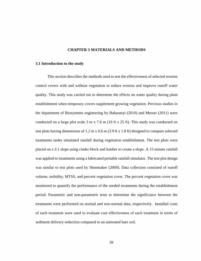
39

CHAPTER 3 MATERIALS AND METHODS

3.1 Introduction to the study

This section describes the methods used to test the effectiveness of selected erosion

control covers with and without vegetation to reduce erosion and improve runoff water

quality. This study was carried out to determine the effects on water quality during plant

establishment when temporary covers supplement growing vegetation. Previous studies in

the department of Biosystems engineering by Baharanyi (2010) and Messer (2011) were

conducted on a large plot scale 3 m x 7.6 m (10 ft x 25 ft). This study was conducted on

test plots having dimensions of 1.2 m x 0.6 m (3.9 ft x 1.8 ft) designed to compare selected

treatments under simulated rainfall during vegetation establishment. The test plots were

placed on a 3:1 slope using cinder block and lumber to create a slope. A 15 minute rainfall

was applied to treatments using a fabricated portable rainfall simulator. The test plot design

was similar to test plots used by Shoemaker (2009). Data collection consisted of runoff

volume, turbidity, MTSS, and percent vegetation cover. The percent vegetation cover was

monitored to quantify the performance of the seeded treatments during the establishment

period. Parametric and non-parametric tests to determine the significance between the

treatments were performed on normal and non-normal data, respectively. Installed costs

of each treatment were used to evaluate cost effectiveness of each treatment in terms of

sediment delivery reduction compared to an untreated bare soil.

40

3.2 Study site description and experimental set-up

The study site is located at Auburn University’s Department of Crop, Soil and

Environmental Sciences (CSES) Turfgrass Research Unit (TGRU) at 105 Shug Jordan

Parkway, Auburn, AL. A galvanized steel frame hoop house 11 m x 7.5 m (35 ft x 24 ft)

with tarps installed was used to cover the test plots, providing shelter from natural rain, and

eliminating cross winds during simulated rainfall testing. Five meters of house length was

covered with clear plastic tarps under which the seeded treatments were placed to expose

them to sunlight. The remaining 5.5 m of roofline was covered with heavy duty tarps

secured at the top and sides (Figure 3.1 and 3.2). Annual ryegrass (Lolium multiflorum)

and Browntop millet (Panicum ramosum) were used as the temporary vegetation in this

study. Pressurized water supply used for simulating rainfall was provided by a hose bib

adjacent to the plots.

Figure 3.1: Experimental installation in Auburn, AL showing placement of test plots

at 3:1 slope and placement of tarps for rain and wind protection

Test Plots

41

Figure 3.2: Experimental layout of test plots and treatments under hoop house

structure, TGRU, Auburn, AL

Note: BS (Bare soil), BS+P (Bare soil with PAM),

EFM (Engineered fiber matrix), EFM+S (EFM with seed),

WS+P (Wheat straw with PAM), WS+P+S (WS+P with seed)

Table 3.1 provides information about the test periods, along with planting and sample

dates and also the different plant species used along with their scientific names.

Table 3.1: Study period dates with plant species and planting dates

1 Data treated as preliminary to set up monitoring and sampling protocols

Growth

Period

Plant species Planting date Sample Dates

Preliminary1 Annual ryegrass

(Lolium multiflorum.)

1 Oct. 2013 21 Oct. -19 Nov. 2013

I Annual ryegrass

(Lolium multiflorum)

13 Mar. 2014 21 Mar. - 5 May 2014

II Browntop millet

(Panicum ramosum)

22 May 2014 27 May - 14 July 2014

42

3.3 Test soil analysis and composition

The soil used in the study was taken from the road banks of the forested site located

at Pittsview in Russell County, AL (32o 9’29.30”N, and 85o 10’ 8.09”W) and owned by

Alabama General Contractors Association (AGC) (Figure 3.3). Nearly 3.4 m3 (120 ft3) of

soil was excavated and transported by dump truck to the TGRU on 30 July, 2013.

Transported soil was stored under tarps until use.

The road bank location from where soil was taken is shown in Figure 3.4.

Composite samples were taken from the soil (Figure 3.5) and soil analyses were conducted

by Auburn University Soil Testing Laboratory (AUSTL) to determine soil texture and

fertilizer recommendations for grass cover.

Figure 3.3: Alabama General Contractors (AGC) site soil sample location maps,

Russell Co, AL

43

Soil fertility testing was performed twice, one before preliminary test period (17

August, 2013) and other before test period II (16 May, 2014). Soil textural analysis (Table

3.2) yielded very high sand and clay content with smaller amounts of silt. The resulting

textural class was sandy clay. The textural analysis performed before test period II yielded

the same soil texture. Soil reports recommended lime of 7.8 metric tons ha-1 (3.5 tons acre-

1) and 6.7 metric tons ha-1 (3 tons acre-1) in a soil test report before preliminary tests and

before test period II, respectively. Annual ryegrass (Lolium multiflorum) was chosen as the

seeded treatment for test period I. Annual ryegrass is a cool season annual and so that it

can be grown in early winter and spring. Browntop Millet (Panicum ramosum) was grown

in test period II in summer 2014 as warm season annual.

Table 3.2: Percent composition and textural class of experimental soil

Soil test report

date

% Sand

% Silt

% Clay

Textural Class

17 Aug., 2013 46.3 15.6 38.1 Sandy Clay

16 May, 2014 45.6 16.3 38.1 Sandy Clay

Figure 3.4: Source for

study soil: eroded road

bank, Russell County,

AL

Figure 3.5: Taking composite samples of soil for

fertility and textural analysis

44

3.4 Design and preparation of test plots

Test plots were constructed similar to Shoemaker’s (2009) test plots with pressure

treated lumber of 0.6 m (1.8 ft) width, 1.2 m (3.9 ft) length, and 0.1 m (0.46 ft) depth

(Figure 3.6) placed on a 3:1 slope using cinder blocks (Figure 3.7). Each of the test plot

bottoms were constructed from 1.3 cm (0.5 in) thick exterior grade plywood. Additional

lumber was fixed to the bottoms of selected plywood boxes for reinforcement. Drain holes

of 3.2 cm (1.3 in) diameter, were drilled at the bottom of the boxes for drainage during

simulated rainfall events. A permeable fabric was placed over the drill holes prior to soil

placement to prevent soil loss. A weir of 0.3 m (12 in) was cut into the front face of each

plot to direct water flow into fabricated flumes. Metal flumes were fabricated of sheet metal

to divert surface runoff from each test plot into collection buckets (Figure 3.8). Flumes

were fixed at the front face of each plot into the soil.

Figure 3.6: Soil filled and compacted small scale test

plots

45

Shoemaker (2009) achieved a target 95% maximum soil density using ASTM D 698

standard proctor density. McLaughlin and Brown, (2006) provided typical seedbed

preparation along a roadside to provide loose soil and match the bulk density of the soil. In

the present study, compaction was done to approximate the dry bulk density of the native

soil as a suitable seed bed. The sum of an equal number of hand tamps was used to simulate

the native seedbed and subsoil system for the vegetation establishment experiments, as

follows.

A core sample was taken from the soil site in Russell County, AL. Dry bulk density

of the soil was determined by in-situ core sampling and found out to be 0.9 g cm-3. A mold

box 25.4 cm x 25.4 cm (10 in x 10 in) was constructed and filled with native soil from the

site (Figure 3.9). Soil in the mold box was tamped several times to achieve similar dry bulk

density as the original soil. The number of hand tamps required to achieve a dry bulk

density of 0.9 g cm-3 was 60. This number of hand tamps was subsequently used to prepare

Figure 3.7: Test plots placed on 3:1 slope

using concrete blocks and lumber

Figure 3.8: Flumes to direct runoff

from test plots into collection buckets

46

each test plot. Testing and tamping of the soil was done with air dry soil. No water was

added to the soil while packing into the test plots.

Test boxes were filled using four 19 L (5 gallon) buckets to spread soil evenly to 15

cm (6 in). The soil was then compacted to 5 cm (2 in) from the top resulting in total of 10

cm (4 in) of soil in each box. The soil in each test plot was hand tamped 60 times uniformly

along the test plot (Figure 3.10) and then raked to approximately 5 cm (2 in) of loose

surface depth after compaction. Refilling of boxes before test period I and II was done by

removing the top soil, treatments and any grass grown. Two additional 19 L (5 gallon)

buckets of native soil were added, then again compacted 60 times and raked to

approximately 5 cm (2 in) of depth before the start of the new test period.

Figure 3.9: Mold box (25.4 cm x 25.4 cm) used to determine required

tamps to achieve a field bulk density of 0.9 g cm-3

47

3.5 Portable rainfall simulator

The rainfall simulator (Figure 3.11) consisted of 1.9 cm (0.75 in) galvanized steel

pipe, sprinkler nozzle, water filter, pressure regulator, pressure gauge, garden hose, and

ball valve. The sprinkler nozzle was installed 3.05 m (10 ft) above the ground to provide a

rectangular spray area of 2.4 m x 2.4 m (7.9 ft x 7.9 ft). A Single FullJet™ ½ HH – 30WSQ

spray nozzle manufactured by Spraying Systems, Co. (Wheaton, IL) was used for the

rainfall simulator. Shoemaker (2009) used the same nozzle for his study. A Senninger®

PMR-10 MF pressure regulator manufactured by Senninger Irrigation Inc., Clermont, FL

with an operating pressure of 0.69 bar (10 psi) was attached to provide a flow rate of 11.37

L min-1 (3 gpm). An Arkal® water filter with connection diameter of 1.9 cm (0.75 in)

manufactured by Arkal Filtration Systems, (Israel) was attached to the water inlet to

prevent nozzle clogging. A pressure gauge was placed after the water filter to monitor

operating pressure and a brass ball valve was used to start and end testing. A heavy duty

hose conveyed water from a pressurized water source at the site. Three test plots of each

Figure 3.10: Compaction of soil boxes (119 cm x 56 cm) by hand tamping

48

treatment were tested simultaneously. To mitigate the effects of wind during testing, the

rainfall simulator was fully enclosed in a temporary chamber made of tarps.

3.5.1 Uniformity of simulated rainfall

A uniform distribution is desirable for simulated rainfall on test plots (Hudson,

1993). Lowest distribution uniformity testing developed by USDA, NRCS was performed

to assure a uniform distribution of rainfall during testing. Both the distribution uniformity

and precipitation rate for the rainfall simulator was calculated. Twenty catch cans 30 cm

(12 in) apart were placed in five lines with each line 28 cm (11 in) apart (Figure 3.12 and

3.13). Run time for the uniformity testing was six minutes. The volume in each catch can

was recorded and the average catch of the five lowest catches (ml) was calculated.

Fulljet ™

½ HH-

30 WSQ nozzle

Figure 3.11: Portable galvanized steel rainfall simulator with sprinkler nozzle

49

Figure 3.13: Layout of catch cans on test plots to determine the lowest

distribution uniformity

Rectangular

spray area

Figure 3.12: Placement of catch cans over test plots during uniformity testing,

TGRU, Auburn, AL

50

Lowest distribution uniformity was calculated using Equation 3.1 (Duke and Perry,

2006) and determined to be 73.5% (Table 3.3), which is good for sprinkler system (The

Irrigation Association, 2002).

Where DU = Lowest distribution uniformity Ql= Avg. Catch in lowest quarter

Qt= Average catch

Table 3.3: Uniformity at six test plot locations

3.5.2 Rainfall regime

A 2-year 24-hour design depth is often used by researchers in testing of erosion

control BMPs (ASWCC, 2009) but was not feasible in this study due to the number of test

plots and resulting collection limitations. According to the manufacturer specifications, the

nozzle can produce a flow rate of 11.37 L min-1 (3 gpm) at 70 kPa (10 psi) pressure which

was verified in the field by placing 5 gallon bucket under the nozzle. As per Figure 3.13,

the spray nozzle provided a rectangular spray area 2.4 m x 2.4 m (7.9 ft x 7.9 ft). The

intensity of simulated rainfall can be calculated by using equation 3.2 (Jain Irrigation

System Ltd., India):

𝐷𝑢 = (

𝑄𝑙

𝑄𝑡) × 100

(3.1)

Test plot Uniformity

1 67.1%

2 79.1%

3 69.4%

4 75.3%

5 72.1%

6 78.3%

Average 73.5%

51

𝐼 =

60 × 𝐹

𝐴

(3.2)

Where, I = Intensity of rainfall (mm hr-1)

F = Flow rate (L min-1) = 11.37 L min-1

A = Spray Area (m2) = 2.4 m x 2.4 m

Resulting intensity was 11.84 cm h-1 and the precipitation depth based on the 15

minute rainfall runtime was 2.96 cm (1.16 in.) of rainfall. Based on City of Auburn

precipitation data for the past 36 years, the 90th percentile storm depth for 2 year-15 min

and 2 year-30 min ranges between 2.3 cm (0.9 in) to 3.3 cm (1.3 in) (NOAA, 2014).

Simulated rainfall was designed to match the rainfall depth between a 2-year 15-minute

and 2-year-30 minute storm event for the area.

3.6 Treatments

Initially, six erosion and sediment control treatments were tested in this study

including the bare soil control and bare soil with PAM and seed (BS+P+S) treatment.

However after preliminary testing, the vegetation stand failed in BS+P+S. Previous

literature indicates that PAM application is not correlated with vegetation establishment

(McLaughlin and Brown, 2006; Baharanyi, 2010). Consequently, a bare soil with PAM

and seed treatment was not included in this study. Table 3.4 summarizes the six treatments

tested with labels, trade name, manufactures, and content.

52

Table 3.4: Treatments with their trade names, manufacturers and content used in

the study

3.6.1 PAM application (Treatments: BS+P, WS+P, and WS+P+S)

EnviroPAM distributed by Innovative Turf Solutions, (Cincinnati, OH) was used

in this study. Jar testing of PAM was performed in accordance with Mississippi Department

of Environmental Quality (MDEQ, 2007) recommendations to confirm that the product

was an effective flocculant for the tested soil. A 473 ml bottle was filled with water and a

pinch of PAM was added with a teaspoon of soil. The solution was shaken for 20 seconds

and allowed to sit. The addition of PAM resulted in soil particle settlement in the jar

indicating suitability for the study soil. PAM was consequently applied uniformly to

appropriate test plots (BS+P, WS+P, WS+P+S) using a salt shaker at the manufacturer

recommended application rate of 10 kg ha-1 (9 lbs acre-1), equivalent to 0.70 g per plot.

3.6.2 Wheat straw application (Treatments: WS+P, WS+P+S)

Wheat straw is the most commonly used straw and can be applied by mechanical

mulch blower or by hand (ASWCC, 2009). Typical application of wheat straw is

accomplished by chopping and blowing straw onto the land surface to achieve

Treatment with labels Trade name Manufacturer Content

Bare soil (BS)

Bare soil with Polyacrylamide

(PAM) (BS+P)

EnviroPAM® Innovative Turf Solutions,

Cincinnati, OH

Sodium

Acrylamide

Copolymer

Engineered Fiber Matrix (EFM) Promatrix™

EFM

Profile Products, Buffalo

Groove, IL

Wood Fiber

Engineered Fiber Matrix with

seed (EFM+S)

Promatrix™

EFM

Profile Products, Buffalo

Groove, IL

Wood Fiber

Wheat straw with PAM (WS+P) EnviroPAM® Innovative Turf Solutions,

Cincinnati, OH

Wheat straw

Wheat straw with PAM and seed

(WS+P+S)

EnviroPAM® Innovative Turf Solutions,

Cincinnati, OH

Wheat straw

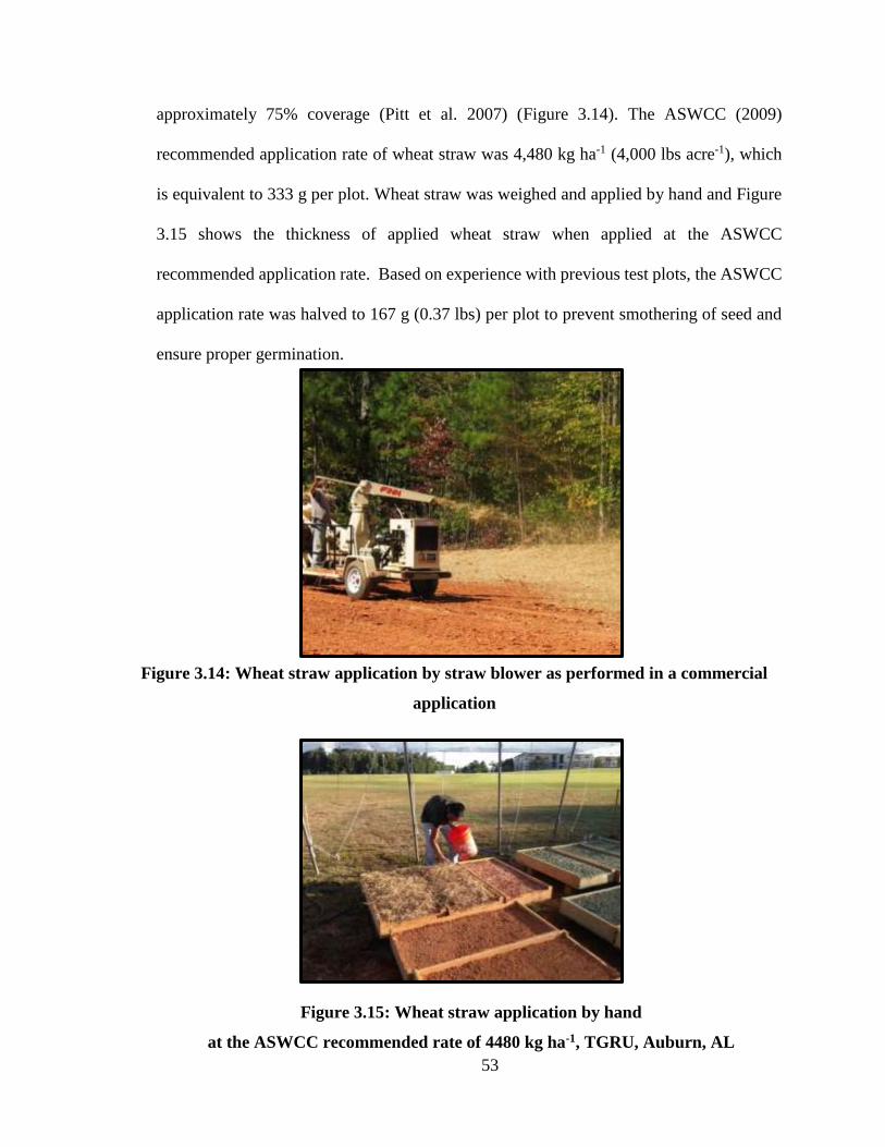
53

approximately 75% coverage (Pitt et al. 2007) (Figure 3.14). The ASWCC (2009)

recommended application rate of wheat straw was 4,480 kg ha-1 (4,000 lbs acre-1), which

is equivalent to 333 g per plot. Wheat straw was weighed and applied by hand and Figure

3.15 shows the thickness of applied wheat straw when applied at the ASWCC

recommended application rate. Based on experience with previous test plots, the ASWCC

application rate was halved to 167 g (0.37 lbs) per plot to prevent smothering of seed and

ensure proper germination.

Figure 3.15: Wheat straw application by hand

at the ASWCC recommended rate of 4480 kg ha-1, TGRU, Auburn, AL

Figure 3.14: Wheat straw application by straw blower as performed in a commercial

application

(Source: http://www.dogwoodengineering.com)

54

3.6.3 Hydraulic mulch application (EFM, EFM+S)

The hydraulic applied product tested as a temporary cover in this study was

Promatrix® EFM manufactured by Profile Products, Buffalo Grove, IL. This Product has

been approved by the Alabama Department of Transportation (ALDOT)-Product

Evaluation Board (PEB) for rolled and hydraulic erosion control products (ALDOT, 2014).

The EFM was applied using a hydromulcher system and a precision applicator, as

described below. The manufacturer’s recommended EFM application rate was 3,362 kg

ha-1 (3,000 lbs acre-1).

3.6.4 Hydromulcher/Precision applicator system

The hydromulcher used to apply the Promatrix® EFM treatment was the Turf

Maker® 380 manufactured by Turf Maker (Rowlett,TX) and shown in the Figure 3.16.

The capacity of the hydroseeder is 1,438 L (380 gallons) of hydromulch and water mixture.

In additon to a storage tank, the main components of the hydromulcher are a gasoline

powered engine, belt driven pump, and mechanical agitator.

Figure 3.16: Hydromulcher Turf Maker® 380, TGRU, Auburn, AL

55

The pressurized hyromulcher outlet was connected to a hyrdomulcher precision

applicator system developed by the Agricultural Research Station (ARS) in Lubbock, TX.

The main components of the hydromulcher system are a steel gantry, a variable frequency

drive (VFD) controller, pump/agitator, and main power disconnect (Figure 3.17). The

gantry has overall dimensions of 6.37 m x 2.43 m x 2.51 m (21 ft x 8 ft x 8.2 ft) including

electrical connections, quick connects, and spray nozzle. The VFD controller has

dimensions of 1.25 m x 0.72 m x 0.53 m (4 ft x 2.4 ft x 1.7 ft) with electric connections as

its main components. Main power to the gantry is supplied through the VFD electrical

controller. During testing, hydroseeder discharge was connected to a hose using a 3.8 cm

(1.5 in) banjo quick-connect. The hydroseeder hose and pump was connected to the gantry

hose and nozzle with a 5 cm (2 in) banjo quick-connect. A garden hose was connected to

fill the hydroseeder level above the agitator shaft to 758 L (200 gallons) along with two 23

kg (50 lbs) bags each of EFM. With the engine running, the agitator clutch was engaged to

mix the EFM and water slurry. Before each test period, the calibration was completed using

the VFD controller to set the frequency and application rate of the EFM product to be

sprayed. Calibration was based on the time the nozzle takes to cross the gantry, the inside

length and width of the box to be sprayed, and the spray height from tip of the spray nozzle

to the top of the soil inside the test box. The hydromulcher provided EFM product at

sufficient operating pressure of 1.03 bar (15 psi) to accurately apply product to test plots.

56

3.6.5 Seeded treatments (WS+P+S, EFM+S)

Soil test fertilizer recommendations for roadside turf from the Auburn University

soil testing lab were 135-179-90 kg ha-1 (120-160-80 lb. acre-1) of N, P2O5 and K2O,

respectively. Fertilizer application was calculated using available fertilizers (30-0-0 N, 0-

46-0 P and 0-0-60 K).The recommended lime application from the initial soil report was

7,845 kg ha-1 (7,000 lbs acre-1), which is equivalent to 0.58 kg (1.3 lbs.) per plot. The soil

test report before test period II indicated only that K2O was reduced by half due to high

potassium. Table 3.5 shows the fertilizer and lime recommendations for both soil test

reports.

Main power

disconnect

Spray nozzle Gantry

Figure 3.17: Components of hydromulcher precision applicator

system, TGRU, Auburn, AL (VFD controller not shown)

57

Table 3.5: Fertilizer and lime recommendation modification for test plots

Annual ryegrass and browntop millet were planted in six plots (2 treatments x 3 test

plots). In this study, grass seed was mixed with sand for uniform distribution and

incorporated into the soil by hand prior to the application of all cover treatments (WS+P

and EFM) (Figure 3.18). The recommended application rate of annual ryegrass and

browntop millet was 67 kg ha-1 (5 g per plot) and 45 kg ha-1 (3.4 g per plot), respectively.

As mentioned, soil in test plots was raked to approximately 5 cm (2 in) deep. Fertilizers

and lime were also mixed with sand in a container and applied uniformly by hand on to the

treatment surface. Hand watering was provided at a rate of 1 cm (0.39 in) every two days

after the incorporation of seed, fertilizers and lime. To ensure that seed did not runoff the

surface during hand watering, hose pressure was reduced. The data collection was started

after 7 days and 4 days of seeding in test period I and II, respectively.

Date Fertilizer

recommendations

(kg ha-1)

Fertilizer

application rate

for test plots(g)

Lime

Recommendation

(kg ha-1)

Lime

application

rate (kg)

17 Aug. 2013 135-179-80 33-29-11 7845 0.58

16 May 2014 135-179-40 33-29-5.5 6725 0.50

Figure 3.18: Application of seed by hand, TGRU, Auburn, AL

58

3.7 Data collection and analysis

Data collected for this research included (1) runoff volume (ml), (2) turbidity

(NTU), (3) MTSS (g), and (4) Percent vegetation cover. Runoff and sediment generated

from each plot during simulated rainfall was recorded as a function of time and vegetated

cover throughout the establishment period. Nineteen liter (5 gallon) buckets were fitted

under collection flumes to collect runoff from test plots. Collection buckets were covered

to ensure that no water from the simulator fell directly into the bucket (Figure 3.19).

Selected conclusions for the treatment and cost effectiveness from the data was

done according to the test period II as it has more complete set of data points than test

period I. Test periods I and II were used as a combined data set to test different grass species

in comparing seeded and non-seeded treatments. So, test period II was used in concluding

objective 1 and 3 but test periods I and II combined were used for objective 2 conclusions

(Table 3.6).

Figure 3.19: Collection of runoff from the test plots, TGRU, Auburn, AL

59

Table 3.6: Test periods used for different objective conclusions

Objectives Objective statement Conclusion basis

Objective 1 Treatment effectiveness in

water quality responses

Test period II

Objective 2 Comparison of seeded vs.

non-seeded treatment

Test period I and II

combined

Objective 3 Cost Effectiveness Test period II

3.7.1 Turbidity measurement (NTU)

Runoff was collected in each bucket until it stopped flowing from the plots. Each

runoff sample was stirred completely and an unfiltered grab sample was taken in a 150 ml

(5 oz) bottle from each test plot and brought back to the laboratory for turbidity

measurement. Turbidity was measured using a Hach 2100 P turbidimeter (Loveland, CO)

(USEPA, 2012). At the laboratory, unfiltered samples were shaken to resuspend sediments

and then poured into a 15 ml (0.5 oz) turbidimeter vial for analysis. After each sample was

analyzed, the container was rinsed with water to prevent contamination between samples.

The turbidity of bare soil plots (BS) and bare soil with PAM (BS+P) treatments routinely

exceeded the maximum reading on the turbiditimeter. As a result, samples were diluted as

needed according to manufacturing recommendations to provide in-range turbidity results

by dilution.

3.7.2 MTSS (g) & runoff volume (ml) measurement

A modified standard method for total suspended solids method (TSS 2540 D)

(USEPA 160.2) was used to determine MTSS. Modifications from the standard method

included use of filter bags in the field, rather than a filter of similar mesh with vacuum

filtration in the laboratory. After each rainfall simulation test, 1 µm filter bags (36 cm long)

60

manufactured by Hayward Flow Control (Clemmons, NC) were used to filter sediments

from collected runoff to determine modified TSS. A total of 18 bags were used per sample

date (6 treatments x 3 test plots) with each runoff sample filtered through one filter bag. To

filter runoff, filter bags were inserted into a 20 cm (8 in) PVC pipe column and the PVC

pipe was placed in a 19 L bucket (5 gallon). All collected plot runoff was poured through

the filter (Figure 3.20). Filtered runoff from each test plot was subsequently poured into a

graduated cylinder to determine the volume of runoff (Figure 3.21). Filter bags were

brought back to the laboratory and dried in a conventional forced-air oven manufactured

by VWR (Radnor, PA) at a temperature of 105o C (221o F) for a minimum of 24 hours.

The dried filter bag and soil weight was compared with oven dry weight of the bag prior to

filtration. Before and after difference of the filter bags was the dry weight of suspended

solids from each test plot, providing an estimate of sediment yield as modified TSS in each

plot.

Figure 3.20: Pouring the sediment

water into the filter bags, TGRU,

Auburn, AL

Figure 3.21: Pouring the filtered water

into graduated cylinder to measure

runoff volume, TGRU, Auburn, AL

61

3.7.3 Vegetation cover measurement

Percent vegetation cover was measured on each day of rainfall simulation and runoff

testing using the line transect method, also known as line point intercept method (Godinez-

Alvarez et al., 2009). The line transect method was performed by stretching two string

having 25 equal marks diagonally from one side of the test plot to the other (Figure 3.22).

Each point represents a sample point to be tallied when viewed from directly above. Each

plot was analyzed to determine the number of times a point hit the target grass species. The

percentage vegetation cover was determined dividing the number of hits of target grass

species (Annual ryegrass and browntop millet) by the total number of points. The two string

diagonals represent a total of 50 points per plot. Therefore, number of hits were doubled to

obtain an estimate of percent vegetation cover of the target grass.

Figure 3.22: Strings tied to test plots for vegetation cover measurement,

TGRU, Auburn, AL

62

3.8 Cost analysis

Overall performance, maintenance and required labor can affect the overall cost of

erosion control BMPs (Donald, 2013). BMP cost comparison was performed to determine

which treatment was the most cost effective per unit of sediment loss reduced. The ALDOT

maintains a cost database known as the ALDOT item bid summary, which is representative

of construction industry costs in the southeast US. Erosion control bid items listed in the

summary were classified on a cost per unit area basis (dollar per hectare). Mulching as

defined in the ALDOT bid summary includes wheat and other straws blown as a dry mulch.

The EFM treatment used in this study corresponds to type S3 ALDOT product per their

approved list II-11 dated August 5, 2013. The ALDOT bid data was divided into counties

within the state and was averaged to obtain the mean cost of erosion and sediment control

BMPs for the state of Alabama. The most current ALDOT bid summary of March 6, 2014

was used as a reference for this analysis except for PAM cost which was available only

from the ALDOT bid summary of October 1, 2012. Table 3.7 summarizes the average cost

per square meter and cost per hectare for Alabama.

Table 3.7: Average cost for selected erosion control BMPs for Alabama

1Source: ALDOT bid summary, 2012. Unit cost based on application rate of 10 kg ha-1 2 Source: ALDOT bid summary, 2014 3Straw mulching includes wheat and other straws

Treatment Average cost per sq. m. Average cost per ha

PAM1 $0.03 $307

Straw mulching2,3 $0.21 $2,062

Straw mulching with PAM2,3 $0.24 $2,369

Temporary seeding2 $0.13 $1,288

Straw mulching + PAM + seeding $0.37 $3,657

Engineered fiber matrix(EFM)2 $2.13 $21,306

EFM with seeding2 $2.26 $22,594

63

3.9 Statistical analysis

Turbidity, MTSS, runoff volume, and percent vegetation cover data recorded by

date and treatment were organized using an Excel spreadsheet. A JMP 11 software

developed by Statistical Analysis Systems (SAS) (Cary, NC) was used to determine

significant differences between the means of treatments for test periods I and II. All three

response means (runoff volume, turbidity, and MTSS) were tested separately for each test

period. Tests of normality including QQ plots were used to verify the normality of data.

Consequently, one way analysis of variance (ANOVA) was performed using general linear

model (GLM) to determine significant differences between the runoff volume means for

test periods I and II, separately. Significant differences between runoff volume means of

different treatment pairs were compared using the Tukey Kramer procedure. Significance

was reported using an alpha value (p-value) of 0.05. The typical null and alternate

hypothesis used for this research is illustrated in equations (3.3) and (3.4):

H0: µ1= µ2 =µ3 =µ4 =µ5 =µ6 (3.3)

Ha: Not all means are equal (3.4)

Where,

Ho = Null Hypothesis

Ha = alternate hypothesis

µi = Mean value of each data set ‘i’

i= independent groups (i.e. bare soil, WS + P etc.)

64

Turbidity and MTSS data were found to be non-normal and subsequently analyzed

using Kruskal Wallis Rank Sum test as an alternative non-parametric procedures. Kruskal

Wallis Rank Sum Test was used to test for the statistical differences between the means.

Kruskal Wallis test is used to test more than two groups and is an extended form of the

Mann-Whitney U test (Easton and McColl, 1997). The Kruskal Wallis uses data as ranks

instead of original values, providing p-value approximation of difference. If the K statistic

is not significant, there is no evidence of difference between the means. However, if the

test statistic is significant at least one treatments dominate at least one other treatment.

When differences were indicated, multiple comparison tests were performed to determine

the significant difference between specific pairs of all treatments means. For this series of

tests, Wilcoxon non-parametric multiple comparison tests were performed. These tests of

significant difference between pairs of treatment means were performed for turbidity and

MTSS for test periods I and II, separately. Graphical and statistical analysis of seeded

versus non-seeded treatments was analyzed using combined data from test periods I and II.

The significance between the correlated slopes of seeded and non-seeded treatments for

test periods I and II combined was determined at significance level of 0.05 using

StatGraphics software developed by Statpoint technologies, Warrenton, VA.

65

CHAPTER 4 RESULTS AND DISCUSSION

4.1 Introduction

This chapter records observed response of five erosion control covers (1) BS+P, (2)

WS, (3) WS+P, (4) EFM, and (5) EFM + S compared to the bare soil control (BS) for two

test periods. Treatment means were analyzed and results discussed in terms of benefit of

vegetated cover over time to reduce important construction runoff parameters such as

volume, turbidity and sediment. Performance ranking of the different treatments tested

were according to test period II. Graphical and statistical analysis of seeded versus non

seeded treatments was completed using combined data from test periods I and II

normalized as a function of days after seeding (DAS).

4.2 Experimental results

4.2.1 Runoff volume (ml)

Figure 4.1 illustrates runoff volume for all treatments as a function of DAS during

test period I. Bare soil has the highest mean runoff volume, as expected. In test period I,

EFM+S, EFM and WS+P+S performed similarly with an average runoff volume of 2694

ml, 2886 ml, and 4531 ml, respectively. Bare soil with PAM had the runoff volume of 9092

ml followed by WS+P with an average runoff volume of 6270 ml.

66

Figure 4.2 illustrates the runoff volume for all the cover treatments during test period

II. During test period II, EFM had the more runoff volume than during test period I due to

apparent early sealing of the soil surface by the EFM. The treatment with the most effective

volume reduction in test period II was EFM+S with an average volume of 2873 ml,

statistically similar to WS+P+S (4595 ml). EFM and WS+P were not statistically similarly

with average runoff volumes of 6265 ml and 4873 ml, respectively. All cover treatments

except BS+P reduced average runoff volumes from 30% to 68%, as compared to control

(Table 4.1).

13 17 19 26 28 36 43 520

2000

4000

6000

8000

10000

12000

Ru

no

ff v

olu

me

(m

l)

DAS

BS BS+P EFM EFM+S WS+P WS+P+S

Figure 4.1: Runoff volume for cover treatments with DAS for test period I,

Auburn, AL

67

Table 4.1 presents the mean treatment runoff volumes with standard deviation and

percent reduction, as compared to the bare soil control for both test periods. Mean runoff

ratios across test period II for the treatments are shown in the right column. The percent

runoff reduction, as compared to control in test period II was: (1) EFM+S (68%), (2)

WS+P+S (49%), (3) WS+P (46%), (4) EFM (30%), and BS+P (16%). Bare soil with PAM

used alone did not perform well in this study compared to the other covers likely due to a)

the degradation of chemical after several simulated rainfall events, b) relatively low

application rate, and c) the lack of surface roughness compared to other cover treatments.

One way ANOVA indicated significant differences between treatments in both test

periods (p-value < 0.0001). Tukey Kramer procedure indicated that neither of the EFM

treatments were significantly different in test period I, but were significantly different in

test period II due to apparent sealing in the EFM treatment, not identified in test period I.

The EFM treatment runoff volume was significantly lower than WS+P in test period I. No

statistical significance was observed between wheat straw treatments in both test periods

5 8 11 15 18 20 24 27 35 42 530

2000

4000

6000

8000

10000

12000

14000

Ru

no

ff v

olu

me

(m

l)

DAS

WS+P+S WS+P EFM+S EFM BS BS+P

Figure 4.2: Runoff volume for cover treatments with DAS for test period II,

Auburn, AL

68

indicating that vegetation seeding in wheat straw treatments did not have much effect on

average mean runoff volume. Runoff means from bare soil and bare soil with PAM

treatments were not significantly different from each other in either test period apparently

due to the low application rate of PAM. Seeded treatments (WS+P+S, EFM+S) were not

significantly different from each other in either test periods in terms of runoff volume.

Runoff volume for the EFM+S treatment was statistically lower than the EFM and WS+P

treatments indicating vegetation had a significant impact on runoff volume reduction at

least in the EFM+S treatment.

Table 4.1: Runoff volume results of all the treatments for both the test periods

Note: Treatments with same letters are not significantly different at α=0.05 1Percent reduction in runoff volume compared to control 2EFM (Engineered Fiber Matrix), EFM+S (EFM with seed), WS+P (Wheat Straw with PAM),

WS+P+S (WS+P with PAM and seed), BS+P (Bare soil with PAM), BS (Bare Soil) 3Average Runoff ratio calculated as ratio of runoff volume (ml) to precipitation applied (ml) for

test period II

Figure 4.3 shows the comparison of runoff volume of seeded and non-seeded EFM

treatments versus DAS for combined test period I and II. The graph provides information

about the effect of cover on runoff volume over time from the seeded treatments. Both the

EFM+S and EFM treatments showed a declining trend in runoff volume (r = -0.73 and -

0.42, respectively). The declining regression slopes of both treatments were not statistically

different (p value = 0.55), indicating that although test period II runoff volume mean was

Treatment2 Test Period I Test Period II Avg.

runoff

ratio3

Average vol.

(ml)

Reduction1 Average vol.

(ml)

Reduction1

BS

BS+P

EFM

EFM+S

WS+P

WS+P+S

9825±2094 a 9092±1472 a

2886±434 c

2694±294 c

6270±2452 b

4531±661 b,c

-

8%

71%

73%

36%

54%

8985±566 a

7584±1346 a,b

6265±2319 b,c

2873±690 d

4873±1400 c

4595±631 c,d

-

16%

30%

68%

46%

49%

0.42

0.35

0.29

0.13

0.23

0.21

69

significantly lower for EFM+S treatment, the relationship of rate of runoff reduction over

time was not significantly different with or without seeding.

Figure 4.4 plots runoff volume for seeded and non-seeded treatments for wheat straw

with PAM for combined test periods I and II. Seeded treatments had negative runoff

volume correlation with increased vegetation cover (r = - 0.57). Non- seeded treatment

means had rising slope and positive correlation (r = 0.62), indicating the degradation of the

non-seeded wheat straw treatment after frequent rain events similar to Wishowski et al.

(1998). Wheat straw sub sample test plots had more variable results, as compared to EFM

treatments due to varied surface contact of wheat straw. The regression slopes of both

treatments were significantly different from each other (p value < 0.0001).

Figure 4.3: Comparison of EFM seeded and non-seeded treatments with DAS

(Combined test periods I and II)

y = -40.4x + 3844.4R² = 0.54R = -0.73

y = -60.3x + 6404.3R² = 0.18R = -0.42

0

1000

2000

3000

4000

5000

6000

7000

8000

9000

0 10 20 30 40 50 60

Ru

no

ff v

olu

me

(m

l)

DAS

EFM+S I EFM I EFM+S II

EFM II Linear (EFM+S) Linear (EFM)

Slopes are not

significantly

different

(p-value =0.55)

70

4.2.2 Turbidity (NTU)

Turbidity samples grabbed from thoroughly stirred plot runoff in the catchment

buckets from each test plot were averaged by treatment. Figures 4.5(a) and (b) illustrates

the turbidity of all treatments for test period I and II versus DAS. As expected, turbidity of

the bare soil treatment (BS) was higher than any other treatment similar to the findings

reported by McLaughlin and Brown, (2006) and Wilson, (2010). In test period II, all cover

treatments except WS+P reduced turbidity below 150 NTU. EFM+S was the significantly

effective cover treatment evaluated, with an average test period II turbidity of 38 NTU

(Table 4.2). The lower value in bare soil and bare soil with PAM in test period II initially

was due to hardness and dryness of the soil but it starts rising due to the rill formation after

certain simulated rainfall events.

Figure 4.4: Comparison of runoff volume of WS+P and WS+P+S treatments with

DAS (Combined test periods I and II)

y = -61.1x + 6173.1R² = 0.33R = -0.57

y = 89.3x + 3148.5R² = 0.38R = 0.62

0

1000

2000

3000

4000

5000

6000

7000

8000

9000

10000

0 10 20 30 40 50 60

Ru

no

ff v

olu

me

(m

l)

DAS

WS+P+S I WS+P+S II WS+P I

WS+P II Linear (WS+P+S) Linear (WS+P)

Slopes are

significantly

different

(p-value< 0.0001)

71

(a) Test period I (b) Test period II

*-Data Missing in WS+P treatment

Figure 4.6 illustrate turbidity of cover treatments not including bare soil and bare soil

with PAM to more closely investigate treatment effect for test period I. In test period I,

WS+P performed well until 28 days after seeding when straw degradation becomes

prevalent. EFM, EFM+S, and WS+P+S treatments performed similarly with average

turbidity’s of 66 NTU, 84 NTU, and 134 NTU, respectively (Table 4.2). The initial

turbidity of seeded treatments in test period I was higher than non-seeded treatments likely

due to the insufficient raking of the surface in the non-seeded treatments. The EFM

treatment included a bonding agent to bond the mulch particles to soil surface. When the

bonding agent washed away after frequent storm events, the EFM treatment also starts to

lose its effectiveness as shown in both the test periods similar to the findings reported by

Wilson (2010).

Figure 4.5: Turbidity of all the cover treatments vs. DAS, Auburn, AL

72

Figure 4.7 plots test period II mean turbidity of cover treatments without BS and

BS+P. In test period II, the EFM treatment with and without seed was observed to

consistently reduce average turbidity levels to below 100 NTU. The WS+P treatment had

higher mean NTU values than any other cover treatment except BS+P treatment. EFM was

a more effective turbidity reduction treatment than wheat straw which is similar to results

reported by Babcock and McLaughlin (2013). The experimental method in test period II

was indicated by similar day 5 mean turbidity values for corresponding seeded and non-

seeded treatments. So, test period II was used for overall results due to less variability in

results, as compared to test period I.

13 17 19 26 28 36 43 520

50

100

150

200

250

300

350

400

Turb

idit

y(N

TU)

DAS

EFM EFM+S WS+P WS+P+S

Figure 4.6: Turbidity of cover treatments without BS and BS+P for test period I

73

*- Data Missing in WS+P treatment

Table 4.2 presents average turbidity values with standard deviation and percent

reduction, compared to a control for both test periods. Results were ranked from most to

least effective turbidity reduction treatments compared to the bare soil control in test period

II as: (1) EFM+S (98.7%) (2) EFM (98.3%), (3) WS+P+S (96.5%), (4) WS+P (92.4%),

and (5) BS+P (16.9%). All cover treatments except BS+P in both the test periods were able

to reduce the turbidity by over 90%, as compared to bare soil. Mean turbidity of the WS+P

treatment was higher than turbidity measured in any EFM treatment in both test periods

due to more soil exposed. No statistical significance was found between EFM, EFM+S,

and WS+P+S. The application of PAM (BS+P) were not significantly different from bare

soil (BS) in terms of turbidity reduction. However, all other test period II treatment pairs

had significantly different means from each other. The EFM+S treatment was significantly

lower than all other treatments and was the most effective treatment in terms of turbidity

reduction.

5 8 11 15 18 20 24 27 35 42 530

50

100

150

200

250

300

350

400

Turb

idit

y (N

TU)

DAS

WS+P+S WS+P EFM+S EFM

*

Figure 4.7: Turbidity of cover treatments without BS and BS+P for test period II

74

Table 4.2: Turbidity results of all the treatments for both the test periods

Note: Treatments with same letters are not significantly different at α= 0.05 1Percent reduction compared to control 2EFM (Engineered Fiber Matrix), EFM+S (EFM with seed), WS+P (Wheat Straw with PAM),

WS+P+S (WS+P with seed), BS+P (Bare soil with PAM), BS (Bare Soil)

Figure 4.8 compares turbidity means of EFM and EFM+S treatments for combined

test periods I and II. The seeded treatment (EFM+S) was observed to have declining trend

with time (r = - 0.37), as expected while the non- seeded treatment (EFM) has a flatten

response with time (r = 0.26). The slopes of both the treatments were not significantly

different from each other (p value = 0.056). Consequently, although turbidity means were

lower for EFM+S than EFM treatment, vegetation cover in EFM treatment did not have a

significant effect in turbidity reduction over time.

Treatment2 Test period I Test period II

Average turbidity

(NTU)

Percent

reduction1

Average turbidity

(NTU)

Percent

reduction1

BS

BS+P

EFM

EFM+S

WS+P

WS+P+S

2234±431 a

2120±325 a

66±25 c

84±26 c

103±46 b

134±34 b,c

-

5.1%

97.1%

96.2%

95.4%

94.0%

2946±461 a

2449±156 a

51±9 d

38±5 e

224±75 b

103±13 c

-

16.9%

98.3%

98.7%

92.4%

96.5%

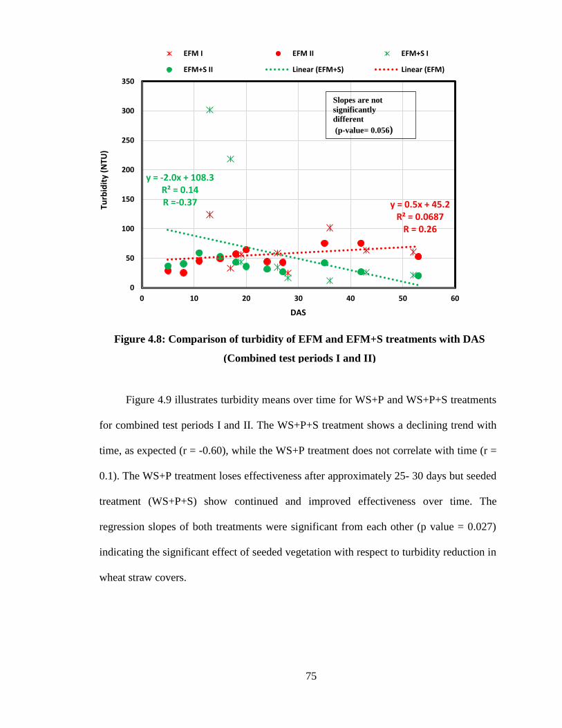
75

Figure 4.9 illustrates turbidity means over time for WS+P and WS+P+S treatments

for combined test periods I and II. The WS+P+S treatment shows a declining trend with

time, as expected (r = -0.60), while the WS+P treatment does not correlate with time (r =

0.1). The WS+P treatment loses effectiveness after approximately 25- 30 days but seeded

treatment (WS+P+S) show continued and improved effectiveness over time. The

regression slopes of both treatments were significant from each other (p value = 0.027)

indicating the significant effect of seeded vegetation with respect to turbidity reduction in

wheat straw covers.

Figure 4.8: Comparison of turbidity of EFM and EFM+S treatments with DAS


y = -2.0x + 108.3R² = 0.14R =-0.37 y = 0.5x + 45.2

R² = 0.0687R = 0.26

0

50

100

150

200

250

300

350

0 10 20 30 40 50 60

Turb

idit

y (N

TU)

DAS

EFM I EFM II EFM+S I

EFM+S II Linear (EFM+S) Linear (EFM)

Slopes are not

significantly

different

(p-value= 0.056)

76

4.2.3 MTSS for all treatments

Figures 4.10 (a) and (b) illustrate the MTSS delivered from all treatments including

the two bare soil treatments, BS and BS+P. Results indicate nearly 100 percent reduction

of sediment delivery by all cover treatments except BS+P for test period I and II. In test

period I, application of EFM+S was the most effective treatment with an average MTSS of

0.53 g similar to WS+P+S and EFM. The EFM+S with an average MTSS of 0.59 g was

significantly effective sediment reduction treatment in test period II. MTSS values on 8

April, 2014 (26 DAS) of all treatments were not reported due to data error during weighing

of the bags.

Figure 4.9: Comparison of turbidity of WS+P and WS+P+S treatments

with DAS (Combined test periods I and II)

y = -3.8x + 215.2R² = 0.36R = -0.60

y = 0.6x + 156R² = 0.01R = 0.1

0

50

100

150

200

250

300

350

400

0 10 20 30 40 50 60

Turb

idit

y (N

TU)

DAS



Slopes are

significantly

different

(p-value= 0.027)

77

(a) Test period I (b) Test Period II

Figure 4.11 illustrates MTSS excluding BS and BS+P to more closely investigate the

effects of the cover treatments for test period I. The EFM, EFM+S, and WS+P+S

treatments performed similarly with an average MTSS of 0.85 g, 0.53 g, and 1.01 g,

respectively (Table 4.3). The WS+P treatment with an average MTSS of 1.25 g performed

similar to EFM and WS+P+S treatments. High initial differences in MTSS deliveries for

wheat straw treatments was a result of unequal raking (lack of equal disturbance) in non-

seeded WS+P versus WS+P+S treatment.

Figure 4.10: MTSS of all the treatments with DAS

13 17 19 28 36 43 52

0.0

0.5

1.0

1.5

2.0

2.5

3.0

3.5

4.0

4.5

MTS

S(g)

DAS

EFM EFM+S WS+P WS+P+S

Figure 4.11: MTSS of cover treatments versus DAS without BS and BS+P

(Test period I)

78

Figure 4.12 plots mean MTSS delivered for cover treatments without BS and BS+P

versus DAS for test period II. The EFM and WS+P+S treatments performed similarly with

an average MTSS of 0.68 g and 0.97 g, respectively (Table 4.3). The WS+P treatment with

an average MTSS of 1.48 g performed equally well as the WS+P+S treatment with respect

to MTSS delivered.

Table 4.3 presents the average MTSS delivered for all treatments with standard

deviations and percent reduction compared to the bare soil control. In test period II, the

effectiveness of treatments were ranked from the most effective to least effective as: (1)

EFM+S (99.8%) (2) EFM (99.7%) (3) WS+P+S (99.6%) (4) WS+P (99.4%) (5) BS+P

(22.6%). Doolette and Smyle (1990), in a review of 200 studies, reported that mulch

reduced soil erosion between 78 to 98 percent. In test period I, EFM+S had significantly

lower MTSS delivery than WS+P, but it was not significantly different from EFM and

WS+P+S. The sediment delivery of WS+P treatment was not significantly different from

5 8 11 15 18 20 24 27 35 42 53

0

0.5

1

1.5

2

2.5

MTS

S (g

)

DAS

WS+P+S WS+P EFM+S EFM

Figure 4.12: MTSS delivery of cover treatments versus DAS without BS and

BS+P

(Test period II)

79

EFM (Babcock, 2008; Lee, 2012) and WS+P+S in test period I. In test period II, the MTSS

of the EFM+S treatment was significantly lower than all other cover treatments indicating

the overall effect of vegetation in EFM treatments for sediment reduction. EFM sediment

delivery was also observed to be significantly lower than WS+P likely due to the variable

surface contact of wheat straw. Wheat straw treatment means were not significantly

different from each other in both test periods indicating that seeded vegetation in wheat

straw doesn’t provide a significant effect on average MTSS delivered. The sediment

delivery of BS and BS+P treatment were not significantly different from each other in both

test periods due to relatively low application rate of PAM used in the study.

Table 4.3: Results of MTSS (g) of all the treatments for both the test periods

Note: Treatments with same letters are not significantly different at α=0.05 1Percent reduction compared to control 2EFM (Engineered Fiber Matrix), EFM+S (EFM with seed), WS+P (Wheat Straw with PAM)

WS+P+S (WS with PAM and seed), BS+P (Bare soil with PAM), BS (Bare Soil)

Figure 4.13 compares average MTSS delivery of EFM and EFM+S treatments for

combined test periods I and II. The observed declining trend in seeded treatment (EFM+S)

MTSS with time (r = -0.61) was expected, while non- seeded treatments had a flat response

with time (r = 0.03), as expected. The non-seeded EFM treatment (EFM) performed

consistently over the time period, as expected. The slopes of both the treatments were not

significantly different from each other (p value = 0.07). So, while vegetation has a

Treatments2 Test Period I Test Period II

Average MTSS

(g)

Percent

reduction1

Average MTSS

(g)

Percent

reduction1

BS

BS+P

EFM

EFM+S

WS+P

WS+P+S

351±73 a

313±126 a

0.85±0.33 c,b

0.53±0.19 c

1.25±0.30 b

1.01±0.26 c,b

-

10.8%

99.8%

99.9%

99.6%

99.7%

235±27 a

182±21 a

0.68±0.36 c

0.59±0.30 d

1.48±0.90 b

0.97±0.28 c,b

-

22.6%

99.7%

99.8%

99.4%

99.6%

80

significant impact on the magnitude of sediment reduction during the establishment period,

the impact of seeding over time was not verified statistically at the alpha value tested (α =

0.05).

Figure 4.14 represents the MTSS delivery means of WS+P and WS+P+S treatments

with DAS for combined test periods I and II. WS+P+S performed better in terms of MTSS

reduction than in runoff volume and turbidity reduction. The declining trend in the seeded

wheat straw treatment (r = -0.71) as compared to a flat response in the non-seeded wheat

straw treatment (r = 0.2) indicates the importance of vegetation for sediment delivery

reduction in a wheat straw treatment. After approximately 30 days, The MTSS of the

WS+P treatment began to increase due to loss of treatment effectiveness. The slopes of

seeded versus non-seeded treatment were significantly different from each other (p value

= 0.045). Therefore, vegetation was observed to have a significant impact in MTSS

Figure 4.13: Comparison of MTSS of EFM and EFM+S treatments with DAS


y = -0.03x + 1.2R² = 0.37R = -0.61

y = -0.0012x + 0.7R² = 0.0009

R = 0.03

0

0.5

1

1.5

2

2.5

0 10 20 30 40 50 60

MTS

S (g

)

DAS

EFM+S I EFM+S II EFM I

EFM II Linear (EFM+S) Linear (EFM)

Slopes are not

significantly

different

(p-value= 0.07)

81

reduction in wheat straw treatment over time. So, a seeded wheat straw treatment

(WS+P+S) would be a better option, as compared to a non-seeded treatments for long term

(> 30 days) sediment delivery reduction.

4.3 Percent vegetation cover with time

Percent vegetation cover was measured and recorded using the line-point intercept

method. The percent vegetation cover versus DAS is presented in Figure 4.15 (a) and (b)

for EFM+S and WS+P+S, respectively, for combined test periods I and II. The highest

value of percent vegetation cover was 90% and 64% in WS+P+S treatment in test periods

I and II, respectively. Similarly, McLaughlin and Brown (2006) reported higher vegetation

cover in straw than measured in a BFM treatment. The EFM with seed treatment in the

present study resulted in a maximum vegetation cover of 75% and 70% in test periods I

Figure 4.14: Comparison of MTSS of WS+P and WS+P+S treatments with DAS


y = -0.05x + 2.3R² = 0.51R = -0.71 y = 0.0033x + 1.3

R² = 0.005R = 0.2

0

0.5

1

1.5

2

2.5

3

3.5

4

4.5

0 10 20 30 40 50 60

MTS

S (g

)

DAS



Slopes are

significantly

different

(p-value= 0.045)

82

and II, respectively. Higher R-square and postive slope indicates consistent growth of

vegetation cover over time in seeded treatments in this study.

(a) % veg. cover of EFM+S versus DAS (b) % Veg cover of WS+P+S versus DAS

4.4 Cover factor

The cover factor is a parameter used in the Revised Universal Soil Loss Equation

(RUSLE) to represent the cover condition compared to an unprotected bare soil (Clopper

et al., 2001). The RUSLE cover factor characterizes the effect of surface cover and

roughness on soil erosion. The cover factor is calculated as the ratio of sediment yield of a

given cover or surface condition to the sediment yield of an unprotected bare soil condition.

Cover factor is the most common factor used to test the effectiveness of BMPs for erosion

reduction (Renard et al., 1997). Table 4.4 summarizes the estimated cover factor for test

periods I and II separately for all the treatments normalized to a bare soil (BS) control. The

value of all cover factors lies between 0 and 1 in which 0 means the treatment resulted in

100% reduction of erosion and 1 means that the treatment is equivalent to bare soil

Figure 4.15: Percent vegetation cover of seeded treatments versus DAS


y = 1.4x + 1.8R² = 0.93R = 0.96

0

10

20

30

40

50

60

70

80

90

100

0 10 20 30 40 50 60%

ve

g co

ver

DAS

WS+P+S I WS+P+S II

Linear (WS+P+S)

y = 1.3x + 4.8R² = 0.97R = 0.98

0

10

20

30

40

50

60

70

80

90

100

0 10 20 30 40 50 60

% v

eg

cove

r

DAS

EFM+S I EFM+S II

Linear (EFM+S)

83

conditions and did not result in any reduction of erosion. Table 4.4 shows the ranking of

treatments in test period II from most to least effective with respect to cover factor as: (1)

EFM+S (0.0025) (2) EFM (0.0029) (3) WS+P+S (0.0041) (4) WS+P (0.0063) (5) BS+P

(0.7747).

Table 4.4: Cover factor for all the treatments

1Cumulative MTSS from test period I 2C factor normalized to bare soil value of 2453 g/plot for test period I 3Cumulative MTSS from test period II 4C factor normalized to bare soil value of 2579 g/plot for test period II 5EFM (Engineered Fiber Matrix), EFM+S (EFM with seed), WS+P (Wheat Straw with PAM)

WS+P+S (WS with PAM and seed), BS+P (Bare soil with PAM)

4.5 Percent vegetation cover combined effect

Figure 4.16 shows the response of seeded treatments for both test periods versus

percent vegetation cover indicating a declining trend in runoff volume with increased

percent vegetation cover (r = -0.49), as expected in this study. Some of the values are higher

initially in test period I due to non-uniformity of the raked surface for the non-seeded

surface. In general, all seeded treatments values decreased with increased percent

vegetation cover. This graphical representation also shows the impact of growing

vegetation on runoff volume over the course of the study period. Numerous studies report

similar runoff reduction with increase in percent vegetation cover (Adekalu et al., 2007;

Foltz and Copeland, 2009).

Treatment5 Test period I Test period II

MTSS

(grams/plot)1

cover factor (C)2 MTSS

(grams/plot)3

cover factor (C)4

EFM+S 3.71 0.0015 6.52 0.0025

EFM 5.99 0.0024 7.43 0.0029

WS+P+S 7.07 0.0029 10.61 0.0041

WS+P 8.77 0.0036 16.24 0.0063

BS+P 2188.00 0.8920 1998.00 0.7747

84

Figure 4.17 illustrates the effect of percent vegetation cover on turbidity over the

study period. The correlation coefficient (r = -0.47) indicates a turbidity reduction with

increased percent vegetation cover, as expected.

Figure 4.16: Effect of percent vegetation cover on runoff volume of seeded

treatments (Combined test periods I and II)

Figure 4.17: Effect of percent vegetation cover on turbidity of seeded treatments


y = -37.9x + 5131.5R² = 0.24R = -0.49

0

1000

2000

3000

4000

5000

6000

7000

8000

9000

0 10 20 30 40 50 60 70 80 90

Ru

no

ff v

olu

me

(m

l)

% veg cover

Seeded I Seeded II Linear (Seeded treatments)

y = -2.1x + 167.4R² = 0.22R = -0.47

0

50

100

150

200

250

300

350

400

0 10 20 30 40 50 60 70 80 90

Turb

idit

y (N

TU)

% veg cover


85

Figure 4.18 shows the effect of increased vegetation cover on MTSS for seeded

treatments during combined test periods I and II. The correlation of percent vegetation with

MTSS reduction was higher (r = -0.63), as compared to runoff volume and turbidity.

Similar sediment yield reductions were confirmed by other researchers with increased

percent vegetation cover (Liu et al., 2010; Pan and Shangguan, 2006).

4.6 Comparison of seeded and non-seeded treatments

Additional analysis was performed on the response data to compare all seeded

versus all non-seeded treatments, as a function of DAS. Since not all treatments received

seeding, differences can be evaluated based on equal time period after seeding dates.

Regression and correlation patterns for runoff volume, turbidity and MTSS delivered

indicate a response from seeded treatments over non-seeded treatments and provide

Figure 4.18: Effect of percent vegetation cover on MTSS of seeded treatments


y = -0.03x + 1.8R² = 0.40R = -0.63

0

0.5

1

1.5

2

2.5

3

3.5

4

4.5

0 10 20 30 40 50 60 70 80 90

MTS

S (g

)

% veg cover


86

evidence across independent time periods of the water quality benefits of seeding in

conjunction with other temporary covers, irrespective of species.

Runoff volume

Figure 4.19 indicates that the runoff volume of all seeded treatments for test period I

and II combined correlate negatively (r = - 0.48), as compared to the flat response of non-

seeded treatments (r = 0.10) with DAS. The vegetation intercept the rainfall falling on it,

which results in low runoff volume. The slopes of data sets were significantly different

from each other (p-value = 0.025), confirming the impact of vegetation over time, as

compared to non-seeded treatments.

Figure 4.19: Comparison of runoff volume of seeded and non-seeded treatments with


y = 14.5x + 4776.4R² = 0.01R = 0.10

y = -51.2x + 5008.7R² = 0.23R = -0.48

0

1000

2000

3000

4000

5000

6000

7000

8000

9000

10000

0 10 20 30 40 50 60

Ru

no

ff v

olu

me

(m

l)

DAS

Seeded I Non-Seeded I

Non-Seeded II Seeded II

Linear (Non-Seeded treatments) Linear (Seeded treatments)

Slopes are significantly

different (p-value= 0.025)

87

Turbidity

Figure 4.20 plots mean turbidity of seeded and non-seeded treatments over time for

test periods I and II combined. The correlation between seeded treatments and DAS (r = -

0.47) was higher than non-seeded treatments (r = 0.01). Root structure of the vegetation

have strengthen the soil and keeping the sediment on its place. The slopes of both the

treatments were significantly different (p-value = 0.016) indicating the impact of seeded

vegetation on turbidity reduction over time.

MTSS

Figure 4.21 illustrates MTSS treatment means for both test periods of seeded and

non-seeded treatments versus DAS. Seeded treatments have the highest correlation (r = -

Figure 4.20: Comparison of turbidity of seeded and non- seeded treatments

with DAS (Combined test periods I and II)

y = 14.5x + 4776.4R² = 0.0099

R = 0.01

y = -2.9x + 161.7R² = 0.22R = -0.47

0

50

100

150

200

250

300

350

400

0 10 20 30 40 50 60

Turb

idit

y (N

TU)

DAS

Seeded I Non-Seeded I

Non-Seeded II Seeded II

Linear (Non-seeded treatments) Linear (Seeded treatments)

Slopes are significant

at α= 0.05

(p-value= 0.016)

88

0.63) of all study responses. Non-seeded treatments showed consistent performance over

time (r = 0.02), as expected. The vegetation helps restrict the sediment movement from one

place to another, thus reducing the soil loss. The slope of seeded treatments was

significantly lower than the slope of non-seeded treatments (p-value = 0.0016). So,

vegetation was helpful for continued stabilization of disturbed slopes, as compared to non-

.seeded treatments.

4.7 Cost benefit analysis

ArcMap by Environmental Systems and Research Institute (ESRI®), Redlands, CA

was used to create maps of BMP cost per square meter by county for each product evaluated

in this study. Plots are presented as Figures 4.22 to 4.26.

Figure 4.21: Comparison of MTSS of seeded and non-seeded treatments vs


y = 0.001x + 1.0R² = 0.0005

R = 0.02

y = -0.04x + 1.7R² = 0.40R = -0.63

0

0.5

1

1.5

2

2.5

3

3.5

4

4.5

0 10 20 30 40 50 60

MTS

S (g

)

DAS

Seeded I Non-seeded I

Non-seeded II Seeded II

Linear (Non-seeded treatments) Linear (Seeded treatments)

Slopes are significant

at α= 0.05

(p-value= 0.0016)

89

\

$ 0 – Data not available

Figure 4.22: Unit cost of seeding per sq. mt. for ALDOT projects

(ALDOT, 2014)

Sumter$0.00 Dallas

$0.05

Lee$0.15

DeKalb$0.00

Colbert$0.00

Marengo

$0.11

Cleburne$0.13

Greene$0.00

Bibb$0.18

Cherokee$0.12

Dale$0.08

Pickens$0.19

Escambia$0.00

Choctaw$0.00

Clarke$0.15

Marshall$0.13

Coffee$0.00

Barbour$0.01

Tallapoosa

$0.15

Lamar$0.00

Wilcox$0.07

Coosa

Butler$0.03

Geneva $0.01

Limestone$0.00

Franklin$0.15

Randolph

$0.20

Fayette

$0.40

Henry

$0.02

Monroe$0.13

St.Clair$0.16

Russell$0.14

Walker$0.12

Hale

Mobile$0.19

Blount$0.14

Winston$0.00

Montgomery

$0.11

Elmore$0.01

Lauderdale $0.15

Clay

$0.19

Morgan

$0.11

Jackson$0.00

Chambers$0.14

Cullman$0.15

Chilton$0.00

Lawrence$0.15

Calhoun$0.22

Crenshaw$0.00

Conecuh$0.00

Etowah$0.19

Perry

$0.00

Bullock$0.01

Marion$0.25

Tuscaloosa$0.22

Shelby

$0.15

Pike$0.03

Washington

$0.00 Covington

$0.08

Madison$0.14

Lowndes$0.07

Autauga

$0.10

Baldwin$0.16

Macon$0.05

Jefferson$0.17

Temp seed

±

0 40 80 120 16020Kilometers

Legend

AL

Temp_Seed

$0.00

$0.01 - $0.25

$0.26 - $0.40

90


Figure 4.23: Unit cost of EFM per sq. mt. for ALDOT projects

(ALDOT, 2014)

Sumter$0.00

Dallas

Lee$1.75

DeKalb$0.00

Colbert$0.00

Marengo

$0.00

Cleburne$1.72

Greene$0.00

Bibb$0.00

Cherokee$0.00

Dale$0.00

Pickens$0.00

Escambia$0.00

Choctaw$2.06

Clarke$1.77

Marshall$0.00

Coffee$0.00

Barbour$0.00

Tallapoosa

$0.00

Lamar$2.34

Wilcox$2.62

Coosa$0.00

Butler$0.00

Geneva $0.00

Limestone$0.00

Franklin$0.00

Randolph

$0.00

Fayette

$0.00

Henry

$0.00

Monroe$0.00

St.Clair$2.12

Russell$1.51

Walker$5.37

Hale$0.00

Mobile$1.44

Blount$1.81

Winston$0.00

Montgomery

$1.89

Elmore$0.00

Lauderdale $0.00

Clay

$0.00

Morgan

$0.00

Jackson$0.00

Chambers$0.00

Cullman$2.33

Chilton$0.00

Lawrence$3.17

Calhoun$0.00

Crenshaw$0.00

Conecuh$2.01

Etowah$2.06

Perry

$0.00

Bullock$1.99

Marion$1.45

Tuscaloosa$0.00

Shelby

$1.82

Pike$0.00

Washington

$0.00 Covington

$0.00

Madison$1.70

Lowndes$0.00

Autauga

$2.83

Baldwin$1.89

Macon$1.77

Jefferson$1.75

EFM per sq mt

±

0 40 80 120 16020Kilometers

Legend

AL

EFM

0.00

0.01 - 3.17

3.18 - 5.37

91


Figure 4.24: Unit cost of EFM+S per sq. mt. for ALDOT projects

(ALDOT, 2014)

Sumter$0.00 Dallas

$0.00

Lee$1.90

DeKalb$0.00

Colbert$0.00

Marengo

$0.00

Cleburne$1.85

Greene$0.00

Bibb$0.00

Cherokee$0.00

Dale$0.00

Pickens$0.00

Escambia$0.00

Choctaw$0.00

Clarke$1.92

Marshall$0.00

Coffee$0.00

Barbour$0.00

Tallapoosa

$0.00

Lamar$0.00

Wilcox$2.69

Coosa

Butler$0.00

Geneva $0.00

Limestone$0.00

Franklin$0.00

Randolph

$0.00

Fayette

$0.00

Henry

$0.00

Monroe$0.00

St.Clair$2.28

Russell$1.65

Walker$5.49

Hale

Mobile$1.63

Blount$0.00

Winston$0.00

Montgomery

$2.00

Elmore$0.00

Lauderdale $0.00

Clay

$0.00

Morgan

$0.00

Jackson$0.00

Chambers$0.00

Cullman$2.48

Chilton$0.00

Lawrence$3.32

Calhoun$0.00

Crenshaw$0.00

Conecuh$0.00

Etowah$2.25

Perry

$0.00

Bullock$2.00

Marion$1.70

Tuscaloosa$0.00

Shelby

$1.97

Pike$0.00

Washington

$0.00 Covington

$0.00

Madison$1.84

Lowndes$0.00

Autauga

$2.93

Baldwin$2.05

Macon$1.82

Jefferson$1.92

EFM+TS

±

0 40 80 120 16020Kilometers

Legend

AL

EFM+TS

$0.00

$0.01 - $3.32

$3.33 - $5.49

92


Figure 4.25: Unit cost of mulching per sq. mt. for ALDOT projects

(ALDOT, 2014)

Sumter$0.33 Dallas

$0.19

Lee$0.19

DeKalb$0.23

Colbert$0.18

Marengo

$0.19

Cleburne$0.16

Greene$0.21

Bibb$0.19

Cherokee$0.18

Dale$0.21

Pickens$0.33

Escambia$0.16

Choctaw$0.19

Clarke$0.16

Marshall$0.33

Coffee$0.13

Barbour$0.08

Tallapoosa

$0.26

Lamar$0.25

Wilcox$0.14

Coosa$0.00

Butler$0.17

Geneva $0.15

Limestone$0.00

Franklin$0.24

Randolph

$0.00

Fayette

$0.00

Henry

$0.14

Monroe$0.16

St.Clair$0.19

Russell$0.27

Walker$0.21

Hale$0.00

Mobile$0.17

Blount$0.18

Winston$0.18

Montgomery

$0.14

Elmore$0.09

Lauderdale $0.19

Clay

$0.34

Morgan

$0.23

Jackson$0.17

Chambers$0.21

Cullman$0.23

Chilton$0.40

Lawrence$0.24

Calhoun$0.22

Crenshaw$0.28

Conecuh$0.17

Etowah$0.20

Perry

$0.37

Bullock$0.09

Marion$0.29

Tuscaloosa$0.28

Shelby

$0.24

Pike$0.12

Washington

$0.16 Covington

$0.16

Madison$0.21

Lowndes$0.14

Autauga

$0.25

Baldwin$0.18

Macon$0.15

Jefferson$0.24

Mulching per sq mt

±

0 40 80 120 16020Kilometers

Legend

AL

Mulching

0.00

0.01 - 0.23

0.24 - 0.40

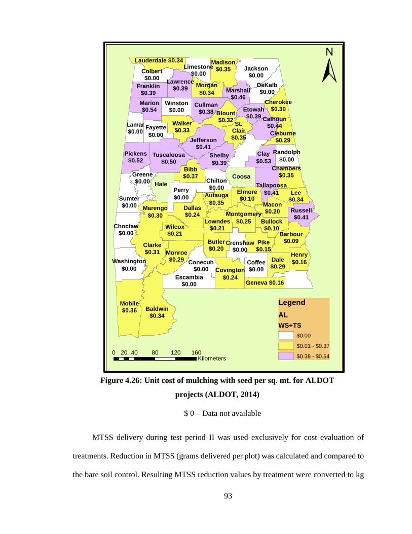
93


MTSS delivery during test period II was used exclusively for cost evaluation of

treatments. Reduction in MTSS (grams delivered per plot) was calculated and compared to

the bare soil control. Resulting MTSS reduction values by treatment were converted to kg

Figure 4.26: Unit cost of mulching with seed per sq. mt. for ALDOT

projects (ALDOT, 2014)

Sumter$0.00 Dallas

$0.24

Lee$0.34

DeKalb$0.00

Colbert$0.00

Marengo

$0.30

Cleburne$0.29

Greene$0.00

Bibb$0.37

Cherokee$0.30

Dale$0.29

Pickens$0.52

Escambia$0.00

Choctaw$0.00

Clarke$0.31

Marshall$0.46

Coffee$0.00

Barbour$0.09

Tallapoosa

$0.41

Lamar$0.00

Wilcox$0.21

Coosa

Butler$0.20

Geneva $0.16

Limestone$0.00

Franklin$0.39

Randolph

$0.00

Fayette

$0.00

Henry

$0.16

Monroe$0.29

St.Clair$0.35

Russell$0.41

Walker$0.33

Hale

Mobile$0.36

Blount$0.32

Winston$0.00

Montgomery

$0.25

Elmore$0.10

Lauderdale $0.34

Clay

$0.53

Morgan

$0.34

Jackson$0.00

Chambers$0.35

Cullman$0.38

Chilton$0.00

Lawrence$0.39

Calhoun$0.44

Crenshaw$0.00

Conecuh$0.00

Etowah$0.39

Perry

$0.00

Bullock$0.10

Marion$0.54

Tuscaloosa$0.50

Shelby

$0.39

Pike$0.15

Washington

$0.00 Covington

$0.24

Madison$0.35

Lowndes$0.21

Autauga

$0.35

Baldwin$0.34

Macon$0.20

Jefferson$0.41

EFM+TS

±

0 40 80 120 16020Kilometers

Legend

AL

WS+TS

$0.00

$0.01 - $0.37

$0.38 - $0.54

94

ha-1. The cost of each treatment derived from the ALDOT bid item summary in $ per ha

(Table 4.5) was divided by kg ha-1 MTSS reduction values (Table 4.5) to determine the

dollar spent per kg of MTSS reduction. Tables 4.5 presents the resulting cost analysis for

all temporary seeded and non-seeded cover treatments analyzed in this study. Results

indicate that BS+P was the most cost-effective treatment with $0.38 spent for each kg of

sediment reduced compared to the bare soil. However, as BS+P was not significantly

different from a bare soil control in terms of total sediment delivery reduction, BS+P is not

considered beneficial as a water quality protection BMP, at least at the application rates

used in this study (10 kg ha-1). WS+P, the next most cost effective treatment ($0.67 kg-1)

can be recommended where quick inexpensive cover is needed for slope stabilization, but

regular disturbance with 30 days does not justify the cost of seeding. EFM treatment ($6.00

kg-1), which was more expensive than the wheat straw treatments, can be applied for the

slopes adjacent to the sensitive streams requiring quick stabilization to prevent water

quality degradation.

Vegetation provides a practical long term solution for slope stabilization and erosion

control on disturbed sites (Pitt et al., 2007). Seeded treatments in this study (WS+P+S,

EFM+S) were compared to recommend a roadside slope stabilization option for similar

study site conditions. Because neither of the seeded treatments (WS+P+S and EFM+S)

were significantly different from each other in terms of percent cover establishment (Figure

4.15), differences in MTSS delivery were used to quantify the most beneficial BMP in

terms of cost and water quality benefits from erosion reduction. The EFM+S treatment

delivered 39% less MTSS per ha than WS+P+S (Table 4.5) however WS+P+S (cost of

$3,657 ha-1) was approximately 84% less expensive than EFM+S (cost of $22,594 ha-1).

95

Consequently, unless there is a special need or site consideration for hydro-applied product,

EFM+S does not appear as economical when nearly the same performance can be achieved

with WS+P+S. Therefore, WS+P+S can be considered as cost effective option compared

to EFM+S in terms of water quality protection by reduced sediment delivery under similar

slopes, soil, and rainfall conditions for the small scale test conditions.

Table 4.5: Average cost comparison by mean treatment MTSS

1MTSS for test period II 2ALDOT bid summary, 2014 3Bare soil 4Bare soil with PAM 5Wheat straw with PAM 6Wheat straw with PAM and seed 7 Engineered fiber matrix 8 Engineered fiber matrix with seed 9 MTSS reduction compared to the bare soil control 10ALDOT bid summary, 2012

BS3 BS+P4 WS+P5 WS+P+S6 EFM7 EFM+S8

MTSS/plot (g)1 235 182 1.48 0.97 0.68 0.59

MTSS/ha (g) 3,560,606 2,757,576 22,424 14,697 10,303 8,939 MTSS reduction

(g/ha)9 0 803,030 3,538,182 3,545,909 3,550,303 3,551,667 MTSS reduction

(kg/ha)9 0 803 3,538 3,546 3,550 3,552 Cost /ha2 NA $30710 $2,369 $3,657 $21,306 $22,594 Dollar/sediment

reduction ($/kg) $0.38 $0.67 $1.03 $6.00 $6.36

Inexpensive Expensive

96

CHAPTER 5 SUMMARY AND FUTURE RECOMMENDATIONS

5.1 Summary and conclusions

The main objective of the study was to test the erosion control performance of

selected erosion control covers (EFM, EFM+S, WS+P, WS+P+S and BS+P) compared to

the bare soil (BS) control in terms of water quality response (runoff volume, turbidity and

MTSS delivery) under simulated rainfall. The most cost effective treatment was

determined for roadside and similar construction sites under conditions similar to this

study. Test plots of 1.2 m x 0.6 m were constructed of pressure treated lumber and placed

on 3:1 slope under shelter. The soil in each test plot was compacted to approximate the in-

situ dry bulk density (0.9 g cm-3) of the native soil. Soil test and manufacturer’s

recommendations for fertilizer, lime, seed, and PAM application rate were converted to

equivalent test plot scales for each. Seed was incorporated into the soil before cover

placement. Wheat straw was applied at one half of the recommended application rate to

ensure seed germination. EFM treatments were applied using a Turf Maker® 380 (Rowlett,

TX) hydromulcher and USDA-ARS precision applicator. Data was gathered from two test

periods using annual ryegrass (Lolium multiflorum) and browntop millet (Panicum

ramosum), respectively, in seeded treatments.

Runoff was generated using a rainfall simulator run for 15 minutes on three replicates

of each treatment. Runoff was collected in buckets through metal flumes with runoff

samples taken to the laboratory for turbidity measurement. Runoff samples filtered in the

97

field through 1 µm filter bags were subsequently dried in the laboratory for 24 hours to

determine MTSS. Filtered water volume measured in the field provided a measure of total

runoff volume from each plot. Percent vegetation cover data was collected throughout the

study on runoff sample dates using the line-point intercept method. Cost per ha data for

each treatment was assembled from ALDOT bid summaries and used to determine the most

cost effective treatment in terms of MTSS reduction compared to bare soil.

The first objective of the study was to compare runoff volume, turbidity, and MTSS

response of each treatment to determine the water quality benefits of each. Test period II

data was used for ranking treatments in terms of water quality response as it provided a

more complete set of data points than test period I. Ranked runoff volume reduction in

treatments compared to control was: (1) EFM+S (68%), (2) WS+P+S (49%), (3) WS+P

(46%), (4) EFM (30%), and (5) BS+P (16%). Runoff volume of the EFM+S treatment was

significantly lower than WS+P, EFM, BS+P, and BS treatments. Runoff volume of EFM+S

and WS+P+S treatments were not significantly different from each other. Ranked turbidity

reduction in treatments compared to control was: (1) EFM+S (98.7%) (2) EFM (98.3%),

(3) WS+P+S (96.5%), (4) WS+P (92.4%), and (5) BS+P (16.9%). The turbidity of the

EFM+S treatment was significantly lower than the other treatments. All cover treatments

except BS+P reduced sediment delivery by over 99%, as compared to control with the

following rankings: (1) EFM+S (99.8%) (2) EFM (99.7%) (3) WS+P+S (99.6%) (4) WS+P

(99.4%) (5) BS+P (22.6%). A cover factor was calculated for all cover treatments with

ranked results from most to least effective are as follows: (1) EFM+S (0.0025), (2) EFM

(0.0029), (3) WS+P+S (0.0041), (4) WS+P (0.0063), and (5) BS+P (0.7747).

98

The second objective of this study was to quantify the beneficial impact of seeded

treatments compared to non-seeded treatments in terms of runoff, turbidity, and MTSS

response. Water quality response of the WS+P+S treatment was negatively correlated with

DAS with respect to runoff volume (r = -0.57), turbidity (r = -0.60), and MTSS (r = -0.71).

Compared to the non-seeded WS+P treatment, WS+P+S significantly reduced mean

turbidity only. Consequently, the seeded WS+P+S treatment had a significant effect on

turbidity but not much effect on runoff volume or MTSS reduction, as compared to WS+P.

Water quality response of seeded treatments combined (EFM+S and WS+P+S) were

negatively correlated with DAS with respect to runoff volume (r = -0.48), turbidity (r =-

0.47), and MTSS (r = -0.63). There was a flat correlation of corresponding responses with

DAS in non-seeded treatments (r = 0.10, 0.01, and 0.02, respectively), documenting the

important water quality benefit of seeding as an erosion control practice.

The third objective of the study was to evaluate the cost effectiveness of temporary

covers in terms of sediment delivery reduction and offer recommendations based on water

quality and budget requirements. Average cost of treatments derived from ALDOT bid

summaries were used to determine the most cost effective treatment in this study. Cost

effectiveness was defined in terms of MTSS sediment delivery reduction compared to the

bare soil control. The most cost effective treatment was BS+P, with a cost of $0.38 kg-1

sediment reduction compared to the control. However, since mass load reduction in BS+P

was not observed to be significantly different from the bare soil control, the BS+P treatment

at test rates used in this study (10 kg ha-1) was not recommended. The EFM treatment (cost

$6.00 kg-1 sediment reduction) at almost 16 times the normalized cost of BS+P is widely

used as a temporary cover for slopes adjacent to sensitive areas because of its documented

99

performance. Although EFM+S (cost $6.36 kg-1 sediment reduction) was significantly

more effective than WS+P+S in terms of MTSS sediment reduction (39% less MTSS

delivered), EFM+S was 84% more expensive. Therefore, in this study WS+P+S (cost $1.03

kg-1 sediment reduction) provided good water quality protection benefits and was

considered the most economical of the treatments tested. Consequently, the seeded

WS+P+S treatment can be recommended as a cost effective sediment delivery reduction

option for roadside slopes under conditions similar to this small scale study.

5.2 Future recommendations

The following future work can be performed to provide further data to reduce erosion

and sedimentation while providing long term slope stability.

1. This study focused on the short period of vegetation establishment for erosion

and sediment reduction. Future studies should also focus on longer vegetation

establishment periods.

2. Higher application rates of PAM, along with more than one application to

minimize chemical degradation can be a future research focus.

3. Cover treatments need to be tested under natural rainfall and field scale

conditions to better assess effectiveness under more realistic conditions.

4. Different species of vegetation can be evaluated to test the effect of species

on runoff water quality response.

5. Wheat straw with lower than recommended application rates may leave some

soil exposed, so application rates can be adjusted and evaluated with seed to

quantify runoff water quality benefits and long term slope stabilization

success.

100

6. Evaluate treatments with sodded turf for applications where immediate cover

is required for maximum protection or stringent water quality requirements.

7. RUSLE cover factors can be estimated for any treatment on a weekly or daily

basis for potential RUSLE II modelling.

101

REFERENCES

Note: References are according to the ASABE guidelines

Adekalu, K., I. Olorunfemi, and J. Osunbitan. 2007. Grass mulching effect on infiltration,

surface runoff, and soil loss of three agricultural soils in Nigeria. Bioresource Tech.

98(4): 912-917.

Ageyi, Y. 2004. Optimum Use of Erosion Control Blankets and Waste Ballast (Rock)

Mulch to Aid Grass Establishment on Steep Slopes. Journal of Hydrological

engineering. 9(2): 150-159.

Akbarzadeh, A., R. Mehrjardi, H. Refahi, H. Rouhipour, and M. Gorji. 2009. Using soil

binders to control runoff and soil loss in steep slopes under simulated rainfall. Int.

Agrophysics. 23: 99-109.

Alabama Department of Transportation (ALDOT). 2014. Rolled and hydraulic erosion

control products. Available at:

http://www.dot.state.al.us/mtweb/Testing/MSDSAR/doc/QMSD/Lii11.pdf.

Accessed on: 13 November 2014.

Arnaez, J., V. Laarea, and L. Ortigosa. 2004. Surface runoff and soil erosion on unpaved

forest roads from rainfall simulation tests in northeastern Spain. Catena. 57(1): 1-

14.

Arnaez, J., T. Lasanta, P. Ruiz-Flano, and L. Ortigosa. 2007. Factors affecting runoff and

erosion under simulated rainfall in Mediterranean vineyards. Soil Tillage Res. 93:

324-334.

Alabama Soil and Water Conservation Committee (ASWCC). 2009. Alabama handbook

for erosion control, sediment control, and storm water management on

construction site and urban areas. Available at:

http://swcc.alabama.gov/pages/erosion_handbook.aspx. Accessed on: 8

November 2014.

Babcock, D., and R. McLaughlin. 2008. Soil Facts: Mulch options for erosion control on

construction sites. Available at: http://content.ces.ncsu.edu/20431.pdf. Accessed

on: 4 November 2014.

http://www.dot.state.al.us/mtweb/Testing/MSDSAR/doc/QMSD/Lii11.pdf

http://swcc.alabama.gov/pages/erosion_handbook.aspx

http://content.ces.ncsu.edu/20431.pdf

102

Babcock, D., and R. McLaughlin. 2011. Runoff water quality and vegetative establishment

for groundcovers on steep slopes. Journal of Soil and Water Conservation. 66 (2):

132-141

Babcock, D., and R. McLaughlin. 2013. Erosion control effectiveness of straw,

hydromulch and polyacrylamide in a rainfall simulator. Journal of Soil and Water

Conservation.68 (3): 221-227.

Baharanyi, A. 2010. Techniques for establishing vegetation for erosion control on

disturbed slopes in Alabama. MS thesis, Auburn University, Auburn, AL.

Balls, P., S. Hull, B. Miller, J. Pirie and W.Proctor. 1997. Trace metal in Scottish estuarine

and coastal sediments. Marine Pollution Bulletin. 34: 42–50.

Barrett, M., L. Irish, J. Malina, and R. Charbeneau. 1998. Characterization of highway

runoff in Austin, Texas area. J. Environ. Eng. 124(2): 131–137.

Benik, S., B.Wilson, D. Biesboer, and B. Hansen. 2003. Performance of erosion control

products on a highway embankment. Transactions of the ASAE 46(4): 1113–1119.

Berndtsson, J.C. 2010. Green roof performance towards management of runoff water

quantity and quality: a review. J. Ecological Engineering. 36(4): 351-360.

Bjorneberg, D., J. Aase and D. Westermann. 2000. Controlling sprinkler irrigation runoff,

erosion, and phosphorus loss with straw and polyacrylamide. Transactions of the

ASAE. 43(6): 1545-1551.

Boardman, J. 2001. Storms, floods and soil erosion on the South Downs, East Sussex,

autumn and Winter 2000 – 01. Geography. 86 (4): 346 – 355.

Bochet, E., and P. Garcia Fayos. 2004. Factors controlling vegetation establishment and

water erosion on motorway slopes in Valencia, Spain. Restoration Ecology. 12(2):

166-174.

Bochet, E., P. Garcia Fayos and J. Tormo. 2010. How can we control erosion of roadslopes

in semiarid Mediterranean areas? Soil improvement and native plant establishment.

Land Degradation Development. 21(2): 110-121.

Booth, D., S. Cox, T. Meikle and C. Fitzgerald. 2006. The accuracy of ground-cover

measurements. Rangeland ecology & management.59 (2): 179-188.

Bradley, E., M. Barrett, A. McFarland, and L. Hauck. 2010. Hydrologic and water quality

aspects of using a compost/mulch blend for erosion control. Journal of Irrigation

and Drainage Engineering. 136(9): 646-655.

103

Broz, B., D. Pfost, and A.Thompson. 2003. Controlling runoff and erosion at urban

construction sites. Available at:

https://mospace.umsystem.edu/xmlui/bitstream/handle/10355/9480/ControllingRu

noffErosion.pdf?sequence=3. Accessed on 10 November 2014.

Bruces, W. R., L. F. Vandam, R. G. Bell, M. O. Green, and J. P. Kim. 1996. Heavy metal

and suspended sediment fluxes from a contaminated, intertidal inlet (Manukau

Harbour, New Zealand). Marine Pollution Bulletin, 32: 812–822

Cerda, A. 2007. Soil water erosion on road embankments in eastern Spain. Sci. Total

Environment. 378(1): 151-155.

Cerda, A., S. Ibanez, and A. Calvo. 1997. Design and operation of small and portable

rainfall simulator for rugged terrain. Soil techonology. 11(2): 163-170.

Chen, Y., R.C. Viadero Jr., X. Wei, R. Fortney, L.B. Hedrick, S.A. Welsh, J.T. Anderson

and L. S. Lin. 2009. Effects of highway construction on stream water quality and

macroinvertebrate condition in a mid-Atlantic highlands watershed, USA. J.

Environ. Qual. 38: 1672–1682.

Christine, K. 2014. Turbidity, Total suspended solids and water clarity. Available at:

http://www.fondriest.com/environmental-measurements/parameters/water-

quality/turbidity-total-suspended-solids-water-clarity/. Accessed on: 12 November

2014.

Clopper, P.E., M. Vielleux, and T. Johnson. 2001. Quantifying the performance of hillslope

erosion control best management practices: In Proc. ASCE EWRI Conf.-Bridging

the Gap: Meeting the World’s Water and Environmental Resources Challenges. 1-

10. Orlando, FL.

Cornelis, W.M., G. Erpul, and D. Gabriels. 2004. The I.C.E. wind tunnel for wind and

water interaction research. In Wind and rain interaction in erosion, 195-224.

Wageningin, Netherlands. ESW publication.

Damian, S. 1988. Development sediment quality criteria. Environmental Science and

Technology. 22(11): 1256-1261.

Davis, A. P., M. Shokouhian, and S. Ni. 2001. Loading estimates of lead, copper, cadmium,

and zinc in urban runoff from specific sources. Chemosphere. 44(5): 997–1009.

Dogwood Engineering. 2013. Civil engineering and design blogs. Available at:

http://dogwoodengineering.com/site- work-complete/ Accessed 26 May 2014.

Donald, W. 2013. Performance evaluations on ditch check practices and products for

channelized stormwater runoff control using large-scale testing. Ph. D.

Dissertation. Department of Civil Engg. Auburn University. Auburn, AL.

https://mospace.umsystem.edu/xmlui/bitstream/handle/10355/9480/ControllingRunoffErosion.pdf?sequence=3

https://mospace.umsystem.edu/xmlui/bitstream/handle/10355/9480/ControllingRunoffErosion.pdf?sequence=3

http://www.fondriest.com/environmental-measurements/parameters/water-quality/turbidity-total-suspended-solids-water-clarity/

http://www.fondriest.com/environmental-measurements/parameters/water-quality/turbidity-total-suspended-solids-water-clarity/

http://dogwoodengineering.com/site-%20work-complete/

104

Doolette, J.B., and J.W. Smyle. 1990. Soil and moisture conservation technologies: review

of literature. Watershed developments in Asia: Strategies and technologies. World

book technical paper no. 127. Washington, D.C.

Dougherty, M., A. Baharanyi, E. Guertal, W. Zech, C. LeBleu, and E. Norton. 2008.

Evaluation of erosion and sediment control cover types for long term vegetation

establishment on disturbed slopes. ASABE Paper No. 085300. St. Joseph, Mich.:

ASAE.

Dougherty, M., A. Baharanyi, E. Guertal, J. Grace, W. Zech, C. LeBleu, and E. Norton.

2010. Techniques for establishing vegetation for long-term erosion control on

disturbed slopes in Alabama. In Proc. Environmental connection 10, proceedings

of conference 41, 1-12. Dallas, TX.

Duke, M., and C. Perry. 2006. Uniformity testing of variable-rate center pivot irrigation

control systems. Precision Agriculture. 7(3): 205-218.

Durango Herald. 2013. Stopping erosion in its tracks. Available at:

http://durangoherald.com/article/20130731/NEWS06/130739908/Stopping-

erosion-in-its-tracks#/storyimage/DU/20130731/NEWS06/130739908/AR/0/AR-

130739908.jpg&maxw=620&maxh=400. Accessed on: 31 October 2014.

Easton, V., and J. McColl. 1997. Statistics Glossary. Available at:

http://www.stats.gla.ac.uk/steps/glossary/nonparametric.html. Accessed on: 24

November 2014.

Enriquez, A., M. J. Carrasco, and J. M. Varela. 2004. Monitoring the effectiveness of plant

restoration of the slopes of the highways. Civil. 134: 27–35.

Esteves, M., O. Planchon, J. M. Lapetite, N. Silvera and P. Cadet. 2000. The ‘EMIRE’

large rainfall simulator: design and field testing. Earth Surface Processes and

Landforms.25: 681-690.

Etchberger, C., and P. R. Krausman. 1997. Evaluation of five methods for measuring

desert vegetation. Wildlife Society Bulletin. 25(3): 604-609.

Faucette, L. B., L. M. Risse, M. A Nearing, J. W. Gaskin, and L. T. West. 2004. Runoff,

erosion, and nutrient losses from compost and mulch blankets under simulated

rainfall. Journal of Soil and Water Conservation. 59(4): 154-160.

Faucette, L.B., J. Governo, R. Tyler, G. Gigley, C.F. Jordan, and B.G. Lockaby. 2009.

Performance of compost filter socks and conventional sediment control barriers

used for perimeter control on construction sites. Journal of soil and water

conservations. 64(1): 81-88.

Ferrara, R. A. 1986. Toxic Pollutants: Impact and Fate in Receiving Waters. Urban Runoff

Pollution. 10: 423–435

http://durangoherald.com/article/20130731/NEWS06/130739908/Stopping-erosion-in-its-tracks#/storyimage/DU/20130731/NEWS06/130739908/AR/0/AR-130739908.jpg&maxw=620&maxh=400



http://www.stats.gla.ac.uk/steps/glossary/nonparametric.html

105

Flanagan, D.C., and K. Chaudhari. 1999. Erosion Control with polyacrylamide on steep

slopes. ASABE Paper No. 99. St. Joseph, Mich.: ASAE.

Flanagan D.C., K. Chaudhari, and L.D. Norton. 2002a. Polyacrylamide soil amendment

effects on runoff and sediment yield on steep slopes: part I. simulated rainfall

conditions. Transactions of the ASAE. 45(5): 1327-1337.

Flanagan, D.C., K. Chaudhari, and L.D. Norton. 2002b. Polyacrylamide soil amendment

effects on runoff and sediment yield on steep slopes: part II. Natural rainfall

conditions. Transactions of the ASAE. 45(5): 1339-1351.

Flanagan, D. C., and N. H. Canady. 2006. Use of polyacrylamide in simulated land

application of lagoon effluent: Part I. runoff and sediment loss. Transactions of the

ASABE. 49(5): 1361−1369

Foltz, R.B., and J.H. Dooley. 2003. Comparison of erosion reduction between wood strands

and agricultural straw. Transactions of the ASAE. 46(5): 1389-1396.

Foltz, R. B., and N. S. Copeland. 2009. Evaluating the efficacy of wood shreds for

mitigating erosion. J. Environ. Mgmt. 90(2): 779-785.

Foster, G.R., D.K. Mccool, K.G. Renard and W.C. Moldenhauer. 1981. Conversion of the

universal soil-loss equation to SI-units. J. Soil Water Conservation. 36: 355-359

Foster Supply. 2012. HydraCX2® hydromulch. Available at:

http://www.fostersupply.com/Products/Erosioncontrol/HydraCX2Hydromulch.as

px. Accessed on 31 October 2014.

Fox, J., S. Bhattarai, and Y. Gyasi- Agyei. 2010. Evaluation of different seed mixtures for

grass establishment to mitigate soil on steep slopes of railway batters. Journal of

irrigation and drainage engineering.137 (9): 624-631.

Freebairn, D. M., and S.C. Gupta. 1990. Microrelief, rainfall and cover effects on

infiltration. Journal of Soil and Tillage Research. 16: 307-327.

Gabriel, A. 2009. Do engineers and contractors have a choice for slope erosion control?

Available at:

http://www.ieca.org/membersonly/cms/content/Proceedings/Object450PDFEnglis

h.pdf. Accessed on: 20 October 2014

Gautier, C.R. 1983. Sedimentation in burned watersheds: is emergency revegetation

justified? Water Resources Bulletin. 19: 793-802.

Gjessing, E., E. Lygren, L. Berglind, T. Gulbrandsenm, and R. Skaane. 1984. Effects of

highway runoff on lake water quality. Sci. Tot. Environ. 33: 245–257

http://www.fostersupply.com/Products/Erosioncontrol/HydraCX2Hydromulch.aspx

http://www.fostersupply.com/Products/Erosioncontrol/HydraCX2Hydromulch.aspx

http://www.ieca.org/membersonly/cms/content/Proceedings/Object450PDFEnglish.pdf.

http://www.ieca.org/membersonly/cms/content/Proceedings/Object450PDFEnglish.pdf.

106

Godinez-Alvarez, H., J. E. Herrick, M. Mattocks, D. Toledo, and J. V. Zee. 2009.

Comparison of three vegetation monitoring methods: Their relative utility for

ecological assessment and monitoring. Ecological Indicators. 9: 1001-1008

Grace, J.M. 2000. Forest road sideslopes and soil conservation techniques. Journal of Soil

and water conservation.55 (1): 96-101.

Grace, J.M. 2002. Effectiveness of vegetation in erosion control from forest road

sideslopes. Transaction of the ASABE. 45(3): 681-685.

Green, V.S., D.E. Stott, L.D. Norton, and J.G. Graveel. 2000. Polyacrylamide molecular

weight and charge effects on infiltration under simulated rainfall. Soil Science

Society of America. 64(5): 1786-1791

Greene, R. B., P. A. Kinnell, and J. T. Wood. 1994. Role of plant cover and stock trampling

on runoff and soil erosion from semi-arid wooded rangelands. Australian Journal

of Soil Research .32: 953-973.

Grierson, I.T., and J. M. Oades. 1977. A rainfall simulator for field studies of runoff and

erosion. J. Agric.Enggg. 22: 37-44.

Groen, H., and S. W. Woods. 2008. Effectiveness of aerial seeding and straw mulch for

reducing post-wildfire erosion, north-western Montana, USA. International

Journal of Wildland Fire. 17(5): 559–571.

Gross, C.M., J.S. Angel, R.L.Hill, and M.S.Welterlen. 1991. Runoff and sediment losses

from tall fescue under simulated rainfall. Journal of Environmental quality. 20(3):

604-607.

Gyssels, G., J. Poesen, E. Bochet, and Y. Li. 2005. Impact of plant roots on the resistance

of soils to erosion by water: a review. Prog. Phys. Geogr. 29: 189–217.

Hayes, S.A., R.A. McLaughlin, and D.L. Osmond. 2005. Polyacrylamide use for erosion

and turbidity control on construction sites. Journal of Soil and Water

Conservation.60 (4): 193-199.

He, W., I. Wallinder, and C. Leygraf. 2001. A laboratory study of copper and zinc runoff

during first flush and steady-state conditions. Corros. Sci. 43(1): 127–146.

Holt, G.A., M. Buser, D. Harmel; K. Potter, and M. Pelletier .2005.Comparison of cotton-

based hydro-mulches and conventional wood and paper hydro-mulches-study. The

Journal of Cotton Science. 9: 121-127.

Hubbert, K.R. 2004. Treatment effectiveness monitoring for southern California

wildfires: 2003 to 2004. Available at:

http://www.fs.fed.us/psw/publications/4403/BAEREffectivenessMonitoringSoCA

.pdf. Accessed on: 3 November 2014.

http://www.jswconline.org/search?author1=S.A.+Hayes&sortspec=date&submit=Submit

http://www.jswconline.org/search?author1=R.A.+McLaughlin&sortspec=date&submit=Submit

http://www.jswconline.org/search?author1=D.L.+Osmond&sortspec=date&submit=Submit

http://www.fs.fed.us/psw/publications/4403/BAEREffectivenessMonitoringSoCA.pdf

http://www.fs.fed.us/psw/publications/4403/BAEREffectivenessMonitoringSoCA.pdf

107

Hudson, N. 1993. Field measurement of soil erosion and runoff. 68th edition. Food and

Agricultural organization of United Nations.

Idaho BMP manual. 2014. EC-12: Vegetation/ Seeding. Available at:

http://itd.idaho.gov/enviro/stormwater/BMP/PDF%20Files%20for%20BMP/Chap

ter%201/EC-12%20Vegetation-Seeding.pdf. Accessed on 8 September 2014.

Jain Irrigation Systems. 2014. Design data. Available at:

http://jainpipe.com/Designtechnical/data.htm. Accessed on 20 October 2014.

Jennings, S.B., N.D. Brown, and D. Sheil. 1999. Assessing forest canopies and understorey

illumination: canopy closure, canopy cover and other measures. Forestry. 72(1):

59–74.

Jiang, L., I. Dami, H.M. Mathers, W.A. Dick, and D. Doohan. 2011. The effect of straw

mulch on simulated simazine leaching and runoff. Weed Sci. 59: 580–586.

Jin, G., and A.J. Englande Jr. 2009. A field study on cost-effectiveness of five erosion

control measures. Management of Environmental Quality: An International

Journal. 20(1): 6 – 20.

Jordan Lopez, A., L. Martinez Zavala, and N. Bellinfante. 2009. Impact of different parts

of unpaved forest roads on runoff and sediment yield in a Mediterranean area. Sci

Total Environ. 407(2): 937-944.

Kaspar, T.C., J. K. Radke, and J. M. Laflen. 2001. Small grain cover crops and wheel traffic

effects on infiltration, runoff and erosion. J. Soil Water Conserv. 56: 160–164.

Kay, B. L. 1980. Mulch choices for erosion control and plant establishment. Weeds Trees

Turf. 19 (8): 16-24.

Kukal, S.S., and M. Sarkar. 2010. Splash erosion and infiltration in relation to mulching

and polyvinyl alcohol application in semi-arid tropics. Arch. Agron. Soil Sci. 56:

697–705.

Lado, M., and M. Ben-Hur. 2004. Soil mineralogy effects on seal formation, runoff and

soil loss. Applied Clay Science. 24: 241–250.

Lal, R. 2004. Soil carbon sequestration impacts on global climate change and food security.

Science. 304 (5677): 1623–1627.

Lal, R. 1998. Soil erosion impact on agronomic productivity and environment quality.

Critical Reviews in Plant Sciences. 17: 319–464.

http://itd.idaho.gov/enviro/stormwater/BMP/PDF%20Files%20for%20BMP/Chapter%201/EC-12%20Vegetation-Seeding.pdf

http://itd.idaho.gov/enviro/stormwater/BMP/PDF%20Files%20for%20BMP/Chapter%201/EC-12%20Vegetation-Seeding.pdf

http://jainpipe.com/Designtechnical/data.htm

108

Lan, J., W. Qi, P. Yue, and L. LeJing. 2012. Application of soil erosion modulus and

universal soil loss equation in assessment of environment impact-taking example

for Taizhou ecological tourism area of Jiangsu province. Acta Agriculturae Jiangxi.

24(2): 147-149.

Lancaster, T., and D.N. Austin. 2004. Classifying rolled erosion control products: a current

perspective. Land and water magazine. 48(4): 27-33.

Landloch. 2002. Studies of hydromulch effectiveness. National Centre for Engineering in

Agriculture Publication 1000455/1, USQ, Toowoomba. Available at:

http://www.cograss.com/HydromulchResearch.pdf. Accessed on: 3 November

2014.

Lee, F., and A. Jones-Lee. 1994. Are real water quality problems being addressed by

current structural best management practices. Public Works.126 (1): 54-56.

Lee, J. H., and K. W. Bang. 2000. Characterization of urban stormwater runoff. Water Res.

34(6): 1773–1780.

Lee, S.S., C.J. Gantzer, A.L. Thompson, and S.H. Anderson. 2011. Polyacrylamide

efficacy for reducing soil erosion and runoff as influenced by slope. Journal Soil

Water Conservation 66(3): 172-177.

Lemly, A. D. 1982. Erosion control at construction sites on red clay soils. Environmental

Management.6 (4): 343-352.

Lentz, R. D., and D. L. Bjorneberg. 2003. Polyacrylamide and straw residue effects on

irrigation furrow erosion and infiltration. Journal of Soil and Water Conservation.

58(5): 312-318.

Li, Y., X. Q. Xu, and X. M. Zhu. 1992a. Preliminary study on mechanism of plant roots to

increase the anti-scouribility on the Loess Plateau. Sci. China Series B- Chemistry.

35(9): 1085-1092.

Li, Y., X. Q. Xu, and X. M. Zhu. 1992b. Effectiveness of plant roots on increase the soil

permeability on the Loess Plateau. Chinese Sci. Bull. 37(20): 1735-1738.

Li, R. Y., H. Yang, J. Chen, T. Y. Yu, F. Yu. 2006. Distribution and pollution evaluation

of heavy metals in sediments of Lake Dianchi in the estuary of the Panlongjiang

River. Soils. 38(2): 186–191.

Lipscomb, C.M., T. Johnson, R. Nelson, and T. Lancaster. 2006. Comparison of erosion

control technologies: blown straw vs. erosion control blankets. Available at:

http://www.americanexcelsior.com/erosioncontrol/library/Technical%20Papers/Bl

own%20Straw%20vs.%20Erosion%20Control%20Blankets.pdf. Accessed on: 4

November 2014.

http://www.cograss.com/HydromulchResearch.pdf

http://www.americanexcelsior.com/erosioncontrol/library/Technical%20Papers/Blown%20Straw%20vs.%20Erosion%20Control%20Blankets.pdf

http://www.americanexcelsior.com/erosioncontrol/library/Technical%20Papers/Blown%20Straw%20vs.%20Erosion%20Control%20Blankets.pdf

109

Liu, G., F. X. Tian, D. N. Warrington, S. Q. Zheng, and Q. Zhang. 2010. Efficacy of grass

for mitigating runoff and erosion from an artificial loessial earthen road. American

Society of Agricultural and Biological Engineers.53(1): 119-125.

Malik, R. K., T.H. Green, G.F. Brown, and D. Mays. 2000. Use of cover crops in short

rotation hardwood plantations to control erosion. Biomass and Bioenergy .18(6):

479-487.

Marchand, C., E. Lallier-Verges, F. Baltzer, P. Alberica, D. Cossac, and P. Baillif. 2006.

Heavy metals distribution in mangrove sediments along the mobile coastline of

French Guiana. Marine Chemistry. 98: 1–17.

Marques, M. J., R. Bienes, L. Jimenez, and R. Perez-Rodriguez. 2007. Effect of vegetal

cover on runoff and soil erosion under light intensity events. Rainfall simulation

over USLE plots. Science of the Total Environment. 378: 161-165.

Martinez, M., R. Abadia, C. Sanchez, V. Manuel, and A. Juan. 2001. Experimental design

with a rainfall simulator to study the erosion changes within storm. Revista C & G.

15(1-2): 31-43.

McLaughlin, R. A. 2006. Soil Facts: Using polyacrylamide (PAM) to reduce erosion on

construction sites. North Carolina Extension Service. Available at:

http://www.soil.ncsu.edu/publications/Soilfacts/agw439-61_low-res-060106.pdf.

Accessed on 17 October 2014.

McLaughlin, R. A., and T. T. Brown. 2006. Evaluation of erosion control products with

and without added polyacrylamide. Journal of the American Water Resources

Association. 42(3): 675-684.

Mississippi Department of Environmental Quality (MDEQ) .2007. Erosion control,

sediment control and stormwater management on construction sites and urban

areas. Available at:

http://opcgis.deq.state.ms.us/Erosion_Stormwater_Manual_2ndEd/Volume1/Chap

_4_Sections/4_6/V1_Chap4_6_Sediment_Control_FLC.pdf. Accessed 26 May

2014.

Meerkerk, A. 2008. Rainfed orchards in semi-arid environments: retaining the water and

the soil. Ph.D. diss. University College London.

Megahan, W.F., K.A. Seyedbagheri, and P.C. Dodson. 1983. Long-term erosion on granitic

roadcuts based on exposed tree roots. Earth Surf Processes Landf. 8(1): 19-28.

Megahan, W. F., S. B. Monsen, M. D. Wilson, N. Lozano, D. F. Haber, and G. D. Booth.

2006. Erosion control practices applied to granitic roadfills for forest roads in

Idaho: Cost effectiveness evaluation. Land degradation and development.3 (1): 55-

65.

http://www.soil.ncsu.edu/publications/Soilfacts/agw439-61_low-res-060106.pdf

http://opcgis.deq.state.ms.us/Erosion_Stormwater_Manual_2ndEd/Volume1/Chap_4_Sections/4_6/V1_Chap4_6_Sediment_Control_FLC.pdf

http://opcgis.deq.state.ms.us/Erosion_Stormwater_Manual_2ndEd/Volume1/Chap_4_Sections/4_6/V1_Chap4_6_Sediment_Control_FLC.pdf

110

Messers, C. 2011. Evaluating maintenance techniques for long-term vegetation

establishment on disturbed slopes in Alabama. MS thesis, Auburn University,

Auburn, AL.

Miller, W.P. 1987. A solenoid-operated, variable intensity rainfall simulator. Journal of

Soil Sci. Society of America. 51: 832-834.

Mitchell, D.J., A.P. Barton, M.A. Fullen, T. J. Hocking, W. Zhi, and Z.Yi. 2003. Field

studies of the effects of jute geotextiles on runoff and erosion in Shropshire, UK.

Soil Use and Management. 19: 182-184

Montoro, J.A., J.A. Rogel, J. Querejeta, E. Diaz, and V. Castillo. 2000. Three hydro

seeding revegetation techniques for soil erosion control on anthropic steep slopes.

Land Degradation & Development.11: 315–325.

Morgan, R.C., and M.A. Nearing. 2011. Handbook of erosion modelling. 1st ed.: Blackwell

Publishing Ltd. United Kingdom.

Munn, J. R. 1974. Development and use of a portable rainfall simulator to determine the

erosion characteristics of several soils in the Lake Tahoe Basin. MS thesis,

University of California at Davis.

Muzzi, E., F. Roffi, M. Sirotti, and U. Bagnaresi. 1997. Revegetation techniques on clay

soil slopes in northern Italy. Land Degradation & Development. 8: 127–137.

Navas, A. 1993. Soil losses under simulated rainfall in semi-arid shrublands of the Erbo

Valley, Spain. Journal of Soil Use and Management. 9: 152-157.

NOAA. 2014. Hydrometerological design studies center, PFDS. Available at:

http://hdsc.nws.noaa.gov/hdsc/pfds/pfds_map_cont.html?bkmrk=al. Accessed on

20 October 2014.

Novotny, V. 1991. Urban diffuse pollution: Sources and abatement. Water Environ.

Technol. 3: 60–65.

Novotny, V., and H. Olem. 1994. Water quality prevention, identification and management

of diffuse pollution. Van Nostrand Reinhold, New York.

Novotny, V. 2003. Water quality: Diffuse pollution and watershed management. John

Wiley & Sons. NY.

Ouyang, D., and J. Bartholic. 2001. Web-Based GIS Application for Soil Erosion

Prediction. In Proc. An International Symposium - Soil Erosion Research for the

21st Century, 260-263. Honolulu, HI.

http://hdsc.nws.noaa.gov/hdsc/pfds/pfds_map_cont.html?bkmrk=al

111

Pan, C., and Z. Shangguan. 2006. Runoff hydraulic characteristics and sediment generation

in sloped grassplots under simulated rainfall conditions. Journal of Hydrology.331

(1): 178-185.

Partington, M., and G. Mehuys. 2005. Effectiveness of polyacrylamide in reducing soil

erosion on steep slopes. ASABE Paper No. 052052. St. Joseph, Mich.: ASAE.

Pekey, H. 2006. The distribution and sources of heavy metals in Izmit Bay surface

sediments affected by a polluted stream. Marine Pollution Bulletin. 52: 1197–1208

Peterson, J.R., D.C. Flanagan, and J. K. Tishmack. 2002. PAM application methods and

electrolyte source effects on plot scale runoff and erosion. Transactions of the

American Society of Agricultural Engineers. 45(6):1859-1867.

Pimentel, D., C. Harvey, P. Resosudarmo, K. Sinclair, D. Kurz, M. McNair, S. Crist, L.

Shpritz, L. Fitton, R. Saffouri, and R. Blair. 1995. Environmental and economic

costs of soil erosion and conservation benefits. Science. 267: 1117-1123.

Pitt, R., E. Clark, and W. Lake. 2007. Construction Site Erosion and Sediment Controls:

Planning, Design and Performance. Lancaster, PA: DES tech Publications, Inc.

Prats, S., M. Malvar, D. Vieira, L. MacDonald, and J. Keizer. 2013. Effectiveness of

hydromulching to reduce runoff and erosion in a recently burnt pine plantation in

central Portugal. Land Degradation and Development. Available at:

http://dx.doi.org/10.1002/ldr.2236 . Accessed on 20 November 2014.

Renard, K. G., G. R. Foster, G. A. Weesies, D. K. McCool, and D. C. Yoder. 1997.

Predicting soil erosion by water: a guide to conservation planning with the revised

universal soil loss equation. Available at:

http://www.ars.usda.gov/SP2UserFiles/Place/64080530/RUSLE/AH_703.pdf.


Roa-Espinosa, A., G.D. Bubenzer, and E.S. Miyashita, 1999. Sediment and runoff control

on construction sites using four application methods of polyacrylamide mix.

ASABE Paper No.99. St. Joseph, Mich.: ASAE.

Robichaud, P. R., J. L. Beyers, and D. G. Neary. 2000. Evaluating the effectiveness of

postfire rehabilitation treatments. General Technical Report RMRS-GTR-63.

USDA Forest Service, Rocky Mountain Research Station. Fort Collins, Colorado.

Roth, C. H., B. Meyer, and H.G. Frede. 1985. A portable rainfall simulator for studying

factors affecting runoff, infiltration and soil loss. Catena. 12 (1): 79–85.

Ruthven, D.C. III, C. Donald, E. Timothy, L. Samuel, and C. Eric. 1993. Long-term effects

of root plowing on vegetation in the eastern south Texas plains. J. Range mgt.46

(4): 351-354.

http://www.engineeringvillage.com.spot.lib.auburn.edu/controller/servlet/Controller?CID=quickSearchCitationFormat&searchWord1=%7bPeterson%2C+J.R.%7d&section1=AU&database=1&yearselect=yearrange&sort=yr

http://www.engineeringvillage.com.spot.lib.auburn.edu/controller/servlet/Controller?CID=quickSearchCitationFormat&searchWord1=%7bFlanagan%2C+D.C.%7d&section1=AU&database=1&yearselect=yearrange&sort=yr

http://www.engineeringvillage.com.spot.lib.auburn.edu/controller/servlet/Controller?CID=quickSearchCitationFormat&searchWord1=%7bTishmack%2C+J.K.%7d&section1=AU&database=1&yearselect=yearrange&sort=yr

http://dx.doi.org/10.1002/ldr.2236

http://www.ars.usda.gov/SP2UserFiles/Place/64080530/RUSLE/AH_703.pdf

http://www.sciencedirect.com/science/article/pii/S0341816285800060



http://www.sciencedirect.com/science/journal/03418162/12/1

112

Santos, J. C., R. Beltran, J.L. Gomez Ariza, 2003. Spatial variations of heavy metals

contamination in sediments from Odiel River (Southwest Spain). Environment

International. 29: 69–77

Savat, J., and J. De Ploey. 1982. Sheetwash and rill development by surfaceflow. In

Badland: Geomorphology and Piping, 113-126. Norway: Geobooks.

Sepaskhah, A. R., and A. R. Bazrafshan-Jahromi. 2006. Controlling Runoff and Erosion in

Sloping Land with Polyacrylamide under a Rainfall Simulator. Biosystems

Engineering. 93(4): 496-474.

Sharma, R.K., M. Aggarwal, and F. Marshall .2004. Effects of waste water irrigation on

heavy metal accumulation in soil and plants. In National Seminar, 8. Bangalore

India: Bangalore University.

Sheridan, G.J., P. Noske, P. Lane, and C. Sherwin. 2008. Using rainfall simulation and site

measurements to predict annual interrill erodibility and phosphorus generation rates

from unsealed forest roads: Validation against in-situ erosion measurements.

Catena 73: 49-62.

Shoemaker, A. L. 2009. Evaluation of anionic polyacrylamide as an erosion control

measure using intermediate- scale experimental procedures. MS Thesis, Auburn

University, Auburn, AL.

Slattery, M.C., and R.B. Bryan. 1992. Hydraulic conditions for rill incision under simulated

rainfall: a laboratory experiment. Earth Surface Processes and Landforms.17: 127–

146.

Soil Science Society of America. 2010. Glossary of soil science terms. Available at:

https://www.soils.org/publications/soils-glossary. Accessed on: 3 November 2014.

Sojka, R.E., and R.D. Lentz. 1996. Polyacrylamide for Furrow-Irrigation Erosion Control.

Irrigation Journal. 46: 8-11.

Sojka, R.E., R.D. Lentz, and D.T. Westermann, 1998. Water and erosion management with

multiple applications of polyacrylamide in furrow irrigation. Soil Science Society

of America Journal. 62: 1672-1680.

Sojka, R.E., D.L. Bjorneberg, J.A. Entry, R.D. Lentz, and W.J. Orts. 2007. Polyacrylamide

in agriculture and environmental land management. Elsevier. 92: 75-162.

Soupir, M.L., S. Mostaghimi, A. Masters, K.A. Flahive, D.H. Vaughan, A. Mendez, and

P.W. McClellan. 2004. Effectiveness of polyacrylamide (PAM) in improving

runoff water quality from construction sites. JAWRA. 40(1): 53-66.

113

Tan, M., F. M. Xu, J. Chen, X. L. Zhang, and J. Z. Chen, 2006. Spatial prediction of heavy

metal pollution for soils in peri-urban Beijing, China based on fuzzy set theory.

Pedosphere, 16: 545–554.

The Irrigation Association. 2002. Certified irrigation contractor workbook. Falls Church,

VA. The Irrigation Association Publications.

Torri, D., M. Sfalanga, and G. Chisci.1987. Threshold conditions for incipient rilling.

Catena. 8: 97–105.

University of California Agriculture and Natural Resources (UCANR).2010. Mitigation

techniques reduce sediment in runoff from furrow-irrigated cropland. Available at:

http://californiaagriculture.ucanr.edu/landingpage.cfm?article=ca.v064n03p135&f

ulltext=yes. Accessed on: 13 November 2014.

United States Department of Agriculture (USDA). 2001. Conservation practice standard:

anionic polyacrylamide (PAM) erosion control. Available at:

http://efotg.nrcs.usda.gov/references/public/AL/tg450.pdf. Accessed on: 12

November 2014.

United States Department of Agriculture (USDA). 2011. National handbook of

conservation practices. Available at:

http://www.nrcs.usda.gov/wps/portal/nrcs/detailfull/null/?cid=nrcs143_026849.


United States Department of Agriculture (USDA). 2014. Erosion. Available at:

http://www.nrcs.usda.gov/wps/portal/nrcs/main/national/landuse/crops/erosion/.

Accessed on 2 November 2014.

United States Environmental Protection Agency (USEPA). 1984. Report to congress:

nonpoint source pollution in the US. Available at:

http://nepis.epa.gov/Exe/ZyPDF.cgi/20004R91.PDF?Dockey=20004R91.PDF.


United States Environmental Protection Agency (USEPA). 1990. National water quality

inventory. Available at:

http://nepis.epa.gov/Exe/ZyPDF.cgi/100001ZW.PDF?Dockey=100001ZW.PDF.


United States Environmental Protection Agency (USEPA). 1994. What is non-point

source pollution? Questions and answers. EPA-841-F94-005. Available at:

http://www.epa.gov/owow/nps/qa.html. Accessed on: 4 November 2014.

United States Environmental Protection Agency (USEPA). 1999. Method 160.2. Methods

for chemical analysis of water and wastes. Available at:

http://www.caslab.com/EPA-Methods/PDF/EPA-Method-160-2.pdf. Accessed


http://californiaagriculture.ucanr.edu/landingpage.cfm?article=ca.v064n03p135&fulltext=yes

http://californiaagriculture.ucanr.edu/landingpage.cfm?article=ca.v064n03p135&fulltext=yes

http://efotg.nrcs.usda.gov/references/public/AL/tg450.pdf

http://www.nrcs.usda.gov/wps/portal/nrcs/detailfull/null/?cid=nrcs143_026849

http://www.nrcs.usda.gov/wps/portal/nrcs/main/national/landuse/crops/erosion/

http://nepis.epa.gov/Exe/ZyPDF.cgi/20004R91.PDF?Dockey=20004R91.PDF

http://nepis.epa.gov/Exe/ZyPDF.cgi/100001ZW.PDF?Dockey=100001ZW.PDF

http://www.epa.gov/owow/nps/qa.html

http://www.caslab.com/EPA-Methods/PDF/EPA-Method-160-2.pdf

114

United States Environmental Protection Agency (USEPA). 2003. National management

measures for the control of non-point pollution from agriculture. Available at:

http://water.epa.gov/polwaste/nps/agriculture/agmm_index.cfm. Accessed on: 4

November 2014.

United States Environmental Protection Agency (USEPA). 2005. National management

measures to control nonpoint source pollution from urban areas. Available at:

http://water.epa.gov/polwaste/nps/urban/upload/urban_guidance.pdf. Accessed


United States Environmental Protection Agency (USEPA).2008. Agricultural

management practices for water quality protection. Available at:

http://cfpub.epa.gov/watertrain/pdf/modules/Agriculture.pdf. Accessed on 4

November 2014.

United States Environmental Protection Agency (USEPA). 2010. National Pollutant

Discharge Elimination System (NPDES): Construction site stormwater runoff

control. Washington: D.C. Available at:

http://www.epa.gov/npdes/stormwater/menuofbmps/construction. Accessed on 21

August 2013.

United States Environmental Protection Agency (USEPA). 2010. A Brief summary of the

history of NPDES office of water, Washington: D.C. Available at:

http://www.epa.gov/region1/npdes/history.html. Accessed on: 10 October 2010

United States Environmental Protection Agency (USEPA). 2012. Crop glossary.

Available at: http://www.epa.gov/oecaagct/ag101/cropglossary.html. Accessed

on: 31 October 2014.

United States Environmental Protection Agency (USEPA). 2012. Turbidity. Available at:

http://water.epa.gov/type/rsl/monitoring/vms55.cfm. Accessed on: 10 November

2014.

United States Environmental Protection Agency (USEPA).2012. Watershed assessment,

tracking and environmental results. Available at

http://ofmpub.epa.gov/waters10/attains_index.control. Accessed on 17 August

2014.

United States Environmental Protection Agency (USEPA). 2013. Soil preparation.

Available at: http://www.epa.gov/oecaagct/ag101/cropsoil.html. Accessed on: 6

November 2014.

United States Environmental Protection Agency (USEPA) .2014. Mulching. Available at:

http://water.epa.gov/polwaste/npdes/swbmp/Mulching.cfm. Accessed on: 4

November 2014.

http://water.epa.gov/polwaste/nps/agriculture/agmm_index.cfm

http://water.epa.gov/polwaste/nps/urban/upload/urban_guidance.pdf

http://cfpub.epa.gov/watertrain/pdf/modules/Agriculture.pdf

http://www.epa.gov/npdes/stormwater/menuofbmps/construction

http://www.epa.gov/region1/npdes/history.html

http://www.epa.gov/oecaagct/ag101/cropglossary.html

http://water.epa.gov/type/rsl/monitoring/vms55.cfm

http://ofmpub.epa.gov/waters10/attains_index.control

http://www.epa.gov/oecaagct/ag101/cropsoil.html

http://water.epa.gov/polwaste/npdes/swbmp/Mulching.cfm

115

Vacher, C. A., R.J. Loch, and S.R. Raine. 2003. Effect of polyacrylamide additions on

infiltration and erosion of disturbed lands. Australian Journal of Soil Research.

41(8): 1509-1520.

Verstraeten, G., and J. Poesen. 1999. The nature of small-scale flooding, muddy floods and

retention pond sedimentation in central Belgium. Geomorphology.29: 275 – 292.

Washington State Department of Transportation (WSDOT). 1999. Erosion prevention

and sediment control: Section 710. Available at:

http://www.wsdot.wa.gov/publications/manuals/fulltext/M25-30/710.pdf.

Accessed on: 31 October 2014.

Wear, L. R., W. M Aust., M. C Bolding., B. D. Strahm, and Dolloff, C. A. 2013.

Effectiveness of best management practices for sediment reduction at operational

forest stream crossings. Forest Ecology and Management.289:551-561.

Weltz, A., Jerry C. Ritchie, and H. D. Fox. 1994. Comparison of laser and field

measurements of vegetation height and canopy cover. Water Resources Research.

30(5): 1311-1319

Williams, M.S., P.L. Patterson, and H.T. Mowrer, 2003.Comparison of ground sampling

methods for estimating canopy cover. Forest Science. 49(2): 235–246.

Wilson, W. 2010. Evaluation of hydromulches as an erosion control measure using

intermediate-scale experiments. M.S. Thesis Auburn, AL. Auburn University:

Department of Civil Engineering.

Wishowski, J. M., M. Mamo, and G. D. Bubenzer. 1998. Decomposition parameters for

straw erosion blankets. ASAE Paper No. 982159. St. Joseph, Mich.: ASAE.

Wohlgemuth, P. M., P. R. Robichaud, K. R Hubbert, and J. L. Beyers.2006. Evaluating

the effectiveness of mulching as a post-fire erosion control treatment. Keeley

Session. Available at:

http://www.sdfirerecovery.net/docs/ThirdIntlFireCongress_Nov06/Wohlgemuth.p

df. Accesses on: 20 August 2014.

Xiao, M., L. Reddi, J. Howard, A. Devine, and R. Stott. 2006. Rainfall erosion control on

roadside embankment using compost soils. Advances in Unsaturated Soil, Seepage,

and Environmental Geotechnics, doi: http://dx.doi.org/10.1061/40860 (192)25.

Xin-Hu, Li., Z.Y. Zhang, Y. Jie; G.H.Zhang and B. Wang .2011. Effects of bahia grass

cover and mulch on runoff and sediment yield of sloping red soil in southern china.

Pedosphere. 21(2): 238–243

Young, R. A., and R. E. Burwell. 1972. Prediction of runoff and erosion from natural and

simulated rainfall simulator. Journal of Soil Science Society. 36: 827-830.

http://www.wsdot.wa.gov/publications/manuals/fulltext/M25-30/710.pdf

http://www.sdfirerecovery.net/docs/ThirdIntlFireCongress_Nov06/Wohlgemuth.pdf

http://www.sdfirerecovery.net/docs/ThirdIntlFireCongress_Nov06/Wohlgemuth.pdf

http://dx.doi.org/10.1061/40860%20(192)25.

116

Yu, J., T. Lei, I. Shainberg, J. Zhang, and J.N. Gongcheng. 2010. Effect of different

application methods of PAM on soil infiltration and erosion. Transactions of the

Chinese Society of Agricultural Engineering.26 (7): 38-44

Zech, W., J.S. Mcdonald, and T.P. Clement. 2009. Field evaluation of silt fence tieback

systems at a highway construction site. Practice Periodical on Structural Design

& Construction.14 (3): 105-112.

Zhang, X.C., W.P. Miller, M.A. Nearing, and L.D. Norton. 1998. Effects of surface

treatment on surface sealing, runoff and inter-rill erosion. Transactions of American

Society of Agricultural Engineers. 41(4): 989-994.

Zhou, Z.C., and Z.P. Shangguan. 2007. The effects of ryegrass roots and shoots on loess

erosion under simulated rainfall. Catena. 70(3): 350-35.

http://www.engineeringvillage.com.spot.lib.auburn.edu/controller/servlet/Controller?CID=quickSearchCitationFormat&searchWord1=%7bShainberg%2C+I.%7d&section1=AU&database=1&yearselect=yearrange&sort=yr

117

APPENDIX A: EXPERIMENTAL SETUP AND RESULTS

118

A. 1: Description of cover treatments

Treatments Description

BS+P Bare soil with PAM at 4 kg ha-1 with salt shaker

EFM Engineered Fiber matrix at 3362 kg ha-1 applied with

hydromulcher system

EFM + S Engineered Fiber matrix at 3362 kg ha-1 applied with

hydromulcher system

Annual Ryegrass: (67 kg ha-1)

Browntop Millet : (45 kg ha-1)

WS+P Wheat straw with PAM at 2240 kg ha-1 applied by

hand

WS+P+S Wheat straw with PAM at 2240 kg ha-1 applied by

hand

Annual Ryegrass: (67 kg ha-1)

Browntop Millet : (45 kg ha-1)

119

A.2: Soil test recommendations (17 August, 2013)

120

A. 3: Soil test recommendations (16 May, 2014)

121

A. 4: Fertilizers recommendation for roadside turf establishment for Alabama crops

122

A. 5: Temporary vegetation grown in Alabama (Source: Pitt et al. 2007)

Species Seeding rate

(kg ha-1)

Seeding dates

North

Alabama

Central

Alabama

South

Alabama

Millet (Browntop

or German)

44 May 1-Aug 1 Apr 1-Aug 15 Apr 1-Aug 15

Rye 188 Sep 1-Nov 15 Sep 15-Nov 15 Sep 15-Nov 15

Annual Ryegrass 34 Aug 1-Sep 15 Sep 1-Oct 15 Sep 1 -Oct 15

Sorghum-Sudan

Hybrids

45 May 1-Aug 1 Apr 15-Aug 1 Apr 1-Aug 15

Sudangrass 45 May 1-Aug 1 Apr 15-Aug 1 Apr 1-Aug 15

Wheat 201 Sep 1-Nov 1 Sep 15-Nov 15 Sep 15-Nov 15

123

A. 6: Runoff volume (ml) for test period I

Date BS BS+P EFM EFM+S WS+P WS+P+S

26 March 11100 9933 2567 4550 7217 8483

30 March 9200 9100 2550 2517 4983 6650

1 April 9683 9700 2717 2500 3800 5517

8 April 10167 8667 3983 2667 5450 3767

10 April 10967 10583 2217 1983 3933 2500

19 April 8933 9500 3217 3000 8533 2900

26 April 10117 7533 2717 2633 9383 4317

5 May 8433 7717 3117 1700 6858 2117

124

A.7. Runoff volume (ml) for test period II


27 May 4500 3025 7550 4417 1467 3283

30 May 6400 4467 7017 3417 3133 4533

3 June 6433 5933 5450 3883 3300 5383

7 June 9917 9267 6500 2767 4550 5200

10 June 10600 9600 6667 2600 4917 5450

12 June 13133 10800 8300 2833 5167 5200

16 June 9667 7450 5483 2700 4450 5117

19 June 12117 10083 7567 2667 6817 5150

27 June 8733 7967 5867 2133 8217 4400

3 July 10817 8867 5133 2317 7117 4067

14 July 6517 5967 3383 1867 4467 2767

125

A.8. Turbidity (NTU) for test period I


26 March 2730 2289 124 302 98 352

30 March 2090 2070 33 218 78 320

1 April 2547 2526 57 44 91 198

8 April 2252 1886 59 35 79 86

10 April 2080 2050 25 17 71 42

19 April 1592 1428 102 12 104 23

26 April 2274 2916 64 26 131 31

5 May 2304 1797 61 21 175 22

126

A.8. Turbidity (NTU) for test period II


27 May 682 253 29 37 95 108

30 May 3365 2328 25 41 213 124

3 June 2582 2454 45 59 179 140

7 June 3996 3602 49 53 324 136

10 June 2872 2806 57 43 261 132

12 June 3004 2220 64 36 204 116

16 June 2466 2136 44 32 183 73

19 June 2698 2120 43 27 271 98

27 June 3318 2636 75 42 81

3 July 4166 3832 76 27 328 94

14 July 3262 2554 53 20 186 36

127

A.9. MTSS (g) for test period I


26 March 559.943 533.930 1.407 1.560 2.037 3.990

30 March 445.763 381.950 0.313 0.690 0.317 1.495

1 April 335.280 333.250 0.347 0.680 0.330 0.773

10 April 366.703 298.937 2.193 0.180 3.020 0.260

19 April 196.627 194.980 0.890 0.170 0.910 0.155

26 April 271.843 227.847 0.470 0.257 1.220 0.280

5 May 277.463 217.253 0.367 0.170 0.933 0.147

128

A.10. MTSS (g) for test period II

Date BS BS+P EFM+S EFM WS+P WS+P+S

27 May 62 52 0.36 0.15 0.56 2.07

30 May 332 366.58 1.7 0.64 2.14 1.82

3 June 330.19 227.83 1.97 0.54 0.987 1.32

7 June 315.03 199.64 1.12 0.55 1.63 1.7

10 June 137.07 176.89 0.2 0.48 1.6 1.17

12 June 237.64 163.81 0.12 1.04 0.97 0.89

16 June 152.49 89.5 0.12 0.48 1.31 0.27

19 June 194.44 153.59 0.34 2.01 1.98 0.5

27 June 325.23 190.92 0.15 0.51 1.89 0.48

3 July 309.87 226.37 0.3 0.73 1.79 0.29

14 July 183.66 151.29 0.14 0.31 1.38 0.14

129

APPENDIX B: MANUFACTURERS SPECIFICATIONS

130

B.1. PRESSURE REGULATOR SPECIFICATIONS

131

B.2 WATER FILTER SPECIFICATIONS

133

B.3 RAINFALL SIMULATOR NOZZLE

134

APPENDIX C: TREATMENTS MANUFACTURERS SPECIFICATIONS

135

C.1 ENVIROPAM Specifications

136

C.2 PROMATRIX ® ENGINEERED FIBER MATRIX SPECIFICATIONS

137

APPENDIX D: STATISTICAL ANALYSIS

138

D.1 TEST PERIOD I RESULTS

RUNOFF VOLUME

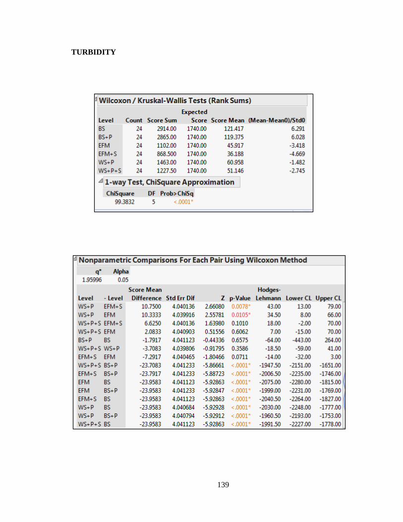
139

TURBIDITY

140

MTSS

141

D.2.TEST PERIOD II RESULTS

RUNOFF VOLUME

142

TURBIDITY

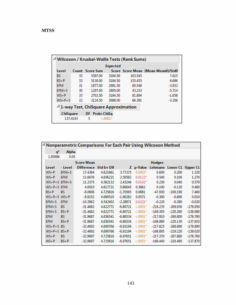
143

MTSS

144

D.3. COMPARISON OF SEEDED VS. NON-SEEDED TREATMENTS

RUNOFF VOLUME

Source Sum of Squares Df Mean Square F-Ratio P-Value

DAS 4.91984E6 1 4.91984E6 1.63 0.2055

Intercepts 4.09822E7 1 4.09822E7 13.60 0.0004

Slopes 1.57479E7 1 1.57479E7 5.22 0.0252

Model 6.16499E7 3

145

TURBIDITY


DAS 22277.1 1 22277.1 3.39 0.0696

Intercepts 11785.3 1 11785.3 1.80 0.1845

Slopes 40160.2 1 40160.2 6.12 0.0158

Model 74222.6 3

146

MTSS


DAS 4.59036 1 4.59036 9.71 0.0027

Intercepts 1.49443 1 1.49443 3.16 0.0799

Slopes 5.13707 1 5.13707 10.86 0.0016

Model 11.2219 3

Effectiveness of selected erosion control covers during ...

Documents

Transcript of Effectiveness of selected erosion control covers during ...