Publications (YM) Yucca Mountain

2008

Final report: Phase stability and segregation in Alloy 22 base Final report: Phase stability and segregation in Alloy 22 base

metal and weldments metal and weldments

Jeffrey LaCombe University of Nevada, Reno, lacomj@unr.edu

Follow this and additional works at: https://digitalscholarship.unlv.edu/yucca_mtn_pubs

Part of the Metallurgy Commons

Repository Citation Repository Citation LaCombe, J. (2008). Final report: Phase stability and segregation in Alloy 22 base metal and weldments. Available at:Available at: https://digitalscholarship.unlv.edu/yucca_mtn_pubs/19

This Technical Report is protected by copyright and/or related rights. It has been brought to you by Digital Scholarship@UNLV with permission from the rights-holder(s). You are free to use this Technical Report in any way that is permitted by the copyright and related rights legislation that applies to your use. For other uses you need to obtain permission from the rights-holder(s) directly, unless additional rights are indicated by a Creative Commons license in the record and/or on the work itself. This Technical Report has been accepted for inclusion in Publications (YM) by an authorized administrator of Digital Scholarship@UNLV. For more information, please contact digitalscholarship@unlv.edu.

Final Report:Task: ORD-FY04-015

Phase Stability and Segregation in Alloy 22Base Metal and Weldments

J.C. LaCombe1

Chemical and Metallurgical EngineeringUniversity of Nevada, Reno,

Reno, NV 89557 USA

abstract abstract abstract abstract abstract abstract abstract abstract abstract abstractabstract abstract abstract abstract abstract abstract abstract abstract abstract abstractabstract abstract abstract abstract.

Project Background

At the outset of this project, the design of the waste disposal containers relied heavily onencasement in a multi-layered container, featuring a corrosion barrier of Alloy 22, a Ni-Cr-Mo-W based alloy with excellent corrosion resistance over a wide range of conditions. Thefundamental concern from the perspective of the Yucca Mountain Project, however, was theinherent uncertainty in the (very) long-term stability of the base metal and welds. Shouldthe properties of the selected materials change over the long service life of the waste packages,it was conceivable that the desired performance characteristics (such as corrosion resistance)would become compromised, leading to premature failure of the system. To address this,we studied aspects of the phase stability and solute segregation characteristics of Alloy 22base metal, and the manner in which these affected corrosion resistance. This work wasconducted as an independent validation, to add to confidence in the extrapolated behaviorof the container materials over time periods that are not feasibly tested in a laboratory.

Ni base alloys with 16-22% chromium and 9-16% molybdenum are commonly used forhigher corrosion resistance applications. Alloy-22 (UNS N06022), a Ni-Cr-Mo-W alloy, isthe current reference material for construction of the outer wall of nuclear waste containers[1, 2, 3, 4] to be used by the Yucca Mountain Project. The nominal composition of Alloy-22and the compositions of some of the reported phases seen in this alloy system are listed inTable .

Even though Alloy-22 in wrought form is considered to have good phase stability at theoperating temperatures < 200 ◦C of the repository, exposure to elevated temperatures duringthe fabrication processes (such as welding and stress relieving) could cause alteration ofmicrostructure and associated deterioration of mechanical and corrosion properties. Weldingcauses microstructural changes in Alloy-22, such as formation of dendrites in the weld metal,segregation of Mo and W in the interdendritic regions, formation of topologically close packedphases both in the weld metal and the heat affected zone (HAZ), and possibly precipitation

1To whom correspondence should be addressed: e-mail lacomj@unr.edu.

1

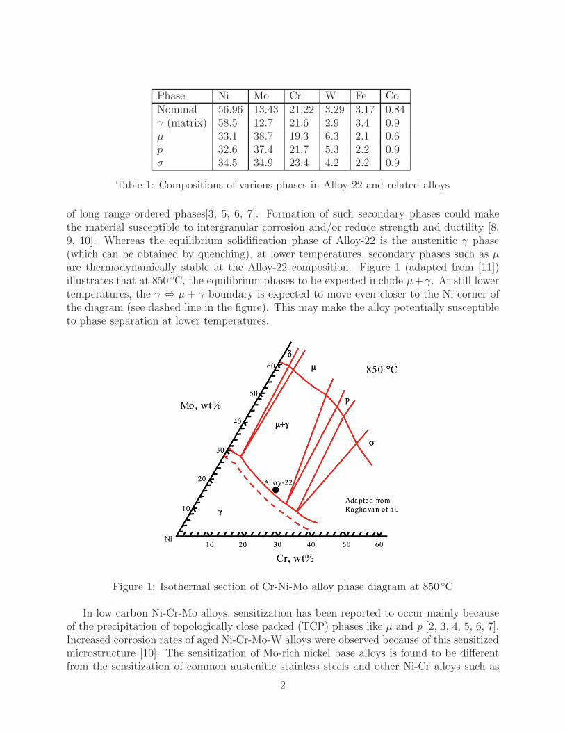
Phase Ni Mo Cr W Fe CoNominal 56.96 13.43 21.22 3.29 3.17 0.84γ (matrix) 58.5 12.7 21.6 2.9 3.4 0.9μ 33.1 38.7 19.3 6.3 2.1 0.6p 32.6 37.4 21.7 5.3 2.2 0.9σ 34.5 34.9 23.4 4.2 2.2 0.9

Table 1: Compositions of various phases in Alloy-22 and related alloys

of long range ordered phases[3, 5, 6, 7]. Formation of such secondary phases could makethe material susceptible to intergranular corrosion and/or reduce strength and ductility [8,9, 10]. Whereas the equilibrium solidification phase of Alloy-22 is the austenitic γ phase(which can be obtained by quenching), at lower temperatures, secondary phases such as μare thermodynamically stable at the Alloy-22 composition. Figure 1 (adapted from [11])illustrates that at 850 ◦C, the equilibrium phases to be expected include μ+γ. At still lowertemperatures, the γ ⇔ μ + γ boundary is expected to move even closer to the Ni corner ofthe diagram (see dashed line in the figure). This may make the alloy potentially susceptibleto phase separation at lower temperatures.

Figure 1: Isothermal section of Cr-Ni-Mo alloy phase diagram at 850 ◦C

In low carbon Ni-Cr-Mo alloys, sensitization has been reported to occur mainly becauseof the precipitation of topologically close packed (TCP) phases like μ and p [2, 3, 4, 5, 6, 7].Increased corrosion rates of aged Ni-Cr-Mo-W alloys were observed because of this sensitizedmicrostructure [10]. The sensitization of Mo-rich nickel base alloys is found to be differentfrom the sensitization of common austenitic stainless steels and other Ni-Cr alloys such as

2

Inconel 600. Sensitization of austenitic stainless steel resulted in depletion of chromiumadjacent to the chromium rich M23C6 carbides [12, 13]. In the Ni-Cr-Mo alloys, sensitizationresulted in depletion of molybdenum near the TCP or M6C precipitates [10, 14]. When thesensitized Ni-Cr-Mo alloys were exposed to a reductive environment the Mo depleted regionswere preferentially attacked and in an oxidizing environment the TCP phases themselveswere dissolved, giving rise to the corrosion rate [14]. Raghavan et al. [11] and Cieslaket al. [5, 6, 7] observed the TCP phases containing only the nominal chromium as thatof the bulk chemistry. Whereas, Hodge [14, 15] reported that the μ phase was enrichedwith Cr and the suggested phase was (Ni, Fe, Co)3(W, MO, Cr)2. This issue is not fullyresolved as of yet. There are no reports available on the depletion profiles of aged Alloy-22.Depletion of alloying elements in the vicinity of secondary phase precipitates will impair thecorrosion resistance of the alloy. Therefore, it is imperative to develop an understanding ofhow the microstructure changes during fabrication or exposure to service conditions so thatthe integrity of the waste package container can be ensured.

The three principal efforts of this project were:

Subtask 1: Microstructural Characterization of Phase Stability and Vari-ability in Alloy 22 Develop an improved understanding of Alloy 22 and the extent towhich compositional and microstructural variations are present in otherwise nominalas-procured material.

Subtask 2: Electrochemical Methods to Detect Susceptibility of Alloy 22to Localized Corrosion Study the influence that compositional and microstructuralvariations have on the corrosion performance of Alloy 22.

Subtask 3: Multicomponent Diffusivity of Alloy 22 Preliminary investigationof the role of diffusion in Alloy-22 at repository temperatures (scoping study).

Subtask 1: Microstructure

The principal goal of Subtask 1 was to develop an improved understanding of Alloy 22 andthe extent to which compositional and microstructural variations are present in otherwisenominal as-procured material. This involved the following questions

1. Characterize the as-fabricated Alloy-22 base metal.

2. Characterize Alloy-22 welds (goal eliminated mid-project)

3. Long-term metallurgical stability: Cr-Mo depletion and Long Range Ordering

4. Segregation of sulfur and phosphorous.

This research has studied the microstructural variabilities in Alloy 22 using various char-acterization techniques. Light optical, scanning electron, and transmission electron mi-croscopy techniques were used to metallurgically examine the characteristics of secondaryphases. The conclusions are summarized, as follows:

3

1. Light optical microscope micrographs exhibited expected precipitate formation at sen-sitizing conditions and dissolution at solutionizing conditions, as predicted by theequivalent element ternary Ni-Cr-Mo phase diagram and observations from other re-searchers. Increases of precipitation with temperature were not intensely observed.

2. Scanning electron microscopy with energy-dispersive X-ray spectroscopy confirmed thedepletion of nickel, chromium, and tungsten along with segregation of molybdenum,within a grain boundary, but not accurate enough to differentiate the type of phase.These material compositional variations give some confidence on the presence of pre-cipitates but limited since using etched specimens.

3. Transmission electron microscopy with energy-dispersive X-ray spectroscopy resultsdid not match previous works exactly, complexity of Alloy 22 element composition isspeculated to be at fault, but did closely follow the characteristics of the ? phase. Thisresult was expected from the ternary phase diagrams for Ni-Cr-Mo and from otherresearchers.

4. Microhardness measurements indicated no significant changes with increasing sensitiz-ing durations, only a 10% hardness increase was observed with increasing sensitizingtemperatures. Macrohardness measurements displayed less variability, compared tomicrohardness, and did increase with higher temperatures and sensitizing durations.Since the sensitizing temperatures were not in range of long-range ordering formations,the only contributing factors to hardness increase are with carbides and secondaryphases. The hardness values agree with previous works. Large deviations from themicrohardness testing are due to the grain-to-grain variability and are not sufficient tomeasure precipitate formation as functions of time and temperature.

5. Grain size measurements were conducted for Alloy 22 specimens in the as-received,sensitized, and solutionized conditions. Comparisons for each category showed trendswith unpredictable behaviors caused by either the ambiguous duplex microstructureof the alloy, or the large confidence intervals of the data sets. Grain growth kineticscould not be adequately confirmed.

6. Phase fraction analysis proved to be successful using backscattered SEM micrographsand Scentis software, despite only using one specimen. Resulting data is not sufficientfor precipitate growth and dissolution conclusions.

7. All measurements included moderately high standard deviations due to the influence ofdata outliers, which is expected in small data sets. Results have shown that an increasein data points can lead to more statistically significant results. Specific measurementtechniques have been developed in this research and are expected to continue withlager data sets in future works.

8. The long-term metallurgical stability of Alloy 22 is dependent on the dissolution ofsecondary phases, since the increase of temperature and time during sensitizing heattreatments has been shown to influence precipitation and accumulate in the grain

4

boundaries leading to saturation in the bulk material. Limitations must be consideredfor the control of energies introduced into the material during production or fabrication.

Subtask 2: Corrosion

Goals

The main mode of corrosion that may occur at the repository site was examined here. Alloy-22 (C-22) is a versatile nickel-chromium-molybdenum-tungsten alloy with good overall cor-rosion resistance. It is claimed that C-22 alloy has outstanding resistance to pitting, crevicecorrosion, and stress corrosion cracking. Intergranular corrosion and exposure of Alloy-22 tomoderately elevated temperatures may potentially lead to diminished corrosion resistance anissue that we examine here. The intergranular corrosion resistance of Alloy-22 after variousheat treatments on both mill annealed and welded samples was studied using ASTM G28tests. We attempted to corroborate these results using suitable methods such as double-loopelectrochemical potentiokinetic reactivation (EPR) tests, as well as material characterizationtechniques including optical microscopy, scanning electron microscopy (SEM), and energydispersive spectrometry (EDS). The samples were tested using electrochemical potentioki-netic reactivation (EPR) tests in solutions that were developed specifically so as to check forchromium and molybdenum depletion.

Alloy 22 is considered to be less susceptible to Localized corrosion (LC), due to theadditions of Mo and W, both of which are believed to stabilize the passive film at verylow pH. The oxides of these elements are believed to be very insoluble at low pH, as aresult of which Alloy 22 is believed to exhibit relatively high thresholds for localized attack[18]. Alloy-22 (UNS N06022) is said to rely on the stability of a thin chromium oxide filmfor protection against corrosion [19]. Alloy 22 was supposedly designed to resist the mostaggressive industrial applications, offering a low general corrosion rate under both oxidizingand reducing conditions [20]. It is believed that Chromium exerts its beneficial effect in thealloy under oxidizing and acidic conditions, under reducing conditions the most beneficialalloying elements are molybdenum and tungsten which offer a low exchange current densityfor hydrogen discharge. Alloy 22 is believed to be an excellent alternative to austeniticstainless steels that may fail by pitting corrosion or stress corrosion cracking (SCC) in hotchloride containing solutions due to its balanced content in chromium, molybdenum andtungsten [21, 22].

The principal goal of Subtask 2 was to study the influence that compositional and mi-crostructural variations have on the localized corrosion performance of Alloy 22. This wasdivided into smaller goals.

1. Develop an EPR test solution and Cr depletion test procedure

2. Develop an electrochemical test solution and Mo segregation test procedure

3. Study the effect of precipitation of secondary phases on the corrosion resistance ofAlloy-22

5

Results: Chemical Weight Loss Tests

ASTM G 28 Chemical Weight Loss Test Results Discussion

The test results were consistent with the results that were reported by Gorhe et.al [23]. Thesample that was sensitized at 650 ◦C for 60 minutes showed a corrosion rate of 22.83 mpyafter the ASTM-G-28-A test. Gorhe et.al [23] reported a corrosion rate of 21.98 mpy for anAlloy 22 sample that was given a similar heat treatment after a similar test. Another samplethat was sensitized at 750 ◦C for 60 minutes showed a corrosion rate of 27.29 mpy after theASTM-G-28-A test close to the corrosion rate of 30.57 mpy obtained by Gorhe et.al [23].Alloy 22 samples that were sensitized at 700 ◦C for about 6000 minutes showed a corrosionrate of 151.98 mpy after the ASTM-G-28-A test as reported by Gorhe et.al [23]. Whileour tests on a sample given the similar heat treatment for the same time showed a lessercorrosion rate of 46.56 mpy. In the ASTM-G-28-B tests that were done on Alloy 22 samplessensitized at 650 ◦C, 70 ◦C for 60 minutes showed corrosion rates of 40.51mpy, 2070.59 mpyafter the ASTM-G-28-B tests respectively. Gorhe et.al [23] reported lower corrosion ratesof 5.2 mpy, 47.64 mpy after the ASTM-G-28-B tests for similar samples respectively. Thesamples that were sensitized at 650 ◦C and 750 ◦C for about 6000 minutes showed corrosionrates of 3179.58 mpy, 3504.72 mpy after the ASTM-G-28-B tests in our work which weresimilar to the results obtained by Gorhe et.al [23] which are 3398.82 mpy, 4002.76 mpyrespectively on samples given the similar heat treatments after the similar test.

Mill Annealed Condition

The samples in the mill-annealed condition showed corrosion rates ranging from 5.11 mpyto 29.52 mpy for different samples after the ASTM-G-28-A test. The ASTM-G-28-B testresults showed corrosion rates ranging from 3.96 mpy to 26.55 mpy for various mill-annealedAlloy-22 samples.

Sensitized Condition

The ASTM-G-28-A test results for the Alloy 22 samples after being sensitized at varioustemperatures for 60 minutes showed a clear trend of increase in the corrosion rate withincrease in the temperature of sensitization from 650 ◦C all the way to 750 ◦C. The corrosionrate values after the ASTM-G-28-A test for the samples sensitized for 60 minutes increasedfrom 18.4 mpy from an Alloy 22 sample sensitized at 650 ◦C to 27.29 mpy for an Alloy 22sample sensitized at 750 ◦C. Although ASTM-G-28-A test results for samples sensitized for600 minutes showed corrosion rates of 26.26 mpy at a sensitization temperature of 650 ◦C anda corrosion rate of 23.96 mpy at a sensitization temperature of 750 ◦C. The corrosion ratevalues after the ASTM-G-28-A test for the samples sensitized for 60 minutes increased from18.4 mpy from an Alloy 22 sample sensitized at 650 ◦C to 27.29 mpy for an Alloy 22 samplesensitized at 750 ◦C. The corrosion rate values after the ASTM-G-28-A test for the samplessensitized for 6000 minutes increased from 46.56 mpy from an Alloy 22 sample sensitizedat 700 ◦C to 91.58 mpy for an Alloy 22 sample sensitized at 850 ◦C which again shoed therelevance of increase in the temperature of sensitization on the corrosion rates. There wasnt

6

0

10

20

30

40

50

60

70

80

90

100

15 60 600

Corr

osi

on R

ate

(mpy)

Alloy 22ASTM G-28-A Test Results650, 700, 750, 850, 1125,1150, 1175- Temperatures of Heat Treatment in °C.

1150°C

1175°C1125°

C

650°C 650°C

750°C

750°C

1150°C

1175°C

650°C750°C

700°C

800°C

Figure 2: ASTM-G28A Chemical Weight Loss Test Results

such a clear effect of the time of sensitization on the corrosion rate though the averagecorrosion rate of the various samples done for every segment of the time of sensitizationclearly increased in the direction of the larger times of sensitization. The ASTM-G-28-Atest results for the various sensitized samples/batches obtained from different manufacturersshowed almost similar results. For example the ASTM-G-28-A test results for two differentAlloy 22 samples, both sensitized at 750 ◦C for 60 minutes showed corrosion rates of 18.4,21.84 mpy respectively. The ASTM-G-28-B test results for the Alloy 22 samples after beingsensitized at various temperatures for 60 minutes showed a clear trend of increase in thecorrosion rate with increase in the temperature of sensitization from 650 ◦C all the way to750 ◦C. The corrosion rate values after the ASTM-G-28-A test for the samples sensitized for60 minutes increased from 40.51 mpy from an Alloy 22 sample sensitized at 650 ◦C to 3504.72mpy for an Alloy 22 sample sensitized at 750 ◦C. The corrosion rate value after the ASTM-G-28-B test for the samples sensitized for 60000 minutes showed a corrosion rate of 3023.71mpy for an Alloy 22 sample sensitized at 850 ◦C which again showed the relevance of increasein the temperature of sensitization on the corrosion rates. There was also a clear effect ofthe time of sensitization on the corrosion rate with the average corrosion rate of the varioussamples done for every segment of the time of sensitization clearly increasing in the directionof the larger times of sensitization. The ASTM-G-28-B test results for the various sensitizedsamples/batches obtained from different manufacturers showed almost similar results. Forexample the ASTM-G-28-B test results for three different Alloy 22 samples, all sensitized at750 ◦C for 6000 minutes showed corrosion rates of 2978.73, 2774.09, 3504.72 mpy respectively.In general the average corrosion rates of sensitized samples of Alloy 22 were about 100 timeshigher for the ASTM-G-28-B test compared to the ASTM-G-28-A tests.

The results of the ASTM-G28A tests of sensitized samples are summarized in Figure 2.Similarly, the results of the ASTM-G28B sensitized tests are summarized in Figure 3.

7

1

10

100

1000

15 60 6000 60000

Co

rro

sio

n R

ate

(In m

py)

Heat Treatment Time (In Min)

1125°C

650°C

750°C

1175°C 650°

C650°C

750°C

750°C650°

C

750°C

850°C

Figure 3: ASTM-G28B Chemical Weight Loss Test Results

Solutionized Condition

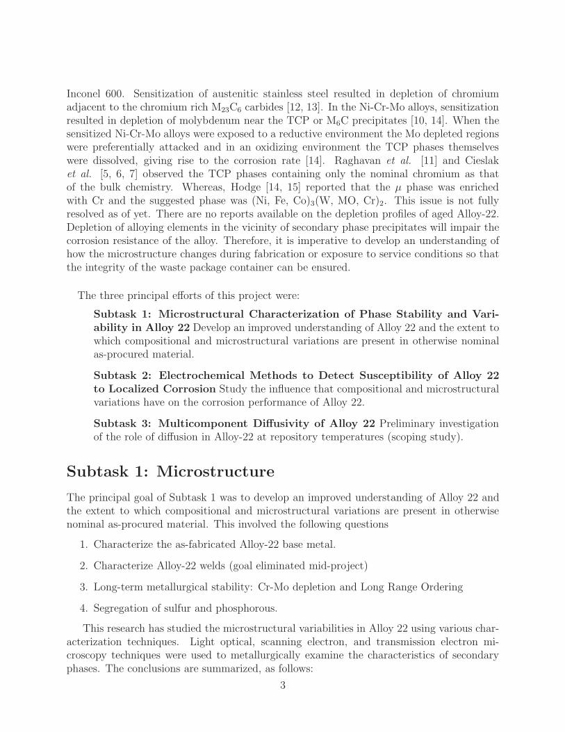
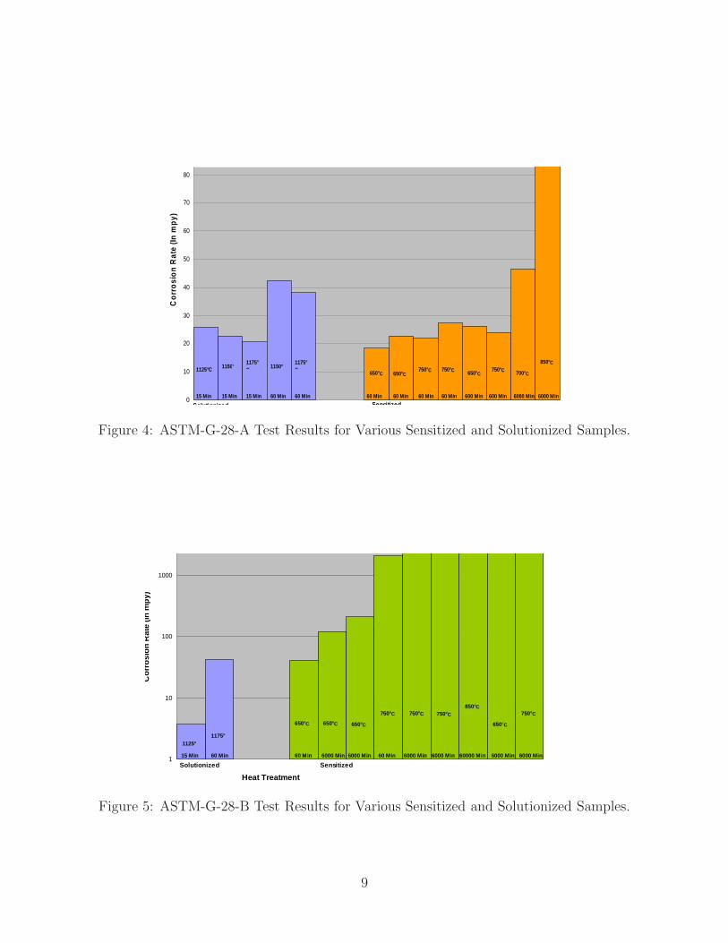
The ASTM-G-28-A test results for the various Alloy 22 samples that were given solution heattreatment showed a clear trend of decreasing corrosion rates with increase in temperature.The corrosion rates for three different Alloy 22 samples that were solutionized for 15 minutesat temperatures of 1125 ◦C, 1150 ◦C, 1175 ◦C showed corrosion rates of 25.93, 22.76, 20.64mpy respectively. The average corrosion rate though definitely increased with increase inthe time of solution treatment in minutes. Again at 60 minutes of solution treatment Alloy22 showed higher corrosion rate for solution treatment at 1150 ◦C compared to the solutiontreatment at 1175 ◦C. The solution heat treatment showed corrosion rates that peakedat lower temperatures for higher times of heat treatment compared to the sensitizationtreatment that showed corrosion rates which peaked at both higher temperatures and timesof sensitizations. The maximum corrosion rates though were the highest in sensitized samplesand the average corrosion rate was also higher in sensitized samples. The ASTM-G-28-Btest results for the various Alloy 22 samples that were given solution heat treatment showeda higher corrosion rate for a sample with increase in the time of solution treatment as well asthe temperature. The solution heat treatment showed corrosion rates that peaked at highertemperatures for higher times of heat treatment just like the sensitization treatment thatshowed corrosion rates which peaked at both higher temperatures and times of sensitizations.The maximum corrosion rates though were the highest in sensitized samples and the averagecorrosion rate was also higher in sensitized samples for the ASTM-G-28-B tests.

A comparison of sensitized and solutionized ASTM-G28A test results is shown in Figure5, and for ASTM-G28B in Figure ??. Figures 6 (ASTM-G28A) and 7(ASTM-G28B) showvariations in chemical weight loss for several manufacturers.

8

0

10

20

30

40

50

60

70

80C

orr

osi

on

Rat

e (In

mp

y)

Solutionized Sensitized

1125°C 1150°1175°C

1150°1175°C

650°C 650°C750°C 750°C 650°C

750°C 700°C

850°C

15 Min 15 Min 15 Min 60 Min 60 Min 60 Min 60 Min 60 Min 60 Min 600 Min 600 Min 6000 Min 6000 Min

Figure 4: ASTM-G-28-A Test Results for Various Sensitized and Solutionized Samples.

1

10

100

1000

Heat Treatment

Co

rro

sio

n R

ate

(In m

py)

Solutionized Sensitized

1125°1175°

650°C 650°C 650°C

750°C 750°C 750°C850°C

650°C

750°C

15 Min 60 Min 60 Min 6000 Min 6000 Min 60 Min 6000 Min 6000 Min 60000 Min 6000 Min 6000 Min

Figure 5: ASTM-G-28-B Test Results for Various Sensitized and Solutionized Samples.

9

0

10

20

30

40

50

60

70

80

Co

rro

sio

n R

ate

(In

mp

y)

Batch-1 Batch-2 Batch-3

750°C

600 Min

650°C 600 Min

700°C

6000 Min 6000 Min

850°C

650°C60 Min 60 Min

750°C650°C

60 Min 60 Min

750°C

Figure 6: ASTM-G-28-A Test Results for Sensitized Samples from Various Batches obtainedfrom Various Manufacturers.

1

10

100

1000

Batches of Alloy-22 from Different Manufacturers

Co

rro

sio

n R

ate

(In

mp

y)

Batch-1 Batch-2 Batch-3

650°C

60 Min 60 Min

750°C 750°C

6000 Min 60000 Min

850°C 650°C

6000 Min 6000 Min

650°C 750°C

6000 Min

650°C

6000 Min

750°C

6000 Min

Figure 7: ASTM-G-28-B Test Results for Sensitized Samples from Various Batches obtainedfrom Various Manufacturers.

10

Results: EPR Tests

Double-Loop EPR Tests in 5 Wt% NaCl Solution (pH-7) at a Temperature of30 ◦C.

Two of the mill-annealed samples showed that the risk of localized corrosion is extremelylow. Even the general corrosion is not predicted, the general corrosion rate may be at most acontamination rate. One mill-annealed sample showed suspected risk of localized corrosionin the form of crevice corrosion which might be present in areas such as close proximity ofsurfaces, areas under deposits, and metal- silicone O-ring interfaces may be prone to suchattack. But such assumptions can only be conformed using longer term immersion testswith, for example, artificial crevice formers which are implied to confirm crevice corrosionprediction.

In the sensitized samples the samples that was sensitized at 650 C for 60 minutes, sensi-tized at 700C for 600 minutes, sensitized at 700 C for 6000 minutes, 750C for 6000 minutes,700C for 6000 minutes (batch-2) showed that no attack is being predicted. The risk of lo-calized corrosion was extremely low so as to call it negligible. Even general corrosion wasnot predicted at all in these samples. The samples that were sensitized at 650C for 600 min-utes, 750C for 60 minutes showed that the risk of localized corrosion in the form of crevicecorrosion in close proximity of surfaces such as metal-O-ring interfaces etc. might be there.Though longer term immersion tests with, for example, artificial crevice formers are impliedto confirm crevice corrosion prediction.

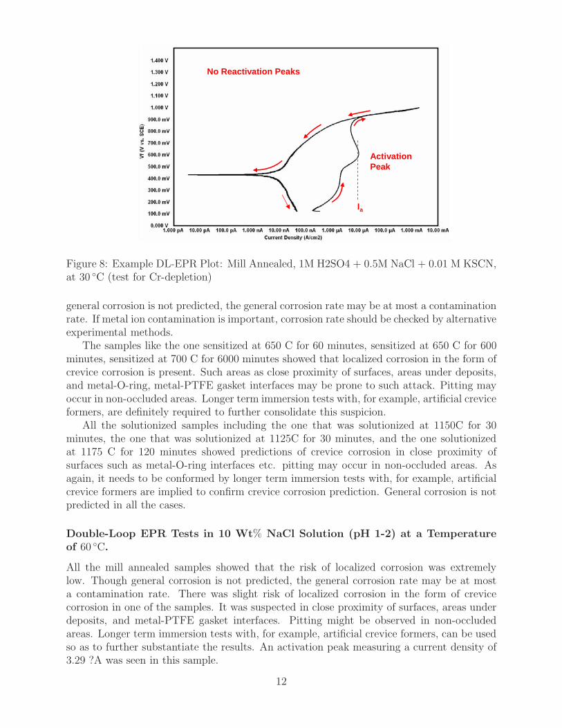
In the solutionized samples the one that was solutionized at 1150C for 30 minutes, andthe one that was solutionized at 1125C for 30 minutes showed predictions of crevice corrosionin close proximity of surfaces such as metal-O-ring interfaces etc. Pitting may occur in non-occluded areas. As again, it needs to be conformed by longer term immersion tests with, forexample, artificial crevice formers are implied to confirm crevice corrosion prediction. Thesample that was solutionized at 1125C for 30 minutes showed a slight activation peak whichwas seen at a current density of 280.7 μA and a reactivation peak at 163.7 μA. The ratioof Ir to Ia was about 0.6. Sensitization at the grain boundaries to a certain extent is beingsuspected. When the Alloy 22 sample was solutionized at 1175C for 120 minutes tracesof general corrosion was suspected. But this needs to be conformed by coupon immersiontesting, electrochemical impedance spectroscopy, or polarization resistance methods whichare suggested to confirm predictions, since corrosion rates cannot be easily estimated frompolarization scans. An example DL-EPR test is depicted in the plot in Figure 8.

Double-Loop EPR Tests in 10 Wt% NaCl Solution (pH-7) at a Temperature of60 ◦C.

As expected all the mill-annealed samples showed that the risk of localized corrosion isextremely low and no attack was predicted. Even the general corrosion is not predicted, thegeneral corrosion rate may be at most a contamination rate.

The samples that were tested including the ones sensitized at 700 C for 600 minutes,sensitized at 750 C for 60 minutes, sensitized at 750 C for 6000 minutes showed risk oflocalized corrosion is extremely low almost that no attack was being predicted. Though

11

No Reactivation Peaks

Activation Peak

Ia

Figure 8: Example DL-EPR Plot: Mill Annealed, 1M H2SO4 + 0.5M NaCl + 0.01 M KSCN,at 30 ◦C (test for Cr-depletion)

general corrosion is not predicted, the general corrosion rate may be at most a contaminationrate. If metal ion contamination is important, corrosion rate should be checked by alternativeexperimental methods.

The samples like the one sensitized at 650 C for 60 minutes, sensitized at 650 C for 600minutes, sensitized at 700 C for 6000 minutes showed that localized corrosion in the form ofcrevice corrosion is present. Such areas as close proximity of surfaces, areas under deposits,and metal-O-ring, metal-PTFE gasket interfaces may be prone to such attack. Pitting mayoccur in non-occluded areas. Longer term immersion tests with, for example, artificial creviceformers, are definitely required to further consolidate this suspicion.

All the solutionized samples including the one that was solutionized at 1150C for 30minutes, the one that was solutionized at 1125C for 30 minutes, and the one solutionizedat 1175 C for 120 minutes showed predictions of crevice corrosion in close proximity ofsurfaces such as metal-O-ring interfaces etc. pitting may occur in non-occluded areas. Asagain, it needs to be conformed by longer term immersion tests with, for example, artificialcrevice formers are implied to confirm crevice corrosion prediction. General corrosion is notpredicted in all the cases.

Double-Loop EPR Tests in 10 Wt% NaCl Solution (pH 1-2) at a Temperatureof 60 ◦C.

All the mill annealed samples showed that the risk of localized corrosion was extremelylow. Though general corrosion is not predicted, the general corrosion rate may be at mosta contamination rate. There was slight risk of localized corrosion in the form of crevicecorrosion in one of the samples. It was suspected in close proximity of surfaces, areas underdeposits, and metal-PTFE gasket interfaces. Pitting might be observed in non-occludedareas. Longer term immersion tests with, for example, artificial crevice formers, can be usedso as to further substantiate the results. An activation peak measuring a current density of3.29 ?A was seen in this sample.

12

The samples like the one sensitized at 650 C for 600 minutes, sensitized at 750 C for600 minutes, sensitized at 700 C for 6000 minutes, sensitized at 750 C for 600 minutesshowed that localized corrosion in the form of crevice corrosion is present. Such areas asclose proximity of surfaces, areas under deposits, and metal-O-ring, metal-PTFE gasketinterfaces may be prone to such attack. Pitting may occur in non-occluded areas. Longerterm immersion tests with, for example, artificial crevice formers, are definitely required tofurther consolidate this suspicion. No general corrosion was predicted in these samples. Aslight activation peak was seen at a current density of 1.48 μA in the forward direction inthe sample that was sensitized at 700 C for 6000 minutes. The sample sensitized at 700C for 600 minutes showed no risk of localized corrosion at all. The sample sensitized at750 C for 60 minutes showed suspected measurable general corrosion rate. This needs to besubstantiated using alternative measurements of corrosion rate by coupon immersion testing,electrochemical impedance spectroscopy, or polarization resistance methods which are usedto confirm predictions. In the Alloy 22 sample that was sensitized at 750 C for 6000minutesan activation peak at the current density Ia of 20.25 μA was seen. A reactivation peak wasalso seen in the reverse direction at a current density Ir of 3.281 μA. The ratio of Ir to Ia isabout 0.17 indicating sensitization at the grain boundary.

The solutionized samples that was solutionized at 1150C for 30 minutes showed extremelylow risk of localized corrosion and no general corrosion was predicted., the one that wassolutionized at 1125C for 30 minutes although showed borderline crevice corrosion whichmight occur at the metal-O-ring interface, and the one solutionized at 1175 C for 120 minutesshowed predictions of crevice corrosion in close proximity of surfaces such as metal-O-ringinterfaces etc. pitting may occur in non-occluded areas. As again, it needs to be conformedby longer term immersion tests with, for example, artificial crevice formers are implied toconfirm crevice corrosion prediction. General corrosion is not predicted in all the cases. Nogeneral corrosion was predicted even in this case.

Double-Loop EPR Tests in 10 Wt% NaCl Solution (pH 13-14) at a Temperatureof 60 ◦C.

Two of the mill annealed samples showed that the risk of localized corrosion was extremelylow. Though general corrosion is not predicted in one of these samples, there is a suspectedgeneral corrosion rate that may be predicted to be measurable in the other one. Alternativemeasurements of corrosion rate like coupon immersion testing, electrochemical impedancespectroscopy, or polarization resistance methods are suggested to confirm these predictionssince corrosion rates cannot be easily estimated from polarization scans.

A slight activation peak was seen measuring a current density Ia of about 54.97 μA inthis sample. A slight activation peak was seen measuring a current density Ia of about 6.12μA was seen in the other sample. There was borderline risk of localized corrosion in theform of crevice corrosion in the third sample. It was suspected in close proximity of surfaces,areas under deposits, and metal-PTFE gasket interfaces Longer term immersion tests with,for example, artificial crevice formers, can be used so as to further substantiate the results.A fourth sample showed no signs of neither localized corrosion nor general corrosion.

The samples like the one sensitized at 650 C for 60 minutes, sensitized at 650 C for 600

13

minutes, sensitized at 700 C for 600 minutes that the risk of localized corrosion is extremelylow to the extent that it is almost negligible. Though general corrosion is not predicted, thegeneral corrosion rate may be at most a contamination rate. If metal ion contamination isimportant, corrosion rate should be checked by alternative experimental methods.

The sample that was sensitized at 700 C for 600 minutes showed suspicions of generalcorrosion although alternative measurements of corrosion rate by coupon immersion testing,electrochemical impedance spectroscopy, or polarization resistance methods are suggested toconfirm predictions since corrosion rates cannot be easily estimated from polarization scans.Localized corrosion in the form of crevice corrosion or pitting is not suggested. An activationpeak was seen during the forward scan at a current density Ia of 3.17 μA and a reactivationpeak at a current density Ir of 1.04 μA giving a ratio of Ir/Ia of 0.33 showing some suspicionof probable activity at the grain boundaries.

The sample that was sensitized at 750 C for about 6000 minutes predicted that, risk oflocalized corrosion in the form of crevice corrosion is present. Such areas as close proximityof surfaces, areas under deposits, and metal-Silicone-O-ring interfaces may be prone to suchattack. Pitting may be observed in non-occluded areas. Longer term immersion tests with,for example, artificial crevice formers, are implied to confirm prediction. No general corrosionwas predicted in this sample. An activation peak was seen during the forward scan at acurrent density Ia of 6.8 A and a reactivation peak at a current density Ir of 2.8 μA givinga ratio of Ir/Ia of 0.41 showing some suspicion of probable activity at the grain boundaries.

In the solutionized samples, the one that was solutionized at 1150C for 30 minutes showedextremely low risk of localized corrosion and no general corrosion was predicted., the onethat was solutionized at 1125C for 30 minutes also showed extremely low risk of localizedcorrosion and no general corrosion was predicted, and the one solutionized at 1175 C for120 minutes showed predictions of general corrosion, although alternative measurementsof corrosion rate, like coupon immersion testing, electrochemical impedance spectroscopy,or polarization resistance methods are suggested to confirm predictions since corrosion ratescannot be easily estimated from polarization scans. Localized corrosion in the form of crevicecorrosion or pitting is not suggested.

Double-Loop EPR Tests for Cr Depletion

The samples that were tested included a mill-annealed sample, sensitized sample at 750 Cfor 600 minutes, sample sensitized at 750C for 6000 minutes, batch-2 sample sensitized at700C for 6000 minutes, and a sample solutionized at 1175C for 120 minutes. All of themshowed that localized corrosion in the form of crevice corrosion or pitting is not suggestedalthough all of them showed mostly activation peaks in the forward direction. Some amountof general corrosion was suspected but alternative measurements of corrosion rate by couponimmersion testing, electrochemical impedance spectroscopy, or polarization resistance meth-ods are suggested to confirm predictions since corrosion rates cannot be easily estimatedusing polarization scans.

The mill-annealed sample showed an activation peak at a current density of 9.173 μA,sensitized sample at 750 C for 600 minutes showed an activation peak at a current densityof 40.08 μA, sample sensitized at 750C for 6000 minutes showed an activation peak at a

14

current density of 62.12 μA, batch-2 sample sensitized at 700C for 6000 minutes showed anactivation peak at a current density of 13.7 μA, and a sample solutionized at 1175C for 120minutes showed an activation peak at a current density of 181.1 μA.

Double-Loop EPR Tests for Mo Depletion

The samples that were tested included a mill-annealed sample, batch-2 sample sensitizedat 700 ◦C. for 6000 minutes. All of them showed that localized corrosion in the form ofcrevice corrosion or pitting is not suggested although all of them showed mostly activationpeaks in the forward direction suggesting. Some amount of general corrosion was suspectedbut alternative measurements of corrosion rate by coupon immersion testing, electrochem-ical impedance spectroscopy, or polarization resistance methods are suggested to confirmpredictions since corrosion rates cannot be easily estimated using polarization scans.

The mill-annealed sample showed an activation peak at a current density of 18.93 μA.

Conclusions of Subtask 2

The results of the ASTM-G-28 chemical weight loss tests were analyzed and plotted so as toobtain a broader understanding of the various correlations between the parameters like heattreatment times, temperatures and sources of the raw metal obtained in the mill annealedcondition. The samples in the mill-annealed condition showed corrosion rates ranging from5.11 mpy to 29.52 mpy for different samples after the ASTM-G-28-A test. The ASTM-G-28-B test results showed corrosion rates ranging from 3.96 mpy to 26.55 mpy for variousmill-annealed Alloy-22 samples. There was also a clear effect of the time of sensitizationon the corrosion rate with the average corrosion rate of the various samples done for everysegment of the time of sensitization clearly increasing in the direction of the larger times ofsensitization. There was again the relevance of increase in the temperature of sensitizationon the corrosion rates. In general the average corrosion rates of sensitized samples of Alloy 22were about 100 times higher for the ASTM-G-28-B test compared to the ASTM-G-28-A tests.The solution heat treatment showed corrosion rates that peaked at lower temperatures forhigher times of heat treatment compared to the sensitization treatment that showed corrosionrates which peaked at both higher temperatures and times of sensitizations. The maximumcorrosion rates though were the highest in sensitized samples and the average corrosion ratewas also higher in sensitized samples. The tests results indicated that the samples are morevulnerable to higher intergranular corrosion as influenced by variations in the parameters forprocessing. The samples in general exhibited higher corrosion rates in ASTM G-28-B tests.

The double-loop EPR (Electrochemical Potentiokinetic Reactivation) test results showedthat all the mill-annealed samples in the various test conditions showed that the risk oflocalized corrosion is extremely low. Even the general corrosion is not predicted, the generalcorrosion rate may be at most a contamination rate. One mill-annealed sample showed sus-pected risk of localized corrosion in the acidic condition that is a form of crevice corrosionwhich might be present in areas such as close proximity of surfaces, areas under deposits,and metal- silicone O-ring interfaces may be prone to such attack. But such assumptionscan only be conformed using longer term immersion tests with, for example, artificial crevice

15

formers which are implied to confirm crevice corrosion prediction. In the basic conditionthough general corrosion is not predicted, in one of the samples, there is a suspected gen-eral corrosion rate that may be predicted to be measurable. Alternative measurements ofcorrosion rate like coupon immersion testing, electrochemical impedance spectroscopy, orpolarization resistance methods are suggested to confirm these predictions since corrosionrates cannot be easily estimated from polarization scans.

Most of the sensitized samples showed that no attack is being predicted. The risk oflocalized corrosion was extremely low so as to call it negligible. Even general corrosion wasnot predicted at all in these samples. Some sensitized samples which were sensitized forlonger periods and higher temperatures showed that the risk of localized corrosion in theform of crevice corrosion in close proximity of surfaces such as metal-O-ring interfaces etc.might be there. Though longer term immersion tests with, for example, artificial creviceformers are implied to confirm crevice corrosion prediction.

Most of the solutionized samples showed that no attack is being predicted. The risk oflocalized corrosion was extremely low so as to call it negligible. Even general corrosion wasnot predicted at all in these samples. Some solutionized samples that were solutionized forlonger periods and higher temperatures showed that the risk of localized corrosion in theform of crevice corrosion in close proximity of surfaces such as metal-O-ring interfaces etc.might be there. Though longer term immersion tests with, for example, artificial creviceformers are implied to confirm crevice corrosion prediction.

Very few of them showed suspected measurable general corrosion rate. This needs to besubstantiated using alternative measurements of corrosion rate by coupon immersion testing,electrochemical impedance spectroscopy, or polarization resistance methods which are usedto confirm predictions.

All the samples that were tested for Cr- depletion, Mo-Depletion showed that localizedcorrosion in the form of crevice corrosion or pitting is not suggested although all of themshowed mostly activation peaks in the forward direction. Some amount of general corrosionwas suspected but alternative measurements of corrosion rate by coupon immersion testing,electrochemical impedance spectroscopy, or polarization resistance methods are suggestedto confirm predictions since corrosion rates cannot be easily estimated using polarizationscans. The ASTM-G-28 Tests are carried out in highly exaggerated conditions that thematerial may not face in the actual repository condition. Although it did show that therewas effect of the processing parameters on the material in its sustained endurance to facecorrosion at these exaggerated conditions. This can be used as an input to look for theexact behavior of Alloy-22 at the exact repository conditions after going through variousprocesses like welding, brazing etc. The Double-Loop EPR tests showed that the materialwas very resistant to localized corrosion in conditions that contained high amounts of chlorideconditions and even the Chromium and Molybdenum depletion wasnt present in higherquantities that could lead to intense localized corrosion. The sensitization at the grainboundaries was minimal as no prominent activation/reactivation peaks were found in almostall the samples. The very minimal activity that was present at the grain boundaries wasmore in the sample that was sensitized at higher temperatures like 750 C for higher periodslike 6000 minutes in highly acidic and basic chloride solutions. A stray case of sensitizationwas seen in one of the solutionized sample. Although these results need to be substantiated

16

using alternative methods like longer term immersion tests with, for example, artificial creviceformers, coupon immersion testing, electrochemical impedance spectroscopy, or polarizationresistance methods etc at the exact repository conditions.

Subtask 3: Diffusion

Goals

The diffusion studies were conducted as non–QA scoping work to complement the otheractivities. This was not (technically) listed as a subtask in the original SIP (only as scopingwork). The goals of this study were as follows.

1. Measure the diffusivity matrix of the ternary equivalent of Alloy–22 at metallurgicaltemperatures near the solutionizing temperature of the alloy.

2. Develop an understanding of what will be necessary in order to determine the diffusivityof this alloy at repository operating conditions. I.e., examine the feasibility of low–temperature measurements.

3. Develop an understanding of the roles of experimental uncertainties in long–term dif-fusion measurements (i.e., at low temperature).

This study was centered on experimental measurements, but involved a considerableamount of theoretical work in order to properly understand the data and the feasibility offuture low–tempearture studies.

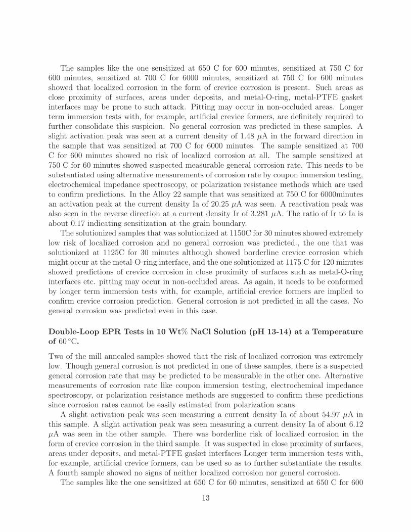
To most efficiently gather and analyze the diffusion couple data, a regression scheme wasdeveloped in–house, which combined both heuristic and nonlinear regression components toprovide a combination of efficient operation with accurate results. This refression schemehas been published in [24]. The scheme is outlined in Figure 9.

Results of Subtask 3

Validation of Regression Methods

The regression method was tested in order to know how well it can reproduce the originaldiffusivity matrix [D]. Validation was done using simulated concentration profiles generatedaccording to expressions from an hypothetical diffusivity matrix.

The element analysis techniques, like EPMA, used here, have an intrinsic uncertaintyleading to errors in the measured value. Therefore, in order to know how the method willbehave considering data scattering, artificial noise was included in the original data in orderto know how the calculated value for [D] varies when compared with the original. The endcompositions for the simulated diffusion couples are presented in Table 2.The different casesevaluated are described below. All cases were simulated for “t = 200h”. The results for thecalculated diffusivity matrix and the square root diffusivity matrix are presented in Tables 3and 4 respectively. Table 5 shows the results for the eigenvalues of the diffusivity matrix and

17

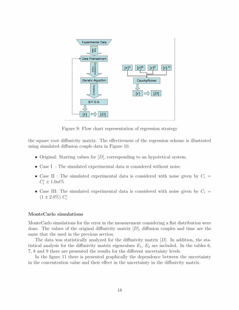
Figure 9: Flow chart representation of regression strategy

the square root diffusivity matrix. The effectiveness of the regression scheme is illustratedusing simulated diffusion couple data in Figure 10.

• Original: Starting values for [D], corresponding to an hypotetical system.

• Case I : The simulated experimental data is considered without noise.

• Case II : The simulated experimental data is considered with noise given by Ci =Cc

i ± 1.0at%

• Case III: The simulated experimental data is considered with noise given by Ci =(1 ± 2.0%) Cc

i

MonteCarlo simulations

MonteCarlo simulations for the error in the measurement considering a flat distribution weredone. The values of the original diffusivity matrix [D], diffusion couples and time are thesame that the used in the previous section.

The data was statistically analyzed for the diffusivity matrix [D]. In addition, the sta-tistical analysis for the diffusivity matrix eigenvalues E1, E2 are included. In the tables 6,7, 8 and 9 there are presented the results for the different uncertainty levels.

In the figure 11 there is presented graphically the dependence between the uncertaintyin the concentration value and their effect in the uncertainty in the diffusivity matrix.

18

Table 2: End compositions for simulated experimental data, in %at

Couple # 1 Couple # 2C−

i C+i C−

i C+i

Element 1 30 55 25 20Element 2 45 25 30 40Element 3 25 20 45 40

Table 3: Diffusivity Matrix: Original and Calculated Data. All the values are in 10−11[cm2/s

][D] Original Case I Case II CaseIII

D11 12.1 12.1 14.8 12.6D12 5.16 5.14 7.82 5.76D21 1.74 1.74 -2.15 0.244D22 6.25 6.25 2.21 4.74

Table 4: Square Root Diffusivity Matrix: Original and Calculated Data. All the values are in10−6

[cm2/s

][r] Original Case I Case II CaseIII

r11 10.9 10.9 12.4 11.2r12 2.75 2.76 4.44 3.19r21 .934 0.933 -1.22 0.135r22 7.74 7.74 5.25 6.85

Table 5: Eigenvalues for the diffusivity matrix and the square root diffusivity matrix. The diffu-sivity matrix eigenvalues Ei are in

[cm2/s

], the square root matrix eigenvalues ei are in

[cm/s1/2

]

Original Case II CaseIII

E1/10−11 13.4 13.3 12.8E2/10−11 4.99 3.73 4.57

Original Case II CaseIII

e1/10−6 11.6 11.5 11.3e2/10−6 7.06 6.11 6.77

Table 6: Statistical results for uncertainty analysis for η = 0.1%. All values are in(10−11

[cm2/s

])η = 0.1%

D11 D12 D21 D22 E1 E2

Mean 12.1 5.13 1.74 6.25 13.4 5.00Median 12.1 5.13 1.75 6.26 13.4 5.00Standard Deviation .0849 .0938 .0663 .0728 .0893 .0260Coefficient of Variation .00700 .0183 .0381 .0117 .00668 .00520

19

Figure 10: Concentration profiles for simulated diffusion couples, for a simulation time of 200hours. Dots correspond to simulated data, and the continuous lines correspond to calculated data.a)Diffusion Couple #1, Case I; b) Diffusion Couple #2, Case I; c) Diffusion Couple #1, Case II; d)Diffusion Couple #2, Case II; e) Diffusion Couple #1, Case III; f) Diffusion Couple #2, Case III.

Table 7: Statistical results for uncertainty analysis for η = 0.2%. All values are in(10−11

[cm2/s

])η = 0.2%

D11 D12 D21 D22 E1 E2

Mean 12.1 5.15 1.73 6.24 13.4 4.99Median 12.1 5.16 1.73 6.24 13.4 5.00Standard Deviation .154 .169 .121 .131 .158 .0463Coefficient of Variation .0127 .0329 .0697 .0210 .0118 .00928

20

Table 8: Statistical results for uncertainty analysis for η = 0.5%. All values are in(10−11

[cm2/s

])η = 0.5%

D11 D12 D21 D22 E1 E2

Mean 12.1 5.12 1.73 6.24 13.4 5.00Median 12.1 5.10 1.76 6.27 13.3 5.01Standard Deviation .438 .489 .341 .372 .466 .131Coefficient of Variation .0361 .0954 .197 .0597 .0348 .0262

Table 9: Statistical results for uncertainty analysis for η = 1.0%. All values are in(10−11

[cm2/s

])η = 1.0%

D11 D12 D21 D22 E1 E2

Mean 12.0 4.96 1.71 6.23 13.2 5.01Median 12.0 4.99 1.71 6.23 13.3 5.01Standard Deviation 1.02 1.13 .649 .713 1.13 .280Coefficient of Variation .0853 .228 .379 .115 .0858 .0559

0 0.1 0.2 0.3 0.4 0.5 0.6 0.7 0.8 0.9 10

0.2

0.4

0.6

0.8

1

η

Stan

dar

Dev

iati

onσ

D11

D12

D21

D22

Figure 11: Standard deviation for the diffusivity matrix at different levels of uncertainty in theconcentration

21

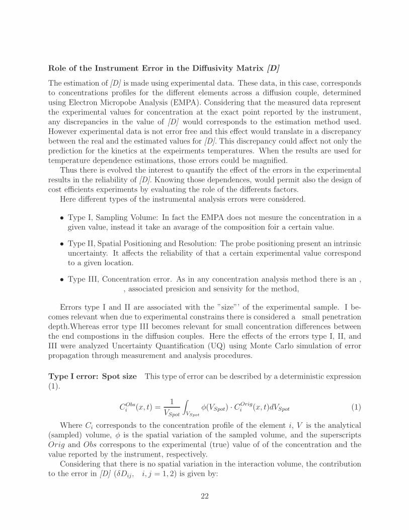
Role of the Instrument Error in the Diffusivity Matrix [D]

The estimation of [D] is made using experimental data. These data, in this case, correspondsto concentrations profiles for the different elements across a diffusion couple, determinedusing Electron Micropobe Analysis (EMPA). Considering that the measured data representthe experimental values for concentration at the exact point reported by the instrument,any discrepancies in the value of [D] would corresponds to the estimation method used.However experimental data is not error free and this effect would translate in a discrepancybetween the real and the estimated values for [D]. This discrepancy could affect not only theprediction for the kinetics at the expeirments temperatures. When the results are used fortemperature dependence estimations, those errors could be magnified.

Thus there is evolved the interest to quantify the effect of the errors in the experimentalresults in the reliability of [D]. Knowing those dependences, would permit also the design ofcost efficients experiments by evaluating the role of the differents factors.

Here different types of the instrumental analysis errors were considered.

• Type I, Sampling Volume: In fact the EMPA does not mesure the concentration in agiven value, instead it take an avarage of the composition foir a certain value.

• Type II, Spatial Positioning and Resolution: The probe positioning present an intrinsicuncertainty. It affects the reliability of that a certain experimental value correspondto a given location.

• Type III, Concentration error. As in any concentration analysis method there is an ,sometimes know, associated presicion and sensivity for the method,

Errors type I and II are associated with the ”size”’ of the experimental sample. I be-comes relevant when due to experimental constrains there is considered an small penetrationdepth.Whereas error type III becomes relevant for small concentration differences betweenthe end compostions in the diffusion couples. Here the effects of the errors type I, II, andIII were analyzed Uncertainty Quantification (UQ) using Monte Carlo simulation of errorpropagation through measurement and analysis procedures.

Type I error: Spot size This type of error can be described by a deterministic expression(1).

CObsi (x, t) =

1

VSpot

∫VSpot

φ(VSpot) · COrigi (x, t)dVSpot (1)

Where Ci corresponds to the concentration profile of the element i, V is the analytical(sampled) volume, φ is the spatial variation of the sampled volume, and the superscriptsOrig and Obs correspons to the experimental (true) value of of the concentration and thevalue reported by the instrument, respectively.

Considering that there is no spatial variation in the interaction volume, the contributionto the error in [D] (δDij, i, j = 1, 2) is given by:

22

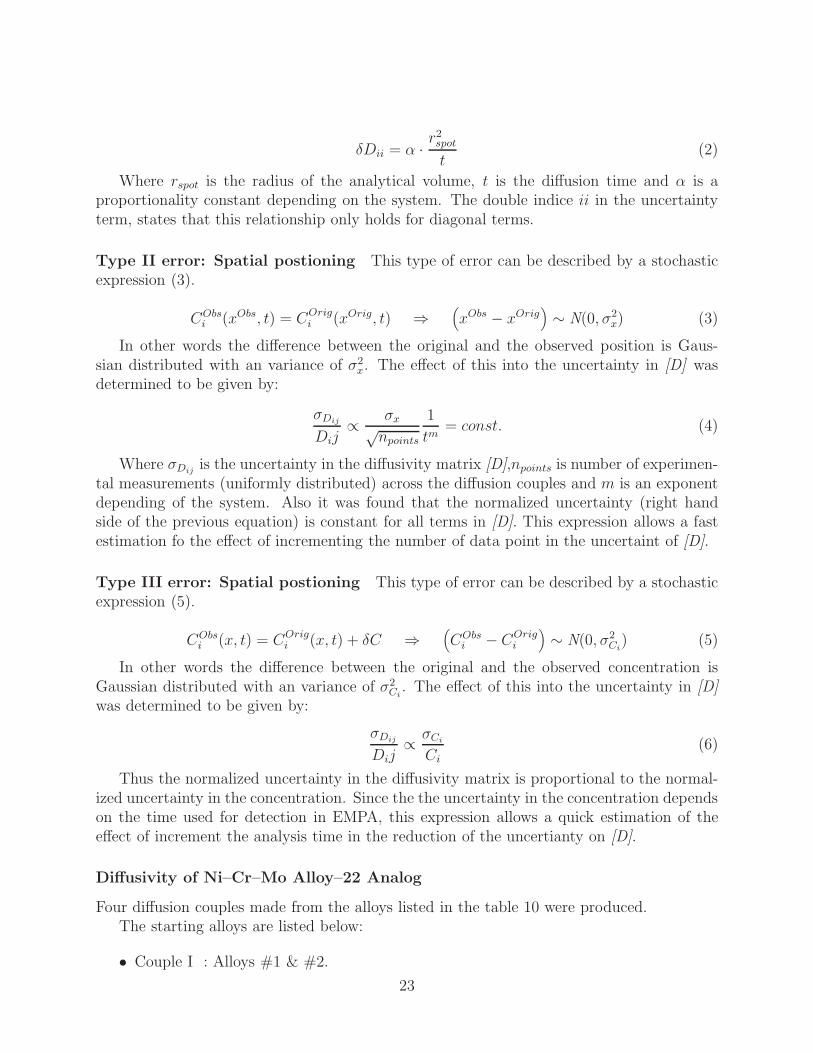
δDii = α · r2spot

t(2)

Where rspot is the radius of the analytical volume, t is the diffusion time and α is aproportionality constant depending on the system. The double indice ii in the uncertaintyterm, states that this relationship only holds for diagonal terms.

Type II error: Spatial postioning This type of error can be described by a stochasticexpression (3).

CObsi (xObs, t) = COrig

i (xOrig, t) ⇒(xObs − xOrig

)∼ N(0, σ2

x) (3)

In other words the difference between the original and the observed position is Gaus-sian distributed with an variance of σ2

x. The effect of this into the uncertainty in [D] wasdetermined to be given by:

σDij

Dij∝ σx√

npoints

1

tm= const. (4)

Where σDijis the uncertainty in the diffusivity matrix [D],npoints is number of experimen-

tal measurements (uniformly distributed) across the diffusion couples and m is an exponentdepending of the system. Also it was found that the normalized uncertainty (right handside of the previous equation) is constant for all terms in [D]. This expression allows a fastestimation fo the effect of incrementing the number of data point in the uncertaint of [D].

Type III error: Spatial postioning This type of error can be described by a stochasticexpression (5).

CObsi (x, t) = COrig

i (x, t) + δC ⇒(CObs

i − COrigi

)∼ N(0, σ2

Ci) (5)

In other words the difference between the original and the observed concentration isGaussian distributed with an variance of σ2

Ci. The effect of this into the uncertainty in [D]

was determined to be given by:

σDij

Dij∝ σCi

Ci(6)

Thus the normalized uncertainty in the diffusivity matrix is proportional to the normal-ized uncertainty in the concentration. Since the the uncertainty in the concentration dependson the time used for detection in EMPA, this expression allows a quick estimation of theeffect of increment the analysis time in the reduction of the uncertianty on [D].

Diffusivity of Ni–Cr–Mo Alloy–22 Analog

Four diffusion couples made from the alloys listed in the table 10 were produced.The starting alloys are listed below:

• Couple I : Alloys #1 & #2.

23

Table 10: Alloys composition in % wt

Alloy# Weight %Ni Cr Mo

1 66.0 20.2 14.02 72.1 15.1 12.83 67.7 15.7 16.64 72.9 17.4 9.75 69.7 21.2 9.16 64.3 24.3 11.4

• Couple II : Alloys #1 & #3.

• Couple III: Alloys #1 & #4.

• Couple IV: Alloys #1 & #2.

The diffusion couples were annealed for 48 hours at 1215 ± 5 ◦C.From each diffusion couple, two EPMA line scans were produced. In the tables 11, 12, 13,

and 14, are presented the measured composition from each line scan.Since the method implemented here to find the diffusivity matrix [D] requires the con-

centration profile for two diffusion couples, the data obtained was grouped in the followingcases:

• Case A: Couple I, Line scan #1; & Couple II, Line scan #1.

• Case B: Couple I, Line scan #2; & Couple II, Line scan #2.

• Case C: Couple IV, Line scan #1; & Couple III, Line scan #1.

• Case D: Couple IV, Line scan #2; & Couple III, Line scan #2.

The diffusivity and the square root diffusivity matrix and their eigenvalues consideringMo as base element were determined from each case. The results, including the eigenvaluesfor the matrices, are presented in the tables 15 and 16.

Table 11: End compositions for diffusion couples I, in %at

Couple ILine scan # 1 Line scan # 2

C−i C+

i C−i C+

i

Nickel 67.0 73.3 67.1 73.3Chromium 24.6 18.6 24.7 18.6Molybdenum 8.3 8.0 8.3 8.0

24

Table 12: End compositions for diffusion couples II, in %at

Couple IILine scan # 1 Line scan # 2

C−i C+

i C−i C+

i

Nickel 67.1 70.0 67.0 69.9Chromium 24.7 19.8 24.7 19.8Molybdenum 8.2 10.2 8.2 10.2

Table 13: End compositions for diffusion couples III, in %at

Couple IIILine scan # 1 Line scan # 2

C−i C+

i C−i C+

i

Nickel 68.1 74.0 68.1 74.0Chromium 23.8 20.4 23.9 20.4Molybdenum 8.1 5.6 8.1 5.6

Table 14: End compositions for diffusion couples IV, in %at

Couple IVLine scan # 1 Line scan # 2

C−i C+

i C−i C+

i

Nickel 68.0 74.1 68.0 74.2Chromium 23.8 18.0 23.9 17.9Molybdenum 8.2 7.9 8.2 7.9

Table 15: Diffusivity Matrix: Diffusion Couples at 1215 ◦C. All the values are in 10−10[cm2/s

][D] Case A Case B Case C CaseD

DMoNiNi 4.26 3.84 5.68 4.37

DMoNiCr 0.228 0.199 1.96 0.382

DMoCrNi -1.64 -1.181 -2.82 -1.95

DMoCrCr 2.05 2.20 0.485 1.59E1 4.08 3.68 4.18 4.07E2 2.23 2.36 1.98 1.89

25

Table 16: Sq. Root Diffusivity Matrix: Diffusion Couples at 1215 ◦C. All the values are in10−5

[cm2/s

][r] Case A Case B Case C CaseD

rMoNiNi 2.07 1.96 2.48 2.10

rMoNiCr .0650 .0576 .568 .113

rMoCrNi -.466 -.342 -.817 -.576

rMoCrCr 1.44 1.49 0.975 1.29e1 2.02 1.92 2.04 2.02e2 1.49 1.54 1.41 1.37

From the previous results, we obtained the average for the elements in the square rootdiffusivity matrix. This value was used as the starting point for the global fitting. Thediffusivity matrix and the square diffusivity matrix obtained from the global fitting arepresented below for the different elements (Mo, Ni, Cr) as base element.

[DMo

NiNi DMoNiCr

DMoCrNi DMo

CrCr

]=

[4.60 0.681

−1.87 1.70

]· 10−10

[cm2/s

][

DNiCrCr DNi

CrMo

DNiMoCr DNi

MoMo

]=

[3.57 1.87

0.349 2.73

]· 10−10

[cm2/s

][

DCrMoMo DCr

MoNi

DCrNiMo DCr

NiNi

]=

[2.38 −0.349

−0.680 2.73

]· 10−10

[cm2/s

][

rMoNiNi rMo

NiCr

rMoCrNi rMo

CrCr

]=

[2.17 0.194

−0.533 1.34

]· 10−5

[cm/

√s]

[rNiCrCr rNi

CrMo

rNiMoCr rNi

MoMo

]=

[1.88 0.533

0.0993 1.64

]· 10−5

[cm/

√s]

[rCrMoMo rCr

MoNi

rCrNiMo rCr

NiNi

]=

[1.54 −0.0993

−0.194 1.98

]· 10−5

[cm/

√s]

The results presented above were used with the end compositions to generate the cal-culated concentration profile for each case. The experimental and calculated concentrationprofiles are presented in Figures 12 and 13. In addition, the experimental and calculateddiffusion profile for all cases in the composition space (Cr,Mo at%) are shown in figure 14 .

As additional comment, in the EPMA analysis of the diffusion couples no porosity wasobserved, neither in the original interface or the bulk of the diffusion couple. The imagingin this equipment was generated from secondary electrons with a magnification of 125 X(approx.).

26

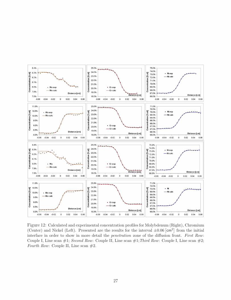
Figure 12: Calculated and experimental concentration profiles for Molybdenum (Right), Chromium(Center) and Nickel (Left). Presented are the results for the interval ±0.06

[cm2

]from the initial

interface in order to show in more detail the penetration zone of the diffusion front. First Row :Couple I, Line scan #1; Second Row : Couple II, Line scan #1;Third Row : Couple I, Line scan #2;Fourth Row : Couple II, Line scan #2.

27

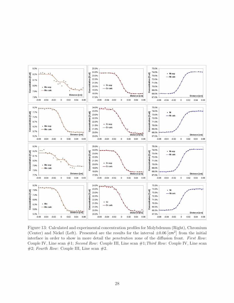
Figure 13: Calculated and experimental concentration profiles for Molybdenum (Right), Chromium(Center) and Nickel (Left). Presented are the results for the interval ±0.06

[cm2

]from the initial

interface in order to show in more detail the penetration zone of the diffusion front. First Row :Couple IV, Line scan #1; Second Row : Couple III, Line scan #1;Third Row : Couple IV, Line scan#2; Fourth Row : Couple III, Line scan #2.

28

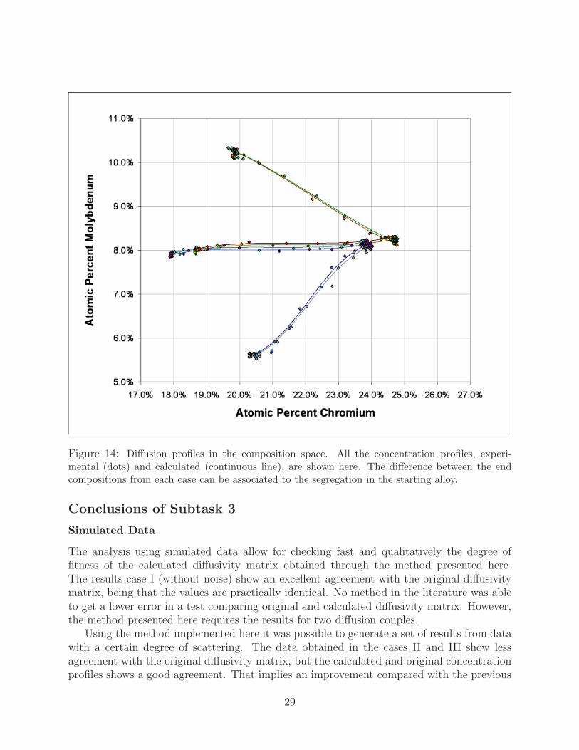
Figure 14: Diffusion profiles in the composition space. All the concentration profiles, experi-mental (dots) and calculated (continuous line), are shown here. The difference between the endcompositions from each case can be associated to the segregation in the starting alloy.

Conclusions of Subtask 3

Simulated Data

The analysis using simulated data allow for checking fast and qualitatively the degree offitness of the calculated diffusivity matrix obtained through the method presented here.The results case I (without noise) show an excellent agreement with the original diffusivitymatrix, being that the values are practically identical. No method in the literature was ableto get a lower error in a test comparing original and calculated diffusivity matrix. However,the method presented here requires the results for two diffusion couples.

Using the method implemented here it was possible to generate a set of results from datawith a certain degree of scattering. The data obtained in the cases II and III show lessagreement with the original diffusivity matrix, but the calculated and original concentrationprofiles shows a good agreement. That implies an improvement compared with the previous

29

methods, since most of them require smooth concentration profiles.The agreement between the original and calculated data for the cases II and III can be

confirmed analyzing the eigenvalues for the calculated diffusivity matrix.From the analytical solution for the diffusion equation the eigenvalues of the square

root diffusivity matrix defines the penetration depth of the diffusion process. Therefore,comparing the eigenvalues could give an idea of how close are the estimated penetration andgeneral shape for the diffusion profile. It confirms that although some of the terms in thecalculated diffusivity matrix differ from the original, the calculated diffusivity matrix is stillable to represent the diffusion phenomena. The maximum difference between the squareroot diffusivity matrix eigenvalues are 14% for Case II and 4% for Case III.

One way to reduce the deviation is to use a high number of experimental data, or morediffusion couples. In the case that the method implemented here is reliable, it is expectedthat the error propagation must decrease with the reduction in the scattering of the originaldata. The analysis using MonteCarlo simulations confirms those statements.

Monte Carlo Simulations

The analysis done using MonteCarlo simulations can be seen as an extension of the resultpresented in the previous section. Considering a large number of simulations allows forgeneralizing the conclusions and reducing the impact of particular results. These resultswere generated using an uniform probability distribution for the error in the concentrationvalue. If a direct representation of the error effect from a specific instrument is required, theuse of a proper probability distribution will lead to more representative results.

The values of the mean and the median are almost coincident enabling to state that theskewness for the data distribution can be neglected. It allows for considering the mean asrepresentative value for the data, and it is a required condition to consider that the valuesfollow a Gaussian distribution. The symmetry on the data distribution and their closenessof the mean for each data set to the original values support that an extensive analysis usingduplicate data would converge in a good approximation to the real value of diffusivity matrix.

An interesting result can be observed in the values of the coefficient of variation (s/x).There is an inverse relationship between the value of the terms in the diffusivity matrix (Dij)and its coefficient of variation. In other words, the smallest values in the diffusivity matrixwill show a higher range of uncertainty. So, the highest value in the diffusivity matrix isbetter estimated than the rest of the values.

The eigenvalues show a different behavior, the smallest eigenvalues show a lower coeffi-cient of variance than the highest one. In addition, the coefficient of variance is ever lowerfor the eigenvalues than the ones for the terms in the diffusivity matrix. Considering thatthe eigenvalues define the penetration depth and the error in the position is negligible, theestimation on the penetration depth is done efficiently.

From the figure 11 it is possible to see that value of the standard deviation goes tozero as the value of the uncertainty in the measured concentration profiles goes to zero.Although those results are only directly applied to the simulated cases, it is possible toanalyze how the reliability of the results is affected as the error in the concentration analysisis increased. Since the experimental results presented here are obtained with an uncertainty

30

in the composition analysis around 1% (for Molybdenum), there it is no guarantee thata good value is obtained for the diffusivity matrix using the results of only two diffusioncouples.

The standard deviation shows a dependence which can be assumed proportional for therange analyzed. This helps to analyze how the reduction in the error on the analysis willaffect the uncertainty in the results. As an example in the case of EPMA analysis theerror could be approximated as the square of the analysis time, since the counting in theinstrument can be associated to a Γ distribution. Therefore, if it is required to reduce theuncertainty in calculated diffusivity matrix by half, it will be required to increment theanalysis time four times.

Diffusion Couple Results

Most of the concentration profiles measured show a smooth “s” shaped curve. Neverthelessthe results for Molybdenum in the Couples I & IV show a high degree of scattering, makingit difficult to identify a concentration profile. It can be explained considering that for thosealloys there is a difference less than 0.5% between the Molybdenum end compositions, so theeffects of the uncertainty in the composition analysis becomes quite relevant.

The differences between the end compositions between the lines scans (less than 0.1%at) for each diffusion couple can be explained considering the uncertainty in the EMPAanalysis. However, the difference for the end compositions (alloy #1 and #2) in the couplesI and II compared with the end compositions for the couples III and IV are much morerelevant, being about 1% of difference (section 14). This effect can be explained from theaxial segregation in the original alloy. Since wafers for the diffusion couples are obtainedfrom the same slug and the alloys was poured in a cylindrical mold, the solute rejection canproduce a concentration profile like the observed here.

The data obtained for the diffusivity matrix from each case (pair of diffusion couples)shows it to be quite close between them, with the exception of the case C. In any case, thecalculated values for [D] are close in order of magnitude to the rest of the results. In orderto consider the results for case C, as an outliner there it is needed to conduct a statisticalevaluation. It will require additional data points for the diffusion couples or reproduction ofthe experimental diffusion couples. The diffusion couples used in case C are the same as incase D, but using different line scans, and both generate relatively different results for thediffusivity matrix.

This fact supports that the results for the terms of the diffusivity matrix are affected bythe error in the concentration analysis. On the other hand, the values for the square rootdiffusivity matrix eigenvalues show a good agreement between each case. It confirms thatalthough the case C produces different results it has the same penetration depth and curveshape as the case D.

In order to answer how a result for [D] with a difference of an order of magnitude forsome of the terms whem compared to the rest of the results could generate similar diffusionprofiles, it is possible to look in detail at the computation of the eigenvalues. From thediffusional analysis theory is possible to see that the eigenvalues are more influenced by thediagonals than the non-diagonals terms in the diffusivity matrix. In addition, the eigenval-

31

ues are more influenced by terms with higher order of magnitude. Both effects combinedallow for dietermining the highest diagonal term in the diffusivity matrix as controlling theuncertainty in the eigenvalues. Also, the impact of the lack of quality in the terms withlower order of magnitude and non diagonal in the prediction of the eigenvalues is reduced.Those observations are confirmed by the results of the case C.

From the results for cases A, B, C, D, there is obtained a global estimate value for thediffusivity matrix using the whole set of data. The degree of representation of those datacan be appreciate in the figures 12 and 13. The calculated values (continuous lines) show agood agreement with the experimental data (symbols). For the results of Molybdenum in theCouples I & IV the calculated profile shows a step in the diffusion profile, corresponding to anear zero gradient zone in the concentration profile. Some agreement can be observed fromthe experimental data. Since it corresponds to a non downhill diffusion case, experimentaldata in previous research also show high scattering in the concentration profile in thosecases [25]. Currently, there is no physical explanation for this behavior in multicomponentdiffusion besides that the error in the instrument could affect the perception of particularfeatures. In the present case it is made worse considering the low difference in the endcompositions.

The zero gradient characteristic in the concentration profile for Mo in the Couples I & IVcould be confirmed analyzing the angle φ in the space composition for this diffusion couple[26, 27]. Reporting the values for a different base element allows for direct calculation ofthe particularities for the system. As an example, it is possible to calculate the compositionangle φ defined by end compositions. In order to produce a zero gradient concentrationprofile (ZG) [26]. Calculating it directly from Cr based square root diffusivity matrix:

φZG = tan−1

(rCrNiNi

rCrMoNi

)= 92.9◦

For comparison purposes, the composition angle φ for the Mo profile in the couple IVfirst line scan is calculated:

φIV = tan−1(

ΔCNi

ΔCMo

)= tan−1

(−6.1

0.3

)= 92.8◦

The values for both angles are almost the same, confirming that for the couple IV a closeto zero gradient concentration profile must be expected. This characteristic is confirmedfrom the concentration profile plots in the figures 12 and 13 showing this detail.

The interval of compositions analyzed in the diffusion couples are in the γ phase of theNi-Cr-Mo system. But, it is required to note that these results do not explore the wholerange of compositions for the γ phase. However, it is possible to consider that for the rangeof composition analyzed the calculated diffusivity matrix is representative for the problem.

Since no porosity was observed at the secondary electron image, it is expected thatthe Kirkendall porosity is not produced in this system. In any case, further observationsusing scanning electron microscopy are required to confirm this fact. In the case that noKirkendall porosity is produced in the system, it will confirm that the changes in the molarvolume through the range of compositions in the diffusion couples are negligible. It is one ofthe requirements that allow to use of constant diffusivities to represent the multicomponentdiffusion.

32

33

General Subtask Conclusions

The inverse problem of finding the diffusivity matrix from experimental data was approached using fitting parameters combined with the analytical results for the diffusion equations. This approach was able to obtain a representative diffusivity matrix from experimental results including data scattering representing the error in the concentration analysis. The use of advance optimization strategies were a suitable technique for the non linear regression presented here. Although the method developed here was applied to a specific system, it can be applied to any system were the diffusivity matrix is expected to be approximately constant and no relevant thermodynamics effects occurs.

The effect of the error in the experimental data affects directly the uncertainty of the calculated value for the diffusivity matrix. However although the values for the terms of the diffusivity matrix Dij can vary in a range from each set of data, the values of the diffusivity matrix eigenvalues tend to be more invariant. It implies that the estimation of the penetration depth in a multicomponent diffusion can be done with a fair level of uncertainty.

The use of MonteCarlo simulations to evaluate the effects of the uncertainty reveals a suitable tool for this problem. It not only allows to estimate the uncertainty in the obtained value. Also it can be used for the estimation of the impact in improvement of the quality analysis (reduction of the error) in the level of confidence in the result obtained for the diffusivity matrix. The multicomponent diffusion in Ni-Mo-Cr for the interval of composition analyzed is effectively represented by constant diffusion coefficients. Although it is possible to shift the element base for [D] through mathematical transformations, it is useful to report them for different base elements. Here having the results for different base elements it allows the direct computation of the composition angle φ required to obtain the zero gradient concentration profile for system with a constant diffusion coefficients. Therefore there is not a direct advantage in selecting the component with the higher concentration as base element, which is done traditionally in the literature. Personnel This cooperative agreement activity directly supported numerous personnel, serving in various roles. A list of participating personnel is below.

1 J.C. LaCombe (PI)

2 L.G. McMillion (Co-PI)

3 S. Namjoshi (Co-Pi)

4 M.E. LaCombe (Staff)

5 A. Manavbasi (Graduate Student)

6 A. Jaques (Graduate Student)

34

7 G. Larios (Graduate Student)

8 S. Vadwalas (Graduate Student)

Dissemination This activity has directly led to numerous technical publications and presentations by the Principal Investigator and the numerous students supported by the grant. Several additional pubications are currently being drafted for publication in the coming year. These are listed below.

Publications:

1 Variational Approach to the Boltzmann Mantano Methods for Determination of the Diffusivity Coefficient IN PREPARATION FOR 2009 SUBMISSION

2 Assessment of Ternary Multicomponent Diffusion in Alloy 22 (Ni-Cr-Mo), Defect and Diffusion Forum, 266, 181-190 (2007) [A.V. Jaques, and J.C. LaCombe].

3 Variation in Susceptibility of Alloy-22 to Localized Corrosion, after Various Heat Treatments, NACE 2007 meeting, (March 2007) [S. Vadwlas, G.M. Larios, M. Taylor, A. Manavbasi, A. Jacques, G. Mcmillion, and J.C. LaCombe].

4 Determination of the Diffusivity Matrix from Experimental Data in Ternary Systems, 2006 SHPE Meeting, New Orleans, LA, (January 2006) [Alonso V. Jacques and Jeffrey C. LaCombe].

5 Effect of Phase stability and Segregation on the Corrosion properties of Alloy-22 (UNS NO6022) in Base metal and Weldments, M.S. Thesis, The University of Nevada, Reno, (December 2007) [S. Vadwalas].

6 Microstructural Characterization of Phase Stability and Variability in Alloy 22, M.S. Thesis, The University of Nevada, Reno, (2007) [G. Larios].

7 Linear multicomponent diffusion in the gamma phase in the Ni-Cr-Mo system, M.S. Thesis, The University of Nevada, Reno, (2007) [A. Jaques].

Presentations:

1 Instrument Error and its Propagation through Diffusion Coefficient Measurement Procedures, MS&T 2008 (Pittsburgh, PA) (October, 2008) [J.C. LaCombe*, A.V. Jaques] INVITED.

2 Uncertainties in Multicomponent Diffusivities and the Determination of Long-Term Diffusivities at Low Temperatures, Diffusion Working Group Meeting (NIST, Gaithersburg, MD) (May, 2008) [J.C. LaCombe*, A.V. Jaques] INVITED.

35

1 Instrument Error Propagation in the Determination of Linear Ternary Multicomponent Diffusion Coefficients, MS&T 2007 (Detroit, MI) (September 2007) [A.V. Jacques*, and J.C. LaCombe]

2 Variation in Susceptibility of Alloy-22 to Localized Corrosion after Various Heat Treatments, MS&T 2007 (Detroit, MI) (September 2007) [S. Vadwlas*, G.M. Larios, M. Taylor, A. Manavbasi, A. Jacques, L.G. Mc Million, and J.C. LaCombe]

3 Scanning electron microscopy (SEM) study of heat treated Alloy 22, Poster, 2007 NACE Meeting (March 2007) [Shatrugna Vadwlas*, Guillermo Larios, Matt Taylor, Alp Manavbasi, Alonso Jacques, Glen Mcmillion, Jeffrey C LaCombe].

4 Assessment of Ternary Multicomponent Diffusion in Alloy 22 (Ni-Cr-Mo), 2007 TMS Annual Meeting, Orlando FL, (February 2007) [A.V. Jaques*, and J.C. LaCombe].

5 Determination of Diffusivity Matrix from Experimental Data in Ternary Systems, 2006 SHPE Meeting, New Orleans, LA, (January 2006) [Alonso V. Jacques*, and Jeffrey C. LaCombe]

Other Conclusions A large portion of the original scope of this project was completed, despite significant budget reductions and funding delays in nearly every year of the project. For the first 3 years, the project was conducted in compliance with the NSHE quality assurance program. Most of our data was formally submitted under this program, although final work on all 3 subtasks was completed only after the project became ”non-QA”. This includes three M.S. thesis documents (Jaques, Larios, and Vadwalas).

At the closure of this activity, the key remaining thoughts on this project are below.

1 Conducting the microstructure and corrosion studies on QA certified welds became prohibitively expensive because of the loss of a QA certified weld supplier. Weld material did exist from various DOE/Bechtel sources, but these materials were not available for our use. This curtailed a good portion of our original scope of work.

2 The annual budget allocations for this project were nearly alwasys delayed and reduced from the original budget. This was a significant hurdle to making continuous progress. Funds arrived very late, necessitating unnatural spending habits (save up ahead of time) that made it difficult to plan and committ to hiring staff and students.

3 There was a significant budget cut in the first year, which was when we had intended to use equipment funds to purchase a major instrument (a backscatter detector for our SEM). This cut left us without the instrument necessary to conduct some of the microstructural characterization, reducing our initial scope of work.

4. Of the three subtasks investigated here, Subtask 3 (which was actually just scopingwork), is still the most important portion of this work deserving future research.Subtasks 1&2 have been studied independently and conclusively by other researchers,but the diffusion work conducted here remains the only experimental work investigatingthe diffusive contribution to long-term phase stability of Alloy-22. Numerical modelsconducted by other researchers [16, 17] makes key assumptions regarding the extrap-olation of high-temperature diffusivity data to the lower repository temperatures. Ibelieve that this warrants better experimental verification.

36

Bibliography

[1] Final Report: Waste Package Materials Performance Peer ReviewPanel, Submitted in response to request of USDOE, Bechtel SAIC Co.http://www.ymp.gov/documents/peer_rev/execsum.htm, 2002.

[2] SUMMERS, T.S.E., WALL, M.A., KUMAR, M., MATHEWS, S.J., and REBAK, R.B.Phase Stability and Mechanical Properties of C-22 Alloy Aged in Temperature Range590 to 760 C for 16,000 Hours, in Scientific Basis for Nuclear Waste ManagementXXII, Materials Research Society Symposium Proceedings Vol. 556, Materials ResearchSociety, 1999, 916-926.

[3] SUMMERS, T.S.E., REBAK, R.B., PALMER, T.A., and CROOK, P. Influence ofThermal Aging on the Mechanical and Corrosion Properties of GTAW welds of AlloyN06022 in Scientific Basis for Nuclear Waste Management XXV, Materials ResearchSociety Symposium Proceedings, Vol. 713, Materials Research Society, 2002, 45-52.

[4] REBAK, R.B., SUMMERS, T.S.E., and CARRANZA, R.M. Mechanical Properties,Microstructure and Corrosion Performance of C-22 Alloy Aged at 260 C to 800 C.in Scientific Basis for Nuclear Waste Management XXIII, Materials Research SocietySymposium Proceedings, Vol. 608, Materials Research Society, 2000, 109-114.

[5] CIESLAK, M.J., HEADLEY, T.J., and JR, A.D.R., The Welding Metallurgy ofHASTELLOY Alloys C-4, C-22, and C-276. Metallurgical Transactions A, 1986. 17(A),p. 2035.

[6] CIESLAK, M.J., KNOROVSKY, G.A., HEADLEY, T.J., and A. D. ROMIG, J., TheUse of New PHACOMP in Understanding the Solidification Microstructure of NickelBase Alloy weld Metal. Metallurgical Transactions A, 1986. 17(A), p. 2107.

[7] OGBORN, J.S., OLSON, D.L., and CIESLAK, M.J., Influence of Solidification on theMicrostructural Evolution of Nickel Base Weld Metal. Materials Science and Engineer-ing, 1995. 203(A), p. 134.

[8] PAN, Y.-M., DUNN, D.S., CRAGNOLINO, G.A., and SRIDHAR, N., Grain-BoundaryChemistry and Intergranular Corrosion in alloy 825. Metallurgical Transactions A, 2000.31(A), p. 1163.

[9] MIYATA, K. and IGARASHI, M., Effect of Ordering on Susceptibility to HydrogenEmbrittlement of a Ni-Base Superalloy. Metallurgical Transactions, 1992. 23(A), p. 953.

37

[10] HEUBNER, U.L., ALTPETER, E., ROCKEL, M.B., and WALLIS, E., ElectrochemicalBehavior and its Relation to Composition and Sensitization of NiCrMo alloys in ASTMG-28 Solution. Corrosion, 1989. 45, p. 249.

[11] RAGHAVAN, M., BERKOWITZ, B.J., and SCANLON, J.C., Metall. Transactions A,1982. 13(A), p. 979.

[12] LOPEZ, N., CID, M., PUIGGALI, M., AZKARATE, I., and PELAYO, A., Applicationof Double Loop Electrochemical Potentiodynamic Reactivation Test to Austenitic andDuplex Stainless Steels. Materials Science and Engineering A, 1997. 229(A), p. 123.

[13] FANG, Z., WU, Y.S., ZHANG, L., and LI, J.Q., Application of the Modified electro-chemical Potentiodynamic Reactivation Method to Evaluate Intergranular Corrosionsusceptibility of Stainless Steels. Corrosion, 1998. 54, p. 339.

[14] HODGE, F.G., Effect of Aging on he Anodic Behavior of Ni-Cr-Mo alloys. Corrosion,1973. 29, p. 375.

[15] HODGE, F.G. and KIRCHNER, R.W., Corrosion, 1976. 32, p. 332.

[16] P. E. A. Turchi, L. Kaufman and Z. K. Liu, Modeling of Ni-Cr-Mo based alloys: Part Iphase stability, CALPHAD, Vol.30, 2006, 70-87.

[17] P. E. A. Turchi, L. Kaufman and Z. K. Liu, ”Modeling of NiCrMo based alloys: PartII Kinetics,” CALPHAD, Vol. 31, 2007,237-248

[18] Hack, H.P.1983. Crevice Corrosion Behavior of Molybdenum-Containing Stainless Steelsin Seawater. Materials Performance, 22, (6), 24-30. Houston, Texas: NACE Interna-tional. TIC: 245826

[19] Kenneth J. Evans, Ahmet Yilmaz, S.Daniel Day, Lana L. Wong, John C.Estill, and RaulB. Rebak Using Electrochemical Methods to Determine Alloy 22s Crevice CorrosionRepassivation Potential Research Summary, High-Radiation Nuclear Waste Disposal.

[20] Hastelloy C-22 Alloy, brochure H-2019 E (Kokomo, IN: Haynes International, 1997).

[21] R.B. Rebak, Corrosion and Environmental Degradation, Volume 2 (Weinheim, Ger-many: Wiley-VCH, 2000), p.69.

[22] R.B. Rebak and P.Crook, Advanced materials and Processes, 157(2) (2000), pp.37-42.

[23] D. D. Gorhe, K. S. Raja, S. A. Namjoshi et al., Electrochemical Methods to DetectSusceptibility of Ni-Cr-Mo-W Alloy 22 to Intergranular Corrosion Metallurgical & Ma-terials Transactions A, Vol. 36A, May 2005.

[24] A.V. Jaques, and J.C. LaCombe, Assessment of Ternary Multicomponent Diffusion inAlloy 22 (Ni-Cr-Mo), Defect and Diffusion Forum, 266, 181-190 (2007).

38

[25] M. S. Thompson, J. E. Morral and A. D. Romig, Metallurgical Transactions A 21A(1990) p. 2679.

[26] M. S. Thompson and J. E. Morral, Acta Metallurgica Vol 34, No 11 (1986) p. 2201.

[27] M. S. Thompson and J. E. Morral, Acta Metallurgica Vol 34, No 2 (1986) p. 339.

39