, o

' CONF-911249--2

DE92 009668

CHARACTERIZATION AND PREDICTION OF SPATIAL VARL4BK/rY OF

UNSATUKATED HYDRAULIC PROPERTIES IN A FIELD SOIL:

LAS CRUCES, NEW MEXICO

by T.-C. Jim Yeh,

Deborah E. Greenholtz,

Department of Hydrology and Water Resources

The University of Arizona

Tucson, Arizona

Maliha S. Nash,

Department of Crop and Soil Sciences

New Mexico State University

Las Cruces, New Me,co

and

P. J. Wierenga

Department of Soil and Water Science

The University of Arizona

Tucson, Arizona

FC-o.-DISCLAIMER

This report was prepared as an account of work sponsored by an agency of the United States r:__; ' : • ,./. _..._. :m_lGovernment. Neither the United States Government nor any agency thereof, nor any of their _ '., '_ :' '._.:'

employees, makes any warranty, express or implied, or assumes any legal liability or responsi- _ '7 :__ _ %'_¢ '_ _"bility for the accuracy, completeness, or usefulness of any information, apparatus, product, orprocess disclosed, or represents that its use would not infringe privately owned rights. Refer-

D cncc heroin _oany spccil_icc_ummcrcialprt_Juci.,prucc_, of sclv_cc5y isadc name, i, adcm_=k,

manufacturer, or otherwise does not necessarily constitute or imply its endorsement, recom-

mendation, or favoring by the United States Government or any agency thereof. The views "_and opinions of authors expressed herein do not necessarily state or reflect those of the

United Starer Governmentorany agency thereof. DIS'TRIBU-I'IOI',4OF ""_m.:.,"_'w,._,,..,_"'"""l_:i",/iEt.,'-f IS UNLI;VilTEtD I

a I

i

ABSTRACT

A 91-m transectwas setup inan irrigatedfieldnearLasCruces,New Mexicotoinvestigate

thespatialvariabilityofunsaturatedsoilproperties.A totalof455 samplingpointswere monitored

alonga gridconsistingof91 stationsplacedi m apartby 5 depthsperstation.Post-irrigationsoil

watertensionand watercontentmeasurementswere recordedover45 daysat 11timeperiods.The

instantaneousprofilemethodwas usedtoestimatetheunsaturatedhydraulicconductivityatthe455

samplingpoints.Fiftysoilsamples were alsotaken foranalyzingsand,silt,and claycontent

distributions.The spatialand temporalvariabilityofsoilwatertensionand watercontentwere

investigatedalongwiththespatialvariabilityofparametersofan unsaturatedhydraulicconductivity

model.Resultsoftheanalysisshow thatspatialvariationinsoilwatertensionand watercontentis

consistentwith the soiltexturespatialvariability.In addition,the spatialdistributionof the

estimatedparametervalueofunsaturatedhydraulicconductivityreflectsthesoiltexturedistribution.

Using the statisticsofthe estimatedhydraulicparametervalues,a stochasticsoilwater

tensionmodel was employedtoreproducethevariabilityofobservedsoilwatertension.Although

many assumptions were made, the resultsof the simulationappear promising.

' nil..... ,n,,', nr_,,1, ,,,,',,nll'IB,_,r,,lli.... II;" I1lllqr_' upr..... ,_,'rn,r,,"' 'rtrr'_ll_"Ifll'"P'II"llltlrllPl"III' " II , m,,,lr''",,lllnlIT,in_fl'l.......

INTRODUCTION

Spatial variability of hydrologic properties of geologic formations has been one of the focuses

of hydrologic research during the last decade. Several large-scale field tracer experiments in saturated

porous media were conducted in tahe past few years and a large amount of data were collected to

investigate effects of spatial variability (e.g., Sudicky, 1986 and Garabedian et al., 1990). Such

carefully collected and extensive field data sets provide the opportunity for testing many theories of

flow and solute transport in field-scale problems. Thus, deficiencies of the theories can be identified

and improved. For exampie, Naff et al. (1988) and Dagan (1989) recognize the difficulty of existing

three-d/mensional macrodispersion theories in reproducing solute plumes at the Borden sand aquifer.

Their discussions lead to many speculations of improvements of the theories (Rehfeldt, 1988; Naff et

al., 1989; Rajaram and Gelhar, 1991).

Although several stochastic theories on the effect of spatial variabili_ on flow _nd solute

transport in porous media under unsaturated conditions have been developed (e.g., Dagan and Bresler,

1_83; Yeh et al., 1985a,b,c; Mantoglou and Gelhar, 1987), only a few large-scale field experiments,

where an adequate number of unsaturated hydraulic properties were collected for testing the

stochastic theories, have been carried out.

The purpose of this paper is two-fold: first, to describe a field-scale infiltration experiment in

a soil, _¢here extensive and detailed hydrologic data were collected and second, to quantitatively assess

a soil-water tension variability theory based on a stochastic approach.

MATERIALS AND METHODS

Experimental Field Site

The extensive data analyzed in this study was collected from an experimental plot at the

,.... ,,

J q

• Leyendecker Plant Science Research Center of New Mexico State University, which is located

appro'_dmately 14 km southwest of Las Cruces, New Mexico. This is a semi-arid region with an

average annual precipitation of 0.23 meters. Rainfall is variable with an average of 52% of the rainfall

occurring in July through September. The average maximum temperature is highest in June at 36

degrees C, and lowest in January at 13 degrees C. There is low relative humidity with an average

Class A pan evaporation of 2.39 meters per year. The water table is approxSmately 3 meters deep.

(Hendrickx et al., 1984). The soil type at the experimental plot is classified as a Glendale clay loam

soil (mixed calcareous thermic family of Typic Torrifluvent) (Hendrickx et al., lfJ86).

The experimental plot, 93 meters long by 3 meters wide had been prepared for prior

experiments by disking in two directions, rototilling to a depth of 0.2 meters, and then levelling using

a laser plane. Th(_ plot was further smoothed and levelled by hand and enclosed with a 50-centimeter

raised soil berm (Nash, 1984).

Sampling stations were set up on the plot 1 meter apart along a 91-meter transect to obtain

soil water tension and volumetric water content data. A neutron probe access tube was installed at

each station, in the center of the width of the plot, to a depth of 1.5 meters. For each of the 91

stations, five tensiometers were installed across the width of the plot (0.3 meters apart) with their tips

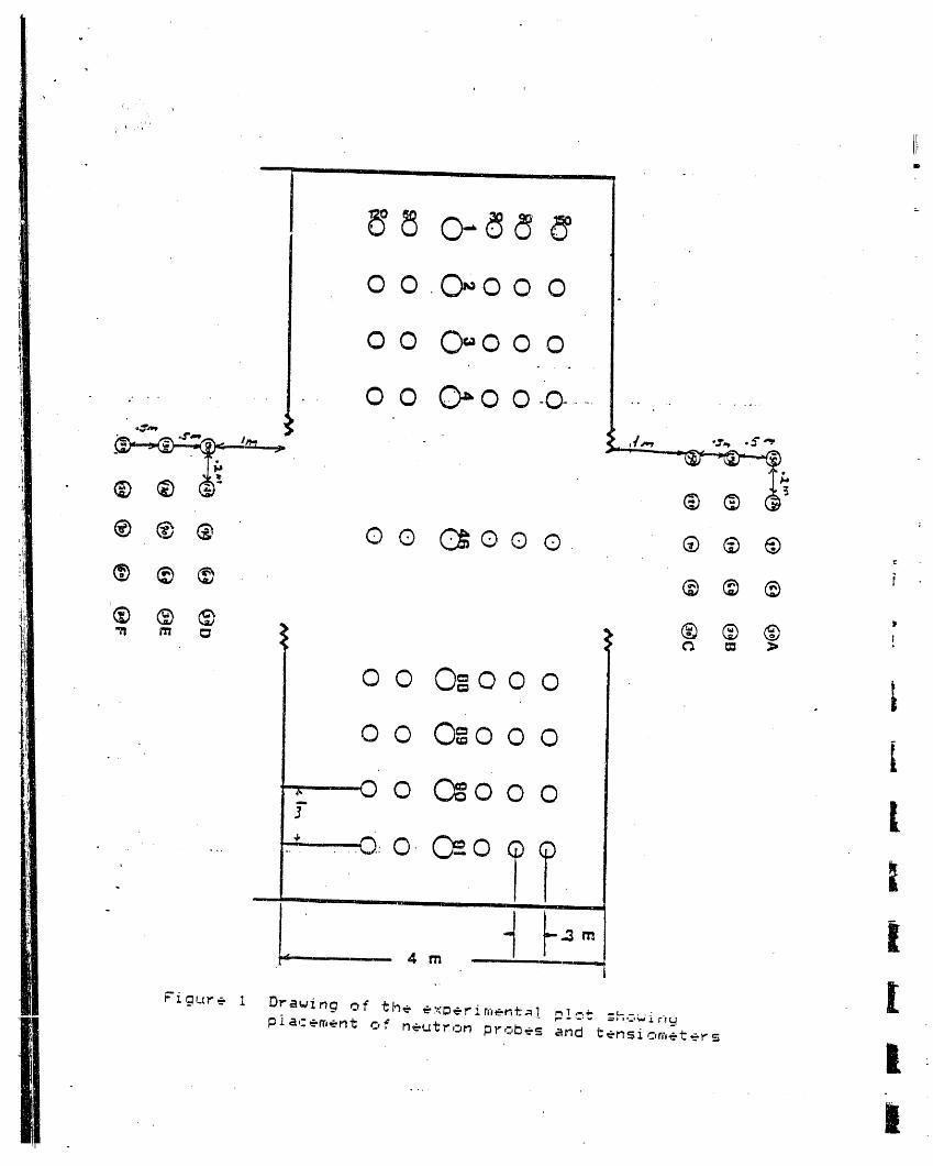
at 0.3, 0.6, 0.9, 1.2 and 1.5 meters. A drawing of the experimental plot showing placement of the

measuring instruments is provided in Figure 1. Although the five tensiometers associated with each

of the 91 stations are not located at the exact site of the access tube, the practical assumption is made

that there are only 455 distinct sampling points for measuring soil water content or tension; 9I

stations by _5depths per station. This experimental set-up and the corresponding assumption are based

on a standard procedure for measuring soil hydraulic characteristics as described by Hillel et al.

(1972). The method requires that a series of tensiometers be installed near the access tube, not g_-eater

than 0.3 meters apart and to a depth as great as possible. The tensiometers must be far enough away

from the access tube to avoid interfering with t,he neutron readings (approximately 0.5 meters), yet

near enough to monitor the "same" soil mass (Hillel et al., 1972). Nash et al. (1989) maintained that

in this particular clay loam soil, the 0.3 meter separation distance is adequate to prevent interference

!I............ ' ....... 'I_.... I""l" I'IFI I ' llir ,,....... ,I ................ n ,_I ........ "ii _, ..... ' IIIll 'lll III,, ,f l"I........... I'l_ I_l TMII I ...... l'II' II'I!I: '' 'r'n'n _'' Tl!lI "fill IFIr Illl I 'IllI_'llI_l iIl_l!_ 'I_ "rollr m_l_,%,ii:_iIIII_ rI_ I_IIfI_Ir'_ _rII_I IIeeII (II_ IIIIT_

. with neutron probe readings.

Fifty soil samples were taken along the transect at five depths at locations 1, 11, 21, 31, 41,

52, 61, 71, 81, and 91. Sand, silt, and clay contents were determined for these soil samples, using the

hydrometer method (Gee and Bauder, 1982).

Volumetric water content was monitored with a neutron probe and moisture meter (CPN

Corporation, Howe Road, Martinez, CA, Model 503DR Hydroprobe). As described above, the neutron

p'robe access tubes had been installed vertically into the soil to a depth of 1.5 meters at each of the

91 stations. The neutron probe was lowered into the access tube, and water content readings were

collected using standard procedure.

Each actual water content measurement is calculated from the neutron moisture meter reading

plus a previously determined calibration curve. The calibration curve plots the relationship between

neutron count rate and volumetric water content. The calibration cllrve is: i = 0.1744 + (Relative

Count Ratio) - 0.0347 with 95% confidence limit intervals for an individual predicted value. One

calibration curve was used for all sampling locations and soil depths.

Soil water tension was monitored with a system consisting 'ofthe 455 installed tensiometers

(91 stations by 5 tensiometers per station), and a hand-held pressure transducer with attached

hypodermic needle and digital-readout device (Soil Measurement Systems, ','344 North Oracle Road,

Tucson, Arizona). This _]'stem is based on the design by Marthaler et al. (1983). The needle is injected

through a rubber stopper sealing the top of each tensiometer, and the tension measurement is

displayed on the readout device. This process can be repeated relatively rapidly until all tension

readings have been recorded.

Each tensiometer was made from a porous ceramic cup (5/8 inch outside diameter), PVC pipe

(0.5 inch schedule 80), clear plastic tubing (0.5 inch internal diameter; 0.625-inch outside diameter)

and a rubber septum stopper. Epoxy Epocast Hardener was used to join the components. The

tensiometer was filled with de-aired water leaving only a small volume of air at the top of the

tensiometer. After each insertion of the needle, silicon rubber cement was reapplied to the rubber

stopper to prevent air le,_age.

• Before installation of the tensiometers in the experimental plot, each was tested for leakage

by submerging it under water and applying up to 1.5 bars of positive pressure. The appearance of

bubbles would indicate leakage. The functior._ing tensiometers were then positioned into holes prepared

with a coring tool. Each tensiometer was installed so that 5 centimeters of plastic tubing and rubber

septum were aboveground. Before taking measurements, the tensiometers were left to equilibrate with

the soil water.

With the tensiometers in place, measurements were taken at the observation times by

insertion of the hypodermic needle into the septum stoppers. Readings were recorded directly from the

digital read-out device, calibrated in millibars. Then soil water tension values were calculated by

subtracting the stem length of the tensiometer from the reading on the meter, in mb or centimeters

water.

A drip irrigation system consisting of 12 irrigation lines laid along the length of the plot was

installed. Both spacing of the tubes and spacing of drip holes in the tubing was approximately 6

inches. The plot was covered with plastic sheeting to prevent evaporation, and a thin layer of soil to

keep the sheeting in place and reduce temperature fluctuations and condensation.

Data were collected at varying irrigation rates in an effort to find the proper rate for reaching

steady-state unsaturated flow. Irrigation was not continuous. One-hour pulses of water were applied

in six cycles a day (beginning at 10:20 a.m., 2:20 p.m., 6:20 p.m., 10:20 p.m., 2:20 a.m., and 6:20 a.m.).

Irrigation began on August 2, 1985 at 1.1 cm/day (900 gal/day). On September 9, the rate was

increased to 2.2 cm/day (1800 gal/day). The final irrigation rate of 4.4 cm/day (3600 gal/day) began on

October 11 and successfully established the desired steady regime. A steady-state system was assumed

when tensiorneter readings remained relatively constant at each location over measured time periods.

Irrigation ceased on November 25, 1985 after nearly four months of irrigation.

Given this experimental set-up, soil water tension and water content values were measured

at each of the 455 sampling stations at 11 different time periods. The times of data collection ranged

bom 5 hours to 44.25 days after irrigation had stopped. The specific 11 measurement periods are: 0.21

days (5 hours), 0.38 days (9 hours), 1.17, 1.42, 2.25, 3.25, 4.25, 7.25, 11.25, 18.25, and 44.25 days.

, ,, ,i,,,,, lp ' '_[ rl' ,,P rl TI,, r, ,,,, , *rP_1.... r,_l ,r_'ql IlJ'rl_ "Pl r n, lplFr_ , r,' I' '' rlr, rl,,,

J i

, Data Preparation: Missing and Outl_

The _'ollected water content and soil water tension data sets were reviewed for missing and

anomalous wetness and suction values. Missing and suspect data which may have been caused by

measurement error, calibration error, malfunction and/or limitations of the measuring instruments,

(particularly leaky tensiometers) were discarded before analyses were carried out.

All of the data collected at the first measurement time of 0.21 days (5 hours) were eliminated

from this study due to numerous missing data points and positive pressure measurements. For the

remaining time periods, both missing values and those identified as unreasonable were estimated as

follows• Four hundred fifty five soil moisture charactel_stic curves ( a plot of pairs of @-_ data at

different times at each sampling location) were constructed, using the neutron probe and tensimeter

data. By a visual inspection of the characteristic curves, anomalous values could be identified. Given

the water content versus tension relationship for each sampling location, the unreasonable and

missing values were then estimated by computer-assisted curve-fitting and/or with a French curve.

A second approach using geostatistics was used to systematically determine unacceptable

values (see Greenholtz et al., 1988). Fitted models to the 50 tension semivariograms were used to

identify the spatial structure for each depth at a specific time period. Then, tensions could be

pinpointed which were _nconsistent with the spatial models. After the validation process using hole-by-

hole suppression, those values found to have standardized errors between the obse_ed and kriged

values greater than a cutoff of 0.9 could be estimated with the kriged value. With 0.9 chosen as the

cutoff value, the validation process eliminated or retained values with roughly the same level of

selectivity as the visual method.

A final determination of whether a value was unreasonable was based on weighing results of

the moisture release curves, the cross-validation of the variogram model, and the level of confidence

in each of these. For instance, if a value had a standardized error greater than 0.9 and was out of line

on the characteristic curve, that value was estimated. If the characteristic curve did not show a clear

relationship, the variogram method for estimation was useful.

,ml=

, i

'DerivationofHydraulicConductivityand Pore-SizeDistributionParameters

Hydraulicconductivityvaluesateachlocationwereestimatedby theinstantaneousprofile

method (Nielsenetal.,1973)usingthewatercontentand soilwatertensionvaluesavailableateach

locationattentimeperiods.Assumingthatthefluxattheplastic-coveredsoilsurfaceiszeroand flow

isone-dimensional,theclassicalinstantaneousprofileformulafordeterminingunsaturatedhydraulic

conductivityis:

_-L[o.I(z)-os(z)]K(o")" (1)

where K is the unsaturated hydraulic conductivity at the center of a layer between two depths of

measurement, _ is the water content, ® is the average water content at the location over a time

interval, t is a time period, and the subscripts represent two different time values, ab/_z is the

change in time-averaged soil water pressure head with depth. The gradient ah/_z is estimated with

a cubic spline function which fits a smooth curve (continuous first derivative) to the average ofthe five

tension values at time t(i+l) and the five values at t(i) (Nielsen et al., 1973). In the derivation process,

the soil surface was treated as having the same water content values as the 0.3-meter depth.

Once the unsaturated hydraulic conductivity values at various moisture contents or suctions

were estimated, the following empirical exponential unsaturated hydraulic conductivity model was fit

to the data:

KCb,)- _ exp(- _ _) (2)

where K is hydraulic conductivity, _ is soil water tension, Ko is hydraulic conductivity parameter at

= 0, and a is the pore-size distribution parameter. When plotted on semilog paper with tension on

the linear x-axis, Kois the intercept and a is the slope.

RESULTS AND DISCUSSION

,I I,Ii, I1'[}

I ii iiii iii l.,l i,,,., lfr ,,,.:..... , I n ii _

J t

'Soil Texture

Figures 2a, b, and c illustrate the spatial distribution of percentage of sand, silt, and clay

content along the profile, respectively. The percentage of sand content throughout the profile increases

with depth with an anomaly near the upper-cen'_er portion of the profile. On the other hand, silt

content tends to decrease with depth. Similar to the silt content distribution, the clay content

decreases with depth. However, soils with high clay colitent values were found near the region

between depths 60-120 cm and locations 41 -81. Statistical analysis of sand, silt, and clay contents

was carried out for data collected at the depth 30 cm (Greenholtz, 1991). However, no statistical

analysis was conducted for the entire soil profile.

Volumetric Water Content Profiles "

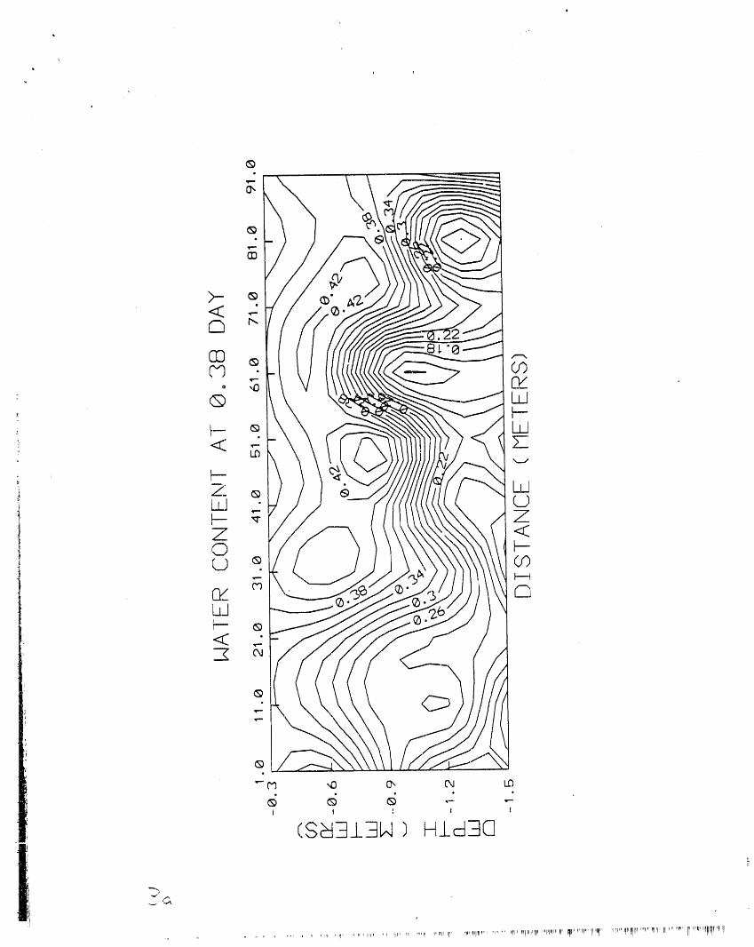
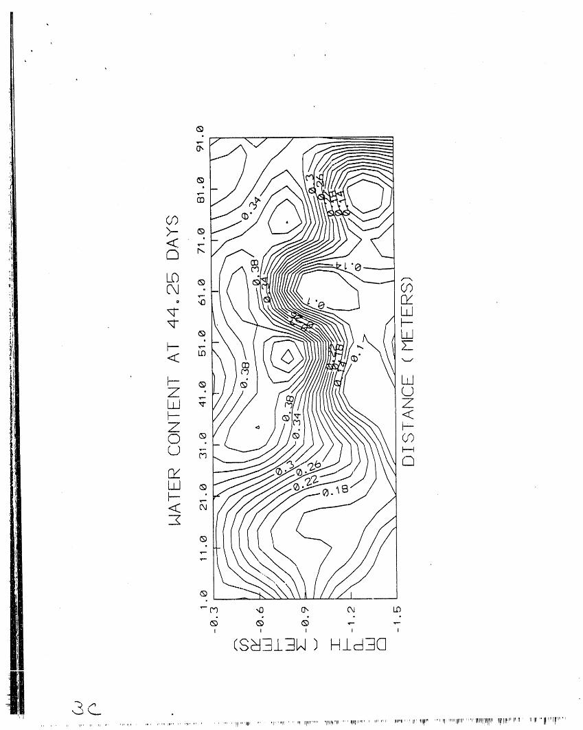
Contour plots constructed for water content for selected times (0.38 days, 11.25 days, and 44.26

days) axe displayed in Figure 3a, b, and c. These plots were made using a contouring progl'am, which

uses the inverse distance squared method to construct the contours. Note that the contour program

smooths contours and deletes extreme values.

In this case krigc _1maps were not made because there were not enough data points to define

an experimental semivariogram for the vel-tical direction, and because of the disparity between

observation intervals along the horizontal and vertical scales. The plots show cross-sections, with the

x-axis corresponding to transect locations, and the y-axis corresponding to depth from 0.3 meters (top

of plot) to 1.5 meters (bottom of plot). Over the time periods, the water content value for any particular

point on the plot decreases. It is e_dent from the plots that the highest water contents are fbund at

the upper depths towards the center of the transect. The lowest water contents are four,Li _t the

lowermost depth, which has greater uniformity of water content values. The most rapid changes in

water content with depth (i.e. plotted lines are clnse together) are found at the middle depths, particu.-

laxly towards the center of the transect. The change to a lower gradient at approximately 1.2 meters

is interpreted as a change in texture. Over time, the contour plots retain the same general shape.

Therefore, the distribution of water content remains similar over the measurement times.

J, I, ,, I,,_I, i ,I .... aBEI[ ,_lJ, , , ii , U JL IIh,lU ,, ,,

r, i

,t

i , J

' Mean Water Contenti *" , i,,, ,,, mi

i Because the soil was observed during drying, a decrease in water content is expected over time.]

:,

Over the observed time periods, the mean water content values do decrease for each depth. These

i means range from 0.382 cmS/cms (at time 0.38 days) for depth 0.6 meters to 0.116 cm3/cm3 (at time_

44.25 days) at the lowest depth. Over the 44 days, the change in mean water content is: 0.069 cm3/cm3

(1.2-meter depth) > 0.060 (0.9-meter depth) > 0.057 (1.5-meter depth) > 0.048 (0.6-meter depth) > 0.033

(0.3-meter depth). Plots of the mean water content values over time for the five depths are shown in

Figure 4. It is evident that the decrease of water content over time is most rapid for the earliest times

sa_r ceasing ofirrigation. The plots then tend to level off (i.e. slowing of the drying rate), particularly

at the upper depths. This slowing of the drying rate may result from the drop in unsaturated

hydraulic conductivity as water content decreases over time.

For any given time period, the highest mean water contents are found at the two uppermost

depths. Thereat_er, water content decreases with depth. The mean water content values at each depth

(averaged over the ten times) follow this same trend of a lowering of water content with depth: 0.363i

i cm3/cm3 (0.6-meter depth) > 0.355 (0.3-meter depth) > 0.284 (0.9-meter depth) > 0.170 (1.2-meter

depth) > 0.153 (1.5-meter depth). From inspection of Figure 4, plots of the mean water content values

over time for the five depths, we again see that the 0.3- and 0.6-meter depths have the highest mean

water contents but seem to level off slightly more than the lower depths over time. This shows more

constant water content values with a slower drying rate at later times. For the lower depths, there

is greater change in water content over time, the drying rate is more rapid, and the drying rate

remains more constant over time.

These results of higher mean water contents at the upper depths and lower mean water

contents at the lower depths associated with more rapid drying are, again, consistent with the soil

texture clam. The lower depths have coarser texture associated with lower retention and more rapid

transnlission of water.

Variation of Water Content

' Plots of variance of water content over time for the five depths are illustrated in Figure 5.

Depths 0.6 and 0.9 meters show a clear increase of variance over the drying period, depth 0.3 meters

levels off aider approximately 11 days, and the lower two depths show a decrease of variance after 8

to 11 days. The middle three depths have higher variance of water content values for any given time

period, and the uppermost and lowermost depths have lower variation. (For all time periods, depth

0.9 meters has the highest variance, and depth 0.3 meters has the lowest.) The depths which exhibit

lower variances (i.e depths 0,3 and 1.5 meters, and to a lesser extent, 1.2 meters) show the most

uniform water content versus location plots across the transect and over the time periods.

At each of the five depths it is found that as mean water content increases, the variance of

water content clearly decreases for the 0.3-, 0.6-, and 0.9-meter depths. No clear trend is evident for

the 1.2-meter depth. For the 1.5-meter depth, there is an apparent increase in variance as water

content increases. The steepest slope (i.e. the greatest change of variance with increased water

content) is found for the 0.6 > 0.9 > 0.3-meter depth.

In order to standardize the variances, coefficients of variation were computed (i.e. standard

deviation divided by the mean). Coefficients of variation are preferable for comparing distributions

with differing means. At all depths, the coefficients of variation for water content clearly increase over

the ten time periods as the soil dries out. Variability of water content ranges from 6-9% in the

uppermost depth to 26-45% in the lower two depths. The increases of the coefficients of variation over

time are consistent with the theory that variability should increase as a soil dries. The slopes for the

two uppermost depths are the least steep and level off more, showing less variability at these depths,

particularly for later times. The 0.3-meter depth, which has a rather uniform water content

distribution along the transect shows low variability and little change over time.

At any given time period, there are higher coefficients of variation with increased depth (with

the exception that depth 1.2 meters had a higher value than depth 1.5 meters). The mean coefficient

of variation averaged over the ten time periods similarly increases with depth ranging from 7% at the

0.3-meter depth to 37% at the 1.2-meter depth. The higher coefficients of variation of water content

found at the lower sandy depths may be related to textural or pore-size differences across the transect.

* v

' Note that the water content versus location plots seem to show less variability for these lower depths.

However, because the mean water content value is much lower for the lower depths, the coefficient

of variation calculated relative to the mean is high.

Figure 6 sh,_ws the plot of the coefficient of variation for water content versus the mean water

content at the five depths. The coefficient of variation for water content increases as the mean water

content decreases. Similar results were also reported by Herkelrath et al., 1991. The slopes for depths

0.6, 0.9, and 1.2 meters are apparently similar. The 1.5-meter depth slope is somewhat less steep, and

the 0.3-meter depth has the least steep slope• Thus, as water content changes, the variation is least

affected for the upper and lower depth.

Histograms were constructed on the raw data for the five depths at each time to visually

inspect the water content frequency distributions. Various degrees of normality are exhibited with

lef_ or right skewness evident in several histograms. Histograms are approximately uniform for the

0.3-me_r depth, tend to be skewed lef_ for the 0.6-meter depth, tend to be bimodal for the 0.9-meter

depth, are skewed right for the 1.2-meter depth, and are approximately normal for the 1.5-meter

depth.

Soil Water Tension

Contour plots of tension for selected times (0.38, 11.25 and 44.25 days) are shown in Figure

7. The plots show cross-sections, with the x-axis corresponding to transect locations, and the y-axis

corresponding to depth from 0.3 meters (top of plot) to 1.5 meters (bottom of plot). Over the time

periods, the tension value for any particular point on the plot increases. The highest tensions are

found towards the ends of the transect. These high tensions are found at the middle depths for time

0.38 days, and extend to the upper-middle depths for the later times. The lowest tensions are found

towards the middle of the transect, and extend from the mid-lower depths at time 0.38 days to the

upper-middle depths at later times. Thus_ the area of lowest tension found in the middle of the

transect shifts from the lower depths to the mid-upper depths over the 44 days. The most rapid

differences in tension values across the transect (i.e. plotted lines are close together) are found

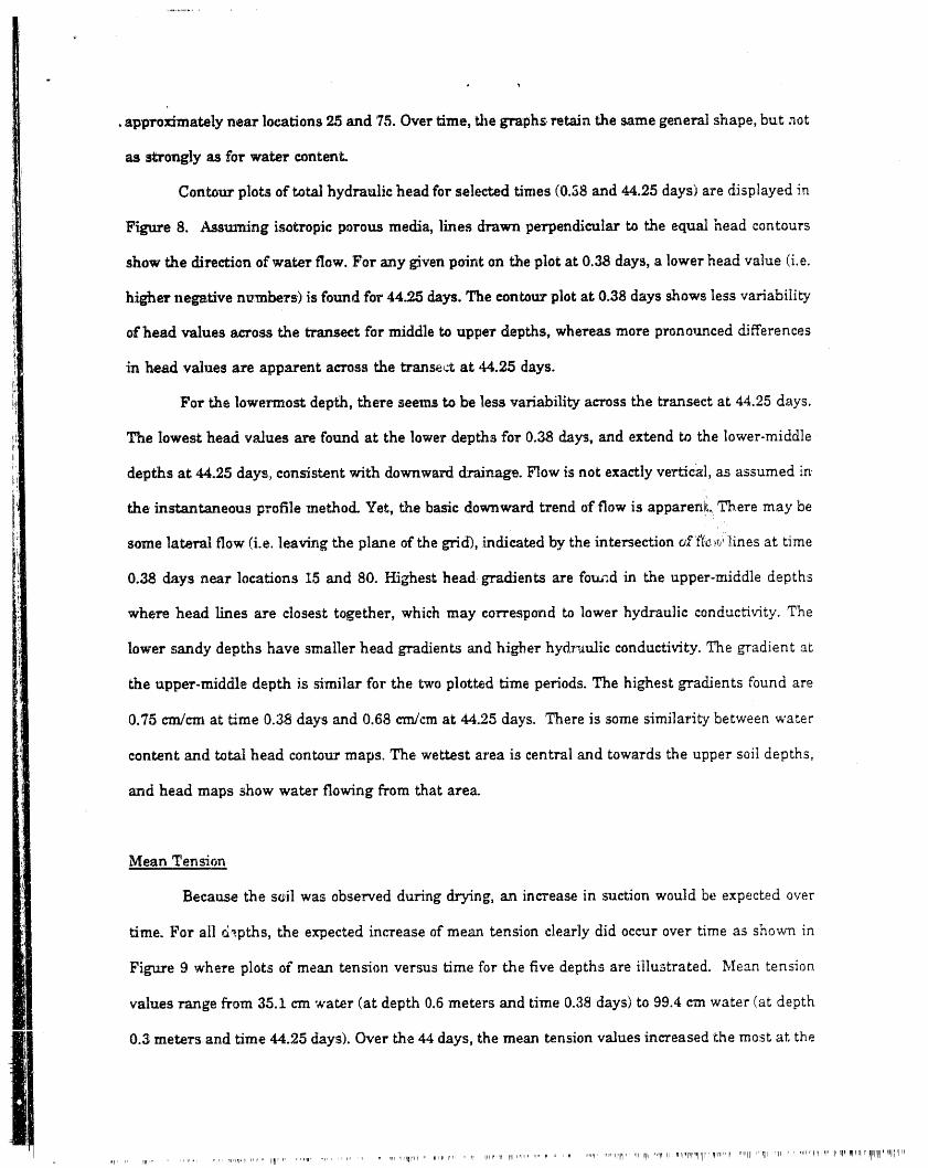
.approximatelynearlocations25 and 75.Overtime,thegraphs,retainthesame generalshape,but not

as stronglyasforwatercontenL

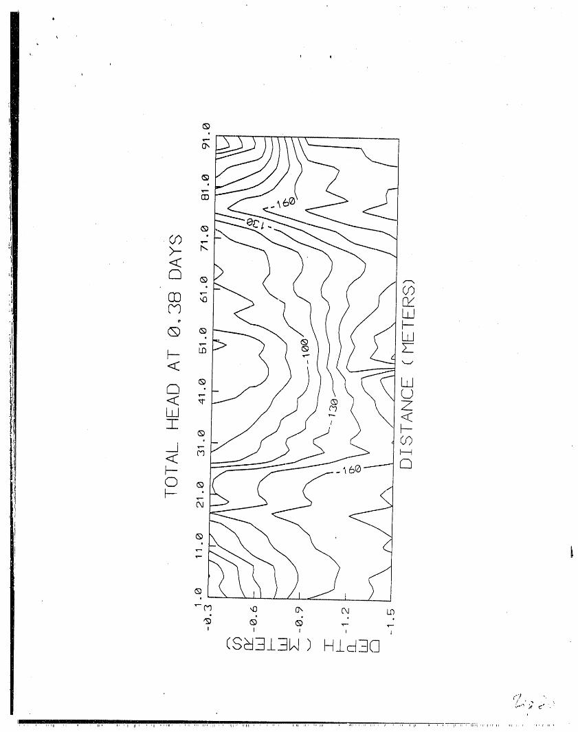
Contourplotsoftotalhydraulicheadforselectedtimes(0.58and 44.25days)aredisplayedin

Figure8. Assuming isotropicporousmedia,linesdrawn perpendiculartot_heequalhead contours

show thedirectionofwaterflow.Forany givenpointon theplotat0.38days,a lowerheadvalue('i.e.

highernegativenvmbers)isfoundfor44,25days.The contourplotat0.38daysshowslessvariability

ofhead valuesacrossthetransectformiddletoupperdepths,whereasmore pronounceddifferences

inhead valuesareapparentacrossthetranse_at44.25days.

For thelowermostdepth,thereseemstobe lessvariabilityacrossthetransectat44.25days.

The lowesthead valuesarefoundatthelowerdepthsfor0.38days,and extendtothelower-middle

depthsat,44.25days,consistentwithdownward drainage.Flowisnotexactlyvertical,asassumed in

theinstantaneousprofilemethod.Yet,thebasicdownward trendofflowisapparen_:Theremay be,

some lateralflow(i.e.leavingtheplaneofthegrid),indicatedby theintersectioncJ__;c_,,iilinesattime

0.38daysnearlocations1,5and 80.Highesthead gradientsarefouledin theupper-middledepths

where head linesare closesttogether,whichmay correspondtolowerhydraulicconduc1:ivity.The

lowersandydepthshave smallerhead gradientsand higherhydraulicconductivity.The gradienta_

theupper-middledepthissimilarforthetwoplottedtimeperiods.The highestgradientsfoundare

0.75cre/creattime0.38daysand 0.68cm/cmat44.25days.Thereissome similaritybetweenwater

contentand totalhead contourmaps.The wettestareaiscentraland towardstheuppersoildepths,

and head maps show waterflowingfromthatarea.

Mean Tension

Because the s_il was observed during drying, an increase in suction would be expected over

time. For all d_pths, the expected increase of mean tension clearly did occur over time as shown in

Figure 9 where plots of mean tension versus time for the five depths are illustrated. Mean tensioa

values range from 35.1 crn water (at depth 0.6 meters and time 0.38 days) to 99.4 cm water (at depth

0.3 meters and time 44.25 days). Over the 44 days, the mean tension values increased the most at the

....r_.... '*'rll'II " _'P'IF_.'."rl II r_'pF.l'",llll ',l'p'll ..,111 .. r;iI .r'll r,f . '"'"q'tlqr' iir I1' _lrllr*llJtll]H' q;llq_'lr_

,upper depthsand theleasta+,thelowerdepths.Specifically,themean changesare62.8(0.3-meter

depth)> 53.1(0.6-meterdepth)> 38.6(0.9-meterdepth)> 30.8(1.2-meterdepth)> 21.4(l.5-meter

depth).In Figure9,theplottedlinesfortheupperdepthsaresteeper,showinga morerapidincrease

ofmean tensionovertime.The plottedlinesforthelowerdepths(particularlyfordepth1.5meters)

arelesssteep,and leveloffovertime(i.e.littlechangeinmean tensionovertime).Therefore,atthe

sandylowerdepth,tensionrapidlyincreasesai_r ceasingofirrigation,but laterremainsnearly

constantovertime.Water_assesthroughthiscoarse-texturedlayer,whichhashighhydraulicconduc-

tjvit3rand low retentionofwater.Thissame resultwas reportedby Nash (1984)onthesam_,soilin

a floodedplotexperiment.

Mean tensiontrendswithdeptharenotclear,butdependon thegiventimeperiod(Figure

9).At earlytimes,themid tolowerdepthstendtohavethehigheJttensions.At latertimes,theupper

tomid depthshavethehighesttensions.The followingtrendisfoundforthefivemean tensionvalues

(averagedoverthetentimes):66.01crn(1.2-meterdepth)> 65 95(0.9-meterdepth)> 64.69(0.3-meter

depth)> 55.97(0.6-meterdepth)> 52.36(1,.5-meterdepth).

Variation of Tension

In the past most researchers have found greater variation of soil water tension and water

content as a soil dries. As seen in Figure 10, an increase of tension variance over time is demonstrated

for depths 0.3 and 0.6 m; the lower depths suggest a relatively constant or possibly decreasing trend.

&s evident in the graphs, the lower three depths exhibit little change in variance over time.

The highest variance for any given time is found at depth 0.6 meters > 0.9 meters > 0.3 meters

> 1.2 meters > 1.5 meters. Depths 1.2 and 1.5 •meters, which are uniformly sanrly, have the lowest

variances. As evident in this plot, variances at the lower three depths remain relatively constant over

time. For depths 0.3 and 0.6 meters, there is a greater change in variance as the soil dries. These

depths have higher percentages of silt and clay than the lower depths (]_gure 2a, b, and c).

A plot of the variance of tension versus mean soil water tension for each of the five depths

shows, that. as the mean soil water tension increases, the variance of soil water tension generally

.

.......... ,T ,_,......... ,........ ' ,,,,,r' "'rP" ,.",i'l' ",_,'li' ,i, a,m,a'r,,lp',_'ap"'IQ_,I, IttpI...... I_aH , ' _ ..... _' "PII_I_at'..... "lr Sill'I' 'qr' llri rllll!'lll_lI, '"rlalrn lalIRW_'lrlQI,r' ' _,',,_l,lllq',lllp_l'lN'_q"_,qpTi,r ,, _111alplr i_,,

q ,

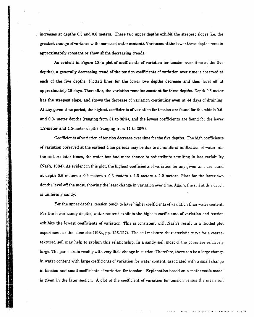
. increasesatdepths0.3and 0.6 meters.These two upperdepthsexhibitthesteepestslopes(i.e.the

greatestchangeofvariancewithincreasedwatercontent).Variancesatthelowerthreedepthsremain

approximatelyconstantorshow slightdecreasingtrends.

As evidentinFigure10 (aplotofcoefficientsofvariationfortensionovertimeatthefive

depths),a generallydecreasingtrendofthetensioncoefficientsofvariationovertimeisobservedat

each of the fivedepths.Plottedlinesforthe lowertwo depthsdecreaseand then leveloffat

approx/mately18 days.Thereafter,thevariationremainsconstantforthesedepths.Depth0.6meter

has the steepestslope,and showsthedecreaseofvariationcontinuingeven at44 daysofdraining.

At anygiventimeperiod,the'highestcoefficientsofvariationfortensionarefoundforthemiddle0.6-

and 0.9-meter depths(rangingfrom 31 to98%),and thelowestcoefficientsare"foundforthelower

1.2-meterand 1.5-meterdepths(rangingfrom 11 to30%).

Coefficientsofvariationoftensiondecreaseover_imeforthefivedepths.The highcoefficients

ofvariationobservedattheearliesttimeperiodsmay be due tononuniforminfiltrationofwaterinto

the soil.At latertimes,thewaterhas had more chancetoredistributeresultinginlessvariability

(Nash,1984).As evidentinthisplot,thehighestcoefficientsofvariationforany giventimearefound

atdepth 0.6meters> 0.9meters> 0.3meters> 1.5meters> 1.2meters.Plotsforthelowertwo

depthsleveloffthemost,showingtheleastchangeinvariationovertime.Again,thesoilatthisdepth

isuniformlysandy.

Fortheupperdepths,tensiontendstohavehighercoefficientsofvariationthanwatercontent.

For thelowersandydepths,watercontentexhibitsthehighestcoefficientsofvariationand tension

exhibitsthelowestcoeffÉcientsofvariation.ThisisconsistentwithNash'sresultina floodedplot

experimentatthesame site(1984,pp.]26-127).The soilmoisturecharacteristiccurvefora coarse-

texturedsoilmay helptoexplainthisrelationship.In a sandysoil,most ofthepo'resarerelatively

large.The poresdrainreadilywithverylittlechangeinsuction.Therefore,therecanbe alargechange

in water content with large coefficients of variation for water content, associated with a small change

in tension and small coefficients ofvari_tSon for tension, Explanation based on a mathematic model

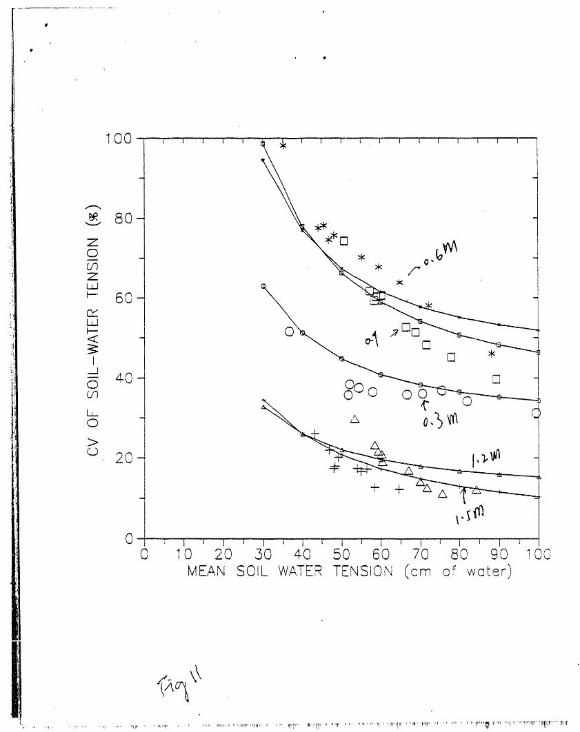
is given in the later section. A plot of the coefficient of variation for tension versus the mean soil

,, ,lr ,...... r 'Pr r'l'llr ........... rll "lllllll"r .... _r..... _q¢'lW, II_'¢l'_l'"" '11' ""llI'llq_Jl

, i

water tension is displayed in Figure 11.

Shapes of histograms constructed on the raw data varied with time and depth. Both right and

left skewness was present. Histograms are skewed right for the 0.3-meter and 0.6-meter depth, skewed

leftorpossiblybimodalforthe0.9-meterdepth,approximatelynormalforthe1.2-meterdepth,and

skewed leftforthe 1.5-meterdepth.

HydraulicConductivityParameters:Kn _nd a

As describedearlier,hydraulicconductivity(Ko)and pore-sizedistributionparameter(a)were

derivedfroma linearregressionofnaturallogofunsaturatedhydraulicconductivityon tensionusing

theexponentialunsaturatedhydraulicconductivitymodel(Eq.2).As a result,themodelmay not

•r_presenttheactualK-_ relationshipofsome soilsovertheentirerangeof_ values,but therange

where themodel isfitted.Inthisfieldexperiment,most of0 and _ datacollectedfallina rangeof

tensionsfrom30 to100cm ofwater,ltislikelythattheestimatedKo may notcorrespondtoactual

saturatedhydraulicconductivityvaluesofthesoilbuttheinterceptextrapolatingfromthelinearInK-

modelfittedtotherangeof_ values.Similarly,theestimateda valuesmay notrepresenttherate

ofreductioninK overtheentirerangeof_ values.Consequently,thederivedK oand ctvalueswere

foundtohave excessivelylargemeans,variances,and coefficientsofvariationateachdepth(Table

1). The horizontalcorrelationscalesresultingfrom variogramanalysesofthedataofKoare5,16,

35,7,and 5metersfordepths0.3,0.6,0.9,1.2,and 1.5meters,respectively.The correspondingvalues

forthea parameteratthesedepthsare6,10,8,11,and 5 meters(Greenhlotz,1990).

ContourplotsofKoand a distributior,,sareillustratedinFigures12a andb,respectively.The

highesta valuesarefoundat thelowerdepthson theends ofthetransect,particularlyat high-

numbered locations.Thesearethesame areaswhere thehighestKovaluesarefound.The general

increaseofI_ and a valueswithdepthisconsistentwiththechangetocoarsertexturewithdepth(see

Figures2a,b,arldc).

StochasticModel

1 ............................ , ..... rl, _ ........... "111' I1 " ==z, Irff '" rl_ll,,r=,,ll .... ill ,i , lr, II_l_'l'l",""l!l'rlIIIl'l'l_ Hr,qll_'IlIIr'll " Ilmllll_il''

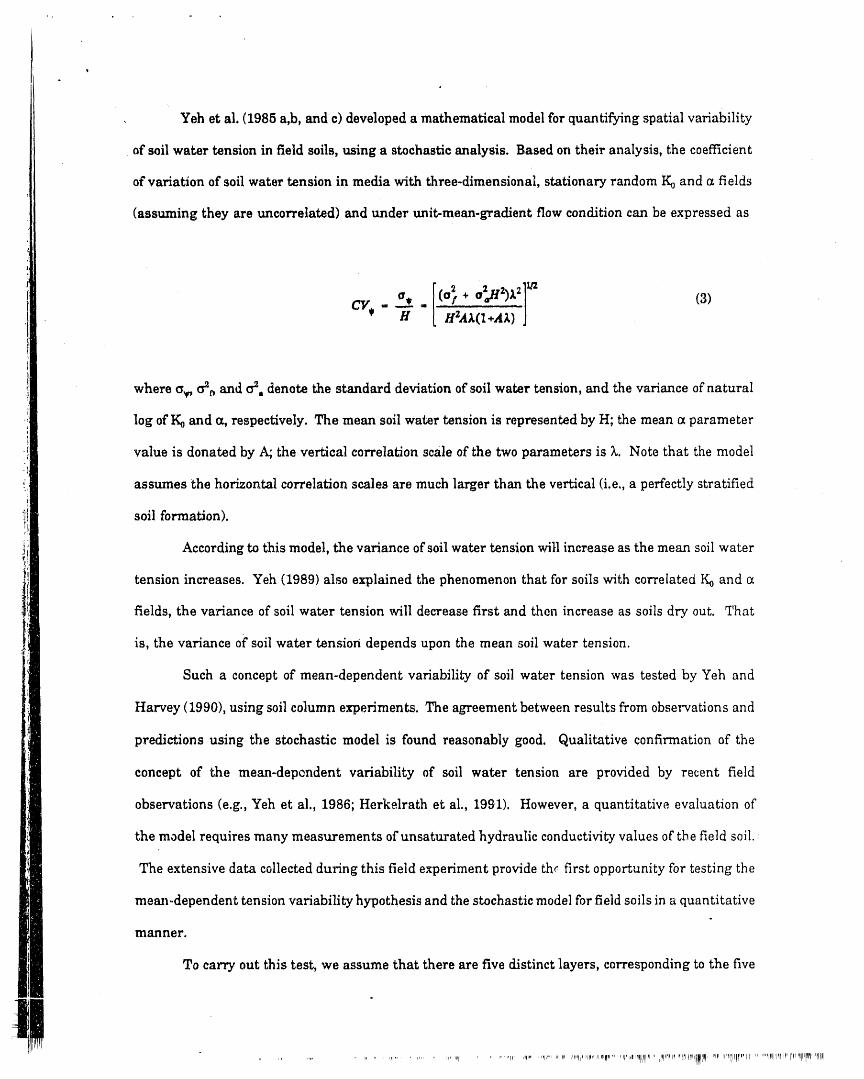
Yeh et al. (1985 a,b, and c) developed a mathematical model for quantifying spatial variability

of soil water tension in field soils, using a stochastic analysis. Based on their analysis, the coefficientr

of variation of soil water tension in media with three-dimensional, stationary random IQ and a fields

(assuming they are uncorrelated) and under unit-mean-gradient flow condition can be expressed as

. (3)

where _v, °_ and ¢_odenote the standard deviation of soil water tension, and the variance of natural

log of Ko and a, respectively. The mean soil water tension is represented by H; the mean a parameter

value is donated by A; the vertical correlathon scale of the two parameters is ;_. Note that the model

assumes the horizontal correlation scales are much larger than the vertical (i.e,, a perfectly stratified

soil formation).

According to this model, the variance of soil water tension _ri)l increase as the mean soil water

tension increases. Yeh (1989) also explained the phenomenon that for soils with correlated Ko and a

fields, the variance of soil water tension will decrease first and then increase as soils dry. out. That

is, the variance of soil water tension depends upon the mean soil water tension.

Such a concept of mean-dependent variability of soil water tension was tested by Yeh and

Harvey (1990), using soil column experiments. The agreement between results from obseTTations and

predictions using the stochastic model is found reasonably good. Qualitative confirmation of the

concept of the mean-depondent variability of soil water tension are provided by recent field

observations (e.g., Yeh et al., 1986; Herkelrath et al., 1991). However, a quantitative evaluation of

the model requires many measurements of unsaturated hydraulic conductivity values of the field soil.

The extensive data collected during this field experiment provide th_ first opportunity for testing the

mean-dependent tension variability hypothesis and the stochastic model for field soils in a quantitative°

manner.

To carry out this test, we assume that there are five distinct layers, corresponding to the five

tl "............. ,i ................ I' ' .... (l_ ,_..... Irl' ,,. r_,,?f,,,I,p, II,vn." ',u_,J,_)_llIIl?j ' II'Illl, l_"l_)l',f_'l_, a)l, Ii,'i,llglf. II ........ l_lll"l_lp' I])i'MlqPI!IUr!llll(

Q i

, deptl_s, In addition, mean soil water tension within each layer ::aring each sampling time is assumed

to be uniform over the thickness of the layer and the flow is steady. With these assumptions, Table

1 provides all the parameter values required for the model, except the vertical correlation scale due

to insufficient number of samples in the vertical direction. To _rcumvent the difficulty in obtaining

the vq_rtical correlation scale, the stochastic model (Eq. 3) was fitted to the observed data by adjusting

the value of the vertical correlation scale. Figure 11 shows the fitted theoretical and observed CV and

H relationships. The vertical correlation scales determined from the best-fit stochastic model are

0.024, 0.087, 0.02, 0.0017, and 0.0021 meters for depths 0.3, 0.6, 0.9, 1.2, and 1.5 meters, respectively.

Although the precision of values of the correlation scales can not be verified, the general trend of the

values seems consistent with soil texture data: fine-textured material tends to have a long correlation

scale and coarse-textured material a short correlation scale.

The agreement between the calculated and observed coefficient of variation and mean soil

water tension relationships is reasonably good but we must emphasize the fact that it is a result; of

regression analysis. The predictive capability of the stochastic model still remains unknown.t

However, it is interesting to note that the model predicts the general trend of the relationship ve_,

well. In other words, the model structure, derived from physically correct flow equations, appears

sound, regardles3 of many simplified assumptions used in the derivation.

The stochastic model also provides a way for explaining the phenomenon that the CV of moisture

content increases as the mean water content decreases. If a simple linear relationship is ass:amed for

the moisture release curve of the soil, i.e.,

0 - c_ + d (4)

where 0 is the moisture content. Both 0 and _ are random quantities. In addition, c and d also can

va.ry spatially and thus are taken to be random variables. The mean and variance of 0 can be

approximated by linearizing the c_ t_rm in (4) and ignoring the correlation between _ and c or d.

That is,

J:l •....... []'F I ............ "' [[ 'Iii....... ' ........... Ill] rl,[_......... [,11 I...... "'P'I" ' " Illl ........ ii]Iii?l,,,rPllIil,, r,',a,rlll ,, ,llPH',lfflr'"'" irPl,[, [_l'Ir'_,'n",rnil,rf,,"11" IrVr' 'lr'n"'l$1'lpllllIrl¢_r,1, lr' ,"q I'1 ' FIpIRI"111'" iIHl,qrl,

Q

1

, |

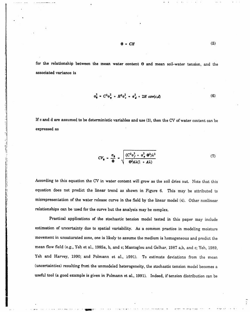
e- c_ (51

b

forthe relationshipbetweenthe mean water contente and mean soil-watertension,and the

associatedvarianceis

If c and d are assumed to be deterministic variables and use (3), then the CV of water content can be

expressed as

iil CVo-°' ¢)z- (7)

Ii According to this equation the CV in water content will grow as the soil dries out. Note that thisequation does not, predict the linear trend as shown in Figure 6. This may be attributed to

misrepresentation of the water release curve in the field by the linear model (4). Other nonlinear

relationshipscan be usedforthecurvebuttheanalysismay be complex.

Practicalapplicationsof the stochastictensionmodel testedin thispaper may include

estimationofuncertaintydue to spatialvariability.As a common practicein modelingmoisture

movement inunsaturatedzone,oneislikelytoassume themedium ishomogeneousand predictthe

mean flowfield(e.g.,Yeh etal.,1985a,b,and c;Mantoglouand Gelhar,1987a,b,and c;Yeh,1989,

Yeh and Harvey, 1990;and Polmann et al.,1991). To estimatedeviationsfrom the mean

(uncertainties)resultingfromtheunmodeledheterogeneity,thestochastictensionmodelbecomesa

usefultool(agoodexampleisgiveninPolmann etal.,1991).Indeed,iftensiondistributioncanbe

,lu_[II r.... lit "'rl ..... _" "'n' Irl' " 'pIll ......

i I lib,

I

,assumed normallydistributed,thisestimateofuncertaintymay providea simpleway toanswera

practicalquestioncommonly raisedby farmers:what percentageofa fieldisunder-irrigatedfora

givenwaterapplicationrate?

Furthermore,unlikeinthesaturatedflow,wherehydraulicheadvariationisrelativelysmall

(Gelhar,1986),thevarianceofsoilwatertensionisgenerallylargeand varieswiththemean tension.

Consequently,thevariabilityoftensioncanbe easilymonitoredwitha largenumber oftensiometers

as demonstratedin thispaper. Ifsome estimatesofthevarianceofInK o and ¢zparametersare

available,thestochastictensionmodel may providea simplymeans toestimatecorrelationscales. .

Obviously,more fieldexperimentsareneededtorigorouslyvalidatethemodeland theapproach.

CONCLUSIONS

Ex*ensive soil Water content and tension data in a soil profile were collected at various time

intervals during drainage. Soil samples were taken for analyzing sand, silt, and clay contents. Soil

water content and tension data were analyzed to investigate the spatial variability. Several

conclusions are drawn from the result of this investigation. They are summarized as follows:

1) In spite of uncertainties in measurements, the general behavior of the observed soil water

content and tension along the profile is consistent with observed soil texture data.

2) The instantaneous profile method for determining unsaturated hydraulic properties seems

adequate to depict the spatial variability of unsaturated soil properties, regardless of its simplicity.

3) Ko and a values obtained by fitting lnK-_ model to K-_ data estimated from the

instantaneous profile method may not reflect accurate saturated hydraulic conductivity values, but

the '])ulk" spatial distributions of both Ko and a values are in a good agreement with soil texture

distributions.

4) Observed spatial variability of soil water content and tension qualitatively supports the

validity of the stochastic tension model developed by Yeh et al. (1985 a,b, and c) although more

carefully planed field expeldments are obviously needed.

ACKNOWI_,DGEMENT

This research is supported by a grant from Ecological Research Division, ER-75, Office of Health &

Environmental Research, Office of Energy Research, Department of Energy under the contract, DE-

FG02-91ER61199.

i

.............. , ,r,_....... ,.... _..... ,_',,ph,'........._' '"111....... _'r,,'_IPPrn"_r'nr_'_"r'ql["'r_ nl'r,'pT,'_,_r,_'r............ _llaV,_,1_,,,l_.... _11n11,I_,I1.....i,lli,rl',....pilllq,,1Hil__F,',,_pn,_111_,'_nlllp'll_li_l,II','l!',r', i'rl 'ni'III,tin'lit'Illn',,r,_r

4

, REFERENCES

Dagan G. and E. Bresler, Unsaturated flow in spatially variable fields, 1, Derivation of models of

infiltration and redistribution, Water Resour. Res., 19(2), 1983.

Dagan, G. Comment on "A note on the recent natural gradient tracer test at the Borden site" by R.L.

Naff, T.-C. J. Yeh, and M. W. Kemblowski, Water Resour. Res., 25(12), 2521-2522, 1989.

Hendrickx, J,M.H., P.J. Wierenga, and M.S. Nash, Variability of soil water tension aud soil water

content. Presented at 1984 Winter Meeting of American Society of Agricultural Engineers, 1984.

;' Hendrickx, J.M.H., P.J. Wierenga, M.S. Nash, and D.R. Nielsen, Boundary location from texture, soil

i.i moisture, and in:filtration data. Soil Sci. Soc. Am. J. 50, 1515-1520, 1986.

Herkeirath, W.N., S.P. Hamburg, and F. Murphy, 'Automatic, real-time monitoring of soil moisture

in a remote fieId area with time domain reflectometry', Water Resour. Res., 27(5), 857-864, 1991.

Hillel, D.V., D. Krentos, and Y. Stylianou, Procedure and test of an internal drainage method for

measuring soil hydraulic characteristics in situ. Soil Sci. 114(5), 395-400, 1972.

Garabedian, S.P., D. R. LeBlanc, L. W. Gelhar, and Michael A. Celia, Large-scale natural gradient

tracer test in sand and gravel, Cape Code, Massachusetts, 2. Analysis of spatial moments for a

nonreactive tracer, Water Resour. Res., 27(5), 911-924, 1991.

Gee G. W. and W. Bauder, Particle-size analysis, A. Klute (ed.), in: Methods of Soil Analysis, Part I,

Physical and mineralogical methods, 2nd edition, ASA Inc. Madision, Wisconsin, p 383-411, 1982.

.... ,........... I, ....... , r, pl,,l]ll ...... Ilmq_ .... II ' "'"' ' II M'IIFFInlIlI,n, ]l'r'll,, ','n'nr'rpll"p,lr_llll !1!11''!iI .... ,,," 'ml'll;_li',,' 11'1_1_1_'11

i

q4

d i

, Gelhar L.W,, Stochastic subsul_ace hydrology from theory to applications, Water Resour. Res., 22(9),

135S-1458, 1986.

Greenholtz, D.E., Spatial variability of hydrologic properties in an irrigated soil, Master's thesis, Dept.

of Hydr. and Water Resour., The Univ. of Arizona, Tucson Arizona, 1990.

Greenholtz, D.E., T.-C. J. Yeh, M. B. Nash, P. J. Wierenga, Geostatistical analysis of soil hydrologic

properties in a field, plot, Jour. of Cont. Hydro., 3, 227-250, 1988.

Mantoglou, A., and L.W' Gelhar, Stochastic modeling of large-scale transient unsaturated flow

systems. Water Resour. Res. 23(1), 37-46, 1987a.

Mantoglou, A., and L.W. Gelhar, Capillary head tension variance, mean soil moisture content, and

effective soil moisture capacity of transient unsaturated flow in stratified soils. Water Resour. Res.

23(1), 47-56, 1987b.

Mantoglou, A., and L.W. Gelhar, Effective hydraulic conductivity of transient unsaturated flow in

stratified soils. Water Resour. Res., 23(1), 57-68, 1987c.

Marthaler, H.P., W. Vogelsanger, F. Richard, and P.J. Wierenga, A pressure transducer for field

tensiometers. Soil Sci. Soc. Am. J. 47, 624-627, 1983.

Naff, R.L., T.-C. J. Yeh, and M. W. Kemblowski, A note on the recent natural gradient tracer test at

the Borden site, Water Resour. Res., 24(12), 2099-2103, 1988.

Naff, R.L., T.-C. J. Yeh, and M.W. Kemblowski, Reply, Water Resour. Res., 25(12), 2523-2525, 1989.

'' ''rlllrl"mll ""' "lllPl "' ''1' ",lIl''u II _

, i

, Nash', M.S.B., Variability in soil water tension, water content and drainage rate along a line transect.

Master's thesis. New MeNco State University, Las Cruces, NM, 1984.

Nash,M.S.,P,J.Wierenga,and A. Butler-Nance,Variationintension,watercontent,and drainage

ratealonga 91-m *-ansect.SoilSci.148(2),944101,1989.

Nielsen, D.R., J.W. Bigger, and K.T. Erh, Spatial variability of field.measured soil-water properties.

Hilgardia. 42(7), 215-259, 1973.

Polmann D. J., D. McLaughlin, S, L. Luis, L. W. Gelhar, L.W. Gelhar, and R. Ababou, Stochastic

modeling of large-scale flow in heterogeneous unsaturated soils, Water Resour. Res., 27(7), 1447-1458,

1991.

Rajaram H. and L. W. Gelhar, _hree-dimensional spatial moments analysis of the Borden tracer test',

Water Resour. Res., 27(6), 1239-1251, 1991.

Rehfeldt, K. R. Prediction of macrodispersivity in heterogeneous aquifers, Ph.D. dissertation, Mass.

Inst. of TechnoL, Cambridge, 1988.

Sudicky, E. A. A natural gradient experiment in a sand aquifer: Spatial variability of hydraulic

conductivity and it_ role in the dispersion process, Water Resour. Res., 22(13), 1447-1458, 1991.

Yeh, T.-C.J., L.W. Gelhar, and A.L. Gutjahr, Stochastic analysis of unsaturated flow in heterogeneous

,_oils. 1. Statistically isotropic media. Water Resour. Res, 21(4), 447-456, 1985a.

Yeh, T.-C.J., L.W. Gelhar, and A.L. Gutjahr, Stochastic analysis of unsaturated flow in heterogeneous

soils. 2. Statistically anisotropic media. Water Resour. Res. 21(4), 457-464, 1985b.

rl,rll""" i]ll' II .... H, , _r m,,, Pqlll" _r,111'4__l_:lr' _I,_' ,11r r'r _111'="' _r',',,,,ll_l_,l,II,I

Q

Yeh, T.-C.J., L.W, Gelhar, and A.L. Gutjahr, Stochastic analysis of unsaturated flow in heterogeneous

soils. 3. Observations and applications. Water Resour. Res. 21(4_, 465-471, 1985c.

Yeh, T.-C.J., L.W. Gelhar, and P.J. Wierenga, Observations of spatial variability of soil-water pressure

in a field soil. Soil Sci. 142(1), 7-12, 1986.

Yeh, T.-C.J., One-dimensional steady state infiltration in heterogeneous soils. Water Resour. Res.

25(10), 2149-2158, 1989.

Yeh, T.-C.J. and D. J. Harvey, Effective hydraulic conductivity of layered sands, Water Resour. Res.,

26(6), 1271-1279, 1990.

i

b

t

Table

Table 1. Means, variances, and coefficients of variations of estimated lnKo and a values at each depth

Figure captions

Figure 1. Drawing of the experimental plot showing placement of neutron probes and tensiometers.

Figure 2. Spatial distribution of percentage of a) sand, b) silt, and c) clay contents along the profile.

Figure 3. Contour plots of water content for a) 0.38 days, b) 11.25 days, and c) 44.25 days.

FigLzre 4. Mean water content over time for the five depths.

Figure 5. Variance of water content over time for the five depths.

Figure 6. Coefficient of variation for water content versus mean water content.

Figure 7. Contour plots of soil-water tension fox'a) 0.38 days, b) 11.25 days, and c) 44.25 days.

Figure 8. Contour plots of total hydraulic head for a) 0.38 days and b) 44.25 days.

Figure 9. Mean soil-water tension over time for the five depths.

Figure 10. Variance of soil-water tension over time for the five depths.

Figure 11. Coefficient of variation for soil-water tension versus mean soil-water tension.

Figure 12. Contour plots of a) natural log of saturated hydraulic conductivity and b) pore-size

distribution parameter.

oo,C_oo o o

oo 0_,o o o

, i

t

Table ," Basic s_atistics for •saturated hydraulic conductivity and pore-size

distribution parameter derived using the final data set

ICSAT ALPHA LNKSAT

DL_)TH 0.3 METERSJ.

MEAN z._E-,,o_ o.oe5 2.29

M_IMUM i _._E.-05 -0.200 - t I. 12

M_aMu'M l.Z4E.o7 o._ 16.nii ,,,,

VARU_CE I.70E*12 0.00_ I1.$8

COEFF. VAR. 8.98E+_'2 7I.S [50.2

_.

DEPTH 0.6 M E'r'ERS

.7; MEAN 5.15E._43,_ 0.0a7 I.66(

-+: MINIMUM 7.63E-0_ 0.0'27 -2.57

:: MAXIMUM 6.09E+06 0.20,1, 15.62":" ST. DEV. 6._6E'_ 0.0¢,0 3.55

""" VARIANCE _,.20E*II 0.002 12._,,_."

.Z_ COE,b_. VAR. 7.93E-W2 45.7 215._

:_:_,7=.

DEFTH 0.9METERS

_ ME.AN 7.,_OE-.,I .I 0.127 5.87--

• MINIMUM 1.67E--01 0.016 -I ./'_

_ MAXIMUM 7. i 0E'_ 15 0.366 36.50

ST.DEY. 7.,1OE.,.i4 0.0_ (_.,_,..-

..-.'L VARIANCE f50E.,.29 0.004 ._1.32

_- 'COEd. VAR. c)a.gE-72 a,c;).5 1099

LDE_'T'I 1.2 METERS._; MEAN I.20E+17 O.14'6 S.35

,-,'_t !MINIMUM 1.49E*00 0.049' 0..'I,0_7 _M_UM 1.10E+_9 0.53l .*3.

¥ sr. oer. _.zoE+t, o.o_ _.9__v_auAN6-: ,._o_._ o.oo_ _.o_

'_ COEFF. VAR. 9.,(,9E.,,_ 48.7 70.9._ )....,...

. _),'tt.#irr

_.- DEPTH 1.5 METERS

MEAN 3.20Eot 7 O. 195 9. II

MINIMU M 2..3] E--Oa O.022 - _. 36

MAXLMU M 2.90E* t9 0.755 al. _ 1

,Sr. DEN. 3.00E+I_ 0.133 8.20

_ANc_ _.o_E._(_ o.o,5_ _7._[cc_'F.v,_. 9_.o'z _.5 _o.o

I K_AT - Saturatedhydraulic conductivityparameter(cmlday)

i ALPHA - Pore-siz_distributionparameter (llcm)LNKSAT =NaturRi log of KSAT

, :..._.: •il ill_l i) "I_" H" _llrl'II III 'IMll' " _rll '"""'ll'i " '"_r Ir",l_ll'"l!11[' "'11 ''ill_l'_l .... I_I_I_I

®

l

I I I I I

(S2±3N) HZd2@

',J ",,._.. .......... Pl[l' 'I_' ...... III....... III.... pl_ll111llr'lllll' _ITIlII_l.l[l ..... [_l_ Ill l_ ....... _ ........ rllllln l l ' lip lllilIIIr.... i111ll,l lllllllllll..... II ll_ll'lllllIlllllllllll_!lllllllI rrll I_ Irl li 111rlllll l' Illii' lll!'ll" ,l

4

®.4@_

Z 8.6 mLd ----.k--" @ 3 mZ0U@,38

@.9 mLL_I

<-T

Z8,2®-<I_.LI2Z 1.2 m

L 1.B m®o18 "l I _ I i-i I I 1 _ I I 'i 1 I' "l---T" I I l L J" I--.....

e _® 2e se 4e seTINE (Days)

,i,i

& i

®. @@8-

I--..- ._Z - @.gmW"- @ @@6- _ -1"-Z "

0 @.6 mU

[2Z'_Wt'-<:::Z

,, @°@@4 I 20

W @UZ<<

EZ<<

> @,882- .-,___ 1.st.-

@.3m"_ 0

Q. QQQ ,,-T I"l,,,, ...... I'' 'I I I I I I I I I I I I

@ 1@ 2@ 3@ 4@ 5@TIME (Deys)

,-,, B®,,

_._/ _ 0

c4®- 1,2 mO)

o ++ A

U 3@- +_ 0 ,,xr._ + s,'x

- %o_ 1.g m 0_-_ _ 0

©2e- 8.9 m I_-4

_ @.6_%(t--©

10- ,

:> O_rj _ @.3

@ _ i I ' I '8.1 8,2 8,3 8o4

I'qean Na t.,er-" Con ten t.,

I ....

A

.... I IllIrlrlIIlll .... IIll,lll ,, 'r, IiII i rl III I,IITlI ,, ,, ,rl lid iiil_l Illl II I_ I II 'III 'n ,i, rl Iqp ......... Ill' II"ff Hl '" Irl mllltilll ''' Ill IIIIIIrr, lilt qllq_l lira irlll I irlll , i_1

1 -z:,>,7.Iii, ,, ' ,, , 'lfr ,, ,,, ,,

' -,"7/.-,_""_j. o[] ,'¢

'' .11_1_11'I ITr.... i1 ', ....... u" In II_lll 'l_lht.... _'"

i I

CO

y , ,._ • ,.,

,, rq , , u, rill ,,r ' u , III , II ' II III i ' '111 "' ,Hpl' Ull , _1 ,,, _e,, ilrl .... ,[11," it l_l ,, ' , ',' , , Ilpl lp, ,,, _11,' II '

' 'li . lr --_

I

3@ I I I _ '1 1"'1 I _ '1.......® 1@ 2@ 3@ 4@ B@

TIME (Deys)

........ r ...... i..... 111..... fir .... rli'l_ .... 'I ....... ,,,, 'ii 'llIl'l i_'i' _, ",'r ...... I II '' ri,T,rll ,,lllll!l' ii,,rlrl,, ,ii ,lllll p,....... i, _ I!llllli,, ,_" III,r iir ,,,IiGI ii, l'llllll,i ' li"lrllll'r ' p_,r ii ili,iiill,' Irl'III III' '111IIIllll'II_llllllll' IPll

• m

2®@@ t

e O.6rn

15@0-

° 1Z .

7

@.3 m0

5@®->.

1o2m1._ rn 'r"

@ i , ,...... I , , , ,--I_l , t _ I L l _@ 1Cd 2@ 3@ 4@ g@

TIME (Oeys)

]

nIH"'"' ...."' "'11111'li .... I_,l .... ' "' IIPIll..... "_'lt'l,u'u'r_']ll'"m'..... "......

lO0

\

. "',u..... _r_,,,r_........ _ ...................I,r_,_'_rlp,l,," _p .... ppl,',IPU",_,,,,llrtI,.........._,,,.... ,......,..... ni '" i,lpUllpt,, o ,mi,_l,l_,ll,i,,,_.......... _,,,,I,,,,,_lI ',lr ", '_rl'll...... ""rulrll' lllllpiiqlt,l,,,''lr'l I1'

J'_d

..... ,1_ ....... ,p "IIi 'lFr' '" '"" 'Iql1'11 i_...... , .... ir_P, lr' Tlm rl r "rlr 'nllrl' p .... q' ' _I"ll' " Tri"'"' rra,r, lp '_r1'_ _IIf(II1111 _ ' '_' 'rflrr'¢,'r,l_l .... _?(_'_,,'_ J_ ',_llllll' IIllrl, ll_ll(II l_l,_r J ,l'_lp,,llll,,,lll I i, JlIqjq_lll' I