
extreme risk estimation using tail Lp–optimisation - HAL-Inria
38
HAL Id: hal-01726328 https://hal.inria.fr/hal-01726328v4 Submitted on 7 Nov 2019 HAL is a multi-disciplinary open access archive for the deposit and dissemination of sci- entific research documents, whether they are pub- lished or not. The documents may come from teaching and research institutions in France or abroad, or from public or private research centers. L’archive ouverte pluridisciplinaire HAL, est destinée au dépôt et à la diffusion de documents scientifiques de niveau recherche, publiés ou non, émanant des établissements d’enseignement et de recherche français ou étrangers, des laboratoires publics ou privés. Beyond tail median and conditional tail expectation: extreme risk estimation using tail L p –optimisation Laurent Gardes, Stéphane Girard, Gilles Stupfler To cite this version: Laurent Gardes, Stéphane Girard, Gilles Stupfler. Beyond tail median and conditional tail expectation: extreme risk estimation using tail L p –optimisation. Scandinavian Journal of Statistics, Wiley, 2020, 47 (3), pp.922–949. 10.1111/sjos.12433. hal-01726328v4
-
Upload
khangminh22 -
Category
Documents
-
view
1 -
download
0
Transcript of extreme risk estimation using tail Lp–optimisation - HAL-Inria
HAL Id: hal-01726328https://hal.inria.fr/hal-01726328v4
Submitted on 7 Nov 2019
HAL is a multi-disciplinary open accessarchive for the deposit and dissemination of sci-entific research documents, whether they are pub-lished or not. The documents may come fromteaching and research institutions in France orabroad, or from public or private research centers.
L’archive ouverte pluridisciplinaire HAL, estdestinée au dépôt et à la diffusion de documentsscientifiques de niveau recherche, publiés ou non,émanant des établissements d’enseignement et derecherche français ou étrangers, des laboratoirespublics ou privés.
Beyond tail median and conditional tail expectation:extreme risk estimation using tail Lp–optimisation
Laurent Gardes, Stéphane Girard, Gilles Stupfler
To cite this version:Laurent Gardes, Stéphane Girard, Gilles Stupfler. Beyond tail median and conditional tail expectation:extreme risk estimation using tail Lp–optimisation. Scandinavian Journal of Statistics, Wiley, 2020,47 (3), pp.922–949. �10.1111/sjos.12433�. �hal-01726328v4�
Extreme tail Lp−median estimation
Beyond tail median and conditional tail expectation:
extreme risk estimation using tail Lp−optimisation
Laurent Gardes(1), Stephane Girard(2) & Gilles Stupfler(3)
(1) Universite de Strasbourg & CNRS, IRMA, UMR 7501, France
(2) Univ. Grenoble Alpes, Inria, CNRS, Grenoble INP, LJK, France
(3) School of Mathematical Sciences, University of Nottingham, UK
Abstract. The Conditional Tail Expectation is an indicator of tail behaviour that takes into
account both the frequency and magnitude of a tail event. However, the asymptotic normality of
its empirical estimator requires that the underlying distribution possess a finite variance; this can
be a strong restriction in actuarial and financial applications. A valuable alternative is the Median
Shortfall, although it only gives information about the frequency of a tail event. We construct a
class of tail Lp−medians encompassing the Median Shortfall and Conditional Tail Expectation.
For p in (1, 2), a tail Lp−median depends on both the frequency and magnitude of tail events, and
its empirical estimator is, within the range of the data, asymptotically normal under a condition
weaker than a finite variance. We extrapolate this estimator and another technique to extreme
levels using the heavy-tailed framework. The estimators are showcased on a simulation study and
on real fire insurance data.
Keywords: asymptotic normality, conditional tail expectation, extreme value statistics, heavy-
tailed distribution, Lp−optimisation, median shortfall, semiparametric extrapolation.
1 Introduction
A precise assessment of extreme risk is a crucial question in a number of fields of statistical applica-
tions. In actuarial science and finance, especially, a major question is to get a good understanding
of potential extreme claims and losses that would constitute a threat to the survival of a company.
1
Extreme tail Lp−median estimation
This has historically been done by simply using a quantile, also called Value-at-Risk (VaR) in the
actuarial and financial world. The quantile of a real-valued random variable X at level α ∈ (0, 1)
is, by definition, the lowest value q(α) which is exceeded by X with probability not larger than
1 − α. As a consequence, quantiles only provide an information about the frequency of a tail
event; in particular, the quantile q(α) gives no indication about how heavy the right tail of X is
or, perhaps more concretely, as to what a typical value of X above q(α) would be. From a risk
assessment perspective, this is clearly an issue, as quantiles allow to quantify what a risky situation
is (i.e. the quantile level), but not what the consequences of a risky situation would be (i.e. the
behaviour of X beyond the quantile level).
The notion of Conditional Tail Expectation (CTE) precisely addresses this point. This risk mea-
sure, defined as CTE(α) := E[X |X > q(α)], is exactly the average value of X given that X > q(α).
When X is continuous, CTE(α) coincides with the so-called Expected Shortfall ES(α), also known
as Tail Value-at-Risk or Conditional Value-at-Risk and discussed in Acerbi & Tasche (2002),
Rockafellar & Uryasev (2002), Tasche (2002), which is the average value of the quantile func-
tion τ 7→ q(τ) over the interval [α, 1). The potential of CTE for use in actuarial and financial risk
management has been considered by a number of studies, such as Brazauskas et al. (2008), Tasche
(2008), Wuthrich & Merz (2013), Emmer et al. (2015). Outside academic contexts, the CTE risk
measure is used in capital requirement calculations by the Canadian financial and actuarial sec-
tors (IMF, 2014), as well as for guaranteeing the sustainability of life insurance annuities in the
USA (OECD, 2016). European regulators, via the Basel Committee on Banking Supervision, also
recently recommended to use CTE rather than VaR in internal market risk models (BCBS, 2013).
Whether the CTE or VaR should be used in a given financial application is still very much up
for debate: we point to, among others, Artzner et al. (1999), Embrechts et al. (2009), Gneiting
(2011), Danıelsson et al. (2013), Kou & Peng (2016) who discuss the various intrinsic axiomatic
properties of CTE and/or VaR and their practical interpretations.
Aside from axiomatic considerations, the estimation of the CTE by the empirical conditional tail
moment requires a finite (tail) second moment if this estimator is to be asymptotically normal.
This should of course be expected, since a condition for the sample average to be an asymptotically
normal estimator of the sample mean is precisely the finiteness of the variance. In heavy-tailed
models, which are of interest in insurance/finance and that will be the focus of this paper, such
moment restrictions can be essentially reformulated in terms of a condition on the tail index γ of
2
Extreme tail Lp−median estimation
X. The variable X is heavy-tailed with index γ > 0 if its distribution behaves approximately like
a power law distribution with exponent 1/γ:
P(X > x) = x−1/γ`(x) for x large enough, (1)
where ` is a slowly varying function at infinity, namely `(tx)/`(t) → 1 as t → ∞ for any x >
0 (Beirlant et al., 2004, p.57). In such a model, the finite second moment condition is violated
when the tail index γ, controlling the right tail heaviness of X, is such that γ > 1/2. At the
finite-sample level, it is often desirable to have a finite fourth moment; this stronger condition
is violated whenever γ > 1/4. Table 1 in the simulation study of El Methni & Stupfler (2017)
shows a quite strong deterioration in the finite-sample performance of the empirical conditional
tail moment as γ increases to 1/4. A number of actuarial and financial data sets have been found
to violate such integrability assumptions: we refer to, for instance, the Danish fire insurance data
set considered in Example 4.2 of Resnick (2007), emerging market stock returns data (Hill, 2013,
Ling, 2005) and exchange rates data (Hill, 2015). The deterioration in finite-sample performance
as the number of finite moments decreases is due in no small part to increased variability in the
right tail of X as γ increases, see Section 3.1 in El Methni & Stupfler (2018). To counteract this
variability, one could move away from the CTE and use the Median Shortfall MS (Kou et al., 2013,
Kou & Peng, 2016), just as one can use the median instead of the mean for added robustness.
However, MS(α) is nothing but q([1 + α]/2) and as such, similarly to VaR, does not contain any
information on the behaviour of X beyond its value.
Our goal here is to design a class of tail indicators that realise a compromise between the sensitivity
of the Conditional Tail Expectation and the robustness of the Median Shortfall. We will start by
showing that these two quantities can be obtained in a new unified framework, which we call the
class of tail Lp−medians. A tail Lp−median at level α ∈ (0, 1) is obtained, for p ≥ 1, by minimising
an Lp−moment criterion which only considers the probabilistic behaviour of X above a quantile
q(α). As such, it satisfies a number of interesting properties we will investigate. Most importantly,
the class of tail Lp−medians is linked to the notion of Lp−quantiles introduced by Chen (1996)
and recently studied in heavy-tailed frameworks by Daouia et al. (2019), a tail Lp−median being
the Lp−quantile of order 1/2 (or Lp−median) of the variable X |X > q(α). In particular, the
classical median of X is the L1−median and the mean of X is the L2−median (or expectile
of order 1/2, in the terminology of Newey & Powell, 1987), and we will show that similarly,
the Median Shortfall is the tail L1−median, while the Conditional Tail Expectation is the tail
3
Extreme tail Lp−median estimation
L2−median. Like Lp−quantiles, tail Lp−medians with p > 1 depend on both the frequency of the
event {X > q(α)} and the actual behaviour of X beyond q(α). At the technical level, a condition
for a tail Lp−median to exist is that γ < 1/(p − 1), and it can be empirically estimated at high
levels by an asymptotically Gaussian estimator if γ < 1/[2(p − 1)]. When p ∈ (1, 2), the tail
Lp−median and the Lp−quantile therefore simultaneously exist and are accurately estimable in a
wider class of models than the CTE is.
However, there are a number of differences between tail Lp−medians and Lp−quantiles. For ex-
ample, the theoretical analysis of the asymptotic behaviour of tail Lp−medians, as α→ 1− (where
throughout the paper, “→ 1−” denotes taking a left limit at 1), is technically more complex than
that of Lp−quantiles. The asymptotic results that arise show that the tail Lp−median at level α is
asymptotically proportional to the quantile q(α), as α→ 1−, through a non-explicit but very accu-
rately approximable constant, and the remainder term in the asymptotic relationship is exclusively
controlled by extreme value parameters of X. This stands in contrast with Lp−quantiles, which
also are asymptotically proportional to the quantile q(α) through a simpler constant, although the
remainder term crucially features the expectation and left-tail behaviour of X. The remainder
term plays an important role in the estimation, as it determines the bias term in our eventual
estimators, and we will then argue that the extreme value behaviour of tail Lp−medians is easier
to understand and more natural than that of Lp−quantiles. We will also explain why, for heavy-
tailed models, extreme tail Lp−medians are able to interpolate monotonically between extreme
MS and extreme CTE, as p varies in (1, 2) and for γ < 1. By contrast, Lp−quantiles are known
not to interpolate monotonically between quantiles and expectiles (see Figure 1 in Daouia et al.,
2019). The interpolation property also makes it possible to interpret an extreme tail Lp−median
as a weighted average of extreme MS and extreme CTE. This is likely to be helpful as far as the
practical applicability of tail Lp−medians is concerned, to the extent that it allows for a simple
choice of p reflecting a pre-specified compromise between the extreme MS and CTE.
We shall then examine how to estimate an extreme tail Lp−median. This amounts to estimating
a tail Lp−median at a level α = αn → 1− as the size n of the sample of data tends to infinity.
We start by suggesting two estimation methods in the so-called intermediate case n(1−αn)→∞.
Although the design stage of our tail Lp−median estimators has similarities with that of the
Lp−quantile estimators in Daouia et al. (2019), the investigation of the asymptotic properties of
the tail Lp−median estimators is more challenging and technically involved. These methods will
4
Extreme tail Lp−median estimation
provide us with basic estimators that we will extrapolate at a proper extreme level αn, which
satisfies n(1 − αn) → c ∈ [0,∞), using the heavy-tailed assumption. We will, as a theoretical
byproduct, demonstrate how our results make it possible to recover or improve upon known results
in the literature on Conditional Tail Expectation. Our final step will be to assess the finite-sample
behaviour of the suggested estimators. Our focus will not be to consider heavy-tailed models with
a small value of γ: for these models and more generally in models with finite fourth moment,
it is unlikely that any improvement will be brought on the CTE, whether in terms of quality of
estimation or interpretability. Our view is rather that the use of tail Lp−medians with p ∈ (1, 2)
will be beneficial for very heavy-tailed models, in which γ is higher than the finite fourth moment
threshold γ = 1/4, and possibly higher than the finite variance threshold γ = 1/2. For such
values of γ and with an extreme level set to be αn = 1−1/n (a typical choice in applications, used
recently in Cai et al., 2015, Gong et al., 2015), we shall then evaluate the finite-sample performance
of our estimators on simulated data sets, as well as on a real set of fire insurance data featuring
an estimated value of γ larger than 1/2.
The paper is organised as follows. We first give a rigorous definition of our concept of tail
Lp−median and state some of its elementary properties in Section 2. Section 3 then focuses on the
analysis of asymptotic properties of the population tail Lp−median, as α → 1−, in heavy-tailed
models. Estimators of an extreme tail Lp−median, obtained by first constructing two distinct
estimators at intermediate levels which are then extrapolated to extreme levels, will be discussed
in Section 4. A simulation study of the finite-sample performance of our estimators is presented
in Section 5, and an application to real fire insurance data is discussed in Section 6. Proofs and
auxiliary results are deferred to an online Supplementary Material document.
2 Definition and first properties
Let X be a real-valued random variable with distribution function F and quantile function q
given by q(α) := inf{x ∈ R |F (x) ≥ α}. It is assumed throughout the paper that F is
continuous, so that F (q(α)) = α for any α ∈ (0, 1). Our construction is motivated by the
following two observations. Firstly, the median and mean of X can respectively be obtained by
5
Extreme tail Lp−median estimation
minimising an expected absolute deviation and expected squared deviation:
q(1/2) = arg minm∈R
E (|X −m| − |X|)
and E(X) = arg minm∈R
E(|X −m|2 − |X|2
)(provided E|X| <∞).
The first identity is shown in e.g. Koenker & Bassett (1978) and Koenker (2005); the minimiser on
the right-hand side thereof may actually not be unique (although it is if F is strictly increasing).
Our convention throughout this paper will be that in such a situation, the minimiser is taken as the
smallest possible minimiser, making the identity valid in any case. Note also that subtracting |X|
(resp. |X|2) within the expectation in the cost function for q(1/2) (resp. E(X)) makes it possible to
define this cost function, and therefore its minimiser, without assuming any integrability condition
on X (resp. by assuming only E|X| < ∞), as a consequence of the triangle inequality (resp. the
identity |X − m|2 − |X|2 = m(m − 2X)). These optimisation problems extend their arguably
better-known formulations
q(1/2) = arg minm∈R
E|X −m| and E(X) = arg minm∈R
E(X −m)2
which are only well-defined when E|X| <∞ and E(X2) <∞ respectively.
Secondly, since F is continuous, the Median Shortfall MS(α) = q([1 + α]/2) is the median of X
given X > q(α), see Example 3 in Kou & Peng (2016). Since CTE(α) is the expectation of X
given X > q(α), we find that
MS(α) = arg minm∈R
E (|X −m| − |X| |X > q(α))
and CTE(α) = arg minm∈R
E(|X −m|2 − |X|2 |X > q(α)
)(provided E(|X| |X > q(α)) <∞).
Our construction now encompasses these two quantities by replacing the absolute or squared
deviations by power deviations.
Definition 1. The tail Lp−median of X, of order α ∈ (0, 1), is (when it exists)
mp(α) = arg minm∈R
E (|X −m|p − |X|p |X > q(α)) .
Let us highlight the following important connection between the tail Lp−median and the notion
of Lp−quantiles: recall, from Chen (1996) and Daouia et al. (2019), that an Lp−quantile of order
τ ∈ (0, 1) of a univariate random variable Y , with E|Y |p−1 <∞, is defined as
qτ (p) = arg minq∈R
E(|τ − 1{Y≤q}| · |Y − q|p − |τ − 1{Y≤0}| · |Y |p
).
6
Extreme tail Lp−median estimation
Consequently, the Lp−median of Y , obtained for τ = 1/2, is
q1/2(p) = arg minq∈R
E (|Y − q|p − |Y |p) .
For an arbitrary p ≥ 1, the tail Lp−median mp(α) of X is then exactly an Lp−median of X given
that X > q(α). This construction of mp(α) as an Lp−median given the tail event {X > q(α)} is
what motivated the name “tail Lp−median” for mp(α).
We underline again that subtracting |X|p inside the expectation in Definition 1 above makes the
cost function well-defined whenever E(|X|p−1 |X > q(α)) is finite (or equivalently E(Xp−1+ ) < ∞,
where X+ := max(X, 0)). This is a straightforward consequence of the triangle inequality when
p = 1; when p > 1, this is a consequence of the fact that the function x 7→ |x|p is continuously
differentiable with derivative x 7→ p|x|p−1 sign(x), together with the mean value theorem. If X is
moreover assumed to satisfy E(Xp+) <∞, then the definition of mp(α) is equivalently and perhaps
more intuitively
mp(α) = arg minm∈R
E (|X −m|p |X > q(α)) .
The following result shows in particular that if E(Xp−1+ ) < ∞ for some p ≥ 1, then the tail
Lp−median always exists and is characterised by a simple equation. Especially, for p ∈ (1, 2),
the tail Lp−median mp(α) exists and is unique under a weaker integrability condition than the
assumption of a finite first tail moment which is necessary for the existence of CTE(α).
Proposition 1. Let p ≥ 1. Pick α ∈ (0, 1) and assume that E(Xp−1+ ) <∞. Then:
(i) The tail Lp−median mp(α) exists and is such that mp(α) > q(α).
(ii) The tail Lp−median is equivariant with respect to increasing affine transformations: if mXp (α)
is the tail Lp−median of X and Y = aX + b with a > 0 and b ∈ R, then the tail Lp−median
mYp (α) of Y is mY
p (α) = amXp (α) + b.
(iii) When p > 1, the tail Lp−median mp(α) is the unique m ∈ R solution of the equation
E[(m−X)p−11{q(α)<X<m}] = E[(X −m)p−11{X>m}].
(iv) The tail Lp−median defines a monotonic functional with respect to first-order stochastic
dominance: if Y is another random variable such that E(Y p−1+ ) <∞ then
(∀t ∈ R, P(X > t) ≤ P(Y > t))⇒ mXp (α) ≤ mY
p (α).
7
Extreme tail Lp−median estimation
(v) When E|X|p−1 <∞, the function α 7→ mp(α) is nondecreasing on (0, 1).
Let us highlight that, in addition to these properties, we have most importantly
MS(α) = m1(α) and CTE(α) = m2(α). (2)
In other words, the Median Shortfall is the tail L1−median and the Conditional Tail Expectation
is the tail L2−median: the class of tail Lp−medians encompasses the notions of MS and CTE. We
conclude this section by noting that, like MS, the tail Lp−median is not subadditive (for 1 < p < 2).
Our objective here is not, however, to construct an alternative class of risk measures which have
perfect axiomatic properties. There have been several instances when non-subadditive measures
were found to be of practical value: besides the non-subadditive VaR and MS, Lp−quantiles define,
for 1 < p < 2, non-subadditive risk measures that can be fruitfully used for, among others, the
backtesting of extreme quantile estimates (see Daouia et al., 2019). This work is, rather, primarily
intended to provide an interpretable middleway between the risk measures MS(α) and CTE(α), for
a level α close to 1. This will be useful when the number of finite moments of X is low (typically,
less than 4) because the estimation of CTE(α), for high α, is then a difficult task in practice.
3 Asymptotic properties of an extreme tail Lp−median
It has been found in the literature that heavy-tailed distributions generally constitute appropriate
models for the extreme value behaviour of actuarial and financial data, and particularly for ex-
tremely high insurance claims and atypical financial log-returns (Embrechts et al., 1997, Resnick,
2007). Our first focus is therefore to analyse whether mp(α), for p ∈ (1, 2), does indeed provide a
middle ground between MS(α) and CTE(α), as α → 1−, in heavy-tailed models. This is done by
introducing the following regular variation assumption on the survival function F := 1− F of X.
C1(γ) There exists γ > 0 such that for all x > 0, limt→∞ F (tx)/F (t) = x−1/γ.
In other words, condition C1(γ) means that the function F is regularly varying with index −1/γ
in a neighbourhood of +∞ (Bingham et al., 1987); for this reason, condition C1(γ) is equivalent to
assuming (1). Note that, most importantly for our purposes, assuming this condition is equivalent
to supposing that the tail quantile function t 7→ U(t) := q(1 − t−1) of X is regularly varying
with tail index γ. We also remark that when C1(γ) is satisfied then X does not have any finite
conditional tail moments of order larger than 1/γ; similarly, all conditional tail moments of X of
8
Extreme tail Lp−median estimation
order smaller than 1/γ are finite (a rigorous statement is Exercise 1.16 in de Haan & Ferreira,
2006). Since the existence of a tail Lp−median requires finite conditional tail moments of order
p− 1, this means that our minimal working condition on the pair (p, γ) should be γ < 1/(p− 1),
a condition that will indeed appear in many of our asymptotic results.
We now provide some insight into what asymptotic result on mp(α) we should aim for under
condition C1(γ). A consequence of this condition is that above a high threshold u, the variable
X/u is approximately Pareto distributed with tail index γ, or, in other words:
∀x > 1, P(
X
q(α)> x
∣∣∣∣ X
q(α)> 1
)→ x−1/γ as α→ 1−.
This is exactly the first statement of Theorem 1.2.1 in de Haan & Ferreira (2006). The above
conditional Pareto approximation then suggests that when α is close enough to 1, the optimisation
criterion in Definition 1 can be approximately written as follows:
mp(α)
q(α)≈ arg min
M∈RE [|Zγ −M |p − |Zγ|p]
where Zγ has a Pareto distribution with tail index γ. For the variable Zγ, we can differentiate
the cost function and use change-of-variables formulae to get that the minimiser M of the right-
hand side should satisfy the equation gp,γ(1/M) = B(p, γ−1 − p + 1), where gp,γ(t) :=∫ 1
t(1 −
u)p−1u−1/γ−1du for t ∈ (0, 1) and B(x, y) =∫ 1
0vx−1(1 − v)y−1dv denotes the Beta function. In
other words, and for a Pareto random variable, we have
mp(α)
q(α)=
1
κ(p, γ)where κ(p, γ) := g−1p,γ(B(p, γ−1 − p+ 1))
and g−1p,γ denotes the inverse of the decreasing function gp,γ on (0, 1). Our first asymptotic result
states that this proportionality relationship is still valid asymptotically under condition C1(γ).
Proposition 2. Suppose that p ≥ 1 and C1(γ) holds with γ < 1/(p− 1). Then:
limα→1−
mp(α)
q(α)=
1
κ(p, γ).
It follows from Proposition 2 that a tail Lp−median above a high exceedance level is approximately
a multiple of this exceedance level. This first-order result is similar in spirit to other asymptotic
proportionality relationships linking extreme risk measures to extreme quantiles: we refer to Daouia
et al. (2018) for a result on extreme expectiles and Daouia et al. (2019) on the general class of
Lp−quantiles, as well as to Zhu & Li (2012), Yang (2015), El Methni & Stupfler (2017) for a similar
9
Extreme tail Lp−median estimation
analysis of extreme Wang distortion risk measures. A consequence of this result is that, similarly
to extreme Lp−quantiles, an extreme tail Lp−median contains both the information contained in
the quantile q(α) plus the information on tail heaviness provided by the tail index γ. This point
shall be further used and discussed in Sections 4.2 and 5. Let us also highlight that Proposition 2
does not hold true for γ = 1/(p− 1), since κ(p, γ) is then not well-defined.
The asymptotic proportionality constant κ(p, γ) ∈ (0, 1) does not have a simple closed form in
general, due to the complicated expression of the function gp,γ. It does however have a nice
explicit expression in the two particular cases p = 1 and p = 2. For p = 1, we have κ(1, γ) = 2−γ,
see Lemma 2(ii) in the Supplementary Material document. This clearly yields the same equivalent
as the one obtained using the regular variation of the tail quantile function U with index γ, i.e. in
virtue of (2):m1(α)
q(α)=q((1 + α)/2)
q(α)=U(2(1− α)−1)
U((1− α)−1)→ 2γ as α→ 1−.
When p = 2 and γ ∈ (0, 1), κ(2, γ) = 1 − γ, see Lemma 3(ii) in the Supplementary Material
document. Since in this case, m2(α) is nothing but CTE(α) by (2), Proposition 2 agrees here with
the asymptotic equivalent of CTE(α) in terms of the exceedance level q(α), see e.g. Hua & Joe
(2011).
For other values of p, an accurate numerical computation of the constant κ(p, γ) can be carried out
instead. Results of such numerical computations on the domain (p, γ) ∈ [1, 2]× (0, 1) are included
in Figure C.1 in the Supplementary Material document. One can observe from this Figure that
the functions p 7→ κ(p, γ) and γ 7→ κ(p, γ) seem to be both decreasing. This and (2) entail in
particular that, for all p1, p2 ∈ (1, 2) such that p1 < p2, we have, for α close enough to 1:
MS(α) = m1(α) < mp1(α) < mp2(α) < m2(α) = CTE(α).
The tail Lp−median mp(α) can therefore be seen as a risk measure interpolating monotonically
between MS(α) and CTE(α), at a high enough level α. Actually, Proposition 2 yields, for all p ∈
[1, 2] and γ < 1/(p− 1) that, as α→ 1−,
mp(α) ≈ λ(p, γ)MS(α) + [1− λ(p, γ)]CTE(α), (3)
where the weighting constant λ(p, γ) ∈ [0, 1] is defined by
λ(p, γ) := limα→1−
mp(α)− CTE(α)
MS(α)− CTE(α)=
1− (1− γ)/κ(p, γ)
1− 2γ(1− γ). (4)
10
Extreme tail Lp−median estimation
Extreme tail Lp−medians of heavy-tailed models can then be interpreted, for p ∈ (1, 2), as weighted
averages of extreme Median Shortfall and extreme Conditional Expectation at the same level. It
should be noted that, by contrast, the monotonic interpolation property (and hence the weighted
average interpretation) is demonstrably false in general for Lp−quantiles, as is most easily seen
from Figure 1 in Daouia et al. (2019): this Figure suggests that high Lp−quantiles define, for γ
close to 1/2, a decreasing function of p when it is close to 1 and an increasing function of p when
it is close to 2.
The fact that γ 7→ κ(p, γ) is decreasing, meanwhile, can be proven rigorously by noting that its
partial derivative ∂κ/∂γ is negative (see Theorem 2 below). More intuitively, the monotonicity of
γ 7→ κ(p, γ) can be seen as a consequence of the heavy-tailedness of the distribution function F .
Indeed, we saw that heuristically, as α→ 1−,
mp(α)
q(α)≈ arg min
M∈RE [|Zγ −M |p − |Zγ|p]
where Zγ is a Pareto random variable with tail index γ. When γ increases, the random variable
Zγ tends to return higher values because its survival function P(Zγ > z) = z−1/γ (for z > 1)
is an increasing function of γ. We can therefore expect that, as γ increases, a higher value of
M = mp(α)/q(α) will be needed in order to minimise the above cost function.
Our next goal is to derive an asymptotic expansion of the tail Lp−median mp(α), relatively to the
high exceedance level q(α). This will be the key theoretical tool making it possible to analyse the
asymptotic properties of estimators of an extreme tail Lp−median. For this, we need to quantify
precisely the error term in the convergence given by Proposition 2, and this prompts us to introduce
the following second-order regular variation condition:
C2(γ, ρ, A) The function F is second-order regularly varying in a neighbourhood of +∞ with index
−1/γ < 0, second-order parameter ρ ≤ 0 and an auxiliary function A having constant sign and
converging to 0 at infinity, that is,
∀x > 0, limt→∞
1
A(1/F (t))
[F (tx)
F (t)− x−1/γ
]= x−1/γ
xρ/γ − 1
γρ,
where the right-hand side should be read as x−1/γ log(x)/γ2 when ρ = 0.
This standard condition on F controls the rate of convergence in C1(γ): the larger |ρ| is, the faster
the function |A| converges to 0 (since |A| is regularly varying with index ρ, in virtue of Theo-
rems 2.3.3 and 2.3.9 in de Haan & Ferreira, 2006) and the smaller the error in the approximation
11
Extreme tail Lp−median estimation
of the right tail of X by a purely Pareto tail will be. Further interpretation of this assumption can
be found in Beirlant et al. (2004) and de Haan & Ferreira (2006) along with numerous examples
of commonly used continuous distributions satisfying it. Let us finally mention that it is a con-
sequence of Theorem 2.3.9 in de Haan & Ferreira (2006) that C2(γ, ρ, A) is actually equivalent to
the following, perhaps more usual extremal assumption on the tail quantile function U :
∀x > 0, limt→∞
1
A(t)
[U(tx)
U(t)− xγ
]= xγ
xρ − 1
ρ. (5)
In (5), the right-hand side should be read as xγ log x when ρ = 0 (similarly, throughout this
paper, quantities depending on ρ are extended by continuity using their left limit as ρ → 0−).
The next result is the desired refinement of Proposition 2 giving the error term in the asymptotic
proportionality relationship linking mp(α) to q(α) when α→ 1−.
Proposition 3. Suppose that p ≥ 1 and C2(γ, ρ, A) holds with γ < 1/(p− 1). Then, as α→ 1−,
mp(α)
q(α)=
1
κ(p, γ)
(1 + [R(p, γ, ρ) + o(1)]A
((1− α)−1
))with
R(p, γ, ρ) =[κ(p, γ)]−(ρ−1)/γ
(1− κ(p, γ))p−1× 1− ρ
γρ
[B(p, (1− ρ)γ−1 − p+ 1)− gp,γ/(1−ρ)(κ(p, γ))
].
This result is similar in spirit to second-order results that have been shown for other extreme risk
measures: we refer again to Zhu & Li (2012) and Yang (2015), as well as to El Methni & Stupfler
(2017), Daouia et al. (2018, 2019) for analogue results used as a basis to carry out extreme-value
based inference on other types of indicators. It should, however, be underlined that the asymptotic
expansion of an extreme tail Lp−median depends solely on the extreme parameters γ, ρ and A,
along with the power p. By contrast, the asymptotic expansion of an extreme Lp−quantile depends
on the expectation and left-tail behaviour of X, which are typically considered to be irrelevant to
the understanding of the right tail of X. From an extreme value point of view, the asymptotic
expansion of extreme tail Lp−medians is therefore easier to understand than that of Lp−quantiles.
Statistically speaking, it also implies that there are less sources of potential bias in extreme tail
Lp−median estimation than in extreme Lp−quantile estimation. Both of these statements can be
explained by the fact that the tail Lp−median is constructed exclusively on the event {X > q(α)},
while the equation defining an Lp−quantile qp(α) is
(1− α)E((qp(α)−X)p−11{X<qp(α)}) = αE((X − qp(α))p−11{X>qp(α)})
12
Extreme tail Lp−median estimation
(Chen, 1996, Section 2). The left-hand side term ensures that the central and left-tail behaviour
of X will necessarily have an influence on the value of any Lp−quantile, even at an extreme level.
The construction of a tail Lp−median as an Lp−median in the right tail of X removes this issue.
Like the asymptotic proportionality constant κ(p, γ) on which it depends, the remainder term
R(p, γ, ρ) does not have an explicit form in general. That being said, R(1, γ, ρ) and R(2, γ, ρ) have
simple explicit values: for p = 1, R(1, γ, ρ) = (2ρ − 1)/ρ (with the convention (xρ − 1)/ρ = log x
for ρ = 0), see Lemma 2(iii) in the Supplementary Material document. We then find back the
result that comes as an immediate consequence of (2) and our second-order condition C2(γ, ρ, A),
via (5):m1(α)
q(α)=U(2(1− α)−1)
U((1− α)−1)= 2γ
(1 + A((1− α)−1)
2ρ − 1
ρ(1 + o(1))
).
For p = 2 and γ ∈ (0, 1), (2) and (5) suggest that:
m2(α)
q(α)=
∫ ∞1
U((1− α)−1x)
U((1− α)−1)
dx
x2=
1
1− γ
(1 +
1
1− γ − ρA((1− α)−1)(1 + o(1))
)which coincides with Proposition 3, given that R(2, γ, ρ) = 1/(1− γ− ρ) from Lemma 3(iii) in the
Supplementary Material document.
We close this section by noting that all our results, and indeed the practical use of the tail
Lp−median more generally, depend on the fixed value of the constant p. Just as when using
Lp−quantiles, the choice of p in practice is a difficult but important question. Although Chen
(1996) introduced Lp−quantiles in the context of testing for symmetry in non-parametric regres-
sion, it did not investigate the question of the choice of p. In Daouia et al. (2019), extreme
Lp−quantiles were used as vehicles for the estimation of extreme quantiles and expectiles and for
extreme quantile forecast validation; in connection with the latter, it is observed that neither p = 1
nor p = 2 provide the best performance in terms of forecast, but no definitive conclusion is reached
as to which value of p should be chosen (see Section 7 therein). For extreme tail Lp−medians,
which unlike extreme Lp−quantiles satisfy an interpolation property, we may suggest a potentially
simpler and intuitive way to choose p. Recall the weighted average relationship (3):
mp(α) ≈ λ(p, γ)MS(α) + [1− λ(p, γ)]CTE(α), with λ(p, γ) =1− (1− γ)/κ(p, γ)
1− 2γ(1− γ)
for α close to 1. In practice, given the (estimated) value of γ, and a pre-specified weighting
constant λ0 indicating a compromise between robustness of MS and sensitivity of CTE, one can
choose p = p0 as the unique root of the equation λ(p, γ) = λ0 with unknown p. Although λ(p, γ)
13
Extreme tail Lp−median estimation
does not have a simple closed form, our experience shows that this equation can be solved very
quickly and accurately with standard numerical solvers. This results in a tail Lp−median mp0(α)
satisfying, for α close to 1,
mp0(α) ≈ λ0MS(α) + (1− λ0)CTE(α).
The interpretation of mp0(α) is easier than that of a generic tail Lp−median mp(α) due to its ex-
plicit and fully-determined connection with the two well-understood quantities MS(α) and CTE(α).
The question of which weighting constant λ0 should be chosen is itself difficult and depends on the
requirements of the situation at hand; our real data application in Section 6 provides an illustration
with λ0 = 1/2, corresponding to a simple average between extreme MS and CTE.
4 Estimation of an extreme tail Lp−median
Suppose that we observe a random sample (X1, . . . , Xn) of independent copies of X, and denote
by X1,n ≤ · · · ≤ Xn,n the corresponding set of order statistics arranged in increasing order. Our
goal in this section is to estimate an extreme tail Lp−median mp(αn), where αn → 1− as n→∞.
The final aim is to allow αn to approach 1 at any rate, covering the cases of an intermediate tail
Lp−median with n(1 − αn) → ∞ and of a proper extreme tail Lp−median with n(1 − αn) → c,
where c is some finite positive constant.
4.1 Intermediate case: direct estimation by empirical Lp−optimisation
Recall that the tail Lp−median mp(αn) is, by Definition 1,
mp(αn) = arg minm∈R
E (|X −m|p − |X|p |X > q(αn)) .
Assume here that n(1 − αn) → ∞, so that bn(1 − αn)c > 0 eventually. We can therefore define
a direct empirical tail Lp−median estimator of mp(αn) by minimising the above empirical cost
function:
mp(αn) = arg minm∈R
1
bn(1− αn)c
bn(1−αn)c∑i=1
(|Xn−i+1,n −m|p − |Xn−i+1,n|p) . (6)
We now pave the way for a theoretical study of this estimator. The key point is that since
normalising constants and shifts are irrelevant in the definition of the empirical criterion, we
14
Extreme tail Lp−median estimation
clearly have the equivalent definition
mp(αn) = arg minm∈R
1
p[mp(αn)]p
bn(1−αn)c∑i=1
(|Xn−i+1,n −m|p − |Xn−i+1,n −mp(αn)|p) .
Consequently √n(1− αn)
(mp(αn)
mp(αn)− 1
)= arg min
u∈Rψn(u; p)
with
ψn(u; p) =1
p[mp(αn)]p
bn(1−αn)c∑i=1
(∣∣∣∣∣Xn−i+1,n −mp(αn)− ump(αn)√n(1− αn)
∣∣∣∣∣p
− |Xn−i+1,n −mp(αn)|p).
(7)
Note that the empirical criterion ψn(u; p) is a continuous and convex function of u, so that the
asymptotic properties of the minimiser follow directly from those of the criterion itself by the
convexity lemmas of Geyer (1996) and Knight (1999). The empirical criterion, then, is analysed
by using its continuous differentiability (for p > 1) in order to formulate an Lp−analogue of
Knight’s identity (Knight, 1998) and divide the work between, on the one hand, the study of a√n(1− αn)−consistent and asymptotically Gaussian term which is an affine function of u and,
on the other hand, a bias term which converges to a nonrandom multiple of u2. Further technical
details are provided in the Supplementary Material document, see in particular Lemmas 6, 7, 9
and 11.
This programme of work is broadly similar to that of Daouia et al. (2019) for the convergence
of the direct intermediate Lp−quantile estimator. The difficulty in this particular case, however,
is twofold: first, the affine function of u is a generalised L−statistic (in the sense of for instance
Borisov & Baklanov, 2001) whose analysis requires delicate arguments relying on the asymptotic
behaviour of the tail quantile process via Theorem 5.1.4 p.161 in de Haan & Ferreira (2006). For
Lp−quantiles, this is not necessary because the affine term is actually a sum of independent, iden-
tically distributed and centred variables. Second, the bias term is essentially a doubly integrated
oscillation of a power function with generally noninteger exponent. The examination of its conver-
gence requires certain precise real analysis arguments which do not follow from those developed
in Daouia et al. (2019) for the asymptotic analysis of intermediate Lp−quantiles.
With this in mind, the asymptotic normality result for the direct intermediate tail Lp−median
estimator mp(αn) is the following.
15

Extreme tail Lp−median estimation
Theorem 1. Suppose that p ≥ 1 and C2(γ, ρ, A) holds with γ < 1/[2(p− 1)]. Assume further that
αn → 1− is such that n(1 − αn) → ∞ and√n(1− αn)A((1 − αn)−1) = O(1). Then we have, as
n→∞: √n(1− αn)
(mp(αn)
mp(αn)− 1
)d−→ N (0, V (p, γ)) .
Here V (p, γ) = V1(p, γ)/V2(p, γ) with
V1(p, γ) =[κ(p, γ)]1/γ
γ
(B(2p− 1, γ−1 − 2(p− 1)) + g2p−1,γ (κ(p, γ))
)+ [1− κ(p, γ)]2(p−1)
while V2(p, γ) is defined by: V2(1, γ) = 1/γ2 and, for p > 1,
V2(p, γ) =
(p− 1
γ[κ(p, γ)]1/γ
[B(p− 1, γ−1 − p+ 2) + gp−1,γ (κ(p, γ))
])2
.
Moreover, the functions V2(·, γ) and V (·, γ) defined this way are right-continuous at 1.
The asymptotic variance V (p, γ) has a rather involved expression. Figures C.2 and C.3 in the
Supplementary Material document provide graphical representations of this variance term.
It can be seen on Figure C.2 that the function γ 7→ V (p, γ) appears to be increasing. This reflects
the increasing tendency of the underlying distribution to generate extremely high observations
when the tail index increases (El Methni & Stupfler, 2018, Section 3.1), thus increasing the vari-
ability of the empirical criterion ψn(·; p) and consequently that of its minimiser. It is not, however,
clear from this figure that the function p 7→ V (p, γ) is monotonic, like the proportionality constant
κ was. It turns out that, somewhat surprisingly, the function p 7→ V (p, γ) is not in general a
monotonic function of p, and an illustration is provided for γ = 0.3 in Figure C.3. A numer-
ical study, which is not reported here, actually shows that we have V (p, γ) < V (1, γ) for any
(p, γ) ∈ (1, 1.2] × [0.25, 0.5]. This suggests that for all heavy-tailed distributions having only a
second moment (an already difficult case as far as estimation in heavy-tailed models is concerned),
a direct Lp−tail median estimator with p ∈ (1, 1.2] will have a smaller asymptotic variance than
the empirical L1−tail median estimator, or, in other words, the empirical Median Shortfall.
We conclude this section by noting that, like the constants appearing in our previous asymptotic
results, the variance term V (p, γ) has a simple expression when p = 1 or p = 2. In the case p = 1,
we have V (1, γ) = 2γ2 by Lemma 2(iv) in the Supplementary Material document. Statement (2)
suggests that this should be identical to the asymptotic variance of the high quantile estimator
MS(αn) = Xn−bn(1−αn)/2c,n, and indeed√n(1− αn)
(MS(αn)
MS(αn)− 1
)=√
2
√n(1− αn)
2
(Xn−bn(1−αn)/2c,n
q(1− (1− αn)/2)− 1
)d−→ N
(0, 2γ2
)16
Extreme tail Lp−median estimation
by Theorem 2.4.8 p.52 in de Haan & Ferreira (2006). For p = 2, we have V (2, γ) = 2γ2(1−γ)/(1−
2γ) by Lemma 3(iv) in the Supplementary Material document. By (2), we should expect this
constant to coincide with the asymptotic variance of the empirical counterpart of the Conditional
Tail Expectation, namely
CTE(αn) =1
bn(1− αn)c
bn(1−αn)c∑i=1
Xn−i+1,n.
This is indeed the case as Corollary 1 in El Methni et al. (2014) shows; see also Theorem 2 in El
Methni et al. (2018). In particular, the function γ 7→ V (2, γ) tends to infinity as γ ↑ 1/2, reflecting
the increasing difficulty of estimating a high Conditional Tail Expectation by its direct empirical
counterpart as the right tail of X gets heavier.
4.2 Intermediate case: indirect quantile-based estimation
We can also design an estimator of mp(αn) based on the asymptotic equivalence between mp(αn)
and q(αn) that is provided by Proposition 2. Indeed, since this result suggests that mp(α)/q(α) ∼
1/κ(p, γ) when α → 1− (with ∼ denoting asymptotic equivalence throughout), it makes sense to
build a plug-in estimator of mp(αn) by setting mp(αn) = q(αn)/κ(p, γn), where q(αn) and γn are
respectively two consistent estimators of the high quantile q(αn) and of the tail index γ. Since we
work here in the intermediate case n(1−αn)→∞, we know that the sample counterpart Xdnαne,n
of q(αn) is a relatively consistent estimator of q(αn), see Theorem 2.4.1 in de Haan & Ferreira
(2006). This suggests to use the estimator
mp(αn) :=Xdnαne,n
κ(p, γn). (8)
Our next result analyses the asymptotic distribution of this estimator, assuming that the pair
(γn, Xdnαne,n) is jointly√n(1− αn)−consistent.
Theorem 2. Suppose that p ≥ 1 and C2(γ, ρ, A) holds with γ < 1/(p − 1). Assume further that
αn → 1− is such that n(1− αn)→∞ and√n(1− αn)A((1− αn)−1)→ λ ∈ R, and that√
n(1− αn)
(γn − γ,
Xdnαne,n
q(αn)− 1
)d−→ (ξ1, ξ2)
where (ξ1, ξ2) is a pair of nondegenerate random variables. Then we have, as n→∞:√n(1− αn)
(mp(αn)
mp(αn)− 1
)d−→ σ(p, γ)ξ1 + ξ2 − λR(p, γ, ρ),
17
Extreme tail Lp−median estimation
with the positive constant σ(p, γ) being σ(p, γ) = − 1
κ(p, γ)
∂κ
∂γ(p, γ). In other words,
σ(p, γ) =B(p, γ−1 − p+ 1)[Ψ(γ−1 + 1)−Ψ(γ−1 − p+ 1)]−
∫ 1
κ(p,γ)(1− u)p−1u−1/γ−1 log(u) du
γ2[1− κ(p, γ)]p−1[κ(p, γ)]−1/γ
where Ψ(x) = Γ′(x)/Γ(x) is Euler’s digamma function.
Again, the constant σ(p, γ) does not generally have a simple explicit form, but we can compute
it when p = 1 or p = 2. Lemma 2(v) shows that σ(1, γ) = log 2, while Lemma 3(v) entails
σ(2, γ) = 1/(1−γ) (see the Supplementary Material document). Contrary to our previous analyses,
it is more difficult to relate these constants to pre-existing results in high quantile or high CTE
estimation because Theorem 2 is a general result that applies to a wide range of estimators γn.
To the best of our knowledge, there is no general analogue of this result in the literature for the
case p = 1. In the case p = 2, we find back the asymptotic distribution result in Theorem 1 of El
Methni & Stupfler (2017):
√n(1− αn)
(m2(αn)
CTE(αn)− 1
)d−→ 1
1− γξ1 + ξ2 −
λ
1− γ − ρ.
It should be highlighted that, for p = 2, Theorem 2 in the present paper is a stronger result than
Theorem 1 of El Methni & Stupfler (2017), since the condition on γ is less stringent than that
of Theorem 1 therein. As the above convergence is valid for any γ < 1, one may therefore think
that the estimator m2(αn) is a widely applicable estimator of the CTE at high levels. Since it
is also more robust than the direct empirical CTE estimator due to its reliance on the sample
quantile Xdnαne,n, this would defeat the point of looking for a middle ground solution between the
sensitivity of CTE to high values and the robustness of VaR-type measures in very heavy-tailed
models. The simulation study in El Methni & Stupfler (2017) shows however that in general, the
estimator m2 fares worse than the direct CTE estimator m2, and increasingly so as γ increases
within the range (0, 1/4]. We will also confirm this in our simulation study by considering several
cases with higher values of γ and showing that the estimator m2 should in general not be preferred
to m2. The benefit of using the indirect estimator mp will rather be found for values of p away
from 2, when a genuine compromise between sensitivity and robustness is sought.
Theorem 2 applies whenever γn is a consistent estimator of γ that satisfies a joint convergence con-
dition together with the intermediate order statistic Xdnαne,n. This is not a restrictive requirement.
18
Extreme tail Lp−median estimation
For instance, if γn = γHn is the widely used Hill estimator (Hill, 1975):
γHn :=1
bn(1− αn)c
bn(1−αn)c∑i=1
log (Xn−i+1,n)− log(Xn−bn(1−αn)c,n
), (9)
then, under the bias condition√n(1− αn)A((1− αn)−1)→ λ, we have the joint convergence√
n(1− αn)
(γHn − γ,
Xdnαne,n
q(αn)− 1
)d−→(γN1 +
λ
1− ρ, γN2
)where (N1, N2) is a pair of independent standard Gaussian random variables (for a proof, combine
Theorem 2.4.1, Lemma 3.2.3 and Theorem 3.2.5 in de Haan & Ferreira, 2006). As a corollary of
Theorem 2, we then get the following asymptotic result on mp(αn) when the estimator γn is the
Hill estimator γHn .
Corollary 1. Suppose that p ≥ 1 and C2(γ, ρ, A) holds with γ < 1/(p − 1). Assume further that
αn → 1− is such that n(1− αn)→∞ and√n(1− αn)A((1− αn)−1)→ λ ∈ R. Then, as n→∞:√
n(1− αn)
(mp(αn)
mp(αn)− 1
)d−→ N
(λ
(σ(p, γ)
1− ρ−R(p, γ, ρ)
), v(p, γ)
),
where v(p, γ) = γ2 ([σ(p, γ)]2 + 1).
The asymptotic variance v(p, γ) is plotted, for several values of p, on Figure C.4 in the Supple-
mentary Material document, and a comparison of the asymptotic variance V (p, γ) of the direct
estimator with v(p, γ) is depicted on Figure C.5 of the Supplementary Material document, for
γ ∈ [1/4, 1/2].
It can be seen from these figures that the indirect estimator has a lower variance than the
direct one. The difference between the two variances becomes sizeable when the quantity 2γ(p−1)
gets closer to 1, as should be expected since the asymptotic variance of the direct estimator
asymptotically increases to infinity (see Theorem 1), while the asymptotic variance of the indirect
estimator is kept under control (see Corollary 1). This seems to indicate that the indirect estimator
should be preferred to the direct estimator in terms of variability. However, the indirect estimator
is asymptotically biased (due to the use of the approximation mp(α)/q(α) ∼ 1/κ(p, γ) in its
construction), while the direct estimator is not. We will see that this can make one prefer the
direct estimator in terms of mean squared error on finite samples, even for large values of γ and p.
We conclude this section by mentioning that similar joint convergence results on the pair (γn, Xdnαne,n),
and therefore analogues of Corollary 1, can be found for a wide range of other estimators of γ.
19
Extreme tail Lp−median estimation
We mention for instance the maximum likelihood estimator in an approximate Generalised Pareto
model for exceedances and probability-weighted moment estimators; we refer to e.g. Sections 3
and 4 of de Haan & Ferreira (2006) for an asymptotic analysis of these alternatives. This can be
used to construct several other indirect tail Lp−median estimators.
4.3 Extreme case: an extrapolation device
Both the direct and indirect estimators constructed so far are only consistent for intermediate
sequences αn such that n(1 − αn) → ∞. Our purpose is now to extrapolate these intermediate
tail Lp−median estimators to proper extreme levels βn → 1− with n(1− βn)→ c <∞ as n→∞.
The extrapolation argument is based on the fact that under the regular variation condition C1(γ),
the function t 7→ U(t) = q(1− t−1) is regularly varying with index γ. In particular, we have:
q(βn)
q(αn)=U((1− βn)−1)
U((1− αn)−1)≈(
1− βn1− αn
)−γwhen αn, βn → 1−. This approximation is at the heart of the construction of the classical Weissman
extreme quantile estimator qW (βn), introduced in Weissman (1978):
qW (βn) :=
(1− βn1− αn
)−γnXdnαne,n.
The key point is then that, when γ < 1/(p−1), the quantity mp(α) is asymptotically proportional
to q(α), by Proposition 2. Combining this with the above approximation on ratios of high quantiles
suggests the following extrapolation formula:
mp(βn) ≈(
1− βn1− αn
)−γmp(αn).
An estimator of the extreme tail Lp−median mp(βn) is obtained from this approximation by
plugging in a consistent estimator γn of γ and a consistent estimator of mp(αn). In our context,
the latter can be the direct, empirical Lp−estimator mp(αn), or the indirect, intermediate quantile-
based estimator mp(αn), yielding the extrapolated estimators
mWp (βn) :=
(1− βn1− αn
)−γnmp(αn) and mW
p (βn) :=
(1− βn1− αn
)−γnmp(αn).
We note, moreover, that the latter estimator is precisely the estimator deduced by plugging
the Weissman extreme quantile estimator qW (βn) in the asymptotic proportionality relationship
mp(βn)/q(βn) ∼ 1/κ(p, γ), since
mWp (βn) =
(1− βn1− αn
)−γn×{Xdnαne,n
κ(p, γn)
}=qW (βn)
κ(p, γn).
20
Extreme tail Lp−median estimation
The asymptotic behaviour of the two extrapolated estimators mWp (βn) or mW
p (βn) is analysed in
our next main result.
Theorem 3. Suppose that p ≥ 1 and C2(γ, ρ, A) holds with ρ < 0. Assume also that αn, βn → 1−
are such that n(1−αn)→∞ and n(1−βn)→ c <∞, with√n(1− αn)/ log([1−αn]/[1−βn])→∞.
Assume finally that√n(1− αn)(γn−γ)
d−→ ξ, where ξ is a nondegenerate limiting random variable.
(i) If γ < 1/[2(p− 1)] and√n(1− αn)A((1− αn)−1) = O(1) then, as n→∞:√
n(1− αn)
log[(1− αn)/(1− βn)]
(mWp (βn)
mp(βn)− 1
)d−→ ξ.
(ii) If γ < 1/(p− 1) and√n(1− αn)A((1− αn)−1)→ λ ∈ R then, as n→∞:√
n(1− αn)
log[(1− αn)/(1− βn)]
(mWp (βn)
mp(βn)− 1
)d−→ ξ.
This result shows that both of the estimators mWp (βn) and mW
p (βn) have their asymptotic prop-
erties governed by those of the tail index estimator γn. This is not an unusual phenomenon for
extrapolated estimators: actually, the very fact that these two estimators are built on an interme-
diate tail Lp−median estimator and a tail index estimator γn sharing the same rate of convergence
guarantees that the asymptotic behaviour of γn will dominate. A brief, theoretical justification
for this is that while the intermediate tail Lp−median estimator is√n(1− αn)−relatively con-
sistent, the (estimated) extrapolation factor ([1− βn]/[1− αn])−γn , whose asymptotic behaviour
only depends on that of γn, converges relatively to ([1− βn]/[1− αn])−γ with the slower rate of
convergence√n(1− αn)/ log[(1− αn)/(1− βn)]. This is explained in detail in the proof of Theo-
rem 3, and we also refer to Theorem 4.3.8 of de Haan & Ferreira (2006) and its proof for a detailed
exposition regarding the Weissman quantile estimator. In particular, if γn is the Hill estimator (9),
then the common asymptotic distribution of our extrapolated estimators will be Gaussian with
mean λ/(1− ρ) and variance γ2, provided√n(1− αn)A((1− αn)−1)→ λ ∈ R, see Theorem 3.2.5
in de Haan & Ferreira (2006).
Let us highlight though that while the asymptotic behaviour of γn is crucial, we should anticipate
that in finite-sample situations, an accurate estimation of the intermediate tail Lp−median mp(αn)
is also important. A mathematical reason for this is that in the typical situation when 1 − βn =
1/n (considered recently by for instance Cai et al., 2015, Gong et al., 2015), the logarithmic
21
Extreme tail Lp−median estimation
term log[(1− αn)/(1− βn)] has order at most log(n), and thus for a moderately high sample size
n, the quantity√n(1− αn)/ log[(1 − αn)/(1 − βn)] representing the rate of convergence of the
extrapolation factor may only be slightly lower than the quantity√n(1− αn) representing the
rate of convergence of the estimator at the intermediate step. Hence the idea that, while for n very
large the difference in finite-sample behaviour between any two estimators of the tail Lp−median at
the basic intermediate level αn will be eventually wiped out by the performance of the estimator γn,
there may still be a significant impact of the quality of the intermediate tail Lp−median estimator
used on the overall accuracy of the extrapolated estimator when n is moderately large. This is
illustrated in the simulation study below.
5 Simulation study
Our goal in the present section is to assess the finite-sample performance of our direct and indirect
estimators of an extreme tail Lp−median, for p ∈ [1, 2]. In addition, we shall do so in a way
that provides guidance as to how an extreme tail Lp−median, and its estimates, can be used
and interpreted in practical setups. Let us recall that our focus is not to consider cases with
low γ, as in such cases the easily interpretable CTE risk measure can be used and estimated
with good accuracy, including at extreme levels. We shall rather consider cases with γ > 1/4,
where the fact that the tail extreme tail Lp−median realises a compromise between the robust MS
and the sensitive CTE should be expected to result in estimators with an improved finite-sample
performance compared to that of the classical empirical CTE estimator. It was actually highlighted
in (3) and (4) that, for p ∈ [1, 2] and γ < 1/(p − 1), an extreme tail Lp−median mp(α) can be
understood asymptotically as a weighted average of MS(α) and CTE(α). In other words, defining
the interpolating risk measure
Rλ(α) := λMS(α) + (1− λ)CTE(α),
we have mp(α) ≈ Rλ(α) as α → 1− with λ = λ(p, γ) as in (4). It then turns out that at the
population level, we have two distinct (but asymptotically equivalent) possibilities to interpolate,
and thus create a compromise, between extreme Median Shortfall and extreme Conditional Tail
Expectation:
• Consider the family of measures mp(α), p ∈ [1, 2];
22
Extreme tail Lp−median estimation
• Consider the family of measures Rλ(α), λ ∈ [0, 1].
In the rest of this section, based on a sample of data (X1, . . . , Xn) of size n, we consider the
estimation of the tail Lp−median mp(αn) for both intermediate and extreme levels αn, and how
this estimation compares with direct estimation of the interpolating measure Rλ(αn).
5.1 Intermediate case
We first investigate the estimation of mp(αn), for p ∈ [1, 2], and of Rλ(αn), for λ ∈ [0, 1], in
the intermediate case when αn → 1− and n(1 − αn) → ∞. As far as the estimation of mp(αn)
is concerned, we compare the direct estimator mp(αn) defined in (6) and the indirect estimator
in (8). In the latter, γn is taken as the Hill estimator defined in (9): in other words,
mp(αn) =Xn−bn(1−αn)c,n
κ(p, γHn (bn(1− αn)c))
with γHn (k) =1
k
k∑i=1
log(Xn−i+1,n)− log(Xn−k,n).
To further compare the performance of these two estimators, and therefore the practical applica-
bility of the measure mp(αn) for interpolating between extreme MS and extreme CTE, the finite
sample behaviour of these estimators are compared to that of the estimator of Rλ(αn) given by
Rλ(αn) := λXn−bn(1−αn)/2c,n + (1− λ)CTE(αn)
with CTE(αn) = m2(αn) =1
bn(1− αn)c
bn(1−αn)c∑i=1
Xn−i+1,n.
In order to be able to compare this estimator of Rλ(αn) to our estimators of the tail Lp−median
mp(αn), we take λ = λ(p, γ) as in (4). This results in mp(αn) ≈ Rλ(p,γ)(αn) as n→∞, and we can
then compare the estimators mp(αn), mp(αn) and Rλ(p,γ)(αn) on the range p ∈ [1, 2].
We do so on N = 500 simulated random samples of size n = 500, with αn = 1− 75/n = 0.85. Two
distributions satisfying condition C2(γ, ρ, A) are considered:
• The Burr distribution having distribution function F (x) = 1 − (1 + x3/(2γ))−2/3 on (0,∞)
(here γ > 0). This distribution has tail index γ and second-order parameter ρ = −3/2.
• The Student distribution with 1/γ degrees of freedom, where γ > 0. This distribution has
tail index γ and second-order parameter ρ = −2γ.
23
Extreme tail Lp−median estimation
For each of these two distributions, we examine the cases γ ∈ {1/4, 1/2, 3/4}, corresponding to,
respectively, a borderline case for finite fourth moment, a borderline case for finite variance, and a
case where there is no finite variance. The accuracy of each of the three estimators mp(αn), mp(αn)
and Rλ(p,γ)(αn) is measured by their respective empirical Mean Log-Squared Error (MLSE) on the
N simulated samples. This is defined by
MLSE(mp(αn)) =1
N
N∑j=1
log2
(m
(j)p (αn)
mp(αn)
)
where m(j)p (αn) is the estimate of mp(αn) calculated on the jth sample, and similarly for mp(αn)
and Rλ(p,γ)(αn) (in the latter case, we replace mp(αn) by Rλ(p,γ)(αn)). The rationale for reporting
MLSEs instead of the straightforward Relative Mean-Squared Errors is that, in the case γ ≥ 1/2,
the direct CTE estimator m2(αn) occasionally produces a very large error, due to its variance
being infinite (a similar point is made in Section 4.2 of El Methni & Stupfler, 2018). Computing a
logarithmic error therefore helps to assess the relative performance of all the considered estimators
across our cases. MLSEs of our estimators are then represented, as functions of p ∈ [1, 2], in the
top panels of Figures 1–3.
It can be seen from these graphs that, on the Burr distribution, the indirect estimator mp(αn) has
a lower MLSE than the direct estimator, except for γ close to 1 and p close to 2. This instability
is very likely due to the fact that, for p close to 2, we have 1/κ(p, γ) ≈ 1/(1 − γ), and thus if
γ is also close to 1, the quantity 1/κ(p, γHn (bn(1 − αn)c)) appearing in the estimator mp(αn) will
be a highly unstable estimator of 1/κ(p, γ). By contrast, the direct estimator is generally more
accurate than the indirect one when the underlying distribution is a Student distribution, especially
for p ≥ 1.6. Furthermore, it should be noted that the direct estimator mp(αn) performs overall
noticeably better than the estimator Rλ(p,γ)(αn). This confirms our theoretical expectation that
estimation of mp(αn) should be easier than estimation of Rλ(p,γ)(αn), since mp(αn) is relatively√n(1− τn)−consistent as soon as γ < 1/[2(p−1)], which is a weaker condition than the assumption
γ < 1/2 needed to ensure the relative√n(1− τn)−consistency of Rλ(p,γ)(αn) (due to its reliance
on the estimator CTE(αn)). In other words, on finite samples and at intermediate levels, it is
preferable to interpolate between extreme MS and extreme CTE via tail Lp−medians rather than
using direct linear interpolation, even though these two ideas are asymptotically equivalent at the
population level.
24
Extreme tail Lp−median estimation
5.2 Extreme case
We now focus on the estimation of mp(βn) and Rλ(βn) for a proper extreme level βn → 1−, such
that n(1−βn)→ c ∈ [0,∞). The estimators we consider are, for the estimation of the extreme tail
Lp−median mp(βn), the two extrapolated estimators defined in Section 4.3: first, the extrapolated
direct estimator, given by
mWp (βn, k) := mW
p (βn) =
(n(1− βn)
k
)−γHn (k)
mp(1− k/n),
where k ∈ {1, . . . , n− 1}, and, second, the extrapolated indirect estimator
mWp (βn, k) := mW
p (βn) =
(n(1− βn)
k
)−γHn (k)
mp(1− k/n).
Recall that here, γHn (k) denotes the Hill estimator introduced in (9). These two estimators are
compared to the following extrapolated version of the estimator Rλ:
RWλ (βn, k) :=
(n(1− βn)
k
)−γHn (k) [λXn−bk/2c,n + (1− λ)CTE(1− k/n)
].
We take again λ = λ(p, γ) so that the estimators mWp (βn, k), mW
p (βn, k) and RWλ (βn, k) can be
compared on the range p ∈ [1, 2]. In what follows, we also take βn = 1−1/n in all three estimators.
These estimators depend on a tuning parameter k, which we take as
kopt :=
⌊1
J
J∑j=1
arg mink∈{4,...,bn/4c}
∫ 1−k/(4n)
1−k/nlog2
(mWpj
(α, k)
mpj(α)
)dα
⌋,
where J ∈ N \ {0} and 1 = p1 < · · · < pJ = 2. The idea behind this criterion is that for an
intermediate order α, the empirical and extrapolated estimators should both be able to estimate
accurately mp(α), across the range p ∈ [1, 2], and therefore the distance between these two estima-
tors should be small at intermediate levels provided the parameter k is chosen properly. A related
selection rule is used by Gardes & Stupfler (2015) for extreme quantile estimation. We take here
J = 4 and pj = (j + 2)/3. Simulation settings (sample size, distributions, ...) are the same as
those of the intermediate case; empirical MLSEs of the estimators mWp (βn, kopt), m
Wp (βn, kopt) and
RWλ(p,γ)(βn, kopt) are represented, as functions of p ∈ [1, 2], in the bottom panels of Figures 1–3.
These graphs show that the conclusions reached in the intermediate case remain true in the extreme
case βn = 1−1/n: on the Burr distribution, the extrapolated indirect estimator of mp(βn) performs
comparably or better than the extrapolated direct estimator, except for γ close to 1 and p close to 2.
25
Extreme tail Lp−median estimation
The reverse conclusion holds true on the Student distribution. The extrapolated direct estimator
mWp (βn, kopt) also performs generally better than the extrapolated linear interpolation estimator
RWλ(p,γ)(βn, kopt). There is a noticeable improvement for p ∈ [1.25, 1.75] in the case γ = 1/2 and
even more so for γ = 3/4, which are the most relevant cases for our purpose. The accuracy of
mWp (βn, kopt) is also comparable overall to that of RW
λ(p,γ)(βn, kopt) for γ = 1/4, although this is not
the case we originally constructed the tail Lp−median for.
As a conclusion, this simulation study indicates that, whether at intermediate or proper extreme
levels, our tail Lp−median estimators provide a way of interpolating between extreme MS and
extreme CTE that is more accurate in practice than a simple linear interpolation. This appears to
be true on a wide range of values of γ, allowing for a flexible use of the class of tail Lp−medians in
practice, although the improvement is clearer for γ ≥ 1/2, where it is known that CTE estimation
is a difficult problem. Finally, the fact that the extrapolated direct estimator performs better
than its indirect competitor for certain distributions, and for high γ generally, is evidence that
an extreme tail Lp−median actually contains more information than a simple combination of a
quantile with the tail index γ. This was also observed by by El Methni & Stupfler (2017), Daouia
et al. (2018, 2019) in the context of, respectively, the estimation of extreme Wang distortion risk
measures, expectiles and Lp−quantiles.
6 Real data analysis
The data set we consider is made of n = 1098 commercial fire losses recorded between 1st January
1995 and 31st December 1996 by the FFSA (an acronym for the Federation Francaise des Societes
d’Assurance). This data set is available from the R package CASdatasets as data(frecomfire).
The data is converted into euros from French francs, and denoted by (X1, . . . , Xn). Insurance and
financial companies have a strong interest in the analysis of this type of data set. For example,
extremely high losses have to be taken into account in order to estimate, at company level, the
capital requirements that have to be put in place so as to survive the upcoming calendar year
with a probability not less than 0.995, as part of compliance with the Solvency II directive. At
the same time, it is in the interest of companies to carry out a balanced assessment of risk: an
underestimation of risk could threaten the company’s survival, but an overestimation may lead
the insurer to ask for higher premiums and deductibles, reducing the attractiveness of its products
26
Extreme tail Lp−median estimation
to the consumer, thus negatively affecting the company’s competitiveness on the market. A single
quantile, as in the above Solvency II compliance example, cannot account for a detailed picture of
risk, which is why we investigate here the use of the alternative class of tail Lp−medians.
Our first step in the analysis of the extreme losses in this data set is to estimate the tail index γ.
To this end, the procedure of choice of kopt outlined in Section 5.2 is used: the value of k returned
by this procedure is kopt = 64, and the corresponding estimate of γ provided by the Hill estimator
is γH = 0.67. This estimated value of γ is in line with the findings of El Methni & Stupfler (2018),
and it suggests that there is evidence for an infinite second moment of the underlying distribution.
We know, in this context, that the estimation of the extreme CTE is going to be a difficult problem,
although it would give a better understanding of risk in this data set than a single quantile such
as the VaR or MS would do. It therefore makes sense, on this data set, to use the class of tail
Lp−medians to find a middle ground between MS and CTE estimation by interpolation.
Estimates of the tail Lp−median mp(1 − 1/n), obtained through our extrapolated direct and
extrapolated indirect estimators, are depicted on Figure 4. These estimates are fairly close overall
on the range p ∈ [1, 2]. There is a difference for p close to 2, where the increased theoretical
sensitivity of the direct estimator to the highest values in the sample makes it exceed the more
robust indirect estimator; note that here γ is estimated to be 0.67, which is sufficiently far from 1
to ensure that the instability of the indirect estimator for very high γ is not an issue, and the
estimate returned by the indirect extrapolated method can be considered to be a reasonable one.
To get a further idea of the proximity between the two estimators, we calculate asymptotic confi-
dence intervals, on the basis of the convergence
σ−1nγ
(mp(1− 1/n)
mWp (1− 1/n)
− 1
)d−→ N (0, 1), where σn =
log[n(1− αn)]√n(1− αn)
.
This results from a straightforward combination of Theorem 3 and the delta-method, recalling
that γ is estimated by the Hill estimator γH which is asymptotically Gaussian with variance γ2.
Letting uξ be the ξ−quantile of the standard Gaussian distribution, and αn = 1 − kopt/n, a
(1− ξ)−asymptotic confidence interval for mp(1− 1/n) is then[mWp (1− 1/n, kopt)
(1 + γH σuξ/2
), mW
p (1− 1/n, kopt)(1 + γH σu1−ξ/2
)], with σ =
log kopt√kopt
.
An analogue confidence interval is available using mWp (1−1/n, kopt) rather than mW
p (1−1/n, kopt).
On Figure 5, we report asymptotic 90% confidence intervals, corresponding to ξ = 0.1, constructed
27
Extreme tail Lp−median estimation
using both estimators. The confidence intervals largely overlap, which was to be expected since
the two estimators mWp (βn, kopt) and mW
p (βn, kopt) were seen to be fairly close on Figure 4. The
confidence intervals are also quite wide, which was again to be expected because the effective
sample size is the relatively low kopt = 64.
With these estimates at hand comes the question of how to choose p. This is of course a difficult
question that depends on the objective of the analysis from the perspective of risk assessment:
should the analysis be conservative (i.e. return a higher, more prudent estimation) or not? We
do not wish to enter into such a debate here, which would be better held within the financial and
actuarial communities. Let us, however, illustrate a simple way to choose p based on our discussion
at the very end of Section 3. Recall from (3) and (4) that a tail Lp−median has an asymptotic
interpretation as a weighted average of MS and CTE:
mp(1− 1/n) ≈ λ(p, γ)MS(1− 1/n) + (1− λ(p, γ))CTE(1− 1/n)
with λ(p, γ) =1− (1− γ)/κ(p, γ)
1− 2γ(1− γ).
We also know from our simulation study that it is generally more accurate to estimate mp(1−1/n)
rather than the corresponding linear combination of MS(1−1/n) and CTE(1−1/n). With λ0 = 1/2,
representing the simple average between MS(1 − 1/n) and CTE(1 − 1/n), choosing p = p as the
unique root of the equation λ(p, γ) = λ0 yields p = 1.711. The corresponding estimates, in million
euros, of the linear combination
λ0MS(1− 1/n) + (1− λ0)CTE(1− 1/n)
are mWp (1− 1/n) = 160.8 and mW
p (1− 1/n) = 155.4. It is interesting to note that, although these
quantities estimate the average of MS(1− 1/n) = m1(1− 1/n) and CTE(1− 1/n) = m2(1− 1/n),
we also have mW1 (1− 1/n) = 106.3 and mW
2 (1− 1/n) = 225.2 so that
mWp (1− 1/n) = 155.4 < mW
p (1− 1/n) = 160.8 <1
2
[mW
1 (1− 1/n) + mW2 (1− 1/n)
]= 165.8.
The estimate mWp (1−1/n) of the simple average between MS(1−1/n) and CTE(1−1/n) obtained
through extrapolating the direct tail Lp−median estimator is therefore itself a middleway between
the indirect estimator mWp (1− 1/n), which relies on the VaR estimator q(1− 1/n), and the direct
estimator of this average, which depends on the highly variable estimator CTE(1− 1/n).
28
Extreme tail Lp−median estimation
Acknowledgements
The authors acknowledge an anonymous Associate Editor and two anonymous reviewers for their
helpful comments that led to an improved version of this paper. The second author gratefully
acknowledges the support of the Chair Stress Test, Risk Management and Financial Steering, led
by the French Ecole Polytechnique and its Foundation and sponsored by BNP Paribas, as well
as the support of the French National Research Agency in the framework of the Investissements
d’Avenir program (ANR-15-IDEX-02).
Supplementary Material
A Supplementary Material document, available online, contains all necessary proofs as well as
additional figures referred to in the present article.
References
Acerbi, C. & Tasche, D. (2002). On the coherence of expected shortfall. J. Banking & Finance 26,
1487–1503.
Artzner, P., Delbaen, F., Eber, J.-M. & Heath, D. (1999). Coherent measures of risk. Math. Finance
9, 203–228.
Basel Committee on Banking Supervision (2013). Fundamental review of the trading book: A
revised market risk framework.
Beirlant, J., Goegebeur, Y., Segers, J. & Teugels, J. (2004). Statistics of extremes: theory and
applications. John Wiley & Sons, Chichester.
Bingham, N.H., Goldie, C.M. & Teugels, J.L. (1987). Regular variation. Cambridge University
Press.
Borisov, I.S. & Baklanov, E.A. (2001). Probability inequalities for generalized L−statistics. Sib.
Math. J. 42, 217–231.
Brazauskas, V., Jones, B.L., Puri, M.L. & Zitikis, R. (2008). Estimating conditional tail expecta-
tion with actuarial applications in view. J. Statist. Plann. Inference 138, 3590–3604.
29
Extreme tail Lp−median estimation
Cai, J.-J., Einmahl, J.H.J., de Haan, L. & Zhou, C. (2015). Estimation of the marginal expected
shortfall: the mean when a related variable is extreme. J. Roy. Statist. Soc. Ser. B 77, 417–442.
Chen, Z. (1996). Conditional Lp−quantiles and their application to testing of symmetry in non-
parametric regression. Statist. Probab. Lett. 29, 107–115.
Daouia, A., Girard, S. & Stupfler, G. (2018). Estimation of tail risk based on extreme expectiles.
J. Roy. Statist. Soc. Ser. B 80, 263–292.
Daouia, A., Girard, S. & Stupfler, G. (2019). Extreme M-quantiles as risk measures: From L1 to
Lp optimization. Bernoulli 25, 264–309.
Danıelsson, J., Jorgensen, B.N., Samorodnitsky, G., Sarma, M. & de Vries, C.G. (2013). Fat tails,
VaR and subadditivity. J. Econometrics 172, 283–291.
de Haan, L. & Ferreira, A. (2006). Extreme value theory: an introduction, Springer.
El Methni, J., Gardes, L. & Girard, S. (2014). Nonparametric estimation of extreme risks from
conditional heavy-tailed distributions. Scand. J. Stat. 41, 988–1012.
El Methni, J., Gardes, L. & Girard, S. (2018). Kernel estimation of extreme regression risk mea-
sures. Electron. J. Stat. 12, 359–398.
El Methni, J. & Stupfler, G. (2017). Extreme versions of Wang risk measures and their estimation
for heavy-tailed distributions. Stat. Sinica 27, 907–930.
El Methni, J. & Stupfler, G. (2018). Improved estimators of extreme Wang distortion risk measures
for very heavy-tailed distributions. Econom. Stat. 6, 129–148.
Embrechts, P., Kluppelberg, C. & Mikosch, T. (1997). Modelling extremal events for insurance and
finance, Springer.
Embrechts, P., Lambrigger, D.P. & Wuthrich, M.V. (2009). Multivariate extremes and the aggre-
gation of dependent risks: examples and counter-examples. Extremes 12, 107–127.
Emmer, S., Kratz, M. & Tasche, D. (2015). What is the best risk measure in practice? A compar-
ison of standard measures. J. Risk 18, 31–60.
30
Extreme tail Lp−median estimation
Gardes, L. & Stupfler, G. (2015). Estimating extreme quantiles under random truncation. TEST
24, 207–227.
Geyer, C.J. (1996). On the asymptotics of convex stochastic optimization, unpublished manuscript.
Gneiting, T. (2011). Making and evaluating point forecasts. J. Am. Statist. Assoc. 106, 746–762.
Gong, J., Li, Y., Peng, L. & Yao, Q. (2015). Estimation of extreme quantiles for functions of
dependent random variables. J. Roy. Statist. Soc. Ser. B 77, 1001–1024.
Hill, B.M. (1975). A simple general approach to inference about the tail of a distribution. Ann.
Statist. 3, 1163–1174.
Hill, J.B. (2013). Least tail-trimmed squares for infinite variance autoregressions. J. Time Series
Anal. 34, 168–186.
Hill, J.B. (2015). Expected shortfall estimation and Gaussian inference for infinite variance time
series. J. Financ. Econom. 13, 1–44.
Hua, L. & Joe, H. (2011). Second order regular variation and conditional tail expectation of
multiple risks. Insurance Math. Econom. 49, 537–546.
International Monetary Fund (2014). Canada: financial sector assessment program–insurance core
principles–detailed assessment of observance. Washington, D.C.
Knight, K. (1998). Limiting distributions for L1 regression estimators under general conditions.
Ann. Statist. 26, 755–770.
Knight, K. (1999). Epi-convergence in distribution and stochastic equi-
semicontinuity. Technical report, University of Toronto. Available at
http://www.utstat.toronto.edu/keith/EPFL/equi.ps.
Koenker, R. (2005). Quantile regression. Cambridge University Press.
Koenker, R. & Bassett, G.S. (1978). Regression quantiles. Econometrica 46, 33–50.
Kou, S., Peng, X. & Heyde, C.C. (2013). External risk measures and Basel accords. Math. Oper.
Res. 38, 393–417.
31
Extreme tail Lp−median estimation
Kou, S. & Peng, X. (2016). On the measurement of economic tail risk. Oper. Res. 64, 1056–1072.
Ling, S. (2005). Self-weighted least absolute deviation estimation for infinite variance autoregressive
models. J. Roy. Statist. Soc. Ser. B 67, 381–393.
Newey, W.K. & Powell, J.L. (1987). Asymmetric least squares estimation and testing. Econometrica
55, 819–847.
Organisation for Economic Co-operation and Development (2016). Life annuity products and their
guarantees. OECD Publishing, Paris.
Resnick, S. (2007). Heavy-tail phenomena: probabilistic and statistical modeling. Springer, New
York.
Rockafellar, R.T. & Uryasev, S. (2002). Conditional Value-at-Risk for general loss distributions.
J. Banking & Finance 26, 1443–1471.
Tasche, D. (2002). Expected shortfall and beyond. J. Banking & Finance 26, 1519–1533.
Tasche, D. (2008). Capital allocation to business units and sub-portfolios: the Euler principle. In
Pillar II in the new Basel accord: the challenge of economic capital (ed A. Resti), Risk Books,
423–453.
Weissman, I. (1978). Estimation of parameters and large quantiles based on the k largest observa-
tions. J. Am. Statist. Assoc. 73, 812–815.
Wuthrich, M. & Merz, M. (2013). Financial modeling, actuarial valuation and solvency in insur-
ance. Springer-Verlag, Berlin Heidelberg.
Yang, F. (2015). First- and second-order asymptotics for the tail distortion risk measure of extreme
risks. Commun. Stat. Theory Methods 44, 520–532.
Zhu, L. & Li, H. (2012). Tail distortion risk and its asymptotic analysis. Insurance Math. Econom.
51, 115–121.
Details of corresponding author:
Gilles Stupfler
School of Mathematical Sciences, University of Nottingham
32

Extreme tail Lp−median estimation
University Park Campus, Nottingham NG7 2RD, United Kingdom
Email: [email protected]
33
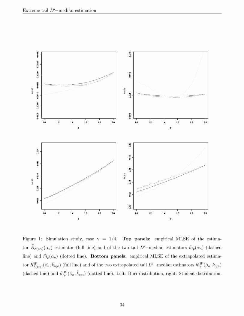
Extreme tail Lp−median estimation
1.0 1.2 1.4 1.6 1.8 2.0
0.0
00
00
.00
05
0.0
01
00
.00
15
0.0
02
00
.00
25
0.0
03
0
p
ML
SE
1.0 1.2 1.4 1.6 1.8 2.0
0.0
00
00
.00
05
0.0
01
00
.00
15
0.0
02
00
.00
25
0.0
03
0
p
1.0 1.2 1.4 1.6 1.8 2.0
0.0
00
00
.00
05
0.0
01
00
.00
15
0.0
02
00
.00
25
0.0
03
0
p
1.0 1.2 1.4 1.6 1.8 2.0
0.0
00
0.0
05
0.0
10
0.0
15
p
ML
SE
1.0 1.2 1.4 1.6 1.8 2.0
0.0
00
0.0
05
0.0
10
0.0
15
p
1.0 1.2 1.4 1.6 1.8 2.0
0.0
00
0.0
05
0.0
10
0.0
15
p
1.0 1.2 1.4 1.6 1.8 2.0
0.0
26
0.0
28
0.0
30
0.0
32
0.0
34
p
ML
SE
1.0 1.2 1.4 1.6 1.8 2.0
0.0
26
0.0
28
0.0
30
0.0
32
0.0
34
p
1.0 1.2 1.4 1.6 1.8 2.0
0.0
26
0.0
28
0.0
30
0.0
32
0.0
34
p
1.0 1.2 1.4 1.6 1.8 2.0
0.1
00
.12
0.1
40
.16
0.1
80
.20
p
ML
SE
1.0 1.2 1.4 1.6 1.8 2.0
0.1
00
.12
0.1
40
.16
0.1
80
.20
p
1.0 1.2 1.4 1.6 1.8 2.0
0.1
00
.12
0.1
40
.16
0.1
80
.20
p
Figure 1: Simulation study, case γ = 1/4. Top panels: empirical MLSE of the estima-
tor Rλ(p,γ)(αn) estimator (full line) and of the two tail Lp−median estimators mp(αn) (dashed
line) and mp(αn) (dotted line). Bottom panels: empirical MLSE of the extrapolated estima-
tor RWλ(p,γ)(βn, kopt) (full line) and of the two extrapolated tail Lp−median estimators mW
p (βn, kopt)
(dashed line) and mWp (βn, kopt) (dotted line). Left: Burr distribution, right: Student distribution.
34
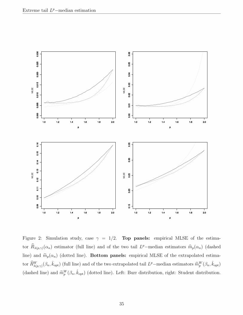
Extreme tail Lp−median estimation
1.0 1.2 1.4 1.6 1.8 2.0
0.0
00
0.0
05
0.0
10
0.0
15
0.0
20
0.0
25
0.0
30
p
ML
SE
1.0 1.2 1.4 1.6 1.8 2.0
0.0
00
0.0
05
0.0
10
0.0
15
0.0
20
0.0
25
0.0
30
p
1.0 1.2 1.4 1.6 1.8 2.0
0.0
00
0.0
05
0.0
10
0.0
15
0.0
20
0.0
25
0.0
30
p
1.0 1.2 1.4 1.6 1.8 2.0
0.0
00
.01
0.0
20
.03
0.0
40
.05
0.0
6p
ML
SE
1.0 1.2 1.4 1.6 1.8 2.0
0.0
00
.01
0.0
20
.03
0.0
40
.05
0.0
6p
1.0 1.2 1.4 1.6 1.8 2.0
0.0
00
.01
0.0
20
.03
0.0
40
.05
0.0
6p
1.0 1.2 1.4 1.6 1.8 2.0
0.0
90
.10
0.1
10
.12
0.1
30
.14
0.1
50
.16
p
ML
SE
1.0 1.2 1.4 1.6 1.8 2.0
0.0
90
.10
0.1
10
.12
0.1
30
.14
0.1
50
.16
p
1.0 1.2 1.4 1.6 1.8 2.0
0.0
90
.10
0.1
10
.12
0.1
30
.14
0.1
50
.16
p
1.0 1.2 1.4 1.6 1.8 2.0
0.1
50
.20
0.2
50
.30
0.3
5
p
ML
SE
1.0 1.2 1.4 1.6 1.8 2.0
0.1
50
.20
0.2
50
.30
0.3
5
p
1.0 1.2 1.4 1.6 1.8 2.0
0.1
50
.20
0.2
50
.30
0.3
5
p
Figure 2: Simulation study, case γ = 1/2. Top panels: empirical MLSE of the estima-
tor Rλ(p,γ)(αn) estimator (full line) and of the two tail Lp−median estimators mp(αn) (dashed
line) and mp(αn) (dotted line). Bottom panels: empirical MLSE of the extrapolated estima-
tor RWλ(p,γ)(βn, kopt) (full line) and of the two extrapolated tail Lp−median estimators mW
p (βn, kopt)
(dashed line) and mWp (βn, kopt) (dotted line). Left: Burr distribution, right: Student distribution.
35
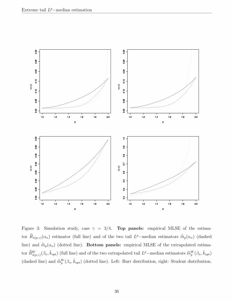
Extreme tail Lp−median estimation
1.0 1.2 1.4 1.6 1.8 2.0
0.0
00
.05
0.1
00
.15
0.2
00
.25
0.3
0
p
ML
SE
1.0 1.2 1.4 1.6 1.8 2.0
0.0
00
.05
0.1
00
.15
0.2
00
.25
0.3
0
p
1.0 1.2 1.4 1.6 1.8 2.0
0.0
00
.05
0.1
00
.15
0.2
00
.25
0.3
0
p
1.0 1.2 1.4 1.6 1.8 2.0
0.0
00
.05
0.1
00
.15
0.2
00
.25
0.3
0p
ML
SE
1.0 1.2 1.4 1.6 1.8 2.0
0.0
00
.05
0.1
00
.15
0.2
00
.25
0.3
0p
1.0 1.2 1.4 1.6 1.8 2.0
0.0
00
.05
0.1
00
.15
0.2
00
.25
0.3
0p
1.0 1.2 1.4 1.6 1.8 2.0
0.2
00
.25
0.3
00
.35
0.4
00
.45
0.5
00
.55
p
ML
SE
1.0 1.2 1.4 1.6 1.8 2.0
0.2
00
.25
0.3
00
.35
0.4
00
.45
0.5
00
.55
p
1.0 1.2 1.4 1.6 1.8 2.0
0.2
00
.25
0.3
00
.35
0.4
00
.45
0.5
00
.55
p
1.0 1.2 1.4 1.6 1.8 2.0
0.3
0.4
0.5
0.6
0.7
0.8
0.9
1.0
p
ML
SE
1.0 1.2 1.4 1.6 1.8 2.0
0.3
0.4
0.5
0.6
0.7
0.8
0.9
1.0
p
1.0 1.2 1.4 1.6 1.8 2.0
0.3
0.4
0.5
0.6
0.7
0.8
0.9
1.0
p
Figure 3: Simulation study, case γ = 3/4. Top panels: empirical MLSE of the estima-
tor Rλ(p,γ)(αn) estimator (full line) and of the two tail Lp−median estimators mp(αn) (dashed
line) and mp(αn) (dotted line). Bottom panels: empirical MLSE of the extrapolated estima-
tor RWλ(p,γ)(βn, kopt) (full line) and of the two extrapolated tail Lp−median estimators mW
p (βn, kopt)
(dashed line) and mWp (βn, kopt) (dotted line). Left: Burr distribution, right: Student distribution.
36
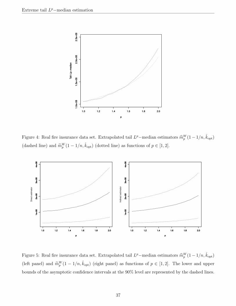
Extreme tail Lp−median estimation
1.0 1.2 1.4 1.6 1.8 2.0
1.0
e+
08
1.5
e+
08
2.0
e+
08
2.5
e+
08
p
Ta
il−L
p−
me
dia
n
1.0 1.2 1.4 1.6 1.8 2.0
1.0
e+
08
1.5
e+
08
2.0
e+
08
2.5
e+
08
p
Ta
il−L
p−
me
dia
n
Figure 4: Real fire insurance data set. Extrapolated tail Lp−median estimators mWp (1− 1/n, kopt)
(dashed line) and mWp (1− 1/n, kopt) (dotted line) as functions of p ∈ [1, 2].
1.0 1.2 1.4 1.6 1.8 2.0
1e
+0
82
e+
08
3e
+0
84
e+
08
p
Dire
ct
estim
ato
r
1.0 1.2 1.4 1.6 1.8 2.0
1e
+0
82
e+
08
3e
+0
84
e+
08
p
1.0 1.2 1.4 1.6 1.8 2.0
1e
+0
82
e+
08
3e
+0
84
e+
08
p
1.0 1.2 1.4 1.6 1.8 2.0
1e
+0
82
e+
08
3e
+0
84
e+
08
p
Ind
ire
ct
estim
ato
r
1.0 1.2 1.4 1.6 1.8 2.0
1e
+0
82
e+
08
3e
+0
84
e+
08
p
1.0 1.2 1.4 1.6 1.8 2.0
1e
+0
82
e+
08
3e
+0
84
e+
08
p
Figure 5: Real fire insurance data set. Extrapolated tail Lp−median estimators mWp (1− 1/n, kopt)
(left panel) and mWp (1 − 1/n, kopt) (right panel) as functions of p ∈ [1, 2]. The lower and upper
bounds of the asymptotic confidence intervals at the 90% level are represented by the dashed lines.
37