Graduate Theses and Dissertations Iowa State University Capstones, Theses andDissertations

2016

Exploring regularities in software with statisticalmodels and their applicationsAnh Tuan NguyenIowa State University

Follow this and additional works at: https://lib.dr.iastate.edu/etd

Part of the Computer Engineering Commons

This Dissertation is brought to you for free and open access by the Iowa State University Capstones, Theses and Dissertations at Iowa State UniversityDigital Repository. It has been accepted for inclusion in Graduate Theses and Dissertations by an authorized administrator of Iowa State UniversityDigital Repository. For more information, please contact digirep@iastate.edu.

Recommended CitationNguyen, Anh Tuan, "Exploring regularities in software with statistical models and their applications" (2016). Graduate Theses andDissertations. 15069.https://lib.dr.iastate.edu/etd/15069

Exploring regularities in software with statistical models and their applications

by

Anh Tuan Nguyen

A dissertation submitted to the graduate faculty

in partial ful�llment of the requirements for the degree of

DOCTOR OF PHILOSOPHY

Major: Computer Engineering

Program of Study Committee:

Tien N. Nguyen, Major Professor

Morris Chang

Manimaran Govindarasu

Jin Tian

Zhao Zhang

Iowa State University

Ames, Iowa

2016

Copyright c© Anh Tuan Nguyen, 2016. All rights reserved.

ii

TABLE OF CONTENTS

LIST OF TABLES . . . . . . . . . . . . . . . . . . . . . . . . . . . . . . . . . . . . vii

LIST OF FIGURES . . . . . . . . . . . . . . . . . . . . . . . . . . . . . . . . . . . x

ACKNOWLEDGEMENTS . . . . . . . . . . . . . . . . . . . . . . . . . . . . . . . xv

ABSTRACT . . . . . . . . . . . . . . . . . . . . . . . . . . . . . . . . . . . . . . . . xvi

CHAPTER 1. INTRODUCTION . . . . . . . . . . . . . . . . . . . . . . . . . . 1

1.1 Overview . . . . . . . . . . . . . . . . . . . . . . . . . . . . . . . . . . . . . . . 2

1.2 Related Publications and Works under Submission . . . . . . . . . . . . . . . . 4

1.2.1 Related Publications . . . . . . . . . . . . . . . . . . . . . . . . . . . . . 4

1.2.2 Works under Submission . . . . . . . . . . . . . . . . . . . . . . . . . . . 5

CHAPTER 2. ON THE EMPIRICAL STUDY ABOUT NATURALNESS/

REPETIVENESS OF SOURCE CODE AND CHANGES . . . . . . . . . . 6

2.1 A Large-Scale Study On Repetitiveness, Containment, and Composability of

Routines in Open-Source Projects . . . . . . . . . . . . . . . . . . . . . . . . . . 6

2.1.1 Data Collection and Concepts . . . . . . . . . . . . . . . . . . . . . . . . 7

2.1.2 Experimental Methodology . . . . . . . . . . . . . . . . . . . . . . . . . 13

2.1.3 Repeated Entire Routines . . . . . . . . . . . . . . . . . . . . . . . . . . 17

2.1.4 Containment among Routines . . . . . . . . . . . . . . . . . . . . . . . . 23

2.1.5 Composability of Routines . . . . . . . . . . . . . . . . . . . . . . . . . . 25

2.1.6 Repeated and Co-occuring Subroutines . . . . . . . . . . . . . . . . . . . 26

2.1.7 Repetitiveness of JDK API Usages . . . . . . . . . . . . . . . . . . . . . 29

2.2 Naturalness of Source Code Changes . . . . . . . . . . . . . . . . . . . . . . . . 31

2.2.1 Introduction . . . . . . . . . . . . . . . . . . . . . . . . . . . . . . . . . . 31

iii

2.2.2 Code Change Representation . . . . . . . . . . . . . . . . . . . . . . . . 32

2.2.3 Modeling Task Context with LDA . . . . . . . . . . . . . . . . . . . . . 39

2.2.4 Change Suggestion Algorithm . . . . . . . . . . . . . . . . . . . . . . . . 41

2.2.5 Empirical Evaluation . . . . . . . . . . . . . . . . . . . . . . . . . . . . . 43

2.3 Discussion . . . . . . . . . . . . . . . . . . . . . . . . . . . . . . . . . . . . . . . 56

CHAPTER 3. MODELS . . . . . . . . . . . . . . . . . . . . . . . . . . . . . . . . 58

3.1 Overview . . . . . . . . . . . . . . . . . . . . . . . . . . . . . . . . . . . . . . . 58

3.2 Background about Models in Natural Language Processing . . . . . . . . . . . . 59

3.2.1 Topic Model with LDA . . . . . . . . . . . . . . . . . . . . . . . . . . . 59

3.2.2 Language Models in Natural Language Processing . . . . . . . . . . . . 60

3.2.3 Statistical Translation Model in Natural Language Processing . . . . . . 63

3.3 Topic Models for Software . . . . . . . . . . . . . . . . . . . . . . . . . . . . . . 67

3.3.1 Topic Model for Source Code (S-Component) . . . . . . . . . . . . . . . 67

3.4 Deterministic Pattern-based Model . . . . . . . . . . . . . . . . . . . . . . . . . 70

3.4.1 Groum - Graph-based Representation of API Usage . . . . . . . . . . . 70

3.4.2 Deterministic Pattern-based Model with Groum . . . . . . . . . . . . . . 71

3.5 Deep Neural Network-based Models . . . . . . . . . . . . . . . . . . . . . . . . . 73

3.5.1 DNN Models for Language Models . . . . . . . . . . . . . . . . . . . . . 73

3.6 Graph-based Model . . . . . . . . . . . . . . . . . . . . . . . . . . . . . . . . . . 78

3.6.1 Bayesian-based Generation Model . . . . . . . . . . . . . . . . . . . . . 78

CHAPTER 4. APPLICATIONS: FINDING LINKING BETWEEN SOFT-

WARE ARTIFACTS . . . . . . . . . . . . . . . . . . . . . . . . . . . . . . . . . 82

4.1 Bug Localization . . . . . . . . . . . . . . . . . . . . . . . . . . . . . . . . . . . 82

4.1.1 Problem Statement . . . . . . . . . . . . . . . . . . . . . . . . . . . . . . 82

4.1.2 Approach using Topic Model . . . . . . . . . . . . . . . . . . . . . . . . 83

4.1.3 Evaluation . . . . . . . . . . . . . . . . . . . . . . . . . . . . . . . . . . . 89

4.2 Bug Duplication Detection . . . . . . . . . . . . . . . . . . . . . . . . . . . . . . 96

4.2.1 Problem Statement . . . . . . . . . . . . . . . . . . . . . . . . . . . . . . 96

iv

4.2.2 Approach using Combination of Topic Model and Information Retrieval 97

CHAPTER 5. APPLICATIONS: SOURCE CODE ANDAPI RECOMMEN-

DATION . . . . . . . . . . . . . . . . . . . . . . . . . . . . . . . . . . . . . . . . 113

5.1 DNN4C: Code Recommendation using Deep Neural Network-based model . . . 113

5.1.1 DNN Language Model for Code . . . . . . . . . . . . . . . . . . . . . . . 113

5.1.2 Empirical Evaluation . . . . . . . . . . . . . . . . . . . . . . . . . . . . . 118

5.1.3 Impacts of Factors on Accuracy . . . . . . . . . . . . . . . . . . . . . . . 120

5.1.4 Accuracy Comparison . . . . . . . . . . . . . . . . . . . . . . . . . . . . 123

5.1.5 Time E�ciency . . . . . . . . . . . . . . . . . . . . . . . . . . . . . . . . 127

5.1.6 Case Studies . . . . . . . . . . . . . . . . . . . . . . . . . . . . . . . . . 128

5.1.7 Examples on Neighboring Sequences . . . . . . . . . . . . . . . . . . . . 129

5.1.8 Limitations and Threats to Validity . . . . . . . . . . . . . . . . . . . . 130

5.2 GraPacc: API Usage Recommendation using Pattern-based Model . . . . . . . 131

5.2.1 Important Concepts . . . . . . . . . . . . . . . . . . . . . . . . . . . . . 131

5.2.2 Query Processing and Feature Extraction . . . . . . . . . . . . . . . . . 132

5.2.3 Pattern Managing, Searching and Ranking . . . . . . . . . . . . . . . . . 136

5.2.4 Pattern-Oriented Code Completion . . . . . . . . . . . . . . . . . . . . . 139

5.2.5 Matching Groum Nodes in Pattern and Query . . . . . . . . . . . . . . . 140

5.2.6 Completing the Query Code . . . . . . . . . . . . . . . . . . . . . . . . . 141

5.2.7 Empirical Evaluation . . . . . . . . . . . . . . . . . . . . . . . . . . . . . 142

5.3 GraLan: API Usage Recommendation using Graph-based Model . . . . . . . . 149

5.3.1 Computation based on Bayesian Statistical Inference . . . . . . . . . . . 149

5.3.2 GraLan in API Element Suggestion . . . . . . . . . . . . . . . . . . . . . 151

5.3.3 AST-based Language Model . . . . . . . . . . . . . . . . . . . . . . . . . 155

5.3.4 Empirical Evaluation . . . . . . . . . . . . . . . . . . . . . . . . . . . . . 160

CHAPTER 6. APPLICATIONS: MAPPING AND TRANSLATION . . . . . 169

6.1 JV2CS: Statistical Learning of API Mappings for Code Migration with Vector

Transformations . . . . . . . . . . . . . . . . . . . . . . . . . . . . . . . . . . . . 169

v

6.1.1 Research Problem . . . . . . . . . . . . . . . . . . . . . . . . . . . . . . 169

6.1.2 Approach Overview . . . . . . . . . . . . . . . . . . . . . . . . . . . . . 170

6.1.3 Illustrating Example . . . . . . . . . . . . . . . . . . . . . . . . . . . . . 172

6.1.4 Vector Representation . . . . . . . . . . . . . . . . . . . . . . . . . . . . 174

6.1.5 Building API Sequences . . . . . . . . . . . . . . . . . . . . . . . . . . . 176

6.1.6 Transformation between Two Vector Spaces in Java and C# . . . . . . . 179

6.1.7 Empirical Evaluation . . . . . . . . . . . . . . . . . . . . . . . . . . . . . 181

6.1.8 Conclusion . . . . . . . . . . . . . . . . . . . . . . . . . . . . . . . . . . 195

6.2 mppSMT: Cross Language Source Code Translation . . . . . . . . . . . . . . . 196

6.2.1 Mapping of Sequences of Syntactic Units . . . . . . . . . . . . . . . . . . 196

6.2.2 Mappings of Token Types and Data Types . . . . . . . . . . . . . . . . . 199

6.2.3 Training and Translation . . . . . . . . . . . . . . . . . . . . . . . . . . . 201

6.2.4 Multi-phase Translation Algorithm . . . . . . . . . . . . . . . . . . . . . 204

6.2.5 Empirical Evaluation . . . . . . . . . . . . . . . . . . . . . . . . . . . . . 206

6.3 T2API: Text to Code Translation . . . . . . . . . . . . . . . . . . . . . . . . . . 215

6.3.1 Approach Overview . . . . . . . . . . . . . . . . . . . . . . . . . . . . . 215

6.3.2 Mapping & API Element Inferring . . . . . . . . . . . . . . . . . . . . . 222

6.3.3 Infer API Elements for a Given Query . . . . . . . . . . . . . . . . . . . 224

6.3.4 Synthesizing API Usages . . . . . . . . . . . . . . . . . . . . . . . . . . . 225

6.3.5 Empirical Evaluation . . . . . . . . . . . . . . . . . . . . . . . . . . . . . 230

6.3.6 Limitations . . . . . . . . . . . . . . . . . . . . . . . . . . . . . . . . . . 237

CHAPTER 7. RELATED WORK . . . . . . . . . . . . . . . . . . . . . . . . . . 240

7.1 Empirical Study on Naturalness and Repetitiveness . . . . . . . . . . . . . . . . 240

7.2 Language Models . . . . . . . . . . . . . . . . . . . . . . . . . . . . . . . . . . . 241

7.3 Code Recommendation . . . . . . . . . . . . . . . . . . . . . . . . . . . . . . . . 242

7.4 Code to Code Translation . . . . . . . . . . . . . . . . . . . . . . . . . . . . . . 244

7.5 Text to Code Translation . . . . . . . . . . . . . . . . . . . . . . . . . . . . . . 246

vi

CHAPTER 8. FUTURE WORK AND CONCLUSIONS . . . . . . . . . . . . 249

8.1 Future Work . . . . . . . . . . . . . . . . . . . . . . . . . . . . . . . . . . . . . 249

8.1.1 Empirical . . . . . . . . . . . . . . . . . . . . . . . . . . . . . . . . . . . 249

8.1.2 Models . . . . . . . . . . . . . . . . . . . . . . . . . . . . . . . . . . . . . 250

8.1.3 Applications . . . . . . . . . . . . . . . . . . . . . . . . . . . . . . . . . . 253

8.2 Conclusions . . . . . . . . . . . . . . . . . . . . . . . . . . . . . . . . . . . . . . 255

BIBLIOGRAPHY . . . . . . . . . . . . . . . . . . . . . . . . . . . . . . . . . . . . 256

vii

LIST OF TABLES

Table 2.1 Collected Dataset . . . . . . . . . . . . . . . . . . . . . . . . . . . . . . 7

Table 2.2 Graph operators and functions in gOOQ . . . . . . . . . . . . . . . . . 13

Table 2.3 Example of n-path features and indexes . . . . . . . . . . . . . . . . . . 14

Table 2.4 Repetitiveness without and without control nodes . . . . . . . . . . . . 21

Table 2.5 Repetitiveness by number of nested control structures . . . . . . . . . . 22

Table 2.6 Frequent (Sub)routines and Co-occurring Routines . . . . . . . . . . . 31

Table 2.7 Statistics on frequencies of JDK API usages . . . . . . . . . . . . . . . 32

Table 2.8 Collected Projects and Code Changes . . . . . . . . . . . . . . . . . . . 44

Table 2.9 Suggestion accuracy comparison between the model using task context

and base models. . . . . . . . . . . . . . . . . . . . . . . . . . . . . . . 49

Table 2.10 Change suggestion accuracy comparison between using task context and

using other contexts . . . . . . . . . . . . . . . . . . . . . . . . . . . . . 54

Table 2.11 Accuracy comparison between contexts . . . . . . . . . . . . . . . . . . 55

Table 2.12 Empirical Studies in Naturalness of Software . . . . . . . . . . . . . . . 57

Table 4.1 Subject Systems . . . . . . . . . . . . . . . . . . . . . . . . . . . . . . . 91

Table 4.2 Time E�ciency . . . . . . . . . . . . . . . . . . . . . . . . . . . . . . . 96

Table 4.3 Statistics of All Bug Report Data . . . . . . . . . . . . . . . . . . . . . 106

Table 5.1 Subject Projects . . . . . . . . . . . . . . . . . . . . . . . . . . . . . . . 119

Table 5.2 Accuracy With Di�erent Sizes of Contexts . . . . . . . . . . . . . . . . 121

Table 5.3 Accuracy With Di�erent Contexts . . . . . . . . . . . . . . . . . . . . . 122

Table 5.4 Accuracy Comparison on All Projects . . . . . . . . . . . . . . . . . . . 124

Table 5.5 Mean Reciprocal Rank (MRR) Comparison . . . . . . . . . . . . . . . 125

viii

Table 5.6 Comparison of Dnn4C and Bayesian-based LM . . . . . . . . . . . . . . 127

Table 5.7 Training Time (in hours) . . . . . . . . . . . . . . . . . . . . . . . . . . 128

Table 5.8 Examples of Nearest Neighbors of Sequences in Db4o . . . . . . . . . . 130

Table 5.9 Training data for Java Utility Patterns . . . . . . . . . . . . . . . . . . 143

Table 5.10 Code Completion Accuracy Result . . . . . . . . . . . . . . . . . . . . . 146

Table 5.11 Context Graphs and Their Children Graphs . . . . . . . . . . . . . . . 154

Table 5.12 Ranked Candidate Nodes . . . . . . . . . . . . . . . . . . . . . . . . . . 154

Table 5.13 Examples of Expanding Rules . . . . . . . . . . . . . . . . . . . . . . . 158

Table 5.14 Data Collection . . . . . . . . . . . . . . . . . . . . . . . . . . . . . . . 161

Table 5.15 Accuracy % with Di�erent Numbers of Closest Nodes . . . . . . . . . . 162

Table 5.16 Accuracy % with Di�erent Maximum Context Graphs' Sizes . . . . . . 162

Table 5.17 Accuracy % with Di�erent Datasets . . . . . . . . . . . . . . . . . . . . 163

Table 5.18 API Suggestion Accuracy Comparison . . . . . . . . . . . . . . . . . . 164

Table 5.19 Accuracy % with Di�erent Maximum Heights of Context Trees . . . . . 165

Table 5.20 Accuracy % of ASTLan with Di�erent Datasets . . . . . . . . . . . . . 166

Table 5.21 Statistics on Graph Database . . . . . . . . . . . . . . . . . . . . . . . 167

Table 5.22 Statistics on Tree Database . . . . . . . . . . . . . . . . . . . . . . . . 167

Table 6.1 Key Rules S(E) to Build API Sequences in Java . . . . . . . . . . . . 178

Table 6.2 Datasets to build Word2Vec vectors . . . . . . . . . . . . . . . . . . . . 182

Table 6.3 Examples of APIs sharing similar surrounding APIs . . . . . . . . . . . 183

Table 6.4 t-test results for vector distances of APIs in the same and di�ferent

classes and packages . . . . . . . . . . . . . . . . . . . . . . . . . . . . 185

Table 6.5 Example Relations via Vector O�sets in JDK . . . . . . . . . . . . . . 186

Table 6.6 Some newly found API mappings that were not in Java2CSharp's man-

ually written mapping data �les . . . . . . . . . . . . . . . . . . . . . . 193

Table 6.7 Migration of API usage sequences . . . . . . . . . . . . . . . . . . . . . 194

Table 6.8 Examples of Java syntax and function encode to produce a sequence of

syntaxemes for Java code . . . . . . . . . . . . . . . . . . . . . . . . . . 196

ix

Table 6.9 Examples of C# syntax and function encode to produce a sequence of

syntaxemes for C# code . . . . . . . . . . . . . . . . . . . . . . . . . . . 197

Table 6.10 Examples of Sememes [174] . . . . . . . . . . . . . . . . . . . . . . . . 200

Table 6.11 Subject Systems . . . . . . . . . . . . . . . . . . . . . . . . . . . . . . . 202

Table 6.12 Accuracy Comparison (max/min values highlighted) . . . . . . . . . . . 207

Table 6.13 %Results Exact-matched to Human-Written C# . . . . . . . . . . . . . 208

Table 6.14 API Mappings and Other Migration Rules . . . . . . . . . . . . . . . . 209

Table 6.15 Accuracy with Cross-Project Training . . . . . . . . . . . . . . . . . . . 210

Table 6.16 Training Time (in minutes per project) . . . . . . . . . . . . . . . . . . 210

Table 6.17 Translation Time (in seconds per method) . . . . . . . . . . . . . . . . 211

Table 6.18 ZXing and ZXing.Net . . . . . . . . . . . . . . . . . . . . . . . . . . . . 211

Table 6.19 Accuracy with Updated Phrase Translation Table . . . . . . . . . . . . 212

Table 6.20 StackOver�ow Dataset for Training Mapping Model . . . . . . . . . . . 230

Table 6.21 Accuracy in Code Element Inferring with/wo Pivots . . . . . . . . . . . 232

Table 6.22 Statistics of Dataset for Training the Graph Synthesizing (Language)

Model . . . . . . . . . . . . . . . . . . . . . . . . . . . . . . . . . . . . 233

Table 6.23 Accumulative Accuracy . . . . . . . . . . . . . . . . . . . . . . . . . . . 234

Table 6.24 Graph Synthesizing Accuracy . . . . . . . . . . . . . . . . . . . . . . . 234

Table 6.25 Precision and Recall Distributions for Nodes and Edges over 250 Testing

Posts . . . . . . . . . . . . . . . . . . . . . . . . . . . . . . . . . . . . . 235

Table 6.26 Time and Space Complexity . . . . . . . . . . . . . . . . . . . . . . . . 238

x

LIST OF FIGURES

Figure 1.1 Overview . . . . . . . . . . . . . . . . . . . . . . . . . . . . . . . . . . . 3

Figure 2.1 Example of a routine . . . . . . . . . . . . . . . . . . . . . . . . . . . . 8

Figure 2.2 Program Dependence Graph (PDG) for code in Figure 2.1 . . . . . . . 8

Figure 2.3 Enhancing PDG with API nodes and dependency edges . . . . . . . . . 10

Figure 2.4 Per-variable slicing subgraphs in PDG . . . . . . . . . . . . . . . . . . 12

Figure 2.5 Example of gOOQ query . . . . . . . . . . . . . . . . . . . . . . . . . . 13

Figure 2.6 % of entire routines realized elsewhere within a project . . . . . . . . . 17

Figure 2.7 % of entire routines realized in more than one project . . . . . . . . . . 18

Figure 2.8 % of entire routines realized elsewhere in other projects . . . . . . . . . 19

Figure 2.9 Repetitiveness by graph size (|V |+ |E|) in PDG . . . . . . . . . . . . . 20

Figure 2.10 Repetitiveness by cyclomatic complexity . . . . . . . . . . . . . . . . . 21

Figure 2.11 Repetitiveness by number of control nodes in PDG . . . . . . . . . . . 22

Figure 2.12 % of routines realized as part of other routine(s) elsewhere within a

project. Horizontal axis shows number of containers. . . . . . . . . . . 23

Figure 2.13 % of routines realized as part of other routine(s) elsewhere in other

projects. Horizontal axis shows number of containers. . . . . . . . . . . 24

Figure 2.14 Containment by graph size (|E| + |V |) in PDG . . . . . . . . . . . . . 25

Figure 2.15 Containment by cyclomatic complexity . . . . . . . . . . . . . . . . . . 26

Figure 2.16 Cumulative distribution of routines with respect to percentage of their

repeated subroutines . . . . . . . . . . . . . . . . . . . . . . . . . . . . 27

Figure 2.17 Repetitiveness of subroutines by size (|V |+ |E|) . . . . . . . . . . . . . 28

Figure 2.18 Repetitiveness of JDK subroutines by size (|V |+ |E|) . . . . . . . . . . 29

xi

Figure 2.19 Cumulative distribution of pairs of subroutines w.r.t. their Jaccard indexes 30

Figure 2.20 Most and least frequently used JDK APIs . . . . . . . . . . . . . . . . 32

Figure 2.21 Percentage of JDK usages repeated at various average numbers from

1�10 (per project) of their frequent occurrences . . . . . . . . . . . . . 33

Figure 2.22 Usage comparison in JDK packages. The Y-axis shows the numbers of

distinct usages occurring with speci�c frequencies. . . . . . . . . . . . . 34

Figure 2.23 An Example of Code Change . . . . . . . . . . . . . . . . . . . . . . . . 34

Figure 2.24 Tree-based Representation for the Code Change in Figure 2.23 . . . . . 35

Figure 2.25 Extracted Code Changes for the Example in Figure 2.24 . . . . . . . . 37

Figure 2.26 LDA-based Task Context Modeling . . . . . . . . . . . . . . . . . . . . 40

Figure 2.27 Change Suggestion Algorithm . . . . . . . . . . . . . . . . . . . . . . . 43

Figure 2.28 Sensitivity analysis on the impact of the similarity threshold to the sug-

gestion accuracy in project ONDEX. . . . . . . . . . . . . . . . . . . . 46

Figure 2.29 Sensitivity analysis on the impact of the number of tasks/topics to the

suggestion accuracy in project ONDEX. . . . . . . . . . . . . . . . . . 47

Figure 2.30 Temporal locality of task context. . . . . . . . . . . . . . . . . . . . . . 47

Figure 2.31 Spatial locality of task context. . . . . . . . . . . . . . . . . . . . . . . 48

Figure 2.32 Suggestion accuracy comparison between �xing and general changes us-

ing task context. . . . . . . . . . . . . . . . . . . . . . . . . . . . . . . . 51

Figure 2.33 Top-1 suggestion accuracy comparison between using task context and

using other contexts. . . . . . . . . . . . . . . . . . . . . . . . . . . . . 53

Figure 2.34 Case Studies . . . . . . . . . . . . . . . . . . . . . . . . . . . . . . . . . 56

Figure 2.35 Case Studies . . . . . . . . . . . . . . . . . . . . . . . . . . . . . . . . . 56

Figure 3.1 Models Used in NLP and Corresponding Models in Source Code Processing 58

Figure 3.2 Topic Model . . . . . . . . . . . . . . . . . . . . . . . . . . . . . . . . . 59

Figure 3.3 Statistical Machine Translation (SMT) . . . . . . . . . . . . . . . . . . 63

Figure 3.4 Example of phrase-based translation [113] . . . . . . . . . . . . . . . . 66

Figure 3.5 Parent and Children Graphs . . . . . . . . . . . . . . . . . . . . . . . . 70

xii

Figure 3.6 SWT Usage Example 1 . . . . . . . . . . . . . . . . . . . . . . . . . . . 71

Figure 3.7 SWT Usage Patterns . . . . . . . . . . . . . . . . . . . . . . . . . . . . 72

Figure 3.8 Context-aware DNN-based Model: Incorporating Syntactic and Seman-

tic Contexts . . . . . . . . . . . . . . . . . . . . . . . . . . . . . . . . . 73

Figure 3.9 Dnn4C: Deep Neural Network Language Model for Code . . . . . . . . 76

Figure 3.10 Parent and Children Graphs . . . . . . . . . . . . . . . . . . . . . . . . 80

Figure 4.1 BugScout Model . . . . . . . . . . . . . . . . . . . . . . . . . . . . . . . 83

Figure 4.2 Model Training Algorithm . . . . . . . . . . . . . . . . . . . . . . . . . 86

Figure 4.3 Predicting and Recommending Algorithm . . . . . . . . . . . . . . . . 89

Figure 4.4 Accuracy and the Number of Topics without P(s) . . . . . . . . . . . . 92

Figure 4.5 Accuracy and the Number of Topics with P(s) . . . . . . . . . . . . . . 93

Figure 4.6 Accuracy Comparison on Jazz dataset . . . . . . . . . . . . . . . . . . 94

Figure 4.7 Accuracy Comparison on AspectJ dataset . . . . . . . . . . . . . . . . 95

Figure 4.8 Accuracy Comparison on Eclipse dataset . . . . . . . . . . . . . . . . . 95

Figure 4.9 Accuracy Comparison on ArgoUML dataset . . . . . . . . . . . . . . . 96

Figure 4.10 Topic Model for Bug Reports . . . . . . . . . . . . . . . . . . . . . . . 97

Figure 4.11 Bug Report BR2 in Eclipse Project . . . . . . . . . . . . . . . . . . . . 98

Figure 4.12 Bug Report BR9779, a Duplicate of BR2 . . . . . . . . . . . . . . . . . 98

Figure 4.13 Prediction Algorithm . . . . . . . . . . . . . . . . . . . . . . . . . . . . 103

Figure 4.14 Ensemble Weight Training Algorithm . . . . . . . . . . . . . . . . . . . 105

Figure 4.15 Accuracy with Varied Numbers of Topics . . . . . . . . . . . . . . . . . 107

Figure 4.16 Accuracy Comparison in Eclipse . . . . . . . . . . . . . . . . . . . . . . 108

Figure 4.17 Accuracy Comparison in OpenO�ce . . . . . . . . . . . . . . . . . . . 109

Figure 4.18 Accuracy Comparison in Mozilla . . . . . . . . . . . . . . . . . . . . . . 110

Figure 4.19 Time E�ciency . . . . . . . . . . . . . . . . . . . . . . . . . . . . . . . 110

Figure 4.20 Duplicate Bug Reports in Eclipse . . . . . . . . . . . . . . . . . . . . . 112

Figure 5.1 Context-aware DNN-based Model: Incorporating Syntactic and Seman-

tic Contexts . . . . . . . . . . . . . . . . . . . . . . . . . . . . . . . . . 114

xiii

Figure 5.2 Dnn4C: Deep Neural Network Language Model for Code . . . . . . . . 115

Figure 5.3 Top-k Accuracy with Varied Numbers of Hidden Nodes . . . . . . . . . 120

Figure 5.4 Top-k Accuracy of Di�erent Approaches on Db4o . . . . . . . . . . . . 125

Figure 5.5 SWT Query Example . . . . . . . . . . . . . . . . . . . . . . . . . . . . 131

Figure 5.6 SWT Usage Patterns . . . . . . . . . . . . . . . . . . . . . . . . . . . . 132

Figure 5.7 Graph-based Usage Model of Query . . . . . . . . . . . . . . . . . . . . 133

Figure 5.8 Groum Node Matching between Pattern P and Query Q . . . . . . . . 140

Figure 5.9 Code Completion from Pattern P to Query Q . . . . . . . . . . . . . . 141

Figure 5.10 An Example of a Test Method . . . . . . . . . . . . . . . . . . . . . . . 143

Figure 5.11 An API Suggestion Example and API Usage Graph . . . . . . . . . . . 151

Figure 5.12 API Suggestion Algorithm . . . . . . . . . . . . . . . . . . . . . . . . . 152

Figure 5.13 Context Subgraphs . . . . . . . . . . . . . . . . . . . . . . . . . . . . . 153

Figure 5.14 An Example of Suggesting a Valid Syntactic Template . . . . . . . . . 157

Figure 6.1 API Mappings between Java and C# [164] . . . . . . . . . . . . . . . . 173

Figure 6.2 Vector Representations for APIs in jv2cs with CBOW . . . . . . . . . . 174

Figure 6.3 Distributed vector representations for some APIs in Java (left) the cor-

responding APIs in C# (right) . . . . . . . . . . . . . . . . . . . . . . . 179

Figure 6.4 Training for Transformation Model . . . . . . . . . . . . . . . . . . . . 179

Figure 6.5 Distances among JDK API vectors within and cross classes . . . . . . . 185

Figure 6.6 Top-k accuracy with di�erent numbers of dimensions . . . . . . . . . . 188

Figure 6.7 Top-k accuracy with varied training datasets for Word2Vec . . . . . . . 189

Figure 6.8 Top-k accuracy with various numbers of training mappings . . . . . . . 190

Figure 6.9 Top-k accuracy with di�erent training data selections . . . . . . . . . . 190

Figure 6.10 Top-k accuracy comparison with IBM Model . . . . . . . . . . . . . . . 191

Figure 6.11 Alignments of Syntactic Symbols are Learned from Corpus . . . . . . . 198

Figure 6.12 Placeholder for an Anonymous Class . . . . . . . . . . . . . . . . . . . 199

Figure 6.13 Training Algorithms . . . . . . . . . . . . . . . . . . . . . . . . . . . . . 203

Figure 6.14 Translation Algorithms . . . . . . . . . . . . . . . . . . . . . . . . . . . 204

xiv

Figure 6.15 T2API as Statistical Machine Translation . . . . . . . . . . . . . . . . 215

Figure 6.16 StackOver�ow Question 9292954 . . . . . . . . . . . . . . . . . . . . . . 216

Figure 6.17 StackOver�ow Answer 9292954 . . . . . . . . . . . . . . . . . . . . . . 216

Figure 6.18 Training and API Element Inferring Examples . . . . . . . . . . . . . . 217

Figure 6.19 Graph-based API Usage Representation . . . . . . . . . . . . . . . . . 219

Figure 6.20 Graph Expansion via Graph-based Language Model . . . . . . . . . . . 220

Figure 6.21 API Element Inference Algorithm . . . . . . . . . . . . . . . . . . . . . 223

Figure 6.22 Graph Synthesizing Example for a Candidate Usage Graph . . . . . . . 227

Figure 6.23 Graph Synthesizing Algorithm . . . . . . . . . . . . . . . . . . . . . . . 228

xv

ACKNOWLEDGEMENTS

I would like to express my thanks to those who helped me on my way �nishing my PhD,

conducting research and writing this thesis.

My PhD work would not �nish without the advising of Dr. Tien Nguyen. He helped

me understand the important topics in software engineering, �nd good problems that can make

contribution to research and �x my mistakes. I would also like to thank my committee members

for their guide and e�ort of sharing ideas.

My work would not become successful without collaboration of my colleagues, especially

Dr. Hoan Nguyen, Dr. Tung Nguyen and Hung Nguyen. They did not only support my

work, contribute their thoughts, but also share their knowledge to develop my skills and my

understanding about SE.

Last but foremost, I would like to thanks my parents and other family's members. My

parents were the �rst to encourage me to follow my PhD degree at Iowa State University. Only

with them, I could �nd the best motivation to follow my research career, to overcome many

barriers that I met. My father, who denied his PhD work to take care of his family, always

want me to �nish the degree that he could not. My father passed away and could not wait until

these days to see I completing his desire. However, the way of his thinking, his excitement in

�nishing his jobs, his love to contribute to the development of society is the model that I want

to follow. I feel proud that I can partly learn his characteristics and use them to deal with a

long, hard PhD student career. My mother, who spend all of her love to my family and me,

xvi

ABSTRACT

Software systems are becoming popular. They are used with di�erent platforms for di�erent

applications. Software systems are developed with support from programming languages, which

help developers work conveniently. Programming languages can have di�erent paradigms with

di�erent form, syntactic structures, keywords, representation ways. In many cases, however,

programming languages are similar in di�erent important aspects: 1. They are used to support

description of speci�c tasks, 2. Source codes are written in languages and includes a limit set of

distinctive tokens, many tokens are repeated like keywords, function calls, and 3. They follow

speci�c syntactic rules to make machine understanding. Those points also re�ect the similarity

between programming language and natural language.

Due to its critical role in many applications, natural language processing (NLP) has been

studied much and given many promising results like automatic cross-language translation,

speech-to-text, information searching, etc. It is interesting to observe if there are similar charac-

teristics between natural language and programming language and whether techniques in NLP

can be reused for programming language processing? Recent works in software engineering (SE)

shows that their similarities between NLP and programming language processing and techniques

in NLP can be reused for PLP.

This dissertation introduces my works with contributions in study of characteristics of pro-

gramming languages, the models which employed them and the main applications that show

the usefulness of the proposed models. Study in both three aspects has draw interests from

software engineering community and received awards due to their innovation and applicability

I hope that this dissertation will bring a systematic view of how advantage techniques in

natural language processing and machine learning can be re-used and give huge bene�t for

programming language processing, and how those techniques are adapted with characteristics

of programming language and software systems.

1

CHAPTER 1. INTRODUCTION

Nowadays, software plays a more and more important role in human life. Many devices from

computer to wearable ones requires software. Software also plays important roles in scienti�c

and research activities. They are required for weather prediction, data collection and analysis,

etc. Government and society also need support from software, from power management, tra�c

management to voting activities.

The more the necessity of software, the more requirement of their development, mainte-

nance and management. Software now can appear in very large scale, with contribution of

many developer, many resources and if not managed well, they can be hard for development

and maintenance and cause catastrophic results. Those new dimensions require software engi-

neering systematically developing new methods/techniques/models/applications to make soft-

ware development/maintenance progress faster and more reliable. The new subjects of software

engineering (SE) studies are not limited in toy/simple software projects but very large/complex

ones in between a complex system of other artifacts. Older methods, which are limited by per-

formance or are not robust with large scale data, can not be reused. New classes of approaches

should be invented in this case.

One feasible way of extending new approaches is considering similar application in relevant

areas, which employ the e�cient models with large scale data like big data mining (Big DM),

machine learning (ML) and natural language processing (NLP). Many recent works in SE fo-

cus on the similarities between programming language in software and natural language for

documents, and how to employ those similarities.

Software are written in programming language. There exists di�erent languages with di�er-

ent paradigms. One common class of language is imperative languages with very high popularity

like C, Java, C#, etc. Software codes written by those languages are composed of keywords, code

2

elements and conform speci�c syntax rules and hierarchical rules (packages, classes, methods,

statements, etc.). Elements are constructed in speci�c orders to perform speci�c tasks.

Those properties suggest the similarity between software codes and natural language doc-

uments. A natural language document also follows speci�c syntax rules and hierarchical rules

(corpus, documents, paragraphs, sentences, etc.) and contains words. The similarities between

software and natural language documents about structure can lead to similarity about usage of

element in them.

Recent works in software engineering [82] reveals the similarity at token level between code

and document. It can be seen via the similarity about repetitiveness and regularity (with

entropy measurement) of tokens. My group at ISU also �nd it interesting and studied the

similarities at other di�erent levels like API usages and methods.

Those empirical studies are important at they suggest that, the techniques, which success-

fully employ characteristics in natural documents, can be employed correspondingly in software

code. Works by other groups and my ones prove the usefulness of techniques like n-gram,

Bayesian models, neural network in software code processing.

Based on those models, I and my collaborators have developed di�erent software engineering

applications. Those applications are used successfully with di�erent tasks like code recommen-

dation, code translation and text-to-code translation.

1.1 Overview

Figure 1.1 outlines the works relating to or studied by me and collaborators at Iowa State

University. Works with my major contribution are in white background. Related work are

shaded.

This thesis will be organized into three main parts:

• Empirical study. Regularity and repetitiveness of source code at di�erent levels are

studied . Some levels like code token are studied by other authors (see section 7.1). Some

other levels were studied by me and collaborators, and will be introduced in sections

2.1 and 2.2. The empirical studies are very important because they will lay the funda-

3

Naturalness/Repetitiveness

of routines

Empirical Study Model Application

Naturalness/Repetitiveness

of code changesDeterministic pattern-based model for API usages

Topic model for bug report

Deep neural network-based model for source

code

Asscociation-based model for code changes

Graph-based model for source code

Naturalness/Repetitiveness

of code tokens

Naturalness/Repetitiveness

of NLP words

Topic model for source code

Bug duplication detection

Bug localization

Code recommendation

API usage recommendation

Code change recommendation

N-gram model for source code

Mapping model across languages (IBM Model)

Source code translation accross

programming languages

Text-to-code translation

Figure 1.1 Overview

mental knowledge for constructing models. Moreover, it will help researcher understand

more clearly about link between natural language processing and programming language

processing.

• Models. In this part, I will introduce proposed models which employ knowledge learned

from empirical study and support di�erent tasks in software engineering. Introduced

models include topic model (section 3.3, pattern-based model (section 3.4), deep learning-

based model (section 3.5), and graph-based model (section 3.6) Many of those models

are derived from corresponding models in Natural Language Processing (NLP). However,

there are many aspects that we need to consider for those reuses. I will discuss about

those issues in each section.

• Important applications in software engineering that directly use proposed models. My

group has used models in di�erent applications like code recommendation, API mapping,

code translation, bug localization, etc. and evaluated them. The empirical evaluation

shows promising results and shows that the use of proposed models from NLP can be a

4

good direction in software engineering. I will present those applications in sections 4.1,

4.2, 5.1, 5.2, 5.3, 6.1, 6.2 and 6.3

1.2 Related Publications and Works under Submission

1.2.1 Related Publications

1. Nguyen, A.T., Nguyen, H.A., and Nguyen, T.N. A Large-Scale Study On Repetitive-

ness, Containment, and Composability of Routines in Open-Source Projects. The 13th

International Conference on Mining Software Repositories, MSR 2016 - To appear.

2. Nguyen, A.T, Nguyen, T.T, Nguyen, T.N. Divide-and-Conquer Approach for Multi-phase

Statistical Migration for Source Code. The 30th IEEE/ACM International Conference on

Automated Software Engineering , ASE 2015.

3. Nguyen, A.T., Nguyen, T.N. Graph-based Statistical Language Model for Code. The

37th International Conference on Software Engineering, ICSE 2015.

4. Nguyen, A.T., Nguyen, H.A., Nguyen, T.T., Nguyen, T.N. Statistical Learning Approach

for Mining API Usage Mappings for Code Migration. The 29th IEEE/ACM International

Conference on Automated Software Engineering , ASE 2014.

Best Paper/ACM SIGSOFT Distinguished Paper Award.

5. Nguyen, T.T., Nguyen, A.T., Nguyen, A.H., Nguyen, T.N. A Statistical Semantic Lan-

guage Model for Source Code. The 9th joint meeting of the European Software Engineering

Conference and the ACM SIGSOFT Symposium on the Foundations of Software Engineer-

ing, ESEC/FSE 2013.

6. Nguyen, H.A., Nguyen, A.T., Nguyen, T.T., Nguyen, T.N. A Study of Repetitiveness of

Code Changes in Software Evolution. The 28th IEEE/ACM International Conference on

Automated Software Engineering , ASE 2013.

Nominated for ACM SIGSOFT Distinguished Paper Award.

5

7. Nguyen, A.T., Nguyen, T.T., Nguyen, H.A., Tamrawi, A., Nguyen, H.V., Al-Kofahi,

J., and Nguyen, T.N. Graph-based Pattern-oriented, Context-sensitive Code Completion.

The 34th International Conference on Software Engineering, ICSE 2012.

8. Nguyen, A.T., Nguyen, T.T., Nguyen, A.H., and Nguyen, T.N. Multi-layered Approach

for Recovering Links between Bug Reports and Fixes. The 20th ACM SIGSOFT Inter-

national Symposium on the Foundations of Software Engineering, FSE 2012.

9. Nguyen, A.T., Nguyen, T.T., Nguyen, T.N, Lo, D., and Sun, C. Duplicate Bug Report

Detection with a Combination of Information Retrieval and Topic Modeling. The 27th

IEEE/ACM International Conference on Automated Software Engineering , ASE 2012.

ACM SIGSOFT Distinguished Paper Award.

10. Nguyen, A.T., Nguyen, T.T., Al-Kofahi, J., Nguyen, H.V., and Nguyen, T.N. A Topic-

based Approach for Narrowing the Search Space of Buggy Files from a Bug Report.

The 26th IEEE/ACM International Conference on Automated Software Engineering, ASE

2011.

Nominated for ACM SIGSOFT Distinguished Paper Award.

1.2.2 Works under Submission

1. Nguyen, A.T., Nguyen, T.D., and Nguyen, T.N. A Deep Neural Network Language Model

with Syntactic and Semantic Contexts for Java Source Code.

2. Nguyen, A.T., Rigby, P., Nguyen, T., Karan�l, M., and Nguyen, T.N. Statistical Trans-

lation of English Texts to API Code Usage Templates.

3. Nguyen, T.V., Nguyen, A.T., Phan, H.D., and Nguyen, T.N. Statistical Learning of API

Mappings for Code Migration with Vector Transformations

6

CHAPTER 2. ON THE EMPIRICAL STUDY ABOUT NATURALNESS/

REPETIVENESS OF SOURCE CODE AND CHANGES

2.1 A Large-Scale Study On Repetitiveness, Containment, and

Composability of Routines in Open-Source Projects

A routine is a portion of code (within a program) that performs a speci�c task, and in-

dependent and called by the remaining code [200]. In programming languages, routines are

manifested as procedures, functions, methods, etc.

A (new) requirement might drive developers to implement a new task as well. However, is it

possible that a routine that realizes that task already occurred elsewhere in the same project or

a di�erent one? Is that routine part of a larger routine in the same or a di�erent project? If not,

what portions of the new routine can be reused from other places? Do some (sub)routines often

go together? Can they be reused together? Are there any parts of a routine with a certain size or

complexity repeated/reused more than others? Those are fundamental questions in SE towards

a more general picture on a point of convergence: whether all the building blocks (routines) of

projects for all tasks will have been written.

This section presents a large-scale study towards answering those questions. The answers

for them will not only advance the state of the knowledge on SE, but also have practical

implications on SE applications. First, the automated program repairing approaches [67, 185]

involve searching a large space of programs in the codebase with the assumption that a �x might

already occur in the same program or other ones [67]. FixWizard [175] assumes that similar

�xes often occur at similar code. Thus, �nding a similar routine or its portions could allow

automated program repairing tools to expand their pools of potential �xes. Second, in program

synthesis research, genetic programming [117, 60] is used to synthesize a program via genetic

7

Table 2.1 Collected Dataset

Total projects 9,224Total classes 2,788,581Total methods 17,536,628Total SLOCs 187,774,573Total extracted PDGs 17,536,628Total extracted subgraphs 1,615,050,988

algorithms involving the search space of large code corpus. Our results will shed insights on

the characteristics of routines that should be explored more in the search space (e.g., with high

repetitiveness and containment). Thus, the genetic programming algorithms would have higher

probability of �nding the right code fragments. Finally, the automated tools in IDEs such as

code completion and clone detection can leverage our result to suggest better code examples by

exploring di�erent search spaces.

This section presents following key research questions: 1) how likely a routine for a task is

repeated exactly elsewhere as an entirety; 2) how likely a routine is repeated as part of other

routine(s) elsewhere; 3) what percentage/portion of a routine is repeated from other places; 4)

how often portions of a routine are repeated or repeated together; what is the unique set of

all of such portions?, and 5) how the repetitiveness of (parts of) routines involving common

libraries is.

2.1.1 Data Collection and Concepts

To answer those questions, we collected source code at the latest revisions of Java projects

on SourceForge (Table 2.1). The toy projects with short histories (< 50 revisions) and small

numbers of �les (< 50 �les) are �ltered out. Overall, we selected a large number of well-

established projects with long development histories. We also kept only the main trunk of the

latest revision of a project because the branches have large portions of duplicate code. Let me

present the background on the concepts used in our study.

A routine is a portion of code that performs a speci�c task and independent of and is

called by the remaining code within a program [200]. In programming languages, a routine

is often manifested as a procedure, function, method, etc. A routine expresses a functionality

8

1 int foo ( int i ) {2 int k;3 int j ;45 j = 9;6 while ( j < i)7 j = j + 2;89 k = add(i, j ) ;10 return k;11 }

Figure 2.1 Example of a routine

formal-in

decl decl

stmt

stmt

actual

add(...)

stmt formal-out

action

control

data dep.

control dep.

i k j

j = 9

whilej < i

j = j + 2

iactual j

return k func

Legend:

k = add(...)

Figure 2.2 Program Dependence Graph (PDG) for code in Figure 2.1

in a program and is assigned with a name to describe the task/procedure. A routine can be

viewed as the code for a method-level algorithm (i.e., an algorithm is realized as a method). A

routine is an important level in a program because programmers often break down their program

into classes, each of which in turn are broken into methods; each of them realizes a complete

task. When starting to write a routine/method, they aim to have it to achieve a complete

functionality. Therefore, we are interested in the repetitiveness of source code involving this

level of method/routine.

9

2.1.1.1 Program Dependence Graph

Prior research has used program dependence graph (PDG) [57] to model the semantics of

source code for comparison [61, 125, 115]. PDG enables an abstraction that represents the

relevant statements and program entities and abstracts away the detailed syntactic di�erences.

Thus, PDG is used in this work to represent the semantics of a routine.

A Program Dependence Graph (PDG) is a graph representation of a routine in which the

nodes represent declarations, simple statements, expressions, and control points, and edges

represent data or control dependencies [57].

Those declarations, simple statements, expressions, and control points are called action

points and constructed from source code. A control point represents a program point where

there are branches, iterations (loops), entering and exiting a routine/method. A control point

is labeled with its associated program predicate.

For example, in the PDG in Figure 2.2 for the code in Figure 2.1, the regular nodes include

formal-para for int i, the declaration node decl for int k, the statement node j=9, the method call

add, etc. The while node is a control point and labeled with the guard expression `j < i'.

The edges in a PDG represent the data and control dependencies between program points

represented by the nodes. A directed data dependency edge connects two points if the execution

of the second point depends on the data computed directly by the �rst point. For example,

the node for j=9 connects directly to the node for j=j+2 because the second statement does

computation involving a value that is initialized in the �rst statement.

The node for j=j+2; has both a self data dependency edge and outgoing one because j

appears in both sides of the assignment and the value of j a�ects the execution of the next

statement.

A directed control dependency edge connects from p to q if the choice to execute q depends

on the test in p. For example, the while node has a control dependency edge to the statement

j=j+2 in its body. The while node also has a self control dependency edge because the test at

while a�ects the next iteration.

10

1 ArrayList aList = new ArrayList ();2 String str = “John Smith”;3 aList.add(str);4 ListIterator iter = aList.listIterator(); 56 FileWriter writer = new FileWriter(”...”); 7 while (iter.hasNext()) {8 writer.append(iter.next());9 }1011 writer.close();

ArrayList.new

ArrayList.listIterator

FileWriter.new

while

FileWriter.append

ListIterator.next

ArrayList.add

ListIterator.hasNext

FileWriter.close

ArrayList decl

stmt str =”...”String decl

ListIterator decl

FileWriter decl

b.

a.

Figure 2.3 Enhancing PDG with API nodes and dependency edges

In PDG, a function call has its own node linking to the nodes for the expressions of the

computation of the actual parameters, e.g., the node add connects to two actual parameter

nodes for i and j with both types of dependencies. PDG also represents the assignment of the

returned value to the out parameter, e.g., to the variable k.

Since we are interested in the PDG within a function/method, we will not use the other

types of nodes representing the entry, exit, function body control points, which are used to

connect PDGs for methods together to form the system dependency graph.

2.1.1.2 Extension with API Nodes

This work also aims to analyze the methods involving software libraries with Application

Programming Interfaces (APIs), e.g., the Java code using JDK. Figure 2.3 shows a code fragment

that uses the APIs in JDK for the task of reading and writing data to a �le. To do that,

developers use API elements (or APIs for short), which are the API classes, methods, and �elds

provided by a framework or a library. A usage of APIs (as in Figure 2.3), called an API usage, is

for an intended use to achieve a task. An API usage could involve APIs from multiple libraries

or frameworks.

11

Since we use PDGs within methods and we match an API usage in one method to another

usage in another method, we enhance the traditional PDG with three types of nodes for three

basic API usages: 1) API object instantiations (e.g., new ArrayList()), 2) API calls (e.g.,

Scanner.next()), and 3) �eld accesses (e.g., LinkedList.next). Those three types of nodes are

adopted from our prior work, Groum [176], an extension to PDG to support object-oriented

code with libraries via APIs. Groum is also called API usage graph representation [176]. Note

that the data and control dependencies among API variables, API calls, and �eld accesses are

considered in the same manner as the dependencies among the other nodes in a traditional

PDG.

A usage graph [176] is a graph in which the nodes represent API object instantiations, API

calls, �eld accesses, and control points (i.e., branching points of control units, e.g., if, while, for).

The edges represent the control and data dependencies between the nodes. The nodes' labels

are from the fully quali�ed names of API classes, methods, or control units.

Figure 2.3 illustrates API nodes and their edges. For clarity, we keep in the �gure only the

elements' names. We also keep the parameters' types and return type for a method call for

matching.

For example, the nodes ArrayList.new and FileWriter.close are the action nodes representing

a constructor and an API call, while the node while represents the control unit. Both data and

control dependency edges connect ArrayList.new to ArrayList.add because the former method call

must occur before the latter one for the ArrayList variable to be used in the latter call. Moreover,

if a method call is a parameter of another, e.g., m(n()), the node for the method call in the

parameter will be created before the node for the outside call (i.e., the node for n comes before

that of m). The rationale is that there is a data dependency from n to m. For example, a data

dependency edge connects ListIterator.next and FileWriter.append, since the former one has its

return value to be used as the argument for the latter. The while node has control dependency

edges to both API nodes in its body. Note that, ListIterator.hasNext in the condition of the loop

must be executed before the control point while, thus, its node comes before the while node.

More details on usage graphs and how to build them for methods are in [176].

12

ArrayList.new

ArrayList.listIterator

ArrayList.add

ArrayList decl

stmt str =”...”

String decl ListIterator decl

ListIterator.hasNext

while

ListIterator.next

FileWriter decl

FileWriter.new

FileWriter.append

FileWriter.close

Figure 2.4 Per-variable slicing subgraphs in PDG

In this work, we use those API nodes and their dependency edges in a usage graph as

an extension to PDG to support object-oriented source code involving APIs in libraries. For

a method, we build an intra PDG. A regular function call is represented as a regular node.

However, if it is an API call, a constructor call, or a �eld access, we will create an API node in

one of those three types and its dependency edges. The dependency edges among regular nodes

(e.g., statements, formal inputs, function calls) and API nodes are built as usual. For example,

in Figure 2.3, a data dependency edge connects the statement str=�John Smith� to API node

ArrayList.add.

Slicing in PDG. To answer RQ3 and RQ4, we assume that a PDG for routine can be built from

subgraphs, each of which has nodes that have (in)direct data/control dependencies with a single

variable via its edges. We call such a subgraph per-variable slicing subgraph (PVSG). To build a

PVSG, we perform standard static slicing [181] in PDG to collect for each variable v the related

nodes having data and control dependencies with v to form that subgraph. Figure 2.4 shows

the PVSGs for the PDG in Figure 2.3. The rationale of using PVSG with slicing is that its

nodes will be interrelated via data/control dependencies, which could form a more meaningful

subgraph than an arbitrary subgraph with any size in an PDG.

Normalization. In di�erent methods, repeated code might have di�erent variables and literal

values. Thus, we need to perform normalization to remove those di�erences before matching.

To do that, we use the same procedure as in Gabel and Su [61] for clone detection on PDG.

Speci�cally, each statement is �rst mapped back to its AST node. The subtree in AST for the

statement is then normalized by re-labeling the nodes for local variables and literals. For a node

of a local variable, its new label is the node type (i.e., ID) concatenated with the name for that

13

1 context .series select (PDG.seriesGRAPH, PDG.seriesFREQUENCY)2 .seriesfrom(PDG)3 .serieswhere(CGQLDSL.nSize(PDG.seriesGRAPH).gt(4))4 .seriesorderBy(PDG.seriesFREQUENCY.seriesdesc()).serieslimit(5).seriesfetch();

Figure 2.5 Example of gOOQ query

Table 2.2 Graph operators and functions in gOOQ

Syntax Semantics

nAction(graph) Number of action nodes of a graphnControl(graph) Number of control nodes of a graphnData(graph) Number of data nodes of a graphnSize(graph) Number of nodes of a graphnCCount(graph, label) Number of nodes starting with labellStartWiths(label) Whether a graph contains node starting with a speci�c labelglDistance(graph1, graph2) Number of di�erent nodes (labels)gMatch(graph1, graph2) Whether a graph is isomorphic of anothergContains(GraphDesc) Whether a graph contains another

variable via alpha-renaming within the method. For a literal node, its new label is the node

type (i.e., LIT) concatenated with its data type. For a PVSG, we do not need to maintain the

variable's name since there is only a single variable.

2.1.2 Experimental Methodology

2.1.2.1 Graph Querying Infrastructure

To enable the querying on PDGs, we developed graph-based Object-Oriented Query infras-

tructure (gOOQ). It was extended from the Java Object-Oriented Query framework (jOOQ)

[103], to support querying on PDGs. Generally, jOOQ is an OO framework that allows a client

Java program to place SQL queries via regular Java method invocations and �eld accesses. The

keywords in SQL are represented by method calls such as select, from, where, and orderBy in

jOOQ. The tables and �elds' names are speci�ed via objects' �elds or string literals/variables.

In our gOOQ, we extended jOOQ with domain-speci�c APIs for querying graphs. Figure 2.5

shows a query to list top-5 PDGs with more than 4 nodes.

To support PDGs, we added to jOOQ a new set of graph operators (Table 2.2). The

operators gMatch, glDistance and gContains are used to search for graphs that exactly match,

14

Table 2.3 Example of n-path features and indexes

Feature Index # Feature Index #

StrDdecl 1 1 ArrDecl-ArrNew 9 1

ArrDecl 2 1 ArrNew-ArrAdd 10 1

LIDecl 3 1 StrDecl-StrAsn 11 1

FWDecl 4 1 StrAsn-ArrAdd 12 1

ArrNew 5 1 ArrAdd-ArrLI 13 1

StrAsn 6 1 LIDecl-ArrLI 14 1

ArrAdd 7 1 LIDecl-LIhasNext 15 1

ArrLI 8 1 FWDecl-FWNew ... 16 1

resemble, or contain a given graph. To enable the description of a graph in a query, we use

dot [1], a text graph description language. More details can be found in [3].

2.1.2.2 Vector Representation

In gOOQ, we use our prior work Exas [171], a vector representation for graphs. Exas can

approximate the structure within a graph. A (sub)graph is characterized by a vector whose

elements are the occurrence counts of the selected structural features within the (sub)graph.

Exas considers two kinds of structural information in a (sub)graph, called (p,q)-node and

n-path. A (p, q)-node is a node having p incoming and q outgoing edges. An n-path is a directed

path of n nodes, i.e. a sequence of n nodes in which any two consecutive nodes are connected

by a directed edge. Structural feature of a (p, q)-node is the label of the node and two numbers

p and q. For an n-path, it is a sequence of labels of nodes and edges along the path.

We use the occurrence-count vector of the features extracted from a (sub)graph as its

characteristic vector. Table 2.3 partially shows the indexes of the features, which are global

across all vectors, and their occurrence counts for the graph in Figure 2.3b. The vector is

(1,1,1,1,1,1,1,1,1,1,1,1,1,1,1,...). We can choose n as the diameter of the graph of a method.

Thus, the length of a vector is equal to the number of all possible n-paths and (p, q)-nodes.

In [171], we proved:

Theorem 2.1.1 If graph edit distance of G1 and G2 is λ, then ‖v1−v2‖ ≤ ‖v1−v2‖1 ≤ (2P+4)λ

with P =∑N

l=1 l.bl−1.

15

G1 and G2 are two subgraphs of G. b is the maximum degree of nodes in G (i.e., branching

factor), and N is the maximum size of n-paths of certain sizes. This result means that, the

vector distance of two subgraphs is bounded by their edit distance, i.e. similar subgraphs

(having small edit distance) will have small vector distance.

Theorem 2.1.2 Two isomorphic graphs have the same feature set, thus, have the same vector.

Theorem 2.1.3 If a graph A is a subgraph of a graph B, then the vector of A is also a sub-vector

of the vector of B. A vector v is called a sub-vector of another vector v′ if all occurrence-counts

in all elements of v are smaller than or equal to those of v′.

2.1.2.3 Matched and Contained Routines

a. Repeated Routines. Two routines are considered as repeated if their PDGs are exactly

matched after normalization. Unique routines are those with unique PDGs, which do not

match with other PDGs. The number of repetitions of a routine A is the number of other

repeated routines whose PDGs match with its PDG.

De�nition 2.1.4 (Repetitiveness of a routine) Repetitiveness is measured by the percent-

age of the repetitions of that routine over the total number of routines in the search space under

study.

Examples of search spaces are the entire corpus or the set of routines with a certain size.

Repetitiveness of a routine A represents the percentage of the routines (in the search space)

that are the repeated routines of A. The higher the repetitiveness of A, the higher chance one

can �nd a repeated routine for A. If A and B are repeated routines, each will be counted toward

the repetitiveness of each other. We also need a de�nition for repetitiveness of all routines in

a set to compare the repetitiveness of a set with that of another, e.g., a set of routines with

control nodes and another set without them.

De�nition 2.1.5 ((Aggregate) repetitiveness of a set) Aggregate repetitiveness of all rou-

tines in a set S with a criterion is measured by the percentage of the routines repeated (at least

once) over all routines in S in the search space.

16

Two isomorphic graphs have the same vector. However, even two vectors of two graphs are

the same, they still might be di�erent. Thus, we will hash PDGs with the same vectors into

the same bucket using LSH [14], a vector hashing algorithm. Then, our algorithm for gMatch

compares the graphs in the same bucket by a graph isomorphism algorithm, i.e., Ullman's [228]

to �nd matched graphs.

b. Containment. A routine appears as part of another routine if the PDG of the �rst one

is isomorphic to a subgraph of the PDG of the second routine. In our containment checking

function, we also build vector representations for PDGs and hash them into buckets using

LSH [14]. The vectors of all the buckets are then compared to �nd the pairs of buckets (b1, b2)

in which the vector for one bucket is a sub-vector of another bucket. Then, we perform pairwise

matching between every PDG in b1 and that in b2 to �nd the real isomorphic subgraphs among

PDGs in b1 and b2 using Ullman's algorithm [228].

The degree of containment of a routine and of a set of routines are de�ned in the same

manner as the repetitiveness except that the relation considered between routines now is con-

tainment, instead of �repeated� (B contains A, i.e., A is contained in B).

De�nition 2.1.6 (Containment of a routine) The degree of containment of a routine is

measured by the percentage of the routines contained in other routines elsewhere over the total

number of routines in the current search space.

2.1.2.4 Per-variable Slicing for Subroutines

To answer RQ3, we consider the PDG of a method as the composition of multiple portions,

each of which is built by slicing in PDG to get a subgraph for a variable. We call each portion

a subroutine. We measure how many subroutines of each method are repeated.

De�nition 2.1.7 (Composability) Composability of a routine r is de�ned via the percentage

of the per-variable subroutines in r that match a subroutine in the current search space. We also

measure the percentage of a routine repeated elsewhere in term of the nodes in those subroutines.

For co-occurring subroutines, for each pair of them, we determine the number of methods

in which they co-appear, and the number of methods in which only one of them appears. We

17

0%

1%

2%

3%

4%

5%

6%

7%

8%

1 2 3 4 5 6 7 8 9 10 11 12 13 14 15 16 17 18 19 20

Perc

enta

ge

Number of Repetitions (Repeated Routines)

Figure 2.6 % of entire routines realized elsewhere within a project

compute the sharing portion using Jaccard index [94]. It equals 0 if there is no sharing and 1

if two subroutines co-occur in all methods using them.

2.1.3 Repeated Entire Routines

2.1.3.1 Routines Repeated Within a Project

First, we study the repetitiveness within a project. Figure 2.6 displays the repetitiveness

of a routine within a project. As seen, 6.7% of the routines in the dataset repeat exactly once

within a project; 2% of them repeat twice; 1.1% of them repeat 3 times, etc. The percentages

of routines repeat more than 7 times are less than 0.1%. Within a project, 12.1% of the routines

are repeated with mostly 2-7 times.

Implications. The program auto-repair techniques [175] that aim to �nd similar �xes from

similar code should set the threshold of less than 7 for the occurrence frequencies of similar

methods in the same project. The result of 12.1% is also consistent with a report by Roy and

Cordy [201] that said cloned code at function level within a project is 7.2�15%. This shows an

opportunity for clone detection/management tools at the method level.

18

0.0%

0.5%

1.0%

1.5%

2.0%

2.5%

3.0%

2 3 4 5 6 7 8 9 10 11 12 13 14 15 16 17 18 19 20

Perc

enta

ge

Number of Projects

Figure 2.7 % of entire routines realized in more than one project

2.1.3.2 Routines Repeated across Projects

Figure 2.7 shows the percentage of entire routines realized in more than one project. As

seen, 2.53% of all routines in the dataset repeat in exactly 2 projects. Only 0.43% of the routines

repeat in 3 projects. Figure 2.8 shows the repetitiveness of routines across projects.

Implications. Despite similar trends in Figure 2.6 and Figure 2.8, the actual percentages of

routines repeated across projects are smaller than those repeated within a project, i.e., as

entirety, routines are quite project-speci�c. 3.3% of them repeat at most 8 times across projects.

Examining the reasons for such repetitiveness, we found that those repeated routines across

projects often involve the common APIs, e.g., JDK. We will give examples on such repeated

routines in Section 2.1.7. Another type of repeated routines involves common control �ows,

e.g., �checking a condition to break out of a loop�:

for ( init ; expr1; update) {

if (expr2) break;

expr3;

}

19

0.0%

0.5%

1.0%

1.5%

2.0%

2.5%

1 2 3 4 5 6 7 8 9 10 11 12 13 14 15 16 17 18 19 20

Perc

enta

ge

Number of Repetitions (Repeated Routines)

Figure 2.8 % of entire routines realized elsewhere in other projects

As an implication, the program auto-repair tools could have higher probability to �nd a �x

within a project. The �xes to incorrect usages of common API libraries could be found across

projects.

2.1.3.3 Repetitiveness by Complexity in PDG

Next, we measure repetitiveness of sets of routines (De�nition 2.1.5) by the complexity of

PDGs. We consider all routines in all projects.

Repetitiveness by Graph Properties of PDG

We measured (aggregate) repetitiveness (De�nition 2.1.5) of a set of routines by the size of

the PDGs in term of nodes and edges. Figure 2.9 shows the percentage of repeated routines that

have di�erent sizes. As seen, the routines with small sizes (3-5 nodes and edges), which corre-

spond to a trivial PDG with a couple of statements and formal arguments, are more repetitive

than the routines with larger sizes. We found that they correspond to many getters/setters or a

routine whose body contains exactly a method call. Except those trivial routines, repetitiveness

is not a�ected much by the size of the PDG.

Repetitiveness by Cyclomatic Complexity

Figure 2.10 shows the percentage of repeated routines by their cyclomatic complexity, which

is measured as M = |E| − |V |+ 2 ∗ |P | where |V |, |E|, and |P | are the numbers of nodes, edges,

20

0%

5%

10%

15%

20%

25%

30%

35%

40%

3 13 23 33 43 53 63 73 83 93 103 113 123

Perc

enta

ge

Figure 2.9 Repetitiveness by graph size (|V |+ |E|) in PDG

and connected components in the CFG of a routine. This graph has the same trend as the

one in Figure 2.9. At the smaller complexity levels, the repetitiveness of routines is higher,

however, the routines themselves are quite trivial. The repetitiveness does not change much as

cyclomatic complexity increases.

Repetitiveness by Number of Control Nodes

The number of control nodes in PDG is also an indicator of a routine's complexity. Fig-

ure 2.11 shows the percentages of repeated routines among the routines with one or multiple

control nodes such as for, while, if, etc. For example, about 8% of routines having 6 control

nodes of any type are repeated. As seen, the trend of repetitiveness when complexity is mea-

sured by the number of control nodes is the same as the ones when we measure complexity by

graph sizes (Figure 2.9) and cyclomatic complexity (Figure 2.10).

Moreover, as shown in Table 2.4, the routines having control node(s) of any type are less

likely to be repeated than the ones without them. The same observation can be made for

individual types of control nodes. However, as shown in Figure 2.11, the repetitiveness of

routines does not depend much on the number of control nodes.

Repetitiveness by Number of Nested Structures

Nested structures of control units are a good indicator for code complexity. As seen in

Table 2.5, the routines with no nested structure are repeated the most (15.6% among all such

21

0%

2%

4%

6%

8%

10%

12%

14%

16%

18%

20%

1 21 41 61 81

Perc

enta

ge

Figure 2.10 Repetitiveness by cyclomatic complexity

Table 2.4 Repetitiveness without and without control nodes

for while do if switch any

With 8.5% 9.1% 9.2% 10.2% 9.0% 10.1%Without 16.2% 15.7% 15.4% 17.7% 15.5% 18.3%

routines). Similar to the cases of other complexity metrics, repetitiveness decreases abruptly

and then does not change much as the number of nested structures increases. Overall, 9.2% of

the routines with nested structures are repeated (not shown).

Repetitiveness by Method Calls

We also found that 11.8% of routines with method calls are repeated, while 29.4% of routines

without method calls are repeated.

Implications to SE Applications

An interesting observation is that despite using di�erent metrics to measure code and graph

structure complexity of routines, the trend on their repetitiveness is the same (Figures 2.9�2.11).

First, for the simple routines with a couple of statements in their bodies and a couple of formal

arguments (graph size is less than 5), their repetitiveness is higher than more complex ones.

However, except for those simple routines, the complexity does not a�ect much repetitiveness

for other routines. Thus, as an implication, a program auto-repair tool can explore repeated

22

0%

2%

4%

6%

8%

10%

12%

14%

16%

18%

20%

0 2 4 6 8 10 12 14 16 18 20

Repe

tetiv

enes

s

# control nodes

Perc

enta

ge

Figure 2.11 Repetitiveness by number of control nodes in PDG

Table 2.5 Repetitiveness by number of nested control structures

# nested struct 0 1 2 3 4 5 6 7 8 9 10

Percentage % 15.6 9.3 10.7 7.6 9.4 8.4 8.9 7.9 7.2 7.2 7.1

routines with the similar likelihoods at any levels of sizes and complexity if the routines are

non-trivial (i.e., PDG has more than 5 nodes and edges). Moreover, in the empirical studies

concerning the repetitiveness, the sampling strategies on routines can be independent of their

sizes and complexity if the chosen routines are non-trivial.

As seen in Tables 2.4 and 2.5, the routines without nested structures or without control nodes

are more likely to be repeated than the ones having them. However, among the routines with

either of them, the repetitiveness does not depend much on the number of nested structures

nor the number of control nodes in the PDGs. Thus, in the empirical studies concerning

repetitiveness, the strategies for sampling the routines need to distinguish the cases of having

or not nested structures and control nodes. However, it does not need to do so for di�erent

numbers of nested structures and control nodes.

23

2.1.4 Containment among Routines

In this study, we are interested in degree of containment, i.e., to see how likely a routine

is repeated as part of other routines.

2.1.4.1 Containment Within and Across Projects

0.0%

2.0%

4.0%

6.0%

8.0%

10.0%

12.0%

14.0%

1 2 3 4 5 6 7 8 9 10 11 12 13 14 15 16 17 18 19 20

Perc

enta

ge

Number of Containing Routines

Figure 2.12 % of routines realized as part of other routine(s) elsewhere within a project. Hor-izontal axis shows number of containers.

Figure 2.12 displays the percentage of routines that are implemented with an PDG that is

a sub-graph of an PDG of other routine(s) in some other places within the same project. There

are 26.1% of the routines that are contained in some routines elsewhere in the same project.

12.8% of them are contained in exactly one routine.

Figure 2.13 shows the percentage of routines that are implemented as an PDG that is a

subgraph of another PDG of a routine in other project(s). In total, there are only 7.27% of

the routines that are contained in other routine(s) in more than one projects. There are 4.3%

of routines that are contained in exactly one routine in a di�erent project. Almost all of the

contained routines occur within 1�6 routines in di�erent projects.

24

0.0%

0.5%

1.0%

1.5%

2.0%

2.5%

3.0%

3.5%

4.0%

4.5%

5.0%

1 2 3 4 5 6 7 8 9 10 11 12 13 14 15 16 17 18 19 20

Perc

enta

ge

Number of Containing Routines

Figure 2.13 % of routines realized as part of other routine(s) elsewhere in other projects.Horizontal axis shows number of containers.

2.1.4.2 Containment by Complexity

We also aim to study the containment of routines by their complexity. We consider all

routines in all projects.

Figure 2.14 shows the percentage of routines (over all routines) with di�erent sizes that are

contained in other routine(s). Figure 2.15 shows the percentage of routines that are contained

within another one by di�erent levels of their cyclomatic complexity.

As seen, the graphs for containment in Figures 2.14 and 2.15 exhibit the same trend as the

graphs for repetitiveness. Thus, the implications listed Section 2.1.3.3 are also applicable to

containment. For example, except for trivial routines, containment of routines is not a�ected

much by their sizes and complexity. Thus, a program auto-repair tool could explore similar code

with similar PDG with the similar likelihoods at any sizes and complexity levels if non-trivial

routines are considered. In the empirical studies for containment, sampling strategies can be

independent of the sizes and complexity.

2.1.4.3 Implications

First, a high percentage of routines (92.73%) are unique across all projects. That is, only

7.27% of them are contained in other routines in other projects. Thus, as developers, we have

25

0%

5%

10%

15%

20%

25%

30%

35%

40%

45%

3 13 23 33 43 53 63 73 83 93 103 113 123

Perc

enta

ge

Figure 2.14 Containment by graph size (|E| + |V |) in PDG

not reached the point of convergence where all the routines as the building blocks can be found

elsewhere. This suggests me to explore a �ner-grained unit than a routine as building blocks

(Section 2.1.5).

Second, a very small percentage of routines (0.01%) is contained more than 8 times in other

routines. Thus, pattern mining approaches [176] for a method should use a threshold of less

than 8 occurrences.

Third, comparing Figures 2.6 and 2.12, Figures 2.8 and 2.13, we can see that repetitiveness

and containment have the same trend (with the percentage for contained routines is higher).

Moreover, there is a notable percentage of routines that are contained, but not exactly matched

in other projects. This suggests that the automated tools to �nd a similar �x should search for

the similar routines, rather than for the exactly matched ones.

2.1.5 Composability of Routines

In this experiment, we measured the percentage of subroutines in a routine that are repeated

in other places. In Figure 2.16, 13.5% of the routines have no subroutine repeated elsewhere,

i.e., 86.5% of them have at least one subroutine repeated. 84.4% of the routines have less than

or equal 90% of their subroutines having been repeated elsewhere, i.e., 15.6% of the routines

26

0%

5%

10%

15%

20%

25%

30%

1 11 21 31 41 51 61 71 81 91

Perc

enta

ge

Figure 2.15 Containment by cyclomatic complexity

have at least 90% of their subroutines repeated elsewhere. Interestingly, there are 14.3% of the

routines having 100% of their subroutines repeated.

Implications. In the previous sections, we see that the probability to �nd an entire routine

elsewhere (as exactly or as part of others) in the same and di�erent project(s) is small. That

suggested me to explore the subroutine level. This result at the subroutines provides a promising

foundation on which the program synthesis approaches can rest. That is, a reasonable percentage

of subroutines in terms of PDG's subgraphs of a routine can be found in existing code. Thus,

in many cases, a large percentage of a routine might be constructed/synthesized from the

subroutines elsewhere. In Section 8, we will explain our study on the repetitiveness/uniqueness

of subroutines, and the synthesis approaches could use our collected unique subroutines as basic

units for searching and synthesizing.

2.1.6 Repeated and Co-occuring Subroutines

Next, we study the repetitiveness of subroutines, de�ned as PVSG and built by slicing via

individual variables in PDG. We used similar measurements as in the previous experiments

except that each PVSG is a basic unit, instead of a routine. Figure 2.17 shows the percentage

of repeated subroutines over the total subroutines with their sizes.

27

0%10%20%30%40%50%60%70%80%90%

100%

0 5 10 15 20 25 30 35 40 45 50 55 60 65 70 75 80 85 90 95 100

Cumu

lative

Per

centa

ge

% Repeated Subroutines

Figure 2.16 Cumulative distribution of routines with respect to percentage of their repeatedsubroutines

Implications. As seen, the small subroutines are repeated more. However, when considering

non-trivial subroutines with 10 or more nodes and edges in their PDGs, we can see that their

repetitiveness does not change much when size varies. That is, such subroutines have equally

repeated in term of percentages over the total subroutines at certain sizes. This phenomenon

for subroutines is similar to that of the repetitiveness and containment of entire routines (Sec-

tions 2.1.3 and 2.1.4). Thus, the implications listed in Section 2.1.3.3 are applicable to subrou-

tines.

Compared to repetitiveness of entire routines (Figure 2.9), that of subroutines is smaller

due to the much larger numbers of subroutines at certain sizes. The average size of repeated

subroutines is 4.3.

Among 9,269,635 subroutines, 5.4% of them are repeated. The program synthesis tools could

use our collection of 8,764,971 distinct subroutines as basic units for searching and combining.

Examining the repeated ones, we found that they are mostly involved common libraries such as

JDK. Some examples on repeated subroutines are shown in Table 2.6 and Figure 2.20. Thus,

the code completion tools could explore those subroutines for better recommendations.

Figure 2.18 shows the repetitiveness of subroutines involving JDK. As seen, subroutines

(with JDK APIs) with smaller sizes are more repetitive. For larger sizes (>10), the repetitiveness

of subroutines just slightly changes. In general, the percentages of repeated subroutines with

28

0%

1%

2%

3%

4%

5%

6%

7%

8%

9%

0 10 20 30 40 50

Perc

enta

ge

Figure 2.17 Repetitiveness of subroutines by size (|V |+ |E|)

JDK are higher than the ones for all subroutines shown in Figure 2.17. The average size of

repeated JDK subroutines is 8.7. Generally, 28.6% of JDK subroutines are repeated; that

number is much higher than that of general subroutines. Our collection of distinct 323,564

JDK subroutines can be used as basic ones for synthesis and code completion tools.

We are also interested in the subroutines that frequently go together. If a pair of subroutines

occurs in the same routine frequently, they can be used to improve e�ciency of code search and

suggestion tools. Figure 2.19 shows the cumulative distribution of co-occurring pairs according

their Jaccard indexes. As seen, in 87% of the pairs, Jaccard indexes are less than 10%, i.e., the

pairs of subroutines co-occur in a small number of routines, in comparison to the total number

of routines containing each subroutine. Only 6.1% of the pairs have Jaccard indexes higher

than or equal to 50%. 4% of them (115,034 pairs) have Jaccard indexes of 100%, i.e., those

pairs of subroutines always co-occur in all methods using them. Thus, if seeing one routine, a

tool can suggest the other routine.

We wrote a tool to check them and found that in 101,792 pairs, the two subroutines in a

pair are used together in only one method in the dataset. Interestingly, 13,242 pairs always

go together in multiple methods. Table 2.6 lists some pairs with high Jaccard indexes. For

example, the �rst subroutine involves a XMLStreamWriter variable with the functions of that

class to get and set a pre�x and write the namespace. Thus, the subroutine for that variable

29

0%

10%

20%

30%

40%

50%

60%

0 10 20 30 40 50

Perc

enta

ge

Figure 2.18 Repetitiveness of JDK subroutines by size (|V |+ |E|)

has been often used together in 2,125 methods with the subroutine that uses NamespaceContext.

As another example, the subroutine to check validity in java.security.cert.X509Certi�cate is often

used with a comparison involving a java.security.Principal variable.

2.1.7 Repetitiveness of JDK API Usages

This section describes our study on the repetitiveness of the code involving JDK. First, we

collected PDG's subgraphs involving JDK APIs by performing slicing on a PDG to get JDK

elements and dependent nodes/edges with one or multiple variables. Then, we collected the

connected subgraphs in those subroutines with di�erent sizes. Let me call such subgraphs JDK

usages since they involve JDK APIs. Table 2.7 shows the statistics on the frequencies of JDK

usages. A row shows the percentage of JDK usages. For example, 25% of all JDK usages with

size 2 have occurred at least 8 times.

Implications. First, comparing the �rst row to others, we can see that a small percentage

(5%) of JDK usages are much more frequently used than all other JDK usages across all sizes.

Figure 2.20 displays a sample set of those popular JDK usages. The result implies that the tools

such as auto-completion, pattern mining, auto-patching, could focus on that small percentage of

heavily used JDK usages, rather than evenly selecting from the entire pool of usages.

30

0%10%20%30%40%50%60%70%80%90%

100%

0% 10% 20% 30% 40% 50% 60% 70% 80% 90% 100%

Cum

ulativ

e pe

rcen

tage

Jaccard index

Figure 2.19 Cumulative distribution of pairs of subroutines w.r.t. their Jaccard indexes

Second, we can see that for that those 5% popular JDK usages are quite highly repeated

even at larger sizes. For example, 5% of the usages with size 6 have repeated at least 10 times.

Finally, in contrast to the 5% popular JDK usages, there are another set of least popularly used

usages: about 25% of JDK usages occur only once or twice (repeat once or no repetition). This

least frequently used set requires more investigation from library designers (Figure 2.20).

Figure 2.21 shows the percentage of JDK usages repeated at various average numbers (per

project) of their frequent occurrences. The shapes of graphs for di�erent usage sizes exhibit the

same trends. For each size, a reasonably large percentage (42�80%) of JDK usages occur once

per project. Moreover, the percentage of usages repeated twice over the total number of usages

(with the same size) in a project is smaller (12�22%), and that for more than 3 times is very

small. Thus, API suggestion tools should also rely on the usages across projects, rather than on

one project.

Importantly, we found that on average, the number of repeated JDK usages for each size

is from 2-4 times per project (not shown). From the large numbers of popularly used usages

from Table 2.7, we can see that the set of most popular JDK API usages ( 5%) has been used

in multiple projects, rather than in only a few ones.

31

Table 2.6 Frequent (Sub)routines and Co-occurring Routines

Subroutine Co-occuring Subroutine Freq

XMLStreamWriter#var NamespaceContext#var 2,125XMLStreamWriter.getPre�x NamespaceContextXMLStreamWriter.getNamespaceContext .getNamespaceURIXMLStreamWriter.writeNamespaceXMLStreamWriter.setPre�x IFXMLStreamWriter.getNamespaceContext

org.omg.CORBA.TypeCode#var org.omg.CORBA.INTERNAL#var 300org.omg.CORBA.TypeCode.equivalent org.omg.CORBA.INTERNAL.new

java.security.cert.X509Certi�cate java.security.Principal#var 188.checkValidity java.security.Principal.equals IF

java.awt.Graphics#var java.lang.Character#var 58java.awt.Graphics.setColor java.lang.Character.isISOControljava.awt.Graphics.�llRect IFjava.awt.Graphics.setColorjava.awt.Graphics.drawString

java.awt.image.ImageConsumer java.awt.image.RGBImageFilter#var 38.setColorModel java.awt.image.RGBImageFilter

.setColorModel

java.applet.Applet#var java.awt.Component#var 36java.applet.Applet.getParameter java.awt.Component.enableEventsWHILE java.awt.Component.getGraphics

java.awt.Component.addjava.awt.Component.setLocation

We also studied the usages of di�erent JDK packages (Figure 2.22). As seen, some packages

(java.lang, java.util, java.awt, java.io) have been more frequently used than others (java.rmi,

java.applet). This suggests API designers to further investigate them.

2.2 Naturalness of Source Code Changes

2.2.1 Introduction

In this section, I will introduce our study on the naturalness of source code changes by

studying their conditional entropy. We conducted a large-scale empirical evaluation with a

large data set of 88 open-source Java projects from SourceForge.net, with 3.6 million source

lines of code (SLOC) at the latest revisions, 88 thousand code change revisions (20 thousand

�xing revisions), 300 thousand changed �les, and 116 million changed SLOCs. We extracted

consecutive revisions from the code repositories of those projects and built the changes at the

abstract syntax tree (AST) level. A change is modeled as a pair of subtrees (s, t) in the ASTs

32

Table 2.7 Statistics on frequencies of JDK API usages

Size

1 2 3 4 5 6 7 8 9 10

5% 1,832 94 35 18 12 10 8 8 6 525% 53 8 5 4 3 2 2 2 2 250% 8 3 2 2 2 2 2 2 1 175% 2 2 1 1 1 1 1 1 1 195% 1 1 1 1 1 1 1 1 1 1

The cell c at k% row means k% of usages occurring at least c times

Most Frequently Used APIs in JDKSize 1java . lang . String . equals ; java . io .PrintStream. println ;java . lang . StringBu�er .append; java .awt.Container.add ;...Size 2java . lang . StringBuilder #var java.lang . StringBuilder .append;java . util . Iterator #var java. util . Iterator .next;java . util .Map#var java.util .Map.get;java . lang .Object#var java.lang .Object. getClass ;java . util .Map#var java.util .Map.put; ...Size 3java . lang . String . equals IF RETURN;java . util . Iterator .hasNext WHILE java.util. Iterator .next;java . util . Iterator .hasNext FOR java.util . Iterator .next;java . io . File#var java. io . File . exists IF ; ...

Least Frequently Used APIs in JDKjava . util .Scanner. locale ; java . sql .SQLInput.readAsciiStream;java . sql .SQLInput.readRef; javax . persistence .OneToOne.optional;org.omg.CORBA.WrongTransactionHelper.read;javax .time. calendar .format.DateTimeFormatterBuilder.parseStrict ;...

Figure 2.20 Most and least frequently used JDK APIs

for all statements. The (sub)trees are normalized via alpha-renaming the local variables and

abstracting the literals. A change (s, t) is considered as matching with another one (s′, t′) if s

and s′, and t and t′ structurally match when abstracting on the literal and local variables.

2.2.2 Code Change Representation

In this study, we represent code fragments as subtrees in Abstract Syntax Tree. A change is

modeled as a pair of subtrees (s, t) in the ASTs for all statements. The (sub)trees are normalized

via alpha-renaming the local variables and abstracting the literals.

33

Figure 2.21 Percentage of JDK usages repeated at various average numbers from 1�10 (perproject) of their frequent occurrences

2.2.2.1 Coarse-grained Change Detection

Our goal is to develop a suggestion model for a code fragment. However, we need to build

the task context of changes in the recent history, we need to process the changes between two

revisions of an entire project. Thus, for each revision of a project, given the code before and after

the changes that were checked out from a version control repository, we �rst need to perform

program di�erencing to identify the changes at the method and class level, i.e., to identify what

classes and methods have been changed or not.

To do that, we use our origin analysis tool (OAT) [172]. For each revision, OAT takes

as input the set of all changed (added/deleted/modi�ed) �les provided by the version control

system and computes the mappings between the classes and methods before and after the

change. We extend OAT to support also classes' instance/static initializers, and treat them

similarly as methods. OAT uses several heuristics to identify the origin of the program entities.

The �rst one is signature similarity. It compares the names and the super classes of the class

under study, and compares the names, parameters, return types and thrown exceptions for the

methods under study. It also uses the similarity in the implementations of the classes/methods'

bodies to determine the origin of program entities. After having the similarity measurement, it

uses a greedy algorithm for maximum bi-partite matching to compute the mappings between

34

Figure 2.22 Usage comparison in JDK packages. The Y-axis shows the numbers of distinctusages occurring with speci�c frequencies.

while (tokenSc.hasNext () && n++ < MAX) { ... if (n % 10 == 0) fw.append ("\r\n");}

while (tokenSc.hasNext () && n++ <= MAX) { ... if (n % 10 == 0) fw.append (System.lineSeparator ()); else fw.append (" ");}

Source fragment Target fragment

Figure 2.23 An Example of Code Change

classes and methods before and after the change. The mapped methods and initializers are

used as the input of the �ne-grained di�erencing in the next step. The un-mapped methods

and initializers are not used. Details on OAT can be found in [172].

2.2.2.2 Fine-grained Change Representation

Code Fragment

After identifying the methods that are changed, we will identify the �ne-grained changes

within each method's body. To model �ne-grained changes, we need to represent source code

fragments. In this paper, we choose the Abstract Syntax Tree level to represent a code fragment.

A code fragment in a source �le is de�ned as a (syntactically correct) program unit and is

represented as a subtree in the Abstract Syntax Tree (AST) of the �le.

35

WHILE

INFIX &&

ID v1 hasNext

METHOD INFIX <

POSTFIX ++ MAX

ID v2

BLOCK

IF

INFIX ==

LIT NUM

ID v2

INFIX %

LIT NUM

METHOD

ID v3 append LIT STR

WHILE

INFIX &&

ID v1 hasNext

METHOD INFIX <=

POSTFIX ++ MAX

ID v2

BLOCK

IF

INFIX ==

LIT NUM

ID v2

INFIX %

LIT NUM

METHOD

ID v3 append METHOD

METHOD

ID v3 append LIT STR

System lineSeparator

WHILE: while statement

IF: if statement

BLOCK: block statement

METHOD: method call

INFIX: infix expression

POSTFIX: postfix expression

ID: identifier

LIT: literal

NUM: number

Figure 2.24 Tree-based Representation for the Code Change in Figure 2.23

Code Change

When a fragment is changed, its AST is changed to another AST representing the new

fragment. In this paper, we are interested in changes at the statement level. Thus, a code

change is represented as a pair of ASTs corresponding to the fragments of the two statements

before and after the change.

Figure 2.23 illustrates an example of a �ne-grained change. The source fragment shows the

code that checks if there exist more tokens to be read and whether the number of tokens read is

still smaller than the maximum value MAX. If the condition is satis�ed, the tokens are processed

and appended into a new line whenever the number of tokens is divisible by 10. The source

fragment is changed into the target fragment. Comparing the source and target fragments, we

can see that 1) the operator `<' is replaced with `<=', 2) the literal string �\r \n� is changed

into System.lineSeparator() to support di�erent OSs (since Linux does not use �\r \n�), and 3)

the else part is newly added to insert a whitespace after each token. Figure 2.24 shows the two

ASTs representing the source and target fragments of the change. Note that, in this �gure, for

simplicity, we do not draw the nodes of type ExpressionStatement which are the parents of the

method call nodes under the if statements.

36

Collapsing process. Since some statements can be compound statements, i.e., having other

statement(s) in their bodies, when a statement is changed, all containing statements could be

automatically considered as changed. For example, a single change to a literal in the code can

cause the whole method to be considered as changed. This would lead to a huge number of

changes with large sizes. We avoid this e�ect by replacing the body statement(s), if any, of

compound statements with empty blocks. We call this process collapsing. For example, an

if statement will be represented as an AST which roots at an if node, and contains a child

sub-tree for its condition expression, a block node for its then branch and possibly another block

node for its else branch. The tree (b) in Figure 2.25 shows such an example for the if statement

represented by the lower tree in Figure 2.24. Thus, we represent code change as follows.

De�nition 2.2.1 (Code Change) A code change at the statement level is represented as a

pair of ASTs (s, t) where s and t are not label-isomorphic. The trees s or t can be a null

tree or a tree representing a statement obtained from the original statement by replacing all

sub-statements with empty block statements.

In this de�nition, s and t are called source and target trees, respectively. Either of them (but

not both) could be a null tree. s or t is a null tree when the change is an addition or deletion

of code, respectively. Since AST are labeled trees, the condition of not being label-isomorphic

is needed to specify that the code fragments before and after change are di�erent.

Alpha-renaming process. Due to naming convention and coding style, the same code fragment

when written by di�erent developers and/or in di�erent projects could have di�erent lexical

tokens. As a result, changes to them would be considered di�erent. In order to remove those

di�erences, we need to perform normalization. An AST tree t is normalized by re-labeling the

nodes for local variables and literals. For a node of a local variable, its new label is the node

type (i.e., ID) concatenated with the name for that variable via alpha-renaming. For a literal

node, its new label is the node type (i.e., LIT) concatenated with its data type.

Figure 2.24 shows the AST's subtrees for the code changes in the illustration example after

normalization. The node for the variable tokenSc is labeled as ID v1 while the one for n is labeled

as ID v2 since they are local variables and, thus, alpha-renamed into v1 and v2, respectively. The

37

WHILE

INFIX &&

ID v1 hasNext

METHOD INFIX <

POSTFIX ++ MAX

ID v2

BLOCK

WHILE

INFIX &&

ID v1 hasNext

METHOD INFIX <=

POSTFIX ++ MAX

ID v2

BLOCK

IF

INFIX ==

LIT NUM

ID v1

INFIX %

LIT NUM

BLOCK

IF

INFIX ==

LIT NUM

ID v1

INFIX %

LIT NUM

BLOCK BLOCK

METHOD

ID v1 append LIT STR

METHOD

ID v1 append METHOD

System lineSeparator

METHOD

ID v1 append LIT STR

null

Source

Target

(a) (b) (c) (d)

Figure 2.25 Extracted Code Changes for the Example in Figure 2.24

node for the literal value 10 is labeled as LIT NUM. MAX is a constant of the class, not a local

variable, thus, it is not alpha-renamed. During alpha-renaming, the same local variable name

could be relabeled to di�erent names in di�erent code fragments depending on its locations in

the corresponding fragments. For example, the local variable n is renamed to v2 in the while

fragment (Figure 2.25a) while it is renamed to v1 in the if fragment (Figure 2.25b) since it is

the second local variable in the former fragment, while it is the �rst in the latter one.

Fine-grained Code Change Extraction

This step derives the �ne-grained changes within the body of each changed method. We

use our prior AST di�erencing algorithm [170]. Given a pair of methods before and after the

change, the algorithm parses them into ASTs and �nds the mapping between all the nodes of

the two trees.

We process all the mapped methods and initializers to extract �ne-grained code change as

follows. For each pair of trees T and T ′ of a changed method or initializer before and after

the change, we extract all code changes at the statement level as de�ned in De�nition 2.2.1.

We traverse all statement nodes in the two trees in the pre-order from their root nodes. If we

encounter a node marked as unchanged after �ne-grained di�erencing, we skip the whole sub-

tree rooted at that node because there will be no changes to collect there. If we see a changed

node, we will �rst collapse the corresponding statement. If a node n in T does not have a

38

mapped node in T ′, a code change of pair (S, null) is extracted, where S is a collapsed tree of

the statement rooted at n. Similarly, if a node n′ in T ′ does not have a mapped node in T , a

code change of pair (null, S′) is extracted, where S′ is a collapsed tree of the statement rooted

at n′. If the node n in T is mapped to the node n′ in T ′ and either the collapsed tree S or S′

has a change node, a code change of pair (S, S′) is extracted. During this process of collecting

changes, we also normalize the source and target fragments, with alpha-renaming and literal

abstraction, and store their sequences of tokens after normalization. The parent-child relation

between code fragments are also recorded. This information will be used in suggesting changes.

Figure 2.25 shows all collected changes for the illustration example in Figure 2.23. The

second pair is for the modi�cation to the if statement. Note that, the statements in its body

(then and else branches) are replaced with the empty block statements after collapsing. The

�rst pair is for the change in the operator. The third one is for the change from a string literal

to a method call. The last one is the addition of the method call append.

Transactions and Tasks

We are interested in the changes committed to a repository in the same transaction, which

is de�ned as follows.

De�nition 2.2.2 (Transaction) A transaction is a collection of the code changes that belong

to a commit in a version control repository.

De�nition 2.2.3 (Task Context) Task context of a change is the set of tasks being realized

in a change transaction.

Developers change code to ful�ll certain purposes/goals to complete one or more tasks such

as reading and processing tokens with a text scanner (Figure 2.23) and/or �xing an IndexOut-

OfBounds exception. Those tasks are realized in source code via concrete code changes. We

use topic modeling to recover this hidden information and use it as context for code changes.

Note that for the problem of suggesting changes in this paper, the input is a statement that

a developer wants to change and the output is a ranked list of most likely target statements for

the change.

39

2.2.3 Modeling Task Context with LDA

2.2.3.1 Key design strategies

We model task context for changes via a LDA-based topic model. The idea is that if the

purpose(s)/task(s) of the current change transaction and those of the recent changes can be

discovered, we can leverage such knowledge to predict the next change since a task might

require changes that go together as parts of the task.

To �nd the tasks, we model the task context using LDA as follows. A change is considered

as a sentence with multiple words involving in the changed fragments. In the context of change

suggestion problem, let us use the term token, instead of �word�. A transaction/commit is

a collection of changes (sentences), thus, also a collection of tokens, and can be viewed as a

document in LDA. All tokens are collected in a vocabulary V . A topic in LDA is used to model

a change task, which can be seen as the purpose of a change or a set of changes. A task is

represented by a set of changes with associated probability for each change. For example, for

the task of �xing bug #01, the probability for the change #1 to occur is 25%, while that for the

change #2 to occur is 35%, and so on. Since each change is viewed as a sentence with multiple

tokens involving in the changed fragments, a task can be represented by a set of such tokens

with associated probabilities (see the Tasks in Figure 2.26).

A transaction (document) of changes can be for multiple purposes/tasks (topics). A trans-

action t has a task proportion θt to represent the signi�cance of each purpose in t. Assume that

in the entire history, we have K tasks. Then, θt[k] with k in [1,K] represents the proportion of

task k in t. Thus, if we use topic modeling on the set of transactions in a project, we will have

the task proportion of the transaction t, i.e., the proportion of each task in the transaction t.

2.2.3.2 Details on Modeling Task Context

Figure 2.26 illustrates our modeling. For each change, we collected all syntactic code tokens

in the AST after normalization of the source fragment of the change. If the source is null,

i.e., the change is an addition, the target fragment will be used. In the illustration example,

we would collect while, ID v1, hasNext, &&, ID v2, ++, <, MAX, etc. All of the tokens wi's

40

Task 1w1 0.25w2 0.2w3 0.12w4 0.12w5 0.10w6 0.10

Task 2w2 0.3w3 0.25w5 0.18w6 0.04w9 0.03w11 0.02

Task Kw1 0.25w2 0.03w5 0.02w7 0.01w15 0.01w16 0.01

...

... ... ...

Vocabulary V of all tokens in changes ={w1, w2, w3, w4, ...}

φ1 φ2 φK

Token-distribution vectors φk

Transaction t

Task...

1 2 K

Task proportion θt for t

Task assigningvector z for all tokens in allchanges in t

t

for all tasks 1-K

...

with tokens in changesw5 w9w4 w6w11 w3

Transaction Transaction

...

Figure 2.26 LDA-based Task Context Modeling

collected for all the changes in the recent history up to the current transaction are placed into

the vocabulary V . To perform a task k among all K tasks, one might make di�erent changes

with di�erent tokens from V . Moreover, a change c in V might contribute to multiple tasks.

Thus, each token w in a change c has a probability to achieve a task k.

We use a token-distribution vector φk of size V for the task k, i.e., each element of φk

represents the probability that a token w in a change c achieves the task k. Putting together

all of those vectors for all K tasks, we have a matrix called per-task token distribution φ.

A task k is represented by a set of changes with the corresponding probabilities of the

tokens in those changes. Those changes contribute to achieve that task. A change that does not

contribute to achieve a task will have its probability of zero. Vocabulary, tasks, and per-task

token-distribution matrix are meaningful for all transactions in the history.

A transaction t has several changes with Nt tokens. Each transaction has two associated

parameters:

1. task proportion θt: A transaction t can be for multiple tasks. Thus, as in LDA,

we associate each transaction t with a proportion/distribution to model the contribution of

41

the transaction t to each task k. The higher the value θt[k], the higher the changes in the

transaction t contribute toward the task k. The total of all values θt[k] for all tasks k = 1...K

is 100%. For example, if θt = [0.2, 0.3, 0.4, ...], 20% of the changes in transaction t contribute

toward task 1, 30% is toward task 2, etc.

2. task assignment vector zt: This vector for transaction t models the assignment of the

tokens in all changes in t to the tasks.

To �nd the tasks of a transaction t, as in LDA, we assume that the transaction t is an

�instance� generated by a �machine� with 3 variables θt, zt, and φ. Given a transaction t, the

machine generates the vector zt assigning each position in t a task k based on the task proportion

θt. For each position, it generates a token w for a change c based on the task k assigned to that

position in t and the token-selection vector φk of that task k.

The changes in all transactions in the history are observed from data. This LDA-based

model can be trained to derive those 3 variables. For a new transaction t′, we can derive the

task assignment zt′ and the proportion θt′ of the tasks in t′. Thus, we can derive the tasks for

all transactions.

2.2.4 Change Suggestion Algorithm

Based on our modeling of task context via LDA, we develop a change suggestion algorithm

for any given fragment of code. Our algorithm is developed with two key design ideas:

1. Source fragments that contribute similarly to the tasks in the change transactions would be

changed in the similar manner. Thus, given a source fragment s for suggestion, the likely

(candidate) target fragment could be found in the candidate changes in the past having

similar source fragments with s in term of their tasks.

2. The more frequently a target has been seen in the past, the more likely it is the actual

target of a given source fragment.

Let us explain how we use tasks inferred from topic modeling in Section 2.2.3 to measure

the similarity between code fragment and then explain the detailed algorithm next.

42

2.2.4.1 Task-based Similarity Measurement for Code Fragments

The idea for this measurement is that the similarity between code fragments can be measured

via their levels of contributions to the tasks. The task contributions of a fragment can be

computed by combining the task contributions from the tokens in the fragment (which are

computed by topic modeling).

We realize that idea by using the per-task token distribution φ computed by topic modeling.

Note that in Figure 2.26, φ is the matrix formed by putting together all vectors φk for k = 1..K.

We �rst build a task vector for each token via φ. The size of the vector for a given token is the

number of topics/tasks, each index corresponds to a topic/task and the value of an index k is

the probability of that token being contributed toward the task k. For example, in Figure 2.26,

if the number of tasks K=3, the task vector for token w1 is v1 = [0.25, 0.0, 0.25] and that for

token w2 is v2 = [0.2, 0.3, 0.03]. Since the tasks/topics in LDA [28] are assumed to be uniformly

distributed over all documents in the corpus, such a task vector represents the contributions of

that token to the tasks. For example, among those two tokens, w1 contributes to task 1 more

than w2 does.

For each fragment, we �rst collect from its AST a sequence of syntactic tokens. This step

is done after normalizing code fragments in the code change extraction process as mentioned

in Section 2.2.2.2. The summation of those task vectors for all tokens of a code fragment will

represent the contributions of the corresponding fragment to the tasks. For example, if a fragment

is composed by two above tokens w1 and w2, its combined task vector is v = [0.45, 0.3, 0.28],

which means that it contributes the most to task 1. We normalize the combined task vector from

all tokens so that the sum of all values is 1. The normalized version the above vector v is v̄ =

[0.43, 0.30, 0.27]. Then, we use the normalized vector as the task vector for the corresponding

fragment. Such task vector represents the probability of the fragment contributing to a task. The

task similarity between two code fragments is measured by their shared contributions to the tasks

normalized by the maximum of their contributions.

Sim(f1, f2, φ) = Sim(v1, v2) =

∑Kt=1min(v1[t], v2[t])∑Kt=1max(v1[t], v2[t])

(1)

43

1 function Suggest(Fragment s, ChangeDatabase C)2 PerTaskTokenDistribution φ = LDA(C)3 Initialize a map T4 for c = (u, v) in C5 sim = Sim(u, s, φ)6 if sim ≥ threshold7 score = sim× c.frequency8 T (v) = max(T (v), score)9 return Sort(T )10 end

Figure 2.27 Change Suggestion Algorithm

2.2.4.2 Detailed Algorithm

Figure 2.27 shows the pseudo-code of the algorithm to suggest the target fragment. The

input of the algorithm is a source fragment s to be changed and the database of all past changes.

The algorithm will output a ranked list of likely target fragments for s. To do that, the algorithm

�rst builds the task model for the past changes by running LDA on the change transactions

(line 2). The output of this step is the distributions of tokens for each task in the past. Then,

we use those distributions to �nd the source fragments with similar tasks. The algorithm looks

for all prior changes (u, v) whose source fragment u is similar to the given source s with respect

to their tasks (lines 4�6). The similarity measurement is shown in formula (1) (Section 2.2.4.1).

If it �nds such a change c, it will update the target of c in the store T of all candidate target

fragments. The algorithm gives higher scores to the targets that both have occurred more

frequently in the past and belong to the changes whose sources are more similar to the given

source s (line 7). Since a candidate target can belong to multiple changes (with similar sources),

we use the best score from all those changes when updating the store T of candidate targets

(line 8). Finally, all candidate targets in T are ranked based on their scores.

2.2.4.3 Conditional Entropy

2.2.5 Empirical Evaluation

We conducted empirical experiments to evaluate the quality of using task context to suggest

code changes. We aim to answer two research questions:

44

Table 2.8 Collected Projects and Code Changes

Projects 88Total source �les 204,468Total SLOCs 3,564,2147

Java code change revisions 88,000Java �xing change revisions 19,947Total changed �les 290,688Total SLOCs of changed �les 116,481,205

Total changed methods 423,229Total AST nodes of changed methods 54,878,550

Total detected changes 491,771Total detected �xes 97,018

1. Does our model TasC using task context improve the quality of code change suggestion

over the base models using only repeated changes [169]?

2. Does the model TasC using task context improve the quality of code change sugges-

tion over the models using other types of context such as structure [175] and co-change rela-

tions [254]?

We evaluated the suggestion quality for both general changes and bug �xing changes (�xes).

We also studied several characteristics of task context in code change suggestion.

2.2.5.1 Data Collection

We collected code change data from open-source projects in SourceForge.net [215]. We

downloaded and processed all Subversion (SVN) repositories of the Java projects on our local

machine. To �lter out the toy projects among them, we kept only projects that satisfy two

criteria: 1) having standard trunks (i.e., the main line of development) in their SVN repositories,

and 2) having at least 1,000 revisions of source code changes. Since the numbers of revisions

greatly vary among these projects (from some thousands to some ten thousands), we collected

into our dataset only the �rst 1,000 revisions of Java code to the trunks from those projects.

Table 2.8 summaries our dataset. There are 88 projects satisfying the criteria. They contain

more than 200 thousand Java source �les and 3.5 million source lines of code (SLOCs) in their

last snapshots.

45

In terms of changes, our dataset contains 88 thousand revisions having source code changes.

Among them, 20 thousands are �xing changes. To detect �xing changes, we used the keyword-

based approaches [253], in which if the commit log message of a revision has the keywords

indicating �xing activities, the code changes in that revision are considered as �xing changes.

We processed all revisions and parsed 290 thousand changed source �les with 116 million

SLOCs. Our tool detected 423 thousand changed methods with the total size of 55 million

AST nodes. From those methods, it extracted almost 500 thousand statement-level changes

and almost 100 thousand statement-level �xes.

2.2.5.2 Evaluation Setup and Metric

Since TasC uses LDA topic modeling to capture the task context, given a source fragment

at a commit for suggestion, we need the data on the change history before that commit for

training our model. We use a longitudinal setup. For each project, we divide equally the 1,000

revisions into 10 folds, each of which has 100 consecutive revisions. Folds are ordered by the

commit time of their revisions.

A testing change is picked from a testing fold i (i = 2..10). The changes in the previous

folds (0 to i− 1) are used to compute the task context via topic modeling.

We measure the quality of change suggestion via top-ranked accuracy. Given a source

fragment of a testing change, our tool produces a ranked list of candidate target fragments. If

the actual target matches the one at the position k of the list, we count it as a hit for top-k

suggestion. The accuracy of top-k suggestion is computed as the ratio between the number of

top-k hits over the number of tests. We recorded both the accuracy for each project and that

for the whole dataset (all projects).

To evaluate the suggestion quality in the cross-project setting, given a testing change in

a project, we use the changes from all previous folds of that project along with the changes

from all folds of the other projects as the training data. For topic modeling implementation,

we built our model on top of the LDA library from MAchine Learning for LanguagE Toolkit

(MALLET [139]). For the parameters of LDA, we experiment di�erent values for the number of

tasks K to see its impact to the suggestion accuracy in Section 2.2.5.3. For other parameters,

46

0.3

0.35

0.4

0.45

0.5

Acc

ura

cy

Top-1

Top-2

Top-5

Top-100.25

0.5 0.6 0.7 0.8 0.9

Similarity threshold

Top-10

Top-20

Figure 2.28 Sensitivity analysis on the impact of the similarity threshold to the suggestionaccuracy in project ONDEX.

we used the suggested values from MALLET, i.e., α=0.01, β=0.01 and the number of iterations

is 1,000. In our empirical evaluation, we also performed sensitivity analysis on the similarity

threshold listed at line 6 in Figure 2.27) (see Section 2.2.5.3).

2.2.5.3 Parameter Sensitivity Analysis

In this �rst experiment, we analyzed the impact of the similarity threshold and the number

of tasks K to the suggestion accuracy. We chose to use project ONDEX. To analyze the

threshold, we �xed the number of task K = 10 and run TasC with di�erent values of the

similarity threshold from 0.5 to 0.9. Figure 2.28 shows the accuracy results for di�erent top-k

suggestions. When the threshold is small, the number of candidates will be large,thus, one

would expect that the accuracy is low. However, from the results, we can see that when the

threshold is less than or equal to 0.8, varying it does not a�ects the accuracy. This happens

because of two reasons. First, we compute the ranking score by multiplying the similarity with

the frequency in Figure 2.27 line 7. Second, the frequencies of candidate changes are usually

small. Therefore, the candidates with low similarity have low chance to be ranked high in the

suggestion list. When the threshold is increased from 0.8 to 0.9, the number of candidates drops

leading to the decrease in accuracy. We use threshold of 0.8 in the next experiments because it

gives the best accuracy as well as �nding the minimum set of candidates.

To analyze the impact of the number of tasks K , we used the similarity threshold of 0.8 and

varied the value of K. The accuracy results are shown in Figure 2.29. From top-5 to top-50, the

model is not sensitive to K because the numbers of candidates in the ranked lists are usually

47

0.3

0.35

0.4

0.45

0.5

Acc

ura

cy

Top-1

Top-2

Top-5

Top-100.25

1 2 5 10 20 50

Number of tasks/topics

Top-10

Top-20

Figure 2.29 Sensitivity analysis on the impact of the number of tasks/topics to the suggestionaccuracy in project ONDEX.

0.45

0.50

0.55

Accuracy

Window

Full

0.40

Top-1 Top-2 Top-5 Top-10 Top-20

Figure 2.30 Temporal locality of task context.

small. The best accuracy can be achieved at K = 10. When K is small, many code fragments

are considered similar because the size of the topic vector is small and many fragments are

grouped into the same LDA topics/tasks even though they are for di�erent change tasks. When

K is large, the task vectors of source fragments become distinct. Thus, many actual targets are

not collected into the ranked list resulting in the decrease in the accuracy.

2.2.5.4 Locality of Task Context

In this experiment, we would like to study how the locality of training data for topic modeling

a�ects change suggestion accuracy. We study two aspects of locality: time and space. For

temporal locality, we investigated whether using recent transactions and entire change history

would produce di�erent accuracy, and if yes, which one would give better accuracy? For spatial

locality, we performed the experiment to compare the accuracy in two cases: 1) the training

data from within the histories of individual projects and 2) the training data from the current

project as well as from the change histories of other projects.

Temporal locality of task contextWe carried out this experiment in the within-project

setting. For each testing change, we ran our tool with two di�erent training datasets for LDA.

48

0.45

0.50

0.55

Accuracy

Within

Cross

0.40

Top-1 Top-2 Top-5 Top-10 Top-20

Figure 2.31 Spatial locality of task context.

The �rst one simulates the use of recent transactions by using only a window of a small number

of revisions before the revision of the testing change. The second training dataset uses the full

history prior to the revision of the testing change. In this experiment, we used the most recent

fold as the window of recent transactions. The comparison result for suggestion accuracy over

all projects is shown in Figure 2.30. As seen, for all the top-k accuracy, the accuracy in the

setting using a small window of prior revisions is higher than the accuracy in the setting using

the full change history. Examining the results for each individual project, we observed the same

trend consistently. We used a paired Wilcoxon test to compare the distributions of the accuracy

over all projects in our dataset between using window of history and entire history settings. The

test result shows that the accuracy for the former is signi�cantly higher than that for the latter.

This result suggests that using a window of recent changes would be more bene�cial than

using the full history in capturing the task context in the problem of change suggestion. Using

recent data would not only increase accuracy but also reduce the running time when suggesting

changes. The intuition behind this would be that task context is local in time, which means

that a task is usually realized within a certain window of transactions, rather than spanning

over many transactions in the whole development history. This result is consistent with the

�ndings by Hindle et al. [84].

Spatial locality of task context

We studied this locality by comparing the accuracy between within-project and cross-project

settings. In this experiment, we used the training data from the windows of change histories.

The process is similar to that of the experiment for temporal locality. The result is shown in

Figure 2.31. As seen, using training data from individual projects gives better accuracy for all

top ranks than using data from other projects. We also observed this result consistently in all

49

Table 2.9 Suggestion accuracy comparison between the model using task context and base models.

(a) Within-project suggestion accuracy comparison

Top-1 Top-2 Top-5 Top-10 Top-20

Exact 0.20 0.21 0.21 0.21 0.21Similar 0.32 0.34 0.35 0.35 0.35TasC 0.51 0.52 0.53 0.54 0.54

(b) Cross-project suggestion accuracy comparison

Top-1 Top-2 Top-5 Top-10 Top-20

Exact 0.22 0.23 0.24 0.24 0.24Similar 0.35 0.37 0.38 0.38 0.39TasC 0.45 0.46 0.46 0.46 0.47

projects in our dataset. A paired Wilcoxon test to compare the distributions of accuracy over

projects between two settings shows that the di�erence is statistically signi�cant.

This result implies that the task context captured by topic modeling with LDA is local in

space: tasks/topics are not shared among di�erent projects. Adding data from di�erent projects

might not improve the suggestion quality. In contrast, it increases complexity and yet could

add noise to the task inference, thus, reducing accuracy.

2.2.5.5 Change Suggestion Accuracy Comparison with Base Models

In this experiment, we aim to answer the question if our model using task context improves

the suggestion quality over the base models that use only repeated changes and do not use

context information [169]. Those base models also use the suggestion algorithm in Figure 2.27.

However, they do not use topic modeling result to compute similarity in �nding the candidate

changes. Instead, the �rst base model, named Exact, uses all the changes whose source fragments

are exactly matched to the given source s (i.e., their normalized ASTs are isomorphic). In the

second base model, named Similar, the similarity of two fragments is measured via the similarity

between their respective syntactic code tokens (after normalization). Speci�cally, the similarity

is measured as the ratio between the length of the longest common sub-sequence of the two

code sequences and the maximum length of their sequences. The similarity threshold is set to

be 0.8 which is the same as that for task similarity.

50

The result is shown in Table 2.9. The �rst base model misses many cases and achieves no

more than 22% for top-1 suggestion. The reason is that exact matching in �nding candidate

changes would be too strict. That is why when we use the similar matching in the second base

model, the accuracy increases more than 150% relatively.

Importantly, our model using task context relatively improves much over both the base

models: more than 250% over Exact model and almost 130% over Similar model. The large

improvement is observed consistently for all top-k accuracy in both within-project and cross-

project settings. This improvement could be attributed to the use of topic modeling to capture

a higher level of abstraction in the tasks of the code changes. We will show some examples to

demonstrate this in Section 2.2.5.8.

Comparing between within- and cross-project settings, we can see that TasC achieves better

accuracy in the former than in the latter. In contrast, the base models achieve better accuracy

in the latter than in the former. While adding more change data from other projects introduces

noise to task inference and reduces the accuracy in TasC, using more changes in the base models

increases the chance that a test change has been seen in the past, thus, reduces the number of

missing cases and increases the accuracy.

2.2.5.6 Fix Suggestion Using Task Context

We also performed experiments on bug �xing changes to see how our model works for this

special change type. The accuracy is shown in Figure 2.32. Similarly to the general changes,

the �x suggestion accuracy is higher in within-project setting than in cross-project setting.

Comparing between �xes and general changes, �x suggestion accuracy is lower than change

suggestion accuracy in within-project setting. However, �x suggestion accuracy is higher in

cross-project setting. This result implies that the �xing tasks are more likely to be repeated

across projects than within a project, while the general change tasks are more likely to be repeated

within a project than across projects.

51

0.45

0.50

0.55

Change-within

Change-cross

Fix-within

0.40

Top-1 Top-2 Top-5 Top-10 Top-20

Fix-cross

Figure 2.32 Suggestion accuracy comparison between �xing and general changes using taskcontext.

2.2.5.7 Task Context versus Structural and Co-Change Contexts

In this experiment, we compare the suggestion quality between our model with task con-

text and the models using two existing types of contexts: 1) structural context (e.g., used in

FixWizard [175]), and 2) co-change context (e.g., used in Ying et al. [245] and Zimmmerman et

al. [254]). Let us brie�y explain the concepts and ideas of using those contexts and then show

the comparison results.

Some concepts

De�nition 2.2.4 (Structural Context) The structural context of a code fragment is the set

of code fragments that contain it. The structural context of a code change is the structural

context of the source fragment of the change.

The structural context captures the context of the surrounding code of a change. This

context is a set due to the nesting structure of syntactic units, i.e., a fragment can be nested

in more than one fragments. Since we extract only the changes at the statement level, the

structural context of a change is also the statements surrounding the source of the change.

The context statements are also normalized and collapsed in the same manner as in code

change extraction. In the example in Figure 2.23, the structural context of the method call

is the containing if and while statements. The ASTs of their source fragments are shown in

Figures 2.25a and 2.25b.

In this work, we aim to compare our model with the co-change context at the �ner granu-

larity. Thus, we de�ne the co-change context as follows.

52

De�nition 2.2.5 (Co-change Context) The co-change context of a code change is the set of

changes that occur in the same transaction with the change.

The idea of using this context is that changes might often go together. Then, given a change

co in the same transaction with the test change, candidate changes that have co-appeared with

co in the past will be more likely to be the actual suggested change.

Using other contexts

Using structural context. We add structural context to the base model Similar to build

model Structure as follows. If among the candidate changes {c = (u, v), Sim(u, s) ≥ threshold},

there exist changes that share structural context with the given source s, we will keep only

those changes. That is, we will skip all the changes that do not share structural context with

s. Otherwise, the candidate changes will be the same as in model Similar. A change c = (u, v)

shares structural context with s if the set of code fragments as the structural context of u

overlaps with that of s. That is, at least one ancestor code fragment of u is exactly matched

with some ancestor fragment of s. The scoring and ranking schemes are the same as in the

model Similar.

Using co-change context. In the model Co-change, we assume that we are given all other

changes in the same transaction with the change under suggestion. Then, if we �nd the candidate

changes that have co-occurred with a change in the same transaction, i.e., sharing the co-

change context with the change to be suggested, we keep only those changes as the candidates.

Otherwise, the candidate changes will be the same as in the model Similar. The scoring and

ranking schemes are the same as in the model Similar.

We also investigated the combination of those two contexts and the task context. Our

expectation is that adding structural and/or co-change contexts will push the actual target

fragments up in the ranked list, thus, could improve the accuracy. We combined the task and

structural contexts to create the model named Task+Struct, and combine the task and co-change

contexts to create the model named Task+Co. The method to add each context to our original

task model is the same as the method to add each context to model Similar that was described

above.

53

0.25

0.30

0.35

0.40

0.45

0.50

0.55

Change-within

Change-cross

Fix-within

0.20

0.25Fix-cross

Figure 2.33 Top-1 suggestion accuracy comparison between using task context and using othercontexts.

Finally, we combine all three contexts to create the model named All. If we �nd the candidate

changes that share either structural or co-change context with the change to be suggested, we

will keep only those changes as the candidates. Otherwise, the candidate changes will be the

same as in the model TasC.

Comparison results

The result is shown in Table 2.10 for general changes and in Table 2.11 for �xes. For both

types of changes and in both settings, our model TasC outperforms the structural and co-change

models. Figure 2.33 shows the di�erences at the top-1 accuracy in which our model improves

the accuracy almost 130% relatively. This trend is consistent for all top-k accuracy. Some case

studies where using task context could correctly suggest while using other contexts could not

will be shown in Section 2.2.5.8.

Comparing the models with combined contexts and our model TasC, we see that adding

other contexts does not improve the accuracy. We investigated the reason for this by examining

the sets of candidate changes from di�erent models. We observed that the number of candidates

that share the structural or co-change context is much smaller than the number of those that

do not. It means that most of the time, those models behave the same as the TasC model

(without adding other contexts). Among the candidates that share other contexts, the number

of choices for target fragments is small, mostly one, which means that most of them have been

seen only once in the past. This makes most of the suggestions from those candidates are very

close to those from task-only model.

54

Table 2.10 Change suggestion accuracy comparison between using task context and using othercontexts

(a) Within-project suggestion comparison for general changes

Top-1 Top-2 Top-5 Top-10 Top-20

Single context

TasC 0.51 0.52 0.53 0.54 0.54Structure 0.32 0.34 0.35 0.351 0.35Co-change 0.33 0.34 0.35 0.351 0.35

Combined context

Task+Struct 0.51 0.52 0.53 0.54 0.54Task+Co 0.50 0.52 0.53 0.53 0.54All 0.50 0.52 0.53 0.53 0.54

(b) Cross-project suggestion comparison for general changes

Top-1 Top-2 Top-5 Top-10 Top-20

Single context

TasC 0.45 0.46 0.46 0.46 0.47Structure 0.35 0.37 0.38 0.38 0.39Co-change 0.36 0.37 0.38 0.38 0.39

Combined context

Task+Struct 0.45 0.46 0.46 0.46 0.47Task+Co 0.44 0.45 0.46 0.46 0.47All 0.44 0.45 0.46 0.46 0.47

2.2.5.8 Case Studies

This section will show some cases where TasC correctly suggests at top-1 of the ranked list

while the other models could not.

Figure 2.34 shows the �rst one which is in project SWGAide, a utility for players of SWG.

The test is a change at revision 802. For each change, the upper code fragment is the source and

the lower one is the target. In this case, our task model found a candidate change at revision

728 that contains the correct target. The base model Exact could not suggest any target because

this source fragment had never appeared before. The other base model Similar could �nd some

candidates in the past changes but none of them contain the correct target. It missed the

candidate in Figure 2.34 because the two source fragments are too much di�erent in terms of

code token sequence: one calls the check isEmpty and one checks size against 0. However, those

55

Table 2.11 Accuracy comparison between contexts

(a) Within-project suggestion comparison for �xing changes

Top-1 Top-2 Top-5 Top-10 Top-20

Single context

TasC 0.49 0.51 0.52 0.52 0.52Structure 0.23 0.24 0.26 0.26 0.27Co-change 0.24 0.24 0.27 0.27 0.27

Combined context

Task+Struct 0.49 0.51 0.52 0.52 0.52Task+Co 0.48 0.50 0.51 0.51 0.52All 0.48 0.50 0.51 0.51 0.52

(b) Cross-project suggestion comparison for �xing changes

Top-1 Top-2 Top-5 Top-10 Top-20

Single context

TasC 0.48 0.48 0.48 0.49 0.49Structure 0.32 0.33 0.34 0.35 0.35Co-change 0.32 0.33 0.34 0.35 0.35

Combined context

Task+Struct 0.48 0.48 0.48 0.49 0.49Task+Co 0.47 0.48 0.48 0.48 0.49All 0.47 0.48 0.48 0.48 0.49

two checks are actually alternative usages for checking if the set (SWGResourceSet) is empty or

not. Both of them are identi�ed by LDA as contributing very similarly to the tasks in the past

changes. The concrete values are (3 = 0.014, 7 = 0.007) for isEmpty and (3 = 0.015, 7 = 0.011)

for size. In each pair of numbers, the left is the task and the right the probability/contribution

of the token in that task. Thus, even two code fragments look quite di�erent, they are still

considered similar in terms of tasks.

The second case is a test in project ONDEX, an open source framework for text mining,

data integration and data analysis (Figure 2.35). Again, the base models could not �nd this

candidate because the code of two source fragments is di�erent: one uses modi�er �nal primitive

type int and one uses class Integer with additional keyword new for class instantiation. However,

the tokens �nal, int and Integer appear in all over places for all the tasks, thus, their contributions

to tasks are very low. The concrete values for them are (1 = 0.008, 8 = 0.008, 10 = 0.057) for

56

Source Target

Test return v1.isEmpty () ? SWGResourceSet.EMPTY : v1 return v1 ;

Candiate return v1.size () > 0 ? v1 : SWGResourceSet.EMPTY ; return v1;

Figure 2.34 Case Studies

Source Target

Test �nal int v1 = v2.readInt (); int v1 = v2.readInt ();

Candiate Integer v1 = new Integer (v2.readInt ()); int v1 = v2.readInt ();

Figure 2.35 Case Studies

�nal, (8 = 0.002, 9 = 0.001, 10 = 0.002) for int , and (6 = 0.001, 9 = 0.001) for Integer. Thus,

they do not a�ect the task similarity between two sources. TasC could match two sources and

suggest the correct target.

2.2.5.9 Threats to Validity

We conducted our empirical evaluation with open-source Java projects repositories. Thus,

the results could not be generalized for closed-source projects or the projects written in other

languages. There are also many datasets using other version control systems and/or hosted on

other hosting services that we have not covered. We plan to extend our evaluation to include

projects hosted on GitHub and written in C/C++ in the future work. Our comparison su�ers

from the threat that the methods we used to integrate the context might not be the most

suitable ones.

2.3 Discussion

Related work and our study show that similar to natural language, programming language

used in source code, API usages and changes has high regularity.

Table 2.12 shows di�erent works in NLP and corresponding works in programming language

processing. All works shows the similarity about regularity between code elements and natu-

ral language elements. More importantly, the results shows that programming language and

57

Table 2.12 Empirical Studies in Naturalness of Software

Study in NLP Applications in NLP Study in SE Applications in SE

Entropy of words Document generation/completion Entropy of code tokens Code recommendationRegularity of sentences Regularity checking Regularity of statements Regularity checkingEvolution of documents Change prediction Entropy of code changes Code change predictionComposition of paragraphs Document generation/summarization Composition of methods Method generation

source code has high regularity and repetitiveness, compared with natural language elements

in documents. It suggests that techniques in natural language processing, which are based on

the high regularity and repetitiveness in documents, can be reused for source code and even

can get better results. The table also shows the applications which employ the empirical results

in NLP. Correspondingly, results can be used for di�erent applications in software engineering

which can lead to high impact in future works.

Besides those similarities, source code has some interesting properties. For example, while

natural language document can violate grammar rules, source code should always conform

syntactic rules. Or, source code has higher hierarchical property. Or, each project has its our

rich vocabulary set (e.g. project-speci�c method names), which is not very common seen in

programming language .It suggests that additional techniques, which deal with strict syntactic

rules, or consider hierarchical features, or capture better project-speci�c data, can improve

quality of original NLP approaches.

In the next sections, I will introduce the NLP models that my colleagues and I studied,

reused and customized to deal with important applications in software engineering. The main

contribution is the adaptation of models for software engineering, with consideration of features

of software.

58

CHAPTER 3. MODELS

3.1 Overview

Natural Language Processing Code Processing

Language Model

Translation Model

Topic ModelTopic Model for

Code - Document

Language Model

Translation Model

Template-based Model

Deep Neural Network-based Model

Association-based Model

Graph-based Model

IBM Model

Figure 3.1 Models Used in NLP and Corresponding Models in Source Code Processing

Figure 3.1 shows overview of studied models. The left part shows important models in

Natural Language Processing (NLP). The right part shows corresponding ones that has been

studied.

Section 3.2 describes background about models used in NLP. Later sections describe the

models that we extended from NLP models.

59

Summary:EOpeningEaEremoteErevisionEofEaEfileEshouldEnotEalwaysEuseEtheEdefaultEtextEeditor8

Description:EOpenRemoteFileActionEhardwiresEtheEeditorEthatEisEusedEtoEopenEremoteEfileEtoEorg8eclipse8ui8DefaultTextEditorEinsteadEofEtryingEtoEfindEanEappropriateEoneEgivenEtheEfile(sEtype888

Bug Report b withENE wordsb

Topic

888

1 2 K

Topic proportion θbzaEvectorEofEsizeEK)

Topic assignment z = [E ]E ]E ]E ]888]b TopicE1 TopicE2 TopicE2 TopicE1

088

θb

bz

bw

observedEwords

Figure 3.2 Topic Model

3.2 Background about Models in Natural Language Processing

3.2.1 Topic Model with LDA

3.2.1.1 Vocabulary, Topic, and Word Selection

In LDA, the words in all bug report documents under consideration are collected into a com-

mon vocabulary V oc of size V . To describe about a topic, one might use di�erent words drawn

from that vocabulary. Thus, each word in V oc has a di�erent usage frequency in describing a

topic k, and a topic can be described via one or multiple words.

To capture that, LDA uses a word-selection vector φk of size V for the topic k. Each element

of the vector φk represents the probability of the corresponding word at that element's position

in V oc that is used to describe the topic k. Each element v in φk has a value in [0-1]. For

example, for topic 1, φ1 = [0.24, 0.23, 0.14, ...] (Figure 3.2.1). That is, the probability for the

�rst word in V oc to be used in describing the topic k is 24% while that for the second word is

23%, and so on. A topic is represented as a set of words with their probabilities (Figure 3.2.1).

Putting together all vectors φks for all K topics, we will have a K×V matrix φ called per-topic

word distribution that represents the word selection for all topics. Note that φ is meaningful for

the entire collection of all bug reports, rather than for an individual document.

60

3.2.1.2 Generative Process

LDA belongs to a type of machine learning called generative model. From its generative

perspective, a bug report b is viewed as an �instance� generated by a �machine� with 3 afore-

mentioned variables zb, θb, φ (Figure 3.2.1). Given a document b of size Nb, the machine

generates the vector zb describing the topic of every position in the document b based on the

topic proportion θb of b. For each position, it then generates a word wb based on the topic

assigned to that position and the per-topic word distribution φi corresponding to that topic.

This is called a generative process.

The words in the documents in a project's history are the observed data. One can train

the LDA model with historical data to derive those three parameters to �t the best with the

observed data. As a new document bnew comes, with the learned parameters, LDA derives the

topic assignment zbnew and the proportion θbnew of those topics for bnew.

3.2.2 Language Models in Natural Language Processing

3.2.2.1 Language Models

Statistical language models are used to capture the regularities/patterns in natural languages

by assigning occurrence probabilities to linguistic units such as words, phrases, sentences, and

documents [136]. Since a linguistic unit is represented as a sequence of one or more basic

symbols, language modeling is performed via computing the probability of such sequences. To

do that, a modeling approach assumes that a sequence is generated by an imaginary (often

stochastic) process of the corresponding language model. Formally:

De�nition 3.2.1 (Language Model) A language model L is a statistical, generative model

de�ned via three components: a vocabulary V of basic units, a generative process G, and a

likelihood function P (.|L). P (s|L) is the probability that a sequence s of elements in V is

�generated� by language model L following the process G.

When the discussion context is clear regarding language model L, we denote P (s|L) by P (s)

and call it the generating probability of sequence s. Thus, a language model could be simply

61

considered as a probability distribution of every possible sequence. It could be estimated (i.e.

trained) from a given collection of sequences (called a training corpus).

3.2.2.2 Popular Language Models

N-gram Model

The n-gram model is based on the assumption that probability of observing a word wi is

based on the preceding i− 1 words and can be approximated (with Markov property) based on

preceding n− 1 words, using simple n-gram frequency counts:

P (wi | wi−(n−1), . . . , wi−1) =count(wi−(n−1), . . . , wi−1, wi)

count(wi−(n−1), . . . , wi−1)(3.1)

And the probability of observing a sentence with m words w− 1, . . . , wm is estimated based

on product:

P (w1, . . . , wm) =

m∏i=1

P (wi | w1, . . . , wi−1) ≈m∏i=1

P (wi | wi−(n−1), . . . , wi−1) (3.2)

In advanced model, the probabilities can be smoothed to avoid the divided by zero and

product of zero values issue.

N-gram models are the simplest and most e�cient models. They usually achieve good results

and are used as baseline models for NLP empirical study.

Neural Network (NN) and Deep Neural Network (DNN) Models

Neural network (NN) models are constructed with layers, each layer has a number of nodes

with inputs as data from other layers or from input features, and outputs are new values

estimated from inputs which will be fed to other layers or output of the model. Each output

value is calculated based on non-linear combination of weighted inputs. A neural network

language model is a neural network speci�c designed to predict word probabilities. It can

be constructed as a list of classi�ers, each learns to predict the likelihood that a word wt in

dictionary V will appears given the current context.

P (wt|context) ∀t ∈ V (3.3)

62

Commonly, the training and predicting processes are done using standard NN algorithms such

as stochastic gradient descent with backpropagation. Popular ways to determine a context can

be one of the following:

1. A �xed-size window of k previous words.

P (wt|wt−k, . . . , wt−1) (3.4)

2. A �xed-size window of both "future" and "past" words.

P (wt|wt−k, . . . , wt−1, wt+1, . . . , wt+k) (3.5)

3. Skip-gram way ∑−k≤j−1, j≤k

logP (wt+j |wt) (3.6)

Neural network also uses technique called word embedding where it uses hidden layers as repre-

sentation of words where each word is mapped onto an n-dimensional real vector. The NN-based

language models show their superiority over other models, especially when they can capture

global information in documents, not only short term context. However they usually meet per-

formance problems in training, where multiple parameters like weights and biases should be

learned. The slow training processes limits their usage with large-scale dataset in NLP.

Recently, works in Deep Neural Network using RBM and/or RNN and/or Auto-Encoder

show much improvement in performance and semantic information capturing, while still ensure

quality of NN models, leading to their increased usage in NLP.

3.2.2.3 Implication/Applications

Language models are important in NLP. They supports di�erent tasks including word recom-

mendation, translation, quality checking, etc, based on the regularity of elements in documents.

If the models can be reused for source code processing, they can be useful for similar tasks

like code recommendation, code translation, code quality checking, irregular code detection, etc.

I will discuss about the design of language models in code in section 3.5 and their applications

in section 5.1.

63

TokenizerDecoder (Translator )

Source language

text

Target language

text

(1) (2)

t* = argmax p(t|s)

(3)Language model

p(t)

(4)Translation modelp(s|t)

Figure 3.3 Statistical Machine Translation (SMT)

3.2.3 Statistical Translation Model in Natural Language Processing

3.2.3.1 Background about Statistical Machine Translation

This section presents the background on Statistical Machine Translation (SMT) for natural

languages. Basically, a language is a collection of sequences of words and symbols (e.g. punc-

tuation marks). Those words and symbols are combined into sentences following the syntactic

rules of the language. They are collected into a vocabulary. Each language generally has a

distinct vocabulary, although two languages might share common words/symbols. Translation

is the process that produces a sequence of words and symbols in a language from a sequence in

another, such that the translation sequence conforms to the syntactic rule of its language and

have equivalent meaning to the original sequence.

Statistical Machine Translation (SMT) is an approach that uses statistical learning to derive

the translation �rules� from the training data (called a corpus) and then applies the trained

model to translate a sequence from the source language (LS) to the target one (LT ). Figure 3.3

displays the overview of an SMT model. The text in the source language LS is broken into

words via the module Tokenizer (module 1). The sequence s of those words is the input of the

Decoder module, which plays the role of translation/decoding (module 2). It searches for the

most relevant sequence t in the target language for s. To do that, it relies on two models: 1) the

translation model (module 4), which learns from the training data the alignment between the

words/sequences in two languages; and 2) the language model (module 3), which learns from

the corpus the feasible sequences in the target language LT . Both translation and language

models need to be trained on the corpus, and are then used by Decoder for translation. Decoder

64

module uses the trained models to �nd the sequence that is most suitable for translating the

original sequence s and most likely appear next in translation text.

Formally, a SMT model translates a sequence s in the source language LS into a sequence

t in LT by searching for the sequence t that has the maximum conditional probability

P (t|s) =P (t).P (s|t)

P (s)(3.7)

Since s is given, P (s) is �xed for all potential sequences t. SMT performs translation of s by

searching for the sequence t that maximizes P (t).P (s|t). The language model of LT (module

3) is used to compute P (t), i.e. how likely sequence t occurs in LT . The translation model

(module 4) computes the likelihood P (s|t) of the mapping pairs from t to s.

3.2.3.2 Word-based Translation Model

Similar to language modeling, it is impossible to compute the probability P (s|t) for all

possible pairs of sequences s ∈ LS and t ∈ LT in the corpus. To address this, IBM Model 2 [30]

is an approach that operates on the alignment of words.

Assume that s = s1s2...sm and t = t1t2...tl. The goal of training a translation model is to

compute P (s|t). To do that e�ciently, IBM Model 2 makes several assumptions.

It considers s to be generated with respect to t by the following generative process. First,

a length m for s is chosen with probability P (m|t). For each position i, it chooses a word

tj ∈ t and generates a word si based on tj . In this case, it considers si to be aligned with tj .

Such alignment is denoted by an alignment variable ai = j. si can also be generated without

considering any word in t. In this case, si is considered to be aligned with a special word null.

The vector a = (a1, a2, ...am) with the value of ai within 0..l is called an alignment of s and t.

To practically compute P (s, t), IBM Model 2 makes the following additional assumptions:

1. The choice of length m of s is dependent on only the length l of t, i.e. P (m|t) = λ(m, l);

2. The choice of the alignment ai = j depends on only the position i and the two lengths

m and l, i.e. P (ai|i,m, t) = π(j, i,m, l);

3. The choice of word si = u of s depends on only the aligned word tj = v, i.e. P (si|tai , i,m, t) =

τ(u, v).

65

With those independent choices, the model computes:

P (s, a|t) = λ(m, l)

m∏i=1

(π(ai, i,m, l).τ(si, tai)) (3.8)

Thus, P (s|t) is computed by summing over all alignments:

P (s|t) =∑a

P (s, a|t) = λ(m, l).m∏i=1

l∑j=0

(π(j, i,m, l).τ(si, tj)) (3.9)

The model considers (λ, π, τ) as its parameters, which are learned via an Expectation-Maximization

algorithm. It estimates them by counting from the mapping pairs in the corpus. P (s|t) is com-

puted via (3.9). Details can be found in [113].

3.2.3.3 Phrase-based Translation Model

The key weakness of the word-based translation model is that it cannot address the common

cases in practice where a phrase/idiom in one language needs to be translated into a phrase/id-

iom in another language. To address that, Phrase-based SMT [114] is a model operating on

phrases, i.e. sequences of words. The phrase-based SMT model extends the word-based SMT

by expanding the surrounding words of the aligned words to get larger aligned sequences, i.e.

phrases. The steps for training a phrase-based SMT model include:

1. The model adds the pairs of words that were aligned by the word-based alignment model

(Section 3.2.3.2) into a phrase translation table with their translation probabilities;

2. It collects all phrase pairs that are �consistent� with the word alignment, i.e. the phrase

alignment has to contain all alignments for all covered words. Formally, a phrase pair (s,t) is

consistent with a word alignment a, if all words s1, ..., sk in s that have alignment points in a

have these with words t1, ..., tk in t and vice versa [113]. Finally, a phrase pair is required to

include at least one alignment point.

3. It iterates over all target phrases to �nd the ones closest to source phrases, and then add

those phrase pairs and their translation probabilities to the phrase translation table.

More details can be found in [113], pages 130-135.

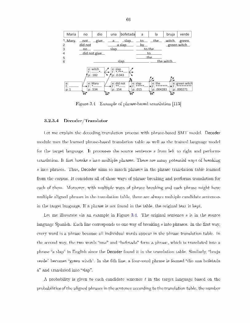
66

Maria no dio una bofetada a la bruja verde

Mary not give a slap to the witch greendid4not 4 a4slap4 by green4witch

no slap to4thedid4not4give to

theslap the4witch

e:4witchf4:4-------*-p:4.182

e:4slapf4:4*-***----p:4.0.043

e:4Maryf4:4*--------p:4.534

e:4did4notf4:4**------p:4.154

e:4slapf4:4*****----p:4.015

e:4thef4:4*******--p:4.004283

e:4green4witchf4:4*********p:4.000271

e:4f:4 ---------p:41

1

234

56

Figure 3.4 Example of phrase-based translation [113]

3.2.3.4 Decoder/Translator

Let me explain the decoding/translation process with phrase-based SMT model. Decoder

module uses the learned phrase-based translation table as well as the trained language model

for the target language. It processes the source sentence s from left to right and performs

translation. It �rst breaks s into multiple phrases. There are many potential ways of breaking

s into phrases. Thus, Decoder aims to match phrases in the phrase translation table learned

from the corpus. It considers all of those ways of phrase breaking and performs translation for

each of them. Moreover, with multiple ways of phrase breaking and each phrase might have

multiple aligned phrases in the translation table, there are always multiple candidate sentences

in the target language. If a phrase is not found in the table, the original text is kept.

Let me illustrate via an example in Figure 3.4. The original sentence s is in the source

language Spanish. Each line corresponds to one way of breaking s into phrases. In the �rst way,

every word is a phrase because all individual words appear in the phrase translation table. In

the second way, the two words �una� and �bofetada� form a phrase, which is translated into a

phrase �a slap� in English since the Decoder found it in the translation table. Similarly, �bruja

verde� becomes �green witch�. In the 6th line, a four-word phrase is formed �dio una bofetada

a� and translated into �slap�.

A probability is given to each candidate sentence t in the target language based on the

probabilities of the aligned phrases in the sentence according to the translation table, the number

67

of translated words in s, as well as based on the probability P (t) of the sentence t according to

the language model. The probability for a candidate sentence is gradually computed along the

translation/decoding process. For example, after the word �Maria� is translated into �Mary�,

the current probability is 0.534. However, it decreases to 0.154 when the current text is �Mary

did not�, and so on. The sentence with the highest probability is presented.

3.2.3.5 Implication/Applications

Statistical machine translation has been successfully used in NLP and in real application

(Google's Translate, etc.) where text in one language (e.g. French) is translated to correspond-

ing text in another language (e.g. English). The advantage of such SMT model is that it does

not need manual encoding of translation rules. It uses EM algorithm to automatically learn

rules and apply them for translation, hence it do not need heuristics like name similarity to

detect mapping rules.

We can use it for corresponding translation source code from one language (e.g. Java) to

another language (e.g. C#), or from natural language (e.g. English) to a programming language

(e.g. Java). The ability to statistically learn mapping rules without heuristics is very promising,

especially when manual encoding of mappings is tedious and sometimes infeasible. I will discuss

the applications based on SMT in 6.2 and 6.3.

3.3 Topic Models for Software

3.3.1 Topic Model for Source Code (S-Component)

S-component in our model is adopted from LDA [28]. In general, source code always includes

program elements and are written in some speci�c programming language. In our model, a

source �le is considered as a text document s. Texts from the comments and identi�ers in a

source �le are extracted to form the words of the document s.

Topic vector. A source document s has Ns words. In S-component, each of the Ns positions

in document s is considered to describe one speci�c technical topic. Therefore, for each source

68

document s, we have a topic vector zs with the length of Ns in which each element of the

vector is an index to one topic (i.e. 1-K).

Topic Proportion. Each position in s describes one topic, thus, the entire source document s

can describe multiple topics. To represent the existence and importance of multiple topics in

a document s, LDA introduces the topic proportion θs. θs for each document s is represented

by a vector with K elements. Each element corresponds to a topic. The value of each element

of that vector is a number in [0-1], which represents the proportion of the corresponding topic

in s. The higher the value θs[k] is, the more important topic k contributes to the document

s. For example, in the �le InteropService.java, if θs = [0.4, 0.4, 0.1, ...], 40% of words are about

outgoing sync, other 40% are about incoming sync, etc.

Vocabulary and Word Selection. Each position in source code document s is about one topic.

However, to describe that topic, one might use di�erent words which are drawn from a vocab-

ulary of all the words in the project (and other regular words in any dictionary of a natural

language). Let me call the combined vocabulary V oc with the size of V . Each word in V oc

has a di�erent usage frequency for describing a topic k, and a topic can be described by one

or multiple words. LDA uses a word-selection vector φk for the topic k. That vector has the

size of V in which each element represents the usage frequency of the corresponding word at

that element's position in V oc to describe the topic k. Each element v in φk can have a value

from 0 to 1. For example, for a topic k, φk = [0.3, 0.2, 0.4, ...]. That is, in 30% of the cases the

�rst word in V oc is used to describe the topic k, 20% of the cases the second word is used to

describe k, and so on. For a software system, each topic k has its own vector φk then K topics

can be represented by a K × V matrix φsrc, which is called per-topic word distribution. Note

that φsrc is applicable for all source �les, rather than for s individually.

LDA is a machine learning model and from its generative point of view, a source �le s in

the system is considered as an �instance� generated by a �machine� with three aforementioned

variables zs, θs, φsrc. Given a source code document s of size Ns, based on topic proportion θs of

the document, the machine generates the vector zs describing the topic of every position in the

document s. For each position, it then generates a word ws based on the topic assigned to that

69

position and the per-topic word distribution φsrc corresponding to that topic. This is called a

generative process. The terms in the source �les in the project's history are the observed data.

One can train the LDA model with historical data to derive those three parameters to �t the

best with the observed data. As a new document s′ comes, LDA uses the learned parameters

to derive the topics of the document and the proportion of those topics.

3.3.1.1 Topic Model for Bug Report (B-Component)

Let me describe the B-component, which is extended from LDA [28]. As a consequence

of an incorrect implementation of some technical aspects in the system, a bug report is �led.

Thus, a bug report describes the buggy technical topic(s) in a system. Similar to S-component,

B-component also considers each bug report b as a document with three variables zb, θb, φBR.

A bug report b has Nb words. The topic at each position in b is described by a topic vector zb.

The selection for the word at each position is modeled by the per-topic word distribution φBR.

Note that φBR applies to all bug reports and it is di�erent from φsrc.

The bug report b has its own topic proportion θb. However, that report is in�uenced not only

by its own topic distribution, but also by the topic distribution parameters of the buggy source

�les corresponding to that bug report. The rationale behind this design is that in addition to its

own topics, the contents of a bug report must also describe about the occurrence of the bug(s).

That is, the technical topics of the corresponding buggy �les must be mentioned in the bug

report. At the same time, a bug report might describe about other relevant technical aspects

in the system from the point of view of the bug reporter.

Let me use s1, s2, ..., sM to denote the (buggy) source �les that are relevant to a bug report

b. The topic distribution of b is a combination of its own topic distribution θb (from the

writing view of a bug reporter) and topic distributions of s1, s2, ..., sM . In BugScout, we have

θ∗b = θs1.θs2.....θsM .θb. The equation represents the sharing of buggy topics in a bug report and

corresponding source �les. If a topic k has a high proportion in all θs and θb (i.e. k is a shared

buggy topic), it also has a high proportion in θ∗b . The generative process in B-component

is similar to S-component except that it takes into account the combined topic proportion

θ∗b = θs1.θs2.....θsM .θb.

70

File.new

g

1C (g)

FileWriter.�ush

FileWriter.�ush

2C (g) List.add

File.new

FileWriter.new

FileWriter.append

FileWriter.close

List.get

1P (g)

2P (g)

FileWriter.new

FileWriter.append

List.get

FileWriter.close

File.new

FileWriter.new

FileWriter.append

FileWriter.close

List.get

File.new

FileWriter.new

FileWriter.append

List.get

FileWriter.close

File.new

FileWriter.new

FileWriter.append

List.get

FileWriter.close

List.add

Figure 3.5 Parent and Children Graphs

3.4 Deterministic Pattern-based Model

3.4.1 Groum - Graph-based Representation of API Usage

3.4.1.1 API Usage Representation

De�nition 3.4.1 ( API Usage) An API usage is a set of related API elements (i.e., classes,

method calls, �eld accesses, and operators) in use in the client code, together with control

units (i.e., condition and repetition) in a speci�c order, and with the control and data �ow

dependencies among API elements [166].

In our prior work [176], we developed a graph-based representation model, called Groum to

represent API usages.

De�nition 3.4.2 ( Groum [176]) A Groum is a graph in which the nodes represent actions

(i.e., method calls, overloaded operators, and �eld accesses) and control points (i.e., branching

points of control units if, while, for, etc.). The edges represent the control and data �ow

dependencies between nodes. The nodes' labels are from the names of classes, methods, or

control units.

71

1 Display display = new Display();2 Shell shell = new Shell( display ) ;3 ...4 Button button = new Button(shell, SWT.PUSH);5 button.setText("OK");6 button. setSize (new Point(40,20));7 button. setLocation(new Point(200,20));8 ...9 shell .pack();10 shell .open();11 while (! shell . isDisposed ()) {12 if (! display .readAndDispatch())13 display . sleep () ;14 }15 display . dispose () ;

Figure 3.6 SWT Usage Example 1

My colleages' previous work [176] shows that an API usage can be represented by a connected

(sub)graph in a Groum. In Figure 3.5, P2(g) illustrates the pattern on FileWriter as a Groum.

The action nodes such as File.new, FileWriter.new, etc. represent API calls, �eld accesses, or

operators. The nodes' labels have fully quali�ed names and an action node for a method call also

has its parameters' types (not shown). An edge connects two action nodes if there exist control

and data �ow dependencies between them. For example, FileWriter.new must be executed before

FileWriter.append and the object created by the former is used in the latter call, thus, there is

an edge from the former to the latter. If a usage involves a while loop , a control node named

WHILE is created after the node for the condition and is connected to the �rst node in the body

of while. If a method call is an argument of another call, e.g., m(n()), the node for the call in

the argument will be created before the node for the outside method call (i.e., the node for n

comes before that of m). The rationale is that n is evaluated before m.

3.4.2 Deterministic Pattern-based Model with Groum

De�nition 3.4.3 ( Pattern) An API usage pattern is a set of API elements (i.e. classes/-

variables/method calls) and control structures (i.e. condition/repetition) with speci�c control

and data dependencies. A usage pattern speci�es a correct usage of API elements to perform a

programming task.

72

Display.new

Shell.new

Shell.pack

Shell.open

Shell.isDisposed

Display.readAndDispatch

Display.sleep

Display.dispose

IF

WHILE

Display Shell

datadependency control dependency

data node

action node

control node

Button.new

Button.setText

Button.setSize

Button.setLocation

Button

Button.new

Button.setText

Button

Button.setLayoutData

FormData.new FormData

a. b.

c.

Figure 3.7 SWT Usage Patterns

Figure 3.6 (lines 1-2, 9-15) shows an instance of SWT window creation pattern. An instance

is concrete code realizing that pattern. A pattern contains the usage of the classes (via variables),

methods (via method calls), and control structures (e.g. while, if), with speci�c orders and

inter-dependencies. A pattern could be a composite one built from multiple sub-patterns. The

patterns could be interleaved with each other.

De�nition 3.4.4 ( Feature) A graph-based feature is a sequence of the textual labels of the

nodes along a path of a Groum. A token-based feature is a lexical token extracted in a query.

The size of a graph-based feature is de�ned as the number of elements in its corresponding

sequence. Thus, in a Groum, a node has a corresponding graph-based feature of size 1, and an

edge has a graph-based feature of size 2. Larger features can be built from a path in the Groum.

In Figure 5.6a, there are a size-1 graph-based feature [Shell.new], a size-2 graph-based feature

[Shell.new, Shell.pack], a size-3 graph-based feature [Shell.pack, Shell.open, Shell.isDisposed], etc.

In our model, a token-based feature always has its size equal to 1 and is used to represent

the usage of a class, a method, or a control structure in the current (incomplete) code. For

example, the query for (Iterator _ is incomplete and can not be parsed into an AST. However,

73

Score(lex=”next”)

Scorelex Scoresyn Scoresem

Hidden layers

0..0010 1..0000 0..0100 000..10 …… …… …… 0010..0 …… …… ……

while ( iter hasNext next WHILE OP EXP EXP Keyword Var[Iterator,..]Call[Scaner, hasNext,

0, boolean]Var[Iterator,..]

n-1 previous lexemes

+

n-1 previous syntaxemes n-1 previous sememes

iter

0..0100

DNNlex DNNsyn DNNsem

Figure 3.8 Context-aware DNN-based Model: Incorporating Syntactic and Semantic Contexts

our model still extracts two tokens for and Iterator, and uses them to match this query to the

patterns that have the usages with a for loop and an Iterator variable.

To measure the similarity of any two features, our model de�nes a function sim that com-

pares their textual similarity and the orders of their elements.

To compare a query against a pattern via features, our model also takes into account the

context information of the query. Such information is modeled via the context-sensitive weights

associated with the features. That is, context-sensitive weights measure the signi�cance of the

features in a query based on the relations of the features to the focus editing position (user-based

factor) and based on the structure of the query's Groum (structure-based factor).

3.5 Deep Neural Network-based Models

3.5.1 DNN Models for Language Models

3.5.1.1 Overview and Key Ideas

In this section, I introduce Dnn4C, a DNN-based LM for source code, that complements

the local history of n-gram by additionally incorporating syntactic and semantic contexts. The

work adapted Huang et al. [88]'s model for our new code features listed in Section 3:

1. Syntaxeme and sememe sequences as contexts. While existing deep learning LMs

use only lexical code tokens with limited contexts, we also attempt to parse the current �le

and derive the syntaxeme and sememe sequences for those tokens (if possible), and use those

74

sequences as contexts. We expect that with information on the current syntactic unit and

data/token types, Dnn4C is able to capture patterns at higher abstraction levels, thus, leading

to more correct suggestion. For example, in Figure 3.8, with the token hasNext and the sememe

CALL [Scanner, hasNext, 0, boolean] being in the contexts, Dnn4C could rank the token next of

Scanner higher since hasNext of a Scanner object is often followed by a call to next.

2. Multiple-prototype model (DNNs). Instead of using only one DNN for all sequences

at three levels, we input each lexeme and its syntax and semantic contexts into two additional

DNNs (Figure 3.8), each of which is dedicated to incorporate one type of context. When word

meaning is still ambiguous given local context, we expect that information in other contexts can

help disambiguation [88]. As shown in Huang et al. [88], using a single DNN would not capture

well di�erent meanings of a word in di�erent contexts as the model is in�uenced by all of its

meanings. They empirically showed that using multiple DNNs for multiple representations in

di�erent contexts capture well di�erent senses and usages of a word.

3. Training objectives. There are following objectives in training for Dnn4C: 1) to train

the �rst DNN to learn to determine the potential next code token based on the n-1 previous

lexemes, and 2) to train the two additional DNNs for contexts to discriminate each correct

next token c from other tokens in the vocabulary given the window of n-1 previous lexemes

and the syntactic/semantic contexts of that token c. That is, the score should be large for

the actual next token, compared to the score for other tokens. Speci�cally, let us have the

current sequence lex of n-1 prior lexemes. We aim to train Dnn4C to discriminate the actual

next token c (appearing after lex) from the other tokens in the vocabulary. Let Scoresyn and

Scoresem be the scoring functions for two DNNs modeling syntactic and semantic contexts.

We aim that with the input lex, they give the scores Scoresyn(c, syn) and Scoresem(c, sem)

for the correct token c much higher than the scores Scoresyn(c′, syn) and Scoresem(c′, sem) for

any other token c′ in the vocabulary. syn and sem are the sequences of n-1 prior syntaxemes

and n-1 prior sememes representing the contexts for c and lex. In general, one can use any

subsequences of the syntaxeme and sememe sequences for the tokens from the beginning of a

�le to c as contexts. However, performance will be an issue when the lengths of those sequences

are large. Thus, we used the same length (n-1) for syntaxeme and sememe sequences.

75

As an example, we want to have the scores Scoresyn and Scoresem for the token next of

Scanner to be higher than the scores for other tokens. Mathematically, as suggested in [88, 43],

we use the following training objective O(c, syn) that minimizes the ranking loss for each pair

of token c and sequence syn in a �le, and gives the margin of 1 between two such scores. For

the sequence lex ending with c:

O(c, syn) =∑c′∈V

max(0, 1− (Scoresyn(c, syn)− Scoresyn(c′, syn))) (3.10)

If the margin between the two scores for c and c′ is greater than 1, the max function returns 0,

helping the objective O reach its minimum. If the margin is smaller than 1, the 2nd argument

in the max function is greater than 0. Thus, by using the max function, we aim to minimize

that ranking loss for (c, syn). The same training objectives O(c, lex) and O(c, sem) are used

for lexeme and sememe sequences. Note: the projection layer could be used in each DNN (not

shown).

3.5.1.2 Model Architecture and Details

Figure 3.9 shows Dnn4C's architecture. It takes as input 3 di�erent input levels of lexemes,

syntaxemes, and sememes to predict the next lexeme. For training, for each sequence s of

length n, the correct lexeme c at the nth position of s is fed into the input lexn, which is

also fed into 3 DNNs for 3 levels (Figure 3.8). Three sequences of length n-1 for lexemes,

syntaxemes, and sememes corresponding to s are fed into the other inputs. For predicting, each

candidate c in the lexeme vocabulary is fed into the input lexn and Score(c) is computed and

normalized (representing how likely c is the next token of the input sequence lex1, ..., lexn−1).

All candidates c are ranked based on their scores. Details on training/predicting are given later.

Lexical level. The input at this level is the concatenated discrete feature vectors of n-1 prior

lexemes lex1, ..., lexn−1 of the current lexn. Each lexeme is represented by a vector where only

the index of that lexeme is one. The role of projection for lexemes is for word embedding, i.e.,

to map each lexeme to a continuous feature space:

h1(y) = tanh

|V |∑x=1

wp(x, y)i(x) + bp(y)

,∀y = 1, · · · ,M1 (3.11)

76

0

0

010

00

01

0

10

00

0

lex1

lex2

lexn-1

Lexical level

Projection

Syntactic levelsyn1

synn-1

syn2

Semantic levelsem1

semn-1

sem2

lexn

Sco

relex

Sco

resyn

Sco

resem

+ score(lexn=wi)

———————

∑score(lexn=wi)

Syntactic-and-semantic-

context-aware DNN

wi

Figure 3.9 Dnn4C: Deep Neural Network Language Model for Code

i(x) is the value of node x at the input; h1(y) is the output value of node y in this projection

layer; wp(x, y) is the weight of the connection from input x to output y, and bp(y) is a bias

value for node y; M1 is the number of outputs of this layer; and V is the vocabulary.

Then, the output feature vectors of this layer for n-1 prior lexemes are concatenated with

lexn: h1 = [h1(1); ...;h1(M1); lexn]. To compute the score of a node y at the lexical level, we

have:

lex(y) = tanh

(n∑x=1

wlex(x, y)h1(x) + blex(y)

),∀y = 1, · · · ,Mlex

Scorelex =

Mlex∑y=1

w′lex(y)lex(y) + b′lex

(3.12)

where wlex and w′lex are the weights at the lexical level. blex(y) and b′lex are the bias values for

node y at this level.

Syntactic level. For the score from the DNN for syntactic context, we use the sequence of n-1

prior syntaxemes syn1, ..., synn−1 as context, assuming that synn is the syntaxeme for lexn. A

lexeme corresponds to only one syntaxeme, but a syntaxeme can have multiple lexemes. Each

77

syntaxeme is represented by a vector where only the index of that syntaxeme in the vocabulary

is set to 1, while all others are 0s. To form the syntactic context, we concatenate the vectors of

n-1 syntaxemes with the vector of the lexical token lexn right after the current lexical sequence

lex1, lex2, ..., lexn−1. Thus, we have the combined vector synh = [syn1, syn2, ..., synn−1, lexn].

To compute the score for a node y at the syntactic level, we use:

syn(y) = tanh

(n∑x=1

wsyn(x, y)synh(x) + bsyn(y)

),∀y = 1, · · · ,Msyn

Scoresyn =

Msyn∑y=1

w′syn(y)syn(y) + b′syn

(3.13)

where wsyn and w′syn are the weights at the syntactic level. bsyn(y) and b′syn are the bias values

for a node y at this level.

During training, several combined vectors will be formed by replacing lexn with several

other words in the lexical vocabulary. The training objective is to minimize O(lexn, syn),

i.e., the ranking loss for each pair of token lexn and sequence syn (Section 3.5.1.1). Note

that, in formula (1), Scoresyn(c, syn) is equal to Scoresyn in formula (3) where c = lexn and

syn = [syn1, ..., synn−1].

Semantic level. To compute the score from the DNN for semantic context, we perform a

similar process as the one at the syntactic level, except that the syntaxemes are replaced by the

sememes of the current lexical sequence. That is, from the combined vector for the semantic

context, semh = [sem1, sem2, ..., semn−1, lexn], we compute sem(y) and Scoresem as in (3).

The number of hidden nodes is Msem. The weights will be learned via training as well.

Similarly, the training objective is to minimize the ranking loss O(lexn, sem) for each pair

of token lexn and sequence sem.

Final score. The �nal score for each lexical token wi is the normalized one of the sum of all

three scores over all possible wi in V .

Training. We �rst parse each �le in the training corpus to produce lexeme, syntaxeme, and se-

meme sequences. We collect all sequences of lexemes with a �xed length n: [lex1, lex2, ..., lexn].

The corresponding syntaxeme synn−1 and sememe semn−1 of lexn−1 are identi�ed. We then col-

lect n-1 prior units of lexemes lex = [lex1, lex2, ..., lexn−1], syntaxemes syn = [syn1, syn2, ..., synn−1]

78

and sememes sem = [sem1, sem2, ..., semn−1], and use them as input to Dnn4C in Figure 3.9.

The token lexn is used as the correct next token and fed into the input labeled lexn. The score

for that token is computed with the current weights (weights are initialized in the beginning).

Then, Dnn4C randomly selects a lexical token c′ (di�erent from lexn) as a negative example for

the pair (lexn, lex), and feeds it into the input labeled lexn (instead of using the correct token

lexn). The score Score(c′, lex) is computed. The di�erence of the scores Score(lexn, lex) and

Score(c′, lex) is recorded. Then, the weights are updated for DNNlex to minimize the value of

the objective O(lexn, lex) by taking a gradient step with respect to this choice c′. That is, we

take the derivative of the ranking loss with respect to the weights of the DNN as in training

for Huang's model [88]. Dnn4C repeats the process for other token c′′ in the lexeme vocabulary

until reaching a certain number of iterations. As suggested in [88], when there is su�ciently

large number of iterations, the quality is as good as using stochastic gradient descent. The

training process continues in the same way to train the weights for the two other DNNs for

syntaxemes and sememes except that we use Score(lexn, syn) and Score(lexn, sem). Details

on this type of objective of minimizing ranking loss can be found in [43].

Prediction. At a point L of suggestion in a program, we process the code using PPA [45] to

construct the sequences of syntaxemes and sememes up to L. For a �xed value of n, we collect

n-1 prior lexemes, syntaxemes, and sememes (from the last token before L) and use them as

the input of Dnn4C. Then, each token c in the vocabulary V will be fed into the input labeled

lexn in Figure 3.9. The score for c is computed/normalized to show how likely the next token

is c.

3.6 Graph-based Model

3.6.1 Bayesian-based Generation Model

Let me present GraLan, a graph-based statistical language model, in the context of its

application of API code suggestion where it is applied to the graphs representing API usages.

However, GraLan is general for any graphs extracted from code. For the concepts speci�cally

applicable to API suggestion, we will explicitly state so.

79

3.6.1.1 API Usage Representation

De�nition 3.6.1 ( API Usage) An API usage is a set of related API elements (i.e., classes,

method calls, �eld accesses, and operators) in use in the client code, together with control

units (i.e., condition and repetition) in a speci�c order, and with the control and data �ow

dependencies among API elements [166].

In prior work [176], my collaborators developed a graph-based representation model, called

Groum to represent API usages.

De�nition 3.6.2 ( Groum [176]) A Groum is a graph in which the nodes represent actions

(i.e., method calls, overloaded operators, and �eld accesses) and control points (i.e., branching

points of control units if, while, for, etc.). The edges represent the control and data �ow

dependencies between nodes. The nodes' labels are from the names of classes, methods, or

control units.

Prior work [176] shows that an API usage can be represented by a connected (sub)graph in

a Groum. In Figure 3.10, P2(g) illustrates the pattern on FileWriter as a Groum. The action

nodes such as File.new, FileWriter.new, etc. represent API calls, �eld accesses, or operators.

The nodes' labels have fully quali�ed names and an action node for a method call also has its

parameters' types (not shown). An edge connects two action nodes if there exist control and

data �ow dependencies between them. For example, FileWriter.new must be executed before

FileWriter.append and the object created by the former is used in the latter call, thus, there is

an edge from the former to the latter. If a usage involves a while loop, a control node named

WHILE is created after the node for the condition and is connected to the �rst node in the body

of while. If a method call is an argument of another call, e.g., m(n()), the node for the call in

the argument will be created before the node for the outside method call (i.e., the node for n

comes before that of m). The rationale is that n is evaluated before m.

80

File.new

g

1C (g)

FileWriter.�ush

FileWriter.�ush

2C (g) List.add

File.new

FileWriter.new

FileWriter.append

FileWriter.close

List.get

1P (g)

2P (g)

FileWriter.new

FileWriter.append

List.get

FileWriter.close

File.new

FileWriter.new

FileWriter.append

FileWriter.close

List.get

File.new

FileWriter.new

FileWriter.append

List.get

FileWriter.close

File.new

FileWriter.new

FileWriter.append

List.get

FileWriter.close

List.add

Figure 3.10 Parent and Children Graphs

3.6.1.2 Generation Process

A graph can be constructed from one of its subgraphs by adding nodes and edges. Thus,

the graph generation process can be modeled by the addition of nodes and edges to already-

constructed subgraphs. Thus, we de�ne the following concept:

De�nition 3.6.3 ( Parent and Children Graphs) A connected graph P (g) is a parent graph

of a graph g if adding a new node N and inducing edges from N to P (g) will create g. g is a

child graph of P (g). A child graph of g is denoted as C(g). A graph can have multiple parents

and multiple children.

This relation is general for any graph. However, let me illustrate it via Figure 3.10 for

API usage graphs (Groums). The graph P1(g) is a parent graph of g because adding the node

File.new and the edge File.new-FileWriter.new to P1(g) will create g. g also has its children C1(g)

and C2(g). The suggestion of a new API given an already-observed Groum g can be done by

81

considering all of its children C(g)′s. We extend the concept of parents to ancestors and that

of children to descendants.

De�nition 3.6.4 ( Context) The context of a generation process of a new graph C(g) from

a graph g is a set of graphs including g that are used to generate C(g).

We use Pr(C(g)|Ctxt)=Pr((g,N+, E+)|Ctxt) to denote such generation probability. N+

is the additional node and E+ is the list of additional edges connecting g and N+ to build

C(g). All the graphs in Ctxt including g a�ects the generation of C(g). For the API suggestion

application, the context contains the subgraphs g1, .., gn (of the Groum G built from the code)

that surround the current editing location. Those subgraphs represent the potential usages

that are useful in the prediction. For each child graph generated from a subgraph gi, the

corresponding additional nodes Nj 's will be collected

and ranked. Each new node will be added to G to produce a candidate graph G′ as a suggestion

(see details in Section 5.3.2).

82

CHAPTER 4. APPLICATIONS: FINDING LINKING BETWEEN

SOFTWARE ARTIFACTS

4.1 Bug Localization

4.1.1 Problem Statement

To ensure software integrity and quality, developers always spend a large amount of time

on debugging and �xing software defects. A software defect, which is informally called a bug, is

found and often reported in a bug report. A bug report is a document that is submitted by a

developer, tester, or end-user of a system. It describes the defect(s) under reporting.

Such documents generally describe the situations in which the software does not behave as

it is expected, i.e. fails to follow the technical requirements of the system. Being assigned to �x

a bug report, a developer will analyze the bug(s), search through the program's code to locate

the potential defective/buggy �les. Let me call this process bug �le localization.

This process is crucial for the later bug �xing process. However, in a large system, this

process could be overwhelming due to the large number of its source �les. At the same time, a

developer has to leverage much information from the descriptive contents of the bug report itself,

from his domain knowledge of the system and source code, from the connections between such

textual descriptions in a report and di�erent modules in the system, and from the knowledge

on prior resolved bugs in the past, etc. Therefore, to help developers target their e�orts on the

right �les and raise their e�ectiveness and e�ciency in �nding and �xing bugs, an automated

tool is desirable to help developers to narrow the search space of buggy �les for a given bug

report.

In this section, I introduce BugScout, a topic-based approach to locate the candidates of

buggy �les for a given bug report.

83

α

θsM+1 θsM

θs1... θ

b

zsM+1 sM

s1...

bz z z

sM+1 sM

s1 bw ...w w w

φBRφ

srcφsrc

φsrc

β

...

Figure 4.1 BugScout Model

4.1.2 Approach using Topic Model

Sections 3.3.1.1 and 3.3.1 describe topic models for bug-reports and source code. In this

section, I will describe how to combine those two models for bug localization model.

4.1.2.1 BugScout Model

The approach models the relation between a bug report and corresponding buggy source �les

by combining the S-component 3.3.1 and B-component 3.3.1.1 into BugScout (Figure 4.1). For

a bug report b, in the B-component side, there are 3 variables that control b: zb, θb, and φBR.

However, if the source �les s1, s2, ..., sM are determined to cause a bug reported in bug report

b, the topic vector zb will be in�uenced by the topic distributions of those source �les. That

is, there are links from θs1 , θs2 , ...θsM to zb. For each source document, there are 3 variables

that control s: zs, θs, and φsrc (Figure 4.1). There are two hyper parameters α and β whose

conditional distributions are assumed as in LDA. α is the parameter of the uniform Dirichlet

84

prior on topic distributions θs and θb. β is the parameter of the uniform Dirichlet prior on the

per-topic word distributions φsrc and φBR.

For training, the model will be trained from historical data including source �les, bug re-

ports and the links between bug reports and corresponding �xed source �les. The variables of

BugScout will be trained to derive its parameters and to make the model �t most with both

the document data and the links between bug reports and corresponding buggy source �les.

For predicting, the model will be applied to a new bug report bnew. BugScout uses its

trained parameters to �generate� that bug report and estimate its topic proportion θbnew . That

topic proportion will be used to �nd corresponding source �les that share most topics. Cosine

distance is used to determine the topic proportion similarity. We use sim(s, b) to denote the

topic proportion similarity between a source �le s and a bug report b. The topics of that bug

report are compared with the topics of all source �les. Finally, the �les that have shared the

buggy topics with the new bug report will be ranked and recommended to the developers.

Because BugScout has two components and the dependencies among variables in the internal

model become much di�erent from LDA, we developed our own algorithms for training BugScout

with historical data and predicting for a new bug report. We will present them in Section 4.1.2.

Integrating with Defect-Proneness of Source Files: In a software system, some �les

might be more buggy than the others. We integrate this characteristic into BugScout to improve

its accuracy in buggy �le prediction. We use the following equation to formulate the idea:

P (s|b) = P (s) ∗ sim(s, b) (4.1)

In the equation, P (s|b) is the total relevance measure of a source �le to a given bug report b.

sim(s, b) is the similarity of the topics of the source �le and those of the bug report. P (s) is

the bug pro�le of source �le s. In BugScout's current implementation, P (s) is determined by

the number of bugs in the �le s in the history and by its size. Other strategies for computing

defect-proness of a source �le can be used for P (s).

The equation implies the inclusion of both defect-proneness and the buggy topics of a source

�le. Given a new bug report, if a source �le is determined as having higher buggy potential,

85

and it also contains shared buggy topics with the bug report, it will be ranked higher in the list

of possible buggy �les. Next section will describe our training and predicting algorithms.

4.1.2.2 Training Algorithm

The goal of this algorithm is to estimate BugScout's parameters given the training data

from a software system. The collection of source �les S, that of bug reports B, and the set of

links Ls(b) between a bug report and corresponding source �le(s) will be used to train BugScout

and estimate its parameters (zs, θs, φsrc), and (zb, θb, φBR).

Algorithm Overview. Our algorithm is based on Gibbs sampling method [71]. The idea of

Gibbs sampling is to estimate the parameters based on the distribution calculated from other

sampled values. The estimation is made iteratively between the values until the estimated

parameters reach their convergent state (i.e. the new estimated value of a parameter do not

change in comparison with its previous estimated value).

Figure 4.2 shows the pseudo-code of our training algorithm. Function TrainModel() is used

to train BugScout by using the collections of source �les (S), bug reports (B) and the set of links

Ls(b) between the bug reports and the corresponding buggy source �les. Line 3 describes the

initial step where the parameters zs, zb, φsrc, φBR are assigned with randomly values. Lines 4-22

describe the iterative steps in estimating the parameters using Gibbs sampling. The iterative

process terminates when the values of parameters are convergent. The convergent condition

is determined by checking whether the di�erence between the current estimated values and

previous estimated ones is smaller than a threshold. In our implementation, the process is

stopped after a number of iterations, which is large enough to ensure a small error. In each

iteration, the parameters are estimated for all source code documents s in S (lines 7-13) and

all bug reports b in B (lines 15-21).

Detailed Description. Let me explain in details all the steps.

Step 1: Estimating the topic assignment for source documents in S (lines 7-10). With each

document s in S, BugScout estimates the topic assignment zs[i] for position i (line 9). Function

EstimateZS (lines 26-31) provides the detailed computation. For each topic k in K topics,

86

1 // −−−−−−−−−−−−−−− Training −−−−−−−−−−−−−−−−−2 function TrainModel(SourceFiles S, BugReports B, Links Ls(b))3 zS , zB , φsrc, φBR ← random();4 repeat5 z′S ← zS , z

′B ← zB

6 // Update the variables for source documents7 for (SourceFile s ∈ S)8 for (i = 1 to Ns)9 zs[i] = EstimateZS(s, i) //estimate topic assignment at position i10 end11 θs[k] = Ns[k]/Ns //estimate topic distribution12 end13 φsrc,k[wi] = Nk[wi]/N //estimate per−topic word distribution14 // Update the variables for bug reports15 for (BugReports b ∈ B)16 for (i = 1 to Nb)17 zb = EstimateZB1(wb, Ls(b), i)18 end19 θb[k] = Nb[k]/Nb20 end21 φBR,k[wi] = Nk[wi]/N22 until (|z − z′| <= ε)23 return zS , zB , θS , θB , φsrc, φBR24 end25 // −−−−−−−−− Estimate topic assignment for s −−−−−−−26 function EstimateZS(SourceFile ws, int i)27 for (k = 1 to K)

28 p(zs[i] = k)← (ns[−i,k]+α)(ns−1+Kα)

(nsrc,k[−i,wi]+β)

(nsrc,k−1+V β)

29 end30 zs[i]← sample(p(zs[i]))31 end32 // −−−−−−−−− Estimate topic assignment for b −−−−−−−33 function EstimateZB1(BugReport wb, int i, Links Lws (wb))34 for (k = 1 to K)

35 p(zb[i] = k)←

(nb[−i,k]∏

s∈Ls(b)

ns[k] + α)

((nb−1)

∏s∈Ls(b)

ns +Kα)

(nBR,k[−i,wi]+β)

(nBR,k−1+V β)

36 end37 zb[i]← sample(p(zb[i]))38 end

Figure 4.2 Model Training Algorithm

BugScout estimates the probability that topic k will be assigned for position i in document s.

Then, it samples a topic based on the probabilities of ks (line 30). The equation follows the

topic assignment estimation by Gibbs sampling in LDA [71]:

p(zi = k|zs[−i], ws) =(ns[−i, k] + α)

(ns − 1 +Kα)

(nsrc,k[−i, wi] + β)

(nsrc,k − 1 + V β)(4.2)

where ns[−i, k] is the number of words in s (except for the current position i) that are assigned

to topic k; ns is the total number of words in s; nsrc,k[−i, wi] is the number of words wi in all

source documents S (except for the current position) that are assigned to topic k; and nsrc,k is

the number of all words in S that are assigned to topic k.

87

The intuition behind this equation is that, given a word ws[i] at position i of document s,

the probability a topic k that is assigned to that position can be estimated based on both the

proportion of the terms in s (excluding the current one) that describe topic k (i.e. (ns[−i,k])(ns−1) )

and the probability that the current term ws[i] appears if topic k is assigned (i.e. (nsrc,k[−i,wi])(nsrc,k−1) ).

Moreover, the current position value can be estimated by prior knowledge of surrounding posi-

tions.

Step 2: Estimating topic proportion θs for a source �le (line 11). Line 11 shows the estimation

for the topic proportion of source �le s. Once topic assignments for all positions in s are

estimated, the topic proportion θs[k] of topic k in that document can be approximated by

simply calculating the ratio between the number of words describing the topic k and the length

of the document.

Step 3: Estimating word distribution φsrc (line 13). Line 13 shows the estimation for the

per-topic word distribution for each word wi from V oc (size V ) and topic k. φsrc,k is a vector of

size V representing how often each word in vocabulary V oc can be used to describe topic k in

the source �le collection S. Element at index i in φk determines how often the word with index

i in V oc can be used to describe k. Thus, φk[wi] can be approximated by the ratio between the

number of times that the word index i in V oc is used to describe topic k and the total number

of times that any word that is used to describe k.

Step 4: Estimating the topic assignment for bug reports in B (lines 16-18). For each bug

report b in B, BugScout estimates the topic assignment zb[i] for position i (line 17). Function

EstimateZB1() (lines 33-38) provides the detail. For each topic k in K, BugScout estimates the

probability that topic k will be assigned for position i. It then samples a topic based on the

probabilities of ks (line 37). The estimate equation is similar to that for a source �le document:

p(zb[i] = k|zb[−i], wb) =(n∗b [−i, k] + α)

(n∗b [−i] +Kα)

(nBR,k[−i, wi] + β)

(nBR,k − 1 + V β)(4.3)

where nBR,k[−i, wi] is the number of words wi in all bug reports in B, except the current

position, that are assigned to topic k, and nBR,k is the number of words in S describing k.

88

The crucial di�erence between (4.3) and (4.2) is that because a bug report describes the

buggy topic(s) in the corresponding source documents, the proportion θ∗ of a topic k described

in the bug report includes its own topic proportion θb and the topic proportions of corresponding

source �les θs1 , θs2 , ..., θsM , where s1, s2, ..., sM ∈ Ls(b) (i.e. the set of buggy source �les linking

to bug report b). That leads to n∗b [−i, k] = nb[−i, k]∏

s∈Ls(b)

ns[k] and

n∗b [−i] = (nb − 1)∏

s∈Ls(b)

ns, in which nb[−i, k] is the number of words in b (except for the

current position i) that are assigned to topic k. nb is the total number of words in b. For each

buggy source document s linked to b, ns[k] is the number of words in s (except for the current

position i) that are assigned to topic k. ns is the total number of words in s.

Step 5: Estimating topic proportion θb for a bug report b and estimate word distribution φBR

(line 19 and line 21). Those estimation steps are similar to the steps for θs and φsrc.

4.1.2.3 Predicting and Recommending Algorithm

The goal of this algorithm is to estimate the topic proportion of a newly arrived bug report

bnew and derive a candidate list of potential buggy source �les that cause the reported bug(s).

The algorithm uses the trained model from the previous algorithm to estimate the topic propor-

tion of bnew, then it uses a similarity measure to compute the topic similarity between bnew and

each source �le s in S. The similarity, in combination with P(s), will be used to estimate how

likely s can cause the bug reported in b. The output of the algorithm will be a list of potential

buggy source �les corresponding to the given bug report. Our algorithm is also based on Gibbs

sampling.

Figure 4.3 describes the steps of our algorithm. Lines 4-10 show the estimation step for

parameters zbnew and θbnew for new bug report bnew (we do not need to recalculate φBR because

they are �xed after the training phase). Because we do not know the buggy links between

source �les and bnew, we use LDA Gibbs sampling formula to estimate topic assignment and

topic proportion for bnew. The function for estimating zbnew is described in EstimateZB2 (lines

18-23). In the equation, nbnew [−i, k] is the number of words in bnew (except the current position

i) that are assigned to topic k. nbnew is the total number of words in bnew. nBR,k[−i, wi] is

89

1 // −−−−−−−−−− Predict and return relevant list −−−−−−−−−2 function Predict(zS , zB , θS , θB , φsrc, φBR, BugReport bnew, Prior P (s))3 // Estimate topic proportion of new bug report bnew4 repeat5 z′bnew

← zbnew

6 for (i = 1 to Nb)7 zbnew = EstimateZB2(bnew, i) //estimate topic assignment at position i8 end9 θbnew [k] = Nbnew [k]/Nbnew //estimate topic proportion10 until (|zbnew − z′bnew

| <= ε)

11 // Calculate relevance of source �les to a bug report12 for (SourceFile s ∈ S)13 δ(s, bnew)← P (s) ∗ sim(s, bnew) //calculate prob of s causing the bug14 end15 return rankedList (δ(s, bnew))16 end17 // −−−−−−−−− Estimate topic assignment for b −−−−−−−−18 function EstimateZB2(BugReport bnew,, int i)19 for (k = 1 to K)

20 p(zbnew [i] = k)← (nbnew [−i,k]+α)(nbnew−1+Kα)

(nBR,k[−i,wi]+β)

(nBR,k−1+V β)

21 end22 zbnew [i]← sample(p(zbnew [i]))23 end24 // −−Calculate topic similarity between a source �le and a bug report −25 function sim(SourceFile s,BugReport bnew)

26 σ ←∑

k=1..K

θs[k]θbnew [k] //calculate dot product

27 Sim← 11+exp(−σ)

28 end

Figure 4.3 Predicting and Recommending Algorithm

the number of words wi in all source �les S (except the current position) that are assigned

to topic k. nBR,k is the number of all words in S that are assigned to topic k. BugScout

calculates δ(s, bnew), i.e. the probability that source �le s causes the bug reported in bnew (lines

12-14). δ(s, bnew) is calculated by multiplying the buggy pro�le p(s) of s and the topic similarity

measure sim(...) between s and bnew (lines 24-28). Finally, it returns a ranked list of potential

buggy �les corresponding to bnew.

4.1.3 Evaluation

This section describes our empirical evaluation on buggy �les recommendation accuracy

of BugScout for given bug reports in comparison with the state-of-the-art approaches. All

experiments were carried out on a computer with CPU AMD Phenom II X4 965 3.0 GHz, 8GB

RAM, and Windows 7.

90

4.1.3.1 Data Sets

We collected several datasets in di�erent software projects including Jazz (a development

framework from IBM), Eclipse (an integrated development environment), AspectJ (a compiler

for aspect-oriented programming), and ArgoUML (a graphical editor for UML). Eclipse, Ar-

goUML, and AspectJ datasets are publicly available [48], and have been used as the benchmarks

in prior bug �le localization research [187, 48]. All projects are developed in Java with a long

history.

Each data set contains three parts. The �rst part is the set of bug reports. Each bug report

has a summary, a description, comments, and other meta-data such as the levels of severity and

priority, the reporter, the creation date, the platform and version. The second part is the source

code �les. We collected all source �les including the buggy versions and the �xed �les for all

�xed bug reports. The third part is the mapping from bug reports to the corresponding �xed

�les. For Jazz project, the developers were required to record the �xed �les for bug reports.

For other projects, the mappings were mined from both version archives and bug databases

according to the method in [48]. Generally, the change logs were mined to detect special terms

signifying the �xing changes. Details are in [48]. Table 4.1 shows the information on all subject

systems.

4.1.3.2 Feature Extraction

Our �rst step was to extract the features from bug reports and source �les for our model.

For the bug reports/�les, grammatical words and stopwords were removed to reduce noises, and

other words were stemmed for normalization as in previous work [187, 138]. Tf-Idf was then

run to determine and remove the common words that appear in most of the bug reports. The

remaining words in the bug reports were collected into a common vocabulary V oc. A word was

indexed by its position in the vocabulary.

Only �xed bug reports were considered because those reports have the information on cor-

responding �xed source �les. We used the summary and description in a bug report as a bug

report document in BugScout. For a �xed source document, we used the comments, names,

91

Table 4.1 Subject Systems

System Jazz Eclipse AspectJ ArgoUML# mapped bug reports 6,246 4,136 271 1,764# source code �les 16,071 10,635 978 2,216# words in corpus 53,820 45,387 7,234 16,762

and identi�ers. Identi�ers were split into words, which were then stemmed. Next, a feature

vector was extracted from each document. A vector has the form Wi = (wi0, wi1, . . . , wiN ),

where wik is an index of the word at position k in V oc, and N is the length of the source or bug

report document. The vectors were used for training and predicting. For prediction, BugScout

outputs a ranked list of relevant �les to a given bug report.

4.1.3.3 Evaluation Metrics and Setup

To measure the prediction performance of BugScout, we use the top rank evaluation ap-

proach. Our prediction tool provides a ranked list of 1-20 (n) potential �x �les for each bug

report in a test set. n could be seen as the number of candidate �les to which developers should

pay attention. The prediction accuracy is measured by the intersection set of the predicted and

the actually �xed �les. We consider a hit in prediction, if BugScout predicts at least one correct

�xed/buggy �le in the ranked list. If one correct buggy �le is detected, a developer can start

from that �le and search for other related buggy �les. Prediction accuracy is measured by the

ratio of the number of hits over the total number of prediction cases in a test set. Accuracy

was reported for all top-rank levels n.

In our experiment, we used the longitudinal setup as in [187] to increase the internal validity

and to compare with prior results. The longitudinal setup allows data in the past history to be

used for training to predict for the more recent bug reports.

First, all bug reports in a subject system were sorted according to their �ling dates, and

then distributed into ten equally sized sets called folds: fold 1 is the oldest and fold 10 is the

newest in the chronological order. BugScout was executed several times in which older folds

were used for training and the last fold was used for prediction. Speci�cally, at the �rst run,

fold 1 was used for training to predict the result for fold 2 (fold 1 was not used for prediction

92

Figure 4.4 Accuracy and the Number of Topics without P(s)

because there is no prior data). For each bug report in fold 2, we measured the accuracy result

for that report by comparing the predicted �xing �les with the actual �xed �les. An average

accuracy was recorded for fold 2. We continued for fold 3 using both folds 1 and 2 as the

training set. We repeated until fold 10 using all �rst nine folds as the training set. For each

top-rank level n=1-20, we also measured the average accuracy across all nine test sets from folds

2-10. By using this setup, we could have a realistic simulation of real-world usage of our tool

in helping bug �xing as a new bug report comes. If data is randomly selected into folds, there

might be the cases where some newer data would be used for training to predict the buggy �les

corresponding to the older bug reports.

4.1.3.4 Parameter Sensitivity Analysis

Our �rst experiment was to evaluate BugScout's accuracy with respect to the number of

chosen topics K. We chose ArgoUML for this experiment. Two hyper-parameters α and β were

set to 0.01. We compared the results when the defect-proneness information of source �les P (s)

was used and was not used (Section III). We varied the values of K: if K is from 1-100, the

step is 10 and if K is from 100-1,000, the step is 100. The accuracy values were measured for

each top-rank level n=1-20. Figure 4.4 shows the top-1 to top-20 accuracy results. As shown,

for this dataset in ArgoUML, the accuracy achieves its highest point in the range of around 300

topics. That is, this particular data set might actually contain around that number of topics.

As K is small (< 50), accuracy was low because there are many documents classi�ed into the

93

Figure 4.5 Accuracy and the Number of Topics with P(s)

same topic group even though they contain other technical topics. When K is around 300, the

accuracy reaches its peak. That is because those topics still re�ect well those reports and �les.

However, as K is large (>500), then the nuanced topics may appear and topics may begin to

overlap semantically with each other. It causes one document having many topics with similar

proportions. This over�tting problem degrades accuracy. This phenomenon is consistent for all

top-rank levels.

We repeated the same experiment, however, in this case, we used BugScout with the defect-

proneness information P (s) of the �les, i.e. the number of bugs of the �les in the past history and

the sizes of the �les (Section III). Figure 4.5 shows the result. As seen, with this information

about the source �les, at K = 300, BugScout can improve from 3-11% for top-5 to top-20

accuracy. Importantly, for this dataset, accuracy is generally very good. With top-5 accuracy

of 24%, when BugScout recommends a ranked list of 5 �les, one in four cases, that list contains a

correct buggy �le for the bug report. With the ranked list of 10 �les, the accuracy is about 33%,

that is, one of three cases, a buggy �le for the bug report is actually in that recommended list.

This result also shows that BugScout can potentially be combined with other defect-proness

prediction algorithms [158, 161, 191] to improve accuracy.

4.1.3.5 Accuracy Comparison

Our next experiment was to evaluate BugScout's accuracy in comparison with that of the

state-of-the-art approaches: the Support Vector Machine (SVM)-based approach by Premraj

94

Figure 4.6 Accuracy Comparison on Jazz dataset

et al. [187] and the approach by Lukins et al. [131] that combines LDA and Vector Space

Model (VSM). For the former approach, we re-implemented their approach by using the same

machine learning tool LIBSVM [38] as in their work. For the latter one, we re-implemented

their LDA+VSM approach with our own code. For our tool, we performed the tuning process

to pick the right number of topics as described earlier.

Figure 4.6 shows the accuracy result on Jazz dataset. The X-axis shows the size n of the

top-ranked list. As seen, BugScout outperforms both SVM and LDA+VSM. For top-1 accuracy,

it achieved about 34%: when BugScout recommended one single �le for each bug report in a test

set, it correctly predicted the buggy �le 34% on average. That is, in one of three cases, the single

recommended �le was actually the buggy �le for the given bug report. The corresponding top-1

accuracy levels for SVM and LDA+VSM are only 25% and 7%, respectively. Thus, in top-1

accuracy, BugScout outperformed those two approaches by 9% and 27%, respectively. With

the ranked list of 5 �les, the top-5 accuracy is around 40%. That is, in four out of ten cases,

BugScout was able to recommend at least one correct buggy �le among its 5 recommended

�les. The corresponding numbers for SVM and LDA+VSM are only 31% and 18%. At top-10

accuracy, BugScout also outperformed the other two approaches by 7% and 16%, respectively.

Interesting examples. BugScout correctly detected the buggy �les that have never been defective

in the past. For example, for bug report #47,611 in Jazz, BugScout correctly detected with

its single recommendation the buggy �le com.ibm.team.scm.service.internal.IScmDataMediator,

which was not in the training set (i.e. not found buggy before).

95

Figure 4.7 Accuracy Comparison on AspectJ dataset

Figure 4.8 Accuracy Comparison on Eclipse dataset

Figure 4.8 shows the comparison result on Eclipse dataset. Figure 4.7 and Figure 4.9 display

the comparison results on AspectJ and ArgoUML datasets, respectively. As seen, BugScout

consistently achieved higher accuracy from 8-20% than the other two approaches for top-1 to

top-5 ranked lists. For top-10 accuracy, the corresponding number is from 5-19%.

Time E�ciency. Table 4.2 displays running time of our tool. Both average training time

and prediction time for one bug report is reasonably fast: 0.3s-1.3s and 0.8s-25s, respectively.

Generally, BugScout is scalable for systems with large numbers of bug reports, thus, is well-

suited for daily practical use.

Threats to Validity. Our experiment was only on 4 systems. We also re-implemented the

existing approaches since their tools are not available. However, we used the same library as

used in their tools for our re-implementation.

96

Figure 4.9 Accuracy Comparison on ArgoUML dataset

Table 4.2 Time E�ciency

System Jazz Eclipse AspectJ ArgoUMLAverage Training Time per BR (s) 1.31 1.16 0.32 0.97Average Prediction Time per BR (s) 25 20.1 0.79 11.6

4.2 Bug Duplication Detection

4.2.1 Problem Statement

Bug �xing is vital in producing high-quality software products. Bug �xing happens in both

development and post-release time. In either case, the developers, testers, or end-users run

a system and �nd its incorrect behaviors that do not conform to their expectation and the

system's requirements. Then, they report such occurrences in a bug report, which are recorded

in an issue-tracking database.

Generally, there are many users interacting with a system and reporting its issues. Thus,

a bug is occasionally reported by more than one reporters, resulting in duplicate bug reports.

Detecting whether a new bug report is a duplicate one is crucial. It helps reduce the maintenance

e�orts from developers (e.g. if the bug is already �xed). Moreover, duplicate reports provide

more information in the bug �xing process for that bug (e.g. if the bug is not yet �xed) [26].

This work introduces DBTM, a duplicate bug report detection model that takes advantage

of not only IR-based features but also topic-based features from our novel topic model, which

is designed to address textual dissimilarity between duplicate reports.

97

θb

bz

bw

θb

bz

bw

θb

bz

bw

θF

α

...

φ

β

i

i

i

1

1

1

M

M

M

Figure 4.10 Topic Model for Bug Reports

4.2.2 Approach using Combination of Topic Model and Information Retrieval

4.2.2.1 Approach

To support for the detection of duplicate bug reports, we speci�cally develop a novel topic

model, called T-Model, based on the mechanism of topic modeling in LDA. Figure 4.10 shows

the graphical notation of T-Model. Our idea is as follows. Each bug report is modeled by a

LDA, which is represented via three parameters: topic proportion θbi , topic assignment zbi , and

the selected terms wbi . While θbi and zbi are latent, the terms wbi are observable and determined

by the topic assignment zbi and word selection φ.

One or more of technical functions in the system were incorrectly implemented and reported

in multiple duplicate bug reports. The shared technical issue(s) F in those reports are considered

as topic(s) and its topic distribution/proportion is denoted by θF . (Figure 4.10) Let me use b1 to

bM to denoteM bug reports for the shared technical issue(s) F . ThoseM reports must describe

that technical topic(s). However, in addition to that shared topic(s), they might describe about

other technical topics. The own topics for each bug report bi is modeled by the topic proportion

θbi . Examples of the own topics are image �les in BR2 and navigator in BR9779.

98

ID:000002; CreationDate:Wed Oct 10 20:34:00 CDT 2001; Reporter:Andre WeinandSummary: Opening repository resources doesn't honor type.

Description:Opening repository resource always open the default text editor and doesn't honor any mapping

between resource types and editors. As a result it is not possible to view the contents of an image (*.gif �le)

in a sensible way.

Figure 4.11 Bug Report BR2 in Eclipse Project

ID:009779; CreationDate:Wed Feb 13 15:14:00 CST 2002; Reporter:Je� BrownResolution:DUPLICATESummary: Opening a remote revision of a �le should not always use the default text editor.Description: OpenRemoteFileAction hardwires the editor that is used to open remote �le toorg.eclipse.ui.DefaultTextEditor instead of trying to �nd an appropriate one given the �le's type.

You get the default text editor regardless of whether there are registered editors for �les of that type �

even if it's binary. I think it would make browsing the repository or resource history somewhat nicer if the

same mechanism was used here as when �les are opened from the navigator. We can ask the Workbench's

IEditorRegistry for the default editor given the �le name. Use text only as a last resort (or perhaps because

of a user preference).

Figure 4.12 Bug Report BR9779, a Duplicate of BR2

The topic assignment zbi in each bug report bi is a�ected by both the topic proportions from

itself (θbi) and from the buggy topic (θF ). Thus, in Figure 4.10, thereare dependencies from θF

to each of the topic assignment zbis of duplicate bug reports b1 to bM .

Let me describe our T-Model in consideration of duplicate links between bug reports. Each

bug report is �led correspondingly to a technical issue implemented on the software system.

Duplicate bug reports describe the same technical issue, thus, topic of that technical issue will

appear in all duplicate bug reports.

In �gures 4.11 and 4.12, two duplicate bug reports BR2 and BR9779 contain words (open,

use, opening, repository, etc.) describing the same technical issue about opening default text

editor when opening a repository resource. Besides sharing the same technical issue, each bug

report in duplicate set has its own concern described by its own words. For example, BR2

has words image, gif describing concern about viewing image, and BR9779 has words registered

editor, registry saying about application of registered editors for �le types. Thus, a bug report

describe both its own concern and shared technical issue of duplicate bug reports and each word

location in the bug report can be drawn from both bug report's own concerns and its shared

topics.

99

As mentioned in previous section, a bug report can be modeled as an LDA model. However,

as bug reports can be duplicate with others due to they describes the same technical issue, we

extend them to T-Model for duplicate bug reports as in �gure 4.10.

Figure 4.10 considers both the shared topics between duplicate bug reports and own topic

of each bug report. Let me use b1, b2, ... bM to denote the bug reports which are duplicate with

each other and they belong to a duplicate group.

Similar to LDA, each bug report bi has three components wbi , zbi , θbi . A bug report bi

has Nbi words and each of Nbi positions of bi is described by a topic in topic vector zbi . The

selection for the word at each position is modeled by the per-topic word distribution φ.

In T-Model, we consider that each bug report bi has its own topic proportion θb and is also

a�ected by topic proportion of the shared technical issue described in its duplicate. The shared

technical issue's is denoted as I and its topic distribution θI re�ect the topic of the issue that

all duplicate bug report described about. In �gure 4.10 we draw a link between shared topic

distribution θI and topic assignment vector zbi of the bug report to imply the e�ect of I to each

bug report in the group.

The combined topic proportion θ∗bi for a bug report bi is a combination of its own topic

proportion θbi and topic proportion θF of the shared technical topic(s). In T-Model, we have

θ∗bi = θbi ∗ θF . If a topic k has high proportion in both θbi and θF , it also has a high proportion

in θ∗bi . We use hyper parameters α and β as in LDA. α is the parameter of the uniform Dirichlet

prior on topic distributions θbi and θF . β is the parameter of the uniform Dirichlet prior on the

per-topic word selection distribution φ.

The parameters of the T-Model can be learned from training stage and then used in pre-

dicting stage to estimate the topics of bug reports and to detect the duplicate ones.

For training, the model will be trained from historical data including bug reports and the

information of duplicate bug reports. The observed words of bug reports and duplicate relations

between them will be used to estimate the topic assignment vectors of all bug reports and then

to estimate the topic proportion of the shared technical issue(s) and the topic proportions of

the bug reports on their own. The variables will be trained to make the model �t most with

both the bug report contents and the duplicate relations.

100

For predicting, the model will be applied to a new bug report bn. It uses the trained

parameters to estimate the topic proportion of bn. That topic proportion will be used to

�nd groups of duplicate bug reports which potential share technical issue(s), i.e having high

topic proportion similarity, and therefore are potentially duplicate of bn. To estimate the topic

proportion similarity between bn and a duplicate group B, we calculate the topic proportion

similarity between bn and all bug reports bis in B. We use sim(bi, bn) to denote the topic

proportion similarity between two bug reports bi, bn. The highest similarity in sim(bi, bn)

for all bis will be selected as the topic proportion similarity between B and bn. Finally, the

duplicate groups Bjs will be ranked and recommended to the developers to check for potential

duplications. Jensen-Shannon divergence, a technique to measure the similarity between two

distributions, is used to determine topic proportion similarity. We develop our own algorithms

for training T-Model with historical data and predicting for a new bug report. We will present

them in Section 4.

4.2.2.2 Combination of topic modeling and BM25F

This section describes our technique to combine the topic model, T-Model, and a textual

information retrieval model, BM25F, into DBTM for detecting duplicate bug reports. We apply

an ensemble technique in machine learning called the linear combination of experts [56].

In our model, we have two prediction experts, y1 is an expert based on the topic model

(T-Model), and y2 is another expert based on textual features (BM25F). The two experts have

di�erent advantages in the prediction of duplicate bug reports. The textual expert (y2) is

stricter in comparison, therefore, it is better in the detection of duplicate bug reports written

with the same textual tokens. However, it does not work well with the bug reports that describe

the same technical issue but are written with di�erent terms. On the other hand, T-Model can

detect the similarity about topics of two bug reports even they are not very similar in texts.

However, since topic is a way of dimension reduction of text contents, the comparison in topic

is less strict than in texts.

By combining both models, we take advantage of both worlds. DBTM is able to detect

duplicate bug reports based on both types of similarity on topics and texts. The combined

101

expert is a linear combination of the two experts:

y = α1 ∗ y1 + α2 ∗ y2 (4.4)

where α1 and α2 are the parameters to control the signi�cance of experts in estimating

duplicate bug reports. They satisfy α1 + α2 = 1 and are project-speci�c. In the extreme case,

when α1 = 1, α2 = 0, only topic-based expert is used and when α1 = 0, α2 = 1, only text-based

one is used. We will describe the steps to detect the optimized values of α1, α2 from the training

set in Section 4.

4.2.2.3 Training Algorithm for T-Model

This algorithm aims to estimate T-Model's parameters such as zb, θb, and φBR given the

training data from a bug database including the collection of bug reports B, and the set of

groups of duplicate bug reports {Gj(b)}.

We use Gibbs sampling and extend the training algorithm in LDA [28] to support our top-

icmodel. Initially, the parameters zb and φBR are assigned with random values. The algorithm

then iteratively estimates every parameter based on the distribution calculated from other sam-

pled values. The iterative process terminates when the estimated values converge, that is when

the sum of the di�erences between of the current estimated topic distributions and previous

estimated ones is smaller than a threshold. In our implementation, the process stops after a

number of iterations that is large enough to ensure a small error. The detailed steps are:

1. Estimating the topic assignment for bug reports in B: With each bug report b in B, T-Model

estimates the topic assignment zb[i] for position i. For each topic k in K topics, it estimates the

probability that topic k is assigned for position i in document b. Then, it samples a topic based

on the probability values of ks. Since each bug report has or does not have duplicate ones, two

formulae are needed.

Case 1: When a bug report has no duplicate, the topic assignment estimation follows the

Gibbs sampling in LDA [28]:

p(zi = k|zb[−i], wb) =(Nb[−i, k] + α)

(Nb − 1 +Kα)

(NBR,k[−i, wi] + β)

(NBR,k − 1 + V β)(4.5)

102

where Nb[−i, k] is the number of words in b (except for the current position i) that are assigned

to topic k; Nb is the total number of words in b; NBR,k[−i, wi] is the number of words wi in all

bug reports B (except for the current position) that are assigned to topic k; and NBR,k is the

number of all words in B that are assigned to topic k.

Case 2: If a bug report b belongs to a duplicate group Gj , they share the same technical

issue. Thus, we use the following formula to describe the fact of sharing topic in addition to

the local topics of each bug report itself:

p(zi = k|zb[−i], wb) =(N∗b[−i, k] + α)

(N ∗b [−i] +Kα)

(NBR,k[−i, wi] + β)

(NBR,k − 1 + V β)(4.6)

where NBR,k[−i, wi] is the number of words wi in all bug reports in B, except for the current

position, that are assigned to k, and NBR,k is the number of words in S describing k.

Comparing to (4.5), since a duplicate bug report shares the buggy topic with other bug

reports in its duplicate group, the proportion θ∗ of a topic k described in the bug report

includes its local topic proportion θb and the topic proportions of shared buggy topic θFj of

the duplicate report group Gj . From (4.5) and (4.6), we have N∗b [−i, k] = Nb[−i, k]NGj [k] and

n∗b [−i] = (Nb − 1)NGj , in which Nb[−i, k] is the number of words in b (except for the current

position i) that are assigned to topic k. Nb is the total number of words in b. NGj [k] is the

total number of positions assigned to topic k in all bug reports in duplicate group Gj and NGj

is the total length of those reports. Note that this equation refers to the impact of the shared

topic(s) in the estimation of θb[k] since θFj [k] is re�ected (and estimated) via ratio NGj [k]/NGj .

2. Estimating topic proportion θb for a bug report b: Once topic assignments for all positions

in b are estimated, the topic proportion θb[k] of topic k in b can be approximated by simply

calculating the ratio between the number of words describing the topic k and the length of the

document.

3. Estimating word distribution φBR: The last step is to estimate the per-topic word distribu-

tion for each word wi from V oc and topic k. φk[wi] is approximated by the ratio between the

number of times that the word at i-th index in V oc is used to describe topic k and the total

number of times that any word is used to describe topic k.

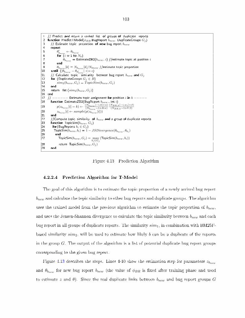
103

1 // Predict and return a ranked list of groups of duplicate reports2 function PredictTModel(φBR,BugReport bnew, DuplicateGroups Gj)3 // Estimate topic proportion of new bug report bnew4 repeat5 θ′bnew

← θbnew

6 for (i = 1 to Nb)7 θbnew = EstimateZB2(bnew, i) //estimate topic at position i8 end9 θbnew [k] = Nbnew [k]/Nbnew //estimate topic proportion10 until (|θbnew − θb′new

| <= ε)

11 // Calculate topic similarity between bug report bnew and Gj12 for (DuplicateGroups Gj ∈ B)13 sim2(bnew, Gj) = TopicSim(bnew, Gj)14 end15 return list (sim2(bnew, Gj))16 end17 // −−−−−− Estimate topic assignment for position i in b −−−−−18 function EstimateZB2(BugReport bnew,, int i)

19 p(zbnew [i] = k)← (Nbnew [−i,k]+α)(Nbnew−1+Kα)

(NBR,k[−i,wi]+β)

(NBR,k−1+V β)

20 zbnew [i]← sample(p(zbnew [i]))21 end22 //Compute topic similarity of bnew and a group of duplicate reports23 function TopicSim(bnew, Gj)24 for(BugReports bi ∈ Gj)25 TopicSim(bnew, bi) = 1− JSDivergence(θbnew , θbi )26 end27 TopicSim(bnew, Gj) = max

bi∈Gj

(TopicSim(bnew, bi))

28 return TopicSim(bnew, Gj)29 end

Figure 4.13 Prediction Algorithm

4.2.2.4 Prediction Algorithm for T-Model

The goal of this algorithm is to estimate the topic proportion of a newly arrived bug report

bnew and calculate the topic similarity to other bug reports and duplicate groups. The algorithm

uses the trained model from the previous algorithm to estimate the topic proportion of bnew,

and uses the Jensen-Shannon divergence to calculate the topic similarity between bnew and each

bug report in all groups of duplicate reports. The similarity sim1, in combination with BM25F-

based similarity sim2, will be used to estimate how likely b can be a duplicate of the reports

in the group G. The output of the algorithm is a list of potential duplicate bug report groups

corresponding to the given bug report.

Figure 4.13 describes the steps. Lines 4-10 show the estimation step for parameters zbnew

and θbnew for new bug report bnew (the value of φBR is �xed after training phase and used

to estimate z and θ). Since the real duplicate links between bnew and bug report groups G

104

are unknown, we use LDA Gibbs sampling equation to estimate the new bug report's topic

assignment and topic proportion (Case 1, Section 4.1). The estimation for zbnew is described in

EstimateZB2 (lines 18-21). In the equation, Nbnew [−i, k] is the number of words in bnew (except

the current position i) that are assigned to topic k. Nbnew is the total number of words in bnew.

NBR,k[−i, wi] is the number of words wi in the collection of bug reports B (except the current

position) that are assigned to topic k. NBR,k is the number of words in B assigned to k.

To �nd the topic similarity between bnew and a group of duplicate reports Gj , we calculate

TopicSim(bnew, Gj) (lines 12-14). TopicSim(bnew, Gj) (lines 23-29) is calculated by �nding the

maximum topic similarity between bnew and all bug reports bis in Gj (line 27). We use the

Jensen-Shannon divergence (JSD) to measure the distribution distance between bnew and each

bi (line 25). Since JSD is a symmetric measure in [0..1], 1 − JSD is topic similarity in [0..1].

Finally, the algorithm returns a list of topic similarity values between bnew and all groups of

duplicate reports.

4.2.2.5 Training for Combined Model DBTM

DBTM is linearly combined from T-Model and BM25F. Thus, we need to determine α1

and α2 for calculating the similarity between bug reports and duplicate report groups. Since

α1 +α2 = 1 by de�nition, topicmodel has to learn α1 only. α1 can be learned from the training

set by using simple cross-validation and a searching algorithm.

Figure 4.14 shows the training algorithm. Parameters are initialized at lowest possible values

(lines 3-4). A training set is used for k-fold cross validation, thus, at each cross validation step,

we have (k−1) folds of training duplicate report groups Gtrain and one remaining fold of testing

group Gtest. topicmodel �rst trains T-Model and BM25F model (lines 6-7). The parameters of

trained models are used for estimating text similarity levels (line 9) and topic similarity levels

(line 10) of a test bug report and a duplicate report group. Those similarity levels are combined

into sim(Btest, Gtest) via a varying weight α1 (line 15) with the step of 0.01. The combined

similarity values are used to rank the links between bug reports and duplicate report groups (line

16). Those ranked lists of links Lpred are used to evaluate a goal function MAP(Gtest, Lpred),

which is used to �nd the optimized value of α1. The α1 value corresponding to the highest

105

1 // −−−−−−−−−− Training ensemble weight α1 −−−−−−−−2 function TrainAlpha(Reports B, TrainGrps Gtrain, TestGrps Gtest)3 MAP (Gtest, Lpred)← 04 α1 = 05 // Training for T−Model and BM25F models6 TrainBM25F(B, Gtrain)7 TrainTModel(B, Gtrain)8 // Compute text and topic similarity of a test report and a group9 list (sim1(Btest, Gtest) = PredictBM25F(Btest, Gtest)10 list (sim2(Btest, Gtest) = PredictTModel(φBR, Btest, Gtest)11 //Estimate α1

12 for α1 from 0 to 113 increase α1 by 0.0114 // Estimate combined similarity , build a ranked list of groups15 sim(Btest, Gtest) = α1 ∗ sim1(Btest, Gtest) + (1− α1) ∗ sim2(Btest, Gtest)16 Lpred = rankedList(sim(Btest, G))17 return the α1 value corresponding to the maximum MAP18 end

Figure 4.14 Ensemble Weight Training Algorithm

value for MAP will be returned. The goal function MAP in our algorithm is the mean average

precision as proposed in [222].

MAP (Ltest, Lpred) =1

|Ltest|

|Ltest|∑i=1

1

indexi(4.7)

where Ltest is the real duplicate links in the testing set; Lpred is the ranked list of predicted

links; indexi is the index where the true duplicate group is retrieved for the i-th query. Since

MAP measures how well the algorithm ranks the true links, it can be used as a goal function

in training topicmodel.

The weights α1 and α2 trained from TrainAlpha are used to calculate the combination of

text and topic similarity sim = α1 ∗ sim1 + α2 ∗ sim2, where sim1 and sim2 are the text and

topic similarity between a bug report bnew and the duplicate report group G. The higher the

combined similarity, the more likely bnew is a duplicate of the reports in G.

4.2.2.6 Evaluation

This section describes our empirical evaluation on DBTM's detection accuracy in comparison

with the state-of-the-art approaches, REP [222] and RTM [203]. All experiments were carried

out on a computer with CPU AMD Phenom II X4 965 3.0 GHz, 8GB RAM, and Windows 7.

106

Table 4.3 Statistics of All Bug Report Data

Project Time period Report Dup Train TestOpenO�ce 01/01/2008 - 12/21/2010 31,138 3,371 200 3,171Mozilla 01/01/2010 - 12/31/2010 75,653 6,925 200 6,725Eclipse 01/01/2008 - 12/31/2008 45,234 3,080 200 2,880

Data Sets and Feature Extraction

We used the same data sets of bug reports in the open-source projects as in REP [222]

(Table 4.3). Column Time period displays the time period of collected bug reports. Columns

Report and Dup show the numbers of bug reports and duplicate ones, respectively. Columns

Train and Test show the number of the duplicate bug reports used for training and testing,

respectively. The duplication information among bug reports is also available in that data set.

The data is used to train T-Model and ensemble weights, and then used to evaluate DBTM's

accuracy in detecting the duplication between a bug report and the duplicate bug report groups.

The summary and description of a bug report were merged and considered as a document.

It then went through pre-processing such as stemming, and removing grammatical and stop

words, and single-occurrence words as in REP [222]. Then, all the words were collected and

indexed into a vocabulary. After this phase, a bug report is represented as a vector of the

indexes of its words in the vocabulary.

Evaluation Setting and Metrics

The evaluation setting is the same as in REP [222]. All bug reports were sorted in the

chronological order. We divided the data set into two sets. The training set includes the �rst

M reports in the repository, of which 200 reports are duplicates. It was used to train the

parameters for T-Model, BM25F, and DBTM. The remaining reports were used for testing. At

each execution, we ran DBTM through the testing reports in the chronological order. When it

determines a duplicate report b, it returns the list of top-k potential duplicate report groups. If

a true duplicate report group G is found in the top-k list, we count it as a hit. We then added

b to that group for later training. The top-k accuracy (i.e. recall rate) is measured by the ratio

of the number of hits over the total number of considered bug reports.

107

Figure 4.15 Accuracy with Varied Numbers of Topics

Sensitivity Analysis

In the �rst experiment, we evaluated the sensitivity of DBTM's accuracy with respect to

di�erent numbers of topics K. We ran DBTM on Eclipse data set as K was varied from 20

to 400 with the step of 20, and then measured top-10 detection accuracy. Figure 4.15 shows

the result. The shapes of the graphs for three systems are consistent. That is, as K is small

(K<60), accuracy is low. This is reasonable because the number of features for bug reports

is too small to distinguish their technical functions, thus, there are many documents classi�ed

into the same topic group even though they contain other technical topics. When the number

of topics increases, accuracy increases as well and becomes stable at some ranges. The stable

ranges are slightly di�erent for di�erent projects, however, they are large: K=[140-320] for

Eclipse, K=[120-300] for OpenO�ce, and K=[100-240] for Mozilla. This suggests that in any

value of K in this range for each project gives high, stable accuracy. The reason might be

because the number of topics in these ranges re�ect well the numbers of technical issues in

those bug reports. However, as K is larger (K>380), accuracy starts decreasing because the

nuanced topics appear and topics may begin to overlap semantically with each other. It causes

a document to have many topics with similar proportions. This over�tting problem degrades

accuracy.

Accuracy Comparison

In this experiment, we aimed to evaluate how topic-based features in our topic model T-

Model, in combination with BM25F, can help to detect duplicate bug reports. We also compared

108

Figure 4.16 Accuracy Comparison in Eclipse

our combined model DBTM with REP [222]. The parameter K of DBTM in this experiment

was selected after �ne-tuning for best results as in the previous experiment.

Figure 4.16 displays the accuracy result of DBTM in comparison with REP on Eclipse data

set. We used REP's result from [222] because the same data sets and experiment setting were

used in this study. As shown, DBTM achieves very high accuracy in detecting bug reports. For

a new bug report, in 57% of the detection cases, DBTM can correctly detect the duplication

(if any) with just a single recommended bug report (i.e. the master report of the suggested

group). Within a list of top-5 resulting bug reports, it correctly detects the duplication of a

given report in 76% of the cases. With a list of 10 reports, it can correctly detect in 82% of the

cases. In comparison, DBTM achieves higher accuracy from 10%-13% for the resulting lists of

top 1-10 bug reports. That is, it can relatively improve REP by up to 20% in accuracy.

We also compared the performance of two individual components in DBTM. We imple-

mented BM25F for comparison. As seen, the IR approach BM25F generally achieves higher

accuracy than T-Model alone (except for top-5 accuracy and above for Eclipse). Examining

this case, we see that topic model tends to group the bug reports with the same topics, but

not necessarily duplicates of one another. REP [222], an extension from BM25F, outperformed

both topic model and BM25F. Those features such as non-textual �elds (e.g. product, compo-

nent, and version) clearly help improve the performance of BM25F. However, because DBTM

achieves 10%-13% higher than REP, the topic-based features from T-Model help improve fur-

ther the performance of BM25F than those non-textual �elds. We found that in several cases,

109

Figure 4.17 Accuracy Comparison in OpenO�ce

REP was not able to detect the duplications of bug reports whose texts are not similar, while

they can be identi�ed by DBTM via topic features. That is, DBTM takes the best of both

worlds: topic modeling and information retrieval.

The results are also consistent in other data sets: OpenO�ce and Mozilla. Figures 4.17

and 4.18 display the accuracy results on OpenO�ce and Mozilla data sets, respectively. DBTM

consistently achieves very high levels of accuracy (42-43% for top-1, 65-67% for top-5, and 73-

74% for top-10 accuracy). In comparison with REP [222], DBTM consistently improves over

REP with higher accuracy from 4%-6.5% for OpenO�ce and 5%-7% for Mozilla (i.e. 10-12%

relatively).

To compare DBTM with a state-of-the-art topic model, RTM [203], we implemented the

combined model of RTM and BM25F. RTM is a topic model extended from LDA by modeling

the presence of the observed links between documents. As seen in Figures 9-11, our DBTM

outperformed RTM+BM25F from 4-7% (i.e. 5-11% relatively). This result shows that combining

topic modeling with IR can achieve better results than individual techniques. Moreover, our T-

Model is more specialized toward duplicate bug reports and performed better than RTM. This

is reasonable. First, in RTM [203], the presence of a link between two documents depends on

the similarity of their respective topic proportions. Two duplicate bug reports do not necessarily

have similar topic proportions (Section 2). They might contain more of their own topics. Second,

in practice, there are often more than two duplicate reports in a group. RTM must be trained

110

Figure 4.18 Accuracy Comparison in Mozilla

Figure 4.19 Time E�ciency

for each pair of those duplicate reports and it aims to �nd the common topic structure among

the document pair, rather than the shared buggy topic(s) among all duplicate reports in a group.

DBTM can naturally �nd the shared topic(s) and does not focus on individual pairs. For these

data sets, we found that there are many groups with two duplicate reports. Thus, the results

for RTM might get worse in other subject systems if groups contain more than two reports.

Time Efficiency

Figure 4.19 shows DBTM's time e�ciency result. The size of a project is the total of the

number of bug reports and the number of duplicate bug report groups in each data set because

training/predicting considers both bug reports and duplicate bug report groups. The sizes are

34,509, 48,314, and 82,578 for OpenO�ce, Eclipse, and Mozilla respectively. The total training

and predicting time for those projects are 1,174.8s, 1,819s, and 3,323.7s respectively. As seen,

111

the time is about linear to a project's size, e.g. time(Eclipse)size(Eclipse) ≈

time(Mozilla)size(Mozilla) . Importantly, DBTM

is highly e�cient. For a large project like Mozilla, it took about 5 minutes for training (which

could be run in background). For predicting, on average, prediction time for one bug report

are just 0.031s, 0.035s, and 0.041s for OpenO�ce, Eclipse, and Mozilla, respectively. In brief,

DBTM is scalable and e�cient to be used interactively in detecting duplicate bug reports.

Interesting Case Studies Figure 4.20 shows two duplicate bug reports detected by DBTM.

Except the terms NPE (NullPointerException) and StructuredViewer, which are popular and

common in the project, the two reports contain several di�erent terms because the reporters

found the bug in two di�erent usage scenarios. That leads to di�erent exception traces: one

involving image updating, and another on widget selection. We noticed that when running

BM25F model by itself, bug report #225169 is ranked 8th in the list that could be duplicate

of bug report #225337 due to the dissimilarity in texts. However, after extracting topics via

the co-occurrences of other terms such as startup, �rst time, RSE perspective, wizard, etc in the

previous duplicate reports (e.g. from bug report #218304, not shown), DBTM ranked it at the

highest position and detected them as duplicate ones.

Threats to Validity We evaluated only on three open-source projects. Di�erent projects might

have di�erent quality of bug reports. However, Eclipse, Mozilla and OpenO�ce are long-lasting

projects and were used in prior research. They are su�ciently representative for our comparison.

We also should validate our method on commercial projects.

112

Bug Report #225169

Summary: Get NPE when startup RSE on a new workspace

Description:

Using Eclipse M5 driver and RSE I20080401-0935 build. Start eclipse on a new workspace, and switch to RSE perspective.

I could see the following error in the log. But otherwise, things are normal.

java.lang.NullPointerException at

org.eclipse.....getImageDescriptor(SystemView...java:123)

...

at org.eclipse....doUpdateItem(AbstractTreeViewer.java:1010)

at org.eclipse....doUpdateItem(SafeTreeViewer.java:79)

at org.eclipse....run(StructuredViewer.java:466)...

������������������������

Bug Report #225337

Summary: NPE when selecting linux connection in wizard for the �rst time

Description:

After starting an eclipse for the �rst time, when I went select Linux in the new connection wizard, I hit this exception.

When I tried again a few times later, I wasn't able to hit it.

java.lang.NullPointerException at

org.eclipse....getAdditionalWizardPages(RSEDefault...:404)

...

at org.eclipse....updateSelection(StructuredViewer.java:2062)

at org.eclipse....handleSelect(StructuredViewer.java:1138)

at org.eclipse....widgetSelected(StructuredViewer.java:1168)...

Figure 4.20 Duplicate Bug Reports in Eclipse

113

CHAPTER 5. APPLICATIONS: SOURCE CODE AND API

RECOMMENDATION

5.1 DNN4C: Code Recommendation using Deep Neural Network-based

model

5.1.1 DNN Language Model for Code

5.1.1.1 Overview and Key Ideas

In this work, we develop Dnn4C, a DNN-based LM for source code, that complements

the local history of n-gram by additionally incorporating syntactic and semantic contexts. We

adapted Huang et al. [88]'s model for our new code features listed in Section 3:

1. Syntaxeme and sememe sequences as contexts. While existing deep learning LMs

use only lexical code tokens with limited contexts, we also attempt to parse the current �le

and derive the syntaxeme and sememe sequences for those tokens (if possible), and use those

sequences as contexts. We expect that with information on the current syntactic unit and

data/token types, Dnn4C is able to capture patterns at higher abstraction levels, thus, leading

to more correct suggestion. For example, in Figure 5.1, with the token hasNext and the sememe

CALL [Scanner, hasNext, 0, boolean] being in the contexts, Dnn4C could rank the token next of

Scanner higher since hasNext of a Scanner object is often followed by a call to next.

2. Multiple-prototype model (DNNs). Instead of using only one DNN for all sequences

at three levels, we input each lexeme and its syntax and semantic contexts into two additional

DNNs (Figure 5.1), each of which is dedicated to incorporate one type of context. When word

meaning is still ambiguous given local context, we expect that information in other contexts can

help disambiguation [88]. As shown in Huang et al. [88], using a single DNN would not capture

114

Score(lex=”next”)

Scorelex Scoresyn Scoresem

Hidden layers

0..0010 1..0000 0..0100 000..10 …… …… …… 0010..0 …… …… ……

while ( iter hasNext next WHILE OP EXP EXP Keyword Var[Iterator,..]Call[Scaner, hasNext,

0, boolean]Var[Iterator,..]

n-1 previous lexemes

+

n-1 previous syntaxemes n-1 previous sememes

iter

0..0100

DNNlex DNNsyn DNNsem

Figure 5.1 Context-aware DNN-based Model: Incorporating Syntactic and Semantic Contexts

well di�erent meanings of a word in di�erent contexts as the model is in�uenced by all of its

meanings. They empirically showed that using multiple DNNs for multiple representations in

di�erent contexts capture well di�erent senses and usages of a word.

3. Training objectives. There are following objectives in training for Dnn4C: 1) to train

the �rst DNN to learn to determine the potential next code token based on the n-1 previous

lexemes, and 2) to train the two additional DNNs for contexts to discriminate each correct

next token c from other tokens in the vocabulary given the window of n-1 previous lexemes

and the syntactic/semantic contexts of that token c. That is, the score should be large for

the actual next token, compared to the score for other tokens. Speci�cally, let us have the

current sequence lex of n-1 prior lexemes. We aim to train Dnn4C to discriminate the actual

next token c (appearing after lex) from the other tokens in the vocabulary. Let Scoresyn and

Scoresem be the scoring functions for two DNNs modeling syntactic and semantic contexts.

We aim that with the input lex, they give the scores Scoresyn(c, syn) and Scoresem(c, sem)

for the correct token c much higher than the scores Scoresyn(c′, syn) and Scoresem(c′, sem) for

any other token c′ in the vocabulary. syn and sem are the sequences of n-1 prior syntaxemes

and n-1 prior sememes representing the contexts for c and lex. In general, one can use any

subsequences of the syntaxeme and sememe sequences for the tokens from the beginning of a

�le to c as contexts. However, performance will be an issue when the lengths of those sequences

are large. Thus, we used the same length (n-1) for syntaxeme and sememe sequences.

As an example, we want to have the scores Scoresyn and Scoresem for the token next of

Scanner to be higher than the scores for other tokens. Mathematically, as suggested in [88, 43],

115

0

0

010

00

01

0

10

00

0

lex1

lex2

lexn-1

Lexical level

Projection

Syntactic levelsyn1

synn-1

syn2

Semantic levelsem1

semn-1

sem2

lexn

Sco

relex

Sco

resyn

Sco

resem

+ score(lexn=wi)

———————

∑score(lexn=wi)

Syntactic-and-semantic-

context-aware DNN

wi

Figure 5.2 Dnn4C: Deep Neural Network Language Model for Code

we use the following training objective O(c, syn) that minimizes the ranking loss for each pair

of token c and sequence syn in a �le, and gives the margin of 1 between two such scores. For

the sequence lex ending with c:

O(c, syn) =∑c′∈V

max(0, 1− (Scoresyn(c, syn)− Scoresyn(c′, syn))) (5.1)

If the margin between the two scores for c and c′ is greater than 1, the max function returns 0,

helping the objective O reach its minimum. If the margin is smaller than 1, the 2nd argument

in the max function is greater than 0. Thus, by using the max function, we aim to minimize

that ranking loss for (c, syn). The same training objectives O(c, lex) and O(c, sem) are used

for lexeme and sememe sequences. Note: the projection layer could be used in each DNN (not

shown).

5.1.1.2 Model Architecture and Details

Figure 5.2 shows Dnn4C's architecture. It takes as input 3 di�erent input levels of lexemes,

syntaxemes, and sememes to predict the next lexeme. For training, for each sequence s of

length n, the correct lexeme c at the nth position of s is fed into the input lexn, which is

also fed into 3 DNNs for 3 levels (Figure 5.1). Three sequences of length n-1 for lexemes,

116

syntaxemes, and sememes corresponding to s are fed into the other inputs. For predicting, each

candidate c in the lexeme vocabulary is fed into the input lexn and Score(c) is computed and

normalized (representing how likely c is the next token of the input sequence lex1, ..., lexn−1).

All candidates c are ranked based on their scores. Details on training/predicting are given later.

Lexical level. The input at this level is the concatenated discrete feature vectors of n-1 prior

lexemes lex1, ..., lexn−1 of the current lexn. Each lexeme is represented by a vector where only

the index of that lexeme is one. The role of projection for lexemes is for word embedding, i.e.,

to map each lexeme to a continuous feature space:

h1(y) = tanh

|V |∑x=1

wp(x, y)i(x) + bp(y)

,∀y = 1, · · · ,M1 (5.2)

i(x) is the value of node x at the input; h1(y) is the output value of node y in this projection

layer; wp(x, y) is the weight of the connection from input x to output y, and bp(y) is a bias

value for node y; M1 is the number of outputs of this layer; and V is the vocabulary.

Then, the output feature vectors of this layer for n-1 prior lexemes are concatenated with

lexn: h1 = [h1(1); ...;h1(M1); lexn]. To compute the score of a node y at the lexical level, we

have:

lex(y) = tanh

(n∑x=1

wlex(x, y)h1(x) + blex(y)

),∀y = 1, · · · ,Mlex

Scorelex =Mlex∑y=1

w′lex(y)lex(y) + b′lex

(5.3)

where wlex and w′lex are the weights at the lexical level. blex(y) and b′lex are the bias values

for node y at this level.

Syntactic level. For the score from the DNN for syntactic context, we use the sequence of n-1

prior syntaxemes syn1, ..., synn−1 as context, assuming that synn is the syntaxeme for lexn. A

lexeme corresponds to only one syntaxeme, but a syntaxeme can have multiple lexemes. Each

syntaxeme is represented by a vector where only the index of that syntaxeme in the vocabulary

is set to 1, while all others are 0s. To form the syntactic context, we concatenate the vectors of

n-1 syntaxemes with the vector of the lexical token lexn right after the current lexical sequence

lex1, lex2, ..., lexn−1. Thus, we have the combined vector synh = [syn1, syn2, ..., synn−1, lexn].

117

To compute the score for a node y at the syntactic level, we use:

syn(y) = tanh

(n∑x=1

wsyn(x, y)synh(x) + bsyn(y)

), ∀y = 1, · · · ,Msyn

Scoresyn =Msyn∑y=1

w′syn(y)syn(y) + b′syn

(5.4)

where wsyn and w′syn are the weights at the syntactic level. bsyn(y) and b′syn are the bias

values for a node y at this level.

During training, several combined vectors will be formed by replacing lexn with several

other words in the lexical vocabulary. The training objective is to minimize O(lexn, syn),

i.e., the ranking loss for each pair of token lexn and sequence syn (Section 5.1.1.1). Note

that, in formula (1), Scoresyn(c, syn) is equal to Scoresyn in formula (3) where c = lexn and

syn = [syn1, ..., synn−1].

Semantic level. To compute the score from the DNN for semantic context, we perform a

similar process as the one at the syntactic level, except that the syntaxemes are replaced by the

sememes of the current lexical sequence. That is, from the combined vector for the semantic

context, semh = [sem1, sem2, ..., semn−1, lexn], we compute sem(y) and Scoresem as in (3).

The number of hidden nodes is Msem. The weights will be learned via training as well.

Similarly, the training objective is to minimize the ranking loss O(lexn, sem) for each pair

of token lexn and sequence sem.

Final score. The �nal score for each lexical token wi is the normalized one of the sum of all

three scores over all possible wi in V .

Training. We �rst parse each �le in the training corpus to produce lexeme, syntaxeme, and se-

meme sequences. We collect all sequences of lexemes with a �xed length n: [lex1, lex2, ..., lexn].

The corresponding syntaxeme synn−1 and sememe semn−1 of lexn−1 are identi�ed. We then col-

lect n-1 prior units of lexemes lex = [lex1, lex2, ..., lexn−1], syntaxemes syn = [syn1, syn2, ..., synn−1]

and sememes sem = [sem1, sem2, ..., semn−1], and use them as input to Dnn4C in Figure 5.2.

The token lexn is used as the correct next token and fed into the input labeled lexn. The score

for that token is computed with the current weights (weights are initialized in the beginning).

Then, Dnn4C randomly selects a lexical token c′ (di�erent from lexn) as a negative example for

the pair (lexn, lex), and feeds it into the input labeled lexn (instead of using the correct token

118

lexn). The score Score(c′, lex) is computed. The di�erence of the scores Score(lexn, lex) and

Score(c′, lex) is recorded. Then, the weights are updated for DNNlex to minimize the value of

the objective O(lexn, lex) (Section 4.1) by taking a gradient step with respect to this choice

c′. That is, we take the derivative of the ranking loss with respect to the weights of the DNN

as in training for Huang's model [88]. Dnn4C repeats the process for other token c′′ in the

lexeme vocabulary until reaching a certain number of iterations. As suggested in [88], when

there is su�ciently large number of iterations, the quality is as good as using stochastic gradient

descent. The training process continues in the same way to train the weights for the two other

DNNs for syntaxemes and sememes except that we use Score(lexn, syn) and Score(lexn, sem).

Details on this type of objective of minimizing ranking loss can be found in [43].

Prediction. At a point L of suggestion in a program, we process the code using PPA [45] to

construct the sequences of syntaxemes and sememes up to L. For a �xed value of n, we collect

n-1 prior lexemes, syntaxemes, and sememes (from the last token before L) and use them as

the input of Dnn4C. Then, each token c in the vocabulary V will be fed into the input labeled

lexn in Figure 3.9. The score for c is computed/normalized to show how likely the next token

is c.

5.1.2 Empirical Evaluation

In our study, we aim 1) to evaluate Dnn4C's accuracy in next-token suggestion; 2) to study

the impacts on accuracy of di�erent parameters of the model and those of syntactic and semantic

contexts; and 3) to compare Dnn4C to the state-of-the-art LM approaches.

5.1.2.1 Data Collection

To have the codebase for training, we collected several open-source Java projects from

SourceForge that have long histories and are popularly used. For comparison, we selected the

projects that were used in the state-of-the-art LM approaches (e.g., Hindle et al. [82], SLAMC

[174]). Table 5.1 shows the statistics of our dataset. It consists of 10 projects having more than

11,642 �les, with 1.15M SLOCs and 8,987K n-grams with n=4. The last 3 columns show the

sizes of the vocabularies of lexemes, syntaxemes, and sememes.

119

Table 5.1 Subject Projects

Project Rev Files KSLOCs n-grams Vlex Vsyn Vsemant 1.9.4 1,233 112.4 830,152 15,899 78 1,260antlr 3.5.1 276 40.3 264,640 5,534 77 538batik 1.7 1,447 152.8 1,174,800 21,709 76 1,590cassandra 2.1.2 960 190.9 1,450,201 18,601 78 1,330db4o 7.2 1,722 83.6 620,229 10,381 75 1,249itext 5.3.5 503 69.3 612,571 11,648 77 1,158jgit 2.3.0 1,011 101.8 858,799 13,494 78 1,295lucene 2.4.0 958 102.6 815,002 10,823 78 1,341maven 3.2.5 905 63.9 434,538 7,571 77 1,095poi 3.8 2627 231.0 1,926,035 34,747 78 2,164

5.1.2.2 Experimental Setting and Metric

We use 10-fold cross validation on each project. Source �les in a project are divided into

10 folds with similar LOCs. One fold is used for testing and the others are used for training.

To study the impacts of features in a model, we integrated the combinations of features and

performed training and testing for each newly built model.

Training. For each source �le, we use Eclipse for parsing and semantic analysis. Syntaxeme

sequences are constructed according to the procedure in Table 6.8. The sememe sequences are

built from the result returned by Eclipse. If some tokens are unparseable or semantic information

is not available, the lexical tokens are kept and annotated with the special syntaxeme and

sememe LEX. Then, the unique tokens are collected into vocabularies at the three levels. For

a pre-de�ned value of n, we collect n-grams of lexemes, syntaxemes, and sememes. For each

lexical token lexi in an n-gram, we build its index vector where only the index of that token is

set to 1. All the vectors for lexis are concatenated. Similarly, we build the index vectors for

the syntaxeme and sememe sequences. Finally, the concatenated vectors are used for training.

Prediction. For a source �le in the testing set, our evaluation tool traverses the sequence of its

code sequentially. At the position of the ith token, the language model under investigation is

used to compute the top k most likely code tokens c1, c2, ..., ck for that position, considering the

prior n-1 code tokens. Since the previous tokens might not be complete, we used PPA tool [45]

to perform partial parsing to produce the AST, and semantic analysis for the code sequence

s from the starting of the �le to the current position. From the AST and type information

120

Figure 5.3 Top-k Accuracy with Varied Numbers of Hidden Nodes

returned from PPA, we build the sequences of syntaxemes and sememes (Section 6.2.2). The

remaining unparseable code tokens are handled as special ones.

We then used the suggestion engine corresponding to the language model under investigation

to suggest the next token. If the actual token si at position i is among k suggested tokens, we

count the case as a hit. The top-k suggestion accuracy for a code sequence is the ratio of the

total hits over the total number of suggestions. Total accuracy for a project is computed on all

the positions in its source �les for the entire cross-validation process.

5.1.3 Impacts of Factors on Accuracy

In this experiment, we evaluate the impact of di�erent factors and parameters of Dnn4C on

its next-token suggestion accuracy. We chose Db4o, one of the largest subject systems for this

study.

5.1.3.1 Accuracy when Varying Size of Hidden Layer

As illustrated in Figure 3.8, Dnn4C uses the hidden layer with three DNNs in which one

DNN is for the lexical context and the other two are used to incorporate the syntax and semantic

contexts for each lexeme in a sequence. Because our design choice is to take the same length

(n-1) of the windows of sequences at all three levels as the contexts, we also set the numbers

of hidden nodes in those DNNs for those levels as equal (M = Mlex = Msyn = Msem). That

121

Table 5.2 Accuracy With Di�erent Sizes of Contexts

n Top-1 Top-2 Top-3 Top-4 Top-5 Top-10 Top-202 31.0% 44.8% 54.3% 59.2% 63.4% 77.2% 83.5%3 46.1% 61.2% 68.4% 73.5% 76.4% 83.3% 85.6%4 49.2% 62.3% 70.0% 74.5% 77.6% 83.4% 85.6%5 49.1% 62.2% 69.9% 74.4% 77.4% 83.3% 85.6%6 49.1% 62.1% 69.8% 74.2% 77.4% 83.3% 85.6%

number represents the dimensions of the new continuous-valued spaces. We set n=4, varied M ,

and measured accuracy.

Figure 5.3 shows the result. As seen, the top-k accuracy with larger k's (k=10 or 20) does

not change much when the number of hidden nodes M increases. That is, the result is quite

stable and not a�ected much by M . The shape for the graphs of the top-k accuracy values

with smaller k from 1�5 has the same trend. With smaller k values (1�5), as M is small

(M<200), accuracy is lower. This is reasonable because the number of dimensions in the new

space might be too small to distinguish a large number of inputs representing the input entities

(i.e., lexemes, syntaxemes, and sememes) and a large number of sequences. As M increases,

accuracy gradually increases. When M is larger than or equal to 900, accuracy is more stable.

This suggests that around that number, we could get high, stable accuracy. The number of

dimensions in these ranges now might provide su�ciently �ne granularity to distinguish the

inputs for this project. Such ranges are slightly di�erent among top-ranked accuracy. We

used M=900 for other experiments to save running time without sacri�cing much accuracy.

Over�tting will occur when M is large in comparison to the number of inputs [50].

5.1.3.2 Accuracy with Di�erent Sizes of Contexts

We conducted another experiment to study the impact of the size n of the contexts on

Dnn4C's accuracy. Table 5.2 shows accuracy results for di�erent values of n. As seen, when in-

creasing the size of the context window (for all three levels of lexemes, syntaxemes, and sememes)

from 2 to 4, the accuracy increases since more contexts are captured for suggestion (especially,

accuracy increases much for n from 2 to 3). However, when n ≥ 4, the accuracy is stable. When

n ≥ 7, the number of sequences is extremely large for DNN, causing scalability problem. This

122

Table 5.3 Accuracy With Di�erent Contexts

Top-1 Top-2 Top-3 Top-4 Top-5 Top-10 Top-20Lex 39.3% 53.4% 63.0% 67.2% 70.2% 77.2% 80.0%Lex+Syn 45.8% 59.7% 68.0% 72.0% 75.4% 82.5% 85.1%Lex+Sem 46.3% 61.5% 68.5% 72.5% 76.4% 82.6% 85.3%Lex+Syn+Sem 49.2% 62.3% 70.0% 74.5% 77.6% 83.4% 86.6%

result is consistent with the �nding in n-gram for texts in NLP in which n-grams for n=3-5 give

better performance [105]. This suggests me to use n=4 in other experiments.

5.1.3.3 Accuracy Without and With Di�erent Contexts

In our third experiment, we varied di�erent components for the contexts in our model and

measured accuracy of newly con�gured models. Table 5.3 shows the result. The �rst row is for

Dnn4C con�gured with only lexemes. This also corresponds to the DNN LM model in [16], but

operates on lexemes. The second row is for the model with both lexemes and syntaxemes. The

third row is for the one with both lexemes and sememes. The last row corresponds to Dnn4C

model with all three types of features.

As seen, the models with contexts achieve better accuracy than the DNN LM that treats

source code as textual tokens and does not consider the syntactic and semantic contexts. With

the addition of only syntaxemes, the relative improvement in top-1 accuracy (i.e., with a single

suggestion) is 16.5%. Examining the cases, we can see that with the syntaxemes as syntactic

context, the lexical tokens relevant to surrounding ones are ranked higher because the grammar

rules have restricted the valid syntactic units at a suggestion point. Concrete examples are

presented in Section 5.1.6. Combining semantic context via sememes with lexemes actually

improves better than adding syntactic context via syntaxemes to lexemes (comparing Lex+Sem

and Lex+Syn). The model Lex+Sem relatively improves 18.1% at top-1 accuracy over the

model Lex. After investigating, we found that data types and token types allow Lex+Sem to

rank the correct token at a suggestion point higher than Lex+Syn with the syntactic context

of surrounding syntactic units. For example, pairs of API calls that often go together (e.g.,

Scanner.hasNext and Scanner.next) are a good indication to suggest the second one if the �rst

123

one is encountered. In this case, Lex+Syn ranks multiple identi�ers (for method calls) higher

than other types of tokens, but Scanner.next might not be the top one.

Dnn4C with all three levels achieves even higher accuracy (last row). In comparison to the

state-of-the-art DNN LM (operating on lexemes), Dnn4C has good relative improvement in

accuracy: 25.2% (top-1) and 10.5 (top-5). Importantly, it achieves high accuracy. In one out

of two cases, with a single suggestion, Dnn4C is able to correctly suggest the next token. In 3

out of 4 cases, the correct token is in the list of 4 suggestions from Dnn4C. With 5 suggestions,

it suggests the correct token in 78% of the time.

5.1.4 Accuracy Comparison

5.1.4.1 Comparison to n-gram, SLAMC, DNN, RNN LMs

This section presents our experiment to compare Dnn4C to the state-of-the-art approaches.

We compare it to n-gram LM used in Hindle et al. [82], Deep Neural Network LM (DNN

LM) [16], Recurrent Neural Network LM (RNN LM) [150, 235] used in White et al. [235], and

SLAMC [174], our prior work on semantic LM. Note that the original DNN LM [16] works on

texts and RNN LM [150] was applied on only lexical code tokens by White et al. [235]. However,

in the previous experiment, we have shown that adding syntaxemes and sememes improves over

using only lexemes for DNN LM. Thus, in this experiment, for DNN LM and RNN LM, we

used as input all three sequences of lexemes, syntaxemes, and sememes by concatenating their

vectors. SLAMC [174] is a LM that works on the n-grams of sememes and lexemes to predict

the next lexical token (no syntactic information is used). It explores the pairs of tokens that

often go together to improve its accuracy as well. It also integrates the topics of the current

�le via Bayesian inference into a n-gram topic model [174]. We did not compare our model to

the one by Tu et al. [227], which improves over n-gram with caching of entities' names, because

SLAMC was shown to outperform that model with caching. We did not compare Dnn4C to

Raychev et al. [193] and GraLan [165] since they operate only on API elements.

Figure 5.4 shows the comparison on Db4o project for all top-k accuracy values for k =

1�20. As seen, Dnn4C achieves higher accuracy than the other approaches. At top-1 accuracy,

124

Table 5.4 Accuracy Comparison on All Projects

Project Top n-gram SLAMC DNN LM RNN LM Dnn4Cant 1 45.7% 49.5% 51.3% 52.1% 54.3%

2 57.1% 60.3% 67.4% 64.8% 70.6%5 63.6% 65.8% 78.5% 78.4% 83.7%

antlr 1 50.0% 53.0% 54.0% 52.4% 57.4%2 61.6% 65.1% 69.0% 62.7% 70.3%5 68.7% 70.8% 81.9% 72.5% 83.5%

batik 1 55.8% 59.0% 59.4% 61.1% 64.8%2 69.3% 70.2% 74.6% 73.2% 78.5%5 73.5% 73.7% 84.3% 84.0% 88.2%

cassandra 1 44.9% 48.2% 48.7% 51.4% 54.7%2 53.7% 57.4% 63.8% 64.0% 66.7%5 61.2% 64.0% 78.9% 79.7% 80.3%

db4o 1 34.0% 38.7% 42.3% 44.1% 49.2%2 41.7% 46.6% 56.4% 57.4% 62.3%5 47.5% 50.1% 73.2% 73.1% 77.6%

itext 1 45.3% 48.7% 49.0% 51.1% 55.3%2 60.3% 64.1% 64.4% 61.4% 68.0%5 69.3% 72.1% 79.7% 70.9% 82.6%

jgit 1 46.0% 49.0% 49.0% 56.4% 53.8%2 60.9% 63.6% 64.4% 65.4% 68.0%5 70.6% 72.2% 79.6% 73.7% 82.6%

lucene 1 48.0% 52.2% 53.0% 53.4% 57.2%2 60.6% 63.5% 68.9% 69.1% 73.0%5 71.6% 73.6% 82.6% 82.9% 85.2%

maven 1 39.1% 43.4% 43.1% 44.7% 47.6%2 49.0% 52.7% 58.7% 56.5% 62.8%5 54.9% 58.4% 71.9% 67.9% 75.2%

poi 1 38.6% 42.4% 44.8% 43.9% 49.3%2 47.5% 51.4% 59.0% 52.9% 63.3%5 55.6% 57.9% 73.2% 60.5% 77.4%

Dnn4C has relative improvements of 11.6%, 16.3%, 27.1%, and 44.7% over RNN LM, DNN

LM, SLAMC, and n-gram models, respectively. At top-5 accuracy, such improvements are

6.2%, 6%, 54.9%, and 63.4%. The three NN-based models achieve higher accuracy than the

two n-gram-based ones, SLAMC and n-gram LM. Such comparison was reported for texts in

NLP [50]. This result con�rms such comparison for source code. Among the NN-based models,

with the same 3 features, Dnn4C outperforms RNN LM and DNN LM relatively 11.6% and

16.3% at top-1 accuracy. At a higher top rank k from 10�15, Dnn4C has much higher accuracy

than n-gram ( 68.9% relatively) and SLAMC ( 66.0%), and higher than both RNN and DNN

LMs.

125

Figure 5.4 Top-k Accuracy of Di�erent Approaches on Db4o

Table 5.5 Mean Reciprocal Rank (MRR) Comparison

Project N-gram SLAMC DNN LM RNN LM Dnn4Cant 0.537 0.568 0.639 0.639 0.662antlr 0.584 0.616 0.662 0.628 0.695batik 0.640 0.674 0.706 0.719 0.737cassandra 0.519 0.555 0.616 0.638 0.656db4o 0.400 0.439 0.581 0.586 0.611itext 0.577 0.617 0.625 0.601 0.656jgit 0.588 0.619 0.673 0.647 0.701lucene 0.599 0.631 0.689 0.681 0.713maven 0.463 0.524 0.558 0.553 0.578poi 0.459 0.492 0.563 0.516 0.583

Table 5.4 shows the comparison result for all projects for three top-ranked accuracy. At top-1

accuracy, Dnn4C achieves relative improvements from 14.8�44.7% over n-gram, 8.3�27.1% over

SLAMC, 5.9�16.3% over DNN LM, and 5.6�11.6% over RNN LM.

Mean Reciprocal Rank (MRR). We also measured Mean Reciprocal Rank (MRR) to evaluate

the models based on the ranked list of suggested tokens. The MRR value is computed as the av-

erage of the reciprocal ranks of results for a set of suggestion cases: MRR = 1|Ttest|

|Ttest|∑i=1

1indexi

where indexi is the index of the actual (correct) token in the resulting ranked list at the i-th

suggestion, and |Ttest| is the number of suggestion cases. The closer to 1 the MRR value, the

better the ranking of a model.

As seen in Table 5.5, Dnn4C can achieve the highest MRR of 0.737, meaning that on average

in 2 suggestion cases, it can correctly rank the actual token as the top candidate in one case

and at the second place in the resulting list in the other case. For all projects, MRR is 0.66 on

126

average. That is, among 3 cases, it would rank the actual token at the second place in two cases,

and likely rank the actual token as the top candidate in the other case.

In comparison, Dnn4C improves MRR accuracy relatively over the n-gram model up to

52.6%, over SLAMC up to 39.1%, over DNN LM up to 6.4%, and over RNN LM up to 13.0%.

Thus, for a suggestion, the actual next token is generally ranked higher in Dnn4C's resulting

list than in the resulting lists of others.

In brief, Dnn4C consistently achieves better accuracy than others.

5.1.4.2 Comparison with Bayesian-based LM

In Dnn4C, we incorporate syntactic and semantic features of the contexts by adapting

Huang's model [88] into a context-aware DNN-based one. In this experiment, we aimed to

compare that DNN-based context-incorporating method via training objective to the Bayesian

inference-based incorporating method, which was used in the existing work SLAMC [174]. In

our previous experiment, we compared Dnn4C and SLAMC. But that experiment did not

achieve our above goal since SLAMC uses only lexemes and sememes, and does not include

syntaxemes. To compare our DNN-based feature incorporating method and the Bayesian-based

one in SLAMC, we extended SLAMC into a new Bayesian-based LM (denoted by BLM), that

incorporates all three types of features (lexemes, syntaxemes, and sememes) as used in Dnn4C

but with Bayesian Inference as in SLAMC [174]. SLAMC combines the features in lexemes

and sememes using Bayesian inference-based n-gram topic model [174]. The idea is that the

probability that a token c appears is estimated based on the prior n-1 lexical tokens Lex and

their sememes Sem, as well as the topic k of the token in the current �le in which topics as

a hidden factor have the causal relations with Lex and Sem. We used the same computing

mechanism of SLAMC but incorporated the syntaxemes for the syntactic context to estimate

the probability that c appears: P (c|Lex, Syn, Sem). The computation for such probability

during training and predicting processes uses Bayesian inference with n-gram topic model in

the same way as in SLAMC [174].

Results. As seen in Table 5.6, Dnn4C relatively outperforms BLM up to 19.1% at the top-1

accuracy and up to 47.6% at the top-5 accuracy. At the higher top ranks, the gap between

127

Table 5.6 Comparison of Dnn4C and Bayesian-based LM

Model ant antlr batik cas db4o

top-1 BLM 51.3% 55.6% 61.5% 50.8% 41.0%DNN4C 54.3% 57.4% 64.8% 54.7% 49.2%

top-2 BLM 62.5% 66.4% 71.3% 59.1% 48.7%DNN4C 70.6% 70.3% 78.5% 66.7% 62.3%

top-5 BLM 67.9% 72.1% 74.8% 65.3% 52.1%DNN4C 83.7% 83.5% 88.2% 80.3% 77.6%

MRR BLM 0.580 0.628 0.686 0.566 0.450DNN4C 0.662 0.695 0.737 0.656 0.611

Model itext jgit lucene maven poi

top-1 BLM 52.5% 51.1% 54.4% 45.0% 44.3%DNN4C 55.3% 53.8% 57.2% 47.6% 49.3%

top-2 BLM 66.6% 51.1% 65.6% 54.3% 53.4%DNN4C 68.0% 53.8% 73.0% 62.8% 63.3%

top-5 BLM 73.7% 64.7% 75.5% 60.0% 59.4%DNN4C 82.6% 68.0% 85.2% 75.2% 77.4%

MRR BLM 0.629 0.630 0.642 0.533 0.503DNN4C 0.656 0.701 0.713 0.578 0.583

Dnn4C and BLM is even larger (not shown). This result shows that using the same set of features

of lexemes, syntaxemes, and sememes, the DNN-based context-incorporating method enables

Dnn4C to achieve better accuracy than the Bayesian-based LM with feature incorporating

method using Bayesian Inference via n-gram topic modeling as in SLAMC [174].

Let me compare the accuracy of BLM in Table 5.6 and that of SLAMC in Table 5.4. Note

that BLM is a new model that just adds into SLAMC a new feature type of syntaxemes for

syntactic context. Speci�cally, BLM with syntaxemes has a relative improvement over SLAMC

up to 7.8% for top-1 accuracy. The relative improvement is up to 4.0% for top-5 accuracy, and

gets larger for higher top ranks (not shown). This result shows that syntactic context via our

newly introduced feature type, syntaxemes, is really useful in improving next-token suggestion

accuracy in SLAMC.

5.1.5 Time E�ciency

Table 5.7 shows the training time for all models. All experiments were run on a computer

with Intel Xeon E5-2620 2.1GHz (con�gured with 1 thread and 32GB RAM). As expected,

128

Table 5.7 Training Time (in hours)

Model ant antlr bat cas db4o ite jgit luc mav poin-gram 0.01 0.01 0.01 0.01 0.01 0.01 0.01 0.01 0.01 0.02SLAMC 0.08 0.02 0.10 0.15 0.07 0.04 0.07 0.05 0.03 0.19DNN LM 9.8 3.1 12.9 19.7 9.9 5.1 9.2 7.2 4.6 14.9RNN LM 20.0 13.4 23.0 30.3 20.9 15.3 19.8 20.8 8.9 35.9Dnn4C 10.4 3.6 13.6 20.6 11.1 5.8 10.2 8.3 5.2 26.4

the three NN-based LMs have much higher training time than the counting-based models (n-

gram and SLAMC [174]). However, they achieve much higher accuracy as shown earlier. The

training process can be done o�-line, while each prediction in all models is less than a second,

thus, making Dnn4C suitable for interactive use in IDEs.

5.1.6 Case Studies

In addition to the illustrating examples in the introduction and motivation, we also inves-

tigated and found several other cases in which Dnn4C is able to correctly suggest a next token

due to the use of syntactic and semantic contexts. Let me take a few to explain di�erent kinds

of examples in our study.

Case 1. We found this kind of examples in which Dnn4C correctly made a suggestion in its

top-ranked list due to the use of syntactic context, while n-gram did not because the lexical

sequence was not encountered in the training data (i.e., was not captured with any n-gram).

Speci�cally, after the sequence public void testClassConstraint, Dnn4C suggests the token `(' as

the top candidate. Because public void testClassConstraint(...) is a test method and does not

occur in the training data, n-gram did not rank the token `(' in its top-20 candidates. However,

Dnn4C is able to learn the next token `(' via the syntactic context with the syntaxeme sequence

MOD VOID ID coming before `(' from other method declarations with a modi�er, a type void,

and an identi�er. That is, syntaxemes allow Dnn4C to capture the syntactic units from a code

portion and apply for prediction at another place with the same syntactic context. As another

example, the 5-gram �catch `(' Db4oException e `)'� did not appear in the training set, and n-

gram failed to rank it as the top candidates. However, Dnn4C uses syntaxemes and recognizes

129

the syntax CATCH OP NAME ID CP at other locations. Thus, it can suggest CP, i.e., the token

`)'.

Case 2: The second kind of examples is similar to the �rst except that Dnn4C uses sememes

to help suggestion. An example of this isListIterator listIter = nodes.listIterator();

while (listIter._Dnn4C can recommend the token hasNext (with rank #4), while n-gram does not have it

in the top-20 candidates. The reason is that the 5-gram �while, `(', listIter,`.', hasNext� has not

been seen in the training set. In contrast, by encoding the sequence with the sememes WHILE

OP VAR[ListIterator] PE, Dnn4C sees that sememe sequence in other places despite of di�erent

variables' names. Thus, with the type information, it can suggest CALL [ListIterator, hasNext,

0, boolean], which corresponds to the lexeme hasNext.

5.1.7 Examples on Neighboring Sequences

In NLP, researchers have shown that DNN is able to connect and project the words that are

semantically or grammatically related into nearby locations (at least along some dimensions) in

that continuous-valued feature space [50]. In this experiment, we study the examples in which

Dnn4C with its DNN machinery is able to learn the connections at a higher level of abstraction

between the sequences of lexical tokens, in order to support code suggestion.

To do that, we �rst searched for the nearest neighbors of each sequence l of length n. We

considered all possible sequences l of length n in the corpus. We put each sequence l to the

DNN for lexemes (DNNlex) of Dnn4C (Figure 3.9) (no syntaxeme and sememe is used because

we focused on DNN's abstracting capability). We then collected the vector after projection

in the continuous-valued space with M1 dimensions. Let me call the corresponding projected

vector h1(l)=[h11(l), ..., hM11 (l)]. Then, the distance between two sequences l1 and l2 of length

n is measured by the Euclidean distance between h1(l1) and h1(l2). For each sequence l, we

measured its distance to each of other sequences, and then ranked the other sequences according

to their distances in the list of nearest neighbors of l.

Table 5.8 shows some sequences of lexemes and their �rst two nearest neighbors. As seen,

neighboring sequences seem to have common syntactic and/or simple semantic roles (e.g., getter

130

Table 5.8 Examples of Nearest Neighbors of Sequences in Db4o

Sequence Neighbor 1 Neighbor 2

static void main ( static void retrieveSnapshots- static void retrieve-SequentiallyImproved ( AllPilotQBE (

new File ( new Integer ( new NotStorable (double [ ] int [ ] Object [ ]List < Pilot > Predicate < Pilot > List < SensorReadout >public double public Car getCar ( public double

getPressure ( getOilTemperature (

methods in the last row). The last two examples are the cases where n-gram model was not

able to rank the actual tokens in the top-20 list, while Dnn4C correctly suggests them as top

candidates due to the use of DNN. Those sequences were not seen in the training data, but

DNN is able to use one of their neighboring sequences for suggestion.

5.1.8 Limitations and Threats to Validity

Limitations. As other DNN-based approaches, the training time and memory requirement

in Dnn4C are high, despite the improvement over neural networks. We could explore parallel

computing infrastructures for DNNs such as CUDA GPU-Accelerated DNNs [44]. Second,

Dnn4C supports only the sequence of tokens. However, data and control dependencies in code

are not always captured well with sequences with limited sizes, thus, leading to inaccuracy. We

could explore the graph structures with DNN to address that as in GraLan [165]. Third, Dnn4C

rely on a window of history, thus, missing long and meaningful sequences. Fourth, since the

number of inputs of an DNN must be determined, we cannot support contexts with varied sizes.

Finally, there is no algorithm to learn the optimal models' parameters, thus, the tuning process

is mainly empirical.

Threats to Validity. All projects are written in Java and might not be representative. However,

our current dataset contains a very large number of SLOCs. We will explore other programming

languages in future. In our evaluation, our simulated process is not truly program editing. The

result might also be di�erent due to the use of partial program analysis tool and the DNN

infrastructure, Deeplearning4j [51] (upon which we built Dnn4C), and the RNN toolkit [198].

131

5.2 GraPacc: API Usage Recommendation using Pattern-based Model

In this section, I introduce GraPacc, a Graph-based Pattern-oriented, Context-sensitive tool

for Code Completion which is based on pattern-based model (section 3.4). It takes as an input

a database of usage patterns and completes the code under editing based on its context and

those patterns.

5.2.1 Important Concepts

De�nition 5.2.1 ( Query) A query is a code fragment under editing, i.e. a sequence of

textual tokens written in a programming language.

1 Display display = new Display();2 Shell shell = new Shell( display ) ;3 ...4 Button button = new Button(shell, SWT.PUSH);5 FormData formData = new FormData();6 button._

Figure 5.5 SWT Query Example

A query is generally incomplete (in term of the task that is intended to achieve) and might

not be parsable. Figure 5.5 illustrates a code fragment as a query. The character _ denotes the

editing cursor where a developer invokes the code completion tool during programming.

De�nition 5.2.2 ( Feature) A graph-based feature is a sequence of the textual labels of the

nodes along a path of a Groum. A token-based feature is a lexical token extracted in a query.

The size of a graph-based feature is de�ned as the number of elements in its corresponding

sequence. Thus, in a Groum, a node has a corresponding graph-based feature of size 1, and an

edge has a graph-based feature of size 2. Larger features can be built from a path in the Groum.

In Figure 5.6a, there are a size-1 graph-based feature [Shell.new], a size-2 graph-based feature

[Shell.new, Shell.pack], a size-3 graph-based feature [Shell.pack, Shell.open, Shell.isDisposed], etc.

In GraPacc, a token-based feature always has its size equal to 1 and is used to represent the

usage of a class, a method, or a control structure in the current (incomplete) code. For example,

132

Display.new

Shell.new

Shell.pack

Shell.open

Shell.isDisposed

Display.readAndDispatch

Display.sleep

Display.dispose

IF

WHILE

Display Shell

datadependency control dependency

data node

action node

control node

Button.new

Button.setText

Button.setSize

Button.setLocation

Button

Button.new

Button.setText

Button

Button.setLayoutData

FormData.new FormData

a. b.

c.

Figure 5.6 SWT Usage Patterns

the query for (Iterator _ is incomplete and can not be parsed into an AST. However, GraPacc

still extracts two tokens for and Iterator, and uses them to match this query to the patterns that

have the usages with a for loop and an Iterator variable.

To measure the similarity of any two features, GraPacc de�nes a function sim that compares

their textual similarity and the orders of their elements (see Section IV for details).

To compare a query against a pattern via features, GraPacc also takes into account the

context information of the query. Such information is modeled via the context-sensitive weights

associated with the features. That is, context-sensitive weights measure the signi�cance of the

features in a query based on the relations of the features to the focus editing position (user-based

factor) and based on the structure of the query's Groum (structure-based factor). Based on the

similarity of the features and their corresponding context-sensitive weights, GraPacc de�nes a

relevance measure fit between a query and a pattern, in order to rank the candidate patterns

to a query. The details of function fit and weights are presented next.

5.2.2 Query Processing and Feature Extraction

GraPacc analyzes the query Q (i.e. the code under editing) and extracts its context-sensitive

features and weights in four main steps: 1) tokenizing the input Q to extract lexical tokens,

133

Display.new

Shell.newDisplay Shell

Button.new Button

FormData.new FormData

focus node

Figure 5.7 Graph-based Usage Model of Query

which could be used as token-based features; 2) using Partial Program Analysis (PPA) tool [45]

to parse the input code into an AST; 3) building the corresponding Groum from the AST; and

4) extracting the graph-based features from that Groum, collecting the token-based features

from the un-parsable tokens (i.e. the tokens without associated AST node), and determining

the context-sensitive weights for the extracted features.

5.2.2.1 Tokenizing

GraPacc breaks the code Q within the current method into lexical tokens, records their loca-

tions, and computes their distances to the editing cursor. After tokenizing, GraPacc keeps the

keywords related to the control structures (e.g. while, if, for, case, etc) and object instantiation

(new). Unrelated keywords (e.g. public, class, void, etc) are not used in query formulating but

kept for later code completing.

5.2.2.2 Partial Parsing

If the current code under editing is not parsable by Eclipse's Java parser, GraPacc will use

the PPA tool [45] to handle the query. The PPA tool, as an Eclipse's plugin, accepts a portion

of code and returns an AST with all possible type binding information. However, in some cases,

there might exist some unresolved nodes, for example, their types are undeterminable in the

query. Thus, they are assigned with an UNKNOWN type.

134

5.2.2.3 Groum Building

GraPacc constructs the corresponding Groum from the AST provided by PPA in the previous

step using the constructing algorithm from our prior work [176]. Due to the incompleteness of

the query code, the unresolved nodes in the AST are discarded. They are considered as tokens

and used to extract token-based features. The data nodes corresponding to the variables of

the data types that are not resolved to fully quali�ed names are kept with only simple names.

Figure 5.7 shows the Groum built for the query example in Figure 5.5. As seen, the objects

shell, button, bData, and display are resolved to the data nodes labeled with their types Shell,

Button, FormData, and Display, respectively. Node Button is denoted as the focus node, because

the token closest to the editing cursor is button.

5.2.2.4 Feature Extracting and Weighting

In this step, GraPacc extracts the graph-based features from the Groum built for the query,

and other features for the retained tokens.

Feature Extracting. GraPacc �rst maps each node in the Groum built in the previous step

back to the tokens built in the Tokenizing step. For example, data node Button in the Groum

drawn in Figure 5.7 is mapped to three tokens of the query listed in Figure 5.5: Button (line 4),

button (line 4), and button (line 6). The �rst token denotes the type annotation of the variable

button corresponding to that data node, and the two other tokens are the two references of

that variable. After the mapping, any token that does not correspond to any node in the

Groum is selected as a token-based feature. Next, di�erent features are extracted from various

paths in the Groum. Since there might be a large number of paths, only the paths with

limited sizes (L ≤ 3) are considered. This limit were determined experimentally in our prior

work to achieve high accuracy in Groum matching [176]. Moreover, using large-size features

reduces performance signi�cantly because the number of features increases exponentially to the

maximum size of features. From now on, we use the graph-based feature and its corresponding

path interchangeably.

135

Feature Weighting. When a feature (graph-based/token-based) is extracted, its weight repre-

senting its context-sensitive signi�cance is also computed as follows:

w(q) = (ws(q) + wc(q))× wf (q) (5.5)

a. ws(q) indicates the structure-based factor of feature q via its size (from 1 to 3): ws(q) =

1 + size(q). That is, a longer feature represents more information, and is assigned with higher

weight. The rationale is that a long feature allows GraPacc to capture stricter dependencies

among several nodes in the path for that feature. The addition of 1 aims to reduce the relative

di�erence between features of di�erent sizes, e.g. if minsize=1, maxsize=3, then (3+1)/(1+1)

< 3/1, thus, making the e�ect of the size feature on the �nal weight in formula (5.5) smoother.

b. wc(q) models the structure-based factor of feature q via the centrality of the corresponding

nodes in the Groum. The rationale is that if a node has high centrality in a Groum, it plays

an important role and can be better used for matching. For example, feature Button.new is

considered to be more important than FormData.new in the query of Figure 5.7 because the

corresponding node for Button.new has more dependencies to other nodes. Thus, if feature q

has size s and the nodes of the path corresponding to q have n neighbors, wc(q) = n/s.

c. wf (q) models the user-based factor of q via its relation to the current editing position, i.e.

the focus node. For example, Button is the focus node. Thus, feature Button.new is considered

to be more important than Shell.new. wf (q) is computed based on the distance d between the

focus node and the path from which feature q is extracted: wf (q) = 1/(d + 1). d is computed

as the length of the shortest path from the focus node to a node in that path. Thus, if that

path contains the focus node, d is 0, and wf (q) is maximized. If the path contains only the

neighbors of the focus node, d is 1, and wf (q) is 0.5.

If q is a token-based feature, its size is 1, thus, its size-based weight ws is the same as

the weight of a graph-based feature of size 1. Its centrality-based weight wc is 0, because no

structural information is available. Its focus-based weight wf is 1/(d + 1), with d being its

distance to the token closest to the focus editing point in the Groum.

In the formula (1), ws(q) and wc(q) are added together while wf (q) is multiplied since ws(q)

and wc(q) represent structure-based factors (feature's size and centrality) and wf (q) is for user-

136

based factor (distance to the focus point). They are context-sensitive information in di�erent

spaces.

5.2.3 Pattern Managing, Searching and Ranking

Pattern Management. The patterns can be automatically imported from the mining results of

the pattern mining tool, GrouMiner [176], or be manually provided by the users. Each pattern

is stored as a Groum along with a textual template code fragment [176]. A parameter Pr(P ) is

stored to represent the popularity of pattern P . For the patterns mined from codebase, GraPacc

uses their occurrence frequencies in the codebase for Pr(P ). For user-provided patterns, the

user can either specify this parameter or a default value is assigned.

To support e�cient searching of patterns based on features, GraPacc uses an inverse indexing

mechanism. It extracts the graph-based features from a pattern, and for each feature p, it stores

the list L(p) of patterns from which feature p could be extracted. For each extracted feature

p, GraPacc uses a weight s(p, P ) to represent its signi�cance in each pattern P containing the

feature p. The weight s(p, P ) is computed based on the Tf-Idf weighting scheme [206]:

s(p, P ) = Np,P /NP .(logN − logNp) (5.6)

Np,P is the number of occurrences of feature p in P ,

NP is the total number of features in P ,

Np is the number of patterns containing feature p, and

N is the total number of patterns in the pattern database.

The inverse indexing list of patterns for each feature is sorted according to those weights.

Searching and Ranking. Another crucial task is to search and rank a list of relevant patterns

for the code under editing (i.e. a query). The core step is to compute the relevance degrees of

the candidate patterns to that query based on the features and context-sensitive factors/weights

computed from the query. However, there are two following challenges:

a. Due to the incompleteness of the query, there might be some extracted features that do

not exist in the pattern database (e.g. the features for the nodes whose types are unresolvable

137

to fully quali�ed names). Thus, the features in the pattern database (called pattern features)

might not exactly match to the features in the query (called query features).

b. The number of patterns in a database is often large, it is ine�cient to compute the

relevance degrees for all patterns.

For issue a, GraPacc uses the similarity function sim, which will be explained next, to �nd

the features existing in the pattern database that are best-matched to the query features. If p is

a pattern feature, q is a query feature, and sim(p, q) ≥ δ, with δ being a pre-chosen threshold,

then p is added to the set F of the mapped features for q. GraPacc uses this set to solve issue

b. For each pattern feature p ∈ F , the top-n ranked patterns in its ranked inverse indexing list

L(p) are added to the list of candidate patterns C for the relevance computation for q. After

this step, GraPacc computes the relevance measure function fit(P,Q) of each candidate pattern

P ∈ C to the query Q, ranks them based on those relevance degrees, and returns the ranked

list of patterns. Let me describe the functions sim and fit.

1) Feature Similarity sim. Function sim computes the similarity between two features.

Both graph-based features and token-based features could be considered as a sequence of label-

s/names, thus their similarity is computed mainly based on the names of those labels. GraPacc

de�nes the similarity only for two features of the same size. The similarity of two features p, q

of size k is computed as:

sim(p, q) =k∏i=1

nsim(pi, qi) (5.7)

in which nsim is the name-based similarity measure, and pi and qi are the i-th element of p

and q, respectively. The similarity degree of features with di�erent sizes is zero.

In GraPacc, a standard label pi has the following form X.Y.Z, in which X is the quali�ed

name of the package, Y and Z are the simple names of the class/method, respectively. X, Y ,

or Z might be empty. For example, for a data node, Z is empty. Sometimes, X is empty since

the package name is unresolvable in the query. Thus, for two labels X.Y.Z and X ′.Y ′.Z ′, its

name-based similarity nsim is de�ned as

α× wsim(X,X ′) + β × wsim(Y, Y ′) + γ × wsim(Z,Z ′)

α+ β + γ(5.8)

138

in which α, β, and γ are weighting parameters, and wsim is a word-based similarity value. If in a

label, two corresponding parts are missing, the corresponding term in formula (5.8) is discarded.

For example, if neither labels have the X parts, the �rst term and its weight parameter α are

discarded.

To compute the word-based similarity wsim of two strings X and X ′, GraPacc �rst breaks

them into single words using Camel convention. For example, StringBu�er is broken into two

words String and Bu�er. Then, the similarity of two labels, viewed as two sequences of words

L(x) and L(y), is de�ned as Lo/Lm, in which Lo is the length of their longest common sub-

sequence, and Lm is the average length of two sequences. This scheme enables GraPacc to

support incompletely-typed and non-exact matched entity names.

GraPacc considers a token-based feature T (size 1) as comparable to a graph-based feature

of size 1 (with some label X.Y.Z), because a token could be the name of a variable or a method

in the query and should be comparable to the label of a Groum's node of a pattern. In this

case, nsim is de�ned as

max(wsim(T,X), wsim(T, Y ), wsim(T,Z)) (5.9)

The max function is used since a token in the current code could be the name of either a

package, class, or method.

2) Pattern Matching. GraPacc models two patterns P and Q as two sets of features, each

feature has its own signi�cance weight, and each pair of features has the similarity measured

by function sim. Thus, the relevance measurement between P and Q is based on the weighted

maximum bi-partite matching, i.e. matching each feature of P to a feature of Q in order to

maximize the total similarity and signi�cance between all matched pairs of features in P and

Q. The relevance degree between a pair of features p ∈ P, q ∈ Q is computed as:

relevance(p, q) = s(p, P )× sim(p, q)× w(q) (5.10)

• s(p, P ): the signi�cance of feature p in pattern P according to the Tf-Idf scheme,

• w(q): the context-sensitive signi�cance of q in query Q,

• sim(p, q): the similarity of two features.

139

The maximal weighted match for P and Q is a map M for each feature p of P to an unique

feature q of Q such that the total weight of matched pairs

SM (P,Q) =∑

p∈P,q=M(p)

relevance(p, q) (5.11)

is maximal among all possible maps. Because GraPacc also considers the popularity Pr(P ) of a

candidate pattern, the relevance degree of the pattern P to the query Q is computed as follows:

fit(P,Q) = SM (P,Q)× Pr(P ) (5.12)

5.2.4 Pattern-Oriented Code Completion

If the user chooses a pattern P in the recommended list, GraPacc will complete the code in

the query Q according to pattern P . Generally, to do that, GraPacc �rst matches the code in

P and Q to �nd the code in P that has not appeared in Q. Then, it �lls such code into Q in

accordance with the context in Q, i.e. at the appropriate locations in Q and with the proper

names.

Let me �rst explain the general idea via an example. Let me revisit the query example in

Figure 5.7 (the corresponding code is in Figure 5.5) and assume that a user selects pattern c)

in Figure 5.6. GraPacc �rst determines that the two Button.new nodes, the two FormData.new

nodes, the two Button nodes, and the two FormData nodes in the two Groums are respectively

matched. That is, two object initializations and the assignment to the variables for Button and

FormData already existed in the query. Compared with pattern P , the nodes that have not used

include Button.setText and Button.setLayoutData. Thus, GraPacc uses the code corresponding

to those nodes to �ll in Q.

The code completing task is done via creating the corresponding sub-trees in the AST of

Q at the appropriate positions and with the proper names for the �elds and variables. For

example, to �ll in Button.setLayoutData, it �rst needs to create that method call and �nd its

position in the AST of Q (not shown). In this case, the position is next to the variable node

button in the AST of Q. Since in the pattern, Button.setLayoutData has a parameter of type

FormData (Figure 3.7c), GraPacc must �ll in that parameter with a proper name. From pattern

140

1 function GroumNodeMatching(GQ, GP )2 for each node u in GQ3 for each node v in GP4 //�nding best matching between two sets of features5 BipartiteMatching(F (u), F (v), relevance(p, q)) with p ∈ F (u), q ∈ F (v)6 match(u, v) = max(

∑{relevance(p, q)}) //matching level for (u, v)

7 //�nding the sets of best−matched nodes in P and Q8 BipartiteMatching(GQ, GP ,match(u, v))9 Return the mapping M for the nodes in GQ and GP

Figure 5.8 Groum Node Matching between Pattern P and Query Q

P , that parameter must be from the FormData node (Figure 3.7c), which is matched to FormData

in Q (Figure 5.7). It in turn corresponds to the variable formData in Q (Figure 5.5). Thus,

GraPacc chooses the name formData and �lls in line 6 of Figure 5.5. Similar process is used for

Button.setText, which is added between lines 4-5 of Figure 5.5. Therefore, the �nal result is:

1 Button button = new Button(shell, SWT.PUSH);

2 button.setText(_);

3 FormData formData = new FormData();

4 button. setLayoutData(formData);

Let me describe the algorithm in details.

5.2.5 Matching Groum Nodes in Pattern and Query

GraPacc performs code matching on Q and P on their Groums, i.e. for each node v in

P , it determines the best matched node u in Q (Figure 5.8). To do so, it retrieves two sets of

features F (u) and F (v) corresponding to the paths through u and v, respectively. It then runs a

weighted bipartite matching algorithm with the weights being measured via relevance function

(line 5). The matching degree between u and v is measured by the sum of the relevance degrees

corresponding to the best matching (line 7). After computing all matching degrees for all u and

v, GraPacc performs bipartite matching to �nd maximal aligned sets of nodes in Q and P (line

9). Then, it returns the mappingM , i.e. M(v) = u means that v ∈ P is matched to u ∈ Q, and

M(v) = null if v is not matched to any node in Q. For example, while matching the Groums for

Q in Figure 5.7 and for P in Figure 5.6c, it determines that Button.new, FormData.new, Button,

and FormData have matches. Button.setText and Button.setLayoutData are unmatched nodes.

141

1 function CodeCompletion( M , P , Q)2 //cloning AST nodes of the unmatched nodes from P to Q3 for each node v such that M(v) = null:4 T = clone(ASTP , v)5 updateName(T , M)6 pos = �ndPosition (ASTQ,T )7 updateQueryCode(T , ASTQ, pos)

Figure 5.9 Code Completion from Pattern P to Query Q

5.2.6 Completing the Query Code

After having the mapping, GraPacc performs code completing (Figure 5.9). It traverses the

un-matched nodes in the Groum of pattern P in a breadth-�rst order and for such a node, it

�nds the corresponding AST's subtree at that node in the AST of pattern P via the stored

template code of P . Then, it clones that sub-tree (line 4) and updates the name attributes

of the nodes of that sub-tree in accordance with the code in Q (line 5). After that, it �nds

the proper position for that sub-tree in the AST of Q (line 6) and attaches it to the AST via

Eclipse's AST editing support (line 7).

5.2.6.1 Finding Appropriate Names for Variables before Filling-in (updateName)

Since variables in P and Q generally are named di�erently, to be able to �ll in a variable in

P into Q, GraPacc needs to update its name accordingly. For example, although two data nodes

FormData in Figure 5.6c and Figure 5.7 are matched, the corresponding variables in ASTs are

bData and formData. To �nd such proper name, GraPacc uses the mapping M : if node v ∈ P

is matched to u ∈ Q, then the relevant name for the variable involving v will be u's name; if v

is unmatched, but is the reference/declaration of a variable corresponding to a matched node

v′ ∈ P , the relevant name for the variable involving v will be v′'s name. Otherwise, the relevant

name for v will be kept the same as in P . However, to avoid accidental duplicate names in P

with those in Q as the code is �lled in at the next step, for all nodes that are not matched and

not renamed, if they have the same names with any nodes in Q, they are renamed with new

indexes being added.

142

5.2.6.2 Finding the Position for an Unmatched Node v in P within the AST

of Q (�ndPosition)

Its position is determined via the relative position of v with respect to the matched nodes

in its neighbors in P . For example, to �nd the location to �ll Button.setText into Q, GraPacc

determines that in P , that node follows Button.new. According to the sequential order in the

code of P , it comes before FormData. With the mapping for those nodes, its location is

determined as between two AST nodes corresponding to line 4 and line 5 of Figure 5.5. The

following neighboring relations of v in a pattern are used to determine the relative positions:

• v is the initialization of a variable declaration,

• v is a parameter of a method invocation,

• v is in a conditional expression or the body of an if node,

• v is a control node/ method call having the matched nodes.

• v is a node having a sequential order with matched nodes.

If GraPacc cannot �nd the relative position for v (e.g. no matched node as a pivot), the

current focus point is used.

Note that GraPacc's code completion can be invoked on demand at any point in the cur-

rently edited code. It can search for a pattern that appears non-contiguously since it captures

control/data dependencies among the elements in an API usage backward and forward from

the invoking point. Thus, it can support both programming styles: writing line-by-line, and

creating code skeleton and then �lling in.

5.2.7 Empirical Evaluation

This section presents our experimental studies to evaluate GraPacc's accuracy in code com-

pletion. GraPacc is realized as an Eclipse plug-in. All experiments were carried out on a

machine with CPU AMD Phenom II 3.0 GHz, 8GB RAM.

143

Table 5.9 Training data for Java Utility Patterns

Project Files Methods using Java Util Mined Patterns

EclipseME 137 619 28AspectJ 1,053 5,859 155Codehaggis 20 52 4Unitmetrics 34 103 10

1 Scanner scanner = new Scanner(new File ("C:/sample.dat"));2 ArrayList<String> list = new ArrayList<String>();3 while(scanner.hasNext()) {4 list .add(scanner.next()) ;5 }6 StringBu�er strBuf = new StringBu�er() ;7 Iterator itr = list . iterator () ;8 while ( itr .hasNext())9 {10 String str = itr .next() + ":";11 strBuf .append (str) ;12 }13 System.out. println (strBuf . toString ()) ;

Figure 5.10 An Example of a Test Method

5.2.7.1 Experiment Setting

Java SDK Utility (java.util, java.io) [96] was chosen since it contains a rich set of usages

and many open-source systems have used its APIs. We collected a total of 28 open-source Java

projects using Java Utility library. We then used our pattern mining tool, GrouMiner [176], to

collect API patterns of Java Utility from a set of 4 Java projects, which were used as the tool's

knowledge (Table 5.9). Other 24 projects were used for evaluation (Table 5.10). Eventually, we

had 197 patterns in our database with 1,288 features.

We built an automatic evaluation tool and for each subject project, we �rst used it to collect

all methods using Java Utility. For such a method, we simulated a real programming situation.

We assumed that a developer partially �nished his/her coding in that method and requested

the help from GraPacc. Thus, we divided the code of the method under testing (called a test

method) into two parts: the �rst part was used as a query, and the second for evaluation.

We followed a similar automatic evaluation process for a code completion tool as in Bruch et

al. [32]. Let us explain the procedure of handling a test method via an example in Figure 5.10.

Our evaluation tool �rst collected from the test method all occurrences of the API elements

144

including method calls, object creation, data variables, and control structures that are related

to Java Utility. It sorted them in the order of their occurrences in the test method. The one

at the middle position of that sorted list was chosen as the cut point (focus point). The �rst

part of the test method from its beginning to the cut point was used as a query for evaluation.

The rationale for this way of selecting a focus point at the middle point is to avoid the cases

in which no Java Utility API element appears in the �rst part or none of them is left in the

second part of the test method. For Figure 5.10, the query is as follows:

...

StringBu�er strBuf = new StringBu�er() ;

Iterator itr =_

5.2.7.2 Evaluation Metrics

For each given query, GraPacc was invoked and it returned a ranked list of patterns. Assume

that a pattern was selected, and GraPacc would complete the code. Let me use O and R to

denote the original and the resulting code (from GraPacc) in the second half of the test method,

respectively. As explained, there might be no speci�c order between two API elements. If we

compared directly R to O based on their texts, the evaluation would be imprecise since a correct

result from GraPacc might not match exactly the writing order of API elements in O. Moreover,

the goal was to evaluate how well GraPacc completed for Java Utility elements (rather than

other elements). Thus, we compared the Groum of the resulting code R with that of the original

code O.

Let me call their respective Groums GR and GO. If a node in GR matches with a node in

GO, we count it as an correctly suggested node. If a node in GR does not occur in GO, we count

it as an incorrect node n (because a user would need to delete the corresponding code from the

recommended code). If a node in GO does not occur in GR, we consider this as a missing node

m (i.e. the user would need to manually add the corresponding code after code completion).

Note that, the original method O might use API elements that do not belong to Java Utility,

in which GraPacc has no knowledge. Thus, we counted only the missing nodes in GO relevant

to that library.

145

Accuracy is measured via precision, recall, and f-score. Precision is de�ned as the ratio

of the number of correctly recommended nodes over the total number of all recommended

nodes. Recall is the ratio of the number of correctly recommended nodes over the total number

of completion-needed nodes. We also computed f-score, a harmonic average of precision and

recall: f-score = 2 / (1/ precision + 1/recall). Higher f-score means better accuracy.

5.2.7.3 Experiment Procedure

Our evaluation tool ran GraPacc on each test method and a ranked list of patterns was

returned. To simulate a real coding situation in which a user would choose the desired pattern

(i.e. the most similar one), our evaluation tool selected the pattern with the highest f-score in

the top-5 list of the recommended patterns returned by GraPacc.

A method under test m might contain multiple Java Utility API patterns. Thus, in prac-

tice, a user might need to invoke GraPacc multiple times to get su�cient recommendations

to complete the second half of m. To simulate that, our evaluation tool iteratively invoked

GraPacc at multiple focus points in the second half of m. At each iteration, the tool selected

an additional focus point, invoked GraPacc and picked the pattern with highest f-score in the

top-5 patterns, and counted the numbers of (in)correct/missing nodes. The process continued

until all API elements in the second half were completed or no new API elements/nodes can be

correctly added (i.e. all added API elements are incorrect). This second condition simulates the

case where the user does not �nd the correct API elements returned by GraPacc and continues

coding. In each iteration, for the process to continue, at least one of API elements must be

�lled. Thus, the maximum number of iterations is equal to the number of API elements in the

second part of m.

The selection mechanism for the additional focus points with multiple iterations is based on

the variables that existed in the query O and the newly added variables via code completion.

The evaluation tool maintains a priority queue D of variables. For the �rst cut point, this

queue D was initialized with all variables in the �rst half of the test method. The variables

with shorter distances to that focus point were placed in the front of D. If a variable appears

multiple times, the distance of only its last occurrence is measured to the current focus point.

146

Table 5.10 Code Completion Accuracy Result

System Methods Patterns Variables Calls Controls Correct Incorrect Missing Precision Recall F-scoreanyedittools 81 95 151 251 74 200 22 58 90.1% 77.5% 83.3%apache-axiom 598 689 801 1,386 415 1,084 269 509 80.1% 68.0% 73.6%apache-ivy 1,400 1,923 2,121 4,291 1,620 4,480 580 1,482 88.5% 75.1% 81.3%apache-roller 1,443 1,738 1,879 3,378 1,147 3,205 536 1,501 85.7% 68.1% 75.9%Aribaweb 1,866 2,344 4,000 7,057 2,173 5,538 1,340 2,967 80.5% 65.1% 72.0%cayene 4,476 4,653 5,305 8,072 2,598 6,391 1,560 3,537 80.4% 64.4% 71.5%cvsgrapher 39 55 57 99 38 95 8 32 92.2% 74.8% 82.6%dom4j-1.6.1 565 660 764 1,324 415 1,274 107 375 92.3% 77.3% 84.1%dvsl 46 53 56 67 28 69 4 19 94.5% 78.4% 85.7%geronimo 92 114 273 398 142 356 88 128 80.2% 73.6% 76.7%jibx 843 949 1,046 1,675 514 1,412 299 569 82.5% 71.3% 76.5%Jlibrary 474 612 676 1,253 464 1,385 170 384 89.1% 78.3% 83.3%jnormalform 194 450 582 1,178 348 1,184 156 254 88.3% 82.3% 85.2%OPENWFE 1,331 1,687 1,957 4,052 1,256 3,993 598 1,139 87.0% 77.8% 82.1%PetriEditor 37 50 53 106 49 137 10 12 93.2% 91.9% 92.6%quack 36 46 67 81 32 64 13 37 83.2% 63.4% 72.0%RONEditor 366 436 446 838 350 878 144 320 85.9% 73.3% 79.1%schemaeditor 149 209 262 574 211 606 32 105 95.0% 85.2% 89.8%sdi� 506 673 943 2,609 1,123 2,405 412 1,131 85.4% 68.0% 75.7%syper 112 167 191 419 212 375 90 187 80.1% 66.7% 72.9%varia 158 256 436 949 274 854 128 298 87.0% 74.1% 80.0%VOCL 189 214 461 733 266 583 66 183 89.8% 76.1% 82.4%xaware 161 212 222 491 274 498 93 232 84.3% 68.2% 75.4%xmlrpc 26 28 29 55 35 56 9 33 86.1% 62.9% 72.7%

15,188 18,313 22,778 41,336 13,990 37,122 6,734 15,492 84.6% 71.0% 77.0%

Thus, the list D contains a variable at most once. For example, for Figure 5.10, initially, D =

[itr, strBuf, scanner, list]. GraPacc completed the code at the �rst iteration as follows:

...

StringBu�er strBuf = new StringBu�er() ;

Iterator itr = list . iterator () ;

while ( itr .hasNext()){

itr .next() ;

}

To select a new focus point, the evaluation tool considered all variables of any types in the

newly added code recommended by GraPacc. It �rst added those variables in the front of the

queue D, based on their distance to the current focus point. If a variable exists in the queue, it

will be moved to the front. Finally, the variable that was just processed will be put at the tail

of the queue. For example, the queue D was updated as follows: 1) list was moved to the front

because it was the only added element, and 2) itr was placed at the tail of D. Thus, D= [list,

strBuf, scanner, itr]. The variable at the front of D was then selected to be processed next, i.e.

the variable list. The last occurrence of that variable in the new code after completion at this

iteration was chosen to be the next focus point because its prior occurrences might not provide

147

as much context to expand a new pattern. In the example, the next focus point was at Iterator

itr = list.iterator();_.

This scheme of selecting a new focus point simulates the real situation in which a user would

focus on the variable that was most recently completed by GraPacc. This procedure is applied

to each test method. The numbers of (in)correct/missing elements are accumulated for all

test methods and iterations. Precision, recall, and f-score are computed from the accumulated

numbers for entire subject system.

5.2.7.4 Accuracy Result

We ran our evaluation tool with the above procedure. The parameters are chosen as follows:

γ=0.6, β=α=0.2, δ=0.9. They are not representative and were chosen after �ne tuning for

this experiment. Column Methods in Table 5.10 shows the number of test methods. Columns

Patterns, Variables, Calls, and Controls show the number of the recommended patterns and the

numbers of involved variables, method calls, and control nodes in those patterns, respectively.

Columns Correct, Incorrect, and Missing display the numbers of (in)correctly recommended and

missing API elements. As seen, GraPacc suggested 18,313 API patterns with 22,778 variables,

41,336 calls, and 13,990 control nodes. At each iteration, GraPacc �lled in one pattern. In

total, it �lled in 18,313 patterns for 15,188 methods (Table 5.10). Thus, it took on average 1.2

iterations to converge. It achieves very high accuracy, with up to 95% precision, 92% recall,

93% f-score. The accumulated result shows that precision, recall, and f-score values are 84.6%,

71%, and 77%, respectively. Interestingly, the average recall of 71% suggests that about 71%

of an API's usage in a project is covered by API usage patterns.

We also analyzed the incorrect and missing cases and found a few sources of inaccuracy.

First, a usage scenario requires an extra API call. This a�ects GraPacc's accuracy, however,

in practice, users can easily customize usage patterns. The second cause is due to the missing

patterns in our evaluation database. The third cause is when an API usage spans two methods

and GraPacc's suggestion is redundant.

Time E�ciency. In this experiment, we used GrouMiner [176] to mine the patterns from all 28

subject systems to collect 977 usage patterns in 7 libraries (6,378 API elements, 4,905 distinct

148

features). We ran GraPacc on the same set of 15,188 test methods (Table 5.10). The time for

each query with handling, searching, and ranking the candidate patterns, and code �lling is

about 0.7s. Thus, it is very time e�cient.

Threats to Validity. We used a simulation for users' editing actions, rather than true editing.

The focus point selection might not re�ect well users' editing. Another threat is the insu�cient

patterns mined from GrouMiner.

149

5.3 GraLan: API Usage Recommendation using Graph-based Model

In this section, I introduce GraLan, a statistical tool for Code Completion which is based

on graph-based model (section 3.6).

5.3.1 Computation based on Bayesian Statistical Inference

Let me explain how we calculate the generation probability of a new graph with Bayesian

statistical inference. We have:

Pr(C(g)|Ctxt) = Pr((g,N+, E+)|Ctxt) (5.13)

We want to compute the generation probability for the additional node and edges to g. That

probability is learned from a training set via statistical learning. To do that, we start with:

Pr(C(g)|Ctxt) = Pr(C(g)|g1, ..., gn) (5.14)

where Pr(..) represents a probability that a child graph C(g) is generated from its parent g,

and g1, ..., gn is the set of graphs including g making up the context for generating C(g).

The Bayesian model is based on the Bayes' theorem to estimate the posterior probability

given the prior probability:

Pr(A,B) = Pr(A|B)Pr(B) = Pr(B|A)Pr(A)⇒ Pr(B|A) = Pr(A|B)Pr(B)/Pr(A) (5.15)

where Pr(B|A) is the probability of a hidden variable B having a state, given the observed state

of the variable A. Pr(A|B) is the learned knowledge on the impact relation (via conditional

probability) between B and A. Pr(A) and Pr(B) are the prior probabilities that A and B have

their respective states. In GraLan, the hidden variable B represents the graph C(g) to appear

(i.e., to be generated), and the known variables As include the given graph g and the rest of the

graphs in the context Ctxt having been observed. Thus, the formula (5.14) for the generation

probability of C(g) becomes:

Pr(C(g)|g1, ..., gn) = Pr(C(g), g1, ..., gn)/Pr(g1, ..., gn)

∝ Pr(C(g), g1, ..., gn) = Pr(g1, ..., gn|C(g))Pr(C(g))(5.16)

150

1) Pr(C(g), g1, ..., gn) is the probability that all the graphs g1, ..., gn and C(g) co-appear.

2) Pr(C(g)) is the probability that the child graph C(g) appears. It can be estimated by

Pr(C(g)) = #methods(C(g))/#methods where #methods is the number of all methods in a

training dataset and #methods(C(g)) is the number of all the methods containing C(g).

3) Pr(g1, ..., gn|C(g)) is the probability that the graphs g1, .., gn appears given that C(g)

has been observed.

Similar to the n-gram model where the subsequences n-grams are assumed to be condi-

tionally independent, we assume g1,..., gn to be conditionally independent given C(g). Thus,

Pr(g1, ..., gn|C(g)) = Pr(g1|C(g))...P r(gi|C(g))...P r(gn|C(g)) (5.17)

Pr(gj |C(g))(j = 1..n) is the probability that the graph gj appears given C(g), and is

estimated by the Bayes formula:

Pr(gj |C(g)) = Pr(gj , C(g))/Pr(C(g)) = (#methods(gj , C(g))+α)/(#method(C(g))+α.#methods)

(5.18)

where #methods(gj , C(g)) is the number of all methods having both gj and C(g). A smoothing

constant α is used to avoid zero value when there is no method having both gj and C(g).

Since g belongs to the context, let g = gi. The pair g and C(g) co-appears at least in one

method, and they have parent-child relation, hence we give that pair a probability Pr(C(g)|g) =

#methods(g, C(g))/#method(g). Thus,

Pr(C(g)|Ctxt) = Pr((g,N+, E+)|Ctxt) = Pr(C(g)|g1, ..., gn)

∝ Pr(g1|C(g))...P r(gi−1|C(g))Pr(g|C(g))

Pr(gi+1|C(g))...P r(gn|C(g))Pr(C(g))

= Pr(g1|C(g))...P r(gi−1|C(g))Pr(g|C(g))Pr(C(g))..P r(gn|...)

= Pr(g1|C(g))...P r(gi−1|C(g))Pr(C(g)|g)Pr(g)...P r(gn|C(g))

= #methods(g1,C(g))+α#method(C(g))+α.#methods ...

#methods(g,C(g))#methods(g) .#methods(g)#methods ...

#methods(gn,C(g))+α#method(C(g))+α.#methods

(5.19)

The calculation of the product of probabilities, which are within [0, 1], is not resilient due

to �oating under�ow. Thus, we calculate the logarithmic values of (5.19), and use them to

151

File.new

Scanner.new

File.new

FileWriter.new

BookMetaData.new

BookMetaData.printData

Main.getMetaData

while

Scanner.close

Scanner.nextLine

1 File bookFile = new File(”books.txt”);2 Scanner bookSc = new Scanner(bookFile);34 File authorFile = new File(”authors.txt”);5 FileWriter authorFW= new FileWriter6 (authorFile); 7 BookMetaData metaData =8 getMetaData(”bookMetaData.txt”);9 metaData.printData();1011 while ( ) {12 bookSc.nextLine();13 }1415 bookSc.close();

a. b.

Figure 5.11 An API Suggestion Example and API Usage Graph

compare the additional nodes corresponding to di�erent C(gj)s.

log(Pr(C(g)|g1, ..., gn)) ∝∑j=1...n log(#methods(gj , C(g)) + α) + log(#methods(gj , C(g)))

−(n− 1)log(#method(C(g)) + α.#methods)− log(#methods(g))

(5.20)

5.3.2 GraLan in API Element Suggestion

This section explains how we use GraLan to build an engine for suggesting the next API

element for the current code. The suggestion task for API elements is to recommend an API

element upon request at a location in the current code under editing (not necessarily at the

end). An example of partially edited code is shown in Figure 5.11a. A developer requests the

engine to suggest an API call at the while loop (line 11).

5.3.2.1 Algorithm

Overview. The key idea of the API suggestion algorithm is to extract from the currently

edited code the usage subgraphs (Groums) surrounding the current location, and use them as

the context. Then, the algorithm utilizes GraLan to compute the probabilities of the children

graphs given those usage subgraphs as the context. Each child graph has a corresponding

152

1 function APISuggestion(Code C, Location L, GraphDatabase GD)2 G = BuildGroum(C)3 Ctxt = GetContextGraphs(G, L)4 NL = ∅ // a ranked list of recommended nodes5 foreach g ∈ Ctxt6 {C(g)} = GetChildrenGraphs(g, GD)7 foreach C(g) ∈ {C(g)}8 score = log(Pr(C(g)|Ctxt))9 NM = GetAddedNode(C(g))10 NL = UpdateRankedNodeList(NL, NM , score)11 return NL12 end

Figure 5.12 API Suggestion Algorithm

additional node, which is collected and ranked as a candidate of API element for suggestion.

Those probabilities are used to compute the scores for ranking the candidates.

Detailed Algorithm. Figure 5.12 shows the pseudo-code of our algorithm. The input includes

the current code C, the current location L, and the trained model with graph database GD

(see Section 5.3.2.2 for building GD). First, we use Eclipse's Java parser to create the AST for

the current code. If the incomplete code under editing is not parsable by the parser, we run the

PPA tool [45] on it. The PPA tool accepts a portion of code and returns an AST with all

available type binding information. However, in some cases, there might exist some unresolved

nodes, for example, their syntactic or data types are undetermined. Thus, they are assigned

with an unknown type. Then, we build the Groum from the AST using the Groum building

algorithm [176] (line 2). Due to the possible incompleteness of the current code, the unresolved

nodes in the AST (if any) are considered as single-node graphs. Their labels are the lexemes.

The Groum of the code in Figure 5.11a is shown in Figure 5.11b.

Next, APISuggestion determines the list of context graphs from the Groum G and the current

location L (line 3). We use the graphs that contain the APIs surrounding L as the context. One

or more of those context graphs are potentially the graphs that �generate� the child graphs in

which the corresponding additional nodes are the candidates to be �lled in at L. They represent

the usages with high impact on the selection of the API to be �lled. Details on context graphs

are in Section 5.3.2.3. Figure 5.13 shows the context graphs for the code in Figure 5.11.

Then, for each graph g in the context, we search in the graph database GD of GraLan to

determine all feasible children graphs C(g)s (line 6). We compute the score that each child graph

153

one node two nodes three nodes

...

while

BookMetaData. printData

Scanner.nextLine

Scanner.new

while

FileWriter.new

while

BookMetaData.new

while

BookMetaData.new

Scanner.nextLine

Scanner.close

Scanner.new

while

Scanner.nextLine

while

Scanner.nextLine

Scanner.close

...

...

...

four nodesScanner.new

while

Scanner.nextLine

Scanner.close

BookMetaData. printData

...

Scanner.close

Figure 5.13 Context Subgraphs

C(g) would be generated (line 8) with the Equation (5.20). The respective additional nodes for

those children graphs are collected (line 9) and ranked based on the computed probabilities as

the candidate APIs for suggestion (line 10).

Table 5.11 shows a few examples of the context graphs and their corresponding children

graphs for our example in Figure 5.11. In the interest of space, we show the graphs as a sequence

of the nodes' labels. The respective additional nodes of the children graphs are written in bold,

e.g., Scanner.hasNextLine is from the child graph #4 in Table 5.11. Moreover, an additional

node N+ from a child graph C(g) will assume the location L in the code. The relative order

between N+ and other nodes in C(g) must be consistent with their corresponding order in the

graph G. For example, the API Scanner.nextLine is after both the current location L andWHILE.

Thus, the children graphs C(g)s with Scanner.nextLine appearing before N+ or before WHILE

are not considered. Any graph C(g) with its additional node N+ violating that condition will

not be used. The graphs 6�8 in Table 5.11 conform to that condition. Such checking is part

of UpdateRankedNodeList in line 10 of Figure 5.12. Note that in a Groum, the node for the

154

Table 5.11 Context Graphs and Their Children Graphs

gi C(gi) score

WHILE 1. Scanner.hasNext WHILE 0.0102. StringTokenizer.hasMoreElements WHILE 0.015...

Scanner.new WHILE 3. Scanner.new Scanner.hasNext WHILE 0.2004. Scanner.new Scanner.hasNextLine WHILE 0.1505. Scanner.new Scanner.hasNextChar WHILE 0.050...

BookMetaData.new WHILE null, i.e., no child graph in GD (project-speci�c) 0.000WHILE Scanner.nextLine 6. Scanner.hasNextLine WHILE 0.700

Scanner.nextLine7. Scanner.hasNext WHILE Scanner.nextLine 0.0508. Scanner.hasNextChar WHILE Scanner.nextLine 0.000

Table 5.12 Ranked Candidate Nodes

Node Scores Highest score

Scanner.hasNextLine 0.15, 0.7 0.7Scanner.hasNext 0.01, 0.2, 0.05 0.2Scanner.hasNextChar 0.05, 0.0 0.05StringTokenizer.hasMoreElements 0.015 0.015

condition of a while loop appears before the WHILE node. In Table 5.11, the children graphs

C(g)s with N+ (in bold) connecting to WHILE are still valid.

The probability that a node is added to G is estimated by the probability that the respective

child graph is generated given its context. Table 5.12 shows the examples of candidate APIs.

Each candidate might be generated by more than one parent graphs. Thus, its highest score

is used for ranking. For example, the additional node Scanner.hasNextLine appears in the two

children graphs 4 and 6. Finally, the node with highest score could be used to be �lled in the

requested location L. The additional edges E+s are determined from the corresponding C(g)s,

but we do not need them for this API suggestion application. A user just uses the suggested

API with their chosen arguments.

155

5.3.2.2 Building Database GD of Parent and Children Graphs

We use GrouMiner [176] to build Groums for the code in any given code corpus. To identify

parent and child (sub)Groums, we traverse a Groum in a depth-�rst order and expand from a

smaller parent graph by adding a new node and inducing edges to get a child graph. We repeat

until all nodes/edges are visited.

5.3.2.3 Determining Context Subgraphs

To determine the context graphs, at the current location L, we collect the surrounding API

calls. A threshold θ is used to limit the number of such calls. The closer to L an API call is

in the code, the higher priority it has. In Figure 5.11a, if θ = 4, the surrounding API elements

are metaData.printData(), while, bookSC.nextLine(), and bookSC.close(). Thus, we collect into

a set S the nodes BookMetaData.printData, WHILE, Scanner.nextLine, and Scanner.close. From

those nodes, we expand them to all the subgraphs in G that satisfy the following: 1) containing

at least one API in S, and 2) having the sizes smaller than a threshold δ. δ is also used to limit

the number of context graphs, which can increase exponentially. For example, given the set S

of

BookMetaData.printData, WHILE, Scanner.nextLine, Scanner.close, and δ = 5, the context graphs

are partially listed in Figure 5.13.

5.3.3 AST-based Language Model

We have adapted and extended GraLan into ASTLan, an AST-based language model to

support the suggestion of a syntactic template at the current editing location, and to support the

detection of popular syntactic templates. An example of such suggestion is shown in Figure 5.14.

A developer wrote a while loop with a declaration of the String variable bookInfo. The cursor is

at the end of bookInfo. The engine built with ASTLan could suggest to him/her the addition

of a new if syntactic unit with a continue since it has often encountered such common structure

where a checking is performed within a while loop. Such common syntactic structure (e.g., a while

loop with an if-continue) is called syntactic template. Our engine can suggest such templates as

156

part of its code completion. Unlike existing IDEs [54, 91, 89], which give pre-de�ned templates,

our engine can suggest syntactic templates that most likely occur at the current location, taking

into account the current code.

ASTLan also has three key components: generation process, the context, and the computa-

tion of generation probabilities.

5.3.3.1 Generative Process

Similar to GraLan, the foundation of the generative process is the parent-child relation

between ASTs. We want to model the generation from a smaller AST to a larger one.

De�nition 5.3.1 ( Parent and Children ASTs) An AST C is a child of another AST P

(P is a parent of C) if 1) C is formed by adding a minimal AST (sub)tree T to a node in P ;

and 2) both P and C are syntactically correct.

A minimal T means that there is no way that we can delete one or multiple nodes in T and

still make C syntactically correct. This �rst condition ensures that the newly added T for C is

the one with the minimum number of nodes among all other (sub)trees that can be added to P

at the same location with the same syntactic type. For example, the ASTs in Figures 5.14{a,b}

satisfy this, since we cannot add to the BlockStatement any other smaller fragment of the type

IfStatement to create a valid AST. All three nodes IfStatement, Cond, and ContinueStatement

are needed. The rationale for this condition is that we want to suggest the smallest template

of certain syntactic type. For example, the following suggested code does not satisfy that:

while (bookSc.hasNextLine()) {

String bookInfo;

if (Cond) continue;

String authorInfo = getAuthorInfo(bookInfo); }

because it is larger and contains the AST in Figure 5.14b.

The rationale for the second condition on syntactic correctness (let us call it valid for short)

is that we want to suggest a valid syntactic template for the current code. If one wants to build a

suggestion engine for templates without concerning syntactic correctness, the validity condition

is not needed. In Figure 5.14b, the suggested template is an if statement with a condition and

157

1 ...2 while (bookSc.hasNextLine()) 3 {4 String bookInfo; 5 }

WhileStatement

MethodInvocation

Variable hasNext Line

bookSc

BlockStatement

VariableDeclaration

Type Variable

String bookInfo

1 ...2 while (bookSc.hasNextLine()) 3 {4 String bookInfo; 5 if (CondExpr) continue;6 }

If Statement

ContinueStatement

CondExpr

BlockStatement

...

...

a.

b.

newly added

AST

Figure 5.14 An Example of Suggesting a Valid Syntactic Template

continue. The corresponding subtree with IfStatement, Cond, and ContinueStatement is valid.

However, if we add only IfStatement → Cond, the resulting tree will be syntactically invalid.

Finally, as in GraLan, a parent can have multiple children ASTs, and a child AST can have

many parent ASTs.

5.3.3.2 Normalization on AST

The concrete values in AST nodes are speci�c in di�erent locations. For example, the

variable name bookSc in Figure 5.14 is project-speci�c and might not be matched to other

variables in other projects. To detect syntactic templates and enhance ASTLan's suggestion

capability, we perform a normalizing procedure on the AST's subtrees. An AST subtree is

normalized by re-labeling the nodes for local variables and literals. For a local variable node in

a subtree or a label in a switch statement, its new label is the name of that variable/label via

alpha-renaming within the subtree, concatenated with its type. For instance, in Figure 5.14a,

bookSc becomes var1_Scanner, and bookInfo becomes var2_String. A literal's label is `LIT'

concatenated with its data type. We abstract the special values such as empty string, zero,

and null with special labels. Such values are often used for special meaning, e.g., successful

execution, nullity checking, etc.

158

Table 5.13 Examples of Expanding Rules

Syntax Valid Expansion

If ::= if E S1 S2 If → EIf → E, S1If → E, S1, S2

While ::= while E Stmt While → EWhile → E, Stmt

For ::= for Init E Update Stmt For → Init, E, UpdateFor → Init, E, Update, Stmt

Switch ::= switch E Case∗ Def Switch → ESwitch → E, F with F ∈ all Case combinationsSwitch → E, DefSwitch → E, F, Def with F ∈ all Case combinations

Case ::= case E: Stmt Case → ECase → E, Stmt

In�xOp ::= E1 Op E2 In�xOp → E1, E2Try ::= try Block {Catches Try → Block, all combinations of Catches

| Finally} Try → Block, FinallyTry → Block , all comb. of Catches, Finally

5.3.3.3 Building Database of Parent and Children ASTs

An important task in ASTLan is to mine all the parent and child ASTs from a corpus of

syntactically correct programs. Given a method, we parse it to build its AST. We traverse the

AST from the top and identify the parent and children ASTs.

The �rst phase is to �nd one or more valid AST fragments and use them as initial parent

ASTs. We examine the �rst child c of the BlockStatement of the method's body. Depending on

the AST node type of c, we consider its children nodes that form with c a syntactically correct

tree. For example, if c is an if node, we expand from c to its children in either one of the two

following possibilities depending on its concrete children: 1) connecting if to both E and S1; or

2) connecting if to all three nodes E, S1, and S2 (Table 5.13). Note that connecting if to only

E and S2 creates an invalid AST fragment since the true branch is always needed. Table 5.13

shows the examples of such expansion rules. Next, we connect BlockStatement to c, and to c's

children nodes according to either one of those two possibilities. For each possibility, we apply

the same expansion rules on each of the children of c and repeat the expansion until seeing a

leaf node. Then, the next possibility is explored. At each step for a possibility, after traversing

to c's children, if the resulting AST fragment formed by the tree expanding to c, c itself, and c's

children, is valid, we will consider it as an initial parent AST(s) P . In Figure 5.14a, after this

159

phase, we have two initial parent ASTs: 1) the left subtree at While (P1), and 2) left subtree at

While and the node BlockStatement (P2).

In the second phase, for each of parent ASTs P , we consider the edges coming out of P in

the method's AST. For each edge, let me use ni to denote the corresponding node. For example,

for P1, ni is BlockStatement. For P2, ni is VariableDeclaration. We want to �nd the children

ASTs of that parent tree P by attempting to expand from P to ni and to ni's children. To do

that, we use the same expansion rules in Table 5.13. We then collect ni and each of the valid

combinations of its children nodes to form di�erent possible subtree(s) T . The subtree(s) T

with the minimum number of nodes is used to connect to P to form its child AST C(s). The

ones with higher numbers of nodes will be used as the children or descendent ASTs for those Cs

depending on their numbers of nodes. For example, the tree with all sub-components of if will

be used for the child AST of the one with if, E, and S1. The process repeats as those resulting

children ASTs C and their descendants will be used as the parent ASTs for further traversal.

For example, after this phase, we have P1 is a parent AST of P2, which in turn is a parent AST

of the entire subtree at While in Figure 5.14a.

To �nd other parent AST(s) for a child AST C, we take each parent AST of P and connect

to the corresponding T of C (T is the newly added subtree). If the resulting tree is valid and

connected to the parent AST of P in the method's AST, it will be noted as another parent AST

of C as well.

5.3.3.4 Context Trees

First, to determine the context trees in the AST, we �nd the smallest, valid subtree whose

corresponding source code contains the current location L. Let me call the root of that subtree

NL. Then, we collect all valid trees tis that satisfy two conditions: 1) ti contains NL, and 2) ti

has a height not greater than a threshold γ.

As in GraLan, those nearby nodes provide a context to generate the next child AST(s).

In Figure 5.14a, NL is the BlockStatement. If γ=3, the trees rooted at WhileStatement and

BlockStatement whose heights are smaller than 4 are in the context.

160

5.3.3.5 Valid AST Suggestion with Bayesian Statistical Inference

With the parent-child relation on ASTs and context trees, we can apply the same process

with Bayesian statistical inference to calculate the generation probability of a new valid AST

C(t) given the context including t (e.g., t = ti) (Section 5.3.1):

Pr(C(t)|Ctxt) = Pr((t,N+, E+)|t1, .., tn)

= #methods(t1,C(t))+α#method(C(t))+α.#methods ...

#methods(t(i−1),C(t))+α

#method(C(t))+α.#methods .

#methods(t,C(t))#methods(t) .#methods(t)#methods ...

#methods(tn,C(t))+α#method(C(t))+α.#methods

(5.21)

That probability is used in our algorithm to suggest the next valid syntactic template in the

similar procedure as in the API suggestion algorithm in Figure 5.12. Let me explain the di�er-

ences between two algorithms. First, PPA [45] is used to build the AST from the current code.

Second, instead of collecting context graphs, we collect context trees in the AST considering

the current location. Third, for each context tree t, the tree database is used to �nd children

ASTs. The formula (7) for the probability Pr(C(t)|Ctxt) is computed for each context tree

tj . Finally, the corresponding additional AST's subtrees are computed and ranked using those

probabilities.

5.3.4 Empirical Evaluation

We conducted several experiments to study GraLan's and ASTLan's code suggestion accu-

racy with di�erent data sizes and parameters, and to compare GraLan to the state-of-the-art

approaches. They were run on a computer with Intel Xeon E5-2620 2.1GHz (con�gured with 1

thread and 32GB RAM).

We collected a large corpus of Java projects from SourceForge.net (Table 5.14). To get

higher quality code for mining, we �ltered out the projects that is not parsable and might be

experimental or toy programs based on the number of revisions in the history. We only kept

projects with at least 100 revisions. We downloaded the last snapshots of each project. We

eliminated from the snapshot of a project the duplicated code from di�erent branches. For

each project, we used Eclipse's Java parser to parse the code and built the ASTs and the usage

graphs (Groums) for all methods. In experiments for APIs, we focus only on Java Development

161

Table 5.14 Data Collection

Total projects 1,000Total classes 104,645Total methods 638,293Total SLOCs 7,144,198Total usage graphs involving JDK APIs 795,421,354Total distinctive graphs 55,593,830Total distinctive API elements 463,324Total valid AST's fragments 1,047,614,720Total distinctive fragments 36,608,102Total distinctive AST nodes 302,367

Kit (JDK). We built databases for Groums and ASTs (Section 5.3.3.3). In total, we built almost

800M graphs (involving JDK APIs) with 55M distinctive ones, and 1.047 billion ASTs (both

JDK/non-JDK).

5.3.4.1 API Recommendation Accuracy

Our �rst study aims to evaluate GraLan's accuracy in API suggestion. We chose a project

in SF named �Spring Framework� that does not belong to the above corpus. It has a long history

and 9,042 methods. We kept 3,949 methods using JDK APIs.

Procedure and Setting. For each body of those methods m, we conducted the following. We

collected into a list all the API elements and the control units in m (i.e., if, for, while, etc.),

and sorted them in the appearance order for sequential suggestion. Let me call both of them

APIs for short. We traverse that list sequentially from the second API to the last one (we did

not start from the �rst since we want to have previous code as the context). At a position i,

we use GraLan to compute the top-k most likely APIs a1, a2, ..., ak for that position based on

the code prior to and not including it. We predicted only for JDK APIs because our database

(Table 5.14) is built for JDK only.

To do that, since the previous code might be incomplete, we �rst used PPA tool [45] to

perform partial parsing and semantic analysis for the code from the starting of the method

to the current position in order to build the AST, and then the Groum G. The unresolved

nodes in the AST (if any) are considered as single-node graphs. Next, we chose θ previous APIs

162

Table 5.15 Accuracy % with Di�erent Numbers of Closest Nodes

θ 1 2 3 4 5 6 7 8 9 10Top-1 26.3 29.3 32.6 32.9 33.0 33.1 33.3 33.4 33.4 33.4Top-5 70.7 71.1 71.7 72.1 72.8 73.4 73.9 73.9 73.9 73.9Top-10 85.0 85.7 86.0 86.3 86.8 87.0 87.1 87.1 87.1 87.1Time (ms) 0.1 0.2 0.5 0.9 1.8 3.6 7.3 14.6 29.1 59.0

Table 5.16 Accuracy % with Di�erent Maximum Context Graphs' Sizes

δ 1 2 3 4 5 6 7 8 9Top-1 28.1 31.1 31.8 32.8 33.0 33.1 33.3 33.3 33.3Top-5 63.5 69.5 72.5 73.1 73.5 73.6 73.9 73.9 73.9Top-10 76.6 83.3 85.0 85.8 86.6 87.0 87.1 87.1 87.1Time (ms) 0.6 1.4 2.6 3.8 5.3 9.3 14.6 30.0 56.0

(including JDK and non-JDK APIs) closest to the position i. From those APIs, we �nd in graph

G the context subgraphs g1, g2, ..., gp that contain one or more of those APIs. Then, we used

GraLan to suggest the top-ranked APIs. If the actual API at position i is among k suggested

APIs, we count this as a hit. The top-k suggestion accuracy is the ratio of the total hits over

the total number of suggestions. In total, for all methods, GraLan made 10,065 suggestions.

We also measured suggestion time in ms.

Accuracy Sensitivity Analysis - Impact of Parameters

Let me explain our experiments to study the impact of three parameters on GraLan's API

suggestion accuracy. Our �rst experiment was to study the impact of θ (the number of APIs

closest to the position under question) on accuracy. Table 5.15 shows accuracy with di�erent

values of θ (for this study, the maximum size of Groums in the context is set to 7). As seen,

when θ is increased, accuracy also increases. Thus, more related APIs should be added to the

context. However, when θ is 8 or higher, accuracy does not change much.

Our next experiment aims to study the impact of the maximum size δ of the context graphs

g on accuracy. This is a second threshold used to limit the number of context graphs (Section

IV.B). We set θ=8 for this study. As seen in Table 5.16, when the size limit δ of graphs increases

to 7 (i.e., more context graphs being used), accuracy also reaches higher values.

163

Table 5.17 Accuracy % with Di�erent Datasets

Datasets Top1 Top2 Top3 Top4 Top5 Top6 Top7 Top8 Top9 Top10S100 29.3 48.7 58.7 65.2 70.4 74.3 77.4 79.6 81.2 82.7S300 30.6 50.6 61.9 66.1 74.0 77.8 80.5 82.3 83.7 84.8S1000 33.3 53.1 63.2 69.2 73.9 77.9 81.7 83.9 85.6 87.1

We also want to analyze the impact of the size of the training dataset on accuracy. For

this study, we set θ=8 and δ=7 based on the two previous experiments. First, we randomly

chose 300 projects in our original dataset of 1,000 projects. Then, among those 300 projects, we

randomly selected 100 projects. We built 3 databases for 3 datasets, and ran GraLan for each

case. As seen in Table 5.17, accuracy increases 1�5% when more data is used for model training.

Thus, the larger the training dataset, the more likely the correct API usages are observed, thus,

the less noise impacts the suggestion quality.

As seen in the last row (Table 5.17), GraLan achieves high accuracy. With a single sugges-

tion, in one out of three cases, it can correctly suggest the API element. In one of two cases,

the correct API element is from two suggestions. In 3 out 4 cases, the correct API element is

within the top-5 suggested APIs.

Moreover, as seen in Tables 5.15 and 5.16, when θ and δ are increased, suggestion time

increases (more context graphs are used). However, it is acceptable for interactive use in IDEs.

Accuracy Comparison

Our next experiment aims to compare GraLan to two state-of-the-art approaches for API

suggestions: the set-based and n-gram-based approaches, which were used in the existing work

by Bruch et al. [33] and Raychev et al. [193], respectively. We used the dataset in Table 5.14

to build two databases for the sets of APIs and for the n-grams of APIs. For comparison, we

also used 8 as the limit for the number of previous APIs in a n-gram and the limit for that in

a set. We have our own implementations of API suggestion engines using the set-based and

n-gram-based approaches.

We chose 5 projects that do not belong to the training data. We processed each of their

methods in the same manner except the following. At the position i, we did not build Groum.

We took at most 8 prior APIs in the code prior to i that have data and control �ow dependencies.

164

Table 5.18 API Suggestion Accuracy Comparison

System Model Top1 Top2 Top3 Top4 Top5 Top6 Top7 Top8 Top9 Top10spring GraLan 35.3 53.1 63.2 69.2 73.9 77.9 81.7 83.9 85.6 87.1(10065) Set 28.4 41.8 53.6 61.3 66.8 70.7 72.9 74.6 76.2 77.5

n-gram 31.6 40.4 44.8 47.8 50.0 51.5 52.7 53.8 54.5 55.4ant GraLan 30.9 48.0 62.3 70.5 74.7 78.1 80.2 84.5 87.9 89.6(38484) Set 26.7 42.2 55.1 63.3 67.4 70.5 73.0 77.2 80.7 82.3

n-gram 27.3 32.7 35.3 39.0 39.5 41.2 42.1 42.6 45.1 45.4lucene GraLan 30.2 50.1 60.5 67.6 75.0 80.1 83.3 87.2 89.6 91.1(69905) Set 27.1 42.2 56.0 63.1 67.9 72.2 75.9 78.3 80.1 82.5

n-gram 22.3 33.2 38.7 44.3 45.3 50.3 52.7 53.3 56.2 57.4log4j GraLan 28.7 37.3 46.3 57.0 65.7 69.0 72.3 76.3 78.7 80.3(11644) Set 20.2 27.7 39.7 49.1 55.5 60.0 63.2 65.6 69.7 71.7

n-gram 25.1 31.0 37.3 40.7 41.6 44.1 46.2 47.6 48.2 49.2xerces GraLan 26.3 41.0 54.2 62.3 69.1 72.2 73.9 78.6 82.3 83.7(38591) Set 23.0 36.7 49.0 56.7 60.5 62.6 64.5 68.1 69.3 70.3

n-gram 18.0 30.1 39.6 43.2 48.7 49.6 51.0 51.0 51.4 51.7

For the set-based approach, we built all subsets of those APIs. For the n-gram approach, we

built n-grams from those APIs for the sizes from 1�8. We used the subsets and the n-grams as

the respective inputs for the two suggestion engines to compute the appearing probabilities of

APIs and rank the candidates. Top-k accuracy is measured.

Table 5.18 shows accuracy comparison for each project with the total suggestions in paren-

theses. As seen, at top-1 accuracy, GraLan achieves better accuracy than the set-based and

n-gram approaches from 3.1�8.5%. At top-5 accuracy, it improves over the set-based approach

from 7.1�10.2%, and over the n-gram approach from 20.4�35.2%. The improvements at top-10

accuracy are 7.3�13.4% and 31.1�44.2% respectively.

We investigated the reasons for such accuracy among the approaches. Via observing the

results, we found that the n-gram model tends to collect APIs including project-speci�c ones

(noises) due to the strict order of n-grams. Thus, its suggestion accuracy is a�ected more by

noises. For example, let A = FileReader.new, B = FileReader.hasNext, C = Book.check(FileReader),

D = FileReader.next. Assume that we currently have A, B, and C, and want to suggest D. n-

gram would use the sequences A→B→C, B→C, or C. However, they do not commonly occur in

the database since C is project-speci�c, thus, D might not be ranked high enough. In contrast,

165

Table 5.19 Accuracy % with Di�erent Maximum Heights of Context Trees

γ 1 2 3 4Top-1 15.2 25.2 34.3 34.3Top-5 17.2 39.6 58.2 63.3Top-10 18.1 40.6 60.0 69.5Time (ms) 0.04 4.01 18.7 31.0

both GraLan and set-based approach do not require strict order among APIs. They can have

the contexts relevant in suggesting D. For example, the set-based engine and GraLan could use

the subset (A,B) and the subgraph A → B, respectively, for the suggestion of D.

We observed many cases where GraLan performs better than the set-based approach. That

approach tends to include many irrelevant subsets of APIs as the context since it does not keep

the partial order among APIs and control units as in GraLan.

5.3.4.2 AST Recommendation Accuracy

Accuracy Sensitivity Analysis

This section presents our experiments to evaluate ASTLan's accuracy. For each body of the

methods m of the projects in our dataset, we built the AST for m and traversed it from the

top. Initially, we started from the �rst valid subtree in the AST (e.g., a statement). We set the

current location L in the code corresponding to the right-most leaf node of that subtree. We

then collected the context trees for L (Section V.D). We keep only the context trees that have

the code tokens of their leaf nodes appearing prior to L. Next, we used ASTLan to suggest

the top-k valid syntactic templates. Let me call a suggested tree T ′. Then, we compare T ′

against the actual next valid AST after we normalized it. If they matches, we count it as a hit.

Otherwise, it is a miss. The process is repeated to the end of the method. Top-k accuracy is

measured in the same way.

Our �rst experiment with ASTLan is to study the impact of the parameter γ (the maximum

height of context trees) on suggestion accuracy. We varied di�erent values for γ up to 4 and

measured accuracy. As seen in Table 5.19, when γ is increased, accuracy increases due to more

context trees.

166

Table 5.20 Accuracy % of ASTLan with Di�erent Datasets

Datasets Top1 Top2 Top3 Top4 Top5 Top6 Top7 Top8 Top9 Top10S100 29.8 31.0 39.5 47.0 47.1 58.3 59.0 59.0 60.0 60.0S300 31.3 39.3 39.5 47.0 58.2 58.3 59.4 59.6 60.0 60.0S1000 34.3 43.3 44.5 52.1 63.3 64.8 66.6 67.6 68.3 69.5

Second, we built di�erent databases for the datasets with 100, 300, and 1,000 projects, and

ran ASTLan to suggest for Spring Framework. We set γ = 4. As seen in Table 5.20, the same

behavior as in GraLan was observed. More training data, more chances that ASTLan observes

various syntactic templates.

As seen in the last row (Table 5.20), ASTLan achieves good accuracy. With a single sug-

gestion, in 34% of the cases, it can suggest the next correct syntactic template. In 63% of the

cases, it correctly suggests with �ve candidates.

Note that the n-gram model is sequence-based and cannot always guarantee to suggest a

syntactically correct code template. Thus, we did not compare ASTLan with n-gram model.

Common Syntactic Template Mining

We also used the database of ASTLan to mine the frequently used syntactic templates. We

are interested in mining templates involving if, for, while, do, and switch. For each syntactic

type, we collected the top-20 most frequently used, valid syntactic templates with the heights

from 1�4. We manually veri�ed 400 templates to see if they truly correspond to common editing

ones. We found 366 correct ones. In addition, we mined common templates with additional

abstractions for the condition expressions in the above syntactic units, and the Init, Update, and

Expr in for. All results are listed in our website [68]. Here is two examples:

for (Init; Expr; Update) {

if ( Expr) {

return Expr;

}

}

while (!var1_Shell.isDisposed()) {

if (!var2_Display.readAndDispatch()) {

var2_Display.sleep();

}

}

The left template (a loop with checking and return) is a popular template that is ranked 3rd

among all templates with for. The right one is a template in SWT library for initializing a

display.

167

Table 5.21 Statistics on Graph Database

Train Distinctive Nodes Edges Sug.time Training StorageSet Graphs MinAvgMeanMaxMinAvgMeanMax (ms) time (GB)S100 7,357,755 1 5 4 7 0 7.1 7 11 1.28 1.7 hrs 0.5S300 13,371,842 1 5.1 4 7 0 7.2 7 11 3.32 5.1 hrs 1.4S1000 55,593,830 1 5.2 5 10 0 8.3 8 14 14.58 20 hrs 4.5

Table 5.22 Statistics on Tree Database

Train Distinctive Nodes Edges Sug.time Training StorageSet Trees MinAvgMeanMaxMinAvgMeanMax (ms) time (GB)S100 6,104,241 1 9.5 8 25 0 8.5 7 24 4.9 2 hrs 2.1S300 11,654,380 1 9.4 8 25 0 8.4 7 24 10.6 5.2 hrs 3.7S1000 36,608,102 1 9.5 9 28 0 9.5 10 27 31.0 24 hrs 12.2

5.3.4.3 Graph and Tree Databases and Suggestion Time

We also studied our databases built for our models and the suggestion time. Tables 5.21

and 5.22 show the statistics on the graphs and ASTs. As seen, the number of distinctive graphs

is high. The average/mean number of edges of graphs is small since most graphs are sparse.

Moreover, searching isomorphic graphs over such sparse graphs is time e�cient. The average

time for suggestion (in ms) is acceptable for interactive use. For sparse graphs, we have applied

highly e�cient algorithms for storing/searching, thus, suggestion time is fast. However, we

limit ASTLan's suggestion to syntactic templates with the height of 4 since the number of all

syntactically correct ASTs in a corpus with the height of 5 or less can be trillions. Similar

issues would occur for other graphs such as CFGs/PDGs. We will explore algorithms from

VLDB [231] for handling ultra-large numbers of trees/graphs, and for graph matching [118].

Currently, with more data, suggestion time and storage size increase reasonably. In practice,

one can load di�erent databases for di�erent libraries as needed for API suggestion.

Threats to Validity. The subject projects might not be representative. For comparison, we

ran all approaches on the same dataset. We do not use the state-of-the-art tools since they are

not available. However, our implementations follow their ideas of using sets and n-grams of

APIs for suggestion. In the n-gram engine, we used multi-object n-grams, instead of per-object

168

n-grams as in Raychev et al. [193]. We built the database only for JDK. For other libraries, the

results might be di�erent.

Limitations. The �rst issue of GraLan is with ultra-large numbers of trees/graphs. Second, our

result is a�ected by the quality of client code. Third, GraLan is limited by static analysis for

type binding of the tools it uses. Fourth, we currently do not apply any heuristics in selecting

children graphs. We consider them all, leading to too many candidates. Finally, it cannot

suggest for an API that did not occur at all in the training data. However, to suggest a node

from a graph h, it does not need to see entire h before. It still can work if it has seen subgraph(s)

gj of h since it will include gj in the context.

Other potential applications. (1) To use GraLan on CFGs or PDGs, one could expect to detect

common control �ows or dependencies. One could use the common graphs in CFGs/PDGs to

improve language constructs or IDE services; (2) One could use GraLan to predict/synthesize

code or API usage examples; (3) One could rate the quality of an API example based on the

likelihood of its graph; (4) One could detect subgraphs in CFGs/PDGs that least likely occur

as potential code smells.

169

CHAPTER 6. APPLICATIONS: MAPPING AND TRANSLATION

6.1 JV2CS: Statistical Learning of API Mappings for Code Migration with

Vector Transformations

6.1.1 Research Problem

In modern software development, software vendors often want to develop a software product

for multiple operating platforms and environments in di�erent languages. For example, the same

mobile app could be developed for iOS (in Objective-C), Android (in Java), and Windows Phone

(in C#). To achieve that business need, software engineers nowadays often originally develop

software in one language and then migrate them to another language.

Di�erent languages require developers to use di�erent frameworks and software libraries.

For example, in Java, Java Development Kit library (JDK) is a popular toolkit, while .NET

is the main framework used in C# software development. Language migration requires not

only the mappings between the language constructs (e.g., statements, expressions), but also

the mappings between the APIs of the libraries/frameworks used in two languages. For ex-

ample, to traverse a list data structure, developers use the JDK APIs ArrayList.iterator() (to

get the iterator �rst), Iterator.hasNext() (to check the existence of the next element), and then

Iterator.next() (to obtain that element). The same functions can be achieved in C# .NET with

the APIs List.GetEnumerator(), IEnumerator.MoveNext(), and IEnumerator.Current, respectively.

Such mappings are called API mappings between two languages. Moreover, APIs (classes, meth-

ods, �elds) are not always used independently. During programming, developers need to write

API usages by putting APIs in certain orders with their inter-dependencies (e.g., data and

control dependencies) and with control units (e.g.,for, while, if, etc.).

170

Due to a large number of mappings for APIs, a manual process of de�ning the migration rules

for APIs is tedious and error-prone [250]. To reduce such manual e�ort, several approaches have

been introduced to automatically mine API mappings from the corpus of the libraries' client

code that already had two respective versions in the two languages [177, 250, 164]. The mined

API mappings are not only useful in automated migration tools [52, 93, 97, 101, 178, 209, 238],

but also helpful to developers in their manual migration.

Despite their successes, many existing mining tools are limited to discover the API mappings

with textually similar APIs' names. Notwithstanding, in general, the names could be di�er-

ent. A study [164] reported that more than 70% of the API mappings de�ned as part of the

automated migration tool, Java2CSharp [97], have corresponding APIs with di�erent names.

Some examples were shown earlier for list traversal in JDK and .NET. As another example,

System.out.println(String) is mapped to Console.WriteLine(string). As a consequence, automated

migration tools have low accuracy since API mappings are insu�ciently de�ned for them [250].

A few work aimed to address that. Rosetta [65] uses machine learning to map graphic APIs only.

It depends on run-time information and requires pairs of functionally-equivalent applications.

StaMiner [164] uses a statistical mining approach in IBM Model [31] to mine API mappings.

It requires a parallel training corpus consisting of pairs of corresponding client code of APIs in

two languages. It aims to maximize the likelihoods of mappings between pairs of APIs in that

parallel corpus. However, building such corpus with parallel implementations in general requires

much manual e�ort.

6.1.2 Approach Overview

We introduce a statistical approach with vector representations to mine the API mappings

between Java JDK and C# .NET. Our solution has two departure points from the existing

approaches. First, we characterize an API element by its usage(s) in the context(s) of sur-

rounding, co-occurring APIs (rather than by its names). Let us use usage relations to denote

such co-occurring relations among APIs in API usages. For example, each of the APIs Ar-

rayList.iterator(), Iterator.hasNext(), and Iterator.next() has its role in an API usage involving a

list traversal as explained. We do not aim to detect the role of each API. Instead, we aim to

171

learn usage relations via a model that maximizes the likelihood of observing a certain API given

the surrounding context consisting of other API elements in API usages.

Second, despite that the respective APIs in C# might have di�erent names, since they can be

used to achieve the same/similar functionality, each of them would have the same/similar role in

the respective C# code. For example, List.GetEnumerator() is for obtaining an iterator; IEnumer-

ator.MoveNext() is for checking; and IEnumerator.Current is for retrieving the current element.

Thus, we rely on similar structures in the roles of APIs to derive API mappings. For example,

the usage relation (checking before retrieving the next element) between Iterator.hasNext() and It-

erator.next() has the similar meaning as the relation between the corresponding APIs in C# IEnu-

merator.MoveNext() and IEnumerator.Current. Thus, if we can learn the usage relations among

API elements (i.e. characterizing an API via its surrounding APIs), when we know some of the

corresponding APIs in two languages (e.g.,Iterator.hasNext() and IEnumerator.MoveNext()), we

could train a model to derive other API mappings based on the relations of those API elements

with others, e.g., to derive the mapping Iterator.next() ↔ IEnumerator.Current.

6.1.2.1 Vector Representation and Transformation

We use Word2Vec vector representation [152] to characterize an API by its surrounding

context consisting of other APIs that are used together with it in API usages. Word2Vec vector

representation has been shown to be able to show regularities in natural-language texts. It can

characterize a word via its surrounding context consisting of the words right before and after

itself. Such characterization has two folds. First, the words being used in a similar context

tend to be mapped into nearby locations along some dimension(s) in the projected continuous

space [50]. Second, the regularities are observed as constant/similar vector o�sets between pairs

of words sharing a particular relationship [152]. Via visualization with Principal Component

Analysis (PCA) [102] and vector computation, researchers have observed the following syntactic

relations: base/comparative, base/superlative, singular/plural, base/past tense, etc [153]. Sev-

eral semantic relations among words can be captured via simple vector transformations [152].

For example, V (France) − V (Paris) ≈ V (Italy) − V (Rome), where V is Word2Vec and the

172

minus sign denotes vector substraction. Other types of semantic relations are also observed:

city-state, famous person's name-profession, company-famous product, team-sport, etc [149].

We expect that Word2Vec would characterize an API via its usage(s) and capture its re-

lations with other surrounding APIs. The rationale is that APIs tend to be repeatedly used

in API usages. That is, APIs in API usages have high regularities (i.e., repetitive) as shown

in existing API usage pattern mining research [176, 251]. Moreover, the usage relations (co-

occurring) among the APIs regularly appear, thus, the similar vector o�sets between pairs of

APIs with some usage relation are expected to exist in the vector space. For example, the vec-

tor o�set between the vectors for Iterator.hasNext and Iterator.next is expected to be interpreted

as the relation �checking before retrieving the next element�. This phenomenon is expected to

occur in both vector spaces for the APIs in Java JDK and for C# .NET. Thus, the API elements

in the corresponding API usages in Java and C# would have their vectors in similar geometric

arrangements in two vector spaces, which represent the similar structures of the roles of those

API elements in API usages. For example, Figure 6.3 shows similar arrangements for the usages

involving FileReader and FileWriter in Java and StreamReader and StreamWriter in C#. Thus,

if we can learn the transformation (e.g., rotating and/or scaling) between two vector spaces

from some API mapping pairs, we can use the learned transformation matrix to locate the

vectors/mappings for other APIs that have relations to those APIs in the known mappings.

6.1.3 Illustrating Example

Figure 6.1 shows an example of corresponding code in Java and C# found on StackOver�ow.

The code is for the tasks of reading the data from a vocabulary (lines 4-6) of pairs of words and

indexes after populating it (lines 1-2), and then writing them line by line to a �le (lines 3-7). To

do that, developers use the Application Programming Interface elements (API elements, APIs

for short), which are the classes, methods, and �elds. Such a usage with API elements is used

to achieve a programming task and is called an API usage. To migrate the code, one needs to

implement a respective API usage in C# that achieves the same programming task(s) as the

original API usage in Java. If each respective API usage has a single API class or method/�eld,

173

a) A usage in Java

1 HashMap dict = new HashMap();2 dict .put("A", 1);3 FileWriter writer = new FileWriter("Vocabulary.txt");4 for (String vocab: dict .keySet()){5 writer .append(vocab + " " + dict.get(vocab)+"\r\n");6 }7 writer .close() ;

b) The corresponding usage in C#

1 Dictionary myVocabIdxDict = new Dictionary();2 myVocabIdxDict.Add("A", 1);3 StreamWriter writer = new StreamWriter("Vocabulary.txt");4 foreach(string vocab in myVocabIdxDict.Keys){5 int idx ;6 myVocabIdxDict.TryGetValue(vocab, out idx);7 writer .WriteLine(vocab + " " + idx);8 }9 writer .Close();

Figure 6.1 API Mappings between Java and C# [164]

the mapping is called a (single) API mapping (e.g., a class to a class or a method to a method).

For example, FileWriter ↔ StreamWriter, HashMap.put ↔ Dictionary.add, etc.

Although the entire code in Figure 6.1a) might not appear exactly elsewhere, the sub-

usages for the tasks of reading the content of a HashMap (lines 1, 4�5), or writing to a new

�le (lines 3, 4�7) could occur frequently in other projects due to the intention of the designers

of the software library. Each API element has a speci�c role in a usage and its relations to

other elements are always well-de�ned. For example, HashMap.keySet is used �rst to get the

key set and then HashMap.get is applied to each key to obtain the element. With such well-

de�ned functions/roles, an API element regularly occurs with the surrounding API elements,

thus, its well-de�ned relations to those APIs repeat in several usages. We aim to have a

representation that is capable of characterizing an API via its surrounding APIs and capturing

the usage relations, i.e., co-occurring among APIs in the usages (e.g., getting the key set and

then obtaining the element).

Importantly, in the corresponding C# code, although the names for the respective APIs

are di�erent (HashMap.keySet ↔ Dictionary.Keys, and HashMap.get ↔ Dictionary.TryGetValue),

they play the same role in the respective usages and pertain the same relation (getting the

key set and then obtaining the element). Thus, if that relation is captured, and we know

174

API vector

API API API API

API API API

API API API API API

API sequencesLarge code

corpus

</>

CBOWWord2Vec Modeling

Sequence Extraction

��

���ℎ���. ������

Wi-n Wi - 1... Wi + 1 Wi + n...

����

����������. ��� ������#��� ������#��� ����������. �����

Hidden

Input

Output

N-dim

V-dim

��� ��� ��� ���

Figure 6.2 Vector Representations for APIs in jv2cs with CBOW

the mapping HashMap.keySet ↔ Dictionary.Keys, we could derive the mapping HashMap.get ↔

Dictionary.TryGetValue. Next, let us explain our solution.

6.1.4 Vector Representation

In this section, let us explain how we represent API elements with vectors in a continuous

space.

6.1.4.1 Word2Vec Model

We aim to characterize an API element by the context(s) in which it has been used, i.e.

by its usage(s) in the context(s) of surrounding APIs. APIs in the usages have high repetive-

ness/regularities [176, 251]. This gave us a suggestion to represent API elements in usages

with Word2Vec [152], an advanced model in natural language processing. It is an e�cient

method to learn vector representations of words in a continuous space from large amounts of

text data. Word2Vec represents a word by learning the context(s) it is used from its surrounding

words. Mikolov et al. [152] introduce two Word2Vec models, named Continuous Bag-of-Words

(CBOW) and Skip-gram models. We show CBOW model in Figure 6.2 as we used it in jv2cs.

The Skip-gram model can be found in [152].

Let us summarize the CBOW model. Basically, CBOW has a neural network architecture

with three layers: input, hidden, and output. The input layer has a window of n words preceding

175

the current word wi and a window of n words succeeding wi. The total (context) window's size

is 2n. The output layer is for wi. Each word is encoded into the model as its index vector. An

index vector for a word is an 1×V vector with V being the vocabulary's size, and only the index

of that word is 1 and the other positions of the index vector are zeros. The Word2Vec vector

for each word wi is the output of the hidden layer with N dimensions, which is the number of

the dimensions of the vector space. To compute Word2Vec vector for wi, CBOW �rst takes the

average of the vectors of the 2n input context words, and computes the product of the average

vector and the input-to-hidden weight matrix WV×N (shared for all words):

V (wi) =1

2n(w(i−n) + ...w(i−1) + w(i+1) + ...+ w(i+n)).WV×N

V (wi) is the Word2Vec vector for wi. 2n is the window's size. WV×N is the input-to-hidden

weight matrix. w(i−n), ..., w(i+n) are the vectors of the words in the context window. Training

criterion is to derive the input-to-hidden weight matrixWV×N and the hidden-to-output weight

matrix W ′N×V such that Word2Vec correctly classify the current word w = wi for all words.

Details can be found in [152].

6.1.4.2 Using Word2Vec for API Usages

It has been shown in NLP that CBOW is able to learn to represent a word by its usages via

the surrounding words [152]. In API usages, one needs to use API elements (classes, method

calls, �eld accesses) in certain orders intended by the library's designers. Therefore, APIs are

often repeatedly used in similar contexts of their surrounding API elements. For example, in

JDK, one can retrieve each element of a HashMap via a for loop with the use of HashMap.keySet

to get the key and the use of HashMap.get to retrieve the value in a key-value pair. Despite of

being used in di�erent contexts, those APIs tend to be regularly used in API usages. Thus, we

expect that CBOW can capture such regularities of API elements in API usages via maximizing

the likelihood of observing an API element given its surrounding APIs in the API usages in a

large corpus.

In Word2Vec, capturing the regularities of words is expressed via two key characteristics.

First, the words being used in a similar context are mapped into the nearby locations in the

176

projected continuous space (along some dimensions with some projection) [50]. We expect that

relevant APIs that are used in similar usage contexts will be projected into the locations in the

vector space that are closer than the vectors for other API elements with less similar contexts.

We de�ne that two APIs with similar usage contexts as having similar sets of surrounding API

elements in their API usages. Examples of APIs with similar contexts are the APIs in the same

class or the API classes with similar purposes (e.g.,StringBu�er and StringBuilder). They are

often surrounded by similar sets of APIs in usages.

Second, in NLP, the regularities of words are observed as similar vector o�sets between

pairs of words sharing a particular relationship. Several semantic relations among words can

be captured via simple vector operations. Examples of those relations can be found in other

papers [149, 153]. For API usages, APIs are often used in certain orders with several semantic

dependencies and relations among them. For example, in Figure 6.1a), line 3, the return value

of FileWriter.new is assigned to the variable declaration FileWriter#var. FileWriter.new must be

used to instantiate the object before we can call FileWriter.append. Then, FileWriter.close is

used to close the �le. The call to Dictionary.get is used as a parameter for FileWriter.append.

As another example of the semantic relations on a data structure, an Iterator can be obtained

from a list via ArrayList.iterator and then used to traverse the list with Iterator.hasNext and

Iterator.next in a while loop. Those relations among APIs are parts of API usages and occur

regularly in source code. We expect to observe such relations among APIs via vector o�setting

as in NLP. For example, the relation �avoid adding duplicate elements to a collection� is expected

to be captured: V(Set.contains) - V(Set.add) ≈ V(Map.containsKey) - V(Map.put). In fact, our

experiment has con�rmed this (Section 6.1.7).

6.1.5 Building API Sequences

To train the Word2Vec model, we process a large Java code corpus to build API sequences as

follows. For each method in a training Java project, we parse the code and have type resolution.

We then traverse the code and collect the API elements (classes, method calls, and �elds), along

with the types of their parameters, and the control units used in the usages (while, for, if, etc.). A

method is considered as a sentence consisting of a sequence of API elements, types, and control

177

units. To build a sentence for a method, we aim to encode the syntactic/semantic information

on program elements such as the roles information related to a method call or �eld access,

and the types of tokens, etc. Such information is expected to help maximize the likelihood of

observing the current API given its surrounding APIs. Table 6.1 shows the key rules to build

API sequences in Java. The rules for C# are similar. We use S to denote the function to build

an API sequence. It is initially applied on a method and recursively called upon the syntactic

units in the code.

Most of the rules are straightforward. For a literal, we use its type. For an identi�er, we

concatenate its type with an annotation #var. For a method call, in addition to the main API

call T(e).m, we also keep the return type and the types of its receiver and arguments. The

rationale is that such type information could help predict the current API call given the return

type and its arguments' types, or predict the current argument given the name of API call, its

return type, and other arguments. The type of the receiver is also used because it is expected

that Word2Vec captures the regular relationships, e.g., an object �invokes� an API call, and a

call �returns� an object with a speci�c type. If a method call is an argument of another call,

e.g., m(n()), the sequence for the method call in the argument will be created before the one

for the outside method call. The rationale is that n is �rst evaluated and passed on as m's

argument. The rules for a constructor and �eld access are similar to that of method call. For a

variable declaration, we do not keep its name to increase its regularities since di�erent projects

often use di�erent names. For an array access, we keep the types of the index, the elements,

and the array itself. We also encode the statements as in the last 5 rules.

As an example, in Figure 6.1a), we build the sequence:

HashMap#var HashMap.new

HashMap#rec HashMap.put String#arg Integer#arg

FileWriter#var FileWriter.new String#arg

for String#var String[]#ret HashMap#rec HashMap.keySet

String#ret HashMap#rec HashMap.get String#arg FileWriter#rec

FileWriter.append String#arg

FileWriter#rec FileWriter.close

178

Table 6.1 Key Rules S(E) to Build API Sequences in Java

Syntax T = typeof, RetType = return typeExpression

Literal: S(E) = T(Lit)E ::= Lit e.g., S("ABC") = StringIdenti�er S(E) = T(ID)#varE ::= ID e.g., S(writer)=FileWriter#varMethodCall S(E) = S(e1) ... S(en) RetType(m)#ret S(e)#rec T(e).m T(e1)#arg ... T(en)#argE ::= Discard S(ei) if ei is ID or Literale.m(e1,...,en) Discard S(e)#rec if e is a class name

e.g., S(dict.get(vocab)) = Integer#ret HashMap#rec HashMap.get String#argConstructor S(E) = S(e1) ... S(en) [S(e)] T(C).new T(e1)#arg...T(en)#argE ::= [e.]new e.g., S(new FileWriter(�A�)) = FileWriter.new String#argC(e1,...,en)

Field Access S(E) = T(f)#ret S(e)#rec T(e).fE::= e.f Discard S(e)#rec if e is a class name

e.g., S(reader.lock)=Object#ret Reader#rec Reader.lockVariable Decl S(E) = C#var S(e1) [... C#var S(en)]E ::= C id1 [=e1], e.g., S(FileWriter writer)=FileWriter#var

...[idn [=en]]ArrayAccess S(E) = S(e) T(a[]) T(a)#access T(e)#argE::= a [e] Discard S(e) if e is ID or Literal

e.g., S(list[1]) =String String[]#access Integer#argLambda expr E::=(e1,...,en) => e S(E) = S(e1)...S(en) T(e1)#arg ... T(en)#arg S(e)Statement

ForStmt S::= S(S) = `for' S(i1) ... S(in) S(e) S(u1) ... S(um) S(S1)for (i1,...,in ; e; e.g., S(for (; it.hasNext();)) = for bool Iterator#var Iterator.hasNextu1, ..., um) S1S::= while (e) S1 S = `while' S(e) S(S1)S::= if (e) S1 S(S) = `if' S(e) S(S1) 'else' [S(S2)][else S2]ExprStmt S::= e ; S(S) = S(e)Block S ::= S(S) = S(s1) ... S(sn)

s1, ..., sn

The entire sequence is used for training the Word2Vec model. For training, each element

in every sentence is considered as the current one. Let us assume that the current API is

HashMap.keySet, which is used for the output layer. If the context window 2 ∗ n = 8, for the

input layer, we use 4 elements preceding and 4 elements succeeding it. Details on training are

given in [152]. After training, the output of the hidden layer gives us the Word2Vec vector for

the current API. The vector representations for .NET APIs in C# are constructed in the same

manner with similar rules from a corpus of C# code. All sentences in a training data are used

to train the respective Word2Vec models to build the vectors for Java and C# APIs.

179

FileReader.read

FileReader.close

FileReader#var

FileReader.new

FileWriter.close

FileWriter.write

FileWriter#var

FileWriter.new

FileWriter.append

StreamReader.ReadLine

StreamReader.Close

StreamReader#var

StreamReader.new

StreamWriter.Close

StreamWriter.WriteStreamWriter#var

StreamWriter.new

StreamWriter.WriteLine

Java JDK C# .NETY

X-1.0

-0.8

-0.6

-0.4

-0.2

0.0

0.2

0.4

0.6

0.8

1.0

-1.0 -0.8 -0.6 -0.4 -0.2 0.0 0.2 0.4 0.6 0.8 1.0

Y

X-1.0

-0.8

-0.6

-0.4

-0.2

0.0

0.2

0.4

0.6

0.8

1.0

-1.0 -0.8 -0.6 -0.4 -0.2 0.0 0.2 0.4 0.6 0.8 1.0

Figure 6.3 Distributed vector representations for some APIs in Java (left) the correspondingAPIs in C# (right)

Transformation Module

Java Vectors

��

C# Vectors��

�� × ��

Java to C#Transformation

MatrixJavaWord2Vec

Model

C#Word2Vec

Model

Java APIs

C# APIs

Figure 6.4 Training for Transformation Model

6.1.6 Transformation between Two Vector Spaces in Java and C#

6.1.6.1 Illustration

After building the vectors with Word2Vec, we learn the transformation between two vector

spaces for Java and C# APIs to help �nd corresponding APIs. To illustrate the motivation, we

conducted a small experiment in which we picked 2 groups of APIs in Java JDK, FileReader

and FileWriter, and the corresponding ones in C# .NET (see Figure 6.3). The vectors for the

corresponding APIs in JDK and .NET in each group were projected down to two dimensions

using PCA [102] (Figure 6.3). From Figure 6.3, we visually observe that the group of FileReader

and that of the respective one StreamReader have similar geometric arrangements in two vector

spaces. This suggests a further exploration. With this projection to 2-dimensional spaces, we

were able to compute a transformation matrix that converts those two groups of APIs in Java

180

to the respective ones in C#. That is, the similar geometric arrangements enable us to �nd a

transformation in terms of rotating and scaling between the vectors in two spaces.

The rationale is that the usage relations, e.g., in the usage �open a �le, read, and close it�

(among FileReader#var, FileReader.new, FileReader.read, and FileReader.close) are observed as

the vector o�sets in the Java API vector space. In C#, those usage relations are also captured

via the vector o�sets among the corresponding APIs in the C# vector space (StreamReader#var,

StreamReader.new, StreamReader.ReadLine, and StreamReader.Close). The distance (vector o�-

set) between the APIs with such a relation in the Java space might be di�erent from the

distance between the corresponding APIs with the same relation in the C# space. However,

as in NLP, such a distance (vector o�set) for two APIs in Java space can be interpreted as the

same relation as the distance (o�set) between two vectors for the corresponding APIs in C#

space. For example, both V (FileWriter.new) − V (FileWriter.append) and V (StreamWriter.new)-

V (StreamWriter.WriteLine) can be interpreted as the relation �open and append a �le�. Thus,

those corresponding vectors in two spaces form similar geometric arrangements. If we use a

transformation matrix to model such similarity, the matrix (learned from prior-known pairs of

APIs) can help to locate the C# vectors corresponding to other Java APIs. Via our experi-

ments, we have con�rmed that several semantic relations among APIs in usages are captured

by relation-speci�c vector o�sets, and con�rmed similar geometric arrangements via learned

transformation matrix (Section 6.1.7).

To learn a transformation matrix from one space to another, we could use a training dataset

of prior-known pairs of APIs, e.g., between FileWriter.new and StreamWriter.new. The learned

matrix can help us to locate the C# vectors for others, e.g.,FileWriter.append.

6.1.6.2 Transformation Module

From the observation, we aim to learn the transformation between two vector spaces for

APIs in two languages. Figure 6.4 shows how we train the transformation model. First, we

collect the single mappings between JDK in Java and .NET in C# (in our empirical evaluation,

we used a collection of API mappings that was provided as part of a code migration tool,

Java2CSharp [97]). For example, FileReader in JDK is mapped to StreamReader in .NET. We

181

then use the trained Word2Vec models for JDK and .NET to build the vectors for each pair of

APIs. The pairs of vectors of the respective APIs are used to derive the transformation matrix

from Java to C# as follows.

Transformation Matrix. Let us have a set of API pairs and their associated vector represen-

tations {ji, ci}, i = 1..n where ji is a vector in the Java vector space with d1 dimensions and

ci is the corresponding vector in the C# vector space with d2 dimensions. We need to �nd a

transformation matrix T such that T × ji approximates ci. Adapted from [151], we learn the

matrix T with the dimensions d2 × d1 by minizing the Least Square Errors:

minW

n∑i=1

||T × ji − ci||2

The training process is done with stochastic gradient descent. To avoid over�tting, we need to

have the number of training pairs equal to or higher than the numbers of dimensions of the

vector spaces (in our experiment, the optimal number of dimensions is 200�300).

For prediction, for a given API in Java j, we compute c = T × j. The API in C# whose

vector is closest to c via cosine similarity will be the top result. We produce multiple candidates

with their scores using the cosine similarity measures. For all JDK APIs in its vocabulary, we

use the computed matrix to compute their corresponding single mappings in .NET in C#. That

is, we have {ji, ci}, i = 1..|V | with V is the vocabulary of JDK APIs.

6.1.7 Empirical Evaluation

We implemented our mining approach jv2cs for API mappings and conducted several ex-

periments with following questions.

RQ1. What are the characteristics of the vectors for APIs?

RQ2. How accurate is jv2cs in mining mappings for Java and C#? How do training corpora

and parameters impact its accuracy?

RQ3. What is the running time of jv2cs?

RQ4. How does jv2cs's accuracy compare to an existing tool [164]?

RQ5. How useful is jv2cs in supporting code migration in a state-of-the-art migration tool for

API usages from Java to C# [36]?

182

Table 6.2 Datasets to build Word2Vec vectors

#projects #Classes #Meths #LOCs Voc size

Java Dataset 14,807 2.1M 7M 352M 123KC# Dataset 7,724 900K 2.3M 292M 130K

Data Collection. The �rst dataset is for training the Word2Vec model [152] to build the vectors

for JDK APIs. We used the dataset in the work by Allamanis et al. [9]. The second dataset is

for training the Word2Vec model to build the vectors for the APIs in C# .NET (Table 6.2). For

this, we chose 7,724 C# projects with the ratings of +10 stars in GitHub to achieve the same

level of the vocabulary's size of the Java dataset. We built the sentences from all the methods.

6.1.7.1 Characteristics of Vectors for APIs

We conducted experiments to study the following characteristics:

1) In a vector space for the APIs in a language, do nearby vectors represent the APIs that

have similar usage contexts?

2) Can Word2Vec capture the usage relations (i.e., co-occurring relations among APIs in

API usages) among APIs by vector o�sets?

The answers for these questions are important because they provide an empirical foundation

for jv2cs to be based upon.

Nearby Vectors & APIs with Similar Contexts

It has been shown that in the Word2Vec vector space for natural-language texts, the nearby

vectors are the projected locations of the words that have been used in the similar contexts (i.e.

consisting of similar surrounding words) [152]. We aim to verify if that holds for the vectors built

from API sequences: whether the nearby vectors in the vector space for APIs in a programming

language represent the APIs that have similar surrounding API elements in their usages.

We �rst randomly selected 100 JDK API methods and �elds in our dataset. For each API,

we computed the top-5 API method calls and �eld accesses that are closest to that API in the

vector space. We processed those 100 groups of 6 API methods/�elds (one main API of the

group and top-5 closest ones) to verify if each of those 5 elements could share the similar usage

183

Table 6.3 Examples of APIs sharing similar surrounding APIs

G1. File.new G4. List.iterator

System.getPropertyProcessBuilder.directoryPath.toFileFileDialog.getFileJarFile.new

SynchronousQueue.iteratorArrayList.iteratorArrayDeque.iteratorCollection.iteratorVector.iterator

G2. System.currentTimeMillis G5. String.hashCode

Calendar.getTimeInMillisThreadMXBean.getThreadUserTimeThread.sleepFile.setLastModi�edCalendar.setTimeInMillis

Integer.hashCodeDate.hashCodeClass.hashCodeBoolean.hashCodeLong.hashCode

G3. String.compareTo G6. Map.keySet

Integer.compareToComparable.getClassBoolean.compareToLong.compareToComparable.toString

IdentityHashMap.entrySetEnumMap.entrySetAbstractMap.keySetNavigableMap.keySetIdentityHashMap.keySet

contexts (i.e. used with similar surrounding APIs) with the main API. For such veri�cation, we

wrote a program to take two APIs a and b and search through our Java dataset to compute the

two sets A and B of API elements that have been used with a and b, respectively, in all the

methods in the dataset. If A and B overlaps more than a threshold (80%), we consider a and

b share similar surrounding APIs in their usages.

Among those 500 pairs (100 groups and 5 comparisons each) of APIs, we found that 100% of

them have similar surrounding APIs in their usages. Thus, the nearby Word2Vec vectors re�ect

well the API elements that have similar surrounding APIs in their usages. Table 6.3 displays a

few groups of those APIs in this experiment. While the 3 groups on the left side share similar

surrounding APIs in API usages despite that their names are quite di�erent, the 3 groups on

the right side have members sharing the names. For illustration purpose, we showed only the

groups with members in di�erent classes.

184

Vectors of the APIs in Same Classes/Packages

In this experiment, we aimed to study the vectors of the API method calls and �eld accesses

that belong to the same classes/packages. Those API methods/�elds in the same class perform

some functions relevant to the main theme of the class. For example, the C# APIs List.Add,

List.Find, List.Get, and List.Remove perform functions operating on the elements of a List. We

aim to verify if an API method call or �eld access to be projected closer to the other APIs of

the same class than the APIs of di�erent classes (*).

We computed the cosine distances among the vectors of the API methods and public �elds

in the same class and those among the vectors of the APIs from di�erent classes. For every

API method/�eld m, we computed the distances from m to all other API method/�elds in the

same class with m and to all other methods/�elds in di�erent classes. To verify (*), for all the

distances in the entire set of APIs, we conducted the independent-samples t-test with signi�cance

level α = 0.99. We chose the following alternative hypothesis: �the distances among the vectors

of APIs within a class are smaller than the distances among the vectors of APIs belong to

di�erent classes�. The null hypothesis is �those distances are equal�. We also performed the

same procedure for the API methods/�elds with respect to the boundary of packages. Table 6.4

shows the results for both Java and C# vectors. As seen, with the p-values, we can con�rm

our alternative hypothesis: the distances among the vectors for APIs in the same class/package

is signi�cantly smaller than the distances for APIs in di�erent classes/packages.

Figure 6.5 shows the boxplot for the distributions of distances among the vectors of the API

methods/�elds in the same classes for the 7 most popular JDK classes in our Java dataset. For

comparison, we also show the boxplot for the distributions of distances between the vectors of

the APIs in each class and those in other classes. As seen, the two boxplots for each class are

quite separated, thus, visually con�rming the above assumption (*) on the vectors.

Vector Offsets

This experiment focuses on studying whether the usage relations among APIs (i.e., co-

occurring relations in API usages) can be captured with vector o�sets as in Word2Vec for English

texts (e.g., V (France) − V (Paris) ≈ V (Italy) − V (Rome)). The intuition is that the well-

de�ned relations exist between the API elements used in API usages. For example, the relation

185

Cross Classes Within Class

Figure 6.5 Distances among JDK API vectors within and cross classes

Table 6.4 t-test results for vector distances of APIs in the same and di�ferent classes andpackages

t df p-value Con�dence intervalJava Class -934.33 223.330 <2.2x10−15 (-∞; -0.5280486)Java Package -109.52 67.360 <2.2x10−15 (-∞; -0.0472560)C# Class -962.47 351.961 <2.2x10−15 (-∞; -0.6252377)C# Package -443.71 282.878 <2.2x10−15 (-∞; -0.1364794)

�declaring/creating a list and then adding its element� exists between List#var and List.add.

Such relations repeat frequently in API usages due to the nature of software reuse. Thus, we

�rst mined the frequent pairs of APIs by collecting all the pairs of API elements in the methods

in our Java dataset. We ranked the pairs by their occurrence frequencies. We then manually

checked the most frequent pairs and collected 120 correct pairs of APIs, which are divided into

14 groups representing 14 di�erent relations. Similarly, we collected a set of 138 correct pairs

of C# APIs divided into 16 groups. We used those two sets of pairs in Java JDK and C# .NET

as the oracles in this study.

We processed the pairs as follows. For each group of pairs of APIs (representing a relation),

we randomly picked a seed pair, e.g., (List#var, List.add). For each of the other pairs in the group

(e.g., (Map#var, Map.put), we applied the vector o�set from the seed pair to the vector of the

�rst API of the current pair to compute the resulting vector, e.g., X = V(List.add) − V(List#var)

+ V(Map#var). We then searched for the vectors that are closest to X (e.g.,Map.put) and

considered them as the candidates (ranked by their respective cosine distances). If the second

API of the current pair is in the top-k of the candidate list, we count it as a hit, otherwise, it

is a miss.

186

Table 6.5 Example Relations via Vector O�sets in JDK

R1. check the existence of the current element before retrieval RankListIterator.hasNext ListIterator.next 1Enumeration.hasMoreElements Enumeration.nextElement 1StringTokenizer.hasMoreTokens StringTokenizer.nextToken 3XMLStreamReader.isEndElement XMLStreamReader.next 1

R2. obtain property after creating system/streamSystem#var System.getProperty 1Properties#var Properties.getProperty 1XMLStreamReader#var XMLStreamReader.getAttr...Value 1

R3. add an element to various types of collectionsList#var List.add 1Map#var Map.put 1Hashtable#var Hashtable.put 1Dictionary#var Dictionary.put 1

R4. parse a string into di�erent types of numbersFloat#var Float.parseFloat 1Double#var Double.parseDouble 1Integer#var Integer.parseInt 1Long#var Long.parseLong 1

R5. avoid adding duplicate element to a collectionSet.contains Set.add 1Map.containsKey Map.put 3LinkedList.contains LinkedList.add 1Hashtable.containsKey Hashtable.put 3

In general, 97% of the correct APIs in those relations show up in the top-5 candidate lists

with most of them actually at the top one. Table 6.5 shows examples of 5 groups of relations

in our oracle for JDK APIs and the ranks of the correct APIs in the candidate lists. As seen,

with simple vector computation, Word2Vec can capture usage relations among APIs and rank

highly the correct APIs, even when the corresponding names are di�erent. For example, in the

relation �add an element to various types of collections�, when using List, one must use List.add,

but when using Map, one must use Map.put. We were also able to interpret/observe the same

relations for C# APIs:

• �check size before removal�,

e.g.,Dictionary.Count � Dictionary.Remove,

• �add an element to a collection�,

e.g.,Hashtable.new � Hashtable.Add,

187

• �read a �le with di�erent types�,

e.g.,BinaryReader.ReadInt64 � System.Int64,

• �check the existence of the current element before retrieval�,

e.g.,IEnumerator.MoveNext � IEnumerator.Current, etc.

6.1.7.2 Mining API Mappings

This set of experiments was aimed to evaluate jv2cs's accuracy in mining API mappings

between Java and C# ( RQ2-RQ4).

In addition to the two datasets in Java and C# to train the respective Word2Vec models

in Table 6.2, we also used 860 API mapping pairs between Java JDK and C# .NET, provided

by the rule-based migration tool, Java2CSharp [97] as the oracle for our experiments. We used

part of those mappings to compute the transformation matrix, which was used to derive the

ranked lists of the respective APIs in C# for the JDK APIs. We count a result as a hit if the

true API in C# .NET for a JDK API is in the top-k list of APIs for that JDK API. Top-k

accuracy is computed as the ratio between the number of hits and the total number of hits and

misses.

Impacts of Factors on jv2cs's Accuracy

A. Varying Numbers of Dimensions of Vector Spaces. The dimension N of the Word2Vec vector

space (Section 6.1.4) is a crucial factor that could a�ect jv2cs's accuracy. In this experiment,

we con�gured the dimensions for the two Word2Vec models for Java and C# APIs ranging from

Njava=NC#=N=10, 100, 200,..., 1,000. Then, we performed 10-fold cross validation to measure

top-k accuracy in which 9 folds of the pairs of API mappings from Java2CSharp were used the

training set to determine the transformation matrix T , and one fold was used for testing. We

also measured running time.

Figure 6.6 shows the result. As seen, the very low-dimensional vector spaces give us low

accuracy, e.g., 25.1% top-1 accuracy for N = 10. As we increase N , accuracy increases gradually

and reaches its peak (across all top-k accuracy values) around N=300. This is reasonable

because the low-dimensional vector space is not likely to fully capture the APIs' characteristics

188

Top 1Top 4

Top 2Top 5

Top 3Top 10

Running Time

0

10

20

30

40

50

60

70

20

30

40

50

60

70

80

90

10 100 200 300 400 500 600 700 800 900 1000

Ru

nnin

g T

ime

(ho

urs

)

Acc

ura

cy (

%)

Dimension

Figure 6.6 Top-k accuracy with di�erent numbers of dimensions

with regard to their surrounding APIs in usages. Multiple features are compressed into same

dimensions. When N is large enough, the characteristics of APIs are better captured, leading

to higher accuracy. However, as we increase N further (N>=400), accuracy starts to decline

gradually. In this case, the more complex model with larger N requires larger training data.

Because the number of mapping pairs of APIs in our training dataset is �xed and smaller than

a required size, there is insu�cient data to properly train/derive the transformation matrix.

It leads to the over�tting phenomenon. Consequently, that matrix does not represent well the

transformation between two vector spaces.

As seen in Figure 6.6, training time increases signi�cantly as N>=300-400 as expected due

to the signi�cant increase in the numbers of models' parameters. To achieve both high accuracy

and reasonable training time, we useN=300 (6 hours of training) as the default con�guration for

subsequent experiments. Time to derive a mapping for an JDK API is within few milliseconds

(not shown).

B. Varying Sizes of Training Datasets for Word2Vec. We varied the sizes of both training

datasets in Java and C# (Table 6.2). First, we randomly selected 2% of all the methods in

Java dataset and 2% of the methods in C# dataset to train the Word2Vec models. We repeated

the 10-fold cross validation as in the previous study and measured top-k accuracy. Next, we

increased the training data's sizes for both Java and C# by randomly adding more methods to

reach 5%, 10%, 25%, 50%, and full training corpora.

189

Top 1 Top 4

Top 2 Top 5

Top 3Top 10

Java API C# API

300

400

500

600

700

800

900

1000

1100

10

20

30

40

50

60

70

80

90

2% 5% 10% 25% 50% 100%

Num

ber

of

map

ped

AP

Is

Acc

urac

y (%

)Training Size (percent of full corpus)

Figure 6.7 Top-k accuracy with varied training datasets for Word2Vec

As seen in Figure 6.7, as more training data added, jv2cs encounters more APIs and usage

contexts, and the regularity of APIs increases. With more data, more mapped APIs were seen,

we trained better the transformation matrix, thus leading to higher accuracy.

Importantly, with full corpora, jv2cs achieves high accuracy. For just one suggestion, it can

correctly derive the APIs in C# in more than 53.1% of the cases. With �ve suggestions, we can

correctly suggest the C# APIs in almost 4 out of 5 cases ( 77.9%).

C. Varying number of mapping pairs to train the transformation function. In this experiment,

we varied the size of the dataset to train the transformation matrix and measured jv2cs's

accuracy. We divided all 860 API mappings (from Java2CSharp) into 10 equal folds. First, we

chose the �rst fold as the testing fold. We then used the second fold for training and measured

accuracy. Next, we added the third fold to the current training data (consisting of the second

fold) and tested on the testing fold. We repeated the process by adding more folds to the current

training data until the 10th fold was used. After that, we chose the second fold as the testing fold

and repeated the above process by adding more folds one at a time into the current training

dataset, which was initialized with a single fold (di�erent from the testing fold). The top-k

accuracy for each size of training data was accumulatively computed over all the executions

with that training data's size in all iterations.

As seen in Figure 6.8, as more training mappings are added, top-k accuracy increases across

all ks. Top-1 accuracy increases from 22.4% to 53.1% when training data increases from 1 to

9 folds (86 to 774 mappings). With more training mappings, jv2cs has more data points to

190

20

30

40

50

60

70

80

90

86 172 258 344 430 516 602 688 774

Acc

ura

cy (

%)

Number of training API pairs

Top 1 Top 2 Top 3 Top 4 Top 5 Top 10

Figure 6.8 Top-k accuracy with various numbers of training mappings

35.0

48.353.8 57.2 59.9

65.753.1

65.571.3 75.8 77.9

83.4

0

20

40

60

80

100

Top 1 Top 2 Top 3 Top 4 Top 5 Top 10

Acc

urac

y (%

)

Package-based selection Diversified selection

Figure 6.9 Top-k accuracy with di�erent training data selections

derive better the transformation matrix. Importantly, as 30% of the mappings (258) are used,

it achieves high top-1 accuracy (40%). With only 10% of data, it achieves 60% top-5 accuracy.

D. Selecting di�erent packages of API mapping pairs to train the transformation matrix. As

shown in Section 6.1.7.1, the vectors for APIs in the same classes/packages are closer than

those for other APIs in di�erent ones. Thus, we aimed to answer the question of whether this

characteristic a�ects the training quality of the transformation matrix and consequently a�ects

accuracy. We �rst divided our dataset of all 860 API mappings into groups according to JDK

packages (13 total). We then used one group of mappings for testing, and the other 12 groups

for training. We repeated the process with every group as the testing group and accumulatively

measured the top-k accuracy. We compared this accuracy with the one in which we conducted

10-fold cross validation with the mappings in the training set being randomly selected from every

package (each package must have at least one pair).

As seen in Figure 6.9, randomly selecting training mappings in more diverse packages gives

us better accuracy than the �rst setting. For top-1 accuracy, the di�erence is 53.1%-35.0%=

18.1%. In the �rst setting, the lack of mappings in the package used for testing really hurts

191

43.351.9 54.1 54.9 55.6 57.453.1

65.571.3 75.8 77.9

83.4

0

20

40

60

80

100

Top 1 Top 2 Top 3 Top 4 Top 5 Top 10

Acc

ura

cy (

%)

IBM Model JV2CS

Figure 6.10 Top-k accuracy comparison with IBM Model

accuracy. This result implies that in addition to the large size of training data, we need to

have a diversity in API mappings used for training. Investigating further from the result in

Section 6.1.7.1, we found that the vectors for APIs in the same classes/packages or for APIs

sharing similar surrounding API elements are clustered into the nearby groups. We also found

that vectors of JDK APIs in the same cluster have similar arrangements as the corresponding

vectors of .NET APIs in the same cluster. Thus, if we provide the mappings for some APIs

in a cluster, they likely help derive other mappings in the cluster because they provide better

information for learning the transformation matrix.

There are two implications from this result. First, if we want to derive the API mappings

in some package, we need to have in training data the pairs of APIs for that package. Second,

if one aims to manually build a training dataset of mappings, (s)he needs to diversify the pairs

in every package of a library.

Accuracy Comparison

We also conducted an experiment to compare jv2cs with the state-of-the-art approach IBM

Model [31] used in StaMiner [164] (StaMiner uses IBM Model to derive API mappings for

single APIs and then extends the results to derive mappings of entire usages involving multiple

APIs). Since jv2cs mines single API mappings, we compared it with IBM Model only. In

StaMiner [164], the authors showed that IBM Model performs better than textual and calling

structure matching in existing mining approaches [250, 237, 148].

To produce the API mappings using IBM Model, we used the same dataset in StaMiner [164]

consisting of 34,628 pairs of corresponding methods in Java and C# in 9 systems that have been

developed in Java and (semi-)automatically ported to C# (Table 2 of StaMiner paper [164]).

192

We ran IBM Model in Berkeley Aligner [24] toolkit. For jv2cs, we used the full training datasets

and the same con�guration that gives best accuracy as in Section 6.2.1.D. For both tools, we

used 10-fold cross validation on the training dataset of API mappings and measured accuracy.

As seen in Figure 6.10, jv2cs outperforms the IBM Model about 10% at top-1 accuracy, i.e.,

22.6% relative improvement. At top-5 accuracy, the relative improvement is 40.1%.

Our tool is able to detect a large number of pairs of APIs with di�erent names. Some

examples are shown in Table 6.6.

Investigating further, we reported the (dis)advantages of two approaches. First, IBM Model

requires a parallel corpus of corresponding usages in two languages, which is not always easy

to collect a statistically signi�cant number of parallel code. Second, if it does not see the APIs

either in Java or C#, it will not produce the mappings. jv2cs also has this out-of-vocabulary

problem. Third, IBM Model has a stronger requirement that the mapped APIs must be in

respective pairs in the parallel corpus. jv2cs does not need a parallel corpus with respective API

usages. It relies on the co-occurring, surrounding APIs in usages in each language. Fourth,

jv2cs, however, requires a training dataset of single API pairs. It would be better if the training

API pairs are diversely selected in multiple packages. Fifth, it needs a high volume of code to

build high-quality vectors. However, that is an issue that can be much easily mitigated with

automated tools mining on a large wealth of open-source repositories, than the parallel corpus

issue. In this study, jv2cs with our easily-collected datasets (Table 6.2) performs better than

IBM Model with 34,628 pairs of respective methods. Finally, this result leads to a potential

direction to combine two approaches.

Newly Found API Mappings

Interestingly, we also found that jv2cs correctly detected a total of 52 new API mappings

that were not manually written in the latest mapping �les in Java2CSharp. (Currently, we

counted as incorrect cases since those mappings are not in the oracle. Thus, jv2cs's actual

accuracy is even higher). Some cases with di�erent syntactic types and names are listed in

Table 6.6. IBM Model can only detect 25 new mappings. Those newly found mappings are

correct and could be added to complement the data �les of Java2CSharp. Detailed results can

be found on our website [106].

193

Table 6.6 Some newly found API mappings that were not in Java2CSharp's manually writtenmapping data �les

Java API C# API Java API C# API

java...HashMap.size System...Dictionary.Count java...Map.containsValue System...IDictionary.Containsjava...List.size System...IList.Count java...List.add System...IList.Insertjava...Map.Entry.getKey System...KeyValuePair.Key java...ArrayList.addAll System...List.AddRangejava...ArrayList.ensureCapacity System...List.Capacity java...SortedMap.�rstKey System...SortedList.Keysjava.sql.ResultSet.getShort System...SqlDataReader.GetInt16 java.sql.ResultSet.getByte System...SqlDataReader.GetBytejava.sql.ResultSet.getInt System...SqlDataReader.GetInt32 java.sql.ResultSet.getDouble System...SqlDataReader.GetDoublejava.sql.ResultSet.getLong System...SqlDataReader.GetInt64 java.sql.ResultSet.getFloat System...SqlDataReader.GetFloatjava.io.File.exists System.IO.FileInfo.Exists java.sql.ResultSet.getClass System...SqlDataReader.GetTypejava.io.File.canWrite System.IO.FileInfo.IsReadOnly java.io.File.toString System.IO.FileInfo.Namejava.io.InputStream.read System.IO.Stream.ReadByte java.lang.Long.longValue System.Int64.Valuejava.lang.Long.equals System.Int64.Equals java.math.BigInteger.toString System.Int64.ToString

6.1.7.3 Usefulness in Migrating API Usages

We conducted an experiment to show the usefulness of jv2cs's resulting mappings. We chose

to use its resulting API mappings in a phrase-based machine translation tool, Phrasal [36], to

migrate a given API usage in Java into the corresponding usage in C#. For example, given the

Java code in Figure 6.1a, Phrasal, equipped with jv2cs's API mappings, will produce a sequence

of APIs in C#: Dictionary#var, Dictionary.new, StreamWriter#var, etc. A developer will then

�ll out the template to produce the complete code as in Figure 6.1b. (We did not aim to use

Phrasal to migrate general code since it requires the mappings of all tokens in two languages.)

Settings and metrics. For migration, in addition to a set of API mappings (from jv2cs),

Phrasal also needs a parallel corpus of methods in Java and C# to learn the phrase-to-phrase

mappings from single API mappings. Thus, we used the dataset of 34,628 pairs of respective

methods in nine subject systems in the previous study. We parsed each pair of methods, built

the corresponding API sequences, and used them to train Phrasal to derive phrase-to-phrase

mappings. We have two settings for this experiment.

The �rst setting is within-project usage migration, which supports the situation that users

partially migrated a project and Phrasal can help in migrating the remaining methods. Thus,

for each project, we used 10-fold cross validation on all of its methods. We then compared the

resulting sequences of APIs in C# with the real sequences in the manually-migrated C# code

in that dataset. The second setting is cross-project migration, which supports the case that

developers can use Phrasal to migrate the usages for a new project while using the migrated

194

Table 6.7 Migration of API usage sequences

ProjectWithin-Project Cross-Project

Recall Precision Recall Precision

Antlr 75.5 63.1 76.9 74.7db40 71.6 67.3 76.3 63.3Fpml 77.3 74.0 73.9 71.2IText 63.6 65.1 64.1 68.8JGit 64.9 54.3 68.6 53.6JTS 64.0 64.5 63.9 61.2Lucene 63.4 65.6 62.7 66.0Neodatis 66.3 58.3 66.4 61.7POI 64.6 66.2 64.7 66.1

All 67.9 (%) 64.3 (%) 68.6 (%) 65.2 (%)

usages in the other projects for training. In this setting, we used the API sequences in the

methods of one project for testing and those in the remaining 8 projects for training. We

repeated the process for each of those 9 projects, and compared the result against the human-

migrated API sequences in C# in the oracle dataset.

To measure accuracy in migrating API usages, we computed precision and recall of our

translated sequences while considering the orders of APIs as well. We computed the longest

common subsequence (LCS) of a resulting sequence and its reference sequence in the oracle.

Precision and recall values are computed as: Precision = |LCS||Result| , Recall = |LCS|

|Reference| . They

are accumulatively computed for all sequences in the oracle dataset. The higher Recall, the

higher coverage the migrated sequences. Recall=1 means that the migrated sequences cover

all APIs in the oracle in the right order. The higher Precision, the more correct the migrated

sequences. Precision=1 means that the migrated APIs are all correct.

Result. Table 6.7 shows the results for both settings. The results in both settings are compa-

rable (because JDK and .NET APIs are very popularly used in Java and C# projects). Impor-

tantly, with the API mappings from jv2cs, Phrasal is able to migrate API usages from Java to

C# with reasonably high recall and precision. On average, the migrated API usage/sequence

has almost 7 correct APIs out of 10 APIs, and has missed only 3 out of 10 APIs. This shows

the usefulness of jv2cs's API mappings in migrating API usages.

195

6.1.7.4 Threats to Validity and Limitations

Our collected datasets and the randomly selected sets of APIs for manual checking might

not be representative. The comparative results for two models could be di�erent for di�erent

training datasets. For fair comparison, we measured in-vocabulary accuracy, i.e., counting only

the cases with APIs in the vocabularies.

In Section 6.1.7.1, since focusing on the characteristics of the vectors of APIs, we veri�ed

only that nearby vectors represent the APIs with similar surrounding APIs in usages. We did

not verify that whether APIs with similar usage contexts have nearby vectors since it is not

scalable to build an oracle of such APIs. We did not conduct a study to train and test of API

mappings on the same package due to their small number of samples. We will explore Skip-gram

model.

jv2cs also has shortcomings. First, it works best with one-to-one mappings. It cannot handle

the cases with n-to-1 or 1-to-n mappings. For example, java.io.File.exists() is used in JDK to

check if a �le or directory exists, while such checking in C# is achieved with two di�erent APIs

System.IO.File.Exists() and System.IO.Directory.Exists(). jv2cs cannot handle well the case of

mapping to multiple alternative subclasses of a class. Second, jv2cs needs a diverse training set

of API mappings. Third, to �nd a mapped API in C#, it needs to search in a large number

of candidates. Finally, jv2cs might not work for the pairs of libraries with much di�erent

paradigms.

6.1.8 Conclusion

In this work, we have shown that Word2Vec for APIs can capture the regularities in API

usages. To take advantage of that, we propose an approach to automatically mine API map-

pings by characterize an API with its context consisting of surrounding APIs in its usages via

Word2Vec vectors. Our experiment shows that for just one suggestion, we are able to cor-

rectly derive the API in C# in up to 53.1% of the cases. We also showed the usefulness of API

mappings from jv2cs in an application of migrating API usages.

196

6.2 mppSMT: Cross Language Source Code Translation

6.2.1 Mapping of Sequences of Syntactic Units

We present multi-phase, phrase-based SMT (mppSMT), a divide-and-conquer technique for

code-to-code translation. The idea is that we take advantage of the syntactic units to break

source code into shorter sequences and run each of training and migration processes in multiple

phases. This section explains how mppSMT encodes the syntactic structures in a program, and

how we use SMT to learn the mappings of syntactic structures.

Table 6.8 Examples of Java syntax and function encode to produce a sequence of syntaxemesfor Java code

Stmt/Decl Java Syntax Building Corresponding Syntaxeme Sequence

MethodDecl Modi�ers Type Name (ParamList) ThrowDecl MOD TYPE ID OP encode(ParamList) CP THROWDECLBlock encode(Block)

ConstructDecl Modi�ers Name (ParamList) ThrowDecl Block MOD ID OP encode(ParamList) CP THROWDECL encode(Block)ParamList {Param}∗ PARAM {COMMA PARAM}∗ or {}StatementList {Statement}∗ {encode(Statement)}∗

Block { StatementList } OB encode(StatementList) CBIf if (Expression) Statement [else Statement] IF OP EXPR CP encode(Statement) [ELSE encode(Statement)]For for (ForInit ; Expression; ForUpdate) Statement FOR OP INIT SC EXPR SC UPDATE CP encode(Statement)While while (Expression) Statement WHILE OP EXPR CP encode(Statement)Switch switch (Expression) { {CaseSection}[DefSec] } SWITCH OP EXPR CP OB encode(CaseSection) [encode(DefSec)] CBCaseSection case Expression : StatementList CASE EXPR C encode(StatementList)Expression StatementExpression ; EXPR SCVariableDecl Type Identi�er = Expression {, TYPE ID EQ EXPR {COMMA ID EQ EXPR} SC

Identi�er = Expression};TypeDecl Modi�er class Identi�er [extends Type] MOD CLASS ID [EXTENDS TYPE] [IMPLEMENTS TYPES]

[implements Types] Body encode(Body)thisCall this ([Expression {, Expression }]) ; THIS OP [EXPR {COMMA EXPR}] CP SCSuperCall [Expression .] super([Expression {,Expression}]); [EXPR PERIOD] SUPER OP [EXPR {COMMA EXPR}] CP SC

Instead of treating source code as a sequence of lexical tokens, mppSMT encode a source

�le with a sequence of special syntactic symbols, called syntaxemes. Syntaxemes are the basic

units of syntax that represent the symbols on the right hand side of the grammar rules for a

language. That is, syntaxemes represent syntactic units in a program. For example, for the

code `while (i < 9) if (i > j) i = i + 1;', we produce the syntaxeme sequence WHILE OP EXPR

CP IF OP EXPR CP EXPR EQ EXPR SC. The symbols EXPRs represent the expressions. The

other symbols are for the keywords while, if, parentheses, the = sign, and the semicolon. For

each syntaxeme, mppSMT will handle the lexical tokens corresponding with it in a later phase.

mppSMT parses the code into a parse tree, traverse it to collect the syntaxemes for syntactic

units, and ensemble them to create the �nal syntaxeme sequence. We choose to stop at the

197

Table 6.9 Examples of C# syntax and function encode to produce a sequence of syntaxemesfor C# code

Stmt/Decl C# Syntax Building Corresponding Syntaxeme Sequence

MethodDecl Attributes Modi�ers Type Name (Params) Block ATT MOD TYPE ID OP PARA CP encode(Block)ContructorDecl Attributes Modi�ers Name (Params) ATT MOD ID OP PARA CP {encode(thisCall)|encode(baseCall)}

{thisCall|baseCall} Block encode(Block)ParamList {Param}∗ PARAM {COMMA PARAM}∗ or {}StatementList {Statement}+ {encode(Statement)}+

Block { StatementList} OB encode(StatementList) CBIf if (Expression) Statement [else Statement] IF OP EXPR CP encode(Statement) [ELSE encode(Statement)]For for (ForInit; Expression; ForUpdate) Statement FOR OP INIT SC EXPR SC UPDATE CP encode(Statement)While while (Expression) Statement WHILE OP EXPR CP encode(Statement)Switch switch (Expression) {{CaseSection}+ [DefSec]} SWITCH OP EXPR CP OB {encode(CaseSection)}+

[encode(DefSec)] CBCaseSection case Expression : StatementList CASE EXPR C encode(StatementList)Expression StatementExpression ; EXPR SCVariableDecl Type Ident = Expression {, Ident = Expression}; TYPE ID EQ EXPR {COMMA ID EQ EXPR} SCClassDecl Attrs Modi�ers class Ident ClassBase Body ATTRS MOD CLASS ID CLASSBASE encode(Body)thisCall : this ( [Expression {, Expression }] ) C THIS OP [EXPR {COMMA EXPR}] CPbaseCall : base ( [Expression {, Expression }] ) C BASE OP [EXPR {COMMA EXPR}] CP

coarse-grained syntactic structures for e�ciency, thus, mppSMT does not go further to the

content of an expression. For example, the expressions `i<9', `i > j', etc. are encoded only with

EXPRs.

To produce syntaxeme sequences, mppSMT follows the encoding rules for di�erent Java

syntactic units. The important encoding rules are shown in Table 6.8 (others are similar).

Syntaxemes are listed as capital letters on the right hand side. Note that, the code is compiled,

thus, we can always produce the parse tree. mppSMT traverses the parse tree to �nd the

appropriate encoding rules and then create and ensemble the sequences of syntaxemes.

All the non-terminal symbols will be expanded further and syntaxemes are ensembled until

we encounter expressions or no more non-terminal symbols are found. The non-terminal symbols

in the right hand side of Table 6.8 that will be expanded are called with the encode function,

which is represented by all the rules in the table. The resulting syntaxemes at each step are

concatenated to create the larger and then �nal sequences.

For example, mppSMT encodes the method declaration using the rules in Table 6.11:

MOD ID OP encode(ParamList) CP OB encode(SuperCall) SC CB

where the capital letters are the terminal symbols for the separators in the grammar of Java.

The modi�er public and the method's name ClientQueryResult are represented by two syntaxemes

MOD and ID. ParamList and SuperCall are expanded further via other rules. ParamList is for the

198

Figure 6.11 Alignments of Syntactic Symbols are Learned from Corpus

parameter list and is expanded into `PARAM COMMA PARAM' for `Transaction ta, int initialSize'.

We do not explore further a parameter since we will use sememes to represent it. SuperCall is

encoded into `SUPER OP EXPR COMMA EXPR CP'. Those syntaxemes are not expanded further

since stop at expressions.

Similarly, for the C# code in Figure 6.11, we have

MOD ID OP encode(ParamList) CP C encode(BaseCall) OB CB where C refers to the colon and

BaseCall refers to the call to the constructor of a base class in C#.

The rules to syntaxemes for C# are listed in Table 6.9. The (non-)terminal symbols on the

right panel are di�erent from those for Java even though we use the same notations. All the

words in capital letters in the right side of a table are collected into the syntaxeme vocabulary

for each language.

In the �rst phase of the training process, the syntaxeme sequence of each method in Java

is mapped to the syntaxeme sequence of the corresponding method in C#. The regular phrase-

based SMT training is used on syntaxeme sequences for the �rst phase. The alignment of

syntactic symbols are automatically learned from the corpus of corresponding methods. This is

the key di�erence between our statistical approach with the deterministic rule-based approaches

in which users must de�ne the mappings among syntactic structures in two languages. In our

approach, the mappings are learned from the alignments of syntactic symbols. For example, in

199

1 public static void dumpKeys(Transaction trans, BTree tree) {2 tree . traverseKeys(trans , new Visitor4() {3 public void visit (Object obj) {4 System.out. println (obj) ; ...5 }6 public void ...() {...}7 }); ...

Figure 6.12 Placeholder for an Anonymous Class

Figure 6.11, for the corresponding methods in Java and C#, mppSMT uses phrase-based SMT

to align the corresponding syntaxeme sequences. As seen, the alignment of syntaxemes enables

mppSMT to recognize the mapping of SuperCall to BaseCall and the change to their locations

from the method's body in Java to the method's declaration in C#.

Divide-and-Conquer with Placeholders. Let me revisit the example (Figure 6.12). At lines

2-7, the second argument of a method call is an entire class declaration, which is expanded into

�eld and method declarations, etc. SMT breaks the sequence into sub-sequences and misplaces

tokens in a syntactic structure into a di�erent one, leading to incorrect results.

To address that, we create special syntaxemes, called placeholders, for long expressions such

as anonymous class declarations, cascading and nested expressions in method calls, inner classes,

etc. Our implementation uses the same length limit for long sequences as the underlying SMT

tool, Phrasal (16 symbols). Each placeholder represents a long expression. The boundary of a

placeholder is marked in the syntaxeme sequence. A placeholder is associated with a sequence of

syntaxemes for its contents. Syntaxemes in placeholders are used in training as normal, however,

during decoding, placeholders are translated independently and the results are merged into the

�nal result (Section 6.2.4). With placeholders, mppSMT not only makes the phrase-based SMT

work for hierarchical structures of expressions in code, but also achieves a divide-and-conquer

strategy in translation since it operates on shorter sequences. The computational complexity

of the translation of a sequence will be reduced since it is exponential to the sequence's length.

6.2.2 Mappings of Token Types and Data Types

In the second phase, the lexical tokens within each syntactic structure corresponding to each

syntaxeme in Java and the tokens in their respective syntaxeme in C# are processed. Instead

200

Table 6.10 Examples of Sememes [174]

Token Token → Sememe

Data type ArrayList → TYPE[ArrayList]Variable fwriter → VAR[FileWriter]Literal �ASE 2015� → LIT[String]MethDecl subString → FUNC[String,subString,TYPE [int]

PARA[int], String]MethCall exists → CALL[File,exists,0,null,boolean]Parameter endIndex → PARA[endIndex,int]FieldAcc modCount → FIELD[ArrayList,modCount]Operator > → OP[greater], . → OP[access]

of directly applying SMT on lexical tokens, we annotate each lexical token with its token type

and data type. Each code token has a role in a program according to the written programming

language, e.g., whether it is a type, variable, literal, operator, keyword, method call, method

declaration, �eld, or class. For example, in `list.empty()', the variable list is encoded by the

sequence VAR [ArrayList] since it is a variable of LinkedList. Such sequence of data/token types

is called a sememe sequence. We adopted the concept of sememe from our prior work [174].

The sememe of a code token at a code location is a structured annotation representing its

data/token types [174].

The type information in API method calls is captured as well. This helps mppSMT to learn

the API usage mappings from sememe alignments, e.g., System.err.println in Java is mapped

to Console.Error.WriteLine in C#. Moreover, di�erent method calls with the same lexical value

in di�erent classes will not be mapped. This helps mppSMT to overcome a key limitation in

lpSMT, which works on the lexical values of such method calls and cannot distinguish those

cases.

Table 6.10 shows the examples of popular types of sememes. For example, in Java, File.exists()

is a function call and its sememe consists of the symbols `CALL', `[', its class name File, its name

exists, no parameter, the return type boolean, and ']'. Let me take an example of di�erent

styles in Java and C#. A pair of method calls becomes two �eld accesses and an assignment:

current.getEdge().setMarked(true) → current.edge.marked = true. The Java sememe sequence

201

VARREF[Rectangle] CALL [Rectangle,getEdge,0,null,Edge] CALL [Edge, setMarked,1,boolean,void]

becomes

VARREF[Rectangle] FIELD [Rectangle, edge] FIELD [Edge, marked] ASSIGN LIT[boolean] in C#.

For the example in Figure 4, for the �rst syntaxeme PARAM, we have the sememe sequence

PARA [ta,Transaction]. The lexeme of this sememe is ta. The separators, e.g., semicolons and

parentheses, and keywords are not associated with semantic information, thus are marked with

special sememe types that are the same as their syntaxemes at the syntactic level. If semantic

information is not available, the lexical token is kept and annotated with the special sememe

LEX. The sememe for a variable and that for a literal do not include their lexemes since they

are handled at the lexical level.

6.2.3 Training and Translation

6.2.3.1 Auto-Labeling of Respective Methods to Build Training Data

In code migration, building training data is the process of collecting respective pieces of code

with equivalent functionality in both languages. In theory, one can label pairs of respective

pieces of code in Java and C# to train mppSMT. However, to automatically collect a large

number of respective pieces of code, in this work, we focus on migrating each Java method to

an C# method, thus we need to build the collection of pairs of respective methods. To do that,

we �rst used nine open-source systems which were originally developed for Java and then ported

to C# (Table 6.11). They are well-established systems with long developing histories and both

Java and C# versions have been in use. The projects db4o, fpml, Lucene, and Neodatis have also

been used in prior research in mining migration rules [250]. Columns Java.Ver and C#.Ver show

the corresponding versions in two languages. Columns File and Meth show the numbers of �les

and methods in each revision.

To collect respective methods in each pair of corresponding versions, we observe that in

those manually migrated projects, developers keep the same/similar directory structures, and

the same/similar names for classes and methods between Java and C# (some have slightly

di�erent names regarding case-sensitivity). Thus, we built a tool to conservatively search for

202

Table 6.11 Subject Systems

Project Java C# M.MethVer File Meth Ver File Meth

Antlr [15] 3.5.0 226 3,303 3.5.0 223 2,718 1,380db4o [49] 7.2 1,771 11,379 7.2 1,302 10,930 8,377fpml [59] 1.7 138 1,347 1.7 140 1,342 506Itext [92] 5.3.5 500 6,185 5.3.5 462 3,592 2,979JGit [98] 2.3 1,008 9,411 2.3 1,078 9,494 6,010JTS [104] 1.13 449 3,673 1.13 422 2,812 2,010Lucene (LC) [130] 2.4.0 526 5,007 2.4.0 540 6,331 4,515Neodatis (ND) [163] 1.9.6 950 6,516 1.9b-6 946 7,438 4,399POI [186] 3.8.0 880 8,646 1.2.5 962 5,912 4,452

only the methods having the same signatures in the classes with the same/similar names in

the same/similar directory structures in both versions. Such pairs of methods likely implement

the same functionality. Because in a project, the corresponding versions also include di�erent

supporting libraries and utility methods in two languages, and/or contain extra or less func-

tionality, there are methods in both versions that do not have the respective ones. Thus, we

manually veri�ed a small, randomly selected sample set to have high con�dence that the method

pairs are in fact the respective ones. One-to-many mappings were discarded. In total, we found

34,628 respective methods (column M.Meth). We used them as a training data set.

6.2.3.2 Multi-phase Training Algorithm

The training algorithm is shown in TrainingAlgo (Figure 6.13). It consists of 3 phases at the

three levels: syntaxemes, sememes, and lexemes. At each level, it provides training for both

language and translation models. The input of the training step is a collection of method pairs

M , each of which contains a method in Java and its respective migrated method in C#. From

the aligned methods, mppSMT learns the alignments between (sub-)sequences of syntaxemes,

sememes, and lexemes.

Phase 1. Alignment for Syntactic Structures via Syntaxeme Sequences The goal

of this phase is to use phrase-based SMT on the syntaxeme sequences to learn the alignments

between sub-sequences of syntaxemes in two languages.

203

1 function TrainingAlgo (TrainingMethodPairs M)2 // −−−−−−−Training the model for syntaxeme sequences−−−−−−−−−−3 SynPairs = {}4 foreach pair (j, c) ∈ M // for each pair of methods (j,c)5 SynPairs.add(encode(j),encode(c)) //collect pairs of syntaxeme seqs for (j,c)67 MapSyn = AlignSMT(SynPairs) //align syntaxemes in each pair8 TSyn = TranslationTrainSMT(MapSyn, SynPairs) //translation model9 LSyn = LangModelTrainSMT(SynPairs.CSsequences) //language model10 // −−−−−−−Training the model for sememe sequences−−−−−−−−−−−11 SemPairs = {}12 foreach pair (j, c) ∈ M13 SemPairs.add(Sem(j), Sem(c))14 foreach aligned pair (synj , sync) ∈ MapSyn(j, c)15 SemPairs.add(Sem(synj), Sem(sync))16 MapSem = AlignSMT(SemPairs)17 TSem = TranslationTrainSMT(MapSem, SemPairs)18 LSem = LangModelTrainSMT(SemPairs.CSsequences)19 // −−−−−−−Training the model for lexeme sequences−−−−−−−−−−−−20 LexPairs = {}21 foreach pair (j, c) ∈ M22 LexPairs.add(Lex(j), Lex(c))23 foreach aligned pair (semj , semc) ∈ MapSem(j, c)24 LexPairs.add(Lex(semj), Lex(semc))25 MapLex = AlignSMT(LexPairs)26 TLex = TranslationTrainSMT(MapLex, LexPairs)27 LLex = LangModelTrainSMT(LexPairs.CSsequences)2829 return TSyn, LSyn, TSem, LSem, TLex, LLex

Figure 6.13 Training Algorithms

First, for each method pair (j, c) ∈ M , mppSMT builds the syntaxeme sequences for both

methods j and c in two languages and then collects those pairs into SynPairs (lines 3-5). Then,

it uses phrase-based alignment (Section II) to map the syntaxeme sequences for each pair in

SynPairs (line 7). Next, it uses SMT to train the translation model (line 8) for syntaxeme

sequences. The result TSyn is the phrase translation table for syntaxeme sequences in two

languages. The syntaxeme sequences in C# are used to train the n-gram language model LSyn

for syntaxemes (line 9). The functions on lines 7�9 are from phrase-based SMT. For example,

in Figure 4, two syntaxeme sequences in Java and C# are mapped using phrase-based alignment

in SMT. The �rst result of this phase, TSyn, includes

[MOD ↔ #MOD], [ID ↔ #ID], [OP ↔ #OP], [PARAM ↔ #PARAM], ...,

[SUPER OP EXPR COMMA EXPR CP ↔ base #OP #EXPR COMMA #EXPR #CP #CP],

[OB SUPER OP ... CP SC CB ↔ #C BASE #OP #... #CP #OB #CB],... (Each syntaxeme sequence

mapping has its score, not shown).

204

30 // −−−−−−−−−−−−−−−−−−−−−−−−−−−−−−−−−−−−−−−−−−−31 function TranslationAlgo (JavaCode j)32 out = {}, synj = encode(j)33 [sync, Align(sync)] = SMTtranslate(synj , TSyn, LSyn)34 foreach sequence sync35 synj = Align(sync) // syntaxeme sequence syn_j is aligned to syn_c36 PMap(synj) = GetPlaceholders(synj) // checking for long exprs37 //replace code with placeholders PHExprs if any38 Replace(synj .Code, PMap(synj).Code, PHExprs)3940 [semc, Align(semc)] = SMTtranslate(Sem(synj), TSem, LSem)41 foreach sememe sequence semc42 semj = Align(semc) // sem_j is aligned to sem_c43 lexc = SMTtranslate(Lex(semj), TLex, LLex)44 out.add(lexc)45 // translate the code in placeholders46 PMap(sync).Code = TranslationAlgo(PMap(synj).Code)47 Replace(out, PHExprs, PMap(sync).Code) //merge results back48 return out

Figure 6.14 Translation Algorithms

Phase 2. Alignment for Sememes within Each Syntaxeme The goal of the second phase

is to train the model to recognize the alignment of the sememes extracted from the code within

each corresponding syntaxeme phrase (syntactic structures) that were aligned in the �rst phase.

The process is the same as in the �rst phase except that the phrase-based SMT is called on

sememe sequences (lines 16�18). The result is

PARAM [ta,Transaction] ↔ #PARAM [#ta,#Transaction],

PARAM [initialSize,int] ↔ #PARAM [#initialSize,#int],

[CALL[ClientObject,constructor,2,[Transaction,int],ClientObject]↔ CALL[#ClientObject,constructor,2,[#Transaction,

int],#ClientObject],...

Phase 3. Alignment for Lexemes within Each Sememe In the last phase, the lexical

tokens for each sememe phrase aligned from the previous phase is mapped. The procedure is

the same as before. For example, we will have [public ↔ public], [ClientQueryResult ↔ Client-

QueryResult], [ ( ↔ (], [super ↔ base], [Transaction ta ↔ Transaction ta], ...

6.2.4 Multi-phase Translation Algorithm

Our multi-phase translation algorithm �rst translates syntaxeme sequences, then translates

the sememes within those syntaxemes, and �nally merges the respective sequences of lexemes

in those sememes to produce the �nal result.

205

Details. The translation algorithm for a Java code fragment j is at line 31 of Figure 6.14.

It �rst builds for j a sequence of syntaxemes synj . Then, SMT with the trained language

model Lsyn for C# and the trained translation model Tsyn at the syntactic level are applied

on synj to produce the translated syntaxeme sequence with highest probability consisting of

multiple, non-overlapping sub-sequences sync, and the alignment Align for those syntaxeme

sub-sequences (line 33). For each of those syntaxeme sequences sync in C#, it uses Align(sync)

to �nd the corresponding syntaxeme sequence in Java synj (line 35). It then checks if synj and

corresponding lexical code contains any long expressions via GetPlaceholders (line 36). If so,

it will replace the long expressions in the code with special syntaxemes/placeholders PHExpr's

(line 38). PMap contains the mappings between placeholders and their code.

mppSMT then builds the sememes for the resulting syntaxeme sequence synj , and trans-

lates it with SMT (line 40) into the C# sememe sequence with highest probability consisting

of multiple, non-overlapping sub-sequences semc (with the alignment Align(semc) for those se-

meme sub-sequences). For each of those sememe sequences semc in C#, it uses Align(semc) to

�nd the corresponding sememe sequence semj in Java (line 42). It then uses SMT to translate

the lexeme sequences associated with semj (line 43) to get the lexeme sequence lexc in C# and

add it into the output (line 44). Finally, the code for the placeholders PHExprs is translated

independently (line 46) and the results are merged back to form the �nal result (line 47).

Example. Let me revisit our example in Figure 4. Given the Java code, mppSMT �rst builds

the syntaxeme sequence as shown in Figure 4: MOD ID OP PARAM COMMA PARAM CP OB

SUPER OP EXPR COMMA EXPR CP SC CB. Using the phrase translation table for syntaxemes,

mppSMT then translates it into the syntaxeme sequence in C# as shown in Figure 4: MOD

ID OP PARAM COMMA PARAM CP COLON BASE OP EXPR COMMA EXPR CP OB CB. In

the second phase, the lexical tokens within each syntaxeme, e.g., PARAM, is processed. For

example, the tokens in PARAM (i.e., Transaction ta) are encoded into the sememe sequence

PARA[ta,Transaction]. Then, mppSMT uses the phrase translation table for sememe sequences

to translate it into PARA[ta,Transaction] in C#. A similar process is applied for other sememes

in other syntaxemes. In the third phase, the tokens for the sememes are translated using the

phrase translation table for lexemes. For example, ta and Transaction are migrated into ta and

206

Transaction in C#. The lexical token super is migrated into base since SUPER is mapped to

BASE.

6.2.5 Empirical Evaluation

In our evaluation, we aim to answer the following questions:

RQ1. how accurate is mppSMT in comparison to the lexical SMT and Java2CSharp [97], a

rule-based migration tool?

RQ2. how accurate is it with cross-project training data?

RQ3. how time e�cient is mppSMT?

RQ4. how accurate is it in migrating changes?

We used the dataset shown in Table 6.11. We applied ten-fold cross validation by dividing

all aligned methods into ten folds with equal numbers of methods. To test for a fold, we used

the remaining folds for training. The resulting methods were compared against the respective

ones in the oracle. We used four metrics: the �rst two measure lexical translation accuracy

while the last two measure syntactic and semantic accuracy.

1. BLEU [183]: BLEU is a popular NLP metric from 0�1 to measure the translation accuracy

for the phrases with various lengths. Speci�cally, BLEU = BP.e1n(logP1+...+logPn) where BP

is the brevity penalty value, which equals 1 if the total length of the resulting sentences is

longer than that of the reference sentences (i.e., the correct ones). Otherwise, it equals to the

ratio between the two lengths. Pi is the metric for the overlapping between the bag of i-grams

(repeating items are allowed) appearing in the resulting sentences and that of i-grams appearing

in the reference sentences. Speci�cally, if Siref and Sitrans are the bags of i-grams appearing in

the reference code and in the translated code respectively, Pi = |Siref ∩ Sitrans|/|Sitrans|.

2. Token edit distance ratio (EDR). This metric measures e�ort that a user must edit

in term of the code tokens that need to be deleted/added in order to transform the result-

ing code into the correct one. It is computed as: EDR =∑methods EditDistance(sR,sT )∑

methods length(sT ), where

EditDistance(sR, sT ) is the editing distance between each pair of the reference method sR and

the translated method sT ; and the denominator is the total length of all translated methods.

207

Table 6.12 Accuracy Comparison (max/min values highlighted)

Proj. BLEU % SCR% (syntax) SeCR% (semantic)

mpp mpp mppJ2C# lpSMT SMT J2C# lpSMT SMT J2C# lpSMT SMT

Antlr 86.6 83.6 95.5 100 43.6 85.3 57.6 29.2 70.0db4o 82.3 89.9 93.6 100 72.2 97.9 47.6 57.4 75.1fpml 72.3 81.2 82.4 100 58.7 85.2 67.6 50.4 72.1Itext 72.6 81.8 90.1 100 61.3 84.8 60.5 44.6 75.9JGit 72.1 89.1 93.5 100 69.7 91.0 49.8 54.9 77.8JTS 69.5 80.2 82.6 100 61.6 88.6 66.9 42.9 73.4LC 77.9 80.8 89.2 100 52.3 88.4 61.4 42.5 76.3ND 71.3 83.3 88.4 100 72.1 95.4 73.6 59.4 83.0POI 72.4 82.9 88.4 100 71.5 90.2 56.4 50.4 72.7

3. Syntactic correctness ratio (SCR). Syntactic correctness is measured by the ratio

between the number of translated methods that compile over the total translated methods.

4. Semantic correctness ratio (SeCR). Semantic correctness is de�ned as the ratio be-

tween the number of semantically correct translated methods over the total translated methods.

If SeCR is 80%, 80 out of 100 translated methods are semantically correct. To check seman-

tic correctness, we compare the program dependence graph (PDG) for each translated method

against the PDG of the respective reference method in the oracle. To compare the PDGs, we

applied the technique from [87].

6.2.5.1 Accuracy and Comparison

Our �rst experiment aims to measure mppSMT's accuracy and compare it with lpSMT [167]

(SMT running on lexical tokens) and Java2CSharp [97], a rule-based code migration tool. As

seen in Table 6.12, mppSMT achieves good translation accuracy. 84.8�97.9% and 70-83%

of the total numbers of translated methods are syntactically and semantically correct, respec-

tively. Among all total translated methods, there are 26.3�51.2% that are exactly matched

to the C# code written by the developers of the subject projects in the oracle (Table 6.13). We

examined the migrated results that are syntactically and semantically correct but di�er from

the manual-migrated code in the oracle. We found that they involve 1) code with di�erent local

208

Table 6.13 %Results Exact-matched to Human-Written C#

Project Antlr db4o fpml Itext JGit JTS LC ND POI

J2C# 10.0 21.5 22.7 25.1 10.7 11.7 21.5 15.6 18.9lpSMT 11.5 37.1 34.6 24.4 23.0 18.5 21.6 36.8 34.6mppSMT 49.1 51.2 46.3 40.6 48.5 26.3 40.0 44.3 48.2

variables' names from a reference method, but all variables are consistently renamed; 2) code

with namespaces being added/ deleted to/from a type (e.g., new P.A() vs new A()); and 3) code

with `this' being added/deleted to/from a �eld or method. Regarding EDR, only 3.7�14% of

the total number of tokens in the resulting code are incorrect (not shown).

Compared to the lexical model, lpSMT, mppSMT improves much in both syntactic ( 18.7�

41.7%) and semantic correctness ( 17.7�40.8%). We found that all the syntactically and seman-

tically correct methods translated by lpSMT are also included in the correct ones translated by

mppSMT. mppSMT migrates correctly many additional methods that lpSMT did not migrate

correctly. To further learn the impact of the divide-and-conquer approach via syntactic struc-

tures, we added only the syntaxeme and lexeme processing into lpSMT and left the sememes out.

We found that syntactic correctness is much improved with syntaxemes from 11�40% (relatively

from 15.4�91.5%). Investigating further, we found that our divide-and-conquer approach with

syntaxemes creates syntax-directed translation, which helps to align/translate syntactic units

as their entireties. Moreover, mppSMT achieves better lexeme alignments for longer phrases

since the alignments of syntaxemes place correct pivots on lexeme sequences for later aligning.

Compared to Java2CSharp, despite 2.1�15.2% less in syntactic correctness, mppSMT has

4.5�28% higher semantic accuracy than Java2CSharp (relatively 6.6�57.7%), thus is more

accurate. Since Java2CSharp has the syntactic templates for migration, the resulting code is

syntactically correct. However, many methods migrated by Java2CSharp are not semantically

correct due to 1) incorrect concrete names since rules are just templates, and 2) the lack of rules

for API mappings for libraries. Moreover, only 10�25% of the migrated methods exactly match

the reference code (as opposed to 26.3�51.2% for mppSMT). Table 6.14 shows some examples of

209

Table 6.14 API Mappings and Other Migration Rules

Java C#Corresponding API UsagesInterruptedException OperationCanceledExceptionassertEquals(1, NUnit.Framework.Assert.AreEqualresult.getUpdatedFiles().size()) (1,result.GetUpdatedFiles().Count)

XmlUtility.getDefaultSchemaSet() XmlUtility.DefaultSchemaSet.getSchema() .XmlSchemaSet.Compile()

HtmlTags.UL.equalsIgnoreCase(tag) Util.EqualsIgnoreCase(HtmlTags.UL, tag)en1.getIn1().compareToIgnoreCase Util.CompareToIgnoreCase(en2.getIn1()) (en1.GetIn1(), en2.GetIn1())

assertTrue(�...", msg instanceof Assert.IsTrue(msg is Grammar-GrammarUnreachableAltsMessage) UnreachableAltsMessage,�...")Double.parseDouble(toToken(n)) double.Parse(n.InnerText.Trim())

Migration Rules for Stylescurrent.getEdge().setMarked(true) current.Edge.Marked = truetokens.put(tokenID, Utils. _tokens[token.Key] =integer(root.getNewTokenType())) root.GetNewTokenType()copy.setFirstLineIndent(getFirstLineIndent()) copy.FirstLineIndent=FirstLineIndentextent.get(n) extent.ContainsKey (n)? extent[n]:nullcompareTo(other.toDateTime()) CompareTo(other as Time)(Node)nodes.elementAt(index) nodes[index] as XmlNodeBigDecimal fraction = seconds. decimal fraction =remainder(BigDecimal.ONE) seconds%1mnodeIndex.getDocument(). nodeIndex.Document.getDocumentElement(). DocumentElement.getNamespaceURI() NamespaceURIeot.set(s.stateNumber, Utils. _eot[s.StateNumber] =integer(edge.target.stateNumber)) edge.Target.StateNumber

API mappings and migration rules that are mined and used in translation by mppSMT. They

are not in the latest version of the data �le in Java2CSharp.

Unlike in Java2CSharp which requires manual rule de�nition, mppSMT can operate well

with our training data (34,628 methods in 9 projects) that was easily and automatically built via

auto-labeling of respective methods in two respective versions. Java2CSharp requires pre-de�ned

rules, while mppSMT needs data. Importantly, with small e�ort to build such training data in

mppSMT, we achieve relatively better semantic accuracy from 6.6�57.7% than Java2CSharp.

Moreover, we found that some correct Java2CSharp's results were not in those of mppSMT.

210

Table 6.15 Accuracy with Cross-Project Training

mppSMT BLEU EDR SCR (syntax) SeCR (semantic)

Within-proj 82.6% 13.0% 88.6% 73.4%Cross-proj 82.8% 13.7% 90.1% 74.7%

Table 6.16 Training Time (in minutes per project)

Project Antlr db4o fpml Itext JGit JTS LC ND POI

lpSMT 113 140 48 62 151 77 111 52 111mppSMT 123 120 46 69 144 95 112 70 120

The reason is that mppSMT did not see them in training data. This is the limitation of the

data-oriented approach in mppSMT. This result suggests a direction to combine two approaches.

6.2.5.2 Cross-Project Training and Translation

We used JTS project in another experiment to study mppSMT's accuracy as it was trained

with data across projects. To translate for one project, we used for training all the data

from the other 8 projects. Table 6.15 shows the result. The rows Within-proj and Cross-proj

show translation accuracy as mppSMT was trained with data within JTS and with data across

projects, respectively. As seen, the accuracy in cross-project setting is slightly better due to

additional training data.

6.2.5.3 Time Complexity

We measured training and translation time (see Tables 6.16-6.17) on a computer with AMD

Phenom II X4 965 3.0GHz, 8GB RAM, and Linux Mint.

6.2.5.4 Migrating Changes and Updating Phrase Translation Table

As software evolves in its Java version, the respective C# version needs to be updated ac-

cordingly. In practice, developers migrate certain important versions to C#. For example, in

ZXing project [255], its developers manually migrated a total of 147 versions (between the re-

visions 2,103 and 2,900 in Java). Since the number of changed methods is often much smaller

211

Table 6.17 Translation Time (in seconds per method)

Project Antlr db4o fpml Itext JGit JTS LC ND POI

lpSMT 0.58 0.15 0.38 0.32 0.25 0.33 0.28 0.12 0.29mppSMT 0.43 0.12 0.28 0.20 0.18 0.22 0.21 0.09 0.22J2C# 0.21 0.2 0.28 0.28 0.34 0.12 0.20 0.16 0.21

Table 6.18 ZXing and ZXing.Net

ZXing ZXing.Net

LOCs Meths Revs LOCs Meths Revs Syn.Revs

29,745 1,958 2,103�2,900 43,753 1,848 72,597�87,300 147

than the total number of methods in a project, it makes sense to help developers in the synchro-

nization process by migrating only the changed methods, rather than completely re-migrating.

We conducted another experiment to study mppSMT's capability of updating its internal data

with new mappings when training on the newly available respective Java and C# code.

We chose ZXing [255], a project that has been developed originally in Java and ported to C#

in ZXing.Net over time in its history [256]. Table 6.18 shows the LOCs, the number of methods

at the ending revisions, and the corresponding starting and ending revisions in our experiment.

To detect the corresponding revisions, we searched on its C# commit logs for the terms such

as �port� and �migrate� and then manually veri�ed them. There are Java revisions that were

not ported to C#. The changes from those revisions are accumulated into the ∆Ji change from

the latest Java revision that was being ported to the next ported one. Sometimes, the porting

for one Java version lasted a few revisions in C#. We chose the last revision among them as

the mapped revision of the Java one, but we also accumulated the changed methods in those

intermediate C# revisions into ∆Cj change from the latest ported C# revision to the next ported

one. In total, we have 147 mapped revisions.

We used our dataset in Table 6.11 for training. Assume that the revision Ji is mapped to

Ci and J(i+1) to C(i+1). The �rst pair J0 and C0 is used for training. We used mppSMT to

migrate the changed methods in ∆J(i+1). We then compared the resulting methods against the

changed methods in the actual one ∆C(i+1) from Ci to C(i+1). We have two settings in our

212

Table 6.19 Accuracy with Updated Phrase Translation Table

mppSMT SCR (syntax) SeCR (semantic) BLEU EDR

Without update 87.4 69.4 89.8 12.1With update 89.6 72.5 92.2 10.6

experiment. In the �rst one, after migrating ∆J(i+1), the translation table learned from the

prior mapped revision was kept without updating. In the second setting, we updated it using

the actual changes in ∆C(i+1) by ZXing's developers.

As seen in Table 6.19, the accuracy for migration of changes is comparable to that in regular

migration. The result with updating is slightly better than that without updating. We found

that it updated the translation table with new APIs that were used in a later version and were

not in the previous version. This suggests a practice of migration: after the �rst migration,

one just migrates the changed methods, instead of re-migrating the entire project. Then, after

developers �x the automatic migrated code, one could use the new Java version and the corrected

C# version to update mppSMT. With the updated translation table, mppSMT translates better

for the later versions.

6.2.5.5 Web-Based Survey

We also created a web-based survey and asked human subjects who are ISU Software En-

gineering students and have experience in both Java and C# for more than 2 years to evaluate

the resulting code. We had a total of 40 respondents.

For training, each subject was shown an example of an original Java method in one subject

project. We then pre-selected the correct answer (based on the human-translated oracle) for

the method and explained why it is �correct�, �a good starting point�, or �incorrect�. �Correct�

means that this translated code can be used as-is. �Good starting point� means that it might

need reasonable amount of modi�cations. �Incorrect� means that the code is totally incorrect

and useless.

Next, they were shown a di�erent original Java method and the corresponding translated

method in C# from mppSMT. We asked them to give a rating for the result on whether it is

213

correct, incorrect, or is a good starting point. They also have an option of �not sure�. Each

participant graded 10 methods. We randomly choose the methods with di�erent sizes in 9

subject projects. We also asked them to provide an overall rating on whether our translated

code is useful for those 10 methods. In total, we have the ratings for 400 translated methods

and 40 overall ratings. The following table summarizes the responses.

Correct Good Starting Point Incorrect Not Sure Total

77.25% 11% 11.5% 0.25% 400

Agree+ Agree No Opinion Disagree Disagree+ Total

47.5% 37.5% 5% 7.5% 2.5% 40

Overall, the participants found that 77% of the translated methods are correct and 11% of

them are not correct but are good starting points. They rated mppSMT as useful for 85% of

the translated methods.

6.2.5.6 Examples

1. A constructor call in method signature in C#. Translating LegacyActivationDepth.java

in db4o, mppSMT correctly puts the call to a constructor, this(...), to the method signature

in C#:

public LegacyActivationDepth(..){this(..,Act...Mode.ACTIVATE);}

public LegacyActivationDepth(..) : this(..,Act...Mode.Activate) {}

We found that mppSMT is able to learn that via its alignment of the corresponding syntax-

emes in two languages.

2. Type and Keyword. In SimpleMapCache.java in Lucene project, mppSMT learned the map-

pings between respective types (Set and ICollection), and keywords (synchronized and lock):

public Set keySet() { synchronized (mutex) {return ...;}} (Java)

public ICollection keySet() { lock (mutex) {return ...;}} (C#)

214

3. `foreach'. In Bu�erSubgraph.java in JTS project, mppSMT correctly translated a for loop

with Iterator into a foreach in C#:public void �ndResultEdges() {

for (Iterator it = dirEdgeList.iterator(); it.hasNext();) {

DirectedEdge de = (DirectedEdge) it.next ();...

(Java)

public void FindResultEdges() {

foreach (DirectedEdge de in _dirEdgeList) {...}(C#)

Threats to Validity. Our collected dataset might not be representative. To verify semantic

correctness, the approach in [87] may cause inaccuracy in our result. We used the latest rules

and mappings in Java2CSharp. Di�erent rule sets and project data could have di�erent results.

However, we only want to show that our training data by auto-labeling helps me get better

accuracy, yet was easy to build. We chose only Java2CSharp for comparison since it is open-

source and we can access its latest library mappings. Our experiment on change synchronization

was on only one project.

215

6.3 T2API: Text to Code Translation

6.3.1 Approach Overview

PreprocessorSynthesizer

textualdescription

API usages

Mapping Model Language Model

synthesize the best candidate API usages

how likely text and API elements co-occur in the training corpus

how likely API elements connect in API usages in the code corpus

Inferring Module

Figure 6.15 T2API as Statistical Machine Translation

6.3.1.1 Architectural Overview

Statistical Machine Translation (SMT) is an approach that uses statistical learning to derive

the translation �rules� from a training data (called a corpus) and applies the trained model to

translate a sequence from the source language (LT=English) to the target one (LC=Java).

Figure 6.15 displays the overview of �2api as an SMT.

The textual description in the natural language (e.g., English) is preprocessed and broken

into words by the Preprocessor module. The sentences are processed; the keywords are extracted

and stemmed. The textual sequence t of the remaining words is fed into the Synthesizer module,

which aims to synthesize the best candidate API usages in the programming language with

respect to the input text. For code synthesis, we rely on two models. The �rst one is the mapping

model (Section 6.3.2), which learns from a training corpus the mappings from individual English

texts to individual API elements. Those API elements occur in the training dataset and are

used in the corresponding API usages that realize the tasks described in the texts. The trained

mapping model is then used to infer a bag of API elements relevant to the task described in

the textual query (Inferring Module). The second model is the language model (Section 6.3.1.2),

which learns from the corpus the most likely API usages in the programming language LC

216

Question 9292954

Title: How to make a copy of a �le in Android

In my app I want to save a copy of a certain �le with a di�erent name (which I get from user) Do I

really need to open the contents of the �le and write it to another �le? What is the best way to do so?

Figure 6.16 StackOver�ow Question 9292954

Answer: (Rating 132)

To copy a �le and save it to your destination path you can use the method below. ...What's worse, in.close() and out.close() must be called or otherwise there will be a resource leakage inthe underlying OS, since the GC will never close the open �le descriptors...

1 public void copy(File src , File dst) throws IOException {2 FileInputStream in = new FileInputStream(src);3 FileOutputStream out = new FileOutputStream(dst);45 // Transfer bytes from in to out6 byte [] buf = new byte[1024];7 while ( in .read(buf) > 0) {8 out.write(buf) ;9 }10 in .close() ;11 out.close() ;12 }

Figure 6.17 StackOver�ow Answer 9292954

containing those API elements. Both mapping and language models are trained on data, and

then used by Synthesizer (Section 6.3.4) to produce the candidate API usages that are most

suitable for translating the original text and most likely appears in the target language.

6.3.1.2 Illustrating Example

Let me use a post example to illustrate our approach. Figures 6.16 and 6.17 show the

question and an answer from the post #9292954 in StackOver�ow. The question from a user is

�how to make a copy of a �le in Android�. A typical answer consists of a textual description

on the usage of program elements and APIs to achieve some task for some purpose. The

description might have embedded API elements such as in.close() and out.close(). Moreover, an

answer might also contain code snippets to illustrate how to use the elements.

1. Pre-processing. In addition to removing stopwords (a, the, etc.) and extracting keyword-

s/keyphrases (copy, �le, save, etc.), we also use a modi�ed version of Rigby and Robillard's

ACE [197] to extract the API elements that are embedded within the text such as in.close()

217

StackOver�ow Posts

Pre-processing

“make” , “copy”, “�le”......”close” , “�le”, “descriptors”, ...

[File, FileInputStream. new, FileOutputStream.new, byte[].new, WHILE, FileInputStream.read, FileOutputStream.write, File.var, ...]

... others ...

... others ...... other API elements ...... other API elements ...

Individual Mapping

Individual words mapped to individual API elements (m-to-n mappings)

“write to a �le”->[File,byte[].new,FileOutputStream,FileOutputStream.write]“open the contents of a �le”->[File,FileInputStream.new, File...Stream.read]

Training

Inferring

...

(IBM Model)

Keywords

�le -> File.var; �le -> FileInputStream.new; save -> FileOutputStream.write; write ->FileOutputStream.write; contents -> byte[].new; close-> File...close

Inferring the bag of API elements for any given textual description

Figure 6.18 Training and API Element Inferring Examples

and out.close(). ACE can identify type and package information from API elements in freeform

text and from incomplete code snippets (if any). After pre-processing a post, we collect a pair

of textual descriptions and bags of API elements. A pair consists of a sequence of words in

a description (without API elements) and a bag of API elements that are extracted from the

description and code snippet. For example, the API elements for Figure 6.17 include File, FileIn-

putStream, FileInputStream.new, FileOutputStream, FileOutputStream.new, FileInputStream.read,

FileOutputStream.write, FileInputStream.close, FileOutputStream.close, etc. We allow repeated

elements in a bag. Details are in Section 4.

2. Mapping Model. Those pairs of texts and bags of API elements are used to train the

IBM Model [31] used in the mapping module. IBM Model allows me to have many-to-many

mappings from individual words to individual API elements. For example, the result from

IBM Model is the set of individual mappings: [�le→File, �le → FileInputStream.new, save →

FileOutputStream.write, write → FileOutputStream.write, contents → byte[].new, etc.].

3. API Element Inferring Module. From the result of the trained IBM Model, we developed

an algorithm to infer a bag of API elements for any given English text. Those elements would

218

be likely used to realize the task described in the given text. For inference, we �rst identify the

pivotal API elements as the ones that have the mappings with many words in the keyphrases.

The words are used as a context to derive the pivots because if they are considered as inde-

pendent words, their mapped API elements might not be suitable in the context. For example,

generally, open could be more likely mapped to File.open than Socket.open in the entire corpus.

However, since the query has the word network, which is mapped to Socket.open among others,

we would map open to Socket.open. We then expand the mappings for other words as a con-

text, while considering how likely the corresponding API elements and those words go together

in the posts. For example, for the text �write to a �le�, the stopwords are removed, and the

keywords, write and �le, are identi�ed and used for mapping. write can be mapped to File-

OutputStream.write, or Socket.write. However, if the word �le is mapped to FileOutputStream,

the result will be [FileOutputStream.write,FileOutputStream.new] since they often go together. As

another example, the text �open the contents of the �le� is mapped to [File, FileInputStream.new,

byte[].new, FileInputStream.read, while, etc.]. Figure 6.18 shows the examples used in the training

and inferring modules (see Section 6.3.2).

4. Graph-based Language Model. �2api needs to ensemble those API elements produced by the

mapping model into an API usage for the textual query. Thus, we need to use a language model

to compute how likely and feasible a code fragment for API usages occurs with those elements.

In T2API, we incorporate Nguyen et al.'s GraLan [165], a graph-based language model

that supports the modeling of API usages via graphs. Figure 6.19 shows the API usage graph

representation [176] for the code in Figure 6.17. An API usage graph [176] is a graph in which

the nodes represent API object instantiations, variables, API calls, �eld accesses, and control

points (i.e., branching points of control units, e.g., if, while, for). The edges represent the control

and data dependencies between the nodes. The nodes' labels are from the fully quali�ed names

of API classes, methods, or control units.

In Figure 6.19, for clarity, we keep in the �gure only the elements' names. We also keep

the parameters' types and return type for a method call for matching. For example, the nodes

File.var, FileInputStream.new, FileInputStream.decl, and FileInputStream.read are the action nodes

representing a File variable, a constructor call for FileInputStream, a declaration of an FileInput-

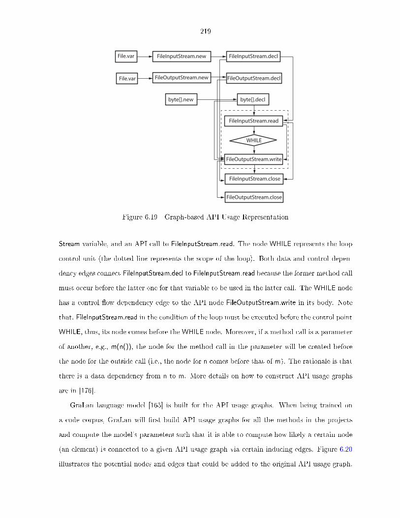
219

FileInputStream.new FileInputStream.decl

FileOutputStream.new FileOutputStream.decl

byte[].decl byte[].new

WHILE

FileInputStream.read

FileOutputStream.write

FileInputStream.close

FileOutputStream.close

File.var

File.var

Figure 6.19 Graph-based API Usage Representation

Stream variable, and an API call to FileInputStream.read. The node WHILE represents the loop

control unit (the dotted line represents the scope of the loop). Both data and control depen-

dency edges connect FileInputStream.decl to FileInputStream.read because the former method call

must occur before the latter one for that variable to be used in the latter call. The WHILE node

has a control �ow dependency edge to the API node FileOutputStream.write in its body. Note

that, FileInputStream.read in the condition of the loop must be executed before the control point

WHILE, thus, its node comes before the WHILE node. Moreover, if a method call is a parameter

of another, e.g., m(n()), the node for the method call in the parameter will be created before

the node for the outside call (i.e., the node for n comes before that of m). The rationale is that

there is a data dependency from n to m. More details on how to construct API usage graphs

are in [176].

GraLan language model [165] is built for the API usage graphs. When being trained on

a code corpus, GraLan will �rst build API usage graphs for all the methods in the projects

and compute the model's parameters such that it is able to compute how likely a certain node

(an element) is connected to a given API usage graph via certain inducing edges. Figure 6.20

illustrates the potential nodes and edges that could be added to the original API usage graph.

220

FileInputStream.new FileInputStream.decl

FileOutputStream.new FileOutputStream.decl

WHILE

FileInputStream.read

FileOutputStream.write

FileInputStream.close

FileOutputStream.close

(1) (a)

(2)(b)

(3)

(c1)

(c2)

Legends:

potential added nodes

potential added edges

Pr (adding (1) + a) = 0.9Pr (adding (2) + b) = 0.81Pr (adding (3)+ c1+ c2 + c3) =...

current nodes

current edges

(c3)

Figure 6.20 Graph Expansion via Graph-based Language Model

For example, after training from the large code corpus, GraLan is able to estimate how likely

the node FileInputStream.new is added via the edge labeled (a), how likely the node FileOutput-

Stream.new is added via the edge labeled (b), and how likely the node FileInputStream.read is

added via the edges (c1), (c2), and (c3). GraLan estimates such likelihoods by observing all

potential expansions from all the API usage graphs seen in a large code corpus. Details on

GraLan's computation can be found in [165].

5. Synthesizing Model. Using GraLan, we develop a novel algorithm to synthesize the API

usage graph that covers as many API elements produced by the mapping model as possible

(Section 6.3.4). In the process, we expand the graph one node at a time based on the proba-

bilities (computed by GraLan) of new API nodes being added to the graph. We start with the

nodes for the pivotal API elements identi�ed by the mapping model. Other nodes are gradually

added based on their likelihoods. We stop expanding if all the API elements produced in the

�rst step are covered or the score is lower than a threshold. Some sub-graphs of the newly

expanded graph involving the new node and edges are seen in the corpus. However, the entire

221

newly expanded graph might not exist in the corpus. Finally, the candidate API usage graphs

are displayed in terms of textual usage templates.

6.3.1.3 API Elements in English Text

To create an alignment between English words and API elements we must �rst identify

from a StackOver�ow post the API elements in freeform English texts and code snippets that

do not necessarily compile. Researchers used simple regular expressions that identi�ed terms by

Camelcase, e.g.,AccountManager is a class. While a slight improvement over IR approaches the

precision and recall remained low 0.33 and 0.64 [17]. RecDoc used a number of sophisticated

resolution techniques including term context to attain a high precision and recall above 0.90 [47].

Performance issues made it impossible for RecDoc to parse large document corpora. In a recent

work, Subramanian et al. suggest a technique that can only parse code snippets and misses API

elements that are in freeform text [219]. In contrast, Rigby and Robillard's automated API

element extractor (ACE) extracts API elements from freeform text and code snippets that do

not necessarily compile with an average precision and recall at or above 0.90 in large corpora

such as StackOver�ow [197].

ACE has three components. First, it has an indexing module for valid API elements. The

index includes not only Android classes and methods, but also Java 7 and other libraries. ACE

is able to identify any Java-based API element that is in the dictionary. Second, a simple

parser that identi�es naming convention, such as Camelcase, and a limited number of language

speci�c constructions, such as the syntax of variable and class declarations. Third the notion of

term context to resolve ambiguous methods and classes. We illustrate the use of each of ACE's

components in an example.

Consider the following post that contains API elements in freeform text, �I'd use toString

to display an Integer as a text.� We parse each token in the post and look it up in the index

of valid API elements. The �rst element we �nd that is in the index is toString(); however,

toString() is overloaded so we need to determine if there is a class in the context, i.e. in the

post, that declares it. We continue to parse the text and �nd the term Integer which is in class

in the index. We then look to see if Integer de�nes any of the ambiguous methods in the post.

222

In our index we �nd that it declares Integer.toString() so we can successfully determine the

declaring class of toString() is Integer. If there is no declaring class in the immediate post

context, we expand the context to include other posts in the thread, i.e. the question and other

answers. In the case that two classes declare a method in the same context, we take the one

that has the closest proximity to the ambiguous method in terms of number of characters. The

output of ACE is a list of quali�ed API elements for each post. This example is a simpli�cation

of our technique and more details on variable and class identi�cation as well as term context

can be found in [197].

6.3.2 Mapping & API Element Inferring

In this section, we �rst explain how we used IBM Model to produce the m-to-n mappings

for individual words to individual API elements. Then, we will explain our novel algorithm to

infer a bag of API elements relevant to any given textual query.

6.3.2.1 IBM Model for Individual Mapping

We processed the StackOver�ow posts as explained in Section 6.3.1.3 to extract the API

elements in both freeform text and code snippets. We then separate the API elements from the

freeform English text. This separation is needed since we aim to map the words and the code

elements. Otherwise, the embedded API elements will a�ect the mappings of the English words

in the query. Next, we processed the texts. The stopwords are removed; keywords are identi�ed

by a NLP tool named GATE [64]. For example, the keywords for the post in Figure 6.16

include copy, �le, save, destination, path, close, open, etc. Finally, all pairs of texts (excluding

the embedded API elements) and the extracted API elements (including embedded ones and

the ones in the code snippets) are used for training the IBM Model [31]. Let me summarize the

foundation of the IBM Model.

Assume that LS and LT are two sets of sequences in two languages, and s = s1s2...sm in LS

and t = t1t2...tl in LT . The goal of IBM Model is to compute the probability P (s|t), that is, the

probability that s is the corresponding of t given the observable t. To do that, IBM Model [31]

considers s to be generated with respect to t by the following generative process. First, a length

223

1 function Infer(Text T = t1t2...tn, TrainedModel M, Data D)2 BagOfElements C = ∅;3 Element c = ChoosePivot(T, M);4 C = C ∪ {c};5 C' = ExpandBag(T \ C, P = {c}, D);6 C = C ∪ C';7 return C;8

9 function ChoosePivot(Text T=t1t2...tn, TrainedModel M)10 Phrases = DetectKeyPhrases(T);11 foreach Ph in Phrases12 foreach word tk in Ph13 Ck = {c | c is mapped with tk};14 Cp = {c | c = argmax |{Ck|Ck 3 c }|, c∈ ∪Ck , k =1..n};15 C∗ = ∪Cp;16 c' = argmax

∏(#mappings (tk, c') / #(c' in training data), c'∈ C∗, tk ∈ T;

17 return c';18

19 function ExpandBag(Text T=t1t2...tn, Pivot P = {cp}, TrainedModel M, Data D)20 BagOfElements C = ∅;21 foreach word tk in T22 Ck = {c | c is mapped with tk};23 Initialize scores for all elements in Ck

24 foreach Code c in Ck

25 s = ComputeScore(P, c, D);26 C∗ = {top K elements with highest scores s};27 P = P ∪ C∗;28 C = C ∪ C∗;29 return C;30

31 function ComputeScore(PreviousElements P = {c1,...,cp}, Element c, Data D)

32 return∏

c∗∈P#(c,c∗)#(c∗)

Figure 6.21 API Element Inference Algorithm

m for s is chosen with the probability P (m|t). For each position i, it chooses a symbol tj ∈ t

and generates a symbol si based on tj . In this case, it considers si to be aligned with tj . Such

alignment is denoted by an alignment variable ai = j. The symbol si can also be generated

without considering any symbol in t. In this case, si is considered to be aligned with a special

symbol null. The vector a = (a1, a2, ...am) with the value of ai within 0..l is called an alignment

of s and t (ai = 0 means no alignment in t for ai). IBM Model [31] computes P (s|t) and the

alignments based on those variables (see [31]). We built it on top of Berkeley Aligner [24]. The

result of training is the m-to-n alignments between individual words and API elements.

224

6.3.3 Infer API Elements for a Given Query

Key ideas. The algorithm uses the result of individual mappings from IBM Model. We design

it with the following key ideas:

1. We do not infer the API elements using the textual similarity between the words in

the query and the API elements. Instead, we use the mappings of individual words and API

elements from IBM Model to bridge the lexical mismatch between texts and code [243] that

have been reported to be a problem for code search and retrieval applications in SE. We rely on

statistical learning on how often they are used in textual descriptions and corresponding source

code.

2. Unlike the previous approaches that treat each word separately, we consider the words

in the query as the contexts for each other in inferring their relevant API elements. First, we

identify key phrases using an NLP tool [64], e.g., �open the contents of the �le� in Figure 6.16.

We next identify the pivotal API elements as the ones with the most mappings with the words

in each key phrase. Each word as individual is mapped to multiple code elements, which might

not �t with the current context. For example, open and contents might refer to the API elements

di�erent from the one for �le manipulation. If the word �le is also considered, the pivotal API

elements can be more precisely identi�ed. For example, the overlapping API elements could

be FileInputStream.open and FileOutputStream.open. The scores of mappings are considered as

well.

3. Pivotal elements are used to expand the bag of API elements. We further consider the

context on the source code side, and speci�cally, the likelihoods of API elements that often

co-occur in the training data. For example, in the phrase �save it to the destination path�

in Figure 6.16, the word save can be mapped to multiple elements. However, since open is

already mapped to FileInputStream.open and/or FileOutputStream.open, we should map save to

FileInputStream.write and/or FileOutputStream.write, based on the observation that the methods

open and write of those classes appear together in multiple posts.

4. Our design strategy is to produce as many needed API elements as possible while main-

taining a reasonably low number of them. Otherwise, the graph synthesizing module in the

225

later step could face the scalability issue since it is more computationally costly to expand the

graph to search more needed nodes. Thus, this inferring module favors the coverage of API

elements and expects the synthesizing module to remove the incorrect elements (Section 5).

Details. Figure 6.21 starts with the process of choosing the pivotal API elements. First, we

use an NLP tool [64] to detect the key phrases in the text T (line 10) (e.g., �to save a copy of a

certain �le�, �to open the contents of the �le�, etc. For each key phrase, we eliminate stopwords.

Using IBM Model, we �nd the mappings for all of its words (line 13). We identify the API

elements that have the most mappings to the words in the phrase. Then, we collect all those

API elements for all key phrases (lines 14-16). Note that the API elements that frequently

occur in the training data are penalized via the denominator in the formula on line 16.

Next, the process of expanding starts from each of those pivotal API elements (line 5 and line

19), and the pivotal words that have maximum mapping scores with those elements. Then, we

process remaining words according to their co-occurrences with the pivotal word. We examine

each of its corresponding API elements c and compute the association score (ComputeScore).

The formula on line 32 represents the likelihood of an API element c co-occurring with the

other code elements that have previously identi�ed. The more frequently c co-occurs in the

posts with many previously identi�ed ones, the higher its score (line 32). Then, we collect the

top K elements with the highest scores for each word (line 26). We keep expanding until we

cover all the remaining keywords. Finally, the collected API elements are returned (line 29).

6.3.4 Synthesizing API Usages

6.3.4.1 Overview and Key ideas

The goal of our synthesizing model is to take the bag of relevant code elements produced by

the mapping model and put them together to create an API usage graph relevant to the textual

query. In our solution, we have the following key ideas.

1. Existing approaches often treat code search and API usage recommendation as an IR

searching/ranking problem in which the texts in the query are used to match against the names

of the API elements in an encoded codebase. The API usages in the codebase with the elements'

226

names that textually match the most with the texts in the query will be ranked and returned.

In contrast, we use GraLan [165], a statistical graph-generative approach to synthesize the

(potentially new) API usages that have high regularity and are most relevant to the query.

We use it to learn from a large code corpus the API elements that often occur together in

frequent usages. We then design an algorithm for API usage graph synthesis by maximizing the

likelihoods of those API elements being used together in certain orders and dependencies in the

corpus.

Speci�cally, GraLan computes how likely a certain node (representing an API element) is

connected to a given API usage graph via certain inducing edges. Based on those likelihoods,

T2API synthesizes an API usage graph by expanding it one node at a time and maximizing the

likelihoods of the connections of the API elements. We expect that the resulting synthesized

graph or at least its smaller subgraphs (representing smaller usages) have high regularity.

2. Toward having the synthesized graph with high relevancy to the given query, we use one

of the pivotal API elements identi�ed by the code inferring module (Section 6.3.2) and expand

the graph from it. Those pivots are the key elements relevant to the query.

3. To enable T2API to create a new usage that might not appear as its entirety in the

training data, we support the situation in which the intermediate synthesized graph at a step

might be disconnected (i.e., containing disconnected components). This situation occurs since

smaller, unrelated-yet usages (i.e., subgraphs) might be formed �rst and later connected together

via newly added edges to form a larger API usage in the expansion process. Thus, we allow

an expansion in which we add a node without any inducing edges. Such addition is not allowed

in GraLan, however, is valid in T2API. The score for a disconnected graph is the average score

of its connected components' scores. We assign the score for a connected graph (including a

single-node graph) with its occurrence probability in the corpus.

4. Due to a very high number of possibilities of expansion, we use the beam search strategy

to greedily maintain only the top candidate graphs at each step with high occurrence likelihoods.

227

FileInputStream.new FileInputStream.decl

FileOutputStream.new FileOutputStream.decl

byte[].decl byte[].new

WHILE

FileInputStream.read

FileOutputStream.write

FileInputStream.close

FileOutputStream.close

File.var

File.var

(1)

(11)

(3)

(4)

(5)

(6)(7)

(8)

(9)

(10)

(13)

(2)

(12)

1Step New nodes New edges

FileInputStream.new []2 File.var File.var->FileInputStream.new

12 File.var File.var->FileOutputStream.new

3 FileInputStream.decl FileInputStream.new ->FileInputStream.decl

4 FileInputStream.read FileInputStream.decl->FileInputStream.read

5 FileInputStream.close FileInputStream.read-> FileInputStream.close

FileInputStream.decl -> FIS.close6 byte[].decl byte[].decl->FileInputStream.read7 byte[].new byte[].new -> byte[].decl8 WHILE FileInputStream.read->WHILE9 FileOutputStream.write WHILE->FileOutputStream.write

10 FileOutputStream.decl FileOutputStream.decl->FileOutputStream.write

13 FileOutputStream.close FileOutputStream.write->...close FileOutputStream.decl->...close

The numbers show the ordersof the nodes and inducing edgesbeing added.

{byte[].decl,FIS.read}->FOS.write

11 FileOutputStream.new FileOutputStream.new->FileOutputStream.decl

Figure 6.22 Graph Synthesizing Example for a Candidate Usage Graph

6.3.4.2 Detailed Algorithm

Figure 6.23 shows the pseudo-code of our API usage graph synthesis algorithm. It takes as

input the bag of API code elements B and the GraLan graph-based language model GL (which

was trained on a large code corpus containing Java libraries of interest), and produces a ranked

list of candidate API usage graphs.

First, we use as the starting node the pivotal API element found in the previous step that

has the highest occurrence likelihood (line 4). Then, T2API extends each candidate graph in

CG' (line 10). With the beam search strategy, we pick the graph g with the highest score �rst.

For each remaining API node, we consider it in the order according to the number of its inducing

edges connecting itself to the current graph g. We process the current graph g and the current

node n with the function ExtendGraph. To do that, we ask GraLan to �nd all possible extended

graphs from the current graph g (line 20). If after removing the node n and its connecting edges

from the extended graph eg, we get the exact match to the current graph g (line 23), then we

can ask GraLan for the probability of extending g with the new node n (GetProb(g,n) at line

24). In this case, the score for the newly extended graph eg is computed by multiplying the

score of the current graph g with such probability. If g is disconnected, each of its connected

components is considered. Since we have to prune the extended graphs with low scores, we keep

228

1 function APIGraphSynthesis (ElementBag B, GraLanModel GL)2 Graph g = null;3 GraphList CG = []; // candidate graphs4 P = ChooseAPivot(B);5 g.add(P);6 g. score = GetScore(g);7 CG.add(g);8

9 CG′ = CG;10 while (CG′ <> ∅)11 Remove a graph g from CG′ with highest score;12 Sort(R);//sort nodes according to #edges connecting to g13 foreach Node n in R14 GraphList G+ = ExtendGraph(g,n,GL);15 if (G+ <> ∅) CG = CG ∪ G+;16 return CG;17

18 //Extend g with node n and inducing edges to get new graphs19 function ExtendGraph(Graph g, Node n, GraLanModel GL)20 GraphList EG = GL.FindExtendingGraphs(g);21 GraphList RG = [];22 foreach Graph eg in EG23 if (g = eg n)24 eg. score = g.score × GetProb(g, n)25 if (eg. score in a top list ) RG.add(eg);26 if (EG is empty or g <> (eg n))27 eg = g ⊕ n with eg. score = GetScore(g ⊕ n)28 return RG

Figure 6.23 Graph Synthesizing Algorithm

eg only if its score is in the top-ranked list among other extended graphs at this step (line 25).

If n is not a feasible extended node according to GraLan, we still add it to the current graph

g, hoping that it will be connected in a later expansion (lines 25�27). In this case, our new

graph is disconnected and assigned with a score as explained earlier. We continue to process the

newly extended graphs (line 14) and remaining API elements in R. We stop when all elements

are covered.

Then, in the candidate graphs at the last step, we remove the single, disconnected nodes

since those isolated nodes are likely the ones that were incorrectly included by the code inferring

algorithm in the previous step. Finally, the candidate API graphs are presented.

229

6.3.4.3 Example

Figure 6.22 illustrates the result of each expansion step for the API usage shown in Sec-

tion 6.3.1 (we show only the top-ranked candidate graph). For example, the chosen pivotal node

is FileInputStream.new (1) (among FileInputStream.new and FileOutputStream.new). At step 2,

since in the training data, File.var is likely used as a parameter for an instantiation of FileIn-

putStream, it is newly added and marked with (2). At steps 3, 4, and 5, a variable declaration,

read and close operations are likely to be used on an FileInputStream object, thus the nodes

FileInputStream.decl, FileInputStream.read, and FileInputStream.close are added. Next, since in

the corpus, FileInputStream.read is often used to read data from a �le into an array among which

an array of byte matches with the element byte[].decl in B. Thus, it is added at step 6, leading

to the addition of its instantiation byte[].new at step 7. At step 8, the WHILE node is added

since in the training corpus, the model observes that FileInputStream.read with an array of bytes

byte[].decl often goes with a while loop.

Step 9 is an interesting step because after step 8, we have a small usage for reading into

a �le corresponding to a subgraph (1)�(8): File.var, FileInputStream.new, FileInputStream.decl,

byte[].new, byte[].decl, FileInputStream.read, WHILE, and FileInputStream.close (the nodes are

highlighted in a darker color). At step 9, the node FileOutputStream.write (with a darker bor-

der) is added from WHILE, byte[].decl, and FileInputStream.read because the smaller sub-graph

involving those nodes and FileOutputStream.write occurs frequently. That sub-graph [(6),(4),(8),

and (9)] represents a smaller usage in which a while loop is used to read from a FileInputStream

to a bu�er and write the bu�er's contents to a FileOutputStream. That allows me to expand

to the nodes (10)�(13), which correspond to another usage of writing to a �le via FileOutput-

Stream. Thus, after expanding, we will have a larger API usage. Speci�cally, that expansion

is as follows. At the step 10, FileOutputStream.decl is added because it occurs often before

FileOutputStream.write. At step 11, an instantiation with FileOutputStream.new occurs often

for a declaration of that type. Then, at step 12, File.var is connected because it is used as

an argument for such instantiation. Finally, FileOutputStream.close is inserted because it often

occurs after FileOutputSream.write.

230

Table 6.20 StackOver�ow Dataset for Training Mapping Model

Number of posts 236,919Avg. number of words per post 132Size of word dictionary 701,781Size of API element dictionary 11,834Avg. number of API elements per post 9.2

Avg. number of extracted keywords per post 20.2The number of distinct keywords 103,165

If the occurrence probability of FileOutputStream.new is higher in the training data, it will

be the pivot and the order of nodes being added will be di�erent. The usage of writing to a

�le via FileOutputStream will be formed �rst. Moreover, there could be cases where smaller,

independent usages are expanded. In those cases, we maintain a disconnected graph with its

connected components.

6.3.5 Empirical Evaluation

With our above approach, we have built T2API [2] to synthesize API usage templates for

any given English description of the task. Then, we conducted an empirical evaluation on

RQ1. The accuracy of the code inferring module to infer the relevant API elements from a

given text,

RQ2. The accuracy and usefulness of T2API in API usage template synthesis from given

textual descriptions.

All experiments were conducted on a computer with AMD Phenom II X4 965 3.0GHz, 8GB

RAM, and Linux Mint.

6.3.5.1 Accuracy in API Elements Inferring

Data collection. To be able to infer the bag of API elements relevant to a textual query,

we had to train our mapping model and then used it for inferring algorithm (Section 6.3.3).

To do that, we used the StackOver�ow data collected in our prior research (by Rigby and

Robillard [197, 72]). In the dataset, we used 236,919 entries, each of which has two parts: 1) the

textual descriptions of the usage/purpose of some programming task, and 2) the corresponding

231

bag of API elements that are extracted from the posts (including from its descriptions and code

snippets). The posts and code elements were extracted via the ACE tool [197] as described in

Section 6.3.1.3. As seen in Table 6.20, our data set contains a very large number of posts, with

very large numbers of words and API elements in both dictionaries.

Procedure and Metrics

In this experiment, we aimed to evaluate the accuracy of T2API's inferring module that

outputs a bag of API elements for a given English description on a programming task. We used

the dataset collected from StackOver�ow for this experiment. For each entry, we �rst processed

the textual description. We removed the stopwords, grammatical words and punctuation. We

performed word stemming and extracted the keywords using GATE [64]. To train our mapping

model, in each entry, we need to remove the extracted API elements from the textual description

to allow the computation of mappings from texts to code. Otherwise, the embedded API

elements would hinder that computation due to the mappings from code to code. After our

preprocessing, we collected 103,165 distinct keywords with 20.2 keywords per post. For training,

each entry now contains a list of keywords and a bag of API elements. We used all 236,919

entries after preprocessing to train IBM Model using Berkeley Aligner tool [24]. The output of

IBM Model is the m-to-n mappings for individual words to individual API elements. After this

step, each word is mapped on average to 16.46 API elements. This step is very helpful since

it allows our inferring algorithm (Section 4.2) to consider a number of potential API elements

much smaller than the size of API element dictionary (11,834). A small number of API elements

also helps in reducing noises and making our synthesizing algorithm in the later step scalable.

To collect the testing posts/entries, we randomly selected from the StackOver�ow data

set [72] 250 post samples that satisfy the following: 1) they do not belong to the posts that

were used during training, 2) a post has high rating on its answering texts, and 3) a post

contains one code snippet. The �rst condition is the principle of cross validation. The second

one allows me to have a fair evaluation. The third condition is needed because we used the

code snippet as the ground truth against which we compared the synthesized API usage in a

later experiment. In those 250 posts, the average number of words and API elements per post

are 7.99 and 4.4, respectively.

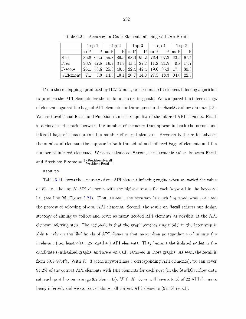
232

Table 6.21 Accuracy in Code Element Inferring with/wo Pivots

Top-1 Top-2 Top-3 Top-4 Top-5no-P P no-P P no-P P no-P P no-P P

Rec 35.8 69.5 55.8 86.5 68.6 96.2 76.4 97.3 82.5 97.4Prec 20.5 47.8 16.2 34.7 13.4 27.2 11.2 21.5 9.8 17.7F-score 26.1 56.6 25.0 49.5 22.4 42.4 19.6 35.3 17.5 30.0#Element 7.1 5.9 14.0 10.1 20.7 14.3 27.5 18.3 34.0 22.3

From those mappings produced by IBM Model, we used our API element inferring algorithm

to produce the API elements for the texts in the testing posts. We compared the inferred bags

of elements against the bags of API elements for those posts in the StackOver�ow data set [72].

We used traditional Recall and Precision to measure quality of the inferred API elements. Recall

is de�ned as the ratio between the number of elements that appear in both the actual and

inferred bags of elements and the number of actual elements. Precision is the ratio between

the number of elements that appear in both the actual and inferred bags of elements and the

number of inferred elements. We also calculated F-score, the harmonic value, between Recall

and Precision: F-score = 2×Precision×RecallPrecision+Recall .

Results

Table 6.21 shows the accuracy of our API element inferring engine when we varied the value

of K, i.e., the top-K API elements with the highest scores for each keyword in the keyword

list (see line 26, Figure 6.21). First, as seen, the accuracy is much improved when we used

the process of selecting pivotal API elements. Second, the result on Recall re�ects our design

strategy of aiming to collect and cover as many needed API elements as possible at the API

element inferring step. The rationale is that the graph synthesizing model in the later step is

able to rely on the likelihoods of API elements that most often go together to eliminate the

irrelevant (i.e., least often go together) API elements. They become the isolated nodes in the

candidate synthesized graphs, and are eventually removed in those graphs. As seen, the recall is

from 69.5�97.4%. With K=3 (each keyword has 3 corresponding API elements), we can cover

96.2% of the correct API elements with 14.3 elements for each post (in the StackOver�ow data

set, each post has on average 9.2 elements). With K=5, we will have a total of 22 API elements

being inferred, and we can cover almost all correct API elements (97.4% recall).

233

Table 6.22 Statistics of Dataset for Training the Graph Synthesizing (Language) Model

Number of projects 543

Number of source �les 29,524Number of methods 317,792Number of extracted graphs 284,418,778Number of unique graphs 82,312,248Number of unique API elements 113,415

Despite the low precision due to the redundantly generated elements (we will explain the

causes later), we found that our graph synthesizing model is indeed capable of removing them

as we will show such result in the next section. Finally, for practical use, one must consider

the trade-o�s between recall and the number of inferred elements as well since more elements

are generated, recall increases, however, the running time of graph synthesizing model might

increase due to the exploration of many more graphs.

6.3.5.2 Accuracy in API Usage Graph Synthesis

In this experiment, we aimed to evaluate the overall accuracy of T2API (combining all

modules) in synthesizing from an English description to the API usage graph.

T2API's synthesizing model (Section 6.3.4) needs to be trained on a large code corpus via

GraLan [165] before we can use T2API to synthesize API usage graph. Thus, we collected a set of

Java and Android projects from GitHub. We selected the projects with well-established histories

so that their code is compiled and can be semantically analyzed to build usage graphs. Table 6.22

shows the statistics of the data set. In general, we collected a very large number of API usage

graphs (284M) with 82M unique graphs and 113,415 unique API elements. For testing, we used

the same StackOver�ow data set of 250 posts as in the previous study (Section 6.3.5.1).

Procedure and Metrics

For each testing post, we used its description with embedded elements (but excluding code

snippets) as a query for T2API. T2API's inferring module processed the text and inferred

the bag of elements, which are passed to the synthesizing module to produce the candidate

synthesized graphs. For the result from the inferring module, we chose K=3 in this experiment

234

Table 6.23 Accumulative Accuracy

Actual Syn Actual ∩ Syn Rec Prec

Nodes 1,417 2,146 1,243 87.7% 57.9%Edges 1,699 2,332 939 55.3% 40.3%

Table 6.24 Graph Synthesizing Accuracy

Recall Precision

100% >=70% 100% >=70%

Nodes 147 (58.6%) 234 (93.2%) 49 (19.5%) 134 (42.6%)Edges 67 (26.7%) 134 (53.4%) 43 (17.1%) 82 (32.7%)Both 63 (25.1%) 126 (50.2%) 20 (8%) 40 (15.9%)

because it gives a high recall value with a reasonable number of API elements. We used the

single code snippet in the post as the ground truth for comparison. For each synthesized graph

gsyn, we compared it against the graph g built from the snippet, and measured the traditional

IR metrics Precision and Recall for the bags of nodes and edges. Recall on nodes is de�ned as the

ratio between the number of shared nodes in g and gsyn and the number of nodes in g. Precision

on nodes is the ratio between the number of shared nodes in g and gsyn over the number of

nodes in gsyn. Similarly, we can de�ne Recall and Precision on edges.

T2API can give a list of candidate synthesized graphs. However, as in machine translation,

we measured accuracy metrics only on the synthesized graph with highest score for each testing

post.

Results

Table 6.23 shows the accumulated accuracy over all the synthesized graphs. In general,

T2API can generate almost 90% of the nodes in the code snippets, with almost 60% precision.

55.3% of the dependencies are covered in our graphs.

To investigate further, we compute accuracy for individual synthesized graphs. Each graph

is the result for a testing post. Tables 6.25 shows the distributions of Recall and Precision values

for nodes and edges over all the synthesizing graphs for all testing posts. Table 6.24 shows

the numbers and percentages of the synthesized graphs with high accuracy. The numbers

235

Table 6.25 Precision and Recall Distributions for Nodes and Edges over 250 Testing Posts

Nodes < 50% 50-70% 70-80% 80-90% 90-100% 100%

Rec 14 (5.6%) 16 (6.4%) 26 (10.4%) 25(10%) 36 (14.3%) 147 (58.6%)Pre 76 (30.3%) 68 (17.1%) 26 (10.4%) 17 (6.8%) 15 (6%) 49 (19.5%)

Edges < 50% 50-70% 70-80% 80-90% 90-100% 100%

Rec 66 (26.4%) 51 (20.3%) 19 (7.6%) 35 (13.9%) 13 (5.2%) 67 (26.7%)Pre 115 (45.8%) 54 (21.6%) 22 (8.8%) 8 (3.2%) 9 (3.6%) 43 (17.1%)

and percentages in the table show the numbers of synthesized graphs and their corresponding

percentages in 250 testing posts, respectively.

The result re�ects well our strategy to cover as many needed nodes (API elements) as

possible. This high recall for nodes is important because developers do not need to spend much

time to search for the missing nodes. As seen, in 147 posts (58.6%), all the nodes in the oracle

code snippets are covered in our synthesized graphs. In 93.2% of the cases, recall for nodes are

higher than 70%, i.e., the missing nodes are about 2 nodes on average for each code snippet in

a post. The precision on the nodes is reasonable in which 42.6% of the cases, more than 70%

of the suggested nodes are correct.

As seen, the synthesizing module is able to improve (node) precision over the inferring

module (from 27.2% to 57.9%) by removing the API elements irrelevant to others in a usage

(but produced by the inferring module). The recall for edges are reasonable with 53.4% of

graphs missing less than 30% of the edges. However, we expect that developers can concretize

the template variables in our usage template and their uses, which automatically creates data

dependencies. For example, T2API produces File.var and FileInputStream.new. Despite missing

the edge connecting them, when concretizing the variable for a File, (s)he will be able to use it

as the argument of the FileInputStream's constructor. Moreover, T2API is able to synthesize 63

graphs (25% of the cases) with 100% recall. In half of the cases, the missing nodes/edges are

less than 30%.

However, the precision values for both nodes and edges are low. There are three key reasons.

First, as explained, our synthesizing module aims to produce as high recall for nodes as possible.

We expect that developers can examine the nodes if they need them. The second reason is the

236

fact that T2API added into the synthesized usage the API calls that need to be called �rst as an

initial preparation step for the use of the code snippet in the post. In those cases, despite having

imprecise nodes (according to the code snippet), the extra API elements are in fact part of the

real correct usages. Thus, as part of our empirical evaluation, we also conducted a survey with

human subjects to verify the usefulness of the API graphs/templates. Finally, other factors for

imprecision will be discussed later.

6.3.5.3 Web-based Survey

We created a survey and asked 10 human subjects who are SE graduate students at Iowa

State University and Concordia University, and have experience in Java programming for more

than 4 years to evaluate the results. None was involved in the project.

Each subject was shown a StackOver�ow post including the title, textual descriptions, and a

code snippet. We also showed them the synthesized API usage graph and the textual template.

The template is a sequence of the labels of the API elements in the graph where the orders

among API elements are preserved. For example,

1. Location varLocation

2. Location.getLongitude(...)

3. Locale.getDefault(...)

4. new Geocoder(...)

5. Locale varLocale

6. Geocoder varGeocoder

7. Location.getLatitude(...)

8. Geocoder.getFromLocation(..)

9. List varList

10. List.size(...)

11. List.get(...)

12. Address varAddress

13. String varString

14. Address.getMaxAddress..(..)

Due to the space limit, we do not show the corresponding graph in this paper. Next, we

asked them to give a rating for the result on whether it is �useless�, �useful and could be a good

starting point�, �very useful�, and �more useful�. �Useless� means that the template is totally

incorrect and useless. �Useful and could be a good starting point� means that the template might

need a reasonable amount of modi�cations to correct the orders or API elements. �Very useful�

means that the template is correct and can be used as-is. �More useful� refers to the cases in

237

which the template contains additional contextual elements not mentioned on StackOver�ow,

but required to prepare as the initial declarations or method calls before using the code snippet

as a template. Each participant graded 25 results. In total, we have the ratings for 250 usages.

The result is as follows:

Useless Good Starting Point Very Useful More Useful Total

19.6% 43.2% 27.6% 9.6% 100%

49 108 69 24 250

Overall, the participants found that 27.6% of the templates have correct elements in correct

orders, and 43.2% of them are not correct but are good starting points. Interestingly, in 9.6%

of the cases, the participants found that the synthesized templates contain additional calls

useful. For example, in the post 11271458 [216], an answer contains only the code snippet

to use Geocoder to get the current location zip code. However, the author of the answer did

not include the code to prepare a Location object to get the latitude and longitude to be

used in the method Geocoder.getFromLocation. In this case, T2API saw in the database that

Geocoder.getFromLocation often goes with Location.getLongitude and Location.getLatitude, thus,

synthesized them in a usage (see the template in Section 6.3.5.3). There are 24 �More Useful�

cases that were not listed as correct, but in fact, are very useful in containing additional correct

information.

Finally, 85% of the synthesized graphs (not shown) do not exist as a whole in the training

data. Thus, this shows T2API's capability to generate new graphs from smaller already-seen

subgraphs.

6.3.6 Limitations

This work is part of our e�ort toward synthesizing/generating source code from textual

descriptions. We started with API usage synthesis since API usages are well-studied in SE. Our

result shows that this direction is promising because from textual descriptions, our tool is able

to produce a good and useful starting point of API code templates in a reasonably large number

of testing queries. During the process, we have learned the following lessons on the limitations.

First, as in any other machine translation approaches, high-quality training data is crucial. In

238

Table 6.26 Time and Space Complexity

Inferring Model T2API

Storage 2.5GBs/236K posts 3.7GBs totalTraining time 8hrs/236K posts 45 hrs/543 projectsSuggestion time 0.08 seconds/post 11.2 seconds/post

NLP, where the corpora of parallel texts in two languages have been (semi-)automatically or

manually built with human annotations and veri�cation. Unlike that, there does not exist a

high-quality training corpus of textual descriptions of tasks and the corresponding API usage

or code in general. We used StackOver�ow posts and their code snippets and embedded code

elements. The quality is reasonable, however, not the best. In many posts, the texts might not

describe the task in the code snippet. Moreover, the code snippets might not be compiled and

often lack of type information. Thus, those factors a�ected T2API's accuracy. In the future,

as a community, we might need to �nd an e�cient way to build better corpora for this line of

research. StackOver�ow is a good starting point for that purpose.

T2API currently relies on statistics of API elements that often go in the code snippets or the

texts of the posts, and on the graph language model, GraLan [165]. Accuracy could be improved

much if we can integrate NLP techniques to process the semantics of the texts. At the same

time, program analyses on the source code could also be integrated to adjust the generation

process of the nodes and graphs for the synthesized usages. Currently, there is no semantic

analysis on both sides. Perhaps, the rule-based approaches [97] that have been successfully

used in code migration could be explored.

Expanding T2API beyond API usage templates is challenging. We need better representa-

tions that can capture well the semantics of natural-language texts and source code, and are

suitable for automatic aligning/mapping between them. That depends much on the pairs of

natural and programming languages. Therefore, the applicability to the languages other than

Java is also not straightforward.

239

Time and Space Comlexity. Table 6.26 shows T2API's time and space complexity. Training

time is a drawback from T2API. However, one can train T2API o�ine for suggestion later. As

seen, the suggestion time for a query is only 11.2s. Storage cost is quite reasonable.

Threats to Validity. Our collected data set might not be representative. The quality of the

posts varies. However, we tried to use the posts with high ratings. Using the code snippet as the

ground truth poses the threat to the result because the texts and the snippet might be loosely

related. The metrics of recall and precision do not re�ect well the quality of the template. Thus,

we conducted a small survey on the users' opinions. More full-scale empirical study is required

to study the usefulness of the tool. There is possible construct bias as we chose the Java and

Android APIs. In our survey, human errors could occur. It su�ers from selection bias, as not

all participants have the same level of expertise on the API usages.

240

CHAPTER 7. RELATED WORK

7.1 Empirical Study on Naturalness and Repetitiveness

There are several empirical studies on the repetitiveness of source code. Early research shows

that a signi�cant percentage (7�23%) of the source code in a project has been cloned [19]. Roy

and Cordy [201] studied on 15 open-source projects and reported that 7.2�15% of code is clones

at the function level. Our study is in a much larger scale. Moreover, we look at the PDG, rather

than comparing only syntactic units as in their study. At the �le level, Mockus et al. [155, 156]

study on 13.2M source �les, and report more than 50% of the �les being used in multiple

projects. At a �ner granularity, Kapser and Godfrey [108] reported that up to 10�15% of source

code in a project can be code clones. Gabel and Su [63] conducted a large study on uniqueness

of source code at the token level. They reported that at the granularity level of 6 tokens,

50�100% of the code of a project is repeated. Hindle et al. [82] compute the cross-entropy for

source code to show that code is repetitive at the lexical level. Barr et al. [21] reported a high

degree of graftability of code changes, providing a foundation for program auto-repairing.

Our prior study on repetitiveness of changes is at the AST level [169]. In comparison, in this

study, we focus on source code, rather than changes. In this study, we studied repetitiveness,

composability and containment of routines at PDG level. Our API usage graph (Section 2.2)

and vector representation (Section 3.2) are re-used from our prior work [176, 171]. The graph

query infrastructure (Section 3.1) was built for this study.

As in several previous studies, we use PDG as the representation for program's semantics.

GPLAG [125] detects cloned code via mining PDG with an approximated subgraph searching

with a statistical lossy �lter to prune the search space. Duplix [119] �nds similar subgraphs in

PDG to detect clones. Their approximated algorithm was run on 13 projects with 2K-24KLOCs.

241

Komondoor and Horwitz [116] use program slicing and graph matching on PDG. To scale up, we

used hashing on vectors before pairwise comparison. In contrast, Gabel and Su [61] map PDG

subgraphs to structured syntax and reuse Deckard [100] to detect clones in AST. Portfolio [141]

is a tool to �nd relevant functions and their usage. Mendez et al. [146] studied the diversity in

how classes in API libraries are used.

There are several excellent literature surveys on clone detection techniques [202, 25]. Gen-

erally, the approaches are classi�ed based on their code representations. The typical categories

are text-based [53, 137], token-based [20, 107, 122, 145], tree-based [23, 100, 58], and graph-

based [116, 125]. Many clone detection tools focus on individual projects, rather than across

projects as in our study. There have been several empirical studies on code clone changes [111],

cloning across projects [5], API usages [232, 123, 157], etc.

Several approaches use the data structures such as pairs, sets, trees, and graphs to model

abstractions in code and then detect patterns in API usages and examples [143, 157, 154, 34,

140]. Deterministic pattern mining methods are used, e.g., mining frequent pairs, subsequences

[233, 4, 251], item sets [33], subgraphs [176, 39], association rules [128].

7.2 Language Models

The statistical n-gram language model [136] has been used in capturing patterns in source

code [82, 95]. Hindle et al. [82] use n-gram model on lexical tokens to suggest the next token.

In SLAMC [174], we enhanced n-gram by associating code tokens with roles, data types, and

topics. Tu et al. [227] improve n-gram with caching for recently seen tokens to improve next-

token suggestion accuracy. Raychev et al. [193] capture common sequences of API calls with

per-object n-grams to predict next call. We do not compare GraLan to SLAMC [174], Tu et

al. [227], and other code completion methods [82] because GraLan works at the API level, rather

than the lexical level.

Allamanis and Sutton [9] present a token-based probabilistic language model for source code.

Hidden Markov Model is used to learn from a corpus to expand abbreviations [76].

Deterministic pattern detection. Many approaches use such data structures as pairs, sets, trees,

and graphs to model various abstractions in code. Deterministic pattern mining methods are

242

used, e.g., mining frequent pairs, subsequences [233, 4, 251], item sets [33], subgraphs [176, 39],

associate rules [128].

Code completion based on mined patterns. Bruch et al. [33]'s best-matching neighbor approach

uses as features the set of API calls of the current variable v and the names of the methods

using v. The set features in the current code is matched against those in the codebase for

API suggestion. FreqCCS [33] suggests the most frequent call and ArCCS [33] mines associate

rules on API calls. Grapacc [166] mines patterns as graphs and matches them against the

current code. In comparison, Grapacc uses deterministic subgraph pattern mining. Statistic-

based GraLan considers all subgraphs, thus requires higher computation/storage. While trying

to complete a largest pattern as possible, Grapacc cannot suggest smaller subpattern. GraLan

potentially can by using its subgraphs as explained.

There exist deterministic approaches to improve code completion/suggestion and code search

by using recent editing history [199, 86], cloned code [81], developers' editing history [110], API

usages, examples, and documentation [143, 157, 154, 34, 140, 220], structural context [85],

parameter �lling [246], interactive code generation [180], speci�cations on constraints between

input and output [195, 217], etc.

7.3 Code Recommendation

Code Completion. Bruch et al. [32] propose three code completion algorithms to suggest the

method call for a single variable under editing based on code examples in a database. The �rst

one, FreqCCS, suggests the method that is most frequently used in the database. The second

one, ArCCS, mines the associate rules A→ B in which if method A is used, method B is often

called and will be suggested.

In contrast to mining a single, most frequently used method call in FreqCCS and the most

frequent pair of method calls in ArCCS, GraPacc suggests the usage patterns (i.e. most fre-

quently used graph-based API usages), which contain all involved method calls, variables, and

control structures of the usages. Thus, GraPacc represents better the current context. Such

context is important in code completion (Section II). The features in FreqCCS and ArCCS

correspond to individual nodes (for method calls) and individual edges (for pairs of calls) in

243

our Groum. Importantly, GraPacc can handle multiple variables in one or multiple types, while

they focus only on completing the method call for the single variable under editing.

The third algorithm, BMN (best-matching neighbors), adapts k-nearest-neighbor algorithm

to recommend for a variable v. BMN encodes the current context and the examples in the

database as binary feature-occurrence vectors [32]. The features for a context are the un-

ordered set of method calls of v in the currently edited code and the names of the methods that

use v. The set of vectors of examples with the same smallest Hamming distance to the query

vector is called the BMN set. Then, BMN ranks the methods based on their frequencies in the

examples in the BMN set.

In comparison, GraPacc has several key advances over BMN. First, GraPacc captures richer

contextual information of the code under editing, with all ordered method calls, multiple vari-

ables, and control structures in API usages, while BMN represents a context by an un-ordered

set of method calls of a single variable. Second, with the use of API patterns (i.e. correct

usages) as a guidance for code completion, GraPacc can make better context-sensitive method

call completion when there exist alternative patterns (Section II). Importantly, it can handle

multiple variables in di�erent types in a usage. Finally, with API usage patterns, GraPacc

recommends more code elements.

Hill and Rideout [81]'s code completion approach relies on code clones. It matches the

fragment under editing with small similar-structure code clones, and then performs transforma-

tions for code completion. GraPacc leverages code similarity at the API-usage level. Robbes

and Lanza [199] propose 6 strategies to improve code completion using recent histories of mod-

i�ed/inserted code during an editing session. GraPacc has an advance in supporting code

completion for multiple variables in di�erent types, while their approach focuses on a single

method call. Eclipse [54] and other IDEs [91, 89] complete for the call of a variable. Eclipse

supports template-based completion for common constructs/APIs (for/while, Iterator) without

considering the context.

Example Code Search. MAPO [252] mines and indexes API usage patterns and recommends

the associated code examples. It does not support auto-completion. Its pattern is sequential

rules of method calls. It does not progressively update resulting patterns as context changes.

244

Strathcona [85] extracts the structural context of the code under editing and �nds its relevant

examples. It does not aim for code completion. Structural context includes inheritance rela-

tionships, overridden methods, and caller/callee methods of current code. Mylyn [110], a code

recommender, learns from a developer's personal usage history and suggests related methods.

Personal usage history and structural context could provide the useful guide for GraPacc.

Code searching techniques based on program analysis include Prospector [134], XSnip-

pet [204], PARSEWeb [224], Reiss [196]'s. Other approaches use information retrieval [112,

66, 69, 244]. Static analysis is used to extract API patterns into �nite state machine [233],

pairs of calls [55, 127, 236], partial orders of calls [4]. Other pattern mining approaches include

[62, 241, 12, 210, 190, 128, 11, 80, 126].

7.4 Code to Code Translation

Language Migration. Spice [242] translates Smalltalk to C by creating runtime replacement

classes realizing the same functionality of Smalltalk classes. Van Duersen and Kuipers [229]

proposed a method to identify objects by semi-automatically restructuring legacy data struc-

tures. This can be used in migrating from a structural language into an OO one. Other tools

use wrappers [22] or language-independent representations and deterministic rules [234, 159, 78,

209, 52, 93, 238, 178, 101]. MAM [250] mines API mappings via Transformation Graphs. Our

prior work, StaMiner [164], used statistical learning to mine API mappings. The resulting map-

pings are used to enhance the rule-based migration tool Java2CSharp [97]. Sudoh et al. [221]

proposed a method that separately translates clauses in the source sentence and reconstructs

the target sentence using the clause translations with non-terminals.

API Mappings. To mine API mappings, MAM [250] uses API Transformation Graphs, which

describes inputs/outputs and names of API methods and helps compare APIs via similar names

and calling structures. HiMa [148] aggregates the revision-level rules to obtain framework-

evolution rules. Aura [237] uses call dependency and text similarity analysis to identify change

rules for one-replaced-by-many and many-replaced-by-one methods. Both Aura and HiMa share

the textual similarity principle. Twinning approach [177] allows users to specify migration

245

changes to use new APIs. Rosetta [65] needs pairs of functionally-equivalent applications.

StaMiner [164] uses IBM Model [31] to mine API mappings. A comparison was in Section 6.

jv2cs is also related to API adaptation where developers need to migrate their code to

use a new version of libraries/frameworks. SemDi� [46] mines API adaptation changes from

the code of the library itself and other client code. CatchUp [79] records the refactorings to

the library's code and replays them in the client code. Di�-CatchUp [239] use the client code

of APIs to mine API replacements. Others [223, 148] infer transformation rules from client

code. CodeHow [132] searches API usages via extended boolean model. Enery-greedy API

patterns [124] are also mined from Android apps.

Researchers have aimed to derive systematic changes to be reused. Repertoire [192] iden-

ti�es ported edits by comparing the content of patches. Negara et al. [162] discover frequent

code change patterns from code edits. LASE [147] automates similar changes from exam-

ples by creating context-aware edit script, identifying the locations and transforming the code.

SmPL [182, 120, 13] is a transformation language that captures textual patches with a semantic

change.

mppSMT [168] uses a phrase-based, statistical machine translation (SMT) method to mi-

grate Java code to C#. It uses a data-driven approach to avoid the manual process of de�ning

API migration rules in the rule-based migration tools [97, 209, 52, 93, 238, 178, 101]. Karaivanov

et al. [109] enhance phrase-based SMT with grammatical structures. SMT is also used to create

pseudo-code from code [179].

Recently, researchers have applied statistical NLP techniques to source code. Allamanis et

al. [7] propose to suggest method/class names. The code tokens with statistical co-occurrences

are projected into a continuous space together with the text tokens from the names. The

model learns which names are semantically similar by assigning them to locations such that

names with similar embeddings tend to be used in similar contexts [7]. In comparison, we

use Word2Vec and we need to learn the transformation between two spaces, while their model

works in the same space. Moreover, jv2cs works on the abstraction level of API elements, rather

than names of tokens. Maddison and Tarlow [133] use probabilistic context free grammars and

neuro-probabilistic language models but for one language.

246

Researchers have proposed to use language models to suggest the next tokens or API calls [82,

227, 193, 235, 165]. n-gram is used to �nd code templates [95], for large-scale code mining [9], for

model testing [226], etc. White et al. [235] applied RNN LM on lexical code tokens to achieve

higher accuracy than n-gram. Mou et al. [160] propose a tree-based convolutional neural network

(TBCNN) for source code. Allamanis et al. [10] use bimodal modeling for short texts and source

code snippets. NATURALIZE [6] suggests natural identi�er names and formatting conventions.

jv2cs is inspired from a work by Mikolov et al. [151] where similar geometric arrangements were

observed in English and Spanish words for numbers and animals. Our early result on jv2cs was

published in a poster [173].

API Migration. As software is ported to use a new library, developers have to migrate their

code. To mine API migration rules, AURA [237] combines call dependency and text similarity

analysis to identify change rules for one-replaced-by-many and many-replaced-by-one methods.

HiMa [148] matches each revision pair of a framework and aggregates revision-level rules to

obtain framework-evolution rules. Twinning [177] allows users to specify changes that migrate

a program to use new APIs. There are approaches to support adaptation to client code as

libraries evolve [41, 46, 79]. SemDi� [46] mines API usage changes from client code or the

library itself. Di�-CatchUp [239] recognizes API changes and suggests API replacements based

on framework examples. Generalized transformation rules are inferred from examples [223].

SmPL [13, 182] is a domain-speci�c transformation language for a semantic change description.

Statistical Language Models. Hindle et al. [82] used n-gram [136] with lexical tokens to show

that source code has high repetitiveness. Han et al. [76] used Hidden Markov Model to infer

the next token from user-provided abbreviations. n-gram is also used to �nd code templates

relevant to current task [95].

7.5 Text to Code Translation

Information retrieval (IR) approaches. Traditional code search engines (Black Duck Open

Hub [27], Codase [42]) often use simple work matching. Other IR-based approaches allow users

to use natural language texts as a query and match using keywords on components [90], and

247

program structures (e.g., Sourcerer [18], Gridle [188]). Other research enhances IDEs with

searching capabilities on code-related web pages [208, 29].

Other group of IR-based code search approaches considers the relations among API elements

in suggestion [249, 70]. Random walks [207] and PageRank [188] have been used in considering

how methods in classes are called and used to support method searching. McMillan et al. [144]'s

approach �rst locates a set of APIs that are textually similar to the query and then �nds code

examples cover most of them. Portfolio [142] considers also the context of call graphs when

taking given texts as queries. Refoqus [75] is trained in a sample of queries and relevant results

and automatically recommends a reformulation strategy for a given text query to have better

retrieval accuracy. Chan et al. [37] models API invocations as an API graph and �nds the

connected subgraphs that have nodes with high textual similarity to the query phrases. In

comparison, T2API learns the relevant API elements via statistical learning (without textual

matching) and ensembles them via graph-generative language model trained from a large corpus,

thus, can synthesize new API usages.

Program analysis-based approaches. Buse and Weimer [35] use path sensitive data�ow analysis,

clustering, and pattern abstraction to build an automatic tool for mining and synthesizing API

usages from concrete examples. Their approach is not aimed to handle textual queries. It

does not synthesize new API usages from the smaller ones. It generalizes concrete code into

more general/succinct API usages. Sourcerer [18] exploits structural and usage relations to

rank candidates. Other approaches exploits program semantics to retrieve API usages such

as call graphs (FACG [248]) and data/control dependencies (MAPO [251]). Altair [129] and

FACG [248] suggest the similar APIs to the function in the query using common functions

overlapping and weighted API call graph respectively.

Constraint-based approaches. Semantic code search approaches aim to match constraints

given as input. XSnippet [205] supports context-sensitive retrieval for object instantiation.

Other approaches use symbolic execution [218], formal logic and theorem prover to identify

relevant components [184]. Other semantic code search engines execute test cases on candidate

code [121, 195].

248

Parseweb [225] uses control �ow analysis to suggest a sequence of API calls for a query

with the input and output types. Prospector [135] is a technique for synthesizing jungloid code

fragments automatically given a simple query for input/output types. It is able to compose

smaller code to form more complex code fragments. In comparison, T2API is statistical, while

Prospector and Parseweb rely on program analysis to compose code satisfying the types.

Domain-speci�c code synthesis. These approaches use solvers to compose code in domain-

speci�c applications that satis�es given input/output. Typical applications are string anal-

ysis [73], bit vector processing [99, 214], structure manipulation [211], �nite programs with

sketches [212, 213], spreadsheet transformations [77], geometry constructions [74], and hard-

ware design [189]. In comparison, they use partial program analysis on domain-speci�c code,

while T2API relies on statistical learning. They do not handle textual queries.

Statistical approaches in SE. Statistical learning has been used in SE for several applications.

However, none of them supports program synthesis. Typical applications include code sugges-

tion [83, 235], code convention [6], name suggestion [8], API suggestions [194], large-scale code

mining [9], etc. Maddison and Tarlow [133] present a generative model for source code, which is

based on AST-based syntactic structures. TBCNN [160] also uses tree information for suggest

next code tokens. In comparison, T2API uses GraLan, which can capture better program de-

pendencies with graph structures. Allamanis et al. [10] introduce a jointly probabilistic model

short natural language utterances and source code snippets. In comparison, there are two key

di�erences between T2API and that work. First, since they want a joint model for both sides, a

a tree-based representation is used for code and texts. T2API uses graph structures to capture

better control/data dependencies. Second, while their approach uses advanced bimodal model-

ing (e.g., image+text, text+code), we treat code synthesis as a machine translation problem

that allows me to use di�erent language models for texts and source code.

249

CHAPTER 8. FUTURE WORK AND CONCLUSIONS

8.1 Future Work

8.1.1 Empirical

8.1.1.1 Naturalness Code at Di�erent Levels

In chapter 2, I discuss about related work and my work with di�erent levels of code, including

code token, methods and code change. Since source code of a software project can be represents

in di�erent other abstraction levels (project, package, class, block, statements, etc.), there are

other necessary information to study, for example:

1. The naturalness and repetitiveness of API elements. API elements are code ele-

ments written to do speci�c tasks and used repeatedly by di�erent projects (in external

library form). They can have high repetitiveness and entropy. Studying about those char-

acteristics of API is important as it will provide good overview about the usage of APIs

and relating factors which have impacts on using them.

2. The naturalness and repetitiveness of functions/methods in code. Functions or

methods usually implement speci�c tasks in code. There are tasks repeatedly required in

di�erent projects, e.g. printing information. Repeated tasks can be reuse in other loca-

tions (with modi�cation). Hence study characteristics of functions/methods is important.

3. The naturalness and repetitiveness of projects' parts. A software project can

contains di�erent parts, e.g packages, to perform speci�c functionality. The combination

of functionality in parts will perform a complete program. We can study the repetitiveness

and entropy of parts to learn about their regularity and commonality.

250

Overall, those studies are important. They support development of models and applications,

e.g. language model at those level, or level-aware translation.

8.1.1.2 Code vs. Natural Language: Characteristics which are Di�erent be-

tween Code and Natural Language

Although works show that code and natural language have many similar characteristics, it

also reveals di�erence between them. For example, code should always conform syntactic rules.

A list of characteristics can be considered:

• Code should strictly follow syntactic rules over programming language while documents

are more �exible.

• Code has strong hierarchical structure while documents has more �at one.

• and others.

A study about those di�erences is important as it suggests the more advanced techniques

for code processing. In addition a good tool should consider both statistical and deterministic

aspects of programming language and source code. For example, a translation tool should

consider syntactic rule to ensure better translation. Such tool can be called syntactic - aware

tool.

I also interest in the question of where statistical approach is better used than deterministic

approach and where it is not.

8.1.2 Models

8.1.2.1 Advanced Structure-based Model

Graph-based Language Model with Advanced Properties

GraLan (sections 3.6 and 5.3) is my work on graph-based language model. It has advantage

of simplicity. However, it is based on the assumption of conditional independence between

context graphs. And the generation process only considers new generated graph by adding

251

nodes, not inducing edges. Although the models with those assumptions still work well (5.3,

6.3), one can argue that more advance technique can give more bene�t and improve quality.

The improvements can be considered with di�erent aspects:

• Relaxing assumption about independence by analyzing the relationship between graphs.

• Constructing a model that actually generate graph, not adding nodes and inducing graphs.

• Using advance technique like �ltering, outlier removal.

• Enriching context information via considering distance between graphs.

Tree-based/Graph-based for Statistical Translation

Recently in statistical translation in NLP, there exists works employing structure information

of sentences ([240], [247]). Their goal is to take into consideration about grammar between

languages, to enhanced the order of translation.

In code translation, di�erent syntactic rules between languages also play important roles.

Moreover, syntax tree in code can be determined explicitly and exactly, which can support

better for translation. Thus, using and improving tree-based translation models in NLP can

improve much code translation quality.

Besides that, graph representation in code is also important and contribute much infor-

mation. For example, dependency graphs can show dependency and order between elements

in program, which decide how program works. A model for graph-based translation can be

necessary in the future.

Direct Text-to-Graph and Graph-to-Text Translation

T2APIis designed to translate from textual documents corresponding graphs of API ele-

ments. It is based on two steps: 1. Mappings text to a set of API elements and 2. Using a

graph-based language model to generate the graphs. That two-step procedure is common in

statistical translation model (SMT). However, recent research using recurrent neural networks

(RNN) in NLP shows that sentences in one language can be translated to corresponding ones in

another language with only one uni�ed step ([40]). The quality of this approach show signi�cant

improvement. They also design models for translating image to text ([230]).

252

It is reasonable to design models which directly translate from text to graph or graph to

text. One feasible approach is to combine RNN and structured deep neural network models.

8.1.2.2 Advance Neural Network Model

Recently, language and translation models in NLP using deep neural network achieve the

best results, outperform all other approaches. Moreover, studies also show that deep neural

network model can capture semantic information, both about global and local aspect. RNN-

based models can easily capture information in very long sentences. Those features are really

important for programming language processing where source code classes/methods can be very

long and contain elements that have impact to all other elements in them.

Besides that, deep learning models are proved advance in application where linking between

di�erent spaces like image - document, since the can learn mapping via di�erent abstraction

layers. In software development and maintenance, there exists various cross-space linking like

linking between documents and source codes and linking between commit logs and changes.

That is, it will be very interesting to develop DNN-based models to support source code

processing.

8.1.2.3 Hybrid Model

The works presented in this paper revealed the usefulness of statistical-based approaches in

programming language and source code processing, especially where the data is ambiguous and

the regularity is found, especially regularity with large-scale data. Deterministic approaches

have been used successfully in many problems, like program analysis, testing, etc.

A good model should take into consideration both the deterministic and statistical aspects

of data and chose the best scheme for combining them. For example, in code recommendation,

a tool can consider both the n-gram model and the feasible variables for recommending a

parameter.

253

8.1.3 Applications

8.1.3.1 Advanced Code Recommendation

The new code recommendation can recommend not only one token but also many tokens at

once. Moreover, the tool can give summary of recommended code based on translation/summary

models.

8.1.3.2 Code Synthesis and Generation

Automatic code synthesis is important. It can be used to generate new code based on

speci�cation or requirements. It also can be used to simulate, replicate speci�c tasks. In

far future, automatic code synthesis can help user produce program without knowledge about

coding. We can use deep learning models described previously for code synthesis. Another

application is to combine multiple elements from di�erent source, like code transplantation.

Code generation is similar to code synthesis but at higher abstraction level.

8.1.3.3 Code Summary

In maintenance problem, developer need code summary to understand better code, especially

when the code is complex with di�erent levels. There exist various approaches in code summary.

I want to study the application in di�erent way, i.e. consider it a translation problem from source

to textual document. A tool will at �rst analyze code to useful information then use SMT or

DNN models to translate it to text. However, mapping is not simple 1-1 as code contains many

elements while document contains small number of tokens.

8.1.3.4 Code Quality Evaluation and Bug Detection

In NLP, irregularity can be used to estimate code quality. For example, model can be used

to detect if an word B should appear after another word A. If in common use, B never appears

after A, the appearance of B after A can lead to suspect. An application can be used for detect

irregularity in code. For example, in Java, if a token ( appears after a token ), it should be an

irregularity.

254

8.1.3.5 Automatic Code Maintenance Function

In NLP, there is research on automatic �xing of documents. We can extend use of language

model for �xing, change code according to learned regular code. Automatic code maintenance

is also relating to activity like code refactoring, code restructuring which support code improve-

ment. In those cases, machine learning can learn to automatically evaluate and tuning code for

code improvement.

8.1.3.6 Code Change Prediction

We can model code change prediction as a translation problem, a change will include a list

of elements that: 1. follow speci�c rules and 2. perform a speci�c change requirement. We can

model it as with translation of speci�c change requirement to corresponding changing elements.

255

8.2 Conclusions

Software has important impact to human development. It appears everywhere, with dif-

ferent applications, for di�erent tasks and bring much bene�t to society. However, due to its

impact and its complexity, software require more and more careful treatment. Advance software

engineering tasks like software maintenance, software management, etc. will reduce issues with

software, e.g. bug or even catastrophe. Also, techniques which support fasten development of

software can be very useful, especially with high speed of new software creation rate.

This dissertation introduces new approaches in software engineering, starting from empirical

study, then building corresponding models and applications which employ learned knowledge.

Interestingly, studying the characteristics of programming language processing and natural lan-

guage processing shows that they are very similar. Moreover, reusing of NLP techniques and

models, with consideration of speci�c features of PL bring very promising results. Various mod-

els and applications are introduced in this dissertation, all give new observation and interesting

results.

This class of research is still new to software engineering community. Many potential ap-

plications can be considered and would give bene�t in di�erent aspects, including software

maintenance and management, automatic programming, and program debugging.

256

BIBLIOGRAPHY

[1] The dot language. http://www.graphviz.org/doc/info/lang.html.

[2] T2API Website. http://home.engineering.iastate.edu/~anhnt/Research/T2API/.

[3] Ubank website. http://home.engineering.iastate.edu/~anhnt/Research/UsageBank/.

[4] Acharya, M., Xie, T., Pei, J., and Xu, J. (2007). Mining API patterns as partial orders from

source code: from usage scenarios to speci�cations. In ESEC-FSE '07: Proceedings of the

6th joint meeting of the European software engineering conference and the ACM SIGSOFT

symposium on The foundations of software engineering, pages 25�34. ACM.

[5] Al-Ekram, R., Kapser, C., Holt, R. C., and Godfrey, M. W. (2005). Cloning by accident:

an empirical study of source code cloning across software systems. In ISESE, pages 376�385.

[6] Allamanis, M., Barr, E. T., Bird, C., and Sutton, C. (2014). Learning natural coding conven-

tions. In Proceedings of the 22Nd ACM SIGSOFT International Symposium on Foundations

of Software Engineering, FSE 2014, pages 281�293, New York, NY, USA. ACM.

[7] Allamanis, M., Barr, E. T., Bird, C., and Sutton, C. (2015a). Suggesting accurate method

and class names. In Proceedings of the 2015 10th Joint Meeting on Foundations of Software

Engineering, ESEC/FSE 2015, pages 38�49, New York, NY, USA. ACM.

[8] Allamanis, M., Barr, E. T., Bird, C., and Sutton, C. (2015b). Suggesting accurate method

and class names. In Proceedings of the ACM SIGSOFT International Symposium on Foun-

dations of Software Engineering, ESEC/FSE 2015. ACM.

257

[9] Allamanis, M. and Sutton, C. (2013). Mining source code repositories at massive scale

using language modeling. In Proceedings of 10th Conference on Mining Software Repositories

(MSR), pages 207�216. IEEE.

[10] Allamanis, M., Tarlow, D., Gordon, A., and Wei, Y. (2015c). Bimodal modelling of source

code and natural language. In Proceedings of the 32nd International Conference on Machine

Learning, ICML '15. ACM.

[11] Alur, R., �erný, P., Madhusudan, P., and Nam, W. (2005). Synthesis of interface speci-

�cations for java classes. In POPL '05: Proceedings of the 32nd ACM SIGPLAN-SIGACT

symposium on Principles of programming languages, pages 98�109. ACM.

[12] Ammons, G., Bodík, R., and Larus, J. R. (2002). Mining speci�cations. In POPL '02:

Proceedings of the 29th ACM SIGPLAN-SIGACT symposium on Principles of programming

languages, pages 4�16. ACM.

[13] Andersen, J. and Lawall, J. (2008). Generic patch inference. In Automated Software

Engineering, 2008. ASE 2008. 23rd IEEE/ACM International Conference on, pages 337�

346.

[14] Andoni, A. and PiotrIndyk. E2 lsh 0.1 user manual. http://web.mit.edu/andoni/www/

LSH/manual.pdf.

[15] Antlr. Antlr. https://github.com/antlr/.

[16] Arisoy, E., Sainath, T. N., Kingsbury, B., and Ramabhadran, B. (2012). Deep neural

network language models. In Proceedings of the NAACL-HLT 2012 Workshop: Will We Ever

Really Replace the N-gram Model? On the Future of Language Modeling for HLT, WLM '12,

pages 20�28. Association for Computational Linguistics.

[17] Bacchelli, A., Lanza, M., and Robbes, R. (2010). Linking e-mails and source code artifacts.

In Proceedings of the 32nd ACM/IEEE International Conference on Software Engineering-

Volume 1, pages 375�384. ACM.

258

[18] Bajracharya, S., Ngo, T., Linstead, E., Dou, Y., Rigor, P., Baldi, P., and Lopes, C. (2006).

Sourcerer: A search engine for open source code supporting structure-based search. In Object-

oriented Programming Systems, Languages, and Applications, OOPSLA '06, pages 681�682.

ACM.

[19] Baker, B. S. (1995). On �nding duplication and near-duplication in large software systems.

In Proceedings of the Second Working Conference on Reverse Engineering, WCRE '95. IEEE

Computer Society.

[20] Baker, B. S. (1997). Parameterized duplication in strings: Algorithms and an application

to software maintenance. SIAM J. Comput., 26(5):1343�1362.

[21] Barr, E. T., Brun, Y., Devanbu, P., Harman, M., and Sarro, F. (2014). The plastic

surgery hypothesis. In Proceedings of the 22Nd ACM SIGSOFT International Symposium on

Foundations of Software Engineering, FSE 2014, pages 306�317. ACM.

[22] Bartolomei, T., Czarnecki, K., and La�mmel, R. (2010). Swing to swt and back: Patterns

for api migration by wrapping. In Software Maintenance (ICSM), 2010 IEEE International

Conference on, pages 1�10. IEEE.

[23] Baxter, I. D., Yahin, A., Moura, L., Sant'Anna, M., and Bier, L. (1998). Clone detection

using abstract syntax trees. In ICSM '98: Proceedings of the International Conference on

Software Maintenance, page 368. IEEE Computer Society.

[24] bekerleyaligner. The BerkeleyAligner. https://code.google.com/p/berkeleyaligner/.

[25] Bellon, S., Koschke, R., Antoniol, G., Krinke, J., and Merlo, E. (2007). Comparison and

evaluation of clone detection tools. IEEE TSE, 33(9):577�591.

[26] Bettenburg, N., Premraj, R., Zimmermann, T., and Kim, S. (2008). Duplicate bug reports

considered harmful... really? In Proceedings of the 24th IEEE International Conference on

Software Maintenance.

[27] black duck openhub. Black Duck Open Hub. http://code.openhub.net/.

259

[28] Blei, D. M., Ng, A. Y., and Jordan, M. I. (2003). Latent dirichlet allocation. J. Mach.

Learn. Res., 3:993�1022.

[29] Brandt, J., Dontcheva, M., Weskamp, M., and Klemmer, S. R. (2010). Example-centric

programming: Integrating web search into the development environment. In Proceedings of

the SIGCHI Conference on Human Factors in Computing Systems, CHI '10, pages 513�522.

ACM.

[30] Brown, P. F., Pietra, V. J. D., Pietra, S. A. D., and Mercer, R. L. (1993a). The mathematics

of statistical machine translation: parameter estimation. Comput. Linguist., 19(2):263�311.

[31] Brown, P. F., Pietra, V. J. D., Pietra, S. A. D., and Mercer, R. L. (1993b). The mathematics

of statistical machine translation: parameter estimation. Comput. Linguist., 19(2):263�311.

[32] Bruch, M., Monperrus, M., and Mezini, M. (2009a). Learning from examples to improve

code completion systems. In ESEC/FSE '09, pages 213�222. ACM.

[33] Bruch, M., Monperrus, M., and Mezini, M. (2009b). Learning from examples to improve

code completion systems. In Proceedings of the 7th Joint Meeting of the European Software

Engineering Conference and the ACM SIGSOFT Symposium on the Foundations of Software

Engineering, ESEC/FSE '09, pages 213�222. ACM.

[34] Buse, R. P. L. and Weimer, W. (2012a). Synthesizing API usage examples. In Proceedings

of the 34th International Conference on Software Engineering, ICSE '12, pages 782�792. IEEE

Press.

[35] Buse, R. P. L. and Weimer, W. (2012b). Synthesizing api usage examples. In Proceedings of

the 34th International Conference on Software Engineering, ICSE '12, pages 782�792. IEEE

Press.

[36] Cer, D., Galley, M., Jurafsky, D., and Manning, C. D. (2010). Phrasal: A statistical ma-

chine translation toolkit for exploring new model features. In Proceedings of the NAACL

HLT 2010 Demonstration Session, pages 9�12, Los Angeles, California. Association for Com-

putational Linguistics.

260

[37] Chan, W.-K., Cheng, H., and Lo, D. (2012). Searching Connected API Subgraph via Text

Phrases. In Proceedings of the 20th International Symposium on the Foundations of Software

Engineering, FSE '12, pages 10:1�10:11. ACM.

[38] Chang, C.-C. and Lin, C.-J. (2001). LIBSVM: a library for support vector machines.

Software available at http://www.csie.ntu.edu.tw/~cjlin/libsvm.

[39] Chang, R.-Y., Podgurski, A., and Yang, J. (2008). Discovering neglected conditions in

software by mining dependence graphs. IEEE Trans. Softw. Eng., 34(5):579�596.

[40] Cho, K., van Merrienboer, B., Gülçehre, Ç., Bougares, F., Schwenk, H., and Bengio, Y.

(2014). Learning phrase representations using RNN encoder-decoder for statistical machine

translation. CoRR, abs/1406.1078.

[41] Chow, K. and Notkin, D. (1996). Semi-automatic update of applications in response to

library changes. In ICSM '96: Proceedings of the 1996 International Conference on Software

Maintenance, page 359, Washington, DC, USA. IEEE Computer Society.

[42] Codease. Codase. http://www.codase.com/.

[43] Collobert, R. and Weston, J. (2008). A uni�ed architecture for natural language process-

ing: Deep neural networks with multitask learning. In Proceedings of the 25th International

Conference on Machine Learning, ICML '08, pages 160�167. ACM.

[44] CUDA GPU DNN. http://devblogs.nvidia.com/parallelforall/

accelerate-machine-learning-cudnn-deep-neural-network-library/.

[45] Dagenais, B. and Hendren, L. (2008). Enabling static analysis for partial Java programs. In

Proceedings of the 23rd ACM SIGPLAN conference on Object-oriented programming systems

languages and applications, OOPSLA '08, pages 313�328. ACM.

[46] Dagenais, B. and Robillard, M. P. (2008). Recommending adaptive changes for frame-

work evolution. In ICSE '08: Proceedings of the 30th International Conference on Software

Engineering, pages 481�490. ACM.

261

[47] Dagenais, B. and Robillard, M. P. (2012). Recovering traceability links between an api and

its learning resources. In Software Engineering (ICSE), 2012 34th International Conference

on, pages 47 �57.

[48] Dallmeier, V. and Zimmermann, T. (2007). Extraction of bug localization benchmarks

from history. In Proceedings of the Twenty-second IEEE/ACM International Conference on

Automated Software Engineering, ASE '07, pages 433�436, New York, NY, USA. ACM.

[49] db4o. db4o. http://sourceforge.net/projects/db4o/.

[50] Deng, L. and Yu, D. (2014). Deep Learning Methods and Applications � Foundations and

trends in signal processing. Microsoft Research, USA.

[51] DL4J Deep Learning for Java. http://deeplearning4j.org/.

[52] DMS. DMS. http://www.semdesigns.com/Products/DMS/DMSToolkit.html.

[53] Ducasse, S., Rieger, M., and Demeyer, S. (1999). A language independent approach for

detecting duplicated code. In Proceedings of the IEEE International Conference on Software

Maintenance, ICSM '99, pages 109�118. IEEE CS.

[54] Eclipse. Eclipse. www.eclipse.org.

[55] Engler, D., Chen, D. Y., Hallem, S., Chou, A., and Chelf, B. (2001). Bugs as deviant

behavior: a general approach to inferring errors in systems code. In SOSP '01: Proceedings

of the eighteenth ACM symposium on Operating systems principles, pages 57�72. ACM.

[56] Ensemble Averaging. Ensemble averaging. http://en.wikipedia.org/wiki/Ensemble_

averaging.

[57] Ferrante, J., Ottenstein, K. J., and Warren, J. D. (1987). The program dependence graph

and its use in optimization. ACM Trans. Program. Lang. Syst., 9(3):319�349.

[58] Fluri, B., Wuersch, M., PInzger, M., and Gall, H. (2007). Change Distilling: Tree Di�erenc-

ing for Fine-Grained Source Code Change Extraction. IEEE Trans. Softw. Eng., 33(11):725�

743.

262

[59] fpml. fpml. http://sourceforge.net/projects/fpml-toolkit/.

[60] Fredericks, E. M. and Cheng, B. H. (2013). Exploring automated software composition with

genetic programming. In Proceedings of the 15th Annual Conference Companion on Genetic

and Evolutionary Computation, GECCO '13 Companion, pages 1733�1734, New York, NY,

USA. ACM.

[61] Gabel, M., Jiang, L., and Su, Z. (2008). Scalable detection of semantic clones. In Proceed-

ings of the 30th International Conference on Software Engineering, ICSE '08, pages 321�330,

New York, NY, USA. ACM.

[62] Gabel, M. and Su, Z. (2008). Javert: fully automatic mining of general temporal properties

from dynamic traces. In SIGSOFT '08/FSE-16: Proceedings of the 16th ACM SIGSOFT

International Symposium on Foundations of software engineering, pages 339�349. ACM.

[63] Gabel, M. and Su, Z. (2010). A study of the uniqueness of source code. In Proceedings

of the 18th ACM international symposium on Foundations of software engineering, FSE '10,

pages 147�156. ACM.

[64] Gate. General Architecture for Text Engineering. http://gate.ac.uk/.

[65] Gokhale, A., Ganapathy, V., and Padmanaban, Y. (2013). Inferring likely mappings be-

tween apis. In Proceedings of the International Conference on Software Engineering, ICSE

'13, pages 82�91. IEEE.

[66] googlecodesearch. Google Code Search. www.google.com/codesearch.

[67] Goues, C. L., Nguyen, T., Forrest, S., and Weimer, W. (2012). GenProg: A Generic

Method for Automatic Software Repair. IEEE Trans. Software Eng., 38(1):54�72.

[68] GraLan. http://home.engineering.iastate.edu/%7Eanhnt/Research/GraLan/.

[69] Grechanik, M., Fu, C., Xie, Q., McMillan, C., Poshyvanyk, D., and Cumby, C. (2010a). A

search engine for �nding highly relevant applications. In ICSE '10, pages 475�484. ACM.

263

[70] Grechanik, M., Fu, C., Xie, Q., McMillan, C., Poshyvanyk, D., and Cumby, C. (2010b). A

search engine for �nding highly relevant applications. In Proceedings of the 32Nd ACM/IEEE

International Conference on Software Engineering - Volume 1, ICSE '10, pages 475�484.

ACM.

[71] Gri�ths, T. (2002). Gibbs sampling in the generative model of latent dirichlet allocation.

Technical report.

[72] Guerrouj, L., Bourque, D., and Rigby, P. C. (2015). Leveraging informal documentation

to summarize classes and methods in context. In 37th IEEE/ACM International Conference

on Software Engineering, ICSE 2015, Florence, Italy, May 16-24, 2015, Volume 2, pages

639�642. IEEE CS.

[73] Gulwani, S. (2011). Automating string processing in spreadsheets using input-output exam-

ples. In Proceedings of the 38th Annual ACM SIGPLAN-SIGACT Symposium on Principles

of Programming Languages, POPL '11, pages 317�330, New York, NY, USA. ACM.

[74] Gulwani, S., Korthikanti, V. A., and Tiwari, A. (2011). Synthesizing geometry construc-

tions. In Proceedings of the 32Nd ACM SIGPLAN Conference on Programming Language

Design and Implementation, PLDI '11, pages 50�61. ACM.

[75] Haiduc, S., Bavota, G., Marcus, A., Oliveto, R., De Lucia, A., and Menzies, T. (2013).

Automatic query reformulations for text retrieval in software engineering. In Proceedings of

the 2013 International Conference on Software Engineering, ICSE '13, pages 842�851. IEEE

Press.

[76] Han, S., Wallace, D. R., and Miller, R. C. (2009). Code completion from abbreviated in-

put. In Proceedings of the 24th IEEE/ACM International Conference on Automated Software

Engineering, ASE '09, pages 332�343. IEEE CS.

[77] Harris, W. R. and Gulwani, S. (2011). Spreadsheet table transformations from examples.

In Proceedings of the 32Nd ACM SIGPLAN Conference on Programming Language Design

and Implementation, PLDI '11, pages 317�328, New York, NY, USA. ACM.

264

[78] Hassan, A. E. and Holt, R. C. (2005). A lightweight approach for migrating web frame-

works. Inf. Softw. Technol., 47(8):521�532.

[79] Henkel, J. and Diwan, A. (2005). Catchup!: capturing and replaying refactorings to support

api evolution. In ICSE '05: Proceedings of the 27th International Conference on Software

Engineering. ACM.

[80] Henzinger, T. A., Jhala, R., and Majumdar, R. (2005). Permissive interfaces. In

ESEC/FSE-13: Proceedings of the 10th European software engineering conference held jointly

with 13th ACM SIGSOFT international symposium on Foundations of software engineering,

pages 31�40. ACM.

[81] Hill, R. and Rideout, J. (2004). Automatic method completion. In Proceedings of the 19th

IEEE international conference on Automated software engineering, ASE '04, pages 228�235.

IEEE CS.

[82] Hindle, A., Barr, E. T., Su, Z., Gabel, M., and Devanbu, P. (2012a). On the naturalness of

software. In Proceedings of the 34th International Conference on Software Engineering, ICSE

2012, pages 837�847. IEEE Press.

[83] Hindle, A., Barr, E. T., Su, Z., Gabel, M., and Devanbu, P. (2012b). On the naturalness

of software. In Proceedings of the 2012 International Conference on Software Engineering,

ICSE 2012, pages 837�847. IEEE Press.

[84] Hindle, A., Godfrey, M., and Holt, R. (2009). What's hot and what's not: Windowed

developer topic analysis. In Software Maintenance, 2009. ICSM 2009. IEEE International

Conference on, pages 339�348. IEEE CS.

[85] Holmes, R. and Murphy, G. C. (2005). Using structural context to recommend source code

examples. In ICSE '05, pages 117�125. ACM.

[86] Hou, D. and Pletcher, D. M. (2011). An evaluation of the strategies of sorting, �ltering, and

grouping API methods for code completion. In Proceedings of the 27th IEEE International

Conference on Software Maintenance, ICSM '11, pages 233�242. IEEE CS.

265

[87] Hsiao, C.-H., Cafarella, M., and Narayanasamy, S. (2014). Using web corpus statistics

for program analysis. In Proceedings of the 2014 ACM International Conference on Object

Oriented Programming Systems Languages &#38; Applications, OOPSLA '14, pages 49�65,

New York, NY, USA. ACM.

[88] Huang, E. H., Socher, R., Manning, C. D., and Ng, A. Y. (2012). Improving word represen-

tations via global context and multiple word prototypes. In Proceedings of the 50th Annual

Meeting of the Association for Computational Linguistics: Long Papers - Volume 1, ACL '12,

pages 873�882. Association for Computational Linguistics.

[89] Informer. Informer. http://javascript.software.informer.com/

download-javascript-code-completion-tool-for-eclipse-plugin/.

[90] Inoue, K., Yokomori, R., Fujiwara, H., Yamamoto, T., Matsushita, M., and Kusumoto,

S. (2003). Component rank: Relative signi�cance rank for software component search. In

Proceedings of the 25th International Conference on Software Engineering, ICSE '03, pages

14�24. IEEE.

[91] Intellisense. Intellisense. https://msdn.microsoft.com/en-us/library/hcw1s69b.aspx.

[92] iText. iText. http://sourceforge.net/projects/itext/.

[93] j2CConv. Java to C# Converter. http://www.tangiblesoftwaresolutions.com/Product

_Details/Java_to_CSharp_Converter.html.

[94] Jaccard index. Jaccard index. http://en.wikipedia.org/wiki/Jaccard_index.

[95] Jacob, F. and Tairas, R. (2010). Code template inference using language models. In

Proceedings of the 48th Annual Southeast Regional Conference, ACM SE '10, pages 104:1�

104:6. ACM.

[96] java sun. Java sun. java.sun.com.

[97] Java2CSharp. Java2CSharp. http://j2cstranslator.wiki.sourceforge.net/.

[98] JGit. JGit. https://github.com/eclipse/jgit/.

266

[99] Jha, S., Gulwani, S., Seshia, S. A., and Tiwari, A. (2010). Oracle-guided component-

based program synthesis. In Proceedings of the 32Nd ACM/IEEE International Conference

on Software Engineering, ICSE '10, pages 215�224. ACM.

[100] Jiang, L., Misherghi, G., Su, Z., and Glondu, S. (2007). Deckard: Scalable and accurate

tree-based detection of code clones. In ICSE '07: Proceedings of the 29th International

Conference on Software Engineering, pages 96�105. IEEE Computer Society.

[101] JLCA. Microsoft Java Language Conversion Assistant. http://support.microsoft.

com/kb/819018.

[102] Jolli�e, I. (1986). Principal Component Analysis. Springer-Verlag, USA.

[103] jooq. Java object oriented querying. http://www.jooq.org/.

[104] JTS. JTS. http://sourceforge.net/projects/jts-topo-suite/.

[105] Jurafsky, D. and Martin, J. H. (2008). Speech and Language Processing. Prentice Hall.

[106] jv2cs. Jv2cs project's website. http://home.eng.iastate.edu/∼trong/projects/jv2cs/.

[107] Kamiya, T., Kusumoto, S., and Inoue, K. (2002). CCFinder: a multilinguistic token-

based code clone detection system for large scale source code. IEEE Trans. Softw. Eng.,

28(7):654�670.

[108] Kapser, C. J. and Godfrey, M. W. (2008). "cloning considered harmful" considered harm-

ful: Patterns of cloning in software. Empirical Softw. Engg., 13(6):645�692.

[109] Karaivanov, S., Raychev, V., and Vechev, M. (2014). Phrase-based statistical translation

of programming languages. In Proceedings of the 2014 ACM International Symposium on

New Ideas, New Paradigms, and Re�ections on Programming & Software, Onward! 2014,

pages 173�184, New York, NY, USA. ACM.

[110] Kersten, M. and Murphy, G. C. (2006). Using task context to improve programmer pro-

ductivity. In Proceedings of the 14th ACM SIGSOFT international symposium on Foundations

of software engineering, SIGSOFT '06/FSE-14, pages 1�11. ACM.

267

[111] Kim, M., Sazawal, V., Notkin, D., and Murphy, G. (2005). An empirical study of code

clone genealogies. SIGSOFT Softw. Eng. Notes, 30(5):187�196.

[112] koders. Koders. www.koders.com.

[113] Koehn, P. (2010). Statistical Machine Translation. The Cambridge Press.

[114] Koehn, P., Och, F. J., and Marcu, D. (2003). Statistical phrase-based translation. In

Proceedings of the Conference of the North American Chapter of the Association for Compu-

tational Linguistics on Human Language Technology, NAACL '03, pages 48�54.

[115] Komondoor, R. and Horwitz, S. (2001a). Using slicing to identify duplication in source

code. In Proceedings of the 8th International Symposium on Static Analysis, SAS '01, pages

40�56, London, UK. Springer-Verlag.

[116] Komondoor, R. and Horwitz, S. (2001b). Using slicing to identify duplication in source

code. In SAS '01: Proceedings of the 8th International Symposium on Static Analysis, pages

40�56. Springer-Verlag.

[117] Koza, J. R. (1992). On the Programming of Computers by Means of Natural Selection.

MIT Press.

[118] Kpodjedo, S., Galinier, P., and Antoniol, G. (2014). Using local similarity measures to

e�ciently address approximate graph matching. Discrete Appl. Math., 164:161�177.

[119] Krinke, J. (2001). Identifying similar code with program dependence graphs. In Pro-

ceedings of the Eighth Working Conference on Reverse Engineering (WCRE'01), WCRE '01,

pages 301�309, Washington, DC, USA. IEEE Computer Society.

[120] Lawall, J. L., Muller, G., and Palix, N. (2009). Enforcing the use of api functions in linux

code. In ACP4IS '09: Proceedings of the 8th workshop on Aspects, components, and patterns

for infrastructure software, pages 7�12, New York, NY, USA. ACM.

[121] Lazzarini Lemos, O. A., Bajracharya, S. K., and Ossher, J. (2007). Codegenie:: A tool

for test-driven source code search. In Object-oriented Programming Systems and Applications

Companion, OOPSLA '07, pages 917�918. ACM.

268

[122] Li, Z., Lu, S., Myagmar, S., and Zhou, Y. (2006). CP-Miner: Finding Copy-Paste and

Related Bugs in Large-Scale Software Code. IEEE Trans. Softw. Eng., 32(3):176�192.

[123] Linares-Vásquez, M., Bavota, G., Bernal-Cárdenas, C., Oliveto, R., Di Penta, M., and

Poshyvanyk, D. (2014a). Mining energy-greedy api usage patterns in android apps: An empir-

ical study. In Proceedings of the 11th Working Conference on Mining Software Repositories,

MSR 2014, pages 2�11, New York, NY, USA. ACM.

[124] Linares-Vásquez, M., Bavota, G., Bernal-Cárdenas, C., Oliveto, R., Di Penta, M., and

Poshyvanyk, D. (2014b). Mining energy-greedy api usage patterns in android apps: An em-

pirical study. In Proceedings of the 11th Working Conference on Mining Software Repositories,

MSR 2014, pages 2�11, New York, NY, USA. ACM.

[125] Liu, C., Chen, C., Han, J., and Yu, P. S. (2006a). Gplag: Detection of software plagiarism

by program dependence graph analysis. In Proceedings of the 12th ACM SIGKDD Interna-

tional Conference on Knowledge Discovery and Data Mining, KDD '06, pages 872�881, New

York, NY, USA. ACM.

[126] Liu, C., Ye, E., and Richardson, D. J. (2006b). Software library usage pattern extraction

using a software model checker. In ASE '06: Proceedings of the 21st IEEE/ACM International

Conference on Automated Software Engineering, pages 301�304. IEEE CS.

[127] Livshits, B. and Zimmermann, T. (2005). Dynamine: �nding common error patterns by

mining software revision histories. SIGSOFT Softw. Eng. Notes, 30(5):296�305.

[128] Lo, D. and Maoz, S. (2008). Mining scenario-based triggers and e�ects. In Proceedings

of the 23rd International Conference on Automated Software Engineering, ASE '08, pages

109�118. IEEE CS.

[129] Long, F., Wang, X., and Cai, Y. (2009). Api hyperlinking via structural overlap. In

Proceedings of the ACM SIGSOFT Symposium on The Foundations of Software Engineering,

ESEC/FSE '09, pages 203�212. ACM.

[130] Lucene. Lucene. http://lucene.apache.org/.

269

[131] Lukins, S. K., Kraft, N. A., and Etzkorn, L. H. (2010). Bug localization using latent

dirichlet allocation. Inf. Softw. Technol., 52(9):972�990.

[132] Lv, F., Zhang, H., guang Lou, J., Wang, S., Zhang, D., and Zhao, J. (2015). Codehow:

E�ective code search based on api understanding and extended boolean model. In Automated

Software Engineering (ASE), 2015 30th IEEE/ACM International Conference on, pages 260�

270.

[133] Maddison, C. J. and Tarlow, D. (2014). Structured generative models of natural source

code. In The 31st International Conference on Machine Learning (ICML).

[134] Mandelin, D., Xu, L., Bodík, R., and Kimelman, D. (2005a). Jungloid mining: helping

to navigate the api jungle. In PLDI '05, pages 48�61. ACM.

[135] Mandelin, D., Xu, L., Bodík, R., and Kimelman, D. (2005b). Jungloid mining: Help-

ing to navigate the api jungle. In Proceedings of the 2005 ACM SIGPLAN Conference on

Programming Language Design and Implementation, PLDI '05, pages 48�61. ACM.

[136] Manning, C. D. and Schütze, H. (1999). Foundations of statistical natural language pro-

cessing. MIT Press, Cambridge, MA, USA.

[137] Marcus, A. and Maletic, J. I. (2001). Identi�cation of high-level concept clones in source

code. In Proceedings of the 16th IEEE international conference on Automated software engi-

neering, ASE '01. IEEE CS.

[138] Marcus, A. and Maletic, J. I. (2003). Recovering documentation-to-source-code traceabil-

ity links using latent semantic indexing. In Proceedings of the 25th International Conference

on Software Engineering, ICSE '03, pages 125�135, Washington, DC, USA. IEEE Computer

Society.

[139] McCallum, A. K. (2002). Mallet: A machine learning for language toolkit. http://

mallet.cs.umass.edu.

270

[140] McMillan, C., Grechanik, M., Poshyvanyk, D., Fu, C., and Xie, Q. (2012). Exemplar:

A source code search engine for �nding highly relevant applications. IEEE Transactions on

Software Engineering, 38(5):1069�1087.

[141] McMillan, C., Grechanik, M., Poshyvanyk, D., Xie, Q., and Fu, C. (2011a). Portfolio:

Finding relevant functions and their usage. In Proceedings of the 33rd International Confer-

ence on Software Engineering, ICSE '11, pages 111�120, New York, NY, USA. ACM.

[142] McMillan, C., Grechanik, M., Poshyvanyk, D., Xie, Q., and Fu, C. (2011b). Portfolio:

Finding relevant functions and their usage. In Proceedings of the 33rd International Confer-

ence on Software Engineering, ICSE '11, pages 111�120. ACM.

[143] McMillan, C., Poshyvanyk, D., and Grechanik, M. (2010a). Recommending Source Code

Examples via API Call Usages and Documentation. In Proceedings of the 2nd Int. Workshop

on Recommendation Systems for Software Engineering, RSSE '10, pages 21�25. ACM.

[144] McMillan, C., Poshyvanyk, D., and Grechanik, M. (2010b). Recommending source code

examples via api call usages and documentation. In Proceedings of the 2Nd International

Workshop on Recommendation Systems for Software Engineering, RSSE '10, pages 21�25.

ACM.

[145] Mende, T., Koschke, R., and Beckwermert, F. (2009). An evaluation of code similarity

identi�cation for the grow-and-prune model. J. Softw. Maint. Evol., 21(2):143�169.

[146] Mendez, D., Baudry, B., and Monperrus, M. (2013). Empirical evidence of large-scale

diversity in api usage of object-oriented software. In 2013 IEEE 13th International Working

Conference on Source Code Analysis and Manipulation (SCAM), volume 0, pages 43�52, Los

Alamitos, CA, USA. IEEE Computer Society.

[147] Meng, N., Kim, M., and McKinley, K. S. (2013). LASE: locating and applying systematic

edits by learning from examples. In Proceedings of the 2013 International Conference on

Software Engineering, ICSE '13, pages 502�511. IEEE Press.

271

[148] Meng, S., Wang, X., Zhang, L., and Mei, H. (2012). A history-based matching approach

to identi�cation of framework evolution. In Proceedings of the 2012 International Conference

on Software Engineering, ICSE 2012, pages 353�363. IEEE Press.

[149] Mikolov, T., Chen, K., Corrado, G., and Dean, J. (2013a). E�cient estimation of word

representations in vector space. CoRR, abs/1301.3781.

[150] Mikolov, T., Kara�at, M., Burget, L., Cernocky, J., and Khudanpur, S. (2010). Recur-

rent neural network based language model. In Proceedings of International Conference on

Acoustics Speech and Signal Processing (ICASSP), ICASSP'10, pages 1045�1048. IEEE.

[151] Mikolov, T., Le, Q. V., and Sutskever, I. (2013b). Exploiting similarities among languages

for machine translation. CoRR, abs/1309.4168.

[152] Mikolov, T., Sutskever, I., Chen, K., Corrado, G. S., and Dean, J. (2013c). Distributed

representations of words and phrases and their compositionality. In Advances in Neural In-

formation Processing Systems 26: 27th Annual Conference on Neural Information Processing

Systems 2013 (NIPS'13)., pages 3111�3119.

[153] Mikolov, T., Yih, W. T., and Zweig, G. (2013d). Linguistic regularities in continuous

space word representations. In Proceedings of the 2013 Conference of the North American

Chapter of the Association for Computational Linguistics: Human Language Technologies

(NAACL-HLT-2013). Association for Computational Linguistics.

[154] Mishne, A., Shoham, S., and Yahav, E. (2012). Typestate-based semantic code search over

partial programs. In Proceedings of the ACM International Conference on Object Oriented

Programming Systems Languages and Applications, OOPSLA '12, pages 997�1016. ACM.

[155] Mockus, A. (2007). Large-scale code reuse in open source software. In Proceedings of

the First International Workshop on Emerging Trends in FLOSS Research and Development,

FLOSS '07. IEEE CS.

272

[156] Mockus, A. (2009). Amassing and indexing a large sample of version control systems:

Towards the census of public source code history. In Proceedings of the 6th IEEE International

Working Conference on Mining Software Repositories, MSR'09, pages 11�20. IEEE CS.

[157] Moritz, E., Linares-Vasquez, M., Poshyvanyk, D., Grechanik, M., McMillan, C., and Geth-

ers, M. (2013). Export: Detecting and visualizing api usages in large source code reposito-

ries. In Proceedings of the 28th International Conference on Automated Software Engineering,

ASE'13, pages 646�651. IEEE.

[158] Moser, R., Pedrycz, W., and Succi, G. (2008). A comparative analysis of the e�ciency of

change metrics and static code attributes for defect prediction. In ICSE '08: Proceedings of

the 30th international conference on Software engineering, pages 181�190. ACM.

[159] Mossienko, M. (2003). Automated cobol to java recycling. In Proceedings of the Sev-

enth European Conference on Software Maintenance and Reengineering, CSMR '03. IEEE

Computer Society.

[160] Mou, L., Li, G., Jin, Z., Zhang, L., and Wang, T. (2014). TBCNN: A tree-based convo-

lutional neural network for programming language processing. CoRR, abs/1409.5718.

[161] Nagappan, N., Zeller, A., Zimmermann, T., Herzig, K., and Murphy, B. (2010). Change

bursts as defect predictors. In Proceedings of the 21st IEEE International Symposium on

Software Reliability Engineering.

[162] Negara, S., Codoban, M., Dig, D., and Johnson, R. (2013). Mining continuous code

changes to detect frequent program transformations. Technical report, University of Illinois

- Urbana Champaign.

[163] NeoDatis. NeoDatis. http://sourceforge.net/projects/neodatis-odb/.

[164] Nguyen, A. T., Nguyen, H. A., Nguyen, T. T., and Nguyen, T. N. (2014). Statistical

learning approach for mining api usage mappings for code migration. In Proceedings of the

29th ACM/IEEE International Conference on Automated Software Engineering, ASE '14,

pages 457�468, New York, NY, USA. ACM.

273

[165] Nguyen, A. T. and Nguyen, T. N. (2015 (To Appear)). Graph-based statistical language

model for code. In Proceedings of the 37th International Conference on Software Engineering,

ICSE 2015. IEEE CS.

[166] Nguyen, A. T., Nguyen, T. T., Nguyen, H. A., Tamrawi, A., Nguyen, H. V., Al-Kofahi,

J., and Nguyen, T. N. (2012a). Graph-based pattern-oriented, context-sensitive source code

completion. In Proceedings of the 34th International Conference on Software Engineering,

ICSE 2012, pages 69�79. IEEE Press.

[167] Nguyen, A. T., Nguyen, T. T., and Nguyen, T. N. (2013a). Lexical statistical machine

translation for language migration. In Proceedings of the 2013 9th Joint Meeting on Foun-

dations of Software Engineering, ESEC/FSE 2013, pages 651�654, New York, NY, USA.

ACM.

[168] Nguyen, A. T., Nguyen, T. T., and Nguyen, T. N. (2015 (To appear)). Divide-and-

conquer approach for multi-phase statistical migration for source code. In Proceedings of the

International Conference on Automated Software Engineering, ASE.

[169] Nguyen, H. A., Nguyen, A. T., Nguyen, T. T., Nguyen, T. N., and Rajan, H. (2013b).

A study of repetitiveness of code changes in software evolution. In Proceedings of the 28th

International Conference on Automated Software Engineering, ASE, pages 180�190.

[170] Nguyen, H. A., Nguyen, T. T., Pham, N. H., Al-Kofahi, J., and Nguyen, T. N. (2012b).

Clone management for evolving software. IEEE Trans. Softw. Eng., 38(5):1008�1026.

[171] Nguyen, H. A., Nguyen, T. T., Pham, N. H., Al-Kofahi, J. M., and Nguyen, T. N. (2009a).

Accurate and e�cient structural characteristic feature extraction for clone detection. In FASE

'09, pages 440�455. Springer Verlag.

[172] Nguyen, H. A., Nguyen, T. T., Wilson, Jr., G., Nguyen, A. T., Kim, M., and Nguyen,

T. N. (2010a). A graph-based approach to API usage adaptation. In Proceedings of the ACM

international conference on Object oriented programming systems languages and applications,

OOPSLA'10, pages 302�321. ACM.

274

[173] Nguyen, T. D., Nguyen, A. T., and Nguyen, T. N. (2016). Mapping API elements for code

migration with vector representations. In Proceedings of the 38th International Conference

on Software Engineering, Poster Track, ICSE '16. to appear.

[174] Nguyen, T. T., Nguyen, A. T., Nguyen, H. A., and Nguyen, T. N. (2013c). A statis-

tical semantic language model for source code. In Proceedings of the 9th Joint Meeting on

Foundations of Software Engineering, ESEC/FSE 2013, pages 532�542. ACM.

[175] Nguyen, T. T., Nguyen, H. A., Pham, N. H., Al-Kofahi, J., and Nguyen, T. N. (2010b).

Recurring bug �xes in object-oriented programs. In Proceedings of the 32nd ACM/IEEE

International Conference on Software Engineering - Volume 1, ICSE '10, pages 315�324.

ACM.

[176] Nguyen, T. T., Nguyen, H. A., Pham, N. H., Al-Kofahi, J. M., and Nguyen, T. N. (2009b).

Graph-based mining of multiple object usage patterns. In Proceedings of the 7th Joint Meeting

of the European Software Engineering Conference and the ACM SIGSOFT Symposium on The

Foundations of Software Engineering, ESEC/FSE '09, pages 383�392. ACM.

[177] Nita, M. and Notkin, D. (2010). Using twinning to adapt programs to alternative APIs.

In Proceedings of ACM/IEEE International Conference on Software Engineering, ICSE '10,

pages 205�214. ACM.

[178] Octopus. Octopus.Net Translator. http://www.remotesoft.com/octopus/.

[179] Oda, Y., Fudaba, H., Neubig, G., Hata, H., Sakti, S., Toda, T., and Nakamura, S. (2015).

Learning to generate pseudo-code from source code using statistical machine translation. In

Proceedings of the 30th ACM/IEEE International Conference on Automated Software Engi-

neering, ASE '15. IEEE.

[180] Omar, C., Yoon, Y., LaToza, T. D., and Myers, B. A. (2012). Active code completion. In

Proceedings of the 34th International Conference on Software Engineering, ICSE 2012, pages

859�869. IEEE.

275

[181] Ottenstein, K. J. and Ottenstein, L. M. (1984). The program dependence graph in a

software development environment. SIGPLAN Not., 19(5):177�184.

[182] Padioleau, Y., Lawall, J. L., and Muller, G. (2007). Smpl: A domain-speci�c language for

specifying collateral evolutions in linux device drivers. Electronic Notes Theoretical Computer

Science, 166:47�62.

[183] Papineni, K., Roukos, S., Ward, T., and Zhu, W.-J. (2002). Bleu: a method for automatic

evaluation of machine translation. In Proceedings of the 40th Annual Meeting on Associa-

tion for Computational Linguistics, ACL '02, pages 311�318. Association for Computational

Linguistics.

[184] Penix, J. and Alexander, P. (1999). E�cient speci�cation-based component retrieval.

Automated Software Engg., 6(2):139�170.

[185] Perkins, J. H., Kim, S., Larsen, S., Amarasinghe, S., Bachrach, J., Carbin, M., Pacheco,

C., Sherwood, F., Sidiroglou, S., Sullivan, G., Wong, W.-F., Zibin, Y., Ernst, M. D., and

Rinard, M. (2009). Automatically patching errors in deployed software. In Proceedings of the

ACM SIGOPS 22Nd Symposium on Operating Systems Principles, SOSP '09, pages 87�102,

New York, NY, USA. ACM.

[186] POI. POI. http://poi.apache.org/.

[187] Premraj, R., Chen, I.-X., Jaygarl, H., Nguyen, T., Zimmermann, T., Kim, S., and Zeller,

A. (2008). Where should i �x this bug? Technical report, Computer Science Dept, Saarland

University.

[188] Puppin, D. and Silvestri, F. (2006). The social network of java classes. In Proceedings of

the 2006 ACM Symposium on Applied Computing, SAC '06, pages 1409�1413. ACM.

[189] Raabe, A. and Bodik, R. (2009). Synthesizing hardware from sketches. In Proceedings of

the 46th Annual Design Automation Conference, DAC '09, pages 623�624. ACM.

276

[190] Ramanathan, M. K., Grama, A., and Jagannathan, S. (2007). Path-sensitive inference of

function precedence protocols. In ICSE '07: Proceedings of the 29th international conference

on Software Engineering, pages 240�250. IEEE CS.

[191] Ratzinger, J., Pinzger, M., and Gall, H. (2007). Eq-mine: Predicting short-term defects for

software evolution. In In Proceedings of the Fundamental Approaches to Software Engineering

at the European Joint Conferences on Theory And Practice of Software, pages 12�26.

[192] Ray, B., Wiley, C., and Kim, M. (2012). REPERTOIRE: a cross-system porting analysis

tool for forked software projects. In Proceedings of the ACM SIGSOFT 20th International

Symposium on the Foundations of Software Engineering, FSE '12, pages 8:1�8:4. ACM.

[193] Raychev, V., Vechev, M., and Yahav, E. (2014a). Code completion with statistical lan-

guage models. In Proceedings of the 35th ACM SIGPLAN Conference on Programming Lan-

guage Design and Implementation, PLDI '14, pages 419�428. ACM.

[194] Raychev, V., Vechev, M., and Yahav, E. (2014b). Code completion with statistical lan-

guage models. In Proceedings of the 35th ACM SIGPLAN Conference on Programming Lan-

guage Design and Implementation, PLDI '14, pages 419�428. ACM.

[195] Reiss, S. P. (2009a). Semantics-based code search. In Proceedings of the 31st International

Conference on Software Engineering, ICSE '09, pages 243�253. IEEE CS.

[196] Reiss, S. P. (2009b). Semantics-based code search. In ICSE '09, pages 243�253. IEEE CS.

[197] Rigby, P. C. and Robillard, M. P. (2013). Discovering essential code elements in informal

documentation. In Proceedings of the 2013 International Conference on Software Engineering,

ICSE '13, pages 832�841. IEEE Press.

[198] RNNLM Toolkit. http://rnnlm.org/.

[199] Robbes, R. and Lanza, M. (2008). How program history can improve code completion.

In Proceedings of the International Conference on Automated Software Engineering, ASE'08,

pages 317�326. IEEE CS.

277

[200] Routine Computer Science. Routine. http://stackover�ow.com/questions/6885937/whats-

the-technical-de�nition-for-routine.

[201] Roy, C. K. and Cordy, J. R. (2008). An empirical study of function clones in open source

software. In Proceedings of the 2008 15th Working Conference on Reverse Engineering, WCRE

'08, pages 81�90, Washington, DC, USA. IEEE Computer Society.

[202] Roy, C. K., Cordy, J. R., and Koschke, R. (2009). Comparison and evaluation of code clone

detection techniques and tools: A qualitative approach. Sci. Comput. Program., 74(7):470�

495.

[203] RTM. Integrated chipware, RTM. www.chipware.com.

[204] Sahavechaphan, N. and Claypool, K. (2006a). Xsnippet: mining for sample code. In

OOPSLA '06: Proceedings of the 21st annual ACM SIGPLAN conference on Object-oriented

programming systems, languages, and applications, pages 413�430. ACM.

[205] Sahavechaphan, N. and Claypool, K. (2006b). Xsnippet: Mining for sample code. In

Proceedings of the Conference on Object-oriented Programming Systems, Languages, and Ap-

plications, OOPSLA'06, pages 413�430. ACM.

[206] Salton, G. and Yang, C. (1973). On the speci�cation of term values in automatic indexing.

Journal of Documentation, 29(4):351�372.

[207] Saul, Z. M., Filkov, V., Devanbu, P., and Bird, C. (2007). Recommending random walks.

In Proceedings of the ACM SIGSOFT Symposium on The Foundations of Software Engineer-

ing, ESEC-FSE '07, pages 15�24. ACM.

[208] Sawadsky, N., Murphy, G. C., and Jiresal, R. (2013). Reverb: Recommending code-related

web pages. In Proceedings of the 2013 International Conference on Software Engineering,

ICSE '13, pages 812�821. IEEE Press.

[209] sharpen. Sharpen. https://github.com/mono/sharpen.

278

[210] Shoham, S., Yahav, E., Fink, S., and Pistoia, M. (2007). Static speci�cation mining using

automata-based abstractions. In ISSTA '07: Proceedings of the 2007 international symposium

on Software testing and analysis, pages 174�184. ACM.

[211] Singh, R. and Solar-Lezama, A. (2011). Synthesizing data structure manipulations from

storyboards. In Proceedings of the 19th ACM SIGSOFT Symposium and the 13th European

Conference on Foundations of Software Engineering, ESEC/FSE '11, pages 289�299. ACM.

[212] Solar-Lezama, A., Arnold, G., Tancau, L., Bodik, R., Saraswat, V., and Seshia, S. (2007).

Sketching stencils. In Proceedings of the 28th ACM SIGPLAN Conference on Programming

Language Design and Implementation, PLDI '07, pages 167�178. ACM.

[213] Solar-Lezama, A., Jones, C. G., and Bodik, R. (2008). Sketching concurrent data struc-

tures. In Proceedings of the 29th ACM SIGPLAN Conference on Programming Language

Design and Implementation, PLDI '08, pages 136�148. ACM.

[214] Solar-Lezama, A., Tancau, L., Bodík, R., Seshia, S. A., and Saraswat, V. A. (2006).

Combinatorial sketching for �nite programs. In Proceedings of the 12th International Confer-

ence on Architectural Support for Programming Languages and Operating Systems, ASPLOS,

pages 404�415.

[215] SourceForge. SourceForge. http://sourceforge.net/.

[216] StackOver�ow. StackOver�ow. http://stackoverflow.com/questions/11270229/

how-to-use-geocoder-to-get-the-current-location-zip-code/11271458#11271458.

[217] Stolee, K. T. and Elbaum, S. (2012). Toward semantic search via smt solver. In Proceed-

ings of the ACM SIGSOFT 20th International Symposium on the Foundations of Software

Engineering, FSE '12, pages 25:1�25:4. ACM.

[218] Stolee, K. T., Elbaum, S., and Dwyer, M. B. (2015). Code search with input/output

queries: Generalizing, ranking, and assessment. J. Syst. Softw.

279

[219] Subramanian, S., Inozemtseva, L., and Holmes, R. (2014a). Live api documentation. In

Proceedings of the 36th International Conference on Software Engineering, ICSE 2014, pages

643�652.

[220] Subramanian, S., Inozemtseva, L., and Holmes, R. (2014b). Live api documentation. In

Proceedings of the 36th International Conference on Software Engineering, ICSE 2014, pages

643�652. ACM.

[221] Sudoh, K., Duh, K., Tsukada, H., Hirao, T., and Nagata, M. (2010). Divide and translate:

Improving long distance reordering in statistical machine translation. In Proceedings of the

Joint Fifth Workshop on Statistical Machine Translation and MetricsMATR, WMT '10, pages

418�427, Stroudsburg, PA, USA. Association for Computational Linguistics.

[222] Sun, C., Lo, D., Khoo, S.-C., and Jiang, J. (2011). Towards more accurate retrieval of

duplicate bug reports. In ASE'11: Proceedings of IEEE/ACM international conference on

Automated software engineering. IEEE CS.

[223] Tansey, W. and Tilevich, E. (2008). Annotation refactoring: inferring upgrade transfor-

mations for legacy applications. In Proceedings of the Object-oriented programming systems

languages and applications conference, OOPSLA '08, pages 295�312. ACM.

[224] Thummalapenta, S. and Xie, T. (2007a). Parseweb: a programmer assistant for reusing

open source code on the web. In ASE '07: Proceedings of the twenty-second IEEE/ACM

international conference on Automated software engineering, pages 204�213. ACM.

[225] Thummalapenta, S. and Xie, T. (2007b). Parseweb: a programmer assistant for reusing

open source code on the web. In ASE '07: Proceedings of the twenty-second IEEE/ACM

international conference on Automated software engineering, pages 204�213. ACM.

[226] Tonella, P., Tiella, R., and Nguyen, C. D. (2014). Interpolated n-grams for model based

testing. In Proceedings of the 36th International Conference on Software Engineering, ICSE

2014, pages 562�572, New York, NY, USA. ACM.

280

[227] Tu, Z., Su, Z., and Devanbu, P. (2014). On the localness of software. In Proceedings of the

22nd Symposium on Foundations of Software Engineering, FSE 2014, pages 269�280. ACM.

[228] Ullmann, J. R. (1976). An algorithm for subgraph isomorphism. J. ACM, 23(1):31�42.

[229] van Deursen, A. and Kuipers, T. (1999). Identifying objects using cluster and concept

analysis. In Proceedings of the 21st international conference on Software engineering, ICSE

'99, pages 246�255. ACM.

[230] Vinyals, O., Toshev, A., Bengio, S., and Erhan, D. (2014). Show and tell: A neural image

caption generator. CoRR, abs/1411.4555.

[231] VLDB. http://www.vldb.org/conference.html.

[232] Wang, J., Dang, Y., Zhang, H., Chen, K., Xie, T., and Zhang, D. (2013). Mining succinct

and high-coverage api usage patterns from source code. In Mining Software Repositories

(MSR), 10th IEEE Working Conference on, pages 319�328.

[233] Wasylkowski, A., Zeller, A., and Lindig, C. (2007). Detecting object usage anomalies. In

ESEC-FSE '07: Proceedings of the the 6th joint meeting of the European software engineering

conference and the ACM SIGSOFT symposium on The foundations of software engineering,

pages 35�44. ACM.

[234] Waters, R. C. (1988). Program translation via abstraction and reimplementation. IEEE

Trans. Softw. Eng., 14(8):1207�1228.

[235] White, M., Vendome, C., Linares-Vasquez, M., and Poshyvanyk, D. (2015). Toward deep

learning software repositories. In Mining Software Repositories (MSR), 2015 12th IEEE

Working Conference on. IEEE CS.

[236] Williams, C. C. and Hollingsworth, J. K. (2005). Automatic mining of source code repos-

itories to improve bug �nding techniques. IEEE Trans. Softw. Eng., 31(6):466�480.

[237] Wu, W., Guéhéneuc, Y.-G., Antoniol, G., and Kim, M. (2010). Aura: a hybrid approach

to identify framework evolution. In Proceedings of the 32nd ACM/IEEE International Con-

ference on Software Engineering, ICSE '10, pages 325�334. ACM.

281

[238] XES. XES. http://www.euclideanspace.com/software/language/xes/userGuide/ con-

vert/javaToCSharp/.

[239] Xing, Z. and Stroulia, E. (2007). Api-evolution support with di�-catchup. IEEE Trans.

Softw. Eng., 33(12):818�836.

[240] Yamada, K. and Knight, K. (2001). A syntax-based statistical translation model. In

Proceedings of the 39th Annual Meeting on Association for Computational Linguistics, ACL

'01, pages 523�530, Stroudsburg, PA, USA. Association for Computational Linguistics.

[241] Yang, J., Evans, D., Bhardwaj, D., Bhat, T., and Das, M. (2006). Perracotta: mining

temporal api rules from imperfect traces. In ICSE '06: Proceedings of the 28th international

conference on Software engineering, pages 282�291. ACM.

[242] Yasumatsu, K. and Doi, N. (1995). Spice: A system for translating smalltalk programs

into a c environment. IEEE Trans. Softw. Eng., 21(11):902�912.

[243] Ye, X., Bunescu, R., and Liu, C. (2014). Learning to rank relevant �les for bug reports

using domain knowledge. In Proceedings of the International Symposium on Foundations of

Software Engineering, FSE 2014, pages 689�699. ACM.

[244] Ye, Y., Fischer, G., and Reeves, B. (2000). Integrating active information delivery and

reuse repository systems. In SIGSOFT '00/FSE-8, pages 60�68. ACM.

[245] Ying, A. T. T., Murphy, G. C., Ng, R., and Chu-Carroll, M. C. (2004). Predicting source

code changes by mining change history. IEEE Trans. Softw. Eng., 30(9):574�586.

[246] Zhang, C., Yang, J., Zhang, Y., Fan, J., Zhang, X., Zhao, J., and Ou, P. (2012). Automatic

parameter recommendation for practical API usage. In Proceedings of the 34th International

Conference on Software Engineering, ICSE 2012, pages 826�836. IEEE Press.

[247] Zhang, M., Jiang, H., Aw, A., Li, H., Tan, C. L., and Li, S. (2008). A tree sequence

alignment-based tree-to-tree translation model. In ACL 2008, Proceedings of the 46th Annual

Meeting of the Association for Computational Linguistics, June 15-20, 2008, Columbus, Ohio,

USA, pages 559�567.

282

[248] Zhang, Q., Zheng, W., and Lyu, M. R. (2011). Flow-augmented call graph: A new

foundation for taming api complexity. In Proceedings of the 14th International Conference

on Fundamental Approaches to Software Engineering, FASE'11/ETAPS'11, pages 386�400.

Springer-Verlag.

[249] Zheng, W., Zhang, Q., and Lyu, M. (2011). Cross-library api recommendation using web

search engines. In Proceedings of the 19th ACM SIGSOFT Symposium and the 13th European

Conference on Foundations of Software Engineering, ESEC/FSE '11, pages 480�483. ACM.

[250] Zhong, H., Thummalapenta, S., Xie, T., Zhang, L., and Wang, Q. (2010). Mining API

mapping for language migration. In Proceedings of the 32nd ACM/IEEE International Con-

ference on Software Engineering, ICSE '10, pages 195�204. ACM.

[251] Zhong, H., Xie, T., Zhang, L., Pei, J., and Mei, H. (2009a). MAPO: Mining and Rec-

ommending API Usage Patterns. In Proceedings of the 23rd European Conference on Object-

Oriented Programming (ECOOP 2009), pages 318�343. Springer-Verlag.

[252] Zhong, H., Xie, T., Zhang, L., Pei, J., and Mei, H. (2009b). Mapo: Mining and recom-

mending api usage patterns. In ECOOP 2009, pages 318�343. Springer-Verlag.

[253] Zimmermann, T., Premraj, R., and Zeller, A. (2007). Predicting Defects for Eclipse. In

Proceedings of the Third International Workshop on Predictor Models in Software Engineer-

ing, PROMISE '07. IEEE CS.

[254] Zimmermann, T., Weisgerber, P., Diehl, S., and Zeller, A. (2004). Mining version histories

to guide software changes. In Proceedings of the 26th International Conference on Software

Engineering, ICSE '04, pages 563�572, Washington, DC, USA. IEEE Computer Society.

[255] ZXing. ZXing. https://github.com/zxing/zxing.

[256] ZXing.Net. ZXing.Net. http://zxingnet.codeplex.com/.