Ei

Ha

b

I

a

A

R

R

2

A

P

K

C

I

P

A

L

E

1

EcaWNi(

0d

e c o l o g i c a l m o d e l l i n g 2 2 0 ( 2 0 0 9 ) 23–39

avai lab le at www.sc iencedi rec t .com

journa l homepage: www.e lsev ier .com/ locate /eco lmodel

xploring community assembly through anndividual-based model for trophic interactions

enrique Corrêa Giacominia,∗, Paulo De Marco Jr. b, Miguel Petrere Jr. a

UNESP – Departamento de Ecologia, CP 199, CEP 13506-900 – Rio Claro (SP), BrazilUFG – Laboratório de Ecologia Teórica e Síntese, Departamento de Biologia Geral, Rodovia Goiânia-Nerópolis km 5, Campus II, Setor

tatiaia, CP 131, CEP 74001-970 – Goiânia (GO), Brazil

r t i c l e i n f o

rticle history:

eceived 26 April 2008

eceived in revised form

7 August 2008

ccepted 5 September 2008

ublished on line 18 October 2008

eywords:

ommunity assembly

ndividual-based modeling

redation

lometry

ocalized interactions

cological tradeoffs

a b s t r a c t

Traditionally, the dynamics of community assembly has been analyzed by means of

deterministic models of differential equations. Despite the theoretical advances provided

by such models, they are restricted to questions about community-wide features. The

individual-based modeling offers an opportunity to link bionomic features to patterns at the

community scale, allowing us to understand how trait-based assembly rules can arise by

dynamical processes. The present paper introduces an individual-based model of commu-

nity assembly, and discusses some of the major advantages and drawbacks of this approach.

The model was framed to deal with predation among size-structured populations, incorpo-

rating allometric constraints to energetic requirements, movement, life-history features and

interaction relationships among individuals. A protocol of assembly procedure is proposed,

in which a period of intense species introductions is followed by a period without intro-

ductions. The resultant communities did not present any pattern of trait over-dispersion,

meaning that the multivariate distances of bionomic features among co-occurring species

were neither larger nor more regular than expected in a random collection of species. It

suggests a weak influence of interspecific interactions in the model environment and indi-

vidualistic rules of coexistence, driven mainly by the spatial structure. This highlights that

trait over-dispersion and resource partitioning should not be considered a necessary con-

dition for coexistence, even in communities entirely structured by internal processes like

predation and competition.

species (Gotelli and Graves, 1996; Weiher and Keddy, 1999).

. Introduction

cological communities are not static structures, but presenthanges in the composition resulting from a historical bal-nce between colonizations and extinctions (MacArthur andilson, 1967; Drake, 1990a; McKinney and Drake, 1998).

evertheless, most of the field studies interested in reveal-

ng assembly rules rely on the present species compositionWeiher and Keddy, 1995). Within this framework, the anal-

∗ Corresponding author. Tel.: +55 19 35264237; fax: +55 19 35264226.E-mail addresses: hgiacomini@gmail.com (H.C. Giacomini), pdemar

304-3800/$ – see front matter © 2008 Elsevier B.V. All rights reserved.oi:10.1016/j.ecolmodel.2008.09.005

© 2008 Elsevier B.V. All rights reserved.

ysis of community patterns becomes more interesting whenbased on functional traits, assuming that they are useful asa signature of niche differentiation (McGill et al., 2006). Sev-eral studies have been successful in demonstrating patterns,providing evidences of regular spacing among co-occurrent

co@icb.ufg.br (P. De Marco Jr.).

The advantage of pure hypothesis-deductive mathemati-cal models over field studies is the possibility of followingthe whole process of community development, being the

l i n g

Below there is a summarized description of the IBM elabo-

24 e c o l o g i c a l m o d e l

underlying factors entirely under the modeler control. Mostof the assembly models currently employed is consti-tuted by systems of deterministic differential equations, likeLotka–Volterra model (Post and Pimm, 1983; Case, 1990; Drake,1990b; Law and Morton, 1996; Morton et al., 1996; Lockwoodet al., 1997). The modeling of community assembly has hadits benefits from using Lotka–Volterra models until then, andwill probably continue to have so. But alternative approachescertainly can contribute to expand the domains of theory. Itwas what happened by looking back, for more generalist pos-sibilities without dynamic considerations, through Luh andPimm’s (1993) visualization of the assembly process as a hyper-cube, in which the vertexes represent all possible speciescompositions, and the connections among them representsunidirectional changes from one composition to another. Inthe same way, we can step forward by looking at the oppositedirection, studying more complex models with higher degreeof biological realism. Such models can represent a bridgebetween the theory and field Ecology, as long as they allowanalyzing common subjects like the emergence of assemblyrules and their detection by means of bionomic characteristicsof co-occurring species.

Models that represent the population size as a state vari-able are usually restricted to more aggregated demographicand community parameters like growth rates and interac-tion coefficients. At most, they allow the inclusion of justone bionomic feature as the determinant of interactions anddemographic parameters, usually the body size (Jonsson andEbenman, 1998; Loeuille and Loreau, 2005). Some works onevolutionary assembly (Caldarelli et al., 1998; Drossel et al.,2001) model the interactions among species as dependent, ina random fashion, of the combinations of a series of abstractfeatures. Each species is defined by a subset L of featuresfrom a larger group of number K. Their results have beenreproducing some characteristics of natural food webs, andbrought insights on issues about the development of complex-ity and self-organization of communities along evolutionarytime scales (Caldarelli et al., 1998). However, the “bionomic”features that define the interactions in this model are toomuch abstract, do not providing a clear biological interpre-tation.

Aiming to make a connection among population dynam-ics, ecological interactions and bionomic characteristics, theindividual-based models (IBMs) are a conceptually appropri-ate alternative (DeAngelis and Mooij, 2005; Lomnicki, 1999).By modeling the individuals explicitly, the IBMs offer a greatflexibility for implementing rules that include physiology, lifehistory strategies and behavior in detail. Still more importantis the fact that the population and community parametersare not imposed a priori, but are emergent properties inan IBM, resulting from the rules imposed to the individu-als and the environment in which they develop (Grimm andRailsback, 2005). The studies on the assembly of commu-nities can benefit from this approach, as the IBMs allow acorrespondence between modeling and empirical questions,like those related to uncovering assembly rules through func-

tional characteristics of species. Such models can elucidateif the presupposed effect of a mechanism can be weakenedor masked by means of a series of unknown factors, whichmany times do not enter explicitly in the studies on the

2 2 0 ( 2 0 0 9 ) 23–39

subject. We usually tend to explain why some studies didnot demonstrate some predicted pattern by employing exter-nal causes. However, it is possible that internal factors, suchas ontogenetic diet shifts or intraguild predation, also con-tribute to mask the effects of the competition. The spatiallocation of the interactions, together with positive feedbacks,can also affect the way as we see assembly patterns (Hustonet al., 1988). Such possibilities can be verified through con-trolled experiments or, more easily, by models that excludeexternal variations in conditions and which are capable toinclude the internal complexities above mentioned, amongothers.

The purpose of this paper is to present a primer analysis ofcommunity assembly by means of individual-based modeling,in its narrowly defined sense (Uchmanski and Grimm, 1996).This issue is presented through the elaboration of a specificmodel that includes some of the complexities of natural sys-tems, such as: (i) spatially localized interactions; (ii) allometricconstraints to consumption, metabolism, growth, reproduc-tion and movement (Peters, 1983); (iii) size-based diet and theontogenetic niche shift (Werner and Gilliam, 1984; de Roos etal., 2002); (iv) intraguild predation and (v) tradeoffs among life-history and other ecological features. We propose a procedurefor community assembly which takes in account the peculiari-ties of individual-based modeling, discuss the advantages andlimitations of this method and approach the following topicsconcerning the assembly theory:

(1) The progression of species richness during theassembly process. It is predicted that richness firstlyincreases, but later it should saturate along immigra-tion periods (Morton and Law, 1997; Wilmers et al.,2002).

(2) The arising of a persistent composition. The theorypredicts a persistent composition only under low immi-gration rates (Lockwood et al., 1997; Hraber and Milne,1997).

(3) Convergence versus divergence of bionomic characteris-tics among successful species. The model here developedimposes constant external conditions to species. Due toparticular constraints of the virtual environment, it isexpected a convergence in the bionomic characteristicsregarding the initial universe of possibilities. On the otherside, within each community, it is expected a divergencein the bionomic characteristics of co-occurring speciesdue to the structuring effect of competition (Belyea andLancaster, 1999; MacArthur and Levins, 1967). Through aseries of indexes and null models, it was tested if co-occurring species present a large and regular spacingregarding their traits.

2. Methods

rated for this work, following the standard protocol proposedby Grimm et al. (2006). The model was implemented andanalyzed in Matlab®. The simulation code is available underrequest to the corresponding author.

n g 2 2 0 ( 2 0 0 9 ) 23–39 25

2

2Thoaomg

2Asswtwaaesaie(io

a(rtsicpmt

ueau1tioc2(goawr

itr

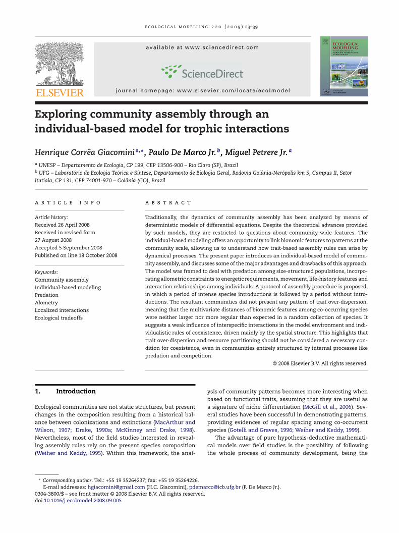
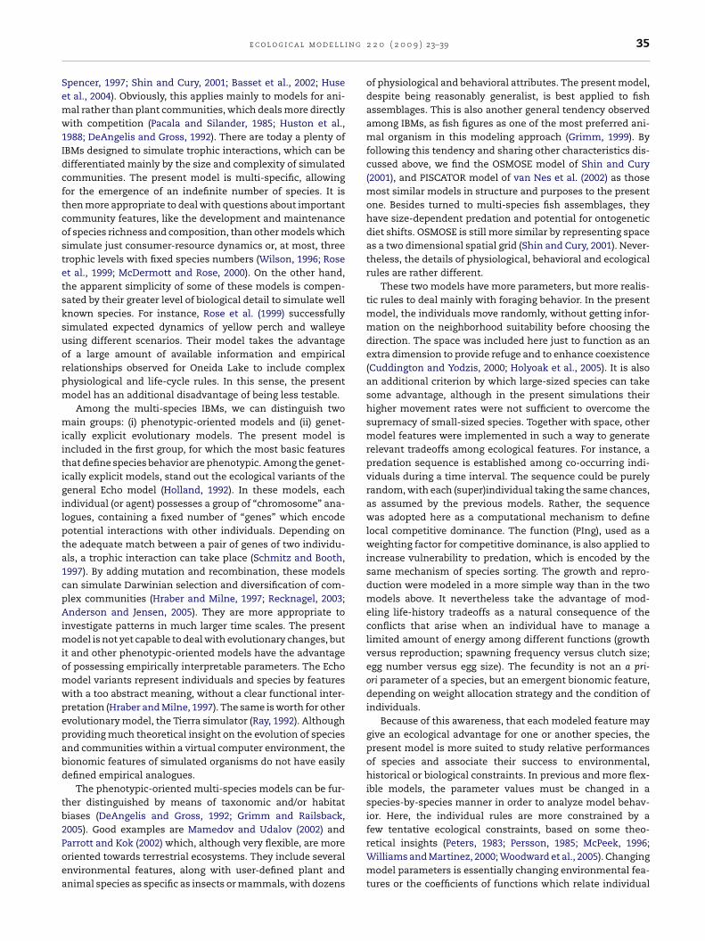
Fig. 1 – Outline of the processes that promote community

e c o l o g i c a l m o d e l l i

.1. Model overview

.1.1. Purposehe objective of the model is to improve understanding aboutow bionomic characteristics of species can be related to eachther when restricting the composition and the structure ofcommunity during its assembly. Fishes are the group of

rganisms for which the rules were referenced, although theodel is sufficiently general to apply to other heterotrophic

roups.

.1.2. State variables and scaless other assembly models, the present model assumes twocales: a local, consisting in a community of co-occurringpecies whose dynamics is modeled explicitly; and a regional,hich includes a pool of immigrant species. In the local scale,

he model comprehends two entities: (i) the environment,hich comprises a rectangular 20 × 20 space grid containingdefined number of basal resources and (ii) the consumers’

ssemblage, whose individuals (or super-individuals) arexplicitly represented. The state of a basal resource, in eachpatial cell, is given by its biomass. The consumer individu-ls are characterized by the following state variables: speciesdentity, age (T), developmental stage (juvenile or adult),lapsed time since the beginning of the reproductive periodtr), spatial position (cell coordinates), weight (W), realizedngestion (Ing) and the number of components (for the casef super-individuals, N).

The individual’s total weight is divided among two vari-bles: the irreversible weight (X) and the reversible weightY) (Claessen et al., 2002). The reversible weight representseserve tissue, like fat or muscles, which can be used whenhe metabolic demands exceed the ingested food. Duringpawning, the offspring comes from the reversible weight. Therreversible weight is constituted by permanent tissue, whichan just grow or stay constant in time. It represents a great pro-ortion of organs like bones, the nervous system and all otherinimum parts necessary to guarantee the vital functions of

he organism.To work with a reasonably great number of individuals, we

sed the super-individual concept, as proposed by Scheffert al. (1995). A super-individual is simply a group of identicalnd co-occurring organisms. It differs from a unitary individ-al just by having a number of components (N) larger than. It is assumed that very similar individuals do not needo be modeled separately, as they do not differ significantlyn their effects upon the environment. Besides, groupingrganisms in super-individuals is analogous to schooling, soommon in fish (Shin and Cury, 2001; Kemelrijk and Kunz,005). In this model, a super-individual is created when eachsuper)female spawns. The young are then followed as a sin-le entity. The number of a super-individual’s components cannly decrease or remain constant. They can be dissociatedfter achieving a size limit of 1 kg (based on the irreversibleeight of each component), and then they start acting sepa-

ately.

The dynamics of the basal resources occur independently

n each cell. The environment is spatially homogeneous:he intrinsic growth rate and the carrying capacity of eachesource do not present differences among spatial cells.

dynamics, during a time interval.

2.1.3. Process overview and schedulingThe time is discreet. For the simulations here presented,we chose the week as the time interval, as a compromisebetween a good time resolution and a reasonable speedfor the simulations. During an interval, the main processesof the internal dynamics happen in the order specified byFig. 1.

Only individuals contained in a same spatial cell caninteract with each other in a same time interval. Dur-ing the execution of the predation module, the spatialcells are processed sequentially, following firstly the spa-tial lines (y dimension) and after the spatial columns(x dimension). For each cell, it is defined the order inwhich the individuals will have access to the consumption(Fig. 1), according to their demands and trophic specialization(see Section 2.5.4).

The life cycle is quite simplified: the newborn individual is

already a juvenile, which can move and feed; its growth, if notprejudiced by competition and/or reproduction, goes along itsentire lifetime; the reproduction is size-dependent, occurringperiodically until death.

l i n g

26 e c o l o g i c a l m o d e l

2.2. Design concepts

2.2.1. EmergenceThe entire dynamics of the consumers populations (fishes)is an emergent result from the behavior and the interac-tions among individuals. The rules are all designed for theindividual, using none population or community level infor-mation, like carrying capacity or species richness, to influenceindividual behavior. Also, the entire trophic structure of com-munities, including number of trophic levels, is an emergentproperty. The trophic level of a species depends on the cir-cumstantial size relationships among their individuals andindividuals of other species.

2.2.2. SensingThe individuals are assumed as capable to distinguish: (i)resource types (including fish) (ii) the size of the items (basalresources or individuals) that can be ingested and be con-tained in the same spatial cell and (iii) the degree of activityof other individuals.

2.2.3. InteractionThe interactions in the model are restricted to predation,which takes place by explicit weight transferring from prey(basal resource or individuals) to an individual predator.

2.2.4. StochasticityIt is included in three processes: (i) during the creation of aspecies; (ii) in initial spatial positioning and during the move-ment of each individual and (iii) in the ordination of predationprocesses.

2.2.5. ObservationAlong each simulation, it stored information about the bio-nomic parameters of species, the permanence time of eachone, the final abundance (number of individuals and biomass)of successful species and the richness of the community alongits development.

2.3. Initialization

At the beginning of assembly process, the basal resources arein their carrying capacity. Whenever a species is introducedin the system, it is constituted by 10 propagules, in identicalcondition:

(X + Y) = WmatWmax;

Y

X= qj

(1)

where X and Y are the irreversible and reversible weights,respectively; Wmax, Wmat and qj are bionomic parameters, thefirst is the maximum weight, the second is the proportion ofthe maximum weight in which the individual becomes adultand the third is the maximum permissible ratio between Yand X for the juvenile. So, the propagules are in great juvenile

condition, but at the beginning of reproductive life. They aredistributed at random in space. Its initial age is zero, althoughthey already have size of an adult. By this way, they have alarger reproductive potential than that for the species they

2 2 0 ( 2 0 0 9 ) 23–39

represent. The age zero was used to avoid some practical dif-ficulties.

2.4. Input

There are no external environmental variables that imposeconditions to the internal dynamics of resources and individ-uals (“input” variables, sensu Grimm et al., 2006). The onlyexternal disturbance consists in the periodic species introduc-tions.

2.5. Submodels

2.5.1. Basal resourcesThe growth of each resource in a spatial cell follows the dis-creet logistic model (Eq. (8), Table 1 ). The susceptibility toconsumption is determined by the “particulate size” of theresource, which represents the range of lengths of the con-stituent particles of the resource (assumed implicitly). The sizedeterminants of resources are the parameters r1 and r2, theinferior size and the superior size, respectively. It was mod-eled 20 basal resources, composing 10 pairs of resources withidentical particulate sizes. The sizes are contiguous amongadjacent pairs of resources, from 0 to 17 cm, following expo-nential increasing of the mean sizes and the range of sizes, insuch a way to create a higher resource concentration at smallersizes in a linear scale (Table 1).

2.5.2. The individual growthThe individual growth in a time interval (�W) is determinedby the difference between the ingested food and the weightloss. The weight loss, given by the power function (Loss = cWd),is fixed for a given size. The realized ingestion (Ing) may notbe the same as the potential ingestion, PIng, specified bythe power function (PIng = aWb), because it also depends onfood availability. It was not used any explicit measure of foodassimilation efficiency. It was considered that the unassim-ilated food is implicitly incorporated by the power functionfor weight loss. In the case of a negative yield, the differ-ence is subtracted from the reversible weight. If the reversibleweight is not enough, the individual dies by starvation. In thecase of a positive yield, it is allocated in different proportionsamong the reversible and irreversible weights, in such a wayto maintain the individual as close as possible to its maximumcondition (qj or qa, if juvenile or adult), according to Eq. (14).

2.5.3. DietAn important concept included in the model is the preda-tion window, which is the range of food sizes susceptible tobe ingested by the individual (Claessen et al., 2002). The infe-rior and superior limits of the predation window are constantproportions of the body length. These proportions are the bio-nomic parameters ı and ε, respectively. The length, calculatedby means of the weight–length relationship L = eWf, is usedinstead of the weight because the ingestion of preys is usuallylimited by their linear dimensions. The difference between ε

and ı give us a relative measure of the diet generality of aspecies.

The diet is also determined by alimentary preferences,imposing the order in which the resources (including fish, as

e c o l o g i c a l m o d e l l i n g 2 2 0 ( 2 0 0 9 ) 23–39 27

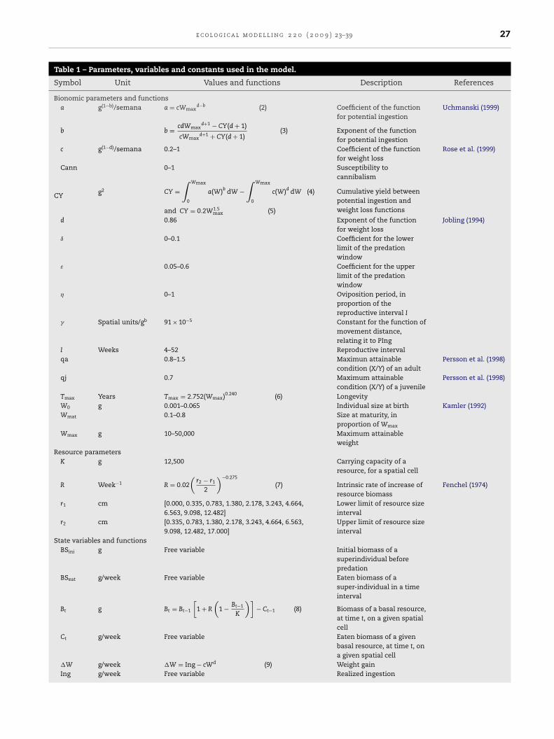
Table 1 – Parameters, variables and constants used in the model.

Symbol Unit Values and functions Description References

Bionomic parameters and functionsa g(1−b)/semana a = cWmax

d−b (2) Coefficient of the functionfor potential ingestion

Uchmanski (1999)

b b = cdWmaxd+1 − CY(d + 1)

cWmaxd+1 + CY(d + 1)

(3) Exponent of the functionfor potential ingestion

c g(1−d)/semana 0.2–1 Coefficient of the functionfor weight loss

Rose et al. (1999)

Cann 0–1 Susceptibility tocannibalism

CY g2 CY =∫ Wmax

0

a(W)b dW −∫ Wmax

0

c(W)d dW (4) Cumulative yield betweenpotential ingestion andweight loss functionsand CY = 0.2W1.5

max (5)d 0.86 Exponent of the function

for weight lossJobling (1994)

ı 0–0.1 Coefficient for the lowerlimit of the predationwindow

ε 0.05–0.6 Coefficient for the upperlimit of the predationwindow

� 0–1 Oviposition period, inproportion of thereproductive interval I

� Spatial units/gb 91 × 10−5 Constant for the function ofmovement distance,relating it to PIng

I Weeks 4–52 Reproductive intervalqa 0.8–1.5 Maximun attainable

condition (X/Y) of an adultPersson et al. (1998)

qj 0.7 Maximum attainablecondition (X/Y) of a juvenile

Persson et al. (1998)

Tmax Years Tmax = 2.752(Wmax)0.240 (6) LongevityW0 g 0.001–0.065 Individual size at birth Kamler (1992)Wmat 0.1–0.8 Size at maturity, in

proportion of Wmax

Wmax g 10–50,000 Maximum attainableweight

Resource parametersK g 12,500 Carrying capacity of a

resource, for a spatial cell

R Week−1 R = 0.02(

r2 − r1

2

)−0.275

(7) Intrinsic rate of increase ofresource biomass

Fenchel (1974)

r1 cm [0.000, 0.335, 0.783, 1.380, 2.178, 3.243, 4.664,6.563, 9.098, 12.482]

Lower limit of resource sizeinterval

r2 cm [0.335, 0.783, 1.380, 2.178, 3.243, 4.664, 6.563,9.098, 12.482, 17.000]

Upper limit of resource sizeinterval

State variables and functionsBSini g Free variable Initial biomass of a

superindividual beforepredation

BSeat g/week Free variable Eaten biomass of asuper-individual in a timeinterval

Bt g Bt = Bt−1

[1 + R

(1 − Bt−1

K

)]− Ct−1 (8) Biomass of a basal resource,

at time t, on a given spatialcell

Ct g/week Free variable Eaten biomass of a givenbasal resource, at time t, ona given spatial cell

�W g/week �W = Ing − cWd (9) Weight gainIng g/week Free variable Realized ingestion

28 e c o l o g i c a l m o d e l l i n g 2 2 0 ( 2 0 0 9 ) 23–39

Table 1 – (Continued )

Symbol Unit Values and functions Description References

� Spatial unit � = � PIng (10) Expected number of spatialcells crossed by anindividual in a week

N Individual N = floor(

Weggs0.5

W0

)for its conception (11) Number of constituents of a

super individualN =floor

(BSini − BSeat

X + Y

)for predation mortality

(12)

N = floor(

IngPIng

)for starvation mortality (13)

pi pi = �W + Y − qX

�W(1 + q)q = qj or qa (14) Proportion of weight gain

allocated to irreversibleweight

PIng g/week PIng = aWb (15) Potential ingestionT Weeks Free variable Age of a (super)individualtr Week Free variable Elapsed time since the

beginning of a reproductiveperiod

W g W = X + Y (16) Weight

Weggs g/week Weggs = Y − qjX

�I − tr(17) Weight used to

reproductionX g Free variable Irreversible weightY g Free variable Reversible weight

ramen “flo

The references are those that supplied information on the referred pavalues are not exactly the same from the original works). The functio

a whole group) are accessed by the consumers during the pre-dation phase. Such preferences are defined randomly and arefixed for each consumer species. Although there is an orderpreferably imposed to the species, the diet must obey the pre-dation window. During the predation sequence, an individualwill change to the second preferential resource only if the firstgoes completely exhausted, and so on.

2.5.4. Predation dynamicsThe competition among individuals is totally asymmetrical.When the resource density is not enough to supply the wholedemand in a spatial cell, it is distributed unevenly among theconsumers, in such a way to supply sequentially the totaldemand of the first (super)individuals, possibly leaving somelast in the sequence without food. It is reasonable to sup-pose that the foraging activity is proportional to the potentialingestion function PIng, as this represents the demand forfood. Following the logic of tradeoffs proposed by the model,another factor used as determinant in the competitiveness isthe degree of “predation efficiency”, or specialization, calcu-lated as the inverse of the diet generality. So, the ratio betweenPIng and generality, PIng/(ε–ı), gives the relative chance of agiven (super)individual to be raffled during the ordination ofthe consumption. After being raffled, the items of its poten-tial diet are ordered according to its preferences. The fishessuitable to be part of the diet are also ordered by draw, withproportional chances to their PIng. This procedure includesan explicit tradeoff between the individual competitiveness

and the susceptibility to predation. To control the cannibal-ism, it was included the parameter Cann, that varies fromzero to one. Before the ordination of potential preys, thisparameter is multiplied to the PIng of co-specifics to give

ters, and also those that help estimating their values (although someor” means rounding to the least integer.

their relative chances of being raffled. The consumer thenfeeds sequentially on the resources, until the (super)individualsatisfies its demand or until the exhaustion of susceptibleresources. A unitary individual partially consumed is con-sidered dead, and all its remaining weight is lost from thesystem. The partial consumption of a super-individual hasthe effect of decreasing the number of their representatives(N), according to Eq. (12). After having consumed and beingupdated, the individual will still be available to be predatedhereafter. If a super-individual consume less than its totaldemand, an asymmetrical competition is established amongtheir representatives, diminishing its number according to Eq.(13). After that whole sequence, a new (super)individual israffled. The procedure is repeated until all (super)individualshave been raffled. If a given resource is completely depletedin a spatial cell, it recolonizes by a standard amountof 1 g.

2.5.5. ReproductionThe individual becomes adult when it reaches a certain pro-portion (Wmat) of its maximum weight (Wmax). Each speciesis characterized by a minimum interval among reproductiveevents (I). Another parameter, �, determines the proportion ofsuch reproductive interval in which spawning occurs, varyingfrom zero to one. The partial amount to be spawned in eachinterval, Weggs, is calculated in such a way that, at the end ofthe reproductive period, the whole content has been emptied(Eq. (17)). All reversible weight that exceeds the expected from

maximum juvenile condition (qj), is available for reproduc-tion. Once adult, the maximum condition increases to qa. Thedifference between qa and qj gives the maximum gonad con-dition, a measure of reproductive investment of the species.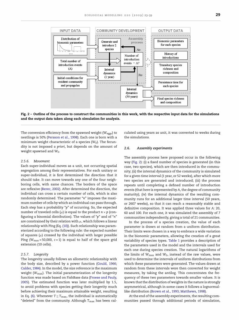

e c o l o g i c a l m o d e l l i n g 2 2 0 ( 2 0 0 9 ) 23–39 29

F in tha s.

Tnmdw

2EsssbairmEnfiareoPe

2TtCwf2tbi“

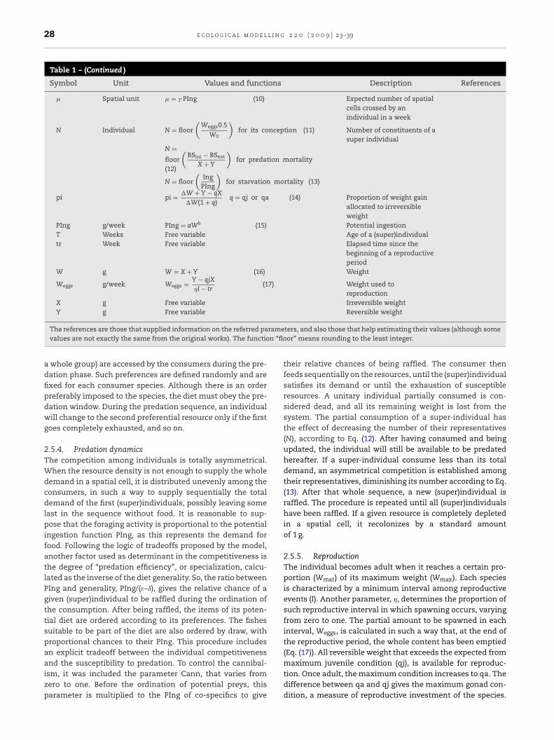
ig. 2 – Outline of the process to construct the communitiesnd the output data taken along each simulation for analysi

he conversion efficiency from the spawned weight (Weggs) toestlings is 50% (Persson et al., 1998). Each one is born with ainimum weight characteristic of a species (W0). The fecun-

ity is not imposed a priori, but depends on the amount ofeight spawned and W0.

.5.6. Movementach super-individual moves as a unit, not occurring spatialegregation among their representatives. For each unitary oruper-individual, it is first determined the direction that ithould take. It can move towards any one of the four neigh-oring cells, with same chances. The borders of the spacere reflexive (Berec, 2002). After determined the direction, thendividual can cross a certain number of cells, which is alsoandomly determined. The parameter “n” imposes the maxi-

um number of cells by which an individual can pass through.ach step has a probability “p” of occurring. So, the expectedumber of traveled cells (�) is equal to the product n × p (con-guring a binomial distribution). The values of “p” and of “n”re constrained by their relation with �, which follows a linearelationship with PIng (Eq. (10)). Such relationship was param-terized according to the following rule: the expected numberf squares (�) crossed by the individual with larger possibleIng (Wmax = 50,000, c = 1) is equal to half of the space gridxtension (10 cells).

.5.7. Longevityhe longevity usually follows an allometric relationship with

he body size, described by a power function (Gould, 1966;alder, 1984). In the model, the size reference is the maximumeight (Wmax). The initial parameterization of the longevity

unction was made based on FishBase data (Froese and Pauly,005). The estimated function was later multiplied by 1.5,

o avoid problems with species getting their longevity muchefore achieving their maximum attainable weight, resulting

n Eq. (6). Whenever T ≥ Tmax, the individual is automaticallydeleted” from the community. Although Tmax has been cal-

is work, with the respective input data for the simulations

culated using years as unit, it was converted to weeks duringthe simulations.

2.6. Assembly experiments

The assembly process here proposed occur in the followingway (Fig. 2): (i) a fixed number of species is generated (in thiscase, two species), which are then introduced in the commu-nity; (ii) the internal dynamics of the community is simulatedfor a given time interval (1 year, or 52 weeks), after which moretwo species are generated and introduced; (iii) the processrepeats until completing a defined number of introductionevents (that here is represented by A, the degree of communitymaturity); (iv) the internal dynamics of the resulting com-munity runs for an additional larger time interval (50 years,or 2607 weeks), so that it can reach a reasonably stable anddefinitive composition. It was applied three values for A: 20,60 and 100. For each one, it was simulated the assembly of 7communities independently, giving a total of 21 communities.

In the process of a species creation, the value of eachparameter is drawn at random from a uniform distribution.Their limits were chosen in a way to embrace a wide variationin the bionomic parameters, allowing the creation of a greatvariability of species types. Table 1 provides a description ofthe parameters used in the model and the intervals used foreach one during species creation. The natural logarithms ofthe limits of Wmax and W0, instead of the raw values, wereused to determine the intervals of uniform distributions fromwhich these parameters were generated. The values drawn atrandom from these intervals were then converted for weightmeasures, by taking the antilog. This concentrates the fre-quency of these two parameters towards smaller values. It isknown that the distribution of weights in the nature is strongly

asymmetrical, although in some cases it follows a lognormal-like distribution (Brown et al., 1993; Matthews, 1998).

At the end of the assembly experiments, the resulting com-munities passed through additional periods of simulation,

l i n g

saturation, but it can just be noticed in the cases with A = 60or 100. After ceasing the invasions, a period of fast richnessdecrease is proceeded, which shows that species immigra-tion was essential to the maintenance of the richness levels

Fig. 3 – Progression of the consumer species richnessduring the assembly processes. For each level of the factorA (total number of introduction events), seven independentprocesses were simulated, whose richness curves are

30 e c o l o g i c a l m o d e l

with the purpose of accessing their degree of persistence. Foreach community, it was done more 27 independent simula-tions, 50 years each, giving a total of 21 × 27 = 567 additionalsimulations. In each simulation, it was used as initial stateexactly the same final state of the previous assembly experi-ment.

2.7. Analysis

To test whether final species richness is affected by the degreeof community maturity (A), it was made a Kruskal–Wallistest. It was not possible to access the formation of somepersistent composition by the same methods used in the tra-ditional models. However, other type of information can beused as criterion: the average permanence time of the com-munity’s constituent species. When a species is introduced,its permanence time is zero by definition. From this point, thepermanence time accompanies the passage of the simulationtime, until that species extinguishes. The average perma-nence time is the arithmetic mean of permanence times of thepresent species in each community, in each moment along asimulation. It can indicate whether the community acquired aresistant formation of species, what can be verified through anull model, in which the extinctions occur in an indiscrim-inate way. The null model here elaborated keeps the samehistory of the number of introductions and extinctions of eachcommunity. For each community history, it was made 1000null model simulations. The trajectories of the 21 communi-ties generated in the assembly experiments were comparedto the 2.5–97.5% percentile region from the totality of values(21,000) generated according to the null model.

To analyze the convergence in bionomic characteristicsof the successful species, it was made a multiple logis-tic regression, having as dependent variable the speciespresence–absence in the final community and as independentvariables the following bionomic characteristics: ln(Wmax), c, ε,�, Wmat, ı, I, qa, Cann and ln(W0). Other parameters had fixedvalues in the simulations (Table 1), so they did not enter in thisanalysis.

To verify if competition-based assembly rules restrictedthe composition of the final communities, and if such rulesare susceptible to be detected by methods commonly used inempirical studies, null models based on the bionomic char-acteristics of the species were tested against observed data(Gotelli and Graves, 1996). A series of combinations of char-acteristics was tested, through two metrics: (i) the averagenearest neighbor distance (ANND) among species in a com-munity and (ii) the standard deviation of the same distances(SDNND) (Travis and Ricklefs, 1983; Gotelli and Graves, 1996).Firstly, all of the bionomic characteristics were standardizedto have average zero and standard deviation 1, providing thema common scaling and equal importance for multivariate dis-tances. The first test involved all of the characteristics withvariation among species (the same 10 used for logistic regres-sion). It was generated a null distribution of ANND and SDNNDfor each species richness (S), in an interval that included all

richness values obtained from assembly experiments. Eachnull distribution was generated by means of 1000 randomdrawing of S species without replacement among all suc-cessful species pertaining to the 21 resulting communities.

2 2 0 ( 2 0 0 9 ) 23–39

The same procedure was repeated for other combinationsof bionomic characteristics: (i) each feature separately; (ii)ln(Wmax), ı, ε, and Cann, which define the diet more directly;(ii) ı, ε, Cann and the logarithm of the length at maturity(calculated from Wmax, Wmat, qj and the weight–length rela-tionship); (iii) just the logarithm of the length at maturity; (iv)ln(Wmax), Wmat, �, I, qa, and ln(W0), which define reproductivestrategies.

3. Results

A total of 215, out of 2305 species, were able to survive to theend of assembly experiments. The mean abundance amongthese successful species, measured at the end of assemblyprocesses, was 1516 individuals (here including juvenile), andthe mean biomass was only 3685 g. The mean biomass ofeach community and the mean number of individuals did notpresent any tendency with respect to species richness (forbiomass: R2 = 0.023, F (1, 19) = 0.284, p = 0.624; for number ofindividuals: R2 = 0.002, F (1, 19) = 0.022, p = 0.884). The predationinteractions among successful consumer species were mainlycannibalistic, representing 98.1% of the individuals’ biomassconsumed during the additional simulations.

3.1. Community development: richness and speciesviability

Fig. 3 depicts the progression of species richness of the con-sumer assemblages along time. There is a visible tendency to

shown overlaid. Two species were added every year in eachassembly, until the point demarcated by the dotted line.After that point, the simulations were run for more 50years.

n g 2 2 0 ( 2 0 0 9 ) 23–39 31

pefiTaa

fpwme

3

Fottomsllccciottla

3o

TtTWwt

cbi

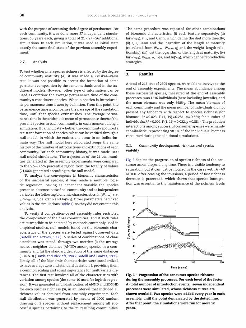
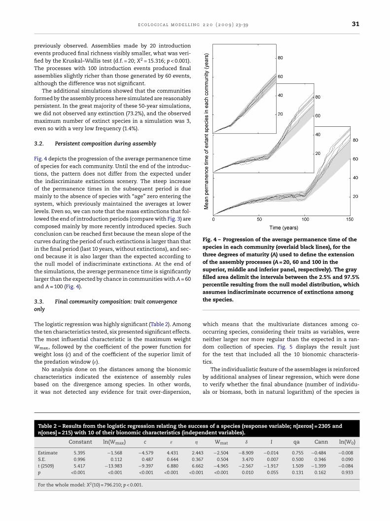
Fig. 4 – Progression of the average permanence time of thespecies in each community (overlaid black lines), for thethree degrees of maturity (A) used to define the extensionof the assembly processes (A = 20, 60 and 100 in thesuperior, middle and inferior panel, respectively). The grayfilled area delimit the intervals between the 2.5% and 97.5%percentile resulting from the null model distribution, which

e c o l o g i c a l m o d e l l i

reviously observed. Assemblies made by 20 introductionvents produced final richness visibly smaller, what was veri-ed by the Kruskal–Wallis test (d.f. = 20; X2 = 15.316; p < 0.001).he processes with 100 introduction events produced finalssemblies slightly richer than those generated by 60 events,lthough the difference was not significant.

The additional simulations showed that the communitiesormed by the assembly process here simulated are reasonablyersistent. In the great majority of these 50-year simulations,e did not observed any extinction (73.2%), and the observedaximum number of extinct species in a simulation was 3,

ven so with a very low frequency (1.4%).

.2. Persistent composition during assembly

ig. 4 depicts the progression of the average permanence timef species for each community. Until the end of the introduc-ions, the pattern does not differ from the expected underhe indiscriminate extinctions scenery. The steep increasef the permanence times in the subsequent period is dueainly to the absence of species with “age” zero entering the

ystem, which previously maintained the averages at lowerevels. Even so, we can note that the mass extinctions that fol-owed the end of introduction periods (compare with Fig. 3) areomposed mainly by more recently introduced species. Suchonclusion can be reached first because the mean slope of theurves during the period of such extinctions is larger than thatn the final period (last 10 years, without extinctions), and sec-nd because it is also larger than the expected according tohe null model of indiscriminate extinctions. At the end ofhe simulations, the average permanence time is significantlyarger than the expected by chance in communities with A = 60nd A = 100 (Fig. 4).

.3. Final community composition: trait convergencenly

he logistic regression was highly significant (Table 2). Amonghe ten characteristics tested, six presented significant effects.he most influential characteristic is the maximum weight

max, followed by the coefficient of the power function foreight loss (c) and of the coefficient of the superior limit of

he predation window (ε).

No analysis done on the distances among the bionomic

haracteristics indicated the existence of assembly rulesased on the divergence among species. In other words,

t was not detected any evidence for trait over-dispersion,

Table 2 – Results from the logistic regression relating the succesn[ones] = 215) with 10 of their bionomic characteristics (indepen

Constant ln(Wmax) c ε �

Estimate 5.395 −1.568 −4.579 4.431 2.443S.E. 0.996 0.112 0.487 0.644 0.367t (2509) 5.417 −13.983 −9.397 6.880 6.662p <0.001 <0.001 <0.001 <0.001 <0.001

For the whole model: X2(10) = 796.210; p < 0.001.

assumes indiscriminate occurrence of extinctions amongthe species.

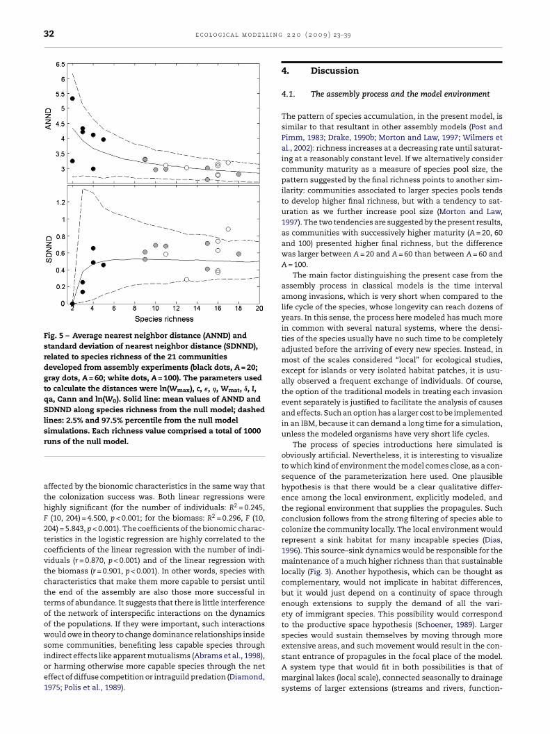
which means that the multivariate distances among co-occurring species, considering their traits as variables, wereneither larger nor more regular than the expected in a ran-dom collection of species. Fig. 5 displays the result justfor the test that included all the 10 bionomic characteris-tics.

The individualistic feature of the assemblages is reinforcedby additional analyses of linear regression, which were doneto verify whether the final abundance (number of individu-als or biomass, both in natural logarithm) of the species is

s of a species (response variable; n[zeros] = 2305 anddent variables).

Wmat ı I qa Cann ln(W0)

−2.504 −8.909 −0.014 0.755 −0.484 −0.0080.504 3.470 0.007 0.500 0.346 0.090

−4.965 −2.567 −1.917 1.509 −1.399 −0.084<0.001 0.010 0.055 0.131 0.162 0.933

32 e c o l o g i c a l m o d e l l i n g

Fig. 5 – Average nearest neighbor distance (ANND) andstandard deviation of nearest neighbor distance (SDNND),related to species richness of the 21 communitiesdeveloped from assembly experiments (black dots, A = 20;gray dots, A = 60; white dots, A = 100). The parameters usedto calculate the distances were ln(Wmax), c, ε, �, Wmat, ı, I,qa, Cann and ln(W0). Solid line: mean values of ANND andSDNND along species richness from the null model; dashedlines: 2.5% and 97.5% percentile from the null modelsimulations. Each richness value comprised a total of 1000

stant entrance of propagules in the focal place of the model.

runs of the null model.

affected by the bionomic characteristics in the same way thatthe colonization success was. Both linear regressions werehighly significant (for the number of individuals: R2 = 0.245,F (10, 204) = 4.500, p < 0.001; for the biomass: R2 = 0.296, F (10,204) = 5.843, p < 0.001). The coefficients of the bionomic charac-teristics in the logistic regression are highly correlated to thecoefficients of the linear regression with the number of indi-viduals (r = 0.870, p < 0.001) and of the linear regression withthe biomass (r = 0.901, p < 0.001). In other words, species withcharacteristics that make them more capable to persist untilthe end of the assembly are also those more successful interms of abundance. It suggests that there is little interferenceof the network of interspecific interactions on the dynamicsof the populations. If they were important, such interactionswould owe in theory to change dominance relationships insidesome communities, benefiting less capable species throughindirect effects like apparent mutualisms (Abrams et al., 1998),

or harming otherwise more capable species through the neteffect of diffuse competition or intraguild predation (Diamond,1975; Polis et al., 1989).

2 2 0 ( 2 0 0 9 ) 23–39

4. Discussion

4.1. The assembly process and the model environment

The pattern of species accumulation, in the present model, issimilar to that resultant in other assembly models (Post andPimm, 1983; Drake, 1990b; Morton and Law, 1997; Wilmers etal., 2002): richness increases at a decreasing rate until saturat-ing at a reasonably constant level. If we alternatively considercommunity maturity as a measure of species pool size, thepattern suggested by the final richness points to another sim-ilarity: communities associated to larger species pools tendsto develop higher final richness, but with a tendency to sat-uration as we further increase pool size (Morton and Law,1997). The two tendencies are suggested by the present results,as communities with successively higher maturity (A = 20, 60and 100) presented higher final richness, but the differencewas larger between A = 20 and A = 60 than between A = 60 andA = 100.

The main factor distinguishing the present case from theassembly process in classical models is the time intervalamong invasions, which is very short when compared to thelife cycle of the species, whose longevity can reach dozens ofyears. In this sense, the process here modeled has much morein common with several natural systems, where the densi-ties of the species usually have no such time to be completelyadjusted before the arriving of every new species. Instead, inmost of the scales considered “local” for ecological studies,except for islands or very isolated habitat patches, it is usu-ally observed a frequent exchange of individuals. Of course,the option of the traditional models in treating each invasionevent separately is justified to facilitate the analysis of causesand effects. Such an option has a larger cost to be implementedin an IBM, because it can demand a long time for a simulation,unless the modeled organisms have very short life cycles.

The process of species introductions here simulated isobviously artificial. Nevertheless, it is interesting to visualizeto which kind of environment the model comes close, as a con-sequence of the parameterization here used. One plausiblehypothesis is that there would be a clear qualitative differ-ence among the local environment, explicitly modeled, andthe regional environment that supplies the propagules. Suchconclusion follows from the strong filtering of species able tocolonize the community locally. The local environment wouldrepresent a sink habitat for many incapable species (Dias,1996). This source–sink dynamics would be responsible for themaintenance of a much higher richness than that sustainablelocally (Fig. 3). Another hypothesis, which can be thought ascomplementary, would not implicate in habitat differences,but it would just depend on a continuity of space throughenough extensions to supply the demand of all the vari-ety of immigrant species. This possibility would correspondto the productive space hypothesis (Schoener, 1989). Largerspecies would sustain themselves by moving through moreextensive areas, and such movement would result in the con-

A system type that would fit in both possibilities is that ofmarginal lakes (local scale), connected seasonally to drainagesystems of larger extensions (streams and rivers, function-

n g

i1kttrrwTe

stAsrwIreldea

4

Arsp(twtsttmpnrisEccwowrea1ttrcat

e c o l o g i c a l m o d e l l i

ng as propagule suppliers) (Lowe-McConnell, 1987; Wooton,992). Many freshwater systems present flood pulses of thisind (De Angelis et al., 2005; Bayley, 1995; Benke et al., 2000). Inhe model, in analogy to the natural system described above,he end of the immigration period could represent the inter-uption of the connection between the lake and the river. Ineal situations, this can happen by changing the flood regime,hich is usually observed as an effect of dams (Baxter, 1977).he curves of Fig. 3 illustrate well what would be the expectedffect on the local richness in such a situation.

The convergence of the bionomic characteristics favoredpecies with little energetic requirements, generalists (rela-ively to their size) and with larger reproductive allocation.ll of this, allied to the low observed biomass of consumers,uggests that the total productivity of the modeled local iselatively low. Another factor is the mobility of individuals,hich indirectly defines the extension of the modeled space.

ndividuals with little mobility may starve by overexploitingesources in their local spatial cells if these are not productivenough. The allometric function relating the body size to theocomotion capacity was not parameterized according to realata. It does not mean that the parameterization was inher-ntly incorrect, but just that we did not have an initial forecastbout what extension the modeled space exactly represented.

.2. Community maturity

s expected, the community maturity influenced the finalichness of species positively, what follows predictions ofimpler models (Post and Pimm, 1983; Pimm, 1991). Two com-lementary factors may be employed to explain this effect:

i) a sampling factor, of individualistic feature and (ii) a holis-ic factor, of adjustment among species. The sampling effect,hich does not depend necessarily on interspecific interac-

ions, refers to the fact that the species are created by atochastic Monte Carlo procedure, and that just a proportion ofhem are capable to establish in the modeled environment. Byhis way, the number of species minimally capable to colonize

ay be thought as a binomially distributed variable, whosearameter “p” is the proportion above mentioned and “n” is theumber of attempts, in other words, of species generated atandom. The expected value of the number of capable speciess then n × p. Consequently, increasing the number of createdpecies lead to increasing mean number of capable species.ven so, increasing the maturity also increases the chance ofreating minimally adjusted species. In this case of holisticonstraint, each species can be visualized as a puzzle piece,hich depends not only on being capable individually to col-nize the model environment, but it must “fit” appropriatelyith other present pieces (Drake, 1990a). Most of the assembly

ules investigated in ecological works have a holistic character,mphasizing the importance of interspecific interactions (Foxnd Brown, 1993; Gotelli and Graves, 1996; Weiher and Keddy,999; Gotelli and McCabe, 2002). It is interesting to note thathe use of Lotka–Volterra models follows an intrinsically holis-ic approach, once the purpose of its application is to study the

elationships among species and most of their parameters areomprised by interaction coefficients. However, both holisticnd individualistic factors are important to explain the selec-ion of species during the formation of a community and the

2 2 0 ( 2 0 0 9 ) 23–39 33

resulting richness. It is their relative importance which canvary from system to system (Gleason, 1926; Clements, 1916;Matthews, 1998; Brown et al., 2001). In the environment heremodeled, the evidences point to a more individualistic controlof communities.

4.3. The individualistic feature of coexistence

The progression of the permanence time (Fig. 4) suggests thatthe structuring of the communities only becomes apparentafter interrupting the introductions. This is in agreement withthe general theory of assembly (Luh and Pimm, 1993) and alsowith predictions of Lotka–Volterra models (Lockwood et al.,1997). The interesting here is that, immediately after ceas-ing the introductions, the curves of the permanence time arealready steeper than the expected from the null model. Itsuggests that there was a community formation “ready” toorganize, even coming immediately from a period of frequentintroductions, which in a first analysis was not different toa null model. However, such a propensity do not necessarilyimplicate that holistic properties are involved in the selectionof the assemblages. An individualistic explanation could per-fectly fit the observed pattern. If the most capable species arealso the oldest, on average, it would suffice. Indeed, there wasa significant negative correlation between the permanencetime and the maximum weight (ln[Wmax]) during the period ofintroductions (r = −0.314, p < 0.001). But, if there was a “ready”group of more capable (smaller) and older species, how couldthe null model of random extinctions explain the permanencedata during the whole period of introductions?

The fact that the extinctions happen indiscriminatelyregarding the permanence time just implies that, during theintroductions period, the more persistent species were notsynchronized in time, preventing the formation of a cohesivegroup. They were introduced and extinguished in a discon-nected way. What promoted the extinction of these specieswere not necessarily other more capable species. A constantentrance of species, even if less capable, could generate a neg-ative effect strong enough (Lockwood et al., 1997).

Some complementary evidences in the Section 3 of thiswork point to an individualistic control in the final formationand maintenance of the communities: (i) the mean abun-dance does not decrease with richness; (ii) species with largerchance of colonizing become also the most abundant in thefinal communities; (iii) the cannibalism prevailed among thepredation interactions of the successful species and (iv) it wasnot observed any divergence pattern among the co-occurringspecies. Anyway, those species are capable to coexist in theirlocal communities, in most of cases, for more than 100 years(taking into account the additional simulations). Althoughsome analyses in the literature defend a criterion of infinitetime to define the conditions for stable coexistence (Chessonand Huntly, 1997), such criterion seems without meaning in aworld of constant changes, and being known that extinctionsare inevitable in a limit of time so long as infinite (McKinneyand Drake, 1998). To the view of any nature observer, a 100

years interval seems sufficiently long to be necessary invok-ing coexistence mechanisms, even for organisms like thosehere modeled, whose maximum longevity is about 12 years(considering just the successful species).

l i n g

34 e c o l o g i c a l m o d e l

The coexistence can be sustained by means of equalizingand stabilizing mechanisms (Chesson, 2000). The equaliz-ing mechanisms result from tradeoffs among several speciesfunctions and requirements in the environment, beingresponsible for equaling the fitness of competing species andso delaying the course of competitive exclusions. Stabilizingmechanisms, on the other hand, act in a frequency depen-dent way, ensuring that the effects of relatively more abundantspecies rely mainly on themselves (Chesson, 2000; Adler etal., 2007). Having in mind that the resulting species of thepresent model possess different characteristics and quality,which is translated in a predictable way in their abundances,some stabilizing factor should contribute to keep their coexis-tence. The first option, niche partitioning, was not detected asa plausible factor by the analyses of species divergence in thiswork. Other mechanisms as the storage effect should not con-tribute, as they depend on temporal or spatial heterogeneityin the conditions to work (Chesson, 1985). The same is worthfor the occurrence of disturbances (Huston, 1979). In theory,sustained fluctuations in the levels of the resources, evenwhen caused internally by the consumer-resource dynamics,could maintain a great diversity of species if these possessnonlinear responses to resources with different nonlinearities(Armstrong and McGehee, 1980). However, great fluctuationswere not verified in the resources. Besides, the functionalresponse of the species can be considered of the type 1 (Begonet al., 1996), and therefore linear, as the resource uptake by anindividual is not affected by resource density, except when theconsumers’ demand exceeds the availability. Another mecha-nism, the intraguild predation, theoretically can facilitate thecoexistence when the species that prevail as predators arealso the worst competitors (Polis and Holt, 1992). However,the great predominance of cannibalism does not support thishypothesis. In the case of the present model, the most prob-able mechanism for explaining the coexistence concerns thespatial division and the localized character of the interactions.

The successful species have small body size when com-pared to the initial universe of possibilities. Besides, due tothe parameterization particularities, they possess a very lowlocomotion capacity. To best illustrate this, the largest of thesuccessful species (Wmax = 452.32 g, Wmat = 0.60), immediatelyafter reaching maturity (271.39 g), can move for at the mostone spatial cell during a time interval, even so with a prob-ability of only 3%. Individuals confined in a spatial cell canquickly deplete the resources there available if it is not produc-tive enough. The low mobility also explains the prevalence ofcannibalism, as the individuals were born in the same spatialcell of their parent. Even competitively superior species are notcapable to disseminate entirely in the environment, becausetheir “superiority” will be restricted to one or a few spatialunits. As a result, it creates spatial refuges for less capablespecies.

The spatial aggregation can stabilize the dynamics ofpredator–prey or parasitoid–host systems. For instance,Hassell and May (1974) have already shown that the aggre-gation of predators (parasitoids) in places of larger densities

of the prey (hosts) stabilize the system and facilitate the coex-istence of both. The spatial division associated to a limitedcapacity of dispersion produces a similar effect, increasing thechances of coexistence among metapopulations of competi-

2 2 0 ( 2 0 0 9 ) 23–39

tors (Hanski, 1981). Cuddington and Yodzis (2000) argue thatthe increasing stability of spatial consumer-resource dynam-ics can simply be explained by the decrease in the meanefficiency of the predator. They showed that an identical effectcan happen by diminishing the interaction coefficient in aLotka–Volterra model of predation, without needing spatialdivision. In other words, in systems with dispersion limita-tion, the interspecific interactions tend to be weaker. The sameshould be worth for the system modeled in the present work.The isolation promoted by the spatial division and the lowmovement rates turns intraspecific interactions stronger thanthe interspecific interactions. Indeed, we can state that this isthe only universal condition for species coexistence (Chesson,2000).

The prevalence of weak interspecific interactions seems tobe the rule in ecological communities (McCann et al., 1998;Berlow, 1999; Dunne, 2005). The destabilizing effect of stronginteractions was already recognized since May (1973). Some ofthe best studied empirical food webs demonstrate an asym-metrical pattern of distribution of the intensity of interactions,in which the great majority of the observed links has rela-tively low values, while a few have high values (de Ruiter etal., 1995; McCann et al., 1998). The asymmetrical pattern hasbeen resulted also from some assembly models (Caldarelli etal., 1998). Kokkoris et al. (1999) demonstrated that the meancoefficient of interaction decreases as competitive communi-ties governed by Lotka–Volterra equations were assembled.Once strong interactions tend to be destabilizing, it is quiteplausible that the communities can grow, on average, just byaccumulating weaker interactions. Although the interactionintensities have not been measured in the present work, veryprobably they followed the same pattern, decreasing along thetime. Larger species, with larger energetic demand and withlarger locomotion capacity, certainly contributed to the for-mation of links with stronger intensity. Maybe this constitutesan additional and more holistic reason for such species beingexcluded from the final communities.

4.4. Comparison with other similar IBMs

The present model follows some general tendencies ofindividual-based models designed to study communitydynamics. First, as an IBM, it incorporates more biologicalcomplexities to rule species interactions than classical statevariable models, like Lotka–Volterra (Grimm, 1999). On theother hand, the IBM approach is less generalist, applying tosituations more specific than those characterizing classicalmodels. There are many other similar tradeoffs concerningthe usefulness of these two approaches, and they have beenalready discussed elsewhere in reviews about IBM advan-tages and disadvantages (DeAngelis and Gross, 1992; Judson,1994; Grimm, 1999; Lomnicki, 1999; Railsback, 2001; Grimmand Railsback, 2005; Giacomini, 2007). As the comparisonbetween the present model and the several Lotka–Volterra-liketrophic models will inevitably return to the so much discusseddichotomy “IBM” versus “Classical”, we will not deal with it

here.

Another tendency observed among community IBMs is thegreat importance attributed to trophic interactions among thefactors structuring communities (Schmitz and Booth, 1997;

n g

Semw1Idcftcostetsksuorpm

miitigilpta1cpAimiomwpepabd

tb2Poea

e c o l o g i c a l m o d e l l i

pencer, 1997; Shin and Cury, 2001; Basset et al., 2002; Huset al., 2004). Obviously, this applies mainly to models for ani-al rather than plant communities, which deals more directlyith competition (Pacala and Silander, 1985; Huston et al.,

988; DeAngelis and Gross, 1992). There are today a plenty ofBMs designed to simulate trophic interactions, which can beifferentiated mainly by the size and complexity of simulatedommunities. The present model is multi-specific, allowingor the emergence of an indefinite number of species. It ishen more appropriate to deal with questions about importantommunity features, like the development and maintenancef species richness and composition, than other models whichimulate just consumer-resource dynamics or, at most, threerophic levels with fixed species numbers (Wilson, 1996; Roset al., 1999; McDermott and Rose, 2000). On the other hand,he apparent simplicity of some of these models is compen-ated by their greater level of biological detail to simulate wellnown species. For instance, Rose et al. (1999) successfullyimulated expected dynamics of yellow perch and walleyesing different scenarios. Their model takes the advantagef a large amount of available information and empiricalelationships observed for Oneida Lake to include complexhysiological and life-cycle rules. In this sense, the presentodel has an additional disadvantage of being less testable.Among the multi-species IBMs, we can distinguish two

ain groups: (i) phenotypic-oriented models and (ii) genet-cally explicit evolutionary models. The present model isncluded in the first group, for which the most basic featureshat define species behavior are phenotypic. Among the genet-cally explicit models, stand out the ecological variants of theeneral Echo model (Holland, 1992). In these models, eachndividual (or agent) possesses a group of “chromosome” ana-ogues, containing a fixed number of “genes” which encodeotential interactions with other individuals. Depending onhe adequate match between a pair of genes of two individu-ls, a trophic interaction can take place (Schmitz and Booth,997). By adding mutation and recombination, these modelsan simulate Darwinian selection and diversification of com-lex communities (Hraber and Milne, 1997; Recknagel, 2003;nderson and Jensen, 2005). They are more appropriate to

nvestigate patterns in much larger time scales. The presentodel is not yet capable to deal with evolutionary changes, but

t and other phenotypic-oriented models have the advantagef possessing empirically interpretable parameters. The Echoodel variants represent individuals and species by featuresith a too abstract meaning, without a clear functional inter-retation (Hraber and Milne, 1997). The same is worth for othervolutionary model, the Tierra simulator (Ray, 1992). Althoughroviding much theoretical insight on the evolution of speciesnd communities within a virtual computer environment, theionomic features of simulated organisms do not have easilyefined empirical analogues.

The phenotypic-oriented multi-species models can be fur-her distinguished by means of taxonomic and/or habitatiases (DeAngelis and Gross, 1992; Grimm and Railsback,005). Good examples are Mamedov and Udalov (2002) and

arrott and Kok (2002) which, although very flexible, are moreriented towards terrestrial ecosystems. They include severalnvironmental features, along with user-defined plant andnimal species as specific as insects or mammals, with dozens

2 2 0 ( 2 0 0 9 ) 23–39 35

of physiological and behavioral attributes. The present model,despite being reasonably generalist, is best applied to fishassemblages. This is also another general tendency observedamong IBMs, as fish figures as one of the most preferred ani-mal organism in this modeling approach (Grimm, 1999). Byfollowing this tendency and sharing other characteristics dis-cussed above, we find the OSMOSE model of Shin and Cury(2001), and PISCATOR model of van Nes et al. (2002) as thosemost similar models in structure and purposes to the presentone. Besides turned to multi-species fish assemblages, theyhave size-dependent predation and potential for ontogeneticdiet shifts. OSMOSE is still more similar by representing spaceas a two dimensional spatial grid (Shin and Cury, 2001). Never-theless, the details of physiological, behavioral and ecologicalrules are rather different.

These two models have more parameters, but more realis-tic rules to deal mainly with foraging behavior. In the presentmodel, the individuals move randomly, without getting infor-mation on the neighborhood suitability before choosing thedirection. The space was included here just to function as anextra dimension to provide refuge and to enhance coexistence(Cuddington and Yodzis, 2000; Holyoak et al., 2005). It is alsoan additional criterion by which large-sized species can takesome advantage, although in the present simulations theirhigher movement rates were not sufficient to overcome thesupremacy of small-sized species. Together with space, othermodel features were implemented in such a way to generaterelevant tradeoffs among ecological features. For instance, apredation sequence is established among co-occurring indi-viduals during a time interval. The sequence could be purelyrandom, with each (super)individual taking the same chances,as assumed by the previous models. Rather, the sequencewas adopted here as a computational mechanism to definelocal competitive dominance. The function (PIng), used as aweighting factor for competitive dominance, is also applied toincrease vulnerability to predation, which is encoded by thesame mechanism of species sorting. The growth and repro-duction were modeled in a more simple way than in the twomodels above. It nevertheless take the advantage of mod-eling life-history tradeoffs as a natural consequence of theconflicts that arise when an individual have to manage alimited amount of energy among different functions (growthversus reproduction; spawning frequency versus clutch size;egg number versus egg size). The fecundity is not an a pri-ori parameter of a species, but an emergent bionomic feature,depending on weight allocation strategy and the condition ofindividuals.

Because of this awareness, that each modeled feature maygive an ecological advantage for one or another species, thepresent model is more suited to study relative performancesof species and associate their success to environmental,historical or biological constraints. In previous and more flex-ible models, the parameter values must be changed in aspecies-by-species manner in order to analyze model behav-ior. Here, the individual rules are more constrained by afew tentative ecological constraints, based on some theo-

retical insights (Peters, 1983; Persson, 1985; McPeek, 1996;Williams and Martinez, 2000; Woodward et al., 2005). Changingmodel parameters is essentially changing environmental fea-tures or the coefficients of functions which relate individual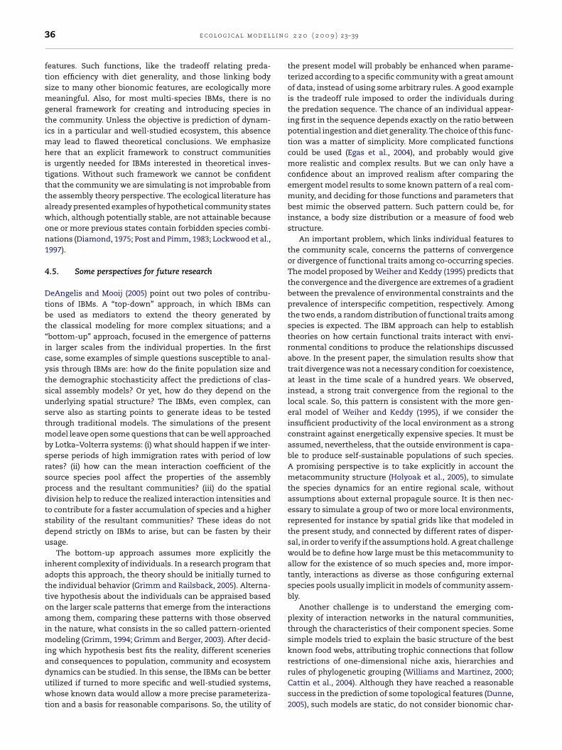

l i n g

36 e c o l o g i c a l m o d e l

features. Such functions, like the tradeoff relating preda-tion efficiency with diet generality, and those linking bodysize to many other bionomic features, are ecologically moremeaningful. Also, for most multi-species IBMs, there is nogeneral framework for creating and introducing species inthe community. Unless the objective is prediction of dynam-ics in a particular and well-studied ecosystem, this absencemay lead to flawed theoretical conclusions. We emphasizehere that an explicit framework to construct communitiesis urgently needed for IBMs interested in theoretical inves-tigations. Without such framework we cannot be confidentthat the community we are simulating is not improbable fromthe assembly theory perspective. The ecological literature hasalready presented examples of hypothetical community stateswhich, although potentially stable, are not attainable becauseone or more previous states contain forbidden species combi-nations (Diamond, 1975; Post and Pimm, 1983; Lockwood et al.,1997).

4.5. Some perspectives for future research

DeAngelis and Mooij (2005) point out two poles of contribu-tions of IBMs. A “top-down” approach, in which IBMs canbe used as mediators to extend the theory generated bythe classical modeling for more complex situations; and a“bottom-up” approach, focused in the emergence of patternsin larger scales from the individual properties. In the firstcase, some examples of simple questions susceptible to anal-ysis through IBMs are: how do the finite population size andthe demographic stochasticity affect the predictions of clas-sical assembly models? Or yet, how do they depend on theunderlying spatial structure? The IBMs, even complex, canserve also as starting points to generate ideas to be testedthrough traditional models. The simulations of the presentmodel leave open some questions that can be well approachedby Lotka–Volterra systems: (i) what should happen if we inter-sperse periods of high immigration rates with period of lowrates? (ii) how can the mean interaction coefficient of thesource species pool affect the properties of the assemblyprocess and the resultant communities? (iii) do the spatialdivision help to reduce the realized interaction intensities andto contribute for a faster accumulation of species and a higherstability of the resultant communities? These ideas do notdepend strictly on IBMs to arise, but can be fasten by theirusage.

The bottom-up approach assumes more explicitly theinherent complexity of individuals. In a research program thatadopts this approach, the theory should be initially turned tothe individual behavior (Grimm and Railsback, 2005). Alterna-tive hypothesis about the individuals can be appraised basedon the larger scale patterns that emerge from the interactionsamong them, comparing these patterns with those observedin the nature, what consists in the so called pattern-orientedmodeling (Grimm, 1994; Grimm and Berger, 2003). After decid-ing which hypothesis best fits the reality, different sceneriesand consequences to population, community and ecosystem

dynamics can be studied. In this sense, the IBMs can be betterutilized if turned to more specific and well-studied systems,whose known data would allow a more precise parameteriza-tion and a basis for reasonable comparisons. So, the utility of

2 2 0 ( 2 0 0 9 ) 23–39

the present model will probably be enhanced when parame-terized according to a specific community with a great amountof data, instead of using some arbitrary rules. A good exampleis the tradeoff rule imposed to order the individuals duringthe predation sequence. The chance of an individual appear-ing first in the sequence depends exactly on the ratio betweenpotential ingestion and diet generality. The choice of this func-tion was a matter of simplicity. More complicated functionscould be used (Egas et al., 2004), and probably would givemore realistic and complex results. But we can only have aconfidence about an improved realism after comparing theemergent model results to some known pattern of a real com-munity, and deciding for those functions and parameters thatbest mimic the observed pattern. Such pattern could be, forinstance, a body size distribution or a measure of food webstructure.

An important problem, which links individual features tothe community scale, concerns the patterns of convergenceor divergence of functional traits among co-occurring species.The model proposed by Weiher and Keddy (1995) predicts thatthe convergence and the divergence are extremes of a gradientbetween the prevalence of environmental constraints and theprevalence of interspecific competition, respectively. Amongthe two ends, a random distribution of functional traits amongspecies is expected. The IBM approach can help to establishtheories on how certain functional traits interact with envi-ronmental conditions to produce the relationships discussedabove. In the present paper, the simulation results show thattrait divergence was not a necessary condition for coexistence,at least in the time scale of a hundred years. We observed,instead, a strong trait convergence from the regional to thelocal scale. So, this pattern is consistent with the more gen-eral model of Weiher and Keddy (1995), if we consider theinsufficient productivity of the local environment as a strongconstraint against energetically expensive species. It must beassumed, nevertheless, that the outside environment is capa-ble to produce self-sustainable populations of such species.A promising perspective is to take explicitly in account themetacommunity structure (Holyoak et al., 2005), to simulatethe species dynamics for an entire regional scale, withoutassumptions about external propagule source. It is then nec-essary to simulate a group of two or more local environments,represented for instance by spatial grids like that modeled inthe present study, and connected by different rates of disper-sal, in order to verify if the assumptions hold. A great challengewould be to define how large must be this metacommunity toallow for the existence of so much species and, more impor-tantly, interactions as diverse as those configuring externalspecies pools usually implicit in models of community assem-bly.

Another challenge is to understand the emerging com-plexity of interaction networks in the natural communities,through the characteristics of their component species. Somesimple models tried to explain the basic structure of the bestknown food webs, attributing trophic connections that followrestrictions of one-dimensional niche axis, hierarchies and

rules of phylogenetic grouping (Williams and Martinez, 2000;Cattin et al., 2004). Although they have reached a reasonablesuccess in the prediction of some topological features (Dunne,2005), such models are static, do not consider bionomic char-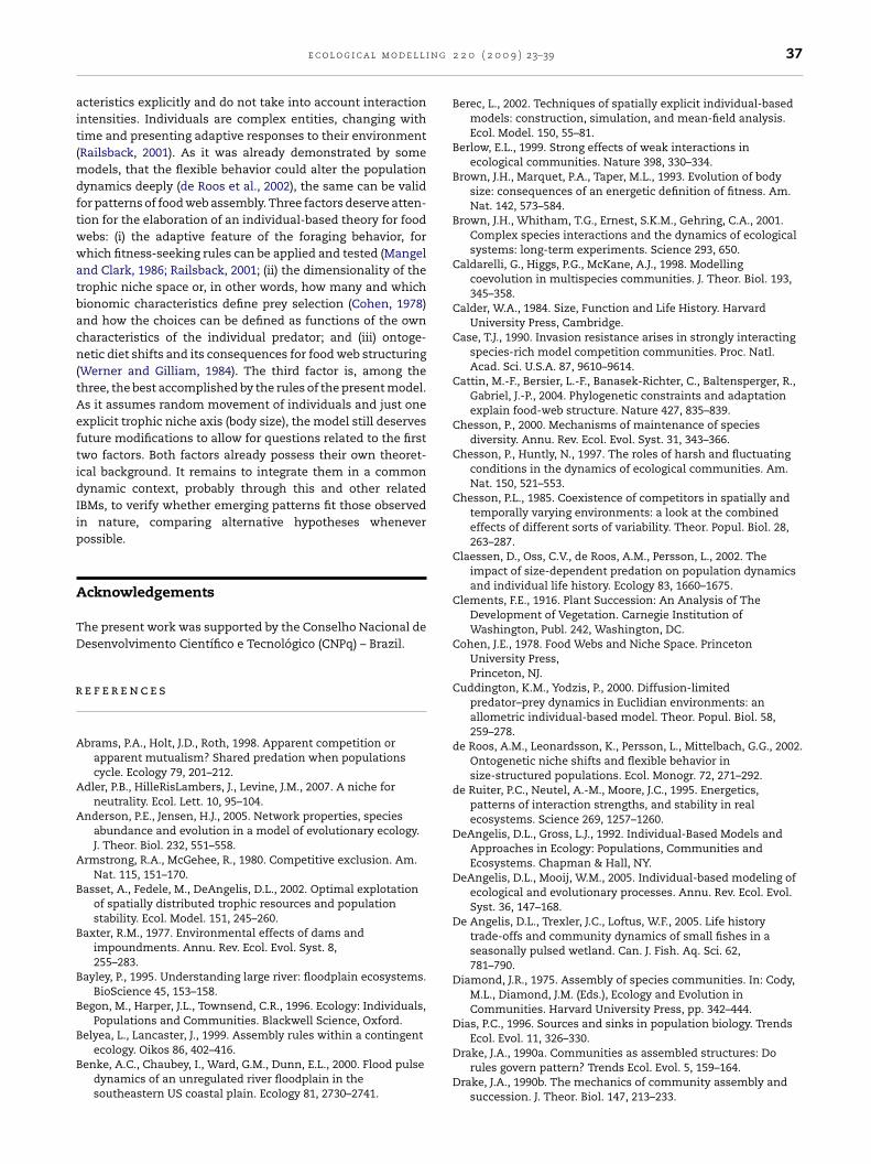

n g

ait(mdftwwatbacn(tAeftidIip

A

TD

r

A

A

A

A

B

B

B

B

B

B

e c o l o g i c a l m o d e l l i

cteristics explicitly and do not take into account interactionntensities. Individuals are complex entities, changing withime and presenting adaptive responses to their environmentRailsback, 2001). As it was already demonstrated by some

odels, that the flexible behavior could alter the populationynamics deeply (de Roos et al., 2002), the same can be validor patterns of food web assembly. Three factors deserve atten-ion for the elaboration of an individual-based theory for foodebs: (i) the adaptive feature of the foraging behavior, forhich fitness-seeking rules can be applied and tested (Mangel

nd Clark, 1986; Railsback, 2001; (ii) the dimensionality of therophic niche space or, in other words, how many and whichionomic characteristics define prey selection (Cohen, 1978)nd how the choices can be defined as functions of the ownharacteristics of the individual predator; and (iii) ontoge-etic diet shifts and its consequences for food web structuring

Werner and Gilliam, 1984). The third factor is, among thehree, the best accomplished by the rules of the present model.s it assumes random movement of individuals and just onexplicit trophic niche axis (body size), the model still deservesuture modifications to allow for questions related to the firstwo factors. Both factors already possess their own theoret-cal background. It remains to integrate them in a commonynamic context, probably through this and other relatedBMs, to verify whether emerging patterns fit those observedn nature, comparing alternative hypotheses wheneverossible.

cknowledgements

he present work was supported by the Conselho Nacional deesenvolvimento Científico e Tecnológico (CNPq) – Brazil.

e f e r e n c e s

brams, P.A., Holt, J.D., Roth, 1998. Apparent competition orapparent mutualism? Shared predation when populationscycle. Ecology 79, 201–212.

dler, P.B., HilleRisLambers, J., Levine, J.M., 2007. A niche forneutrality. Ecol. Lett. 10, 95–104.

nderson, P.E., Jensen, H.J., 2005. Network properties, speciesabundance and evolution in a model of evolutionary ecology.J. Theor. Biol. 232, 551–558.

rmstrong, R.A., McGehee, R., 1980. Competitive exclusion. Am.Nat. 115, 151–170.

asset, A., Fedele, M., DeAngelis, D.L., 2002. Optimal explotationof spatially distributed trophic resources and populationstability. Ecol. Model. 151, 245–260.

axter, R.M., 1977. Environmental effects of dams andimpoundments. Annu. Rev. Ecol. Evol. Syst. 8,255–283.

ayley, P., 1995. Understanding large river: floodplain ecosystems.BioScience 45, 153–158.

egon, M., Harper, J.L., Townsend, C.R., 1996. Ecology: Individuals,Populations and Communities. Blackwell Science, Oxford.

elyea, L., Lancaster, J., 1999. Assembly rules within a contingentecology. Oikos 86, 402–416.

enke, A.C., Chaubey, I., Ward, G.M., Dunn, E.L., 2000. Flood pulsedynamics of an unregulated river floodplain in thesoutheastern US coastal plain. Ecology 81, 2730–2741.

2 2 0 ( 2 0 0 9 ) 23–39 37

Berec, L., 2002. Techniques of spatially explicit individual-basedmodels: construction, simulation, and mean-field analysis.Ecol. Model. 150, 55–81.

Berlow, E.L., 1999. Strong effects of weak interactions inecological communities. Nature 398, 330–334.

Brown, J.H., Marquet, P.A., Taper, M.L., 1993. Evolution of bodysize: consequences of an energetic definition of fitness. Am.Nat. 142, 573–584.

Brown, J.H., Whitham, T.G., Ernest, S.K.M., Gehring, C.A., 2001.Complex species interactions and the dynamics of ecologicalsystems: long-term experiments. Science 293, 650.

Caldarelli, G., Higgs, P.G., McKane, A.J., 1998. Modellingcoevolution in multispecies communities. J. Theor. Biol. 193,345–358.

Calder, W.A., 1984. Size, Function and Life History. HarvardUniversity Press, Cambridge.

Case, T.J., 1990. Invasion resistance arises in strongly interactingspecies-rich model competition communities. Proc. Natl.Acad. Sci. U.S.A. 87, 9610–9614.

Cattin, M.-F., Bersier, L.-F., Banasek-Richter, C., Baltensperger, R.,Gabriel, J.-P., 2004. Phylogenetic constraints and adaptationexplain food-web structure. Nature 427, 835–839.

Chesson, P., 2000. Mechanisms of maintenance of speciesdiversity. Annu. Rev. Ecol. Evol. Syst. 31, 343–366.

Chesson, P., Huntly, N., 1997. The roles of harsh and fluctuatingconditions in the dynamics of ecological communities. Am.Nat. 150, 521–553.

Chesson, P.L., 1985. Coexistence of competitors in spatially andtemporally varying environments: a look at the combinedeffects of different sorts of variability. Theor. Popul. Biol. 28,263–287.

Claessen, D., Oss, C.V., de Roos, A.M., Persson, L., 2002. Theimpact of size-dependent predation on population dynamicsand individual life history. Ecology 83, 1660–1675.

Clements, F.E., 1916. Plant Succession: An Analysis of TheDevelopment of Vegetation. Carnegie Institution ofWashington, Publ. 242, Washington, DC.

Cohen, J.E., 1978. Food Webs and Niche Space. PrincetonUniversity Press,Princeton, NJ.

Cuddington, K.M., Yodzis, P., 2000. Diffusion-limitedpredator–prey dynamics in Euclidian environments: anallometric individual-based model. Theor. Popul. Biol. 58,259–278.

de Roos, A.M., Leonardsson, K., Persson, L., Mittelbach, G.G., 2002.Ontogenetic niche shifts and flexible behavior insize-structured populations. Ecol. Monogr. 72, 271–292.

de Ruiter, P.C., Neutel, A.-M., Moore, J.C., 1995. Energetics,patterns of interaction strengths, and stability in realecosystems. Science 269, 1257–1260.

DeAngelis, D.L., Gross, L.J., 1992. Individual-Based Models andApproaches in Ecology: Populations, Communities andEcosystems. Chapman & Hall, NY.

DeAngelis, D.L., Mooij, W.M., 2005. Individual-based modeling ofecological and evolutionary processes. Annu. Rev. Ecol. Evol.Syst. 36, 147–168.

De Angelis, D.L., Trexler, J.C., Loftus, W.F., 2005. Life historytrade-offs and community dynamics of small fishes in aseasonally pulsed wetland. Can. J. Fish. Aq. Sci. 62,781–790.

Diamond, J.R., 1975. Assembly of species communities. In: Cody,M.L., Diamond, J.M. (Eds.), Ecology and Evolution inCommunities. Harvard University Press, pp. 342–444.

Dias, P.C., 1996. Sources and sinks in population biology. TrendsEcol. Evol. 11, 326–330.

Drake, J.A., 1990a. Communities as assembled structures: Dorules govern pattern? Trends Ecol. Evol. 5, 159–164.

Drake, J.A., 1990b. The mechanics of community assembly andsuccession. J. Theor. Biol. 147, 213–233.

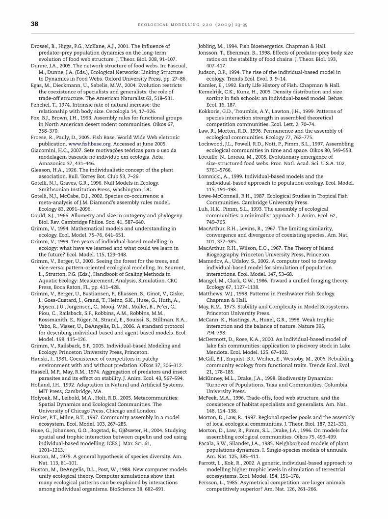
l i n g

38 e c o l o g i c a l m o d e l

Drossel, B., Higgs, P.G., McKane, A.J., 2001. The influence ofpredator–prey population dynamics on the long-termevolution of food web structure. J. Theor. Biol. 208, 91–107.

Dunne, J.A., 2005. The network structure of food webs. In: Pascual,M., Dunne, J.A. (Eds.), Ecological Networks: Linking Structureto Dynamics in Food Webs. Oxford University Press, pp. 27–86.

Egas, M., Dieckmann, U., Sabelis, M.W., 2004. Evolution restrictsthe coexistence of specialists and generalists: the role oftrade-off structure. The American Naturalist 63, 518–531.

Fenchel, T., 1974. Intrinsic rate of natural increase: therelationship with body size. Oecologia 14, 17–326.

Fox, B.J., Brown, J.H., 1993. Assembly rules for functional groupsin North American desert rodent communities. Oikos 67,358–370.

Froese, R., Pauly, D., 2005. Fish Base. World Wide Web eletronicpublication. www.fishbase.org. Accessed at June 2005.

Giacomini, H.C., 2007. Sete motivacões teóricas para o uso damodelagem baseada no indivíduo em ecologia. ActaAmazonica 37, 431–446.

Gleason, H.A., 1926. The individualistic concept of the plantassociation. Bull. Torrey Bot. Club 53, 7–26.

Gotelli, N.J., Graves, G.R., 1996. Null Models in Ecology.Smithsonian Institution Press, Washington, DC.

Gotelli, N.J., McCabe, D.J., 2002. Species co-occurrence: ameta-analysis of J.M. Diamond’s assembly rules model.Ecology 83, 2091–2096.

Gould, S.J., 1966. Allometry and size in ontogeny and phylogeny.Biol. Rev. Cambridge Philos. Soc. 41, 587–640.

Grimm, V., 1994. Mathematical models and understanding inecology. Ecol. Model. 75–76, 641–651.

Grimm, V., 1999. Ten years of individual-based modelling inecology: what have we learned and what could we learn inthe future? Ecol. Model. 115, 129–148.

Grimm, V., Berger, U., 2003. Seeing the forest for the trees, andvice-versa: pattern-oriented ecological modeling. In: Seuront,L., Strutton, P.G. (Eds.), Handbook of Scaling Methods inAquatic Ecology: Measurement, Analysis, Simulation. CRCPress, Boca Raton, FL, pp. 411–428.

Grimm, V., Berger, U., Bastiansen, F., Eliassen, S., Ginot, V., Giske,J., Goss-Custard, J., Grand, T., Heinz, S.K., Huse, G., Huth, A.,Jepsen, J.U., Jorgensen, C., Mooij, W.M., Müller, B., Pe’er, G.,Piou, C., Railsback, S.F., Robbins, A.M., Robbins, M.M.,Rossmanith, E., Rüger, N., Strand, E., Souissi, S., Stillman, R.A.,Vabo, R., Visser, U., DeAngelis, D.L., 2006. A standard protocolfor describing individual-based and agent-based models. Ecol.Model. 198, 115–126.

Grimm, V., Railsback, S.F., 2005. Individual-based Modeling andEcology. Princeton University Press, Princeton.

Hanski, I., 1981. Coexistence of competitors in patchyenvironment with and without predation. Oikos 37, 306–312.

Hassell, M.P., May, R.M., 1974. Aggregation of predators and insectparasites and its effect on stability. J. Anim. Ecol. 43, 567–594.

Holland, J.H., 1992. Adaptation in Natural and Artificial Systems.MIT Press, Cambridge, MA.

Holyoak, M., Leibold, M.A., Holt, R.D., 2005. Metacommunities:Spatial Dynamics and Ecological Communities. TheUniversity of Chicago Press, Chicago and London.

Hraber, P.T., Milne, B.T., 1997. Community assembly in a modelecosystem. Ecol. Model. 103, 267–285.

Huse, G., Johansen, G.O., Bogstad, B., GjØsæter, H., 2004. Studyingspatial and trophic interaction between capelin and cod usingindividual-based modelling. ICES J. Mar. Sci. 61,1201–1213.

Huston, M., 1979. A general hypothesis of species diversity. Am.Nat. 113, 81–101.

Huston, M., DeAngelis, D.L., Post, W., 1988. New computer modelsunify ecological theory. Computer simulations show thatmany ecological patterns can be explained by interactionsamong individual organisms. BioScience 38, 682–691.

2 2 0 ( 2 0 0 9 ) 23–39

Jobling, M., 1994. Fish Bioenergetics. Chapman & Hall.Jonsson, T., Ebenman, B., 1998. Effects of predator–prey body size

ratios on the stability of food chains. J. Theor. Biol. 193,407–417.

Judson, O.P., 1994. The rise of the individual-based model inecology. Trends Ecol. Evol. 9, 9–14.

Kamler, E., 1992. Early Life History of Fish. Chapman & Hall.Kemelrijk, C.K., Kunz, H., 2005. Density distribution and size

sorting in fish schools: an individual-based model. Behav.Ecol. 16, 187.

Kokkoris, G.D., Troumbis, A.Y., Lawton, J.H., 1999. Patterns ofspecies interaction strength in assembled theoreticalcompetition communities. Ecol. Lett. 2, 70–74.

Law, R., Morton, R.D., 1996. Permanence and the assembly ofecological communities. Ecology 77, 762–775.

Lockwood, J.L., Powell, R.D., Nott, P., Pimm, S.L., 1997. Assemblingecological communities in time and space. Oikos 80, 549–553.

Loeuille, N., Loreau, M., 2005. Evolutionary emergence ofsize-structured food webs. Proc. Natl. Acad. Sci. U.S.A. 102,5761–5766.

Lomnicki, A., 1999. Individual-based models and theindividual-based approach to population ecology. Ecol. Model.115, 191–198.

Lowe-McConnell, R.H., 1987. Ecological Studies in Tropical FishCommunities. Cambridge University Press.

Luh, H.K., Pimm, S.L., 1993. The assembly of ecologicalcommunities: a minimalist approach. J. Anim. Ecol. 62,749–765.

MacArthur, R.H., Levins, R., 1967. The limiting similarity,convergence and divergence of coexisting species. Am. Nat.101, 377–385.

MacArthur, R.H., Wilson, E.O., 1967. The Theory of IslandBiogeography. Princeton University Press, Princeton.

Mamedov, A., Udalov, S., 2002. A computer tool to developindividual-based model for simulation of populationinteractions. Ecol. Model. 147, 53–68.

Mangel, M., Clark, C.W., 1986. Toward a unified foraging theory.Ecology 67, 1127–1138.

Matthews, W.J., 1998. Patterns in Freshwater Fish Ecology.Chapman & Hall.

May, R.M., 1973. Stability and Complexity in Model Ecosystems.Princeton University Press.

McCann, K., Hastings, A., Huxel, G.R., 1998. Weak trophicinteraction and the balance of nature. Nature 395,794–798.

McDermott, D., Rose, K.A., 2000. An individual-based model oflake fish communities: application to piscivory stock in LakeMendota. Ecol. Model. 125, 67–102.

McGill, B.J., Enquist, B.J., Weiher, E., Westoby, M., 2006. Rebuildingcommunity ecology from functional traits. Trends Ecol. Evol.21, 178–185.

McKinney, M.L., Drake, J.A., 1998. Biodiversity Dynamics:Turnover of Populations, Taxa and Communities. ColumbiaUniversity Press.

McPeek, M.A., 1996. Trade-offs, food web structure, and thecoexistence of habitat specialists and generalists. Am. Nat.148, 124–138.

Morton, D., Law, R., 1997. Regional species pools and the assemblyof local ecological communities. J. Theor. Biol. 187, 321–331.

Morton, D., Law, R., Pimm, S.L., Drake, J.A., 1996. On models forassembling ecological communities. Oikos 75, 493–499.

Pacala, S.W., Silander, J.A., 1985. Neighborhood models of plantpopulations dynamics. I. Single-species models of annuals.Am. Nat. 125, 385–411.

Parrott, L., Kok, R., 2002. A generic, individual-based approach to

modelling higher trophic levels in simulation of terrestrialecossystems. Ecol. Model. 154, 151–178.

Persson, L., 1985. Asymetrical competition: are larger animalscompetitively superior? Am. Nat. 126, 261–266.

n g

P

P

P

P

P

P

R

R

R

R

S

S

S

e c o l o g i c a l m o d e l l i

ersson, L., Leonardsson, K., de Roos, A.M., Gyllenberg, M.,Christensen, B., 1998. Ontogenetic scaling of foraging ratesand the dynamics of a size-structured consumer-resourcemodel. Theor. Popul. Biol. 54, 270–293.

eters, R.H., 1983. The Ecological Implications of Body Size.Cambridge University Press, Cambridge.

imm, S.L., 1991. The Balance of Nature: Ecological Issues in theConservation of Species and Communities. University ofChicago Press, Chicago, IL.

olis, G.A., Holt, R., 1992. Intraguild predation: the dynamics ofcomplex tropic interactions. Trends Ecol. Evol. 7, 151–154.

olis, G.A., Myers, C.A., Holt, R.D., 1989. The ecology andevolution of intraguild predation—potential competitors thateat each other. Annu. Rev. Ecol. Evol. Syst. 20, 297–330.

ost, W.M., Pimm, S.L., 1983. Community assembly and food webstability. Math. Biosci. 64, 169–192.

ailsback, S.F., 2001. Concepts from complex adaptive systems asa framework for individual-based modelling. Ecol. Model. 139,47–62.

ay, T.S. 1992. Evolution, ecology and optimization of digitalorganisms. Santa Fe Institute working paper 92-08-042.http://www.romanpoet.org/223/Ray.tierra.pdf.

ecknagel, F., 2003. Simulation of aquatic food web and speciesinteractions by adaptive agents embodied with evolutionarycomputation: a conceptual framework. Ecol. Model. 170,291–302.

ose, K.A., Rutherford, E.S., McDermot, D.S., Forney, J.L., Mills,E.L., 1999. Individual-based model of yellow perch andwalleye populations in Oneida Lake. Ecol. Monogr. 69,127–154.

cheffer, M., Baveco, J.M., DeAngelis, D.L., Rose, K.A., van Nes,E.H., 1995. Super-individuals a simple solution for modellinglarge populations on an individual basis. Ecol. Model. 80,161–170.

chmitz, O.J., Booth, G., 1997. Modelling food web complexity: the

consequences of individual-based, spatially explicitbehavioural ecology on trophic interactions. Evol. Ecol. 11,379–398.

choener, T.W., 1989. Food webs from the small to the large.Ecology 70, 1559–1589.

2 2 0 ( 2 0 0 9 ) 23–39 39

Shin, Y.J., Cury, P., 2001. Exploring fish community dynamicsthrough size-dependent trophic interactions using aspatialized individual-based model. Aquat. Living Res. 14,65–80.

Spencer, M., 1997. The effects of habitat size and energy on foodweb structure: an individual-based cellular automata model.Ecol. Model. 94, 299–316.

Travis, J., Ricklefs, R.E., 1983. A morphological comparison ofisland and mainland assemblages of neotropical birds. Oikos41, 434–441.

Uchmanski, J., 1999. What promotes persistence of a singlepopulation: an individual-based model. Ecol. Model. 115,227–241.

Uchmanski, J., Grimm, V., 1996. Individual-based modelling inEcology: what makes the difference? Trends Ecol. Evol. 11,437–441.

van Nes, E.H., Lammens, E.H.R.R., Scheffer, M., 2002. PISCATOR,an individual-based model to analyze the dynamics of lakefish communities. Ecol. Model. 152, 261–278.

Weiher, E., Keddy, P.A., 1995. Assembly rules, null models, andtrait dispersion: new questions from old patterns. Oikos 74,159–164.

Weiher, E., Keddy, P.A., 1999. Ecological Assembly Rules:Perspectives, Advances, Retreats. Cambridge University Press,Cambridge.

Werner, E.E., Gilliam, J.F., 1984. The ontogenetic niche and speciesinteractions in size-structured populations. Annu. Rev. Ecol.Evol. Syst. 15, 393–425.

Williams, R.J., Martinez, N.D., 2000. Simple rules yield complexfood webs. Nature 404, 180–183.

Wilmers, C.C., Sinha, S., Brede, M., 2002. Examining the effects ofspecies richness on community stability: an assembly modelapproach. Oikos 99, 363–376.

Wilson, W.G., 1996. Lotka’s game in predator–prey theory: linkingpopulations to individuals. Theor. Popul. Biol. 50, 368–393.

Woodward, G., Ebenman, B., Emmerson, M.C., Montoya, J.M.,Olesen, J.M., Valido, A., Warren, P.H., 2005. Body size inecological networks. Trends Ecol. Evol. 20,402–409.

Wooton, R.J., 1992. Fish Ecology. Blackie, New York.