Experimental demonstration of fiber Bragg grating strain sensors for structural vibration control
Upload
khangminh22Category
view
1download
0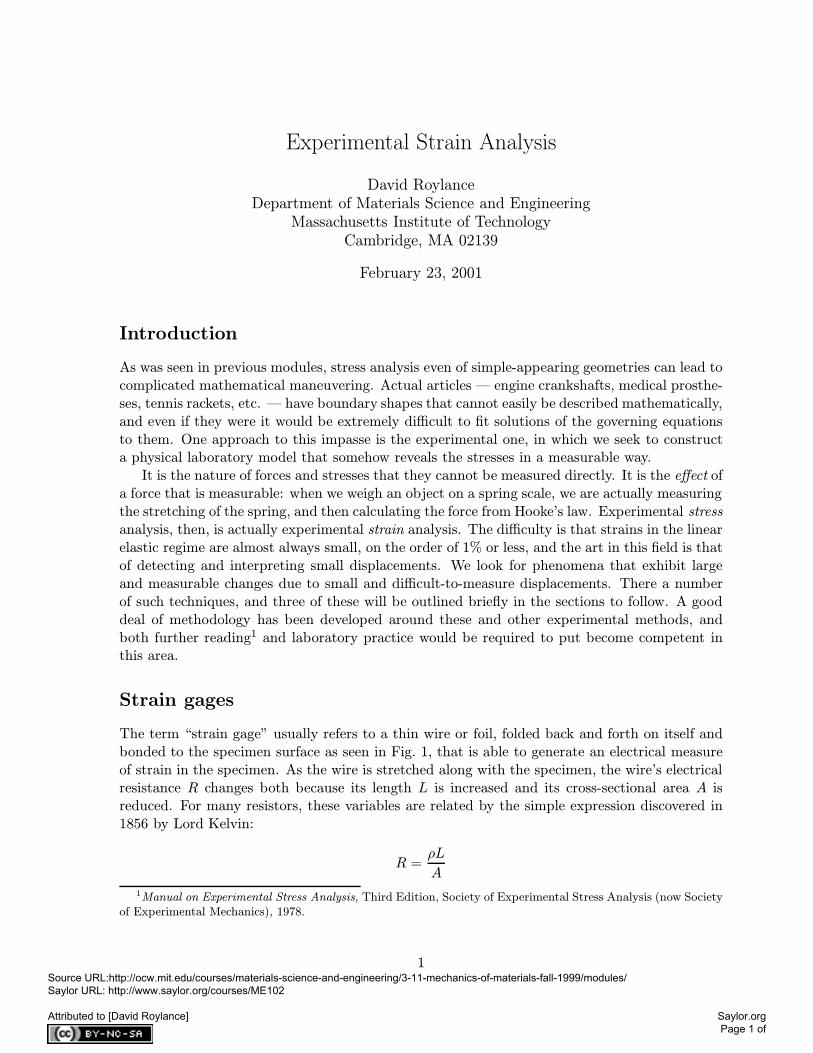
Experimental Strain Analysis
David RoylanceDepartment of Materials Science and Engineering
Massachusetts Institute of TechnologyCambridge, MA 02139
February 23, 2001
Introduction
As was seen in previous modules, stress analysis even of simple-appearing geometries can lead tocomplicated mathematical maneuvering. Actual articles — engine crankshafts, medical prosthe-ses, tennis rackets, etc. — have boundary shapes that cannot easily be described mathematically,and even if they were it would be extremely difficult to fit solutions of the governing equationsto them. One approach to this impasse is the experimental one, in which we seek to constructa physical laboratory model that somehow reveals the stresses in a measurable way.It is the nature of forces and stresses that they cannot be measured directly. It is the effect of
a force that is measurable: when we weigh an object on a spring scale, we are actually measuringthe stretching of the spring, and then calculating the force from Hooke’s law. Experimental stressanalysis, then, is actually experimental strain analysis. The difficulty is that strains in the linearelastic regime are almost always small, on the order of 1% or less, and the art in this field is thatof detecting and interpreting small displacements. We look for phenomena that exhibit largeand measurable changes due to small and difficult-to-measure displacements. There a numberof such techniques, and three of these will be outlined briefly in the sections to follow. A gooddeal of methodology has been developed around these and other experimental methods, andboth further reading1 and laboratory practice would be required to put become competent inthis area.
Strain gages
The term “strain gage” usually refers to a thin wire or foil, folded back and forth on itself andbonded to the specimen surface as seen in Fig. 1, that is able to generate an electrical measureof strain in the specimen. As the wire is stretched along with the specimen, the wire’s electricalresistance R changes both because its length L is increased and its cross-sectional area A isreduced. For many resistors, these variables are related by the simple expression discovered in1856 by Lord Kelvin:
R =ρL
A
1Manual on Experimental Stress Analysis, Third Edition, Society of Experimental Stress Analysis (now Societyof Experimental Mechanics), 1978.
1Source URL:http://ocw.mit.edu/courses/materials-science-and-engineering/3-11-mechanics-of-materials-fall-1999/modules/ Saylor URL: http://www.saylor.org/courses/ME102 Attributed to [David Roylance]
Saylor.org Page 1 of
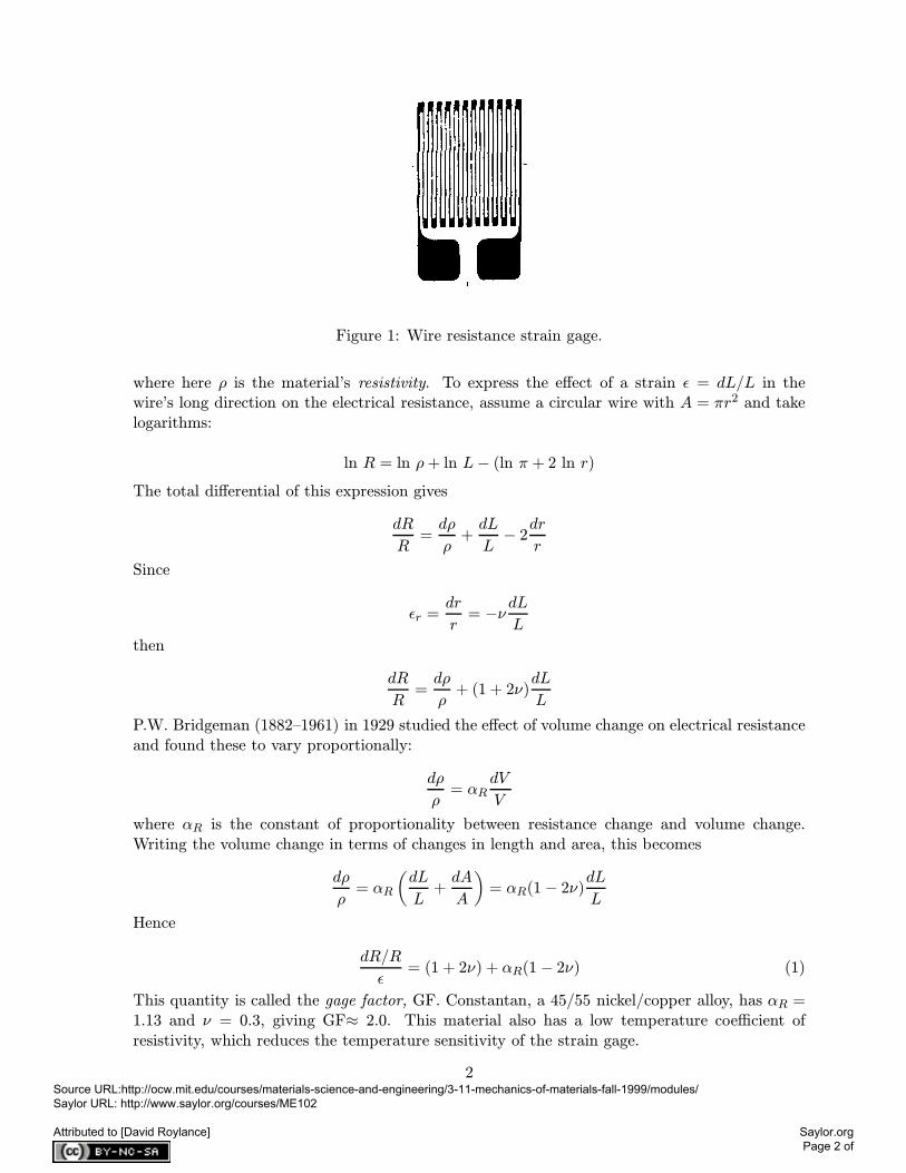
Figure 1: Wire resistance strain gage.
where here ρ is the material’s resistivity. To express the effect of a strain ε = dL/L in thewire’s long direction on the electrical resistance, assume a circular wire with A = πr2 and takelogarithms:
ln R = ln ρ+ ln L− (ln π + 2 ln r)
The total differential of this expression gives
dR
R=dρ
ρ+dL
L− 2dr
r
Since
εr =dr
r= −ν
dL
L
then
dR
R=dρ
ρ+ (1 + 2ν)
dL
L
P.W. Bridgeman (1882–1961) in 1929 studied the effect of volume change on electrical resistanceand found these to vary proportionally:
dρ
ρ= αR
dV
V
where αR is the constant of proportionality between resistance change and volume change.Writing the volume change in terms of changes in length and area, this becomes
dρ
ρ= αR
(dL
L+dA
A
)= αR(1− 2ν)
dL
L
Hence
dR/R
ε= (1 + 2ν) + αR(1 − 2ν) (1)
This quantity is called the gage factor, GF. Constantan, a 45/55 nickel/copper alloy, has αR =1.13 and ν = 0.3, giving GF≈ 2.0. This material also has a low temperature coefficient ofresistivity, which reduces the temperature sensitivity of the strain gage.
2Source URL:http://ocw.mit.edu/courses/materials-science-and-engineering/3-11-mechanics-of-materials-fall-1999/modules/ Saylor URL: http://www.saylor.org/courses/ME102 Attributed to [David Roylance]
Saylor.org Page 2 of

Figure 2: Wheatstone bridge circuit for strain gages.
A change in resistance of only 2%, which would be generated by a gage with GF = 2 at 1%strain, would not be noticeable on a simple ohmmeter. For this reason strain gages are almostalways connected to a Wheatstone-bridge circuit as seen in Fig. 2. The circuit can be adjustedby means of the variable resistance R2 to produce a zero output voltage Vout before strain isapplied to the gage. Typically the gage resistance is approximately 350Ω and the excitationvoltage is near 10V. When the gage resistance is changed by strain, the bridge is unbalancedand a voltage appears on the output according to the relation
VoutVin=∆R
2R0
where R0 is the nominal resistance of the four bridge elements. The output voltage is easilymeasured because it is a deviation from zero rather than being a relatively small change su-perimposed on a much larger quantity; it can thus be amplified to suit the needs of the dataacquisition system.Temperature compensation can be achieved by making a bridge element on the opposite side
of the bridge from the active gage, say R3, an inactive gage that is placed near the active gagebut not bonded to the specimen. Resistance changes in the active gage due to temperature willthen be offset be an equal resistance change in the other arm of the bridge.
Figure 3: Cancellation of bending effects.
3Source URL:http://ocw.mit.edu/courses/materials-science-and-engineering/3-11-mechanics-of-materials-fall-1999/modules/ Saylor URL: http://www.saylor.org/courses/ME102 Attributed to [David Roylance]
Saylor.org Page 3 of
It is often difficult to mount a tensile specimen in the testing machine without inadvertentlyapplying bending in addition to tensile loads. If a single gage were applied to the convex-outward side of the specimen, its reading would be erroneously high. Similarly, a gage placed onthe concave-inward or compressive-tending side would read low. These bending errors can beeliminated by using an active gage on each side of the specimen as shown in Fig. 3 and wiringthem on the same side of the Wheatstone bridge, e.g. R1 and R4. The tensile component ofbending on one side of the specimen is accompanied by an equal but compressive component onthe other side, and these will generate equal but opposite resistance changes in R1 and R4. Theeffect of bending will therefore cancel, and the gage combination will measure only the tensilestrain (with doubled sensitivity, since both R1 and R4 are active).
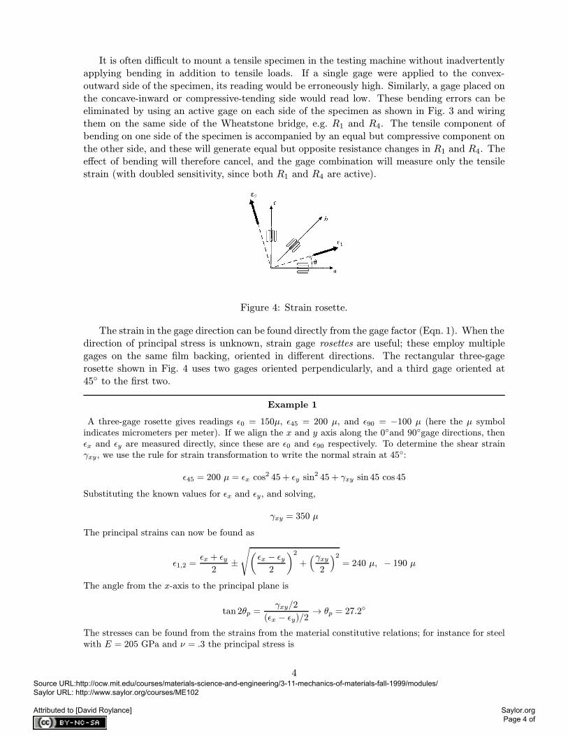
Figure 4: Strain rosette.
The strain in the gage direction can be found directly from the gage factor (Eqn. 1). When thedirection of principal stress is unknown, strain gage rosettes are useful; these employ multiplegages on the same film backing, oriented in different directions. The rectangular three-gagerosette shown in Fig. 4 uses two gages oriented perpendicularly, and a third gage oriented at45 to the first two.
Example 1
A three-gage rosette gives readings ε0 = 150µ, ε45 = 200 µ, and ε90 = −100 µ (here the µ symbolindicates micrometers per meter). If we align the x and y axis along the 0and 90gage directions, thenεx and εy are measured directly, since these are ε0 and ε90 respectively. To determine the shear strainγxy, we use the rule for strain transformation to write the normal strain at 45
:
ε45 = 200 µ = εx cos2 45 + εy sin
2 45 + γxy sin 45 cos 45
Substituting the known values for εx and εy, and solving,
γxy = 350 µ
The principal strains can now be found as
ε1,2 =εx + εy2
±
√(εx − εy2
)2+(γxy2
)2= 240 µ, − 190 µ
The angle from the x-axis to the principal plane is
tan 2θp =γxy/2
(εx − εy)/2→ θp = 27.2
The stresses can be found from the strains from the material constitutive relations; for instance for steelwith E = 205 GPa and ν = .3 the principal stress is
4Source URL:http://ocw.mit.edu/courses/materials-science-and-engineering/3-11-mechanics-of-materials-fall-1999/modules/ Saylor URL: http://www.saylor.org/courses/ME102 Attributed to [David Roylance]
Saylor.org Page 4 of

σ1 =E
1− ν2(ε1 + νε2) = 41.2 MPa
For the specific case of a 0-45-90 rosette, the orientation of the principal strain axis can begiven directly by2
tan 2θ =2εb − εa − εcεa − εc
(2)
and the principal strains are
ε1,2 =εa + εc2
±
√(εa − εb)2 + (εb − εc)2
2(3)
Graphical solutions based on Mohr’s circles are also useful for reducing gage output data.Strain gages are used very extensively, and critical structures such as aircraft may be in-
strumented with hundreds of gages during testing. Each gage must be bonded carefully to thestructure, and connected by its two leads to the signal conditioning unit that includes the excita-tion voltage source and the Wheatstone bridge. This can obviously be a major instrumentationchore, with computer-aided data acquisition and reduction a practical necessity.
Photoelasticity
Wire-resistance strain gages are probably the principal device used in experimental stress anal-ysis today, but they have the disadvantage of monitoring strain only at a single location. Pho-toelasticity and moire methods, to be outlined in the following sections, are more complicatedin concept and application but have the ability to provide full-field displays of the strain distri-bution. The intuitive insight from these displays can be so valuable that it may be unnecessaryto convert them to numerical values, although the conversion can be done if desired.
Figure 5: Light propagation.
Photoelasticity employs a property of many transparent polymers and inorganic glasses calledbirefringence. To explain this phenomenon, recall the definition of refractive index, n, which isthe ratio of the speed of light v in the medium to that in vacuum c:
n =v
c(4)
2M. Hetenyi, ed., Handbook of Experimental Stress Analysis, Wiley, New York, 1950.
5Source URL:http://ocw.mit.edu/courses/materials-science-and-engineering/3-11-mechanics-of-materials-fall-1999/modules/ Saylor URL: http://www.saylor.org/courses/ME102 Attributed to [David Roylance]
Saylor.org Page 5 of
As the light beam travels in space (see Fig. 5), its electric field vector E oscillates up and downat an angular frequency ω in a fixed plane, termed the plane of polarization of the beam. (Thewavelength of the light is λ = 2πc/ω.) A birefringent material is one in which the refractiveindex depends on the orientation of plane of polarization, and magnitude of the birefringence isthe difference in indices:
∆n = n⊥ − n‖
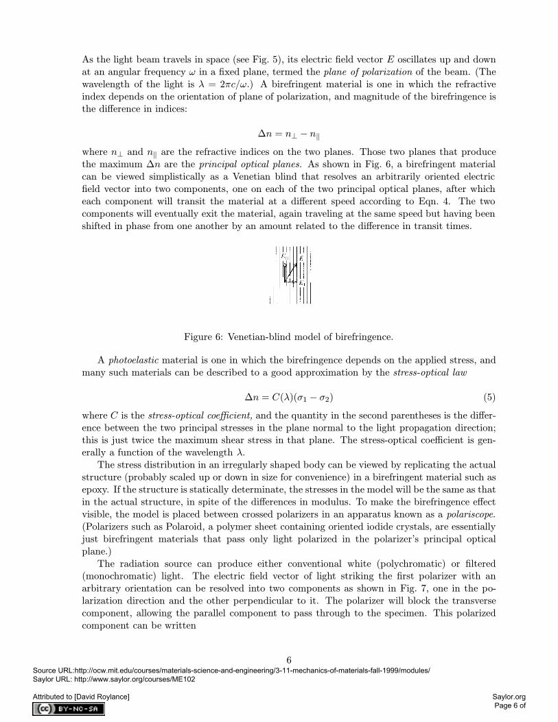
where n⊥ and n‖ are the refractive indices on the two planes. Those two planes that producethe maximum ∆n are the principal optical planes. As shown in Fig. 6, a birefringent materialcan be viewed simplistically as a Venetian blind that resolves an arbitrarily oriented electricfield vector into two components, one on each of the two principal optical planes, after whicheach component will transit the material at a different speed according to Eqn. 4. The twocomponents will eventually exit the material, again traveling at the same speed but having beenshifted in phase from one another by an amount related to the difference in transit times.
Figure 6: Venetian-blind model of birefringence.
A photoelastic material is one in which the birefringence depends on the applied stress, andmany such materials can be described to a good approximation by the stress-optical law
∆n = C(λ)(σ1 − σ2) (5)
where C is the stress-optical coefficient, and the quantity in the second parentheses is the differ-ence between the two principal stresses in the plane normal to the light propagation direction;this is just twice the maximum shear stress in that plane. The stress-optical coefficient is gen-erally a function of the wavelength λ.The stress distribution in an irregularly shaped body can be viewed by replicating the actual
structure (probably scaled up or down in size for convenience) in a birefringent material such asepoxy. If the structure is statically determinate, the stresses in the model will be the same as thatin the actual structure, in spite of the differences in modulus. To make the birefringence effectvisible, the model is placed between crossed polarizers in an apparatus known as a polariscope.(Polarizers such as Polaroid, a polymer sheet containing oriented iodide crystals, are essentiallyjust birefringent materials that pass only light polarized in the polarizer’s principal opticalplane.)The radiation source can produce either conventional white (polychromatic) or filtered
(monochromatic) light. The electric field vector of light striking the first polarizer with anarbitrary orientation can be resolved into two components as shown in Fig. 7, one in the po-larization direction and the other perpendicular to it. The polarizer will block the transversecomponent, allowing the parallel component to pass through to the specimen. This polarizedcomponent can be written
6Source URL:http://ocw.mit.edu/courses/materials-science-and-engineering/3-11-mechanics-of-materials-fall-1999/modules/ Saylor URL: http://www.saylor.org/courses/ME102 Attributed to [David Roylance]
Saylor.org Page 6 of

Figure 7: The circular polariscope.
uP = A cosωt
where uP is the field intensity at time t. The birefringent specimen will resolve this componentinto two further components, along each of the principal stress directions; these can be writtenas
u1 = A cos α cos ωt
u2 = A sin α cos ωt
where α is the (unknown) angle the principal stress planes makes with the polarization direction.Both of these new components pass through the specimen, but at different speeds as given byEqn. 5. After traveling through the specimen a distance h with velocities v1 and v2, they emergeas
u′1 = A cos α cos ω[t− (h/v1)]
u′2 = A sin α cos ω[t− (h/v2)]
These two components then fall on the second polarizer, oriented at 90 to the first and knownas the analyzer. Each is again resolved into further components parallel and perpendicular to theanalyzer axis, and the perpendicular components blocked while the parallel components passedthrough. The transmitted component can be written as
uA = −u′1 sinα+ u
′2 cos α
= −A sin α cos α[cos ω
(t−h
v1
)− cos ω
(t−h
v2
)]
= A sin 2α sin ω
(h
2v1−h
2v2
)sin ω
(t−
h
2v1−h
2v2
)
This is of the form uA = A′ sin (ωt− δ), where A′ is an amplitude and δ is a phase angle. Note
that the amplitude is zero, so that no light will be transmitted, if either α = 0 or if
2πc
λ
(h
2v1−h
2v2
)= 0, π, 2π, · · · (6)
7Source URL:http://ocw.mit.edu/courses/materials-science-and-engineering/3-11-mechanics-of-materials-fall-1999/modules/ Saylor URL: http://www.saylor.org/courses/ME102 Attributed to [David Roylance]
Saylor.org Page 7 of
The case for which α = 0 occurs when the principal stress planes are aligned with the polar-izer-analyzer axes. All positions on the model at which this is true thus produce an extinctionof the transmitted light. These are seen as dark bands called isoclinics, since they map out linesof constant inclination of the principal stress axes. These contours can be photographed at asequence of polarization orientations, if desired, to give an even more complete picture of stressdirections.Positions of zero stress produce extinction as well, since then the retardation is zero and
the two light components exiting the analyzer cancel one another. The neutral axis of a beamin bending, for instance, shows as a black line in the observed field. As the stress at a givenlocation is increased from zero, the increasing phase shift between the two components causesthe cancellation to be incomplete, and light is observed. Eventually, as the stress is increased stillfurther, the retardation will reach δ = π, and extinction occurs again. This produces anotherdark fringe in the observed field. In general, alternating light areas and dark fringes are seen,corresponding to increasing orders of extinction.
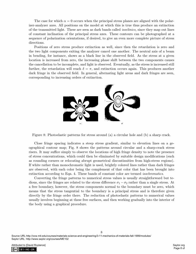
Figure 8: Photoelastic patterns for stress around (a) a circular hole and (b) a sharp crack.
Close fringe spacing indicates a steep stress gradient, similar to elevation lines on a ge-ographical contour map; Fig. 8 shows the patterns around circular and a sharp-crack stressrisers. It may suffice simply to observe the locations of high fringe density to note the presenceof stress concentrations, which could then be eliminated by suitable design modifications (suchas rounding corners or relocating abrupt geometrical discontinuities from high-stress regions).If white rather than monochromatic light is used, brightly colored lines rather than dark fringesare observed, with each color being the complement of that color that has been brought intoextinction according to Eqn. 4. These bands of constant color are termed isochromatics.Converting the fringe patterns to numerical stress values is usually straightforward but te-
dious, since the fringes are related to the stress difference σ1−σ2 rather than a single stress. Ata free boundary, however, the stress components normal to the boundary must be zero, whichmeans that the stress tangential to the boundary is a principal stress and is therefore givendirectly by the fringe order there. The reduction of photoelastic patterns to numerical valuesusually involves beginning at these free surfaces, and then working gradually into the interior ofthe body using a graphical procedure.
8Source URL:http://ocw.mit.edu/courses/materials-science-and-engineering/3-11-mechanics-of-materials-fall-1999/modules/ Saylor URL: http://www.saylor.org/courses/ME102 Attributed to [David Roylance]
Saylor.org Page 8 of

Moire
The term “moire” is spelled with a small “m” and derives not from someone’s name but fromthe name of a silk fabric that shows patterns of light and dark bands. Bands of this sort are alsodeveloped by the superposition of two almost-identical gratings, such as might be seen whenlooking through two window screens slightly rotated from one another. Figure 9 demonstratesthat fringes are developed if the two grids have different spacing as well as different orientations.The fringes change dramatically for even small motions or strains in the gratings, and this visualamplification of motion can be used in detecting and quantifying strain in the specimen.
Figure 9: Moire fringes developed by difference in line pitch (a) and line orientation (b). (Prof.Fu-Pen Chiang, SUNY-Stony Brook.)
As a simple illustration of moire strain analysis, assume a grating of vertical lines of spacing p(the “specimen” grating) is bonded to the specimen and that this is observed by looking throughanother “reference” grating of the same period but not bonded to the specimen. Now let thespecimen undergo a strain, so that the specimen grating is stretched to a period of p′. A darkfringe will appear when the lines from the two gratings superimpose, and this will occur whenN(p′ − p) = p, since after N lines on the specimen grid the incremental gap (p′ − p) will haveaccumulated to one reference pitch distance p. The distance S between the fringes is then
S = Np′ =pp′
p′ − p(7)
The normal strain εx in the horizontal direction is now given directly from the fringe spacing as
εx =p′ − p
p=p
S(8)
Fringes will also develop if the specimen grid undergoes a rotation relative to the referencegrid: if the rotation is small, then
p
S= tan θ ≈ θ
S =p
θ
This angle is also the shear strain γxy, so
γxy = θ =p
θ(9)
More generally, consider the interference fringes that develop between a vertical reference gridand an arbitrarily displaced specimen grid (originally vertical). The zeroth-order (N = 0) fringeis that corresponding to positions having zero horizontal displacement, the first-order (N = 1)
9Source URL:http://ocw.mit.edu/courses/materials-science-and-engineering/3-11-mechanics-of-materials-fall-1999/modules/ Saylor URL: http://www.saylor.org/courses/ME102 Attributed to [David Roylance]
Saylor.org Page 9 of

fringe corresponds to horizontal motions of exactly one pitch distance, etc. The horizontaldisplacement is given directly by the fringe order as u = Np, from which the strain is given by
εx =∂u
∂x= p∂N
∂x(10)
so the strain is given as the slope of the fringe.Similarly, a moire pattern developed between two originally horizontal grids, characterized
by fringes N ′ = 0, 1, 2, · · · gives the vertical strains:
εy =∂v
∂y=∂(N ′p)
∂y= p∂N ′
∂y(11)
The shearing strains are found from the slopes of both the u-field and v-field fringes:
γxy = p
(∂N
∂y+∂N ′
∂x
)(12)
Figure 10 shows the fringes corresponding to vertical displacements around a circular holein a plate subjected to loading in the y-direction. The vertical strain εy is proportional to they-distance between these fringes, each of which is a contour of constant vertical displacement.This strain is largest along the x-axis at the periphery of the hole, and smallest along the y-axisat the periphery of the hole.
Figure 10: Moire patterns of the vertical displacements of a bar with a hole under pure tension.(Prof. Fu-Pen Chiang, SUNY-Stony Brook.)
Problems
1. A 0/45/90three-arm strain gage rosette bonded to a steel specimen gives readings ε0 =175µ, ε45 = 150 µ, and ε90 = −120 µ. Determine the principal stresses and the orientationof the principal planes at the gage location.
2. Repeat the previous problem, but with gage readings ε0 = 150 µ, ε45 = 200 µ, andε90 = 125 µ.
10Source URL:http://ocw.mit.edu/courses/materials-science-and-engineering/3-11-mechanics-of-materials-fall-1999/modules/ Saylor URL: http://www.saylor.org/courses/ME102 Attributed to [David Roylance]
Saylor.org Page 10 of
Copyright © 2022 FDOKUMEN