materials

Article

Experimental and Numerical Study of the Elastic SCF ofTubular Joints

Mostafa Atteya 1,* , Ove Mikkelsen 1, John Wintle 2 and Gerhard Ersdal 1

�����������������

Citation: Atteya, M.; Mikkelsen, O.;

Wintle, J.; Ersdal, G. Experimental

and Numerical Study of the Elastic

SCF of Tubular Joints. Materials 2021,

14, 4220. https://doi.org/10.3390/

ma14154220

Academic Editors: Jarosław Jedrysiak,

Izabela Lubowiecka and

Ewa Magnucka-Blandzi

Received: 30 June 2021

Accepted: 26 July 2021

Published: 28 July 2021

Publisher’s Note: MDPI stays neutral

with regard to jurisdictional claims in

published maps and institutional affil-

iations.

Copyright: © 2021 by the authors.

Licensee MDPI, Basel, Switzerland.

This article is an open access article

distributed under the terms and

conditions of the Creative Commons

Attribution (CC BY) license (https://

creativecommons.org/licenses/by/

4.0/).

1 Department of Mechanical and Structural Engineering and Materials Science, Faculty ofScience and Technology, University of Stavanger, 4021 Stavanger, Norway; ove.mikkelsen@uis.no (O.M.);gerhard.ersdal@uis.no (G.E.)

2 Department of Mechanical Engineering, Faculty of Engineering, University of Strathclyde,Glasgow G1 1XQ, UK; john.b.wintle@gmail.com

* Correspondence: mostafa.a.atteya@uis.no

Abstract: This paper provides data on stress concentration factors (SCFs) from experimental measure-ments on cruciform tubular joints of a chord and brace intersection under axial loading. High-fidelityfinite element models were generated and validated against these measurements. Further, the statis-tical variation and the uncertainty in both experiments and finite element analysis (FEA) are studied,including the effect of finite element modelling of the weld profile, mesh size, element type and themethod for deriving the SCF. A method is proposed for modelling such uncertainties in order todetermine a reasonable SCF. Traditionally, SCF are determined by parametric formulae found in codesand standards and the paper also provides these for comparison. Results from the FEA generallyshow that the SCF increases with a finer mesh, 2nd order brick elements, linear extrapolation anda larger weld profile. Comparison between experimental SCFs indicates that a very fine mesh andthe use of 2nd order elements is required to provide SCF on the safe side. It is further found thatthe parametric SCF equations in codes are reasonably on the safe side and a detailed finite elementanalysis could be beneficial if small gains in fatigue life need to be justified.

Keywords: fatigue; offshore structures; experimental testing; tubular joints; hot spot stress (HSS);stress concentration factors (SCF); finite element analysis (FEA)

1. Introduction

Fixed steel offshore structures (jackets) are framed structures of tubular memberswelded together. These are the most common type of offshore substructure for oil andgas exploration and to an increasing degree also being used for offshore wind turbines.The structures are exposed to cyclic wave and wind loads in corrosive environments andfatigue is one of the main design criteria. The fatigue life assessment of welded joints istypically based on S–N curves in combination with a damage rule. The assumption oflinear cumulative damage using the Palmgren–Miner rule is widely applied [1].

Design S–N curves for various classes of welded joints have been established primarilybased on test specimens in the laboratory [2]. Due to the geometry of welded tubular joints,high-stress gradients exist in the transition zone between the weld line and the basematerial, and in linear stress analysis, the geometric discontinuity of the weld toe defines astress singularity.

In general, stresses in tubular joints arises from three main causes, excluding theresidual or misfit stresses as shown in Figure 1; these are the nominal stresses: stressesin the members under applied external loads without considering the detail of the jointintersection, i.e., the framing action of the jacket structure under applied external loads.Hot spot stress (deformation stresses): stresses close to the weld toe arising from thedeformation of the tubular wall to maintain continuity at the intersection with the weld

Materials 2021, 14, 4220. https://doi.org/10.3390/ma14154220 https://www.mdpi.com/journal/materials

Materials 2021, 14, 4220 2 of 20

profile under the applied external loads. Finally, notch stress: stresses introduced due tothe geometrical discontinuity at the weld toe/root.

Figure 1. Definition of tubular joint stresses.

In stress analysis, hot-spot stress is the highest value of stress that can be inferred asnear the weld as possible, generally at the weld toe. It can be estimated by modifying thenominal cyclic stress arising from the loads in the joint by a stress concentration factor(SCF). The SCF is intended to incorporate the stress of the local joint geometry and thediscontinuity but omits the influence of the weld toe itself.

In practice, the tubular joint SCF is usually calculated from parametric equationsgiven in standards such as ISO 19902 [1], API RP2A [3] and DNVGL-RP-C203 [4] or fromcase-by-case finite element analysis. The standard and code-based SCFs are expected toprovide upper-bound values for use in design and life extension assessments.

Various parametric formulas, expressed with non-dimensional joint parameters fordifferent types of loading and boundary conditions, have been developed both experimen-tally and numerically. Beale and Toprac [5], used small scale T and KT joints under tensileloading. Reber [6] and Visser [7] attempted to estimate the hot-spot stress of T, Y and Kjoints under compression loading using finite-element programs. Marshall [8] adopted theKellogg [9] formula to express SCF for brace and chord of K joints using classical solutionmethods. Kuang et al. [10] used finite element analysis to develop semi-empirical formulaeto cover the SCF on brace and chord side for 138 T, Y, K and KT joints. Gibstein [11] carriedout parametric analysis for seventeen T joints using FE analysis to investigate rigidlyfixed chord ends. Wordsworth and Smedley [12] presented one of the first comprehensiveparametric formulae for SCFs of T,Y, KT and DT joints. The parametric study was obtainedfrom acrylic model testing. Later Efthymiou [13] provided generalised influence functionsdeveloped for use in fatigue analysis. The SCFs are derived by establishing influencefunctions describing the ‘hot spot’ stress at a particular location of a specific member. Ithas been developed by performing finite element analyses using the in-house PMBSHELLprogram. The program uses thick shell elements for modelling the members and 3-D brickelements for the weld. The influence functions by Efthymiou are implemented in codesand standards and are the most widely used currently.

Smedley and Fisher [14] concluded that since Efthymiou SCFs are design formulaegiving a mean fit to his FE database, it tends to underpredict in 20–40% of the casescompared to Lloyd’s Register experimental database consisting of steel and acrylic models.Hence, the first impression of this indication could be that Efthymiou formulae provide SCFvalues on the unsafe side of the database. However, ISO 19902 [1] indicates that Efthymiou’parametric formulae have a bias of 19% to the safe side compared to the experimental values,with a coefficient of variation (CoV) of 19% (20% according to DNVGL-RP-C210 [15]). The

Materials 2021, 14, 4220 3 of 20

formulae have been accepted as providing a reliable design basis for structures withtubular joints.

The parametric equations have been typically developed from extrapolated exper-imental strain gauge measurements or generic finite element analysis of representativetest joints. Although case-by-case finite element analysis methods use linear extrapolationfrom the same points typically used to place strain gauges in experiments, this approachoverlooks the weld profile tolerances captured in tests. As a result, the analyst cannotnormally incorporate the as-built weld profile into a model accurately. Thus, in some cases,the numerical finite element values could underestimate the SCF compared with thosederived from parametric equations and experiments.

This paper presents a review and comparison between case-by-case finite elementanalysis and experimental and parametric estimates of SCF for cruciform tubular joints(also called double T or X joints based on the specific structural behaviour) with geometricparameters of β = 0.5, τ = 1 and θ = 90◦ under axial loading.

Experimentally determined SCFs were derived from multiple strain gauge measure-ments made on four test specimens loaded in a fatigue rig. Stress concentration factorsare obtained at four points along the joint periphery from the chord saddle to the chordcrown. These were compared with results from finite element models with idealised weldprofiles and models with weld profiles matched to the test specimens and with the valuescalculated from the standard parametric equations.

2. Design Stress Concentration Factor (SCF)

This section presents a comparison between the available formulae to estimate theSCFs of a DT joint then compare it to the existing database. Finally, it provides an estimatefor the SCFs distribution along the brace-to-chord intersection from design SCFs andprevious experimental work.

2.1. Existing Parametric Formulae

Two parametric equations do exist to estimate the chord saddle SCFs of DT joints,namely, Wordsworth/Smedley (1) and Efthymiou (2).

SCFchord (saddle) = 1.7βγτ(

2.42− 2.28β2.2)

sinβ2(15−14.4β) θ (1)

SCFchord (saddle) = 3.87γτβ(

1.1− β1.8)(sin θ)1.7 (2)

where β = d/D, γ = D/2T and τ = t/T;

t brace wall thickness;T chord wall thickness;d brace outside diameter;D chord outside diameter;θ is the angle between the brace and the chord.

A comparison of the variation in the chord saddle SCF for β and τ between thetwo sets of formulae are given in Figures 2 and 3. The expression of chord saddle fromEfthymiou and Wordsworth/Smedley showed that both expressions have slight to nodifference. Under constant τ, Wordsworth and Smedley’s expression show higher SCF bysome 2% than Efthymiou for midrange β values while Efthymiou shows higher valuesthan Wordsworth and Smedley at β higher than 0.9. Under constant β, Wordsworth showshigher values than Efthymiou by 3% for any τ value.

Materials 2021, 14, 4220 4 of 20

Figure 2. Axially loaded DT joints: chord SCF variation with 𝛽 for a set of joint

parameters (𝜃, 𝛾 and 𝜏).

Figure 3. Axially loaded DT joints: chord SCF variation with 𝜏 for a set of joint

parameters (𝜃, 𝛾 and 𝛽).

Figure 4. Existing database for DT joints under axial loading.

2

6

10

14

18

22

26

0.2 0.4 0.6 0.8 1.0

SCF

Ch

ord

Sad

dle

β

EfthymiouWordsworth/SmedleySpecimens

𝜏 = 1.0,𝛾 = 13.4,𝜃 = 90°

2

6

10

14

18

22

26

0.2 0.4 0.6 0.8 1.0

SCF

Ch

ord

Sad

dle

𝜏

Wordsworth/SmedleyEfthymiouSpecimens

𝛽 = 0.5,𝛾 = 13.4,𝜃 = 90°

0

5

10

15

20

25

0 5 10 15 20 25

SCF

-Ef

thym

iou

,W

ord

swo

rth

an

d S

med

ley

SCF - Previous Experimental work

Efthymiou

Wordsworth and Smedley

20% bias

lines

Figure 2. Axially loaded DT joints: chord SCF variation with β for a set of joint parameters (θ, γ and τ ).

Figure 2. Axially loaded DT joints: chord SCF variation with 𝛽 for a set of joint

parameters (𝜃, 𝛾 and 𝜏).

Figure 3. Axially loaded DT joints: chord SCF variation with 𝜏 for a set of joint

parameters (𝜃, 𝛾 and 𝛽).

Figure 4. Existing database for DT joints under axial loading.

2

6

10

14

18

22

26

0.2 0.4 0.6 0.8 1.0

SCF

Ch

ord

Sad

dle

β

EfthymiouWordsworth/SmedleySpecimens

𝜏 = 1.0,𝛾 = 13.4,𝜃 = 90°

2

6

10

14

18

22

26

0.2 0.4 0.6 0.8 1.0

SCF

Ch

ord

Sad

dle

𝜏

Wordsworth/SmedleyEfthymiouSpecimens

𝛽 = 0.5,𝛾 = 13.4,𝜃 = 90°

0

5

10

15

20

25

0 5 10 15 20 25

SCF

-Ef

thym

iou

,W

ord

swo

rth

an

d S

med

ley

SCF - Previous Experimental work

Efthymiou

Wordsworth and Smedley

20% bias

lines

Figure 3. Axially loaded DT joints: chord SCF variation with τ for a set of joint parameters (θ, γ and β ).

2.2. Comparison with Previous Experimental Results

There is a limited amount of published data on the SCFs of DT tubular joints, which canbe compared to Efthymiou and Wordsworth and Smedley parametric equations. However,some published data collected from the literature [16–19] are included in this comparison.

A comparison of the published data is shown in Figure 4 (within the validity range asper the codes and standards). In this comparison it was found that Efthymiou data shows abias of 20% on the safe side while the Wordsworth and Smedley SCF estimate shows a biasof 22% on the safe side, reasonably in line with the findings of ISO 19902 [1] mentionedearlier. Hence it can be concluded that Efthymiou provides a closer estimate to the realSCFs than Wordsworth and Smedley except for cases with β higher than 0.9.

Figure 2. Axially loaded DT joints: chord SCF variation with 𝛽 for a set of joint

parameters (𝜃, 𝛾 and 𝜏).

Figure 3. Axially loaded DT joints: chord SCF variation with 𝜏 for a set of joint

parameters (𝜃, 𝛾 and 𝛽).

Figure 4. Existing database for DT joints under axial loading.

2

6

10

14

18

22

26

0.2 0.4 0.6 0.8 1.0

SCF

Ch

ord

Sad

dle

β

EfthymiouWordsworth/SmedleySpecimens

𝜏 = 1.0,𝛾 = 13.4,𝜃 = 90°

2

6

10

14

18

22

26

0.2 0.4 0.6 0.8 1.0

SCF

Ch

ord

Sad

dle

𝜏

Wordsworth/SmedleyEfthymiouSpecimens

𝛽 = 0.5,𝛾 = 13.4,𝜃 = 90°

0

5

10

15

20

25

0 5 10 15 20 25

SCF

-Ef

thym

iou

,W

ord

swo

rth

an

d S

med

ley

SCF - Previous Experimental work

Efthymiou

Wordsworth and Smedley

20% bias

lines

Figure 4. Existing database for DT joints under axial loading.

Materials 2021, 14, 4220 5 of 20

2.3. SCFs Distribution at the Brace-to-Chord Intersection

Efthymiou provides SCFs for the saddle and crown point of a tubular joint. Forjoints under pure axial loading, linear interpolation is then recommended to estimatestresses at points between the saddle and crown [20]. Table 1 shows the estimated SCFsfrom the chord saddle to crown based on design Efthymiou SCFs and data from previousexperimental work.

Table 1. SCFs from the chord saddle to crown based on design Efthymiou SCFs and previousexperimental work.

Location Efthymiou Average of PreviousExperimental Work [16–19]

0◦ Saddle 22.35 18.8222.5◦ 17.55 14.7945◦ 12.76 10.76

90◦ Crown 3.16 2.69

3. Experimental Stress Concentration Factor (SCF)

This section presents the stress distribution at the brace/chord intersection and SCFsfrom present experimental work. It is a part of experimental testing to study crack arrestingtechniques in tubular joints. The testing program for the specimens is to undergo cyclicloading until precracking (developing a through-thickness crack), then crack arresting bymeans of hole drilling followed by cyclic reloading until failure. Strain gauges are mountedon the specimen to map the stresses at the joint intersection and estimate the SCF during allthe fatigue loading stages. The SCFs of interest in this paper are estimated from the initialload before commencing the precracking stage.

3.1. Specimen Design

Four DT joints fabricated with dimensions of 219.1 mm outer chord diameter (D) with8.2 mm chord wall thickness (T) and 114.3 mm brace outer diameter (d) with 8.5 mm bracewall thickness (t) with geometric factors of β = d/D = 0.5, τ = t/T = 1 and chord tobrace angle θ of 90◦ as shown in Figure 5.

Figure 5. DT Joint geometry (all units are in mm).

All the steelwork fabrication, inspection and testing were done in accordance withDNV-OS-C401 [21]. The welded specimen underwent a detailed dimensional and visualinspection to ensure that all the dimensions and welded details are within specifications.

Materials 2021, 14, 4220 6 of 20

3.2. Methodology for Determining Stress Concentration Factors

The distribution of stresses at the brace-to-chord intersection is measured by straingauges perpendicular (HBM, Darmstadt, Germany) to the weld toe for all the specimensunder tensile axial loading. Test Specimens setup are presented in Figure 6.

Figure 6. Test specimens setup.

The stress concentration factor (SCF) or strain concentration factor (SNCF) are definedas the ratio of the hot spot stress or strain to the calculated nominal brace stress or strain.Hot spot stresses can be determined by extrapolating stresses from the given points toestimate the stress at the weld toe. This approach distinguishes the hot-spot (deformation)stress from the notch stress and uses the given points for measurements outside the notchregion. Three methods of extrapolation were adopted in a study by the department ofenergy [22] to determine the hot spot stress to calculate the SCF subsequently:

(1) Method A: Linear extrapolation of maximum principal stresses.(2) Method B: Curvilinear extrapolation of maximum principal stresses.(3) Method C: Curvilinear extrapolation of strains perpendicular to the weld toe.

The study concluded that the curvilinear extrapolation of maximum principal stresseswas 10% higher than the linear method. In later studies [22–24], it was determined to usemethod A, the linear extrapolation, as the method of ‘hot spot’ SCF determination to beused with the S–N curves for tubular joints. The method was adopted in the current codesand standards.

3.3. Loading Procedure

Nominal stresses were estimated by measuring the load applied on the brace from therig built-in load cell and the brace’s cross-sectional dimensions, which were measured toan accuracy of 10−2 mm.

Fifty percent (50%) of the yielding strain was applied for 100 sinusoidal load cycles toa strain of approximately 700 microstrains at the chord saddle to ‘shake down’ the straingauges. After ‘shake down’, the specimens were loaded for 200 cycles for a hot spot stressrange of approximately 280 MPa with a load frequency of 3 Hz. Based on 200 Hz readingsthe data was interpolated to determine average response range for the estimation of SNCFs.

Materials 2021, 14, 4220 7 of 20

This technique was applied to stabilise the response in the joint and to minimize eventualdata acquisition errors.

3.4. Strain Gauge Locations, Data Logging and Processing

The strain gauges were glued to the chord and brace members to determine the stressdistribution on the chord side from the saddle to the crown and nominal stresses in bracemembers. The chord saddle strain gauges layout is shown in Figure 7. The method ofextrapolation used for each specimen tested was the linear extrapolation method. Straingauge locations were placed based on the recommendation from the UKOSRP [25–27]project. The strain gauge locations to be located outside the notch region, with the firstpoint defined as the greatest of 0.2

√rt and 4 mm. The second point was located at the

brace-to-chord intersection according to the location:

(1) Chord saddle = πR/36;(2) Chord crown = 0.4 4

√rtRT;

(3) Brace side = 0.65√

rt.

where r is the brace outer radius and R is the chord outer radius.

Figure 7. Chord saddle strain gauge layout.

Based on the recommendations above, the first row of strain gauges on the chord sidewas intended to be glued with its centre located at 4.42 mm from the weld toe, while thesecond row of gauges was intended to be glued with a varying distance of 9.56 mm fromthe weld toe at the chord saddle and 10.29 mm from the weld toe and chord crown.

Due to the space limitation on the chord saddle, only linear strain gauges perpendicu-lar to the weld toe were glued and lateral strain gauges were omitted. The strains measuredas-is from this layout was not sufficient to calculate the maximum principal stresses. Astudy by Lloyd’s Register tested three ways of calculating the SCF from the strain gaugeresults [28]:

(a) Extrapolation of maximum principal stresses.(b) Extrapolation of the strains perpendicular to the weld toe.(c) Conversion of the SNCF in method (b) to biaxial stress.

The study [28] found that for 90◦ joints, the maximum principal stress estimatedwith method (a) was approximately 15% larger than the directional stresses based onmethod (b).

This study applies experimental strain measurements combined with FE analysis toestimate the principal stresses. The measured strains perpendicular to the weld toe arepresented in Table 2 and used to validate the FE analysis. The analysis was performed

Materials 2021, 14, 4220 8 of 20

using linear and quadratic elements with the linear extrapolation method to estimate theSCFs based on directional and maximum principal stresses. The range of results from FEanalysis are shown in Table 2.

Table 2. Experimental measured strain concentration factors (SNCF), FE validation and SCF correc-tion factors from directional stresses perpendicular to the weld toe to principal stresses.

Location 0◦—Saddle 22.5◦ 45◦ 90◦—Crown

SNCF—directional (mean) 17.28 14.76 8.77 2.15SNCF—directional (Std. dev.) 1.49 1.50 1.01 0.26

FE SCF—directional 16.67–18.34 13.37–15.02 7.87–9.03 2.28–2.28FE SCF—maximum principal 19.12–21.03 15.35–17.22 9.06–10.38 2.68–2.68

Correction factor 14.7% 14.8% 15.2% 17.6%

The FE analysis showed that the principal stresses at the saddle were 14.7% higherthan the perpendicular stresses and increased slightly towards the crown, reaching 17.6%.The results are in line with the study by Lloyd’s Register [28]. In the present work, thecorrection factors as presented in Table 2 were used to estimate the principal stresses atdifferent locations from the experimentally measured strains perpendicular to the weld toe.Details of the FE analysis are presented in Section 4.

3.5. Experimental Work Results

The experimental work presented herein followed method b, as described in Section 3.4,for the SCF extrapolation from strain gauges. Hence, the SCFs from the experimental workwere updated by correction factors as per Table 2 to be compatible with the parametric codeequations (Efthymiou formulae [13]) and the SCFs extracted from FE models.

The distribution of stresses along the circumference of the brace to chord intersectionas measured by linear extrapolation of principal stresses for all the specimen tested arepresented in Figure 8 and Table 3. The distribution was plotted along the intersection withreference to an angular position from the saddle at 0◦ to the crown at 90◦.

Figure 8. Experimental hot spot SCF along the weld toe from the saddle (0°) to

crown (90°).

Figure 9. SCF values from experimental work plotted in a normal distribution

paper, indicating a mean value of the SCF of 19.87 and a standard deviation of 2.

0

5

10

15

20

25

0 22.5 45 67.5 90

Ho

t sp

ot

SCF

Angle from saddle (0°) to crown (90°)

Specimen DT 1

Specimen DT 2

Specimen DT 3

Specimen DT 4

Upper bound

Lower bound

y = 0.4998x - 9.9322R² = 0.9832

-2

-1.5

-1

-0.5

0

0.5

1

1.5

2

17 18 19 20 21 22 23 24

Sam

ple

qu

anti

les

SCF

Figure 8. Experimental hot spot SCF along the weld toe from the saddle (0◦) to crown (90◦).

Materials 2021, 14, 4220 9 of 20

Table 3. SCFs from experimental work (present data).

Specimen Location Saddle * 22.5◦ 45◦ Crown

DT 1Number of points 4 8 8 -

SCF (mean) 18.43 15.74 9.27 -Std. dev. 0.55 1.57 0.69 -

DT 2Number of points 4 - - 4

SCF (mean) 20.36 - - 2.53Std. dev. 1.06 - - 0.31

DT 3Number of points 3 7 7 -

SCF (mean) 19.79 17.78 11.27 -Standard deviation 2.54 1.17 0.94 -

DT 4Number of points 4 8 7 -

SCF (mean) 20.88 17.50 9.87 -Std. dev. 1.93 1.89 0.87 -

Entire sample(DT 1, DT 2,

DT 3 and DT 4)

Number of points 15 23 22 4SCF (mean) 19.87 16.98 10.10 2.53

Std. dev. 1.72 1.73 1.17 0.31Coeff. of variation 8.7% 10.2% 11.6% 12.2%

* Angle measured from the chord saddle centre.

The distribution of the SCF’s at the saddle point from the experimental work fitreasonably well the normal distribution, as shown in Figure 9. By bootstrapping the data, itis indicated that the 90% confidence interval for the mean value of the SCF was [19.3, 20.6]and for the standard deviation [1.2, 2.1], providing a CoV in the range of 5–10%.

Figure 8. Experimental hot spot SCF along the weld toe from the saddle (0°) to

crown (90°).

Figure 9. SCF values from experimental work plotted in a normal distribution

paper, indicating a mean value of the SCF of 19.87 and a standard deviation of 2.

0

5

10

15

20

25

0 22.5 45 67.5 90

Ho

t sp

ot

SCF

Angle from saddle (0°) to crown (90°)

Specimen DT 1

Specimen DT 2

Specimen DT 3

Specimen DT 4

Upper bound

Lower bound

y = 0.4998x - 9.9322R² = 0.9832

-2

-1.5

-1

-0.5

0

0.5

1

1.5

2

17 18 19 20 21 22 23 24

Sam

ple

qu

anti

les

SCF

Figure 9. SCF values from experimental work plotted in a normal distribution paper, indicating amean value of the SCF of 19.87 and a standard deviation of 2.

3.6. Review of the Accuracy of Experimental SCFs

The precision in the strain gauge’s locations was studied at eight locations of thechord side saddle from two randomly selected specimens of the total of four. The variationbetween actual and average strain gauge location is a useful indicator of the overallaccuracy of the SCF for the specimen. The actual strain gauge’s locations to the weld toewere measured to an accuracy of ±0.1 mm, then the measured points and their strainreadings were used to extrapolate for the SCFs linearly. The results show that the locationof the strain gauges at point “a” were scattered without evidence of any systematic error.However, for the strain gauges at point “b” there is a scatter around a mean shift of 1.1 mmfrom the intended “b” location. The shift in mean value can be explained by the lengthof the strain gauge carriers. The carrier’s length was 5 mm while the difference betweenpoint “a” and “b” was only 5.1 mm, which made it challenging to manually position thestrain gauges spot on. Figure 10 shows the distribution of strain gauges along the weldtoe’s intended “a” and “b” locations and the extrapolation lines to the SCF value for each

Materials 2021, 14, 4220 10 of 20

pair of points. After strain gauges installation, the average distance between “a” and “b”was approximately 6.3 mm.

Figure 10. Experimentally measured SCFs sensitivity.

Figure 14. Direct and linear extrapolation of SCF from first-order 8-node brick

elements.

8

10

12

14

16

18

20

22

0.0 2.0 4.0 6.0 8.0 10.0 12.0 14.0

Ho

t sp

ot

stre

ss /

No

min

al s

tres

s

Distance from Brace weld toe (mm)

Measured a

Measured b

𝑎=0.2

𝑟𝑡

𝑏=𝜋𝑅/36

𝑊𝑒𝑙𝑑𝑡𝑜𝑒

0

5

10

15

20

25

30

35

0 2 4 6 8 10 12

Ho

t sp

ot

stre

ss /

no

min

al s

tres

s

Distance from brace weld toe (mm)

Unaveraged Principle Stresses

Linear Extrapolation

Direct Extraction

𝑎=0.2

𝑟𝑡

0.1ξ𝑟𝑡

𝑏=𝜋𝑅/36

Figure 10. Experimentally measured SCFs sensitivity.

The average SCF measured at the chord saddle from these eight points was 18.71 witha standard deviation of 1.21, providing a CoV of 6.5%, while the uncorrected average forthe same two specimens provides a mean SCF of 19.4 with a CoV of 8.4%. The differencebetween the mean value between these two samples can be assumed to be due to inaccuracyin the strain gauge locations, while the variation between the results from the eight pointswas a combination of other inherent uncertainty (geometry, material, measurement, etc.).

This implies that the shift in strain gauge location introduces a bias of 3.7% to the safeside, which can also easily be seen to be reasonable by a geometric evaluation. For theentire sample, the average SCF was found to be 19.87 with a standard deviation of 1.72and CoV of 8.7%. To adjust for the strain gauge location, assuming the same trend for thetwo remaining specimens as for the two tested, the mean value of the SCF should be set to19.87/1.037 = 19.16 and a CoV of 8.4%.

In summary, it can be concluded from the obtained statistical coefficients that theaverage test values were in good agreement with the actual values and the data can betreated as valid. The test data was further verified by correlation with the finite elementsand available parametric formulae.

4. Finite Element Analysis Based SCFs

This section presents finite element analysis to estimate SCFs of DT joints consid-ering the effect of the weld profile variation and the methodology of modelling on theSCFs results.

4.1. Modelling and Analysis Approach

The DT joint consists of a 219.1 mm × 8.2 mm member with an adjoining114.3 mm × 8.5 mm member. The geometry is considered to reflect a single-sided weldmade from the outside. During the fabrication, the joint braces were cut so that the braceinner circumference matched the chord profile. The braces were then joined to the chord withsingle-sided welds.

4.2. Weld Profile

The weld details were as per the weld preparation instructions shown in Figure 11.The weld at the saddle was assumed to be of weld location 2, as shown in the weld detailsdrawing and the weld at the crown was assumed weld location 1.

Materials 2021, 14, 4220 11 of 20

Figure 11. Weld profile specifications as issued to the fabricator for these tests in line with appropriate standards, see Section 4.4.

Specimen DT1 was cut into segments post-testing each 20◦ from the saddle to thecrown to measure the weld profile’s cross-section at the brace-to-chord intersection accu-rately. The shape of the weld profile modelled was based on the measured cut segmentsshown in Figure 12. At the saddle, the brace was cut back to normal to the axis of the bracecylinder. At the crown, the parent material was assumed to be cut back to approximately45◦ and then filled so that the intersection between the weld and the brace was at a rightangle. The weld profile was a smooth transition based on an elliptical profile between thecut segments.

Figure 12. Actual weld profile cut from one of the specimens.

The weld toe and root radii were omitted for simplicity. They were unlikely to affectthe resulting hot spot stress as this was extrapolated from points sufficiently away fromthe sharp corners.

4.3. Model Description

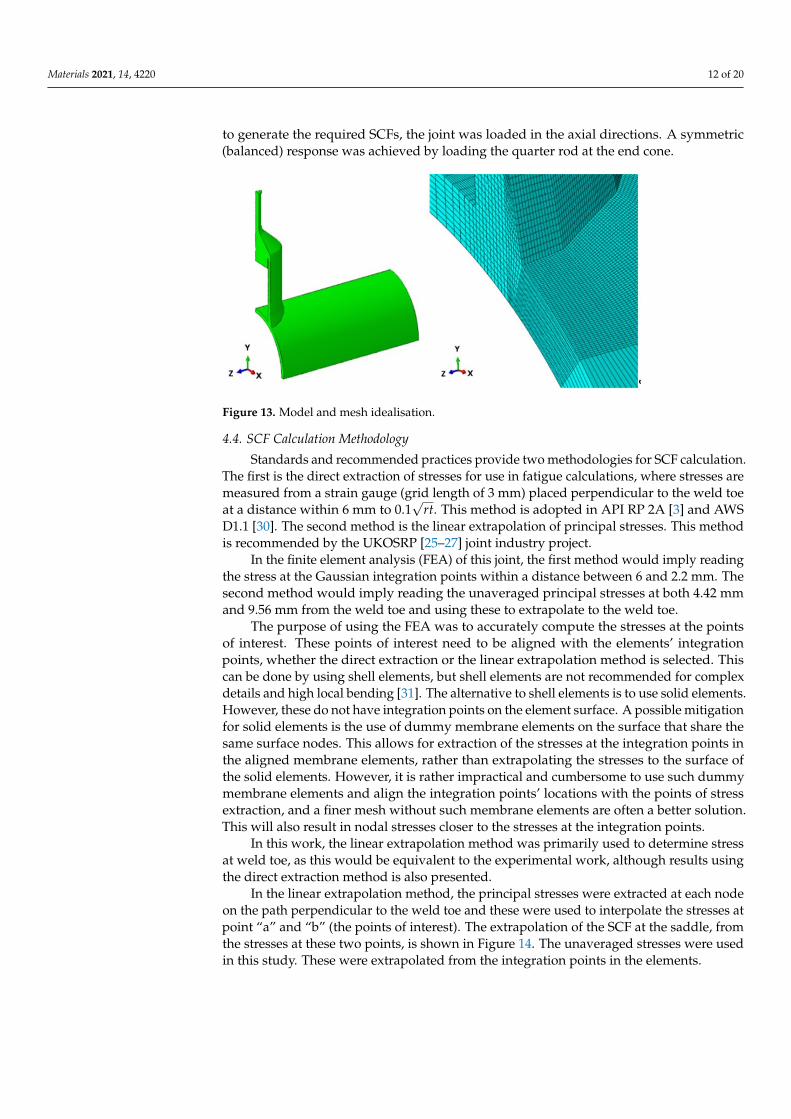
The 3D model was developed using Dassault Systems Abaqus [29]. The DT joint wasmodelled using first order C3D8R and second order C3D20R hexahedron elements for thejoint stubs with a characteristic element size of 1 mm at the chord to brace intersection.This mesh size provided nine elements through-thickness. A coarser representation of theouter extents of the tubular members was created using the same elements to a distance ofapproximately 40 mm from the weld (see Figure 13). The end cone was modelled at thebrace ends to capture as accurately as possible to the actual joint behaviour. The joint wassymmetric about the three principal planes. Only one-eighth of the joint was modelled.The saddles occurred at 0◦ and the crowns at 90◦. All material (parent and weld filler)was linear elastic with a Young’s modulus of 207 GPa and Poisson’s ratio of 0.3. In order

Materials 2021, 14, 4220 12 of 20

to generate the required SCFs, the joint was loaded in the axial directions. A symmetric(balanced) response was achieved by loading the quarter rod at the end cone.

Figure 13. Model and mesh idealisation.

4.4. SCF Calculation Methodology

Standards and recommended practices provide two methodologies for SCF calculation.The first is the direct extraction of stresses for use in fatigue calculations, where stresses aremeasured from a strain gauge (grid length of 3 mm) placed perpendicular to the weld toeat a distance within 6 mm to 0.1

√rt. This method is adopted in API RP 2A [3] and AWS

D1.1 [30]. The second method is the linear extrapolation of principal stresses. This methodis recommended by the UKOSRP [25–27] joint industry project.

In the finite element analysis (FEA) of this joint, the first method would imply readingthe stress at the Gaussian integration points within a distance between 6 and 2.2 mm. Thesecond method would imply reading the unaveraged principal stresses at both 4.42 mmand 9.56 mm from the weld toe and using these to extrapolate to the weld toe.

The purpose of using the FEA was to accurately compute the stresses at the pointsof interest. These points of interest need to be aligned with the elements’ integrationpoints, whether the direct extraction or the linear extrapolation method is selected. Thiscan be done by using shell elements, but shell elements are not recommended for complexdetails and high local bending [31]. The alternative to shell elements is to use solid elements.However, these do not have integration points on the element surface. A possible mitigationfor solid elements is the use of dummy membrane elements on the surface that share thesame surface nodes. This allows for extraction of the stresses at the integration points inthe aligned membrane elements, rather than extrapolating the stresses to the surface ofthe solid elements. However, it is rather impractical and cumbersome to use such dummymembrane elements and align the integration points’ locations with the points of stressextraction, and a finer mesh without such membrane elements are often a better solution.This will also result in nodal stresses closer to the stresses at the integration points.

In this work, the linear extrapolation method was primarily used to determine stressat weld toe, as this would be equivalent to the experimental work, although results usingthe direct extraction method is also presented.

In the linear extrapolation method, the principal stresses were extracted at each nodeon the path perpendicular to the weld toe and these were used to interpolate the stresses atpoint “a” and “b” (the points of interest). The extrapolation of the SCF at the saddle, fromthe stresses at these two points, is shown in Figure 14. The unaveraged stresses were usedin this study. These were extrapolated from the integration points in the elements.

Materials 2021, 14, 4220 13 of 20

Figure 10. Experimentally measured SCFs sensitivity.

Figure 14. Direct and linear extrapolation of SCF from first-order 8-node brick

elements.

8

10

12

14

16

18

20

22

0.0 2.0 4.0 6.0 8.0 10.0 12.0 14.0

Ho

t sp

ot

stre

ss /

No

min

al s

tres

s

Distance from Brace weld toe (mm)

Measured a

Measured b

𝑎=0.2

𝑟𝑡

𝑏=𝜋𝑅/36

𝑊𝑒𝑙𝑑𝑡𝑜𝑒

0

5

10

15

20

25

30

35

0 2 4 6 8 10 12

Ho

t sp

ot

stre

ss /

no

min

al s

tres

s

Distance from brace weld toe (mm)

Unaveraged Principle Stresses

Linear Extrapolation

Direct Extraction

𝑎=0.2

𝑟𝑡

0.1ξ𝑟𝑡

𝑏=𝜋𝑅/36

Figure 14. Direct and linear extrapolation of SCF from first-order 8-node brick elements.

The SCF for the weld toe was taken as the maximum absolute value of the principalstress divided by the nominal stress. SCFs were calculated along the circumference of thechord side toe at the saddle, 22.5◦ from the saddle, 45◦ and at the crown. The plots weretaken for both the direct extraction and linear extrapolation methods.

4.5. FE Verification and Validation4.5.1. Mesh Convergence

The weld toe area is a mesh sensitive area as meshing with few elements will result inrapidly varying stresses. Hence, a relatively fine mesh is required. A mesh convergencestudy was performed first to find the optimum number of elements required to providereasonable numerical accuracy. The relative convergence method is the only way to confirmthat the proper mesh is achieved. The method compares the results from subsequentmodels where the mesh is systematically refined. Two parameters of mesh refinement wereconsidered in this analysis. The first is the characteristic element length and the second isthe number of elements through-thickness. The study was performed for both first-orderelements and second-order elements Tables 4 and 5.

Table 4. Chord side saddle SCFs based on Mises and principal stresses for first-order elements.

Description Direct Extraction from 0.1√

rt Location Linear Extrapolation

Element length 1.50 0.90 0.56 0.36 1.50 0.90 0.56 0.36Elem. through-thickness 4 4 6 9 4 4 6 9Principal (unaveraged) 16.55 16.91 17.74 18.33 19.11 18.16 18.73 19.12

Table 5. Chord side saddle SCFs based on Mises and principal stresses for second-order elements.

Description Direct Extraction from 0.1√

rt Location Linear Extrapolation

Element length 1.50 0.90 0.56 0.36 1.50 0.90 0.56 0.36

Elem. through-thickness 4 4 6 9 4 4 6 9

Principal (unaveraged) 20.55 20.58 20.55 20.30 21.14 21.17 21.17 21.03

For the first-order elements using linear extrapolation, 3% relative convergence wasachieved in the SCF estimation from the averaged principal stresses at an element length

Materials 2021, 14, 4220 14 of 20

of 0.36 mm with nine elements through-thickness. While for the second-order elements,1.5 mm element length and four elements through-thickness were enough to achieve lessthan 1% relative convergence.

Reference points for extrapolation can be used as the averaged or unaveraged stressbetween element nodes. The finer the mesh, the closer the results from both averaged andunaveraged stresses. First-order elements with reduced integration (1 point) at the mostrefined mesh showed a difference in the linearly extrapolated SCFs of 1.0% between theaveraged and unaveraged principal stresses and 1.6% for the direct extraction method.While for second-order elements with reduced integration (8 points), the average andunaveraged stresses for both direct extraction and linear extrapolation showed less than1% variation.

4.5.2. Results Verification and Validation

Two types of elements were tested, first-order 8-node brick and second-order 20-nodehexahedron elements. For the same mesh density of 0.36 mm element length, nine elementsthrough-thickness in the vicinity of the weld toe, the circumferential variation of thecalculated SCFs along the chord-side and the two SCF calculation methods are providedbelow in Figures 15 and 16 and Table 6. It can be shown that second-order elementsconsistently provided higher SCF than linear elements by 10% at the saddle location, thendecreased circumferentially until there was no noticeable difference at the crown location.The direct extraction method fairly represented the linear extrapolation method for theSCF extraction. It was only short to the linear extrapolation method by 4% at the saddlelocation while higher by 4% at the crown location.

Figure 15. Direct and linear extrapolation of SCFs for first and second-order

elements.

Figure 16. Experimental mean SCF values against FE SCF values.

0

5

10

15

20

25

0 22.5 45 67.5 90

SCF

Degree, saddle at 0°while crown at 90°

1st order - Direct Extraction

2nd order - Direct Extraction

1st order - Linear Extrapolation

2nd order - Linear Extrapolation

0

5

10

15

20

25

0 5 10 15 20 25

FE b

ased

SFC

val

ues

mo

del

led

fro

m t

he

wel

d c

ut

segm

ents

of

spec

imen

X1

Experimental mean SCF - specimen X1 - Quadrant 3

Linear EL - Direct Extraction

Quadratic EL - Direct Extraction

Linear EL - Linear Extrapolation

Quadratic EL - Linear Extrapolation

Figure 15. Direct and linear extrapolation of SCFs for first and second-order elements.

Materials 2021, 14, 4220 15 of 20

Figure 15. Direct and linear extrapolation of SCFs for first and second-order

elements.

Figure 16. Experimental mean SCF values against FE SCF values.

0

5

10

15

20

25

0 22.5 45 67.5 90

SCF

Degree, saddle at 0°while crown at 90°

1st order - Direct Extraction

2nd order - Direct Extraction

1st order - Linear Extrapolation

2nd order - Linear Extrapolation

0

5

10

15

20

25

0 5 10 15 20 25

FE b

ased

SFC

val

ues

mo

del

led

fro

m t

he

wel

d c

ut

segm

ents

of

spec

imen

X1

Experimental mean SCF - specimen X1 - Quadrant 3

Linear EL - Direct Extraction

Quadratic EL - Direct Extraction

Linear EL - Linear Extrapolation

Quadratic EL - Linear Extrapolation

Figure 16. Experimental mean SCF values against FE SCF values.

Table 6. Circumferential variation of extracted SCF by direct and linear extrapolation methods forfirst and second-order elements.

LocationFEA Direct Extraction from 0.1

√rt Location FEA Linear Extrapolation

First-OrderElement

Second-OrderElement

First-OrderElement

Second-OrderElement

0◦—Saddle 18.33 20.31 19.12 21.0322.5◦ 15.19 16.75 15.35 17.2245◦ 9.31 10.4 9.06 10.38

90◦—Crown 2.8 2.8 2.68 2.68

The shown results can fairly represent the SCFs from the experimental work as theleast shown value was 18.3 from the direct extraction from first-order elements whilethe highest was 21.03 from the linear extrapolation method of second-order elements.Therefore, it was decided to use the highest value quoted by the linearly extrapolated SCFsfrom the second-order elements as the primarily SCF extraction method, as this was themethod in line with experimental work and provided a SCF at the critical saddle locationon the safe side.

4.6. Influence of Weld Profile Geometry

The variation in the SCF due to the weld profile modelling was investigated bymodelling the tubular joints with an idealised “smallest” and “largest” accepted weldprofiles and without the weld profile. The “smallest” accepted weld profile was theshortest acceptable weld leg length as per fabrication specifications and the “largest” wasthe most extended acceptable weld leg length as per fabrication specifications. For themodel without the weld profile, the stresses at “a” and “b” were measured from a fictitiousweld toe location similar to the lower bound condition.

The weld profile can affect the local stresses of the joints in two ways, the first isby the angle between the weld profile and chord surface as it affects the notch stresses,and the second is by changing the local stiffness of the intersection. The direct extractionmethod was affected by both the weld angle and weld size, while the linear extrapolationmethod, in theory, should not be affected by the weld profile angle, as the purpose of themethodology was to omit the notch stresses and capture only the deformation stresses.

It is not recommended to calculate the SCF using the direct extraction method for theFE model without the weld profile, as the effect of weld angle was missed. This modelprovides the highest SCF estimates using the linear extrapolation method since the suddenchange in the angle between the brace and the chord formed a stress singularity.

Materials 2021, 14, 4220 16 of 20

The variation in the estimated SCF due to weld size (from lower bound to upperbound) was found to be less than 3.2% except for the direct extraction method from thefirst-order element where a variation of 9.8% was found.

The variation of the SCFs for models with different weld profiles was within the rangeof variation between different modelling techniques (18.3–21), see Tables 6 and 7. Onlythe model with no weld profile pushes the maximum estimated SCF at the saddle outsidethese values to an SCF of 22.2. Hence, it seems more reasonable to model the weld and it isrecommended to model both the lower bound and the upper bound of the weld profile, asthe weld could end up as any of these, and use the highest SCF of these.

Table 7. SCFs for different weld profiles based on unaveraged principal stresses.

Weld ProfileDirect Extraction from 0.1

√rt Location Linear Extrapolation

1st Order 2nd Order 1st Order 2nd Order

No Weld 20.2 22.2Idealised smallest accepted weld profile 20.1 19.8 18.5 20.4Idealised largest accepted weld profile 18.3 20.3 19.1 21.0

5. SCFs Comparison

A comparison between the estimated SCFs is given in Table 8 and Figure 17. Thesemethods include:

(1) Present experimental work.(2) Previous experimental work [16–19].(3) Range of valid finite element analyses.(4) Efthymiou parametric formulae.

Table 8. Correlation between FEA, present and previous experimental work and Efthymiou SCFs.

Location PresentExperimental Work

Finite ElementAnalysis Efthymiou Previous

Experimental Work

0◦ Saddle 19.87 18.3–21.0 22.35 18.8222.5◦ 16.98 15.9–17.2 17.55 14.7945◦ 10.10 9.06–10.4 12.76 10.76

90◦ Crown 2.53 2.7–2.8 3.16 2.69

There is generally a good agreement between all the methods used to estimate theSCFs, where the Efthymiou equations form an upper bound.

The FE based SCFs were modelled from the accurate weld cut segments of the firstspecimen from the third quadrant. As shown in Table 6, the results varied as per theselected modelling techniques. A comparison between the finite element based SCF andthe experimental SCF of the same quadrant of same specimen is shown in Table 9 andFigure 18. The experimental results fell close to the lower bound SCF value of the finiteelement models for all the measurement on the joint circumference.

Materials 2021, 14, 4220 17 of 20

Figure 17. Present experimental mean SCF values against parametric Efthymiou,

previous experimental work and FE based SCF values.

Figure 18. SCF based FEA compared to SCF from specimen DT 1—quadrant 3.

0

5

10

15

20

25

0 5 10 15 20 25

Pre

vio

us

exp

erim

enta

l wo

rk

Ave

rage

FE

bas

ed S

CF

Experimental SCF

Efthymiou SCF

Exisitng experimental work

Average FE based SCF

10% bias

lines

17.1…

12.5…

21.0…

18.33…

18.50

14.87

10.13

0

5

10

15

20

25

30

35

0 2 4 6 8 10 12 14 16

Ho

t sp

ot

stre

ss /

no

min

al s

tres

s

Distance from brace weld toe (mm)

Second-order, unaveraged

Linear Extrapolation

Direct Extraction

Measured a

Measured b

0.1

𝑟𝑡

𝑎=0.2

𝑟𝑡

𝑏=𝜋𝑅/36

𝑊𝑒𝑙𝑑𝑡𝑜𝑒

Figure 17. Present experimental mean SCF values against parametric Efthymiou, previous experi-mental work and FE based SCF values.

Table 9. FEA based SCF compared to SCF from specimen DT 1—Quadrant 3 (corrected for locationof “a” and “b”).

SCF Saddle 22.5◦ 45◦

Experimental mean 18.5 15.7 9.3

Finite Element analysis 18.3–21.0 15.9–17.2 9.06–10.4

Figure 17. Present experimental mean SCF values against parametric Efthymiou,

previous experimental work and FE based SCF values.

Figure 18. SCF based FEA compared to SCF from specimen DT 1—quadrant 3.

0

5

10

15

20

25

0 5 10 15 20 25

Pre

vio

us

exp

erim

enta

l wo

rk

Ave

rage

FE

bas

ed S

CF

Experimental SCF

Efthymiou SCF

Exisitng experimental work

Average FE based SCF

10% bias

lines

17.1…

12.5…

21.0…

18.33…

18.50

14.87

10.13

0

5

10

15

20

25

30

35

0 2 4 6 8 10 12 14 16

Ho

t sp

ot

stre

ss /

no

min

al s

tres

s

Distance from brace weld toe (mm)

Second-order, unaveraged

Linear Extrapolation

Direct Extraction

Measured a

Measured b

0.1

𝑟𝑡

𝑎=0.2

𝑟𝑡

𝑏=𝜋𝑅/36

𝑊𝑒𝑙𝑑𝑡𝑜𝑒

Figure 18. SCF based FEA compared to SCF from specimen DT 1—quadrant 3.

Estimation of SCFs by the aid of FEA was highly dependent on the user judgement.The SCFs values can change by the type of elements selected, mesh density and SCFextrapolation method. Four different SCF estimation methods from the FEA are shownin this paper, in which all of these models were valid as per codes and recommendations.

Materials 2021, 14, 4220 18 of 20

Even though all meshes provide reasonable convergence levels, a variation in the SCFestimation of 15% was found between these different methods. Such a variation in the SCFwhen applied to the S–N curve with an inverse slope of three will yield a variation in thefatigue life of 52%, even though all these methods are valid.

6. Summary and Conclusions

Stress concentration factors for cruciform tubular joints of a chord and brace inter-section (also called double T or X joints) were determined at different positions alongthe weld toe of the chord using detailed finite element analysis and from strain gaugemeasurements made during experimental testing of four representative joints. These SCFswere compared with SCFs determined from published parametric equations, includingthose by Wordsworth and Smedley and Efthymiou, the latter being the basis of those in thedesign codes ISO 19902 [1], API RP2A [3] and DNVGL-RP-C203 [4]. The intention of thisstudy was to provide insight about the variations between SCFs from different methods sothat users may take these into account when determining the fatigue life of the joint.

Detailed finite element analysis was undertaken to investigate the sensitivity of theSCF to:

(1) The mesh density,(2) The choice of element type (1st order linear or 2nd order quadratic),(3) The method for deriving SCF, either using direct extraction at the 0.1

√rt location or

from linear extrapolation of stresses to the weld toe,(4) The range of weld profiles allowed by codes such as API RP2A [3].

The results showed a variation of the SCF with mesh size with the SCF tending toincrease with the fineness of the mesh down to an element size of 0.36 mm. The analyses ofdifferent weld profiles showed that the SCF based on the maximum weld profile (accordingto API RP2A [3]) was higher than that for the minimum allowable weld profile, as the extraweld metal concentrates the loading of the chord at the weld toe. Using the finest mesh,the SCF at the saddle varied between:

(1) 18.33 using 1st order linear elements, direct extraction and the idealised largestaccepted weld profile and;

(2) 21.03 using 2nd order quadratic elements, linear extrapolation and the idealisedlargest accepted weld profile.

The SCFs determined from strain gauge measurements at positions around the weldtoes of the four nominally identical DT joints tested allowed the experimental variation ofup to 16 nominally identical locations to be determined (i.e., four saddle points per joint).This database increased when SCFs at the crowns and two intermediate positions werecalculated. From this the mean SCF, standard deviation and coefficient of variation (CoV)were determined at different positions of each joint and for the sample of four joints.

The mean experimental SCF at the saddle positions varied from 18.43 from specimenDT1 to 20.88 from specimen DT3, with an average SCF of 19.87 with a standard deviationof 1.72 and CoV of 8.7%. The variation can be seen to be relatively small and enables astatistical bias for design purposes. Although not directly related, these CoV values arewithin the range (5–10%) that probabilistic codes, such as DNVGL-RP-C210 [15], assumesfor SCFs derived from a detailed FE analysis.

For two randomly selected specimens, the locations of the strain gauges were mea-sured with an accuracy of 0.1 mm, reducing the average SCF at the chord saddle from19.4 to 18.71 (bias of 3.7%) and reducing the CoV from 8.4% to 6.5%. If the inaccuracy inthe location of the strain gauges can be assumed to be systematic also for the remainingtwo specimens, the average SCF of these experiments can be assumed to be 19.16 with aCoV of 8.4%.

In a further development, when specimen DT1 was sectioned, it was found to corre-spond with the largest weld profile allowed by API RP2A [3]. This enabled a comparison tobe made with the detailed finite element analysis of this profile. Here reasonable agreement

Materials 2021, 14, 4220 19 of 20

was obtained between the SCF found using 2nd order quadratic elements with a fine meshand linear extrapolation (21.0) and the mean experimental SCF (19.9), providing a usefulvalidation of the detailed finite element approach.

The SCF results of this study were then benchmarked against the standard empir-ical parametric equations used to calculate SCFs of tubular joints, including those byWordsworth and Smedley and Efthymiou. These equations were themselves derived fromexperimental studies and finite element models and implemented in design codes such asISO 19902 [1] and DNVGL-RP-C203 [4]. The use of the parametric equations was found tobe well on the safe side and more detailed analysis could be beneficial if conducted using afine mesh (e.g., 0.36 mm element) and 2nd order quadratic elements.

The following conclusions are therefore drawn from the study:

(1) SCFs determined using detailed finite element analysis were subject to variationsdepending on the mesh size, the choice of element type (linear or quadratic), themethod for deriving the SCF (directly extracted or linearly extrapolated) and the weldprofile modelled. In general, a higher SCF was obtained with a finer mesh, quadraticelements, linear extrapolation and a larger weld profile.

(2) The experimentally determined SCFs also show variations caused by the strain gaugepositions and other inherent uncertainties. Comparison of the experimental SCFswith the SCF from detailed finite element analysis for a matching weld profile showedgood agreement thereby validating the finite element approach.

(3) SCFs obtained from the parametric equations of Efthymiou [13] given in design codesISO 19902 [1] and DNVGL-RP-C203 [4] were a reasonable upper bound to the varia-tions in the values obtained by a detailed finite element analysis and experimentallyin this study. These results provide continued support for the use of these equationsin design. A detailed finite element analysis could be beneficial if small gains in thefatigue life need to be justified.

Author Contributions: Conceptualization, M.A.; methodology, M.A., O.M., J.W. and G.E.; validation,M.A., O.M., J.W. and G.E.; formal analysis, M.A.; investigation, M.A. and G.E.; resources, O.M.;data curation, M.A. and G.E.; writing—original draft preparation, M.A.; writing—review andediting, M.A., O.M., J.W. and G.E.; visualization, M.A.; supervision, O.M., J.W. and G.E.; projectadministration, M.A. and O.M.; funding acquisition, O.M. All authors have read and agreed to thepublished version of the manuscript.

Funding: This research is part of a PhD study supported by the Norwegian Ministry of Educationand Research.

Institutional Review Board Statement: Not applicable.

Informed Consent Statement: Not applicable.

Data Availability Statement: Data can be obtained from the first author upon reasonable request.

Conflicts of Interest: The authors declare no conflict of interest.

References1. International Organization for Standardization. Petroleum and Natural Gas Industries—Fixed Steel Offshore Structures; ISO/FDIS

19902:2020(E); International Organization for Standardization: Geneva, Switzerland, 2020.2. Failure Control Ltd.; MaTSU. Background to New Fatigue Guidance for Steel Joints and Connections Offshore Structures; Health and

Safety Executive: London, UK, 1992.3. American Petroleum Institute. Planning, Designing and Constructing Fixed Offshore Platforms—Working Stress Design, 22nd ed.; API

RP 2A-WSD (R2020); American Petroleum Institute: Washington, DC, USA, 2014.4. DNVGL. Fatigue Design of Offshore Steel Structures; DNVGL-RP-C203; DNVGL: Oslo, Norway, 2016.5. Beale, L.A.; Toprac, A.A. Analysis of In-Plane T, Y, and K Welded Tubular Connections; Welding Research Council of the Engineering

Foundation: New York, NY, USA, 1967.6. Reber, J.B., Jr. Ultimate strength design of tubular joints. In Proceedings of the Offshore Technology Conference, Houston, TX,

USA, 30 April–2 May 1972.7. Visser, W. On the structural design of tubular joints. J. Eng. Ind. 1975, 97, 391–399. [CrossRef]

Materials 2021, 14, 4220 20 of 20

8. Marshall, P.W. General consideration for tubular joint design. In Proceedings of the Welding in Offshore Construction InternationalConference, Newcastle, UK, 26–28 February 1974.

9. M. W. Kellogg Company. Design of Piping Systems; Martino Fine Books: Eastford, CT, USA, 2009.10. Kuang, J.G.; Potvin, A.B.; Leick, R.D. Stress Concentration in Tubular Joints. In Proceedings of the Offshore Technology

Conference, Houston, TX, USA, 4–7 May 1975.11. Gibstein, M.B. Parametric stress analysis of T joints. In Proceedings of the European Offshore Steels Research Seminar, Cambridge,

UK, 27–29 November 1978.12. Wordsworth, A.C.; Smedley, G.P. Stress concentration at unstiffened tubular joints. In Proceedings of the European Offshore

Steels Research Seminar, Cambridge, UK, 27–29 November 1978.13. Efthymiou, M. Development of SCF formulae and generalised influence functions for use in fatigue analysis. In Recent Development

in Tubular Joints Technology; Anugraha Centre: Egham, UK, 1988.14. Smedley, P.; Fisher, P. Stress concentration factors for simple tubular joints. In Proceedings of the International Offshore and Polar

Engineering Conference, Edinburgh, UK, 11–16 August 1991.15. DNVGL. Probabilistic methods for planning of inspection for fatigue cracks in offshore structures. In Assessment of Input Parameters

to Probabilistic Analysis; DNVGL-RP-C210; DNVGL: Oslo, Norway, 2015.16. Yamasaki, T.; Yamamoto, N.; Kudoh, J. Studies of stress concentrations and tolerances for weld defects in full-scale tubular joints.

In Proceedings of the Offshore Technology Conference, Houston, TX, USA, 5–8 May 1980.17. Lieurade, H.P. Experimental results of fatigue tests on ten full scale X joints. In Proceedings of the International Conference on

Steel in Marine Structures, Paris, France, 5–8 October 1981.18. Tebbett, I.E.; Lalani, M. A new approach to stress concentration factors for tubular joint design. In Proceedings of the Offshote

Technology Conference, Houston, TX, USA, 7–9 May 1984.19. Dijkstra, D.; Back, J.D. Fatigue strength of tubular T- and X- joints. In Proceedings of the Offshore Technology Conference,

Houston, TX, USA, 5–8 May 1980.20. UEG. Design of Tubular Joints for Offshore Structures; UEG Offshore Research: Vienna, Austria, 1985; Volume 2, p. 868.21. DNVGL. Fabrication and Testing of Offshore Structures; DNVGL-OS-C401; DNVGL: Oslo, Norway, 2020.22. Wimpey Offshore Engineers & Constructors Limited. Elastic Stress Concentration Factor (SCF) Tests on Tubular Steel Joints;

Department of Energy: London, UK, 1987.23. Wimpey Offshore. Stress Concentration Factor Data from Large Scale Tubular Joints; Department of Energy: London, UK, 1988.24. Lloyd’s Register of Shipping. Stress Concentration Factors for Tubular Complex Joints; Health and Safety Executive:

London, UK, 1991.25. Techword Services. United Kingdom Offshore Steels Research Project—Phase II, Summary of Project Task Reports; The Department of

Energy: London, UK, 1989; p. 160.26. Peckover, R.S.; Fraser, R.A.; Crisp, H.G.; Long, D.; Chadwick, E.A.; Thorpe, T.W. United Kingdom Offshore Steels Research

Project—Phase 1, Final Report; Department of Energy: London, UK, 1988.27. United Kingdom Offshore Steels Research Project—Phase II, Final Summary Report; The Department of Energy: London, UK,

1987; p. 133.28. Lloyd’s Register of Shipping. Stress Concentration Factors for Simple Tubular Joints: Assessment of Existing and Development of New

Parametric Formulae; Health and Safety Executive: London, UK, 1997; p. 106.29. Abaqus Unified FEA, Version 2020; Dassault Systèmes: Vélizy-Villacoublay, France, 2020.30. American National Standards Institute. Structural Welding Code—Steel; American National Standards Institute: Washington, DC,

USA, 2020.31. Fricke, W. Recommended hot spot analysis procedure for structural details of FPSOs and ships based on round-robin FE analyses.

In Proceedings of the Eleventh International Offshore and Polar Engineering Conference, Stavanger, Norway, 17–22 June 2001.