A unified mathematical framework and an adaptive numerical method for fluid–structure interaction...

A unified mathematical framework and an

adaptive numerical method for fluid-structure

interaction with rigid, deforming, and elastic

bodies

Amneet Pal Singh Bhalla

Department of Mechanical Engineering, Northwestern University, 2145 SheridanRoad, Evanston, Illinois 60208, USA

Rahul Bale


Boyce E. Griffith

Leon H. Charney Division of Cardiology, Department of Medicine, New YorkUniversity School of Medicine, 550 First Avenue, New York, New York 10016,

USA

Neelesh A. Patankar


Abstract

Many problems of interest in biological fluid mechanics involve interactions be-tween fluids and solids that require the coupled solution of momentum equationsfor both the fluid and the solid. In this work, we develop a mathematical frame-work and an adaptive numerical method for such fluid-structure interaction (FSI)problems in which the structure may be rigid, deforming, or elastic. We employan immersed boundary (IB) formulation of the problem that permits us to avoidbody conforming discretizations and to use fast Cartesian grid solvers. Rigidity anddeformational kinematic constraints are imposed using a formulation based on dis-tributed Lagrange multipliers, and a conventional IB method is used to describethe elasticity of the immersed body. We use Cartesian grid adaptive mesh refine-ment (AMR) to discretize the equations of motion and thereby obtain a solutionmethodology that efficiently captures thin boundary layers at fluid-solid interfacesas well as flow structures shed from such interfaces. This adaptive methodology is

Preprint submitted to Elsevier Science 7 January 2013

validated for several benchmark problems in two and three spatial dimensions. Inaddition, we use this scheme to simulate free swimming, including the maneuveringof a two-dimensional model eel and a three-dimensional model of the weakly electricblack ghost knifefish.

Key words: fluid-structure interaction, incompressible Navier-Stokes equations,immersed boundary method, distributed Lagrange multipliers, adaptive meshrefinement, free swimming

1 Introduction

Problems involving interactions between fluids and solids lead to coupled sys-tems that require the solution of momentum equations for both the fluid andthe solid. Common approaches to such problems include methods that usebody-fitted meshes and so-called immersed boundary or immersed body meth-ods. Although body-fitted meshes permit sharp resolution of fluid-solid inter-faces, methods that employ such discretizations are expensive because theyrequire frequent remeshing [1,2]. Such approaches also present significant im-plementation challenges for immersed structures with complex geometries andcan be extremely difficult to incorporate into existing fluid solver implemen-tations. The immersed boundary (IB) method [3] does not suffer from thesedifficulties. The IB approach to such fluid-structure interaction (FSI) problemsspecifically avoids the need for body-conforming discretizations by accountingfor the effect of the solid on the fluid via an additional body force that is addedto the (fluid) momentum equation; the solid then moves according to the veloc-ity field computed by the basic fluid solver. Consequently, it is straightforwardto employ an IB approach to FSI within existing incompressible flow solvers.In addition, this approach is equivalent to more standard continuum formula-tions involving jump conditions at fluid-solid interfaces [4, 5]. A drawback ofthe conventional IB approach is that it does not sharply resolve fluid-solid in-terfaces. Instead, such interfaces are regularized over a finite region, and highspatial resolution can be required in the vicinity of such interfaces to resolvefluid boundary layers. The need for such localized regions of high resolutionhas motivated the development of adaptive IB methods [6–9].

In this work, we develop a mathematical framework and an adaptive numeri-cal method for FSI problems involving rigid, deforming, or elastic structures.For the parts of the bodies with prescribed velocities or deformational kine-

Email addresses: [email protected] (Boyce E. Griffith),[email protected] (Neelesh A. Patankar).

2

matics, we use a constraint formulation based upon distributed Lagrange mul-tiplier methods [10–14], whereas a conventional version of the IB method [3]is employed for the elastic parts of the immersed bodies. Our basic numericalscheme is a fractional-step method, in which we first solve the equations offluid-structure interaction without imposing any constraints on the motion orkinematics other than the constraint of incompressibility. We then determinethe motion of the constrained parts of the body, update the positions of thoseparts of the body, and correct the material velocity field to account for theseconstrained motions. The resulting algorithm is reminiscent of Chorin’s origi-nal projection method for incompressible flow [15]. In practice, the present al-gorithm requires an unconstrained fluid solve followed by an additional Poissonsolve to ensure that the corrected velocity field remains discretely divergencefree. Fast solvers are available for both systems of equations, and the overallcomputational cost is less than two fluid solves per time step. Moreover, as wedemonstrate empirically, this approach yields good momentum conservationand thereby permits the stable use of relatively large time step sizes.

To reduce the computational expense of this methodology, we discretize thefluid equations via a block-structured adaptive mesh refinement (AMR) ap-proach [16,17], whereby the computational domain is described as a system ofnested Cartesian grid levels, and each grid level is comprised of one or morerectangular Cartesian grid patches. This allows us to deploy localized regionsof high spatial resolution where they are most needed, such as in the vicinityof fluid-structure interfaces or flow features shed from the immersed body. Thelocally refined grid is adaptively updated to track such features. Unlike pre-vious adaptive versions of the IB method [6–9], however, the present schemepermits the immersed body to span multiple grid levels, so that different partsof the immersed body may be associated with different levels of spatial resolu-tion. We apply this adaptive numerical framework to a variety of benchmarkFSI problems. We also use it to simulate aquatic locomotion.

Two versions of the IB method have been previously used to simulate aquaticlocomotion. In the first approach, which we refer to as the elastohydrodynamicapproach, body motions are driven by models of the elastic properties of thebody, models of the muscle activation patterns, and/or models of the neuronalactivity and tissue electrophysiology. The elastohydrodynamic approach is im-portant for gaining insight into the relationships between muscle physiologyand neuronal activity in active swimming. The earliest work using the elasto-hydrodynamic approach was done by Fauci and Peskin [18]. High-resolutionFSI simulations of lamprey swimming that employ a model of neuromuscu-lar coupling were performed by Tytell et al. [19] using an adaptive versionof the IB method [7]. Simulations of jellyfish swimming using the elastohy-drodynamic approach have been done by Zhao et al. [20] and by Herschlagand Miller [21]. The second approach, which we refer to as the hydrodynamicapproach, bypasses the details of the neuromuscular coupling and the elastic

3

properties of the body and instead uses the observed deformational kinematicsto understand the hydrodynamics of the swimming [2, 14, 22–27]. The secondapproach is suitable for problems in which the aim is to determine swimmingvelocities or forces generated during swimming. The deformational kinematicsdata required by the hydrodynamic approach to simulating aquatic locomotioncan be obtained from experiments [28–34].

By adopting an adaptive discretization strategy, we are able to perform ex-tremely high resolution two- and three-dimensional simulations of aquatic lo-comotion. Herein, we employ the hydrodynamic approach to model the freeswimming of eels and of the black ghost knifefish. We consider problems in-volving both straight swimming and also various turns and maneuvers. We alsodevelop a simple prototype swimmer composed of a rigid head and a flexibletail. The time-dependent elastic properties of the tail drive forward swimming.For the case of the model knifefish, the deformational kinematics are basedon experimental data, and an initial validation of the model is obtained bycomparing the computed swimming speeds to experimental measurements.

2 Mathematical formulation

We state the governing equations for a fluid-structure system that occupies afixed region of physical space U ⊂ Rd for d = 2 or 3. We denote by x ∈ Ufixed Cartesian (physical) coordinates with components xi, i = 1, . . . , d. Thephysical domain is subdivided into two time-dependent subregions: the regionoccupied by the fluid at time t, which we denote by Uf = Uf(t) ⊆ U , andthe region occupied by the immersed body at time t, which we denote byUb = Ub(t) ⊆ U . The subregions Uf and Ub are taken to be nonoverlapping,and their union is taken to fill U , so that U = Uf(t) ∪ Ub(t) for all t. Wefurther decompose the region occupied by the body as Ub(t) = Uc(t) ∪ Ue(t),in which Uc represents the constrained parts of the body where the motion ordeformation of the structure are known a priori, and Ue represents the elasticparts of the body where the elastic properties of the structure is known butthe motion or deformation is not prescribed. For simplicity, we take the massdensity of the immersed structure to be the same as that of the fluid, andwe assume that the elastic parts of the immersed body have the same viscousproperties as the fluid. (This second assumption implies that the flexible partsof the body are viscoelastic rather than purely elastic; however, when elasticstresses dominate viscous stresses, as is the case in the present work, thismodel provides a reasonable approximation to a purely elastic material.) Theseassumptions on the mass density and viscosity of the fluid-structure system arenot essential, however, and extensions of the present mathematical formulationto problems with nonuniform mass densities or viscosities seem feasible andare subjects of current research by us and others [35–38].

4

Although it is natural to use an Eulerian description of the fluid, it is generallymore convenient to use a Lagrangian description of the configuration of theimmersed body. To do so, we use a material coordinate system Ωb ⊂ Rd

attached to the body, with Ωc ⊆ Ωb denoting the parts of the body whereconstraints are imposed on the body motion, and with Ωe ⊆ Ωb denoting theflexible parts of the body where the motion or deformation of the body is notpredetermined. We denote by s ∈ Ωb material coordinates with componentssi, i = 1, . . . , d, and we denote by X(s, t) ∈ U the physical position of materialpoint s at time t. The mapping X : (Ωb, t) 7→ U satisfies X(Ωc, t) = Uc(t) andX(Ωe, t) = Ue(t) for all t. To simplify both the mathematical formulation andthe numerical scheme, we require that J = det(∂X/∂s) ≡ 1 for all s ∈ Ωc.General curvilinear coordinates may be used within the flexible portion of thestructure. Specifically, we neither assume nor require that J ≡ 1 in Ωe.

The equations of motion of the coupled fluid-structure system are

ρ

(∂u

∂t(x, t) + u(x, t) · ∇u(x, t)

)= −∇p(x, t) + µ∇2u(x, t)

+ f c(x, t) + f e(x, t), (1)

∇ · u(x, t) = 0, (2)

f c(x, t) =∫Ωc

Fc(s, t) δ(x−X(s, t)) ds, (3)

f e(x, t) =∫Ωe

Fe(s, t) δ(x−X(s, t)) ds, (4)

∂X

∂t(s, t) = U(s, t), (5)

U(s, t) =∫Ub

u(x, t) δ(x−X(s, t)) dx. (6)

Here, u(x, t) is the Eulerian velocity of the coupled fluid-structure system,p(x, t) is the pressure, ρ is the uniform mass density of the fluid-structuresystem, µ is the uniform viscosity of the fluid, and δ(x) = Πd

i=1δ(xi) is thed-dimensional Dirac delta function. Except where otherwise noted, we imposeperiodic boundary conditions on U , and we initialize the material velocityfield as u(x, t)|t=0 ≡ 0. These choices of boundary and initial conditions aremade for convenience and are not limitations of the present mathematicalformulation, our numerical scheme, or the software implementation of thisscheme.

In this formulation, two Eulerian body force densities are included in themomentum equation (1). The first of these body forces, f c = f c(x, t), is sup-ported on Uc(t) and acts to enforce the constraints imposed on the parts of thebody that have prescribed motion or deformational kinematics. The second,f e = f e(x, t), is supported on Ue(t) and accounts for the elastic forces generatedby deformations of the flexible portions of the body. Although f c and f e are

5

Eulerian body force densities, we specify these densities in Lagrangian form,as described below. The definition of δ(x) implies that f e(x, t) and Fe(s, t) areequivalent densities in the sense that∫

Vf e(x, t) dx =

∫X−1(V,t)

Fe(s, t) ds, (7)

in which X−1(V , t) = s : X(s, t) ∈ V for any region V ⊆ U . Moreover, it isstraightforward to show that

f e(x, t) =

1

J(X−1(x,t),t)Fe(X

−1(x, t), t) for x ∈ Ue, and

0 otherwise.(8)

The constraint force densities f c and Fc are likewise equivalent densities; how-ever, because J ≡ 1 in Ωc,

f c(x, t) =

Fc(X−1(x, t), t) for x ∈ Uc, and

0 otherwise.(9)

The definition of the delta function also implies that eqs. (5) and (6) areequivalent to

∂X

∂t(s, t) = u(X(s, t), t). (10)

Thus, the no-slip condition is satisfied at fluid-structure interfaces.

Within the parts of the body where deformational kinematics are prescribed,the rate of deformation of the coupled fluid-structure system must matchthe prescribed rate of deformation of the structure. Specifically, letting uk =uk(x, t) denote the prescribed incompressible deformational kinematic velocitywithin the constrained part of the body, we require that

1

2

[∇u +∇uT

]=

1

2

[∇uk +∇uT

k

]in Uc. (11)

Shirgaonkar et al. [14] determined that the Eulerian form of the body forcef c(x, t) needed to enforce this constraint in Uc is

f c = ∇ · 1

2

[∇λ +∇λT

], (12)

λ = λr − 2µuk, (13)

in which λr is a Lagrange multiplier that enforces the constraint (11). Similarconstraint forces can be used to impose internal velocity constraints of theform

u = uk in Uc. (14)

In the present formulation, we employ an equivalent Lagrangian version of such

6

constraint forces. We remark that in our numerical scheme, we do not explicitlycompute the distributed Lagrange multipliers; rather, we directly compute anapproximation to Fc and then obtain f c via a discrete approximation to eq. (3).

It is convenient to use the Lagrangian description of the body to determinethe elastic forces generated by deformations of the flexible portions of thestructure. In general, given an elastic energy functional Ee : X(·, t) 7→ R, thecorresponding Lagrangian elastic force density Fe(s, t) can be determined fromthe Frechet or total derivative of Ee [3]. For the present work, it is sufficientto assume that the flexible parts of the body are composed of collections ofelastic fibers that resist extension, compression, and possibly bending, andthat the curvilinear coordinates are chosen within the flexible parts of thebody so that each fixed value of (s1, s2) labels one such fiber and, for a fixedvalue of (s1, s2), s3 represents the position along the fiber labeled by (s1, s2).(In general, s3 is proportional to arc length, although it need not equal arclength.) In this case, the Lagrangian elastic force density is

Fe(s, t) =∂

∂s3

(T (s)τ (s, t))−Kb∂4

∂s43

(X(s, t)−Xb(s, t)) , (15)

in which T (s) is the fiber tension (i.e., the fiber force per unit cross-sectionalarea in the material coordinate system, so that T ds1 ds2 has units of force),τ (s, t) = ∂X/∂s3/|∂X/∂s3| is the unit tangent vector aligned with the fibers,Kb ≥ 0 is the bending stiffness of the fiber, and Xb(s, t) specifies the curvatureof the fiber. Although the fiber tension may be a general nonlinear functionof the fiber strain, in this work, we take

T = Ks (|∂X/∂s3| − 1) , (16)

in which Ks is the fiber stiffness coefficient. For further details, see Peskin [3]and Griffith et al. [39]. We also remark that it is straightforward within theframework of the IB method to abandon the notion of fibers altogether andto employ general nonlinear constitutive laws that are commonly used withinthe framework of large-deformation nonlinear elasticity [20,40–44].

3 Spatial discretizations and Lagrangian-Eulerian interaction

In this work, we approximate the Eulerian equations on a locally refined Carte-sian grid, we approximate the Lagrangian equations using a collection of im-mersed nodes that may be positioned arbitrarily on the domain covered by thisEulerian grid, and we approximate the Lagrangian-Eulerian interaction equa-tions by replacing the singular Dirac delta function kernel with a regularizedversion of the delta function. This approach enables us to use nonconform-

7

ing discretizations of the fluid and structure. Specifically, we do not constrainthe motion of the immersed body to conform to the Eulerian grid. More-over, although we do adaptively update the locally refined Cartesian grid toensure that high spatial resolution is deployed near fluid-structure interfacesor flow structures shed from such interfaces, we do not require the Euleriandiscretization to conform strictly to the boundary of the immersed body.

Throughout this section, we generally describe the case in which d = 3. Thediscrete approximations employed for the case d = 2 are similar.

3.1 Eulerian discretization

We solve the Eulerian equations on a block-structured locally refined Carte-sian grid [16,17]. The locally refined grid is composed of a hierarchy of nestedgrid levels that are labeled ` = 0, 1, . . . , `max, with ` = 0 denoting the coarsestlevel in the grid hierarchy and with `max ≥ 0 denoting the finest level. Eachlevel of the hierarchical grid is composed of one or more rectangular Cartesiangrid patches. The grid patches that comprise a particular level ` of the grid arerequired to be nonoverlapping; this requirement greatly simplifies the imple-mentation. The union of the patches on level ` covers a physical region U ` ⊆ U .The patch levels are constructed to satisfy a nesting condition that generallyrequires U ` to be strictly contained in U `−1, the physical region covered bythe patches that make up level `− 1. This nesting condition is relaxed in thevicinity of physical boundaries of U , so that high spatial resolution may beemployed along parts of ∂U where physical boundary conditions are imposed.The Cartesian grid spacing on each level ` of the locally refined grid is h`, andthis grid spacing is related to the grid spacing on level ` − 1 by an integerrefinement ratio n`−1

ref , so that h` = 1

n`−1ref

h`−1. Moreover, the boundaries of the

grid patches on level ` are required to align with the boundaries of the gridcells of level ` − 1, the next coarser level. This property simplifies the con-struction of composite-grid approximations to the Eulerian spatial differentialoperators.

To approximate the incompressible Navier-Stokes equations on a hierarchi-cal Cartesian grid, we use a staggered-grid discretization detailed by Grif-fith [9]. Briefly, we determine at the center of each cell face (or, in two spatialdimensions, at the center of each cell edge) approximations to the compo-nents of u(x, t), f c(x, t), and f e(x, t) that are normal to that face (or edge),whereas approximations to p(x, t) are determined at the centers of the Carte-sian grid cells. More precisely, let integer indices (i, j, k) label the Cartesiangrid cells on a particular level ` of the locally refined grid, and let G`

c de-note the set of cell-centered Cartesian indices associated with the level `grid patches. The position of the center of grid cell (i, j, k) ∈ G`

c is x`i,j,k =

8

((i + 1

2)h`, (j + 1

2)h`, (k + 1

2)h`). The centers of the x1 faces of the grid cells

on level ` are indicated by the shifted indices (i− 12, j, k) ∈ G`

x1and have spatial

positions xì− 1

2,j,k

=(ih`, (j + 1

2)h`, (k + 1

2)h`). Similar notation is used to de-

note the centers of the x2 and x3 faces of the grid cells. With u = (u1, u2, u3),(u1)

ì− 1

2,j,k

(t) approximates u1(xì− 1

2,j,k

, t) on level `, (u2)ì,j− 1

2,k(t) approximates

u2(xì,j− 1

2,k, t), and (u3)

ì,j,k− 1

2

(t) approximates u3(xì,j,k− 1

2

, t). Analogous nota-

tion is used to denote approximations to f c and f e. The approximation on level` to the pressure at cell center x`

i,j,k is denoted by pì,j,k(t).

Each level of the hierarchical grid is partitioned into a valid region U `valid that

is not covered by any finer grid patches, and an invalid region U ìnvalid that is

covered by grid patches on finer levels of the grid hierarchy. On level `max,U `max

valid = U `max and U `maxinvalid = ∅, whereas on level ` < `max, U `

valid = U ` \ U `+1

and U ìnvalid = U `+1. Composite-grid approximations to Eulerian quantities are

defined in terms of only the degrees of freedom located in valid regions of thegrid. In invalid regions of coarser levels ` < `max of the grid, Eulerian valuesare determined by interpolating the overlying fine grid values on level ` + 1.Such composite-grid quantities are indicated by omitting the superscript “`.”

Finite-difference approximations to the Eulerian spatial differential opera-tors of the continuous equations are constructed that maintain at least first-order local accuracy in the vicinity of interfaces in grid resolution (i.e., atso called coarse-fine interfaces). Away from coarse-fine interfaces, the spatialdiscretization reverts to a second-order accurate staggered-grid discretization.We remark that although the scheme suffers from localized reductions in for-mal order of accuracy at coarse-fine interfaces, empirical tests demonstratethat the adaptive fluid solver yields essentially second-order pointwise con-vergence rates for benchmark problems. For details on the composite-gridfinite-difference discretization used in this work, see Griffith [9].

3.2 Lagrangian discretization

The Lagrangian equations are approximated on a curvilinear mesh that isfree to cut through the background Cartesian grid in an arbitrary manner.We identify (l,m, n) with the nodes of the curvilinear mesh, and we define(possibly nonuniform) curvilinear mesh spacings (∆s1, ∆s2, ∆s3). We identifythe set of all curvilinear mesh nodes as Mb. The mesh nodes associated withthe constrained parts of the body are denoted Mc, and the mesh nodes as-sociated with the elastic parts of the body are denoted Me. Explicit meshconnectivity information is needed and maintained only for those nodes inMe. The Lagrangian constraint force is specified in a manner determined bythe time step-splitting scheme employed in this work; see Secs. 4.1–4.4. To

9

compute an approximation to the Lagrangian elastic force density for the casein which Kb = 0, we introduce a finite-difference operator in the s3 curvilinearcoordinate direction defined by

(Ds3Φ)l,m,n+ 12

=Φl,m,n+1 − Φl,m,n

∆s3

, (17)

in which Φl,m,n ≈ Φ(l∆s1, m∆s2, n∆s3) is an arbitrary quantity defined onthe curvilinear mesh. We approximate the fiber tension and unit fiber tangentvector at “half-integer” values of s via

Tl,m,n+ 12

= Ks

(∣∣∣(DsX)l,m,n+ 12

∣∣∣− 1), (18)

τ l,m,n+ 12

=(DsX)l,m,n+ 1

2∣∣∣(DsX)l,m,n+ 12

∣∣∣ . (19)

Using these values, we compute an approximation to Fe on the nodes of thecurvilinear mesh via

(Fe)l,m,n = (Ds (T τ ))l,m,n (20)

Notice that (Fe)l,m,n is defined entirely in terms of Xl,m,n and Ks. We remarkthat this discretization is equivalent to describing the elasticity of the flexibleparts of the body in terms of systems of Hookean springs with nonzero restinglengths. Bending-resistant forces present for the case Kb > 0 are similarlyapproximated by a compact finite-difference discretization of ∂4

∂s43.

3.3 Lagrangian-Eulerian interaction

In our approximation to the Lagrangian-Eulerian coupling operators, we usea regularized version of the d-dimensional delta function that is of the ten-sor product form δh(x) = Πd

i=1δh(xi), in which δh(xi) = 1hϕ(

xi

h

)is a one-

dimensional regularized delta function. We define δh(x) in terms of the four-point function ϕ(r) of Peskin [3], which is given by

ϕ(r) =

18

(3− 2|r|+

√1 + 4|r| − 4r2

), 0 ≤ |r| < 1,

18

(5− 2|r| −

√−7 + 12|r| − 4r2

), 1 ≤ |r| < 2,

0, 2 ≤ |r|.(21)

To simplify the development of approximations to the Lagrangian-Euleriancoupling operators, we assume that the immersed body can be decomposedinto regions Ω`

b that are each completely embedded within a particular level` of the hierarchical grid. The curvilinear mesh nodes located within Ω`

b areidentified by M`

b. Given a Lagrangian force density F` = (F `1 , F

`2 , F

`3) defined

on the nodes of M`b, we construct the corresponding Eulerian force density

10

f ` = (f `1 , f

`2 , f

`3) on level ` of the Cartesian grid via

(f1)ì− 1

2,j,k =

∑(l,m,n)∈M`

b

(F1)`l,m,n δh`(x`

i− 12,j,k −X`

l,m,n) ∆s`1 ∆s`

2 ∆s`3, (22)

(f2)ì,j− 1

2,k =

∑(l,m,n)∈M`

b

(F2)`l,m,n δh`(x`

i,j− 12,k −X`

l,m,n) ∆s`1 ∆s`

2 ∆s`3, (23)

(f3)ì,j,k− 1

2=

∑(l,m,n)∈M`

b

(F3)`l,m,n δh`(x`

i,j,k− 12−X`

l,m,n) ∆s`1 ∆s`

2 ∆s`3, (24)

all for level ` grid cell faces in G`x1

, G`x2

, and G`x3

, respectively. We denote this

discrete Lagrangian-to-Eulerian operator using the shorthand f ` = S`[X`]F`.Likewise, if u` = (u`

1, u`2, u

`3) is a vector field defined on level ` of the Cartesian

grid, then its restriction U` = (U `1, U

`2, U

`3) to the nodes of M`

b is determinedby

(U1)`l,m,n =

∑(i− 1

2,j,k)∈G`

x1

(u1)ì− 1

2,j,k δh`(x`

i− 12,j,k −X`

l,m,n)(h`)3

, (25)

(U2)`l,m,n =

∑(i,j− 1

2,k)∈G`

x2

(u2)ì,j− 1

2,k δh`(x`

i,j− 12,k −X`

l,m,n)(h`)3

, (26)

(U3)`l,m,n =

∑(i,j,k− 1

2)∈G`

x3

(u3)ì,j,k− 1

2δh`(x`

i,j,k− 12−X`

l,m,n)(h`)3

, (27)

for all (l,m, n) ∈ M`b. We denote this discrete Eulerian-to-Lagrangian cou-

pling operator using the shorthand U` = R`[X`]u`. Notice that R`[X`]and S`[X`] are adjoint operators, which implies that the single-level couplingscheme conserves energy during Lagrangian-Eulerian interaction [3].

Using the single-level force-spreading and velocity-restriction operators, S`

and R`, we can construct composite-grid spreading and restriction operatorsfor quantities defined over the entire Cartesian grid hierarchy. Let I`+1

` denotean interpolation operator that refines Eulerian quantities defined on level ` ofthe hierarchical grid onto level `+1. We recursively construct a composite-gridforce-spreading operator via

S[X]F0 = S0[X0]F0, (28)

S[X]F` = S`[X`]F` + I``−1 S[X]F`−1 for 0 < ` ≤ `max, (29)

in which S[X]F` denotes the value of f = S[X]F on level ` of the gridhierarchy. Letting C`

`+1 denote an interpolation operator that coarsens Eulerianquantities defined on level `+1 onto the overlying invalid region of level `, we

11

construct a corresponding composite-grid velocity-restriction operator via

u` = C``+1u

`+1 in U `invalid for 0 ≤ ` < `max, (30)

R[X]u` = R`[X`]u`, (31)

in which R[X]u` denotes the value of U = R[X]u associated with level` of the grid hierarchy. Notice that eq. (30) is an explicit statement of therequirement that the values of u in U `

invalid are defined in terms of the overlyingfine grid values on level ` + 1. Generally, R[X] 6= S[X]∗ unless the refiningand coarsening operators are discretely adjoint. In the present work, we use aslope-limited conservative refine operator and a conservative coarsen operator,and these operators are not discretely adjoint. However, in the special case inwhich the immersed body is entirely represented on level `max, R[X] = S[X]∗

because R`max [X`max ] = S`max [X`max ]∗.

4 Solution methodology

Our basic strategy for solving the coupled system of equations is first to solvethe equations of motion without accounting for the constraints associatedwith any prescribed motions or deformations of the immersed body. We thenenforce these constraints directly and solve an auxiliary system of equationsto ensure that the composite material velocity field is discretely divergencefree. Because of this time step splitting, the overall scheme is only first-orderaccurate in time. The spatial discretization is also generally only first-orderaccurate, although it attains second order accuracy for certain sufficientlysmooth problems [7, 45].

We first present the basic time stepping scheme, which is independent of theparticular type of constraints that are imposed on the motion. We then detailthree different numerical approaches to imposing different types of constraintson the motion.

4.1 Basic time stepping scheme

We use truncated fixed-point iteration to discretize the equations of motion intime. Let Xn+1,k, un+1,k, and pn+ 1

2,k denote approximations to the values of X

and u at time tn+1 and to the value of p at time tn+ 12 obtained after k cycles of

fixed point iteration. (Wherever “n” appears as a superscript, it always refersto a time step number; wherever “n” appears as a subscript, it always is theindex of a curvilinear mesh node. Likewise, superscript “k” always indicates

a cycle number.) Additionally, let Xn+1,k

, un+1,k, and pn+ 12,k denote the ap-

12

proximations to X, u, and p obtained before imposing the constraints on themotion or deformation of the immersed body. At the beginning of the time

step, we set Xn+1,0 = Xn, un+1,0 = un, and pn+ 12,0 = pn− 1

2 . Define Xn+ 12,k =

12

(Xn+1,k + Xn

)and un+ 1

2,k = 1

2

(un+1,k + un

)as time step-centered approx-

imations to X and u, respectively, and let un+ 12,k = 1

2

(un+1,k + un

). We use

a dynamically chosen time step size ∆t that satisfies the convective CFL con-dition

‖u`‖∞∆t ≤ Ch` (32)

on each level of the grid hierarchy, in which C is the so-called convective CFLnumber. Except where otherwise noted, all numerical examples use two cyclesof truncated fixed-point iteration per time step and determine ∆t by settingC = 0.3.

We begin by solving the equations of motion without imposing constraintsrelated to the imposed motion or deformational kinematics of the immersedbody, although we do impose the constraint of incompressibility on the com-posite material velocity field. The linear terms in the incompressible Navier-Stokes equation are treated implicitly whereas all other terms are treatedexplicitly, so that

ρ

(un+1,k+1 − un

∆t+ An+ 1

2,k

)= −∇hp

n+ 12,k+1 + µ∇2

hun+ 1

2,k+1

+ S[Xn+ 12,k]Fe[X

n+ 12,k], (33)

∇h · un+1,k+1 = 0, (34)

Xn+1,k+1 −Xn

∆t= R[Xn+ 1

2,k] un+ 1

2,k+1, (35)

in which An+ 12,k ≈ [u · ∇u]n+ 1

2,k is an explicit approximation to the advection

term that uses the xsPPM7 version [46] of the piecewise-parabolic method(PPM) [47]. We solve these equations using the flexible GMRES (FGMRES)algorithm [48] preconditioned by a version of the projection method [49].

In general, un+1,k will not satisfy the constraints on the deformation or bodymotion within Uc. To correct un+1,k+1 in Uc, we compute an approximation tothe constrained Lagrangian body velocity field Un+1,k+1

b , and we correct theconfiguration of the immersed structure to obtain Xn+1,k+1. Ub and X aredetermined in different ways for different types of constraints; the particularchoices considered herein are detailed in Secs. 4.2–4.4. Having determined Ub

and X, we compute the difference between the Lagrangian body velocity fieldand the interpolation of the unconstrained Eulerian velocity to the Lagrangian

13

mesh via

(∆Uc)n+1,k+1l,m,n =

(Ub)n+1,k+1l,m,n −

(R[Xn+1,k] un+1,k+1

)l,m,n

for (l,m, n) ∈Mc,

0 for (l,m, n) ∈Me,

(36)so that the Lagrangian constraint force Fc that ensures that the backgroundfluid velocity approximately matches that of the constrained parts of the im-mersed solid is

Fn+1,k+1c =

ρ

∆t∆Un+1,k+1

c . (37)

Notice that (Fc)n+1,k+1l,m,n = 0 for (l,m, n) ∈ Me. The Eulerian velocity field is

then corrected by solving

ρun+1,k+1 − un+1,k+1

∆t= −∇h∆pn+ 1

2,k+1 + S[Xn+1,k]Fn+1,k+1

c , (38)

∇h · un+1,k+1 = 0. (39)

A first-order accurate approximation to the pressure at time tn+ 12 may be

computed as pn+ 12,k+1 = pn+ 1

2,k+1 + ∆pn+ 1

2,k+1; however, the computed value

of pn+ 12 has no effect on the dynamics, and in practice, we generally do not

evaluate the corrected pressure.

We remark that by multiplying eq. (38) by ∆tρ

, it is easy to see that eq. (38)is equivalent to

un+1,k+1 = un+1,k+1 − ∆t

ρ∇h∆pn+ 1

2,k+1 + S[Xn+1,k] ∆Un+1,k+1

c . (40)

The quantity S[Xn+1,k] ∆Un+1,k+1c is a discrete approximation to the contin-

uous quantity

(∆uc) (x, t) =∫Ωc

(∆Uc) (s, t) δ(x−X(s, t)) ds (41)

=

(∆Uc) (X−1(x, t), t) for x ∈ Uc,

0 otherwise,(42)

in which the second equality holds because J = det(∂X/∂s) ≡ 1 in Ωc. Thus,the Eulerian constraint force approximately imposes the desired motion withinthe constrained parts of the Eulerian domain.

We also remark that we have found that it is not always necessary to impose∇h · un+1,k+1 = 0 to obtain accurate results using the present scheme. Whenit is possible to avoid imposing this condition, the Eulerian velocity may becorrected by simply evaluating

un+1,k+1 = un+1,k+1 + S[Xn+1,k] ∆Un+1,k+1c . (43)

14

We provide empirical tests to demonstrate the performance of the methodwith and without including the final divergence-free projection in Sec. 7.1.3.

4.2 Prescribed motion

For problems in which the motion of the body is prescribed, we assume eitherthat the Lagrangian velocity of the body Ub is specified as an explicit functionof time, or that the linear and angular velocities of the center of mass of arigid body, Ur and Wr, are explicit functions of time. When we are given Ur

and Wr but not Ub, we compute Ub via

(Ub)l,m,n =

Ur + Wr ×Rl,m,n for (l,m, n) ∈Mc,

0 for (l,m, n) ∈Me,(44)

in which Rl,m,n is the radius vector from the center of mass of the body to thephysical position Xl,m,n of curvilinear mesh node (l,m, n). In either case, wecorrect the positions of the constrained parts of the body via

Xn+1,k+1l,m,n =

Xnl,m,n + ∆tU

n+ 12,k+1

b for (l,m, n) ∈Mc,

Xn+1,k+1

l,m,n for (l,m, n) ∈Me.(45)

4.3 Prescribed deformation velocity

The deformational kinematics of the immersed body can be specified in termsof a Lagrangian deformational velocity field Uk, which is required to be anexplicit function of time. In this case, we determine the projected linear andangular velocities of the body, Up and Wp, by solving

Mc Un+1,k+1p =

∑`

∑(l,m,n)∈M`

c

ρ(

R[Xn+1,k] un+1,k+1`

l,m,n− (Uk)

n+1l,m,n

)∆s`

1 ∆s`2 ∆s`

3,

(46)

Ic Wn+1,k+1p =

∑`

∑(l,m,n)∈M`

c

ρRn+1,kl,m,n ×

(R[Xn+1,k] un+1,k+1

`

l,m,n− (Uk)

n+1l,m,n

)∆s`

1 ∆s`2 ∆s`

3,

(47)

in which Mc is the mass of the constrained part of the body,

Mc =∑

`

∑(l,m,n)∈M`

c

ρ ∆s`1 ∆s`

2 ∆s`3, (48)

15

and Ic is the inertia tensor of the constrained part of the body,

Ic =∑

`

∑(l,m,n)∈M`

c

ρ (Rl,m,n ·Rl,m,nI−Rl,m,n ⊗Rl,m,n) ∆s`1 ∆s`

2 ∆s`3, (49)

in which I is the d-dimensional identity tensor. Recall that the immersedbody is assumed to be neutrally buoyant in the fluid, and that Rl,m,n is theradius vector from the center of mass of the body to the position Xl,m,n ofcurvilinear mesh node (l,m, n). Notice that eq. (46) is the discrete statementof conservation of linear momentum in the constrained parts of the body, andthat eq. (47) is the statement of conservation of angular momentum.

Having determined Un+1,k+1p and Wn+1,k+1

p , we define Un+ 1

2,k+1

p = 12

(Un+1,k+1

p

+ Unp

)and W

n+ 12,k+1

p = 12

(Wn+1,k+1

p + Wnp

), and we determine the La-

grangian body velocity field as

(Ub)n+ 1

2,k+1

l,m,n =

Un+ 1

2,k+1

p + Wn+ 1

2,k+1

p ×Rn+1,kl,m,n + (Uk)

n+ 12

l,m,n for (l,m, n) ∈Mc,

0 for (l,m, n) ∈Me.

(50)Un+1,k+1

b is determined similarly. We then compute

Xn+1,k+1l,m,n =

Xnl,m,n + ∆tU

n+ 12,k+1

b for (l,m, n) ∈Mc,

Xn+1,k+1

l,m,n for (l,m, n) ∈Me,(51)

as was done in the case of prescribed motion.

We remark that during free swimming, no external forces should be applied tothe body, and the prescribed deformational velocity field Uk should not haveany net translational or rotational velocity, i.e,∑

`

∑(l,m,n)∈M`

c

(Uk)l,m,n ∆s`1 ∆s`

2 ∆s`3 = 0, (52)

∑`

∑(l,m,n)∈M`

c

Rl,m,n × (Uk)l,m,n ∆s`1 ∆s`

2 ∆s`3 = 0. (53)

In this case, eqs. (46) and (47) simplify to

Mc Un+1,k+1p =

∑`

∑(l,m,n)∈M`

c

ρR[Xn+1,k] un+1,k+1

`

l,m,n∆s`

1 ∆s`2 ∆s`

3, (54)

Ic Wn+1,k+1p =

∑`

∑(l,m,n)∈M`

c

ρRn+1,kl,m,n ×

R[Xn+1,k] un+1,k+1

`

l,m,n∆s`

1 ∆s`2 ∆s`

3,

(55)

so that Up and Wp are both the net linear and angular velocities of theuncorrected Eulerian velocity field and also the translational and rotational

16

velocities of the center of mass of the body in the Eulerian frame, which wedenote by Ur and Wr, respectively.

When the deformational kinematics of swimming are determined from exper-imental measurements, Uk does not generally satisfy eqs. (52) and (53). Thepresent formulation ensures that no external forces are applied to the body inthis case; however, if Uk does have a net translational or rotational velocity,then Up and Wp are not the translational or rotational velocities of the centerof mass of the body. Instead, the rigid translational and rotational velocitiesof the center of mass of the body are

Ur = Up + Up,k, (56)

Wr = Wp + Wp,k, (57)

in which Up,k and Wp,k are the net translational and rotational velocities ofUk. Notice that by construction,∑

`

∑(l,m,n)∈M`

c

ρ (Ub)l,m,n ∆s`1 ∆s`

2 ∆s`3 = McUr, (58)

∑`

∑(l,m,n)∈M`

c

ρRl,m,n × (Ub)l,m,n ∆s`1 ∆s`

2 ∆s`3 = IcWr, (59)

i.e., the net linear and rotational velocities of Ub are the translational androtational velocities of the center of mass of the body.

4.4 Prescribed shape

In some applications, the time-dependent shape of the immersed body may beprescribed as a shape mapping χ = χ(s, t), in which χ(s, t) is the prescribedposition of material point s at time t. In such cases, the deformational veloc-ity field can be obtained as Uk = ∂

∂tχ. This velocity field may be determined

analytically when an explicit formula is available for χ(s, t). When only experi-mental measurements are available for χ, however, it is necessary to employ analternative approach, such as finite differencing, to obtain an approximationto Uk. Moreover, if χ is obtained from experimental data and Uk is deter-mined by differencing these data, updating the position of the body in themanner described in Sec. 4.3 can result in significant, unrealistic distortions inthe computed body shape. A further complication is that the experimentallydetermined shape and the corresponding deformational velocity field will gen-erally have net translational or rotational motion, and such motions shouldnot be imposed on the body. To obtain deformations of the immersed bodythat exactly match the prescribed shape, we alter the procedure used to up-date the configuration of the immersed body. This update procedure accountsfor any net linear or rotational motion in the deformation χ and ensures that

17

such motions are not imposed on the immersed body. Although we specifythe shape of the body explicitly, Up, Wp, and Ub are otherwise computed asdescribed in Sec. 4.3.

The configuration of the body at time step n may be obtained as a transla-tion and rotation of the prescribed shape at time tn. To determine the bodyconfiguration in this manner, we associate with the body two additional quan-tities, X = X(t), the position of the center of mass of the body at time t, andθX = θX(t), a director vector that tracks the orientation of the body. X moveswith the center of mass of the body, so that

Xn+1 − X

n

∆t= U

n+ 12

r , (60)

and θX rotates with the center of mass of the body, so that

θn+1X − θ

nX

∆t= W

n+ 12

r . (61)

We compute from θX a rotation matrix T = T [θX] such that T [θX(t)]∣∣∣t=0

= I.

We additionally associate with the shape mapping χ a director vector θχ, sothat if Uk is the deformational kinematic velocity associated with χ, and ifWχ is the mean rotational velocity associated with Uk, then

θn+1χ − θ

nχ

∆t= W

n+ 12

χ . (62)

The positions of the material points are then updated by

Xn+1,k+1l,m,n =

Xn+1,k+1

+ T [θn+1X ] T [θ

n+1χ ]−1 (χn+1 − χn+1) for (l,m, n) ∈Mc,

Xn+1,k+1

l,m,n for (l,m, n) ∈Me,

(63)in which χ is the center of mass of χ.

We remark that it is straightforward to adapt the foregoing procedure to pro-duce a filtered shape mapping χfil that does not include net linear or rotationalmotion. If such a filtered shape mapping is available, the foregoing update maybe simplified to

Xn+1,k+1l,m,n =

Xn+1,k+1

+ T [θn+1X ]

((χfil)n+1 − (χfil)n+1

)for (l,m, n) ∈Mc,

Xn+1,k+1

l,m,n for (l,m, n) ∈Me.

(64)The filtered shape mapping can be recovered from the original shape mappingvia a preprocessing step. We demonstrate below that our algorithm yieldsidentical results when using either filtered or unfiltered shape mappings.

18

5 Adaptive mesh refinement

The locally refined Cartesian grid is constructed using the Berger-Rigoutsospoint clustering algorithm [50]. Cells are tagged for refinement on level ` when-ever they contain curvilinear mesh nodes associated with level ` or with anyfiner level of the Cartesian grid, or whenever the magnitude of the fluid vor-ticity or other quantities of interest exceeds some problem-specific thresholdvalue.

The grid hierarchy is regenerated at regular intervals chosen to ensure that thesubregions of Ωb associated with each level of the grid hierarchy are unableto “escape” from that level of the grid prior to the next regridding operation.If C is the convective CFL number (see Sec. 4.1), we must regenerate thepatch hierarchy at least every b 1

Cc time steps. Because our numerical scheme

requires that C < 1 to remain stable, b 1Cc ≥ 1.

Each time that we regenerate the grid hierarchy, Eulerian quantities mustbe transferred from the “old” grid hierarchy to the “new” hierarchy. In newlyrefined regions of the patch hierarchy, the fluid velocity is interpolated from theold coarse grid using a conservative, discretely divergence- and curl-preservinginterpolation scheme [51]. In newly coarsened regions of the patch hierarchy,the fluid velocity is defined as the conservative average of the old fine-grid data.Conservative interpolation and coarsening operators are also used to transferforce densities from the old hierarchy to the new one. The fluid pressure isinterpolated using nonconservative linear interpolation. For further details,see Griffith [9].

6 Software implementation

The numerical methods of this work are implemented using the open-sourceIBAMR software [52], a C++ framework targeted at enabling advanced fluid-structure interaction models that use the IB method. IBAMR is built upon theSAMRAI [53–55], PETSc [56–58], hypre [59,60], and libMesh [61,62] libraries,among others.

7 Numerical examples

In this section, we present several examples that test various aspects of theforegoing methods. Throughout this section, we identify (x1, x2, x3) = (x, y, z)and u = (u1, u2, u3) = (u, v, w). Most of the examples considered are two

19

(a) (b)

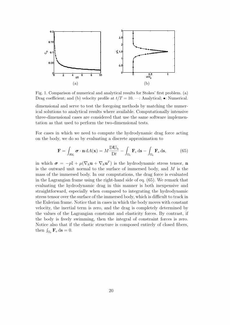
Fig. 1. Comparison of numerical and analytical results for Stokes’ first problem. (a)Drag coefficient; and (b) velocity profile at t/T = 10. —: Analytical; •: Numerical.

dimensional and serve to test the foregoing methods by matching the numer-ical solutions to analytical results where available. Computationally intensivethree-dimensional cases are considered that use the same software implemen-tation as that used to perform the two-dimensional tests.

For cases in which we need to compute the hydrodynamic drag force actingon the body, we do so by evaluating a discrete approximation to

F =∫

∂Uc

σ · n dA(x) = MDUb

Dt−∫Ωc

Fc ds−∫Ωe

Fe ds, (65)

in which σ = −pI + µ(∇hu + ∇huT ) is the hydrodynamic stress tensor, n

is the outward unit normal to the surface of immersed body, and M is themass of the immersed body. In our computations, the drag force is evaluatedin the Lagrangian frame using the right-hand side of eq. (65). We remark thatevaluating the hydrodynamic drag in this manner is both inexpensive andstraightforward, especially when compared to integrating the hydrodynamicstress tensor over the surface of the immersed body, which is difficult to track inthe Eulerian frame. Notice that in cases in which the body moves with constantvelocity, the inertial term is zero, and the drag is completely determined bythe values of the Lagrangian constraint and elasticity forces. By contrast, ifthe body is freely swimming, then the integral of constraint forces is zero.Notice also that if the elastic structure is composed entirely of closed fibers,then

∫Ωe

Fe ds = 0.

20

7.1 Prescribed motion

7.1.1 Stokes’ first problem

Our first example considers Stokes’ first problem, in which an infinitely longhorizontal plate is impulsively started with a velocity U0 in the x direction.The exact analytical solution for the transient velocity profile for y ≥ 0 isgiven by

u(y, t) = U0

[erfc

(y

2√

νt

)], (66)

in which ν = µ/ρ is the kinematic viscosity of the fluid. The drag coefficientis CD = F/1

2ρU2

0 A, in which F is the hydrodynamic drag force acting on onesurface of the plate and A is the area per unit depth of that surface. CD is givenanalytically by CD = 2√

πtRe, in which the Reynolds number is Re = U0L/ν.

This problem has been studied numerically by Shirgaonkar et al. [14] and byTaira and Colonius [63].

Here, we set U0 = 1, L = 1, and Re = 500. The time scale is T = L/U0. Thephysical domain U is taken to be a periodic region of size 3L×3L. To discretizeU , we use a four-level Cartesian grid, with the coarsest level consisting of auniform 32× 32 grid, and with refinement ratios n0

ref = n1ref = 4 and n2

ref = 2,so that the finest level of the hierarchy has a grid spacing equivalent to auniform 1024 × 1024 grid. The plate is modeled as a line of points placed inthe middle of U , and the discretization of the plate uses one material pointin per Cartesian grid cell and was kept on the finest grid level to resolvecompletely the viscous boundary layer. Fig. 1 shows comparisons between ournumerical results and the analytic solution. We obtain excellent agreementwith the analytical solution to this problem.

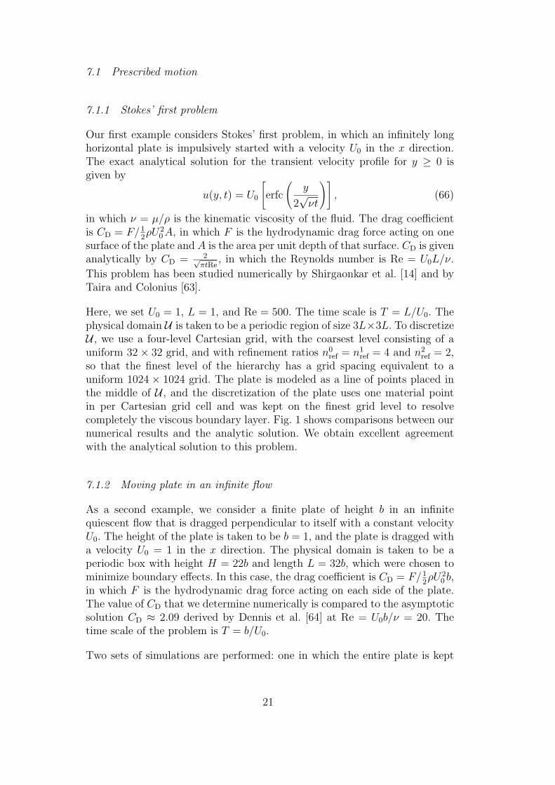
7.1.2 Moving plate in an infinite flow

As a second example, we consider a finite plate of height b in an infinitequiescent flow that is dragged perpendicular to itself with a constant velocityU0. The height of the plate is taken to be b = 1, and the plate is dragged witha velocity U0 = 1 in the x direction. The physical domain is taken to be aperiodic box with height H = 22b and length L = 32b, which were chosen tominimize boundary effects. In this case, the drag coefficient is CD = F/1

2ρU2

0 b,in which F is the hydrodynamic drag force acting on each side of the plate.The value of CD that we determine numerically is compared to the asymptoticsolution CD ≈ 2.09 derived by Dennis et al. [64] at Re = U0b/ν = 20. Thetime scale of the problem is T = b/U0.

Two sets of simulations are performed: one in which the entire plate is kept

21

(a)

(b)

Fig. 2. (a) Drag coefficient for a plate moving perpendicular to itself as a functionof nondimensionalized time at Re = 20. — (blue): Numerical, plate on single level;---: Numerical, plate spanning two adjacent grid levels; •: asymptotic value fromDennis et al. [64]. (b) A visualization of the second case considered, in which theupper half of the plate is on the finest grid level, and the lower half is on the nextcoarser level of the grid hierarchy.

on the finest level of the Cartesian grid hierarchy, and one in which half of theplate is kept on the finest level and the other half is kept on the next coarserlevel of the grid; see Fig. 2(b). For the first case, three grid levels are used, withthe coarsest level being a uniform 64×64 grid, and with a uniform refinementratio nref = 4. For the second case, one further grid level is introduced in thegrid hierarchy with a refinement ratio of n2

ref = 2. This second case is doneto validate the method for use with immersed structures that span multiplelevels of the Cartesian grid hierarchy. In both cases, the plate is modeled as aone dimensional line of points with one material point in each Cartesian gridcell.

Fig. 2 shows the time evolution of drag for the moving plate for the two cases,which are shown to agree well with the asymptotic value derived by Denniset al. [64]. Previous work has attributed the spurious oscillations observed inthe calculated drag coefficient to the IB formulation of the problem [14, 65].To filter these spurious high frequency oscillations, we report values that havebeen averaged over four consecutive time steps.

22

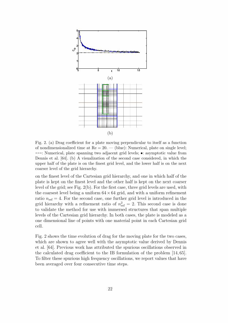
Table 1Comparison of mean drag coefficients and Strouhal numbers for various studies offlow past a rigid circular cylinder at Re = 200.

Study CD St

Present 1.3906 0.2000

Present (simplified velocity correction) 1.4001 0.2000

Braza et al. [66] 1.4000 0.2000

Henderson [67] 1.3412 0.1971

He et al. [68] 1.3560 0.1978

Bergmann et al. [27] 1.3500 0.1980

7.1.3 Flow past a rigid cylinder

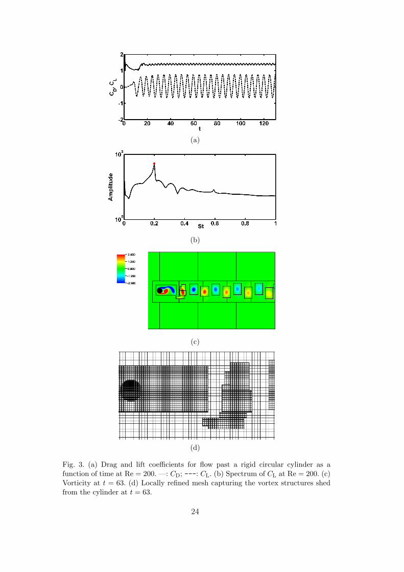
As a next example, we consider the widely used benchmark problem of flowpast a rigid circular cylinder. A circular cylinder of diameter D = 1 is placedin a flow with far-field velocity U∞. In this case, we determine the Reynoldsnumber as Re = ‖U∞‖D/ν = 200. We set U∞ = (1, 0). The computationaldomain is taken to be a rectangular channel U = [−8D, 24D] × [−8D, 8D],and the center of the cylinder is placed at (x, y) = (0, 0). The coarsest levelof the Eulerian discretization is a uniform 64× 32 grid, and a uniform refine-ment ratio nref = 4 is used to construct the finer levels of the patch hierarchy.The aerodynamic drag coefficient, C = F/(ρD‖U∞‖2/2), is calculated numer-ically. Drag and lift coefficients are defined as CD = C · ex and CL = C · ey,respectively.

Fig. 3(a) shows the temporal evolution of CD and CL as functions of time. Inthe figure, time has been normalized by D/‖U∞‖. To remove spurious oscil-lations in the computed drag and lift forces, we filter the drag and lift coeffi-cients by averaging values over five consecutive time steps. Table 1 comparesthe mean drag coefficient and Strouhal number computed using the presentmethod at Re = 200 to corresponding values obtained in previous studies.Good agreement is demonstrated between our results and results from theseprior investigations. Table 1 also shows that for this problem, including a finaldivergence-free projection is not required to obtain accurate results for thedrag coefficient and Strouhal number; see Sec. 4.1. In particular, notice thatessentially identical dynamics, as quantified by St, are recovered both with thefinal divergence-free projection and also with the simplified velocity correctionthat omits the final projection. The reason that omitting this projection hasa small effect on the computed dynamics is that the flow field is effectivelyprojected in the first solution step of the subsequent time step. Fig. 4 shows∇ · u for the two cases considered above. As can be seen in Fig. 4(a), the ve-

23

(a)

(b)

(c)

(d)

Fig. 3. (a) Drag and lift coefficients for flow past a rigid circular cylinder as afunction of time at Re = 200. —: CD; ---: CL. (b) Spectrum of CL at Re = 200. (c)Vorticity at t = 63. (d) Locally refined mesh capturing the vortex structures shedfrom the cylinder at t = 63.

24

(a)

(b)

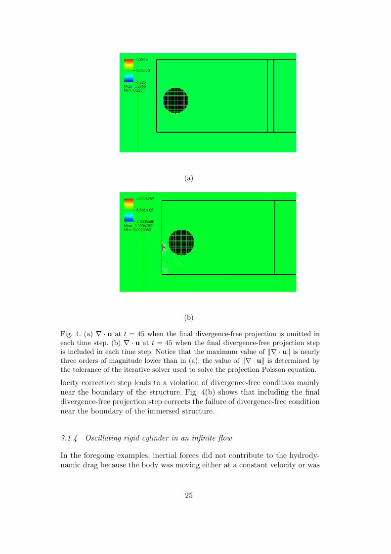
Fig. 4. (a) ∇ · u at t = 45 when the final divergence-free projection is omitted ineach time step. (b) ∇ · u at t = 45 when the final divergence-free projection stepis included in each time step. Notice that the maximum value of ‖∇ · u‖ is nearlythree orders of magnitude lower than in (a); the value of ‖∇ · u‖ is determined bythe tolerance of the iterative solver used to solve the projection Poisson equation.

locity correction step leads to a violation of divergence-free condition mainlynear the boundary of the structure. Fig. 4(b) shows that including the finaldivergence-free projection step corrects the failure of divergence-free conditionnear the boundary of the immersed structure.

7.1.4 Oscillating rigid cylinder in an infinite flow

In the foregoing examples, inertial forces did not contribute to the hydrody-namic drag because the body was moving either at a constant velocity or was

25

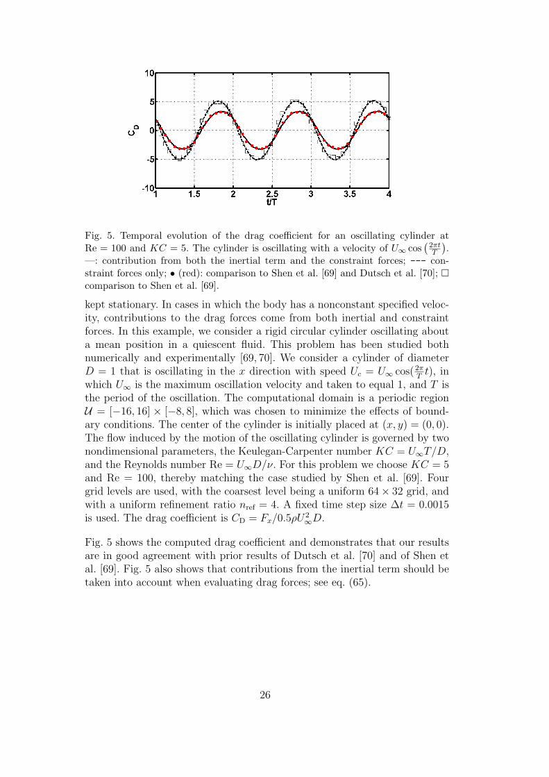
Fig. 5. Temporal evolution of the drag coefficient for an oscillating cylinder atRe = 100 and KC = 5. The cylinder is oscillating with a velocity of U∞ cos

(2πtT

).

—: contribution from both the inertial term and the constraint forces; --- con-straint forces only; • (red): comparison to Shen et al. [69] and Dutsch et al. [70]; comparison to Shen et al. [69].

kept stationary. In cases in which the body has a nonconstant specified veloc-ity, contributions to the drag forces come from both inertial and constraintforces. In this example, we consider a rigid circular cylinder oscillating abouta mean position in a quiescent fluid. This problem has been studied bothnumerically and experimentally [69, 70]. We consider a cylinder of diameterD = 1 that is oscillating in the x direction with speed Uc = U∞ cos(2π

Tt), in

which U∞ is the maximum oscillation velocity and taken to equal 1, and T isthe period of the oscillation. The computational domain is a periodic regionU = [−16, 16] × [−8, 8], which was chosen to minimize the effects of bound-ary conditions. The center of the cylinder is initially placed at (x, y) = (0, 0).The flow induced by the motion of the oscillating cylinder is governed by twonondimensional parameters, the Keulegan-Carpenter number KC = U∞T/D,and the Reynolds number Re = U∞D/ν. For this problem we choose KC = 5and Re = 100, thereby matching the case studied by Shen et al. [69]. Fourgrid levels are used, with the coarsest level being a uniform 64× 32 grid, andwith a uniform refinement ratio nref = 4. A fixed time step size ∆t = 0.0015is used. The drag coefficient is CD = Fx/0.5ρU2

∞D.

Fig. 5 shows the computed drag coefficient and demonstrates that our resultsare in good agreement with prior results of Dutsch et al. [70] and of Shen etal. [69]. Fig. 5 also shows that contributions from the inertial term should betaken into account when evaluating drag forces; see eq. (65).

26

(a)

(b) (c)

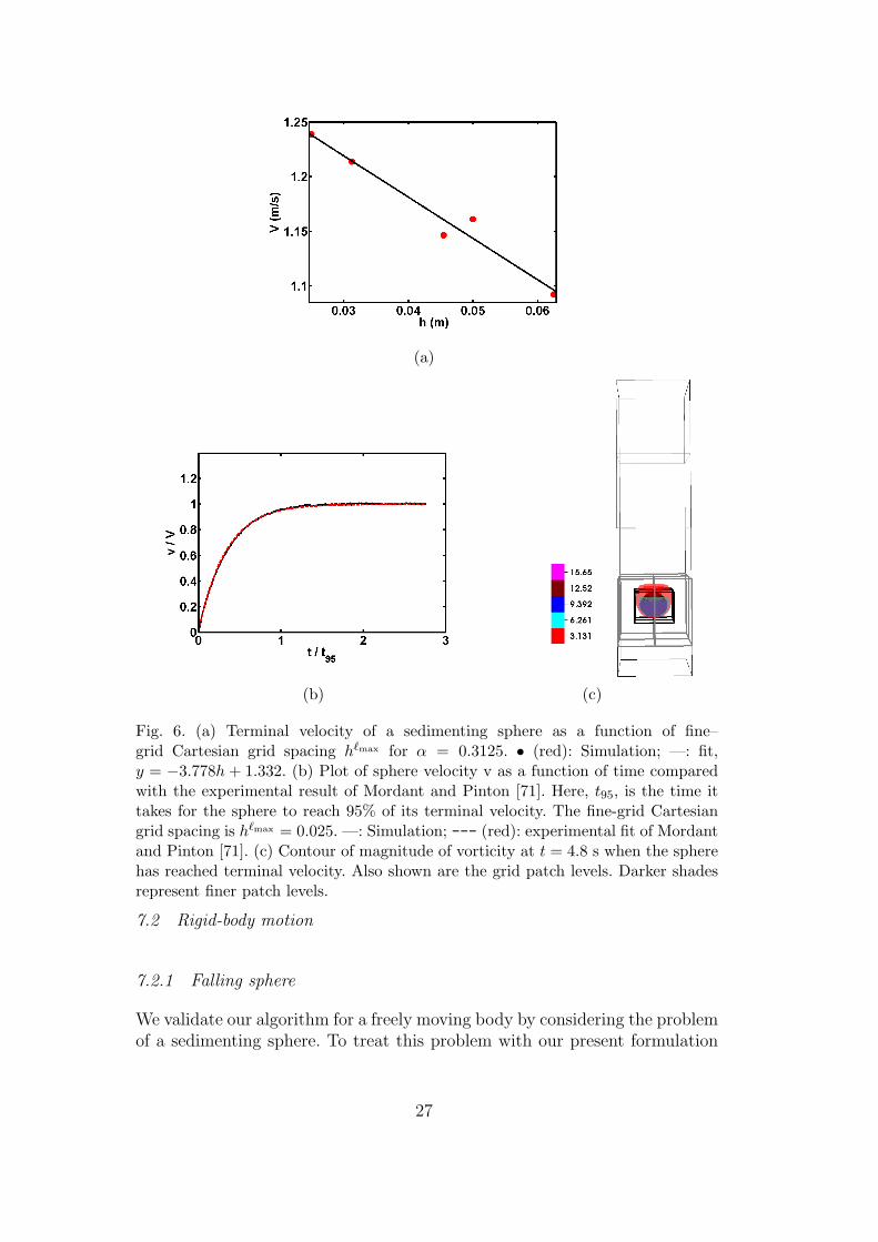
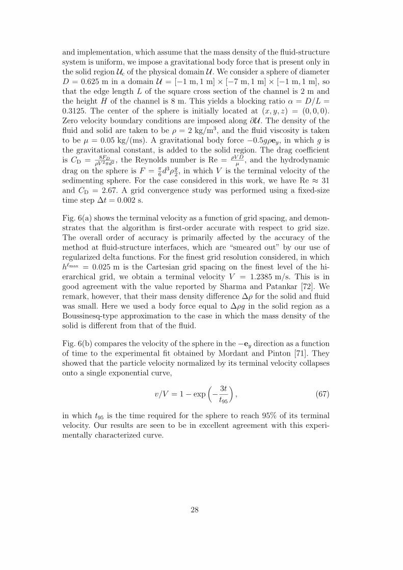
Fig. 6. (a) Terminal velocity of a sedimenting sphere as a function of fine–grid Cartesian grid spacing h`max for α = 0.3125. • (red): Simulation; —: fit,y = −3.778h + 1.332. (b) Plot of sphere velocity v as a function of time comparedwith the experimental result of Mordant and Pinton [71]. Here, t95, is the time ittakes for the sphere to reach 95% of its terminal velocity. The fine-grid Cartesiangrid spacing is h`max = 0.025. —: Simulation; --- (red): experimental fit of Mordantand Pinton [71]. (c) Contour of magnitude of vorticity at t = 4.8 s when the spherehas reached terminal velocity. Also shown are the grid patch levels. Darker shadesrepresent finer patch levels.

7.2 Rigid-body motion

7.2.1 Falling sphere

We validate our algorithm for a freely moving body by considering the problemof a sedimenting sphere. To treat this problem with our present formulation

27

and implementation, which assume that the mass density of the fluid-structuresystem is uniform, we impose a gravitational body force that is present only inthe solid region Uc of the physical domain U . We consider a sphere of diameterD = 0.625 m in a domain U = [−1 m, 1 m] × [−7 m, 1 m] × [−1 m, 1 m], sothat the edge length L of the square cross section of the channel is 2 m andthe height H of the channel is 8 m. This yields a blocking ratio α = D/L =0.3125. The center of the sphere is initially located at (x, y, z) = (0, 0, 0).Zero velocity boundary conditions are imposed along ∂U . The density of thefluid and solid are taken to be ρ = 2 kg/m3, and the fluid viscosity is takento be µ = 0.05 kg/(ms). A gravitational body force −0.5gρey, in which g isthe gravitational constant, is added to the solid region. The drag coefficientis CD = 8FD

ρV 2πd2 , the Reynolds number is Re = ρV Dµ

, and the hydrodynamic

drag on the sphere is F = π6d3ρg

2, in which V is the terminal velocity of the

sedimenting sphere. For the case considered in this work, we have Re ≈ 31and CD = 2.67. A grid convergence study was performed using a fixed-sizetime step ∆t = 0.002 s.

Fig. 6(a) shows the terminal velocity as a function of grid spacing, and demon-strates that the algorithm is first-order accurate with respect to grid size.The overall order of accuracy is primarily affected by the accuracy of themethod at fluid-structure interfaces, which are “smeared out” by our use ofregularized delta functions. For the finest grid resolution considered, in whichh`max = 0.025 m is the Cartesian grid spacing on the finest level of the hi-erarchical grid, we obtain a terminal velocity V = 1.2385 m/s. This is ingood agreement with the value reported by Sharma and Patankar [72]. Weremark, however, that their mass density difference ∆ρ for the solid and fluidwas small. Here we used a body force equal to ∆ρg in the solid region as aBoussinesq-type approximation to the case in which the mass density of thesolid is different from that of the fluid.

Fig. 6(b) compares the velocity of the sphere in the −ey direction as a functionof time to the experimental fit obtained by Mordant and Pinton [71]. Theyshowed that the particle velocity normalized by its terminal velocity collapsesonto a single exponential curve,

v/V = 1− exp(− 3t

t95

), (67)

in which t95 is the time required for the sphere to reach 95% of its terminalvelocity. Our results are seen to be in excellent agreement with this experi-mentally characterized curve.

28

7.2.2 Impulsively started cylinder

We take the case of impulsively started cylinder in a quiescent flow to demon-strate the momentum-conservation properties of our method. A cylinder of di-ameter D = 1 m is placed the center of a periodic domain of size [32 m×16 m]at time t = 0. An impulse of the form I(t) = 400 exp(−400t) N/m−3 is appliedin the x direction in within the body, at its initial position, thereby impul-sively starting its motion. The net momentum ∆Mx imparted to the systemin the x direction is found analytically as

∆Mx =∫Ub(t=0)

∫ t=∞

t=0I(t) dt ds. (68)

The density of fluid and solid is set to 1 kg/m−3, and the Reynolds numberRe = ρV D

µis taken to be 200 with the reference velocity V = 1 m/s. Three

grid levels are used in the simulation, with the coarsest grid having 64 × 32grid cells. A uniform refinement ratio nref = 4 is used for subsequent patchlevels.

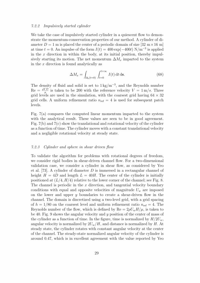
Fig. 7(a) compares the computed linear momentum imparted to the systemwith the analytical result. These values are seen to be in good agreement.Fig. 7(b) and 7(c) show the translational and rotational velocity of the cylinderas a function of time. The cylinder moves with a constant translational velocityand a negligible rotational velocity at steady state.

7.2.3 Cylinder and sphere in shear driven flow

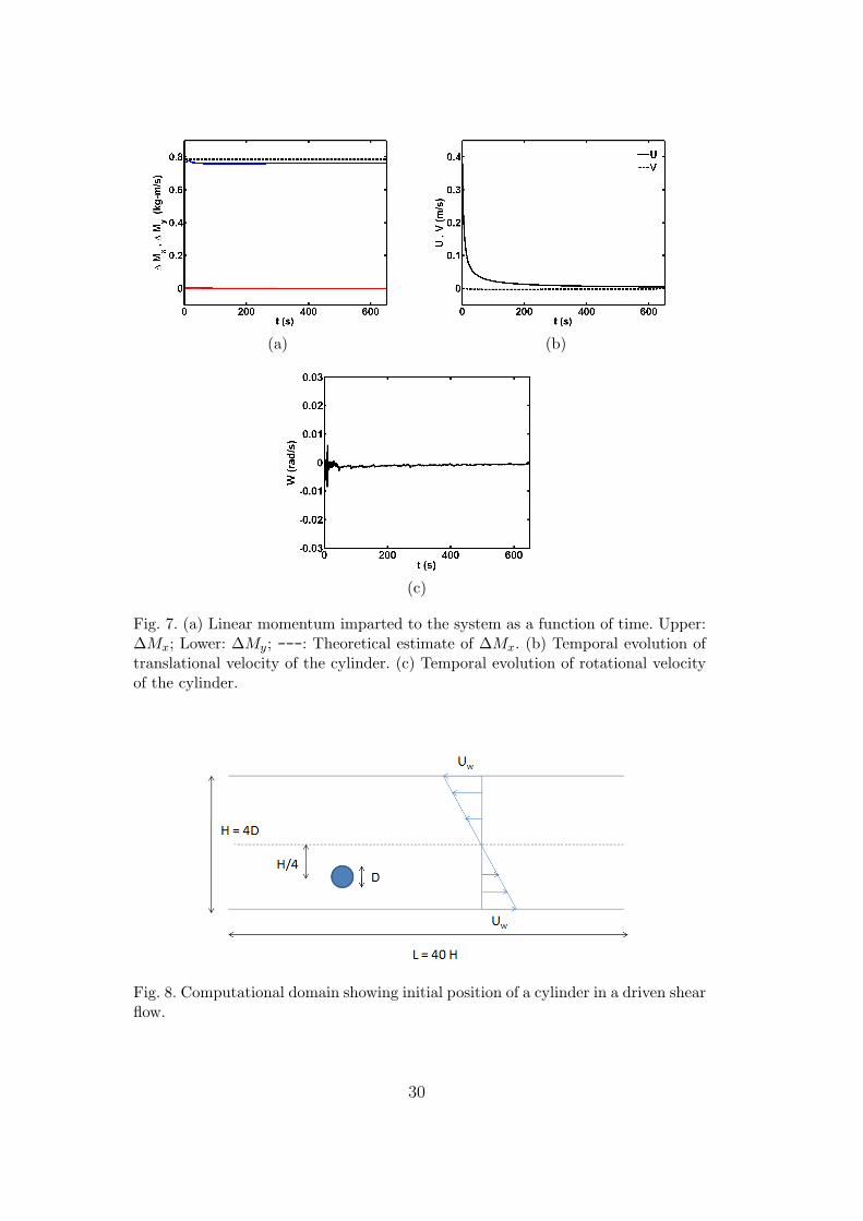
To validate the algorithm for problems with rotational degrees of freedom,we consider rigid bodies in shear-driven channel flow. For a two-dimensionalvalidation case, we consider a cylinder in shear flow, as considered by Yeoet al. [73]. A cylinder of diameter D is immersed in a rectangular channel ofheight H = 4D and length L = 40H. The center of the cylinder is initiallypositioned at (L/4, H/4) relative to the lower corner of the channel; see Fig. 8.The channel is periodic in the x direction, and tangential velocity boundaryconditions with equal and opposite velocities of magnitude Uw are imposedon the lower and upper y boundaries to create a shear-driven flow in thechannel. The domain is discretized using a two-level grid, with a grid spacingof h = 1/80 on the coarsest level and uniform refinement ratio nref = 4. TheReynolds number of the flow, which is defined by Re = 2ρUwH/µ, is taken tobe 40. Fig. 9 shows the angular velocity and y position of the center of mass ofthe cylinder as a function of time. In the figure, time is normalized by H/2Uw,angular velocity is normalized by 2Uw/H, and distance is normalized by H. Atsteady state, the cylinder rotates with constant angular velocity at the centerof the channel. The steady-state normalized angular velocity of the cylinder isaround 0.47, which is in excellent agreement with the value reported by Yeo

29

(a) (b)

(c)

Fig. 7. (a) Linear momentum imparted to the system as a function of time. Upper:∆Mx; Lower: ∆My; ---: Theoretical estimate of ∆Mx. (b) Temporal evolution oftranslational velocity of the cylinder. (c) Temporal evolution of rotational velocityof the cylinder.

Fig. 8. Computational domain showing initial position of a cylinder in a driven shearflow.

30

(a) (b)

Fig. 9. Cylinder in a shear flow at Re = 40. (a) Normalized angular velocity of thecylinder as a function of time. (b) y position of the center of mass of the cylinderas a function of time.

Fig. 10. Time evolution of normalized angular velocity of a sphere in a driven shearflow as a function of time for shear rates γ = 1/s and 3/s. In the cases consideredhere, Re = 10.

et al. [73].

Next, we consider the three-dimensional case of a neutrally bouyant spherein a shear-driven channel flow. This problem has been experimentally andnumerically studied in previous work [74–78]. A sphere of radius R is immersedin a rectangular channel of width 40R, and with height and breadth of 6R. Thesphere is positioned at the center of the channel, and the walls of the channelare moved at a velocity of −γy in x direction to create a flow with shear rateγ. The physical domain is discretized by a two-level grid, with the coarse levelconsisting of a uniform 200 × 30 × 30 grid, and with a refinement ratio ofnref = 4 between levels. The Reynolds number of the flow is Re = ργR2/µ andis set to equal 10. Fig. 10 shows the angular velocity of the sphere (normalizedby γ) as a function of time (normalized by 1/γ) for shear rates γ = 1/s and3/s. Both curves collapse on each other. Steady state is achieved earlier athigher shear rate. The steady state angular velocity of the sphere reaches a

31

value of 0.4. This is in excellent agreement with the study done by Mikulencakand Morris [77].

7.3 Free swimming

We next consider problems involving free swimming in which the body is re-quired to move with a prescribed kinematic velocity or shape. In these cases,although the deformational kinematics of the body are prescribed, it is im-portant to note that the translational and rotational velocities of the bodyare not specified in advance; rather, they are determined by the interactionof the immersed body and the fluid. We use two models, a two-dimensionalmodel of a freely swimming eel with kinematics that are imposed using theprescribed-shape method described in Sec. 4.4, and a three-dimensional modelof the black ghost knifefish, for which we use the prescribed-kinematic velocitymethods described in Sec. 4.3.

7.3.1 Two-dimensional model of eel swimming

As an initial example, we consider a two-dimensional model of eel swim-ming [2, 14]. The geometry and deformation of the eel body is prescribedanalytically, as described below, and a periodic backward-traveling wave ispassed over the body to induce forward swimming. We use the prescribed-shape approach described in Sec. 4.4 to update the position of the body,and we verify that “filtered” and “unfiltered” prescribed shape mappings (seeSec. 4.4) yield identical results.

The geometry of the eel body is given in a reference configuration that isaligned with the x-coordinate axis. This geometry is specified in terms of thevertical displacement y(x, t) of the midline of the eel body from the x-axis,and in terms of the width w(x) of a body cross-section perpendicular to thex-axis at each point 0 ≤ x ≤ L along the projected length L of the eel. Toaccount for the traveling wave, the displacement of the midline from the x-axisis given by

y(x, t) = 0.125x + 0.03125

1.03125sin [2π(x− t/T )] , (69)

for 0 ≤ x ≤ L, in which T is the time period of a backward-traveling wave.The width of a body cross-section perpendicular to the x-axis and centeredabout the midline of the body is given by

w(x) =

√

2wHx− x2 for 0 ≤ x < xH,

wHL−x

L−xHfor xH ≤ x < L,

(70)

in which wH = 0.04L is the width of the eel at its “head,” which is located at

32

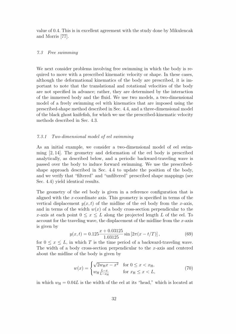
(a) (b)

Fig. 11. (a) Temporal evolution of different translational velocities induced by theunfiltered kinematics. —: Projected axial velocity, Up; ---: Projected lateral veloc-ity, Vp; — (red): Net axial velocity of deformational kinematics, Up,k; -N- (cyan):Net lateral velocity of deformational kinematics, Vp,k. (b) Temporal evolution ofrotational velocities induced by the unfiltered kinematics. —: Projected W z

p ; ---:Net W z

p,k of the deformational kinematics.

xH = wH. Time is normalized by T , distances are normalized by L, masses arenormalized by the mass of eel and velocities are normalized by U0 = L/T = 1.The Reynolds number of the flow is Re = VmaxL/ν = 5609, in which Vmax =0.785 U0 is the maximum undulatory velocity at the tail tip.

We use a periodic computational domain of size 8L× 4L. We employ a four-level Cartesian grid with the coarsest level having 32×16 grid cells. A uniformrefinement ratio nref = 4 is used for subsequent patch levels. To resolve theboundary layer along the fluid-body interface, the body is always kept withinthe finest grid level. Grid cells are also tagged for refinement wherever ‖ωz‖ ≥0.25 on level 0, ‖ωz‖ ≥ 0.5 on level 1, ‖ωz‖ ≥ 1 on level 2, and ‖ωz‖ ≥ 2 onlevel 3.

Because we have an analytic formula for the body shape, the deformationalvelocity can be obtained by differentiating the prescribed shape with respectto t. Specifically, it is not necessary to use finite differencing or other numer-ical approximation techniques to obtain Uk. We remark, however, that thedeformational kinematic velocity obtained from the analytic formulae for thebody shape has nonzero net translational and rotational velocities, and thesenet velocities should not be imposed on the motion. We perform two setsof simulations: one in which the prescribed shape and deformational velocityare obtained from a filtered shape mapping, in which the net translationaland rotational motions have been removed from the prescribed shape andkinematic velocity, and the other using the unfiltered shape and kinematicvelocity obtained from the analytic formulae for the body shape. Because themethod described in Sec. 4.4 corrects for any net linear or angular velocityin the prescribed shape, both cases should yield the same numerical results.

33

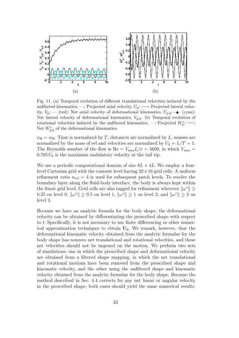
(a) (b)

Fig. 12. (a) Temporal evolution of translational velocities induced by the filteredkinematics. Upper: Rigid axial velocity of the center of mass. Lower: Rigid lateralvelocity of the center of mass. —: Rigid translational velocity induced by the fil-tered kinematics, Ur; • (red) Validation of eq. (56) when unfiltered kinematics areused. (b) Temporal evolution of rotational velocity of center of mass of the eel in-duced by the filtered kinematics. —: Rigid rotational velocity induced by the filteredkinematics, W z

r ; • (red) Validation of eq. (57) when unfiltered kinematics are used.

(a) t = 4 (b) t = 5.5

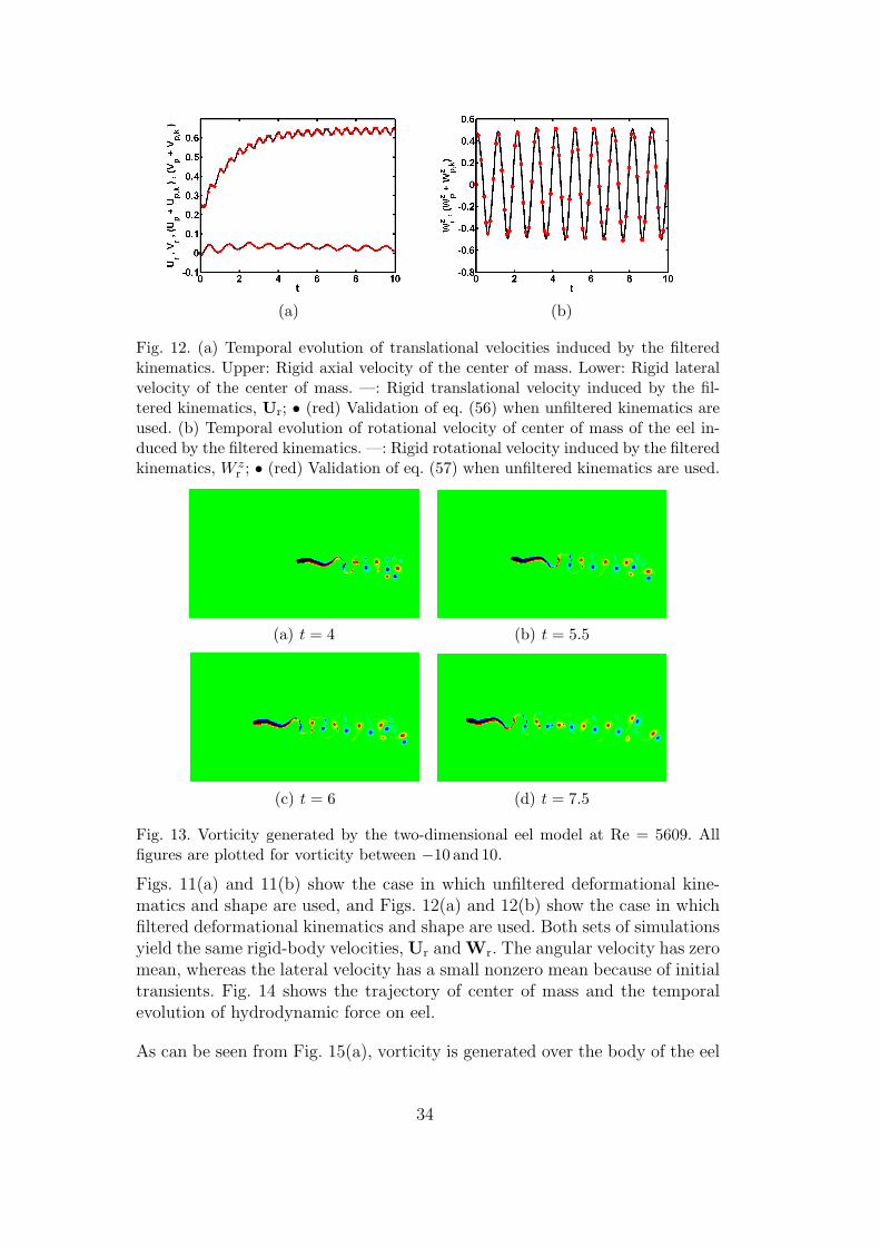
(c) t = 6 (d) t = 7.5

Fig. 13. Vorticity generated by the two-dimensional eel model at Re = 5609. Allfigures are plotted for vorticity between −10 and 10.

Figs. 11(a) and 11(b) show the case in which unfiltered deformational kine-matics and shape are used, and Figs. 12(a) and 12(b) show the case in whichfiltered deformational kinematics and shape are used. Both sets of simulationsyield the same rigid-body velocities, Ur and Wr. The angular velocity has zeromean, whereas the lateral velocity has a small nonzero mean because of initialtransients. Fig. 14 shows the trajectory of center of mass and the temporalevolution of hydrodynamic force on eel.

As can be seen from Fig. 15(a), vorticity is generated over the body of the eel

34

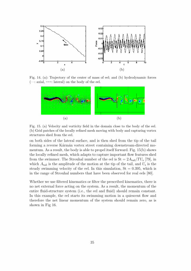
(a) (b)

Fig. 14. (a): Trajectory of the center of mass of eel; and (b) hydrodynamic forces(—: axial, ---: lateral) on the body of the eel.

(a) (b)

Fig. 15. (a) Velocity and vorticity field in the domain close to the body of the eel.(b) Grid patches of the locally refined mesh moving with body and capturing vortexstructures shed from the eel.

on both sides of the lateral surface, and is then shed from the tip of the tailforming a reverse Karman vortex street containing downstream-directed mo-mentum. As a result, the body is able to propel itself forward. Fig. 15(b) showsthe locally refined mesh, which adapts to capture important flow features shedfrom the swimmer. The Strouhal number of the eel is St = 2Atail/TUs [79], inwhich Atail is the amplitude of the motion at the tip of the tail, and Us is thesteady swimming velocity of the eel. In this simulation, St = 0.395, which isin the range of Strouhal numbers that have been observed for real eels [80].

Whether we use filtered kinematics or filter the prescribed kinematics, there isno net external force acting on the system. As a result, the momentum of theentire fluid-structure system (i.e., the eel and fluid) should remain constant.In this example, the eel starts its swimming motion in a quiescent flow andtherefore the net linear momentum of the system should remain zero, as isshown in Fig 16.

35

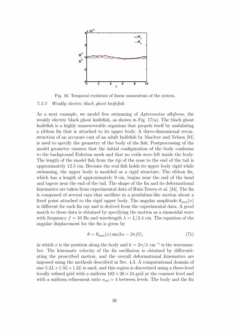
Fig. 16. Temporal evolution of linear momentum of the system.

7.3.2 Weakly electric black ghost knifefish

As a next example, we model free swimming of Apteronotus albifrons, theweakly electric black ghost knifefish, as shown in Fig. 17(a). The black ghostknifefish is a highly maneuverable organism that propels itself by undulatinga ribbon fin that is attached to its upper body. A three-dimensional recon-struction of an accurate cast of an adult knifefish by MacIver and Nelson [81]is used to specify the geometry of the body of the fish. Postprocessing of themodel geometry ensures that the initial configuration of the body conformsto the background Eulerian mesh and that no voids were left inside the body.The length of the model fish from the tip of the nose to the end of the tail isapproximately 12.5 cm. Because the real fish holds its upper body rigid whileswimming, the upper body is modeled as a rigid structure. The ribbon fin,which has a length of approximately 9 cm, begins near the end of the headand tapers near the end of the tail. The shape of the fin and its deformationalkinematics are taken from experimental data of Ruiz-Torres et al. [34]. The finis composed of several rays that oscillate in a pendulum-like motion about afixed point attached to the rigid upper body. The angular amplitude θmax(x)is different for each fin ray and is derived from the experimental data. A goodmatch to these data is obtained by specifying the motion as a sinusoidal wavewith frequency f = 10 Hz and wavelength λ = L/2.4 cm. The equation of theangular displacement for the fin is given by

θ = θmax(x) sin(kx− 2πft), (71)

in which x is the position along the body and k = 2π/λ cm−1 is the wavenum-ber. The kinematic velocity of the fin oscillation is obtained by differenti-ating the prescribed motion, and the overall deformational kinematics areimposed using the methods described in Sec. 4.3. A computational domain ofsize 5.2L×1.3L×1.2L is used, and this region is discretized using a three-levellocally refined grid with a uniform 102× 26× 24 grid at the coarsest level andwith a uniform refinement ratio nref = 4 between levels. The body and the fin

36

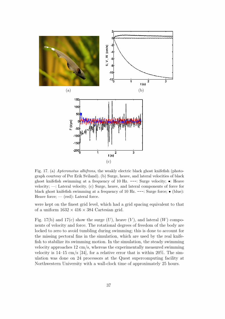
(a) (b)

(c)

Fig. 17. (a) Apteronotus albifrons, the weakly electric black ghost knifefish (photo-graph courtesy of Per Erik Sviland). (b) Surge, heave, and lateral velocities of blackghost knifefish swimming at a frequency of 10 Hz. ---: Surge velocity; •: Heavevelocity; —: Lateral velocity. (c) Surge, heave, and lateral components of force forblack ghost knifefish swimming at a frequency of 10 Hz. ---: Surge force; • (blue):Heave force; — (red): Lateral force.

were kept on the finest grid level, which had a grid spacing equivalent to thatof a uniform 1632× 416× 384 Cartesian grid.

Fig. 17(b) and 17(c) show the surge (U), heave (V ), and lateral (W ) compo-nents of velocity and force. The rotational degrees of freedom of the body arelocked to zero to avoid tumbling during swimming; this is done to account forthe missing pectoral fins in the simulation, which are used by the real knife-fish to stabilize its swimming motion. In the simulation, the steady swimmingvelocity approaches 12 cm/s, whereas the experimentally measured swimmingvelocity is 14–15 cm/s [34], for a relative error that is within 20%. The sim-ulation was done on 24 processors at the Quest supercomputing facility atNorthwestern University with a wall-clock time of approximately 25 hours.

37

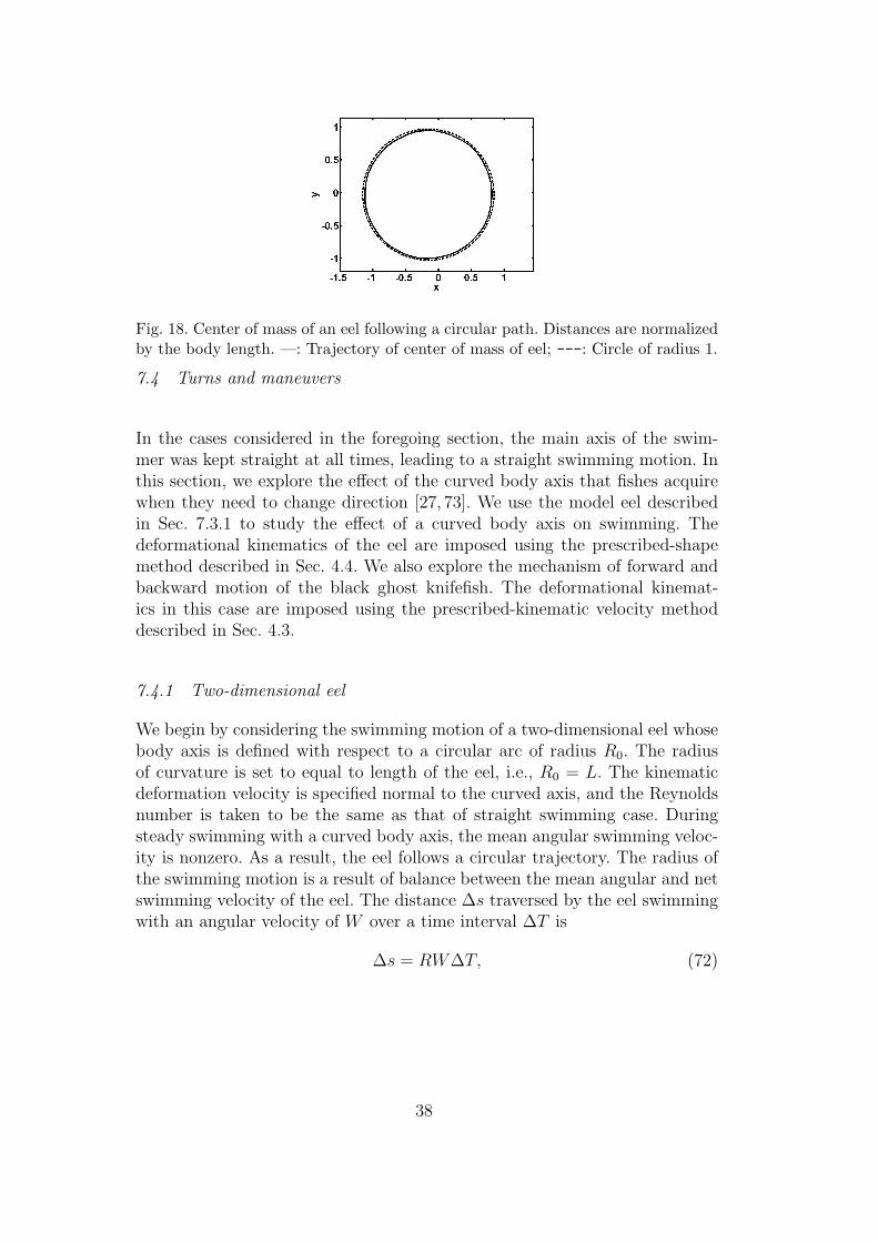
Fig. 18. Center of mass of an eel following a circular path. Distances are normalizedby the body length. —: Trajectory of center of mass of eel; ---: Circle of radius 1.

7.4 Turns and maneuvers

In the cases considered in the foregoing section, the main axis of the swim-mer was kept straight at all times, leading to a straight swimming motion. Inthis section, we explore the effect of the curved body axis that fishes acquirewhen they need to change direction [27, 73]. We use the model eel describedin Sec. 7.3.1 to study the effect of a curved body axis on swimming. Thedeformational kinematics of the eel are imposed using the prescribed-shapemethod described in Sec. 4.4. We also explore the mechanism of forward andbackward motion of the black ghost knifefish. The deformational kinemat-ics in this case are imposed using the prescribed-kinematic velocity methoddescribed in Sec. 4.3.

7.4.1 Two-dimensional eel

We begin by considering the swimming motion of a two-dimensional eel whosebody axis is defined with respect to a circular arc of radius R0. The radiusof curvature is set to equal to length of the eel, i.e., R0 = L. The kinematicdeformation velocity is specified normal to the curved axis, and the Reynoldsnumber is taken to be the same as that of straight swimming case. Duringsteady swimming with a curved body axis, the mean angular swimming veloc-ity is nonzero. As a result, the eel follows a circular trajectory. The radius ofthe swimming motion is a result of balance between the mean angular and netswimming velocity of the eel. The distance ∆s traversed by the eel swimmingwith an angular velocity of W over a time interval ∆T is

∆s = RW∆T, (72)

38

(a) t = 2 (b) t = 5

(c) t = 7.5 (d) t = 11

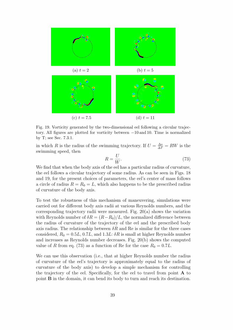
Fig. 19. Vorticity generated by the two-dimensional eel following a circular trajec-tory. All figures are plotted for vorticity between −10 and 10. Time is normalizedby T; see Sec. 7.3.1.

in which R is the radius of the swimming trajectory. If U = ∆s∆T

= RW is theswimming speed, then

R =U

W. (73)

We find that when the body axis of the eel has a particular radius of curvature,the eel follows a circular trajectory of some radius. As can be seen in Figs. 18and 19, for the present choices of parameters, the eel’s center of mass followsa circle of radius R = R0 = L, which also happens to be the prescribed radiusof curvature of the body axis.

To test the robustness of this mechanism of maneuvering, simulations werecarried out for different body axis radii at various Reynolds numbers, and thecorresponding trajectory radii were measured. Fig. 20(a) shows the variationwith Reynolds number of δR = (R−R0)/L, the normalized difference betweenthe radius of curvature of the trajectory of the eel and the prescribed bodyaxis radius. The relationship between δR and Re is similar for the three casesconsidered, R0 = 0.5L, 0.7L, and 1.3L: δR is small at higher Reynolds numberand increases as Reynolds number decreases. Fig. 20(b) shows the computedvalue of R from eq. (73) as a function of Re for the case R0 = 0.7L.

We can use this observation (i.e., that at higher Reynolds number the radiusof curvature of the eel’s trajectory is approximately equal to the radius ofcurvature of the body axis) to develop a simple mechanism for controllingthe trajectory of the eel. Specifically, for the eel to travel from point A topoint B in the domain, it can bend its body to turn and reach its destination.

39

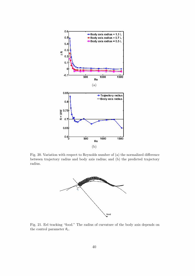
(a)

(b)

Fig. 20. Variation with respect to Reynolds number of (a) the normalized differencebetween trajectory radius and body axis radius; and (b) the predicted trajectoryradius.

Fig. 21. Eel tracking “food.” The radius of curvature of the body axis depends onthe control parameter θv.

40

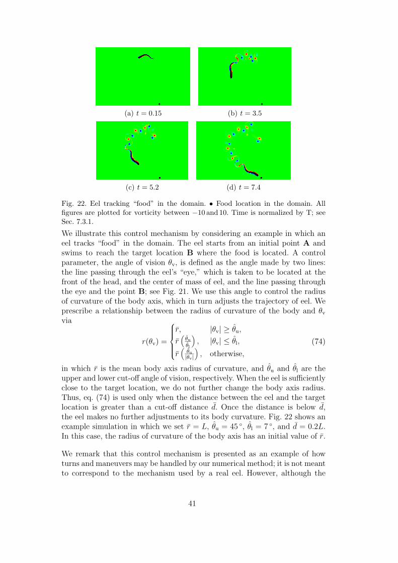
(a) t = 0.15 (b) t = 3.5

(c) t = 5.2 (d) t = 7.4

Fig. 22. Eel tracking “food” in the domain. • Food location in the domain. Allfigures are plotted for vorticity between −10 and 10. Time is normalized by T; seeSec. 7.3.1.

We illustrate this control mechanism by considering an example in which aneel tracks “food” in the domain. The eel starts from an initial point A andswims to reach the target location B where the food is located. A controlparameter, the angle of vision θv, is defined as the angle made by two lines:the line passing through the eel’s “eye,” which is taken to be located at thefront of the head, and the center of mass of eel, and the line passing throughthe eye and the point B; see Fig. 21. We use this angle to control the radiusof curvature of the body axis, which in turn adjusts the trajectory of eel. Weprescribe a relationship between the radius of curvature of the body and θv

via

r(θv) =

r, |θv| ≥ θu,

r(

θu

θl

), |θv| ≤ θl,

r(

θu

|θv|

), otherwise,

(74)

in which r is the mean body axis radius of curvature, and θu and θl are theupper and lower cut-off angle of vision, respectively. When the eel is sufficientlyclose to the target location, we do not further change the body axis radius.Thus, eq. (74) is used only when the distance between the eel and the targetlocation is greater than a cut-off distance d. Once the distance is below d,the eel makes no further adjustments to its body curvature. Fig. 22 shows anexample simulation in which we set r = L, θu = 45 , θl = 7 , and d = 0.2L.In this case, the radius of curvature of the body axis has an initial value of r.

We remark that this control mechanism is presented as an example of howturns and maneuvers may be handled by our numerical method; it is not meantto correspond to the mechanism used by a real eel. However, although the

41

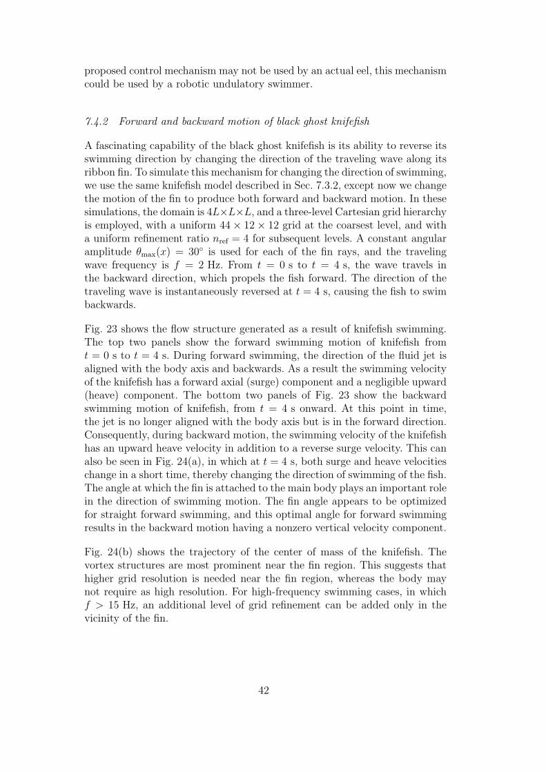
proposed control mechanism may not be used by an actual eel, this mechanismcould be used by a robotic undulatory swimmer.

7.4.2 Forward and backward motion of black ghost knifefish

A fascinating capability of the black ghost knifefish is its ability to reverse itsswimming direction by changing the direction of the traveling wave along itsribbon fin. To simulate this mechanism for changing the direction of swimming,we use the same knifefish model described in Sec. 7.3.2, except now we changethe motion of the fin to produce both forward and backward motion. In thesesimulations, the domain is 4L×L×L, and a three-level Cartesian grid hierarchyis employed, with a uniform 44× 12× 12 grid at the coarsest level, and witha uniform refinement ratio nref = 4 for subsequent levels. A constant angularamplitude θmax(x) = 30 is used for each of the fin rays, and the travelingwave frequency is f = 2 Hz. From t = 0 s to t = 4 s, the wave travels inthe backward direction, which propels the fish forward. The direction of thetraveling wave is instantaneously reversed at t = 4 s, causing the fish to swimbackwards.

Fig. 23 shows the flow structure generated as a result of knifefish swimming.The top two panels show the forward swimming motion of knifefish fromt = 0 s to t = 4 s. During forward swimming, the direction of the fluid jet isaligned with the body axis and backwards. As a result the swimming velocityof the knifefish has a forward axial (surge) component and a negligible upward(heave) component. The bottom two panels of Fig. 23 show the backwardswimming motion of knifefish, from t = 4 s onward. At this point in time,the jet is no longer aligned with the body axis but is in the forward direction.Consequently, during backward motion, the swimming velocity of the knifefishhas an upward heave velocity in addition to a reverse surge velocity. This canalso be seen in Fig. 24(a), in which at t = 4 s, both surge and heave velocitieschange in a short time, thereby changing the direction of swimming of the fish.The angle at which the fin is attached to the main body plays an important rolein the direction of swimming motion. The fin angle appears to be optimizedfor straight forward swimming, and this optimal angle for forward swimmingresults in the backward motion having a nonzero vertical velocity component.

Fig. 24(b) shows the trajectory of the center of mass of the knifefish. Thevortex structures are most prominent near the fin region. This suggests thathigher grid resolution is needed near the fin region, whereas the body maynot require as high resolution. For high-frequency swimming cases, in whichf > 15 Hz, an additional level of grid refinement can be added only in thevicinity of the fin.

42

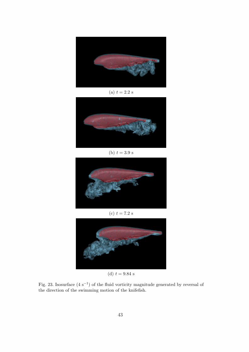
(a) t = 2.2 s

(b) t = 3.9 s

(c) t = 7.2 s

(d) t = 9.84 s

Fig. 23. Isosurface (4 s−1) of the fluid vorticity magnitude generated by reversal ofthe direction of the swimming motion of the knifefish.

43

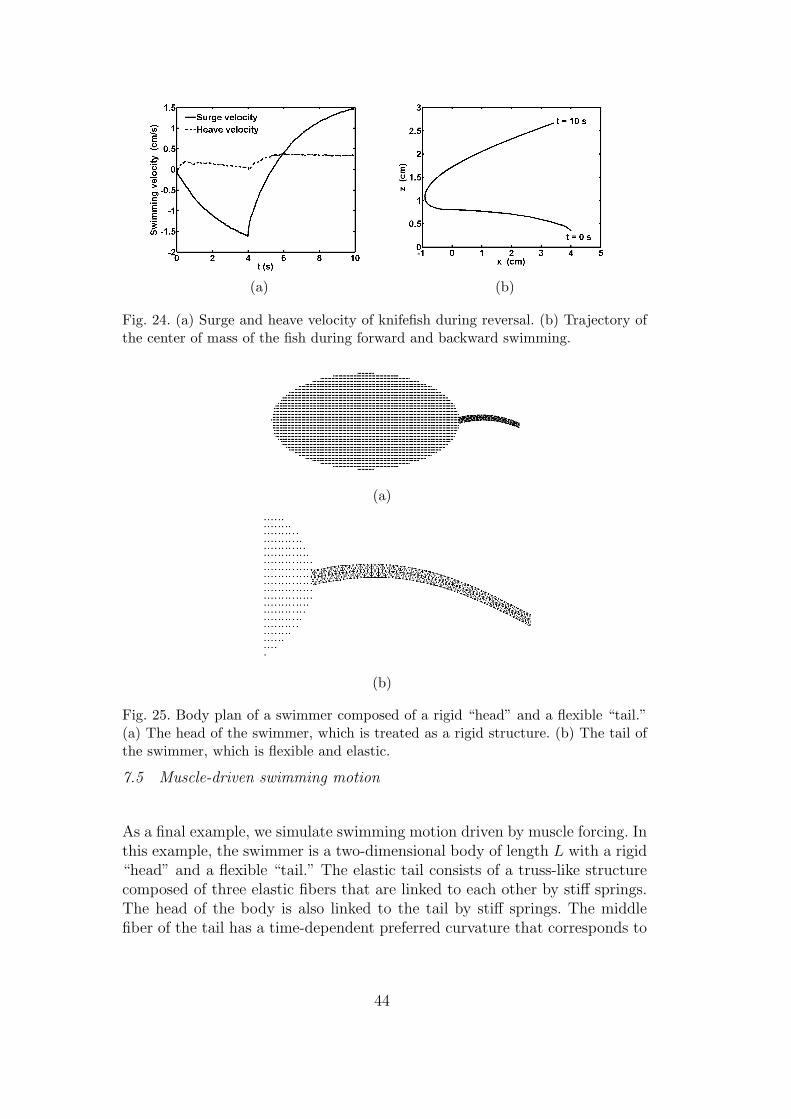
(a) (b)

Fig. 24. (a) Surge and heave velocity of knifefish during reversal. (b) Trajectory ofthe center of mass of the fish during forward and backward swimming.

(a)

(b)

Fig. 25. Body plan of a swimmer composed of a rigid “head” and a flexible “tail.”(a) The head of the swimmer, which is treated as a rigid structure. (b) The tail ofthe swimmer, which is flexible and elastic.

7.5 Muscle-driven swimming motion

As a final example, we simulate swimming motion driven by muscle forcing. Inthis example, the swimmer is a two-dimensional body of length L with a rigid“head” and a flexible “tail.” The elastic tail consists of a truss-like structurecomposed of three elastic fibers that are linked to each other by stiff springs.The head of the body is also linked to the tail by stiff springs. The middlefiber of the tail has a time-dependent preferred curvature that corresponds to

44

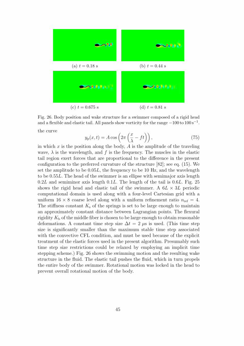
(a) t = 0.18 s (b) t = 0.44 s

(c) t = 0.675 s (d) t = 0.81 s

Fig. 26. Body position and wake structure for a swimmer composed of a rigid headand a flexible and elastic tail. All panels show vorticity for the range −100 to 100 s−1.

the curve

yp(x, t) = A cos(2π(

x

λ− ft

)), (75)

in which x is the position along the body, A is the amplitude of the travelingwave, λ is the wavelength, and f is the frequency. The muscles in the elastictail region exert forces that are proportional to the difference in the presentconfiguration to the preferred curvature of the structure [82]; see eq. (15). Weset the amplitude to be 0.05L, the frequency to be 10 Hz, and the wavelengthto be 0.55L. The head of the swimmer is an ellipse with semimajor axis length0.2L and semiminor axis length 0.1L. The length of the tail is 0.6L. Fig. 25shows the rigid head and elastic tail of the swimmer. A 6L × 3L periodiccomputational domain is used along with a four-level Cartesian grid with auniform 16 × 8 coarse level along with a uniform refinement ratio nref = 4.The stiffness constant Ks of the springs is set to be large enough to maintainan approximately constant distance between Lagrangian points. The flexuralrigidity Kb of the middle fiber is chosen to be large enough to obtain reasonabledeformations. A constant time step size ∆t = 2 µs is used. (This time stepsize is significantly smaller than the maximum stable time step associatedwith the convective CFL condition, and must be used because of the explicittreatment of the elastic forces used in the present algorithm. Presumably suchtime step size restrictions could be relaxed by employing an implicit timestepping scheme.) Fig. 26 shows the swimming motion and the resulting wakestructure in the fluid. The elastic tail pushes the fluid, which in turn propelsthe entire body of the swimmer. Rotational motion was locked in the head toprevent overall rotational motion of the body.

45

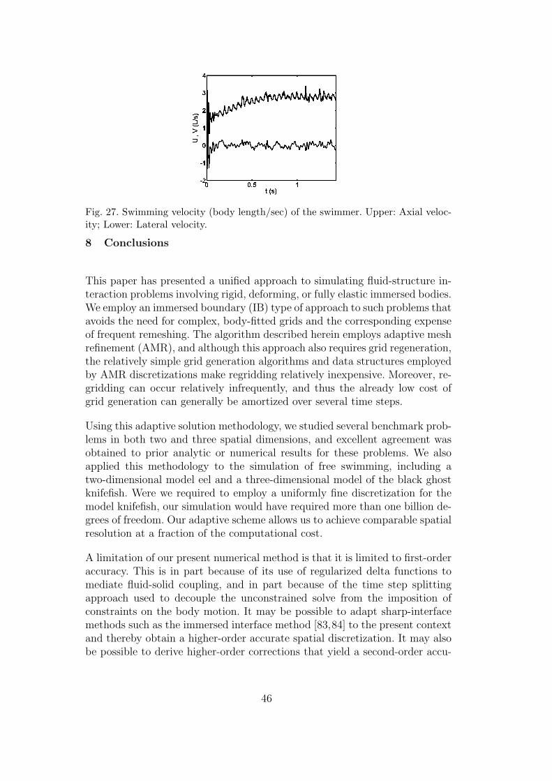
Fig. 27. Swimming velocity (body length/sec) of the swimmer. Upper: Axial veloc-ity; Lower: Lateral velocity.

8 Conclusions

This paper has presented a unified approach to simulating fluid-structure in-teraction problems involving rigid, deforming, or fully elastic immersed bodies.We employ an immersed boundary (IB) type of approach to such problems thatavoids the need for complex, body-fitted grids and the corresponding expenseof frequent remeshing. The algorithm described herein employs adaptive meshrefinement (AMR), and although this approach also requires grid regeneration,the relatively simple grid generation algorithms and data structures employedby AMR discretizations make regridding relatively inexpensive. Moreover, re-gridding can occur relatively infrequently, and thus the already low cost ofgrid generation can generally be amortized over several time steps.

Using this adaptive solution methodology, we studied several benchmark prob-lems in both two and three spatial dimensions, and excellent agreement wasobtained to prior analytic or numerical results for these problems. We alsoapplied this methodology to the simulation of free swimming, including atwo-dimensional model eel and a three-dimensional model of the black ghostknifefish. Were we required to employ a uniformly fine discretization for themodel knifefish, our simulation would have required more than one billion de-grees of freedom. Our adaptive scheme allows us to achieve comparable spatialresolution at a fraction of the computational cost.

A limitation of our present numerical method is that it is limited to first-orderaccuracy. This is in part because of its use of regularized delta functions tomediate fluid-solid coupling, and in part because of the time step splittingapproach used to decouple the unconstrained solve from the imposition ofconstraints on the body motion. It may be possible to adapt sharp-interfacemethods such as the immersed interface method [83,84] to the present contextand thereby obtain a higher-order accurate spatial discretization. It may alsobe possible to derive higher-order corrections that yield a second-order accu-

46

rate method, similar to the approach used by Brown, Cortez, and Minion [85]to develop fully second-order accurate versions of the projection method forincompressible flow. Alternatively, achieving full second-order accuracy mayrequire the development of an unsplit solver. The construction of an efficienthigher-order accurate version of the present scheme remains challenging futurework.

A final remark about our implementation is that it is presently restrictedto constant-coefficient fluid solves, although we emphasize that this is nota limitation of the present mathematical formulation. This limitation makesit challenging to simulate immersed bodies that are not neutrally buoyant.Approaches similar to the penalty IB method [86] could possibly be used toaccount for bodies with mass densities greater than that of the fluid. An alter-native is to employ a variable-density fluid solver, which makes it straightfor-ward to model immersed bodies that are either more dense or less dense thanthe surrounding fluid [35–38]. Likewise, robust variable-coefficient fluid solverscould enable efficient simulations of truly elastic bodies by removing the vis-cous stresses from the elastic parts of the structure. Such extensions, whichwe and others are actively pursuing, will further strengthen this approach tosimulating fluid-structure interaction.

Acknowledgements

A.P.S.B. acknowledges helpful discussions with Anup A. Shirgaonkar, OscarM. Curet, and Srinivas Ramakrishnan over the course of this work. A.P.S.B,R.B, and N.A.P acknowledge computational resources provided by North-western University’s Quest high performance computing service and MalcolmA. MacIver for providing experimental kinematic data of the black ghostknifefish. We thank Aleksandar Donev for his suggestions on improving themanuscript. B.E.G. acknowledges research support from the National ScienceFoundation (NSF awards DMS-1016554 and OCI-1047734). A.P.S.B., R.B.,and N.A.P. acknowledge research support from the National Science Founda-tion (NSF awards CBET-0828749, CBET-1066575, and CMMI-0941674).

References

[1] H. H. Hu, N. A. Patankar, M. Y. Zhu, Direct numerical simulations offluid-solid systems using the arbitrary Lagrangian-Eulerian technique, JComput Phys 169 (2001) 427–462.

[2] S. Kern, P. Koumoutsakos, Simulations of optimized anguilliform swimming, JExpt Biol 209 (2006) 4841–4857.

47

[3] C. S. Peskin, The immersed boundary method, Acta Numer 11 (2002)479–517.

[4] M.-C. Lai, Z.-L. Li, A remark on jump conditions for the three-dimensionalNavier-Stokes equations involving an immersed moving membrane, Appl MathLett 14 (2) (2001) 149–154.

[5] S. Xu, Z. J. Wang, Systematic derivation of jump conditions for the immersedinterface method in three-dimensional flow simulation, SIAM J Sci Comput27 (6) (2006) 1948–1980.

[6] A. M. Roma, C. S. Peskin, M. J. Berger, An adaptive version of the immersedboundary method, J Comput Phys 153 (2) (1999) 509–534.

[7] B. E. Griffith, R. D. Hornung, D. M. McQueen, C. S. Peskin, An adaptive,formally second order accurate version of the immersed boundary method,J Comput Phys 223 (1) (2007) 10–49.

[8] B. E. Griffith, R. D. Hornung, D. M. McQueen, C. S. Peskin, Parallel andadaptive simulation of cardiac fluid dynamics, in: M. Parashar, X. Li (Eds.),Advanced Computational Infrastructures for Parallel and DistributedAdaptive Applications, John Wiley and Sons, Hoboken, NJ, USA, 2009.

[9] B. E. Griffith, Immersed boundary model of aortic heart valve dynamics withphysiological driving and loading conditions, Int J Numer Meth Biomed Eng28 (3) (2012) 317–345.

[10] R. Glowinski, T.-W. Pan, T. I. Hesla, D. D. Joseph, A distributed Lagrangemultiplier/fictitious domain method for particulate flows, Int J MultiphasFlow 25 (1999) 755–794.

[11] N. A. Patankar, P. Singh, D. D. Joseph, R. Glowinski, T. Pan, A newformulation of the distributed Lagrange multiplier/fictitious domain methodfor particulate flows, Int J Multiphas Flow 26 (2000) 1509–1524.

[12] N. A. Patankar, A formulation for fast computations of rigid particulate flows,Tech. rep., Center for Turbulence Research Annual Research Briefs,http://ctr.stanford.edu (2001).

[13] N. A. Patankar, Physical interpretation and mathematical properties of thestress-DLM formulation for rigid particulate flows, Int J Comput Method EngSci Mech 6 (2005) 137–143.

[14] A. A. Shirgaonkar, M. A. MacIver, N. A. Patankar, A new mathematicalformulational and fast algorithm for fully resolved simulation ofself-propulsion, J Comput Phys 228 (2009) 2366–2390.

[15] A. J. Chorin, Numerical solution of the Navier-Stokes equations, MathComput 22 (104) (1968) 745–762.

[16] M. J. Berger, J. Oliger, Adaptive mesh refinement for hyperbolicpartial-differential equations, J Comput Phys 53 (3) (1984) 484–512.

48

[17] M. J. Berger, P. Colella, Local adaptive mesh refinement for shockhydrodynamics, J Comput Phys 82 (1) (1989) 64–84.

[18] L. J. Fauci, C. S. Peskin, A computational model of aquatic animallocomotion, J Comput Phys 77 (1988) 85–108.

[19] E. D. Tytell, C.-Y. Hsu, T. L. Williams, A. H. Cohen, L. J. Fauci, Interactionsbetween internal forces, body stiffness, and fluid environment in aneuromechanical model of lamprey swimming, Proc Natl Acad Sci U S A 107(2010) 19832–19837.

[20] H. Zhao, J. B. Freund, R. D. Moser, A fixed-mesh method for incompressibleflow-structure systems with finite solid deformations, J Comput Phys 227(2008) 3114–3140.

[21] G. Herschlag, L. Miller, Reynolds number limits for jet propulsion: Anumerical study of simplified jellyfish, J Theor Biol 285 (2011) 84–95.

[22] R. Mittal, Computational modeling in bio-hydrodynamics: trends, challengesand recent advances, IEEE J Ocean Eng 29 (2004) 595–604.

[23] R. Mittal, H. Dong, G. V. Lauder, Locomotion with flexible propulsors. II:Computational modeling of pectoral fin swimming in sunfish, Bioinsp Biomim1 (2006) S35–S41.

[24] I. Borazjani, F. Sotiropoulos, Numerical investigation of the hydrodynamics ofcrangiform swimming in the translational and inertial flow regimes, J ExptBiol 211 (2008) 1541–1558.

[25] A. A. Shirgaonkar, O. M. Curet, N. A. Patankar, M. A. MacIver, Thehydrodynamics of ribbon-fin propulsion during impulsive motion, J Expt Biol211 (2008) 3490–3503.

[26] O. M. Curet, I. K. AlAli, M. A. MacIver, N. A. Patankar, A versatile implicititerative approach for fully resolved simulations of self-propulsion, ComputMeth Appl Mech Eng 199 (2010) 2336–2390.

[27] M. Bergmann, A. Iollo, Modeling and simulation of fish-like swimming, JComput Phys 230 (2011) 329–348.

[28] G. V. Lauder, Function of the caudal fin during locomotion in fishes:kinematics, flow visualization, and evolutionary patterns, Am Zool 40 (2000)101–122.

[29] G. V. Lauder, J. C. Nauen, E. G. Drucker, Experimental hydrodynamics andevolution: function of median fins in ray-finned fishes, Integr Comp Biol 42(2002) 1009–1017.

[30] J. O. Dabiri, M. Gharib, Sensitivity analysis of kinematic approximations indynamic medusan swimming models, J Expt Biol 206 (2003) 3675–3680.

[31] E. D. Tytell, G. V. Lauder, The hydrodynamics of eel swimming. I: Wakestructure, J Expt Biol 207 (2004) 1825–1841.

49

[32] O. M. Curet, N. A. Patankar, G. V. Lauder, M. A. MacIver, Aquaticmanoeuvering with counter-propagating waves: a novel locomotive strategy, JR Soc Interface 8 (2011) 1041–1050.

[33] O. M. Curet, N. A. Patankar, G. V. Lauder, M. A. MacIver, Mechanicalproperties of a bio-inspired robotic knifefish with an undulatory propulsor,Bioinspir Biomim 6 (2011) 026004.

[34] R. Ruiz-Torres, O. M. Curet, G. V. Lauder, M. A. MacIver, Kinematics of theribbon fin in hovering and swimming of the electric ghost knifefish, J ExptBiol (in press).

[35] S. V. Apte, M. Martin, N. A. Patankar, A numerical method for fully resolvedsimulation (FRS) of rigid particle-flow interactions in complex flows, JComput Phys 228 (2009) 2712–2738.

[36] S. Apte, J. Finn, A Variable-Density Fictitious-Domain Method for FullyResolved Simulation of High-Density Ratio Fluid-Particle Systems, in: 7thInternational Conference on Multiphas Flow, 2010, 13 pages.

[37] T. G. Fai, B. E. Griffith, Y. Mori, C. S. Peskin, Immersed boundary methodfor variable viscosity and variable density problems using fast linear solvers. I:Numerical method and results, Manuscript submitted for publication.

[38] T. G. Fai, B. E. Griffith, Y. Mori, C. S. Peskin, Immersed boundary methodfor variable viscosity and variable density problems using fast linear solvers.II: Theory, Manuscript submitted for publication.

[39] B. E. Griffith, X. Luo, D. M. McQueen, C. S. Peskin, Simulating the fluiddynamics of natural and prosthetic heart valves using the immersed boundarymethod, Int J Appl Mech 1 (1) (2009) 137–177.

[40] L. Zhang, A. Gerstenberger, X. Wang, W. K. Liu, Immersed finite elementmethod, Comput Meth Appl Mech Eng 193 (21–22) (2004) 2051–2067.

[41] W. K. Liu, Y. Liu, D. Farrell, L. Zhang, X. S. Wang, Y. Fukui, N. Patankar,Y. Zhang, C. Bajaj, J. Lee, J. Hong, X. Chen, H. Hsu, Immersed finiteelement method and its applications to biological systems, Comput MethAppl Mech Eng 195 (13–16) (2006) 1722–1749.

[42] D. Boffi, L. Gastaldi, L. Heltai, C. S. Peskin, On the hyper-elastic formulationof the immersed boundary method, Comput Meth Appl Mech Engrg197 (25–28) (2008) 2210–2231.

[43] D. Devendran, C. S. Peksin, An energy-based immersed boundary method forincompressible viscoelasticity, J Comput Phys 231 (14) (2012) 4613–4642.

[44] B. E. Griffith, X. Luo, Hybrid finite difference/finite element version of theimmersed boundary method (submitted, preprint available fromhttp://www.cims.nyu.edu/ griffith).

[45] B. E. Griffith, C. S. Peskin, On the order of accuracy of the immersedboundary method: Higher order convergence rates for sufficiently smoothproblems, J Comput Phys 208 (1) (2005) 75–105.

50

[46] W. J. Rider, J. A. Greenough, J. R. Kamm, Accurate monotonicity- andextrema-preserving methods through adaptive nonlinear hybridizations,J Comput Phys 225 (2) (2007) 1827–1848.

[47] P. Colella, P. R. Woodward, The piecewise parabolic method (PPM) forgas-dynamical simulations, J Comput Phys 54 (1) (1984) 174–201.

[48] Y. Saad, A flexible inner-outer preconditioned GMRES algorithm,SIAM J Sci Comput 14 (2) (1993) 461–469.

[49] B. E. Griffith, An accurate and efficient method for the incompressibleNavier-Stokes equations using the projection method as a preconditioner, JComput Phys 228 (20) (2009) 7565–7595.

[50] M. J. Berger, I. Rigoutsos, An algorithm for point clustering and gridgeneration, IEEE Trans Syst Man Cybern 21 (5) (1991) 1278–1286.

[51] G. Toth, P. L. Roe, Divergence- and curl-preserving prolongation andrestriction formulas, J Comput Phys 180 (2) (2002) 736–750.

[52] IBAMR: An adaptive and distributed-memory parallel implementation of theimmersed boundary method, http://ibamr.googlecode.com.

[53] SAMRAI: Structured Adaptive Mesh Refinement Application Infrastructure,http://www.llnl.gov/CASC/SAMRAI.

[54] R. D. Hornung, S. R. Kohn, Managing application complexity in the SAMRAIobject-oriented framework, Concurrency Comput Pract Ex 14 (5) (2002)347–368.

[55] R. D. Hornung, A. M. Wissink, S. R. Kohn, Managing complex data andgeometry in parallel structured AMR applications, Eng Comput 22 (3–4)(2006) 181–195.

[56] S. Balay, K. Buschelman, W. D. Gropp, D. Kaushik, M. G. Knepley, L. C.McInnes, B. F. Smith, H. Zhang, PETSc Web page,http://www.mcs.anl.gov/petsc (2009).

[57] S. Balay, K. Buschelman, V. Eijkhout, W. D. Gropp, D. Kaushik, M. G.Knepley, L. C. McInnes, B. F. Smith, H. Zhang, PETSc users manual, Tech.Rep. ANL-95/11 - Revision 3.0.0, Argonne National Laboratory (2008).

[58] S. Balay, V. Eijkhout, W. D. Gropp, L. C. McInnes, B. F. Smith, Efficientmanagement of parallelism in object oriented numerical software libraries, in:E. Arge, A. M. Bruaset, H. P. Langtangen (Eds.), Modern Software Tools inScientific Computing, Birkhauser Press, 1997, pp. 163–202.

[59] hypre: High performance preconditioners,http://www.llnl.gov/CASC/hypre.

[60] R. D. Falgout, U. M. Yang, hypre: a library of high performancepreconditioners, in: P. M. A. Sloot, C. J. K. Tan, J. J. Dongarra, A. G.Hoekstra (Eds.), Computational Science - ICCS 2002 Part III, Vol. 2331 of

51

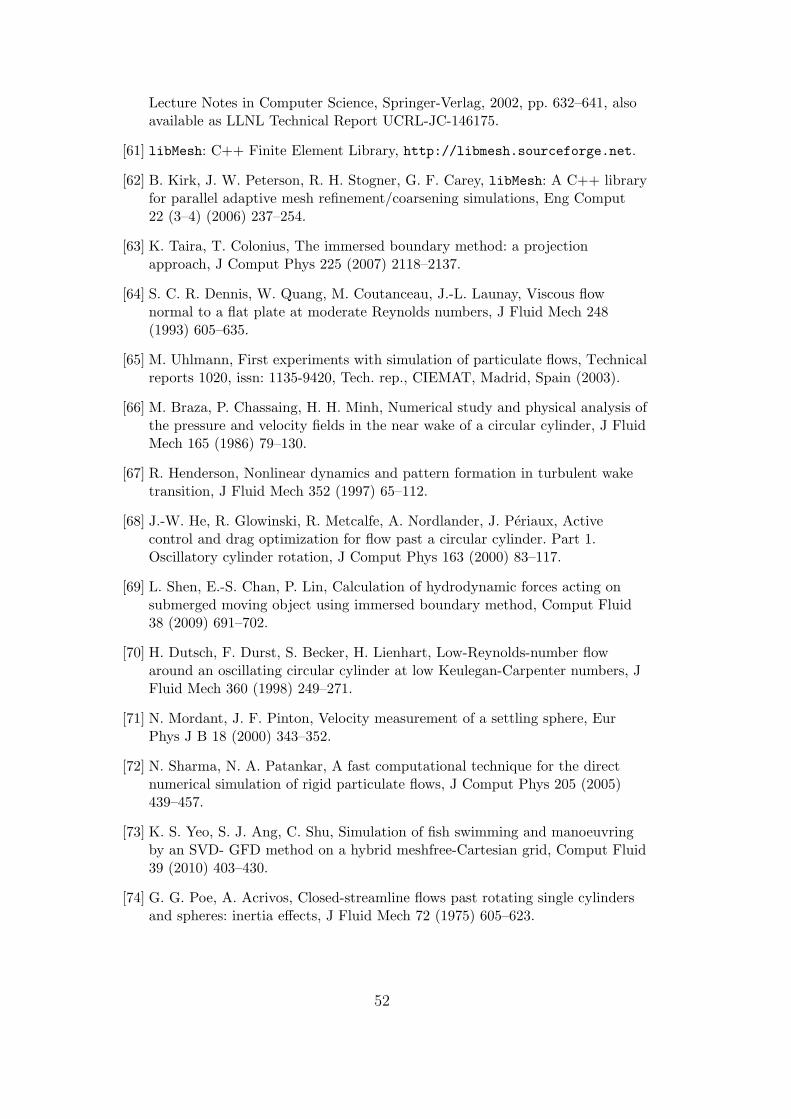
Lecture Notes in Computer Science, Springer-Verlag, 2002, pp. 632–641, alsoavailable as LLNL Technical Report UCRL-JC-146175.

[61] libMesh: C++ Finite Element Library, http://libmesh.sourceforge.net.

[62] B. Kirk, J. W. Peterson, R. H. Stogner, G. F. Carey, libMesh: A C++ libraryfor parallel adaptive mesh refinement/coarsening simulations, Eng Comput22 (3–4) (2006) 237–254.

[63] K. Taira, T. Colonius, The immersed boundary method: a projectionapproach, J Comput Phys 225 (2007) 2118–2137.

[64] S. C. R. Dennis, W. Quang, M. Coutanceau, J.-L. Launay, Viscous flownormal to a flat plate at moderate Reynolds numbers, J Fluid Mech 248(1993) 605–635.

[65] M. Uhlmann, First experiments with simulation of particulate flows, Technicalreports 1020, issn: 1135-9420, Tech. rep., CIEMAT, Madrid, Spain (2003).

[66] M. Braza, P. Chassaing, H. H. Minh, Numerical study and physical analysis ofthe pressure and velocity fields in the near wake of a circular cylinder, J FluidMech 165 (1986) 79–130.

[67] R. Henderson, Nonlinear dynamics and pattern formation in turbulent waketransition, J Fluid Mech 352 (1997) 65–112.

[68] J.-W. He, R. Glowinski, R. Metcalfe, A. Nordlander, J. Periaux, Activecontrol and drag optimization for flow past a circular cylinder. Part 1.Oscillatory cylinder rotation, J Comput Phys 163 (2000) 83–117.

[69] L. Shen, E.-S. Chan, P. Lin, Calculation of hydrodynamic forces acting onsubmerged moving object using immersed boundary method, Comput Fluid38 (2009) 691–702.

[70] H. Dutsch, F. Durst, S. Becker, H. Lienhart, Low-Reynolds-number flowaround an oscillating circular cylinder at low Keulegan-Carpenter numbers, JFluid Mech 360 (1998) 249–271.

[71] N. Mordant, J. F. Pinton, Velocity measurement of a settling sphere, EurPhys J B 18 (2000) 343–352.

[72] N. Sharma, N. A. Patankar, A fast computational technique for the directnumerical simulation of rigid particulate flows, J Comput Phys 205 (2005)439–457.

[73] K. S. Yeo, S. J. Ang, C. Shu, Simulation of fish swimming and manoeuvringby an SVD- GFD method on a hybrid meshfree-Cartesian grid, Comput Fluid39 (2010) 403–430.

[74] G. G. Poe, A. Acrivos, Closed-streamline flows past rotating single cylindersand spheres: inertia effects, J Fluid Mech 72 (1975) 605–623.

52

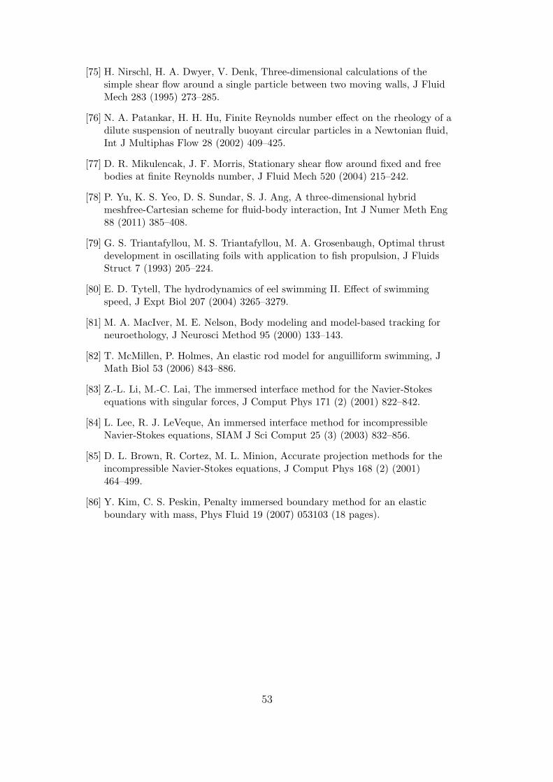
[75] H. Nirschl, H. A. Dwyer, V. Denk, Three-dimensional calculations of thesimple shear flow around a single particle between two moving walls, J FluidMech 283 (1995) 273–285.

[76] N. A. Patankar, H. H. Hu, Finite Reynolds number effect on the rheology of adilute suspension of neutrally buoyant circular particles in a Newtonian fluid,Int J Multiphas Flow 28 (2002) 409–425.

[77] D. R. Mikulencak, J. F. Morris, Stationary shear flow around fixed and freebodies at finite Reynolds number, J Fluid Mech 520 (2004) 215–242.

[78] P. Yu, K. S. Yeo, D. S. Sundar, S. J. Ang, A three-dimensional hybridmeshfree-Cartesian scheme for fluid-body interaction, Int J Numer Meth Eng88 (2011) 385–408.

[79] G. S. Triantafyllou, M. S. Triantafyllou, M. A. Grosenbaugh, Optimal thrustdevelopment in oscillating foils with application to fish propulsion, J FluidsStruct 7 (1993) 205–224.

[80] E. D. Tytell, The hydrodynamics of eel swimming II. Effect of swimmingspeed, J Expt Biol 207 (2004) 3265–3279.

[81] M. A. MacIver, M. E. Nelson, Body modeling and model-based tracking forneuroethology, J Neurosci Method 95 (2000) 133–143.

[82] T. McMillen, P. Holmes, An elastic rod model for anguilliform swimming, JMath Biol 53 (2006) 843–886.

[83] Z.-L. Li, M.-C. Lai, The immersed interface method for the Navier-Stokesequations with singular forces, J Comput Phys 171 (2) (2001) 822–842.

[84] L. Lee, R. J. LeVeque, An immersed interface method for incompressibleNavier-Stokes equations, SIAM J Sci Comput 25 (3) (2003) 832–856.

[85] D. L. Brown, R. Cortez, M. L. Minion, Accurate projection methods for theincompressible Navier-Stokes equations, J Comput Phys 168 (2) (2001)464–499.

[86] Y. Kim, C. S. Peskin, Penalty immersed boundary method for an elasticboundary with mass, Phys Fluid 19 (2007) 053103 (18 pages).

53

A unified mathematical framework and an adaptive numerical method for fluid–structure interaction...

Documents

Transcript of A unified mathematical framework and an adaptive numerical method for fluid–structure interaction...