International Journal of Non-Linear Mechanics 47 (2012) 626–638

Contents lists available at SciVerse ScienceDirect

International Journal of Non-Linear Mechanics

0020-74

doi:10.1

n Corr

E-m

journal homepage: www.elsevier.com/locate/nlm

A modified SPH method for simulating motion of rigid bodies in Newtonianfluid flows

M.R. Hashemi a, R. Fatehi b, M.T. Manzari a,n

a Center of Excellence in Energy Conversion, School of Mechanical Engineering, Sharif University of Technology, Tehran, Iranb Department of Mechanical Engineering, Persian Gulf University, Boushehr 75168, Iran

a r t i c l e i n f o

Article history:

Received 25 October 2010

Received in revised form

19 October 2011

Accepted 20 October 2011Available online 29 October 2011

Keywords:

Smoothed particle hydrodynamics (SPH)

Weakly compressible

Particulate flow

Boundary condition

Consistency

62/$ - see front matter & 2011 Elsevier Ltd. A

016/j.ijnonlinmec.2011.10.007

esponding author. Tel.: þ98 21 6616 5689; f

ail address: mtmanzari@sharif.edu (M.T. Man

a b s t r a c t

A weakly compressible smoothed particle hydrodynamics (WCSPH) method is used along with a new

no-slip boundary condition to simulate movement of rigid bodies in incompressible Newtonian fluid

flows. It is shown that the new boundary treatment method helps to efficiently calculate the

hydrodynamic interaction forces acting on moving bodies. To compensate the effect of truncated

compact support near solid boundaries, the method needs specific consistent renormalized schemes for

the first and second-order spatial derivatives. In order to resolve the problem of spurious pressure

oscillations in the WCSPH method, a modification to the continuity equation is used which improves

the stability of the numerical method. The performance of the proposed method is assessed by solving a

number of two-dimensional low-Reynolds fluid flow problems containing circular solid bodies.

Wherever possible, the results are compared with the available numerical data.

& 2011 Elsevier Ltd. All rights reserved.

1. Introduction

Particulate flows represent a particular type of fluid–solidinteraction problems which have a wide range of applications inindustry from biological suspensions to liquid–solid mixtures inmining industry. The rheological characteristics of such flows areof prime interest to engineers. These macroscopic characteristicscan be described by various hydrodynamic interactions betweensolid(s) and the surrounding fluid. To investigate such interac-tions, one needs to accurately determine the hydrodynamic forcesexchanged between the fluid and solid particles. This can beachieved using computational techniques which can properlyhandle moving boundaries and fluid–solid interfaces. One approachwhich is widely adopted in this context is to use a Lagrangianframework along with mesh-free methods.

Unlike Eulerian approach which uses a fixed frame of referenceto analyze what happens at every fixed point in space, theLagrangian viewpoint follows the trajectory of individual lumps ofmaterial. This viewpoint is particularly useful for flow problems asin the Lagrangian formulations, convective terms vanish and thecomplexity of numerical method due to the presence of these termsis alleviated. Besides when the problem involves movement of solidparts, the interface between solid and fluid does not cross thecomputational grid, hence facilitating treatment of such interfaces.

ll rights reserved.

ax: þ98 21 6600 0021.

zari).

A particularly useful type of computational methods are themesh-free (particle-based) methods. These can be used alongwith both Eulerian and Lagrangian approaches and can add moreflexibility to the underlying method. In these methods, computa-tional particles represent the actual fluid and solid domains.These particles can move inside the computational domaintransporting physical quantities such as mass, momentum andenergy. The mesh-free methods do not face problems such asmesh entanglement and interface dispersion.

One of the most popular particle-based Lagrangian methods isthe smoothed particle hydrodynamics (SPH) method introduced byLucy [1] and Gingold and Monaghan [2] in 1977. The accuracy andstability of the SPH method has been constantly improved and it hasbeen successfully used in many engineering problems [3–5]. Twodifferent approaches are usually adopted in SPH for solving incom-pressible fluid flow problems: (1) using a weakly compressible fluidconcept [6,5] and (2) using a projection method [7–10].

This paper attempts to solve particulate flows using the WCSPHmethod. To do this, the SPH method needs further improvements inthree areas: (1) devising a generalized methodology for impositionof various boundary conditions on the solid boundaries, (2) usingconsistent formulations for spatial differentiations, and (3) decreas-ing spurious pressure oscillations.

The first area of improvement is the imposition of solid boundarycondition. This is of prime importance to a particulate flow as theforces exchanged between the solid and fluid are determined viathis mechanism. There are three major solid boundary treatmenttechniques in the SPH method.

M.R. Hashemi et al. / International Journal of Non-Linear Mechanics 47 (2012) 626–638 627

One approach used dummy SPH particles which are the sameas fluid SPH particles and are attached in the form of some layersof particles to the solid body [5,8]. Potapov and his co-workerssolved a particulate flow problem using this approach for solidboundaries [11].

The second approach for imposition of solid boundary condi-tion is to use the so-called mirror SPH particles. These particleshave the same properties as the fluid SPH particles and provide amirror effect on the other side of the solid boundary [7,12]. As aresult, when a fluid particle approaches the solid boundary andattempts to leave the domain, a mirror particle does the same andattempts to enter the domain, hence imposing enough force toprevent the fluid particle from penetrating the boundary. Theimpact of a wedge to the water surface was simulated by Ogeret al. using this type of solid boundary [13]. Shao [14] reportedthat although this approach produces acceptable results but it canbe computationally expensive. Also, this approach may encounterdifficulty for geometrically complex solid surfaces [15].

The third approach is to use a set of boundary particles whichexert repulsive forces to the neighboring fluid SPH particles. Therepulsive force is obtained from either the Lennard-Jones force[16] or gradient of the kernel function [17,18]. To obtain satisfac-tory results, the repulsive force function must be chosen carefully[15,17]. Unfortunately, the choice of this function is not obvious.

In this paper, a new solid boundary treatment is introducedwhich supersedes the above-mentioned methods for particulateflow problems.

The second area of improvement is related to the use ofconsistent spatial derivative schemes in the SPH method. Manyof such schemes are not consistent and this ultimately affects theglobal accuracy of the method. In this paper, consistent schemesto be used along with the weakly compressible SPH method areemployed. The so-called renormalized schemes are used for thefirst-order and second-order spatial derivatives [4,19].

Numerical experiences have shown that when the WCSPHmethod is used, spurious oscillations can occur in the pressure field[10] as a result of some kind of decoupling between primitivevariables originated from the use of improper combination of spatialderivatives [20]. To improve this aspect of the SPH method, amodified continuity equation is used in this paper.

In the following, first the governing equations are presentedfollowed by a brief description of the weakly compressible SPHmethod. This is followed by presenting the new fluid–solid boundarytreatment. Next, the equation of motion of the solid bodies ispresented. Then, the time integration procedure is described. Finally,a number of two-dimensional test cases involving particle migrationin shear flows and falling of particle(s) in a closed channel are studied.

2. Basic equations

In this work, laminar incompressible Newtonian fluid flows areconsidered for which the mass and momentum conservationequations are

drdt¼�rr � V, ð1Þ

rdV

dt¼�rPþmr2Vþrg, ð2Þ

where r is the density of the fluid, P is the pressure and V is thevelocity vector. Also, g represents the gravity acceleration and m isthe dynamic viscosity of the fluid. To close this system of equations,an equation of state is required to describe the variation of densitywith pressure. A simple and frequently used equation of state is

P�P0 ¼ c2ðr�r0Þ ð3Þ

in which c¼ffiffiffiffiffiffiffiffiffiffiffiffiffiffiffiffiffiffið@P=@rÞs

pis the speed of sound defined for an

isentropic process. In this work, the fluid is considered incompres-sible and therefore the above equation of state is accurate enough.Eqs. (1) and (2) are solved using the SPH method. In the following,the solution procedure is described briefly.

3. SPH formulation

The SPH method is built on the notion of interpolation and theSPH particles hold the required variables for this interpolation.Here, each particle has a circular compact support of radius h. Foran arbitrary field function u, the interpolated value /uS atposition r is computed from

/uðrÞS¼X

j

ojujWð9r�rj9,hÞ, ð4Þ

where oj is the volume of neighboring particle j and W is a positivesmoothing or kernel function representing Dirac delta function [2].A successful numerical method for solving Eqs. (1) and (2), requiresfairly accurate discretizations of the spatial derivatives of the fieldvariables. In the following, techniques used for spatial derivativesare briefly described.

3.1. Spatial derivatives

There are various schemes for the discretization of the spatialderivatives in SPH. To have a convergent numerical method, thediscretization schemes used in the method must be consistent.This means that truncation error of each scheme must approachzero as the particle spacing d decreases. In practice, however,most of available schemes in SPH, do not have this importantproperty. Indeed, in general, the truncation error vanishes onlywhen d goes to zero much faster than the smoothing radius h ofthe kernel function [21], that is h=d�!1. The ratio h=d controlsthe number of neighboring particles. Note that this ratio directlycorrelates with the number of computations and a large value canlead to a prohibitive computational cost.

For discretization of the first derivatives in SPH, Randles andLibersky [4] introduced a first-order consistent scheme. The first-order consistency property means that the scheme predicts the firstderivative of linear functions exactly [22]. The numerical approx-imation of the first derivative /ruSi can be obtained as [4]

/ruSi ¼X

j

ojBi � rWijðuj�uiÞ, ð5Þ

where Wij ¼Wð9rij9,hÞ is the value of smoothing or kernel functionof particle i at the position of particle j and rij ¼ ri�rj. Also,

Bi ¼�X

j

ojrijrWij

24

35�1

ð6Þ

is a renormalization tensor [23,24]. Since rWij is parallel to rij, therenormalization tensor B is symmetric. Using Taylor series expan-sion about ri, it can be shown that the truncation error of the abovescheme is [19]

/ruSi�ru9i ¼1

2rru9i :

Xj

ojBi � rWijrijrijþ � � � , ð7Þ

where the operator ‘‘:’’ denotes the inner product of second-ordertensors. Note that the leading term in the truncation error includesthe second derivativerru9i, therefore, the method is consistent andconverges linearly as d�!0 for a constant ratio h=d.

The computation of second-order spatial derivative plays animportant role in the flow Equation. (2). Among all second derivativeapproximation schemes, Basa et al. [25] showed that a fairly accurate

M.R. Hashemi et al. / International Journal of Non-Linear Mechanics 47 (2012) 626–638628

formula is

/r2uSi ¼X

j

2oj

ui�uj

rijeij � rWij, ð8Þ

where rij ¼ 9rij9 and eij ¼ rij=rij is a unit vector in the inter-particledirection. The truncation error of (8) is [19]

/r2uSi�ru29i ¼ 2ru9i �X

j

ojrWijþrru9i : ðB�1i �IÞ

þ1

3rrru9i^

Xj

ojrijrijrWij

0@

1Aþ � � � : ð9Þ

A suitable method for discretization of second derivatives shouldinclude at least third-order derivativerrru9i as the leading term ofits truncation error. The truncation error in Eq. (9) has two extraterms. To improve the accuracy of this scheme, the effect of theseterms should be decreased. An alternative scheme was recentlyintroduced by Fatehi and Manzari [19] as

/r2uSi ¼ B̂ i :X

j

2ojeijrWij

ui�uj

rij�/eij � ruSi

� �, ð10Þ

where /ruSi is computed according to Eq. (5) and B̂ is a newrenormalization tensor which is computed using the following set ofequations:

B̂i :X

j

ojrijeijeijrWijþX

j

ojeijeijrWij

0@

1A

24 �Bi �

Xj

ojrijrijrWij

0@

1A35¼�I:

ð11Þ

Here I is the second-order identity tensor. Using this secondderivative scheme, smaller number of neighboring particles(or equivalently smaller kernel cutoff distance) than usualschemes, is needed to give an acceptable accuracy. For instance,in a two-dimensional incompressible flow, about 50 neighbors areneeded for each particle to approximate the second derivative ofthe velocity field for computation of viscous terms in the Navier–Stokes equation using a typical SPH scheme. However, in this work,this number is as low as about 20. This leads to less computationalcost and ultimately a faster algorithm, though calculation of therenormalization tensors requires some extra computational effortsin the proposed method.

It must be noted that, the renormalization tensors, B̂ and B,reduce the error caused by the truncated SPH particles distribu-tion near solid boundaries. For the SPH particles whose neighborsare all inside the flow domain, B̂ and B become approximatelyidentity tensors. For SPH particles in the neighborhood of a solidboundary, where there is a deficiency in SPH particles distribu-tion, the entities of these tensors increase significantly to properlycompensate the lack of the neighboring SPH particles. Thisproperty improves the evaluation of boundary particles contribu-tion and facilitates the implementation of a new no-slip boundarycondition. This will be elaborated in Section 4.

The governing equations to be solved can be summarized as

d

dt

V

r

( )¼�rP

r þnr2Vþg

�rr � V

( ), ð12Þ

where n¼ m=r is the kinematic viscosity. Solving the set ofequations (12) may lead to solutions with non-physical oscilla-tions in pressure especially for the complex flows with significantchanges in the pressure. To avoid this problem, a modification tothe mass conservation equation should be made. This will bedescribed in the following.

3.2. Corrected mass conservation equation

It is known that computing pressure and velocity at the sameposition can lead to the so-called checkerboard problem [26]. Thisproblem in turn causes spurious numerical oscillations in the flowfield. This phenomenon was first observed in the context ofcollocated grid strategies where the pressure and velocitycomponents are computed at the same position. In 1983, Rhieand Chow [27] recognized the origin of the problem andsuggested to use a different interpolation scheme for the pressuregradient. In fact, they realized that to avoid the checkerboardproblem, one needs to use different discretized differentiationoperators for the pressure gradient (in the momentum equation)and the velocity divergence (in the mass conservation).

As discussed in [20], a modification to the continuity equationsolves the same problem in WCSPH. Using the same idea as [27],Fatehi and Manzari [28] proposed a modified mass conservationequation as

drdt¼�r r � VþDt r �

rP

r

� �� �� r �

rP

r

� �� �� �, ð13Þ

where /r �/rP=rSS denotes twice numerical differentiation ofpressure. For the SPH fluid particle i, one obtains

r �rP

r

� �� �i

¼X

j

ojBi � rWij �rP

r

� �j

�rP

r

� �i

!ð14Þ

and

r �rP

r

� �i

¼X

j

2ojB̂ i : rWijeij

Pi�Pj

r ijrij� eij �

rP

r

� �i

!, ð15Þ

where r ij ¼ ðriþrjÞ=2. In fact, both Eqs. (14) and (15) are approx-imations ofr � rP=r evaluated using two different schemes and themodified equation (13) converges rapidly to the primary equation(1) [28]. In the original form of Eq. (13) as presented in [28], Dt wasmultiplied by a generalization factor GZ1. This tuning factor canhelp to reduce spurious pressure oscillations in the solution. In thiswork, however, such a modification was not required and G was setto 1.0. Therefore, the corrected incompressible set of equations to bediscretized using Eqs. (5) and (10), for the SPH fluid particle i, is

d

dt

V

r

( )i

¼

�/rPr Sþ/nr � rVSþg

�r½r � VþDtð/r �/rPr SS�/r � rP

r S�

8<:

9=;

i

: ð16Þ

This set of partial differential equations requires a proper set ofinitial and boundary conditions. Unlike Eulerian mesh-based meth-ods, there is no straightforward way to enforce the no-slip boundaryconditions in mesh-less methods. In the following, a new approachfor boundary condition treatment is introduced.

4. Solid boundary treatment

As mentioned before, there are various approaches to imple-ment the solid boundary in the context of SPH method. In thiswork, a new no-slip solid boundary treatment method isproposed and compared with the dummy particle approachwhich was first introduced in [8] and used in various simulations(see [10], for example). In the dummy particle approach, there aretwo types of SPH particles which represent a solid surface; thesolid boundary particles which form the boundary of the systemand the dummy particles which compensate the lack of particlesin the compact support. Fig. 1a shows the dummy and boundaryparticles for a circular solid body. The solid boundary particleshave the same properties as the fluid particles. The dummyparticles are introduced as fixed particles attached to the bound-ary in the form of layers of particles. The number of these layers of

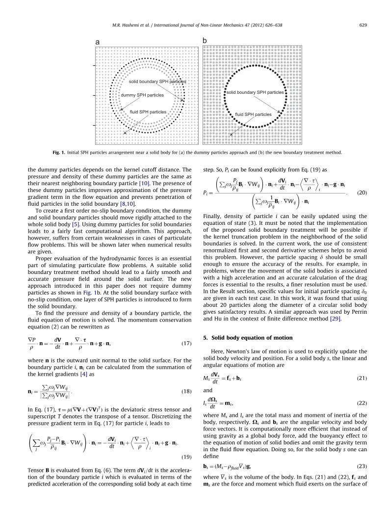
Fig. 1. Initial SPH particles arrangement near a solid body for (a) the dummy particles approach and (b) the new boundary treatment method.

M.R. Hashemi et al. / International Journal of Non-Linear Mechanics 47 (2012) 626–638 629

the dummy particles depends on the kernel cutoff distance. Thepressure and density of these dummy particles are the same astheir nearest neighboring boundary particle [10]. The presence ofthese dummy particles improves approximation of the pressuregradient term in the flow equation and prevents penetration offluid particles in the solid boundary [8,10].

To create a first order no-slip boundary condition, the dummyand solid boundary particles should move rigidly attached to thewhole solid body [5]. Using dummy particles for solid boundariesleads to a fairly fast computational algorithm. This approach,however, suffers from certain weaknesses in cases of particulateflow problems. This will be shown later when numerical resultsare given.

Proper evaluation of the hydrodynamic forces is an essentialpart of simulating particulate flow problems. A suitable solidboundary treatment method should lead to a fairly smooth andaccurate pressure field around the solid surface. The newapproach introduced in this paper does not require dummyparticles as shown in Fig. 1b. At the solid boundary surface withno-slip condition, one layer of SPH particles is introduced to formthe solid boundary.

To find the pressure and density of a boundary particle, thefluid equation of motion is solved. The momentum conservationequation (2) can be rewritten as

rP

r� n¼�

dV

dt� nþr � sr� nþg � n, ð17Þ

where n is the outward unit normal to the solid surface. For theboundary particle i, ni can be calculated from the summation ofthe kernel gradients [4] as

ni ¼

PjojrWij

9P

jojrWij9: ð18Þ

In Eq. (17), s¼ mðrVþðrVÞT Þ is the deviatoric stress tensor andsuperscript T denotes the transpose of a tensor. Discretizing thepressure gradient term in Eq. (17) for particle i, leads to

Xj

oj

Pj�Pi

r ij

Bi � rWij

0@

1A � ni ¼�

dVi

dt� niþ

r � tr

� �i

� niþg � ni:

ð19Þ

Tensor B is evaluated from Eq. (6). The term dVi=dt is the accelera-tion of the boundary particle i which is evaluated in terms of thepredicted acceleration of the corresponding solid body at each time

step. So, Pi can be found explicitly from Eq. (19) as

Pi ¼

Pjoj

Pj

r ij

Bi � rWij

!� niþ

dVi

dt� ni�

r � tr

� �i

� ni�g � ni

Pjoj

1

r ij

Bi � rWij

!� ni

: ð20Þ

Finally, density of particle i can be easily updated using theequation of state (3). It must be noted that the implementationof the proposed solid boundary treatment will be possible ifthe kernel truncation problem in the neighborhood of the solidboundaries is solved. In the current work, the use of consistentrenormalized first and second derivative schemes helps to avoidthis problem. However, the particle spacing d should be smallenough to ensure the accuracy of the results. For example, inproblems, where the movement of the solid bodies is associatedwith a high acceleration and an accurate calculation of the dragforces is essential to the results, a finer resolution must be used.In the Result section, specific values for initial particle spacing d0

are given in each test case. In this work, it was found that usingabout 20 particles along the diameter of a circular solid bodygives satisfactory results. A similar approach was used by Perrinand Hu in the context of finite difference method [29].

5. Solid body equation of motion

Here, Newton’s law of motion is used to explicitly update thesolid body velocity and position. For a solid body s, the linear andangular equations of motion are

MsdVs

dt¼ fsþbs ð21Þ

and

IsdXs

dt¼ms, ð22Þ

where Ms and Is are the total mass and moment of inertia of thebody, respectively. Xs and bs are the angular velocity and bodyforce vectors. It is computationally more efficient that instead ofusing gravity as a global body force, add the buoyancy effect tothe equation of motion of solid bodies and omit the gravity termin the fluid flow equation. Doing so, for the solid body s one candefine

bs ¼ ðMs�rfluidV sÞg, ð23Þ

where V s is the volume of the body. In Eqs. (21) and (22), fs andms are the force and moment which fluid exerts on the surface of

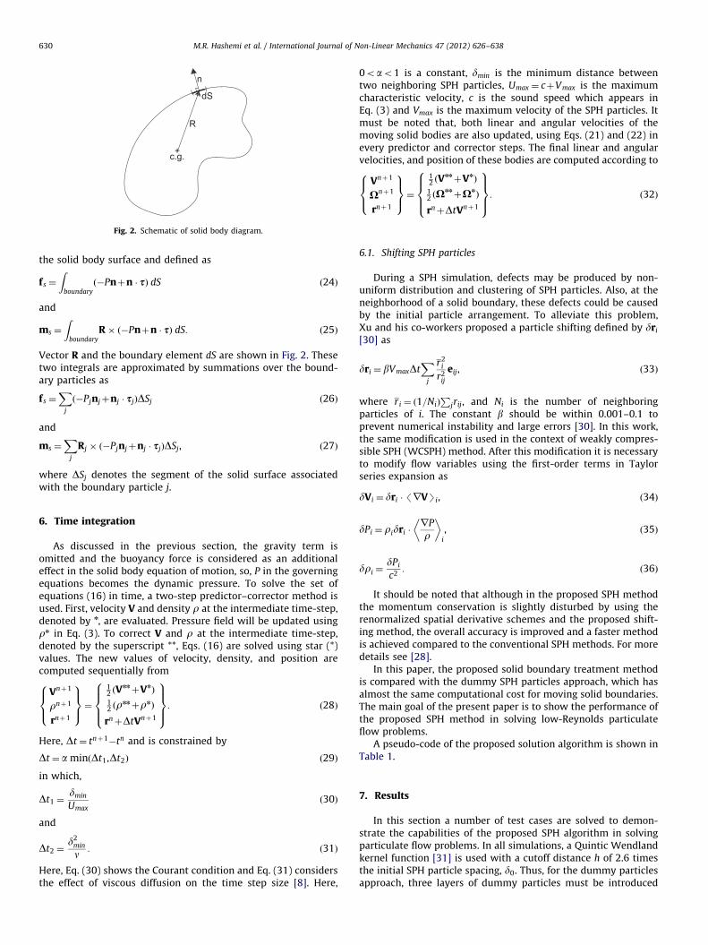
Fig. 2. Schematic of solid body diagram.

M.R. Hashemi et al. / International Journal of Non-Linear Mechanics 47 (2012) 626–638630

the solid body surface and defined as

fs ¼

Zboundary

ð�Pnþn � sÞ dS ð24Þ

and

ms ¼

Zboundary

R � ð�Pnþn � sÞ dS: ð25Þ

Vector R and the boundary element dS are shown in Fig. 2. Thesetwo integrals are approximated by summations over the bound-ary particles as

fs ¼X

j

ð�Pjnjþnj � sjÞDSj ð26Þ

and

ms ¼X

j

Rj � ð�Pjnjþnj � sjÞDSj, ð27Þ

where DSj denotes the segment of the solid surface associatedwith the boundary particle j.

6. Time integration

As discussed in the previous section, the gravity term isomitted and the buoyancy force is considered as an additionaleffect in the solid body equation of motion, so, P in the governingequations becomes the dynamic pressure. To solve the set ofequations (16) in time, a two-step predictor–corrector method isused. First, velocity V and density r at the intermediate time-step,denoted by n, are evaluated. Pressure field will be updated usingrn in Eq. (3). To correct V and r at the intermediate time-step,denoted by the superscript **, Eqs. (16) are solved using star (*)values. The new values of velocity, density, and position arecomputed sequentially from

Vnþ1

rnþ1

rnþ1

8><>:

9>=>;¼

12 ðV

nnþVnÞ

12 ðr

nnþrnÞ

rnþDtVnþ1

8>><>>:

9>>=>>;: ð28Þ

Here, Dt¼ tnþ1�tn and is constrained by

Dt¼ a minðDt1,Dt2Þ ð29Þ

in which,

Dt1 ¼dmin

Umaxð30Þ

and

Dt2 ¼d2

min

n : ð31Þ

Here, Eq. (30) shows the Courant condition and Eq. (31) considersthe effect of viscous diffusion on the time step size [8]. Here,

0oao1 is a constant, dmin is the minimum distance betweentwo neighboring SPH particles, Umax ¼ cþVmax is the maximumcharacteristic velocity, c is the sound speed which appears inEq. (3) and Vmax is the maximum velocity of the SPH particles. Itmust be noted that, both linear and angular velocities of themoving solid bodies are also updated, using Eqs. (21) and (22) inevery predictor and corrector steps. The final linear and angularvelocities, and position of these bodies are computed according to

Vnþ1

Xnþ1

rnþ1

8><>:

9>=>;¼

12 ðV

nnþVnÞ

12 ðX

nnþXn

Þ

rnþDtVnþ1

8>><>>:

9>>=>>;: ð32Þ

6.1. Shifting SPH particles

During a SPH simulation, defects may be produced by non-uniform distribution and clustering of SPH particles. Also, at theneighborhood of a solid boundary, these defects could be causedby the initial particle arrangement. To alleviate this problem,Xu and his co-workers proposed a particle shifting defined by dri

[30] as

dri ¼ bVmaxDtX

j

r2i

r2ij

eij, ð33Þ

where r i ¼ ð1=NiÞP

jrij, and Ni is the number of neighboringparticles of i. The constant b should be within 0.001–0.1 toprevent numerical instability and large errors [30]. In this work,the same modification is used in the context of weakly compres-sible SPH (WCSPH) method. After this modification it is necessaryto modify flow variables using the first-order terms in Taylorseries expansion as

dVi ¼ dri �/rVSi, ð34Þ

dPi ¼ ridri �rP

r

� �i

, ð35Þ

dri ¼dPi

c2: ð36Þ

It should be noted that although in the proposed SPH methodthe momentum conservation is slightly disturbed by using therenormalized spatial derivative schemes and the proposed shift-ing method, the overall accuracy is improved and a faster methodis achieved compared to the conventional SPH methods. For moredetails see [28].

In this paper, the proposed solid boundary treatment methodis compared with the dummy SPH particles approach, which hasalmost the same computational cost for moving solid boundaries.The main goal of the present paper is to show the performance ofthe proposed SPH method in solving low-Reynolds particulateflow problems.

A pseudo-code of the proposed solution algorithm is shown inTable 1.

7. Results

In this section a number of test cases are solved to demon-strate the capabilities of the proposed SPH algorithm in solvingparticulate flow problems. In all simulations, a Quintic Wendlandkernel function [31] is used with a cutoff distance h of 2.6 timesthe initial SPH particle spacing, d0. Thus, for the dummy particlesapproach, three layers of dummy particles must be introduced

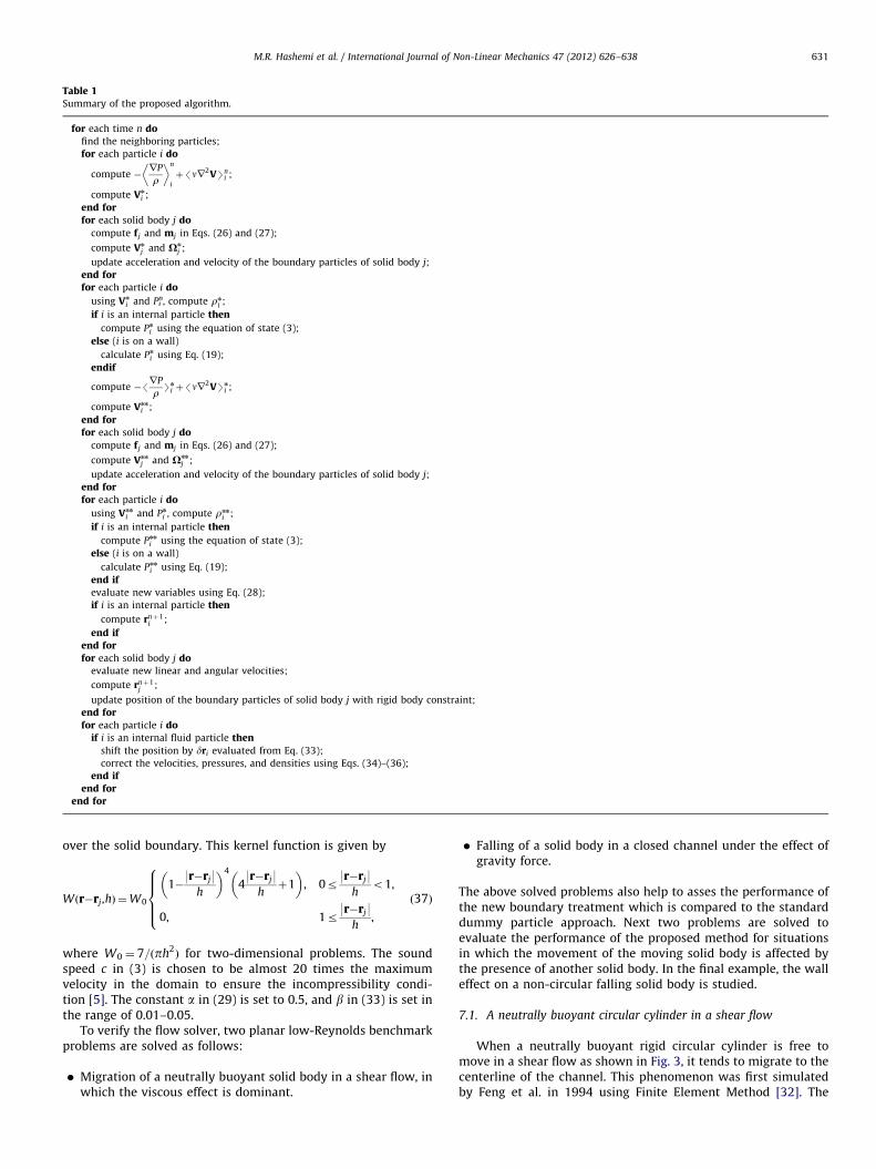
Table 1Summary of the proposed algorithm.

for each time n dofind the neighboring particles;

for each particle i do

compute �rP

r

� �n

i

þ/nr2VSni ;

compute Vn

i ;

end forfor each solid body j do

compute fj and mj in Eqs. (26) and (27);

compute Vn

j and Xn

j ;

update acceleration and velocity of the boundary particles of solid body j;

end forfor each particle i do

using Vn

i and Pin, compute rn

i ;

if i is an internal particle then

compute Pn

i using the equation of state (3);

else (i is on a wall)

calculate Pn

i using Eq. (19);

endif

compute �/rP

rSn

i þ/nr2VSn

i ;

compute Vnn

i ;

end forfor each solid body j do

compute fj and mj in Eqs. (26) and (27);

compute Vnn

j and Xnn

j ;

update acceleration and velocity of the boundary particles of solid body j;

end forfor each particle i do

using Vnn

i and Pn

i , compute rnn

i ;

if i is an internal particle then

compute Pnn

i using the equation of state (3);

else (i is on a wall)

calculate Pnn

i using Eq. (19);

end ifevaluate new variables using Eq. (28);

if i is an internal particle then

compute rnþ1i ;

end ifend forfor each solid body j do

evaluate new linear and angular velocities;

compute rnþ1j ;

update position of the boundary particles of solid body j with rigid body constraint;

end forfor each particle i do

if i is an internal fluid particle then

shift the position by dri evaluated from Eq. (33);

correct the velocities, pressures, and densities using Eqs. (34)–(36);

end ifend for

end for

M.R. Hashemi et al. / International Journal of Non-Linear Mechanics 47 (2012) 626–638 631

over the solid boundary. This kernel function is given by

Wðr�rj,hÞ ¼W0

1�9r�rj9

h

� �4

49r�rj9

hþ1

� �, 0r

9r�rj9h

o1,

0, 1r9r�rj9

h,

8>>><>>>:

ð37Þ

where W0 ¼ 7=ðph2Þ for two-dimensional problems. The sound

speed c in (3) is chosen to be almost 20 times the maximumvelocity in the domain to ensure the incompressibility condi-tion [5]. The constant a in (29) is set to 0.5, and b in (33) is set inthe range of 0.01–0.05.

To verify the flow solver, two planar low-Reynolds benchmarkproblems are solved as follows:

�

Migration of a neutrally buoyant solid body in a shear flow, inwhich the viscous effect is dominant.

�

Falling of a solid body in a closed channel under the effect ofgravity force.

The above solved problems also help to asses the performance ofthe new boundary treatment which is compared to the standarddummy particle approach. Next two problems are solved toevaluate the performance of the proposed method for situationsin which the movement of the moving solid body is affected bythe presence of another solid body. In the final example, the walleffect on a non-circular falling solid body is studied.

7.1. A neutrally buoyant circular cylinder in a shear flow

When a neutrally buoyant rigid circular cylinder is free tomove in a shear flow as shown in Fig. 3, it tends to migrate to thecenterline of the channel. This phenomenon was first simulatedby Feng et al. in 1994 using Finite Element Method [32]. The

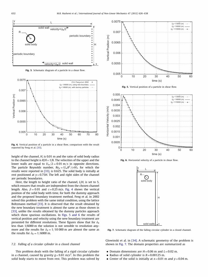
Fig. 3. Schematic diagram of a particle in a shear flow.

0.005

0.0055

0.006

0.0065

0.007

0.0075

0 10 20 30 40 50 60 70 80

Ver

tical

Pos

ition

(m)

time (s)

Fig. 4. Vertical position of a particle in a shear flow, comparison with the result

reported by Feng et al. [33].

0.005

0.0055

0.006

0.0065

0.007

0.0075

0 10 20 30 40 50 60

Ver

tical

Pos

ition

(m)

time (s)

Fig. 5. Vertical position of a particle in shear flow.

0

0.0005

0.001

0.0015

0.002

0.0025

0.003

0.0035

0.004

0.0045

0.005

0 10 20 30 40 50 60

Hor

izon

tal V

eloc

ity (m

/s)

time (s)

Fig. 6. Horizontal velocity of a particle in shear flow.

Fig. 7. Schematic diagram of the falling circular cylinder in a closed channel.

M.R. Hashemi et al. / International Journal of Non-Linear Mechanics 47 (2012) 626–638632

height of the channel, H, is 0.01 m and the ratio of solid body radiusto the channel height is R/H¼1/8. The velocities of the upper and thelower walls are equal to Uw=2¼ 0:01 m=s in opposite directions.The particle Reynolds number, Rep ¼UwR2=ðnHÞ, for which theresults were reported in [33], is 0.625. The solid body is initially atrest positioned at y¼0.75H. The left and right sides of the channelare periodic boundaries.

Here, the length to height ratio of the channel, L/H, is set to 5,which ensures that results are independent from the chosen channellength. Also, b¼ 0:01 and c¼0.25 m/s. Fig. 4 shows the verticalposition of the solid body with time, for both the dummy approachand the proposed boundary treatment method. Feng et al. in 2002solved this problem with the same initial condition, using the latticeBoltzmann method [33]. It is observed that the result obtained bythe new boundary treatment is almost the same as those shown in[33], unlike the results obtained by the dummy particles approachwhich show spurious oscillations. In Figs. 5 and 6 the results ofvertical position and velocity using the new boundary treatment arepresented for different resolutions. These figures show that for d0

less than 1/6000 m the solution is not sensible to resolution any-more and the results for d0 ¼ 1=10 000 m are almost the same asthe results for d0 ¼ 1=6000 m.

7.2. Falling of a circular cylinder in a closed channel

This problem deals with the falling of a rigid circular cylinderin a channel, caused by gravity g¼9.81 m/s2. In this problem thesolid body starts to move from rest. This problem was solved by

Glowinski et al. in [34]. A schematic geometry of the problem isshown in Fig. 7. The domain properties are summarized as

�

Domain dimensions are H¼0.06 m and L¼0.02 m. � Radius of solid cylinder is R¼0.00125 m. � Center of the solid is initially at x¼0.01 m and y¼0.04 m.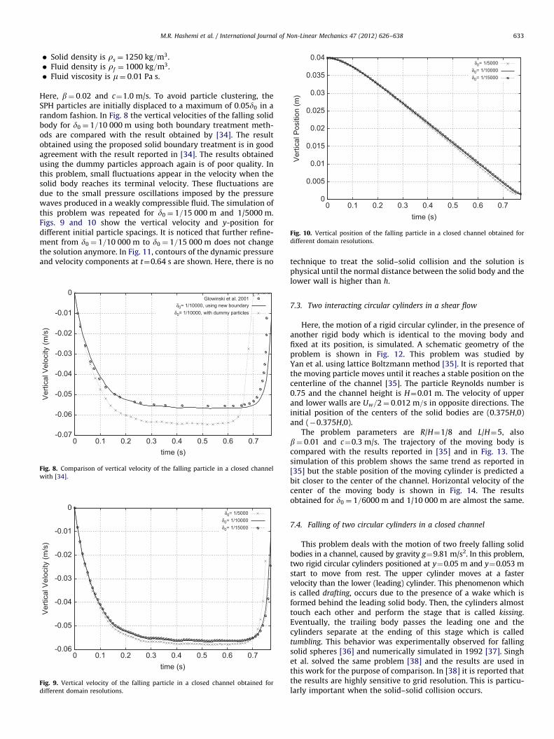

0.04

M.R. Hashemi et al. / International Journal of Non-Linear Mechanics 47 (2012) 626–638 633

�

Ver

tical

Vel

ocity

(m/s

)

Figwit

Ver

tical

Vel

ocity

(m/s

)

Figdiff

Solid density is rs ¼ 1250 kg=m3.

� Fluid density is rf ¼ 1000 kg=m3.

0.035

� Fluid viscosity is m¼ 0:01 Pa s.

0

0.005

0.01

0.015

0.02

0.025

0.03

0 0.1 0.2 0.3 0.4 0.5 0.6 0.7

Ver

tical

Pos

ition

(m)

time (s)

Fig. 10. Vertical position of the falling particle in a closed channel obtained for

different domain resolutions.

Here, b¼ 0:02 and c¼1.0 m/s. To avoid particle clustering, theSPH particles are initially displaced to a maximum of 0:05d0 in arandom fashion. In Fig. 8 the vertical velocities of the falling solidbody for d0 ¼ 1=10 000 m using both boundary treatment meth-ods are compared with the result obtained by [34]. The resultobtained using the proposed solid boundary treatment is in goodagreement with the result reported in [34]. The results obtainedusing the dummy particles approach again is of poor quality. Inthis problem, small fluctuations appear in the velocity when thesolid body reaches its terminal velocity. These fluctuations aredue to the small pressure oscillations imposed by the pressurewaves produced in a weakly compressible fluid. The simulation ofthis problem was repeated for d0 ¼ 1=15 000 m and 1/5000 m.Figs. 9 and 10 show the vertical velocity and y-position fordifferent initial particle spacings. It is noticed that further refine-ment from d0 ¼ 1=10 000 m to d0 ¼ 1=15 000 m does not changethe solution anymore. In Fig. 11, contours of the dynamic pressureand velocity components at t¼0.64 s are shown. Here, there is no

-0.07

-0.06

-0.05

-0.04

-0.03

-0.02

-0.01

0

0 0.1 0.2 0.3 0.4 0.5 0.6 0.7time (s)

. 8. Comparison of vertical velocity of the falling particle in a closed channel

h [34].

-0.06

-0.05

-0.04

-0.03

-0.02

-0.01

0

0 0.1 0.2 0.3 0.4 0.5 0.6 0.7time (s)

. 9. Vertical velocity of the falling particle in a closed channel obtained for

erent domain resolutions.

technique to treat the solid–solid collision and the solution isphysical until the normal distance between the solid body and thelower wall is higher than h.

7.3. Two interacting circular cylinders in a shear flow

Here, the motion of a rigid circular cylinder, in the presence ofanother rigid body which is identical to the moving body andfixed at its position, is simulated. A schematic geometry of theproblem is shown in Fig. 12. This problem was studied byYan et al. using lattice Boltzmann method [35]. It is reported thatthe moving particle moves until it reaches a stable position on thecenterline of the channel [35]. The particle Reynolds number is0.75 and the channel height is H¼0.01 m. The velocity of upperand lower walls are Uw=2¼ 0:012 m=s in opposite directions. Theinitial position of the centers of the solid bodies are (0.375H,0)and (�0.375H,0).

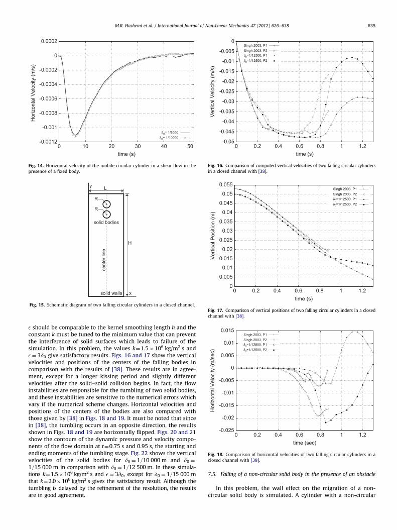
The problem parameters are R/H¼1/8 and L/H¼5, alsob¼ 0:01 and c¼0.3 m/s. The trajectory of the moving body iscompared with the results reported in [35] and in Fig. 13. Thesimulation of this problem shows the same trend as reported in[35] but the stable position of the moving cylinder is predicted abit closer to the center of the channel. Horizontal velocity of thecenter of the moving body is shown in Fig. 14. The resultsobtained for d0 ¼ 1=6000 m and 1/10 000 m are almost the same.

7.4. Falling of two circular cylinders in a closed channel

This problem deals with the motion of two freely falling solidbodies in a channel, caused by gravity g¼9.81 m/s2. In this problem,two rigid circular cylinders positioned at y¼0.05 m and y¼0.053 mstart to move from rest. The upper cylinder moves at a fastervelocity than the lower (leading) cylinder. This phenomenon whichis called drafting, occurs due to the presence of a wake which isformed behind the leading solid body. Then, the cylinders almosttouch each other and perform the stage that is called kissing.Eventually, the trailing body passes the leading one and thecylinders separate at the ending of this stage which is calledtumbling. This behavior was experimentally observed for fallingsolid spheres [36] and numerically simulated in 1992 [37]. Singhet al. solved the same problem [38] and the results are used inthis work for the purpose of comparison. In [38] it is reported thatthe results are highly sensitive to grid resolution. This is particu-larly important when the solid–solid collision occurs.

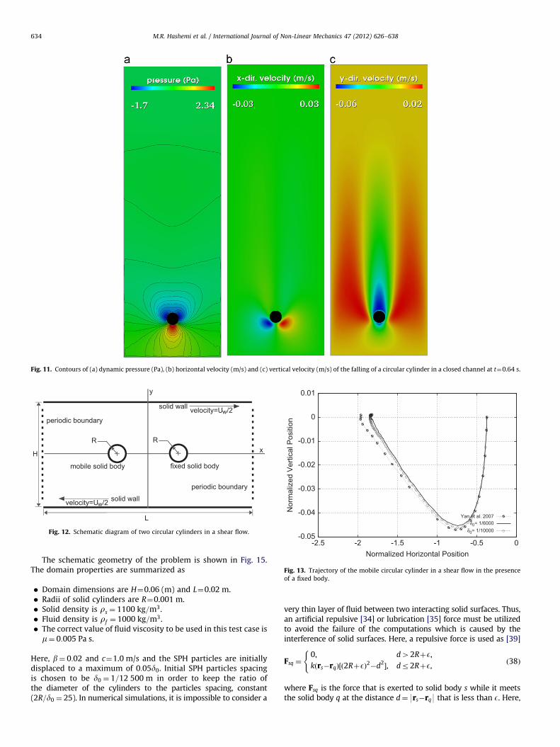
Fig. 11. Contours of (a) dynamic pressure (Pa), (b) horizontal velocity (m/s) and (c) vertical velocity (m/s) of the falling of a circular cylinder in a closed channel at t¼0.64 s.

Fig. 12. Schematic diagram of two circular cylinders in a shear flow. -0.05

-0.04

-0.03

-0.02

-0.01

0

0.01

-2.5 -2 -1.5 -1 -0.5 0

Nor

mal

ized

Ver

tical

Pos

ition

Normalized Horizontal Position

Fig. 13. Trajectory of the mobile circular cylinder in a shear flow in the presence

M.R. Hashemi et al. / International Journal of Non-Linear Mechanics 47 (2012) 626–638634

The schematic geometry of the problem is shown in Fig. 15.The domain properties are summarized as

of a fixed body.

�

Domain dimensions are H¼0.06 (m) and L¼0.02 m. � Radii of solid cylinders are R¼0.001 m. � Solid density is rs ¼ 1100 kg=m3. � Fluid density is rf ¼ 1000 kg=m3. � The correct value of fluid viscosity to be used in this test case ism¼ 0:005 Pa s.

Here, b¼ 0:02 and c¼1.0 m/s and the SPH particles are initiallydisplaced to a maximum of 0:05d0. Initial SPH particles spacingis chosen to be d0 ¼ 1=12 500 m in order to keep the ratio ofthe diameter of the cylinders to the particles spacing, constant(2R=d0 ¼ 25). In numerical simulations, it is impossible to consider a

very thin layer of fluid between two interacting solid surfaces. Thus,an artificial repulsive [34] or lubrication [35] force must be utilizedto avoid the failure of the computations which is caused by theinterference of solid surfaces. Here, a repulsive force is used as [39]

Fsq ¼0, d42RþE,kðrs�rqÞ½ð2RþEÞ2�d2

�, dr2RþE,

(ð38Þ

where Fsq is the force that is exerted to solid body s while it meetsthe solid body q at the distance d¼ 9rs�rq9 that is less than E. Here,

-0.0012

-0.001

-0.0008

-0.0006

-0.0004

-0.0002

0

0.0002

0 10 20 30 40 50

Hor

izon

tal V

eloc

ity (m

/s)

time (s)

Fig. 14. Horizontal velocity of the mobile circular cylinder in a shear flow in the

presence of a fixed body.

Fig. 15. Schematic diagram of two falling circular cylinders in a closed channel.

-0.05

-0.045

-0.04

-0.035

-0.03

-0.025

-0.02

-0.015

-0.01

-0.005

0

0 0.2 0.4 0.6 0.8 1 1.2

Ver

tical

Vel

ocity

(m/s

)

time (s)

Fig. 16. Comparison of computed vertical velocities of two falling circular cylinders

in a closed channel with [38].

0

0.005

0.01

0.015

0.02

0.025

0.03

0.035

0.04

0.045

0.05

0.055

0 0.2 0.4 0.6 0.8 1 1.2

Ver

tical

Pos

ition

(m)

time (s)

Fig. 17. Comparison of vertical positions of two falling circular cylinders in a closed

channel with [38].

-0.025

-0.02

-0.015

-0.01

-0.005

0

0.005

0.01

0.015

0 0.2 0.4 0.6 0.8 1 1.2

Hor

izon

tal V

eloc

ity (m

/sec

)

time (sec)

Fig. 18. Comparison of horizontal velocities of two falling circular cylinders in a

closed channel with [38].

M.R. Hashemi et al. / International Journal of Non-Linear Mechanics 47 (2012) 626–638 635

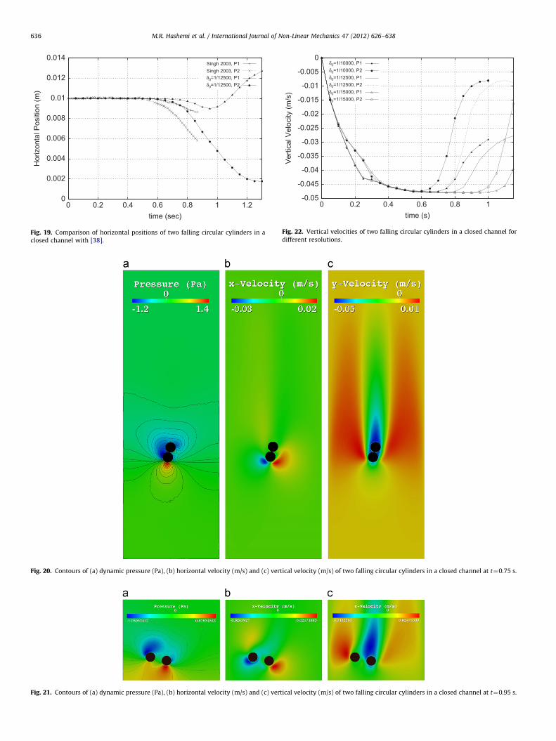
E should be comparable to the kernel smoothing length h and theconstant k must be tuned to the minimum value that can preventthe interference of solid surfaces which leads to failure of thesimulation. In this problem, the values k¼1.5�106 kg/m2 s andE¼ 3d0 give satisfactory results. Figs. 16 and 17 show the verticalvelocities and positions of the centers of the falling bodies incomparison with the results of [38]. These results are in agree-ment, except for a longer kissing period and slightly differentvelocities after the solid–solid collision begins. In fact, the flowinstabilities are responsible for the tumbling of two solid bodies,and these instabilities are sensitive to the numerical errors whichvary if the numerical scheme changes. Horizontal velocities andpositions of the centers of the bodies are also compared withthose given by [38] in Figs. 18 and 19. It must be noted that sincein [38], the tumbling occurs in an opposite direction, the resultsshown in Figs. 18 and 19 are horizontally flipped. Figs. 20 and 21show the contours of the dynamic pressure and velocity compo-nents of the flow domain at t¼0.75 s and 0.95 s, the starting andending moments of the tumbling stage. Fig. 22 shows the verticalvelocities of the solid bodies for d0 ¼ 1=10 000 m and d0 ¼

1=15 000 m in comparison with d0 ¼ 1=12 500 m. In these simula-tions k¼1.5�106 kg/m2 s and E¼ 3d0, except for d0 ¼ 1=15 000 mthat k¼2.0�106 kg/m2 s gives the satisfactory result. Although thetumbling is delayed by the refinement of the resolution, the resultsare in good agreement.

7.5. Falling of a non-circular solid body in the presence of an obstacle

In this problem, the wall effect on the migration of a non-circular solid body is simulated. A cylinder with a non-circular

0

0.002

0.004

0.006

0.008

0.01

0.012

0.014

0 0.2 0.4 0.6 0.8 1 1.2

Hor

izon

tal P

ositi

on (m

)

time (sec)

Fig. 19. Comparison of horizontal positions of two falling circular cylinders in a

closed channel with [38].

Fig. 20. Contours of (a) dynamic pressure (Pa), (b) horizontal velocity (m/s) and (c) vertical velocity (m/s) of two falling circular cylinders in a closed channel at t¼0.75 s.

Fig. 21. Contours of (a) dynamic pressure (Pa), (b) horizontal velocity (m/s) and (c) vertical velocity (m/s) of two falling circular cylinders in a closed channel at t¼0.95 s.

-0.05

-0.045

-0.04

-0.035

-0.03

-0.025

-0.02

-0.015

-0.01

-0.005

0

0 0.2 0.4 0.6 0.8 1

Ver

tical

Vel

ocity

(m/s

)

time (s)

Fig. 22. Vertical velocities of two falling circular cylinders in a closed channel for

different resolutions.

M.R. Hashemi et al. / International Journal of Non-Linear Mechanics 47 (2012) 626–638636

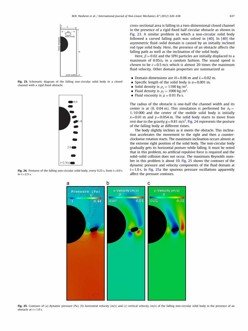
Fig. 23. Schematic diagram of the falling non-circular solid body in a closed

channel with a rigid fixed obstacle.

Fig. 24. Postures of the falling non-circular solid body, every 0.25 s, from t¼0.0 s

to t¼2.5 s.

Fig. 25. Contours of (a) dynamic pressure (Pa), (b) horizontal velocity (m/s) and (c) v

obstacle at t¼1.0 s.

M.R. Hashemi et al. / International Journal of Non-Linear Mechanics 47 (2012) 626–638 637

cross-sectional area is falling in a two-dimensional closed channelin the presence of a rigid fixed half circular obstacle as shown inFig. 23. A similar problem in which a non-circular solid bodyfollowed a curved falling path was solved in [40]. In [40] theasymmetric fluid–solid domain is caused by an initially inclinedrod type solid body. Here, the presence of an obstacle affects thefalling path as well as the inclination of the solid body.

Here, b¼ 0:02 and the SPH particles are initially displaced to amaximum of 0:05d0 in a random fashion. The sound speed ischosen to be c¼0.5 m/s which is almost 20 times the maximumfluid velocity. Other domain properties are summarized as

�

erti

Domain dimensions are H¼0.06 m and L¼0.02 m.

� Specific length of the solid body is a¼0.001 m. � Solid density is rs ¼ 1100 kg=m3. � Fluid density is rf ¼ 1000 kg=m3. � Fluid viscosity is m¼ 0:01 Pa s.

The radius of the obstacle is one-half the channel width and itscenter is at (0, 0.04 m). This simulation is performed for d0 ¼

1=10 000 and the center of the mobile solid body is initiallyx¼0.01 m and y¼0.054 m. The solid body starts to move fromrest due to the gravity g¼9.81 m/s2. Fig. 24 represents the postureof the falling body at different times.

The body slightly inclines as it meets the obstacle. This inclina-tion accelerates the movement to the right and then a counter-clockwise rotation starts. The maximum inclination occurs almost atthe extreme right position of the solid body. The non-circular bodygradually gets its horizontal posture while falling. It must be notedthat in this problem, no artificial repulsive force is required and thesolid–solid collision does not occur. The maximum Reynolds num-ber in this problem is about 10. Fig. 25 shows the contours of thedynamic pressure and velocity components of the fluid domain att¼1.0 s. In Fig. 25a the spurious pressure oscillations apparentlyaffect the pressure contours.

cal velocity (m/s) of the falling non-circular solid body in the presence of an

M.R. Hashemi et al. / International Journal of Non-Linear Mechanics 47 (2012) 626–638638

8. Conclusions

A modified SPH method was presented to simulate particulateflow problems. Solving a number of benchmark problems, theproposed method proved to be robust and more stable in the sensethat no artificial viscosity was used to obtain solutions for theproblems solved in this paper. The newly proposed solid boundarytreatment helped to greatly improve the pressure distribution onthe solid boundary. It also showed significant improvement in theresults in comparison with the dummy particle technique.

Using a relatively higher value for the tuning parameter in theSPH shifting method, the method was able to handle higherReynolds flow problems. It should be noted, however, that thisparameter should be increased carefully as it can cause too muchnumerical errors.

Referring to the particulate problems solved in this paper, itcan be concluded that

�

Using a simple repulsive force helped prevent non-physicalsolid–solid collisions and to obtain acceptable results for thefalling problem of two circular cylinders. It is believed that aproper solid–solid collision treatment can enhance the cap-ability of the method for solving many-body problems. � The present method was not tested against solid bodies with

sharp corners. Solving such problems requires further detailedinvestigation to avoid clustering of particles near sharp corners.

References

[1] L.B. Lucy, A numerical approach to the testing of fission hypothesis, Astro-physical Journal 82 (1977) 1013–1020.

[2] R.A. Gingold, J.J. Monaghan, Smoothed particle hydrodynamics: theory andapplication to nonspherical stars, Astrophysical Journal 181 (1977) 275–389.

[3] J.J. Monaghan, Smoothed particle hydrodynamics, Reports on Progress inPhysics 68 (2005) 1703–1759.

[4] P.W. Randles, L.D. Libersky, Smoothed particle hydrodynamics: some recentimprovements and applications, Computer Methods in Applied Mechanicsand Engineering 139 (1–4) (1996) 375–408.

[5] J.P. Morris, P.J. Fox, Y. Zhu, Modeling low Reynolds number incompressibleflows using SPH, Journal of Computational Physics 136 (1) (1997) 214–226.

[6] J.J. Monaghan, Simulating free surface flows with SPH, Journal of Computa-tional Physics 110 (1994) 399–406.

[7] S.J. Cummins, M. Rudman, An SPH projection method, Journal of Computa-tional Physics 152 (2) (1999) 584–607.

[8] S. Shao, E.Y.M. Lo, Incompressible SPH method for simulating newtonian andnon-newtonian flows with a free surface, Advances in Water Resources 26 (7)(2003) 787–800.

[9] S.M. Hosseini, M.T. Manzari, S.K. Hannani, A fully explicit three-step SPHalgorithm for simulation of non-Newtonian fluid flow, International Journalof Numerical Methods for Heat and Fluid Flow 17 (7) (2007) 715–735.

[10] E.S. Lee, C. Moulinec, R. Xu, D. Violeau, D. Laurence, P. Stansby, Comparisonsof weakly compressible and truly incompressible algorithms for the SPHmesh free particle method, Journal of Computational Physics 227 (10) (2008)8417–8436.

[11] A. Potapov, M. Hunt, C. Campbell, Liquid-solid flows using smoothed particlehydrodynamics and the discrete element method, Powder Technology 116(2–3) (2001) 204–213.

[12] A. Colagrossi, M. Landrini, Numerical simulation of interfacial flows bysmoothed particle hydrodynamics, Journal of Computational Physics 191(2) (2003) 448–475.

[13] G. Oger, M. Doring, B. Alessandrini, P. Ferrant, Two-dimensional SPH simula-tions of wedge water entries, Journal of Computational Physics 213 (2)(2006) 803–822.

[14] S. Shao, Incompressible SPH simulation of water entry of a free-fallingobject, International Journal for Numerical Methods in Fluids 59 (1) (2009)91–115.

[15] J. Monaghan, J. Kajtar, SPH particle boundary forces for arbitrary boundaries,Computer Physics Communications 180 (10) (2009) 1811–1820.

[16] M. Liu, G. Liu, Smoothed particle hydrodynamics: an overview and recentdevelopments, Archives of Computational Methods in Engineering 17 (1)(2010) 25–76.

[17] J. Monaghan, A. Kos, N. Issa, Fluid motion generated by impact, Journal ofWaterway, Port, Coastal, and Ocean Engineering 129 (2003) 250.

[18] J. Kajtar, J.J. Monaghan, SPH simulations of swimming linked bodies, Journalof Computational Physics 227 (19) (2008) 8568–8587.

[19] R. Fatehi, M. Manzari, Error estimation in smoothed particle hydrodynamicsand a new scheme for second derivatives, Computers & Mathematics withApplications 61 (2) (2011) 482–498.

[20] R. Fatehi, M. Manzari, A remedy for numerical oscillations in weaklycompressible smoothed particle hydrodynamics, International Journal forNumerical Methods in Fluids 67 (9) (2011) 1100–1114.

[21] N.J. Quinlan, M. Basa, M. Lastiwka, Truncation error in mesh-free particlemethods, International Journal for Numerical Methods in Engineering 66 (13)(2006) 2064–2085.

[22] T. Belytschko, Y. Krongauz, D. Organ, M. Fleming, P. Krysl, Meshless methods:an overview and recent developments, Computer Methods in AppliedMechanics and Engineering 139 (1–4) (1996) 3–47.

[23] J. Bonet, T.S.L. Lok, Variational and momentum preservation aspects ofsmooth particle hydrodynamic formulations, Computer Methods in AppliedMechanics and Engineering 180 (1–2) (1999) 97–115.

[24] J.P. Vila, On particle weighted methods and smooth particle hydrodynamics,Mathematical Models and Methods in Applied Sciences 9 (2) (1999)161–210.

[25] M. Basa, N.J. Quinlan, M. Lastiwka, Robustness and accuracy of SPH formula-tions for viscous flow, International Journal for Numerical Methods in Fluids60 (2009) 1127–1148.

[26] J.H. Ferziger, M. Peric, Computational Methods for Fluid Dynamics, Springer,2002.

[27] C.M. Rhie, W.L. Chow, Numerical study of the turbulent flow past an airfoilwith trailing edge separation, AIAA Journal 21 (11) (1983) 1525–1532.

[28] R. Fatehi, M. Manzari, A consistent and fast weakly compressible smoothedparticle hydrodynamics with a new wall boundary condition, InternationalJournal for Numerical Methods in Fluids, in press, doi: 10.1002/fld.2586.

[29] A. Perrin, H. Hu, An explicit finite-difference scheme for simulation of movingparticles, Journal of Computational Physics 212 (1) (2006) 166–187.

[30] R. Xu, P. Stansby, D. Laurence, Accuracy and stability in incompressible SPH(ISPH) based on the projection method and a new approach, Journal ofComputational Physics 228 (18) (2009) 6703–6725.

[31] H. Wendland, Piecewise polynomial, positive definite and compactly sup-ported radial functions of minimal degree, Advances in ComputationalMathematics 4 (1) (1995) 389–396.

[32] J. Feng, H. Hu, D. Joseph, Direct simulation of initial value problems for themotion of solid bodies in a Newtonian fluid. Part 2. Couette and Poiseuilleflows, Journal of Fluid Mechanics 277 (1994) 271–301.

[33] Z. Feng, E. Michaelides, Interparticle forces and lift on a particle attached to asolid boundary in suspension flow, Physics of Fluids 14 (2002) 49.

[34] R. Glowinski, T. Pan, T. Hesla, D. Joseph, J. Periaux, A distributed Lagrangemultiplier/fictitious domain method for the simulation of flow aroundmoving rigid bodies: application to particulate flow, Journal of Computa-tional Physics 169 (2) (2001) 363–426.

[35] Y. Yan, J. Morris, J. Koplik, Hydrodynamic interaction of two particles inconfined linear shear flow at finite Reynolds number, Physics of Fluids 19(2007) 113305.

[36] A.F. Fortes, D.D. Joseph, T.S. Lundgren, Nonlinear mechanics of fluidization ofbeds of spherical particles, Journal of Fluid Mechanics Digital Archive 177 (1)(1987) 467–483.

[37] H. Hu, D. Joseph, M. Crochet, Direct simulation of fluid particle motions,Theoretical and Computational Fluid Dynamics 3 (5) (1992) 285–306.

[38] P. Singh, T. Hesla, D. Joseph, Distributed Lagrange multiplier method forparticulate flows with collisions, International Journal of Multiphase Flow 29(3) (2003) 495–509.

[39] Z. Zhang, A. Prosperetti, A method for particle simulation, Journal of AppliedMechanics 70 (2003) 64.

[40] T. Lee, Y. Chang, J. Choi, D. Kim, W. Liu, Y. Kim, Immersed finite elementmethod for rigid body motions in the incompressible Navier–Stokes flow,Computer Methods in Applied Mechanics and Engineering 197 (25–28)(2008) 2305–2316.