experimental and analytical investigations of the thermal

EXPERIMENTAL AND ANALYTICAL INVESTIGATIONS OF THE

THERMAL BEHAVIOR OF PRESTRESSED CONCRETE BRIDGE

GIRDERS INCLUDING IMPERFECTIONS

A Thesis Presented to

The Academic Faculty

by

Jong-Han Lee

In Partial Fulfillment of the Requirements for the Degree

Doctor of Philosophy in the School of Civil and Environmental Engineering

Georgia Institute of Technology Atlanta, GA

August 2010

Copyright © 2010 by Jong-Han Lee

EXPERIMENTAL AND ANALYTICAL INVESTIGATIONS OF THE

THERMAL BEHAVIOR OF PRESTRESSED CONCRETE BRIDGE

GIRDERS INCLUDING IMPERFECTIONS

Approved by:

Dr. Kenneth M. Will, Chairman School of Civil and Environmental Engineering Georgia Institute of Technology

Dr. Leroy Z. Emkin School of Civil and Environmental Engineering Georgia Institute of Technology

Dr. Lawrence F. Kahn School of Civil and Environmental Engineering Georgia Institute of Technology

Dr. Yogendra Joshi School of Mechanical Engineering Georgia Institute of Technology

Dr. Abdul-Hamid Zureick School of Civil and Environmental Engineering Georgia Institute of Technology

Data Approved: [ 7/01/2010 ]

iii

ACKNOWLEDGEMENTS

First and foremost, I would like to gratefully and sincerely thank my advisor, Dr.

Kenneth M. Will, for his unwavering support, guidance, and understanding relating to

various matters during my research. His profound knowledge and his invaluable insights

into structural concepts and physical behaviors helped me enhance my knowledge of

structural engineering, a goal that I wished to attain during my Ph.D. studies. I would

also like to express my gratitude to Dr. Lawrence F. Kahn for his support and advice on

my research and special thanks for his assistance and input about the difficulties and

situations that could be ignored in my experiment. I would also like to extend my

gratitude to the members of my thesis committee—Dr. Abdul-Hamid Zureick, Dr. Leroy

Emkin, and Dr. Yogendra Joshi—for their comments and advice on the completion of my

dissertation.

I would also like to express my deepest appreciation to Dr. Yong Myung Park for

his unfailing attention to my studies and his profound belief in my abilities. I’d also like

to express my gratitude to Dr. Chung Bang Yun for his attention and advice over the

years. I would also like to take this opportunity to thank all the members of the Structural

Dynamics Laboratory at the Korea Advanced Institute of Science and Technology for

their encouragement.

Thanks also to all of my fellow students, laboratory technicians, and friends in the

School of Civil and Environmental Engineering at Georgia Tech for their kind words and

friendly support when needed. I also have had great the pleasure of working with my

office mates, Ben Deaton, Murat Efe Guney, Mustafa Can Kara, Jennifer Modugno, and

iv

Jennifer Dunbeck, and with all the members of the Computer-Aided Structural

Engineering Center at Georgia Institute of Technology for the past five years.

Finally, and most importantly, I wish to thank my parents and my sister for their

love and support. I am particularly extremely grateful to my mom for her endless support

and love. A special thank to my wife, Kyung Hye, for her continuous encouragement and

unwavering belief when it was most required through the completion of my degree.

v

TABLE OF CONTENTS

ACKNOWLEDGEMENTS ............................................................................................... iii

LIST OF TABLES .............................................................................................................. x

LIST OF FIGURES ........................................................................................................ xiv

LIST OF SYMBOLS ..................................................................................................... xxxi

LIST OF ABBREVIATIONS ........................................................................................xxxv

SUMMARY .............................................................................................................. xxxvi

CHAPTER 1 INTRODUCTION ........................................................................................ 1

1.1 Problem Description ........................................................................................... 1

1.2 Previous Studies ................................................................................................. 3

1.2.1 Environmental Thermal Effects in Concrete Bridges............................. 4

1.2.2 Girder Sweep and Support Conditions in Prestressed Concrete Girders .. 15

1.3 Research Scope and Objectives ........................................................................ 19

1.4 Overview and Structure of the Thesis .............................................................. 20

CHAPTER 2 EXPERIMENTAL INVESTIGATION OF THERMAL EFFECTS ........... 22

2.1 Introduction ...................................................................................................... 22

2.2 Specimen Preparation ....................................................................................... 22

2.3 Instrumentation ................................................................................................. 24

2.3.1 Environmental Variables ...................................................................... 25

2.3.2 Girder Temperatures ............................................................................. 26

2.3.3 Data Acquisition Systems ..................................................................... 28

2.4 Measurements of Environmental Conditions and Girder Temperatures .......... 29

vi

2.4.1 Environmental Conditions .................................................................... 29

2.4.2 Girder Temperatures ............................................................................. 36

2.5 Variations in Vertical and Transverse Temperature Differences....................... 43

2.5.1 Vertical Temperature Differences ......................................................... 43

2.5.2 Transverse Temperature Differences .................................................... 46

2.6 Variations in Vertical and Transverse Temperature Distributions and Gradients .. 51

2.6.1 Vertical Temperature Distributions and Gradients ............................... 51

2.6.2 Transverse Temperature Distributions and Gradients .......................... 54

CHAPTER 3 FINITE ELEMENT HEAT TRANSFER MODEL .................................... 61

3.1 Introduction ...................................................................................................... 61

3.2 Calculation of Solar Energy on the Inclined Surfaces ...................................... 61

3.3 Transient Heat Transfer Analysis ..................................................................... 66

3.3.1 Heat Conduction ................................................................................... 67

3.3.2 Heat Convection ................................................................................... 67

3.3.3 Heat Irradiation and Radiation ............................................................. 68

3.4 Analytical Results ............................................................................................. 69

3.4.1 Vertical and Transverse Temperature Variations .................................. 70

3.4.2 Vertical and Transverse Temperature Differences ................................ 76

3.4.3 Vertical and Transverse Temperature Distributions ............................. 77

CHAPTER 4 THERMAL RESPONSE ANALYSIS ........................................................ 85

4.1 Introduction ...................................................................................................... 85

4.2 3D Finite Element Model ................................................................................. 85

4.2.1 The Model of Concrete Girder and Prestressing Strands ..................... 85

vii

4.2.2 Support Boundary Conditions .............................................................. 89

4.2.3 Concrete and Prestressing Strand Material Properties ......................... 90

4.3 Thermal Response Analysis ............................................................................. 93

4.3.1 Sequence Analysis Procedures ............................................................. 93

4.3.2 Thermal Movements ............................................................................. 94

4.3.3 Thermal Stresses ................................................................................. 100

CHAPTER 5 DESIGN THERMAL GRADIENTS IN PRESTRESSED CONCRETE

BRIDGE GIRDERS ................................................................................. 109

5.1 Introduction .................................................................................................... 109

5.2 Extreme Seasonal Daily Environmental Conditions ...................................... 109

5.2.1 Solar Radiation ....................................................................................110

5.2.2 Air Temperature ................................................................................... 111

5.2.3 Wind Speed .........................................................................................114

5.3 Hourly Variations in Seasonal Environmental Conditions ..............................114

5.3.1 Solar Radiation ....................................................................................116

5.3.2 Air Temperature .................................................................................. 121

5.4 Extreme Seasonal Girder Temperature Variations .......................................... 124

5.4.1 Finite Element Transient Heat Transfer Analysis ............................... 124

5.4.2 Time Interval and Period of the Heat Transfer Analysis .................... 128

5.4.3 Seasonal Temperature Differentials.................................................... 131

5.4.4 Seasonal Vertical Temperature Distributions ..................................... 139

5.4.5 Seasonal Transverse Temperature Distributions ................................ 145

5.5 Influences of Bridge Axes on the Temperature Distributions ........................ 150

viii

5.5.1 Vertical Temperature Differentials and Gradients .............................. 151

5.5.2 Transverse Temperature Differentials and Gradients in the Top Flange . 154

5.5.3 Transverse Temperature Differentials and Gradients in the Web ....... 158

5.5.4 Transverse Temperature Differentials and Gradients in the Bottom

Flange ................................................................................................. 162

5.6 Thermal Differentials at Selected Cities in the United States ........................ 166

5.6.1 Extreme Environmental Conditions in the United States ................... 166

5.6.2 Vertical and Transverse Temperature Differentials ............................ 169

CHAPTER 6 STRUCTURAL BEHAVIOR OF A PRESTRESSED CONCRETE

BRIDGE GIRDER DURING CONSTRUCTION ................................... 173

6.1 Introduction .................................................................................................... 173

6.2 3D Finite Element Thermal Response Analysis ............................................. 173

6.2.1 Finite Element Model of the Prestressed Concrete BT-63 Girder ...... 174

6.2.2 Support Conditions ............................................................................. 177

6.2.3 Thermal Movements ........................................................................... 183

6.2.4 Thermal Stresses ................................................................................. 189

6.3 Behavior of a Prestressed Concrete Girder During Construction .................. 192

6.3.1 Procedures of Sequential Analyses ..................................................... 192

6.3.2 Structural Analyses with Support Slope and Initial Sweep ................ 195

6.3.3 Vertical Behavior of the Prestressed Concrete Girder ........................ 196

6.3.4 Transverse Behavior of the Prestressed Concrete Girder ................... 201

6.4 A Simple Beam Model for the Calculation of Thermal Deformations .......... 206

6.4.1 Development of the Simple Beam Model .......................................... 206

ix

6.4.2 Comparison of the Beam Model with the 3D Finite Element Analysis . 210

6.4.3 Thermal Movements of AASHTO-PCI Bridge Girders ..................... 213

CHAPTER 7 INFLUENCES OF THE THERMAL PROPERTIES ON TEMPERATURE

DISTRIBUTIONS AND THERMAL BEHAVIOR ................................. 215

7.1 Introduction .................................................................................................... 215

7.2 Literature Reviews on the Thermal Properties of Concrete ........................... 215

7.2.1 Thermal Conductivity and Specific Heat ........................................... 216

7.2.2 Solar Absorptivity ............................................................................... 217

7.2.3 Thermal Expansion Coefficient .......................................................... 217

7.3 Temperature Distributions with the Thermal Properties of Concrete............. 218

7.3.1 Thermal Conductivity of Concrete ..................................................... 218

7.3.2 Specific Heat of Concrete ................................................................... 228

7.3.3 Solar Absorptivity of Concrete ........................................................... 231

7.3.4 The Rate of Temperature Changes with the Thermal Properties of

Concrete .............................................................................................. 234

7.4 Thermal Movements with the Coefficient of Thermal Expansion (CTE) ...... 237

CHAPTER 8 CONCLUSIONS AND RECOMMENDATIONS .................................... 241

8.1 Conclusions .................................................................................................... 241

8.2 Recommendations for Future Studies ............................................................ 245

APPENDIX A: A MODEL OF TRANSFER TEMPERATURE DISTRIBUTION .....246

APPENDIX B: CALCULATION OF SOLAR POSITION ..........................................249

APPENDIX C: CALCULATION OF SOLAR POSITION ..........................................252

REFERENCES ................................................................................................................258

VITA ................................................................................................................................265

x

LIST OF TABLES

Table 1.1: Correlation between the effective bridge temperatures and normal daily air

temperatures (AASHTO, 1989)..................................................................... 13

Table 2.1: The daily environmental conditions for selected sunny days during the

measurements from April 2009 to March 2010. ............................................ 30

Table 2.2: Solar radiation measured on the horizontal and vertical surfaces on June 1,

October 1, and November 15, 2009. ............................................................. 31

Table 2.3: The highest daily girder temperatures and the daily vertical temperature

differences for selected sunny days during the months of April 2009 to March

2010. .............................................................................................................. 45

Table 2.4: The daily transverse temperature differences in the top flange, the web, and

the bottom flange for selected sunny days during the months of April 2009 to

March 2010. ................................................................................................... 50

Table 3.1: Average absolute errors between the predicted and measured temperatures at

each sensor location on June 1 and November 15, 2009. .............................. 75

Table 3.2: Comparison between the predicted and measured maximum vertical and

transverse temperature differences on June 1, 2009. ..................................... 77


transverse temperature differences on November 15, 2009. ......................... 77

Table 4.1: The material properties of concrete for the thermal response analysis. ......... 91

Table 4.2: The material properties of strands for the thermal response analysis. ........... 92

xi

Table 4.3: The maximum thermal movements of the BT-63 girder on June 1 and

November 15, 2009. ...................................................................................... 95

Table 5.1: Monthly average solar radiation on a horizontal surface extracted from the

NSRDB data and measured during the months of April 2009 to March 2010. ... 111

Table 5.2: Monthly average daily air temperatures extracted from the NCDC data and

measured during the months of April 2009 to March 2010. ........................113

Table 5.3: Seasonal largest vertical temperature differentials along the depth (A-A) of

the four AASHTO-PCI standard girder sections. ........................................ 134

Table 5.4: Seasonal largest transverse temperature differentials in the top flange (B-B),

in the web (C-C), and the bottom flange (D-D) of the four AASHTO-PCI

standard girder sections. .............................................................................. 134

Table 5.5: Seasonal largest vertical temperature differentials in Type-V section

with respect to four bridge orientations. ...................................................... 152

Table 5.6: Seasonal largest vertical temperature differentials in BT-63 section

with respect to four bridge orientations. ...................................................... 152

Table 5.7: Seasonal largest transverse temperature differentials in the top flange of Type-

V section with respect to four bridge orientations. ...................................... 156

Table 5.8: Seasonal largest transverse temperature differentials in the top flange of BT-

63 section with respect to four bridge orientations. .................................... 156

Table 5.9: Seasonal largest transverse temperature differentials in the web of Type-V

section with respect to four bridge orientations. ......................................... 160

Table 5.10: Seasonal largest transverse temperature differentials in the web of BT-63

section with respect to four bridge orientations. ......................................... 160

xii

Table 5.11: Seasonal largest transverse temperature differentials in the bottom flange of

Type-V section with respect to four bridge orientations. ............................ 164


BT-63 section with respect to four bridge orientations. .............................. 164

Table 5.13: Extremes in summer and winter environmental conditions for the eight cities

in the United States. ..................................................................................... 168

Table 5.14: Vertical and transverse temperature differentials for the eight cities of the

United States. ............................................................................................... 171

Table 6.1: Material properties of concrete used in the thermal stress analysis. ............ 177

Table 6.2: The shape factor and compressive stiffness of the elastomeric bearing pad

determined for the current study. ................................................................. 180

Table 6.3: The vertical compressive stiffness of the spring elements. .......................... 182

Table 6.4: Maximum longitudinal, vertical, and transverse thermal movements at mid-

span with the simply supported (SS) and elastomeric bearing (EB) conditions

in the summer and the winter. ..................................................................... 184

Table 6.5: The maximum vertical deformations of the BT-63 girder due to self-weight

and thermal effects with increases in initial sweep and support slope. ....... 199

Table 6.6: The maximum transverse deformations of the BT-63 girder due to self-weight

and thermal effects with increases in initial sweep and support slope. ....... 204

Table 6.7: Average absolute errors (AAE) of the vertical and transverse thermal

movements between the beam model and the 3D finite element analysis. . 213

Table 6.8: Maximum vertical and transverse thermal movements obtained from the

beam model and the 3D finite element analysis. ......................................... 213

xiii

Table 6.9: The maximum vertical and transverse thermal movements of the four

AASHTO-PCI standard sections in the summer and the winter. ................ 214

Table 7.1: The thermal conductivity and specific heat of concrete in the literature. .... 216

Table 7.2: The solar absorptivity of concrete in the literature. ..................................... 217

Table 7.3: The percentage change of the girder temperatures with changes in the thermal

properties of concrete. ................................................................................. 237

xiv

LIST OF FIGURES

Figure 1.1: The collapse of prestressed concrete bridge girders, 90 inches deep and 28

inches wide, on I-80 in Pennsylvania (Zureick, Kahn, and Will, 2005). ..... 2

Figure 1.2: The collapse of prestressed concrete AASHTO Type-V modified girders, 63

inches deep, 40 inches wide in the top flange, and 26 inches wide in the

bottom flange, on the Red Mountain Freeway in Arizona (Oesterle et al.,

2007). ............................................................................................................ 3

Figure 1.3: Vertical temperature gradient proposed by Priestley (1976). ........................ 5

Figure 1.4: The vertical temperature distributions of steel and concrete composite

bridges in the summer and the winter (Kennedy and Soliman, 1987). ........ 7

Figure 1.5: The Calgary model proposed by Li et al. (2004) for extremely deep

prestressed concrete box girders. .................................................................11

Figure 1.6: Vertical temperature gradient for concrete superstructures (AASHTO,

1989). .......................................................................................................... 13

Figure 1.7: Solar radiation zones for the United States (AASHTO, 1989). .................. 14

Figure 1.8: Vertical temperature gradient for concrete superstructures (AASHTO,

2007). .......................................................................................................... 15

Figure 1.9: The eccentricity of elastomeric bearing pad relative to the centerline of the

bottom of the girder. ................................................................................... 18

Figure 2.1: The cross-section of the BT-63 specimen and the layout of the prestressing

strands. ........................................................................................................ 23

Figure 2.2: The specimen set-up in the parking lot of the Structures Laboratory. ......... 24

xv

Figure 2.3: Pyranometers installed at the top flange of the test girder. ......................... 25

Figure 2.4: Thermocouple and anemometer installed on the top surface of the test

girder. .......................................................................................................... 26

Figure 2.5: The locations of thermocouples installed at mid-span. ............................... 27

Figure 2.6: Internal thermocouples installed at mid-span. ............................................. 27

Figure 2.7: External thermocouples installed at mid-span. ............................................ 28

Figure 2.8: The configuration of data acquisition systems for the measurements. ........ 29

Figure 2.9: Variation in daily solar radiation on horizontal and vertical surfaces during

the months of April 2009 to March 2010. .................................................. 32

Figure 2.10: Solar radiation measured on horizontal and vertical surfaces on June 1,

October 1, and November 15, 2009. .......................................................... 33

Figure 2.11: Variation in daily maximum and minimum air temperatures during the

months of April 2009 to March 2010. ........................................................ 34

Figure 2.12: Ambient air temperatures measured on June 1, October 1, and November

15, 2009. ..................................................................................................... 34

Figure 2.13: Variation in daily average wind speed during the months of April 2009 to

March 2010. ................................................................................................ 35

Figure 2.14: Wind speed measured on June 1, October 1, and November 15, 2009. ...... 36

Figure 2.15: Variation in the daily highest and lowest temperatures in the south side of

the top flange (thermocouple 2) during the months of April 2009 to March

2010. ........................................................................................................... 38

xvi

Figure 2.16: Variation in the daily highest and lowest temperatures on the top surface of

the girder (thermocouple 28) during the months of April 2009 to March

2010. ........................................................................................................... 39

Figure 2.17: Variation in the daily highest and lowest temperatures in the middle of the

girder web (thermocouple 7) during the months of April 2009 to March

2010. ........................................................................................................... 40

Figure 2.18: Variation in the daily highest and lowest temperatures on the south vertical

surface of the bottom flange (thermocouple 14) during the months of April

2009 to March 2010. .................................................................................. 41

Figure 2.19: Variation in the daily highest and lowest temperatures on the bottom surface

of the girder (thermocouple 13) during the months of April 2009 to March

2010. ........................................................................................................... 42

Figure 2.20: Variation in the daily vertical temperature differences along the depth of the

girder during the months of April 2009 to March 2010. ............................ 44

Figure 2.21: Variation in the daily transverse temperature differences in the top flange

during the months of April 2009 to March 2010. ....................................... 47

Figure 2.22: Variation in the daily transverse temperature differences in the top of the

web during the months of April 2009 to March 2010. ............................... 48

Figure 2.23: Variation in the daily transverse temperature differences in the middle of the


Figure 2.24: Variation in the daily transverse temperature differences in the bottom of the


xvii

Figure 2.25: Variation in the daily transverse temperature differences in the bottom

flange during the months of April 2009 to March 2010. ............................ 49

Figure 2.26: The vertical temperature distributions on June 1, October 1, and November

15, 2009 in Atlanta, Georgia....................................................................... 53

Figure 2.27: The vertical temperature gradients on June 1, October 1, and November 15,

2009 in Atlanta, Georgia............................................................................. 54

Figure 2.28: The transverse temperature distributions across the top flange on June 1,

October 1, and November 15, 2009 in Atlanta, Georgia. ........................... 56

Figure 2.29: The transverse temperature distributions across the middle of the web on

June 1, October 1, and November 15, 2009 in Atlanta, Georgia. ............... 57

Figure 2.30: The transverse temperature distributions across the bottom flange on June 1,


Figure 2.31: The transverse temperature gradients across the top flange on June 1,


Figure 2.32: The transverse temperature gradients across the middle of the web on June

1, October 1, and November 15, 2009 in Atlanta, Georgia. ....................... 59

Figure 2.33: The transverse temperature gradients across the bottom flange on June 1,


Figure 3.1: The shading of the web and the bottom flange. .......................................... 64

Figure 3.2: Measured and predicted solar intensity on the vertical surface of the BT-63

girder. .......................................................................................................... 65

Figure 3.3: Finite element mesh for the heat transfer analysis of the BT-63 section. .... 66

xviii

Figure 3.4: Predicted and measured temperature variations at the thermocouple

locations along the depth of the BT-63 section on June 1, 2009. ............... 72


locations along the depth of the BT-63 section on November 15, 2009. ... 72


locations across the top flange, the web, and the bottom flange on June 1,

2009. ........................................................................................................... 73


locations across the top flange, the web, and the bottom flange on

November 15, 2009. ................................................................................... 74

Figure 3.8: The temperature contour plots of the BT-63 section on June 1, 2009. ........ 79

Figure 3.9: The temperature contour plots of the BT-63 section on November 15, 2009. . 79

Figure 3.10: Predicted and measured maximum vertical temperature distributions at

sensor locations along the depth of the BT-63 section on June 1 and

November 15, 2009. ................................................................................... 80

Figure 3.11: Predicted and measured maximum transverse temperature distributions at

sensor location across the top flange on June 1 and November 15, 2009. . 82


sensor location across the middle of the web on June 1 and November 15,

2009. ........................................................................................................... 83


sensor location across the bottom flange on June 1 and November 15, 2009. 84

Figure 4.1: The arrangement of the prestressing strands in the BT-63 girder. ............... 86

xix

Figure 4.2: The 3D finite element model of the 100-foot long BT-63 girder for the

thermal response analysis. .......................................................................... 88

Figure 4.3: The dimensions of the steel-reinforced elastomeric bearing pad. ............... 89

Figure 4.4: The support boundary conditions of the BT-63 girder used in this study. ... 90

Figure 4.5: The stress and strain diagram of the Grade 270 low-relaxation strands. ..... 92

Figure 4.6: Overview of the thermal response analysis process. ................................... 94

Figure 4.7: The vertical movements of the BT-63 girder due to temperatures on June 1

and November 15, 2009. ............................................................................ 96

Figure 4.8: The vertical movements of the BT-63 girder due to prestressing forces and

temperatures on June 1 and November 15, 2009. ...................................... 96

Figure 4.9: The transverse thermal movements of the BT-63 girder on June 1 and

November 15, 2009. ................................................................................... 97

Figure 4.10: The displacement contours of the prestressed concrete BT-63 girder at 2:48

p.m. on June 1, 2009 (Scale factor = 100). ................................................. 98


p.m. on November 15, 2009 (Scale factor = 100). ..................................... 99

Figure 4.12: Strain differences that result in self-equilibrating stresses based on the

largest vertical temperature gradients measured on June 1 and November

15, 2009. ................................................................................................... 100

Figure 4.13: Variations in the longitudinal stresses of concrete on the top and bottom

surfaces at mid-span due to temperatures on June 1 and November 15,

2009. ......................................................................................................... 103

xx


surfaces at mid-span due to prestressing forces and temperatures on June 1

and November 15, 2009. .......................................................................... 103

Figure 4.15: Variations in the longitudinal stresses of concrete on the top, the middle, and

the bottom of the web at mid-span due to temperatures on June 1 and

November 15, 2009. ................................................................................. 104


the bottom of the web at mid-span due to prestressing forces and

temperatures on June 1 and November 15, 2009. .................................... 104

Figure 4.17: Variations in the maximum principal stresses of concrete on the top and

bottom surfaces at mid-span due to prestressing forces and temperatures on

June 1 and November 15, 2009. ............................................................... 105

Figure 4.18: Variations in the maximum principal stresses of concrete on the top, the

middle, and the bottom of the web at mid-span due to prestressing forces

and temperatures on June 1 and November 15, 2009. .............................. 105

Figure 4.19: Variations in the stresses of a top strand at mid-span due to temperatures on

June 1 and November 15, 2009. ............................................................... 106

Figure 4.20: Variations in the stresses of a bottom strand at mid-span due to temperatures

on June 1 and November 15, 2009. .......................................................... 106

Figure 4.21: The longitudinal stress (S33) contours of the prestressed concrete BT-63

girder s at 2:22 p.m. on June 1, 2009 (Scale factor = 100). ...................... 107


girder s at 2:55 p.m. on November 15, 2009 (Scale factor = 100). .......... 107

xxi

Figure 4.23: The maximum principal stress contours of the prestressed concrete BT-63

girder s at 2:22 p.m. on June 1, 2009 (Scale factor = 100). ...................... 108


girder s at 2:55 p.m. on November 15, 2009 (Scale factor = 100). .......... 108

Figure 5.1: The variation in the length of day during the year in Atlanta, Georgia. .....115

Figure 5.2: The variation in the solar altitude at solar noon during the year in Atlanta,

Georgia. .....................................................................................................116

Figure 5.3: Comparison of the solar radiation measured on a horizontal surface every

five minutes and the predicted hourly solar radiation for June 1, October 1,

and November 15, 2009. ...........................................................................119

Figure 5.4: Comparison of the solar radiation measured on a vertical surface every five

minutes and the predicted hourly solar radiation for June 1, October 1, and

November 15, 2009. ................................................................................. 120

Figure 5.5: Comparison of the air temperature measured every five minutes and the

predicted hourly air temperature for June 1, October 1, and November 15,

2009. ......................................................................................................... 123

Figure 5.6: The cross-sections of the AASHTO-PCI standard girder sections. ........... 126

Figure 5.7: The finite element meshes for the heat transfer analyses and the selected

nodes for the vertical and transverse temperature distributions. .............. 127

Figure 5.8: Temperature variations on the top surface of the BT-63 girder obtained from

the heat transfer analysis using 5- and 60-minute intervals. .................... 129

Figure 5.9: Temperature variations in the middle of the BT-63 girder web obtained from

the heat transfer analysis using 5- and 60-minute intervals. .................... 129

xxii

Figure 5.10: Temperature variations on the bottom surface of the BT-63 girder obtained

from the heat transfer analysis using 5- and 60-minute intervals. ............ 130

Figure 5.11: The highest temperatures on the top surface, in the middle of the web, and

on the bottom surface of the BT-63 girder at each analysis period from the

heat transfer analysis using the 60-minute interval. ................................. 130

Figure 5.12: Vertical temperature variations along the depth of Type-V section for four

seasons in Atlanta, Georgia. ..................................................................... 135

Figure 5.13: Transverse temperature variations in the top flange of BT-63 section for four


Figure 5.14: Transverse temperature variations in the web of BT-63 section for four


Figure 5.15: Transverse temperature variations in the bottom flange of BT-63 section for

four seasons in Atlanta, Georgia. .............................................................. 138

Figure 5.16: The seasonal maximum vertical temperature distributions of Type-I section.141

Figure 5.17: The seasonal maximum vertical temperature distributions of Type-IV

section. ...................................................................................................... 141

Figure 5.18: The seasonal maximum vertical temperature distributions of Type-V

section. ...................................................................................................... 142

Figure 5.19: The seasonal maximum vertical temperature distributions of BT-63 section. 142

Figure 5.20: The seasonal maximum vertical temperature gradients of Type-I section. 143

Figure 5.21: The seasonal maximum vertical temperature gradients of BT-63 section. 144

Figure 5.22: Seasonal maximum transverse temperature distributions in the top flange of

BT-63 section. ........................................................................................... 147

xxiii

Figure 5.23: Seasonal maximum transverse temperature gradients in the top flange of

BT-63 section. ........................................................................................... 147

Figure 5.24: Seasonal maximum transverse temperature distributions in the web of BT-

63 section. ................................................................................................. 148

Figure 5.25: Seasonal maximum transverse temperature gradients in the web of BT-63

section. ...................................................................................................... 148

Figure 5.26: Seasonal maximum transverse temperature distributions in the bottom

flange of BT-63 section. ........................................................................... 149

Figure 5.27: Seasonal maximum transverse temperature gradients in the bottom flange of

BT-63 section. ........................................................................................... 149

Figure 5.28: Bridge orientations involved in this study. ................................................ 150

Figure 5.29: Maximum vertical temperature gradients with respect to four bridge

orientations in the summer. ...................................................................... 153

Figure 5.30: A proposed vertical temperature gradient along the depth of prestressed

concrete bridge girders. ............................................................................ 154

Figure 5.31: Maximum transverse temperature gradients in the top flange with respect to

four bridge orientations in the winter. ...................................................... 157

Figure 5.32: A proposed transverse temperature gradient in the top flange of prestressed


Figure 5.33: Maximum transverse temperature gradients in the web with respect to four

bridge orientations in the winter. .............................................................. 161

Figure 5.34: A transverse temperature gradient in the web of prestressed concrete bridge

girders. ...................................................................................................... 162

xxiv

Figure 5.35: Maximum transverse temperature gradients in the bottom flange with

respect to four bridge orientations in the winter. ...................................... 165

Figure 5.36: A transverse temperature gradient in the bottom flange of prestressed


Figure 5.37: Selected cities pertaining to extreme summer and winter environmental

conditions in the United States. ................................................................ 169

Figure 5.38: The design vertical temperature gradient along the depth of prestressed

concrete bridge girders in the United States. ............................................ 171

Figure 5.39: Design transverse temperature gradients of prestressed concrete bridge

girders in the United States (Not to scale). ............................................... 172

Figure 6.1: Overview of the 3D thermal response analysis process. ........................... 174

Figure 6.2: The preliminary chart of the AASHTO-PCI Bulb-Tee BT-63 section

extracted from the PCI Bridge Design Manual (2003). ........................... 175

Figure 6.3: The arrangement of the prestressing strands in the BT-63 girder. ............. 176

Figure 6.4: The configuration and dimensions of the steel-reinforced elastomeric

bearing pad. .............................................................................................. 179

Figure 6.5: The stress and strain curve of the steel-reinforced elastomeric bearing pad

extracted from the AASHTO specifications (AASHTO, 2007). .............. 180

Figure 6.6: The relationships between each spring element and tributary area. .......... 182

Figure 6.7: The force and displacement relationship of the spring element. ............... 182

Figure 6.8: The support boundary conditions of the BT-63 girder. ............................. 183

xxv

Figure 6.9: Variations in the longitudinal thermal movements at the end of the

prestressed BT-63 girder with the elastomeric bearing condition in the

summer and the winter. ............................................................................ 185

Figure 6.10: Variations in the vertical thermal movements of the prestressed BT-63 girder

at mid-span with the elastomeric bearing condition in the summer and the

winter. ....................................................................................................... 186

Figure 6.11: Variations in the transverse thermal movements of the prestressed BT-63

girder at mid-span with the elastomeric bearing condition in the summer

and the winter. .......................................................................................... 186

Figure 6.12: The vertical and transverse displacement contours of the prestressed BT-63

girder supported by the elastomeric bearing pads in the summer (Scale

factor =100). ............................................................................................. 187


girder supported by the elastomeric bearing pads in the winter (Scale factor

=100). ....................................................................................................... 188

Figure 6.14: Variations in the longitudinal stresses on the top and bottom surfaces at mid-

span in the summer and the winter. .......................................................... 190

Figure 6.15: Variations in the longitudinal stresses on the top, the middle, and the bottom

of the web at mid-span in the summer and the winter. ............................. 190

Figure 6.16: Variations in the stresses of a top strand at mid-span in the summer and the

winter. ....................................................................................................... 191

Figure 6.17: Variations in the stresses of a bottom strand at mid-span in the summer and

the winter. ................................................................................................. 191

xxvi

Figure 6.18: Overview of the 3D finite element sequential analysis. ............................ 194

Figure 6.19: The finite element models after accounting for support slope and initial

sweep. ....................................................................................................... 196

Figure 6.20: Variations in the vertical displacements of the BT-63 girder at mid-span during

construction with increases in support slope with no initial sweep. ............. 198

Figure 6.21: Variations in the vertical displacements of the BT-63 girder at mid-span

during construction with increases in initial sweep and a support slope of

5°. ............................................................................................................. 198

Figure 6.22: Changes in the vertical deformations due to the combined thermal effects

and self-weight with increases in initial sweep and support slope. .......... 199

Figure 6.23: The contours of the vertical displacements at 3 p.m. obtained from the 3D

nonlinear finite element analysis with an initial sweep of 3.5 inches and a

support slope of 5° (Scale factor =5). ....................................................... 200

Figure 6.24: Variations in the transverse displacements at mid-height of the girder web

during construction with increases in support slope with no initial sweep. .. 202


during construction with increases in initial sweep and a support slope of

5°. ............................................................................................................. 202

Figure 6.26: Changes in the transverse deformations due to the combined thermal effects

and self-weight with increases in initial sweep and support slope. .......... 204

Figure 6.27: The contours of the transverse displacements at 1 p.m. obtained from the 3D


support slope of 5° (Scale factor = 5). ...................................................... 205

xxvii

Figure 6.28: Strain distributions induced by nonlinear vertical temperature distributions

in a simply supported prestressed concrete bridge girder. ........................ 207

Figure 6.29: A beam model with the end moments for the thermal vertical movements. .... 210

Figure 6.30: A beam model with the end moments for the thermal transverse movements. 210

Figure 6.31: Comparisons of the vertical thermal movements calculated using the beam

model with those obtained from the 3D finite element analysis. ............. 212

Figure 6.32: Comparisons of the transverse thermal movements calculated using the

beam model with those obtained from the 3D finite element analysis. ... 212

Figure 7.1: The two finite element models and the nodes selected along the depth of the

top flange. ................................................................................................. 220

Figure 7.2: The temperature distributions obtained from the thermal conductivity of

concrete, k = 1.5 W/m·K, through the depth of the top flange at 2:08 p.m.

on June 1, 2009. ........................................................................................ 220



on June 1, 2009. ........................................................................................ 221



on June 1, 2009. ........................................................................................ 221

Figure 7.5: Comparisons of the temperature distributions obtained from changes in the

thermal conductivity of concrete, k = 1.5, 2.0 and 2.5 W/m·K, through the

depth of the top flange at 2:08 p.m. on June 1, 2009. .............................. 222

xxviii



depth of the BT-63 girder at 2:08 p.m. on June 1, 2009. .......................... 223

Figure 7.7: Variations in temperature contours over the cross-section of the BT-63

girder obtained using k = 1.5 W/m·K for the thermal conductivity. ....... 225


girder obtained usingk = 2.0 W/m·K for the thermal conductivity. ........ 226


girder obtained using k = 2.5 W/m·K for the thermal conductivity. ....... 227

Figure 7.10: Comparisons of the temperature distributions obtained from the specific

heat of concrete, c = 800, 1000, and 1200 J/kg, through the depth of the top

flange at 2:08 p.m. on June 1, 2009. ......................................................... 229


heat of concrete, c = 800, 1000, and 1200 J/kg, through the depth of the

BT-63 girder at 2:08 p.m. on June 1, 2009. .............................................. 230

Figure 7.12: Comparisons of the temperature distributions obtained from the solar

absorptivity of concrete, α = 0.5, 0.6, 0.7, and 0.8, through the depth of the

top flange at 2:08 p.m. on June 1, 2009. .................................................. 232



BT-63 girder at 2:08 p.m. on June 1, 2009. .............................................. 233

Figure 7.14: Changes in the temperature distributions through the depth of the BT-63

girder with changes in the thermal properties of concrete. ...................... 235

xxix

Figure 7.15: The percentage change of the girder temperatures with increases in the

thermal properties of concrete. ................................................................. 236

Figure 7.16: Variations in the vertical thermal movements at mid-span of the BT-63

girder with changes in the coefficient of thermal expansion, 6, 9, and 12 ×

10-6 / °C. .................................................................................................. 239

Figure 7.17: Variations in the transverse thermal movements at mid-span of the BT-63


10-6 / °C. .................................................................................................. 239

Figure 7.18: The percentage change of the maximum vertical and transverse thermal

movements with increases in the coefficient of the thermal expansion of

concrete. ................................................................................................... 240

Figure 8.1: The vertical thermal gradients of prestressed concrete bridge I-girders in

Atlanta, Georgia proposed by the current study and given in the AASHTO

specifications (1989, 2007). ..................................................................... 243

Figure 8.2: The transverse thermal gradients of prestressed concrete bridge I-girders in

Atlanta, Georgia proposed by the current study (Not to Scale). .............. 243

Figure A.1: A model of the transfer temperature distribution ...................................... 247

Figure A.2: Predicted and measured maximum transverse temperature distributions at the

thermocouple location across the bottom flange on November 15, 2009 .... 248

Figure B.1: A position on the earth’s surface in relation to the direction of the radiation

at one specific time in the summer ........................................................... 249

Figure B.2: The angles of the solar position and the slope of a plane oriented in any

particular position ..................................................................................... 251

xxx

Figure C.1: The largest vertical temperature gradient of the BT-63 girder in the summer

in Atlanta, Georgia.................................................................................... 252

Figure C.2: The largest transverse temperature gradients of the BT-63 girder in the

winter in Atlanta, Georgia ........................................................................ 253

Figure C.3: The cross-section and vertical temperature gradient of the BT-63 girder 254

Figure C.4: Variation in the vertical thermal movements of the 100-foot BT-63 girder

under extreme summer and winter environmental conditions in Atlanta,

Georgia ..................................................................................................... 255

Figure C.5: The cross-section and transverse temperature gradients of the BT-63 girder .. 256

Figure C.6: Variation in the transverse thermal movements of the 100-foot BT-63 girder


Georgia ..................................................................................................... 257

xxxi

LIST OF SYMBOLS

A Area of the bearing pad

Cs Stefan-Boltzman radiation constant (=5.669×10-4 W/m2·K4)

D Diameter of the hole in the bearing

Ec Modulus elastic of concrete

Es Compressive modulus elastic of the bearing pad

Eps Modulus elastic of prestressing strand

H Daily total solar radiation

I(t) Total solar radiation on a horizontal surface as a function of time t

I Total solar radiation on a horizontal surface

Ib Direct solar radiation, or beam radiation, on a horizontal surface

Id Diffused solar radiation on a horizontal surface

Is Extraterrestrial solar radiation

Isc Solar constant (=1367 W/m2)

Ix Moment of inertia of the cross-section with respect to the x-axis

Iy Moment of inertia of the cross-section with respect to the y-axis

IT Total solar radiation on an inclined surface

L Length of the elastomeric bearing pad (Equation 6.1) Length of the prestressed concrete bridge girder (Equation 6.6)

T Length of day in hours

Ta Ambient air temperature

Ta* Absolute temperature of ambient air

Tair (t) Air temperature as a function of time t

Tb Mean seasonal temperature (Figure 1.4) Temperature in the bottom slab (Figure 1.5)

xxxii

Tmax Daily maximum air temperature

Tmin Daily minimum air temperature

To Temperature at casting of concrete (Figure 1.4)

Ts Concrete surface temperature

Ts* Absolute temperature of concrete surface

Ttop Temperature on the top surface of the deck slab (Figure 1.3)

Tw Temperature in the web (Figure 1.5)

∆T Temperature difference between the top and bottom of the concrete deck slab (Figure 1.4)

∆T(x) Transverse temperature differential at a width x

∆T(y) Vertical temperature differential at a depth y

U1 Displacement in the lateral direction

U2 Displacement in the vertical direction

U3 Displacement in the longitudinal direction

W Width of the elastomeric bearing pad

b(x) Depth of the girder section a with x

b(y) Width of the girder section a depth y

c Specific heat capacity of concrete

d Depth of superstructure (Figure 1.7) Shadow length on the web (Figure 3.1)

dT Shadow length on the bottom flange (Figure 3.1)

'cf Compressive strength of concrete

psf Stress of prestressing strand

hc Convection heat transfer coefficient

hrmax Thickness of the thickest elastomeric layer in the elastomeric bearing

hweb Height of the web

xxxiii

hmax Occurrence time of the daily maximum air temperature

hmin Occurrence time of the daily minimum air temperature

k Thermal conductivity of concrete

k1, k2 Compressive stiffness of the spring element

kT Clearness index

n Total number of the measured or predicted points

qc Heat convection

qr Heat radiation to the surrounding atmosphere

qs Heat irradiation from the sun

v Wind speed

w Solar hour angle

wc Density of concrete

ws Solar hour angle at sunrise

wtop Width of the top flange overhang

wbot Width of the bottom flange from the web

α Solar absorptivity of concrete (Equation 3.9) Coefficient of thermal expansion (Table 4.1 & 4.2)

αs Solar altitude angle

ß Surface angle relative to the horizontal plane

ßT Inclined angle of the bottom flange relative to the horizontal plane

γ Surface azimuth angle

γs Solar azimuth angle

δ Declination angle of the sun

δx Lateral thermal deformation

δv Vertical thermal deformation

ɛ Surface emissivity of concrete

xxxiv

ɛt (y) Free thermal strain at a depth y from the center of the gravity of the cross-section

ɛo Strain at the center of the gravity of the cross-section

ɛps Strain of the prestressing strand after its yielding strain

θ Incident angle between the beam solar radiation and the surface normal

θz Solar zenith angle between the line overhead and the line to the sun

ρ Reflectance value of the ground

ϕ Curvature of the prestressed concrete bridge girder Latitude

ʋ Poisson’s ratio of concrete

ωc Density of concrete

xxxv

LIST OF ABBREVIATIONS

AAE Average absolute error

BC Boundary condition

CTE Coefficient of thermal expansion

EB Elastomeric bearing

E-W East-west

FDOT Florida department of transportation

GDOT Georgia department of transportation

MAE Maximum absolute error

NSRDB National solar radiation data base

NCDC National climatic data center

S-N South-north

SE-NW Southeast-northwest

SS Simply supported

SW-NE Southwest-northwest

2D Two dimensional

3D Three dimensional

xxxvi

SUMMARY

Bridge engineers have increased the span of prestressed concrete bridge girders

by using high-strength concrete and optimized cross-sections. However, the lengthening

of the girders has also increased the possibility of a stability failure in the girders

especially during construction. In particular, unexpected imperfections in the girder and

the supports during fabrication and construction could adversely affect the stability of the

girders especially when the girders are exposed to thermal effects from the environment.

An experimental and analytical study was conducted on a BT-63 prestressed

concrete girder segment to investigate the thermal effects on the girder. A 2D finite

element heat transfer analysis model was then developed which accounted for heat

conduction in the concrete, heat convection between the surroundings and the concrete

surface, heat irradiation from the sun, and heat radiation to the surroundings. The solar

radiation was predicted using the location and geometry of the girder, variations in the

solar position, and the shadow from the top flange on other girder surfaces. The girder

temperatures obtained from the 2D heat transfer analysis matched well with the

measurements. Using the temperatures from the 2D heat transfer analysis, a 3D solid

finite element analysis was performed assuming the temperatures constant along the

length of the girder. The maximum vertical displacement due to measured environmental

conditions was found to be 0.29 inches and the maximum lateral displacement was found

to be 0.57 inches.

Using the proposed numerical approach, extremes in thermal effects including

seasonal variations and bridge orientations were investigated around the United States to

propose vertical and transverse thermal gradients which could then be used in the design

of I-shaped prestressed concrete bridge girders. A simple beam model was developed to

calculate the vertical and lateral thermal deformations which were shown to be within 6%

xxxvii

of the 3D finite element analyses results. Finally, equations were developed to predict the

maximum thermal vertical and lateral movements in terms of the span length of the

girders for four AASHTO-PCI standard girders.

To analyze the combined effects of thermal response, initial sweep, and bearing

support slope on a 100-foot long BT-63 prestressed concrete girder, a 3D finite element

sequential analysis procedure was developed which accounted for the changes in the

geometry and stress state of the girder in each construction stage. The final construction

stage then exposed the girder to thermal effects and performed a geometric nonlinear

analysis which also considered the nonlinear behavior of the elastomeric bearing pads.

This solution detected an instability under the following conditions: support slope of 5°

and initial sweep of 4.5 inches.

This research also performed a sensitivity study to evaluate the effects of changes

in the thermal properties of concrete, as well as the solar absorptivity and emissivity of

concrete surface on temperature distributions in the prestressed concrete girder. The solar

absorptivity was determined to have the largest effect on the girder temperatures. In

general, for the prestressed concrete bridge girder subjected to environmental thermal

effects, the influences of the thermal properties of concrete would be minimal when

thermal properties are within reasonable ranges. The thermal behavior of the girder was

then evaluated using the 3D thermal stress analysis with variations in the coefficient of

thermal expansion (CTE) of concrete. With increases in the CTE, the vertical and

transverse movements proportionally increased.

1

CHAPTER 1

INTRODUCTION

1.1 Problem Description

Since precast prestressed concrete girders were introduced in the late 1930s, the

use of the girders has rapidly increased for bridge design and construction. In recent

years, bridge engineers have increased the span of the precast prestressed concrete girders

by using high-strength concrete. However, the lengthening of the girders has also

increased the possibility of a stability failure in the girders especially during construction

before the addition of the slab and diaphragms.

In the fall of 2005, 150-foot long prestressed concrete girders 90 inches deep and

28 inches wide collapsed during construction in Pennsylvania as shown in Figure 1.1. A

possible cause or contribution to this failure was the uneven heating of the girder due to

solar radiation which introduced additional lateral deformation. In the summer of 2007,

nine 114-foot long prestressed concrete girders collapsed during the construction of the

Red Mountain Freeway in Arizona as shown in Figure 1.2. The 63-inch deep girders

rested on elastic supports without any cross and diagonal bracing. According to an

investigation conducted by the CTLGroup (Oesterle et al., 2007), the collapse of the nine

girders was caused by lateral instability in only one girder, and the resulting rollover

failure produced the progressive collapse of the adjacent eight girders. The CTLGroup

(Oesterle et al., 2007) stated that lateral instability in the girder was probably due to a

number of factors including “bearing eccentricity, initial sweep, thermal sweep, creep

sweep, and support slopes in both the transverse and longitudinal directions.”

The initial sweep of prestressed concrete girders can be attributed to

imperfections during fabrication and deformations during shipping and handling. The

eccentricity of prestressed strands can be a fabrication error that creates an unexpected

2

initial sweep in the girder. The shipping and handling can subject the girder to

unaccounted loads or boundary conditions which also affect the initial sweep. In

addition, the girder could experience additional lateral deformations when placed on

supports which are not level. After the prestressed concrete girders were rested on a

bearing support, environmental thermal effects can produce additional sweep that may

contribute to instability of the girders prior to placement of diaphragm and the bridge

deck. However, no specific research pertaining to temperature variations in prestressed

concrete girders and the behavior of the girders during construction has been conducted.

The lack of understanding of the behavior of prestressed concrete girders when subjected

to the combined effects of thermal response, initial sweep, and support slope during

construction demonstrates a need for research on this topic.

Figure 1.1: The collapse of prestressed concrete bridge girders, 90 inches deep and 28

inches wide, on I-80 in Pennsylvania (Zureick, Kahn, and Will, 2005).

3

Figure 1.2: The collapse of prestressed concrete AASHTO Type-V modified girders, 63

inches deep, 40 inches wide in the top flange, and 26 inches wide in the

bottom flange, on the Red Mountain Freeway in Arizona (Oesterle et al.,

2007).

1.2 Previous Studies

Concrete and prestressed concrete bridge girders subjected to environmental

thermal effects experience vertical and transverse temperature variations which produce

additional thermal sweep during construction. This research first reviewed previous

studies relevant to the environmental thermal effects in concrete bridges. In addition to

the thermal effects, initial sweep and support conditions of the bridge girders are

combined to adversely affect the behavior of the girders particularly during construction.

Therefore, previous research pertaining to the effects of initial sweep and support

conditions on the behavior of the girders was also reviewed.

4

1.2.1 Environmental Thermal Effects in Concrete Bridges

Since Leonhardt et al. (1965) first described the lateral movements and the cracks

caused by nonlinear temperature gradients in the prestressed concrete box girder of the

Jagst Bridge in Germany, researchers and bridge engineers have been interested in the

thermal response of concrete and prestressed concrete bridges subjected to temperature

variations under environmental conditions.

Early studies on the temperature effects in the 1950s and 1960s generally focused

on one-dimensional heat flow in the vertical direction using experimental data or

empirical formulas. Zuk (1961) developed a method for computing thermal deflections

and stresses from linear temperature gradients in statically determinate composite steel

bridges. Later, Zuk (1965) also attempted to predict the maximum surface temperature of

a composite steel bridge in Virginia using an equation originally proposed by Barber

(1957) to estimate the maximum surface temperature in pavement. In addition, Zuk

(1965) presented an equation for determining the maximum vertical temperature

differentials between the top and bottom of the composite steel bridge. The computed

maximum temperature differential was 24°F, and the computed maximum deck

temperature was 102°F.

Based on a parametric study on the environmental thermal effects in prestressed

concrete bridges such as slabs, box girders, and T-section bridges, Priestley (1976)

proposed a vertical temperature gradient to be considered in the design of concrete bridge

sections. The vertical gradient proposed by Priestley is shown in Figure 1.3, in which a

maximum temperature difference on the top surface of the deck slab, Ttop, nonlinearly

decreases to a zero at a depth of 1,200 mm (47.2 in.). The nonlinear variation was

represented by fifth-degree parabola. Over the bottom 200 mm (7.9 in.) of the section,

the temperature distribution was assumed to be linear as shown in Figure 1.3. The

proposed vertical temperature gradient was adopted in bridge design specifications in the

United States, Canada, England, and New Zealand.

5

Figure 1.3: Vertical temperature gradient proposed by Priestley (1976).

In order to predict temperature distributions in bridges, Emerson (1973)

developed a one-dimensional finite difference method for calculating temperature

distributions in concrete, steel, and composite bridges due to solar radiation, ambient air

temperature, and wind speed. The calculation of temperature distributions started from

uniform temperature distributions at 8 a.m. in the summer and 4 p.m. in the winter. For

concrete structures, the maximum temperature differentials occurred at 4±1 p.m. for a

thick slab and a box section and at 3±1 p.m. for a thin slab in the summer. The maximum

reversed temperature differentials occurred at 6±1 a.m. for the thick slab and the box

section and at 5±1 a.m. for the thin slab in the winter.

Will et al. (1975, 1977) developed finite element programs for the transient heat

conduction and thermal stress analysis of bridge structures. The transient heat conduction

program employed two-dimensional finite elements to predict internal temperature

distributions. The thermal stress program, based on bridge temperatures obtained from

the two-dimensional analysis, used shell elements to calculate thermal movements and

y

Ttop

T(y) = Ttop(1200/ y)5

200 mm

1200 mm

1.5°C

6

stresses for the bridges. The thermally-induced movements obtained from the analytical

procedures correlated well with field measurements.

Emanuel and Hulsey (1978) used the finite element method to present maximum

and minimum deck temperatures and vertical temperature differences in concrete steel

composite bridges exposed to mid-Missouri weather conditions. The results showed that

maximum and minimum deck temperatures were around 150°F (66°C) and -10°F (-23°C)

for a hot summer and for a cold winter day, respectively. The vertical temperature

differences between the top and bottom of the deck were a maximum of 39°F (22°C) in

the summer and a minimum of 31°F (17°C) in the winter.

Dilger et al. (1981, 1983) accounted for the geometry, the location, and the

orientation of the bridge when computing bridge temperatures using a one-dimensional

finite difference method. The predicted temperatures showed good agreement with the

measured data at the Muskwa River Bridge in British Columbia, Canada. Thermal

stresses were computed using the extreme of the predicted temperatures. This study

found that the highest temperature differences occurred under the following conditions:

(1) High intensity of solar radiation

(2) Large daily variation in ambient temperature

(3) Non-existence of wind

(4) Dark surface of the steel box

(5) Large size of the steel box

(6) Small or no shade of the box flange overhang

Kenney and Soliman (1986, 1987), whose research was based on past several

theoretical and experimental results, proposed a simple vertical temperature distribution

and temperature differentials in steel and concrete composite bridges for the summer and

winter season. The temperature distribution recommended for the middle Atlantic States

7

and Southern Ontario, Canada was linear through the depth of the concrete deck and

uniform through the depth of the steel girder. This recommended vertical temperature

distribution is shown in Figure 1.4, in which ∆T is temperature differential between the

top and bottom of the concrete deck slab, Tb is mean seasonal temperature or ambient air

temperature found from a map of isotherms for the bridge site, and To is temperature at

casting of the concrete.

Moorty and Roeder (1992) also used the finite element method to evaluate the

thermal response of steel and concrete composite bridges exposed to environmental

conditions. The concrete deck was modeled using plate elements, and the steel girder

was modeled using three-dimensional beam elements. The temperature distributions and

thermal movements obtained from the analytical models were compared with the

measurements for the verification of the proposed method. Furthermore, this study

discussed the influence of different bridge geometry and support conditions on

temperature distributions and thermal responses in the composite bridges.

Seasons Maximum ∆T Minimum ∆T

Summer 40°F (4.4°C) -7.5°F (-12.9°C)

Winter 20°F (-6.7°C) -7.5°F (-12.9°C)

Figure 1.4: The vertical temperature distributions of steel and concrete composite bridges

in the summer and the winter (Kennedy and Soliman, 1987).

∆T

Tb

To

Reference temperature axis

Tb=mean seasonal temperature To= temperature at casting

8

For the analysis of thermal effects in a concrete box bridge, Elbadry and Ghali

(1983) performed a parametric study for the effects of bridge orientation, girder

geometry, climatological conditions, and surface conditions on bridge temperatures and

thermal stresses using a two-dimensional finite element analysis. According to the study,

the combination of environmental and surface conditions necessary to produce the

temperature field related to the largest curvature and stresses in the concrete box girder

were as follows:

(1) One side of the box girder is protected from solar radiation during the summer

(2) Daily range of ambient temperature is large

(3) Deck is covered by asphalt.

Later, Ghali and Elbadry (1986, 1989) discussed tensile stresses and concrete

cracks induced by the nonlinear temperature distributions in a concrete bridge and

presented a minimum amount of reinforcements to control the width of thermal cracks.

Mirambell et al. (1990) also presented an analytical model based on a two-dimensional

finite difference method to determine temperature and stress distributions in concrete box

girder bridges. In the study, they emphasized the importance of transverse temperature

differences between the external air and the air enclosed in the concrete box which can

induce tensile stresses at the outside or inside of the slab and the web of the box girder.

In addition to theoretical and numerical evaluation of the thermal behavior in

concrete bridges, experimental studies were carried out by several researchers. Dilger et

al. (1981) monitored the behavior of a continuous concrete and steel composite box

bridge during the construction of a concrete deck and the first three years of the

operation. The field measurements reported cracks in the concrete deck and nonlinear

strain distributions across the depth and the width of the steel boxes which were

9

attributed to temperature increases in concrete deck, the shrinkage of the concrete, and

the rapid heating of steel boxes exposed to direct sunlight. For the section of a double

box concrete bridge, Churchward and Sokai (1981) measured temperatures during

construction and provided empirical expressions for vertical temperature profiles and

average temperatures as a function of maximum differential temperature, base

temperature, and ambient air temperature.

Roberts-Wollman et al. (2002) collected concrete temperature data over a section

of a segmental box girder bridge in San Antonio, Texas. The maximum positive and

negative vertical thermal gradients measured in the study were compared to those

recommended in the AASHTO LRFD Bridge Design Specifications (1994) and AASHTO

Segmental Specifications (1999). For the positive thermal gradient, the AASHTO LRFD

Bridge Design Specifications (1994) showed larger vertical differentials for the surface

without a topping. The vertical differential recorded when topped with asphalt was close

to that of the AASHTO LRFD Bridge Design Specifications (1994). The AASHTO

Segmental Specifications (1999) exhibited larger vertical differentials for both conditions.

The negative vertical thermal gradients were also larger for both surface conditions when

compared to the AASHTO Specifications (1994, 1999). Furthermore, this study

evaluated the relationships between the measured girder temperatures and ambient

climatic conditions for predicting positive temperature differentials.

Saetta et al. (1995) presented a numerical procedure based on the finite element

method for predicting temperature variations and stress levels in a concrete dam and a

concrete box bridge girder. Assuming uncoupled temperature and stress fields, this study

first calculated the temperature field of the concrete structures including environmental

boundary conditions and internal heat generation. The obtained temperature field was

transferred to thermal loads in the stress-strain analysis based on the linear elastic

behavior of material. For the effectiveness and validation of the proposed numerical

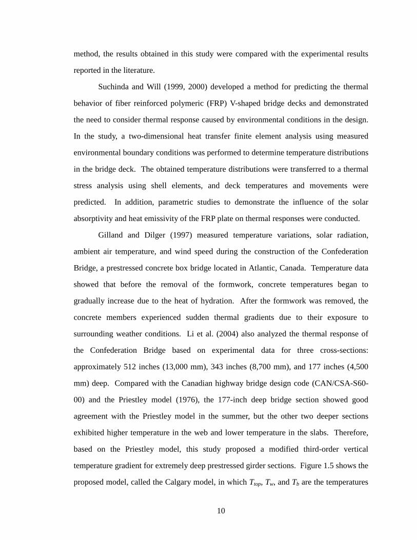
10

method, the results obtained in this study were compared with the experimental results

reported in the literature.

Suchinda and Will (1999, 2000) developed a method for predicting the thermal

behavior of fiber reinforced polymeric (FRP) V-shaped bridge decks and demonstrated

the need to consider thermal response caused by environmental conditions in the design.

In the study, a two-dimensional heat transfer finite element analysis using measured

environmental boundary conditions was performed to determine temperature distributions

in the bridge deck. The obtained temperature distributions were transferred to a thermal

stress analysis using shell elements, and deck temperatures and movements were

predicted. In addition, parametric studies to demonstrate the influence of the solar

absorptivity and heat emissivity of the FRP plate on thermal responses were conducted.

Gilland and Dilger (1997) measured temperature variations, solar radiation,

ambient air temperature, and wind speed during the construction of the Confederation

Bridge, a prestressed concrete box bridge located in Atlantic, Canada. Temperature data

showed that before the removal of the formwork, concrete temperatures began to

gradually increase due to the heat of hydration. After the formwork was removed, the

concrete members experienced sudden thermal gradients due to their exposure to

surrounding weather conditions. Li et al. (2004) also analyzed the thermal response of

the Confederation Bridge based on experimental data for three cross-sections:

approximately 512 inches (13,000 mm), 343 inches (8,700 mm), and 177 inches (4,500

mm) deep. Compared with the Canadian highway bridge design code (CAN/CSA-S60-

00) and the Priestley model (1976), the 177-inch deep bridge section showed good

agreement with the Priestley model in the summer, but the other two deeper sections

exhibited higher temperature in the web and lower temperature in the slabs. Therefore,

based on the Priestley model, this study proposed a modified third-order vertical

temperature gradient for extremely deep prestressed girder sections. Figure 1.5 shows the

proposed model, called the Calgary model, in which Ttop, Tw, and Tb are the temperatures

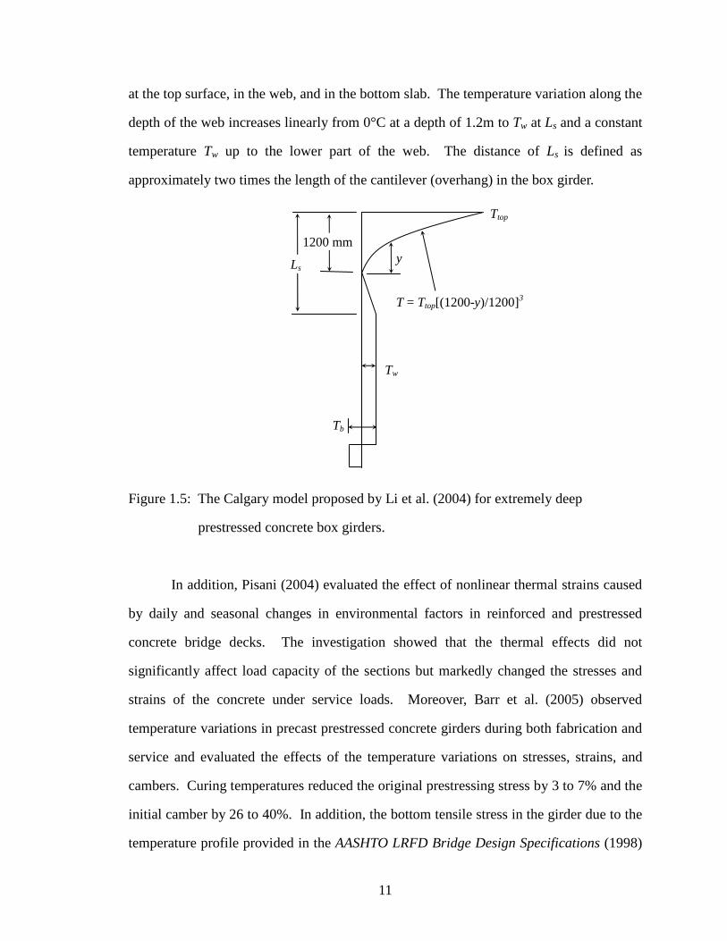
11

at the top surface, in the web, and in the bottom slab. The temperature variation along the

depth of the web increases linearly from 0°C at a depth of 1.2m to Tw at Ls and a constant

temperature Tw up to the lower part of the web. The distance of Ls is defined as

approximately two times the length of the cantilever (overhang) in the box girder.

Figure 1.5: The Calgary model proposed by Li et al. (2004) for extremely deep

prestressed concrete box girders.

In addition, Pisani (2004) evaluated the effect of nonlinear thermal strains caused

by daily and seasonal changes in environmental factors in reinforced and prestressed

concrete bridge decks. The investigation showed that the thermal effects did not

significantly affect load capacity of the sections but markedly changed the stresses and

strains of the concrete under service loads. Moreover, Barr et al. (2005) observed

temperature variations in precast prestressed concrete girders during both fabrication and

service and evaluated the effects of the temperature variations on stresses, strains, and

cambers. Curing temperatures reduced the original prestressing stress by 3 to 7% and the

initial camber by 26 to 40%. In addition, the bottom tensile stress in the girder due to the

temperature profile provided in the AASHTO LRFD Bridge Design Specifications (1998)

y

Ttop

T = Ttop[(1200-y)/1200]3

1200 mm

Tw

Tb

Ls

12

was 370 psi which corresponds to 60% of the allowable concrete tensile stress of 6��,

in which �� is compressive strength of concrete in psi.

The AASHTO bridge specifications were also reviewed for recommendations or

guidelines relevant to the thermal behavior of bridge systems induced by environmental

conditions. Prior to 1989, the America Association of State Highway and Transportation

Officials (AASHTO) provided only uniform temperature changes and did not address

thermal gradients for the design of bridge structures. According to Roberts-Wollman et

al. (2002), bridge engineers who were concerned about the effects of thermal gradients on

concrete bridges generally referred to the Priestley model (Priestley, 1976) as previously

shown in Figure 1.3 or used vertical and transverse temperature differentials, 10°C (18°F)

and 15°C (27°F), respectively, recommended by the Post Tensioning Institute (PTI,

1977). However, the temperatures provided in the PTI manual are not appropriate for

selecting proper temperature differentials in bridge structures.

In 1989, the AASHTO, based on the National Cooperative Highway Research

Program (NCHRP) Report 276, provided uniform bridge temperatures and differential

temperature distributions and published the AASHTO Guide Specifications, Thermal

Effects in Concrete Bridge Superstructures (1989) for the design of reinforced and

prestressed concrete bridge superstructures. The uniform bridge temperatures, which

result in the expansion and contraction of bridge superstructures, were termed “effective

bridge temperatures” in the AASHTO Guide Specifications (1989). The guidelines

provided the values of maximum and minimum effective bridge temperatures based on

maximum and minimum normal air temperatures at the bridge site. Table 1.1 presents

the temperatures correlated with the normal daily air temperatures for concrete bridges.

The profile and values of the vertical temperature differentials from the 1989 AASHTO

Guide Specifications are presented in Figure 1.6. The maximum temperature differences

were defined in terms of four solar radiation zones for the United States as shown in

Figure 1.7.

13

Table 1.1: Correlation between the effective bridge temperatures and normal daily air

temperatures (AASHTO, 1989).

Normal Daily Minimum

Temperature, (°F)

Minimum Effective Bridge Temperature

(°F)

Normal Daily Maximum

Temperature, (°F)

Maximum Effective Bridge Temperature

(°F)

-30 - 3 -25 0 55 66 -20 3 60 69 -15 5 65 73 -10 8 70 77 - 5 11 75 80 0 13 80 84 5 16 85 88 10 19 90 92 15 22 95 95 20 25 100 98 25 29 105 101 30 32 110 105 35 35 40 38

Figure 1.6: Vertical temperature gradient for concrete superstructures (AASHTO, 1989).

Zone T1 (°F) T2 (°F) T3 (°F)

1 54 14 5

2 46 12 4

3 41 11 4

4 38 9 3

T1

T2

T3

5 °F

0.33 ft

0.66 ft

D3

0.66 ft

d

3.28

(or

0.6

6d) ft

14

Figure 1.7: Solar radiation zones for the United States (AASHTO, 1989). Based on the AASHTO Guide Specifications (1989), the AASHTO LRFD Bridge

Design Specifications (2007) simplified the uniform temperatures and vertical

temperature gradients. Section 3.12.2 specifies minimum and maximum temperatures

associated with uniform thermal movements. For concrete deck bridges with concrete

girders, the minimum and maximum temperatures are specified as 10°F and 80°F in a

moderate climate and 0°F and 80°F in a cold climate. From the AASHTO Specifications

(2007), the climate is determined by the number of freezing days, defined as daily

average temperature of less than 32°F. If the total freezing days a year are less than 14

days, the climate is considered to be moderate. In addition, Section 3.12.3 provides the

vertical temperature gradient. Figure 1.8 shows the vertical temperature gradient in

concrete superstructures with concrete decks. The magnitude of the temperature

gradients, T1 and T2, are determined in accordance with solar radiation zones, shown in

15

Figure 1.7. Dimension A in Figure 1.8 is 12.0 inches for concrete superstructures which

are 16.0 inches or more in depth. For concrete sections shallower than 16.0 inches,

Dimension A is the smaller of 4.0 inches and the depth of concrete superstructure.

Temperature value T3 in Figure 1.8 can be taken as 0.0°F unless a site-specific study is

made to determine an appropriate value.

Figure 1.8: Vertical temperature gradient for concrete superstructures (AASHTO, 2007).

1.2.2 Girder Sweep and Support Conditions in Prestressed Concrete Girders

For stability problems associated with girder imperfections and support conditions

in the prestressed concrete bridge girders, few studies have been carried out. Some initial

research were conducted by Laszlo and Imper (1987) and Mast (1989, 1993) for a girder

suspended from lifting devices and for a girder on elastic supports during transportation.

For the girder on elastic supports, they proposed a method to evaluate the girder safety

against overturning. The method, which differed from a traditional stability analysis, was

based on the ratio of a resisting moment at the support to an overturning moment induced

by the girder sweep and support slopes. However, to the author’s knowledge, no specific

Zone T1 (°F) T2 (°F)

1 54 14

2 46 12

3 41 11

4 38 9

T1

T2

4 "

A

8 "

Depth of Superstructure

T3 ≤ 5°F

16

method or guideline that can analyze the lateral stability of the girders placed on elastic

bearing supports during construction has been provided. Consequently, Oesterle et al.

(2007) alternatively used the method proposed by Mast (1989, 1993) for a girder on

elastic supports during transportation and investigated prestressed concrete girders which

collapsed after placing on elastic bearing supports prior to the installation of lateral and

cross bracing in Arizona. According to the investigation conducted by Oesterle et al.

(2007), a number of factors such as initial sweep, thermal sweep, and support slopes

could combine to cause the lateral instability of the girders during construction. The

report recommended that the position of the girder ends and the surfaces of all the

bearings should be carefully checked during the erection of the girders. In addition,

bracing at the both ends of the girders should be added as soon as the girders are erected.

Furthermore, the PCI Bridge Design Manual (2003) was reviewed for guidelines

and recommendations relevant to the support conditions of precast prestressed concrete

bridge girders. Section 3.6 of the PCI Manual describes methods and procedures to

install precast concrete bridge components. Section 3.6.2 emphasizes the establishment

of uniform bearings at the beam ends for the stability of precast flexural concrete

members. For this purpose, this Section indicates that “The support surfaces should be

checked for horizontal and vertical control, as well as flatness and level or slope”. The

flatness of the support is limited to 1/16 inches as a tolerance. Since the beams can also

fall off the support due to forces of natures, including wind, earthquake, or thermally-

induced sweep, Section 3.7 of the PCI Manual which treats temporary diaphragm for

construction indicates that “After the beams have been erected, and before they are

permanently connected into the structure … temporary braces consisting of steel or

timber are used to stabilize the beams”.

In addition, Section 8.3 of the PCI Bridge Design Manual (2003), based on the

studies conducted by Mast (1989, 1993), addresses the lateral stability of slender

members during handling and shipping. For a beam hanging from lifting devices, the

17

rollover of the beam is primarily governed by the properties of the beam while for a beam

supported on flexible supports being transported on a truck, the rollover is significantly

influenced by the conditions of the support and the geometry of the roadway. For the

evaluation of the safety and stability against rollover (or, overturning) failure during

shipping and lifting, Section 8.3 provides explicit calculation procedures and minimum

sweep tolerances in which the initial sweep of the prestressed concrete I-beams is limited

to be 1/8 inches per 10 feet of member length. The PCI Bridge Design Manual (2003),

however, does not provide any specific guidelines and recommendations for the beams in

an erected condition, especially during construction prior to the installation of

diaphragms. Furthermore, according to the PCI Manual, elastomeric bearing pads, used

predominantly as beam supports, can become highly nonlinear when the reaction load is

outside the kern of the bearing pads. Therefore, the nonlinear response of the bearing

pads can result in serious stability problem associated with a beam rollover. In addition,

the PCI Tolerance Manual for Precast and Prestressed Concrete Construction (2000)

was reviewed for the construction tolerance of the bridge girders. Only Section 12.11 of

the PCI Tolerance Manual limits bearing eccentricity which is defined as the difference

between the centerline of the bottom of the beam and the centerline of the elastomeric

bearing pads as shown in Figure 1.9, to ±1 inch.

18

Figure 1.9: The eccentricity of elastomeric bearing pad relative to the centerline of the

bottom of the girder.

The AASHTO bridge design and construction specifications were also reviewed

for the stability of precast prestressed concrete girders related to girder sweep and support

conditions. Section 5.14.1.2.1 of the AASHTO LRFD Bridge Design Specifications

(2007) requires the responsibility of the contractor for the safe shipping and erection, and

Section 5.14.3.3 states the need to consider the potential of the bucking in tall thin web

sections. For the uncertainties of bearing contacts, Section 14.4.2.1 of the specifications

provides a rotation of 0.005 rad. as a tolerance. Moreover, in the AASHTO LRFD Bridge

Construction Specifications (2004), Section 8.13.6 indicates that “the contractor shall be

responsible for the safety of precast members during all stages of construction” and “after

a member has been erected and until it secured to the structure, temporary braces shall be

provided as necessary to resist wind or other loads”. Neither the AASHTO LRFD Bridge

Design Specifications (2007) nor the AASHTO LRFD Bridge Construction Specifications

(2004) provide any specific guidelines related to the stability of precast prestressed

concrete girders during construction.

Bearing Eccentricity

Bridge Girder Elastomeric Bearing Pad

19

1.3 Research Scope and Objectives

The objectives of this research are to investigate variations in the temperature

distributions of precast prestressed concrete bridge girders under various environmental

conditions and to evaluate the global behavior of the bridge girders due to the

combination of these thermal movements, initial imperfections, and support conditions.

For the environmental thermal effects and temperature variations in the

prestressed concrete bridge girders, this research conducted a one-year experiment on a

BT-63 prestressed concrete girder segment to investigate the relationships between

vertical and transverse temperature distributions and environmental conditions. A two-

dimensional transient finite element heat transfer model was developed to predict the

temperature variations and distributions in the bridge girder based on environmental

conditions. For the validation of the proposed heat transfer model, the girder

temperatures obtained from the heat transfer analysis were compared with the

measurements. This study also determined extremes in seasonal environmental

conditions pertaining to the largest vertical and transverse temperature differentials and

proposed vertical and transverse thermal gradients for the design of the prestressed

concrete bridge girders. The effects of seasonal variations and different bridge

orientations on the vertical and transverse temperature differentials are also examined.

Based on these extreme temperature distributions, the thermal response and global

behavior of the prestressed concrete bridge girder at the time of construction (without the

deck or diaphragms) were investigated using a three-dimensional finite element analysis.

This analysis included the effects of initial geometry imperfections and support slopes

combined with thermal movements on the behavior of the bridge girder. To account for

the nonlinear behavior of elastomeric bearing pads used as a support system in precast

prestressed concrete bridge girders, this study also considered the compressive stiffness

of the bearing pads.

20

This research also performed a sensitivity study to determine the effects of

changes in the thermal conductivity, the specific heat, the solar absorptivity, and the

coefficient of thermal expansion of concrete on the temperature distributions and thermal

movements.

1.4 Overview and Structure of the Thesis

Chapter 2 describes an experimental investigation into environmental thermal

effects and temperature variations over the section of a BT-63 girder and investigates

variations in vertical and transverse temperature differentials and the corresponding

environmental conditions from the measurements taken from April 2009 to March 2010.

Using the measured environmental boundary conditions, Chapter 3 presents a two-

dimensional finite element heat transfer model which accounts for heat convection, heat

conduction, heat irradiation, and heat radiation. In the numerical analysis, the intensity of

solar radiation incident on each surface of the girder is estimated considering the location

and orientation of the bridge, the geometry and shadow of the girder, the position of the

sun, and the solar radiation measured on a horizontal surface. The temperature variations

and distributions obtained from the heat transfer analysis are compared with those

obtained from the measurements for validation. In Chapter 4, the temperature fields

defined from the heat transfer analysis are transferred to a three-dimensional finite

element model, and the thermal stress analysis is then performed to determine the thermal

response of the BT-63 girder. The prestressing forces are modeled as initial stress

conditions and the support conditions as simply-supported boundary conditions.

Chapter 5 determines extremes in seasonal environmental conditions pertaining to

the maximum vertical and transverse temperature distributions. Based on the extreme

environmental conditions, the two-dimensional heat transfer model is employed to

evaluate the effects of seasonal variations and different bridge orientations on the

temperature distributions in four AASHTO-PCI standard sections. As a result, this

21

chapter proposes revised vertical and new transverse thermal gradients applicable to the

design of concrete and prestressed concrete bridge girders in the United States. Chapter 6

uses three-dimensional thermal stress analysis to determine thermal response induced by

the maximum temperature distributions. In addition to the thermal movements, this

chapter evaluates the effects of initial geometry imperfections and bearing slopes on the

global behavior of a prestressed concrete bridge girder during construction. The

nonlinear behavior of elastomeric bearing pads is idealized by nonlinear springs with the

effective compressive stiffness of the bearing pad. Furthermore, this study proposes a

simple beam model that can calculate thermal movements induced by nonlinear

temperature distributions.

Chapter 7 discusses the influence of thermal properties of concrete on temperature

distributions and thermal movements in prestressed concrete bridge girders. The

parameters associated with the temperature distributions are thermal conductivity,

specific heat, and solar absorptivity. For the thermal movements, the influence of the

coefficient of thermal expansion is evaluated using the three-dimensional thermal stress

analysis. Finally, Chapter 8 summarizes the results of the current study and recommends

future studies for the thermal responses and global behavior of concrete and prestressed

concrete bridges.

22

CHAPTER 2

EXPERIMENTAL INVESTIGATION OF THERMAL EFFECTS

2.1 Introduction

This study carries out an experimental investigation to determine the temperature

distributions in a prestressed concrete bridge girder due to solar radiation, ambient air

temperature, and wind speed. Since prestressed concrete girders have commonly been

designed using AASHTO-PCI sections (PCI, 2003), this study chose an AASHTO BT-63

for the cross-section of a test girder. The length of the test girder was designed to be five

feet since temperature distributions were assumed to be constant in the longitudinal

direction. The experiment was conducted during the months of April 2009 to March

2010 in the east-west direction so that only the top surface and one side of the girder

received direct solar radiation from the sun. This orientation would provide the girder

with extremes in transverse temperature distributions.

2.2 Specimen Preparation

The five-foot long test bridge girder was cast at a precasting plant of Standard

Concrete Products in Atlanta, Georgia on October 27, 2008. Prestressing forces were

produced by a total of twelve low relaxation strands, 0.5 inches in diameter. Four strands

were set in the top flange, and the other eight strands were distributed in a layer of the

bottom flange as shown in Figure 2.1. These strands were prestressed to 10,700 pounds

per strand in the top flange and to 35,000 pounds per strand in the bottom flange. As a

result, the total jacking force on the test girder was 322,800 pounds. Three days after the

concrete pouring, the tension forces of the strands were released and the steel molds were

removed from the five-foot girder on October 29, 2008. At 28 days, the compressive

strength tests were performed on three 6-inch and 12-inch cylinder specimens, resulting

in an average compressive strength of 9.0 ksi.

23

Figure 2.1: The cross-section of the BT-63 specimen and the layout of the prestressing strands.

On November 14, 2008, the five-foot girder was moved to the Structures

Laboratory at Georgia Institute of Technology. Both ends of the girder were insulated by

extruded polystyrene sheets to minimize heat transfer between the end of the girder and

the air. The pickup steel exposed to the air was wrapped with polyethylene pipe

insulation to minimize heat transfer between the steel and the air. The specimen was then

moved to the parking lot of the Structures Laboratory and placed in an area

approximately 75 feet away from the main building since the shadow of the main

building was calculated to be a maximum 74 feet long in December. Moreover, to reduce

heat radiation from the ground to the bottom of the girder, steel blocks were used to raise

the girder approximately 1.5 feet above the ground. A wooden board was also placed

between the specimen and the steel block to minimize heat transfer between the steel

block and the concrete. In addition, a dark foam sheet was placed on the ground

underneath the girder to minimize the heat reflection and radiation from the ground. Data

acquisition systems collecting the measurements were installed next to the specimen.

Figure 2.2 illustrates the specimen set-up in the parking lot of the Structures Laboratory.

Prestressing strands 63" 45"

4.5"

6"

4"

3.5"

3'-6"

24

Figure 2.2: The specimen set-up in the parking lot of the Structures Laboratory.

2.3 Instrumentation

The primary environmental factors affecting the temperature variation in bridges

are solar radiation, ambient air temperature, and wind speed. The intensity of solar

radiation incident on the surfaces of the girder was measured on the horizontal and

vertical surfaces of the top flange of the test girder. Ambient air temperature and wind

speed were recorded approximately one foot above the top surface of the girder. A total

of twenty-eight thermocouples were used to measure the internal and external

temperatures of the girder. Eleven thermocouples were placed inside the girder and

seventeen thermocouples on the outside surface.

Data Acquisition Systems

Insulated Pickup Steel

Steel Block

Wooden Board

Foam Sheet

Insulated End

Insulated End

25

2.3.1 Environmental Variables

Two SP-110 pyranometers manufactured by Apogee Instruments were used to

measure the intensity of solar radiation incident on a horizontal and vertical surface of the

girder. One pyranometer was installed on the top surface of the top flange to measure

solar radiation on a horizontal surface, and another was installed on the side of the top

flange to measure vertical solar radiation. Figure 2.3 shows the two pyranometers on the

surfaces of the top flange in the girder.

Figure 2.3: Pyranometers installed at the top flange of the test girder.

One Type-K bare lead thermocouple was installed to measure ambient air

temperature approximately one foot above the corner of the top surface. The

thermocouple was covered by plywood to avoid contact with water on a rainy day and to

minimize the influence of direct solar radiation during the day. The wind speed was

measured with a three-cup anemometer, 03001 Wind Sentry Set manufactured by

Campbell Scientific. The anemometer was also installed approximately one foot above

the top surface on the other side of the girder. Figure 2.4 shows the thermocouple used to

measure ambient air temperature and the anemometer installed on the top surface of the

girder.

Pyranometers

26

(a) Thermocouple for ambient air temperature (b) Anemometer for wind speed Figure 2.4: Thermocouple and anemometer installed on the top surface of the test girder.

2.3.2 Girder Temperatures

For the investigation of the temperature variations of the girder in the vertical and

lateral directions, a total of 28 Type-K thermocouples were installed at mid-span. Figure

2.5 shows the specific locations of all the internal and external thermocouples. Internal

temperatures were measured using eleven Type-K bare lead thermocouples, and surface

temperatures were measured using seventeen Type-K washer thermocouples with PFA

insulation. As shown in Figure 2.6, the eleven internal thermocouples were placed inside

the girder at mid-span prior to the concrete pour. Figure 2.7 shows the seventeen external

thermocouples installed on the BT-63 girder at mid-span.

27

(a) Thermocouple locations (b) Thermocouple numbers

Figure 2.5: The locations of thermocouples installed at mid-span.

Figure 2.6: Internal thermocouples installed at mid-span.

(b) In the top flange

(c) In the bottom flange (a) In the web

6"

20.5"

2"

20.5"

2"

6" 7"

8" 9" 4"

3"

26 28 27

25 24

22

20

18

21

23

19

14 15

12 13

16 17

10 9 11

8

7

6

5 3 4 1 2

28

Figure 2.7: External thermocouples installed at mid-span.

2.3.3 Data Acquisition Systems

To collect data measured in the experiment automatically, this study employed

two data acquisition systems: an SCXI-1000 chassis and a USB-6008 device. First, this

experiment used the National Instruments SCXI-1000 chassis, which holds an SCXI-

1102 module and an SCXI-1303 terminal block, to measure girder temperatures, ambient

air temperature, and solar radiation. The measurements were controlled through a

National Instruments DAQCard Al-16E-4 with a PSHR68-68M I/O cable using a

sampling rate of 100 Hertz every five minutes. This experiment also used the National

Instruments USB-6008 device to measure wind speed in AC volts at a sampling rate of

1,000 Hertz at the same interval of five minutes since the rotation of the cup wheel

produces an AC sine wave with a frequency proportional to the wind speed. Figure 2.8

illustrates the configuration of the two data acquisition systems in detail.

(b) On the top surface of the top flange

(a) On the surfaces of the web and bottom flanges

29

Figure 2.8: The configuration of data acquisition systems for the measurements.

2.4 Measurements of Environmental Conditions and Girder Temperatures

This section presents the results of solar radiation, ambient air temperature, and

wind speed taken from April 2009 to March 2010. Internal and external girder

temperatures were also measured simultaneously with the environmental factors.

2.4.1 Environmental Conditions

From the measurements taken from April 2009 to March 2010, this study assessed

variations in daily environmental conditions, solar radiation, ambient air temperature, and

wind speed. Table 2.1 summarizes the daily solar radiation, daily maximum and

minimum air temperatures, and daily average wind speed calculated from the

measurements for selected sunny days, on which large vertical and/or transverse

temperature distributions were measured.

SCXI-1303 SCXI-1102 SCXI-1000

USB-6008

Desktop

DAQCard Al-16E-4 PSHR68-68M I/O

30

Table 2.1: The daily environmental conditions for selected sunny days during the

measurements from April 2009 to March 2010.

Dates

Daily Solar Radiation (MJ/m2)

Daily Air Temperature (°C)

Daily Wind speed, (m/sec)

Horizontal Vertical Maximum Minimum Variance Average Maximum

4/24/2009 27.0 10.9 32.1 13.6 18.5 0.6 3.1

5/20 27.5 8.8 25.8 15.6 10.2 1.3 5.3

5/30 29.5 7.7 30.4 15.6 14.8 0.5 2.5

6/ 1 28.8 7.4 33.3 18.8 14.5 0.4 2.8

6/23 26.4 7.2 34.4 24.1 10.3 0.5 7.0

7/18 28.8 7.5 29.3 18.3 11.0 0.8 5.1

8/25 22.0 10.0 32.3 21.4 10.9 0.6 3.0

9/30 21.0 16.8 24.6 10.0 14.6 0.4 2.8

10/ 1 20.6 16.4 26.1 10.8 15.3 0.4 2.5

10/20 18.0 17.8 20.8 4.2 16.6 0.2 1.9

11/ 8 13.8 14.3 23.9 7.3 16.6 0.2 1.9

11/15 14.7 19.0 23.3 8.6 14.7 0.3 2.4

11/20 13.6 18.0 18.7 4.2 14.5 0.2 2.4

12/22 11.1 17.8 15.1 0.2 14.9 0.4 2.6

1/13/2010 12.8 20.7 7.8 -5.1 12.9 0.2 1.8

2/ 8 13.6 15.6 9.8 -1.2 11.0 0.6 3.5

2/19 15.8 16.5 12.4 2.5 9.9 0.4 2.3

2/28 18.6 18.6 10.3 1.0 9.3 0.9 2.9

3/ 5 20.4 18.6 10.5 1.2 9.3 0.5 3.2

3/23 19.4 13.0 17.9 3.2 14.7 1.0 5.3

31

Solar Radiation

Figure 2.9 illustrates variations in the daily solar radiation on the horizontal and

vertical surfaces during the months of April 2009 to March 2009. The gaps in the data

were due to system repair and maintenance. The daily horizontal and vertical solar

radiation shown in Figure 2.9 were calculated by using the trapezoid method to integrate

the radiation data measured on the horizontal and vertical surfaces. With seasonal

changes in the intensity of solar radiation on the horizontal and vertical surfaces, the

highest solar radiation on the horizontal surface was recorded in the summer during the

months of June, July, and August, and the highest solar radiation on the vertical surface

was recorded in the late fall and winter during the months of November, December, and

January.

Figure 2.10 shows variations in solar radiation on the horizontal and vertical

surfaces for June 1, October 1, and November 15, 2009. June 1 and November 15

exhibited the largest vertical and transverse temperature distributions during the

measurements. October 1 was selected to evaluate the transition of the environmental

conditions from the summer to the late fall. Table 2.2 summarizes daily solar radiation

calculated from the measurements. From June 1 to November 15, 2009, the daily

horizontal solar radiation reduced from 28.8 to 14.7 MJ/m2 while the daily vertical solar

radiation increased from 7.4 to 20.9 MJ/m2. Similarly, the intensity of solar radiation on

the horizontal surface was the highest on June 1, and the solar radiation on the vertical

surface was the highest on November 15.

Table 2.2: Solar radiation measured on the horizontal and vertical surfaces on June 1,

October 1, and November 15, 2009.

Dates Daily Solar Radiation (MJ/m2) Maximum Solar Radiation (W/m2)

Horizontal Vertical Horizontal Vertical

June 1 28.8 7.4 1,052 302

October 1 20.8 16.7 862 672

November 15 14.7 20.9 674 867

32

(a) Daily solar radiation on the horizontal surface

(b) Daily solar radiation on the vertical surface

Figure 2.9: Variation in daily solar radiation on horizontal and vertical surfaces during

the months of April 2009 to March 2010.

4/16 6/1 7/1 8/1 9/1 10/1 11/1 12/1 1/1 2/1 3/10

5

10

15

20

25

30

35

Dai

ly s

olar

rad

iatio

n (M

J/m

2 )

5/1 6/1 7/1 8/1 9/1 10/1 11/1 12/1 1/1 2/1 3/10

5

10

15

20

25

30

35

Dai

ly s

olar

rad

iatio

n (M

J/m

2 )

33

(a) June 1 (b) October 1 (c) November 15

Figure 2.10: Solar radiation measured on the horizontal and vertical surfaces on June 1,


Air Temperature

The maximum and minimum measured ambient air temperatures from April 2009

to March 2010 are shown in Figure 2.11. As expected, the daily maximum and minimum

air temperatures increased in the summer and decreased from the summer to the winter.

For the three days, June 1, October 1, and November 15, Figure 2.12 shows variations in

the ambient air temperatures as a function of the time of day, in which minimum

temperatures were measured around sunrise, and maximum temperatures were measured

around 2 or 3 p.m.

6 8 10 12 14 16 18 200

200

400

600

800

1000

12001052

(12:43)

302(13:08)

Time (hr)

Sol

ar r

adia

tion

(W/m

2 )

Horizonal surfaceVertical surface

6 8 10 12 14 16 18 20

862(12:14)

672(13:14)

Time (hr)


6 8 10 12 14 16 18 20

674(12:09)

867(12:24)

Time (hr)


34

Figure 2.11: Variation in daily maximum and minimum air temperatures during the

months of April 2009 to March 2010.

Figure 2.12: Ambient air temperatures measured on June 1, October 1, and November

15, 2009.

5/1 6/1 7/1 8/1 9/1 10/1 11/1 12/1 1/1 2/1 3/1

0

10

20

30

40T

empe

ratu

re (o C

)

Daily maximum

Daily minimum

32

50

68

86

104

Tem

pera

ture

(o F)

2 4 6 8 10 12 14 16 18 20 220

10

20

30

40

18oC(05:33)

34oC(15:07)

Time (hr)

Tem

pera

ture

(o C

)

11oC(05:39)

24oC(14:19)

9oC(07:19)

23oC(15:04)

June 1October 1November 15

0

50

68

86

104

Tem

pera

ture

(o F

)

35

Wind Speed

This study also evaluated variations in daily average wind speed which was

calculated by integrating the measurements using the trapezoid numerical method and

dividing the integration by the total measurement time of the day. The daily average

wind speed shown in Figure 2.13 is less than 3 m/sec, or 6.7 mph during the

measurements taken from April 2009 to March 2010, even though somewhat higher

values occurred in the winter. The record maximum wind speed, or the highest wind

speed during the measurements, was 14.9 m/sec, or 33.2 mph, on June 8, 2009. In

addition, Figure 2.14 shows the wind speed less than 1 m/sec, or 2.2 mph, for June 1,

October 1, and November 15.

Figure 2.13: Variation in daily average wind speed during the months of April 2009 to

March 2010.

5/1 6/1 7/1 8/1 9/1 10/1 11/1 12/1 1/1 2/1 3/10

1

2

3

Ave

rage

win

d sp

eed

(m/s

ec)

0

2.2

4.5

6.7

Ave

rage

win

d sp

eed

(mph

)

36

Figure 2.14: Wind speed measured on June 1, October 1, and November 15, 2009.

2.4.2 Girder Temperatures

In addition to variations in daily environmental conditions, Figures 2.15 to 2.19

illustrate variations in daily highest and lowest girder temperatures measured in the top

flange, the web, and the bottom flange during the months of April 2009 to March 2010.

As mentioned earlier, the readings contain several gaps due to system repair and

maintenance.

For the top flange, Figures 2.15 and 2.16 show the daily highest and lowest

temperature changes on the south side (thermocouple 2) and on the top surface

(thermocouple 28) during the measurements, respectively. With high solar radiation and

high air temperature in the summer, the temperatures of the top flange were the

maximum in the summer and decreased with seasonal changes from the summer to the

winter.

2 4 6 8 10 12 14 16 18 20 220

1

2

3

0

2.2

4.5

6.7

2 4 6 8 10 12 14 16 18 20 220

1

2

3

Win

d sp

eed

(m/s

ec)

0

2.2

4.5

6.7

Win

d sp

eed

(mph

)

2 4 6 8 10 12 14 16 18 20 220

1

2

3

Time (hr)

0

2.2

4.5

6.7

June 1

October 1

November 15

37

Variations in the daily highest and lowest temperatures in the middle of the girder

web (thermocouple 7) are presented in Figure 2.17, which indicates as expected that the

maximum temperature was recorded in the summer, and the minimum temperature was

recorded in the winter. In addition, Figures 2.18 and 2.19 show variations in the daily

highest and lowest temperatures on the south vertical surface (thermocouple 14) and on

the bottom surface of the bottom flange (thermocouple 13), respectively.

38

(a) Daily highest temperature

(b) Daily lowest temperature

Figure 2.15: Variation in the daily highest and lowest temperatures in the south side of

the top flange (thermocouple 2) during the months of April 2009 to March

2010.

5/1 6/1 7/1 8/1 9/1 10/1 11/1 12/1 1/1 2/1 3/1-10

0

10

20

30

40

50

60

Tem

pera

ture

(o C)

14

32

50

68

86

104

122

140

Tem

pera

ture

(o F)

5/1 6/1 7/1 8/1 9/1 10/1 11/1 12/1 1/1 2/1 3/1-10

0

10

20

30

40

50

60

Tem

pera

ture

(o C)

14

32

50

68

86

104

122

140

Tem

pera

ture

(o F)

2

2

39



Figure 2.16: Variation in the daily highest and lowest temperatures on the top surface of

the girder (thermocouple 28) during the months of April 2009 to March

2010.

5/1 6/1 7/1 8/1 9/1 10/1 11/1 12/1 1/1 2/1 3/1-10

0

10

20

30

40

50

60

Tem

pera

ture

(o C)

14

32

50

68

86

104

122

140

Tem

pera

ture

(o F)

5/1 6/1 7/1 8/1 9/1 10/1 11/1 12/1 1/1 2/1 3/1-10

0

10

20

30

40

50

60

Tem

pera

ture

(o C)

14

32

50

68

86

104

122

140

Tem

pera

ture

(o F)

28

28

40



Figure 2.17: Variation in the daily highest and lowest temperatures in the middle of the

girder web (thermocouple 7) during the months of April 2009 to March

2010.

4/16 5/1 6/1 7/1 8/1 9/1 10/1 11/1 12/1 1/1 2/1 3/1 3/31-10

0

10

20

30

40

50

Tem

pera

ture

(o C)

14

32

50

68

86

104

122

Tem

pera

ture

(o F)

5/1 6/1 7/1 8/1 9/1 10/1 11/1 12/1 1/1 2/1 3/1-10

0

10

20

30

40

50

Tem

pera

ture

(o C)

14

32

50

68

86

104

122

Tem

pera

ture

(o F)

7

7

41



Figure 2.18: Variation in the daily highest and lowest temperatures on the south vertical

surface of the bottom flange (thermocouple 14) during the months of April

2009 to March 2010.

5/1 6/1 7/1 8/1 9/1 10/1 11/1 12/1 1/1 2/1 3/1-10

0

10

20

30

40

50

Tem

pera

ture

(o C)

14

32

50

68

86

104

122

Tem

pera

ture

(o F)

5/1 6/1 7/1 8/1 9/1 10/1 11/1 12/1 1/1 2/1 3/1-10

0

10

20

30

40

50

Tem

pera

ture

(o C)

14

32

50

68

86

104

122

Tem

pera

ture

(o F)

14

14

42



Figure 2.19: Variation in the daily highest and lowest temperatures on the bottom surface

of the girder (thermocouple 13) during the months of April 2009 to March

2010.

5/1 6/1 7/1 8/1 9/1 10/1 11/1 12/1 1/1 2/1 3/1-10

0

10

20

30

40

50

Tem

pera

ture

(o C)

14

32

50

68

86

104

122

Tem

pera

ture

(o F)

5/1 6/1 7/1 8/1 9/1 10/1 11/1 12/1 1/1 2/1 3/1-10

0

10

20

30

40

50

Tem

pera

ture

(o C)

14

32

50

68

86

104

122

Tem

pera

ture

(o F)

13

13

43

2.5 Variations in Vertical and Transverse Temperature Differences

Based on the measurements, the vertical temperature differences were determined

from the difference of the highest and lowest temperatures along the depth of the girder

(thermocouples 28, 5, 6, 7, 8, 9, 12, 13), and the transverse temperature differences were

determined from the temperature differences across the top flange (thermocouples 2, 4, 5,

3, 1), the girder web (thermocouples 20, 7, 21), and the bottom flange (thermocouples 14,

10, 9, 11, 15).

2.5.1 Vertical Temperature Differences

The highest temperature in the BT-63 section was measured on the top surface

while the lowest temperature was measured in the bottom flange. Figure 2.20 shows a

variation in the daily vertical temperature changes along the depth of the girder

(thermocouples 28, 5, 6, 7, 8, 9, 12, 13) during the measurements. The two largest

vertical temperature differences, 20.9°C (37.6°F) and 20.4°C (36.7°F), were measured on

May 30 and June 1, 2009, respectively. Along with the daily highest temperatures on the

top surface shown in Figure 2.16(a), Table 2.3 summarizes the daily vertical temperature

differences for selected sunny days during the measurements from April 2009 to March

2010. In the summer during the months of May to July, the highest daily girder

temperatures ranged from 46°C (115°F) to 54°C (129°F) and the daily vertical

temperature differences from 18°C (32°F) to 21°C (38°F). With seasonal changes from

the summer to the winter, the highest girder temperatures decreased approximately to

13°C (55°F), and the vertical temperature differences decreased to 9°C (16°F).

44

Figure 2.20: Variation in the daily vertical temperature differences along the depth of the

girder during the months of April 2009 to March 2010.

5/1 6/1 7/1 8/1 9/1 10/1 11/1 12/1 1/1 2/1 3/10

5

10

15

20

25

Tem

pera

ture

(o C)

0

9

18

27

36

45

Tem

pera

ture

(o F)

5/30: 20.9°C (37.6°F)

6/1: 20.4°C (36.7°F)

28

12 13

6

7

8

5

9

45

Table 2.3: The highest daily girder temperatures and the daily vertical temperature

differences for selected sunny days during the months of April 2009 to March

2010.

Dates Highest Girder Temperatures,

°C (°F) Vertical Temperature Differences,

°C (°F)

4/24/2009 45.5 (113.9) 16.7 (30.1)

5/20 41.6 (106.9) 18.0 (32.3)

5/30 49.4 (121.0) 20.9 (37.6)

6/ 1 52.8 (127.1) 20.4 (36.7)

6/23 53.6 (128.5) 18.5 (33.3)

7/18 45.5 (113.8) 18.3 (33.0)

8/25 44.0 (111.2) 15.9 (28.6)

9/30 35.3 (95.6) 13.6 (24.4)

10/ 1 38.4 (101.2) 14.1 (25.3)

10/20 30.9 (87.5) 13.8 (24.9)

11/ 8 32.8 (91.0) 12.5 (22.4)

11/15 30.9 (87.6) 10.9 (19.5)

11/20 26.7 (80.1) 11.1 (19.9)

12/22 20.8 (69.5) 9.4 (16.9)

1/13/2010 13.3 (55.9) 8.7 (15.7)

1/27 15.1 (59.2) 9.1 (16.4)

2/ 8 17.1 (62.8) 8.9 (16.1)

2/19 19.8 (67.7) 10.1 (18.1)

2/28 21.6 (70.8) 11.1 (20.0)

3/ 5 20.4 (68.8) 11.0 (19.8)

3/23 26.9 (80.3) 11.9 (21.4)

46

2.5.2 Transverse Temperature Differences

In addition to the vertical temperature differences, the transverse temperature

differences were determined from the differences between the highest and lowest

temperatures in the top flange, the web, and the bottom flange of the girder. Since the

specimen was oriented in an east-west direction, the highest temperatures were recorded

on the south-facing surfaces, and the lowest temperatures were on the north-facing

surfaces in the web. In the top and bottom flanges, the lowest temperatures were

recorded in the middle of the top and bottom flanges.

Figure 2.21 shows the daily transverse temperature changes across the top flange

(thermocouples 2, 4, 5, 3, 1). The large transverse temperature differences of 10.6°C

(19.1°F) and 10.0°C (18.0°F) were measured on November 8 and 15, 2009, respectively.

For the web, Figures 2.22 to 2.24 illustrate the daily transverse temperature changes

across the top (thermocouples 22, 6, 23), the middle (thermocouples 20, 7, 21), and

bottom (thermocouples 18, 8, 19) of the web, respectively. The transverse temperature

difference in the top of the web shown in Figure 2.22 is around 3°C (5.5°F) with no

specific variations during the year because of the shadow of the top flange. However, the

middle and bottom of the web, which did not have shadow from the top flange in the fall,

spring, and winter seasons, exhibited increases in transverse temperature differences as

shown in Figures 2.23 and 2.24. The large transverse temperature difference in the

middle of the web is 11.4°C (20.4°F) on November 8 and 11.5°C (20.6°F) on November

15, 2009. Similarly, the bottom of the web showed a large transverse temperature

difference of 10.6°C (19.2°F) on October 20 and 9.3°C (16.8°F) on November 15, 2009.

In addition, Figure 2.25 shows the variation in the daily transverse temperature

differences across the bottom flange (thermocouples 14, 10, 9, 11, 15), in which large

differences of 21.5°C (38.7°F) and 20.5°C (36.8°F) were measured on October 1 and

November 15, 2009, respectively.

47

Table 2.4 summarizes the large transverse temperature differences in the top

flange, the web, and the bottom flange for selected sunny days during the measurements

from April 2009 to March 2010. Contrary to the vertical temperature changes, large

transverse temperature differences, approximately 10°C (18°F) in the top flange and the

web and 20°C (38°F) in the bottom flange, were measured in the late fall and winter

during the months of October, November, and December due to high solar radiation on

the vertical surface.

Figure 2.21: Variation in the daily transverse temperature differences in the top flange

during the months of April 2009 to March 2010.

5/1 6/1 7/1 8/1 9/1 10/1 11/1 12/1 1/1 2/1 3/10

5

10

15

20

25

Tem

pera

ture

(o C)

0

9

18

27

36

45

Tem

pera

ture

(o F)

11/8: 10.6°C (19.1°F)

11/15: 10.0°C (18.0°F)

5 2 1 4 3

48

Figure 2.22: Variation in the daily transverse temperature differences in the top of the

web during the months of April 2009 to March 2010.

Figure 2.23: Variation in the daily transverse temperature differences in the middle of the


4/16 5/1 6/1 7/1 8/1 9/1 10/1 11/1 12/1 1/1 2/1 3/10

9

18

27

36

45

Tem

pera

ture

(o C)

0

5

10

15

20

25

Tem

pera

ture

(o F)

5/1 6/1 7/1 8/1 9/1 10/1 11/1 12/1 1/1 2/1 3/10

5

10

15

20

25

Tem

pera

ture

(o C)

0

9

18

27

36

45

Tem

pera

ture

(o F)

11/15: 11.5°C (20.6°F)

11/8: 11.4°C (20.4°F)

22 23

6

22 23

6

20 21

7

49

Figure 2.24: Variation in the daily transverse temperature differences in the bottom of the


Figure 2.25: Variation in the daily transverse temperature differences in the bottom

flange during the months of April 2009 to March 2010.

4/16 5/1 6/1 7/1 8/1 9/1 10/1 11/1 12/1 1/1 2/1 3/10

5

10

15

20

25

Tem

pera

ture

(o C)

0

9

18

27

36

45

Tem

pera

ture

(o F)

5/1 6/1 7/1 8/1 9/1 10/1 11/1 12/1 1/1 2/1 3/10

5

10

15

20

25

Tem

pera

ture

(o C)

0

9

18

27

36

45

Tem

pera

ture

(o F)

10/1: 21.5°C (38.7°F)

11/15: 20.5°C (36.8°F)

10/20: 10.6°C (19.2°F)

11/15: 9.3°C (16.8°F)

18 19

8

914 15

10 11

50

Table 2.4: The daily transverse temperature differences in the top flange, the web, and

the bottom flange for selected sunny days during the months of April 2009 to

March 2010.

Dates Transverse Temperature Differences, °C (°F)

Top flange Top-web Mid-web Bottom-web Bottom flange

4/24/2009 8.3 (14.9) 3.7 (6.7) 3.0 (5.4) 6.7 (12.0) 17.8 (32.0)

5/20 5.3 (9.6) 2.6 (4.6) 2.8 (5.0) 3.0 (5.3) 11.8 (21.2)

5/30 7.6 (13.8) 3.0 (5.4) 2.2 (3.9) 3.4 (6.1) 13.8 (24.8)

6/ 1 7.4 (13.3) 2.8 (5.1) 2.1 (3.7) 3.1 (5.5) 13.8 (24.8)

6/23 7.0 (12.6) 2.6 (4.6) 2.1 (3.8) 2.7 (4.8) 11.9 (21.4)

7/18 6.7 (12.1) 2.5 (4.5) 1.8 (3.2) 3.0 (5.3) 13.7 (24.7)

8/25 6.7 (12.0) 2.8 (5.0) 2.3 (4.1) 7.2 (13.0) 15.9 (28.6)

9/30 8.5 (15.2) 2.9 (5.2) 8.4 (15.2) 9.8 (17.7) 20.6 (37.1)

10/ 1 8.2 (14.8) 2.6 (4.7) 8.9 (16.1) 10.4 (18.6) 21.5 (38.7)

10/20 9.5 (17.1) 3.3 (5.9) 9.9 (17.9) 10.6 (19.2) 16.7 (30.0)

11/ 8 10.6 (19.1) 3.4 (6.0) 11.4 (20.4) 10.3 (18.6) 19.7 (35.4)

11/15 10.0 (18.0) 3.2 (5.8) 11.5 (20.6) 9.3 (16.8) 20.5 (36.8)

11/20 10.5 (19.0) 3.4 (6.2) 11.3 (20.3) 9.6 (17.2) 20.3 (36.5)

12/22 9.8 (17.7) 2.8 (5.1) 9.7 (17.4) 9.4 (17.0) 19.2 (34.6)

1/13/2010 9.8 (17.7) 2.4 (4.2) 8.9 (16.0) 8.8 (15.8) 18.6 (33.5)

1/27 7.3 (13.2) 2.6 (4.7) 8.3 (15.0) 6.9 (12.4) 16.4 (29.5)

2/ 8 7.3 (13.2) 2.6 (4.7) 6.8 (12.3) 6.4 (11.4) 13.5 (24.2)

2/19 7.8 (14.0) 2.9 (5.1) 7.3 (13.1) 8.0 (14.4) 14.5 (26.1)

2/28 7.3 (13.1) 2.6 (4.6) 8.4 (15.1) 9.3 (16.8) 18.0 (32.3)

3/ 5 7.3 (13.1) 3.1 (5.5) 7.5 (13.5) 8.5 (15.2) 17.2 (31.0)

3/23 6.8 (12.2) 3.0 (5.4) 3.2 (5.8) 7.5 (13.4) 17.1 (30.7)

51

2.6 Variations in Vertical and Transverse Temperature Distributions and Gradients

According to the daily vertical and transverse temperature differences in the

girder during the year, the largest vertical temperature difference was recorded in the

summer, and it decreased from the summer to the winter. On the other hand, the largest

transverse temperature differences occurred in the late fall and the winter and the smallest

in the summer. Thus, based on the largest vertical and transverse temperature differences,

June 1 and November 15, 2009 were selected as representative days of the largest vertical

and transverse temperature distributions, respectively. October 1, which showed large

vertical and transverse temperature differences in the fall, was chosen to evaluate the

transition of the largest vertical and transverse temperature distributions from the summer

to the fall.

2.6.1 Vertical Temperature Distributions and Gradients

Figure 2.26 shows vertical temperature distributions through the depth of the BT-

63 section for the three days of June 1, October 1, and November 15, 2009. As noted

previously, the temperature magnitude was the highest on June 1 and the smallest on

November 15. The highest temperature was measured on the top surface of the top

flange (thermocouple 28) and the lowest temperature in the bottom flange (thermocouple

9). In particular, on October 1 and November 15, the temperatures in the girder web

exhibited relatively higher increases due to high solar radiation on the vertical surface.

Thus, the temperature distribution in the web increased with changes from the summer to

the fall. In addition, Figure 2.26 includes temperature distributions, defined by a

minimum average temperature of the girder, which would provide the girder with a

minimum and a constant temperature distribution over the cross-section. The

temperature distributions obtained by the minimum average temperatures shown in

Figure 2.26 were nearly constant at around 24°C (74°F) at 6:33 a.m. on June 1 and 15°C

(59°F) at 7:05 a.m. on October 1 and 13°C (55°F) at 7:40 a.m. on November 15.

52

The vertical temperature gradients, defined by subtracting the minimum

temperature from the vertical temperature distribution, are presented in Figure 2.27. The

representative day of the summer, or June 1, shows a rapid gradient decrease from the top

surface and no large gradient in the web. For October 1 and November 15, which show

lower temperatures on the top surface, the web temperature gradients increased due to an

increase in solar radiation on the vertical surface from the summer to the fall. The

vertical temperature differentials, or the temperature difference between the highest and

lowest temperatures along the depth of the girder, are 20.4°C (36.7°F) on June 1, 14.1°C

(25.3°F) on October 1, and 10.9°C (19.5°F) on November 15, 2009.

53

Thermocouple No. 28 5 6 7 8 9 12 13

Temperature, °C (°F)

on June 1

6:33 a.m. 20.6

(69.1) 23.0

(73.4) 23.9

(75.0) 23.3

(74.0) 23.8

(74.8) 27.1

(80.7) 23.2

(73.7) 23.2

(73.7)

1:42 p.m. 50.9

(123.7) 43.8

(110.8) 34.8

(94.6) 32.8

(91.1) 30.8

(87.5) 30.6

(87.0) 39.7

(103.5) 33.8

(92.8)


on Oct. 1

7:05 a.m. 12.2

(53.9) 14.0

(57.2) 15.4

(59.7) 15.4

(59.7) 16.2

(61.2) 16.4a (61.5)

15.6 (60.1)

15.6 (60.1)

1:15 p.m. 34.1

(93.4) 28.8

(83.9) 21.4

(70.5) 25.9

(78.6) 24.7

(76.5) 21.0 a (69.8)

31.7 (89.0)

21.6 (70.9)


on Nov. 15

7:40 a.m. 9.9

(49.8) 11.6

(52.9) 12.9

(55.2) 13.1

(55.5) 13.6

(56.6) 13.8 a (56.9)

13.0 (55.4)

12.9 (55.2)

1:05 p.m. 25.9

(78.6) 19.0

(66.2) 15.0

(59.0) 23.4

(74.2) 17.9

(64.3) 16.0 a (60.7)

26.2 (79.1)

17.8 (64.0)

a Due to failure of thermocouple 9, the temperature at the location of thermocouple 9

on October 1 and November 15, 2009 were extrapolated using the second-order model (See Appendix A).

Figure 2.26: The vertical temperature distributions on June 1, October 1, and

November 15, 2009 in Atlanta, Georgia.

13 12

28 5

6

7

8

(12+ 13) 2

9

North South

28

5

6

7

8

9

0 10 20 30 40 50 60

Temperature (oC)

06/01 at 6:33 a.m.

10/01 at 7:05 a.m.

11/15 at 7:40 a.m.

06/01 at 1:42 p.m.

10/01 at 1:15 p.m.

11/15 at 1:05 p.m.

32 50 68 86 104 122 140

Temperature (oF)

54

Figure 2.27: The vertical temperature gradients on June 1, October 1, and November 15,

2009 in Atlanta, Georgia.

2.6.2 Transverse Temperature Distributions and Gradients

Figures 2.28 to 2.30 show the transverse temperature distributions across the top

flange, the web, and the bottom flange on June 1, October 1, and November 15, 2009.

The highest temperature occurred on the south side of the top flange (thermocouple 2),

and the lowest temperature occurred in the middle of the top flange (thermocouple 5) as

shown in Figure 2.28. Figure 2.29 shows the transverse temperature distributions across

the middle of web, in which the south-facing vertical surface exhibited higher

temperatures on October 1 and November 15 due to high solar radiation on that surface.

Also, the temperature on the vertical surface of the bottom flange on the south side also

exhibited higher temperatures on October 1 and November 15 as shown in Figure 2.30.

0 5 10 15 20 25

0

6

10.5

57.5

63

Temperature (oC)

Dep

th o

f the

BT

-63

sect

ion

(in)

0 9 18 27 36 45

Temperature (oF)

Experiment: 06/01

Experiment: 10/01

Experiment: 11/15

55

Furthermore, similar to the vertical temperature distributions in the early morning,

Figures 2.28 to 2.30 include transverse temperature distributions defined from the

minimum of the average temperatures over the cross-section for the three days. On June

1, the temperature distributions at around 6:30 a.m. were nearly constant at around 21°C

(70°F) in the top flange, 23°C (73°F) in the web, and 24°C (75°F) in the bottom flange.

The transverse temperature distributions on November 1 were nearly constant at

approximately 12°C (54°F) in the top flange, 15°C (59°F) in the web, and 15°C (60°F) in

the bottom flange. On November 15, the transverse temperature distributions in the top

flange, the web, and the bottom flange were approximately 10°C (50°F), 12°C (54°F),

and 13°C (55°F), respectively.

Based on the transverse temperature distributions, the maximum transverse

temperature gradients were obtained from subtracting the minimum temperature from the

maximum transverse temperature distributions. The transverse temperature gradients in

the top flange shown in Figure 2.31 are similar regardless of seasonal changes. Figure

2.32 shows the transverse temperature gradients in the middle of the web, which exhibit

larger temperature gradients on October 1 and November 15. Similarly, the transverse

temperature gradient of the bottom flange shown in Figure 2.33 also rapidly increases on

the south vertical surface on October 1 and November 15 due to high solar radiation on

the vertical surface. The largest transverse temperature differentials, calculated by the

difference of the highest and lowest temperatures, are 10.0°C (18.0°F) in the top flange,

11.5°C (20.6°F) in the middle of the web, and 20.5°C (36.8°F) in the bottom flange on

November 15, 2009.

56

Thermocouple No. 2 4 5 3 1


on June 1

6:33 a.m. 19.8

(67.7) 20.2

(68.3) 23.0

(73.4) 21.3

(70.4) 19.8

(67.6)

1:13 p.m. 49.4

(120.9) 46.0

(114.7) 42.0

(107.6) 46.7

(116.0) 48.1

(118.7)


on Oct. 1

7:05 a.m. 11.6

(52.8) 12.0

(53.5) 14.0

(57.2) 12.7

(54.8) 11.6

(53.0)

1:55 p.m. 38.1

(100.5) 32.8

(91.1) 30.1

(86.2) 32.4

(90.3) 33.4

(92.1)


on Nov. 15

7:40 a.m. 8.9

(48.0) 9.6

(49.2) 11.6

(52.9) 10.3

(50.5) 9.0

(48.3)

1:45 p.m. 31.0

(87.7) 24.3

(75.7) 20.9

(69.7) 23.8

(74.8) 25.4

(77.7)

Figure 2.28: The transverse temperature distributions across the top flange on June 1,

October 1, and November 15, 2009 in Atlanta, Georgia.

2 4 5 3 1

0

10

20

30

40

50

60

Tem

pera

ture

(o C)

Thermocouple No.

06/01 at 6:33 a.m.10/01 at 7:05 a.m.

11/15 at 7:40 a.m.

06/01 at 1:13 p.m.

10/01 at 1:55 p.m.11/15 at 1:45 p.m.

32

50

68

86

104

122

140

Tem

pera

ture

(o F)

North South

2 4 5 3 1

North South

57

Thermocouple No. 20 7 21


on June 1

6:33 a.m. 22.5

(72.5) 23.3

(74.0) 22.4

(72.3)

12:03 p.m. 32.1

(89.8) 30.1

(86.1) 31.4

(88.4)


on Oct. 1

7:05 a.m. 14.5

(58.1) 15.4

(59.7) 14.5

(58.1)

1:10 p.m. 32.1

(89.8) 25.7

(78.3) 23.7

(74.6)


on Nov. 15

7:40 a.m. 12.0

(53.7) 13.1

(55.5) 12.0

(53.6)

1:00 p.m. 32.3

(90.2) 23.4

(74.0) 20.9

(69.5)

Figure 2.29: The transverse temperature distributions across the middle of the web on

June 1, October 1, and November 15, 2009 in Atlanta, Georgia.

20 7 21

0

10

20

30

40T

empe

ratu

re (o C

)

Thermocouple No.

06/01 at 6:33 a.m.

10/01 at 7:05 a.m.

11/15 at 7:40 a.m.06/01 at 12:03 p.m.

10/01 at 1:10 p.m.

11/15 at 1:00 p.m.

32

50

68

86

104

Tem

pera

ture

(o F)

North South

North South

721 20

58



on June 1

6:33 a.m. 21.9

(71.3) 24.0

(75.2) 27.1

(80.7) 24.7

(76.5) 22.1

(71.8)

1:42 p.m. 44.3

(111.8) 34.7

(94.5) 30.6

(87.0) 31.4

(88.6) 33.5

(92.3)


on Oct. 1

7:05 a.m. 14.1

(57.4) 15.4 a (59.8)

16.4 a (61.5)

16.7 (62.1)

14.4 (57.9)

1:10 p.m. 39.0

(102.2) 28.5 a (83.3)

20.9 a (69.5)

18.4 (65.0)

20.6 (69.2)


on Nov. 15

7:40 a.m. 11.5

(52.7) 12.9 a (55.2)

13.8 a (56.9)

14.2 (57.5)

11.8 (53.2)

2.05 p.m. 35.3

(95.6) 24.9 a (76.8)

17.4 a (63.3)

14.9 (58.8)

17.3 (63.2)

a The temperatures at the thermocouple location 9 and 10 on October 1 and November 15, 2009 were extrapolated using the second-order model (See Appendix A).

Figure 2.30: The transverse temperature distributions across the bottom flange on June 1,


14 10 9 11 15

0

10

20

30

40

50

Tem

pera

ture

(o C

)

Thermocouple No.

06/01 at 6:33 a.m.

10/01 at 7:05 a.m.

11/15 at 7:40 a.m.

06/01 at 1:42 p.m.

10/01 at 1:10 p.m.

11/15 at 2:05 p.m.

32

50

68

86

104

122

Tem

pera

ture

(o F

)

15 10 9 11 14

North South

North South

59

Figure 2.31: The transverse temperature gradients across the top flange on June 1,


Figure 2.32: The transverse temperature gradients across the middle of the web on June

1, October 1, and November 15, 2009 in Atlanta, Georgia.

4 12 21 30 38

0

5

10

15

20

25

Tem

pera

ture

(o C

)

Width of top flange (in)

Experiment: 06/01

Experiment: 10/01Experiment: 11/15

0

9

18

27

36

45

Tem

pera

ture

(o F

)

0 3 6

0

5

10

15

20

25

Tem

pera

ture

(o C

)

Width of the middle of web (in)

Experiment: 06/01

Experiment: 10/01

Experiment: 11/15

0

9

18

27

36

45

Tem

pera

ture

(o F

)

North South

North South

60

Figure 2.33: The transverse temperature gradients across the bottom flange on June 1,


0 6 13 20 26

0

5

10

15

20

25

Tem

pera

ture

(o C

)

Width of bottom flange (in)

Experiment: 06/01

Experiment: 10/01Experiment: 11/15

0

9

18

27

36

45

Tem

pera

ture

(o F

)

North South

61

CHAPTER 3

FINITE ELEMENT HEAT TRANSFER MODEL

3.1 Introduction

To predict nonlinear temperature distributions in the prestressed concrete bridge

girder, a two-dimensional (2D) finite element heat transfer analysis is performed using

measured environmental conditions: solar radiation, ambient air temperature, and wind

speed. The solar radiation measured on horizontal and vertical planes is applied to the

top and vertical surfaces of the girder as a heat source. For inclined surfaces, irradiation

is estimated according to the position of the sun, the location of the bridge, the geometry

of the girder, and the measured solar radiation on the horizontal surface. The ambient air

temperature and wind speed are used to account for heat convection boundary conditions

in the heat transfer analysis. The girder temperatures obtained from the heat transfer

analysis are then compared with those measured in the experimental study.

3.2 Calculation of Solar Energy on the Inclined Surfaces

Since solar radiation was measured only on a horizontal and vertical surface, the

solar radiation incident on other inclined surfaces of the girder was calculated based on

the location and geometry of the girder, the position of the sun, and the solar radiation

measured on the horizontal surface (Liu and Jordan, 1963):

cos 1 cos 1 cos

( )cos 2 2

I I I I IT b d b d

z

θ β βρθ

+ − = + + + (3.1)

in which TI = the total solar radiation on an inclined surface,

bI = the direct solar radiation, or beam radiation, on a horizontal surface,

62

dI = the diffused solar radiation on a horizontal surface,

θ = the incident angle between the beam radiation and the surface normal,

Zθ = the zenith angle between the line overhead and the line to the sun,

β = the surface angle relative to the horizontal plane, and

ρ = the reflectance value of the ground, 0.2, suggested by Duffie and

Beckman (1980), Jansen (1985), and Kouremenos et al. (1987) for

surfaces without snow.

The detailed calculation of the solar position, including the solar incident and zenith

angles, and the geometrical relationship between the sun and the bridge girder are

described in Appendix B.

In Equation (3.1), the calculation of total solar radiation on the inclined surface

also requires the separation of the measured total horizontal solar radiation, I, into its

beam and diffuse components. This study used the following equation presented by Erbs

et al. (1982) to compute the fraction of diffuse radiation on a horizontal surface, Id / I,

correlated with the clearness index, kT.

2

3 4

1.0 0.09

0.9511 0.1604 4.388

16.638 12.336

0.165

T

T Td

T T

k

k kI

I k k

− − +=

− +

for 0.22

for 0.22 0.80

for 0.80

T

T

T

k

k

k

<

≤ ≤

>

(3.2)

The clearness index, kT , can be predicted using the ratio of the total solar radiation, I, to

the extraterrestrial solar radiation, Is , as defined by Liu and Jordan (1960):

Ts

Ik

I= (3.3)

63

in which [ ]1 0.033cos(360 / 365) coss scI I n θ= + . The solar constant, scI , is 1367 W/m2.

Furthermore, this study accounted for the influence of the shadow on the web of

the girder from the overhang of the top flange in the calculation of solar radiation. The

shadow distance on the web, d, defined by shading plane 1 in Figure 3.1, is given by

(Kreith et al., 1978 & Kuehn et al., 1998):

tan

cos( )z

tops

d wα

γ γ=

− (3.4)

in which to pw = the length of the top flange overhang,

sα = the solar altitude angle, and

sγ = the solar azimuth angle.

Since the shadow length may also extend to the inclined bottom flange of the girder,

represented as shading plane 2 in Figure 3.1, the equation shown below was developed to

calculate the shadow length on the bottom flange:

( ) /

cosweb bot

TT

d h wd

β−= (3.5)

in which webh = the height of the web,

botw = the width of the bottom flange from the web, and

Tβ = the inclined angle of the bottom flange relative to the horizontal plane.

64

Figure 3.1: The shading of the web and the bottom flange.

For the validation of the solar radiation obtained from the Equation (3.1), Figure 3.2

shows the predicted and measured solar radiation intensity on the vertical surface for two

days, June 1 and November 15, 2009. This calculation also includes the influence of the

sun position above the east-west direction in the summer. In other words, when the sun is

located above the east in the early morning and the west in the late afternoon in the

summer, the vertical surface of the girder does not receive direct radiation from the sun.

According to Figure 3.2, the differences between the predicted and measured solar

radiation exhibit somewhat large values in the early morning and late afternoon. The

prediction of the solar radiation was based on the measured solar radiation on the

horizontal surface. Thus, these errors, which occurred in the low intensity of solar

radiation, might be attributed to temporary clouds which affected the horizontal

irradiation in the early morning and late afternoon as shown in Figure 3.2. Compared

with the measurements between 10 a.m. and 3 p.m., these errors were less than 38.0

W/m2 on June 1 and 45.8 W/m2 on November 15. As the sky was temporarily cloudy and

variable even under selectively clear sky conditions, defined as a total cloud cover of less

than 10%, the solar radiation predicted at every five minutes from the horizontal

irradiation agrees well with the measurements.

Shading plane 1

d

Td

Shading plane 2 webh

topw

ßT

botw

65

(a) June 1, 2009 (b) November 15, 2009

Figure 3.2: Measured and predicted solar intensity on the vertical surface of the BT-63 girder.

4 6 8 10 12 14 16 18 20 220

200

400

600

800

1000

1200

Time (hr)

Sol

ar r

adia

tion

(W/m

2 )

horizontal (measured)

vertical (measured)vertical (predicted)

4 6 8 10 12 14 16 18 20 220

200

400

600

800

1000

1200

Time (hr)

Sol

ar r

adia

tion

(W/m

2 )

horizontal (measured)

vertical (measured)vertical (predicted)

66

3.3 Transient Heat Transfer Analysis

With an assumption of a constant temperature variation in the longitudinal direction

of the girder, the BT-63 section was modeled using a 2D element, DC2D4, in ABAQUS

(2008). A total of 584 elements and 699 nodes were used for the cross-section as shown

in Figure 3.3. With the finite element model determined, a 2D heat transfer analysis was

performed which consisted of four heat transfer phenomena: heat conduction in the

concrete, heat convection between the surroundings and the concrete surface, heat

irradiation from the sun, and heat radiation to the surroundings. Reflected radiation

between the surfaces of the girder was ignored. These heat transfer mechanisms, based

on measured environmental boundary conditions, are discussed below in more detail.

The initial reference temperature was assumed to be constant over the cross-section based

on an average of all the measured temperatures at the start time of the analysis, 12 a.m.

For June 1 and November 15, the constant initial temperature was found to be 29.7°C

(85.5°F) and 19.3°C (66.7°F), respectively. The standard deviation of the temperatures

was 2.01°C (3.62°F) on June 1 and 2.64°C (4.76°F) on November 15 over the cross-

section.

Figure 3.3: Finite element mesh for the heat transfer analysis of the BT-63 section.

67

3.3.1 Heat Conduction

The heat transfer by conduction, defined as heat transfer between portions of the

materials inside the concrete, can be expressed using 2D Fourier equation as a function of

time, t:

2 2

2 2

T T Tk c

x y tρ ∂ ∂ ∂+ = ∂ ∂ ∂

(3.6)

in which T = the temperature of a concrete bridge girder,

k = the thermal conductivity of concrete,

ρ = the density of concrete, and

c = the specific heat capacity of concrete.

The thermal conductivity and the specific heat of concrete were taken as 1.5

W/m·K and 1,000 J/kg·K, respectively, whose values were effectively applied to the

thermal analysis of concrete bridge sections under environmental conditions (Branco &

Mendes, 1993). Furthermore, since the thermal properties of concrete depend on the

current state of concrete such as its composition, density, and moisture content, Chapter 7

discusses the values of the thermal properties of concrete given in several references and

evaluate the influence of the thermal properties on temperature distributions in

prestressed concrete bridge girders.

3.3.2 Heat Convection

The rate of heat transfer by convection,cq , is associated with the movement of air

particles and temperature differences between ambient air temperature and surface

temperature. The heat convection, cq , was evaluated using Newton’s convection law

(Williamson, 1967):

68

( )c c s aq h T T= − (3.7)

in which ch = the convection heat transfer coefficient,

sT = the concrete surface temperature, and

aT = the ambient air temperature.

The air temperature, Ta , involved in the analysis was measured from the

experiments, and the concrete surface temperature, Ts , was obtained from the predicted

temperatures at the previous time step. The convection heat transfer coefficient ch in

W/m2·°K, which mainly depends on the wind speed, was calculated using the following

equation (Saetta et al., 1995 & ASHRAE, 2005):

0.78

5.6 4.0 for 5 m/sec

7.2 for 5 m/secc

v vh

v v

+ ≤=

> (3.8)

in which v is the wind speed expressed in m/sec and measured by an anemometer in the

experiment.

3.3.3 Heat Irradiation and Radiation

The concrete girder mainly gains heat during the day by short-wave radiation and

loses the gained heat during the night by long-wave radiation. The heat gains due to the

short-wave solar radiation, can be expressed as (Therkeld, 1970)

sq Iα= (3.9)

in which α = the solar absorptivity, and

I = the total solar radiation reaching the surface of the girder.

69

The gained heat is emitted from the heated surface to the surrounding atmosphere

by long-wave radiation. The amount of the long-wave radiation, as a function of the

absolute temperature of the concrete surface and air temperatures, follows the Stefan-

Boltzman law (Chapman, 1960).

*4 * 4( )r s s aq C T Tε= − (3.10)

in which sC = the Stefan-Boltzman radiation constant ( 8 2 45.669 10 W/m K−× � ),

ε = the surface emissivity of concrete,

*sT = the absolute temperature of concrete surface, and

*aT = the absolute temperature of ambient air.

In the calculation of heat gain and loss, the solar absorptivity of concrete depends

on the color, aggregate type, concrete age, and state of weathering (Levinson & Akbari,

2002), and the surface emissivity depends on the material temperature, material color,

oxidation level, and amount of polishing (Incropera & Dewitt, 2002). The value of solar

absorptivity and surface emissivity used in the study was selected to be 0.50 and 0.85,

respectively, based on a previous study on the temperature prediction of concrete

pavement (Jeong & Zollinger, 2006). Since heat gain is a main source to yield

temperature distributions in the girder, this study also assesses the influence of the solar

absorptivity of concrete on the girder temperature distributions in Chapter 7.

3.4 Analytical Results

In the experimental study during the months of April 2009 to March 2010, the

largest vertical and transverse temperature distributions were measured on June 1 and

November 15, 2009, respectively. Therefore, the finite element heat transfer analysis

utilized the environmental conditions measured on the both days to determine the

70

temperature distributions of the girder. For the validation of the finite element analysis,

the predicted temperature variations were compared with the measurements.

3.4.1 Vertical and Transverse Temperature Variations

Girder temperatures obtained from the heat transfer analysis are compared with

the measurements along the vertical and lateral directions of the BT-63 section. The

measurements showed that the highest temperature in the vertical temperature

distribution was on the top surface and the lowest temperature in the bottom flange.

Thus, the predicted temperature variations are compared with the measurements at the

locations of thermocouples 28, 7, and 13 along the depth of the girder. Figures 3.4 and

3.5 show the variations in the predicted and measured temperatures at the thermocouple

locations on June 1 and November 15, 2009, respectively. The predicted vertical

temperature variations are in good agreement with the measurements. Figures 3.4 and

3.5 also indicate that with changes from the summer to the winter, vertical temperature

magnitudes and differences decrease; conversely, the web temperature (thermocouple 7)

increases due to its exposure to high solar radiation incident on the vertical surface in the

winter.

In addition to vertical temperature variations, Figures 3.6 and 3.7 show the

predicted and measured transverse temperature variations in the top flange, the web, and

the bottom flange on June 1 and November 15, 2009, respectively. The highest

temperature in the top flange was measured on the south end of the top flange

(thermocouple 2) while the lowest temperature was measured in the middle of the top

flange (thermocouple 5). In the web, the south-facing surface (thermocouple 20)

exhibited the highest value, and the north-facing surface (thermocouple 21) showed the

lowest value. Similarly, for the bottom flange, the highest temperature was measured on

the south vertical face (thermocouple 14) and the lowest temperature inside the north of

the bottom flange (thermocouple 11). Thus, this study compared the predicted and

71

measured temperatures at the locations of thermocouples 2 and 5 for the top flange, 20

and 21 for the web, and 14 and 11 for the bottom flange, as shown in Figures 3.6 and 3.7.

The predicted temperatures are in good agreement with the measurements. In particular,

compared with temperature variations on June 1, those on November 15 present larger

transverse temperature differences due to high solar radiation on the vertical surface.

Furthermore, this study evaluated absolute average errors between the predicted

and measured temperatures at all the sensors. The average absolute error, AAE, is

calculated using the following equation (Carino & Tank, 1992):

( - )

AAE = y y

n∑ (3.11)

in which y = the predicted temperature,

y = the measured temperature, and

n = the total number of the measured or predicted points.

Table 3.1 shows the calculated average absolute errors, which range from 0.3°C

(0.6°F) to 2.6°C (4.6°F) on June 1 and from 0.6°C (1.2°F) to 2.0°C (3.6°F) on November

15. The maximum absolute error, MAE, between the predicted and measured

temperatures at each sensor location is also shown in Table 3.1. The largest MAE is

4.3°C (7.7°F) in the middle of the top flange (thermocouple 5) on June 1 and 5.4°C

(9.7°F) on the south-facing vertical surface of the web (thermocouple 18) on November

15. Therefore, the magnitudes and the variations of the predicted temperatures match

well with the measured values.

72

Figure 3.4: Predicted and measured temperature variations at the thermocouple locations

along the depth of the BT-63 section on June 1, 2009.


along the depth of the BT-63 section on November 15, 2009.

04:00 08:00 12:00 16:00 20:0020

30

40

50

60

Time

Tem

pera

ture

(o C)

Predicted

Measured

68

86

104

122

140

Tem

pera

ture

(o F)

04:00 08:00 12:00 16:00 20:000

10

20

30

40

Time

Tem

pera

ture

(o C)

Predicted

Measured

32

50

68

86

104

Tem

pera

ture

(o F)

28

7

13

28

7

13

28

13

7

28

13

7

73


across the top flange, the web, and the bottom flange on June 1, 2009.

04:00 08:00 12:00 16:00 20:0020

30

40

50

60T

empe

ratu

re (o C

)

Predicted

Measured

04:00 08:00 12:00 16:00 20:0020

30

40

50

60

Tem

pera

ture

(o C)

Predicted

Measured

04:00 08:00 12:00 16:00 20:0020

30

40

50

60

Time (hr)

Tem

pera

ture

(o C)

Predicted

Measured

68

86

104

122

140

Tem

pera

ture

(o F)

68

86

104

122

140

Tem

pera

ture

(o F)

68

86

104

122

140

Tem

pera

ture

(o F)

2 5 2

5

20 21

11 14

20

21

14

11

74


across the top flange, the web, and the bottom flange on November 15, 2009.

04:00 08:00 12:00 16:00 20:000

10

20

30

40

Tem

pera

ture

(o C)

Predicted

Measured

04:00 08:00 12:00 16:00 20:000

10

20

30

40

Tem

pera

ture

(o C)

Predicted

Measured

04:00 08:00 12:00 16:00 20:000

10

20

30

40

Time Hr)

Tem

pera

ture

(o C)

Predicted

Measured

32

50

68

86

104

Tem

pera

ture

(o F)

32

50

68

86

104

Tem

pera

ture

(o F)

32

50

68

86

104

Tem

pera

ture

(o F)

2 5 2

5

20 21

11 14

20

21

14

11

75

Table 3.1: Average absolute errors between the predicted and measured temperatures at

each sensor location on June 1 and November 15, 2009.

Location Sensor

No.

June 1 November 15

AAE, °C (°F)

MAE, °C (°F)

AAE, °C (°F)

MAE, °C (°F)

Top flange

1 1.0 (1.7) 2.2 (3.9) 0.6 (1.2) 1.4 (2.5)

2 1.4 (2.6) 3.3 (5.9) 1.0 (1.7) 2.0 (3.6)

3 0.8 (1.4) 2.0 (3.6) 0.8 (1.5) 2.6 (4.7)

4 1.5 (2.7) 4.0 (7.1) 1.1 (1.9) 2.4 (4.4)

5 1.5 (2.7) 4.3 (7.7) 1.5 (2.8) 4.2 (7.6)

24 0.9 (1.7) 2.8 (5.0) 0.7 (1.3) 2.3 (4.1)

25 0.7 (1.2) 1.8 (3.2) 0.8 (1.5) 2.1 (3.8)

26 2.6 (4.6) 4.0 (7.1) 1.8 (3.2) 3.3 (6.0)

27 2.3 (4.1) 4.1 (7.3) 1.3 (2.4) 2.8 (5.0)

28 1.9 (3.4) 4.2 (7.6) 0.7 (1.3) 1.6 (2.9)

Web

6 1.2 (2.1) 3.3 (6.0) 1.3 (2.3) 3.8 (6.8)

7 0.6 (1.0) 1.2 (2.2) 1.0 (1.8) 4.0 (7.2)

8 0.3 (0.6) 0.9 (1.7) 0.8 (1.5) 3.8 (6.8)

18 0.5 (0.8) 1.6 (2.8) 2.0 (3.6) 5.4 (9.7)

19 0.7 (1.2) 2.6 (4.6) 0.8 (1.5) 2.6 (4.8)

20 0.3 (0.6) 0.9 (1.5) 0.8 (1.4) 2.9 (5.3)

21 0.5 (0.8) 1.5 (2.7) 0.8 (1.4) 2.5 (4.9)

22 1.3 (2.3) 2.9 (5.2) 1.4 (2.6) 3.5 (6.3)

23 1.4 (2.5) 3.3 (6.0) 1.6 (3.0) 3.7 (6.7)

Bottom flange

9 a 1.9 (3.4) 4.2 (7.5) - -

10 a 0.6 (1.0) 1.8 (3.2) - -

11 0.7 (1.2) 1.6 (3.0) 1.1 (1.9) 3.5 (6.2)

12 1.1 (2.0) 2.9 (5.2) 1.4 (2.4) 3.0 (5.5)

13 0.7 (1.3) 1.7 (3.0) 0.8 (1.5) 1.8 (3.3)

14 0.8 (1.5) 3.9 (6.9) 0.9 (1.6) 2.5 (4.4)

15 0.8 (1.4) 2.2 (4.0) 1.3 (2.4) 4.0 (7.2)

16 2.7 (4.9) 3.4 (6.1) 0.7 (1.2) 3.1 (5.5)

17 0.7 (1.2) 2.4 (4.4) 0.9 (1.6) 2.7 (4.9)

a The temperatures at thermocouples 9 and 10 were not measured on November 15.

76

3.4.2 Vertical and Transverse Temperature Differences

This section evaluates maximum vertical and transverse temperature differences

predicted by the heat transfer analysis and obtained from the experiments. The vertical

temperature difference was studied along the depth of the BT-63 section (thermocouples

28, 5, 6, 7, 8, 9, 12, and 13), and the transverse temperature differences were studied

across the top flange (thermocouples 2, 4, 5, 3, and 1), the web (thermocouples 20, 7, and

21), and the bottom flange (thermocouples 14, 10, 9, 11, and 15). The predicted and

measured values for the differences and occurrence times are summarized in Tables 3.2

and 3.3 for June 1 and November 15, 2009, respectively.

The maximum vertical temperature differences predicted from the heat transfer

analysis were 19.6°C (35.3°F) and 10.1°C (18.2°F), and those obtained from the

measurements were 20.4°C (36.7°F) and 10.9°C (19.5°F) on June 1 and November 15,

2009, respectively. Thus, the differences between the predicted and measured values are

only 0.8°C (1.4°F) on June 1 and 0.4°C (0.7°F) on November 15, 2009. The predicted

occurrence times, 1:42 p.m. on June 1 and 1:35 p.m. on November 15, were also in good

agreement with the measured times, 1:42 p.m. and 1:05 p.m., respectively.

Tables 3.2 and 3.3 also show the maximum transverse temperature differences

across the top flange, the web, and the bottom flange. The predicted values differed from

the measurements by less than 1.6°C (2.8°F) on June 1 and 1.3°C (2.2°F) on November

15, 2009. The occurrence times were also predicted within the difference of 34 minutes

on June 1 and 45 minutes on November 15, 2009. For concrete with a low value of

thermal conductivity, the time lags less than 45 minutes could be negligible. As a result,

the magnitudes and the times of the maximum vertical and transverse temperature

differences predicted by the heat transfer analysis agree well with those obtained from the

experiments.

77


transverse temperature differences on June 1, 2009.

Temperature difference

Prediction Measurement Difference

°C (°F) Lag time (min.) Magnitude,

°C (°F) Time

Magnitude, °C (°F)

Time

Vertical 19.6 (35.3) 13:42 20.4 (36.7) 13:42 0.8 (1.4) 0

Transverse

Top flange 5.8 (10.5) 13:42 7.4 (13.3) 13:13 1.6 (2.8) 29

Middle of web

2.7 (4.9) 12:03 2.1 (3.7) 12:03 0.6 (1.2) 0

Bottom flange

14.6 (26.2) 13:08 13.8 (24.8) 13:42 0.8 (1.4) 34


transverse temperature differences on November 15, 2009.

Temperature difference

Prediction Measurement Difference

°C (°F) Lag time (min.) Magnitude,

°C (°F) Time

Magnitude, °C (°F)

Time

Vertical 10.1 (18.2) 13:35 10.9 (19.5) 13:05 0.8 (1.3) 30

Transverse

Top flange 9.6 (17.3) 13:50 10.0 (18.0) 13:45 0.4 (0.7) 5

Middle of web

10.2 (18.4) 13:45 11.5 (20.6) 13:00 1.3 (2.2) 45

Bottom flange

20.8 (37.4) 14:20 20.5 (36.8) 14:05 0.3 (0.6) 15

3.4.3 Vertical and Transverse Temperature Distributions

Based on the maximum vertical and transverse temperature differences, the

vertical and transverse temperature distributions were evaluated at the thermocouple

locations. The contour plots of the temperatures obtained from the heat transfer analysis

for June 1 and November 15, 2009 are presented in Figures 3.8 and 3.9, respectively. The

temperature contours shown in Figure 3.8(a) and Figure 3.9(a) were selected from the

minimum average temperature over the cross-section during the day. The minimum

78

temperatures were nearly constant at around 22°C (72°F) on June 1 and 12°C (54°F) on

November 15, 2009 over the cross-section, even though a little lower in the top flange

and a little higher inside the bottom flange. Figure 3.8(b) and Figure 3.9(b) show the

temperature contours at 1:42 p.m. on June 1 and at 1:35 p.m. on November 15, 2009, on

which the maximum vertical and transverse temperature differences were observed,

respectively.

In addition, Figure 3.10 compares the predicted and measured maximum vertical

temperature distributions at the thermocouple locations along the depth of the BT-63

section for June 1 and November 15, 2009. Compared with the measured temperatures,

the predicted values differed only by a maximum of 3.5°C (6.4°F) on June 1 and 1.4°C

(2.4°F) on November 15 on the northern bottom surface of the bottom flange

(thermocouple 12). The difference at the location of thermocouple 12 might be the result

of solar radiation reflection or heat radiating from the ground. The shapes of the

predicted maximum vertical temperature distributions on June 1 and November 15 are

also in very good agreement with those of the measurement.

79

(a) 6:28 a.m. (b) 1:42 p.m.

Figure 3.8: The temperature contour plots of the BT-63 section on June 1, 2009.

(a) 7:35 a.m. (b) 1:35 p.m.

Figure 3.9: The temperature contour plots of the BT-63 section on November 15, 2009.

(Units: °C) (Units: °C)

(Units: °C) (Units: °C)

80

Thermocouple No.

June 1 November 15

Predicted °C (°F)

Measured °C (°F)

Difference °C (°F)

Predicted °C (°F)

Measured °C (°F)


28 49.3 (120.8) 50.9 (123.7) 1.6 (2.9) 25.1 (77.1) 25.9 (78.6) 0.8 (1.5)

5 43.7 (110.6) 43.8 (110.8) 0.1(0.2) 19.8 (67.6) 19.0 (66.2) 0.8 (1.4)

6 32.7 (90.9) 34.8 (94.6) 2.1 (3.7) 15.0 (58.9) 15.0 (59.0) 0.0 (0.1)

7 32.1 (89.9) 32.8 (91.1) 0.7 (1.2) 22.8 (73.0) 23.4 (74.2) 0..6 (1.2)

8 30.8 (87.4) 30.8 (87.5) 0.0 (0.1) 18.4 (65.1) 17.9 (64.3) 0.5 (0.8)

9 a 29.7 (85.4) 30.6 (87.0) 0.9 (1.6) - - -

12 36.2 (97.1) 39.7 (103.5) 3.5 (6.4) 24.8 (76.7) 26.2 (79.1) 1.4 (2.4)

13 35.1 (95.1) 33.8 (92.8) 1.3 (2.3) 17.8 (64.0) 17.8 (64.0) 0.0 (0.0)

a The temperatures, missed at the thermocouple 9 due to a poor connection to data-logging system on November 15, were not available for the comparison.

Figure 3.10: Predicted and measured maximum vertical temperature distributions at

sensor locations along the depth of the BT-63 section on June 1 and

November 15, 2009.

0 10 20 30 40 50 60

(12+13)/2

9

8

7

6

528

Temperature (oC)

The

rmoc

oupl

e N

o.

32 50 68 86 104 122 140

Temperature (oF)

Predicted

Measured

81

In addition to vertical temperature distributions, Figures 3.11 to 3.13 show the

predicted and measured transverse temperature distributions across the top flange, the

middle of the web, and the bottom flange at the sensor locations, respectively. Across the

top flange, a maximum difference of 1.7°C (3.0°F) on June 1 and 2.3°C (4.1°F) on

November 15 occurred at the middle (thermocouple 5) and the south end (thermocouple

2) of the top flange, respectively. The middle of the web showed a maximum difference

of 0.8°C (1.5°F) on June 1 and 0.7°C (1.4°F) on November 15 on the north vertical

surface of the web flange (thermocouple 21). For the transverse temperature distribution

of the bottom flange, a maximum temperature difference of 1.8°C (3.3°F) occurred on the

north-facing vertical surface of the bottom flange (thermocouple 15) on June 1 and

November 15, 2009. Thus, all the temperatures predicted from the heat transfer analysis

match well with those measured across the top flange, the web, and the bottom flange.

The shapes of the transverse temperature distributions predicted from the heat transfer

analysis were also close to those obtained from the experimental study.

82

Thermocouple No.

June 1 November 15

Predicted °C (°F)

Measured °C (°F)


Predicted °C (°F)

Measured °C (°F)


2 49.5 (121.1) 49.4 (120.9) 0.1 (0.2) 28.7 (83.6) 31.0 (87.7) 2.3 (4.1)

4 47.0 (116.6) 46.0 (114.7) 1.0 (1.9) 23.8 (74.9) 24.3 (75.7) 0.5 (0.8)

5 43.7 (110.6) 42.0 (107.6) 1.7 (3.0) 20.1 (68.3) 20.9 (69.7) 0.8 (1.4)

3 45.8 (114.5) 46.7 (116.0) 0.9 (1.5) 23.1 (73.6) 23.8 (74.8) 0.7 (1.2)

1 47.6 (117.6) 48.1 (118.7) 0.5 (1.1) 24.6 (76.3) 25.4 (77.7) 0.8 (1.4)


sensor location across the top flange on June 1 and November 15, 2009.

2 4 5 3 1

10

20

30

40

50

60T

empe

ratu

re (

o F)

Thermocouple No. across top flange

50

68

86

104

122

140

Tem

pera

ture

(o F

)

PredictedMeasured

North South

83

Thermocouple No.

June 1 November 15

Predicted °C (°F)

Measured °C (°F)


Predicted °C (°F)

Measured °C (°F)


20 32.7 (90.9) 32.1 (89.8) 0.6 (1.1) 31.8 (89.3) 32.3 (90.2) 0.5 (0.9)

7 30.0 (86.1) 30.1 (86.1) 0.1 (0.0) 23.3 (74.0) 23.4 (74.0) 0.1 (0.0)

21 32.2 (89.9) 31.4 (88.4) 0.8 (1.5) 21.6 (70.9) 20.9 (69.5) 0.7 (1.4)


sensor location across the middle of the web on June 1 and November 15,

2009.

20 7 21

10

20

30

40

50T

empe

ratu

re (

o F)

Thermocouple No. across the middle of web

Predicted

Measured

50

68

86

104

122

Tem

pera

ture

(o C

)

North South

84

Thermocouple No.

June 1 November 15

Predicted °C (°F)

Measured °C (°F)


Predicted °C (°F)

Measured °C (°F)


14 44.0 (111.2) 44.3 (111.8) 0.3 (0.6) 36.4 (97.5) 35.3 (95.6) 1.1 (1.9)

10 33.9 (93.1) 34.7 (94.5) 0.8 (1.4) 24.5 (76.1) 24.9 (76.8) a 0.4 (0.7)

9 29.5 (85.0) 30.6 (87.0) 1.1 (2.0) 17.6 (63.7) 17.4 (63.3) a 0.2 (0.4)

11 30.7 (87.3) 31.4 (88.6) 0.7 (1.3) 15.6 (60.1) 14.9 (58.8) 0.7 (1.3)

15 35.3 (95.6) 33.5 (92.3) 1.8 (3.3) 19.1 (66.5) 17.3 (63.2) 1.8 (3.3)

a The temperatures at the thermocouple location 9 and 10 on November 15,

2009 were extrapolated using the second-order equation (See Appendix A). Figure 3.13: Predicted and measured maximum transverse temperature distributions at

sensor location across the bottom flange on June 1 and November 15, 2009.

14 10 9 11 15

10

20

30

40

50

Tem

pera

ture

(o C

)

Thermocouple No. across bottom flange

50

68

86

104

122

Tem

pera

ture

(o F

)

Predicted

Measured

North South

85

CHAPTER 4

THERMAL RESPONSE ANALYSIS

4.1 Introduction

In order to evaluate the thermal response of the prestressed concrete bridge girder

caused by the temperature distributions, the girder temperatures obtained from the two-

dimensional (2D) heat transfer analysis are transferred to a three-dimensional (3D) finite

element model with a constant temperature variation along the longitudinal direction of

the girder. The 3D thermal response analysis is then performed to examine thermal

movements in the vertical and transverse directions and thermal stresses in concrete and

prestressing strands. From the experimental data taken from April 2009 to March 2010,

June 1 and November 15, 2009 were selected as representative days for the largest

vertical and transverse temperature gradients.

4.2 3D Finite Element Model

A simply supported prestressed concrete 100-foot long BT-63 girder was selected

for the analytical study. For the thermal response analysis of the girder, a 3D finite

element model that includes the prestressing forces was created. Elastomeric bearings

pads and dowel bars, by which the prestressed concrete girder is supported, are modeled

as simply supported conditions. The nonlinear behavior of the elastomeric bearing pads

will be investigated in Chapter 6.

4.2.1 The Model of Concrete Girder and Prestressing Strands

The BT-63 girder was designed to be 100 feet long with a total of 12 straight

strands 0.5 inches in diameter. The four strands in the top flange were each prestressed to

10,700 pounds, and the eight strands in the bottom flange were each prestressed to 35,000

86

pounds each in the bottom flange. Figure 4.1 depicts the arrangement of the prestressing

strands over the cross-section of the BT-63 girder.

Figure 4.1: The arrangement of the prestressing strands in the BT-63 girder.

The 100-foot long BT-63 girder was modeled with a linear solid element C3D8 in

ABAQUS (2008). The cross-section of the girder is composed of 584 elements and 699

nodes, the same as was used in the heat transfer analysis, and extended to 100 feet by an

increment of 2 inches per element in the longitudinal direction of the girder. Thus, a total

of 350,400 elements and 420,099 nodes were used to model the 100-foot long girder. In

addition, the prestressing strands in the top and bottom flanges of the girder were

modeled with a 3D two-node truss element T3D2 in ABAQUS (2008) and defined as

embedded elements in the solid concrete elements. The embedded element technique

used in this study constrains the translational degrees of freedom of the embedded

elements, or truss elements, to the interpolated values of the corresponding degrees of

freedom of the host element, or solid elements.

6" 2.5"

2"

2"

3 spaces at 2"

87

Figure 4.2 shows the 3D finite element model of the concrete girder and

prestressing strands for the thermal response analysis of the 100-foot long BT-63 girder.

The prestressing forces were defined as initial stress conditions and applied uniformly

along the strand. The values of the initial stresses, assigned to the top and bottom

strands, were 69.9 ksi and 228.8 ksi, respectively, calculated by dividing the prestressing

forces by a nominal area of the strand. The vertical and longitudinal non-prestressed steel

reinforcements were neglected in this study.

88

Figure 4.2: The 3D finite element model of the 100-foot long BT-63 girder for the thermal response analysis.

Top strands modeled with truss elements

Bottom strands modeled with truss elements

Concrete modeled with linear solid elements

89

4.2.2 Support Boundary Conditions

Prestressed concrete bridge girders are generally supported by steel-reinforced

elastomeric bearing pads. In the middle of the pads, the Georgia Department of

Transportation (GDOT) manual states that the elastomeric bearing pads include a 3-inch

diameter hole for a smooth dowel bar that provides lateral resistance to the girder. GDOT

also specifies that the width of the pad be at least 2 inches narrower on each side than the

nominal width of the bottom flange of Type-III and larger prestressed concrete beams.

The length of the pad, which is not specified in the GDOT manual, was assumed to be 10

inches according to the Structures Design Guidelines (1997) of the Florida Department of

Transportation (FDOT). Indeed, the elastomeric bearing pads of Type-V and larger

prestressed concrete beams have been commonly designed to be 10 inches long in

Georgia. Thus, the size of the elastomeric bearing pad for the BT-63 girder is determined

to be 10 inches long, 20 inches wide, and a 3-inch diameter hole in the middle as shown

in Figure 4.3. The hole of the bearing pad at the other end of the girder is slotted for the

free longitudinal expansion of the girder.

Figure 4.3: The dimensions of the steel-reinforced elastomeric bearing pad.

The bearing pads were modeled as vertical restraints over the area of the bearing

pads. The lateral and longitudinal restraints provided by the dowel bars, located in the

L = 10"

W=20"

3" diameter hole

90

middle of the girder at the both ends, were also defined as shown in Figure 4.4. The

arrows shown in Figure 4.4 represent the restrained directions due to the bearing pads and

the dowel bars. As shown in Figure 4.4(b), the slotted hole at the other end of the girder

provides only lateral resistance to the girder.

(a) One end of the girder (b) Other end of the girder

Figure 4.4: The support boundary conditions of the BT-63 girder used in this study.

4.2.3 Concrete and Prestressing Strand Material Properties

Based on the concrete compressive strength of 9 ksi obtained from three 6-inch

and 12-inch cylinder tests at 28 days of age under standard laboratory conditions, the

modulus of elasticity of the high-strength concrete, defined as more than 6 ksi

compressive strength, was calculated using the following equation (ACI Committee 435,

1995):

( )1.5

' 640,000 10145 = + ⋅

cc cE f

ω (4.1)

91

in which cE = the modulus elastic of concrete in psi,

'cf = the compressive strength of concrete in psi, and

cω = the density of concrete in lb/ft3.

The density of concrete in Equation (4.1) was assumed to be 150 lb/ft3 for

normal-weight concrete. The coefficient of the thermal expansion of concrete was taken

as 12×10-6 /°C, or 6×10-6 /°F (AASHTO, 2007). Table 4.1 summarizes the material

property values of the high-strength concrete used for the 3D thermal response analysis.

Since the maximum tensile stresses of concrete due to thermal effects do not exceed the

allowable tensile stress of concrete, 6��, the concrete materials used in the thermal

response analysis are modeled to be linear elastic.

Table 4.1: The material properties of concrete for the thermal response analysis.

Property Density,

cω (lb/in3) Modulus of

Elasticity, cE (psi) Poisson’s Ratio,

υ

Coefficient of Thermal Expansion,

α (/°C)

Concrete 0.0868 5,044,862 0.2 12×10-6

For the Grade 270 low relaxation prestressing strands, the geometrical and

material properties of the strands are defined from the PCI Bridge Design Manual (2003).

Table 4.2 presents the cross-section area and material properties, including the coefficient

of the thermal expansion of the strands. The value of the thermal expansion is 12×10-6

/°C, the same as that of the concrete thermal expansion. The design strength of the Grade

270 strands has an ultimate strength of 270 ksi and a yield strength of 245 ksi as shown in

Table 4.2. The stress and strain equation for the Grade 270 low-relaxation strands given

in the PCI manual (2003) follows:

92

0.04270

0.007

= − −

psps

fε

(4.2)

in which psf = the stress of the strand in ksi, and

psε = the strain of the strand after its yielding strain 0.0086.

Table 4.2: The material properties of strands for the thermal response analysis.

Nominal area (in2)

Modulus of Elasticity, psE (psi)

Yield Strength

(psi)

Ultimate Strength

(psi)

Coefficient of Thermal Expansion,

α (/°C)

0.153 28,500,000 245,000 270,000 12×10-6

Furthermore, to model the behavior of the prestressing strands after the yielding

strength of 245 ksi, this study idealized the stress and strain relationship of the strands as

an elastic perfectly plastic material as shown in Figure 4.5.

Figure 4.5: The stress and strain diagram of the Grade 270 low-relaxation strands.

strain, psε

stress,

psf (ksi)

93

4.3 Thermal Response Analysis

To investigate the thermal behavior of the prestressed concrete bridge girder, the

temperature distributions obtained from the 2D heat transfer analysis for June 1 and

November 15, 2009 were transferred to the 3D finite element model with a constant

temperature variation along the length of the girder. A thermal response analysis was

then performed at a time step interval of 25 minutes in order to reduce computing time

and storage requirements instead of 5-minute intervals used in the 2D heat transfer

analysis.

4.3.1 Sequence Analysis Procedures

The thermal response analysis consists of two linear sequential analyses. The first

analysis is a static analysis due to initial stress conditions that account for the effects of

prestressing forces applied to the top and bottom flanges of the girder. The camber and

stresses at the end of the first analysis provide the initial conditions for the start of the

thermal stress analysis. The 3D thermal stress analysis employed the girder temperatures

obtained from the heat transfer analysis as sequential thermal loads. Since the heat

transfer analysis was carried out on a 2D cross-section of the BT-63 girder, temperature

variations along the girder were assumed to be constant. The process of the thermal

response analysis is shown in Figure 4.6. In addition, this study analyzed the behavior of

the girder due to only temperatures without the prestressing forces.

94

Figure 4.6: Overview of the thermal response analysis process.

4.3.2 Thermal Movements

Table 4.3 summarizes the maximum vertical and transverse thermal movements

obtained from the 3D finite element thermal stress analyses on June 1 and November 15,

2009. Since a larger vertical temperature gradient was measured on June 1, the vertical

movement of 0.29 inches was larger on June 1 than that on November 15 which was 0.12

inches. On the other hand, larger transverse thermal movements, 0.54 to 0.57 inches,

occurred on November 15 because of the larger transverse temperature gradient. Table

4.3 also indicates little difference in the transverse thermal movements between the top

flange, the web, and the bottom flange.

Figures 4.7 and 4.8 show variations in the vertical thermal movements of the BT-

63 girder at mid-span on June 1 and November 15. Figure 4.7 represents the vertical

movements due to only changes in temperatures, and Figure 4.8 includes the effect of

prestressing forces on the vertical thermal movements. Figure 4.7(a) shows that the

vertical thermal displacement decreases to -0.04 inches during the night and increases to

0.25 inches during the day with increases in solar radiation and air temperature on June 1.

Thus, the total vertical thermal movement is 0.29 inches on June 1. For November 15, on

which a smaller vertical gradient was measured due to lower solar radiation on the

Predicted 2D Temperature Distributions

Thermal Movements &

Stresses

Prestressing forces

Static Analysis 3D Thermal

Stress Analysis

95

horizontal surface, the total vertical thermal movement was only 0.12 inches. The

prestressing forces, which produced an initial camber of 0.41 inches, increased the

vertical thermal movements by the initial camber, as shown in Figure 4.8.

For transverse thermal movements, Figure 4.9 presents variations in the transverse

thermal movements on the top, the middle, and the bottom of the BT-63 girder on June 1

and November 15, 2009. Larger transverse movements were observed on November 15

due to the larger transverse temperature gradients. The maximum transverse

displacement was 0.57 inches on November 15 and 0.27 inches on June 1 at around 2:30

p.m. As illustrated in Table 4.3, Figure 4.9 also indicates that the transverse thermal

movements along the depth of the girder were similar. In addition, Figures 4.10 and 4.11

show the contours of the vertical and transverse thermal displacements at 2:48 p.m. on

June 1 and at 2:30 p.m. on November 15, 2009, when the maximum vertical and

transverse thermal movements were observed, respectively.

Table 4.3: The maximum thermal movements of the BT-63 girder on June 1 and

November 15, 2009.

(Units: inches)

Dates Vertical

movements

Transverse movements

Top flange Web Bottom flange

June 1, 2009 0.29 0.26 0.26 0.27

December 15, 2009 0.12 0.54 0.56 0.57

96

(a) June 1, 2009 (b) November 15, 2009

Figure 4.7: The vertical movements of the BT-63 girder due to temperatures on June 1

and November 15, 2009.

(b) June 1, 2009 (b) November 15, 2009

Figure 4.8: The vertical movements of the BT-63 girder due to prestressing forces and

temperatures on June 1 and November 15, 2009.

2 6 10 14 18 22

-0.1

0

0.1

0.2

0.3

Time (hr)

Ver

tical

Dis

plac

emen

t (in

)

2 6 10 14 18 22

-0.1

0

0.1

0.2

0.3

Time (hr)

Ver

tical

Dis

plac

emen

t (in

)

2 6 10 14 18 22

0.3

0.4

0.5

0.6

0.7

Time (hr)

Ver

tical

Dis

plac

emen

t (in

)

2 6 10 14 18 22

0.3

0.4

0.5

0.6

0.7

Time (hr)

Ver

tical

Dis

plac

emen

t (in

)

97

(a) June 1, 2009 (b) November 15, 2009

Figure 4.9: The transverse thermal movements of the BT-63 girder on June 1 and

November 15, 2009.

2 6 10 14 18 22

0

0.1

0.2

0.3

0.4

0.5

0.6

Time (hr)

Tra

nsve

rese

Dis

plac

emen

t (in

)

2 6 10 14 18 22

0

0.1

0.2

0.3

0.4

0.5

0.6

Time (hr)

Tra

nsve

rese

Dis

plac

emen

t (in

)

A: Top flange

C: Bottom flange

A: Top flange

C: Bottom flange

A

C

A

C

98

(a) Vertical displacement

(b) Transverse displacement


p.m. on June 1, 2009 (Scale factor = 100).

∆vertical = 0.67" (including 0.41" initial camber)

∆transverse = 0.26" South

(units: in)

(units: in.)

North

99

(a) Vertical displacement

(b) Transverse displacement


p.m. on November 15, 2009 (Scale factor = 100).

∆vertical = 0.49" (including 0.41" initial camber)

∆transverse = 0.57" South

North

(units: in.)

(units: in.)

100

4.3.3 Thermal Stresses

Figure 4.12 illustrates the strain differences between the final linear strains and

the thermal strains based on the largest vertical temperature distributions on June 1 and

November 15. The dashed lines in Figure 4.12 represent the free thermal strains due to

nonlinear vertical temperature gradients, and the arrows in Figure 4.12 represent the

strain differences, which result in self-equilibrating stresses. With an increase in the

vertical temperature gradient due to high solar radiation on the top surface, as shown in

Figure 4.12(a), the top and bottom flanges of the bridge girder show high compressive

stresses, and the web shows tensile stresses. On November 15, when a large temperature

gradient is observed in the web due to high solar radiation on the vertical surface, the

web exhibits compressive stresses shown in Figure 4.12(b).

(a) June 1 (b) November 15

Figure 4.12: Strain differences that result in self-equilibrating stresses based on the

largest vertical temperature gradients measured on June 1 and November 15,

2009.

Figures 4.13 and 4.14 show variations in the longitudinal stresses of concrete on

the top and bottom surfaces of the BT-63 girder on June 1 and November 15, 2009. As

the vertical temperature gradient increases during the day, compressive stresses on the

101

top surface increase up to 460 psi at around 1 p.m. on June 1 and 150 psi at around 12

p.m. on November 15, as shown in Figure 4.13. The higher increase in the compressive

stress on June 1 is due to the larger vertical temperature gradient. The influence of

prestressing forces applied to the top and bottom flanges of the girder is shown in Figure

4.14. Concrete stresses were shifted to the compressive stresses of about 810 psi on the

top surface and 80 psi on the bottom surface due to the prestressing forces.

In addition, variations in the longitudinal stresses of concrete on the top, middle,

and bottom of the web are shown in Figures 4.15 and 4.16. On June 1, when vertical

and transverse temperature gradients were almost constant in the web, the variations in

the concrete stresses were under tensile stresses, which increased to approximately 270

psi on top of the web at around 2:30 p.m., as shown in Figure 4.15(a). For November

15, Figure 4.15(b) presents the maximum compressive stresses of around 470 psi in the

middle and 270 psi on the bottom of the web at around 1:30 p.m. because of both the

large vertical and transverse temperature gradients in the web. Similar to the top and

bottom concrete stresses shown in Figure 4.14, Figure 4.16 shows the initial

compressive stresses produced by the prestressing forces, which shift the stresses of the

web to a compression of around 200 psi on the top, 430 psi in the middle, and 660 psi on

the bottom of the web.

In addition, Figures 4.17 and 4.18 illustrate the variations in the maximum

principal stresses of concrete due to prestressing forces and temperatures. When larger

vertical thermal movements were observed on June 1, the top surface showed higher

tensile stresses than those of the web as shown in Figure 4.17(a) and 4.18(a). On

November 15, Figures 4.17(b) and 4.18(b) exhibited higher increases in tensile stresses

on the top of the web than those on the top surface.

For the stresses of the strands, Figures 4.19 and 4.20 present the stress variations

with changes in temperatures in the top and bottom flanges, respectively. The variation

in the stress of the top strand due to temperature variations ranges from 67 to 74 ksi on

102

June 1 and 67 to 72 ksi on November 15, shown in Figure 4.19. The strand stress in the

middle of the bottom flange shown in Figure 4.20 varies from 222 to 226 ksi on June 1

and 223 to 226 ksi on November 15. Therefore, the changes in the stresses of the

strands due to temperatures were about 5% in the top flange and 3% in the bottom flange

with no specific differences between June 1 and November 15.

Figures 4.20 and 4.21 show the longitudinal stress contours when the highest

tensile stresses of 64 and 110 psi were found on the top of the web at 2:22 p.m. on June 1

and at 2:55 p.m. on November 15, 2009, respectively. The maximum principal stress

contours of the BT-63 girder at 2:22 p.m. on June 1 and at 2:55 p.m. on November 15

2009 were also presented in Figures 4.22 and 4.23. As noted in Figures 4.20 and 4.21,

the highest tensile stresses, 64 psi on June 1 and 110 psi on November 15, were observed

on the top of the web. The maximum principal stresses in the girder were within the

tensile stresses of 0 to 50 psi, which were less than the allowable tensile stress of

concrete, 569 psi.

103

(a) June 1, 2009 (b) November 15, 2009


surfaces at mid-span due to temperatures on June 1 and November 15,

2009.

(a) June 1, 2009 (b) November 15, 2009


surfaces at mid-span due to prestressing forces and temperatures on June 1

and November 15, 2009.

2 6 10 14 18 22-800

-600

-400

-200

0

200

400

Time (hr)

Str

ess

(psi

)

2 6 10 14 18 22Time (hr)

-800

-600

-400

-200

0

200

400

Str

ess

(psi

)

2 6 10 14 18 22-1000

-800

-600

-400

-200

0

200

Time (hr)

Str

ess

(psi

)

2 6 10 14 18 22Time (hr)

-1000

-800

-600

-400

-200

0

200

Str

ess

(psi

)

A

B

A

A

B B

A

B

A A

B B

104

(a) June 1, 2009 (b) November 15, 2009


the bottom of the web at mid-span due to temperatures on June 1 and

November 15, 2009.

(a) June 1, 2009 (b) November 15, 2009


the bottom of the web at mid-span due to prestressing forces and

temperatures on June 1 and November 15, 2009.

2 6 10 14 18 22-800

-600

-400

-200

0

200

400

Time (hr)

Str

ess

(psi

)

2 6 10 14 18 22Time (hr)

-800

-600

-400

-200

0

200

400

Str

ess

(psi

)

2 6 10 14 18 22-1000

-800

-600

-400

-200

0

200

Time (hr)

Str

ess

(psi

)

2 6 10 14 18 22Time (hr)

-1000

-800

-600

-400

-200

0

200

Str

ess

(psi

)

A

B

A A

B

B C

C C

A

B

A A

B B

C C C

South North

South North

105

(a) June 1, 2009 (b) November 15, 2009

Figure 4.17: Variations in the maximum principal stresses of concrete on the top and

bottom surfaces at mid-span due to prestressing forces and temperatures on

June 1 and November 15, 2009.

(a) June 1, 2009 (b) November 15, 2009

Figure 4.18: Variations in the maximum principal stresses of concrete on the top, the

middle, and the bottom of the web at mid-span due to prestressing forces

and temperatures on June 1 and November 15, 2009.

2 6 10 14 18 22-25

0

25

50

75

100

125

Time (hr)

Str

ess

(psi

)

2 6 10 14 18 22Time (hr)

-25

0

25

50

75

100

125

Str

ess

(psi

)

2 6 10 14 18 22-25

0

25

50

75

100

125

Time (hr)

Str

ess

(psi

)

2 6 10 14 18 22Time (hr)

-25

0

25

50

75

100

125

Str

ess

(psi

)A

B A

A

B

B

C

C

C

South North

A

B

A

A

B B

106

(a) June 1, 2009 (b) November 15, 2009

Figure 4.19: Variations in the stresses of a top strand at mid-span due to temperatures on

June 1 and November 15, 2009.

(a) June 1, 2009 (b) November 15, 2009

Figure 4.20: Variations in the stresses of a bottom strand at mid-span due to temperatures

on June 1 and November 15, 2009.

2 6 10 14 18 22220

222

224

226

228

230

Time (hr)

Str

ess

(ksi

)

2 6 10 14 18 22Time (hr)

220

222

224

226

228

230

Str

ess

(ksi

)

2 6 10 14 18 2266

68

70

72

74

Time (hr)

Str

ess

(ksi

)

2 6 10 14 18 22Time (hr)

66

68

70

72

74

Str

ess

(ksi

)

107


girder s at 2:22 p.m. on June 1, 2009 (Scale factor = 100).


girder s at 2:55 p.m. on November 15, 2009 (Scale factor = 100).

S33: longitudinal stress (psi)

Tensile stress 64 psi


S33: longitudinal stress (psi)

at supports

at supports

at supports

at supports

108


girder s at 2:22 p.m. on June 1, 2009 (Scale factor = 100).


girder s at 2:55 p.m. on November 15, 2009 (Scale factor = 100).

Max. principal stress (psi)

Max. principal stress (psi)


Tensile stress 64 psi at prestressing strands

at supports

at supports

at prestressing strands

109

CHAPTER 5

DESIGN THERMAL GRADIENTS IN PRESTRESSED CONCRETE

BRIDGE GIRDERS

5.1 Introduction

For the thermal design of concrete and prestressed concrete bridge

superstructures, the AASHTO LRFD Bridge Design Specifications (2007) provide a vertical

temperature gradient obtained from average daily solar radiation and normal daily

maximum and minimum temperatures for the months of June and July. However, no

specific study on expected extreme environmental conditions that could cause maximum

temperature gradients in the vertical and transverse directions over a cross-section of the

bridge girder has been carried out. Furthermore, no guideline or recommendation on the

transverse temperature gradient is provided in the AASHTO specifications.

Based on experimental investigations into the thermal effects in a prestressed

concrete girder, extremes in seasonal daily environmental conditions was determined

from the National Solar Radiation Data Base (NSRDB) and the National Climatic Data

Center (NCDC). Using the extreme environmental conditions, the two-dimensional (2D)

finite element heat transfer analyses were performed to determine seasonal extremes in

vertical and transverse temperature distributions and gradients in AASHTO-PCI standard

girder sections. The influence of bridge orientations on the temperature distributions was

also examined. Finally, maximum vertical and transverse temperature gradients were

computed for eight cities in the United States.

5.2 Extreme Seasonal Daily Environmental Conditions

An experimental study was carried out on environmental thermal effects on a BT-

63 bridge girder segment from April 2009 to March 2010. Based on the relationships

110

between the environmental conditions and the largest vertical and transverse temperature

differentials, the NSRDB and NCDC data, which contain the 30-year (from 1961 to

1990) monthly average daily solar radiation and daily climatic values, respectively, were

evaluated for seasonal extremes in daily environmental conditions assuming no wind.

5.2.1 Solar Radiation

According to the experimental investigations presented in Chapter 2, the largest

vertical temperature differentials, 18°C (23°F) to 21°C (38°F), were measured during the

months of May, June, and July while the largest transverse temperature differentials,

around 11°C (20°F) in the top flange and the web and 21°C (38°F) in the bottom flange,

were measured in the late fall and the winter during the months of October, November,

and December. When these vertical and transverse temperature differentials were

measured, the daily solar radiation calculated from the measurements ranged from 28 to

30 MJ/m2 in the summer and 13 to 20 MJ/m2 in the late fall and the winter. The NSRDB

also showed similar ranges of daily solar radiation, 28.6 to 29.4 MJ/m2 in May, June, and

July and 11.9 to 17.7 MJ/m2 in October, November, and December under clear sky

conditions. Table 5.1 presents the monthly average solar radiation extracted from the

NSRDB data and calculated from the measurements from April 2009 to March 2010 in

Atlanta, Georgia. The daily solar radiation under global conditions shown in Table 5.1

was calculated for the entire days of the month, and the daily solar radiation under clear

conditions was obtained for the clear days of the month defied as a total cloud cover of

less than 10%.

In particular, for June 1, on which the largest vertical temperature differential of

20.4°C (36.7°F) was measured, the daily solar radiation was 28.8 MJ/m2 which was very

close to the NSRDB value of 29.4 MJ/m2 under clear sky conditions in June. When the

largest transverse temperature differentials, 10.0°C (18.0°F) in the top flange, 11.5°C

(20.6°F) in the middle of the web, and 20.5°C (36.8°F) in the bottom flange, were

111

measured on November 15, the daily solar radiation of 14.7 MJ/m2 was also close to the

NSRDB value of 13.6 MJ/m2 under clear sky conditions for November.

Thus, for extreme daily solar radiation in the summer and the winter, this study

selected the values of June and December, 29.4 and 11.9 MJ/m2, respectively, from the

NSRDB under clear sky conditions. In addition, this study included the daily solar

radiation of March and September, 21.9 and 22.4 MJ/m2, respectively, for the spring and

the fall. The measured daily solar radiation under clear sky conditions was 21.3, 27.3,

21.2, and 11.6 MJ/m2 in March, June, September, and December, respectively. The

differences between the measurements and the NSRDB are less than 2 MJ/m2 (7%).

Table 5.1: Monthly average solar radiation on a horizontal surface extracted from the

NSRDB data and measured during the months of April 2009 to March 2010.

(Units: MJ/m2·day)

Months Jan Feb Mar Apr May June July Aug Sep Oct Nov Dec

NSRDB Global 9.3 12.3 16.1 20.3 22.4 23.2 22.1 20.5 17.5 14.5 10.6 8.5

Clear Sky

13.3 17.0 21.9 26.3 28.7 29.4 28.6 26.2 22.4 17.7 13.6 11.9

Current Study

Global 8.8 8.7 12.3 18.0 16.6 22.7 21.7 18.0 15.1 10.2 11.5 6.1

Clear Sky

13.0 13.9 21.4 27.3 29.5 27.3 26.3 23.1 21.2 18.3 14.9 11.6

5.2.2 Air Temperature

For expected daily extremes in air temperature, the NCDC data pertaining to the

average daily maximum and minimum temperatures and the record daily maximum and

minimum temperatures were investigated. The average daily maximum and minimum

temperatures are arithmetic averages computed by summing the monthly values for the

period of 1961 to 1990 and dividing by thirty. The record daily maximum and minimum

temperatures were obtained from the entire record period of 1930 to 1990. Table 5.2

112

shows the average daily maximum and minimum temperatures and the record daily

maximum and minimum temperatures extracted from the NCDC data for the Atlanta

Hartsfield Airport station, approximately 10 miles away from the experimental site, and

measured at five-minute intervals in Atlanta, Georgia from April 2009 to March 2010.

For June 1 when the largest vertical temperature differentials were measured, the

daily maximum temperature was 33.3°C (91.9°F), and the daily minimum temperature

was 18.8°C (65.8°F). Compared with the NCDC data for June shown in Table 5.2, the

measured daily minimum temperature of 18.8°C (65.8°F) was in good agreement with

the average daily temperature of 19.0°C (66.2°F). The measured daily maximum

temperature of 33.3°C (91.9°F) was close to both the average daily maximum

temperature and the record daily maximum temperature of the NCDC data, 29.9°C

(85.8°F) and 38.3°C (100.9°F) for the month of June, respectively. However, since the

average daily maximum temperature was somewhat lower than the measured daily

maximum temperature, the record daily maximum temperature was selected as an

extreme daily maximum temperature.

When the largest transverse temperature differential was measured on November

15, the daily maximum and minimum temperatures were 22.5°C (72.5°F) and 9.3°C

(48.8°F). The NCDC data showed the record daily maximum temperature of 28.9°C

(84.0°F), the average daily maximum temperature of 17.4°C (63.3°F), and the average

minimum temperature of 6.0°C (42.8°F) in November as shown in Table 5.2. Similar to

the extreme daily temperature conditions in the summer, the average daily minimum

temperature was close to the measured daily minimum temperature, and the record daily

maximum temperature was close to the measured daily maximum temperature.

Therefore, this study chose the record daily maximum temperature and the

average daily minimum temperature of the 30-year monthly NCDC data as the daily

maximum and minimum temperatures for four seasons: March, June, September, and

113

December were defined as representative months of the spring, the summer, the fall, and

the winter, respectively.

Table 5.2: Monthly average daily air temperatures extracted from the NCDC data and

measured during the months of April 2009 to March 2010.

(Units: °C)


NCDC

Average Max. 10.2 12.8 17.9 22.6 26.4 29.9 31.1 30.6 27.7 22.6 17.4 12.2

Average Min. -0.3 1.4 5.8 10.1 14.8 19.0 20.8 20.6 17.5 11.1 6.0 1.7

Record Max. 26.1 26.7 29.4 33.9 35.0 38.3 40.6 38.9 36.7 35.0 28.9 26.1

Record Min. -22.2 -15.0 -12.2 -3.3 2.8 7.8 11.7 12.8 2.2 -2.2 -16.1 -17.8

Current Study

Average Max. 7.5 8.1 15.7 27.6 27.4 34.1 31.7 29.6 27.3 21.2 18.3 9.9

Average Min. -1.2 0.5 6.6 13.1 17.0 21.0 20.2 20.3 16.4 11.2 6.2 1.3

Record Max. 17.2 18.6 25.6 32.7 34.0 37.8 35.1 32.3 31.4 30.4 23.9 19.6

Record Min. -10.0 -5.0 -0.9 6.3 9.5 16.5 17.3 17.6 10.0 2.2 1.7 -2.8

(Units: °F)


NCDC

Average Max. 50.4 55.0 64.2 72.7 79.5 85.8 88.0 87.1 81.9 72.7 63.3 54.0

Average Min. 31.5 34.5 42.4 50.2 58.6 66.2 69.4 69.1 63.5 52.0 42.8 35.1

Record Max. 79.0 80.1 84.9 93.0 95.0 100.9 105.1 102.0 98.1 95.0 84.0 79.0

Record Min. -8.0 5.0 10.0 26.1 37.0 46.0 53.1 55.0 36.0 28.0 3.0 0.0

Current Study

Average Max. 45.4 46.5 60.3 81.7 81.3 93.4 89.1 85.3 81.1 70.2 64.9 49.8

Average Min. 29.8 32.9 43.9 55.6 62.6 69.8 68.4 68.5 61.5 52.2 43.2 34.3

Record Max. 63.0 65.4 78.1 90.9 93.2 100.0 95.2 90.1 88.5 86.7 75.0 67.3

Record Min. 14.0 23.0 30.3 43.3 49.1 61.7 63.1 63.7 50.0 36.0 35.1 27.0

114

5.2.3 Wind Speed

For another environmental factor of wind speed, when large vertical and

transverse temperature differentials were measured, daily average wind speed calculated

by integrating the measurement data using the trapezoidal numerical method and dividing

the integration by the total measuring time was within 1 m/sec (2.2 mph) with no specific

seasonal variations. The recorded maximum wind speed, or the highest wind speed from

the measured wind speed data, was less than 5 m/sec (11.2 mph) on the days when the

large vertical and/or transverse temperature differentials were recorded. In particular, for

June 1, on which the largest vertical temperature differential was measured, the daily

average wind speed was 0.4 m/sec (0.9 mph), and the maximum wind speed was 2.8

m/sec (6.3mph). For November 15, 2009, on which the largest transverse temperature

differential was measured, the daily average wind speed was 0.3 m/sec (0.7 mph), and the

maximum wind speed was 2.4 m/sec (5.4 mph). Therefore, in this study, the effect of

wind speed on temperature variations in bridge girders was disregarded.

5.3 Hourly Variations in Seasonal Environmental Conditions

This section examined variations in the daily environmental conditions

determined from the NSRDB for daily solar radiation and from the NCDC for daily

maximum and minimum air temperatures with respect to the time of day. Since climatic

data provided by weather stations are generally on a daily basis, a study that analyzes the

distributions of daily environmental parameters over the length of day is necessary.

For the day length of each season, this study selected the 21st of March, June,

September, and December. June 21 and December 21 have the longest and shortest days

during the year while the days of March 21 and September 21 are representative days of

the spring and the fall. Figure 5.1 shows the variations in sunrise and sunset times during

the year and the day lengths calculated from the sunrise and sunset times. The longest

day length of the year is 14.24 hours from 5:32 a.m. to 7:46 p.m. on June 21, and the

115

shortest day length is 9.76 hours from 7:43 a.m. to 5:28 p.m. on December 21 in Atlanta,

Georgia. For March 21 and September 21 in Atlanta, Georgia, the lengths of the days

are similar; 11.96 hours from 6:46 a.m. to 6:44 p.m. and 11.98 hours from 6:31 a.m. to

6:30 p.m., respectively. In addition, Figure 5.3 illustrates the variations in solar altitude

at solar noon during the year in Atlanta, Georgia. The highest and lowest altitudes of the

sun are 79.7° and 32.8° on June 21 and December 21, respectively. The solar noon

altitude angles on March 21 and September 21 are approximately 56°.

Figure 5.1: The variation in the length of day during the year in Atlanta, Georgia.

Jan Feb Mar Apr May Jun Jul Aug Sep Oct Nov Dec Jan0

2

4

6

8

10

12

14

16

18

20

22

24

Month

Tim

e (h

r)

11.98 hours (Sep. 21)

14.24 hours (June 21)

Sunrise time

Sunset time

11.96 hours(Mar. 21)

9.76 hours (Dec. 21)

116

Figure 5.2: The variation in the solar altitude at solar noon during the year in Atlanta, Georgia.

5.3.1 Solar Radiation

For the variation in daily solar radiation with respect to the time of day, the Liu

and Jordan (1960) and the Gloyne (1972) equations were evaluated. The Liu and Jordan

(1960) equation calculates the temporal variation in solar radiation as a function of the

solar hour angle for the period of sunrise to sunset:

cos cos

( ) ( cos )24 sin cos

s

s s s

w wI t H a b w

w w w

π −= + ⋅ ⋅ − (5.1)

in which ( )I t = the solar radiation as a function of time t,

H = the daily total solar radiation,

w = the solar hour angle at a time of t,

ws = the solar hour angle at sunrise,

Jan Feb Mar Apr May Jun Jul Aug Sep Oct Nov Dec Jan0

10

20

30

40

50

60

70

80

90

Month

Sol

ar A

ltitu

de A

ngle

(o )

56.1° (Sep. 21)

79.7° (June 21)

55.9° (Mar. 21)

32.8° (Dec. 21)

117

a = ( )0.4090 0.5016sin 1.047sw+ − , and

b = ( )0.6609 0.4767sin 1.047sw− − .

The Gloyne (1972) equation, a sinusoidal function based on the length of day, is

expressed as

22( ) sin

H tI t

T T

π =

(5.2)

in which ( )I t = the solar radiation as a function of time t, and

T = the daily length in hours.

To evaluate the effectiveness of the two equations on the variation in daily solar

radiation over the length of a day, this study compared the predicted solar radiation with

the measurements on a horizontal surface for June 1, October 1, and November 15, 2009,

on which the largest vertical and transverse temperature differentials were measured.

Figure 5.3 shows the solar radiation on a horizontal surface measured every five minutes

and the predicted hourly solar radiation using the two equations for the three days noted

above. According to Figure 5.3, the Liu and Jordan (1960) equation provides a better

correlation with the measurements while the Gloyne (1972) equation exhibits a little time

lag, or time shift. Thus, the Liu and Jordan (1960) equation was used for the prediction

of variations in solar radiation incident on the horizontal surface of prestressed concrete

bridge girders over time.

Furthermore, the measurements of solar radiation incident on the vertical surface

were compared with those of the predictions using the Liu and Jordan (1960) equation.

The solar radiation incident on the horizontal and vertical surfaces was measured at five-

minute intervals. The prediction of solar radiation incident on the vertical surface was

118

based on the location and geometry of the girder, the position of the sun, and the

horizontal solar radiation obtained from the Liu and Jordan (1960) equation. Figure 5.4

shows the predicted and measured solar radiation on the vertical surface for June 1,

October 1, and November 15, 2009. The hourly vertical solar radiation predicted using

the horizontal solar radiation obtained from the Liu and Jordan (1960) equation also

matches well with the measurements for the three days. These results show that the Liu

and Jordan (1960) equation can effectively predict variations in solar radiation on the

horizontal and inclined surfaces of the bridge girders from given daily solar radiation

under clear sky conditions.

119


Figure 5.3: Comparison of the solar radiation measured on a horizontal surface every five minutes and the predicted hourly solar

radiation for June 1, October 1, and November 15, 2009.

4 6 8 10 12 14 16 18 20 220

200

400

600

800

1000

1200

Time (hr)

Sol

ar R

adia

tion

(W/m

2 )

Measurement: horizontal

Liu and Jordan (1960): horizontal

Gloyne (1972): horizontal

4 6 8 10 12 14 16 18 20 220

200

400

600

800

1000

1200

Time (hr)




4 6 8 10 12 14 16 18 20 220

200

400

600

800

1000

1200

Time (hr)




120


Figure 5.4: Comparison of the solar radiation measured on a vertical surface every five minutes and the predicted hourly solar

radiation for June 1, October 1, and November 15, 2009.

4 6 8 10 12 14 16 18 20 220

200

400

600

800

1000

1200

Time (hr)

Sol

ar R

adia

tion

(W/m

2 )

Measured: vertical

Predicted: vertical

4 6 8 10 12 14 16 18 20 220

200

400

600

800

1000

1200

Time (hr)

Sol

ar R

adia

tion

(W/m

2 )

Measured: vertical

Predicted: vertical

4 6 8 10 12 14 16 18 20 220

200

400

600

800

1000

1200

Time (hr)

Measured: vertical

Predicted: vertical

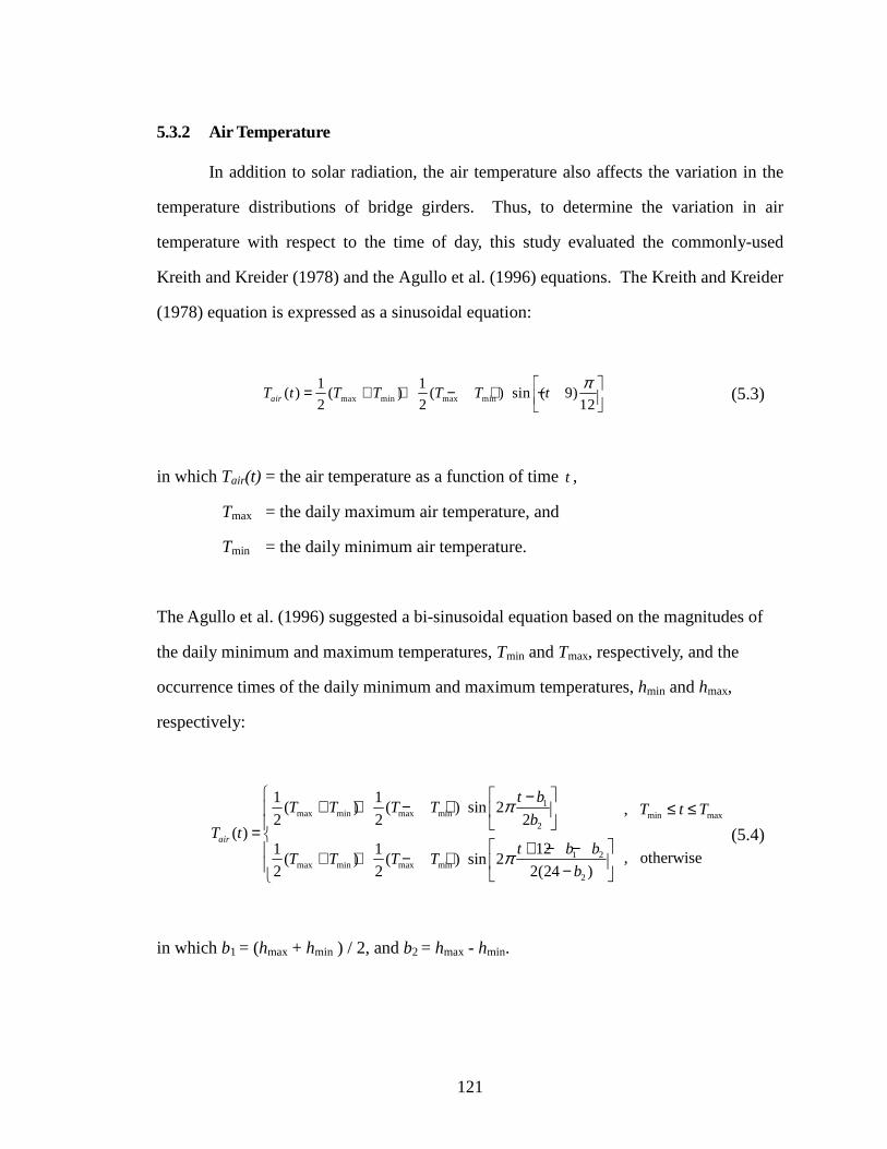
121

5.3.2 Air Temperature

In addition to solar radiation, the air temperature also affects the variation in the

temperature distributions of bridge girders. Thus, to determine the variation in air

temperature with respect to the time of day, this study evaluated the commonly-used

Kreith and Kreider (1978) and the Agullo et al. (1996) equations. The Kreith and Kreider

(1978) equation is expressed as a sinusoidal equation:

max min max min

1 1( ) ( ) ( ) sin ( 9)

2 2 12airT t T T T T tπ = + + − ⋅ −

(5.3)

in which Tair(t) = the air temperature as a function of time t ,

Tmax = the daily maximum air temperature, and

Tmin = the daily minimum air temperature.

The Agullo et al. (1996) suggested a bi-sinusoidal equation based on the magnitudes of

the daily minimum and maximum temperatures, Tmin and Tmax, respectively, and the

occurrence times of the daily minimum and maximum temperatures, hmin and hmax,

respectively:

1max min max min

2

1 2max min max min

2

1 1( ) ( ) sin 2

2 2 2( )

121 1( ) ( ) sin 2

2 2 2(24 )

air

t bT T T T

bT t

t b bT T T T

b

π

π

−+ + − ⋅ =

+ − − + + − ⋅ −

min max,

, otherwise

T t T≤ ≤ (5.4)

in which b1 = (hmax + hmin ) / 2, and b2 = hmax - hmin.

122

Variations in air temperature predicted by the two equations were compared with

those measured on June 1, October 1, and November 15, 2005. On June 1 and November

15, the largest vertical and transverse temperature differentials were measured. For the

evaluation of these equations in the spring and fall conditions, this study also included

October 1, when seasonally large vertical and transverse temperature differentials were

observed. Figure 5.5 shows the variations in air temperature predicted hourly from the

Kreith and Kreider (1978) and the Agullo et al. (1996) equations and the measured data

for the three days. The daily maximum and minimum temperatures and the occurrence

times of those temperatures employed in the models to predict variations in air

temperature were taken from the measurements.

According to Figure 5.5, the Kreith & Kreider (1978) equation provides

somewhat better correlations with the measurements on June 1 and October 1 while the

Agullo et al. (1996) equation provides better agreement with the measurements on

November 15. This difference might be attributed to the variability in air temperature

such as the magnitude of daily temperature variance, the occurrence times of daily

maximum and minimum temperatures, and instant changes in the weather condition. In

this study, the Kreith & Kreider (1978) equation was selected for the variations in air

temperature with respect to the time of day because the temperature variations predicted

from the Kreith & Kreider (1978) equation showed higher temperatures during the

morning. In addition, the Kreith & Kreider (1978) equation can predict temperature

variations simply from daily maximum and minimum air temperatures while the Agullo

et al. (1996) equation requires both the magnitudes and the times of daily minimum and

maximum temperatures.

123


Figure 5.5: Comparison of the air temperature measured every five minutes and the predicted hourly air temperature for June 1,


0 2 4 6 8 10 12 14 16 18 20 22 24

10

20

30

40

Time (hr)

Tem

pera

atur

e (o C

)

Kreith & Kreder (1978) Model

Agullo et al. (1996) Model

Measurement

50

68

86

104

0 2 4 6 8 10 12 14 16 18 20 22 24

10

20

30

40

Time (hr)



Measurement

50

68

86

104

0 2 4 6 8 10 12 14 16 18 20 22 24

10

20

30

40

Time (hr)



Measurement

50

68

86

104

Tem

pera

atur

e (o F

)

124

5.4 Extreme Seasonal Girder Temperature Variations

With the determined extremes in seasonal environmental conditions in Atlanta,

Georgia, this section investigated seasonal extremes in vertical and transverse

temperature distributions and differentials in AASHTO-PCI standard girder sections

using the 2D heat transfer analysis presented in Chapter 3. Four AASHTO-PCI sections

were selected to evaluate the variations in temperature on the AASHTO-PCI sections.

5.4.1 Finite Element Transient Heat Transfer Analysis

The AASHTO-PCI standard girder sections are composed of six I-beams and

three bulb-tees. According to the relative lengths of the top and bottom flanges, the six I-

beams are also divided into four I-beams having smaller top flanges and two I-beams

having wider top flanges. The length of the top flange of the three bulb-tees is longer

than that of the bottom flange. Based on the shapes and sizes of the AASHTO-PCI

sections, this study selected the smallest and largest sections, Type-I and Type-IV

sections, respectively, among the four I-beams with smaller top flanges. For the sections

with wider top flanges, the BT-63 section, which is the median of the depths of the three

bulb-tee sections, and the Type-V section, which is the same depth of 63 inches, were

selected. The thickness of the Type-V section is thicker than that of the BT-63 section.

Figure 5.6 shows the cross-sections of the four selected AASHTO-PCI standard girder

sections.

The finite element meshes of these four sections for heat transfer analyses are

illustrated in Figure 5.7. The size of the element was determined to be approximately one

inch long according to a temperature conversion test. Thus, Type-I section was modeled

with 342 elements and 266 nodes, Type-IV section with 696 elements and 780 nodes,

Type-V section with 880 elements and 990 nodes, and BT-63 section with 584 elements

and 699 nodes. All the models used the four-node DC2D heat transfer element in

125

ABAQUS. The orientation of the bridge sections was assumed to be the east-west

direction, in which maximum transverse temperature differentials would occur.

The thermal material properties of concrete used in these heat transfer analyses

were taken as the same values used in Chapter 3. That is, the thermal conductivity of

concrete is 1.5 W/m·K, and the specific heat of concrete is 1,000 J/kg·K. The values of

the solar absorptivity and the surface emissivity of concrete are 0.50 and 0.85,

respectively. The heat transfer boundary conditions involved in this study, such as heat

irradiation from the sun and heat radiation from the concrete surface, were described in

detail in Chapter 3. The heat transfer analyses started at 12 a.m. with a constant

temperature distribution over the cross-section. The constant initial temperature was

taken as the air temperature at 12 a.m. calculated from daily maximum and minimum

temperatures using Equation (5.3). Then, this study evaluated seasonal variations in

vertical and transverse temperature distributions in the four AASHTO-PCI sections. As

shown in Figure 5.7, the vertical temperature distributions were defined at selected nodes

along the A-A line and transverse temperature distributions along B-B, C-C, and D-D

lines for the top flange, the web, and the bottom flange, respectively.

126

(a) Type-I section (b) Type-IV section

(c) Type-V section (d) BT-63 section

Figure 5.6: The cross-sections of the AASHTO-PCI standard girder sections.

63" 63" 33" 45"

42" 42"

28" 26"

8" 6"

5" 3.5"

54"

28"

16" 26"

12"

20"

23"

11"

4"

8"

8"

5"

127

(a) Type-I section (b) Type-IV section

(c) Type-V section (d) BT-63 section Figure 5.7: The finite element meshes for the heat transfer analyses and the selected

nodes for the vertical and transverse temperature distributions.

B

C

D

B

D

C C

D D

C

B B

A

A A

A

B

C

D

B

D

A

A

C

B

C

B

C

D D

A

A

128

5.4.2 Time Interval and Period of the Heat Transfer Analysis

To determine a proper time interval in the heat transfer analysis, this study

investigated temperature variations in a BT-63 section for 5-, 15-, 30-, and 60-minute

intervals. Environmental conditions involved in this study are extreme summer

conditions in Atlanta, Georgia. Daily solar radiation is 29.4 MJ/m2, and daily maximum

and minimum temperatures defined as record daily maximum and average daily

minimum temperatures from the NCDC are 38.3°C (100.9°F) and 19.0°C (66.2°F). The

2D heat transfer analyses were performed for a consecutive three-day period, and the

influence of time intervals and time periods on temperature variations in the prestressed

concrete girder was evaluated.

Figures 5.8 to 5.10 show the temperature variations obtained from the heat

transfer analyses of the 5- and 60-minute intervals on the top surface of the top flange, in

the middle of the web, and on the bottom surface of the bottom flange, respectively.

These figures indicate that heat transfer analysis at the 60-minute interval accurately

represents the temperature variations of the prestressed concrete girder. In addition, since

concrete with a low value of thermal conductivity responds late to changes in

environmental conditions, the study analyzes the time period of heat transfer. Figure 5.11

presents the highest girder temperatures on the top surface, in the web, and on the bottom

surface of the BT-63 girder at each analysis period from the heat transfer analysis of the

5-minute interval. All the temperatures exhibit slightly low values on the first day but

show approximately the same temperatures on the second and third days. Thus, the 2D

heat transfer analysis will be performed hourly for consecutive two days, and the girder

temperatures will be determined from the second day result.

129

Figure 5.8: Temperature variations on the top surface of the BT-63 girder obtained from

the heat transfer analysis using 5- and 60-minute intervals.

Figure 5.9: Temperature variations in the middle of the BT-63 girder web obtained from

the heat transfer analysis using 5- and 60-minute intervals.

1st day 12:00 2nd day 12:00 3rd day 12:00 24:00

30

40

50

60T

empe

ratu

re (

o C)

Time (hr)

60-minute interval

5-minute interval

86

104

122

140

Tem

pera

ture

(o F

)


30

40

50

60

Time (hr)

Tem

pera

ture

(o C

)

60-minute interval

5-minute interval

86

104

122

140

Tem

pera

ture

(o F

)

130

Figure 5.10: Temperature variations on the bottom surface of the BT-63 girder obtained

from the heat transfer analysis using 5- and 60-minute intervals.

Figure 5.11: The highest temperatures on the top surface, in the middle of the web, and

on the bottom surface of the BT-63 girder at each analysis period from the

heat transfer analysis using the 60-minute interval.


30

40

50

60

Time (hr)

Tem

pera

ture

(o C

)

60-minute interval

5-minute interval

86

104

122

140

Tem

pera

ture

(o F

)

On the Top surface In the Web On the Bottom Surface20

30

40

50

60

Tem

pera

ture

(o C)

1st day

2nd day3rd day

68

86

104

122

140

Tem

pera

ture

(o F)

131

5.4.3 Seasonal Temperature Differentials

With seasonal changes in environmental conditions, the cross-sections of the

prestressed concrete girders experience variations in vertical and transverse temperature

differentials. Thus, this study examined the seasonal vertical and transverse temperature

changes from the difference between the highest and lowest temperatures in the four

selected AASHTO-PCI sections; Type-I, Type-IV, Type-V, and BT-63 sections. Vertical

temperatures were studied along the depth of the section (A-A line), and transverse

temperatures were studied across the top flange (B-B line), the web (C-C line), and the

bottom flange (D-D line).

The highest temperature along the depth of the section, A-A line, was recorded on

the top surface of the top flange, and the lowest temperature was recorded in the middle

of the bottom flange. For the transverse temperature differentials along the B-B, C-C,

and D-D lines, the highest temperatures were recorded on the south end surfaces, and the

lowest temperatures were recorded in the middle or northern side of the top flange, the

web, and the bottom flange. Tables 5.3 and 5.4 summarize the seasonal largest vertical

and transverse temperature differentials in the four sections in Atlanta, Georgia,

respectively.

According to Table 5.3, the maximum vertical temperature differentials were

21.8°C (39.3°F) to 26.7°C (48.0°F) in the summer, and the minimum vertical temperature

differentials were 11.6°C (20.9°F) to 14.4°C (26.0°F) in the winter. The fall and spring

were in the range of 17.8°C (32.1°F) to 21.6°C (38.9°F). Among the four AASHTO-PCI

sections in the summer, Type-V section showed the maximum differential of 26.7°C

(48.0°F), Type-IV and BT-63 sections 24.6°C (44.3°F) and 24.5°C (44.1°F), respectively,

and Type-I section the minimum differential of 21.8°C (39.3°F). Thus, the deeper Type-

IV, Type-V and BT-63 sections exhibited larger vertical temperature differentials.

Table 5.4 shows the largest transverse temperature differentials in the top flange,

the web, and the bottom flange of the four AASHTO-PCI sections for four seasons. The

132

transverse temperature differentials were the maximum in the winter and the minimum in

the summer. The maximum transverse temperature differentials of the four sections,

which occurred in the winter, were 16.6°C (29.9°F) to 20.1°C (36.1°F) in the top flange,

13.3°C (23.9°F) to 16.4°C (29.4°F) in the web, and 21.5°C (38.7°F) to 25.6°C (46.1°F) in

the bottom flange. The spring and the fall showed transitions in the transverse

temperature differentials from the maximum in the winter to the minimum in the summer.

The influence of the shadow on the transverse temperature differentials in the web was

also shown in the fall and the spring. While the transverse differentials of Type-I and

Type-IV sections in the web were 10.4°C (18.7°F) to 12.6°C (22.7°F), those of Type-V

and BT-63 sections were 3.7°C (6.6°F) and 5.7°C (10.3°F) because of the shadow on the

web from the long top flange. As a result, the transverse temperature differentials were

larger in the wider Type-IV, Type-V, and BT-63 sections.

In addition, Figure 5.12 shows hourly temperature variations in the Type-V

section, which showed the maximum vertical temperature differentials among the four

AASHTO-PCI sections in Atlanta, Georgia. As mentioned earlier, the highest and lowest

temperatures along the depth of the section were recorded on the top surface, denoted as

“A” Figure 5.12, and in the bottom flange, denoted as “B” in Figure 5.12, respectively.

The seasonal largest vertical temperature differentials of 26.7°C (48.0°F) in the summer,

21.6°C (38.9°F) in the spring, 20.6°C (37.1°F) in the fall, and 14.3°C (25.8°F) in the

winter occurred at 2:00 p.m.

Since the maximum transverse temperature differentials were found in the BT-63

section, the hourly variations in transverse temperatures in the top flange, the web, and

the bottom flange of the BT-63 section are presented in Figures 5.13 and 5.15,

respectively. The “A” and “B”, denoted in Figures 5.13 and 5.15, represent the locations

of the highest and lowest temperatures in each transverse temperature variation,

respectively. That is, the highest temperatures were observed on the south vertical

surfaces of the top flange, the web, and the bottom flange, and the lowest temperatures

133

were observed in the middle of the top flange and inside the northern side of the web and

the bottom flange. The transverse temperature differentials were the maximum in the

winter and the minimum in the summer. Because of the shadow of the top flange on the

web in the fall and the spring, Figure 5.14(a) and (c) show very small transverse

temperature differentials in the web. The occurrence times of the seasonal largest

transverse temperature differentials were 1:00 p.m. in the top flange and the web and 2:00

p.m. in the bottom flange.

134

Table 5.3: Seasonal largest vertical temperature differentials along the depth (A-A) of the

four AASHTO-PCI standard girder sections.

AASHTO-PCI Standard Sections

Vertical Temperature Differentials, °C (°F)

Spring Summer Fall Winter

Type-I 18.6 (33.6) 21.8 (39.3) 17.8 (32.1) 12.2 (22.0)

Type-IV 21.4 (38.5) 24.6 (44.3) 20.3 (36.6) 14.4 (26.0)

Type-V 21.6 (38.9) 26.7 (48.0) 20.6 (37.1) 14.3 (25.8)

BT-63 19.2 (34.6) 24.5 (44.1) 18.9 (34.1) 11.6 (20.9)

Table 5.4: Seasonal largest transverse temperature differentials in the top flange (B-B), in

the web (C-C), and the bottom flange (D-D) of the four AASHTO-PCI

standard girder sections.


Transverse Temperature Differentials, °C (°F)


Type-I

B-B 14.0 (25.2) 8.6 (15.5) 13.2 (23.8) 16.6 (29.9)

C-C 10.6 (19.0) 3.8 ( 6.8) 10.4 (18.7) 13.3 (23.9)

D-D 18.9 (34.0) 12.5 (22.5) 18.2 (32.8) 21.5 (38.7)

Type-IV

B-B 14.4 (25.9) 7.3 (13.2) 13.8 (24.8) 18.9 (34.1)

C-C 12.6 (22.7) 4.7 ( 8.5) 12.3 (22.2) 15.8 (28.4)

D-D 21.3 (38.4) 13.8 (24.8) 20.3 (36.5) 24.6 (44.4)

Type-V

B-B 15.9 (28.6) 8.8 (15.8) 14.7 (26.4) 20.1 (36.1)

C-C 5.7 (10.3) 5.0 ( 9.0) 5.2 ( 9.3) 16.4 (29.4)

D-D 21.2 (38.2) 12.0 (21.6) 20.2 (36.4) 24.6 (44.2)

BT-63

B-B 16.0 (28.8) 9.0 (16.3) 14.7 (26.5) 19.6 (35.3)

C-C 4.0 ( 7.2) 3.8 ( 6.9) 3.7 ( 6.6) 13.3 (23.9)

D-D 23.7 (42.7) 12.0 (21.7) 22.7 (40.9) 25.6 (46.1)

135

Figure 5.12: Vertical temperature variations along the depth of Type-V section for four seasons in Atlanta, Georgia.

2 4 6 8 10 12 14 16 18 20 22Time (hr)

A

B

32

50

68

86

104

122

140

Tem

pera

ture

(o F)

32

50

68

86

104

122

140

Tem

pera

ture

(o F)

2 4 6 8 10 12 14 16 18 20 22Time (hr)

A

B

2 4 6 8 10 12 14 16 18 20 220

10

20

30

40

50

60

Time (hr)

Tem

pera

ture

(o C)

A

B

2 4 6 8 10 12 14 16 18 20 220

10

20

30

40

50

60

Time (hr)

Tem

pera

ture

(o C)

A

B

North South

A

B

(a) Spring (b) Summer

(c) Fall (d) Winter

21.6°C (38.9°F)

20.6°C (37.1°F)

26.7°C (48.0°F)

14.3°C (25.8°F)

136

Figure 5.13: Transverse temperature variations in the top flange of BT-63 section for four seasons in Atlanta, Georgia.

2 4 6 8 10 12 14 16 18 20 220

10

20

30

40

50

60

Time (hr)

Tem

pera

ture

(o C)

A

B

2 4 6 8 10 12 14 16 18 20 220

10

20

30

40

50

60

Time (hr)

Tem

pera

ture

(o C)

A

B

2 4 6 8 10 12 14 16 18 20 22Time (hr)

A

B

32

50

68

86

104

122

140

Tem

pera

ture

(o F)

2 4 6 8 10 12 14 16 18 20 22Time (hr)

A

B

32

50

68

86

104

122

140

Tem

pera

ture

(o F)

(a) Spring

(c) Fall

16.0°C (28.8°F)

14.7°C (26.5°F)

(b) Summer

(d) Winter

9.0°C (16.3°F)

19.6°C (35.3°F)

North South

A B

137

Figure 5.14: Transverse temperature variations in the web of BT-63 section for four seasons in Atlanta, Georgia.

2 4 6 8 10 12 14 16 18 20 220

10

20

30

40

50

60

Time (hr)

Tem

pera

ture

(o C)

A

B

2 4 6 8 10 12 14 16 18 20 220

10

20

30

40

50

60

Time (hr)

Tem

pera

ture

(o C)

A

B

2 4 6 8 10 12 14 16 18 20 22Time (hr)

A

B

32

50

68

86

104

122

140

Tem

pera

ture

(o F)

2 4 6 8 10 12 14 16 18 20 22Time (hr)

A

B

32

50

68

86

104

122

140

Tem

pera

ture

(o F)

(a) Spring

(c) Fall

4.0°C (7.2°F)

3.7°C (6.6°F)

(b) Summer

(d) Winter

3.8°C (6.9°F)

13.3°C (23.9°F)

North South

A B

138

Figure 5.15: Transverse temperature variations in the bottom flange of BT-63 section for four seasons in Atlanta, Georgia.

2 4 6 8 10 12 14 16 18 20 220

10

20

30

40

50

60

Time (hr)

Tem

pera

ture

(o C)

A

B

2 4 6 8 10 12 14 16 18 20 220

10

20

30

40

50

60

Time (hr)

Tem

pera

ture

(o C)

A

B

2 4 6 8 10 12 14 16 18 20 22Time (hr)

A

B

32

50

68

86

104

122

140

Tem

pera

ture

(o F)

2 4 6 8 10 12 14 16 18 20 22Time (hr)

A

B

32

50

68

86

104

122

140

Tem

pera

ture

(o F)

(a) Spring

(c) Fall

23.7°C (42.7°F)

22.7°C (40.9°F)

(b) Summer

(d) Winter

12.0°C (21.7°F)

25.6°C (46.1°F)

North South

A B

139

5.4.4 Seasonal Vertical Temperature Distributions

Based on seasonal largest vertical temperature differentials in Atlanta, Georgia,

this study evaluated seasonal maximum vertical temperature distributions along the A-A

line for Type-I, Type-IV, Type-V, and BT-63 sections. Figures 5.16 to 5.19 show the

seasonal vertical temperature distributions of the four AASHTO-PCI sections. As

expected, the magnitudes of the temperatures were the highest in the summer and

decreased with decreases in solar radiation and air temperature from the summer to the

winter. In the fall, spring, and winter, the vertical temperature distributions showed

relatively higher increases in the web due to high solar radiation on the vertical surface.

However, for the Type-V and BT-63 sections having wider top flanges, Figures 5.18 and

5.19 exhibit no temperature increases in the top of the web in the fall and the spring

because of the shadow on the web from the top flange. The shapes of the seasonal

vertical temperature distributions were similar with no specific differences between the

four AASHTO-PCI sections.

Figures 5.20 and 5.21 show the seasonal maximum vertical temperature gradients

obtained by subtracting the lowest temperature from the maximum vertical temperature

distributions for the Type-I and BT-63 sections, respectively. The Type-I section, the

smallest section in the AASHTO-PCI sections, showed the minimum vertical temperature

differential, and the BT-63 section showed the maximum vertical temperature differential.

The vertical temperature gradients obtained from the current study were compared with

those given in the AASHTO specifications (AASHTO, 1989 & 2007), which were

obtained from solar heating only on the top surface of the bridge deck based on average

daily solar radiation for the months of June and July. Therefore, the shapes of the vertical

temperature gradients in the summer were similar to those of the AASHTO

specifications. The vertical temperature differentials in the summer also agreed well with

those of the AASHTO specifications for the small Type-I section. However, for the

140

deeper BT-63 section, the vertical temperature differentials given in the AASHTO

specifications were somewhat smaller. For the other seasons, the vertical temperature

gradients of the Type-I and BT-63 sections were different from those of the AASHTO

specifications. In the winter, because of the lowest altitude of the sun, or the highest

intensity of solar radiation on the vertical surface, largest vertical temperature gradients in

the web were found. The fall and the spring with the same solar altitude show very

similar vertical temperature gradients, which represent a transition from the summer to

the winter or from the winter to the summer. In addition, the influence of the shadow on

the vertical temperature gradient in the web was observed in the BT-63 section as shown

in Figure 5.21(b).

141

Figure 5.16: The seasonal maximum vertical temperature distributions of Type-I section.

Figure 5.17: The seasonal maximum vertical temperature distributions of Type-IV section.

10 20 30 40 50 60

0

6.25

22.2

28

Temperature (oC)

Dep

th o

f the

Typ

e-I s

ectio

n (in

)

SpringSummerFallWinter

50 68 86 104 122 140

Temperature (oF)

10 20 30 40 50 60

0

9.92

44.2

54

Temperature (oC)

Dep

th o

f the

Typ

e-IV

sec

tion

(in)


50 68 86 104 122 140

Temperature (oF)

North South

North South

142

Figure 5.18: The seasonal maximum vertical temperature distributions of Type-V section.

Figure 5.19: The seasonal maximum vertical temperature distributions of BT-63 section.

10 20 30 40 50 60

0

9.82

55

63

Temperature (oC)

Dep

th o

f the

Typ

e-V

sec

tion

(in)

Spring

SummerFall

Winter

50 68 86 104 122 140

Temperature (oF)

10 20 30 40 50 60

0

8.75

57.5

63

Temperature (oC)

Dep

th o

f the

BT

-63

sect

ion

(in)


50 68 86 104 122 140Temperature (oF)

North South

North South

143

(a) Summer and winter

(b) Fall and spring

Figure 5.20: The seasonal maximum vertical temperature gradients of Type-I section.

0 5 10 15 20 25

0

6.25

22.2

28

Temperature (oC)

Dep

th o

f the

Typ

e-I s

ectio

n (in

)

0 9 18 27 36 45

Temperature (oF)

AASHTO (1989)AASHTO (2007)Current Study: SummerCurrent Study: Winter

0 5 10 15 20 25

0

6.25

22.2

28

Temperature (oC)

Dep

th o

f the

Typ

e-I s

ectio

n (in

)

0 9 18 27 36 45

Temperature (oF)

AASHTO (1989)AASHTO (2007)Current Study: FallCurrent Study: Spring

North South

North South

144

(a) Summer and winter

(b) Fall and spring

Figure 5.21: The seasonal maximum vertical temperature gradients of BT-63 section.

0 5 10 15 20 25

0

10.5

57.5

63

Temperature (oC)

Dep

th o

f th

e B

T-6

3 se

ctio

n (in

)

0 9 18 27 36 45

Temperature (oF)

AASHTO (1989)

AASHTO (2007)

Current Study: Summer

Current Study: Winter

0 5 10 15 20 25

0

10.5

57.5

63

Temperature (oC)

Dep

th o

f th

e B

T-6

3 se

ctio

n (in

)

0 9 18 27 36 45

Temperature (oF)

AASHTO (1989)

AASHTO (2007)Current Study: Spring

Current Study: Fall North South

North South

145

5.4.5 Seasonal Transverse Temperature Distributions

This study also investigated seasonal maximum transverse temperature

distributions and gradients across the top flange, the web, and the bottom flange of the

BT-63 girder, in which the maximum transverse temperature differentials were observed.

Figure 5.22 shows the seasonal maximum transverse temperature distributions in the top

flange. The highest temperature was found on the south end surface, and the lowest

temperature was found in the middle of the top flange. The magnitudes of the

temperatures were the highest in the summer, the second highest in the fall, and the

smallest in the winter. However, the transverse temperature gradient of the top flange as

shown in Figure 5.23 is the largest in the winter, the second largest in the fall and the

spring, and the smallest in the summer. The seasonal largest transverse temperature

differentials in the top flange obtained from seasonal extreme environmental conditions

in Atlanta, Georgia are 19.6°C (35.3°F) in the winter, 16.0°C (28.8°F) and 14.7°C

(26.5°F) in the spring and the fall, respectively, and 9.0°C (16.2°F) in the summer.

Figure 5.24 shows the seasonal maximum transverse temperature distributions in

the web of the BT-63 section. As expected, the high magnitudes of the temperatures were

observed in the summer and the fall. The transverse temperature gradients as shown in

Figure 5.25 are the maximum in the winter due to high solar radiation on the vertical

surface. In the fall and the spring, unlike the large transverse temperature gradients in the

top and bottom flanges, the web exhibited no increases in the transverse gradients due to

the shadow on the web. The seasonal largest transverse temperature differentials of the

web in Atlanta, Georgia is 13.3°C (23.9°F) in the winter and about 4°C (7°F) in the other

seasons.

For the bottom flange, the seasonal maximum transverse temperature distributions

and gradients are shown in Figures 5.26 and 5.27, respectively. As mentioned earlier, the

magnitudes of the temperatures increased from the winter to the summer. However, in

the summer, the temperature magnitudes in the south part of the bottom flange were small

146

because the shadow of the top flange extended to the bottom flange. Thus, the transverse

temperature gradients were the minimum in the summer as shown in Figure 5.27. The

seasonal largest transverse temperature differentials of the bottom flange in Atlanta,

Georgia are 25.6°C (46.1°F) in the winter, 23.7°C (42.7°F) and 22.7°C (40.9°F) in the

fall and spring, respectively, and 12.0°C (21.7°F) in the winter.

147

Figure 5.22: Seasonal maximum transverse temperature distributions in the top flange of

BT-63 section.

Figure 5.23: Seasonal maximum transverse temperature gradients in the top flange of

BT-63 section.

0 21 42

10

20

30

40

50

60

Tem

pera

ture

(o C)

Width of Top Flange (in)

Spring

SummerFall

Winter

32

50

68

86

104

122

Tem

pera

ture

(o F)

0 21 42

0

5

10

15

20

25

Tem

pera

ture

(o C)


Spring

Summer

Fall

Winter

0

9

18

27

36

45T

empe

ratu

re (o F

)

North South

North South

148

Figure 5.24: Seasonal maximum transverse temperature distributions in the web of BT-

63 section.

Figure 5.25: Seasonal maximum transverse temperature gradients in the web of BT-63

section.

0 3 6

20

25

30

35

40T

empe

ratu

re (o C

)

Width of the BT-63 Section (in)

Spring

SummerFall

Winter

68

77

86

95

104

Tem

pera

ture

(o F)

0 3 6

0

5

10

15

20

Tem

pera

ture

(o C)

Width of Web (in)

Spring

SummerFall

Winter

0

9

18

27

36T

empe

ratu

re (o F

)

South North

North South

149

Figure 5.26: Seasonal maximum transverse temperature distributions in the bottom

flange of BT-63 section.

Figure 5.27: Seasonal maximum transverse temperature gradients in the bottom flange of

BT-63 section.

0 13 26

10

20

30

40

50

60

Tem

pera

ture

(o C)

Width of Bottom Flange (in)

Spring

SummerFall

Winter

50

68

86

104

122

140

Tem

pera

ture

(o F)

0 13 26

0

5

10

15

20

25

30

Tem

pera

ture

(o C)


Spring

SummerFall

Winter

0

9

18

27

36

45

54T

empe

ratu

re (o F

)

North South

North South

150

5.5 Influences of Bridge Axes on the Temperature Distributions

This study investigated seasonal variations in the vertical and transverse

temperature distributions of prestressed concrete bridge girders in an east-west

orientation. This orientation was assumed to provide maximum transverse temperature

distributions in the bridge girders since only one side of the girders directly receive solar

radiation from the sun. Thus, this section evaluated variations in the temperature

distributions with changes in bridge orientations using 2D heat transfer analysis. Since

the largest vertical and transverse temperature distributions were found in Type-V and

BT-63 sections, this analytical study was carried out on these two sections under seasonal

extremes in environmental conditions in Atlanta, Georgia. The bridge orientations

involved in this study are east-west (E-W), southwest-northeast (SW-NE), south-north (S-

N), and southeast-northwest (SE-NW) orientations shown in Figure 5.28.

Figure 5.28: Bridge orientations involved in this study.

Southwest-Northeast Orientation Southeast-Northwest

Orientation

East-West Orientation

South-North Orientation

151

5.5.1 Vertical Temperature Differentials and Gradients

Tables 5.5 and 5.6 summarize the seasonal largest vertical temperature

differentials obtained from the heat transfer analysis in the Type-V and BT-63 sections,

respectively, for four bridge orientations. Since vertical temperature variations in the

bridge girder mainly depend on the intensity of solar radiation on the top surface of the

girder, the vertical temperature differentials were the largest in the summer, the second

largest in the fall and spring, and the smallest in the winter. For the same reason, the

changes in bridge orientations only slightly affected the vertical temperature differentials.

As shown in Tables 5.5 and 5.6, the maximum vertical temperature differentials, 26.7°C

(48.0°F) in Type-V section and 24.5°C (44.1°F) in BT-63 section, occurred in the summer

and in the E-W orientation. With changes in bridge orientations from the E-W to the SE-

NW, variances in the vertical temperature differentials were less than 3.7°C (6.7°F). The

occurrence times of the vertical temperature differentials were 2:00 p.m. in all the seasons

and orientations.

Based on the maximum vertical temperature differentials which occurred in the

summer, Figure 5.29 shows the maximum vertical temperature gradients obtained by

subtracting a lowest temperature from the girder temperatures for four bridge

orientations. The vertical temperature gradients as shown in Figure 5.29 decreased from

the top surface of the top flange to the bottom flange. In particular, the top flange showed

a rapid decrease in the vertical temperature gradient. The largest differentials of the

vertical gradient were observed in the E-W orientation. With changes in bridge

orientations, the values of the vertical differentials slightly changed, and the shapes of the

vertical gradients were almost the same.

Figure 5.29 also compared the vertical temperature gradients obtained from the

current study and those recommended in the AASHTO specifications (1989, 2007). As

discussed in Section 5.4.4, the AASHTO specifications exhibit smaller vertical

temperature differentials for the deeper AASHTO-PCI sections, Type-V and BT-63

152

sections. In addition, while the AASHTO specifications define a minimum temperature,

or a zero point of the vertical gradient, in the web or in the bottom of the top flange, this

study shows the zero point in the middle of the bottom flange. Thus, for the design of

prestressed concrete bridge girders, a simplified vertical temperature gradient was

proposed in terms of the locations of the top flange, the web, and the bottom flange of

prestressed concrete girders as shown in Figure 5.30. The proposed vertical gradient

decreases from the highest temperature on the top surface to the zero temperature in the

middle of the bottom flange. The vertical temperature differentials, denoted T1 and T2 in

Figure 5.30, were determined to be 27°C (49°F) and 5°C (9°F), respectively, based on

extreme summer environmental conditions in Atlanta, Georgia.

Table 5.5: Seasonal largest vertical temperature differentials in Type-V section

with respect to four bridge orientations.

Bridge Orientations Vertical Temperature Differentials, °C (°F)

Spring Summer Fall Winter East-West

(E-W) 21.6 (38.9) at 2 p.m.

26.7 (48.0) at 2 p.m.

20.6 (37.1) at 2 p.m.

14.3 (25.8) at 2 p.m.

Southwest-Northeast (SW-NE)

21.4 (38.5) at 2 p.m.

24.1 (43.3) at 2 p.m.

20.4 (36.7) at 2 p.m.

14.9 (26.8) at 2 p.m.

South-North (S-N)

22.1 (36.7) at 2 p.m.

23.8 (42.9) at 2 p.m.

23.3 (41.9) at 2 p.m.

17.4 (31.4) at 2 p.m.

Southeast-Northwest (SE-NW)

23.5 (42.4) at 2 p.m.

24.6 (44.3) at 2 p.m.

22.6 (40.6) at 2 p.m.

17.5 (31.6) at 2 p.m.

Table 5.6: Seasonal largest vertical temperature differentials in BT-63 section

with respect to four bridge orientations.

Bridge Orientations Vertical Temperature Differentials, °C (°F)


East-West (E-W)

19.2 (34.6) at 2 p.m.

24.5 (44.1) at 2 p.m.

18.9 (34.1) at 2 p.m.

11.6 (20.9) at 1 p.m.

Southwest-Northeast (SW-NE)

17.8 (32.0) at 2 p.m.

20.8 (37.4) at 2 p.m.

17.3 (31.1) at 2 p.m.

11.0 (19.7) at 2 p.m.

South-North (S-N)

18.9 (34.0) at 2 p.m.

21.0 (37.8) at 2 p.m.

20.4 (36.8) at 2 p.m.

14.8 (26.6) at 2 p.m.

Southeast-Northwest (SE-NW)

21.2 (38.2) at 2 p.m.

22.3 (40.1) at 2 p.m.

20.5 (36.9) at 2 p.m.

15.6 (28.0) at 2 p.m.

153

(a) Type-V section

(b) BT-63 section

Figure 5.29: Maximum vertical temperature gradients with respect to four bridge

orientations in the summer.

0 5 10 15 20 25

0

9.82

55

63

Temperature (oC)

Dep

th o

f th

e T

ype-

V s

ectio

n (in

)

AASHTO (1989)

AASHTO (2007)

East-WestSouthwest-Northeast

South-North

Southeast-Northwest

0 9 18 27 36 45

Temperature (oF)

0 5 10 15 20 25

0

8.75

57.5

63

Temperature (oC)

Dep

th o

f th

e B

T-6

3 se

ctio

n (in

)

AASHTO (1989)AASHTO (2007)

East-West

Southwest-Northeast

South-NorthSoutheast-Northwest

0 9 18 27 36 45

Temperature (oF)

154

Figure 5.30: A proposed vertical temperature gradient along the depth of prestressed

concrete bridge girders.

5.5.2 Transverse Temperature Differentials and Gradients in the Top Flange

In addition, the influence of bridge orientations on transverse temperature

differentials in the top flange of prestressed concrete bridge girders was investigated.

Since larger transverse temperature differentials were found in the wider Type-V and BT-

63 sections, this study evaluated seasonal largest transverse temperature differentials in

the top flange of the Type-V and BT-63 sections for each bridge orientation. The

maximum transverse temperature differentials were found in the both E-W orientation

and the winter; 20.1°C (36.1°F) for Type-V section and 19.6°C (35.3°F) for BT-63

section. In general, large transverse temperature differentials were observed in the E-W

and SW-NE orientations, in which bridge girders are more exposed to the sun than the S-

N and the SE-NW orientations. With seasonal changes, the transverse temperature

T1 = 27°C (49°F)

T2 = 5°C (9°F)

Top flange

Bottom flange

Girder Depth

T3 ≤ 3°C (5°F)

Web

155

differentials were the largest in the winter because of high solar radiation on the vertical

surface.

For the S-N orientation, the transverse temperature differentials of the top flange,

shown in Table 5.7 for Type-V section and Table 5.8 for BT-63 section, were similar with

no specific seasonal variations. Moreover, the transverse differentials in the winter, even

though high solar intensity on the vertical surface, showed smaller values because of

smaller time exposed to the sun. The transverse temperature differentials in the SE-NW

orientation, in which bridge girders are exposed to the sun for only a couple of hours in

the morning, were negligible.

Figure 5.31 also shows the transverse temperature gradients for each orientation

in which maximum transverse gradients were observed in the E-W orientation. The

transverse gradients increased only in half of the top flange. The gradient in the other

side were nearly constant. Therefore, based on the transverse gradients and differentials

obtained from extreme winter environmental conditions in Atlanta, Georgian, in the E-W

orientation, this study proposed a transverse temperature gradient for the top flange as

shown in Figure 5.32. The transverse gradient proposed in this study increases from the

middle of the top flange to a maximum differential of 20°C (36°F) at the end of the one

side. Temperature T1 shown in Figure 5.32 was determined to be one-fourth of the

maximum temperature differential of 20°C (36°F). The one-fourth temperature, defined

as the middle temperature of the transverse gradient, agrees well with the second-order

model proposed for transverse temperature distributions in prestressed concrete bridge

girders. Between the temperature differentials of T1, 20°C (36°F), and T2, 5°C (9°F),

shown in Figure 5.32, the transverse temperature gradient was assumed to be linear.

156

Table 5.7: Seasonal largest transverse temperature differentials in the top flange of Type-

V section with respect to four bridge orientations.

Bridge Orientations Transverse Temperature Differentials: Top Flange, °C (°F)


East-West 15.9 (28.6) at 2 p.m.

8.5 (15.3) at 1 p.m.

14.7 (26.4) at 1 p.m.

20.1 (36.1) at 2 p.m.

Southwest-Northeast 15.9 (28.6) at 12 p.m.

10.5 (18.9) at 11 a.m.

15.0 (27.1) at 11 a.m.

17.6 (31.7) at 12 p.m.

South-North 13.5 (24.3) at 11 a.m.

12.0 (21.6) at 10 a.m.

12.9 (23.3) at 10 a.m.

11.0 (22.4) at 11 a.m.

Southeast-Northwest 7.1 (12.8) at 9 a.m.

9.6 (17.2) at 9 a.m.

6.8 (12.2) at 9 a.m.

2.7 (4.8) at 9 a.m.

Table 5.8: Seasonal largest transverse temperature differentials in the top flange of BT-63

section with respect to four bridge orientations.

Bridge Orientations Transverse Temperature Differentials: Top Flange, °C (°F)


East-West 16.0 (28.8) at 1 p.m.

9.0 (16.3) at 1 p.m.

14.7 (26.5) at 1 p.m.

19.6 (35.3) at 1 p.m.


11.0 (19.8) at 11 a.m.

14.7 (26.5) at 11 a.m.

16.6 (29.8) at 12 p.m.


12.2 (22.0) at 10 a.m.

13.0 (23.4) at 10 a.m.

11.4 (20.5) at 11 a.m.


9.7 (17.5) at 9 a.m.

7.1 (12.7) at 9 a.m.

3.1 (5.6) at 9 a.m.

157

(a) Type-V section

(b) BT-63 section

Figure 5.31: Maximum transverse temperature gradients in the top flange with respect to

four bridge orientations in the winter.

0 21 42

0

5

10

15

20

25

Tem

pera

ture

(o C)


East-West

Southwest-NortheastSouth-North

Southeast-Northwest

0

9

18

27

36

45

Tem

pera

ture

(o F)

0 21 42

0

5

10

15

20

25

Tem

pera

ture

(o C)


East-West


Southeast-Northwest

0

9

18

27

36

45

Tem

pera

ture

(o F)

158

Figure 5.32: A proposed transverse temperature gradient in the top flange of prestressed


5.5.3 Transverse Temperature Differentials and Gradients in the Web

The effects of changes in bridge orientations on transverse temperature

differentials in the girder web were also evaluated. Tables 5.9 and 5.10 summarize the

seasonal largest transverse temperature differentials in the web of BT-63 and Type-IV

sections, respectively, with changes in bridge orientations. Since the web of the bridge

girder is more exposed to the sun in an E-W orientation and solar radiation incident on

the vertical surface is the highest in the winter, the maximum transverse temperature

differentials of 16.4°C (29.4°C) in the Type-V section and 13.2°C (23.9°F) in the BT-63

section occurred in the E-W orientation and in the winter.

For the S-N orientation, the transverse temperature differentials were slightly

higher in the fall and the spring with higher solar radiation on the vertical surface and

slightly smaller in the winter with less amount of time exposed to the sun. However, in

general, the transverse temperature differentials in the S-N orientation were similar in all

T1

Btop = 1/4×width of top flange

Btop Btop

T2 = 1/4× T1

Wtop = width of top flange

159

the seasons. The SE-NW orientation, as mentioned earlier, represented a slight change in

transverse temperature differentials that could be neglected.

The transverse temperature gradients of the web are presented in Figure 5.33 with

respect to four bridge orientations for the winter, in which the maximum transverse

gradient was found. Similar to the transverse temperature gradient of the top flange, the

surface more exposed to the sun experienced a rapid increase in the transverse gradient.

The temperatures in the middle of the web were approximately one quarter of the largest

temperature, which also provide good agreement with the second-order model of the

transverse temperature distribution. Therefore, based on the analytical results obtained

from the both E-W orientation and extreme winter environmental conditions in Atlanta,

Georgia, this study proposed a transverse temperature gradient across the web of

prestressed concrete bridge girders as shown in Figure 5.34. The maximum surface

temperature T1 was determined to be a maximum differential of 16°C (29°F), and the

middle temperature T2 was determined to be 4°C (7°F), one-fourth of the maximum

differential. The temperatures between the temperatures T1 and T2 were assumed to be

linear.

160

Table 5.9: Seasonal largest transverse temperature differentials in the web of Type-V


Bridge Orientations Transverse Temperature Differentials: Web, °C (°F)


East-West 5.7 (10.3) at 1 p.m.

5.0 ( 9.0) at 1 p.m.

5.2 ( 9.3) at 1 p.m.

16.4 (29.4) at 1 p.m.

Southwest-Northeast 13.7 (24.7) at 11 a.m.

9.3 (16.8) at 10 a.m.

13.5 (24.2) at 11 a.m.

14.8 (26.7) at 11 a.m.


11.8 (21.3) at 9 a.m.

12.6 (22.7) at 9 a.m.

10.2 (18.3) at 10 a.m.


9.8 (17.7) at 9 a.m.

6.8 (12.2) at 8 a.m.

2.1 (3.8) at 8 a.m.

Table 5.10: Seasonal largest transverse temperature differentials in the web of BT-63


Bridge Orientations Transverse Temperature Differentials: Web, °C (°F)


East-West 4.0 ( 7.2) at 1 p.m.

3.8 ( 6.9) at 1 p.m.

3.7 ( 6.6) at 1 p.m.

13.3 (23.9) at 1 p.m.

Southwest-Northeast 11.7 (21.0) at 11 a.m.

8.1 (14.5) at 10 a.m.

11.8 (21.2) at 10 a.m.

12.7 (22.9) at 11 a.m.


10.5 (18.8) at 9 a.m.

11.3 (20.4) at 9 a.m.

8.9 (16.0) at 10 a.m.


8.6 (15.5) at 8 a.m.

6.2 (11.2) at 8 a.m.

2.1 (3.7) at 8 a.m.

161

(a) Type-V section

(b) BT-63 section

Figure 5.33: Maximum transverse temperature gradients in the web with respect to four

bridge orientations in the winter.

0 4 8

0

5

10

15

20

Tem

pera

ture

(o C)

Width of Web (in)

East-West


Southeast-Northwest

0

9

18

27

36

Tem

pera

ture

(o F)

0 3 6

0

5

10

15

20

Tem

pera

ture

(o C)

Width of Web (in)

East-West


Southeast-Northwest

0

9

18

27

36

Tem

pera

ture

(o F)

162

Figure 5.34: A transverse temperature gradient in the web of prestressed concrete bridge

girders.

5.5.4 Transverse Temperature Differentials and Gradients in the Bottom Flange

For the bottom flange, Tables 5.11 and 5.12 show the seasonal largest transverse

temperature differentials of Type-V and BT-63 sections for the four bridge orientations.

As discussed previously, the E-W and SW-NE orientations in the winter yield maximum

transverse temperature differentials of 24.6°C (44.2°F) in the Type-V section and 25.6°C

(46.1°F) in the BT-63 section. The S-N orientation presents nearly similar transverse

differentials in all the seasons except for the winter, which showed a little smaller value

due to smaller hours exposed to the sun. The SE-NW orientation, in which bridge girders

receive solar radiation directly from the sun for only a few hours, presented the smallest

transverse differentials in the bottom flange. In particular, in the winter, the bridge

girders in the SE-NW orientation are much less exposed to the sun, so the transverse

differentials shown in Tables 5.11 and 5.12 are negligible.

Figure 5.35 shows the transverse temperature gradients in the bottom flange of the

Type-V and BT-63 sections for the four bridge orientations in the winter. As mentioned

T1

Bweb = ½ × width of web

T2 = 1/4× T1

Bweb Bweb

Wweb = width of web

163

earlier, large transverse gradients occurred in the E-W and SW-NE orientations. The

minimum temperature of the transverse gradient, or a zero point of the gradient, was

observed at around one fourth of the width of the bottom flange as shown in Figure 5.35.

Based on the maximum transverse gradients obtained in the E-W orientation and in the

extreme winter environmental condition in Atlanta, Georgia, Figure 5.36 shows a

transverse temperature gradient for the bottom flange of prestressed concrete bridge

girders. The maximum differential of T1 was determined to be 26°C (47°F), and the

temperatures of T2 and T3 were determined to be 12°C (21°F) and 3°C (5F), respectively.

The transverse temperature gradient of the bottom flange proposed in this study also

matched well the second-order model of the transverse temperature distribution.

164


Type-V section with respect to four bridge orientations.

Bridge Orientations Transverse Temperature Differentials: Bottom Flange, °C (°F)


East-West 21.2 (38.2) at 2 p.m.

12.0 (21.6) at 2 p.m.

20.2 (36.4) at 2 p.m.

24.6 (44.2) at 2 p.m.


14.8 (26.6) at 12 p.m.

19.4 (34.8) at 12 p.m.

20.7 (37.3) at 1 p.m.


16.5 (29.7) at 11 a.m.

14.8 (26.6) at 10 a.m.

12.0 (21.7) at 11 a.m.


12.4 (22.4) at 9 a.m.

8.6 (15.5) at 10 a.m.

3.4 (6.2) at 10 a.m.


BT-63 section with respect to four bridge orientations.

Bridge Orientations Transverse Temperature Differentials: Bottom Flange, °C (°F)


East-West 23.7 (42.7) at 2 p.m.

12.0 (21.7) at 2 p.m.

22.7 (40.9) at 2 p.m.

25.6 (46.1) at 2 p.m.


17.7 (31.9) at 12 p.m.

21.6 (38.8) at 12 p.m.

22.1 (39.8) at 12 p.m.


18.8 (33.8) at 11 a.m.

14.4 (25.9) at 10 a.m.

12.0 (21.6) at 11 a.m.


14.1 (25.3) at 9 a.m.

10.3 (18.6) at 10 a.m.

3.9 (7.0) at 10 a.m.

165

(a) Type-V section

(b) BT-63 section

Figure 5.35: Maximum transverse temperature gradients in the bottom flange with

respect to four bridge orientations in the winter.

0 14 28

0

5

10

15

20

25

Tem

pera

ture

(o C)


East-West


Southeast-Northwest

0

9

18

27

36

45

Tem

pera

ture

(o F)

0 13 26

0

5

10

15

20

25

Tem

pera

ture

(o C)


East-West


Southeast-Northwest

0

9

18

27

36

45

Tem

pera

ture

(o F)

166

Figure 5.36: A transverse temperature gradient in the bottom flange of prestressed


5.6 Thermal Differentials at Selected Cities in the United States

The vertical and transverse temperature differentials suggested in this study were

based on extreme environmental conditions in Atlanta, Georgia. Thus, this section

further evaluates extreme summer and winter environmental conditions in the United

States. As mentioned previously, the summer and the winter are based on the months of

June and December. The extreme environmental conditions were applied to the 2D finite

element heat transfer analysis, and the vertical and transverse temperature differentials

were investigated.

5.6.1 Extreme Environmental Conditions in the United States

The experimental data taken from April 2009 to March 2010 showed that when

the large vertical and transverse temperature differentials were measured, daily solar

radiation showed a good correlation with the NSRDB 30-year (from 1961 to 1990)

T1

T2 = 4/9 × T1

Bbot = ¼ × width of bottom flange

Bbot

T3 = 1/9 × T1

Bbot Bbot

Wbot = width of bottom flange

167

monthly average daily solar radiation under clear sky conditions. Daily maximum and

minimum temperatures correlated well with the record daily maximum temperature and

the average daily minimum temperature of the NCDC climatic data, respectively.

In addition, with seasonal changes from the summer to the winter, the largest

vertical temperature differential was observed in the summer and the largest transverse

temperature differential in the winter. Thus, for the months of June and December,

representative months of the summer and the winter, this study explored the NSRDB and

NCDC data at a total of 235 cities and selected eight cities involving extreme

environmental conditions such as the highest daily solar radiation, the highest record

daily maximum temperature, and the largest daily temperature variance. Table 5.13

shows the environmental conditions extracted from the NSRDB and the NCDC for the

eight cities. For June, the highest daily solar radiation in the United States was 32.5

MJ/m2 in Alamosa, Colorado, and the highest record daily maximum temperature was

50.0°C (122°F) in Phoenix, Arizona. The largest daily temperature variance of 32.3°C

(58.3°F) was found in Medford, Oregon. In addition, Atlanta, Georgia, was included in

the current study. Similarly, in the winter, the highest daily solar radiation of 18.4 MJ/m2

was observed in Hilo, Hawaii, and the highest record daily maximum temperature of

34.4°C (94°F), was observed in Brownsville, Texas. Caribou, Maine, and Annette,

Alaska, which have extremely cold environmental conditions in the winter, were also

included. Figure 5.37 illustrates the cities involving extremes in environmental

conditions in the summer and the winter in the United States.

The determined extreme daily environmental conditions shown in Table 5.13 were

hourly distributed over the length of the days; June 21 for the summer and December 21

for the winter. The days of June 21 and December 21, representative days of the summer

and the winter, have the longest and shortest days of the year. For variations in daily

solar radiation with respect to the time of the day, the Liu and Jordan (1960) equation was

used to calculate hourly solar radiation incident on the surfaces of the girders. Variations

168

in daily air temperature were obtained from the Kreith and Kreider (1978) equation. The

effect of wind speed on the maximum temperature differentials was disregarded.

Table 5.13: Extremes in summer and winter environmental conditions for the eight cities

in the United States.

Cities Seasons b

Daily Solar

Radiation, MJ/m2

Record Daily

Maximum, °C (°F)

Average Daily Minimum,

°C (°F)

Daily Variance a,

°C (°F)

Alamosa, CO (37.45°N, 105.87°W)

Summer 32.5 33.8 ( 93) 5.0 (41.0) 28.8 (52.0)

Winter 11.2 16.1 (61) -18.1 (-0.5) 34.2 (61.5)

Phoenix, AZ (33.43°N,

1112.02°W)

Summer 31.3 50.0 (122) 22.7 (72.9) 27.3 (49.1)

Winter 12.3 31.1 (88) 5.4 (41.8) 25.7 (46.2)

Medford, OR (42.73°N, 122.87°W)

Summer 30.9 42.7 (109) 10.4 (50.7) 32.3 (58.3)

Winter 7.7 22.2 (72) - 0.4 (31.2) 22.6 (40.8)

Atlanta, GA (33.65°N, 84.43°W)

Summer 29.4 38.3 (101) 19.0 (66.2) 19.3 (34.8)

Winter 11.9 26.1 (79) 1.7 (35.0) 24.4 (44.0)

Brownsville, TX (25.90°N, 97.43°W)

Summer 28.5 38.9 (102) 23.8 (74.9) 15.1 (27.1)

Winter 15.1 34.4 (94) 11.3 (52.4) 23.1 (41.6)

Caribou, ME (46.87°N, 68.02°W)

Summer 30.5 35.6 ( 96) 9.5 (49.1) 23.8 (46.9)

Winter 6.2 14.4 (58) -14.7 ( 5.5) 29.1 (52.5)

Hilo, HI (19.72°N, 155.07°W)

Summer 29.4 32.2 ( 90) 19.8 (67.6) 12.4 (22.4)

Winter 18.4 33.9 (93) 18.2 (64.8) 15.7 (28.2)

Annette, AK (55.03°N, 131.57°W)

Summer 29.9 31.7 ( 89) 8.8 (47.8) 22.9 (41.2)

Winter 2.6 16.7 (62) - 0.3 (31.4) 17.0 (30.6)

a The daily variance was the difference between the record daily maximum temperature and the average daily minimum temperatures.

b The summer and the winter are based on the months of June and December.

169

Figure 5.37: Selected cities pertaining to extreme summer and winter environmental

conditions in the United States.

5.6.2 Vertical and Transverse Temperature Differentials

With the extreme environmental conditions, the 2D heat transfer analyses were

performed to determine maximum vertical and transverse temperature differentials for the

eight cities of the United States. With changes in bridge orientations, the E-W orientation

provided the largest vertical and transverse temperature differentials in AASHTO-PCI

standard sections. Moreover, among the AASHTO-PCI sections, Type-V and BT-63

sections showed larger vertical and transverse differentials than the other AASHTO-PCI

sections. Indeed, the Type-V section, a little thicker than the BT-63 section, exhibited

somewhat larger vertical and transverse temperature differentials. Therefore, for the

Type-V section in the E-W orientation, maximum vertical and transverse temperature

differentials were evaluated under extremes environmental conditions in the summer and

the winter, respectively, for the eight cities of the United States.

Alamosa

Phoenix

Medford

Brownsville

Atlanta

Caribou Annette

Hilo

170

Table 5.14 shows the vertical and transverse temperature differentials obtained

from the 2D heat transfer analyses. The vertical temperature differentials were a

maximum of 31.1°C (56.0°F) in Alamosa, Colorado, and a minimum of 22.6°C (40.7°F)

in Annette, Alaska. In general, the vertical temperature differentials were around 30°C

(54°F) in Medford, Oregon, Alamosa, Colorado, and Phoenix, Arizona, located in the

Western United States, and around 26°C (47°F) in Brownsville, Texas, Atlanta, Georgia,

and Caribou, Main, located in the Eastern United States. The city of Hilo, Hawaii, was

24°C (43°F), and Annette, Alaska, was 23°C (41°F).

The maximum transverse temperature differentials, 24°C (43°F) in the top flange,

19°C (34°F) in the web, and 29°C (52°F) in the bottom flange, also occurred in Alamosa,

Colorado. The remaining cities of the continental United States, Phoenix, Arizona,

Medford, Oregon, Alamosa, Colorado, Atlanta, Georgia, and Brownsville, Texas, were in

the range of 18°C (32°F) to 21°C (38°F) in the top flange, 15°C (27°F) to 17°C (31°F) in

the web, and 22°C (40°F) to 25°C (45°F) in the bottom flange. The transverse

differentials in Hilo, Hawaii, were 16°C (29°F), 15°C (27°F), and 22°C (40°F) in the top

flange, in the web, and in the bottom flange, respectively. Annette, Alaska, showed

transverse temperature differentials of 13°C (23°F) in the top flange, 11°C (20°F) in the

web, and 15°C (27°F) in the bottom flange.

In conclusion, since both maximum vertical and transverse temperature

differentials were observed in Alamosa, Colorado, the vertical thermal differential

defined in Atlanta, Georgia, increases from 27°C (49°F) to 31°C (56°F). The T2, the

temperature at the bottom of the top flange shown in Figure 5.30, is the same 5°C (9°F)

as defined in Atlanta, Georgia. The transverse temperature differentials increase to 24°C

(44°F) for the top flange, 19°C (35°F) for the web, and 29°C (53°F) for the web. Figures

5.38 and 5.39 show the vertical and transverse temperature gradients proposed in this

study for the thermal design of prestressed concrete bridge girders in the United States.

171

Table 5.14: Vertical and transverse temperature differentials for the eight cities of the

United States.

Cities Vertical

Differentials, °C (°F)

Transverse Differentials, °C (°F)


Alamosa, CO 31.1 (56.0) 24.2 (43.5) 19.2 (34.6) 29.3 (52.7)

Phoenix, AZ 29.6 (53.3) 20.5 (36.9) 16.8 (30.2) 25.3 (45.5)

Medford, OR 29.9 (53.7) 18.3 (33.0) 15.1 (27.1) 22.0 (39.6)

Atlanta, GA 26.7 (48.0) 20.1 (36.1) 16.4 (29.4) 24.6 (44.2)

Brownsville, TX 25.6 (46.0) 18.2 (32.8) 15.2 (27.4) 23.3 (41.9)

Caribou, ME 27.2 (48.9) 20.9 (37.6) 16.9 (30.5) 24.3 (43.7)

Hilo, HI 23.8 (42.9) 16.4 (29.4) 14.6 (26.2) 22.0 (39.5)

Annette, AK 22.6 (40.7) 13.0 (23.4) 10.9 (19.6) 15.0 (27.0)

Figure 5.38: The design vertical temperature gradient along the depth of prestressed

concrete bridge girders in the United States.

T1 = 31°C (56°F)

T2 = 5°C (9°F)

Top flange

Bottom flange

Girder Depth

T3 ≤ 3°C (5°F)

Web

172

(a) Top flange (b) Web (c) Bottom flange

Figure 5.39: Design transverse temperature gradients of prestressed concrete bridge girders in the United States (Not to scale).

Bbot = ¼ × width of bottom flange

T1 = 29°C (53°F)

T2= 13°C (24°F)

T3= 3°C (6°F)

T1 = 19°C (35°F)

Bweb = ½ × width of web Btop = 1/4×width of top flange

T1= 24°C (44°F)

T2 =5°C (9°F) T2= 6°C (11°F)

Btop Btop Bweb Bweb Bbot Bbot Bbot

173

CHAPTER 6

STRUCTURAL BEHAVIOR OF A PRESTRESSED CONCRETE

BRIDGE GIRDER DURING CONSTRUCTION

6.1 Introduction

The largest vertical and transverse temperature gradients were found to occur in

the deeper and wider cross-sections of the Type-V and BT-63. The BT-63 girder was then

selected for further thermal response analyses in an east-west orientation for extreme

summer and winter environmental conditions in Atlanta, Georgia. A three-dimensional

(3D) nonlinear finite element analysis was performed to evaluate the combined effects of

the thermal response, initial imperfections, and support conditions on the behavior of the

prestressed concrete girder during construction. Furthermore, a simple beam model was

developed for calculating vertical and transverse thermal movements induced by

nonlinear temperature gradients for simply supported girders.

6.2 3D Finite Element Thermal Response Analysis

The thermal response analysis is composed of a static analysis and its subsequent

thermal stress analysis. The 3D static analysis was first performed to introduce camber

and stresses induced by prestressing forces to the girder. The support boundary condition

involved in this analysis was defined as a simply supported condition as shown in Figure

4.4. The 3D finite element thermal stress analysis was then performed to determine the

thermal response of the girder due to environmental thermal effects. During the analysis,

the temperature distributions obtained from the 2D heat transfer analysis were transferred

to the 3D finite element model with a constant temperature variation along the length of

the girder. Since prestressed concrete girders are generally supported by elastomeric

bearing pads, the stiffness of the bearing pads was modeled as nonlinear springs. For

174

comparison, the simply supported boundary conditions were also included in this

analysis. An overview of the 3D thermal response analysis is illustrated in Figure 6.1.

Figure 6.1: Overview of the 3D thermal response analysis process.

6.2.1 Finite Element Model of the Prestressed Concrete BT-63 Girder

For the design span of prestressed concrete bridge girders, Chapter 6 of the PCI

Bridge Design Manual (2003) provides a preliminary design reference. Figure 6.2 is the

preliminary design chart of the BT-63 girder extracted from the PCI Bridge Design

Manual (2003). According to Figure 6.2, the AASHTO BT-63 girder can be extended to

a maximum of 130 feet long using 12-ksi concrete compressive strength, 8-foot girder

spacing, and 44 0.6-inch diameter strands. The prestressed concrete BT-63 girder

involved in this study was designed to be 100 feet long with 7-ksi concrete compressive

strength, 6-foot girder spacing, and 24 prestressing strands as shown in Figure 6.2. All

the strands are 0.5-inch diameter special low relaxation strands. The detailed

arrangement of the strands is illustrated in Figure 6.3, in which the 4 strands are placed in

Predicted 2D Temperature Distributions

Thermal Response

Prestressing Forces

Static Analysis with

Simply Supported BC

3D Thermal Stress Analysis

with i) Elastomeric Bearing ii) Simply Supported

BC

Self-weight

175

the top flange and the 20 strands in the bottom flange. The four strands were stressed to

10,000 pounds each, and all the remaining strands were stressed to 33,818 pounds each.

As described in Chapter 4, the prestressing strands were modeled using 3D truss

elements, T3D2 in ABAQUS (2008), with 2 inches in length. The 100-foot BT-63 girder

was modeled with 350,000 linear solid elements, C3D8 in ABAQUS.

Figure 6.2: The preliminary chart of the AASHTO-PCI Bulb-Tee BT-63 section extracted

from the PCI Bridge Design Manual (2003).

(Maximum Span) (Design Span)

176

Figure 6.3: The arrangement of the prestressing strands in the BT-63 girder.

The material properties of concrete used in this study are shown in Table 6.1.

Since the compressive strength of concrete was defined to be 7 ksi, the modulus of

elasticity was calculated using the Equation (4.1) proposed by ACI Committee 435

(1995) for high-strength concrete more than 6 ksi. The density of concrete was assumed

to be 150 lb/ft3 as a normal-weight concrete. The coefficient of thermal expansion, which

pertains to the thermal movement of the girder, was taken as 12×10-6 /°C, or 6×10-6 /°F

(AASHTO, 2007) as used in Chapter 4.

The geometry and materials of 0.5-inch diameter low relaxation strands, the same

values as used in Chapter 4, were taken from the PCI Bridge Design Manual (2003). The

design yield strength of the strands is 245 ksi. After the yielding of the strands, or 0.0086

yield strain, the stress and strain relationship was defined to be perfectly plastic. The

coefficient of the thermal expansion of the strands was 12×10-6 /°C, or 6×10-6 /°F.

6" 2.5"

2"

2"

4 spaces at 2"

14"

177

Table 6.1: Material properties of concrete used in the thermal stress analysis.

Property Density,

cω (lb/in3) Modulus of

elasticity, cE (psi) Poisson’s ratio,

υ

Coefficient of thermal Expansion,

α (/°C)

Concrete 0.0868 4,131,130 0.2 12×10-6

6.2.2 Support Conditions

Prestressed concrete bridge girders are generally supported by steel-reinforced

elastomeric bearing pads which provide vertical support in compression and minimal

horizontal restraint to the girder. However, the support condition of the elastomeric

bearing pads could increase the movements of the girder particularly during construction.

Thus, in order to account for the influence of the elastomeric bearing pad in the 3D finite

element analyses, the effective vertical stiffness of the bearing pad was examined.

Since bridge engineers specify elastomeric bearing pads based on the hardness of

the elastomer, the AASHTO Standard Specifications (2002) and the AASHTO LRFD

Bridge Design Specifications (2007) provide the shear modulus of the elastomer, 95 to

130 psi, 130 to 200 psi, and 200 to 300 psi, for a nominal hardness of 50, 60, and 80,

respectively. Based on the AASHTO specifications, the GDOT Bridge and Structures

Design Policy Manual (2005) specifies that “the hardness should be 60 and the shear

modulus shall be 130 to 200 psi.” Thus, the elastomeric bearing pad involved in this

study was based on the hardness of 60 as specified in the GDOT manual.

With the hardness of the elastomeric bearing pad, this study selected the stress

and strain curve of a steel-reinforced elastomeric bearing from the AASHTO LRFD

Bridge Design Specifications (2007) in terms of the shape factor of the bearing pad. For

rectangular bearings without holes, the shape factor of one layer of an elastomeric

bearing pad, S, is calculated using the following equation (AASHTO, 2002 & 2007):

178

max2 ( )=

+r

LWS

h L W (6.1)

in which

L = the length of the elastomeric bearing parallel to the longitudinal girder axis,

W = the width of the bearing in the transverse direction, and

maxrh = the thickness of the thickest elastomeric layer in the elastomeric bearing.

Since the GDOT manual requires that the elastomeric bearing pads include a 3-

inch diameter hole in the middle of the pads for a smooth dowel bar, the above equation

was modified to account for the circular area when calculating the shape factor:

[ ]2

max

( / 4)

2( )

−=+ +r

LW DS

h L W D

ππ (6.2)

in which D is the diameter of the hole in the bearing. The slotted hole at one end of the

girder was assumed to be circular in the calculation of the shape factor.

For the width of the elastomeric bearing pad, the GDOT (2005) specifies that “the

width of the pad shall be at least 2 inches narrower on each side than the nominal width

of the bottom flange of Type-III and larger PSC beams.” The length of the bearing pad,

not specified in the GDOT manual, was based on the FDOT guideline (1997), and the

thickness of the pad was taken from one bearing pad used for the BT-63 prestressed

concrete girder in Georgia. Thus, the size of the elastomeric bearing pad of the BT-63

girder involved in this study was determined to be 10 inches long, 20 inches wide, and 2-

3/8 inches thick with a 3-inch diameter hole in the middle as shown in Figure 6.4. The

bearing pad is composed of 3/16-inch thick load plates and 1/4-inch thick covers on the

179

top and bottom of the bearing pad and three 5/64-inch internal plates equally spaced

between load plates. Thus, the elastomer thickness of the outer and inner layers is 0.63

inches, and the shape factor of the steel-reinforced elastomeric bearing pads, calculated

using Equation (6.2), is 8.8.

Figure 6.4: The configuration and dimensions of the steel-reinforced elastomeric bearing pad.

From a durometer hardness of 60 and a shape factor of 8.8, the effective

compressive stiffness of the bearing pad was calculated using the stress and strain curve

of the steel-reinforced elastomeric bearing given in the AASHTO LRFD Bridge Design

Specifications (2007). Figure 6.5 depicts the stress and strain curves for 60 durometer

steel-reinforced elastomeric bearings for various shape factors. For a shape factor of 8.8,

the stress and strain curve was defined as a bi-linear relationship with one inflection point

denoted as A in Figure 6.5, and the compressive modulus of the bearing pad, Es, was

calculated. The vertical bearing stiffness was then derived as follows:

sy

E Ak

H= (6.3)

in which A = the area of the bearing pad, and

W = 20"

L=10"

3" diameter hole

T = 2-3/8"

3/16" load plates on top and bottom

14 gage (= 5/64") internal three plates

180

H = the thickness of the bearing.

The calculated compressive modulus and stiffness of the steel-reinforced

elastomeric bearing pad is summarized in Table 6.2. Up to 0.028 compressive strain, or

600 psi compressive stress, the compressive stiffness is 1,741 kips/in, and after that, the

compressive stiffness increases to 2,708 kips/in.

Figure 6.5: The stress and strain curve of the steel-reinforced elastomeric bearing pad

extracted from the AASHTO specifications (AASHTO, 2007).

Table 6.2: The shape factor and compressive stiffness of the elastomeric bearing pad

determined for the current study.

Shear Factor

Shear Modulus (ksi)

Compressive Modulus (ksi) Compressive Stiffness (kips/in)

O - A A - B O - A A - B

8.8 0.165 21.4 33.3 1,741 2,708

A

B

181

In 2000, Yazdani et al. analyzed the elastomeric bearing stiffness of standard

precast prestressed concrete bridge girders using finite element analysis. Yazdani et al.

(2000) indicated that the vertical stiffness calculated from the AASHTO specifications

was close to that obtained from the finite element analysis. This study also recommended

that the effects of the horizontal bearing restraint be ignored in the design of AASHTO

precast concrete bridge girders. Thus, the horizontal stiffness of the bearing pad was

assumed to be zero in this study. However, the lateral resistance to the girder provided by

the dowel bar in the middle of the girder was included in the analyses.

The elastomeric bearing pad was then modeled using a series of nonlinear spring

elements, SPRING1 in ABAQUS, which provide restraint only when they are

compressed. The compressive stiffness of individual springs was calculated based on the

mesh above the pad in the bottom flange of the girder. Thus, the vertical strings were

categorized as corner, edge, and center spring elements according to the location of the

springs within the bearing surface as shown in Figure 6.6. Table 6.3 presents the

compressive stiffness of the spring elements calculated from the appropriate tributary

area: k1 up to 0.028 compressive strain and k2 for strain greater than 0.028. The force

and displacement relationship defined from the compressive stiffness was shown in

Figure 6.7. In addition to the nonlinear springs, dowel bars located in the middle of the

bearing pads were defined as shown in Figure 6.8, in which the arrows represent the

restrained directions due to the dowel bars at the both ends. For comparison purposes,

the bearing pads were also modeled as rigid vertical restraints as previously shown in

Figure 4.4.

182

Figure 6.6: The relationships between each spring element and tributary area.

Table 6.3: The vertical compressive stiffness of the spring elements.

Type of Spring Elements

Number of Elements Spring Stiffness (kip/in)

k1 k2

Corner springs 4 4.35 6.77

Edge springs 46 8.71 13.54

Center springs 76 17.41 27.08

Figure 6.7: The force and displacement relationship of the spring element.

Displacement

Force

1

1

k1

k2

Tension

Compression

(a) Corner spring (b) Edge spring (c) Center spring

183

(a) One end of the girder (b) Other end of the girder

Figure 6.8: The support boundary conditions of the BT-63 girder.

6.2.3 Thermal Movements

This section presents the thermal response of the prestressed concrete BT-63

girder obtained from the 3D finite elements analyses. To evaluate the effects of

elastomeric bearing pads on the thermal behavior of the girder, the thermal response of

the girder obtained with elastomeric bearing pads was compared with the thermal

response of the girder with a simply supported boundary condition.

Table 6.4 summarizes the maximum longitudinal, vertical, and transverse thermal

movements obtained from the 3D thermal stress analyses in the summer and the winter

for the two boundary condition cases. In the elastomeric bearing pad condition, the

maximum longitudinal thermal movements were 0.18 inches in the summer and 0.27

inches in the winter. Compared with the simply supported boundary condition, the

bearing pad condition exhibited somewhat smaller longitudinal movements.

The maximum vertical thermal movements with elastomeric bearing pads were

0.73 inches in the summer and 0.43 inches in the winter. Compared with the simply

supported boundary condition, the elastomeric bearing pads increased the vertical thermal

184

movements from 0.42 inches to 0.73 inches in the summer and from 0.18 inches to 0.43

inches in the winter. The maximum transverse thermal movements were 0.40 inches in

the summer and 0.77 inches in the winter. As expected, there were no differences in the

maximum transverse thermal movements between the elastomeric bearing and the simply

supported boundary conditions.

Table 6.4: Maximum longitudinal, vertical, and transverse thermal movements at mid-span

with the simply supported (SS) and elastomeric bearing (EB) conditions in the

summer and the winter.

(Units: inches)

Seasons

Longitudinal Vertical Transverse

SS EB SS EB SS EB

Top Flange

Web Bottom Flange

Top Flange

Web Bottom Flange

Summer 0.22 0.18 0.42 0.73 0.39 0.39 0.40 0.39 0.39 0.40

Winter 0.30 0.27 0.18 0.43 0.70 0.74 0.77 0.70 0.74 0.77

Figure 6.9 shows variations in the longitudinal thermal movements of the BT-63

girder due to variations in temperatures with the elastomeric bearing pads. For the

vertical thermal movements, Figure 6.10 shows hourly variations in the vertical thermal

movements of the girder with the elastomeric bearing pad condition. The initial vertical

camber induced by the 24 prestressing strands was 1.29 inches, and it decreased to 0.32

inches due to the self-weight of the girder. The environmental thermal effects increased

the vertical displacements to 1.05 inches at 3 p.m. in the summer and 0.75 inches at 2

p.m. in the winter.

Variations in the transverse thermal movements of the girder in the elastomeric

bearing boundary condition are shown in Figure 6.11. The maximum transverse thermal

displacement is 0.40 inches in the summer and 0.77 inches in the winter at 1 p.m.

185

Contrary to the vertical thermal movements, the winter exhibited larger transverse

thermal movements because of higher solar intensity on the vertical surface. The support

condition of the elastomeric bearing pads did not affect the transverse thermal

movements.

Figures 6.12 and 6.13 show the contours of the maximum vertical and transverse

displacements obtained from the 3D thermal stress analyses in the summer and the

winter, respectively.

(a) Summer (b) Winter

Figure 6.9: Variations in the longitudinal thermal movements at the end of the

prestressed BT-63 girder with the elastomeric bearing condition in the

summer and the winter.

0 4 8 12 16 20 24-0.1

0

0.1

0.2

0.3

0.4

Time (hr)

Long

itudi

nal D

ispl

acem

ent

(in)

0 4 8 12 16 20 24-0.1

0

0.1

0.2

0.3

0.4

Time (hr)

Long

itudi

nal D

ispl

acem

ent

(in)

186

(b) Summer (b) Winter

Figure 6.10: Variations in the vertical thermal movements of the prestressed BT-63 girder

at mid-span with the elastomeric bearing condition in the summer and the

winter.


Figure 6.11: Variations in the transverse thermal movements of the prestressed BT-63

girder at mid-span with the elastomeric bearing condition in the summer

and the winter.

0 4 8 12 16 20 240.2

0.4

0.6

0.8

1

1.2

1.4

Time (hr)

Ver

tical

Dis

plac

emen

t (in

)

0 4 8 12 16 20 240.2

0.4

0.6

0.8

1

1.2

1.4

Time (hr)

Ver

tical

Dis

plac

emen

t (in

)

0 4 8 12 16 20 24-0.2

0

0.2

0.4

0.6

0.8

1

Time (hr)

Tra

nsve

rese

Dis

plac

emen

t (in

)

0 4 8 12 16 20 24-0.2

0

0.2

0.4

0.6

0.8

1

Time (hr)

Tra

nsve

rese

Dis

plac

emen

t (in

)

A

C

A

C A

C

A

C

187

(a) Vertical displacement at 3 p.m. (units: inches)

(b) Transverse displacement at 1 p.m. (units: inches)


girder supported by the elastomeric bearing pads in the summer (Scale

factor =100).

U2: vertical displacement

U1: transverse displacement

188

(a) Vertical displacement at 2 p.m. (units: inches)

(b) Transverse displacement at 1 p.m. (units: inches)


girder supported by the elastomeric bearing pads in the winter (Scale factor

=100).

U2: vertical displacement

U1: transverse displacement

189

6.2.4 Thermal Stresses

In addition to the thermal movements, Figures 6.14 and 6.15 show variations in

the longitudinal thermal stresses on the top and bottom surfaces of the BT-63 girder at

mid-span. Concrete compressive stresses due to the prestressing forces and self-weight

were about 830 psi on the top surface and 1,100 psi on the bottom surface. With larger

vertical temperature gradients in the summer, the compressive stresses increased to about

1,130 psi on the top surface and 1,330 psi on the bottom surface as shown in Figure

6.14(a). In the winter, the compressive stresses on the top and bottom surfaces only

slightly changed due to the smallest vertical temperature gradients.

Variations in concrete stresses on the top, the middle, and the bottom of the web

are also shown in Figure 6.15. Due to increased vertical and transverse temperature

gradients in the web in the winter as discussed in Chapter 4, the middle and bottom of the

web showed higher compressive stresses of around 1,480 and 1,640 psi at 1 p.m.,

respectively, as shown in Figure 6.15(b). The top of the web which is shadowed by the

top flange, exhibited little transverse temperature gradient resulting in a decrease in

compressive stresses.

Variations in the stresses of the top and bottom strands are shown in Figures 6.15

and 6.16, respectively, for the summer and the winter. The top strand was prestressed to

about 65 ksi and the bottom strand to about 208 ksi. The stresses of the top strand

reduced to 59 ksi due to the self-weight of the girder, and the stresses of the bottom

strand increased to 213 ksi. With changes in temperatures, the tensile stresses of the top

strand increased to 69 ksi in the summer and the winter as shown in Figure 6.16. The

stresses of the bottom strand shown in Figure 6.17 increased to 216 ksi in the summer

and 219 ksi in the winter.

190


Figure 6.14: Variations in the longitudinal stresses on the top and bottom surfaces at mid-

span in the summer and the winter.


Figure 6.15: Variations in the longitudinal stresses on the top, the middle, and the bottom

of the web at mid-span in the summer and the winter.

0 4 8 12 16 20 24-1400

-1200

-1000

-800

-600

-400

Time (hr)

Str

ess

(psi

)

0 4 8 12 16 20 24-1400

-1200

-1000

-800

-600

-400

Time (hr)

0 4 8 12 16 20 24-1800

-1400

-1000

-600

-200

Time (hr)

Str

ess

(psi

)

0 4 8 12 16 20 24-1800

-1400

-1000

-600

-200

Time (hr)

A

B

A A

B B

A

B

A A

B

B C

C

C

South North

191


Figure 6.16: Variations in the stresses of a top strand at mid-span in the summer and the

winter.


Figure 6.17: Variations in the stresses of a bottom strand at mid-span in the summer and

the winter.

0 4 8 12 16 20 2458

60

62

64

66

68

70

Time (hr)

Str

ess

(ksi

)

0 4 8 12 16 20 2458

60

62

64

66

68

70

Time (hr)

0 4 8 12 16 20 24210

212

214

216

218

220

Time (hr)

Str

ess

(ksi

)

0 4 8 12 16 20 24210

212

214

216

218

220

Time (hr)

192

6.3 Behavior of a Prestressed Concrete Girder During Construction

In addition to the environmental thermal effects, fabrication and construction

errors are combined to determine the behavior of prestressed concrete bridge girders prior

to the placement of cross bracing and the deck slab. The main imperfections considered

in this study are initial sweep in the girder and the slope of the bearing supports. The

sweep is a lateral deformation from the center of the straight girder at mid-span. The 3D

finite element analysis was performed to account for changes in geometry and stress

states of the girder due to the initial sweep and support slope. Since the largest transverse

thermal movements were observed in the winter, temperature distributions were

determined using extreme winter environmental conditions in Atlanta, Georgia.

6.3.1 Procedures of Sequential Analyses

To analyze the combined effects of initial sweep, bearing support slope, and

thermal response on the prestressed concrete girder, a 3D finite element analysis

procedure was developed which could update the geometry and stresses of the girder in

each construction state. The 3D finite element sequential analysis procedure is illustrated

in Figure 6.18.

The first static analysis shown in Figure 6.18 is performed to generate the initial

sweep in the girder and camber and stresses due to prestressing forces. To define the

shape of the initial sweep, the self-weight of the girder was applied in the lateral

direction. The magnitude of the initial sweep was specified by scaling the maximum

lateral deformation obtained from the static analysis to a target sweep value. The camber

and stresses induced by the prestressing forces were obtained from initial stress

conditions, 65.4 ksi to the top strands and 222.1 ksi to the bottom strands. Since the

sweep and the camber occur prior to the placement of the girder on the bearing supports,

the support boundary condition in the first static analysis was assumed to be a simply

supported condition as described in Figure 4.4.

193

The shape and value of the initial sweep and the camber and stresses of the girder

obtained from the first static analysis were used to update the geometry and stress states

of the girder for the next analysis. The slope of the bearing support was then produced by

applying displacement boundary conditions corresponding to the support slope to the

upgraded 3D finite element model. Since the support slope is a stress-free behavior, the

stress states in the concrete and prestressing strands are the same as those defined in the

first static analysis.

Finally, the prestressed concrete girder updated from the previous analyses—the

first static analysis for initial sweep in the girder and the effects of prestressing forces and

the second static analysis for the support slope of the girder—provided a reference

configuration of the next 3D nonlinear finite element analysis. The self-weight of the

girder and the winter temperature distributions obtained from the 2D heat transfer

analysis were applied to evaluate the behavior of the prestressed concrete girder. This

final 3D finite element analysis accounted for the nonlinearity of the geometry and the

nonlinear behavior of the elastomeric bearing pads.

194

Figure 6.18: Overview of the 3D finite element sequential analysis.

Sweep (Created using

self-weight applied laterally)

1st Static Analysis with

Simply Supported BC

Prestressing

Forces

3D Nonlinear Analysis

with Nonlinear Behavior

of Bearing

Self-weight Thermal Effects

● Update Geometry for Camber and Sweep ● Update Stresses due to Prestressing forces

Structural

Behavior

Support Slope

2nd Static Analysis with

Simply Supported BC

195

6.3.2 Structural Analyses with Support Slope and Initial Sweep

The effect of support slope on the behavior of the prestressed BT-63 girder was

first evaluated with no initial sweep. The support slopes chosen for this study are 0, 2.5,

and 5°. The angle of 0° represents a perfectly flat condition between the girder and the

supports. The maximum value of support slope of 5° was chosen based on the maximum

measured support slope of 0.0079 rad. (4.5°) on the collapsed girders in Arizona

(Oesterle et al., 2007). The camber and stresses induced by prestressing forces were

included in the analysis. Figure 6.19(a) shows the 3D finite element model upgraded by

support slope and prestressing forces. The 3D finite element nonlinear analysis was

performed to investigate the behavior of the BT-63 girder due to the self-weight of the

girder and thermal effects.

For a support slope of 5° at both ends of the girder, the vertical and transverse

responses of the prestressed BT-63 girder were then examined with increases in initial

sweep from 1.25 inches to 5.00 inches. An initial sweep of 1.25 inches was selected in

accordance with the sweep tolerance of 1/8 inches per 10-foot length of prestressed

concrete beams provided in the PCI Bridge Design Manual (2003). Figure 6.19(b) shows

the 3D finite element models after the changes in the geometry and stress state from

initial sweep, support slope, and prestressing forces. The self-weight of the girder and the

thermal effects determined from extreme winter environmental conditions in Atlanta,

Georgia were applied to the 3D nonlinear finite element models.

196

(a) Support slope with no initial sweep (b) Support slope and initial sweep

Figure 6.19: The finite element models after accounting for support slope and initial sweep.

6.3.3 Vertical Behavior of the Prestressed Concrete Girder

Figures 6.20 and 6.21 show variations in the vertical response of the prestressed

BT-63 girder at mid-span with increases in support slope and initial sweep. For a

geometrically perfect structure, or no initial sweep in the girder, Figure 6.20 exhibits the

vertical movements of the girder for the support slopes of 0°, 2.5°, and 5°. As the support

slope increased, vertical deformations due to the self-weight also increased. After the

girder was installed on the sloped bearing support, it experienced variations in the vertical

movements due to the combined thermal effects with the self-weight. However, the

increases in the support slope only slightly changed the vertical thermal movements as

shown in Figure 6.20.

To evaluate the influence of the initial sweep on the vertical behavior of the

girder, Figure 6.21 shows variations in the vertical movements of the girder with

increases in initial sweep from 1.25 inches to 5.00 inches. The support slope was kept at

a constant 5° during these analyses. For the initial sweep of 4.5 and 5.0 inches, the 3D

Slope Slope

Sweep

Sweep

197

nonlinear finite element analyses stopped at 2 p.m. and at 10 a.m., respectively, with error

messages of “largest increment of displacement” in the lateral direction at 30,157,001

nodes (located on the top flange at mid-span) and “excessive distortion at a total of

1,398,666 integration points in solid elements.” According to the messages, the excessive

distortion was caused by the large increment of lateral displacements which is an

indication of a structural instability in the model.

Table 6.5 summarizes the maximum vertical deformations of the girder caused by

self-weight and temperature variations with increases in support slope and initial sweep.

With increases in the support slope from 0° to 5°, the vertical deformations due to the

self-weight increased from 0.96 inches to 1.03 inches, and the maximum vertical thermal

deformations decreased from 0.38 inches to 0.33 inches. As the initial sweep increased

from 0 to 4.5 inches with a constant support slope of 5°, the vertical deformations also

increased from 1.03 inches to 1.07 inches due to the self-weight and decreased from 0.33

inches to 0.27 inches due to the combined thermal effects with the self-weight.

Furthermore, the changes in the vertical deformations with increase in support slope and

initial sweep are presented in Figure 6.22.

Figure 6.23 illustrates the contours of the vertical displacements obtained from the

3D nonlinear finite element analyses for the prestressed BT-63 girder with an initial

sweep of 3.5 inches and a support slope of 5°. The maximum vertical displacements in

the end of the top flange were 2.04 inches at mid-section and 1.71 inches at the end of the

girder at 3 p.m.

198


during construction with increases in support slope with no initial sweep.


during construction with increases in initial sweep and a support slope of 5°.

1 6 12 18 240

0.2

0.4

0.6

0.8

1

1.2

1.4

Time (hr)

Ver

tical

Dis

plac

emen

t (in

)

No Sweep + Slope 0o

No Sweep + Slope 2.5o


1 6 12 18 24-0.2

0

0.2

0.4

0.6

0.8

1

1.2

1.4

Time (hr)

Ver

tical

Dis

plac

emen

t (in

)

Sweep 1.25" + Slope 5o





Thermal effects + Self-weight


Analysis unable to continue at 2p.m. (sweep 4.5")

Analysis unable to continue at 10 a.m. (sweep 5.0")

Due to support slope Additional displacement due to self-weight


199

Table 6.5: The maximum vertical deformations of the BT-63 girder due to self-weight

and thermal effects with increases in initial sweep and support slope.

Initial Sweep (inches)

Support Slope (degrees)

Vertical Deformation (inches)

Only self-weight Thermal effects

0.00" 0.0° - 0.99 + 0.38 0.00" 2.5° - 0.98 + 0.35 0.00" 5.0° - 1.03 + 0.33

1.25" 5.0° - 1.04 + 0.32 2.50" 5.0° - 1.05 + 0.31 3.50" 5.0° - 1.06 + 0.31 4.50" 5.0° - 1.07 + 0.27

Figure 6.22: Changes in the vertical deformations due to the combined thermal effects

and self-weight with increases in initial sweep and support slope.

0 2.5 5

-1.1

-1.05

-1

-0.95

Support Slope (o)

Ver

tical

Def

orm

atio

n (in

)

Due to self-weight at the placement of the girder on the support

0 1.25 2.5 3.5 4.5

-1.1

-1.05

-1

-0.95

Initial Sweep (in)

0 2.5 5

0.3

0.35

0.4

Support Slope (o)

Ver

tical

Def

orm

atio

n (in

)

The maximum thermal effects combined with the self-weight

0 1.25 2.5 3.5 4.5

0.3

0.35

0.4

Initial Sweep (in)

Sweep = 0

Sweep = 0

Slope = 5°

Slope = 5°

200

(a) at the end of the girder (b) at the mid-span Figure 6.23: The contours of the vertical displacements at 3 p.m. obtained from the 3D


support slope of 5° (Scale factor =5).

End-section

Mid-span

: Vertical displacement (in.)

1.71 inches 2.04 inches

201

6.3.4 Transverse Behavior of the Prestressed Concrete Girder

For the transverse response of the prestressed BT-63 girder during construction,

Figures 6.24 and 6.25 show variations in the transverse displacements in the middle of

the girder web with increases in support slope and initial sweep, respectively. The

increases in the support slope as shown in Figure 6.24 increased initially lateral

deformations before the girder was subjected to thermal effects. Additional lateral

deformations due to the thermal effects only slightly changed with increases in the

support slope from of 0° to 5°.

With increases in initial sweep and a constant support slope of 5°, Figure 6.25

shows increases in the transverse deformations at the middle height of the web at mid-

span. As mentioned previously, for the prestressed BT-63 girder with an initial sweep of

4.5 inches and 5.0 inches, the 3D nonlinear finite element analyses stopped with error

messages of the “largest increment of displacement” in the lateral direction and

“excessive distortion” in solid elements. The girder with initial sweep of 4.5 inches and

5.0 inches showed additional lateral deformations of 4.61 inches and 4.75 inches,

respectively, immediately after the girder was installed on the sloped bearing support.

The combined thermal effects increased the lateral deformations of the girder with the

initial sweep of 4.5 and 5.0 inches to 5.69 inches at 1 p.m. and 5.26 inches at 9 p.m.,

respectively. Therefore, the total lateral displacements including the initial sweep of 4.5

and 5.0 inches at the middle height of the web at mid-span were 10.09 inches and 10.26

inches, respectively, as shown in Figure 6.25. After that, the 3D finite element analyses

halted due to a failure of the numerical solution to converge which is an indication of

instability of the structure.

202


during construction with increases in support slope with no initial sweep.


during construction with increases in initial sweep and a support slope of 5°.

1 6 12 18 24

0

1

2

3

4

5

6

7

Time (hr)

Tra

nsve

rese

Dis

plac

emen

t (in

)

No Sweep + Slope 0o



1 6 12 18 240

1

2

3

4

5

6

7

8

9

10

11

Time (hr)

Tra

nsve

rese

Dis

plac

emen

t (in

)









Analysis unable to continue at 2p.m. (sweep 4.5")

Analysis unable to continue at 10 a.m. (sweep 5.0")


203

Table 6.6 summarizes the maximum transverse deformations of the girder at mid-

span due to self-weight and thermal effects with increases in support slope and initial

sweep. The transverse deformations due to the combined thermal effects increased

gradually from 0.74 to 0.81 inches with increases in support slope from 0° to 5° and also

increased from 0.81 to 0.92 inches with increases in initial sweep from 0 to 3.5 inches.

Figure 6.26 presents the changes in the transverse deformations with increases in support

slope and initial sweep.

For the girder with initial sweep of 4.5 inches, Figure 6.27 shows the contour

plots of the maximum transverse displacements at the end of the girder and the mid-

section at 1 p.m. The maximum transverse displacements, not including the initial lateral

sweep, were 8.92 inches in the middle of top flange and 5.70 inches in the middle of the

web at mid-span before the lateral instability of the girder occurred due to excessive

distortion of the girder.

204

Table 6.6: The maximum transverse deformations of the BT-63 girder due to self-weight

and thermal effects with increases in initial sweep and support slope.

Initial Sweep (inches)

Support Slope (degrees)

Transverse Deformation (inches)

Only self-weight Thermal effects

0.00" 0.0° 0 + 0.74

0.00" 2.5° + 0.45 + 0.74

0.00" 5.0° + 0.90 + 0.81

1.25" 5.0° + 0.94 + 0.83

2.50" 5.0° + 1.00 + 0.86

3.50" 5.0° + 1.07 + 0.92

4.50" 5.0° + 1.20 + 1.15

Figure 6.26: Changes in the transverse deformations due to the combined thermal effects

and self-weight with increases in initial sweep and support slope.

0 2.5 5

0

0.5

1

1.5

Support Slope (o)

Tra

nsve

rse

Def

orm

atio

n (in

)

Due to self-weight at the placement of the girder on the support

0 1.25 2.5 3.5 4.5

0

0.5

1

1.5

Initial Sweep (in)

0 2.5 5

0.5

0.75

1

1.25

Support Slope (o)

Tra

nsve

rse

Def

orm

atio

n (in

) The maximum thermal effects combined with the self-weight

0 1.25 2.5 3.5 4.5

0.5

0.75

1

1.25

Initial Sweep (in)

Sweep = 0 Slope = 5°

Sweep = 0 Slope = 5°

205

(a) at the end of the girder (b) at the mid-span

Figure 6.27: The contours of the transverse displacements at 1 p.m. obtained from the 3D


support slope of 5° (Scale factor = 5).

: Transverse displacement (in.)

End-section

Mid-span

8.92 inches

5.70 inches

6.63 inches

3.44 inches

206

6.4 A Simple Beam Model for the Calculation of Thermal Deformations

In order to provide a simplified calculation of the vertical and transverse

deformations, a beam model was developed. Thus, the assumptions involved in the

development of the beam model are as follows:

(1) The material is homogenous and isotropic.

(2) The material has linear stress-strain relationship.

(3) Plane sections remain plane and perpendicular to the longitudinal axis of the

beam during the deformations.

(4) Longitudinal and transverse thermal responses are uncoupled.

(5) The temperature variation is constant along the length of the beam.

(6) Initial sweep, elastomeric bearings, and support slope are neglected.

(7) The beam is simply supported.

6.4.1 Development of the Simple Beam Model

Figure 6.28 illustrates vertical strain distributions along the depth of a prestressed

concrete bridge girder caused by a nonlinear vertical temperature gradient. The

unrestrained plane section tends to expand in accordance with the vertical temperature

gradient as shown in a Figure 6.28(b). The initial thermal strain is

�� = � ∙ ∆�� 6.4

in which ε ��y = the free thermal strain at a depth from the center of the gravity of

the cross-section,

∆�� = the temperature differential at a depth y, and

� = the coefficient of thermal expansion.

207

However, the initially plane section remains planar according to the Navier-Bernoulli

hypothesis. Thus, the final strain profile shown in Figure 6.28(d) must be linear and thus

can be expressed by

�� = �� + ∙ � �6.5

in which �� = the strain at the center of the gravity of the cross-section, and

� = the curvature of the girder.

The vertical thermal deformation can be obtained by integrating the curvature ϕ

over the length of the girder. For a simple span, the vertical deformation at mid-span is

�� = � ∙ ��8 �6.6

in which L is the length of the girder.

Figure 6.28: Strain distributions induced by nonlinear vertical temperature distributions

in a simply supported prestressed concrete bridge girder.

+ =

y

y

c.g.

c.g.

(a) Cross-section

(b) Free thermal strain (b) Strain difference inducing self- equilibrating stresses

(d) Final linear strain

208

In order to determine the curvature of the girder, artificial end moments were

calculated using the free thermal strains shown in Figure 6.28(b). Figure 6.29 shows a

simple beam model that can calculate vertical thermal movements from the artificial

moments at the ends of the girder. The end moment Mx is obtained from the nonlinear

vertical temperature gradient along the depth of the cross-section as follows:

� = ![#� ∙ $ � ∙ ] & = ![' ∙ � ∙ ∆�� ∙ $� ∙ ] & �6.7

in which ∆�� = the vertical temperature differential at a depth y,

$� = the width of the girder section at a depth y, and

' = the concrete modulus of elasticity.

Then, the curvature ϕx can be calculated by

� = � ')

�6.8

in which ) = the moment of inertia of the cross-section with respect to the strong x-axis.

For the calculation of transverse thermal movements, the artificial end moments

shown in Figure 6.30 were determined from the transverse temperature gradients. Since

the transverse temperature gradients vary from the top to the bottom flanges, this study

defined three transverse temperature gradients using the temperature distributions in the

middle of the top flange, in the middle of the web, and in the middle of the bottom flange.

Therefore, the total transverse end moments are the summation of the transverse end

moments calculated from each transverse temperature gradient:

209

�* = ! [' ∙ � ∙ ∆��+ ∙ $�+ ∙ +]&+��, -./012

+ ! [' ∙ � ∙ ∆��+ ∙ $�+ ∙ +] &+324

�6.9

+ ! [' ∙ � ∙ ∆��+ ∙ $�+ ∙ +] &+4��6 -./012

in which ∆��+ = the transverse temperature differential at a width x,

$�+ = the depth of the bridge girder at a width x, and

' = the concrete modulus of elasticity.

Like to Equation (6.8), the curvature ϕy is then calculated using the transverse end

moments as follows:

ϕy= MyEIy

�6.10)

in which )* = the moment of inertia of the cross-section with respect to the y-axis.

210

Figure 6.29: A beam model with the end moments for the thermal vertical movements.

Figure 6.30: A beam model with the end moments for the thermal transverse movements.

6.4.2 Comparison of the Beam Model with the 3D Finite Element Analysis

For the BT-63 girder, which showed the largest vertical and transverse

temperature gradients among the chosen AASHTO-PCI standard sections, the proposed

beam model was used to calculate vertical and transverse thermal movements from

hourly vertical and transverse temperature gradients defined in Chapter 5. The length of

the BT-63 girder is 100 feet, and the material properties of concrete are shown in Table

6.1.

To verify the beam model proposed in this study, the thermal movements

calculated using the beam model were compared with those obtained from the 3D finite

element thermal stress analysis for the same simply supported boundary conditions. The

c.g.

y

x

L

My

My

c.g.

y

x

L

Mx

Mx

211

detailed calculation procedures of the thermal movements using the beam model are

described in Appendix C. Figures 6.31 and 6.32 show the predicted vertical and

transverse thermal movements for both the beam model and those obtained from the 3D

finite element analysis. As can be seen in these figures, the thermal movements

calculated from the beam model correlated well with those obtained from the 3D finite

element analysis.

Furthermore, this study evaluated the absolute average errors of the thermal

movements between the beam model and the 3D finite element analysis. Table 6.7

represents average absolute errors of 0.02 to 0.03 inches in the thermal movements. The

maximum absolute errors are in the range of 0.03 to 0.06 inches. In addition, Table 6.8

summarizes the maximum vertical and transverse thermal movements obtained from the

beam model and the 3D finite element analysis. The maximum vertical thermal

movements calculated using the beam model were 0.54 inches in the summer and 0.20

inches in the winter. The calculated maximum transverse thermal movements were 0.39

inches in the summer and 0.81 inches in the winter. Compared with the results of the 3D

finite element analyses, the difference in the maximum vertical and transverse thermal

movements were less than 0.03 inches (5.3%).

212


Figure 6.31: Comparisons of the vertical thermal movements calculated using the beam

model with those obtained from the 3D finite element analysis.


Figure 6.32: Comparisons of the transverse thermal movements calculated using the

beam model with those obtained from the 3D finite element analysis.

2 4 6 8 10 12 14 16 18 20 22

0

0.1

0.2

0.3

0.4

0.5

0.6

Time (hr)

Ver

tical

Dis

plac

emen

t (in

)

Beam Model

3D FE Analysis

2 4 6 8 10 12 14 16 18 20 22

0

0.1

0.2

0.3

0.4

0.5

0.6

Time (hr)

Ver

tical

Dis

plac

emen

t (in

)

Beam Model

3D FE Analysis

2 4 6 8 10 12 14 16 18 20 22

0

0.2

0.4

0.6

0.8

1

Time (hr)

Tra

nsve

rse

Dis

plac

emen

t (in

)

Beam Model

3D FE Analysis

2 4 6 8 10 12 14 16 18 20 22

0

0.2

0.4

0.6

0.8

1

Time (hr)

Tra

nsve

rse

Dis

plac

emen

t (in

)

Beam Model

3D FE Analysis

213

Table 6.7: Average absolute errors (AAE) of the vertical and transverse thermal

movements between the beam model and the 3D finite element analysis.

(Units: inches)

Seasons Vertical Thermal Movements Transverse Thermal Movements

AAE MAE AAE MAE

Summer 0.02 0.04 0.02 0.05

Winter 0.02 0.03 0.03 0.06

Table 6.8: Maximum vertical and transverse thermal movements obtained from the beam

model and the 3D finite element analysis.

(Units: inches)

Seasons Maximum Vertical Movements Maximum Transverse Movements

Beam Model 3D FE Analysis Beam Model 3D FE Analysis

Summer 0.54 0.55 0.39 0.40

Winter 0.20 0.19 0.81 0.78

6.4.3 Thermal Movements of AASHTO-PCI Bridge Girders

Chapter 5 investigated differences in vertical and transverse temperature

differentials for four AASHTO-PCI standard girder sections; Type-I, Type-IV, Type-V,

and BT-63 sections. Among in the group of four I-beams with smaller top flanges, the

smallest Type-V and the largest Type-IV sections were chosen. The Type-V and the BT-

63 section which have the same depth of 63 inches were selected from the remaining five

sections having wider top flanges. The dimensions and the cross-sections of the four

AASHTO-PCI sections are shown in Figure 5.6.

Using the beam model, the thermal movements of the four AASHTO-PCI girders

were calculated based on the temperature distributions in Chapter 5, Section 5.4. Table

6.9 summarizes the maximum vertical and transverse thermal movements obtained from

214

the beam model in terms of the span length of the girders. Since the behavior of the

girders mainly depends on the moment of inertia of the cross-sections, the Type-I section,

which has the smallest moment of inertia with respect to the strong x-axis, has the largest

vertical thermal movement. However, the maximum span of the Type-I section is 48 feet

which yields maximum vertical thermal movements of 0.27 inches in the summer and

maximum transverse thermal movements of 0.15 inches in the winter. For the transverse

thermal movements, the Type-IV section which has large transverse temperature

differentials and a small moment of inertia with respect to the weak y-axis exhibited the

largest transverse thermal movements among the four AASHTO-PCI sections. The Type-

V and BT-63 sections with the longer top flanges showed similar vertical and transverse

thermal movements.

Table 6.9: The maximum vertical and transverse thermal movements of the four

AASHTO-PCI standard sections in the summer and the winter.

(Units: × 6.94 ×10-9 inches)


Ix, in4 Iy, in

4

Maximum Vertical Movements a

Maximum Transverse Movements a

Maximum Span, ft

(PCI, 2002) Summer Winter Summer Winter

Type-I 22,750 27,413 117L2 71L2 53L2 63L2 48

Type-IV 260,730 26,724 39L2 23L2 123 L2 153 L2 120

Type-V 521,180 66,345 59L2 26L2 40L2 82L2 145

BT-63 392,638 40,521 55L2 20L2 40L2 83L2 130

a L is the span of the girder in inches.

215

CHAPTER 7

INFLUENCES OF THE THERMAL PROPERTIES ON

TEMPERATURE DISTRIBUTIONS AND THERMAL BEHAVIOR

7.1 Introduction

The temperature distributions and thermal behavior of concrete and prestressed

concrete bridge girders are affected by the thermal properties of concrete as well as the

solar absorptivity of the concrete surface. In particular, since concrete is a composite

material, the values of the thermal properties of concrete depend on the characteristics of

its constituents. Therefore, this study uses two-dimensional (2D) finite element heat

transfer analysis to evaluate the influences of the thermal conductivity, the specific heat,

and the solar absorptivity of concrete on temperature distributions in a prestressed

concrete bridge girder. For the thermal behavior of the girder, the influence of the

coefficient of thermal expansion of concrete is evaluated using the three-dimensional

(3D) finite element analysis presented in Chapter 6.

7.2 Literature Reviews on the Thermal Properties of Concrete

The exposed surfaces of concrete and prestressed concrete bridge girders receive

solar radiation during the day which mainly generates temperature variations and

differentials in the bridge girders. The heat transfer inside concrete is dependent on the

values of the thermal conductivity, the specific heat, and the solar absorptivity of

concrete, which vary with changes in materials and environmental conditions. Thus,

previous studies relevant to the variation in the thermal properties of concrete were

reviewed.

216

7.2.1 Thermal Conductivity and Specific Heat

The thermal conductivity and the specific heat of concrete depend on the current

state of concrete such as its composition, density, moisture content, and temperature.

According to the literature review on the thermal conductivity and the specific heat of

concrete, several authors suggested the values of approximately 1.3 to 2.6 W/m·K for the

thermal conductivity and 800 to 1,200 J/kg·K for the specific heat of concrete as

illustrated in Table 7.1.

For high-strength concrete, VanGreem et al. (1997) performed experimental

studies on the thermal conductivity and the specific heat of the high-strength concrete.

The thermal conductivity of high-strength concrete, which ranged from 1.7 to 2.6

W/m·K, was similar to that of normal-strength concrete. The value of the specific heat of

high-strength concrete was also similar to that of normal-strength concrete in the range of

840 to 1,050 J/kg·K.

Thus, this study performed parametric studies using values of 1.5, 2.0, and 2.5

W/m·K for the thermal conductivity of concrete, and values of 800, 1000, and 1,200

J/kg·K for the specific heat of concrete.

Table 7.1: The thermal conductivity and specific heat of concrete in the literature.

References Thermal

Conductivity, k (W/m·K)

Specific Heat, c (J/kg·K)

Kreith (1973) 1.21 840

CIBSE Guide (1983) 1.35 820

Elbadry and Ghali (1983) 1.50 960

Hirst (1984) 1.40 960

Duffie and Beckman (1980) 1.73 840

Branco and Mendes (1993) 1.50 1,000

Incropera and DeWitt (2002) 1.4 880

Ghali, Favre, and Elbadry (2002) 1.5 - 2.5 840 – 1,200

ASHRAE Handbook (2005) 1.3 - 2.6 800-1,000

217

7.2.2 Solar Absorptivity

During the day, the heat gain on the surfaces of concrete structures is highly

dependent on the solar absorptivity of concrete which varies according to the color,

aggregate type, concrete age, and state of weathering. For the thermal analysis of

concrete structures, several authors recommended the solar absorptivity of concrete in the

range of 0.50 to 0.80. Table 7.2 summarizes the values of concrete absorptivity in several

references. Based on the recommended values in the literature, the parametric study

pertaining to the influence of concrete solar absorptivity on girder temperatures was

carried out using values for the solar absorptivity of 0.5, 0.6, 0.7, and 0.8.

Table 7.2: The solar absorptivity of concrete in the literature.

References Solar Absorptivity, α

Anderson (1977) 0.60

Neville (1996) 0.5-0.8

Ghali, Favre, and Elbadry (2002) 0.65–0.80

Incropera and DeWitt (2002) 0.60

ASHRAE Handbook (2005) 0.65-0.80

7.2.3 Thermal Expansion Coefficient

The coefficient of thermal expansion (CTE) is another important material

property needed to calculate the thermal stresses and movements. The CTE of concrete

depends primarily on the types and the proportions of aggregates. The fineness of

cement, the moisture content of concrete, and the age of concrete also affect the CTE of

concrete. The AASHTO LRFD Bridge Design Specifications (2007) provide ranges of 5.4

to 14.4 × 10-6 /°C (3 to 8 × 10-6 /°F) for the CTE of normal-density concrete and 7.2 to

10.8 × 10-6 /°C (4 to 6 × 10-6 /°F) for the CTE of low-density concrete. The Federal

Highway Administration (FHWA, 2002) addresses that the CTE of Portland cement

concrete ranges from about 7.4 to 13 × 10-6 /°C (4.1 to 7.3 × 10-6 /°F). Therefore, values

218

for CTE of 6, 9, and 12 × 10-6 / °C were used for the thermal response of a prestressed

concrete bridge girder using a 3D thermal stress analysis with temperature distributions

determined from the 2D heat transfer analysis.

7.3 Temperature Distributions with the Thermal Properties of Concrete

The 2D finite element heat transfer model presented in Chapter 3 was employed

to investigate variations in temperature distributions over the cross-section of the BT-63

girder with changes in the thermal properties of concrete. A summary of the material

parameters used for this study are shown below:

(1) The thermal conductivity of concrete: 1.5, 2.0, and 2.5 W/m·K

(2) The specific heat of concrete: 800, 1000, and 1,200 J/kg·K

(3) The solar absorptivity of concrete: 0.5, 0.6, 0.7, and 0.8

Environmental boundary conditions involved in these parametric studies were

solar radiation, ambient air temperature, and wind speed measured at five-minute

intervals on June 1, 2009, on which the highest girder temperature and the largest vertical

temperature differential were measured during the months of April 2009 to March 2010.

7.3.1 Thermal Conductivity of Concrete

To eliminate the effect of finite element sizes on the parametric studies, this study

first compared temperature distributions obtained from the model, composed of 584

elements over the BT-63 section, with those from a model which quadrupled the number

of finite elements. Figure 7.1 shows the two models meshed using 2D heat transfer

DC2D4 elements in ABAQUS (2008); Model A with 584 elements and Model B with

2,336 elements. The width and height of each element were determined to be

approximately 1 inch in Model A and 0.5 inches in Model B. Then, the 2D finite element

heat transfer analysis was performed using the same 5-minute time steps as used in the

experiment.

219

Figures 7.2 to 7.4 show the vertical temperature distributions of the two finite

element models along the depth of the top flange at around 2 p.m. when high girder

temperatures and large temperature differentials were observed. The temperature

distributions obtained from Model A match well with those obtained from Model B as

shown in Figures 7.2 to 7.4. The maximum differences between the two models are only

0.13°C (0.23°F), 0.09°C (0.16°F), and 0.07°C (0.13°F) in the thermal conductivity of 1.5,

2.0, and 2.5 W/m·K, respectively, on the top surface (the location of Node A in the

figures) where the highest solar heat flux is applied. Therefore, Model A with 584

elements was used for the subsequent parametric studies on the influence of the thermal

properties of concrete in the temperature distributions.

Figure 7.5 compares the temperature distributions obtained from the three thermal

conductivity values along the depth of the top flange. The other thermal parameters

maintained a constant 1,000 J/kg·K of specific heat and 0.5 of solar absorptivity during

the analysis. As thermal conductivity increased from 1.5 to 2.5 W/m·K, the temperature

on the top surface decreased by about 2°C (3.6°F), or 4%, due to heat being conducted

faster from the top surface. This resulted in an increase of about 1°C (1.8°F) to 2°C

(3.6°F), or 2 to 5%, inside the girder. In particular, the temperature at Node C,

approximately 1.4 inches below the top surface, represents a base point of the

temperature changes.

Figure 7.6 also compares the temperature distributions obtained from the thermal

conductivity 1.5, 2.0, and 2.5 W/m·K along the depth of the BT-63 girder. As shown in

Figure 7.5, with increases in the thermal conductivity, the temperatures decease on the

top surface and increase inside the girder. The results of this parametric study indicate

that the thermal conductivity of concrete, in the range of 1.5 to 2.5 W/m·K, only slightly

affects the changes in the girder temperatures by about 2°C (3.6°F), or 4%, since no heat

is generated inside the girder.

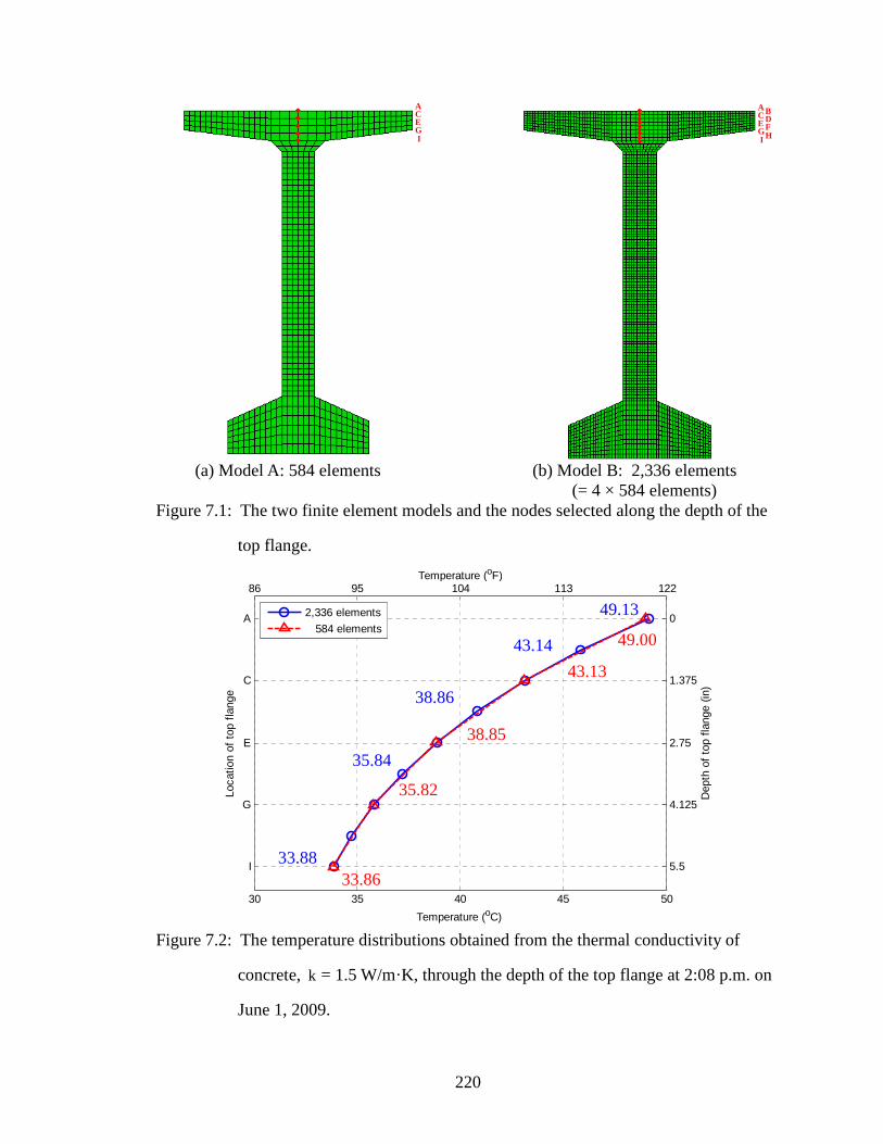
220

(a) Model A: 584 elements (b) Model B: 2,336 elements (= 4 × 584 elements) Figure 7.1: The two finite element models and the nodes selected along the depth of the

top flange.


concrete, k = 1.5 W/m·K, through the depth of the top flange at 2:08 p.m. on

June 1, 2009.

30 35 40 45 50

I

G

E

C

A

Temperature (oC)

Loca

tion

of t

op f

lang

e

2,336 elements

584 elements

86 95 104 113 122

5.5

4.125

2.75

1.375

0

Temperature (oF)

Dep

th o

f to

p fla

nge

(in)

49.00

43.13

38.85

33.86

35.82

49.13

43.14

38.86

35.84

33.88

A C E G I

A C E G I

B D F H

221



June 1, 2009.



June 1, 2009.

30 35 40 45 50

I

G

E

C

A

Temperature (oC)

Loca

tion

of t

op f

lang

e

2,336 elements

584 elements

86 95 104 113 122

5.5

4.125

2.75

1.375

0

Temperature (oF)

Dep

th o

f to

p fla

nge

(in)

30 35 40 45 50

I

G

E

C

A

Temperature (oC)

Loca

tion

of t

op f

lang

e

2,336 elements

584 elements

86 95 104 113 122

5.5

4.125

2.75

1.375

0

Temperature (oF)

Dep

th o

f to

p fla

nge

(in)

47.88

43.13

39.57

35.09

36.94

47.97

43.13

39.58

36.96

35.12

47.09

47.16

43.09

40.03

37.70

35.98

43.08

40.02

37.69

35.96

222

(Units: °C)

Thermal Conductivity, (W/m·K)

Locations

A C E G I

1.5 49.00 43.13 38.85 35.82 33.86 (0 %) (0 %) (0 %) (0 %) (0 %)

2.0 47.88 43.13 39.57 36.94 35.09

(-2.3%) (0 %) (1.9 %) (3.1 %) (3.6 %)

2.5 47.09 43.08 40.02 37.69 35.96

(-3.9%) (-0.1%) (3.0 %) (5.2 %) (6.2 %)



depth of the top flange at 2:08 p.m. on June 1, 2009.

₠ of web

30 35 40 45 50

I

G

E

C

A

Temperature (oC)

k=1.5 W/m.K

k=2.0 W/m.K

k=2.5 W/m.K

86 95 104 113 122

0

1.375

2.75

4.125

5.5

Temperature (oF)

Dep

th o

f to

p fla

nge

(in)

223

(Units: °C)

Thermal Conductivity,

(W/m·K)

Locations

A B C D E F G

1.5 49.00 35.82 31.84 31.48 30.41 29.44 33.25 (0 %) (0 %) (0 %) (0 %) (0 %) (0 %) (0 %)

2.0 47.88 36.94 32.63 31.87 30.84 30.13 33.04

(-2.3%) (3.1%) (2.5%) (1.3%) (1.4%) (2.4%) (-0.6%)

2.5 47.09 37.69 33.27 32.12 31.15 30.67 33.00

(-3.9%) (5.2%) (4.5%) (2.0%) (2.4%) (4.2%) (-0.8%)



depth of the BT-63 girder at 2:08 p.m. on June 1, 2009.

A

B

C

D

E

F

G 30 35 40 45 50

G

F

E

D

C

BA

Temperature (oC)

k=1.5 W/m.K

k=2.0 W/m.K

k=2.5 W/m.K

86 95 104 113 122

0

6

12.5

33

53.5

6063

Temperature (oF)

Dep

th o

f the

BT

-63

gird

er (

in)

224

Furthermore, Figures 7.7 to 7.9 show temperature contours obtained at 12:23,

2:42, and 4:27 p.m. on June 1, 2009 from the thermal conductivity of 1.5, 2.0, and 2.5

W/m·K, respectively. The figures represent the main heat flow from the top surface to

the bottom flange of the girder due to the solar heating of the top surface over time. The

bottom flange exhibits both vertical and transverse heat flows caused by solar radiation

incident on the south top and vertical surfaces of the bottom flange. Figures 7.7 to 7.9

also exhibit heat transfer from the highest temperature contours at 12:23 p.m. With

increases in thermal conductivity, the temperature contours showed rapid heat flow from

the top surface of the girder which resulted in temperature decreases on the top surface

and temperature increases inside the girder. The temperature differences between the

thermal conductivity of 1.5, 2.0, and 2.5 W/m·K were less than about 2°C (3.5°F).

225

(a) Temperature contour at 12:23 PM (b) Temperature contour at 2:42 PM (c) Temperature contour at 4:27 PM

Figure 7.7: Variations in temperature contours over the cross-section of the BT-63 girder obtained using k = 1.5 W/m·K for the

thermal conductivity.

226


Figure 7.8: Variations in temperature contours over the cross-section of the BT-63 girder obtained usingk = 2.0 W/m·K for the


227


Figure 7.9: Variations in temperature contours over the cross-section of the BT-63 girder obtained using k = 2.5 W/m·K for the


228

7.3.2 Specific Heat of Concrete

In addition to the thermal conductivity of concrete, the specific heat of concrete

also affects temperature distributions in prestressed concrete bridge girders. According to

the literature review, the specific heat of concrete ranges from approximately 800 to

1,200 J/kg·K. The values of the specific heat chosen in this study are 800, 1000, and

1200 J/kg·K. The thermal conductivity and the solar absorptivity of concrete maintained

the values of 1.5 W/m·K and 0.5, respectively, during the analysis.

Figure 7.10 shows the temperature distributions obtained from the heat transfer

analysis of the three specific heat values, 800, 1,000, and 1,200 J/kg·K. In addition,

Figure 7.11 presents the vertical temperature distributions along the depth of the BT-63

girder with increases in the specific heat of concrete at 2:08 p.m. when high girder

temperatures were measured. Since specific heat capacity is the amount of heat energy

required to raise the temperature by one degree per unit mass, the temperatures decreased

with increases in the specific heat of concrete. Indeed, as the specific heat of concrete

increased from 800 to 1,200 J/kg·K, the girder temperatures decreased by approximately

1°C (1.8°F) to 4°C (7.2°F), or 4 to 10%.

229

(Units: °C)

Specific Heat, (J/kg·K)

Locations

A C E G I

800 50.64 45.17 41.11 38.12 36.05 (0 %) (0 %) (0 %) (0 %) (0 %)

1,000 49.00 43.13 38.85 35.82 33.86

(-3.2%) (-4.5 %) (-5.5 %) (-6.0 %) (-6.1 %)

1,200 47.75 41.60 37.17 34.16 32.32

(-5.7%) (-7.9%) (-9.6 %) (-10.4 %) (-10.3 %)


heat of concrete, c = 800, 1000, and 1200 J/kg, through the depth of the top

flange at 2:08 p.m. on June 1, 2009.

₠ of web 30 35 40 45 50 55

I

G

E

C

A

Temperature (oC)

c=800 J/kg.K

C=1000 J/kg.K

c=1200 J/kg.K

86 95 104 113 122 131

0

1.345

2.75

4.125

5.5

Temperature (oF)

Dep

th o

f top

flan

ge (

in)

230

(Units: °C)

Specific Heat, (J/kg·K)

Locations

A B C D E F G

800 50.64 38.12 33.42 32.59 31.36 30.54 34.04 (0 %) (0 %) (0 %) (0 %) (0 %) (0 %) (0 %)

1,000 49.00 35.82 31.84 31.48 30.41 29.44 33.25

(-3.2%) (-6.0%) (-4.7%) (-3.4%) (-3.0%) (-3.6%) (-2.3%)

1,200 47.75 34.16 30.79 30.66 29.79 28.82 32.77

(-5.7%) (-10.4%) (-7.9%) (-5.9%) (-5.0%) (-5.6%) (-3.7%)


heat of concrete, c = 800, 1000, and 1200 J/kg, through the depth of the BT-

63 girder at 2:08 p.m. on June 1, 2009.

A

B

C

D

E

F

G 30 35 40 45 50 55

G

F

E

D

C

BA

Temperature (oC)

c=800 J/kg.K

c=1000 J/kg.K

c=1200 J/kg.K

86 95 104 113 122 131

0

6

12.5

33

53.5

6063

Temperature (oF)

Dep

th o

f the

BT

-63

gird

er (

in)

231

7.3.3 Solar Absorptivity of Concrete

For concrete exposed to the sun, the solar absorptivity of concrete is the factor

used to determine the amount of solar heat flux absorbed by the concrete surface. The

values of concrete solar absorptivity used in several studies in the literature are in the

range of 0.5 to 0.8 as described in Table 7.2. Thus, with respect to the values 0.5, 0.6,

0.7, and 0.8 of concrete solar absorptivity, variations in temperature distributions along

the depth of the BT-63 girder were evaluated. During the analysis, the other thermal

properties of concrete maintained constant: 1.5 W/m·K of thermal conductivity and

1,000 J/kg·K of specific heat.

Figures 7.12 and 7.13 show the temperature distributions obtained from the four

values of concrete solar absorptivity along the depth of the top flange and along the depth

of the girder, respectively. As solar absorptivity increased by 0.1, the temperatures on

the top surface increased by about 8%, or 4°C (7.2°F). The temperature increased by 5%,

or 1.8°C (3.2°F), in the middle of the top flange (location B); 2.5%, or 0.8°C (1.4°F), in

the middle of the web (location D); and 1.2%, or 0.4°C (0.7°F), in the middle of the

bottom flange (location F) with increases in solar absorptivity by 0.1. The bottom

surface, affected by solar radiation reflection or heat radiating from the ground, showed

an increase of 3%, or 1.0°C (1.8°F), with an increase of 0.1 in the solar absorptivity.

232

(Units: °C)

Solar Absorptivity Locations

A C E G I

0.5 49.00 43.13 38.85 35.82 33.86 (0 %) (0 %) (0 %) (0 %) (0 %)

0.6 52.93 46.14 41.15 37.61 35.29 (8.0%) (7.0 %) (5.9%) (5.0%) (4.2%)

0.7 56.83 49.12 43.44 39.39 36.72

(16.0%) (13.9%) (11.8%) (10.0%) (8.4%)

0.8 60.71 52.08 45.72 41.16 38.14

(23.9%) (20.8%) (17.7%) (14.9%) (12.6%)



top flange at 2:08 p.m. on June 1, 2009.

₠ of web 30 35 40 45 50 55 60 65

I

G

E

C

A

Temperature (oC)

a=0.5

a=0.6a=0.7

a=0.8

86 95 104 113 122 131 140 149

0

1.345

2.75

4.125

5.5

Temperature (oF)

Dep

th o

f to

p fla

nge

(in)

233

(Units: °C)

Solar Absorptivity

Locations

A B C D E F G

0.5 49.00 35.82 31.84 31.48 30.41 29.44 33.25 (0 %) (0 %) (0 %) (0 %) (0 %) (0 %) (0 %)

0.6 52.93 37.61 32.85 32.28 30.83 29.80 34.24 (8.0%) (5.0%) (3.2%) (2.5%) (1.4%) (1.2%) (3.0%)

0.7 56.83 39.39 33.86 33.08 31.25 30.16 35.23

(16.0%) (10.0%) (6.3%) (5.1%) (2.8%) (2.4%) (6.0%)

0.8 60.71 41.16 34.87 33.88 31.66 30.52 36.21

(23.9%) (14.9%) (9.5%) (7.6%) (4.1%) (3.7%) (8.9%)



BT-63 girder at 2:08 p.m. on June 1, 2009.

A

B

C

D

E

F

G 30 35 40 45 50 55 60 65

G

F

E

D

C

BA

Temperature (oC)

86 95 104 113 122 131 140 149

0

6

12.5

33

53.5

6063

Temperature (oF)

Dep

th o

f th

e B

T-6

3 gi

rder

(in

)

a=0.5

a=0.6

a=0.7

a=0.8

234

7.3.4 The Rate of Temperature Changes with the Thermal Properties of Concrete

Based on the temperature distributions at 2:08 p.m., Figure 7.14 shows changes in

the temperature distributions along the depth of the girder with changes in the thermal

properties of concrete. The reference values of the thermal properties of concrete were

1.5 W/m·K for thermal conductivity, 1,000 J/kg·K for specific heat, and 0.5 for solar

absorptivity. For example, for a parametric study on thermal conductivity, the specific

heat and the solar absorptivity of concrete were constants of 1,000 J/kg·K and 0.5,

respectively, during the analysis. As discussed previously, with increases in thermal

conductivity, Figure 7.14 shows temperature decreased on the surfaces of the girder due

to rapid heat absorption on the surface but temperature increased inside the girder. For

the specific heat of concrete, the girder temperatures decreased with increases in the

specific heat. Figure 7.14 also presents increases in the temperatures with increases in

the solar absorptivity.

Furthermore, this study evaluated the rate of temperature increases or decreases

with changes in the thermal properties of concrete. Figure 7.15 shows the percentage

change of the temperatures in the middle of the top flange, the web, and the bottom

flange. The percentage change of the temperatures with increases in the thermal

properties of concrete is summarized in Table 7.3. In the web of the girder, as the thermal

conductivity and the solar absorptivity of concrete increased by units of 1 W/m·K and

0.1, respectively, the temperatures increased about 2% (1°C). On the other hand, with

increases in the specific heat of concrete by a unit of 100 J/kg·K, the temperatures

decreased about 2% (1°C). Therefore, in the heat transfer analysis of prestressed

concrete bridge girders subjected to environmental thermal effects, the influences of the

thermal properties of concrete would be minimal when thermal properties are within

reasonable ranges.

235

Figure 7.14: Changes in the temperature distributions through the depth of the BT-63

girder with changes in the thermal properties of concrete.

-6 -3 0 3 6

web

web

Temperature Change (%)

k = 1.5 W/m.K

k = 2.0 W/m.K

k = 2.5 W/m.K

-2 -1 0 1 2

web

web

Temperature Change (oC)

k = 1.5 W/m.K

k = 2.0 W/m.K

k = 2.5 W/m.K

-12 -9 -6 -3 0

web

web


c = 800 J/kg.K

c = 1000 J/kg.K

c = 1200 J/kg.K

-5 -4 -3 -2 -1 0

web

web


c = 800 J/kg.K

c = 1000 J/kg.K

c = 1200 J/kg.K

0 5 10 15 20 25

web

web


a = 0.5

a = 0.6a = 0.7a = 0.8

0 2 4 6 8 10 12

web

web


a = 0.5

a = 0.6a = 0.7

a = 0.8

236

Figure 7.15: The percentage change of the girder temperatures with increases in the

thermal properties of concrete.

1.5 2 2.5

0

1.5

3

4.5

6

Thermal Conductivity of Concrete (W/m.K)

Incr

ease

(%

)

Middle of Top Flange

Middle of Web

Middle of Bottom Flange

1.5 2 2.5

0

0.5

1

1.5

2

Thermal Conductivity of Concrete (W/m.K)

Incr

ease

(o C)


Middle of Web


800 1000 1200

-10

-8

-6

-4

-2

0

Specific Heat of Concrete (J/kg.K)

Incr

ease

(%

)


Middle of Web


800 1000 1200

-4

-3.2

-2.4

-1.6

-0.8

0

Specific Heat of Concrete (J/kg.K)

Incr

ease

(o C)


Middle of Web


0.5 0.6 0.7 0.8

0

5

10

15

Solar Absorptivity of Concrete

Incr

ease

(%

)


Middle of WebMiddle of Bottom Flange

0.5 0.6 0.7 0.8

0

2

4

6

Solar Absorptivity of Concrete

Incr

ease

(o C)


Middle of WebMiddle of Bottom Flange

237

Table 7.3: The percentage change of the girder temperatures with changes in the thermal

properties of concrete.

Thermal Properties Change Rates of Properties

Percentage Change of Temperatures


Thermal Conductivity 1 W/m·K + 5% (+2°C) + 2% (+1°C) + 4% (+1.0°C)

Specific Heat 100 J/kg·K - 3% (-1°C) - 2% (-1°C) - 2% (-0.5°C)

Solar Absorptivity 0.1 + 5% (+2°C) + 3% (+1°C) + 3% (+0.5°C)

7.4 Thermal Movements with the Coefficient of Thermal Expansion (CTE)

Furthermore, to evaluate the influence of the CTE in the thermal behavior of

prestressed concrete bridge girders, the 3D thermal stress analyses were carried out on the

100-foot BT-63 girder with changes in the CTE from 6 to 12 × 10-6 / °C. The other

thermal properties of concrete maintained constant: 1.5 W/m·K for thermal conductivity,

1,000 J/kg·K, for specific heat, and 0.5 for solar absorptivity. The CTE of the

prestressing strands also remained constant at 12 × 10-6 / °C during the analysis. Since

the 3D thermal stress analysis consumes more time, this study used hourly temperature

fields obtained from extreme summer environmental conditions in Atlanta, Georgia

instead of measurements at five-minute intervals on June 1, 2009. The support boundary

conditions of elastomeric bearing pads were modeled as rigid vertical restraints as

described in Section 4.2.

Figures 7.16 and 7.17 show variations in the vertical and transverse thermal

movements at mid-span of the BT-63 girder for the CTE of 6, 9 and 12 × 10-6 / °C,

respectively. With increases in the CTE, the vertical and transverse thermal movements

proportionally increased. The maximum vertical movements were 0.21, 0.31, ad 0.42

inches at 3:00 p.m. in the CTE of 6, 9 and 12 × 10-6 / °C, respectively. The maximum

238

transverse thermal movements also linearly increased from 0.20 to 0.40 inches. Figure

7.18 exhibits the percentage change of the maximum vertical and transverse thermal

movements, which double for the CTE that doubles from 6 to 12 × 10-6 / °C. Thus, the

vertical and transverse thermal movements would change linearly in proportion to the

changes in the CTE. For the 100-foot BT-63 girder, the maximum vertical and transverse

thermal movements increase by approximately 0.03 inches (16%) with an increase by a

unit of 1 × 10-6 / °C from 6 × 10-6 / °C.

239

Figure 7.16: Variations in the vertical thermal movements at mid-span of the BT-63


10-6 / °C.

Figure 7.17: Variations in the transverse thermal movements at mid-span of the BT-63


10-6 / °C.

0 4 8 12 16 20 24-0.1

0

0.1

0.2

0.3

0.4

0.5

Time (hr)

Ver

tical

Dis

plac

emen

t (in

)

CTE = 6 x 10-6 / oC

CTE = 9 x 10-6 / oC

CTE = 12 x 10-6 / oC

0 4 8 12 16 20 24-0.1

0

0.1

0.2

0.3

0.4

0.5

Time (hr)

Tra

nsve

rse

Dis

plac

emen

t (in

)

CTE = 6 x 10-6 / oC

CTE = 9 x 10-6 / oC

CTE = 12 x 10-6 / oC

240

(a) Maximum vertical thermal movements

(b) Maximum transverse thermal movements

Figure 7.18: The percentage change of the maximum vertical and transverse thermal

movements with increases in the coefficient of the thermal expansion of

concrete.

6 9 12

0

50

100

CTE (x 10-6 / oC)

Incr

ease

(%

)

6 9 12

0

0.1

0.2

CTE (x 10-6 / oC)

Incr

ease

(in

)

6 9 12

0

50

100

CTE (x 10-6 / oC)

Incr

ease

(%

)

6 9 12

0

0.1

0.2

CTE (x 10-6 / oC)

Incr

ease

(in

)

241

CHAPTER 8

CONCLUSIONS AND RECOMMENDATIONS

8.1 Conclusions

This study first investigated variations in vertical and transverse temperature

distributions in prestressed concrete bridge girders due to environmental effects. A two-

dimensional (2D) finite element heat transfer model was then developed which accounted

for heat conduction in the concrete girder, heat convection between the environment and

the girder surface, heat irradiation from the sun, and heat radiation to the surroundings.

Since most of weather stations provide only daily solar radiation incident on a horizontal

surface, the 2D heat transfer analysis included the calculation of variations in solar

radiation with respect to the time of day on each surface of the girder according to the

location and geometry of the girder, the position of the sun, and the shadow on the web

and the bottom flange of the girder. The magnitudes and the variations of the predicted

temperatures were in very good agreement with experimental measurements performed

from April 2009 to March 2010.

Based on the relationships between environmental conditions and largest vertical

and transverse temperature distributions, seasonal extremes in environmental conditions

were determined from the 30-year (from 1961 to 1990) monthly data of the National

Solar Radiation Data Base, NSRDB, and the National Climatic Data Center, NCDC. The

developed 2D heat transfer model was then employed to determine seasonal extremes in

vertical and transverse temperature distributions and gradients for four selected

AASHTO-PCI standard girder sections. The influence of girder orientations on the

temperature distributions of the girders was also evaluated. The maximum vertical

temperature differentials were found in the summer in an east-west orientation, and the

242

maximum transverse temperature differentials were found in the winter in an east-west

orientation. Among the four AASHTO-PCI sections, the deeper and wider sections of

Type-V and BT-63 girders exhibited the largest vertical and transverse temperature

differentials.

For thermal gradients to be used in the design of prestressed concrete I-girders, a

revised vertical thermal gradient was first proposed. Figure 8.1 compares the vertical

thermal gradients proposed by the current study with the vertical thermal gradients in the

AASHTO specifications (1989, 2007) for Atlanta, Georgia. For a simply supported 100-

foot long BT-63 girder, the vertical thermal movement calculated using the proposed

vertical thermal gradient was approximately 40% higher than the vertical movement

calculated using the gradient in the AASHTO specifications.

The stability of the prestressed concrete girders largely depends on transverse

movements in the girder. However, the AASHTO specifications (1989, 2007) do not

provide any transverse thermal gradients. Therefore, this study also proposed transverse

thermal gradients for the top flange, web, and bottom flange of prestressed concrete I-

girders, as shown in Figure 8.2. The proposed vertical and transverse thermal gradients

were provided in terms of the locations of the top flange, the web, and the bottom flange

of the girders for the easy application to various I-shape girders.

The maximum vertical and transverse temperature differentials were evaluated at

eight cities in the United States. The eight cities were selected from the 30-year (from

1961 to 1990) monthly NSRDB and NCDC data based on extreme environmental

conditions such as the highest daily solar radiation, the highest record daily maximum

temperature, and the largest daily temperature variance: Alamosa, CO; Phoenix, AZ;

Medford, OR; Atlanta, GA; Brownsville, TX; Caribou, ME; Hilo, HI; Annette, AK.

243

Figure 8.1: The vertical thermal gradients of prestressed concrete bridge I-girders in Atlanta,

Georgia proposed by the current study and given in the AASHTO specifications

(1989, 2007).


Figure 8.2: The transverse thermal gradients of prestressed concrete bridge I-girders in

Atlanta, Georgia proposed by the current study (Not to Scale).

Bbot Bbot Bbot

Bbot = 1/4 × width of bottom flange

Bweb = 1/2 × width of web Btop = 1/4× width of top flange

T1= 20°C (36°F)

T2=1/4 × T1

Btop Btop

T1 = 16°C (29°F) T1 = 26°C (47°F)

Bweb Bweb

T2=1/4 × T1

T2=4/9 × T1

T3=1/9 × T1

T1 = 27°C (49°F)

T2 = 5°C (9°F)

Top flange

Bottom flange

Girder Depth

T3 ≤ 3°C (5°F)

Web

23°C (41°F)

AASHTO (2007)

AASHTO (1989)

244

The maximum girder temperatures were then transferred to the three-dimensional

(3D) finite element model of a 100-foot long BT-63 girder located in Atlanta with a

constant temperature variation along the length of the girder. The 3D thermal response

analysis considered in this study was composed of two sequential analyses; the first 3D

static analysis with a simply supported boundary condition and the second 3D thermal

stress analysis with elastomeric bearing pads. The bearing pads were modeled as

nonlinear springs with the effective vertical stiffness of the bearing pads. The analyses of

the girder did not exhibit any instability of the girder due to the combined effects of the

self-weight and temperature without any initial sweep or support rotation.

Since thermal effects are combined with fabrication and construction errors prior

to the placement of cross bracing and the deck slab, a 3D finite element sequential

analysis procedure was developed which accounted for the changes in the geometry and

stress state of the girder during construction and erection. This analysis included

geometric nonlinear behavior of the girder and the nonlinear behavior of the elastomeric

bearing pads. For the 100-foot BT-63 girder, the analyses indicated a possible instability

of the girder due to the combination of thermal effects with 4.5 inches of initial sweep

and a 5 degree support slope.

This study also developed a beam model with artificial end moments to calculate

the vertical and transverse thermal deformations induced by nonlinear temperature

distributions for simply supported girders. The end moments which cause vertical

deformations are obtained from a vertical temperature gradient along the depth of the

cross-section. The end moments which cause transverse deformations are defined as the

sum of three transverse temperature gradients of the top flange, the middle of the web,

and the bottom flange because the transverse temperature gradients vary from the top to

the bottom flanges. Compared with the results from the 3D finite element analysis, the

245

beam vertical and transverse movements were within 0.03 inches (6%). This study also

developed simplified equations for calculating the maximum vertical and transverse

thermal movements in terms of the span length of the girders for four selected AASHTO-

PCI standard girders; Type-I, Type-IV, Type-V, and BT-63 girders.

8.2 Recommendations for Future Studies

The current experimental and analytical investigations were carried out on a BT-

63 prestressed girder to determine variations in environmental conditions and girder

temperatures. To provide more generalized conclusions toward design recommendations

in the future, both experimental and analytical investigations are recommended for other

prestressed concrete girders from the construction stages until service load conditions.

The primary measurements and investigations are described below:

(1) A survey of geometry sweep and support imperfections present in newly

constructed girders.

(2) Development of criterion for initial slope imperfections

(3) Development of criterion for bracing requirements.

(4) Since the global stability behavior of prestressed concrete bridge girders are

largely affected by the behavior of elastomeric bearing pads, experimental and

analytical studies are also required to obtain the effective vertical and horizontal

stiffness of the bearing pads. Furthermore, the development of the three-

dimensional and simplified beam models are recommended for evaluating the

influences of the bearing pads on the behavior of the bridge systems under various

environmental and loading conditions.

246

APPENDIX A

A MODEL OF TRANSVERSE TEMPERATURE DISTRIBUTION

For the vertical temperature distribution through the depth of a concrete

superstructure, Priestley (1976) proposed a fifth-order temperature decrease from a

maximum temperature at the concrete top surface. The Priestley fifth-order model was a

basis of the current design specifications in many countries such as New Zealand, North

America, and England. However, no model has been suggested for the shape of

transverse temperature distributions in the concrete superstructure. The temperatures

along the transverse direction of a concrete bridge section are induced by the heating of

the vertical surface due to solar radiation and also affected by the vertical heat flow.

Thus, in order to describe the gradual decrease from the highest temperature in the

transverse direction, this study proposed a second-order model shown in Figure A.1. The

temperature ( )T x , shown in Figure A.1, is calculated using the following second-order

equation:

2( ) = ( / )sT x T x L (A.1)

in which ( ) T x = the temperature at a distance of x,

sT = the surface temperature,

x = the distance from the surface, and

L = the length from the surface to zero temperature.

247

Figure A.1: A model of the transverse temperature distribution.

For November 15, 2009, on which girder temperatures at thermocouple location 9

and 10 were missed due to a poor connection to data-logging system, the proposed

second-order model was used to extrapolate the missing temperatures from the surface

temperature (thermocouple 14) and the minimum temperature (thermocouple 11).

Compared with the temperatures obtained from finite-element heat transfer analysis,

those calculated by Equation (A.1) showed average absolute errors of 0.6°C (1.1°F) and

1.3°C (2.4°F) at the locations of the thermocouples 9 and 10, respectively. The maximum

difference between the temperatures obtained from the heat transfer analysis and the

Equation (A.1) was 3.3°C (5.8°F) at the thermocouple 9 and 2.6°C (4.7°F) at the

thermocouple 10.

Furthermore, this study compared maximum transverse temperature distributions

measured across the bottom flange (including the extrapolated temperatures at the

thermocouples 9 and 10) with those obtained from the finite element heat transfer

analysis. Figure A.2 shows the measured and predicted transverse temperature

distributions in the bottom flange on November 15, 2009. The magnitudes and shapes of

the transverse temperature distribution from the measurements agree well with the results

of the heat transfer analysis. The temperatures extrapolated using Equation (A.1) differed

Ts

L

T(x) x

248

from the results of the heat transfer analysis by only 0.2°C (0.4°F) and 0.7°C (1.3°F) at

the thermocouple location 9 and 10, respectively.


Heat Transfer Analysis, °C (°F)

36.4 (97.5)

24.5 (76.1)

17.6 (63.7)

15.6 (60.1)

19.1 (66.5)

Second-Order Model, °C (°F)

35.3 b (95.6)

24.9 a (76.8)

17.4 a (63.3)

14.9 b (58.8)

17.3 (63.2)

Difference, °C (°F) 1.1 (1.9) 0.4 (0.7) 0.2 (0.4) 0.7 (1.3) 1.8 (3.3)

a The temperatures at the thermocouple location 10 and 9 were extrapolated

using the second-order equation.

b The temperatures at the thermocouple location 14 and 11 were the measured maximum and minimum temperatures, respectively, across the bottom flange.

Figure A.2: Predicted and measured maximum transverse temperature distributions at the

thermocouple location across the bottom flange on November 15, 2009.

14 10 9 11 15

10

20

30

40

Tem

pera

ture

(o C)

Thermocouple No. across bottom flange

50

68

86

104

Tem

pera

ture

(o F)

Heat Transfer Analysis

Second-Order Model

North South

249

APPENDIX B

CALCULATION OF SOLAR POSITION

The calculation of solar radiation incident on girder surfaces requires that the

relationship between a position on the earth’s surface and the position of the sunlight be

determined. Figure B.1 shows the position of P on the earth’s surface and the sun at one

time in the summer. Point P, which represents a location in the Northern Hemisphere, is

expressed as the latitude of ϕ. The declination angle, δ, is the angular position of the sun

at solar noon with respect to the plane of the equator. The value of the declination at any

time can be calculated from the following equation (Cooper, 1969):

284

23.45sin 360365

nδ + =

(B.1)

in which n is the day of the year. The hour angle, ω, defined as the angular displacement

of the sun due to the rotation of the earth on its axis at 15° per hour, is zero at solar noon,

negative before solar noon, and positive in the afternoon.

Figure B.1: A position on the earth’s surface in relation to the direction of the radiation at

one specific time in the summer.

Equator

P

O

N

Solar radiation

ω

δ ϕ

250

The direct solar radiation incoming on a plane can be described in terms of the

geometrical relationships between the plane oriented in a particular direction and the

solar radiation. The position of the sun and the location of the plane relative to the sun

are defined in Figure B.2, in which the solar and plane angles are as follows.

Zθ : the zenith angle, defined as the angle between the line overhead and the line to the

sun.

θ :the incident angle, defined as the angle between the beam radiation on a horizontal

plane and the surface normal.

sα : the solar altitude angle, defined as the angle between the beam radiation on the

horizontal plane and the line to the sun.

sγ : the solar azimuth, defined as the angle of the projection of the beam radiation on the

horizontal plane from the south, with zero due south, negative to the east, and

positive to the west.

γ : the surface azimuth, defined as the angle of the projection of the surface normal onto

the plane from the south, with zero due south, negative to the east, and positive to

the west.

β : the surface angle relative to the horizontal plane.

With the data of the position of the sun related to the plane, solar angles θz, θ, and sγ are

calculated by (Liu and Jordan, 1963)

cos sin sin cos cos cosZθ δ φ δ φ ω= + , and (B.2)

cos sin sin cos sin cos sin cos

cos cos cos cos cos sin sin cos cos

cos sin sin sin

θ δ φ β δ φ β γδ φ β ω δ φ β γ ωδ β γ ω

= −+ ++

(B.3)

251

1 cos sinsin

sinsz

δ ωγθ

− =

(B.4)

Figure B.2: The angles of the solar position and the slope of a plane oriented in any

particular position.

N

S E

Vertical Surface normal

sγγ

Solar radiation

sα

Zθ

θProjection of a ray of the sun onto the horizontal plane

Projection of the surface normal onto the horizontal plane

β

252

APPENDIX C

CALCULATION OF THERMAL MOVEMENTS

USING A BEAM MODEL

For the 100-foot long BT-63 girder, the proposed beam model was used to

calculate vertical and transverse thermal movements from hourly vertical and transverse

temperature gradients obtained from the 2D heat transfer analysis. The environmental

conditions involved in this study were extreme summer and winter environmental

conditions in Atlanta, Georgia, when the largest vertical and transverse temperature

gradients were respectively found. Figure C.1 show the largest vertical temperature

gradient along the depth of the girder in the summer, and Figure C.2 show the transverse

temperature gradients across the middle of top flange, web, and bottom flange of the

girder in the winter.

Figure C.1: The largest vertical temperature gradient of the BT-63 girder in the summer

in Atlanta, Georgia.

0 5 10 15 20 25

0

10.5

57.5

63

Temperature (oC)

Dep

th o

f th

e T

ype-

I se

ctio

n (in

)

0 9 18 27 36 45

Temperature (oF)

253


Figure C.2: The largest transverse temperature gradients of the BT-63 girder in the winter in Atlanta, Georgia.

0 21 42

0

5

10

15

20

25

Tem

pera

ture

(o C)


0 3 6Width of Web (in)

0 13 26Width of Bottom Flange (in)

0

9

18

27

36

45

Tem

pera

ture

(o F)

254

Figure C.3 illustrates the vertical temperature differential at a depth of y from the

center of the gravity of the cross-section. Therefore, the artificial end moment Mx

induced by the vertical temperature gradient can be obtained from the following equation:

� = ;[' ∙ � ∙ ∆�� ∙ $� ∙ ]& = ∑['= ∙ �= ∙ ∆��= ∙ $�= ∙ = ∙ ∆=] (C.1)

in which '> = the concrete modulus of elasticity at a depth yi,

�= = the coefficient of thermal expansion of concrete at a depth yi,

∆��= = the vertical temperature differential at a depth yi, and

$�= = the width of the girder section at a depth yi,

(a) Cross-section (b) Vertical temperature gradient

Figure C.3: The cross-section and vertical temperature gradient of the BT-63 girder.

For a simple span, the vertical deformation yδ at mid-span is then calculated by

2

8x

yx

M L

EIδ = (C.2)

c.g.

yi

b(yi)

c.g.

yi

∆T(yi)

x

255

in which ) is the moment of inertia of the cross-section with respect to the x-axis, and L

is the length of the girder.

Figure C.4 shows variations in the vertical thermal movements of the BT-63

girder calculated using the beam model from the hourly vertical temperature gradients in

the summer and the winter in Atlanta, Georgia. The maximum vertical thermal

movements were 0.54 inches at in the summer and 0.20 inches in the winter.


Figure C.4: Variation in the vertical thermal movements of the 100-foot BT-63 girder


Georgia.

Similarly, for the calculations of the transverse thermal movements, the artificial

end moment My is determined from the transverse temperature gradients in the middle of

the top flange, the web, and the bottom flange as shown in Figure C.5. The end moment

My calculated from these three transverse temperature gradients is as shown below:

2 4 6 8 10 12 14 16 18 20 22

0

0.1

0.2

0.3

0.4

0.5

0.6

Time (hr)

Ver

tical

Dis

plac

emen

t (in

)

2 4 6 8 10 12 14 16 18 20 22

0

0.1

0.2

0.3

0.4

0.5

0.6

Time (hr)

256

[ ( ) ( ) ]

[ ( ) ( ) ]

[ ( ) ( ]

)

y i i i i i itop flange

i i i i i iweb

i i i i i ibottom flange

M E T x h x x x

E T x h x x

d

dx

E T x h x x xd

α

α

α

= ⋅ ⋅ ⋅ ⋅ ⋅ +

⋅ ⋅ ⋅ ⋅ ⋅ +

⋅ ⋅ ⋅ ⋅ ⋅

∑

∑

∑

(C.3)

in which '= = the concrete modulus of elasticity at a width xi,

�= = the coefficient of thermal expansion of concrete at a width xi,

∆��+= = the transverse temperature differential at a width xi, and

ℎ�+= = the height of the girder section at a width xi,

(a) Cross-section (b) Transverse temperature gradients

Figure C.5: The cross-section and transverse temperature gradients of the BT-63 girder.

Like to the vertical thermal movement, the transverse deformation xδ is then

calculated using the end moment My:

c.g.

xi

h(xi)

y

x

x

x

Top flange

Bottom flange

Web

257

2

8y

xy

M L

EIδ = (C.4)

in which )* is the moment of inertia of the cross-section with respect to the y-axis, and L

is the length of the girder. The variations in the transverse thermal movements calculated

from the hourly transverse temperature gradients under extreme environmental conditions

in the summer and the winter in Atlanta, Georgia are shown in Figure C.6. The

calculated maximum transverse thermal movements were 0.39 inches in the summer and

0.81 inches in the winter.


Figure C.6: Variation in the transverse thermal movements of the 100-foot BT-63 girder


Georgia.

2 4 6 8 10 12 14 16 18 20 22

0

0.2

0.4

0.6

0.8

1

Time (hr)

Tra

nsve

rse

Dis

plac

emen

t (in

)

2 4 6 8 10 12 14 16 18 20 22

0

0.2

0.4

0.6

0.8

1

Time (hr)

258

REFERENCES

AASHTO. (1989). AASHTO Guide specifications: Thermal effects in concrete bridge superstructures. Washington, DC: American Association of State Highway and Transportation Officials.

AASHTO. (2007). AASHTO LRFD bridge design specifications: 2008 interim revisions (4th ed.). Washington, DC: American Association of State Highway and Transportation Officials.

AASHTO. (2004). AASHTO LRFD bridge construction specifications: 2006 and 2007 interim revisions (2nd ed.). Washington, DC: American Association of State Highway and Transportation Officials.

AASHTO. (1999). Guide specifications for design and construction of segmental concrete bridges (2nd ed.). Washington, DC: American Association of State Highway and Transportation Officials.

ABAQUS. (2008). Abaqus version 6.8. Providence, RI: Dassault Systems Simulia Corp.

ACI Committee 435. (1995). Control of Deflection in Concrete Structures. ACI Committee Report. Farmington Hills, MI: American Concrete Institute.

Anderson, B. (1977). Solar Energy: fundamentals in building design. New York: McGraw-Hill, Inc.

ASHRAE. (2005). ASHRAE Handbook of Fundamentals. Atlanta, GA: American Society of Heating, Refrigerating, and Air-Conditioning Engineers.

Barber, E. S. (1957). Calculation of Maximum Pavement Temperatures from Weather Reports. Highway Research Board Bulletin, 168, 1-8.

Barr, P. J., Stanton, J. J., & Eberhard, M. O. (2005, March-April). Effects of thermal variations on precast prestressed concrete bridge girders. Journal of Bridge Engineering, 10 (2), 186-194.

259

Branco, F.A. & Mendes, P.A. (1993, August). Thermal actions for concrete bridge design. Journal of Structural Engineering, 199 (9), 2313-2331.

Chapman, A. J. (1960). Heat transfer (2nd ed.). New York: Macmillan Company.

Churchward, A. & Sokai, Y. J. (1981). Prediction of temperatures in concrete bridges. Journal of Structural Engineering, 107 (11), 2163-2176.

CIBSE. (1985). CIBSE Guide H: Building control systems (1st ed.). Oxford, UK: Butterworth-Heinemann.

Clark, J. H. (1989). Evaluation of thermal stresses in a concrete box girder bridge. Doctoral dissertation, University of Washington.

Cooper, P. I. (1969). The absorption of solar radiation in solar stills. Solar Energy, 12 (3), 336.

Dilger, W. H., Ghali, A., & Cheung, M. S. (1981, November). Field Measurements of Muskwa River Bridge. Journal of Structural Division, 107 (11), 2147-2161.

Dilger, W. H., Ghali, A., Cheung, M. S., & Maes, M. A. (1983). Temperature stresses in composite box girder bridges. Journal of Structural Engineering, 109 (6), 1460-1478.

Duffie, J. A. & Beckman, W. A. (1980). Solar engineering of thermal processes. New York: John Wiley & Sons, Inc.

Elbadry, M. M. & Ghali, A. (1983, October). Temperature variation in concrete bridges. Journal of Structural Engineering, 109 (10), 2355-2374.

Elbadry, M. M. & Ghali, A. (1986, November-December). Thermal stresses and cracking of concrete bridges. Journal of the American Concrete Institute, 83 (6), 1001-1009.

Emanuel, J. H. & Hulsey, J. L. (1978). Temperature distributions in composite bridges. Journal of the Structural Division, 104 (1), 65-78.

260

Emerson, M. (1973). The calculation of the distribution of temperature in bridge (TRRL Report LR 561). Berkshire, UK: Transport and Road Research Laboratory.

Erbs, D. G., Klein, S. A., & Duffie, J. A. (1982). Estimation of the diffuse radiation fraction for hourly, daily and monthly-average global radiation. Solar Energy, 28 (4), 293-302.

FHWA. (2002). 2002 pavement design guide (FHWA-RD-00-129). McLean, VA: Federal Highway Administration.

FDOT. (1997). FDOT structures design guidelines. Tallahassee, FL: Florida Department of Transportation.

GDOT. (2005). GDOT bridge and structures design policy manual: revised July 2009. Atlanta, GA: Georgia Department of Transportation.

Ghali, A. & Elbadry, M. M. (1989, January-February). Serviceability design of continuous prestressed concrete structures. Journal of the Prestressed Concrete Institute, 34(1), 54-91.

Ghali, A., Favre, R., & Elbadry, M. (2002). Concrete structures: stresses and deformations (3rd ed.). London: Spon Press.

Gilland, J. A., & Dilger, W. H. (1997). Monitoring concrete temperature during construction of the confederation bridge. Canadian Journal of Civil Engineering, 24, 941-950.

Hirst, M. J. S. (1984). Thermal loading of concrete bridges. Canadian Journal of Civil Engineering, 11, 423-429.

Laszlo, G. & Imper, R. R. (1987, November-December). Handling and shipping of long span bridge beams. PCI Journal, 32 (6), 86-101.

Incropera, F. P. & Dewitt, D. P. (2002). Fundamentals of heat and mass transfer (5th ed.). Hoboken, NJ: John Wiley & Sons, Inc.

Jansen, T. J. (1985). Solar engineering technology. Englewood Cliffs, NJ: Prentice-Hall Inc.

261

Kennedy, J. B. & Soliman, M. H. (1987). Temperature distribution in composite bridges. Journal of Structural Engineering, 113 (3), 475-482.

Kreith, F. (1973). Principles of heat transfer. New York: Harper & Row.

Kreith, F. & Kreider J. F. (1978). Principles of solar engineering. Washington: Hemisphere Publishing Corp.

Kouremenos, D. A., Antonopoulos, K. A., & Doulgerakis, S. (1987). Direct and diffuse solar radiation correlations for tilted surfaces in Athens, Greece. Solar Energy, 38 (3), 203-217.

Kuehn, T. H., Ramsey, J. W., & Threlkeld, J. L. (1998). Thermal environmental engineering (3rd ed.). Upper Saddle River, NJ: Prentice-Hall Inc.

Leonhardt, F., Kolbe, G., & Peter, J. (1965, July). Temperaturunterschiede gefahrden spannbetonbrucke (Temperature differences endanger prestressed concrete bridge, translated into to English). Beton-undStahlbetonbau, 60 (7), 157-163. In German.

Li, D., Maes, M. A., & Dilger, W. H. (2004). Thermal design criteria for deep prestressed concrete girders based on the data from confederation bridge. Canadian Journal of Civil Engineering, 31, 813-825.

Liu, B. Y. H. & Jordan, R. C. (1960). The interrelationship and characteristic distribution of direct, diffuse, and total solar radiation. Solar Energy, 4 (1), 1-19.

Liu, B. Y. H. & Jordan, R. C. (1963). The long-term average performance of flat-plate solar energy collectors. Solar Energy, 7 (2), 53-74.

Marion, W. & Wilcox, S. (1991) Solar radiation data manual for flat-plate and concentrating collectors. Golden, Colorado: National Renewable Energy Laboratory

Mast, R. F. (1989, January-February). Lateral stability of long prestressed concrete beams – part 1. PCI Journal, 34 (1), 34-53.

262

Mast, R. F. (1993, January-February). Lateral stability of long prestressed concrete beams – part 2. PCI Journal, 38 (1), 70-83.

Mirambell, E., & Aguado, A. (1990, September). Temperature and stress distributions in concrete box girder bridges. Journal of Structural Engineering, 116 (9), 2388-2409.

Moorty, S., & Roeder, C. W. (1992, April). Temperature-dependent bridge movements. Journal of Structural Engineering, 118 (4), 1090-1105.

Neville, A. M. (1996). Properties of Concrete (4th ed.). New Jersey: John Wiley & Sons, Inc.

Oesterle, R. G., Sheehan, M. J., Lotfi, H. R., Corley, W. G., & Roller, J. J. (2007, November). Investigation of red mountain freeway bridge girder collapse (CTLGroup Project No. 262291). Final report to Arizona state department of transportation, CTLGroup.

PCI. (2003). PCI bridge design manual (2nd ed.). Chicago, IL: Precast/Prestressed Concrete Institute.

PCI. (2000). PCI tolerance manual for precast and prestressed concrete construction (1st ed.). Chicago, IL: Precast/Prestressed Concrete Institute.

Pisani, M. A. (2004, August). Non-linear strain distributions due to temperature effects in compact cross-sections. Engineering Structures, 26 (10), 1349-1363.

Priestley, J.N. (1976, September). Design Thermal Gradients for Concrete Bridges. New Zealand Engineering, 31 (9), 213-219.

Priestley, J.N. (1978, May). Design of concrete bridges for temperature gradients. ACI Journal, 75 (23), 209-217.

Roberts-Wollman, C.L., Breen, J.E., & Cawrse, J. (2002, May). Measurements of thermal gradients and their effects on segmental concrete bridge. Journal of Bridge Engineering, 7(3), 166-174.

263

Saetta, A., Scotta, R., & Vitaliani, R. (1995). Stress analysis of concrete structures subjected to variable thermal loads. Journal of Structural Engineering, 121 (3), 446-457.

Soliman, M. H. & Kennedy, J. B. (1986). Simplified method for estimating thermal stresses in composite bridges (Transportation Research Record 1072, p. 23-31). Washington, DC: National research council.

Suchinda, C. & Will, K. M. (1999, June). A temperature response measurement in fiber reinforced polymeric bridge decks. Proceedings of Sixth Annual International Conference on Composite Engineering. Orlando, FL.

Suchinda, C. (2000). Experimental and analytical investigation of the thermal behavior of a fiber reinforced polymeric bridge deck. Doctoral dissertation, Georgia Institute of Technology.

Threlkeld, J. L. (1970). Thermal environmental engineering, Englewood Cliff, NJ: Prentice-Hall Inc.

VanGreem, M.G., Gajda, J., & Dombrowski, K. (1997). Thermal properties of commercially available high-strength concretes. Cement, Concrete, and Aggregates, 19(1), 38-53.

Will, K. M. (1975). Analytical and experimental investigation of the thermal response of highway bridges. Doctoral dissertation, University of Texas at Austin.

Will, K. M., Johnson, C. P., & Matlock, H. (1977). Analytical and experimental investigation of the thermal response of highway bridges (Research Project 23-2). Interim report to Texas state department of highways and public transportation, University of Texas at Austin.

Williamson, P. J. (1967). Estimation of heat outputs for road heating installations (Road Research Laboratory Report 77). London, UK: Ministry of Transport.

Yazdani, N., Eddy, S. M., & Cai, C. S. (2000, May-June). Validation of AASHTO bearing stiffness for standard precast concrete bridge girders. ACI Structural Journal, 97 (3), 436-443.

264

Yazdani, N., Eddy, S. M., & Cai, C. S. (2000, August). Effect of bearing pads on precast prestressed concrete bridges. Journal of Bridge Engineering, 5 (3), 224-232.

Zuk, W. (1961, September). Thermal and Shrinkage Stresses in Composite Beams. ACI Journal, 58 (3), 327-340.

Zuk, W. (1965). Thermal Behavior of Composite Bridges—Insulated and Uninsulated. Highway Research Record 76, 231-253.

265

VITA

JONG-HAN LEE

Jong-Han Lee earned his B.S. and M.S. degrees in Civil Engineering in Korea.

He conducted research involving structural dynamics and earthquake analysis associated

with structure-soil-fluid interactions, as well as nondestructive evaluation in civil

engineering structures. He earned his Ph.D. degree in 2010 in Civil Engineering at the

Georgia Institute of Technology in Atlanta, Georgia. During his Ph.D. studies, he focused

on the structural stability of reinforced and prestressed concrete bridge systems. This

research involved the nonlinear behavior of the structure, the investigation of

experimental and analytical methods, and the application of these methods to design.

experimental and analytical investigations of the thermal

Documents

Transcript of experimental and analytical investigations of the thermal