Mathematical and Computer Modelling 52 (2010) 346–354

Contents lists available at ScienceDirect

Mathematical and Computer Modelling

journal homepage: www.elsevier.com/locate/mcm

Existence results and numerical simulation of magnetohydrodynamicviscous flow over a shrinking sheet with suctionF. Talay Akyildiz a,∗, Dennis A. Siginer ba Department of Mathematics, Petroleum Institute, P.O. Box 2533, Abu Dhabi, United Arab Emiratesb Departments of Mechanical Engineering and Mathematics, Petroleum Institute, P.O. Box 2533, Abu Dhabi, United Arab Emirates

a r t i c l e i n f o

Article history:Received 29 November 2009Received in revised form 22 February 2010Accepted 24 February 2010

Keywords:Boundary layerMHD flowSchauder theoryGalerkin–Legendre spectral methodDomain truncation

a b s t r a c t

This paper presents an analysis and a semi-analytical study of the boundary value problemresulting from a self-similar transformation of the partial differential equations governingthe magnetohydrodynamic (MHD) viscous flow due to a shrinking sheet with suction.Existence of a solution is shown using the fixed point argument and the boundary valueproblem is solved. Galerkin–Legendre spectral method with domain truncation is used toobtain approximate analytical solutions. The approximate solutions computed confirm thetheoretical analysis.

© 2010 Elsevier Ltd. All rights reserved.

1. Introduction

The flow induced by a moving boundary is important in the extrusion processes in plastic and metal industries [1–3].The pioneering work investigating the boundary layer flow on a continuously stretching surface with a constant speed wasexplored out by Sakiadis [4,5]. His work was further verified experimentally by Tsou et al. [6] and the boundary conditionson the surface were generalized by other researchers [7–14]. These investigations look into flow problems over stretchingsheets. The literature on flows over shrinking sheets is very scarce. The unsteady flow problem over a shrinking sheet wasfirst considered by Wang [15]. The existence and non-uniqueness of steady viscous hydrodynamic flow due to a shrinkingsheet for a specific value of the suction parameter were shown by Miklavcic and Wang [16]. The magnetohydrodynamic(MHD) viscous flow over a shrinking sheet was considered by Sajid and Hayat [17] who solved the problem by using thehomotopy analysis method (HAM). The exact analytical solution of the same problem for special values of a parameterembedded in the nonlinear differential equation was obtained by Fang and Zhang [18].The magnetohydrodynamic (MHD) viscous flow problem over a shrinking sheet considered by Sajid and Hayat [17] and

Noor et al. [19] is taken up in this paper and the existence of the solution is shown for the first time, specifically the existenceof the governing third order nonlinear differential equation is proven, followed by an application of the Galerkin–Legendrespectral method with domain truncation not considered in [17,19] to obtain an approximate analytical solution of theproblem under consideration.Despite the importance and frequent occurrence of non-Newtonian behavior in technological applications no work

concerning the existence of the solution of the governing field equations has been reported in the literature concerningthe flow of a non-Newtonian fluid over a permeable or non-porous shrinking surface. The existence of the solution for theflow of an upper convected Maxwell fluid over a shrinking sheet is under consideration by the present authors.

∗ Corresponding author.E-mail addresses: fakyildiz@pi.ac.ae (F.T. Akyildiz), dsiginer@pi.ac.ae (D.A. Siginer).

0895-7177/$ – see front matter© 2010 Elsevier Ltd. All rights reserved.doi:10.1016/j.mcm.2010.02.049

F.T. Akyildiz, D.A. Siginer / Mathematical and Computer Modelling 52 (2010) 346–354 347

2. Mathematical formulation

In Cartesian coordinates the continuity and momentum equations for MHD viscous flow are

∂u∂x+∂v

∂y+∂w

∂z= 0, (2.1)

u∂u∂x+ v

∂u∂y+ w

∂u∂z= −

1ρ

∂p∂x+ v

(∂2u∂x2+∂2u∂y2+∂2u∂z2

)−σB20ρu, (2.2)

u∂v

∂x+ v

∂v

∂y+ w

∂v

∂z= −

1ρ

∂p∂y+ v

(∂2v

∂x2+∂2v

∂y2+∂2v

∂z2

)−σB20ρv, (2.3)

u∂w

∂x+ v

∂w

∂y+ w

∂w

∂z= −

1ρ

∂p∂z+ v

(∂2w

∂x2+∂2w

∂y2+∂2w

∂z2

), (2.4)

where v = µ/ρ and σ are the kinematic viscosity and the electrical conductivity, respectively. The magnetic field B0 isapplied in the z-direction and the inducedmagnetic field is neglected. Eqs. (2.1)–(2.4) imply zero electric field influence andsmall magnetic Reynolds number. The boundary conditions on the shrinking surface at z = 0 are,

u = −ax, v = −a(m− 1)y, w = −W (2.5)where a > 0 andW are the shrinking constant and the suction velocity, respectively. The parameterm assumes the valuesof 1 and 2, when the sheet shrinks in the x direction alone and when the sheet shrinkage is axisymmetric, respectively. Farfrom the sheet the fluid has no lateral velocities and the pressure is uniform. The following similarity transform is used,

u = axf ′(η), v = a(m− 1)yf ′(η), w = −√avmf (η), (2.6)

where η = z√a/v. Eq. (2.1) is automatically satisfied, Eq. (2.4) becomes,

pρ= vwz −

w2

2+ constant (2.7)

and (2.2), (2.3) are reduced to the following nonlinear ordinary differential equation

f ′′′ −M2f ′ +mff ′′ − (f ′)2 = 0, (2.8)with boundary conditions

f ′(0) = −1, f (0) = s, f ′(∞) = 0, (2.9)where s = W/m

√av andM2 = σB20/ρa. Changing variables (η) = s+ ψ(η), (2.8) and (2.9) can be rewritten as

ψ ′′′ −M2ψ ′ +mψψ ′′ − (ψ ′)2 +mψ ′′ = 0,ψ ′(0) = −1, ψ(0) = 0, ψ ′(∞) = 0.

. (2.10)

Exact analytical solutions of (2.8) are possible for special values of m and s are given in [16,18]. However the existence ofthe solution of (2.10) for positive values ofm has never been studied and the solution has not been obtained before.

Existence

3. Introduction

A change of variables g(η) = ψ ′(η) transforms (2.10) into,

g ′′ −M2g +m(∫ η

0g(τ )dτ

)g ′ − g2 +mg ′ = 0, 0 < η <∞,

g(0) = −1, and limη→∞

g(η) = 0.

. (3.1)

We now focus on the problem

g ′′ −M2g +m(∫ η

0g(τ )dτ

)g ′ − g2 +mg ′ = 0, 0 < η < R,

g(0) = −1, and g(R) = 0,

(3.2)

where R is an arbitrary but fixed positive number. For problem (3.2), we shall define a mapping via a linear second orderproblem whose fixed points constitute a solution to problem (3.2). Then application of the Schauder fixed point theorem issummarized in the following statement.

Theorem 3.1. For each positive m, there exists non-positive classical solution g of problem (3.2) satisfying the inequality−1 < g< 0 on 0 < η < R.

348 F.T. Akyildiz, D.A. Siginer / Mathematical and Computer Modelling 52 (2010) 346–354

Proof. See the following analysis.Define the continuous functions on the interval 0 ≤ η ≤ Rwhich are negative in 0 < η < R as

S = φ ∈ C[0, R] | φ(η) < 0, 0 < η < R. (3.3)

C[0, R] is the Banach space of continuous functions on 0 ≤ η ≤ Rwith the norm

‖φ‖ = max0≤η≤R

|φ(η)|. (3.4)

Now consider the mapping T : S → S with Tφ defined as the solution g of

g ′′ −M2φ +m(∫ η

0φ(τ)dτ

)g ′ − φg +mg ′ = 0, 0 < η < R,

g(0) = −1, and g(R) = 0.

. (3.5)

This is a linear second order boundary value problem with continuous coefficients, hence, there exists a unique classicalsolution g for each φ ∈ S and the mapping T is well defined. As a first estimate we demonstrate the following.

Proposition 3.1. For each φ ∈ S, g = Tφ, satisfies

− 1 ≤ g(η) ≤ 0, 0 ≤ η ≤ R. (3.6)

Proof. First assume that g < −1 and g + M2 < 0 at some point η in 0 ≤ η ≤ R. Then g would have a negative maximumin 0 < η < R at say ηl. Hence, at ηl

0 ≥ g ′′(ηl)+m(∫ ηl

0φ(τ)dτ

)g ′(ηl)+mg ′ = φ(ηl)(g +M2) > 0 (3.7)

which contradicts (3.2), hence g(η) ≥ −1. Similarly, we can show that (3.5) is satisfied with the inequalities reversed at apositive minimum.

Proposition 3.2. Let g be a classical solution of (3.2) such that −1 ≤ g(η) ≤ 0 for 0 < η ≤ R. If M2g(η)+ g(η)2 ≤ 0, theng ′(η) ≥ 0 for all 0 < η ≤ R.

Proof. Since g(0) = −1, g(R) = 0 and −1 ≤ g(η) ≤ 0, it follows from elementary calculus that g ′(0) ≥ 0 and g ′(R) ≥ 0for all 0 < η ≤ R. Now set

A(η) = em∫ η0∫ z0 g(s)dsdz+m

∫ η0 g(s)ds.

Clearly A(η) ≥ 1 for all η ≥ 0, and (3.2) can be written as

(A(η)g ′(η))′ = A(η)(M2g + g2) ≤ 0. (3.8)

It then follows that A(η)g ′(η) is decreasing and

A(η)g ′(η) ≥ A(R)g ′(R) ≥ 0. (3.9)

Since A(η) > 0 for all η ≥ 0 and g ′(R) ≥ 0, it follows that g ′(η) ≥ 0 for all 0 < η < R.

Proposition 3.3. For each solution of (3.2) if (g ′(R) − g ′(0)) ≤ 0 and bounded,∫ R0 g(s)ds is bounded and negative for all

0 < η < R.

Proof. Integrating by parts, we get

0 =∫ R

0g ′′(η)dη −M2

∫ R

0g(η)dη +m

∫ R

0

(∫ η

0g(τ )dτ

)g ′(η)dη −

∫ R

0(g(η))2dη +

∫ R

0g ′(η)dη

= g ′(R)− g ′(0)−M2∫ R

0g(η)dη − (m+ 1)

∫ R

0(g(η))2dη + g(R)− g(0). (3.10)

Hence,∫ R

0g(η)dη ≤

1M2. (3.11)

F.T. Akyildiz, D.A. Siginer / Mathematical and Computer Modelling 52 (2010) 346–354 349

Next, we show that each solution of (3.2) is negative for 0 ≤ η < R. Defining ϕ(η) = −e−αη + e−αR, where α > 0 is aconstant, and v = g − ϕ it is easy to see that v(0) = −1+ 1− e−αR and v(R) = 0. We can also write

Tv = v′′ −M2g +m(∫ η

0g(τ )dτ

)v′ − gv +mv′

= −Tϕ

= α2e−αη +M2(−e−αη + e−αR)− αm(∫ η

0g(τ )dτ

)e−αη + (−e−αη + e−αR)−mαe−αηe−αη

× (α2 +M2(−1+ e−α(R−η))− αm(∫ η

0g(τ )dτ

)+ (−1+ e−α(R−η))− αm) > 0 (3.12)

provided the following is satisfied,

α2 +M2(−1+ e−α(R−η))− αm(∫ η

0g(τ )dτ

)+ (−1+ e−α(R−η))− αm

> α2 − αmM2− (M2 + 1)− αm > α2 − (M2 + 1) > 0. (3.13)

If α lies between√(M2 + 1) and 0, necessarily v ≤ 0. If v > 0 for 0 ≤ η < R clearly v would have a positive minimum at

some ηl, 0 ≤ ηl < R, and at ηl the following will hold,

0 < v′′ −M2g − gv = Tv < 0. (3.14)

But this is a contradiction. Thus, v ≤ 0 which shows that g(η) ≤ ϕ(η), 0 ≤ η < R. Therefore, we have proven the followingproposition,

Proposition 3.4. Each solution g of (3.2) is negative for 0 ≤ η < R.

Next, in order to show the continuity of the operator, an a priori bound on the function g ′(η) and g ′′(η), for all 0 < η < R isneeded. Consider the function

γ (η) =ϕ(η)

ϕ(0)=e−αR − e−αη

1− e−αR(3.15)

to see that γ (0) = g(0) = −1 and γ (R) = g(R) = 0. If the same argument is posed as above for v with ϕ replaced by γ , itis easy to obtain,

g(η) ≤ γ (η) ≤ 0, for all 0 < η < R. (3.16)

Hence, another bound for∫ η0 g(s)ds is derived,∫ R

0g(s)ds ≤

∫ R

0

(e−αR − e−αη

1− e−αR

)ds = B(α, R) (3.17)

where B(α, R) = 1α(1−e−αR)

(e−αR(αR + 1) − 1). It is now easy to see from the definition of γ (η), γ ′ > 0 and γ ′′(η) < 0,which implies that γ ′(η) is decreasing from γ ′(0) = α(1− e−αR)−1 to γ ′(R) = αe−αR(1− e−αR)−1

γ ′(η) ≤ γ ′(0)α(1− e−αR)−1. (3.18)

Now the a priori estimate for g ′(η) can be derived. The mean value theorem clearly implies the existence of a pointη0, 0 < η0 < η < R such that

g ′(η0) =g(η)− g(0)

η. (3.19)

Similarly, there exists a point η1, 0 < η1 < η < R such that

γ ′(η0) =γ (η)− γ (0)

η. (3.20)

Since we have that−1 ≤ g(η) ≤ 0, g(R) = γ (R) = 0 and g(η) ≤ γ (R) for all 0 < η < R, we can write

αe−αR(1− e−αR)−1 = γ ′(R) ≥γ (η)− γ (R)

η= γ ′(η1) ≥ g ′(η0) =

g(η)− g(R)η

≥ 0. (3.21)

350 F.T. Akyildiz, D.A. Siginer / Mathematical and Computer Modelling 52 (2010) 346–354

Hence,

g ′(η0) ≤ αe−αR(1− e−αR)−1 (3.22)

(3.2) is rewritten as

g ′′ = M2g −m(∫ η

0g(τ )dτ

)g ′ + g2 −mg ′, 0 < η < R. (3.23)

Integration of this equation from η0 to η gives,

g ′(η) = g ′(η0)+M2∫ η

η0

g(τ )dτ +∫ η

η0

(g(τ ))2dτ −m∫ η

η0

(∫ s

0g(x)dx

)g ′(τ )dτ −m

∫ η

η0

g ′(τ )dτ . (3.24)

Integration by parts of the last term transforms (3.24) into,∫ η

η0

(∫ s

0g(x)dx

)g ′(τ )dτ = g(η)

∫ η

0g(τ )dτ − g(η0)

∫ η

0g(τ )dτ −

∫ η

η0

(g(τ ))2dτ . (3.25)

As−1 ≤ g ≤ 0 and∫ R0 g(η)dη ≤

1M2for 0 ≤ η ≤ R the integrals on the right hand side of (3.25) are estimated as follows∣∣∣∣g(η) ∫ η

0g(τ )dτ

∣∣∣∣ ≤ 1M2, (3.26)∣∣∣∣g(η0) ∫ η

0g(τ )dτ

∣∣∣∣ ≤ 1M2, (3.27)∣∣∣∣∫ η

η0

(g(τ ))2dτ∣∣∣∣ ≤ 1

M2. (3.28)

Hence, we have shown that

|g ′(η)| ≤ |g ′(η0)| + 1+ 3mM2+ 2m. (3.29)

In effect, the following proposition is established.

Proposition 3.5. For each solution of (3.2), the following inequalities hold true,

|g ′(η)| ≤ αe−αR(1− e−αR)−1 + 3mM2+ 2m (3.30)

|g ′′(η)| ≤ (M2 + 1)+mM2|g ′(η)| +m|g ′(η)|. (3.31)

Proof. See the analysis preceding the statement of the proposition and note that the estimate (3.31) follows from thedifferential equation (3.2).

Corollary. For each solution of (2.10) the following inequality holds with |g ′(η)| and |g ′′(η)| as defined in (3.31) and (3.32).

|g ′′′(η)| ≤ M2|g ′(η)| +mM2|g ′′(η)| +m|g ′(η)| + 2|g ′(η)| +m|g ′′(η)|. (3.32)

Now Theorem 3.1 can be established.

Proof of Theorem 3.1. First each solution of (3.5) is denoted as gR(η) and its definition is extended to 0 ≤ η < ∞ byconsidering it to be zero for R < η < ∞. For all R ≥ 1, gR are equi-bounded and equi-Lipschitz-continuous with Lipschitzconstant defined by setting R = 1 in (3.28). Likewise the g ′R and g

′′

R form equi-bounded and equi-Lipschitz-continuousfamilies of functions by setting R = 1 in (3.30) and (3.31). Now by the Ascoli–Arzela Theorem from the sequence gn thereexists a subsequence which converges uniformly to a function g on 0 ≤ η < ∞. On each compact set in 0 ≤ η < ∞,subsequences can be selected from subsequences to show that g is twice continuously differentiable. As the gR satisfy (3.2)on each compact set for R sufficiently large, it follows that g satisfies (3.1). The condition in (3.1) is satisfied by g sincegR(0) = 1 for all R > 0 and limη→∞ g(η) = 0 follows from∣∣∣∣∫ N

0g(s)ds

∣∣∣∣ ≤ 1M2

(3.33)

F.T. Akyildiz, D.A. Siginer / Mathematical and Computer Modelling 52 (2010) 346–354 351

for each positive N via the estimate (3.17)∣∣∣∣∫ R

0g(s)ds

∣∣∣∣ ≤ 1M2. (3.34)

Therefore theorem is demonstrated. In the following the application of the Galerkin–Legendre spectral method and domaintruncation is explored to demonstrate the theoretical analysis.

4. Galerkin–Legendre spectral method and domain truncation

To use the Legendre method, the following change of variables is implemented in Eq. (3.5),

ζ =η

Rand ω(ζ ) = 1− ζ + ψ(ζ ). (4.1)

Then Eq. (1.10) can be written in terms of the new variable as

ω′′ − R2M2(ω − 1+ ζ )+mR(∫ ζR

0(ω(τ)− 1+ ζ )dτ

)(ω′ − 1)− R2(ω − 1+ ζ )2 +mR(ω′ − 1) = 0,

ω(0) = 0, ω(1) = 0.

. (4.2)

Galerkin–Legendre Spectral method is used to obtain the approximate analytical solution of (4.2). It is helpful to recall somebasic properties of Legendre polynomials (cf. [20]) to be used in this paper. Let Lk be the kth degree Legendre polynomial,∫ 1

−1Lk(x)Lj(x)dx =

22k+ 1

δkj, (4.3)

Ln(x) =1

2n+ 1(L′n+1(x)− L

′

n−1(x)), n ≥ 1, (4.4)

L′n(x) =n−1∑k=0

k+n odd

(2k+ 1)Lx(x). (4.5)

Note also that Ln(x) is a polynomial of degree n and therefore L′′n(x) is a polynomial of degree n− 2,

L′′n(x) =n−2∑k=0

k+n even

(k+

12

)[n(n+ 1)− k(k+ 1)]Lk(x). (4.6)

The following lemma is the key to the efficiency of the algorithms used in this paper.

Lemma 4.1. Let us denote

ck =1

4k+ 6, φk(x) = ck(Lk(x)− Lk+2(x)), (4.7)

ajk = (φ′k(x), φ′

j (x)), bjk = (φk(x), φj(x)). (4.8)

Then

ajk =1, k = j0, k 6= j, bkj =

ckcj

(2

2j+ 1+

22j+ 5

), k = j,

−ckcj2

2k+ 1, k = j+ 2,

0, otherwise,

(4.9)

VN = spanφ0(x), φ1(x), . . . , φN−2(x),

where (u, v) =∫Ωuvdx is the scalar product in L2(Ω), and its norm is denoted by ‖ · ‖.

Proof. Since Lk(±1) = (±)k, it follows that φk(x) ∈ VN for k = 0, 1, . . . ,N − 2. On the other hand, it is clear that φk(x)are linearly independent and dim(VN) = N − 1. Hence,

VN = spanφ0(x), φ1(x), . . . , φN−2(x).

352 F.T. Akyildiz, D.A. Siginer / Mathematical and Computer Modelling 52 (2010) 346–354

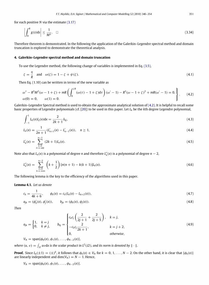
Fig. 1. Velocity profiles for s = 1 andm = 1 for several values ofM .

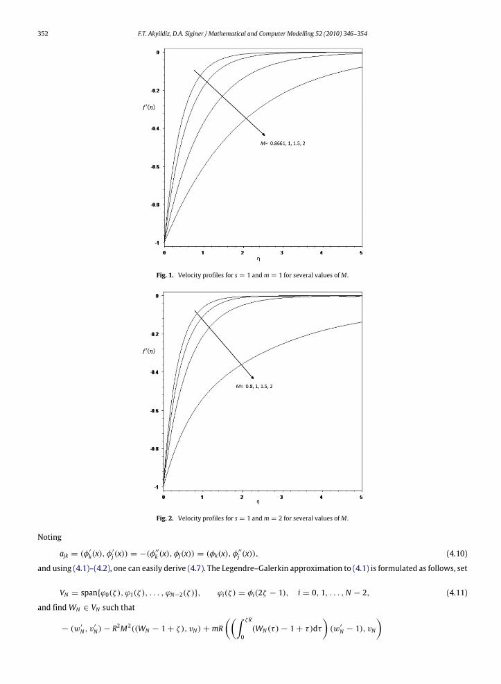
Fig. 2. Velocity profiles for s = 1 andm = 2 for several values ofM .

Noting

ajk = (φ′k(x), φ′

j (x)) = −(φ′′

k (x), φj(x)) = (φk(x), φ′′

j (x)), (4.10)

and using (4.1)–(4.2), one can easily derive (4.7). The Legendre–Galerkin approximation to (4.1) is formulated as follows, set

VN = spanϕ0(ζ ), ϕ1(ζ ), . . . , ϕN−2(ζ ), ϕi(ζ ) = φi(2ζ − 1), i = 0, 1, . . . ,N − 2, (4.11)

and findWN ∈ VN such that

− (w′N , v′

N)− R2M2((WN − 1+ ζ ), vN)+mR

((∫ ζR

0(WN(τ )− 1+ τ)dτ

)(w′N − 1), vN

)

F.T. Akyildiz, D.A. Siginer / Mathematical and Computer Modelling 52 (2010) 346–354 353

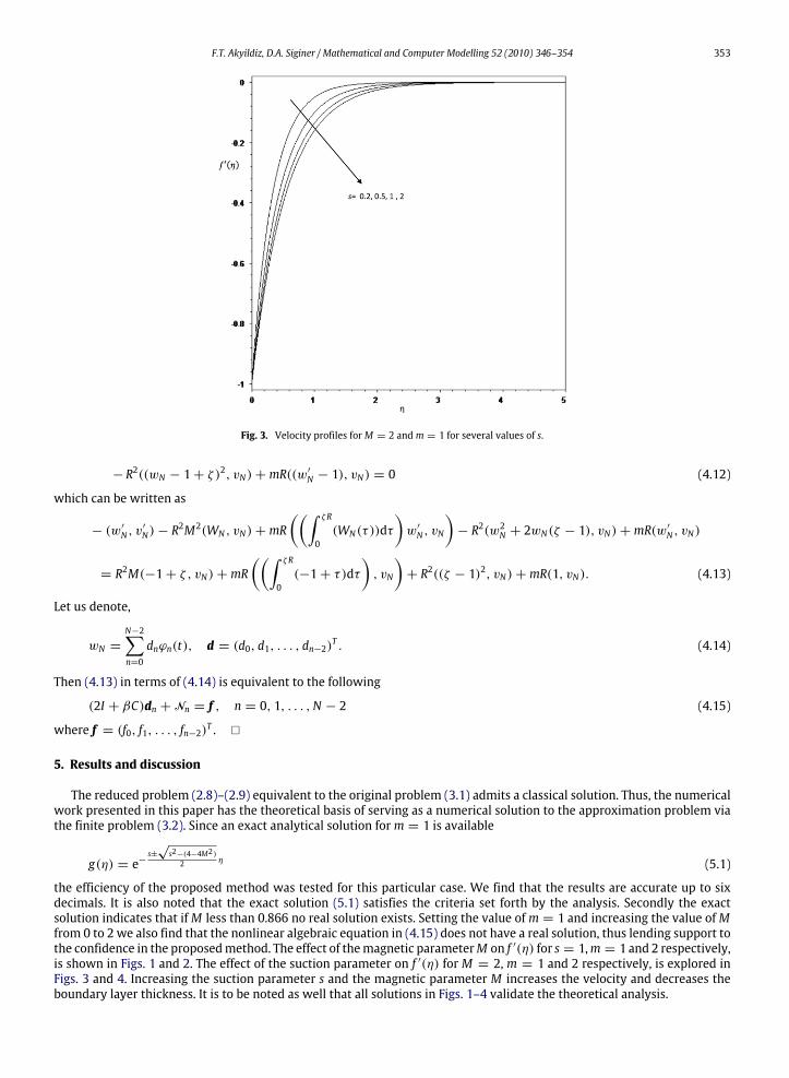
Fig. 3. Velocity profiles forM = 2 andm = 1 for several values of s.

− R2((wN − 1+ ζ )2, vN)+mR((w′N − 1), vN) = 0 (4.12)

which can be written as

− (w′N , v′

N)− R2M2(WN , vN)+mR

((∫ ζR

0(WN(τ ))dτ

)w′N , vN

)− R2(w2N + 2wN(ζ − 1), vN)+mR(w

′

N , vN)

= R2M(−1+ ζ , vN)+mR((∫ ζR

0(−1+ τ)dτ

), vN

)+ R2((ζ − 1)2, vN)+mR(1, vN). (4.13)

Let us denote,

wN =

N−2∑n=0

dnϕn(t), d = (d0, d1, . . . , dn−2)T . (4.14)

Then (4.13) in terms of (4.14) is equivalent to the following

(2I + βC)dn +Nn = f , n = 0, 1, . . . ,N − 2 (4.15)

where f = (f0, f1, . . . , fn−2)T .

5. Results and discussion

The reduced problem (2.8)–(2.9) equivalent to the original problem (3.1) admits a classical solution. Thus, the numericalwork presented in this paper has the theoretical basis of serving as a numerical solution to the approximation problem viathe finite problem (3.2). Since an exact analytical solution form = 1 is available

g(η) = e−s±√s2−(4−4M2)2 η (5.1)

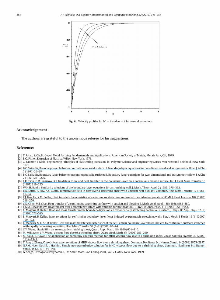
the efficiency of the proposed method was tested for this particular case. We find that the results are accurate up to sixdecimals. It is also noted that the exact solution (5.1) satisfies the criteria set forth by the analysis. Secondly the exactsolution indicates that ifM less than 0.866 no real solution exists. Setting the value ofm = 1 and increasing the value ofMfrom 0 to 2 we also find that the nonlinear algebraic equation in (4.15) does not have a real solution, thus lending support tothe confidence in the proposedmethod. The effect of themagnetic parameterM on f ′(η) for s = 1,m = 1 and 2 respectively,is shown in Figs. 1 and 2. The effect of the suction parameter on f ′(η) for M = 2, m = 1 and 2 respectively, is explored inFigs. 3 and 4. Increasing the suction parameter s and the magnetic parameter M increases the velocity and decreases theboundary layer thickness. It is to be noted as well that all solutions in Figs. 1–4 validate the theoretical analysis.

354 F.T. Akyildiz, D.A. Siginer / Mathematical and Computer Modelling 52 (2010) 346–354

Fig. 4. Velocity profiles forM = 2 andm = 2 for several values of s.

Acknowledgement

The authors are grateful to the anonymous referee for his suggestions.

References

[1] T. Altan, S. Oh, H. Gegel, Metal Forming Fundamentals and Applications, American Society of Metals, Metals Park, OH, 1979.[2] E.G. Fisher, Extrusion of Plastics, Wiley, New York, 1976.[3] Z. Tadmor, I. Klein, Engineering Principles of Plasticating Extrusion, in: Polymer Science and Engineering Series, Van Nostrand Reinhold, New York,1970.

[4] B.C. Sakiadis, Boundary-layer behavior on continuous solid surface: I. Boundary-layer equations for two-dimensional and axisymmetric flow, J. AIChe7 (1961) 26–28.

[5] B.C. Sakiadis, Boundary-layer behavior on continuous solid surface: II. Boundary-layer equations for two-dimensional and axisymmetric flow, J. AIChe7 (1961) 221–225.

[6] F.K. Tsou, E.M. Sparrow, R.J. Goldstain, Flow and heat transfer in the boundary-layer on a continuous moving surface, Int. J. Heat Mass Transfer 10(1967) 219–235.

[7] W.H.H. Banks, Similarity solutions of the boundary-layer equations for a stretching wall, J. Mech. Theor. Appl. 2 (1983) 375–392.[8] B.K. Dutta, P. Roy, A.S. Gupta, Temperature field in flow over a stretching sheet with uniform heat flux, Int. Commun. Heat Mass Transfer 12 (1985)89–94.

[9] L.J. Grubka, K.M. Bobba, Heat transfer characteristics of a continuous stretching surface with variable temperature, ASME J. Heat Transfer 107 (1985)248–250.

[10] C.K. Chen, M.I. Char, Heat transfer of a continuous stretching surface with suction and blowing, J. Math. Anal. Appl. 135 (1988) 568–580.[11] E.M.A. Elbashbeshy, Heat transfer over a stretching surface with variable surface heat flux, J. Phys. D: Appl. Phys. 31 (1998) 1951–1954.[12] E. Magyari, B. Keller, Heat and mass transfer in the boundary-layers on an exponentially stretching continuous surface, J. Phys. D: Appl. Phys. 32 (5)

(1999) 577–585.[13] E. Magyari, B. Keller, Exact solutions for self-similar boundary-layer flows induced by permeable stretching walls, Eur. J. Mech. B Fluids 19 (1) (2000)

109–122.[14] E. Magyari, M.E. Ali, B. Keller, Heat andmass transfer characteristics of the self-similar boundary-layer flows induced by continuous surfaces stretched

with rapidly decreasing velocities, Heat Mass Transfer 38 (1–2) (2001) 65–74.[15] C.Y. Wang, Liquid film on an unsteady stretching sheet, Quart. Appl. Math. 48 (1990) 601–610.[16] M. Miklavcic, C.Y. Wang, Viscous flow due to a shrinking sheet, Quart. Appl. Math. 64 (2006) 283–290.[17] M. Sajid, T. Hayat, The application of homotopy analysis method for MHD viscous flow due to a shrinking sheet, Chaos Solitons Fractals 39 (2009)

1317–1323.[18] T. Fang, J. Zhang, Closed-formexact solutions ofMHDviscous flowover a shrinking sheet, Commun.Nonlinear Sci. Numer. Simul. 14 (2009) 2853–2857.[19] N.F.M. Noor, Kechil, I. Hashim, Simple non-perturbative solution for MHD viscous flow due to a shrinking sheet, Commun. Nonlinear Sci. Numer.

Simul. 15 (2010) 144–148.[20] G. Szegö, Orthogonal Polynomials, in: Amer. Math. Soc. Colloq. Publ., vol. 23, AMS, New York, 1939.