EX ANTE ASSESSMENT OF POSSIBLE

EU-INDIA FTA: A GTAP ANALYSIS

Prof. Somesh Mathur

Rahul Arora

Ankit Jain

2014, November

INTRODUCTION

EU-India trade relations have advanced enormously over the last decade. The European Union and

India benefit from a longstanding relationship going back to the early 1960s. India and the EU

signed their first bilateral trade agreements in 1973. The most recent co-operation agreement was

signed in 1994 and an action plan was signed in 2005. As of April 2007, there have been

negotiations about a free trade agreement between the two which is anticipated to benefit both the

economies largely.

Current Statistics

Here are some statistics which defines the current situation of the EU and India worldwide.

1. GDP and Population: EU’s total share in world GDP accounts to almost 17.25% while

India accounts for nearly 6.64 % of the world’s GDP. Also the share in global population

of the EU and India is nearly 7.02% and 17.5% respectively.

2. FDI: During the financial year 2013-14 (i.e. during April 2013-March 2014), India has

received FDI equity inflows of US $ 24.30 billion which represents an 8% increase over

the FDI equity inflows of US$ 22.42 billion received during the corresponding period

(April 2012-March 2013) of the previous financial year (2012-13) but is very less

compared to big economies like USA, EU, China etc. The data on FDI inflows and outflows

is important for the discussion on FTA between the two as the nature of current deal heavily

depends on the restrictiveness of FDI.

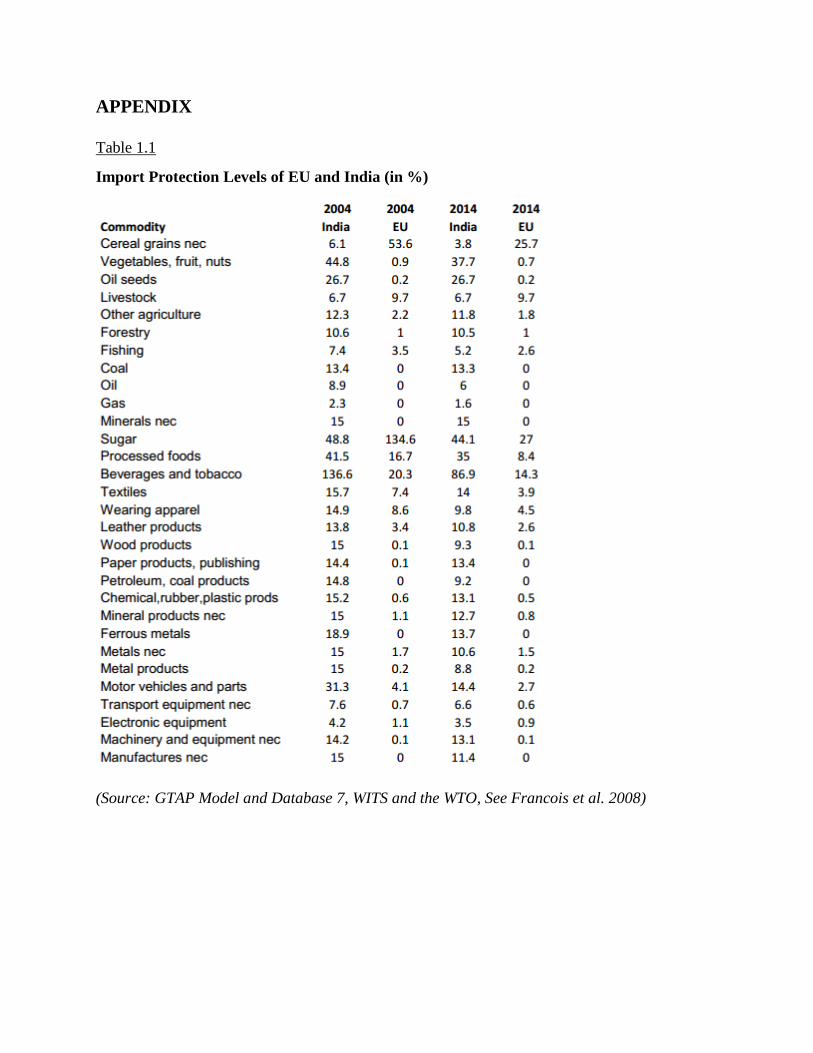
3. Import Protection: Due to agreements with various countries on tariff reduction for various

commodities, the levels of import protection in India has decreased. India has low levels

of import protection from EU than the US and on the other hand the EU has high levels of

import protection for Indian imports than the rest of the world imports. As can be seen from

Table 1.1 in the Appendix, the highest levels of import protection by India occurs in

Primary sector and in that for Beverages and Tobacco products, Sugar and Vegetables,

Fruits and Nuts and Processed Foods. For EU, the most protected sectors are again the

Processed Foods as in Sugar and in Agriculture it is Cereals, Grains etc.

Also for both India and EU, the Services sector is highly protected. Construction is the only

service in which both show low levels of protection. Also the total share of the highest

protected goods is less than 1.5 % of EU imports from India.

Trade Statistics

India is the eighth trading partner of EU accounting for nearly only 0.3% of European Foreign

Direct Investment, albeit provides India's largest source of investment. The EU is India’s largest

trading partner accounting for approximately € 72.7 billion in trade in goods and € 23.7 billion in

trade in services as of 2013.

TABLE 1: EU-India Trade 2011-2013, € billions

Year Trade in goods Trade in services

EU imports EU exports Balance

EU

imports EU exports Balance

2011 39.9 40.6 0.7 11 11.8 0.8

2012 37.4 38.5 1.1 10.7 11.8 1.1

2013 36.8 35.9 -0.9 11.2 12.5 1.3

Source: Eurostat Comext - Statistical regime 4

We can see that India’s major importing commodities from EU includes Pearls, Stones, and

Jewelry etc. (around 24%), Nuclear Reactors and Appliances (17.23%) and Electric Machinery

and Equipment, Medical Apparatus and Organic Chemicals (16.3%). And India’s major exporting

commodities include Mineral Fuels and Mineral Oils etc. (14.75%), Pearls, Stones, and Jewelry

etc. (6.75%) and Organic Chemicals (6.19%).

Based on all this information we can make the aggregation in different regions and commodities

to get the best results from GTAP Model.

GTAP Model

Although there are several general equilibrium models to evaluate the impact of the proposed

India-EU FTA but we use GTAP model for this purpose as it is the simplest and most organized

model. In this section is a brief overview of the GTAP model used in this assessment. The Global

Trade Analysis Project (GTAP) model was first formulated by Hertel in 1997. This is the most

widely used CGE model for the analysis of various trade policies. The GTAP model is multi-

region, multi-sector, computable general equilibrium model, with perfect competition and constant

returns to scale. The GTAP Model also gives a wide range of closure options, including

unemployment, tax revenue replacement and fixed trade balance closures, and a selection of partial

equilibrium closures. The model contains particular production and utility functions and assumes

that prices will adjust to clear all the markets. The factors included in the GTAP database are land,

skilled and unskilled labor, capital and natural resources. The benchmark year for this CGE

analysis is 2007.

Based on this current situation of the two economies, this study examines the possible effects of

the proposed EU-India FTA on several sectors and overall welfare, macroeconomic, and trade

variables using GTAP model and database.

LITERATURE REVIEW

Not much work (Ex Ante) has been done on the ongoing negotiations of EU-India FTA although

the negotiations first started in April 2007. But many researchers have worked on different FTAs

using different models to study the possible impact of any FTA between two or more economies.

Francois and Norberg (2008) used CGE framework projected through 2014 along with the

discussions of FDI patterns and restrictions. They conclude that the overall effect for India is

positive under all the scenarios and small but positive effects for EU countries too over the long

run. On the other hand there are negative effects on the rest of the world, and in that mainly the

developing ones. Achterbosch, Roza and Kuiper (2008) did a quantitative assessment of the EU-

India FTA. They also used the GTAP model and database, a global general equilibrium model

using 2004 as the base year. They predicted that the FTA would be in the interest of both the

partners. They also emphasize on the point that EU-India FTA delivers little scope for achieving

efficiency gains through adjustments to the pattern of International Specialization. They conclude

by saying that India can probably search other FTA partners as the only sector in which growth

purpose is fulfilled is the Agriculture sector. Decreux and Mitaritonna (2007) used the CEPII’s

CGE model (MIRAGE). For the initial protection level they have used the MAcMap database on

tariffs. They considered two scenarios, first, in which protection on services is cut by 10 % and

second in which it is cut by 25 %. They concluded that the overall impact on both the economies

would be positive, may it large or small.

On a separate remark, the studies of India’s FTA with other big economies like BRICS and

ASEAN also uses general equilibrium analysis. Sachin Kumar Sharma (2012) studied the BRICS

FTA using GTAP model and database with 2004 as the reference year. Nag and Sikdar (2011)

worked on the India-ASEAN FTA using the same computable general equilibrium model.

The present study seeks to fulfill the same for the EU-India FTA by using a general equilibrium

methodology which would help to assess the possible impact of the FTA on its members and other

countries.

DATA & METHODOLOGY

As discussed earlier in the introduction part, this assessment is carried out using the GTAP model

and database which is a multi-region model and assumes perfect competition, constant returns to

scale and profit and utility maximizing conduct. The overall structure and functioning of GTAP

model is explained in Hertel (1997). For this study we have done region and commodity wise

aggregation in the GTAP model. The GTAP database is benchmarked to the year 2007.

The Ex-Ante analysis/ Computable General Equilibrium (CGE) Analysis require detailed data on

the whole economy. This is because not only are inter-linkages present between various sectors of

an economy; sectors in an economy are also linked to the rest of the world. Thus, linkages are

present at the national, regional and global levels both in terms of products and in the input

markets. To get this data, this study will utilize GTAP 7 database. The database provides data on

57 different sectors and 134 different regions across the world. These 57 sectors have been linked

to 4 different sectors which consists of All Goods, Utility and Construction, Transport and

Communication and Other Services. Similar breakdown for 134 regions is done for the regional

aggregation and they are mapped to 10 different regions (India, EU27, North America, Latin

America, South Asia, West Asia, South East Asia, North Asia, East Asia and Rest of the World).

This type of aggregation is done due to the global importance of the mapped regions. The

aggregated regions would get influenced with the decisions made by India and the EU on this FTA

and it might cause changes in the future relations between India and the EU with these regions.

SECTORAL AGGREGATION

All Goods Utility and

Construction

Transportation

and

Communication

Other Services

Paddy, Rice Wheat Cereal Grain

Nec, Vegetable, Fruits, Oilseeds

Sugarcane, Sugar Beet

Plant Based Fiber, Crop Nec

Cattle,sheep, goat, horse

Animal Product Nec

Raw Milk, Wool,

Silk‐Worm Cocoons

Forestry, Fishing, Coal, Oil, Gas

Minerals nec

Meat: Cattle, Sheep, Goats, horse

Meat Products Nec

Vegetable Oils And Fats

Dairy Products

Processed Rice, Sugar

Food Product Nec

Beverages And Tobacco Products

Textiles, Wearing Apparel,

Leather Wood and paper products

Petroleum, plastic products

Minerals, Ferrous Metals and

products, Transport and Electric

Equipment, Machinery

Electricity,

Gas

Manufacture

And

Distribution,

Water,

Construction

Trade, Transport

nec,

Sea transport,

Air transport,

Communication

Financial Services nec,

Insurance,

Business Services nec,

Recreation and other

services,

PubAdmin/Defense

Health/Education,

Dwellings

REGIONAL AGGREGATION

India, East Asia (8 countries), North Asia and Russia (1 group), South East Asia (12 countries),

South Asia (7 countries), West Asia (15 countries), North America (4 countries), Latin America

(19 countries), EU 27, Rest of the world.

RESULTS

Major Macroeconomic Variables: GDP, Exports, Imports, Welfare’

This section of the study deals with the simulation results done in the GTAP model.

WELFARE EFFECTS

In the GTAP model, the net welfare gains are measured using the Equivalent Variation (EV) in

income. The welfare gain is decomposed into several components such as Allocative Efficiency

effect, terms of trade effect, and investment and savings effect. In the static GTAP model, which

has been used here, the population, endowment and technology remain fixed. So the only way to

increase welfare is to reduce the excess burden which arises from the existing distortions. Any

change in the allocative efficiency is directly propagated to the equilibrium conditions.

In case of Perfect Competition:

The GTAP model calculates the welfare change by analyzing a variable called EV

(Equivalent Variation). It computes a money metric equivalent of the utility change (which

is calculated using % change in aggregate per capita utility for a region) and any population

change in the region. It is measured in Million Dollars.

EV = E (U,Pi) – E (Ui,Pi), where E stands for expenditure, U for Utility, Pi for Initial price

level.

It is welfare improving to increase the level of a relatively taxed activity since this involves the

reallocation of a commodity or endowment from a low value use to a relatively high social

marginal usage. The same is true for endowments and for goods traded. Any good that yields trade

tax to the economy benefits the economy. Saving-investment term does not contribute to welfare

changes but both investment and savings appear in welfare decomposition. This is because

investment sales generate income but do not enter into regional utility while savings enter regional

utility but does not generate current income.

In GTAP modeling framework, regional household behavior is governed by an aggregate utility

function specified over per capita private household consumption, per capita government spending

and per capita savings. The percentage change in this aggregate per capita utility for a region is

the welfare change variable that is computed in a standard GTAP model during simulations. The

model computes a money metric equivalent of this utility change and any change in population in

the region. This convenient measure referred to as equivalent variation (EV) summarizes the

regional welfare changes resulting from any policy shock and is given in dollar values (US $

million). The regional household’s EV is given by the difference between the expenditure required

to obtain the post simulation level of utility at initial prices and that available initially.1

The welfare effect of the simulation are given below. (in million dollars)

Regions|WELFARE Allocative Efficiency Terms of Trade

Investment and Savings Total

India 603 -1181 -525 -1103

EastAsia -166 -597 360 -403

NorthAsia 46.9 -96.9 1.42 -48.7

SEAsia -68.2 -424 138 -354

SouthAsia 1.16 50.3 -38.7 12.7

WestAsia -159 -1336 303 -1193

NorthAmerica -30.9 -222 -414 -667

LatinAmerica -56 -181 31.5 -205

EU27 1339 5062 136 6538

RestofWorld -108 -1084 5.46 -1186

Total 1401 -8.6 -1.13 1392

It can be easily seen from the above simulation results that EU has gained the most in terms of

welfare effect and all other countries except South Asian Region experienced a welfare loss. The

welfare loss effect on India are unsuccessful due to the highly negative terms of trade effect and

negative investment and savings effect. The main reason behind this type of behavior is that in the

case of India, resources would divert from efficient sectors to inefficient sectors. As for the other

regions, West Asia also faces a welfare loss due to highly negative terms of trade effect.

GDP EFFECTS

The change in GDP is not only due to the trade liberalization but also due to all related effects due

to change in the trade policy of the country such as change in product demand, production pattern,

resource distribution, prices etc. Bigger economies would have more GDP growth, technically.

Below are the simulation results explaining macroeconomic effects for all the regions:

GDPEXP consumption investment Govt sp exports imports Total

India 727458 423873 133234 247223 -307638 1224150

EastAsia 4719527 2862039 1494675 2955936 -2480056 9552121

NorthAsia 668555 287701 237078 384356 -277997 1299694

SEAsia 712485 303319 125092 887921 -733910 1294907

SouthAsia 209842 63906 25801 47904 -81489 265964

WestAsia 656258 367092 263596 794646 -598806 1482785

NorthAmerica 11427074 3232948 2646317 2091897 -2888315 16509920

LatinAmerica 1728914 554580 479126 575268 -522215 2815672

EU27 9800967 3622681 3483340 5842554 -5927586 16821956

RestofWorld 2749156 1110775 708232 1517175 -1526868 4558470

Total 33400235 12828913 9596491 15344880 -15344880 55825639

As we can see from the above table that there is an increase in the GDP for all the present regions.

The EU27 and North American region will be most beneficial from this FTA in terms of GDP

gain. India will also benefit from the FTA but not to the extent of EU gain.

Terms of Trade: Terms of trade is defined as the relative price of exports in terms of imports and

is defined as the ratio of export prices to import prices. It can be interpreted as the amount of import

goods an economy can purchase per unit of export goods.

CHANGE IN EXPORTS AND IMPORTS

Table for change in imports

VIWS 1 India 2 East Asia

3 NorthAsia 4 SEAsia

5 SouthAsia

6 WestAsia

7 NorthAmerica

8 LatinAmerica 9 EU27

10 RestofWorld Total

1 AllGoods 16099 -2419 -170 -1830 -73 -3118 -1818 -869 19673 -2544 22931

2 Util_Cons 15 79 39 24 1 44 25 5 -257 70 43

3 TransComm 118 320 15 201 12 216 217 90 -1264 337 263

4 OthServices 157 347 29 231 17 327 744 121 -1836 443 582

Total 16389 -1672 -89 -1374 -42 -2530 -832 -654 16316 -1694 23819

Table for change in exports

VXWD 1 India

2 EastAsia

3 NorthAsia

4 SEAsia

5 SouthAsia

6 WestAsia

7 NorthAmerica

8 LatinAmerica

9 EU27

10 RestofWorld Total

1 AllGoods 15168 -2393 -158 -1644 -60 -3054 -1738 -461 19225 -2285 22597

2 Util_Cons 15 79 39 24 1 44 25 5 -257 70 43

3 TransComm 118 320 15 201 12 216 217 90 -1264 337 263

4 OthServices 157 347 29 231 17 327 744 121 -1836 443 582

Total 15457 -1647 -77 -1188 -30 -2465 -752 -247 15868 -1435 23484

As we can see from the above tables for imports and exports change, there is a major change in

imports as well as for EU27 in case of all goods sector and this is also true for India. While EU

faces negative change in exports and imports for all the other sectors in the economy and India has

a slight but positive increase in all the other sectors. For other countries, and rest of the world, all

changes in imports and exports of All Goods are negative.

CONCLUSIONS

This project used the General Equilibrium Analysis using the GTAP model and database on 134

regions linked to 10 different regions and 57 sectors mapped to 4 different sectors to analyze the

possible impact of the EU-India FTA. The reference year for the GTAP model is 2007. In this

study we reduced the tariffs for the All Goods sector to zero and saw what repercussions it has on

India and EU. We analyzed all the macroeconomic effects on both the economies and found that

in terms of welfare, India is on the losing side while EU gains a lot if the FTA is finalized. For the

GDP growth, every region is experiencing a positive gain in GDP through this FTA. It is revealed

that the change in imports and exports for EU in every sector except All Goods is negative while

it is positive for All goods sector for both India and EU. India faces small but positive effects on

the change in imports and exports for all the other sectors.

Basically if we see on the welfare side, India might get other beneficial FTA partners. As the

welfare loss in case of India is very high and not at all fruitful. Overall, the impact of the proposed

EU-India FTA would be negative for India and positive (highly) for EU. However at the

disaggregated level, results will vary across the 57 sectors.

REFERENCES

Joseph Francois, Hanna Norberg, Annette Pelkmans-Balaoing (2008), “Trade Impact Assessment

of an EU-India Free Trade Agreement”, Institute of International and Development Economics

(IIDE).

Trade Sustainability Impact Assessment for the FTA between the EU and the Republic of India

(2009), European Commission, DG-Trade.

Decreux, Yvan and Cristina Mitaronna (2007), Economic Impact of a Potential Free Trade

Agreement (FTA) between the European Union and India (Study commissioned by the

Directorate-General for Trade of the Commission of the European Union).

Arpita Mukherjee, Paul Wymenga (2013), “The Long Road towards an EU-India Free Trade

Agreement”, Directorate-General for External Policies of the Union.

Thom Achterbosch, Marijke Kuiper, Pim Roza (2008), “EU - India FTA - A Quantitative

Assessment”, LEI.

Jan Wouters, Idesbald Goddeeris, Bregt Natens and Filip Ciortuz (2013), “Some Critical Issues in

the EU-India Free Trade Agreement Negotiations”, Working Draft, KU Leuven.

Sachin Kumar Sharma, Murali Kallummal (2012), “A GTAP Analysis of the Proposed BRICS

Free Trade Agreement”, Working Draft, IIFT.

Biswajit Nag and Chandrima Sikdar (2011), “India-ASEAN FTA: Implication of Phased

Liberalization”, IIFT.

Michael G. Plummer, David Cheong, Shintaro Hamanaka (2010), “Methodology for Impact

Assessment of Free Trade Agreements”, Asian Development Bank.

WEBSITES : GTAP, WTO, Ministry of Commerce and Industry, WITS

APPENDIX

Table 1.1

Import Protection Levels of EU and India (in %)

(Source: GTAP Model and Database 7, WITS and the WTO, See Francois et al. 2008)