Identifying and Estimating the Distributions of Ex Post

and Ex Ante Returns to Schooling:

A Survey of Recent Developments∗

Flavio Cunha

University of Chicago

James J. Heckman

University of Chicago

February 18, 2006

∗This work was supported by NIH Grant R01-HD04311 and a grant from the Pew Foundation. Wewish to thank Lars Hansen, Lance Lochner, Salvador Navarro, Robert Townsend, Sergio Urzua, and PetraTodd for helpful comments.

Abstract

This paper surveys a recent body of research by Carneiro, Hansen, and Heckman (2001, 2003),Cunha and Heckman (2006), Cunha, Heckman, and Navarro (2005a,b, 2006), Heckman and Navarro(2006) and Navarro (2004) that estimates and identifies the ex post distribution of returns to school-ing and determines ex ante distributions of returns on which agents base their schooling choices.We discuss methods and evidence, and state a fundamental identification problem concerning theseparation of preferences, market structures and agent information sets. For a variety of marketstructures and preference specifications, we estimate that over 50% of the ex post variance in returnsto college are forecastable at the time agents make their schooling choices.

JEL Code: C31

Key Words: Ex Ante Returns to Schooling; Ex Post Returns to Schooling; Agent InformationSets.

Flavio Cunha James J. HeckmanDepartment of Economics Department of EconomicsUniversity of Chicago University of Chicago1126 E. 59th Street 1126 E. 59th StreetChicago, IL 60637 Chicago, IL 60637flavio@uchicago.edu jjh@uchicago.eduphone: 773-256-6216 phone: 773-702-0634fax: 773-702-8490 fax: 773-702-8490

1

1 Introduction

In computing ex ante returns to schooling, it is necessary to characterize what is in the agent’s

information set at the time schooling decisions are made. To do so, the recent literature exploits

the key idea that if agents know something and use that information in making their schooling

decisions, it will affect their schooling choices. With panel data on earnings we can measure realized

outcomes and assess what components of those outcomes were known at the time schooling choices

were made.1

The literature on panel data earnings dynamics (e.g. Lillard and Willis, 1978; MaCurdy, 1982)

is not designed to estimate what is in agent information sets. It estimates earnings equations of the

following type:

Yi,t = Xi,tβ + Siτ + U i,t, (1)

where Yi,t, Xi,t, Si, Ui,t denote (for person i at time t) the realized earnings, observable characteristics,

educational attainment, and unobservable characteristics, respectively, from the point of view of the

observing economist. The variables generating outcomes realized at time t may or may not have

been known to the agents at the time they made their schooling decisions.

The error term Ui,t is usually decomposed into two or more components. For example, it is

common to specify that

U i,t = φi + δi,t. (2)

The term φi is a person-specific effect. The error term δi,t is often assumed to follow an ARMA

(p, q) process (see Hause, 1980; MaCurdy, 1982) such as δi,t = ρδi,t−1 +mi,t, where mi,t is a mean

zero innovation independent of Xi,t and the other error components. The components Xi,t, φi, and

δi,t all contribute to measured ex post variability across persons. However, the literature is silent

about the difference between heterogeneity and uncertainty, the unforecastable part of earnings as

of a given age. The literature on income mobility and on inequality measures all variability ex post

as in Chiswick (1974), Mincer (1974) and Chiswick and Mincer (1972).

1An alternative approach summarized by Manski (2004) is to use survey methods to elicit expectations. We donot survey that literature in this paper.

2

An alternative specification of the error process postulates a factor structure for earnings,

U i,t = θiαt + εi,t, (3)

where θi is a vector of skills (e.g., ability, initial human capital, motivation, and the like), αt is a

vector of skill prices, and the εi,t are mutually independent mean zero shocks independent of θi.

Hause (1980) and Heckman and Scheinkman (1987) analyze such earnings models. Any process in

the form of equation (2) can be written in terms of (3). The latter specification is more directly

interpretable as a pricing equation than (2).

Depending on the available market arrangements for coping with risk, the predictable compo-

nents of Ui,t will have a different effect on choices and economic welfare than the unpredictable

components, if people are risk averse and cannot fully insure against uncertainty. Statistical de-

compositions based on (1), (2), and (3) or versions of them describe ex post variability but tell us

nothing about which components of (1) or (3) are forecastable by agents ex ante. Is φi unknown

to the agent? δi,t? Or φi + δi,t? Or mi,t? In representation (3), the entire vector θi, components of

the θi, the εi,t, or all of these may or may not be known to the agent at the time schooling choices

are made.

The methodology developed in Carneiro, Hansen, and Heckman (2003), Cunha, Heckman, and

Navarro (2005a,b) and Cunha and Heckman (2006) provides a framework within which it is possible

to identify components of life cycle outcomes that are forecastable and acted on at the time decisions

are taken from ones that are not. In order to choose between high school and college, agents forecast

future earnings (and other returns and costs) for each schooling level. Using information about

educational choices at the time the choice is made, together with the ex post realization of earnings

and costs that are observed at later ages, it is possible to estimate and test which components of

future earnings and costs are forecast by the agent. This can be done provided we know, or can

estimate, the earnings of agents under both schooling choices and provided we specify the market

environment under which they operate as well as their preferences over outcomes.

For certain market environments where separation theorems are valid, so that consumption de-

3

cisions are made independently of wealth maximizing decisions, it is not necessary to know agent

preferences to decompose realized earnings outcomes in this fashion. Carneiro, Hansen, and Heck-

man (2003), Cunha, Heckman, and Navarro (2005a,b) and Cunha and Heckman (2006) use choice

information to extract ex ante or forecast components of earnings and to distinguish them from

realized earnings under different market environments. The difference between forecast and realized

earnings allows them to identify the distributions of the components of uncertainty facing agents

at the time they make their schooling decisions.

2 A Generalized Roy Model

To state these issues more precisely, consider a version of the generalized Roy (1951) economy with

two sectors.2 Let Si denote different schooling levels. Si = 0 denotes choice of the high school

sector for person i, and Si = 1 denotes choice of the college sector. Each person chooses to be in

one or the other sector but cannot be in both. Let the two potential outcomes be represented by

the pair (Y0,i, Y1,i), only one of which is observed by the analyst for any agent. Denote by Ci the

direct cost of choosing sector 1, which is associated with choosing the college sector (e.g., tuition

and non-pecuniary costs of attending college expressed in monetary values).

Y1,i is the ex post present value of earnings in the college sector, discounted over horizon T for

a person choosing at a fixed age, assumed for convenience to be zero,

Y1,i =TXt=0

Y1,i,t

(1 + r)t,

and Y0,i is the ex post present value of earnings in the high school sector at age zero,

Y0,i =TXt=0

Y0,i,t

(1 + r)t,

where r is the one-period risk-free interest rate. Y1,i and Y0,i can be constructed from time se-

2See Heckman (1990) and Heckman and Smith (1998) for discussions of the generalized Roy model. In this paperwe assume only two schooling levels for expositional simplicity, although our methods apply more generally.

4

ries of ex post potential earnings streams in the two states: (Y0,i,0, . . . , Y0,i,T ) for high school and

(Y1,i,0, . . . , Y1,i,T ) for college. A practical problem is that we only observe one or the other of these

streams. This partial observability creates a fundamental identification problem which can be solved

using the methods described in Heckman, Lochner, and Todd (2006) and the references they cite.

The variables Y1,i, Y0,i, and Ci are ex post realizations of returns and costs, respectively. At the

time agents make their schooling choices, these may be only partially known to the agent, if at all.

Let Ii,0 denote the information set of agent i at the time the schooling choice is made, which is time

period t = 0 in our notation. Under a complete markets assumption with all risks diversifiable (so

that there is risk-neutral pricing) or under a perfect foresight model with unrestricted borrowing or

lending but full repayment, the decision rule governing sectoral choices at decision time ‘0’ is

Si =

⎧⎪⎨⎪⎩ 1, if E (Y1,i − Y0,i − Ci | Ii,0) ≥ 0

0, otherwise.3(4)

Under perfect foresight, the postulated information set would include Y1,i, Y0,i, and Ci. Under either

model of information, the decision rule is simple: one attends school if the expected gains from

schooling are greater than or equal to the expected costs. Thus under either set of assumptions,

a separation theorem governs choices. Agents maximize expected wealth independently of their

consumption decisions over time.

The decision rule is more complicated in the absence of full risk diversifiability and depends on

the curvature of utility functions, the availability of markets to spread risk, and possibilities for

storage. (See Cunha and Heckman, 2006, and Navarro, 2004, for a more extensive discussion.) In

these more realistic economic settings, the components of earnings and costs required to forecast

the gain to schooling depend on higher moments than the mean. In this paper we use a model

with a simple market setting to motivate the identification analysis of a more general environment

analyzed elsewhere (Carneiro, Hansen, and Heckman, 2003, and Cunha, Heckman, and Navarro,

2005a).

Suppose that we seek to determine Ii,0. This is a difficult task. Typically we can only partially3If there are aggregate sources of risk, full insurance would require a linear utility function.

5

identify Ii,0 and generate a list of candidate variables that belong in the information set. We

can usually only estimate the distributions of the unobservables in Ii,0 (from the standpoint of

the econometrician) and not individual person-specific information sets. Before describing their

analysis, we consider how this question might be addressed in the linear-in-the-parameters Card

(2001) model.

3 Identifying Information Sets in Card’s Model of School-

ing

We seek to decompose the “returns” coefficient or the gross gains from schooling in an earnings-

schooling model into components that are known at the time schooling choices are made and com-

ponents that are not known. For simplicity assume that, for person i, returns are the same at all

levels of schooling. Write discounted lifetime earnings of person i as

Yi = α+ ρiSi + U i, (5)

where ρi is the person-specific ex post return, Si is years of schooling, and Ui is a mean zero

unobservable. We seek to decompose ρi into two components ρi = ηi+ νi, where ηi is a component

known to the agent when he/she makes schooling decisions and νi is revealed after the choice

is made. Schooling choices are assumed to depend on what is known to the agent at the time

decisions are made, Si = λ (ηi, Zi, τ i), where the Zi are other observed determinants of schooling

and τ i represents additional factors unobserved by the analyst but known to the agent. Both of

these variables are in the agent’s information set at the time schooling choices are made. We seek

to determine what components of ex post lifetime earnings Yi enter the schooling choice equation.

If ηi is known to the agent and acted on, it enters the schooling choice equation. Otherwise it

does not. Component νi and any measurement errors in Y1,i or Y0,i should not be determinants

of schooling choices. Neither should future skill prices that are unknown at the time agents make

their decisions. If agents do not use ηi in making their schooling choices, even if they know it, ηi

6

would not enter the schooling choice equation. Determining the correlation between realized Yi and

schooling choices based on ex ante forecasts enables economists to identify components known to

agents and acted on in making their schooling decisions. Even if we cannot identify ρi, ηi, or νi for

each person, under conditions specified in this paper we can identify their distributions.

If we correctly specify the X and the Z that are known to the agent at the time schooling

choices are made, local instrumental variable estimates of the MTE identify ex ante gross gains.

Any dependence between the variables in the schooling equation and Y1−Y0 arises from information

known to the agent at the time schooling choices are made. If the conditioning set is misspecified by

using information on X and Z that accumulates after schooling choices are made and that predicts

realized earnings (but not ex ante earnings), the estimated return is an ex post return relative to

that information set. Thus, it is important to specify the conditioning set correctly to obtain the

appropriate ex ante return. The question is how to pick the information set? To exposit these ideas

we review the Card model.

3.1 The Card Model

A random coefficients model of the economic return to schooling has been an integral part of the

human capital literature since the papers by Becker and Chiswick (1966), Chiswick (1974), Chiswick

and Mincer (1972) and Mincer (1974). In its most stripped-down form and ignoring work experience

terms, the Mincer model writes log earnings for person i with schooling level Si as

ln yi = αi + ρiSi, (6)

where the “rate of return” ρi varies among persons as does the intercept, αi. For the purposes

of this discussion think of yi as an annualized flow of lifetime earnings. Unless the only costs of

schooling are earnings foregone, and markets are perfect, ρi is a percentage growth rate in earnings

with schooling and not a rate of return to schooling. Let αi = α+ εαi and ρi = ρ+ ερi where α and

ρ are the means of αi and ρi. Thus the means of εαi and ερi are zero. Earnings equation (6) can be

7

written as

ln yi = α+ ρSi + {εαi + ερiSi}. (7)

Equations (6) and (7) are the basis for a human capital analysis of wage inequality in which the

variance of log earnings is decomposed into components due to the variance in Si and components

due to the variation in the growth rate of earnings with schooling (the variance in ρ), the mean

growth rate across regions or time (ρ), and mean schooling levels (S). (See, e.g. Mincer, 1974, and

Willis, 1986.)

Given that the growth rate ρi is a random variable, it has become conventional to summarize the

distribution of growth rates by the mean, althoughmany other summarymeasures of the distribution

are possible. For the prototypical distribution of ρi, the conventional measure is the “average growth

rate” E(ρi) or E(ρi|X), where the latter conditions onX, the observed characteristics of individuals.

Other means are possible such as the mean growth rates for persons who attain a given level of

schooling.

The original Mincer model assumed that the growth rate of earnings with schooling, ρi, is

uncorrelated with or is independent of Si. This assumption is convenient but is not implied by

economic theory. It is plausible that the growth rate of earnings with schooling declines with the

level of schooling. It is also plausible that there are unmeasured ability or motivational factors that

affect the growth rate of earnings with schooling and are also correlated with the level of schooling.

Rosen (1977) discusses this problem in some detail within the context of hedonic models of schooling

and earnings. A similar problem arises in analyses of the impact of unionism on relative wages and

is discussed in Lewis (1963).

Allowing for correlated random coefficients (so Si is correlated with ερi) raises substantial prob-

lems that are just beginning to be addressed in a systematic fashion in the recent literature. Card’s

(2001) random coefficient model of the growth rate of earnings with schooling is derived from eco-

nomic theory and is based on the explicit analysis of Becker’s model by Rosen (1977).4 We consider

4Random coefficient models with coefficients correlated with the regressors are systematically analyzed in Heckmanand Robb (1985, 1986). See also Heckman and Vytlacil (1998). They originate in labor economics with the work ofLewis (1963). Heckman and Robb analyze training programs but their analysis applies to estimating the returns toschooling.

8

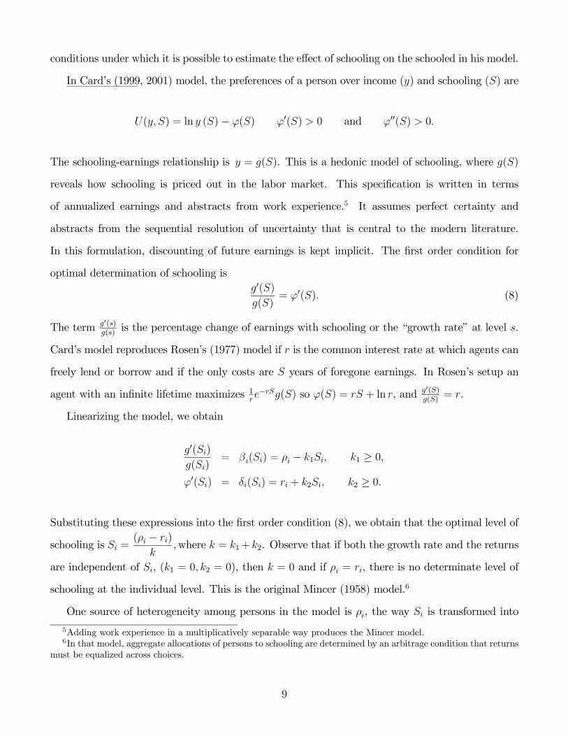
conditions under which it is possible to estimate the effect of schooling on the schooled in his model.

In Card’s (1999, 2001) model, the preferences of a person over income (y) and schooling (S) are

U(y, S) = ln y (S)− ϕ(S) ϕ0(S) > 0 and ϕ00(S) > 0.

The schooling-earnings relationship is y = g(S). This is a hedonic model of schooling, where g(S)

reveals how schooling is priced out in the labor market. This specification is written in terms

of annualized earnings and abstracts from work experience.5 It assumes perfect certainty and

abstracts from the sequential resolution of uncertainty that is central to the modern literature.

In this formulation, discounting of future earnings is kept implicit. The first order condition for

optimal determination of schooling isg0(S)

g(S)= ϕ0(S). (8)

The term g0(s)g(s)

is the percentage change of earnings with schooling or the “growth rate” at level s.

Card’s model reproduces Rosen’s (1977) model if r is the common interest rate at which agents can

freely lend or borrow and if the only costs are S years of foregone earnings. In Rosen’s setup an

agent with an infinite lifetime maximizes 1re−rSg(S) so ϕ(S) = rS + ln r, and g0(S)

g(S)= r.

Linearizing the model, we obtain

g0(Si)

g(Si)= βi(Si) = ρi − k1Si, k1 ≥ 0,

ϕ0(Si) = δi(Si) = ri + k2Si, k2 ≥ 0.

Substituting these expressions into the first order condition (8), we obtain that the optimal level of

schooling is Si =(ρi − ri)

k, where k = k1+k2. Observe that if both the growth rate and the returns

are independent of Si, (k1 = 0, k2 = 0), then k = 0 and if ρi = ri, there is no determinate level of

schooling at the individual level. This is the original Mincer (1958) model.6

One source of heterogeneity among persons in the model is ρi, the way Si is transformed into

5Adding work experience in a multiplicatively separable way produces the Mincer model.6In that model, aggregate allocations of persons to schooling are determined by an arbitrage condition that returns

must be equalized across choices.

9

earnings. (School quality may operate through the ρi for example, as in Behrman and Birdsall,

1983, and ρi may also differ due to inherent ability differences.) A second source of heterogeneity

is ri, the “opportunity cost” (cost of schooling) or “cost of funds.” Higher ability leads to higher

levels of schooling. Higher costs of schooling results in lower levels of schooling.

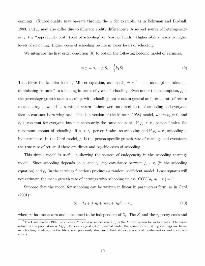
We integrate the first order condition (8) to obtain the following hedonic model of earnings,

ln yi = αi + ρiSi −1

2k1S

2i . (9)

To achieve the familiar looking Mincer equation, assume k1 = 0.7 This assumption rules out

diminishing “returns” to schooling in terms of years of schooling. Even under this assumption, ρi is

the percentage growth rate in earnings with schooling, but is not in general an internal rate of return

to schooling. It would be a rate of return if there were no direct costs of schooling and everyone

faces a constant borrowing rate. This is a version of the Mincer (1958) model, where k2 = 0, and

ri is constant for everyone but not necessarily the same constant. If ρi > ri, person i takes the

maximum amount of schooling. If ρi < ri, person i takes no schooling and if ρi = ri, schooling is

indeterminate. In the Card model, ρi is the person-specific growth rate of earnings and overstates

the true rate of return if there are direct and psychic costs of schooling.

This simple model is useful in showing the sources of endogeneity in the schooling earnings

model. Since schooling depends on ρi and ri, any covariance between ρi − ri (in the schooling

equation) and ρi (in the earnings function) produces a random coefficient model. Least squares will

not estimate the mean growth rate of earnings with schooling unless, COV (ρi, ρi − ri) = 0.

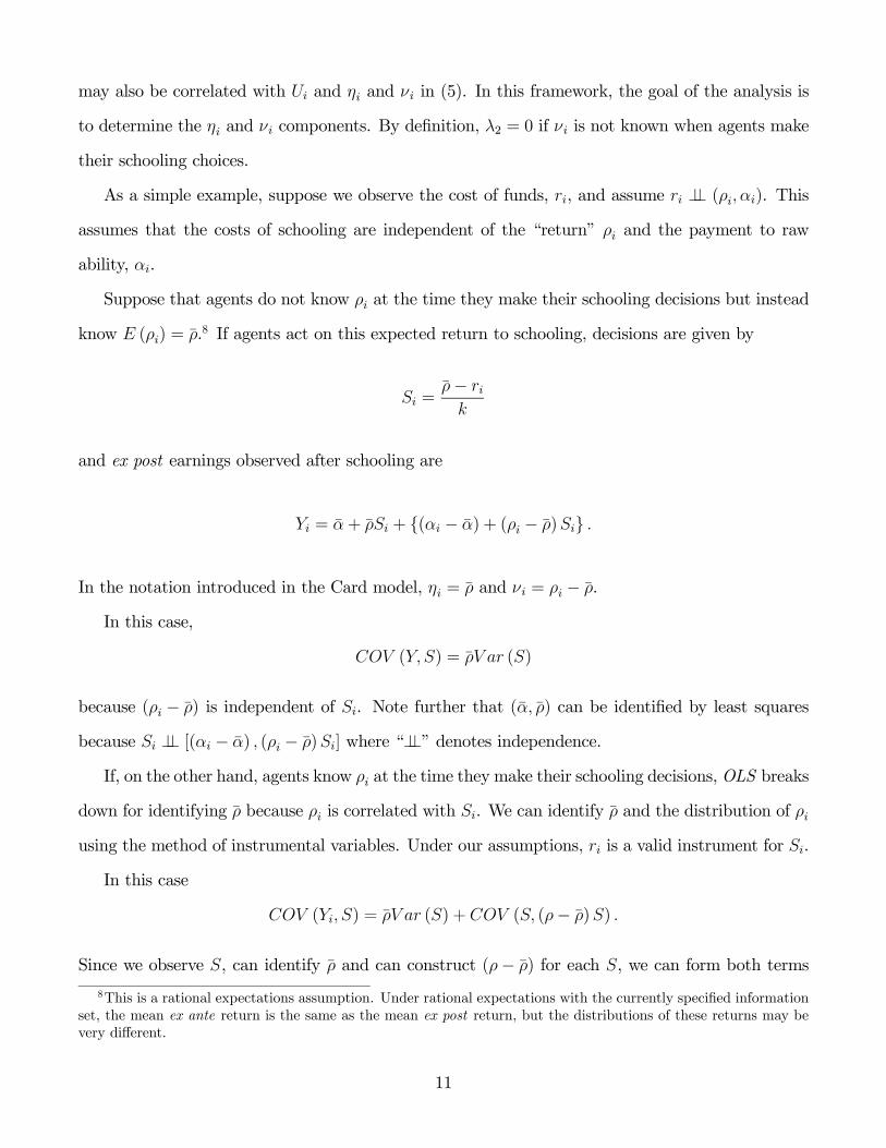
Suppose that the model for schooling can be written in linear in parameters form, as in Card

(2001):

Si = λ0 + λ1ηi + λ2νi + λ3Zi + τ i, (10)

where τ i has mean zero and is assumed to be independent of Zi. The Zi and the τ i proxy costs and

7The Card model (1999) produces a Mincer-like model where ρi is the Mincer return for individual i. The meanreturn in the population is E(ρi). It is an ex post return derived under the assumption that log earnings are linearin schooling, contrary to the literature, previously discussed, that shows pronounced nonlinearities and sheepskineffects.

10

may also be correlated with Ui and ηi and νi in (5). In this framework, the goal of the analysis is

to determine the ηi and νi components. By definition, λ2 = 0 if νi is not known when agents make

their schooling choices.

As a simple example, suppose we observe the cost of funds, ri, and assume ri ⊥⊥ (ρi, αi). This

assumes that the costs of schooling are independent of the “return” ρi and the payment to raw

ability, αi.

Suppose that agents do not know ρi at the time they make their schooling decisions but instead

know E (ρi) = ρ.8 If agents act on this expected return to schooling, decisions are given by

Si =ρ− rik

and ex post earnings observed after schooling are

Yi = α+ ρSi + {(αi − α) + (ρi − ρ)Si} .

In the notation introduced in the Card model, ηi = ρ and νi = ρi − ρ.

In this case,

COV (Y, S) = ρV ar (S)

because (ρi − ρ) is independent of Si. Note further that (α, ρ) can be identified by least squares

because Si ⊥⊥ [(αi − α) , (ρi − ρ)Si] where “⊥⊥” denotes independence.

If, on the other hand, agents know ρi at the time they make their schooling decisions, OLS breaks

down for identifying ρ because ρi is correlated with Si. We can identify ρ and the distribution of ρi

using the method of instrumental variables. Under our assumptions, ri is a valid instrument for Si.

In this case

COV (Yi, S) = ρV ar (S) + COV (S, (ρ− ρ)S) .

Since we observe S, can identify ρ and can construct (ρ− ρ) for each S, we can form both terms

8This is a rational expectations assumption. Under rational expectations with the currently specified informationset, the mean ex ante return is the same as the mean ex post return, but the distributions of these returns may bevery different.

11

on the right hand side. Under the assumption that agents do not know ρ but forecast it by ρ, ρ

is independent of S so we can test for independence directly. In this case the second term on the

right hand side is zero and does not contribute to the explanation of COV (ln y, S). Note further

that a Durbin (1954) — Wu (1973) — Hausman (1978) test can be used to compare the OLS and

IV estimates, which should be the same under the model that assumes that ρi is not known at the

time schooling decisions are made and that agents base their choice of schooling on E (ρi) = ρ. If

the economist does not observe ri, but instead observes determinants of ri that are exogenous, we

can still conduct the Durbin-Wu-Hausman test to discriminate between the two hypotheses, but we

cannot form COV (ρ, S) directly.

If we add selection bias to the Card model (so E (α | S) depends on S), we can identify ρ by IV

(Heckman and Vytlacil, 1998) but OLS is no longer consistent even if, in making their schooling

decisions, agents forecast ρi using ρ. Selection bias can occur, for example, if fellowship aid is given

on the basis of raw ability. In this case the Durbin-Wu-Hausman test is not helpful in assessing

what is in the agent’s information set.

Even ignoring selection bias, if we misspecify the information set, in the case where ri is not

observed, the proposed testing approach based on the Durbin-Wu-Hausman test breaks down. Thus

if we include the predictors of ri that predict ex post gains (ρi − ρ) and are correlated with Si, we

do not identify ρ. The Durbin-Wu-Hausman test is not informative on the stated question. For

example, if local labor market variables proxy the opportunity cost of school (the ri), and also

predict the evolution of ex post earnings (ρi − ρ), they are invalid. The question of determining the

appropriate information set is front and center and cannot in general be inferred using IV methods.

The method developed by Cunha, Heckman, and Navarro (2005a,b) and Cunha and Heckman

(2006) exploits the covariance between S and the realized Yt to determine which components of Yt

are known at the time schooling decisions are made. It explicitly models selection bias and allows

for measurement error in earnings. It does not rely on linearity of the schooling relationship in

terms of ρ− r. Their method recognizes the discrete nature of the schooling decision.

12

4 The Method of Cunha, Heckman and Navarro

Cunha, Heckman, and Navarro (2005a,b, henceforth CHN) and Cunha and Heckman (2006), exploit

covariances between schooling and realized earnings that arise under different information structures

to test which information structure characterizes the data. They build on the analysis of Carneiro,

Hansen, and Heckman (2003). To see how the method works, simplify the model to two schooling

levels. Heckman and Navarro (2006) extend this analysis to multiple schooling levels.

Suppose, contrary to what is possible, that the analyst observes Y0,i, Y1,i, and Ci. Such infor-

mation would come from an ideal data set in which we could observe two different lifetime earnings

streams for the same person in high school and in college as well as the costs they pay for attending

college. From such information, we could construct Y1,i − Y0,i −Ci. If we knew the information set

Ii,0 of the agent that governs schooling choices, we could also construct E (Y1,i − Y0,i − Ci | Ii,0).

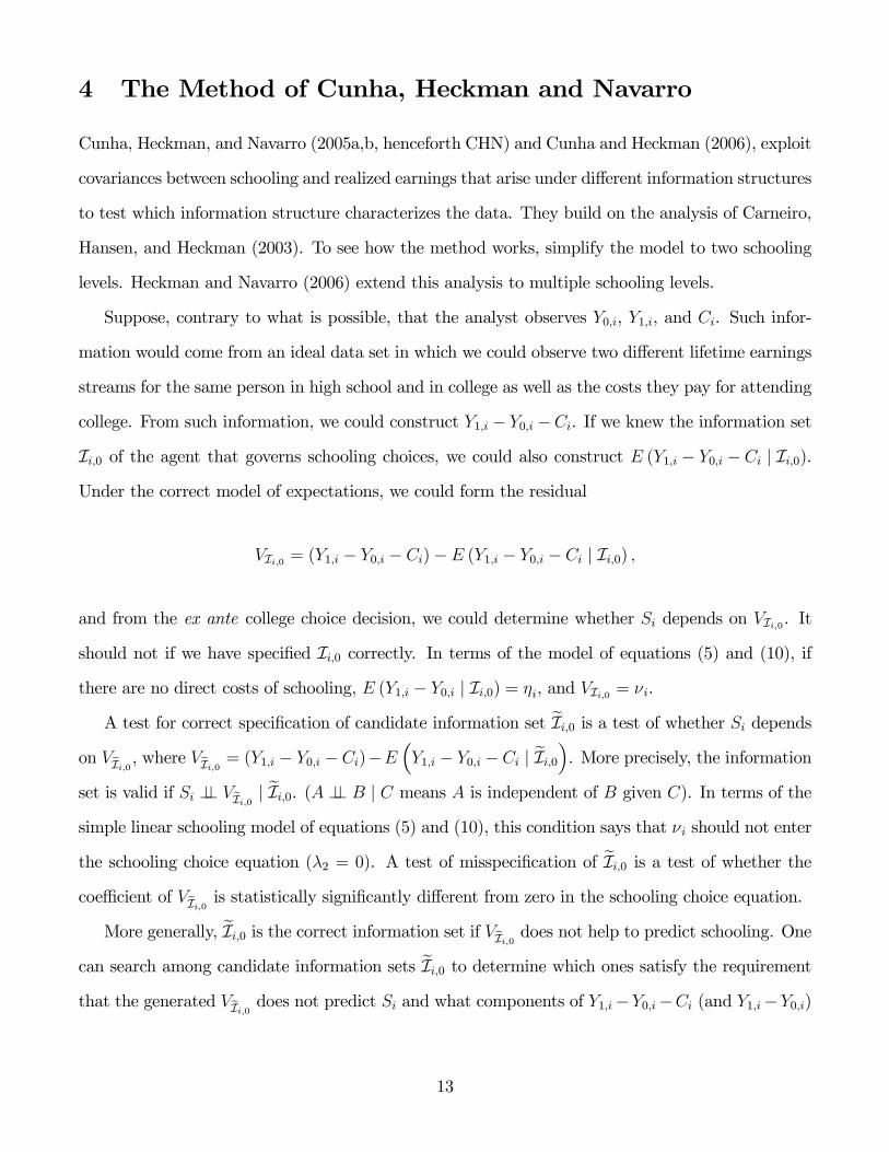
Under the correct model of expectations, we could form the residual

VIi,0 = (Y1,i − Y0,i − Ci)−E (Y1,i − Y0,i − Ci | Ii,0) ,

and from the ex ante college choice decision, we could determine whether Si depends on VIi,0. It

should not if we have specified Ii,0 correctly. In terms of the model of equations (5) and (10), if

there are no direct costs of schooling, E (Y1,i − Y0,i | Ii,0) = ηi, and VIi,0 = νi.

A test for correct specification of candidate information set eIi,0 is a test of whether Si dependson VIi,0 , where VIi,0 = (Y1,i − Y0,i − Ci)−E

³Y1,i − Y0,i − Ci | eIi,0´. More precisely, the information

set is valid if Si ⊥⊥ VIi,0 | eIi,0. (A ⊥⊥ B | C means A is independent of B given C). In terms of the

simple linear schooling model of equations (5) and (10), this condition says that νi should not enter

the schooling choice equation (λ2 = 0). A test of misspecification of eIi,0 is a test of whether thecoefficient of VIi,0 is statistically significantly different from zero in the schooling choice equation.

More generally, eIi,0 is the correct information set if VIi,0 does not help to predict schooling. Onecan search among candidate information sets eIi,0 to determine which ones satisfy the requirementthat the generated VIi,0 does not predict Si and what components of Y1,i−Y0,i−Ci (and Y1,i−Y0,i)

13

are predictable at the age schooling decisions are made for the specified information set.9 There may

be several information sets that satisfy this property.10 For a properly specified eIi,0, VIi,0 shouldnot cause (predict) schooling choices. The components of VIi,0 that are unpredictable are called

intrinsic components of uncertainty, as defined in this paper.

It is difficult to determine the exact content of Ii,0 known to each agent. If we could, we would

perfectly predict Si given our decision rule. More realistically, we might find variables that proxy

Ii,0 or their distribution. Thus, in the example of equations (5) and (10) we would seek to determine

the distribution of νi and the allocation of the variance of ρi to ηi and νi rather than trying to

estimate ρi, ηi, or νi for each person. This strategy is pursued in Cunha, Heckman, and Navarro

(2005b, 2006) for a two-choice model of schooling, and generalized by Cunha and Heckman (2006)

and Heckman and Navarro (2006).

4.1 An Approach Based on Factor Structures

Consider the following linear in parameters model for T periods. Write earnings in each counter-

factual state as

Y0,i,t = Xi,tβ0,t + U0,i,t,

Y1,i,t = Xi,tβ1,t + U1,i,t, t = 0, . . . , T.

We let costs of college be defined as

Ci = Ziγ + Ui,C .

Assume that the life cycle of the agent ends after period T . Linearity of outcomes in terms of

parameters is convenient but not essential to the method of CHN.

Suppose that there exists a vector of factors θi = (θi,1, θi,2, . . . , θi,L) such that θi,k and θi,j are

mutually independent random variables for k, j = 1, . . . , L, k 6= j. They represent the error term in

9This procedure is a Sims (1972) version of a Wiener-Granger causality test.10Thus different combinations of variables may contain the same information. The issue of the existence of a

smallest information set is a technical one concerning a minimum σ-algebra that satisfies the condition on Ii,0.

14

earnings at age t for agent i in the following manner:

U0,i,t = θiα0,t + ε0,i,t,

U1,i,t = θiα1,t + ε1,i,t,

where α0,t and α1,t are vectors and θi is a vector distributed independently across persons. The ε0,i,t

and ε1,i,t are mutually independent of each other and independent of the θi. We can also decompose

the cost function Ci in a similar fashion:

Ci = Ziγ + θiαC + εi,C .

All of the statistical dependence across potential outcomes and costs is generated by θ, X, and Z.

Thus, if we could match on θi (as well as X and Z), we could use matching to infer the distribution

of counterfactuals and capture all of the dependence across the counterfactual states through the

θi. However, in general, CHN allow for the possibility that not all of the required elements of θi are

observed.

The parameters αC and αs,t for s = 0, 1, and t = 0, . . . , T are the factor loadings. εi,C is

independent of the θi and the other ε components. In this notation, the choice equation can be

written as:

S∗i = E

ÃTXt=0

¡Xi,tβ1,t + θiα1,t + ε1,i,t

¢−¡Xi,tβ0,t + θiα0,t + ε0,i,t

¢(1 + r)t

− (Ziγ + θiαC + εiC)

¯¯ Ii,0

!Si = 1 if S∗ ≥ 0; Si = 0 otherwise. (11)

The term inside the parentheses is the discounted earnings of agent i in college minus the discounted

earnings of the agent in high school. The second term is the cost of college.

Constructing (11) entails making a counterfactual comparison. Even if the earnings of one

schooling level are observed over the lifetime using panel data, the earnings in the counterfactual

state are not. After the schooling choice is made, some components of the Xi,t, the θi, and the εi,t

may be revealed (e.g., unemployment rates, macro shocks) to both the observing economist and

15

the agent, although different components may be revealed to each and at different times. For this

reason, application of IV even in the linear schooling model is problematic. If the wrong information

set is used, the IV method will not identify the true ex ante returns.

Examining alternative information sets, one can determine which ones produce models for out-

comes that fit the data best in terms of producing a model that predicts date t = 0 schooling

choices and at the same time passes the CHN test for misspecification of predicted earnings and

costs. Some components of the error terms may be known or not known at the date schooling

choices are made. The unforecastable components are intrinsic uncertainty as CHN define it. The

forecastable information is called heterogeneity.11

To formally characterize the CHN empirical procedure, it is useful to introduce some additional

notation. Let¯ denote the Hadamard product (a¯b = (a1b1, . . . , aLbL)) for vectors a and b of length

L. This is a componentwise multiplication of vectors to produce a vector. Let ∆Xt, t = 0, . . . , T ,

∆Z, ∆θ, ∆εt, ∆εC , denote coefficient vectors associated with the Xt, t = 0, . . . , T , the Z, the θ, the

ε1,t− ε0,t, and the εC , respectively. These coefficients will be estimated to be nonzero in a schooling

choice equation if a proposed information set is not the actual information set used by agents. For

a proposed information set eIi,0 which may or may not be the true information set on which agentsact, CHN define the proposed choice index S∗i in the following way:

S∗i =TXt=0

E³Xi,t | eIi,0´(1 + r)t

¡β1,t − β0,t

¢+

TXt=0

hXi,t − E

³Xi,t | eIi,0´i

(1 + r)t¡β1,t − β0,t

¢¯∆Xt (12)

+E(θi | eIi,0)" TXt=0

(α1,t − α0,t)

(1 + r)t− αC

#+hθi − E

³θi | eIi,0´i(" TX

t=0

(α1,t − α0,t)

(1 + r)t− αC

#¯∆θ

)

+TXt=0

E³ε1,i,t − ε0,i,t | eIi,0´(1 + r)t

+TXt=0

h(ε1,i,t − ε0,i,t)−E

³ε1,i,t − ε0,i,t | eIi,0´i

(1 + r)t∆εt

−E³Zi | eIi,0´ γ − hZi −E

³Zi | eIi,0´i γ ¯∆Z − E

³εiC | eIi,0´− hεiC −E

³εiC | eIi,0´i∆εC .

To conduct their test, CHN fit a schooling choice model based on the proposed model (12). They

11The term ‘heterogeneity’ is somewhat unfortunate. Under this term, CHN include trends common across all peo-ple (e.g., macrotrends). The real distinction they are making is between components of realized earnings forecastableby agents at the time they make their schooling choices vs. components that are not forecastable.

16

estimate the parameters of the model including the ∆ parameters. This decomposition for S∗i

assumes that agents know the β, the γ, and the α.12 If it is not correct, the presence of additional

unforecastable components due to unknown coefficients affects the interpretation of the estimates.

A test of no misspecification of information set eIi,0 is a joint test of the hypothesis that the ∆ are

all zero. That is, when eIi,0 = Ii,0 then the proposed choice index eS∗i = S∗i .

In a correctly specified model, the components associated with zero ∆j are the unforecastable

elements or the elements which, even if known to the agent, are not acted on in making schooling

choices. To illustrate the application of the method of CHN, assume for simplicity that the Xi,t, the

Zi, the εi,C , the β1,t, β0,t, the α1,t, α0,t, and αC are known to the agent, and the εj,i,t are unknown

and are set at their mean zero values. We can infer which components of the θi are known and acted

on in making schooling decisions if we postulate that some components of θi are known perfectly

at date t = 0 while others are not known at all, and their forecast values have mean zero given Ii,0.

If there is an element of the vector θi, say θi,2 (factor 2), that has nonzero loadings (coefficients)

in the schooling choice equation and a nonzero loading on one or more potential future earnings, then

one can say that at the time the schooling choice is made, the agent knows the unobservable captured

by factor 2 that affects future earnings. If θi,2 does not enter the choice equation but explains future

earnings, then θi,2 is unknown (not predictable by the agent) at the age schooling decisions are made.

An alternative interpretation is that the second component ofhPT

t=0(α1,t−α0,t)(1+r)t

− αC

iis zero, i.e.,

that even if the component is known, it is not acted on. CHN can only test for what the agent

knows and acts on.

One plausible scenario case is that for their model εi,C is known (since schooling costs are

incurred up front), but the future ε1,i,t and ε0,i,t are not, have mean zero, and are insurable. If there

are components of the εj,i,t that are predictable at age t = 0, they will induce additional dependence

between Si and future earnings that will pick up additional factors beyond those initially specified.

The CHN procedure can be generalized to consider all components of (12). With it, the analyst

can test the predictive power of each subset of the overall possible information set at the date the

12CHN and Cunha and Heckman (2006) relax this assumption.

17

schooling decision is being made.13 ,14

In the context of the factor structure representation for earnings and costs, the contrast between

the CHN approach to identifying components of intrinsic uncertainty and the approach followed in

the literature is as follows. The traditional approach, as exemplified by Keane and Wolpin (1997),

assumes that the θi are known to the agent while the {ε0,i,t, ε1,i,t}Tt=0 are not.15 The CHN approach

allows the analyst to determine which components of θi and {ε0,i,t, ε1,i,t}Tt=0 are known and acted

on at the time schooling decisions are made.

Statistical decompositions do not tell us which components of (3) are known at the time agents

make their schooling decisions. A model of expectations and schooling is needed. If some of the

components of {ε0,i,t, ε1,i,t}Tt=0 are known to the agent at the date schooling decisions are made and

enter (12), then additional dependence between Si and future Y1,i − Y0,i due to the {ε0,i,t, ε1,i,t}Tt=0,

beyond that due to θi, would be estimated.

It is helpful to contrast the dependence between Si and future Y0,i,t, Y1,i,t arising from θi and

the dependence between Si and the {ε0,i,t, ε1,i,t}Tt=0. Some of the θi in the ex post earnings equation

may not appear in the choice equation. Under other information sets, some additional dependence

between Si and {ε0,i,t, ε1,i,t}Tt=0 may arise. The contrast between the sources generating realized

earnings outcomes and the sources generating dependence between Si and realized earnings is the

essential idea in the analysis of CHN. The method can be generalized to deal with nonlinear prefer-

13This test has been extended to a nonlinear setting, allowing for credit constraints, preferences for risk, and thelike. See Cunha, Heckman, and Navarro (2005a) and Navarro (2004).14A similar but distinct idea motivates the Flavin (1981) test of the permanent income hypothesis and her measure-

ment of unforecastable income innovations. She picks a particular information set eIi,0 (permanent income constructedfrom an assumed ARMA (p, q) time series process for income, where she estimates the coefficients given a specifiedorder of the AR and MA components) and tests if VIi,0 (our notation) predicts consumption. Her test of ‘excesssensitivity’ can be interpreted as a test of the correct specification of the ARMA process that she assumes generateseIi,0 which is unobserved (by the economist), although she does not state it that way. Blundell and Preston (1998)and Blundell, Pistaferri, and Preston (2004) extend her analysis but, like her, maintain an a priori specification ofthe stochastic process generating Ii,0. Blundell, Pistaferri, and Preston (2004) claim to test for ‘partial insurance.’In fact their procedure can be viewed as a test of their specification of the stochastic process generating the agent’sinformation set. More closely related to the analysis of CHN is the analysis of Pistaferri (2001), who uses the dis-tinction between expected starting wages (to measure expected returns) and realized wages (to measure innovations)in a consumption analysis.15Keane and Wolpin assume one factor where the θ is a discrete variable and they assume all factor loadings are

identical across periods. However, their specification of the uniquenesses or innovations is more general than thatused in factor analysis. The analysis of Hartog and Vijverberg (2002) is another example and uses variances of expost income to proxy ex ante variability, removing “fixed effects” (person specific θ).

18

ences and imperfect market environments.16 A central issue, discussed next, is how far one can go

in identifying income information processes without specifying preferences, insurance, and market

environments.

5 More general preferences and market settings

To focus on the main ideas in the literature, we have used the simple market structures of complete

contingent claims markets. What can be identified in more general environments? In the absence

of perfect certainty or perfect risk sharing, preferences and market environments also determine

schooling choices. The separation theorem allowing consumption and schooling decisions to be

analyzed in isolation that has been used thus far breaks down.

If we postulate information processes a priori, and assume that preferences are known up to

some unknown parameters as in Flavin (1981), Blundell and Preston (1998) and Blundell, Pista-

ferri, and Preston (2004), we can identify departures from specified market structures. Cunha,

Heckman, and Navarro (2005a) postulate an Aiyagari (1994) — Laitner (1992) economy with one

asset and parametric preferences to identify the information processes in the agent’s information

set. They take a parametric position on preferences and a nonparametric position on the economic

environment and the information set.

An open question, not yet fully resolved in the literature, is how far one can go in nonparamet-

16In a model with complete autarky with preferences Ψ, ignoring costs,

Ii =TXt=0

E

"Ψ¡Xi,tβ1,t + θiα1,t + ε1,i,t

¢−Ψ

¡Xi,tβ0,t + θiα0,t + ε0,i,t

¢(1 + ρ)t

¯¯ eIi,0

#,

where ρ is the time rate of discount, we can make a similar decomposition but it is more complicated given thenonlinearity in Ψ. For this model we could do a Sims noncausality test where

VIi,0 =TXt=0

Ψ¡Xi,tβ1,t + θiα1,t + ε1,i,t

¢−Ψ

¡Xi,tβ0,t + θiα0,t + ε0,i,t

¢(1 + ρ)

t

−TXt=0

E

"Ψ¡Xi,tβ1,t + θiα1,t + ε1,i,t

¢−Ψ

¡Xi,tβ0,t + θiα0,t + ε0,i,t

¢(1 + ρ)t

¯¯ eIi,0

#.

This requires some specification of Ψ. See Carneiro, Hansen, and Heckman (2003), who assume Ψ(Y ) = lnY and thatthe equation for lnY is linear in parameters. Cunha, Heckman, and Navarro (2005a) and Navarro (2004) generalizethat framework to a model with imperfect capital markets where some lending and borrowing is possible.

19

rically jointly identifying preferences, market structures and information sets. Cunha, Heckman,

and Navarro (2005a) add consumption data to the schooling choice and earnings data to secure

identification of risk preference parameters (within a parametric family) and information sets, and

to test among alternative models for market environments. Alternative assumptions about what

analysts know produce different interpretations of the same evidence. The lack of full insurance

interpretation given to the empirical results by Flavin (1981) and Blundell, Pistaferri, and Preston

(2004) may be a consequence of their misspecification of the agent’s information set generating

process. We now present some evidence on ex ante vs. ex post returns based on the analysis of

Cunha and Heckman (2006).

6 Evidence on Uncertainty and Heterogeneity of Returns

Few data sets contain the full life cycle of earnings along with the test scores and schooling choices

needed to directly estimate the CHN model and extract components of uncertainty. It is necessary

to pool data sets. See CHN who combine NLSY and PSID data sets. We summarize the analysis of

Cunha and Heckman (2006) in this subsection. See their paper for their exclusions and identification

conditions.

Following the preceding theoretical analysis, they consider only two schooling choices: high

school and college graduation.17 For simplicity and familiarity, we focus on their results based on

complete contingent claims markets. Because they assume that all shocks are idiosyncratic and the

operation of complete markets, schooling choices are made on the basis of expected present value

income maximization. Carneiro, Hansen, and Heckman (2003) assume the absence of any credit

markets or insurance. Cunha, Heckman, and Navarro (2005a) check whether their empirical findings

about components of income inequality are robust to different assumptions about the availability

of credit markets and insurance markets. They estimate an Aiyagari-Laitner economy with a single

asset and borrowing constraints and discuss risk aversion and the relative importance of uncertainty.

We summarize the evidence from alternative assumptions about market structures below.

17Heckman and Navarro (2006) present a model with multiple schooling levels.

20

6.1 Identifying Joint Distributions of Counterfactuals and the Role of

Costs and Ability as Determinants of Schooling

Suppose that the error term for Ys,t is generated by a two factor model,

Ys,t = Xβs,t + θ1αs,t,1 + θ2αs,t,2 + εs,t. (13)

We omit the “i” subscripts to eliminate notational burden. Cunha and Heckman (2006) report that

two factors are all that is required to fit the data.

They use a test score system of K ability tests:

TjT = XTωjT + θ1αjT + εjT , j = 1, . . . ,K (14)

Thus factor 1 is identified as an ability component. The cost function C is specified by:

C = Zγ + θ1αC,1 + θ2αC,2 + εC . (15)

They assume that agents know the coefficients of the model and X, Z, εC and some, but not

necessarily all, components of θ. Let the components known to the agent be θ. The decision rule

for attending college is based on:

S∗ = E

ÃTXt=0

Y1,t − Y0,t

(1 + r)t| X, θ

!− E

¡C | Z,X, θ, εC

¢(16)

S = 1 (S∗ ≥ 0) .

Cunha and Heckman (2006) report evidence that the estimated factors are highly nonnormal.18

18They assume that each factor k ∈ {1, 2} is generated by a mixture of Jk normal distributions,

θk ∼JkXj=1

pk,jφ¡fk | µk,j , τk,j

¢,

where the pk,j are the weights on the normal components.

21

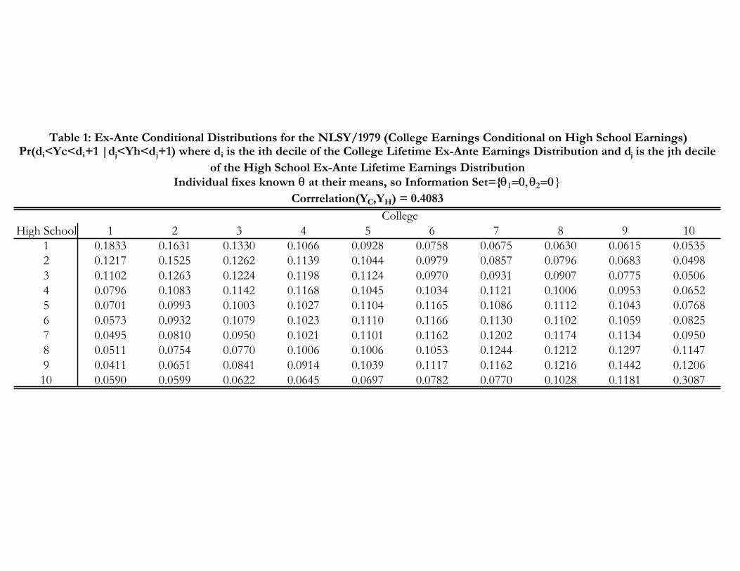
Table 1 presents the conditional distribution of ex post potential college earnings given ex post

potential high school earnings, decile by decile, as reported by Cunha and Heckman (2006). The

table displays a positive dependence between the relative positions of individuals in the two distri-

butions. However, the dependence is far from perfect. For example, about 10% of those who are at

the first decile of the high school distribution would be in the fourth decile of the college distribu-

tion. Note that this comparison is not being made in terms of positions in the overall distribution

of earnings. CHN can determine where individuals are located in the distribution of population

potential high school earnings and the distribution of potential college earnings although in the data

we only observe them in either one or the other state. Their evidence shows that the assumption of

perfect dependence across components of counterfactual distributions that is maintained in much

of the recent literature (e.g. Juhn, Murphy, and Pierce, 1993) is far too strong.

Figure 1 presents the marginal densities of predicted (actual) earnings for high school students

and counterfactual college earnings for actual high school students. When we compare the densities

of present value of earnings in the college sector for persons who choose college against the coun-

terfactual densities of college earnings for high school graduates we can see that many high school

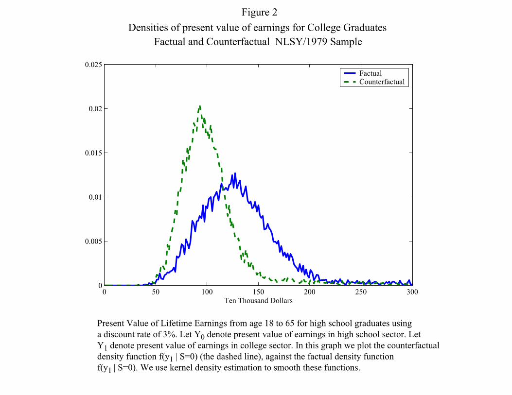
graduates would earn more as college graduates. In Figure 2 we repeat the exercise, this time for

college graduates.

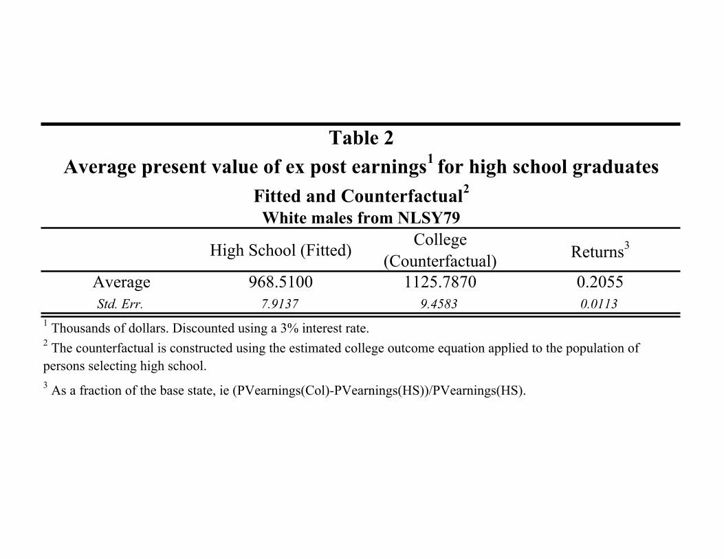
Table 2 from Cunha and Heckman (2006) reports the fitted and counterfactual present value of

earnings for agents who choose high school. The typical high school student would earn $968.51

thousand dollars over the life cycle. She would earn $1,125.78 thousand if she had chosen to be a

college graduate.19 This implies a return of 20% to a college education over the whole life cycle

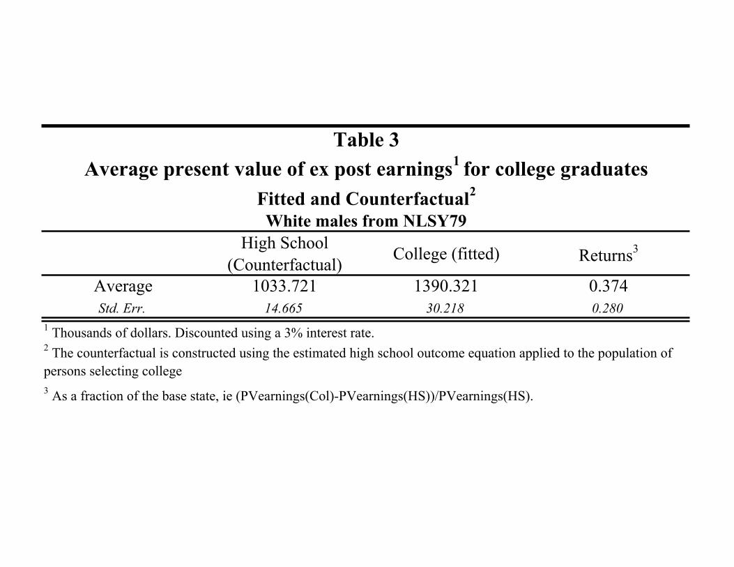
(i.e., a monetary gain of $157.28 thousand dollars). In table 3, from Cunha and Heckman (2006),

the typical college graduate earns $1,390.32 thousand dollars (above the counterfactual earnings of

what a typical high school student would earn in college), and would make only $1,033.72 thousand

dollars over her lifetime if she chose to be a high school graduate instead. The returns to college

education for the typical college graduate (which in the literature on program evaluation is referred

to as the effect of Treatment on the Treated) is around 38% above that of the return for a high

19These numbers may appear to be large but are a consequence of using a 3% discount rate.

22

school graduate.

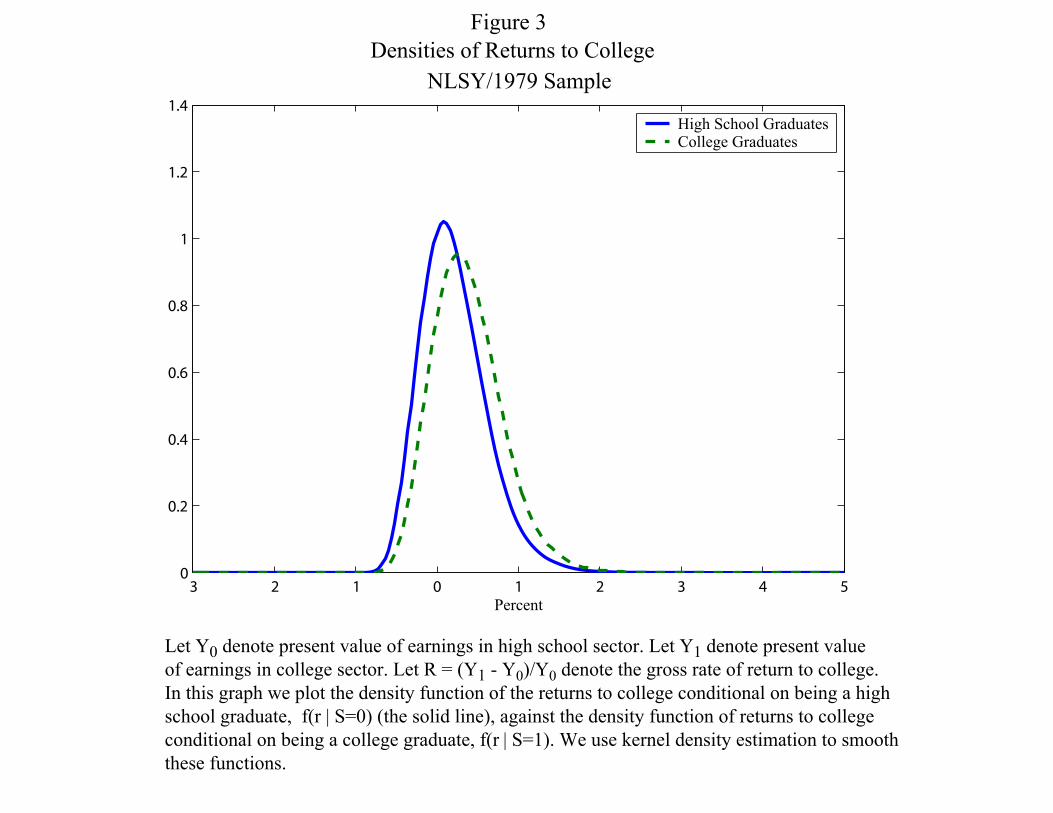
Figure 3 plots the density of ex post gross returns to education excluding direct costs and

psychic costs for agents who are high school graduates (the solid curve), and the density of returns

to education for agents who are college graduates (the dashed curve). In reporting our estimated

returns, CHN follow conventions in the literature on the returns to schooling and present growth

rates in terms of present values, and not true rates of return. Thus they insure option values.

These figures thus report the growth rates in present values³PV (1)−PV (0)

PV (0)

´where “1” and “0” refer

to college and high school and all present values are discounted to a common benchmark level.

Tuition and psychic costs are ignored. College graduates have returns distributed somewhat to the

right of high school graduates, so the difference is not only a difference for the mean individual but

is actually present over the entire distribution. An economic interpretation of figure 3 is that agents

who choose a college education are the ones who tend to gain more from it.

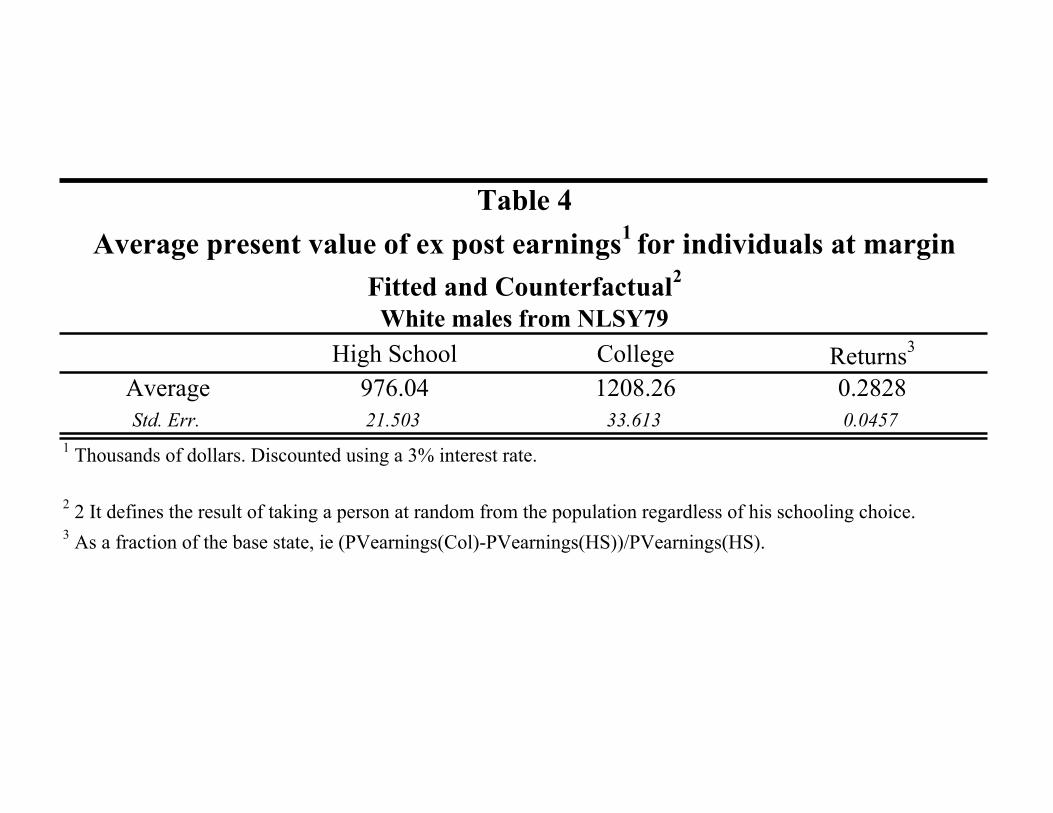
With their methodology, CHN can also determine returns to the marginal student. Table 4

reveals that the average individual who is just indifferent between a college education and a high

school diploma earns $976.04 thousand dollars as a high school graduate or $1,208.26 thousand

dollars as a college graduate. This implies a return of 28%. The returns to people at the margin are

above those of the typical high school graduate, but below those for the typical college graduate.

Since persons at the margin are more likely to be affected by a policy that encourages college

attendance, their returns are the ones that should be used in order to compute the marginal benefit

of policies that induce people into schooling.

6.2 Ex ante and Ex post Returns: Heterogeneity versus Uncertainty

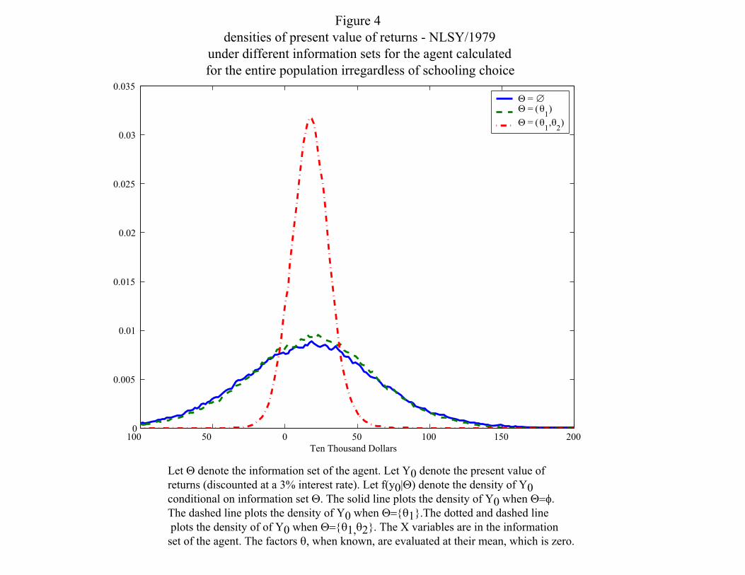
Figures 4 through 6, from Cunha and Heckman (2006) separate the effect of heterogeneity from

uncertainty in earnings. The figures plot the distribution of ex ante and ex post outcomes. The

information set of the agent is I = {X,Z,XT , εC ,Θ}, Θ contains some or all of the factors. In

their papers, the various information sets consist of different components of θ. We first consider

figure 4. It presents results for a variety of information sets. First assume that agents do not

know their factors; consequently, Θ = ∅. This is the case in which all of the unobservables are

23

treated as unknown by the agent, and, as a result, the density has a large variance. If we assume

that the agents know factor 1 but not factor 2,20 so that Θ = {θ1}, there is a reduction in the

forecast variance, but it is small. Factor 1, which is associated with cognitive ability, is important

for forecasting educational choices, but does not do a very good job in forecasting earnings. The

third case is the one in which the agent knows both factors, which is the case we test and cannot

reject. The agent is able to substantially reduce the forecast variance of earnings in high school.

Note the the variance in this case is much smaller than in the other two cases. Figure 6 reveals

much the same story about the college earnings distribution.

Table 5 presents the variance of potential earnings in each state, and returns under different

information sets available to the agent. We conduct this exercise for lifetime earnings, and report

baseline variances and covariances without conditioning and state the remaining uncertainty as a

fraction of the baseline no-information state variance when different components of θ are known to

the agents. CHN–who estimate a three factor model–show that both θ1 and θ2 are known to the

agents at the time they make their schooling decisions, but not θ3.

This discussion sheds light on the issue of distinguishing predictable heterogeneity from uncer-

tainty. CHN demonstrate that there is a large dispersion in the distribution of the present value of

earnings. This dispersion is largely due to heterogeneity, which is forecastable by the agents at the

time they are making their schooling choices. CHN provide tests that determine that agents know

θ1 and θ2. The remaining dispersion is due to luck, or uncertainty or unforecastable factors as of

age 17. Its contribution is smaller.

It is interesting to note that knowledge of the factors enables agents to make better forecasts.

Figure 6 presents an exercise for returns to college (Y1 − Y0) similar to that presented in figures 4

and 5 regarding information sets available to the agent. Knowledge of factor 2 also greatly improves

the forecastability of returns. 56% of the variability in returns is forecastable at age 18. The levels

also show high predictability (65% for high school; 56% for college). Most variability across people

is due to heterogeneity and not uncertainty. However there is still a lot of variability in agent

earnings after accounting for what is in the agent’s information set. This is intrinsic uncertainty at

20As opposed to the econometrician who never gets to observe either θ1 or θ2.

24

the time agents make their schooling choices.

6.3 Ex Ante versus Ex Post

Once the distinction between heterogeneity and uncertainty is made, it is possible to be precise about

the distinction between ex ante and ex post decision making. From their analysis, CHN conclude

that, at the time agents pick their schooling, the ε’s in their earnings equations are unknown to

them. These are the components that correspond to “luck.” It is clear that decision making would

be different, at least for some individuals, if the agent knew these chance components when choosing

schooling levels, since the decision rule would be based on (4) where all components of Y1,i, Y0,i,

and Ci are known, and no expectation need be taken.

If individuals could pick their schooling level using their ex post information (i.e., after learn-

ing their luck components in earnings) 13.81% of high school graduates would rather be college

graduates and 17.15% of college graduates would have stopped their schooling at the high school

level. Using the estimated counterfactual distributions, it is possible to consider a variety of policy

counterfactuals on distributions of outcomes locating persons in pre- and post-policy distributions.

They analyze for example, how tuition subsidies move people from one quantile of a Y0 distribution

to another quantile of a Y1 distribution. See Carneiro, Hansen, and Heckman (2001, 2003), Cunha,

Heckman, and Navarro (2005b, 2006) and Cunha and Heckman (2006) for examples of this work.

7 Extensions and Alternative Specifications

Carneiro, Hansen, and Heckman (2003) estimate a version of the model just presented for an en-

vironment of complete autarky. Individuals have to live within their means each period. Cunha,

Heckman, and Navarro (2005a) estimate a version of this model with restriction on intertemporal

trade as in the Aiyagari-Laitner economy. Different assumptions about credit markets and prefer-

ences produce a range of estimates of the proportion of the total variability of returns to schooling

that are unforecastable, ranging from 37% (Carneiro, Hansen, and Heckman, 2003) for a model

with complete autarky and log preferences, to 53% (CHN) for complete markets, to 44% (Cunha

25

and Heckman, 2006) for another complete market economy.

This line of work has just begun. It shows what is possible with rich panel data. The empirical

evidence on the importance of uncertainty is not yet settled. Yet most of the papers developed within

this research program suggest a substantial role for uncertainty in producing returns. Accounting

for uncertainty and psychic costs may help to explain the sluggish response of schooling enrollment

rates to rising returns to schooling that is documented in Ellwood and Kane (2000) and Card and

Lemieux (2001) because of the wedge between utility and money returns.

8 Models with Sequential Updating of Information

We have thus far discussed one shot models of schooling choice. In truth, schooling is a sequential

decision process made with increasingly richer information sets at later stages of the choice process.

Keane and Wolpin (1997) and Eckstein and Wolpin (1999) pioneered the estimation of dynamic

discrete choice models for analyzing schooling choices. They assume a complete market environment

and do not consider the range of possible alternative market structures facing agents. In the notation

of this paper, they assume a one (discrete) factor model with factor loadings that are different

across different counterfactual states, but are constant over time (αs,t = αs, s = 1, . . . , S where

there are S states).21 At a point in time, t, εs,t, s = 1, . . . , S are assumed to be multivariate normal

random variables. Over time the εt = (ε1,t, . . . , εs,t) are assumed to be independent and identically

distributed. They assume agents know θ but not the εt, t = 0, . . . , T . The unobservables are thus

equicorrelated over time (age) because the factor loadings are assumed equal over time and εt is

independent and identically distributed over time. They make parametric normality assumptions

in estimating their models. They impose and do not test the particular information structure that

they use.22 In their model, about 90% of the variance in lifetime returns is predictable at age 16.

Their estimate is at the extreme boundary of the estimates produced from the CHN analysis.

21Thus instead of assuming that θ is continuous, as do CHN, they impose that θ is a discrete-valued randomvariable that assumes a finite, known number of values.22Keane and Wolpin (1997) impose their discrete factor in the schooling choice and outcome equations rather than

testing for whether or not the factor appears in both sets of equations in the fashion of CHN as previously described.

26

Heckman and Navarro (2006) formulate and identify semiparametric sequential schooling models

based on the factor structures exposited in this paper. Like Keane and Wolpin, they assume that a

complete contingent claims market governs the data. They report substantial effects on empirical

estimates from relaxing normality assumptions. Using their framework, it is possible to test among

alternative information structures about the arrival of information on the components of vector θ at

different stages of the life cycle. Preliminary analysis based on their model supports the analysis of

CHN in finding a sizable role for heterogeneity (predictable variability) in accounting for measured

variability. They estimate the sequential reduction of uncertainty as information is acquired. Their

analysis shows that estimated option values for attending college are relatively small (at most 2%

of the total return). This is consistent with a lot of information known about future returns at

the time schooling decisions are being made. If their results hold up in subsequent analyses and

replications, they imply that the theoretical possibilities that arise from accounting for option values

may be empirically unimportant in computing rates of return.23

9 Summary and Conclusions

This paper surveys the main models and methods developed in Carneiro, Hansen, and Heckman

(2003), Cunha, Heckman, and Navarro (2005a,b, 2006), Cunha and Heckman (2006) and Heck-

man and Navarro (2006) for estimating models of heterogeneity and uncertainty in the returns to

schooling. The goal of this work is to separate variability from uncertainty and to estimate the

distributions of ex ante and ex post returns to schooling. The key idea in the recent literature is

to exploit the relationship between realized earnings and schooling choice equations to determine

which components of realized earnings are in agent information sets at the time they make their

schooling decisions. For a variety of market environments and assumptions about preferences, a

robust empirical regularity is that over 50% of the ex post variance in the returns to schooling are

forecastable at the time students make their college choices.

23Assuming that initial conditions are known by agents, the estimates of Keane and Wolpin (1997) are consistentwith small option values although they do not report the option values implicit in their estimates.

27

References

Aiyagari, S. R. (1994, August). Uninsured Idiosyncratic Risk and Aggregate Saving. Quarterly

Journal of Economics 109 (3), 659—684.

Becker, G. S. and B. R. Chiswick (1966, March). Education and the Distribution of Earnings. The

American Economic Review 56 (1/2), 358—369.

Behrman, J. R. and N. Birdsall (1983, December). The Quality of Schooling: Quantity Alone is

Misleading. American Economic Review 73 (5), 928—946.

Blundell, R., L. Pistaferri, and I. Preston (2004, October). Consumption inequality and partial

insurance. Technical Report WP04/28, Institute for Fiscal Studies.

Blundell, R. and I. Preston (1998, May). Consumption Inequality and Income Uncertainty. Quar-

terly Journal of Economics 113 (2), 603—640.

Card, D. (1999). The Causal Effect of Education on Earnings. In O. Ashenfelter and D. Card

(Eds.), Handbook of Labor Economics, Volume 5, pp. 1801—1863. New York: North-Holland.

Card, D. (2001, September). Estimating the Return to Schooling: Progress on Some Persistent

Econometric Problems. Econometrica 69 (5), 1127—1160.

Card, D. and T. Lemieux (2001, May). Can Falling Supply Explain the Rising Return to College

for Younger Men? A Cohort-Based Analysis. Quarterly Journal of Economics 116(2), 705—746.

Carneiro, P., K. Hansen, and J. J. Heckman (2001, Fall). Removing the Veil of Ignorance in

Assessing the Distributional Impacts of Social Policies. Swedish Economic Policy Review 8 (2),

273—301.

Carneiro, P., K. Hansen, and J. J. Heckman (2003, May). Estimating Distributions of Treatment

Effects with an Application to the Returns to Schooling and Measurement of the Effects of

Uncertainty on College Choice. International Economic Review 44 (2), 361—422. 2001 Lawrence

R. Klein Lecture.

28

Chiswick, B. R. (1974). Income Inequality: Regional Analyses Within a Human Capital Framework.

New York: National Bureau of Economic Research.

Chiswick, B. R. and J. Mincer (1972, May/June). Time-Series Changes in Personal Income Inequal-

ity in the United States from 1939, with Projections to 1985. Journal of Political Economy 80 (3

(Part II)), S34—S66.

Cunha, F. and J. J. Heckman (2006). A Framework for the Analysis of Inequality. Journal of

Macroeconomics, forthcoming.

Cunha, F., J. J. Heckman, and S. Navarro (2005a, August). The Evolution of Earnings Risk in the

US Economy. Presented at the 9th World Congress of the Econometric Society, London. Previ-

ously “Separating Heterogeneity from Uncertainty in an Aiyagari-Laitner Economy,” presented

at the Goldwater Conference on Labor Markets, Arizona State University, March 2004.

Cunha, F., J. J. Heckman, and S. Navarro (2005b, April). Separating Uncertainty from Heterogene-

ity in Life Cycle Earnings, The 2004 Hicks Lecture. Oxford Economic Papers 57 (2), 191—261.

Cunha, F., J. J. Heckman, and S. Navarro (2006). Counterfactual Analysis of Inequality and Social

Mobility. In S. L. Morgan, D. B. Grusky, and G. S. Fields (Eds.), Mobility and Inequality:

Frontiers of Research from Sociology and Economics, Chapter 4. Palo Alto: Stanford University

Press. Forthcoming.

Durbin, J. (1954). Errors in Variables. Review of the International Statistical Institute 22, 23—32.

Eckstein, Z. and K. I. Wolpin (1999, November). Why Youths Drop Out of High School: The

Impact of Preferences, Opportunities, and Abilities. Econometrica 67 (6), 1295—1339.

Ellwood, D. T. and T. J. Kane (2000). Who Is Getting a College Education? Family Background

and the Growing Gaps in Enrollment. In S. Danziger and J. Waldfogel (Eds.), Securing the Future:

Investing in Children from Birth to College, pp. 283—324. New York: Russell Sage Foundation.

Flavin, M. A. (1981, October). The Adjustment of Consumption to Changing Expectations About

Future Income. Journal of Political Economy 89 (5), 974—1009.

29

Hartog, J. and W. Vijverberg (2002, February). Do Wages Really Compensate for Risk Aversion

and Skewness Affection? Technical Report IZA DP No. 426, IZA, Bonn, Germany.

Hause, J. C. (1980, May). The Fine Structure of Earnings and the On-the-Job Training Hypothesis.

Econometrica 48 (4), 1013—1029.

Hausman, J. A. (1978, November). Specification Tests in Econometrics. Econometrica 46, 1251—

1272.

Heckman, J. J. (1990, May). Varieties of Selection Bias. American Economic Review 80 (2), 313—

318.

Heckman, J. J., L. J. Lochner, and P. E. Todd (2006). Earnings Equations and Rates of Return:

The Mincer Equation and Beyond. In E. A. Hanushek and F. Welch (Eds.), Handbook of the

Economics of Education. Amsterdam: North-Holland. forthcoming.

Heckman, J. J. and S. Navarro (2006). Dynamic Discrete Choice and Dynamic Treatment Effects.

Journal of Econometrics, forthcoming.

Heckman, J. J. and R. Robb (1985). Alternative Methods for Evaluating the Impact of Interventions.

In J. Heckman and B. Singer (Eds.), Longitudinal Analysis of Labor Market Data, Volume 10,

pp. 156—245. New York: Cambridge University Press.

Heckman, J. J. and R. Robb (1986). Alternative Methods for Solving the Problem of Selection Bias

in Evaluating the Impact of Treatments on Outcomes. In H. Wainer (Ed.), Drawing Inferences

from Self-Selected Samples, pp. 63—107. New York: Springer-Verlag. Reprinted in 2000, Mahwah,

NJ: Lawrence Erlbaum Associates.

Heckman, J. J. and J. Scheinkman (1987, April). The Importance of Bundling in a Gorman-

Lancaster Model of Earnings. Review of Economic Studies 54 (2), 243—355.

Heckman, J. J. and J. A. Smith (1998). Evaluating the Welfare State. In S. Strom (Ed.), Economet-

rics and Economic Theory in the Twentieth Century: The Ragnar Frisch Centennial Symposium,

pp. 241—318. New York: Cambridge University Press.

30

Heckman, J. J. and E. J. Vytlacil (1998, Fall). Instrumental Variables Methods for the Correlated

Random Coefficient Model: Estimating the Average Rate of Return to Schooling When the

Return Is Correlated with Schooling. Journal of Human Resources 33 (4), 974—987.

Juhn, C., K. M. Murphy, and B. Pierce (1993, June). Wage Inequality and the Rise in Returns to

Skill. Journal of Political Economy 101 (3), 410—442.

Keane, M. P. and K. I. Wolpin (1997, June). The Career Decisions of Young Men. Journal of

Political Economy 105 (3), 473—522.

Laitner, J. (1992, December). Random Earnings Differences, Lifetime Liquidity Constraints, and

Altruistic Intergenerational Transfers. Journal of Economic Theory 58 (2), 135—170.

Lewis, H. G. (1963). Unionism and Relative Wages in the United States: An Empirical Inquiry.

Chicago: University of Chicago Press.

Lillard, L. A. and R. J. Willis (1978, September). Dynamic Aspects of Earning Mobility. Econo-

metrica 46(5), 985—1012.

MaCurdy, T. E. (1982, January). The Use of Time Series Processes to Model the Error Structure

of Earnings in a Longitudinal Data Analysis. Journal of Econometrics 18 (1), 83—114.

Manski, C. F. (2004, September). Measuring Expectations. Econometrica 72 (5), 1329—1376.

Mincer, J. (1958, August). Investment in Human Capital and Personal Income Distribution. Journal

of Political Economy 66 (4), 281—302.

Mincer, J. (1974). Schooling, Experience and Earnings. New York: Columbia University Press for

National Bureau of Economic Research.

Navarro, S. (2004). Understanding Schooling: Using Observed Choices to Infer Agent’s Information

in a Dynamic Model of Schooling Choice when Consumption Allocation is Subject to Borrowing

Constraints. Unpublished manuscript, University of Chicago, Department of Economics.

31

Pistaferri, L. (2001, August). Superior Information, Income Shocks, and the Permanent Income

Hypothesis. Review of Economics and Statistics 83 (3), 465—476.

Rosen, S. (1977). Human Capital: A Survey of Empirical Research. In R. Ehrenberg (Ed.), Research

in Labor Economics, Volume 1, pp. 3—40. Greenwich, CT: JAI Press.

Roy, A. (1951, June). Some Thoughts on the Distribution of Earnings. Oxford Economic Pa-

pers 3(2), 135—146.

Sims, C. A. (1972, September). Money, Income, and Causality. American Economic Review 62 (4),

540—552.

Willis, R. J. (1986). Wage Determinants: A Survey and Reinterpretation of Human Capital Earnings

Functions. In O. Ashenfelter and R. Layard (Eds.), Handbook of Labor Economics, Volume, pp.

525—602. New York: North-Holland.

Wu, D. (1973, July). Alternative Tests of Independence between Stochastic Regressors and Distur-

bances. Econometrica 41, 733—750.

32

High School 1 2 3 4 5 6 7 8 9 101 0.1833 0.1631 0.1330 0.1066 0.0928 0.0758 0.0675 0.0630 0.0615 0.05352 0.1217 0.1525 0.1262 0.1139 0.1044 0.0979 0.0857 0.0796 0.0683 0.04983 0.1102 0.1263 0.1224 0.1198 0.1124 0.0970 0.0931 0.0907 0.0775 0.05064 0.0796 0.1083 0.1142 0.1168 0.1045 0.1034 0.1121 0.1006 0.0953 0.06525 0.0701 0.0993 0.1003 0.1027 0.1104 0.1165 0.1086 0.1112 0.1043 0.07686 0.0573 0.0932 0.1079 0.1023 0.1110 0.1166 0.1130 0.1102 0.1059 0.08257 0.0495 0.0810 0.0950 0.1021 0.1101 0.1162 0.1202 0.1174 0.1134 0.09508 0.0511 0.0754 0.0770 0.1006 0.1006 0.1053 0.1244 0.1212 0.1297 0.11479 0.0411 0.0651 0.0841 0.0914 0.1039 0.1117 0.1162 0.1216 0.1442 0.120610 0.0590 0.0599 0.0622 0.0645 0.0697 0.0782 0.0770 0.1028 0.1181 0.3087

College

Table 1: Ex-Ante Conditional Distributions for the NLSY/1979 (College Earnings Conditional on High School Earnings)Pr(di<Yc<di+1 |dj<Yh<dj+1) where di is the ith decile of the College Lifetime Ex-Ante Earnings Distribution and dj is the jth decile

of the High School Ex-Ante Lifetime Earnings DistributionIndividual fixes known at their means, so Information Set={

Corrrelation(YC,YH) = 0.4083

High School (Fitted) College(Counterfactual) Returns3

Average 968.5100 1125.7870 0.2055Std. Err. 7.9137 9.4583 0.0113

Table 2

3 As a fraction of the base state, ie (PVearnings(Col)-PVearnings(HS))/PVearnings(HS).

1 Thousands of dollars. Discounted using a 3% interest rate.2 The counterfactual is constructed using the estimated college outcome equation applied to the population of persons selecting high school.

Average present value of ex post earnings1 for high school graduatesFitted and Counterfactual2

White males from NLSY79

High School (Counterfactual) College (fitted) Returns3

Average 1033.721 1390.321 0.374Std. Err. 14.665 30.218 0.280

Table 3

3 As a fraction of the base state, ie (PVearnings(Col)-PVearnings(HS))/PVearnings(HS).

1 Thousands of dollars. Discounted using a 3% interest rate.2 The counterfactual is constructed using the estimated high school outcome equation applied to the population of persons selecting college

Average present value of ex post earnings1 for college graduatesFitted and Counterfactual2

White males from NLSY79

High School College Returns3

Average 976.04 1208.26 0.2828Std. Err. 21.503 33.613 0.0457

1 Thousands of dollars. Discounted using a 3% interest rate.

2 2 It defines the result of taking a person at random from the population regardless of his schooling choice.3 As a fraction of the base state, ie (PVearnings(Col)-PVearnings(HS))/PVearnings(HS).

Table 4Average present value of ex post earnings1 for individuals at margin

Fitted and Counterfactual2

White males from NLSY79

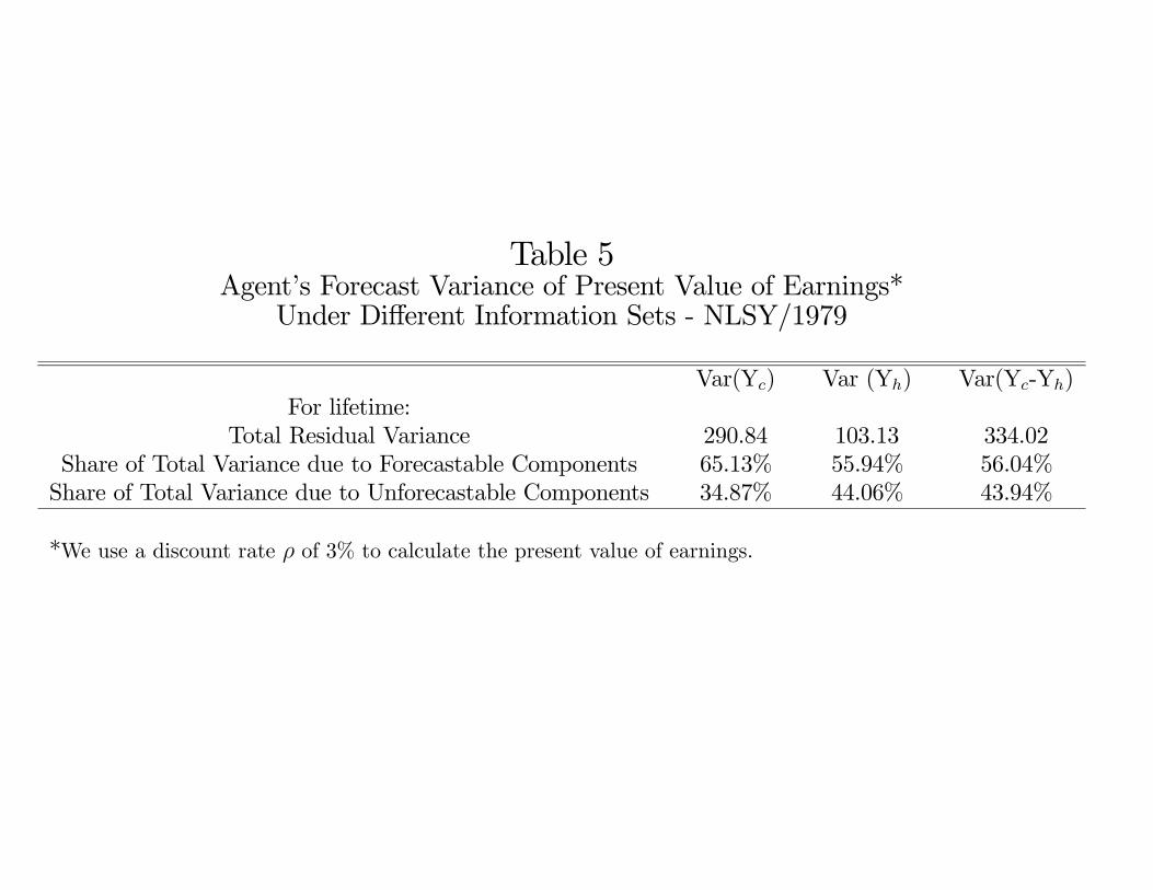
Table 5Agent’s Forecast Variance of Present Value of Earnings*

Under Di erent Information Sets - NLSY/1979

Var(Y ) Var (Y ) Var(Y -Y )For lifetime:

Total Residual Variance 290.84 103.13 334.02Share of Total Variance due to Forecastable Components 65.13% 55.94% 56.04%Share of Total Variance due to Unforecastable Components 34.87% 44.06% 43.94%

*We use a discount rate of 3% to calculate the present value of earnings.

0 50 100 150 200 250 3000

0.005

0.01

0.015

0.02

0.025

Ten Thousand Dollars

FactualCounterfactual

Figure 1Densities of present value of lifetime earnings for High School Graduates

Factual and Counterfactual NLSY/1979 Sample

Present Value of Lifetime Earnings from age 18 to 65 for high school graduates usinga discount rate of 3%. Let Y0 denote present value of earnings in high school sector. LetY1 denote present value of earnings in college sector. In this graph we plot the factualdensity function f(y0 | S=0) (the solid line), against the counterfactual density functionf(y1 | S=0). We use kernel density estimation to smooth these functions.

0 50 100 150 200 250 3000

0.005

0.01

0.015

0.02

0.025

Ten Thousand Dollars

FactualCounterfactual

Figure 2Densities of present value of earnings for College Graduates

Factual and Counterfactual NLSY/1979 Sample

Present Value of Lifetime Earnings from age 18 to 65 for high school graduates usinga discount rate of 3%. Let Y0 denote present value of earnings in high school sector. LetY1 denote present value of earnings in college sector. In this graph we plot the counterfactualdensity function f(y1 | S=0) (the dashed line), against the factual density functionf(y1 | S=0). We use kernel density estimation to smooth these functions.

3 2 1 0 1 2 3 4 50

0.2

0.4

0.6

0.8

1

1.2

1.4

Figure 3Densities of Returns to College

NLSY/1979 Sample

Percent

High School GraduatesCollege Graduates

Let Y0 denote present value of earnings in high school sector. Let Y1 denote present valueof earnings in college sector. Let R = (Y1 - Y0)/Y0 denote the gross rate of return to college.In this graph we plot the density function of the returns to college conditional on being a highschool graduate, f(r | S=0) (the solid line), against the density function of returns to collegeconditional on being a college graduate, f(r | S=1). We use kernel density estimation to smooththese functions.

100 50 0 50 100 150 2000

0.005

0.01

0.015

0.02

0.025

0.03

0.035

Ten Thousand Dollars

Θ = ∅Θ = (θ1)Θ = (θ1,θ2)

Figure 4densities of present value of returns - NLSY/1979

under different information sets for the agent calculatedfor the entire population irregardless of schooling choice

Let Θ denote the information set of the agent. Let Y0 denote the present value ofreturns (discounted at a 3% interest rate). Let f(y0|Θ) denote the density of Y0conditional on information set Θ. The solid line plots the density of Y0 when Θ=φ. The dashed line plots the density of Y0 when Θ={θ1}.The dotted and dashed lineplots the density of of Y0 when Θ={θ1,θ2}. The X variables are in the information

set of the agent. The factors θ, when known, are evaluated at their mean, which is zero.

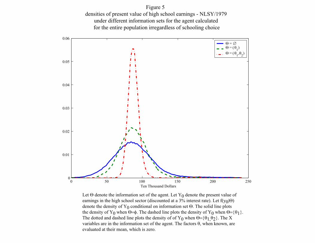
0 50 100 150 200 2500

0.01

0.02

0.03

0.04

0.05

0.06

Ten Thousand Dollars

Θ = ∅Θ = (θ1)Θ = (θ1,θ2)

Figure 5densities of present value of high school earnings - NLSY/1979

under different information sets for the agent calculatedfor the entire population irregardless of schooling choice

Let Θ denote the information set of the agent. Let Y0 denote the present value ofearnings in the high school sector (discounted at a 3% interest rate). Let f(y0|Θ)denote the density of Y0 conditional on information set Θ. The solid line plotsthe density of Y0 when Θ=φ. The dashed line plots the density of Y0 when Θ={θ1}.The dotted and dashed line plots the density of of Y0 when Θ={θ1,θ2}. The Xvariables are in the information set of the agent. The factors θ, when known, areevaluated at their mean, which is zero.

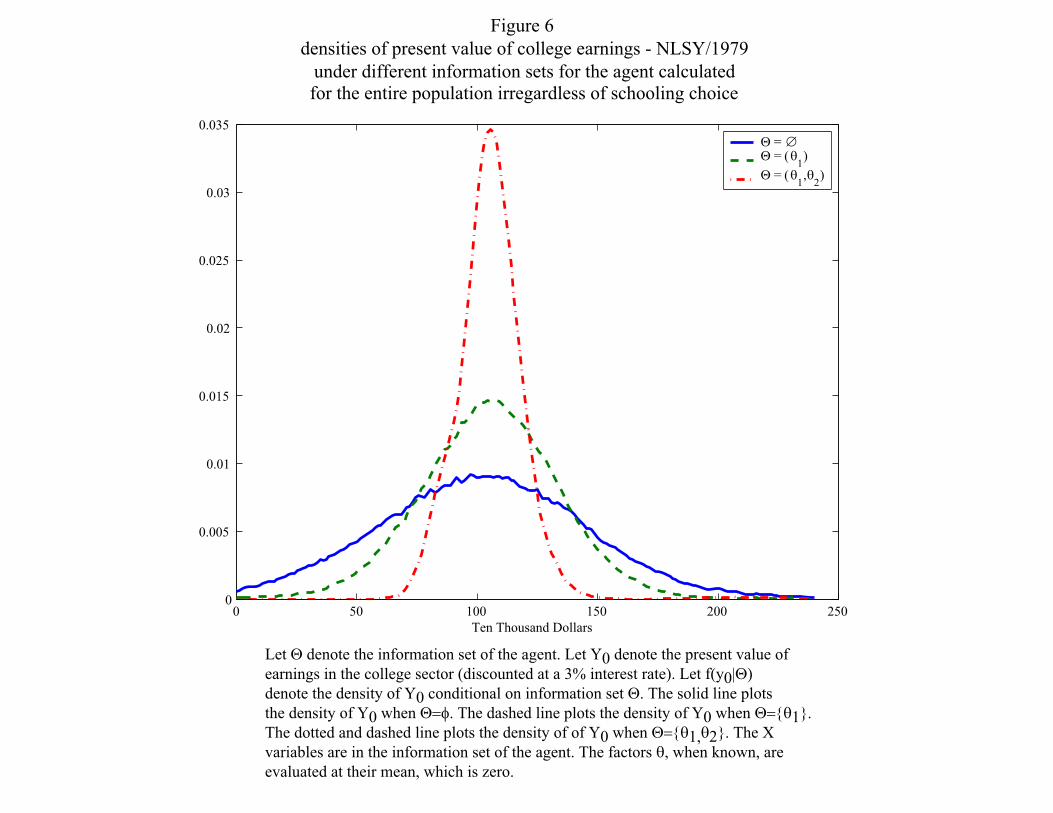
0 50 100 150 200 2500

0.005

0.01

0.015

0.02

0.025

0.03

0.035

Ten Thousand Dollars

Θ = ∅Θ = (θ1)Θ = (θ1,θ2)

Figure 6densities of present value of college earnings - NLSY/1979

under different information sets for the agent calculatedfor the entire population irregardless of schooling choice

Let Θ denote the information set of the agent. Let Y0 denote the present value ofearnings in the college sector (discounted at a 3% interest rate). Let f(y0|Θ)denote the density of Y0 conditional on information set Θ. The solid line plotsthe density of Y0 when Θ=φ. The dashed line plots the density of Y0 when Θ={θ1}.The dotted and dashed line plots the density of of Y0 when Θ={θ1,θ2}. The Xvariables are in the information set of the agent. The factors θ, when known, areevaluated at their mean, which is zero.