Evolutionary Feature and Parameter Selection inSupport Vector Regression

Ivan Mejıa-Guevara1 and Angel Kuri-Morales2

1 Instituto de Investigaciones en Matematicas Aplicadas y Sistemas (IIMAS),Universidad Nacional Autonoma de Mexico (UNAM),

Circuito Escolar S/N, CU, 04510 D. F., Mexicoimejia@uxmcc2.iimas.unam.mx

2 Departamento de Computacion, Instituto Tecnologico Autonomo de Mexico,Rıo Hondo No. 1, 01000 D. F., Mexico

akuri@itam.mx

Abstract. A genetic approach is presented in this article to deal withtwo problems: a) feature selection and b) the determination of parame-ters in Support Vector Regression (SVR). We consider a kind of geneticalgorithm (GA) in which the probabilities of mutation and crossover aredetermined in the evolutionary process. Some empirical experiments aremade to measure the efficiency of this algorithm against two frequentlyused approaches.

Keywords: Support Vector Regression, Self-Adaptive Genetic Algo-rithm, Feature Selection.

1 Introduction

Support Vector Machines (SVMs) have been extensively used as a classificationand regression tool with a great deal of success in practical applications [1] [2][3]. Some of the advantages of SVMs over other traditional methods (as NeuralNetworks) are: a) The development of sound theory first, then implementationand experimentation, b) The solution to an SVM is global and unique, c) Theyhave a simple geometric interpretation and yield a sparse solution, d) The com-putational complexity of SVMs does not depend on the dimensionality of theinput space, e) SVMs take advantage of structural risk minimization and f) Theyare less prone to overfitting [4] [5]. The calibration of parameters for a SVM is animportant aspect to be considered since its learning and generalization capacitydepends on their proper especification [6]. In this article, we focus on the problemof nonlinear regression and we propose a genetic approach for the optimizationof those parameters. The method that we propose also considers the solution tothe problem of feature selection and has the property to be self-adaptive sincethe probabilities of crossover and mutation are determined in the evolutionaryprocess.

A. Gelbukh and A.F. Kuri Morales (Eds.): MICAI 2007, LNAI 4827, pp. 399–408, 2007.c© Springer-Verlag Berlin Heidelberg 2007

400 I. Mejıa-Guevara and A. Kuri-Morales

The article is organized as follows. We discuss in section 2 some theoreticalcharacteristics of SVR. In section 3, we describe a self-adaptive Genetic Algo-rithm approach. In section 4 we describe some experiments where other ap-proaches are used to solve the problem of determining the proper selection ofparameters in SVR and the results obtained from comparisons performed againstthese approaches. Finally, some conclusions are presented.

2 Support Vector Regression

SVM is a supervised method discovered by Vapnik et al [7] and has been ex-tensiveley used in the solution of pattern classification, nonlinear regression andother problems. In this section we focus on the problem of regression, where aset of data (the training dataset) τ = {xi, yi}N

i=1, is considered for the train-ing process, where yi, i = 1, . . . , N are continuous output values. Given thistraining set, the goal of SVR is to approximate a linear function of the formf(x) = 〈w, x〉+ b with w ∈ RN and b ∈ R that minimizes an empirical risk func-tion defined by Remp = 1

N

∑Ni=1 Lε (y − f(x)), where Lε (y − f(x)) = |ξ| − ε, if

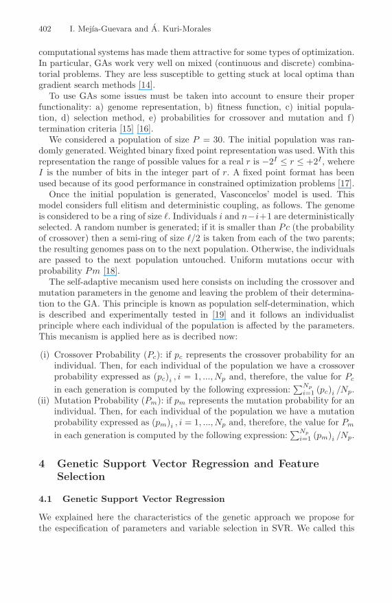
|ξ| > ε and 0 in other case. The term ξ is called slack variable and is introducedto cope with otherwise infeasible constraints of the optimization problem [8]. Inother words, errors are disregarded as long as they are smaller than a properlyselected ε as shown is Figure 1.a). The last function is called epsilon-insensitiveloss function, but it is important to point out that it is posible to use otherkinds of loss functions in SVR. In Figure 1.b) a graphical representation of it ispresented. In order to estimate f(x) a quadratic problem must be solved, which

Fig. 1. (a) Nonlinear Regression Function and penalization of points beyond limits ofthe ε-tube, (b) ε-Insensitive Loss Function

has the objective to minimize the empirical risk function. The dual form of thisoptimization problem is more appropriate. This formulation is as follows:

Maxα,α∗ −12

N∑

i=1

N∑

j=1

(αi − α∗i )

(αj − α∗

j

)K (xi, xj)

Evolutionary Feature and Parameter Selection in Support Vector Regression 401

−ε

N∑

i=1

(αi + α∗i ) +

N∑

i=1

yi (αi − α∗i ) (1)

s.t. :N∑

j=1

(αi − α∗i ) = 0

αi, α∗i ∈ [0, C]

The regularization parameter C > 0 determines the tradeoff between the flatnessof f(x) and the allowed number of points with deviations larger than ε. The valueof ε is inversely proportional to the number of support vectors (represented by(αi − α∗

i ) �= 0) [8]. An adequate determination of C and ε is needed for a propersolution of the problem. Some approaches has been proposed in the past for theirdetermination either for the C parameter [9] or for both [10].The determinationof these parameters is the main objective here, so the method we propose isexplained in the next section.

Functional K (xi, xj) in (1) is known a kernel function and it allows to projectthe original problem to a higher dimensional feature space where the datasethas a high probability to be linearly separable. Many functions can be used askernels, but only if they fulfill Mercer’s theorem [11]. Some of the most popularkernels discussed in the literature are the radial basis functions (RBF) (2) andthe polynomial kernel (PK) (3). In this paper we focus on the latter and we usedthem to compare the accuracy of the algorithm that we suggest against the oneobtained with other alternatives. The expressions that characterize these kernelsare as follows:

K (x,xi) = e−‖x−xi‖2

2σ2 (2)K (x,xi) = (1 + x.xi)

ρ (3)

The parameters σ and ρ have to be properly determined in order for the SVMto generalize well. From now on, we refer to these parameters as kernel pameters(kP ), when we use either polynomial or Gaussian kernels in the experiments wewill describe below. The selection of these parameters is very important becausethe kP determines the complexity of the model and affects its accuracy. Forthat reason, different approaches have been proposed in the past for its optimalselection [12] [13]. Their determination is also a very important objective and,therefore, we propose an alternative genetic approach.

Once the solution of (1) is obtained, the support vectors are used to constructthe following regression function:

f (x) =N∑

i=1

(αi − α∗i )K (x, xi) + b (4)

3 Self-adaptive Genetic Algorithm

Genetic Algorithms were formally introduced in the 1970s by John Hollandand his students at the University of Michigan. Their advantage over other

402 I. Mejıa-Guevara and A. Kuri-Morales

computational systems has made them attractive for some types of optimization.In particular, GAs work very well on mixed (continuous and discrete) combina-torial problems. They are less susceptible to getting stuck at local optima thangradient search methods [14].

To use GAs some issues must be taken into account to ensure their properfunctionality: a) genome representation, b) fitness function, c) initial popula-tion, d) selection method, e) probabilities for crossover and mutation and f)termination criteria [15] [16].

We considered a population of size P = 30. The initial population was ran-domly generated. Weighted binary fixed point representation was used. With thisrepresentation the range of possible values for a real r is −2I ≤ r ≤ +2I , wehereI is the number of bits in the integer part of r. A fixed point format has beenused because of its good performance in constrained optimization problems [17].

Once the initial population is generated, Vasconcelos’ model is used. Thismodel considers full elitism and deterministic coupling, as follows. The genomeis considered to be a ring of size �. Individuals i and n−i+1 are deterministicallyselected. A random number is generated; if it is smaller than Pc (the probabilityof crossover) then a semi-ring of size �/2 is taken from each of the two parents;the resulting genomes pass on to the next population. Otherwise, the individualsare passed to the next population untouched. Uniform mutations occur withprobability Pm [18].

The self-adaptive mecanism used here consists on including the crossover andmutation parameters in the genome and leaving the problem of their determina-tion to the GA. This principle is known as population self-determination, whichis described and experimentally tested in [19] and it follows an individualistprinciple where each individual of the population is affected by the parameters.This mecanism is applied here as is decribed now:

(i) Crossover Probability (Pc): if pc represents the crossover probability for anindividual. Then, for each individual of the population we have a crossoverprobability expressed as (pc)i , i = 1, ..., Np and, therefore, the value for Pc

in each generation is computed by the following expression:∑Np

i=1 (pc)i /Np.(ii) Mutation Probability (Pm): if pm represents the mutation probability for an

individual. Then, for each individual of the population we have a mutationprobability expressed as (pm)i , i = 1, ..., Np and, therefore, the value for Pm

in each generation is computed by the following expression:∑Np

i=1 (pm)i /Np.

4 Genetic Support Vector Regression and FeatureSelection

4.1 Genetic Support Vector Regression

We explained here the characteristics of the genetic approach we propose forthe especification of parameters and variable selection in SVR. We called this

Evolutionary Feature and Parameter Selection in Support Vector Regression 403

approximation as Genetic Support Vector Regression (GSVR) and its implemen-tation is as follows:

(1) Define the genome for the representation of the parameters: C, kP , ε, Pc,Pm and fS

(2) Randomly generate the initial population,(3) Compute the fitness for each individual of the population,(4) Apply genetic operations based on Vasconcelo’s method and the self-adaptive

approach,(5) If a termination criterion is reached, finish. If not, return to step 3.

Similar approaches have been used for classification problems in [20] [21], butnew characteristics are considered here that have proven their efficiency in thepast [18]: a) The fixed-point codification, b) The use of an efficient genetic strat-egy (Vasconcelos) and, b) The self-adaptive mecanism where Pc and Pm aredetermined in the evolutionary process.

The parameter fS in the step (1) will be useful for the implementation offeature selection, but the details are explained in the next section. Concerningstep (3), the fitness is defined as the Mean Square Error (MSE), computed afterthe application of Cross-Validation. Other alternative is the estimation of theMSE defined on a test dataset, which is a faster way to compute the error, but astatistical analysis of the application of this approach in classification problemsshowed that the variance is higher [12] and for that reason we decided to use theCross-Validation error.

The MSE is computed for each individual in the population and for the newindividual generated in the evolutionary process through the application of theSequential Minimal Optimization (SMO) algorithm, which is an efficient and fastway to train SVMs for classification and regression problems. The algorithm forclassification was discovered by Platt [22] and an efficient algorithm for regressiontraining with SMO is due to [23]. The kind of algorithm that is chosen in thisphase is very important since most of the training time depends on its selection.The use of traditional optimization methods here is out of the question, becauseof the time these algorithms could need for training. Therefore, altough someother algorithms can be used for training the SVM, we strongly suggest the useof the SMO approach.

Finally, step (5) refers to the stopping criterion for the GA. The one thatwe used is based on the number of generations, where only 50 generations wereneeded to obtain a competitive machine. For instance, in [20] the stopping crite-ria was 600 generations or that the fitness value does not improve during the last100 generations. Moreover, 500 individual were used in that application in com-parison with the 30 individual we use here. Those differences imply a significantdecrease on the computation cost as we show in our experiments.

4.2 Feature Selection

A problem that has been a matter of study for many years is the selection of asubset of relevant variables for building robust learning methods. The terminology

404 I. Mejıa-Guevara and A. Kuri-Morales

of variable selection, feature reduction, attribute selection or variable subset areequivalent ways used in the literature when refering to this problem. The objectiveof variable selection is three-fold: a) improving the prediction performance of amachine learning, b) providing faster and more cost-effective predictors, and c)providing a better understanding of the underlying process that generated the data[24]. The evolutionary procedure used here consists of introducing a binary stringof size equal to the number of independent variables of τ , where a ′0′ in positioni means that the variable i must be dropped during the training process and a ′1′

means the opposite. For instance, if the problem in question has 7 variables, thestring 0101011means that only the variables 2, 4, 6 and 7 must be used for training.

Once all the variables that will be especified in the genome have been definedthe size of the genome for the GSVR is equal to nC + nkp + nε + npc + npm + m,where nC , nkp, nε, npc, npm and m are the number of bits used for the codificationof C, kP , ε, Pc, Pm and the number of characteristics, respectiveley.

Given the elitism property of the Vasconcelos’ GA, the problem of sacrificingfitness when some variables of the training set are not considered is avoided sincethe evolutionary process begins with all variables, but a reduced subset of thosevariables is always kept.

5 Experiments and Results

In this section we use the genetic approach explained before for the determinationof parameters in SVMs applied in the solution of nonlinear regression problems.To prove the efficiency of this method we compare its results against other twoapproaches used in the past for similar purposes. The first method is due toCherkassky (CHK) et al [10], who proposed an analytical calculation of C andε. The other approach consists of the use of Cross Validation (CV), which allowsthe calibration of C, ε and the kernel parameter.

The CHK method suggests the use of C = max (|y + 3σy| , |y − 3σy|) for theestimation of C, where y and σy are the mean and standard deviation of the out-put values of the training set, respectively. The last expression is applicable whena radial basis kernel function is used and it is derived taking into account the re-gression function (4) and the constraints in (1), where the support vectors and Care involved. The evaluation of ε is reached computing ε ∝ σ√

n, where σ is the

noise deviation of the problem. However, this methodology is only applicable forlow values of N , since higher ones imply a very low ε. Given this drawback, the au-

thor recommends the use of ε = τσ√

lnNN instead, τ being a constantwhichmust be

empirically determined and σ is calculated in practice using the following equation:

σ =1

n − d

N∑

i=1

(y − y)2 (5)

where y is the estimated output value gotten from the application of high orderpolynomials1. We use Minimax Polynomial Approximation (MPA) to deal with1 The author also suggests other approach, but we use this one.

Evolutionary Feature and Parameter Selection in Support Vector Regression 405

this problem. It is important to mention that with this technique it is not possibleto estimate kP and this is done here by using some arbitary values and applyingCross-Validation once the proper values of C and ε had been estimated.

The Cross-Validation alternative is applied for the selection of parameters bychoosing -arbitrarily or randomly- some values for each parameter. The propervalues are chosen as the ones with the lowest CV error, where k-fold or Leave-one-Out (LoO) Cross Validation are very common in practice.

The datasets used for the comparison of the three methods were taken from theUniversity of California at Irving Machine Learning Repository2 (UMLR) whichare labeled as mpg, mg and diabetes. The first dataset refers to the problemof predicting the efficiency in fuel consumption for several kinds of car models,it consists of 7 characteristics and 392 observations. The second problem has1385 points with 6 independent variables each [23]. The third one concerns thestudy of the factors affecting patterns of insulin-dependent diabetes mellitusin children and it has 43 observations with 2 continuous characteristics3. Wecalculated the MSE for each experiment after applying 5-fold Cross-Validation.We also computed the execution time using a 1.8 MH Intel-Centrino processorwith 512 RAM memory.

Two kernel functions were used during these experiments: a kernel functionand a radial Gaussian basis function. As mentioned before, the parameters forthese kernels were genetically calibrated for the GSVR approach and using 5-foldCV in every case.

MSEs, parameter values and execution times for each algorithm are shown inTable 14 (The label GSVR-RBF stands for Genetic Support Vector Regressiontrained with a RBF and so on.)

According with the results in Table 1, we can appreciate that GSVR approachis very competitive in comparison with the other methods. MSEs in the geneticmethod were at almost the same or lower than the ones obtained with CHKmethod, but the execution time was better. However, the most important ad-vantage of GSVR is that it is of more general application because of its flexibilityin the use of other kinds of kernel function in the trainning process. This is notposible with the CHK method.

Performance of the CV method is not conlcusive in comparison with GSVRbecause it is worse than the one for diabetes, the same for mg and better formpg for the two kinds of kernels, besides the performance of GSVR with apolynomial kernel is slightly better than the performance with RBF kernel. Theproblem with CV is the computation time, because it is significatly larger thanthe computation in GSVR for mpg and mg. The time for CV is almost 8 timeslarger than GSVR computation time in mpg with 30 individuals and 50 genera-tions, using a RBF and almost twice using the polynomial kernel. In the case of2 http://mlearn.ics.uci.edu/MLRepository.html3 This data can be downloaded from:

http://www.liacc.up.pt/ ltorgo/Regression/DataSets.html4 The time for CHK depends on the algorithm that is used for the estimation of σ

and, for that reason, it is not reported in this Table. However, this time was similaror smaller than the one spent on the other approaches.

406 I. Mejıa-Guevara and A. Kuri-Morales

Table 1. MSE, time (in minutes) and parameters estimated with CHK method, CVmethod and GSVR, using RBF and PK

Problems Time MSE C ε kPmpg

GSVR-RBF 6.22 6.59 15.85 0.31 0.53GSVR-PK 48.07 7.16 4.40 0.46 3CV-RBF 46.64 6.81 13.34 0.84 0.5CV-PK 92.71 7.17 43.49 0.84 3CHK 7.17 46.86 0.47 0.5

diabetesGSVR-RBF 1.38 0.32 14.97 0.49 0.2145GSVR-PK 1.32 0.31 1.23 0.49 2CV-RBF 1.53 0.28 5.56 0.68 0.5CV-PK 0.87 0.28 5.56 0.70 2CHK 0.34 6.91 0.51 0.5

mg

GSVR-RBF 28.23 0.01 2.44 0.09 3.6602GSVR-PK 847.80 0.02 30.91 0.10 3VC-RBF 120.02 0.01 0.09 0.06 1.1VC-PK 939.00 0.02 8.77 0.01 3CHK 0.02 1.61 0.05 0.8

diabetes, the time for both methods is almost the same, maybe because the num-ber of observations for this dataset is the smallest (the difference is no greaterthan 0.5 minutes for the entire training and optimization). In mg, the compu-tation time is 4 times larger for CV with a RBF and 50 minutes larger withthe polynomial kernel. Other problem with CV is the selection of candidates asoptimal parameters in the process of optimization. Even when this operation isdone randomly, the range of the values for those parameters in not clear. More-over, just a limited number of values for those parameters can be chosen withthis technique. With the GSVR method, on the other hand, the problem of therange is similar but there are more possibilities.

Feature selection is other important characteristic of the GSVR and it is alsoanother advantage since CHK method does not consider how to tackle this prob-lem and CV method could be applied in [25] but with a significant aditional com-putation cost, which actually is its main disadvantage as we mentioned before.

6 Conclusions

A new algorithm was presented in this article to tackle the problem of feature se-lection and the calibration of parameters in SVR. The proposed method, namedGSVR, was superior in comparison with two approaches used in the past forseveral reasons: a) the fitness of GSVR was the same or better in the majority ofcases, b) the computation time is significantly smaller than the time CV takes

Evolutionary Feature and Parameter Selection in Support Vector Regression 407

for the same problems, c) the GSVR is most robust than Cherkassky approachsince it can be applied in principle with many different kinds of kernel functionsand, d) feature selection is implemented with GSVR with no additional com-putational cost and without loss in accuaracy. A robust methodology for thestatistical validation of different machine learning methods designed for tacklingnonlinear regression problems is a matter of future work.

References

1. Guyon, W., Barnhill, V.: Gene selection for cancer classification using supportvector machines. MACHLEARN: Machine Learning 46 (2002)

2. Huang, Z., Chen, H., Hsu, C.J., Chen, W.H., Wu, S.: Credit rating analysis withsupport vector machines and neural networks: a market comparative study. Deci-sion Support Systems 37(4), 543–558 (2004)

3. Kim, K.J.: Financial time series forecasting using support vector machines. Neu-rocomputing 55(1-2), 307–319 (2003)

4. Burges, C.J.C.: A tutorial on support vector machines for pattern recognition. DataMining and Knowledge Discovery 2(2), 121–167 (1998)

5. Cristianini, N., Shawe-Taylor, J.: An Introduction to Support Vector Machines andOther Kernel-Based Learning Methods. Cambridge University Press, Cambridge(2000)

6. Chapelle, O., Vapnik, V., Bousquet, O., Mukherjee, S.: Choosing multiple param-eters for support vector machines. Machine Learning 46(1/3), 131 (2002)

7. Boser, B.E., Guyon, I., Vapnik, V.: A training algorithm for optimal margin clas-sifiers. In: COLT, pp. 144–152 (1992)

8. Smola, A., Scholkopf, B.: A tutorial on support vector regression (2004)9. Kuri-Morales, A., Mejıa-Guevara, I.: Evolutionary training of svm for multiple

category classification problems with self-adaptive parameters. In: Simao-Sichman,J., Coelho, H., Oliveira-Rezende, S. (eds.) IBERAMIA/SBIA 2006. LNCS (LNAI),pp. 329–338. Springer, Heidelberg (2006)

10. Cherkassky, V., Ma, Y.: Practical selection of SVM parameters and noise estimationfor SVM regression. Neural Networks 17(1), 113–126 (2004)

11. Haykin, S.: Neural networks: A comprehensive foundation. MacMillan, New York(1994)

12. Mejıa-Guevara, I., Kuri-Morales, A.: Genetic support vector classification and min-imax polynomial approximation (2007),http://www.geocities.com/gauss75/ivan.html

13. Friedrichs, F., Igel, C.: Evolutionary tuning of multiple svm parameters. Neuro-computing 64, 107–117 (2005)

14. Holland, J.H.: Adaptation in natural artificial systems. University of MichiganPress, Ann Arbor (1975)

15. Goldberg, D.E.: Genetic Algorithms in Search, Optimization and Machine Learn-ing. Addison-Wesley, Reading (1989)

16. Mitchell, M.: An Introduction to Genetic Algorithms. MIT Press, Cambridge(1996)

17. Kuri, A.: A Comprehensive Approach to Genetic Algorithms in Optimization, andLearning. Theory and Applications, Foundations. vol. 1. IPN (1999)

18. Kuri-Morales, A.F.: A methodology for the statistical characterization of geneticalgorithms. In: Coello Coello, C.A., de Albornoz, A., Sucar, L.E., Battistutti, O.C.(eds.) MICAI 2002. LNCS (LNAI), vol. 2313, Springer, Heidelberg (2002)

408 I. Mejıa-Guevara and A. Kuri-Morales

19. Galaviz, J., Kuri, A.: A self-adaptive genetic algorithm for function optimization.In: ISAI/IFIPS, p. 156 (1996)

20. Huang, C.L., Wang, C.J.: A ga-based feature selection and parameters optimizationfor support vector machines. Expert Syst. Appl. 31(2), 231–240 (2006)

21. Min, S.H., Lee, J., Han, I.: Hybrid genetic algorithms and support vector machinesfor bankruptcy prediction. Expert Syst. Appl. 31(3), 652–660 (2006)

22. Platt, J.: Fast training of support vector machines using sequential minimal opti-mization. In: Scholkopf, B., Burges, C.J.C., Smola, A.J. (eds.) Advances in KernelMethods — Support Vector Learning, pp. 185–208. MIT Press, Cambridge (1999)

23. Flake, G.W., Lawrence, S.: Efficient svm regression training with smo. MachineLearning (2001)

24. Guyon, I., Elisseeff, A.: An introduction to variable and feature selection. Journalof Machine Learning Research 3, 1157–1182 (2003)

25. Abe, S.: Modified backward feature selection by cross validation. In: ESANN, pp.163–168 (2005)