Clim. Past, 7, 1139–1148, 2011www.clim-past.net/7/1139/2011/doi:10.5194/cp-7-1139-2011© Author(s) 2011. CC Attribution 3.0 License.

Climateof the Past

Evolution of the seasonal temperature cycle in a transient Holocenesimulation: orbital forcing and sea-ice

N. Fischer1,2 and J. H. Jungclaus1

1Max Planck Institute for Meteorology, Hamburg, Germany2International Max Planck Research School for Earth System Modelling, Hamburg, Germany

Received: 19 January 2011 – Published in Clim. Past Discuss.: 3 February 2011Revised: 14 September 2011 – Accepted: 28 September 2011 – Published: 8 November 2011

Abstract. Changes in the Earth’s orbit lead to changesin the seasonal and meridional distribution of insolation.We quantify the influence of orbitally induced changeson the seasonal temperature cycle in a transient simula-tion of the last 6000 years – from the mid-Holocene to to-day – using a coupled atmosphere-ocean general circulationmodel (ECHAM5/MPI-OM) including a land surface model(JSBACH).

The seasonal temperature cycle responds directly to the in-solation changes almost everywhere. In the Northern Hemi-sphere, its amplitude decreases according to an increase inwinter insolation and a decrease in summer insolation. In theSouthern Hemisphere, the opposite is true.

Over the Arctic Ocean, decreasing summer insolationleads to an increase in sea-ice cover. The insulating effectof sea ice between the ocean and the atmosphere leads todecreasing heat flux and favors more “continental” condi-tions over the Arctic Ocean in winter, resulting in stronglydecreasing temperatures. Consequently, there are two com-peting effects: the direct response to insolation changes anda sea-ice insulation effect. The sea-ice insulation effect isstronger, and thus an increase in the amplitude of the sea-sonal temperature cycle over the Arctic Ocean occurs. Thisincrease is strongest over the Barents Shelf and influencesthe temperature response over northern Europe.

We compare our modeled seasonal temperatures over Eu-rope to paleo reconstructions. We find better agreements inwinter temperatures than in summer temperatures and better

Correspondence to:N. Fischer(nils.fischer@zmaw.de)

agreements in northern Europe than in southern Europe,since the model does not reproduce the southern EuropeanHolocene summer cooling inferred from the paleo recon-structions. The temperature reconstructions for northern Eu-rope support the notion of the influence of the sea-ice insula-tion effect on the evolution of the seasonal temperature cycle.

1 Introduction

The amplitude of the seasonal temperature cycle dependson changes in the Earth’s orbital parameters that alter theseasonal and the meridional distribution of insolation (Mi-lankovic, 1941; Berger, 1978). The orbital forcing consti-tutes the dominant natural long-term climate forcing in thelast 6000 yr, from the mid-Holocene to today (e.g.,Wanneret al., 2008; Renssen et al., 2009). The Earth’s obliquity waslarger 6000 yr ago and, at the same time, summer solsticewas closer to perihelion. In the Northern Hemisphere, this re-sulted in higher insolation in summer and lower insolation inwinter, and, consequently, in increased seasonal differencesin insolation. So far, it has been assumed that this increase ininsolation seasonality has also lead to increased surface tem-perature seasonality. If this is the case for all latitudes, or ifresponses of the climate system to insolation changes have tobe taken into account is subject of the present study.

The insolation changes act on millennial time-scales andare due to the precession of the Earth’s elliptical orbit aroundthe Sun and the changes in obliquity of the Earth’s rota-tion axis with respect to the orbital plane. Annual meanchanges in insolation – driven by obliquity changes – wererelatively small (<4.5 W m−2 at high latitudes) compared to

Published by Copernicus Publications on behalf of the European Geosciences Union.

1140 N. Fischer and J. H. Jungclaus: Holocene seasonal cycle

the seasonal insolation changes (up to more than 30 W m−2

for June insolation at high latitudes). Feedbacks between thedifferent components of the Earth’s system, e.g., the sea-ice-albedo feedback, have the potential to amplify or dampenthe insolation signal. These feedbacks act in different sea-sons and the annual temperature change is the sum of theseasonal temperature changes that vary in their individualamplitudes. Therefore, the annual signal can be dominatedby one particular season, and hence, by seasonality. Thisleads to changes in climate also on time-scales longer thanseasonal as has been shown in several time-slice simulationstudies (e.g.,Braconnot et al., 2007a; Otto et al., 2009).

Denton et al.(2005) discuss the role of seasonality inabrupt climate change events during the last 60 000 yr bymeans of temperature reconstructions from ice cores andglacier advances in Greenland. The authors find that duringabrupt cold climate events, the annual temperature anomaliesin high northern latitudes are dominated by the winter tem-perature anomalies that are caused by increased winter sea-ice cover in the Northern Hemisphere. This leads to “conti-nental” conditions over large parts of the northern high lati-tudes and thus to an increase in the amplitude of the seasonaltemperature cycle.

Previous large-scale proxy-based studies that analyzedHolocene summer and winter temperatures consist of com-pilations of local climate reconstructions and are mainly fo-cused on the mid-Holocene (6 ka) because of different datingprocedures and different temporal resolutions of the individ-ual reconstructed temperature time-series.Cheddadi et al.(1996) find higher summer and winter temperatures in north-ern European high latitudes and lower winter and summertemperatures in the Mediterranean region. Similar resultsfor high and lower Northern Hemisphere latitudes are foundfor Siberia (Tarasov et al., 1999) and in a more recent sur-vey, on high northern latitude temperatures bySundqvistet al. (2010). There is qualitative agreement between thetime-slice studies and the evolution of seasonal temperaturesthroughout the Holocene over Europe, presented inDaviset al. (2003). The results of this study are compared to oursimulation results later in the present study.

Time-slice simulations of the mid-Holocene with coupledAO-GCMs have been part of the PMIP2-initiative (e.g.,Bra-connot et al., 2007a,b) that covered various aspects of theclimate system but did not investigate the response of the sea-sonal temperature cycle to changes in insolation. The sameis true for transient simulations of the Holocene performedwith either Earth system models of intermediate complexity(e.g.,Renssen et al., 2009) or transient Holocene simulationswith AO-GCMs simulations and accelerated orbital forcing(Lorenz et al., 2006).

Transient simulations allow us to check whether the cli-mate model exhibits any non-linear responses to the appliedorbital forcing. These responses have been found, e.g., inlow latitude vegetation in previous studies on Holocene cli-mate studies (e.g.,Claussen et al., 1999; Liu et al., 2006).

A further advantage of transient simulations is the improvedcomparability of the model results to reconstructions frompaleo-climate-proxies. Climate models tend to have biases incertain simulated quantities and also reconstructed data haveuncertainties. Transient simulations enable us to compare thetrends in the climate variable and therefore allow for a morerobust assessment of temporal changes in the climate system.

In this study, we investigate how changes in insolation af-fect the mean climate evolution and the evolution of the sea-sonal cycle from the mid-Holocene to today. Given the sea-sonal distribution of insolation in the Northern Hemispherein the mid-Holocene, the expected direct respone is a de-crease in the amplitude of the seasonal temperature cycle inthe course of the last 6000 yr. Nevertheless, sea-ice evolu-tion over the Arctic Ocean and the interaction between at-mosphere, ocean, and sea ice may alter this direct response.In the first part of this study, we present the evolution of theseasonal temperature cycle over the last 6000 yr in a cou-pled atmosphere-ocean model with an integrated dynamicland surface model. In the second part, we compare the sim-ulation results to Holocene temperature reconstructions ob-tained from pollen archives.

2 Model setup and experimental design

We perform a 6000-year-long transient simulation withthe coupled atmosphere-ocean general circulation modelECHAM5/MPI-OM (Jungclaus et al., 2006), including theland surface model JSBACH (Raddatz et al., 2007) witha dynamic vegetation module (Brovkin et al., 2009) ac-counting for vegetation induced changes in surface prop-erties. The atmosphere component ECHAM5 (Roeckneret al., 2003) is run in resolution T31 (corresponding to 3.75◦)and the ocean component MPI-OM (Marsland et al., 2003)is run in resolution GR30 (corresponding to∼3◦). Theocean model component includes a Hibler-type zero-layerdynamic-thermodynamic sea-ice model with viscous-plasticrheology (Semtner, 1976; Hibler, 1979).

Since we are mainly interested in the effects of orbitalforcing on the evolution of the seasonal temperature cycle,we do not apply further external forcing such as solar, vol-canic, or greenhouse gases and set greenhouse gas concen-trations to pre-industrial values (CO2 to 280 ppm, CH4 to700 ppb, N2O to 265 ppb). Thus, we do not expect the modelresults to perfectly match climate reconstructions. Rather,we are interested in finding mechanisms that determine thechanges in the seasonal temperature cycle from the mid-Holocene to today. We apply orbital forcing on a yearly ba-sis following (Bretagnon and Francou, 1988) implementedin the radiation scheme of the atmosphere model component,which are similar to other calculations of insolation change(e.g.,Berger, 1978). We do not apply any acceleration tech-nique and can thus analyze the ocean’s response to changesin insolation on orbital timescales. We initialize the transient

Clim. Past, 7, 1139–1148, 2011 www.clim-past.net/7/1139/2011/

N. Fischer and J. H. Jungclaus: Holocene seasonal cycle 1141

experiment from a 3500-year-long mid-Holocene (6000 yrbefore present) time-slice simulation with orbital forcing pre-sented in an earlier study (Fischer and Jungclaus, 2010).

3 Results and discussion

For the following analysis, we use monthly mean output fromboth the atmosphere and the ocean model with the standardpresent-day calendar. The time-period of reference is themid-Holocene, i.e., 6000 yr before present.

3.1 Seasonal insolation and sea-ice effects

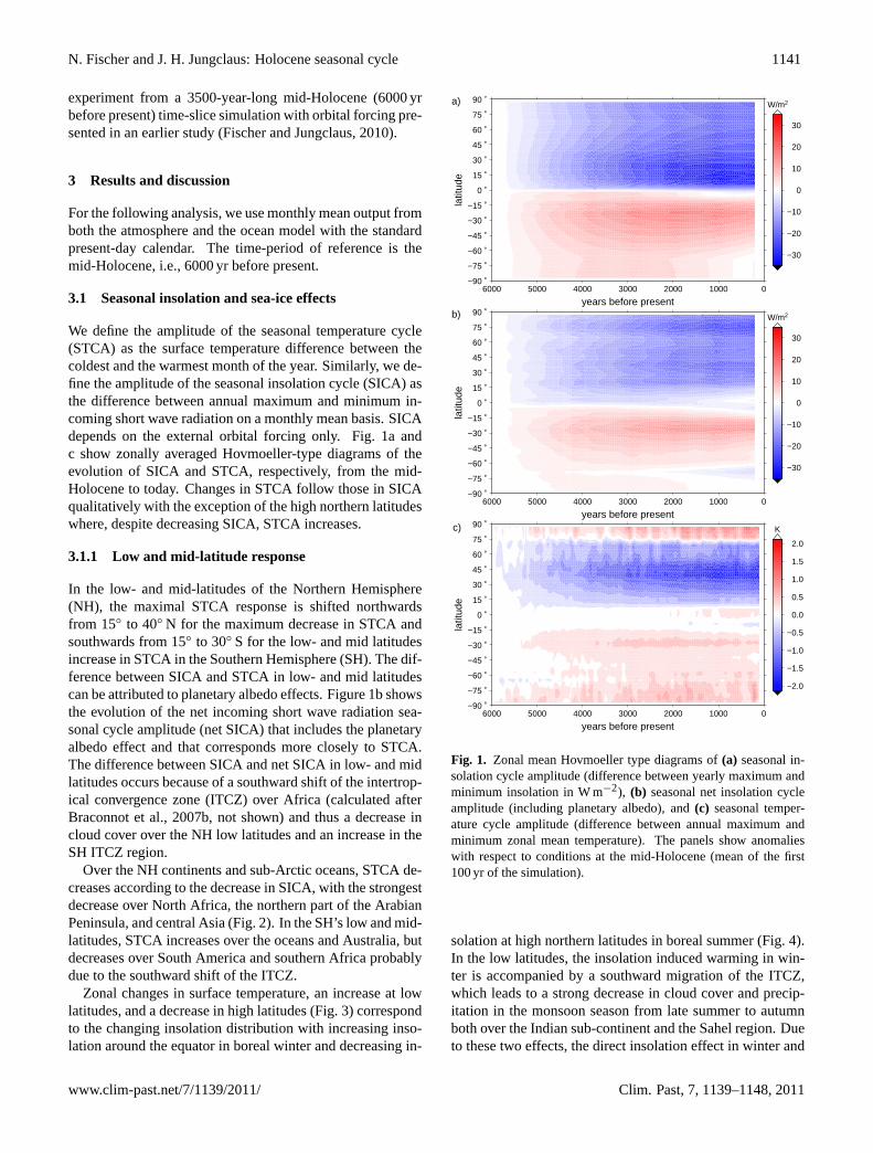
We define the amplitude of the seasonal temperature cycle(STCA) as the surface temperature difference between thecoldest and the warmest month of the year. Similarly, we de-fine the amplitude of the seasonal insolation cycle (SICA) asthe difference between annual maximum and minimum in-coming short wave radiation on a monthly mean basis. SICAdepends on the external orbital forcing only. Fig.1a andc show zonally averaged Hovmoeller-type diagrams of theevolution of SICA and STCA, respectively, from the mid-Holocene to today. Changes in STCA follow those in SICAqualitatively with the exception of the high northern latitudeswhere, despite decreasing SICA, STCA increases.

3.1.1 Low and mid-latitude response

In the low- and mid-latitudes of the Northern Hemisphere(NH), the maximal STCA response is shifted northwardsfrom 15◦ to 40◦ N for the maximum decrease in STCA andsouthwards from 15◦ to 30◦ S for the low- and mid latitudesincrease in STCA in the Southern Hemisphere (SH). The dif-ference between SICA and STCA in low- and mid latitudescan be attributed to planetary albedo effects. Figure1b showsthe evolution of the net incoming short wave radiation sea-sonal cycle amplitude (net SICA) that includes the planetaryalbedo effect and that corresponds more closely to STCA.The difference between SICA and net SICA in low- and midlatitudes occurs because of a southward shift of the intertrop-ical convergence zone (ITCZ) over Africa (calculated afterBraconnot et al., 2007b, not shown) and thus a decrease incloud cover over the NH low latitudes and an increase in theSH ITCZ region.

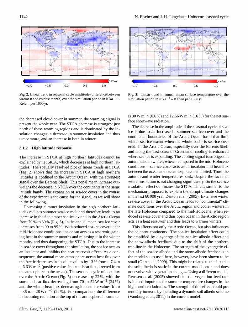
Over the NH continents and sub-Arctic oceans, STCA de-creases according to the decrease in SICA, with the strongestdecrease over North Africa, the northern part of the ArabianPeninsula, and central Asia (Fig.2). In the SH’s low and mid-latitudes, STCA increases over the oceans and Australia, butdecreases over South America and southern Africa probablydue to the southward shift of the ITCZ.

Zonal changes in surface temperature, an increase at lowlatitudes, and a decrease in high latitudes (Fig.3) correspondto the changing insolation distribution with increasing inso-lation around the equator in boreal winter and decreasing in-

−90 ˚

−75 ˚

−60 ˚

−45 ˚

−30 ˚

−15 ˚

0 ˚

15 ˚

30 ˚

45 ˚

60 ˚

75 ˚

90 ˚

latit

ude

0100020003000400050006000

years before present

−30

−20

−10

0

10

20

30

W/m2

−90 ˚

−75 ˚

−60 ˚

−45 ˚

−30 ˚

−15 ˚

0 ˚

15 ˚

30 ˚

45 ˚

60 ˚

75 ˚

90 ˚

latit

ude

0100020003000400050006000

years before present

−2.0

−1.5

−1.0

−0.5

0.0

0.5

1.0

1.5

2.0

K

−90 ˚

−75 ˚

−60 ˚

−45 ˚

−30 ˚

−15 ˚

0 ˚

15 ˚

30 ˚

45 ˚

60 ˚

75 ˚

90 ˚

latit

ude

0100020003000400050006000

years before present

−30

−20

−10

0

10

20

30

W/m2a)

b)

c)

Fig. 1. Zonal mean Hovmoeller type diagrams of a) seasonal insolation cycle amplitude (difference between

yearly maximum and minimum insolation in W/m2), b) seasonal net insolation cycle amplitude (including plan-

etary albedo), and c) seasonal temperature cycle amplitude(difference between annual maximum and minimum

zonal mean temperature). The panels show anomalies with respect to conditions at the mid-Holocene (mean of

the first 100 years of the simulation).

13

Fig. 1. Zonal mean Hovmoeller type diagrams of(a) seasonal in-solation cycle amplitude (difference between yearly maximum andminimum insolation in W m−2), (b) seasonal net insolation cycleamplitude (including planetary albedo), and(c) seasonal temper-ature cycle amplitude (difference between annual maximum andminimum zonal mean temperature). The panels show anomalieswith respect to conditions at the mid-Holocene (mean of the first100 yr of the simulation).

solation at high northern latitudes in boreal summer (Fig.4).In the low latitudes, the insolation induced warming in win-ter is accompanied by a southward migration of the ITCZ,which leads to a strong decrease in cloud cover and precip-itation in the monsoon season from late summer to autumnboth over the Indian sub-continent and the Sahel region. Dueto these two effects, the direct insolation effect in winter and

www.clim-past.net/7/1139/2011/ Clim. Past, 7, 1139–1148, 2011

1142 N. Fischer and J. H. Jungclaus: Holocene seasonal cycle

−1.0 −0.5 0.0 0.5 1.0

K/ka

Fig. 2. Linear trend in seasonal cycle amplitude (difference between warmest and coldest month) over the

simulation period in K/ka - Kelvin per 1,000 years.

−1.0 −0.5 0.0 0.5 1.0

K/ka

Fig. 3. Linear trend in annual mean surface temperature over the simulation period in K/ka - Kelvin per 1,000

years

14

Fig. 2. Linear trend in seasonal cycle amplitude (difference betweenwarmest and coldest month) over the simulation period in K ka−1 –Kelvin per 1000 yr.

the decreased cloud cover in summer, the warming signal ispresent the whole year. The STCA decrease is strongest justnorth of these warming regions and is dominated by the in-solation changes: a decrease in summer insolation and thustemperature, and an increase in both in winter.

3.1.2 High latitude response

The increase in STCA at high northern latitudes cannot beexplained by net SICA, which decreases at high northern lat-itudes. The spatially resolved plot of linear trends in STCA(Fig. 2) shows that the increase in STCA at high northernlatitudes is confined to the Arctic Ocean, with the strongestsignal over the Barents Shelf. This zonal mean increase out-weighs the decrease in STCA over the continents at the samelatitude bands. The expansion of sea-ice cover in the courseof the experiment is the cause for the signal, as we will showin the following.

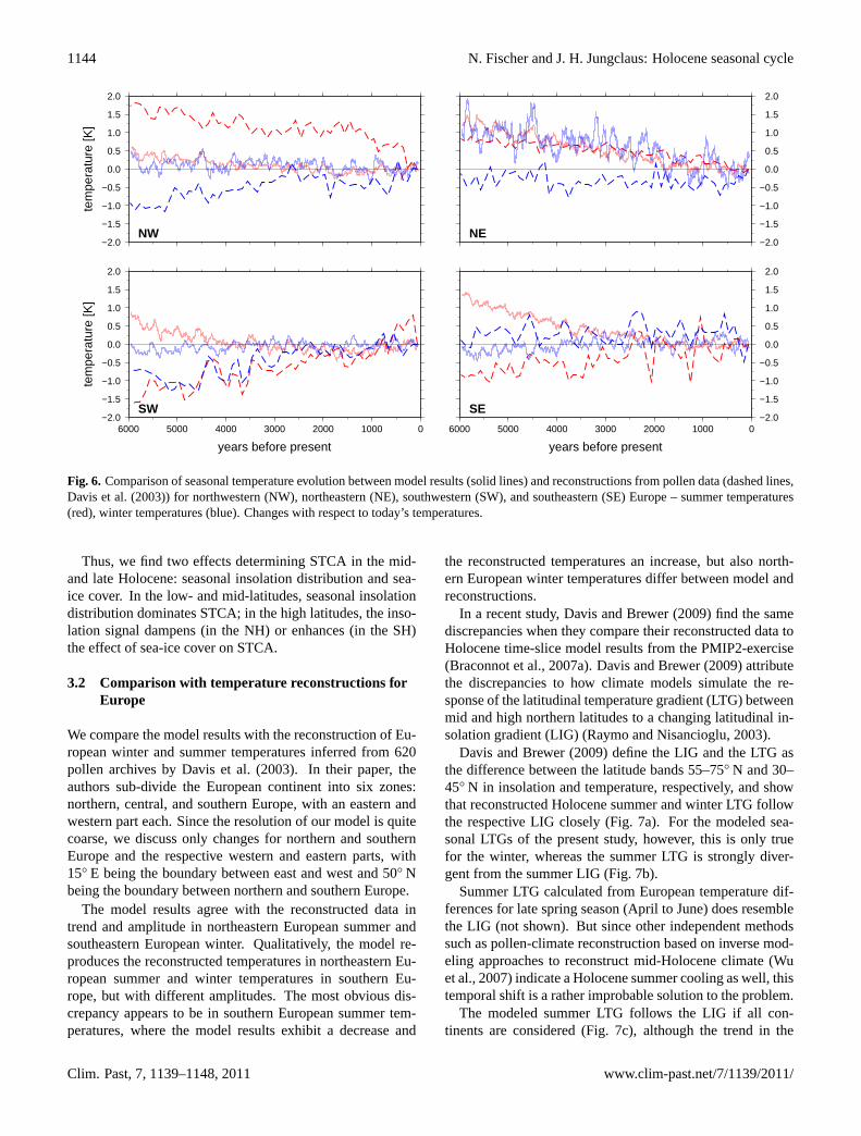
Decreasing summer insolation in the high northern lati-tudes reduces summer sea-ice melt and therefore leads to anincrease in the September sea-ice extend in the Arctic Oceanfrom 70 % to 80 % (Fig.5). In the annual mean, sea-ice coverincreases from 90 to 95 %. With reduced sea-ice cover undermid-Holocene conditions, the ocean acts as a reservoir, gain-ing heat in the summer months and releasing it in the wintermonths, and thus dampening the STCA. Due to the increasein sea-ice cover throughout the simulation, the sea ice acts asan insulator and inhibits the heat reservoir effect. As a con-sequence, the annual mean atmosphere-ocean heat flux overthe Arctic decreases in absolute values by 13 % from−7.4 to−6.6 W m−2 (positive values indicate heat flux directed fromthe atmosphere to the ocean). The seasonal cycle of heat fluxover the Arctic Ocean (Fig.5) decreases by 22 %, with thesummer heat flux decreasing from 70 to 52 W m−2 (24 %)and the winter heat flux decreasing in absolute values from−36 to−28 W m−2 (22 %). For comparison, the differencein incoming radiation at the top of the atmosphere in summer

−1.0 −0.5 0.0 0.5 1.0

K/ka

Fig. 2. Linear trend in seasonal cycle amplitude (difference between warmest and coldest month) over the

simulation period in K/ka - Kelvin per 1,000 years.

−1.0 −0.5 0.0 0.5 1.0

K/ka

Fig. 3. Linear trend in annual mean surface temperature over the simulation period in K/ka - Kelvin per 1,000

years

14

Fig. 3. Linear trend in annual mean surface temperature over thesimulation period in K ka−1 – Kelvin per 1000 yr

is 30 W m−2 (6.6 %) and 12.66 W m−2 (16 %) for the net sur-face shortwave radiation.

The decrease in the amplitude of the seasonal cycle of sea-ice is due to an increase in summer sea-ice cover and thecontinental boundaries of the Arctic Ocean basin that limitwinter sea-ice extent when the whole basin is sea-ice cov-ered. In the Arctic Ocean, especially over the Barents Shelfand along the east coast of Greenland, cooling is enhancedwhere sea ice is expanding. The cooling signal is strongest inautumn and in winter, when – compared to the mid-Holoceneconditions – sea-ice cover acts as an insulator and heat fluxbetween the ocean and the atmosphere is inhibited. Thus, theautumn and winter temperatures sink, despite the fact thatwinter insolation is not changing significantly. So the sea-iceinsulation effect dominates the STCA. This is similar to themechanism proposed to explain the abrupt climate changesin the last 60 000 yr inDenton et al.(2005). Extensive wintersea-ice cover in the Arctic Ocean leads to “continental” cli-mate conditions over the Arctic region and cooler winters inthe late Holocene compared to the mid-Holocene, when re-duced sea-ice cover and thus open ocean in the Arctic regionacts as a heat reservoir and thus leads to warmer winters.

This affects not only the Arctic Ocean, but also influencesthe adjacent continents. The sea-ice insulation effect couldbe amplified by a synergy of the sea-ice albedo effect andthe snow-albedo feedback due to the shift of the northerntree-line in the Holocene. The strength of the synergetic ef-fect of the sea-ice albedo and the snow-albedo feedbacks inthe model setup used here, however, have been shown to besmall (Otto et al., 2009). This might be related to the fact thatthe soil albedo is static in the current model setup and doesnot evolve with vegetation changes. Using a different model,Renssen et al.(2005) showed that the vegetation feedbackis indeed important for summer temperature changes in thehigh northern latitudes. The strength of this effect could po-tentially increase by including a dynamic soil albedo scheme(Vamborg et al., 2011) in the current model.

Clim. Past, 7, 1139–1148, 2011 www.clim-past.net/7/1139/2011/

N. Fischer and J. H. Jungclaus: Holocene seasonal cycle 1143

22 4

4

6

6

6

8

8

8

10

10

12

12

14

14

16

18

years before present

latit

ude[

°N]

DJF

−5000 −4000 −3000 −2000 −1000 0

−60

−30

0

30

60

−2

−2

0

0

2

2

4

4

68

1012

14

years before present

latit

ude[

°N]

MAM

−5000 −4000 −3000 −2000 −1000 0

−60

−30

0

30

60

−25−20−15

−10

−10

−5

−5

0

00

years before present

latit

ude[

°N]

JJA

−5000 −4000 −3000 −2000 −1000 0

−60

−30

0

30

60

−16−14

−12

−10−8

−6

−6

−4

−4

−2

−2

0

02

2

years before present

latit

ude[

°N]

SON

−5000 −4000 −3000 −2000 −1000 0

−60

−30

0

30

60

seasonal insolation diff

Fig. 4. Changes in seasonal insolation from the mid-Holocene to today in W/m2 (winter - DJF, spring - MAM,

Summer - JJA, autumn - SON, seasons are defined after present-day’s calendar). The reference is 6,000 years

before present.

15

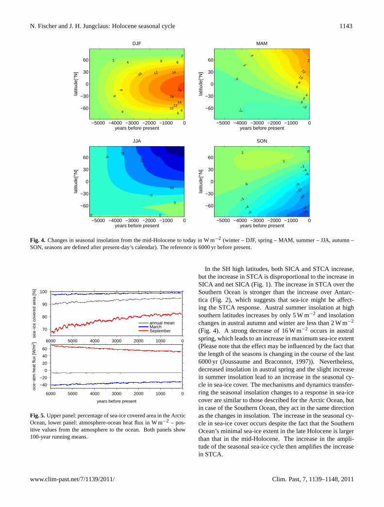
Fig. 4. Changes in seasonal insolation from the mid-Holocene to today in W m−2 (winter – DJF, spring – MAM, summer – JJA, autumn –SON, seasons are defined after present-day’s calendar). The reference is 6000 yr before present.

70

80

90

100

sea−

ice

cove

red

area

[%]

0100020003000400050006000

annual meanMarchSeptember

−40

−20

0

20

40

60

oce−

atm

hea

t flu

x [W

/m2 ]

0100020003000400050006000

years before present

.

Fig. 5. Upper panel: percentage of sea-ice covered area in the Arctic Ocean, lower panel: atmosphere-ocean

heat flux in W/m2 - positive values from the atmosphere to the ocean. Both panels show 100 year running

means.

−2.0

−1.5

−1.0

−0.5

0.0

0.5

1.0

1.5

2.0

tem

pera

ture

[K]

NW−2.0

−1.5

−1.0

−0.5

0.0

0.5

1.0

1.5

2.0

NE

−2.0

−1.5

−1.0

−0.5

0.0

0.5

1.0

1.5

2.0

tem

pera

ture

[K]

0100020003000400050006000

years before present

SW−2.0

−1.5

−1.0

−0.5

0.0

0.5

1.0

1.5

2.0

0100020003000400050006000

years before present

SE

Fig. 6. Comparison of seasonal temperature evolution between model results (solid lines) and reconstructions

from pollen data (dashed lines) for northwestern (NW), northeastern (NE), southwestern (SW), and southeast-

ern (SE) Europe - summer temperatures (red), winter temperatures (blue). Changes with respect to today’s

temperatures.

16

Fig. 5. Upper panel: percentage of sea-ice covered area in the ArcticOcean, lower panel: atmosphere-ocean heat flux in W m−2 – pos-itive values from the atmosphere to the ocean. Both panels show100-year running means.

In the SH high latitudes, both SICA and STCA increase,but the increase in STCA is disproportional to the increase inSICA and net SICA (Fig.1). The increase in STCA over theSouthern Ocean is stronger than the increase over Antarc-tica (Fig. 2), which suggests that sea-ice might be affect-ing the STCA response. Austral summer insolation at highsouthern latitudes increases by only 5 W m−2 and insolationchanges in austral autumn and winter are less than 2 W m−2

(Fig. 4). A strong decrease of 16 W m−2 occurs in australspring, which leads to an increase in maximum sea-ice extent(Please note that the effect may be influenced by the fact thatthe length of the seasons is changing in the course of the last6000 yr (Joussaume and Braconnot, 1997)). Nevertheless,decreased insolation in austral spring and the slight increasein summer insolation lead to an increase in the seasonal cy-cle in sea-ice cover. The mechanisms and dynamics transfer-ring the seasonal insolation changes to a response in sea-icecover are similar to those described for the Arctic Ocean, butin case of the Southern Ocean, they act in the same directionas the changes in insolation. The increase in the seasonal cy-cle in sea-ice cover occurs despite the fact that the SouthernOcean’s minimal sea-ice extent in the late Holocene is largerthan that in the mid-Holocene. The increase in the ampli-tude of the seasonal sea-ice cycle then amplifies the increasein STCA.

www.clim-past.net/7/1139/2011/ Clim. Past, 7, 1139–1148, 2011

1144 N. Fischer and J. H. Jungclaus: Holocene seasonal cycle

70

80

90

100

sea−

ice

cove

red

area

[%]

0100020003000400050006000

annual meanMarchSeptember

−40

−20

0

20

40

60

oce−

atm

hea

t flu

x [W

/m2 ]

0100020003000400050006000

years before present

.

Fig. 5. Upper panel: percentage of sea-ice covered area in the Arctic Ocean, lower panel: atmosphere-ocean

heat flux in W/m2 - positive values from the atmosphere to the ocean. Both panels show 100 year running

means.

−2.0

−1.5

−1.0

−0.5

0.0

0.5

1.0

1.5

2.0te

mpe

ratu

re [K

]

NW−2.0

−1.5

−1.0

−0.5

0.0

0.5

1.0

1.5

2.0

NE

−2.0

−1.5

−1.0

−0.5

0.0

0.5

1.0

1.5

2.0

tem

pera

ture

[K]

0100020003000400050006000

years before present

SW−2.0

−1.5

−1.0

−0.5

0.0

0.5

1.0

1.5

2.0

0100020003000400050006000

years before present

SE

Fig. 6. Comparison of seasonal temperature evolution between model results (solid lines) and reconstructions

from pollen data (dashed lines) for northwestern (NW), northeastern (NE), southwestern (SW), and southeast-

ern (SE) Europe - summer temperatures (red), winter temperatures (blue). Changes with respect to today’s

temperatures.

16

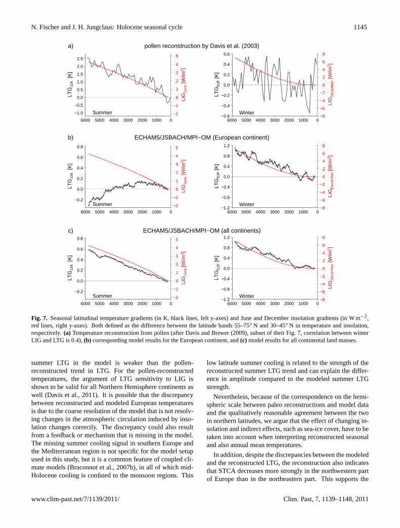
Fig. 6. Comparison of seasonal temperature evolution between model results (solid lines) and reconstructions from pollen data (dashed lines,Davis et al.(2003)) for northwestern (NW), northeastern (NE), southwestern (SW), and southeastern (SE) Europe – summer temperatures(red), winter temperatures (blue). Changes with respect to today’s temperatures.

Thus, we find two effects determining STCA in the mid-and late Holocene: seasonal insolation distribution and sea-ice cover. In the low- and mid-latitudes, seasonal insolationdistribution dominates STCA; in the high latitudes, the inso-lation signal dampens (in the NH) or enhances (in the SH)the effect of sea-ice cover on STCA.

3.2 Comparison with temperature reconstructions forEurope

We compare the model results with the reconstruction of Eu-ropean winter and summer temperatures inferred from 620pollen archives byDavis et al.(2003). In their paper, theauthors sub-divide the European continent into six zones:northern, central, and southern Europe, with an eastern andwestern part each. Since the resolution of our model is quitecoarse, we discuss only changes for northern and southernEurope and the respective western and eastern parts, with15◦ E being the boundary between east and west and 50◦ Nbeing the boundary between northern and southern Europe.

The model results agree with the reconstructed data intrend and amplitude in northeastern European summer andsoutheastern European winter. Qualitatively, the model re-produces the reconstructed temperatures in northeastern Eu-ropean summer and winter temperatures in southern Eu-rope, but with different amplitudes. The most obvious dis-crepancy appears to be in southern European summer tem-peratures, where the model results exhibit a decrease and

the reconstructed temperatures an increase, but also north-ern European winter temperatures differ between model andreconstructions.

In a recent study,Davis and Brewer(2009) find the samediscrepancies when they compare their reconstructed data toHolocene time-slice model results from the PMIP2-exercise(Braconnot et al., 2007a). Davis and Brewer(2009) attributethe discrepancies to how climate models simulate the re-sponse of the latitudinal temperature gradient (LTG) betweenmid and high northern latitudes to a changing latitudinal in-solation gradient (LIG) (Raymo and Nisancioglu, 2003).

Davis and Brewer(2009) define the LIG and the LTG asthe difference between the latitude bands 55–75◦ N and 30–45◦ N in insolation and temperature, respectively, and showthat reconstructed Holocene summer and winter LTG followthe respective LIG closely (Fig.7a). For the modeled sea-sonal LTGs of the present study, however, this is only truefor the winter, whereas the summer LTG is strongly diver-gent from the summer LIG (Fig.7b).

Summer LTG calculated from European temperature dif-ferences for late spring season (April to June) does resemblethe LIG (not shown). But since other independent methodssuch as pollen-climate reconstruction based on inverse mod-eling approaches to reconstruct mid-Holocene climate (Wuet al., 2007) indicate a Holocene summer cooling as well, thistemporal shift is a rather improbable solution to the problem.

The modeled summer LTG follows the LIG if all con-tinents are considered (Fig.7c), although the trend in the

Clim. Past, 7, 1139–1148, 2011 www.clim-past.net/7/1139/2011/

N. Fischer and J. H. Jungclaus: Holocene seasonal cycle 1145

−1.0

−0.5

0.0

0.5

1.0

1.5

2.0

2.5

LTG

JJA [

K]

0100020003000400050006000−2

−1

0

1

2

3

4

5

LIG

June

[W/m

2 ]

Summer−0.6

−0.4

−0.2

0.0

0.2

0.4

0.6

LTG

DJF

[K]

0100020003000400050006000−8

−6

−4

−2

0

2

4

6

8

LIG

Dec

embe

r [W

/m2 ]

Winter

−0.2

0.0

0.2

0.4

0.6

0.8

LTG

JJA [

K]

0100020003000400050006000−2

−1

0

1

2

3

4

5

LIG

June

[W/m

2 ]

Summer−1.2

−0.8

−0.4

0.0

0.4

0.8

1.2

LTG

DJF

[K]

0100020003000400050006000−8

−6

−4

−2

0

2

4

6

8

LIG

Dec

embe

r [W

/m2 ]

Winter

−0.2

0.0

0.2

0.4

0.6

0.8

LTG

JJA [

K]

0100020003000400050006000−2

−1

0

1

2

3

4

5

LIG

June

[W/m

2 ]

Summer−1.2

−0.8

−0.4

0.0

0.4

0.8

1.2

LTG

DJF

[K]

0100020003000400050006000−8

−6

−4

−2

0

2

4

6

8

LIG

Dec

embe

r [W

/m2 ]

Winter

pollen reconstruction by Davis et al. (2003)

ECHAM5/JSBACH/MPI−OM (European continent)

ECHAM5/JSBACH/MPI−OM (all continents)

a)

b)

c)

Fig. 7. Seasonal latitudinal temperature gradients (in K, black lines, left y-axes) and June and December

insolation gradients (in W/m2, red lines, right y-axes). Both defined as the difference between the latitude

bands 55 - 75◦N and 30 - 45◦N in temperature and insolation, respectively.a) temperature reconstruction from

pollen (after Davis and Brewer (2009), subset of their figure7, correlation between winter LIG and LTG is 0.4),

b) corresponding model results for the European continent, and c) model results for all continental land masses.

17

Fig. 7. Seasonal latitudinal temperature gradients (in K, black lines, left y-axes) and June and December insolation gradients (in W m−2,red lines, right y-axes). Both defined as the difference between the latitude bands 55–75◦ N and 30–45◦ N in temperature and insolation,respectively.(a) Temperature reconstruction from pollen (afterDavis and Brewer(2009), subset of their Fig. 7, correlation between winterLIG and LTG is 0.4),(b) corresponding model results for the European continent, and(c) model results for all continental land masses.

summer LTG in the model is weaker than the pollen-reconstructed trend in LTG. For the pollen-reconstructedtemperatures, the argument of LTG sensitivity to LIG isshown to be valid for all Northern Hemisphere continents aswell (Davis et al., 2011). It is possible that the discrepancybetween reconstructed and modeled European temperaturesis due to the coarse resolution of the model that is not resolv-ing changes in the atmospheric circulation induced by inso-lation changes correctly. The discrepancy could also resultfrom a feedback or mechanism that is missing in the model.The missing summer cooling signal in southern Europe andthe Mediterranean region is not specific for the model setupused in this study, but it is a common feature of coupled cli-mate models (Braconnot et al., 2007b), in all of which mid-Holocene cooling is confined to the monsoon regions. This

low latitude summer cooling is related to the strength of thereconstructed summer LTG trend and can explain the differ-ence in amplitude compared to the modeled summer LTGstrength.

Nevertheless, because of the correspondence on the hemi-spheric scale between paleo reconstructions and model dataand the qualitatively reasonable agreement between the twoin northern latitudes, we argue that the effect of changing in-solation and indirect effects, such as sea-ice cover, have to betaken into account when interpreting reconstructed seasonaland also annual mean temperatures.

In addition, despite the discrepancies between the modeledand the reconstructed LTG, the reconstruction also indicatesthat STCA decreases more strongly in the northwestern partof Europe than in the northeastern part. This supports the

www.clim-past.net/7/1139/2011/ Clim. Past, 7, 1139–1148, 2011

1146 N. Fischer and J. H. Jungclaus: Holocene seasonal cycle

−0.5

0.0

0.5

NA

O in

dex

0100020003000400050006000

years before present

Fig. 8. Time-series of North Atlantic Oscillation index calculated from the first EOF of winter mean sea level

pressure over the North Atlantic region (30-year running mean).

18

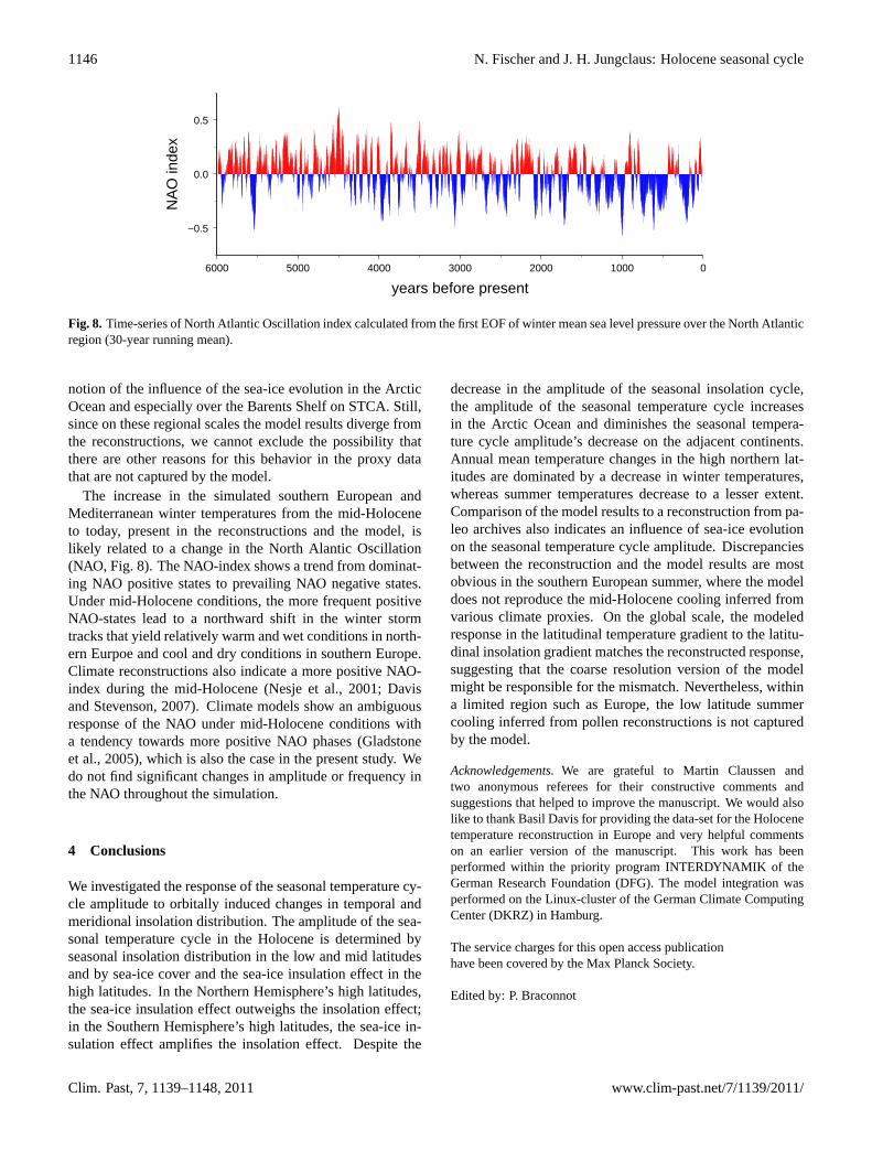
Fig. 8. Time-series of North Atlantic Oscillation index calculated from the first EOF of winter mean sea level pressure over the North Atlanticregion (30-year running mean).

notion of the influence of the sea-ice evolution in the ArcticOcean and especially over the Barents Shelf on STCA. Still,since on these regional scales the model results diverge fromthe reconstructions, we cannot exclude the possibility thatthere are other reasons for this behavior in the proxy datathat are not captured by the model.

The increase in the simulated southern European andMediterranean winter temperatures from the mid-Holoceneto today, present in the reconstructions and the model, islikely related to a change in the North Alantic Oscillation(NAO, Fig.8). The NAO-index shows a trend from dominat-ing NAO positive states to prevailing NAO negative states.Under mid-Holocene conditions, the more frequent positiveNAO-states lead to a northward shift in the winter stormtracks that yield relatively warm and wet conditions in north-ern Eurpoe and cool and dry conditions in southern Europe.Climate reconstructions also indicate a more positive NAO-index during the mid-Holocene (Nesje et al., 2001; Davisand Stevenson, 2007). Climate models show an ambiguousresponse of the NAO under mid-Holocene conditions witha tendency towards more positive NAO phases (Gladstoneet al., 2005), which is also the case in the present study. Wedo not find significant changes in amplitude or frequency inthe NAO throughout the simulation.

4 Conclusions

We investigated the response of the seasonal temperature cy-cle amplitude to orbitally induced changes in temporal andmeridional insolation distribution. The amplitude of the sea-sonal temperature cycle in the Holocene is determined byseasonal insolation distribution in the low and mid latitudesand by sea-ice cover and the sea-ice insulation effect in thehigh latitudes. In the Northern Hemisphere’s high latitudes,the sea-ice insulation effect outweighs the insolation effect;in the Southern Hemisphere’s high latitudes, the sea-ice in-sulation effect amplifies the insolation effect. Despite the

decrease in the amplitude of the seasonal insolation cycle,the amplitude of the seasonal temperature cycle increasesin the Arctic Ocean and diminishes the seasonal tempera-ture cycle amplitude’s decrease on the adjacent continents.Annual mean temperature changes in the high northern lat-itudes are dominated by a decrease in winter temperatures,whereas summer temperatures decrease to a lesser extent.Comparison of the model results to a reconstruction from pa-leo archives also indicates an influence of sea-ice evolutionon the seasonal temperature cycle amplitude. Discrepanciesbetween the reconstruction and the model results are mostobvious in the southern European summer, where the modeldoes not reproduce the mid-Holocene cooling inferred fromvarious climate proxies. On the global scale, the modeledresponse in the latitudinal temperature gradient to the latitu-dinal insolation gradient matches the reconstructed response,suggesting that the coarse resolution version of the modelmight be responsible for the mismatch. Nevertheless, withina limited region such as Europe, the low latitude summercooling inferred from pollen reconstructions is not capturedby the model.

Acknowledgements.We are grateful to Martin Claussen andtwo anonymous referees for their constructive comments andsuggestions that helped to improve the manuscript. We would alsolike to thank Basil Davis for providing the data-set for the Holocenetemperature reconstruction in Europe and very helpful commentson an earlier version of the manuscript. This work has beenperformed within the priority program INTERDYNAMIK of theGerman Research Foundation (DFG). The model integration wasperformed on the Linux-cluster of the German Climate ComputingCenter (DKRZ) in Hamburg.

The service charges for this open access publicationhave been covered by the Max Planck Society.

Edited by: P. Braconnot

Clim. Past, 7, 1139–1148, 2011 www.clim-past.net/7/1139/2011/

N. Fischer and J. H. Jungclaus: Holocene seasonal cycle 1147

References

Berger, A.: Long-Term Variations Of Daily Insolation And Quater-nary Climatic Changes, J. Atmos. Sci., 35, 2362–2367, 1978.

Braconnot, P., Otto-Bliesner, B., Harrison, S., Joussaume, S., Pe-terchmitt, J.-Y., Abe-Ouchi, A., Crucifix, M., Driesschaert, E.,Fichefet, Th., Hewitt, C. D., Kageyama, M., Kitoh, A., Lan, A.,Loutre, M.-F., Marti, O., Merkel, U., Ramstein, G., Valdes, P.,Weber, S. L., Yu, Y., and Zhao, Y.: Results of PMIP2 coupledsimulations of the Mid-Holocene and Last Glacial Maximum -Part 1: experiments and large-scale features, Clim. Past, 3, 261–277, doi:10.5194/cp-3-261-2007, 2007a.

Braconnot, P., Otto-Bliesner, B., Harrison, S., Joussaume, S., Pe-terchmitt, J.-Y., Abe-Ouchi, A., Crucifix, M., Driesschaert, E.,Fichefet, Th., Hewitt, C. D., Kageyama, M., Kitoh, A., Loutre,M.-F., Marti, O., Merkel, U., Ramstein, G., Valdes, P., Weber,L., Yu, Y., and Zhao, Y.: Results of PMIP2 coupled simula-tions of the Mid-Holocene and Last Glacial Maximum - Part2: feedbacks with emphasis on the location of the ITCZ andmid- and high latitudes heat budget, Clim. Past, 3, 279–296,doi:10.5194/cp-3-279-2007, 2007b.

Bretagnon, P. and Francou, G.: Planetary theories in rectangularand spherical variables – VSOP 87 solutions, Astron. Astrophys.,202, 309–315, 1988.

Brovkin, V., Raddatz, T., Reick, C. H., Claussen, M., and Gayler, V.:Global biogeophysical interactions between forest and climate,Geophys. Res. Lett., 36, L07405,doi:10.1029/2009GL037543,2009.

Cheddadi, R., Yu, G., Guiot, J., Harrison, S. P., and Prentice, I. C.:The climate of Europe 6000 years ago, Clim. Dynam., 13, 1–9,doi:10.1007/s003820050148, 1996.

Claussen, M., Kubatzki, C., Brovkin, V., Ganopolski, A., Hoelz-mann, P., and Pachur, H.-J.: Simulation of an abrupt change inSaharan vegetation in the Mid-Holocene, Geophys. Res. Lett.,26, 2037–2040,doi:10.1029/1999GL900494, 1999.

Davis, B. and Brewer, S.: Orbital forcing and role of the latitudi-nal insolation/temperature gradient, Clim. Dynam., 32, 143–165,doi:10.1007/s00382-008-0480-9, 2009.

Davis, B. A. and Stevenson, A. C.: The 8.2 ka event andEarly-Mid Holocene forests, fires and flooding in the CentralEbro Desert, NE Spain, Quaternary Sci. Rev., 26, 1695–1712,doi:10.1016/j.quascirev.2007.04.007, 2007.

Davis, B. A. S., Brewer, S., Stevenson, A. C., Guiot, J., and Con-tributors, D.: The temperature of Europe during the Holocenereconstructed from pollen data, Quaternary Sci. Rev., 22, 1701–1716, 2003.

Denton, G. H., Alley, R. B., Comer, G. C., and Broecker, W. S.:The role of seasonality in abrupt climate change, Quaternary Sci.Rev., 24, 1159–1182, doi:DOI:10.1016/j.quascirev.2004.12.002,2005.

Fischer, N. and Jungclaus, J. H.: Effects of orbital forcing on at-mosphere and ocean heat transports in Holocene and Eemianclimate simulations with a comprehensive Earth system model,Clim. Past, 6, 155–168,doi:10.5194/cp-6-155-2010, 2010.

Gladstone, R. M., Ross, I., Valdes, P. J., Abe-Ouchi, A., Braconnot,P., Brewer, S., Kageyama, M., Kitoh, A., Legrande, A., Marti,O., Ohgaito, R., Otto-Bliesner, B., Peltier, W. R., and Vettoretti,G.: Mid-Holocene NAO: A PMIP2 model intercomparison, Geo-phys. Res. Lett., 32, L16707,doi:10.1029/2005GL023596, 2005.

Hibler, W.: Dynamic thermodynamic sea ice model, J. Pys.

Oceanogr., 9, 815–846, 1979.Joussaume, S. and Braconnot, P.: Sensitivity of paleoclimate simu-

lation results to season definitions, J. Geophys. Res., 102, 1943–1956,doi:10.1029/96JD01989, 1997.

Jungclaus, J. H., Keenlyside, N., Botzet, M., Haak, H., Luo, J. J.,Latif, M., Marotzke, J., Mikolajewicz, U., and Roeckner, E.:Ocean circulation and tropical variability in the coupled modelECHAM5/MPI-OM, J. Climate, 19, 3952–3972, 2006.

Liu, Z., Wang, Y., Gallimore, R., Notaro, M., and Prentice, I. C.: Onthe cause of abrupt vegetation collapse in North Africa during theHolocene: Climate variability vs. vegetation feedback, Geophys.Res. Lett., 33, L22709,doi:10.1029/2006GL028062, 2006.

Lorenz, S. J., Kim, J., Rimbu, N., Schneider, R. R., and Lohmann,G.: Orbitally driven insolation forcing on Holocene climatetrends: Evidence from alkenone data and climate modeling, Pale-oceanography, 21, PA1002,doi:10.1029/2005PA001152, 2006.

Marsland, S. J., Haak, H., Jungclaus, J. H., Latif, M., and Roske,F.: The Max-Planck-Institute global ocean/sea ice model withorthogonal curvilinear coordinates, Ocean Modell., 5, 91–127,2003.

Milankovic, M.: Kanon der Erdbestrahlung und seine Anwendungauf das Eiszeitenproblem, Special Publication, R. Serb. Acad.Belgrade, 132, 633 pp., 1941.

Nesje, A., Matthews, J. A., Dahl, S. O., Berrisford, M. S., andAndersson, C.: Holocene glacier fluctuations of Flatebreen andwinter-precipitation changes in the Jostedalsbreen region, west-ern Norvay, based on glaciolacustrine sediment records, TheHolocene, 11, 267–280, available at:http://hol.sagepub.com/content/11/3/267.abstract, 2001.

Otto, J., Raddatz, T., Claussen, M., Brovkin, V., and Gayler, V.:Separation of atmosphere-ocean-vegetation feedbacks and syner-gies for mid-Holocene climate, Geophys. Res. Lett., 36, L09701,doi:10.1029/2009GL037482, 2009.

Raddatz, T. J., Reick, C. H., Knorr, W., Kattge, J., Roeckner, E.,Schnur, R., Schnitzler, K. G., Wetzel, P., and Jungclaus, J.: Willthe tropical land biosphere dominate the climate-carbon cyclefeedback during the twenty-first century?, Clim. Dynam., 29,565–574, 2007.

Raymo, M. E. and Nisancioglu, K.: The 41 kyr world: Mi-lankovitch’s other unsolved mystery, Paleoceanography, 18,1011,doi:10.1029/2002PA000791, 2003.

Renssen, H., Goosse, H., Fichefet, T., Brovkin, V., Driesschaert,E., and Wolk, F.: Simulating the Holocene climate evolu-tion at northern high latitudes using a coupled atmosphere-sea ice-ocean-vegetation model, Climate Dynamics, 24, 23–43,doi:10.1007/s00382-004-0485-y, 2005.

Renssen, H., Seppa, H., Heiri, O., Roche, D. M., Goosse, H.,and Fichefet, T.: The spatial and temporal complexity ofthe Holocene thermal maximum, Nat. Geosci., 2, 411–414,doi:10.1038/ngeo513, 2009.

Roeckner, E., Bauml, G., Bonaventura, L., Brokopf, R., Esch,M., Giorgetta, M., Hagemann, S., Kirchner, I., Kornblueh,L., Manzini, E., Rhodin, A., Schlese, U., Schulzweida, U.,and Tompkins, A.: The atmospheric general circulation modelECHAM5. Part I: Model description., Tech. Rep. Rep. 349,127 pp., Max Planck Institute for Meteorology, Available fromMPI for Meteorology, Bundesstr. 53, 20146 Hamburg, Germany,2003.

Semtner, A. J.: Model for thermodynamic growth of sea ice in nu-

www.clim-past.net/7/1139/2011/ Clim. Past, 7, 1139–1148, 2011

1148 N. Fischer and J. H. Jungclaus: Holocene seasonal cycle

merical investigations of climate, J. Phys. Oceanogr., 6, 379–389,1976.

Sundqvist, H. S., Zhang, Q., Moberg, A., Holmgren, K., Kornich,H., Nilsson, J., and Brattstrom, G.: Climate change between themid and late Holocene in northern high latitudes - Part 1: Surveyof temperature and precipitation proxy data, Clim. Past, 6, 591–608,doi:10.5194/cp-6-591-2010, 2010.

Tarasov, P. E., Guiot, J., Cheddadi, R., Andreev, A. A., Bezusko,L. G., Blyakharchuk, T. A., Dorofeyuk, N. I., Filimonova, L. V.,Volkova, V. S., and Zernitskaya, V. P.: Climate in northern Eura-sia 6000 years ago reconstructed from pollen data, Earth Planet.Sci. Lett., 171, 635–645,doi:10.1016/S0012-821X(99)00171-5,1999.

Vamborg, F. S. E., Brovkin, V., and Claussen, M.: The effectof a dynamic background albedo scheme on Sahel/Sahara pre-cipitation during the mid-Holocene, Clim. Past, 7, 117–131,doi:10.5194/cp-7-117-2011, 2011.

Wanner, H., Beer, J. Butikofer, J., Crowley, T., Cubasch, U.,Fluckiger, J., Goosse, H., Grosjean, M., Joos, F., Kaplan, J.,Kuttel, M., Muller, S., Prentice, I., Solomina, O., Stocker, T.,Tarasov, P., Wagner, M., and Widmann, M.: Mid- to LateHolocene climate change: an overview, Quaternary Sci. Rev.,27, 1791–1828, 2008.

Wu, H., Guiot, J., Brewer, S., and Guo, Z.: Climatic changesin Eurasia and Africa at the last glacial maximum and mid-Holocene: reconstruction from pollen data using inverse vege-tation modelling, Clim. Dynam., 29, 211–229, 2007.

Clim. Past, 7, 1139–1148, 2011 www.clim-past.net/7/1139/2011/