Evidence for Two Distinct Modes of Large-Scale Ocean Circulation Changesover the Last Century

MIHAI DIMA

Alfred Wegener Institute for Polar and Marine Research, Bremerhaven, Germany, and Faculty of Physics,

University of Bucharest, Bucharest, Romania

GERRIT LOHMANN

Alfred Wegener Institute for Polar and Marine Research, Bremerhaven, Germany

(Manuscript received 30 September 2008, in final form 3 July 2009)

ABSTRACT

Through its nonlinear dynamics and involvement in past abrupt climate shifts the thermohaline circulation

(THC) represents a key element for the understanding of rapid climate changes. The expected THC weak-

ening under global warming is characterized by large uncertainties, and it is therefore of significant impor-

tance to identify ocean circulation changes over the last century. By applying various statistical techniques on

two global sea surface temperature datasets two THC-related modes are separated. The first one involves

relatively slow adjustment of the whole conveyor belt circulation and has an interhemispherically symmetric

pattern. The second mode is associated with the relatively fast adjustment of the North Atlantic overturning

cell and has the seesaw structure. Based on the separation of these two patterns the authors show that the

global conveyor has been weakening since the late 1930s and that the North Atlantic overturning cell suffered

an abrupt shift around 1970. The distinction between the two modes provides also a new frame for inter-

preting past abrupt climate changes.

1. Introduction

The thermohaline circulation (THC) includes cooling-

and brine-release-induced deep convection and sinking

at high latitudes, upwelling elsewhere, and the horizontal

currents that provide the links for the vertical circula-

tions. Here we refer to the global-scale ocean circulation

driven by temperature and salinity anomalies as THC or

conveyor belt circulation (Broecker 1987). The North

Atlantic part of the conveyor is referred to as the NA

THC. Theoretical studies (Stommel 1961) and numerical

experiments (Stocker and Wright 1991) show that it can

suffer abrupt shifts between two different states. The

THC was linked to rapid climate changes in the distant

past, such as for the last glacial period (Dansgaard et al.

1993; Rahmstorf 2002), the last deglaciation (McManus

et al. 2004), the early Holocene (Ellison et al. 2006), the

last millennium (Cronin et al. 2003), and to the modern

global warming (Gregory et al. 2005).

The observed antiphase relation between Greenland

and Antarctic temperatures for the last glacial period

(EPICA Community Members 2006) is explained by

the seesaw concept, which results through an inter-

hemispheric redistribution of heat in response to changes

in the North Atlantic Deep Water (NADW) formation

(Crowley 1992; Broecker 1998; Stocker and Johnsen

2003). However, this concept cannot explain the reported

in-phase variations between the high latitudes of the

hemispheres recorded during the last deglaciation (Steig

et al. 1998).

Numerical integrations show that in response to in-

creased CO2 concentrations the North Atlantic Ocean

becomes warmer and fresher (Gregory et al. 2005) and the

THC weakens (Manabe and Stouffer 2007). Observa-

tional evidence about ocean circulation changes is con-

tradictory. While it was suggested that the THC weakened

over the last decades (Dickson et al. 2002; Bryden et al.

2005), observational (Latif et al. 2006) and numerical

Corresponding author address: Dr. Mihai Dima, University

of Bucharest, Faculty of Physics, Department of Atmospheric

Physics, CP MG-11, Magurele, Str. Atomistilor 405, Bucharest,

Romania.

E-mail: mihai@dmn.ro

1 JANUARY 2010 D I M A A N D L O H M A N N 5

DOI: 10.1175/2009JCLI2867.1

� 2010 American Meteorological Society

studies (Knight et al. 2005) indicate an increased Atlantic

meridional overturning since the 1970s and almost no

trend since the 1920s (Lohmann et al. 2008).

Over the last years a treasure trove of newly digitized

instrumental data about the climate of the last 150 years

has become available. Many of these datasets have a

high quality and high temporal resolution. In particular,

sea surface temperature (SST) represents a key quantity

for ocean–atmosphere interactions and the best avail-

able surface indicator of large-scale oceanic changes.

2. Datasets

We identified the dominant long-term modes of surface

climate variability using global sea surface temperature

fields from two datasets: extended reconstructed SST

version 3 (ERSST.v3) (Smith et al. 2008) and Hadley

Centre Sea Ice and Sea Surface Temperature dataset

(HadISST) (Rayner et al. 2003).

The National Oceanic and Atmospheric Administra-

tion ERSST.v3 dataset is an improved version of the

extended reconstruction 2 (ERSST.v2) developed by

Smith and Reynolds (2004). The major differences be-

tween these two versions are caused by the improved

low-frequency (LF) tuning of ERSST.v3 that reduces

the SST anomaly damping before 1930, using optimized

parameters. Beginning in 1985, ERSST.v3 is also im-

proved by explicitly including bias-adjusted satellite in-

frared data from Advanced Very High Resolution

Radiometer (AVHRR) Pathfinder day and night satel-

lite SST observations. These data improve SST sampling,

especially in the Southern Ocean. They are incorporated

into the improved ERSST.v3 analysis. Information about

sea ice concentrations are used to improve the high lati-

tude SST analysis (Smith and Reynolds 2004). Monthly

SST anomalies are distributed over a 28 3 28 grid and

extend over the 1854–2006 period. Anomalies are relative

to the 1971–2000 period.

HadISST replaces the global sea ice and sea surface

temperature (GISST) dataset and is a unique combi-

nation of monthly globally complete fields of SST and

sea ice concentration on a 18 3 18 grid, extending over

the 1870–2006 period (Rayner et al. 2003). The SST data

are taken from the Met Office Marine Data Bank (MDB),

which from 1982 onward also includes data received

through the Global Telecommunications System. To en-

hance data coverage, monthly median SSTs for 1871–1995

from the Comprehensive Ocean–Atmosphere Data Set

(COADS) were also used where there were no MDB

data. The sea ice data are taken from a variety of sources

including digitized sea ice charts and passive microwave

retrievals. HadISST temperatures are reconstructed

using a two-stage reduced-space optimal interpolation

(RSOI) procedure, followed by superposition of quality-

improved gridded observations onto the reconstructions

to restore local detail. The sea ice fields are made more

homogeneous by compensating satellite microwave-

based sea ice concentrations for the impact of surface

melt effects on retrievals in the Arctic and for algorithm

deficiencies in the Antarctic and by making the histori-

cal in situ concentrations consistent with the satellite

data. SSTs near sea ice are estimated using statistical

relationships between SST and sea ice concentration.

The variability in the Southern Ocean was preserved by

performing a separate RSOI analysis of the extra-

tropical Southern Hemisphere using the in situ and bias-

adjusted AVHRR SSTs for 1982 onward, and then

merging it with the quasi-global fields already created

from the in situ and AVHRR data farther north.

Monthly anomalies are distributed on a 18 3 18 grid and

extend over the 1870–2006 period.

The HadISST analysis follows more closely the

available observations when data are sparse to maximize

the analyzed signal, while the ERSST analyses are more

conservative in sparse-sampling situations in order to

minimize noise. All the analyses were performed for

both fields in order to estimate the robustness of the

results.

3. Methods

The empirical orthogonal functions method (EOF;

Lorentz 1956) is used to identify dominant modes of cli-

mate variability. The EOF technique is effective in sepa-

rating modes with different spatial structures and to

increase the signal-to-noise ratio by identifying the ei-

genmodes of the analyzed field. To identify coupled pat-

terns the canonical correlation analysis method (CCA)

(Preisendorfer 1988) is applied. CCA is a multivariate

method used to identify pairs of modes and their associate

time components in two data fields. It is also a way of

measuring the linear relationship between two multidi-

mensional variables. CCA finds two bases that are optimal

with respect to correlations. For a detailed description of

these methods we refer to von Storch and Zwiers (1999).

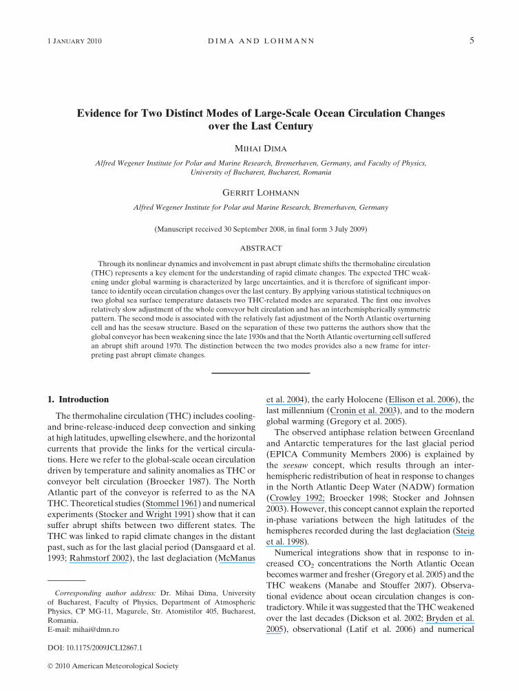
Before the analyses the globally uniform warming

trend was removed by subtracting the annual global

average from each point (Fig. 1). The residual SST fields

are used in all of the analyses presented here.

4. Global modes

Global modes of variability are identified by apply-

ing the EOF method on the annual anomalies of SST.

Aside from the dominant EOF, which is related to the

El Nino–Southern Oscillation (not shown), two modes

6 J O U R N A L O F C L I M A T E VOLUME 23

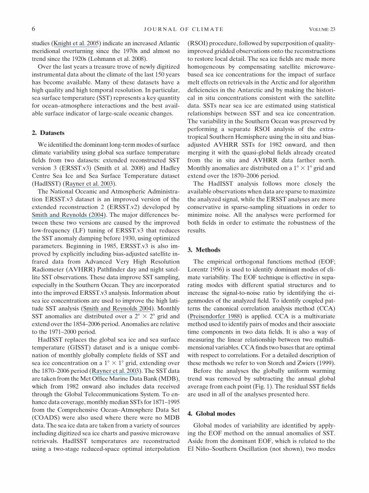
are of specific importance here. They explain 11%

(EOF2) and 7% (EOF3) of variance in the ERSST.v3

dataset and 15% (EOF2) and 5% (EOF4) of variance in

the HadISST fields. If an 11-yr running mean filter is

applied to the data before the analysis, then these two

modes appear to dominate the interdecadal and longer

variations at a global scale.

The first mode [global mode (G)], with very similar

patterns in the two datasets (Figs. 2c,d), has an inter-

hemispherically quasi-symmetric structure and is dom-

inated by prominent localized centers of action. Regions

of positive values are located south of Greenland and

between the Weddell and Ross Seas near Antarctica. An

area of pronounced negative anomalies extends east-

ward from South America to Australia. The time com-

ponent of this mode includes a downward trend since the

late 1930s (Figs. 2a,b). The second mode [Atlantic mode

(A)], is characterized by extended regions of pro-

nounced anomalies in the north and south of the At-

lantic and Pacific basins and by an interhemispheric

asymmetry (Figs. 2e,f). The time evolution of this mode

is dominated by pronounced multidecadal variability

(Figs. 2g,h).

5. Atlantic coupled modes

Because both modes identified through EOF analysis

show large values in the Atlantic Ocean where the THC

induces meridional exchanges of mass and heat, we

performed canonical correlation analyses between the

northern and southern parts of this ocean basin. The

annual fields from the ERSST.v3 and HadISST datasets

are used in two CCAs to identify the most coupled

SST patterns for the regions: 808N–08, 808W–208E and

808S–08, 708W–308E.

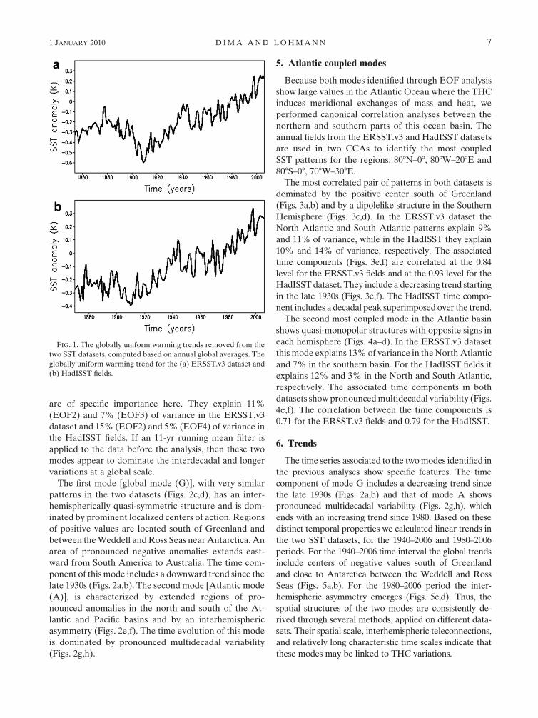
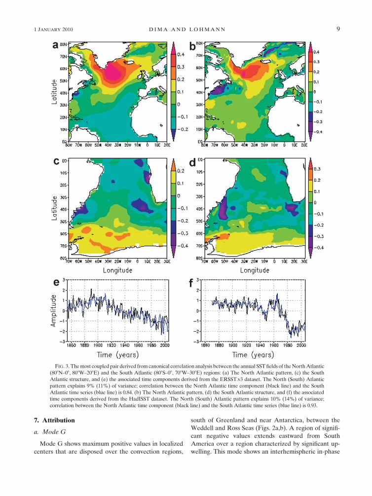
The most correlated pair of patterns in both datasets is

dominated by the positive center south of Greenland

(Figs. 3a,b) and by a dipolelike structure in the Southern

Hemisphere (Figs. 3c,d). In the ERSST.v3 dataset the

North Atlantic and South Atlantic patterns explain 9%

and 11% of variance, while in the HadISST they explain

10% and 14% of variance, respectively. The associated

time components (Figs. 3e,f) are correlated at the 0.84

level for the ERSST.v3 fields and at the 0.93 level for the

HadISST dataset. They include a decreasing trend starting

in the late 1930s (Figs. 3e,f). The HadISST time compo-

nent includes a decadal peak superimposed over the trend.

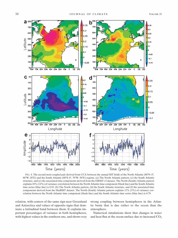
The second most coupled mode in the Atlantic basin

shows quasi-monopolar structures with opposite signs in

each hemisphere (Figs. 4a–d). In the ERSST.v3 dataset

this mode explains 13% of variance in the North Atlantic

and 7% in the southern basin. For the HadISST fields it

explains 12% and 3% in the North and South Atlantic,

respectively. The associated time components in both

datasets show pronounced multidecadal variability (Figs.

4e,f). The correlation between the time components is

0.71 for the ERSST.v3 fields and 0.79 for the HadISST.

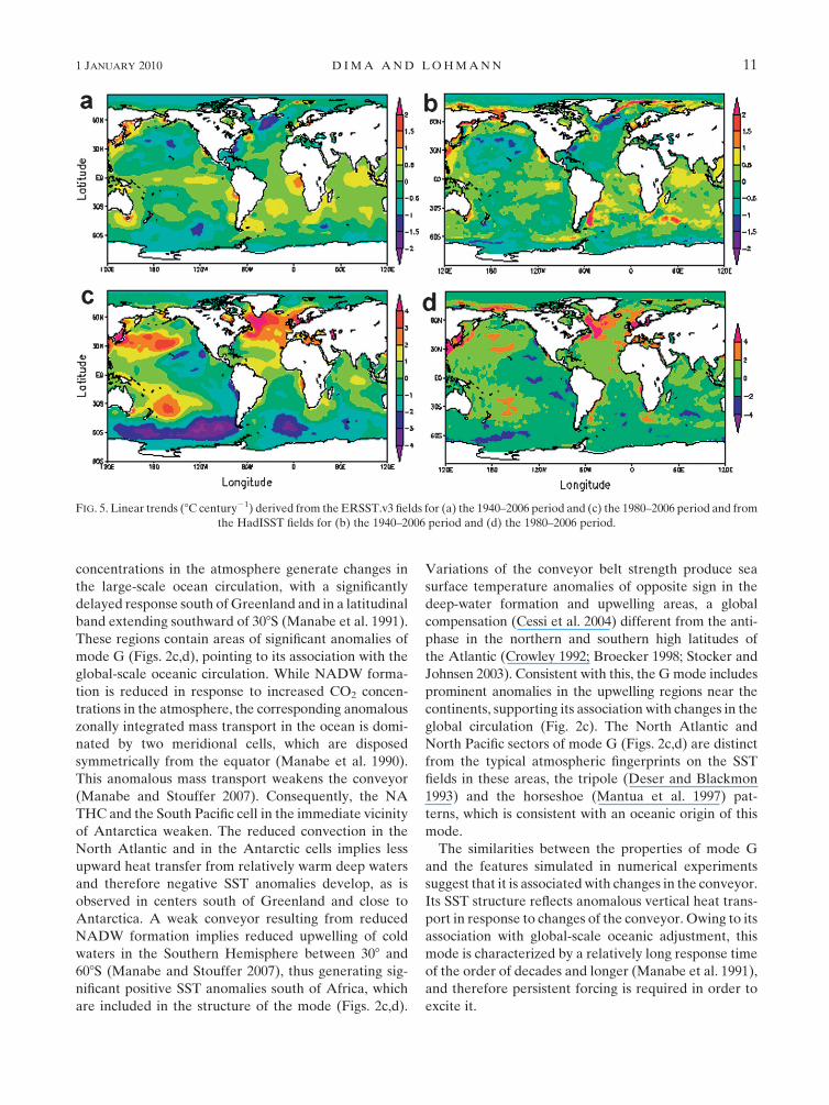
6. Trends

The time series associated to the two modes identified in

the previous analyses show specific features. The time

component of mode G includes a decreasing trend since

the late 1930s (Figs. 2a,b) and that of mode A shows

pronounced multidecadal variability (Figs. 2g,h), which

ends with an increasing trend since 1980. Based on these

distinct temporal properties we calculated linear trends in

the two SST datasets, for the 1940–2006 and 1980–2006

periods. For the 1940–2006 time interval the global trends

include centers of negative values south of Greenland

and close to Antarctica between the Weddell and Ross

Seas (Figs. 5a,b). For the 1980–2006 period the inter-

hemispheric asymmetry emerges (Figs. 5c,d). Thus, the

spatial structures of the two modes are consistently de-

rived through several methods, applied on different data-

sets. Their spatial scale, interhemispheric teleconnections,

and relatively long characteristic time scales indicate that

these modes may be linked to THC variations.

FIG. 1. The globally uniform warming trends removed from the

two SST datasets, computed based on annual global averages. The

globally uniform warming trend for the (a) ERSST.v3 dataset and

(b) HadISST fields.

1 JANUARY 2010 D I M A A N D L O H M A N N 7

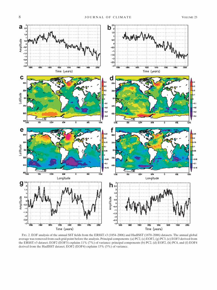
FIG. 2. EOF analysis of the annual SST fields from the ERSST.v3 (1854–2006) and HadISST (1870–2006) datasets. The annual global

average was removed from each grid point before the analysis. Principal components: (a) PC2, (c) EOF2, (g) PC3, (e) EOF3 derived from

the ERSST.v3 dataset; EOF2 (EOF3) explains 11% (7%) of variance: principal components (b) PC2, (d) EOF2, (h) PC4, and (f) EOF4

derived from the HadISST dataset; EOF2 (EOF4) explains 15% (5%) of variance.

8 J O U R N A L O F C L I M A T E VOLUME 23

7. Attribution

a. Mode G

Mode G shows maximum positive values in localized

centers that are disposed over the convection regions,

south of Greenland and near Antarctica, between the

Weddell and Ross Seas (Figs. 2a,b). A region of signifi-

cant negative values extends eastward from South

America over a region characterized by significant up-

welling. This mode shows an interhemispheric in-phase

FIG. 3. The most coupled pair derived from canonical correlation analysis between the annual SST fields of the North Atlantic

(808N–08, 808W–208E) and the South Atlantic (808S–08, 708W–308E) regions: (a) The North Atlantic pattern, (c) the South

Atlantic structure, and (e) the associated time components derived from the ERSST.v3 dataset. The North (South) Atlantic

pattern explains 9% (11%) of variance; correlation between the North Atlantic time component (black line) and the South

Atlantic time series (blue line) is 0.84. (b) The North Atlantic pattern, (d) the South Atlantic structure, and (f) the associated

time components derived from the HadISST dataset. The North (South) Atlantic pattern explains 10% (14%) of variance;

correlation between the North Atlantic time component (black line) and the South Atlantic time series (blue line) is 0.93.

1 JANUARY 2010 D I M A A N D L O H M A N N 9

relation, with centers of the same sign near Greenland

and Antarctica and values of opposite signs that dom-

inate a latitudinal band between them. It explains im-

portant percentages of variance in both hemispheres,

with highest values in the southern one, and shows very

strong coupling between hemispheres in the Atlan-

tic basin that is due rather to the ocean than the

atmosphere.

Numerical simulations show that changes in water

and heat flux at the ocean surface due to increased CO2

FIG. 4. The second most coupled pair derived from CCA between the annual SST fields of the North Atlantic (808N–08,

808W–208E) and the South Atlantic (808S–08, 708W–308E) regions. (a) The North Atlantic pattern, (c) the South Atlantic

structure, and (e) the associated time components derived from the ERSST.v3 dataset. The North (South) Atlantic pattern

explains 10% (14%) of variance; correlation between the North Atlantic time component (black line) and the South Atlantic

time series (blue line) is 0.93. (b) The North Atlantic pattern, (d) the South Atlantic structure, and (f) the associated time

components derived from the HadISST dataset. The North (South) Atlantic pattern explains 12% (3%) of variance; cor-

relation between the North Atlantic time component (black line) and the South Atlantic time series (blue line) is 0.79.

10 J O U R N A L O F C L I M A T E VOLUME 23

concentrations in the atmosphere generate changes in

the large-scale ocean circulation, with a significantly

delayed response south of Greenland and in a latitudinal

band extending southward of 308S (Manabe et al. 1991).

These regions contain areas of significant anomalies of

mode G (Figs. 2c,d), pointing to its association with the

global-scale oceanic circulation. While NADW forma-

tion is reduced in response to increased CO2 concen-

trations in the atmosphere, the corresponding anomalous

zonally integrated mass transport in the ocean is domi-

nated by two meridional cells, which are disposed

symmetrically from the equator (Manabe et al. 1990).

This anomalous mass transport weakens the conveyor

(Manabe and Stouffer 2007). Consequently, the NA

THC and the South Pacific cell in the immediate vicinity

of Antarctica weaken. The reduced convection in the

North Atlantic and in the Antarctic cells implies less

upward heat transfer from relatively warm deep waters

and therefore negative SST anomalies develop, as is

observed in centers south of Greenland and close to

Antarctica. A weak conveyor resulting from reduced

NADW formation implies reduced upwelling of cold

waters in the Southern Hemisphere between 308 and

608S (Manabe and Stouffer 2007), thus generating sig-

nificant positive SST anomalies south of Africa, which

are included in the structure of the mode (Figs. 2c,d).

Variations of the conveyor belt strength produce sea

surface temperature anomalies of opposite sign in the

deep-water formation and upwelling areas, a global

compensation (Cessi et al. 2004) different from the anti-

phase in the northern and southern high latitudes of

the Atlantic (Crowley 1992; Broecker 1998; Stocker and

Johnsen 2003). Consistent with this, the G mode includes

prominent anomalies in the upwelling regions near the

continents, supporting its association with changes in the

global circulation (Fig. 2c). The North Atlantic and

North Pacific sectors of mode G (Figs. 2c,d) are distinct

from the typical atmospheric fingerprints on the SST

fields in these areas, the tripole (Deser and Blackmon

1993) and the horseshoe (Mantua et al. 1997) pat-

terns, which is consistent with an oceanic origin of this

mode.

The similarities between the properties of mode G

and the features simulated in numerical experiments

suggest that it is associated with changes in the conveyor.

Its SST structure reflects anomalous vertical heat trans-

port in response to changes of the conveyor. Owing to its

association with global-scale oceanic adjustment, this

mode is characterized by a relatively long response time

of the order of decades and longer (Manabe et al. 1991),

and therefore persistent forcing is required in order to

excite it.

FIG. 5. Linear trends (8C century21) derived from the ERSST.v3 fields for (a) the 1940–2006 period and (c) the 1980–2006 period and from

the HadISST fields for (b) the 1940–2006 period and (d) the 1980–2006 period.

1 JANUARY 2010 D I M A A N D L O H M A N N 11

b. Mode A

The second mode shows high values over extended

areas at a global scale and a pronounced interhemispheric

asymmetry. It dominates the variability in the North

Atlantic but explains significantly less variance in the

South Atlantic. Mode A shows a strong coupling be-

tween the North and South Atlantic. All of these prop-

erties are consistent with a surface redistribution of heat

in response to changes of the North Atlantic cell

(Crowley 1992; Broecker 1998; Stocker and Johnsen

2003). Weak NADW formation implies reduced north-

ward advection of warm waters by surface currents,

which is compensated by a corresponding southward

transport of heat. However, the effect in the Southern

Hemisphere is highly damped by the extended area

covered by ocean and by the Antarctic Circumpolar

Current, which effectively dissipates the heat (Goosse

and Renssen 2001).

The uniform North Atlantic SST anomalies associated

with mode A (Figs. 2e,f) represent the specific Atlantic

multidecadal oscillation (AMO) (Schlesinger and

Ramankutty 1994) fingerprint (Latif et al. 2004), a mode

which has been linked to NA THC variations (Knight

et al. 2005). The significant larger anomalies recorded in

the North Atlantic as compared to the South Atlantic

and the corresponding multidecadal time scale (Figs.

2g,h) also represent specific AMO features. The fact

that the AMO has a period of about 70 years implies that

the associated forcing must change sign at least twice

during such a time interval (Dima and Lohmann 2007).

Consequently, the response time of this mode can be on

the order of years to decades. Thus, the A mode de-

scribes an interhemispherically asymmetric surface re-

distribution of heat by surface currents as a response to

changes in the NA THC. Due to its relatively small re-

sponse time, it could be excited by pulselike forcing,

characterized by interannual to decadal time scale.

The distinction between these two modes is supported

also by paleodata. The antiphase relation between SST

anomalies, in the North Atlantic and the coastal areas in

the North Pacific sector, of mode G (Fig. 2d) was asso-

ciated with the dominant mode of the Northern Hemi-

sphere SST variability over the Holocene (Kim et al.

2004) and with THC changes over the last glacial period

(Kiefer et al. 2001). Furthermore, it was presented as

evidence of anoxia events over the past 60 000 years,

linked to less upwelling and warmer conditions in the

Santa Barbara Basin (Behl and Kennett 1996) that

correspond to cold periods recorded in the Green-

land ice cap, in agreement with the structure of the G

mode (Fig. 2d). Consistent with the interhemispherically

symmetric SST structure of this mode, the Greenland

Ice Sheet Project 2 (GISP2) and stable isotope records

from Taylor Dome, the closest Antarctic site to the

prominent Antarctic center of positive anomalies (Figs.

2c,d), show in-phase variations during the last degla-

ciation (Steig et al. 1998). Similarly, in agreement with the

interhemispherically asymmetric SST structure of mode

A and with its associated redistribution of heat in the

Atlantic basin, a glacial climate record from an ice core

from the southern edge of the basin (Dronning Maud

Land, Antarctica) shows a one-to-one coupling between

all Antarctic cold events and Greenland warm events by

the bipolar seesaw (EPICA Community Members 2006).

For persistent long-term forcing the whole conveyor

has time to adjust and therefore mode G would domi-

nate. Therefore the interhemispherically symmetric

THC mode could mediate the simultaneous transitions

between glacial and interglacial states in Greenland and

Antarctica at orbital time scales.

8. Implications

Given that a forcing for THC is strong enough, its

temporal properties can determine which mode is ex-

cited. For a pulselike forcing the A mode is excited be-

cause it has a fast response time. For a persistent forcing

the response can be decomposed into two phases. In the

first stage the A mode is excited through the rapid ad-

justment of the NA THC, while in a second phase the

adjustment extends to the whole conveyor and the G

mode replaces the A mode. Such a sequence of two

phases with fast and slow responses to North Atlantic

freshwater forcing was simulated with coupled ocean–

atmosphere general circulation models (Stouffer et al.

2006). These considerations imply that the A mode is

more representative for rapid climate changes, while the

G mode is mainly associated with long-term forcing.

However, both modes can be simultaneously excited by

different forcing.

a. THC trend

A persistent and relatively strong forcing for the

oceanic circulation is represented by the global warming

trend, supposed to be of anthropogenic origin. In re-

sponse to increasing atmospheric CO2 concentration

general circulation models show a gradual THC weak-

ening (Gregory et al. 2005) and surface temperature

structures, which include the Greenland and Antarctic

centers, resembling the G mode (Stouffer et al. 1989;

Haywood et al. 1997; Flato and Boer 2001). A similar

G-like pattern was shown as a response to idealized

long-term freshwater forcing in the North Atlantic

(Manabe and Stouffer 1997; Lohmann 2003) and as

a result of a THC collapse (Tziperman 1997). One of the

12 J O U R N A L O F C L I M A T E VOLUME 23

features of the G mode is its downward trend starting in

the late 1930s. Given its link to global-scale oceanic

adjustment, this implies that the conveyor has been

slowing down over the last seven decades, consistent with

the moderate weakening of the Atlantic overturning

circulation over the last several decades (Hansen et al.

2001; Dickson et al. 2002; Curry et al. 2003; Bryden et al.

2005; Curry and Mauritzen 2005). If one assumes that the

SSTs south of Greenland are of similar magnitudes in

both G and A modes, based on numerical experiments

(Knight et al. 2005), one can estimate a moderate re-

duction of ;15% of the Atlantic overturning as part of

the mode G from the late 1930s to 2006.

b. THC shift

The relatively small response time of mode A implies

that it provides a good representation of rapid THC

changes with interannual and decadal time scales, con-

sistent with previous studies showing that abrupt climate

events associated with fast THC variations are reflected

as an interhemispheric dipole in the surface temperature

field (Goosse et al. 2002; Renssen et al. 2002; LeGrande

et al. 2006). This suggests that an interhemispheric SST

index can be used as a proxy for rapid THC changes. We

show two hemispheric time series, based on the two

datasets, as differences between SST averages over the

Northern and Southern Hemispheres (Figs. 6a,b). The G

mode has a small projection on this index because it

includes bands of alternating signs in each hemisphere

(Figs. 2c,d).

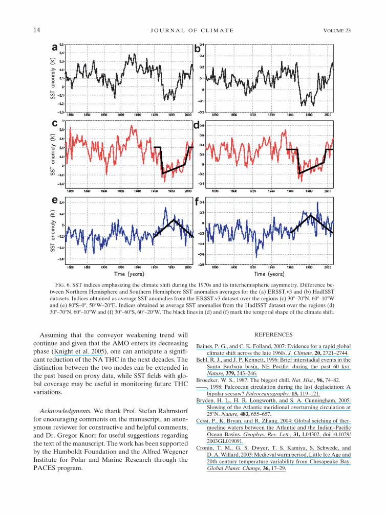
Both time series show interannual variations super-

imposed on pronounced multidecadal variability, cor-

responding to the Atlantic multidecadal oscillation

(Figs. 6a,b). A unique feature in both time series is the

very abrupt change observed around 1970. It represents

a rapid transition of large amplitude, extending over

just several years, to a state corresponding to the lower

interhemispheric gradient in the last 153 years. To in-

vestigate more local representations of the rapid tran-

sition emphasized in the interhemispheric index, four

time series were constructed as SST averages over spe-

cific regions in the Northern and Southern Hemisphere

where the A mode shows large amplitudes.

For the North Atlantic indices the shift is observed

as a fast transition to a state of reduced SST anomalies

(Figs. 6c,d). This state persists 1–2 decades and is then

followed by a gradual recovery to the state of positive SST

anomalies. This resumption to conditions before the

1970s can be caused by the negative feedbacks associated

with the AMO (Dima and Lohmann 2007). The transition

to a new state is also observed in the Southern Hemi-

sphere indices but with a reverse sign, consistent with the

interhemispheric asymmetry of mode A (Figs. 6e,f).

The shapes of the transitions observed in the SST

indices (Fig. 6) are different for the Northern and

Southern Hemisphere. In the North Atlantic an abrupt

decrease is followed by a small-slope metastable state

extending over 1–2 decades and then by a rapid tran-

sition to the preshift conditions. This temporally

asymmetric pattern of change resembles the Atlantic

meridional overturning response to freshwater forcing

(Stouffer et al. 2006). In the South Atlantic the tem-

poral pattern of the shift is more symmetric and in-

cludes more gradual warmings and coolings (Figs. 6e,f).

The interhemispheric structure of this temporal pattern

(with reverse sign) represents a characteristic feature

of the Dansgaard–Oeschger (DO) events (EPICA Com-

munity Members 2006), which were linked to THC var-

iations.

Given the association between the A mode and the

North Atlantic meridional cell (Knight et al. 2005), this

abrupt change can be interpreted as a NA THC shift

between two distinct states, consistent with previous

suggestion (Baines and Folland 2007). Considering the

pronounced Great Salinity Anomaly (GSA) observed in

the late 1960s (Dickson et al. 1988), we speculate that

the THC shift was generated by the GSA.

The distinct properties of modes G and A provide

a base to reconcile previous views about the THC evo-

lution, suggesting an increasing trend since the 1970s

(Latif et al. 2006) versus a potential decreasing trend

since the 1950s (Bryden et al. 2005). While the increasing

trend since 1970s is due to a NA THC intensification,

reflected as an AMO transition from a negative to

a positive phase (Figs. 6a–d), the decreasing trend over

the last seven decades is associated to the weakening of

the conveyor, possibly in response to increased CO2

concentrations in the atmosphere. The THC evolution

results from the combination of G and A modes, which

are associated to different physical processes.

9. Conclusions

The separation of the two ocean modes with different

spatial and temporal properties, resulting from vertical

transfer of heat and from horizontal heat advection by

surface currents, respectively, allows for the identifica-

tion of a THC weakening trend over the last seven de-

cades and a NA THC shift around 1970. During the

modern period the THC variations seem to result from

a combination of these two modes. The fact that,

through a combination of the properties of G and A

modes, one can explain features of modern and paleo-

climate changes implies that THC variations of these

types are operating during both the past and the modern

period (Yu et al. 1996).

1 JANUARY 2010 D I M A A N D L O H M A N N 13

Assuming that the conveyor weakening trend will

continue and given that the AMO enters its decreasing

phase (Knight et al. 2005), one can anticipate a signifi-

cant reduction of the NA THC in the next decades. The

distinction between the two modes can be extended in

the past based on proxy data, while SST fields with glo-

bal coverage may be useful in monitoring future THC

variations.

Acknowledgments. We thank Prof. Stefan Rahmstorf

for encouraging comments on the manuscript, an anon-

ymous reviewer for constructive and helpful comments,

and Dr. Gregor Knorr for useful suggestions regarding

the text of the manuscript. The work has been supported

by the Humboldt Foundation and the Alfred Wegener

Institute for Polar and Marine Research through the

PACES program.

REFERENCES

Baines, P. G., and C. K. Folland, 2007: Evidence for a rapid global

climate shift across the late 1960s. J. Climate, 20, 2721–2744.

Behl, R. J., and J. P. Kennett, 1996: Brief interstadial events in the

Santa Barbara basin, NE Pacific, during the past 60 kyr.

Nature, 379, 243–246.

Broecker, W. S., 1987: The biggest chill. Nat. Hist., 96, 74–82.

——, 1998: Paleocean circulation during the last deglaciation: A

bipolar seesaw? Paleoceanography, 13, 119–121.

Bryden, H. L., H. R. Longworth, and S. A. Cunningham, 2005:

Slowing of the Atlantic meridional overturning circulation at

258N. Nature, 483, 655–657.

Cessi, P., K. Bryan, and R. Zhang, 2004: Global seiching of ther-

mocline waters between the Atlantic and the Indian–Pacific

Ocean Basins. Geophys. Res. Lett., 31, L04302, doi:10.1029/

2003GL019091.

Cronin, T. M., G. S. Dwyer, T. S. Kamiya, S. Schwede, and

D. A. Willard, 2003: Medieval warm period, Little Ice Age and

20th century temperature variability from Chesapeake Bay.

Global Planet. Change, 36, 17–29.

FIG. 6. SST indices emphasizing the climate shift during the 1970s and its interhemispheric asymmetry. Difference be-

tween Northern Hemisphere and Southern Hemisphere SST anomalies averages for the (a) ERSST.v3 and (b) HadISST

datasets. Indices obtained as average SST anomalies from the ERSST.v3 dataset over the regions (c) 308–708N, 608–108W

and (e) 808S–08, 508W–208E. Indices obtained as average SST anomalies from the HadISST dataset over the regions (d)

308–708N, 608–108W and (f) 308–608S, 608–208W. The black lines in (d) and (f) mark the temporal shape of the climate shift.

14 J O U R N A L O F C L I M A T E VOLUME 23

Crowley, T. J., 1992: North Atlantic Deep Water cools the South-

ern Hemisphere. Paleoceanography, 7, 489–497.

Curry, R., and C. Mauritzen, 2005: Dilution of the northern North

Atlantic Ocean in recent decades. Science, 308, 1772–1774.

——, B. Dickson, and I. Yashayaev, 2003: A change in the fresh-

water balance of the Atlantic Ocean over the past four de-

cades. Nature, 426, 826–829.

Dansgaard, W., and Coauthors, 1993: Evidence for general in-

stability of past climate from a 250-kyr ice-core record. Nature,

364, 218–220.

Deser, C., and M. L. Blackmon, 1993: Surface climate variations

over the North Atlantic Ocean during winter. J. Climate, 6,

1743–1753.

Dickson, R. R., J. Meincke, S. A. Malmberg, and A. J. Lee, 1988:

The ‘‘great salinity anomaly’’ in the northern Atlantic 1968–

1982. Prog. Oceanogr., 20, 103–151.

——, Y. Yashayaev, J. Meincke, B. Turrell, S. Dye, and J. Holfort,

2002: Rapid freshening of the deep North Atlantic Ocean over

the past four decades. Nature, 416, 832–837.

Dima, M., and G. Lohmann, 2007: A hemispheric mechanism for the

Atlantic multidecadal oscillation. J. Climate, 20, 2706–2719.

Ellison, C. R., M. R. Chapman, and I. R. Hall, 2006: Surface–deep

ocean interactions during the cold climate event 8200 years

ago. Science, 312, 1929–1932.

EPICA Community Members, 2006: One-to-one coupling of gla-

cial climate variability in Greenland and Antarctica. Nature,

444, 195–198.

Flato, G. M., and G. J. Boer, 2001: Warming asymmetry in climate

change simulations. Geophys. Res. Lett., 28, 195–198.

Goosse, H., and H. A. Renssen, 2001: Two-phase response of the

Southern Ocean to an increase in greenhouse gas concentra-

tions. Geophys. Res. Lett., 28, 3469–3472.

——, H. Renssen, F. M. Selten, R. J. Haarsma, and J. D. Opsteegh,

2002: Potential causes of abrupt climate events: A numerical

study with a three-dimensional climate model. Geophys. Res.

Lett., 29, 1860, doi:10.1029/2002GL014993.

Gregory, J. M., and Coauthors, 2005: A model intercomparison of

changes in the Atlantic thermohaline circulation in response

to increasing atmospheric CO2 concentration. Geophys. Res.

Lett., 32, L12703, doi:10.1029/2005GL023209.

Hansen, B., W. R. Turrell, and S. Osterhus, 2001: Decreasing

overflow from the Nordic seas into the Atlantic Ocean through

the Faroe Bank channel since 1950. Nature, 411, 927–930.

Haywood, J. M., R. J. Stouffer, R. T. Wetherald, S. Manabe, and

V. Ramaswamy, 1997: Transient response of a coupled model

to estimated changes in greenhouse gas and sulfate concen-

trations. Geophys. Res. Lett., 24, 1335–1338.

Kiefer, T., M. Sarnthein, H. Erlenkeuser, P. M. Grootes, and

A. P. Roberts, 2001: North Pacific response to millennial-scale

changes in ocean circulation over the last 60 kyr. Paleo-

ceanography, 16, 179–189.

Kim, J.-H., N. Rimbu, S. J. Lorentz, G. Lohmann, S.-I. Nam,

S. Schouten, C. Ruhlemann, and R. R. Schneider, 2004: Pacific

and North Atlantic sea-surface temperature variability during

Holocene. Quat. Sci. Rev., 23, 2141–2154.

Knight, R. A., R. J. Allan, C. K. Folland, M. Vellinga, and

M. E. A. Mann, 2005: A signature of persistent natural ther-

mohaline circulation cycles in observed climate. Geophys. Res.

Lett., 32, L20708, doi:10.1029/2005GL024233.

Latif, M., and Coauthors, 2004: Reconstructing, monitoring, and

predicting multidecadal-scale changes in the North Atlantic

thermohaline circulation with sea surface temperature.

J. Climate, 17, 1605–1614.

——, C. Boning, J. Willebrand, A. Biastoch, J. Dengg, N. Keenlyside,

U. Schweckendiek, and G. Madec, 2006: Is the thermohaline

circulation changing? J. Climate, 19, 4631–4637.

LeGrande, A. N., G. A. Schmidt, D. T. Shindell, C. V. Field,

R. L. Miller, D. M. Koch, G. Faluvegi, and G. Hoffmann, 2006:

Consistent simulations of multiple proxy responses to an

abrupt climate change event. Proc. Natl. Acad. Sci. USA, 103,

837–842.

Lohmann, G., 2003: Atmospheric and oceanic freshwater transport

during weak Atlantic overturning circulation. Tellus, 55A,

438–449.

——, H. Haak, and J. H. Jungclaus, 2008: Estimating trends of

Atlantic meridional overturning circulation from long-term

hydrografic data and model simulations. Ocean Dyn., 58,

127–138.

Lorentz, E. N., 1956: Empirical orthogonal functions and statistical

weather prediction. Statistical Forecasting Project Scientific

Rep. 1, Defense Doc. Center 110268, Massachusetts Institute

of Technology, 49 pp.

Manabe, S., and R. J. Stouffer, 1997: Coupled ocean–atmosphere

model response to freshwater input: Comparison to Younger

Dryas event. Paleoceanography, 12, 321–336.

——, and ——, 2007: Role of ocean in global warming. J. Meteor.

Soc. Japan, 85, 385–403.

——, K. Bryan, and M. J. Spelman, 1990: Transient response of

a global ocean–atmosphere model to a doubling of atmo-

spheric carbon dioxide. J. Phys. Oceanogr., 20, 722–749.

——, R. J. Stouffer, M. J. Spelman, and K. Bryan, 1991: Transient

responses of a coupled ocean–atmosphere model to gradual

changes of atmospheric CO2. Part I: Annual mean response.

J. Climate, 4, 785–818.

Mantua, N. J., S. R. Hare, Y. Zhang, J. M. Wallace, and

R. C. Francis, 1997: A Pacific interdecadal climate oscillation

with impacts on salmon production. Bull. Amer. Meteor. Soc.,

78, 1069–1079.

McManus, J. F., R. Francois, J.-M. Gherardi, L. D. Kelgwin, and

S. Brown-Leger, 2004: Collapse and rapid resumption of At-

lantic meridional circulation linked to deglacial climate

changes. Nature, 428, 834–837.

Preisendorfer, R. H., 1988: Principal Component Analysis in Me-

teorology and Oceanography. Elsevier, 425 pp.

Rahmstorf, S., 2002: Ocean circulation and climate during the past

120,000 years. Nature, 419, 207–214.

Rayner, N. A., D. E. Parker, E. B. Horton, C. K. Folland,

L. V. Alexander, D. P. Rowell, E. C. Kent, and A. Kaplan, 2003:

Global analyses of sea surface temperature, sea ice, and night

marine air temperature since the late nineteenth century.

J. Geophys. Res., 108, 4407, doi:10.1029/2002JD002670.

Renssen, H., H. Goosse, and T. Fichefet, 2002: Modeling the effect

of freshwater pulses on the early Holocene climate: The in-

fluence of high-frequency climate variability. Paleoceanog-

raphy, 17, 1020, doi:10.1029/2001PA000649.

Schlesinger, M. E., and N. Ramankutty, 1994: An oscillation in the

global climate system of period 65–70 years. Nature, 367,

723–726.

Smith, T. M., and R. W. Reynolds, 2004: Improved extended

reconstruction of SST (1854–1997). J. Climate, 17, 2466–

2477.

——, ——, T. C. Peterson, and J. Lawrimore, 2008: Improvements

to NOAA’s historical merged land–ocean surface tempera-

ture analysis (1880–2006). J. Climate, 21, 2283–2296.

Steig, E. J., and Coauthors, 1998: Synchronous climate changes in

Antarctica and the North Atlantic. Science, 282, 92–95.

1 JANUARY 2010 D I M A A N D L O H M A N N 15

Stocker, T. F., and D. C. Wright, 1991: Rapid transitions of the

ocean’s deep circulation induced by changes in surface water

fluxes. Nature, 27, 729–732.

——, and S. J. Johnsen, 2003: A minimum thermodynamic model for

the bipolar seesaw. Paleoceanography, 18, 1087, doi:10.1029/

2003PA000920.

Stommel, H., 1961: Thermohaline convection with two stable re-

gimes of flow. Tellus, 13, 224–230.

Stouffer, R. J., S. Manabe, and K. Bryan, 1989: Interhemispheric

asymmetry in climate response to a gradual increase of at-

mospheric CO2. Nature, 342, 660–662.

——, and Coauthors, 2006: Investigating the causes of the response

of the thermohaline circulation to past and future climate

changes. J. Climate, 19, 1365–1387.

Tziperman, E., 1997: Inherently unstable climate behaviour

due to weak thermohaline ocean circulation. Nature, 386,

592–595.

von Storch, H. V., and F. W. Zwiers, 1999: Statistical Analysis in

Climate Research. Cambridge University Press, 484 pp.

Yu, E.-F., R. Francois, and M. P. Bacon, 1996: Similar rates of

modern and last-glacial ocean thermohaline circulation in-

ferred from radiochemical data. Nature, 379, 689–694.

16 J O U R N A L O F C L I M A T E VOLUME 23