Evaluation, Selection, and Application of Model-Based Diagnosis Tools and Approaches
26
American Institute of Aeronautics and Astronautics 1 Evaluation, Selection, and Application of Model-Based Diagnosis Tools and Approaches Scott Poll*, Ann Patterson-Hine†, Joe Camisa‡, David Nishikawa§, Lilly Spirkovska§ NASA Ames Research Center, Moffett Field, CA 94035 David Garcia§, David Hall§, Christian Neukom§, Adam Sweet§, Serge Yentus§ QSS Group, Inc., a subsidiary of Perot Systems Government Services, Moffett Field, CA 94035 Charles Lee§, John Ossenfort§ SAIC, Moffett Field, CA 94035 Ole J. Mengshoel§ RIACS, Moffett Field, CA 94035 Indranil Roychoudhury ** , Matthew Daigle ** , Gautam Biswas †† , Xenofon Koutsoukos †† Vanderbilt University, Nashville, TN 37235 and Robyn Lutz ‡‡ Jet Propulsion Lab/Caltech and Iowa State University, Ames, Iowa, 50011 Model-based approaches have proven fruitful in the design and implementation of intelligent systems that provide automated diagnostic functions. A wide variety of models are used in these approaches to represent the particular domain knowledge, including analytic state-based models, input-output transfer function models, fault propagation models, and qualitative and quantitative physics-based models. Diagnostic applications are built around three main steps: observation, comparison, and diagnosis. If the modeling begins in the early stages of system development, engineering models such as fault propagation models can be used for testability analysis to aid definition and evaluation of instrumentation suites for observation of system behavior. Analytical models can be used in the design of monitoring algorithms that process observations to provide information for the second step in the process, comparison of expected behavior of the system to actual measured behavior. In the final diagnostic step, reasoning about the results of the comparison can be performed in a variety of ways, such as dependency matrices, graph propagation, constraint propagation, and state estimation. Realistic empirical evaluation and comparison of these approaches is often hampered by a lack of standard data sets and suitable testbeds. In this paper we describe the Advanced Diagnostics and Prognostics Testbed (ADAPT) at NASA Ames Research Center. The purpose of the testbed is to measure, evaluate, and mature diagnostic and prognostic health management technologies. This paper describes the testbed’s hardware, software architecture, and concept of operations. A simulation testbed that * ADAPT Project Manager, Discovery and Systems Health, MS 269-1, Senior Member † Discovery and Systems Health, MS 269-4, Senior Member ‡ Electronic Systems and Controls Branch, MS 213-2 § Discovery and Systems Health, MS 269-4 ** Department of Electrical Engineering and Computer Science, Institute for Software Integrated Systems †† Professor, Dept. of Electrical Engineering and Computer Science, Institute for Software Integrated Systems ‡‡ Professor, Department of Computer Science
Transcript of Evaluation, Selection, and Application of Model-Based Diagnosis Tools and Approaches

American Institute of Aeronautics and Astronautics
1
Evaluation, Selection, and Application of Model-Based
Diagnosis Tools and Approaches
Scott Poll*, Ann Patterson-Hine†, Joe Camisa‡, David Nishikawa§, Lilly Spirkovska§
NASA Ames Research Center, Moffett Field, CA 94035
David Garcia§, David Hall§, Christian Neukom§, Adam Sweet§, Serge Yentus§
QSS Group, Inc., a subsidiary of Perot Systems Government Services, Moffett Field, CA 94035
Charles Lee§, John Ossenfort§
SAIC, Moffett Field, CA 94035
Ole J. Mengshoel§
RIACS, Moffett Field, CA 94035
Indranil Roychoudhury**, Matthew Daigle
**, Gautam Biswas
††, Xenofon Koutsoukos
††
Vanderbilt University, Nashville, TN 37235
and
Robyn Lutz‡‡
Jet Propulsion Lab/Caltech and Iowa State University, Ames, Iowa, 50011
Model-based approaches have proven fruitful in the design and implementation of
intelligent systems that provide automated diagnostic functions. A wide variety of models are
used in these approaches to represent the particular domain knowledge, including analytic
state-based models, input-output transfer function models, fault propagation models, and
qualitative and quantitative physics-based models. Diagnostic applications are built around
three main steps: observation, comparison, and diagnosis. If the modeling begins in the early
stages of system development, engineering models such as fault propagation models can be
used for testability analysis to aid definition and evaluation of instrumentation suites for
observation of system behavior. Analytical models can be used in the design of monitoring
algorithms that process observations to provide information for the second step in the
process, comparison of expected behavior of the system to actual measured behavior. In the
final diagnostic step, reasoning about the results of the comparison can be performed in a
variety of ways, such as dependency matrices, graph propagation, constraint propagation,
and state estimation. Realistic empirical evaluation and comparison of these approaches is
often hampered by a lack of standard data sets and suitable testbeds. In this paper we
describe the Advanced Diagnostics and Prognostics Testbed (ADAPT) at NASA Ames
Research Center. The purpose of the testbed is to measure, evaluate, and mature diagnostic
and prognostic health management technologies. This paper describes the testbed’s
hardware, software architecture, and concept of operations. A simulation testbed that
* ADAPT Project Manager, Discovery and Systems Health, MS 269-1, Senior Member
† Discovery and Systems Health, MS 269-4, Senior Member
‡ Electronic Systems and Controls Branch, MS 213-2
§ Discovery and Systems Health, MS 269-4
** Department of Electrical Engineering and Computer Science, Institute for Software Integrated Systems
†† Professor, Dept. of Electrical Engineering and Computer Science, Institute for Software Integrated Systems
‡‡ Professor, Department of Computer Science

American Institute of Aeronautics and Astronautics
2
accompanies ADAPT, and some of the diagnostic and decision support approaches being
investigated are also discussed.
I. Introduction
Automated methods for diagnosing problems with system behavior are commonplace in automobiles, copiers,
and many other consumer products. Applying advanced diagnostic techniques to aerospace systems, especially
aerospace vehicles with human crews, is much more challenging. The low probability of component and subsystem
failure, the cost of verification and validation, the difficulty of selecting the most appropriate diagnostic technology
for a given problem, and the lack of large-scale diagnostic technology demonstrations increase the complexity of
these applications. To meet these challenges, NASA Ames Research Center has developed the Advanced Diagnostic
and Prognostic Testbed with the following goals in mind:
(i) Provide a technology-neutral basis for testing and evaluating diagnostic systems, both software and
hardware,
(ii) Provide the capability to perform accelerated testing of diagnostic algorithms by manually or algorithmically
inserting faults,
(iii) Provide a real-world physical system such that issues that might be disregarded in smaller-scale experiments
and simulations are exposed – “the devil is in the details,”
(iv) Provide a stepping stone between pure research and deployment in aerospace systems, thus create a concrete
path to maturing diagnostic technologies, and
(v) Develop analytical methods and software architectures in support of the above goals.
Section II of this paper describes the testbed – hardware and software architectures, concept of operations, and
some of the diagnostic challenges the testbed presents. Section III describes Virtual ADAPT, a simulation facility
that can augment the functionality of the hardware testbed in areas such as fault injection, the topic of the Section
IV. Section V provides examples of several test articles – diagnostic algorithms and applications that are currently
being studied for use in higher-level applications. Two higher-level applications, Advanced Caution and Warning
and Contingency Planning are described in Section VI, in particular, their roles in the characterization of the test
articles. The final sections discuss the challenges of performance assessment of the diagnostic techniques and
summarize conclusions to date.
II. Testbed Description
The ADAPT lab is shown in Figure 1. The equipment racks can generate, store, distribute, and monitor electrical
power. The initial testbed configuration functionally represents an exploration vehicle’s Electrical Power System
(EPS). The EPS can deliver AC (Alternating Current) and DC (Direct Current) power to loads, which in an
aerospace vehicle would include subsystems such as the avionics, propulsion, life support, and thermal management
systems. A data acquisition and control system sends commands to and receives data from the EPS. The testbed
operator stations are integrated into a software architecture that allows for nominal and faulty operations of the EPS,
and includes a system for logging all relevant data to assess the performance of the health management applications.
The following sections describe the testbed hardware, diagnostic challenges, concept of operations, and software.
A. Hardware Subsystems Figure 2 depicts ADAPT’s major system components and their interconnections. Three power generation
sources are connected to three sets of batteries, which in turn supply two load banks. Each load bank has provisions
for 6 AC loads and 2 DC loads.

American Institute of Aeronautics and Astronautics
3
Figure 1. Advanced Diagnostics and Prognostics Testbed.
Figure 2. Testbed components and interconnections.
Power Generation. The three sources of power generation include two battery chargers and a photovoltaic
module. The battery chargers are connected to appropriate wall outlets through relays. Two metal halide lamps
supply the light energy for the photovoltaic module. The three power generation sources can be interchangeably
connected to the three batteries. Hardware relay logic prevents connecting one charge source to more than one
battery at the same time, and from connecting one charging circuit to another charging circuit.

American Institute of Aeronautics and Astronautics
4
Power Storage. Three sets of batteries are used to store energy for operation of the loads. Each “battery”
consists of two 12-volt sealed lead acid batteries connected in series to produce a 24-volt output. Two battery sets
are rated at 100 amp-hrs and the third set is rated at 50 amp-hrs. The batteries and the main circuit breakers are
placed in a ventilated cabinet that is physically separated from the equipment racks; however, the switches for
connecting the batteries to the upstream chargers or downstream loads are located in the equipment racks.
Power Distribution. Electromechanical relays are used to route the power from the sources to the batteries, and
from the batteries to the AC and DC loads. All relays are the normally-open type. An inverter converts the 24-volt
DC battery input to a 120-volt rms AC output. Circuit breakers are located at various points in the distribution
network to prevent overcurrents from causing unintended damage to the system components.
Control and Monitoring. Testbed data acquisition and control use National Instrument’s LabVIEW software
and CompactFieldPoint (cFP) hardware. Table 1 lists the modules that are inserted into the two identical backplanes.
The instrumentation allows for monitoring of voltages, currents, temperatures, switch positions, light intensities, and
AC frequencies, as listed in Table 2.
B. Diagnosis Challenges The ADAPT testbed offers a number of challenges to health management applications. The electrical power
system shown in Figure 2 is a hybrid system with multiple system configurations made possible by switching among
the generation, storage, and distribution units. Timing considerations and transient behavior must be taken into
account when designing diagnosis algorithms. When power is input to the inverter there is a delay of a few seconds
before power is available at the output. For some loads, there is a large current transient when the device is turned
on. As shown in Figure 3, system voltages and currents depend on the loads attached, and noise in the sensor data
becomes more pronounced as more loads are added. Due to the low probabilities of failure, seeding/inserting faults
is needed. Through an antagonist function described in the next section, it is possible to inject multiple faults into the
testbed.
Table 1. Testbed backplane modules.
Module Description Channels
cFP-2000 Real-time Ethernet Module NA
cFP-DI-301 Digital Input Module 16 (x2)
cFP-DO-401 Digital Output Module 16 (x2)
cFP-AI-100 Analog Input Module 8
cFP-AI-102 Analog Input Module 8 (x2)
cFP-RTD-122 RTD Input Module 8
Table 2. Testbed instrumentation.
Sensed Variable Number of
Sensors
Voltage 22
Current 12
Temperature 15
Relay Position 41
Circuit Breaker Position 17
Light Intensity 3
AC Frequency 2

American Institute of Aeronautics and Astronautics
5
Figure 3. Sample testbed voltages (top) and currents (bottom) for battery discharging to loads.
C. Concept of Operations Unlike many other testbeds, the primary articles under test in ADAPT are the health management systems, not
the physical devices of the testbed. To operate the testbed in a way that facilitates studying the performance of the
health management technologies, the following operator roles are defined:
• User – who simulates the role of a crew member or pilot operating and maintaining the testbed subsystems.
• Antagonist – who injects faults into the subsystem either manually, remotely through the Antagonist console, or automatically through software scripts.
• Observer – who records the experiment data and notes how the User responds to the faults injected by the Antagonist. The Observer also serves as the safety officer during all tests and can initiate an emergency stop (E-stop).
During an experiment the User is responsible for controlling and monitoring the EPS and any attached loads that
are required to accomplish a mission. The Antagonist disrupts system operations by injecting one or more faults
unbeknownst to the User. The User may use output from a health management application (test article) to determine
the state of the system and choose an appropriate recovery action. The Observer records the interactions and
measures the effectiveness of the test article.
The testbed has two primary goals: (i) performance analysis of, and comparisons among, different test articles,
and (ii) running of system studies. With the hardware and the supporting software infrastructure described in a
subsequent section, experiments may be conducted using a variety of test articles to evaluate different health
management technologies. The test articles may be connected to different interface concepts for presenting health
management information to the human User, to study how the person performs in managing system operations. We
describe one such investigation of health management and system technologies in Section VI.
D. Software The testbed software model supports the concept of operations that includes the previously-mentioned
operational roles of the User (USR), Antagonist (ANT), Observer (OBS), and Test Article (TA), along with the
Logger (LOG) and the Data Acquisition (DAQ) roles. The Logger collects and saves all communication between the
various components. The DAQ computer interfaces with the National Instruments data acquisition and control
system. It sends command data to the testbed via the appropriate backplane modules and receives testbed sensor data
from other modules.
The underlying data communication is implemented using a publish/subscribe model in which data from
publishers are routed to all subscribers registering an interest in a data topic. To enforce testing protocols and ensure

American Institute of Aeronautics and Astronautics
6
the integrity of the data, filters based on role and location limit the topics for which data can be produced or
consumed. Table 3 lists the message topics and the topic publishers and subscribers.
Table 3. Publish/subscribe topics.
Topic Publisher Subscriber
Sensor Data DAQ ANT,OBS,LOG
Antagonist Data ANT TA,USR,LOG
User Command USR,TA TA,ANT,OBS,LOG
Antagonist Command ANT DAQ,OBS,LOG
User Message USR OBS,LOG,ANT
Note OBS LOG,ANT
Fault Data TA USR,OBS,LOG
Diagnostics TA USR,OBS,LOG
Experiment Control OBS LOG
The following constraints are enforced on the various system components when they are operating on the
ADAPT computer network:
• The DAQ can read only command data sent by the Antagonist and sends only sensor data which it gets directly from the instrumentation I/O subsystem. When no faults are injected, the Antagonist commands are the same as the User commands. The DAQ software can run only on the DAQ computer. It is the only software that connects directly to the instrumentation I/O subsystem.
• The Antagonist can read only sensor data sent by the DAQ and command data sent by Test Articles and Users. It forwards sensor data, which it may have modified by fault injection. It also sends command data, which are read by the DAQ and the Logger.
• The Test Article and the User cannot see DAQ sensor data. They have access only to Antagonist-generated sensor data, which are identical to DAQ sensor data when no faults are injected. The Test Article and User cannot read text data (a Note) sent by the Observer. The Test Article can read user commands and antagonist data. It can send diagnostics data and User commands.
• The Observer sends an experiment control record to initiate a testbed experiment. It also sends text data to describe observations of the ongoing experiment. The Observer cannot send any data other than control and text data.
• The Logger reads all data sent over the ADAPT network. The Logger assigns a unique experiment ID for each new experiment.
A test article may be integrated with the testbed by installing the application on one of the ADAPT computers or
by connecting a computer with the test article application to a preconfigured auxiliary system that acts as a gateway
to the ADAPT network.
III. VIRTUAL ADAPT: Simulation Testbed
We are also developing a high-fidelity simulation testbed that emulates the ADAPT hardware for running offline
health management experiments. This environment, called VIRTUAL ADAPT, provides identical interfaces to the
application system modules through wrappers to the ADAPT network. The physical components of the testbed, i.e.,
the chargers, the batteries, relays, and the loads, are replaced by simulation modules that generate the same dynamic
behaviors as the hardware test bed. Also, like the actual hardware, VIRTUAL ADAPT subscribes to antagonist
commands and publishes corresponding sensor data. As a result, application systems developed on VIRTUAL
ADAPT can be run directly on ADAPT, and vice versa. Therefore, applications can be developed and tested using
VIRTUAL ADAPT, and then run as test articles on the actual system. The simulation environment also provides for
precise repetition of different operational scenarios, and this allows for more rigorous testing and evaluation of
different diagnostic and prognostic algorithms.
In order to mirror the real testbed, we have addressed several issues that include (i) one-to-one component
modeling, (ii) replicating the dynamic behavior of the hardware components, (iii) matching the possible
configurations, and (iv) facilitating the running of diagnosis and prognosis experiments. The following sections
provide a more detailed description of our approach to addressing these issues.

American Institute of Aeronautics and Astronautics
7
A. Component-Oriented Modeling Our approach to component-oriented compositional modeling is based on a top-down process, where we first
capture the structural description of the system in terms of the components and their connectivity. Component
models replicate the component’s dynamic behaviors for different configurations. The connectivity relations,
represented by energy and signal links, capture the interaction pathways between the components. Complex systems,
such as the power distribution system, may operate in multiple configurations. The ability to change from one
configuration to another is modeled by switching elements. Sets of components can also be grouped together to
define subsystems. The modeling paradigm is implemented as part of the Fault Adaptive Control Technology
(FACT) tool suite developed at Vanderbilt University.1,2 FACT employs the Generic Modeling Environment
(GME)3-5 to present modelers with a component library organized as hierarchical collection of components and
subsystems and graphical interface for creating component-oriented system models. The VIRTUAL ADAPT models
created using FACT capture a number of possible ADAPT testbed configurations. Additional details of the FACT
tool suite are provided in a later section.
Each component includes an internal behavior model and an interface through which the component interacts
with other components and the environment. The interfaces include two kinds of ports: (i) energy ports for energy
exchange between the component and other components, and (ii) signal ports for input and output of signal values
from the component. The current VIRTUAL ADAPT testbed component library includes models for the chargers,
batteries, inverters, loads, relays, circuit breakers, and sensors that exist on the current ADAPT hardware testbed.
For experimental purposes and “what if” analyses, new components can be added to the library by modifying
existing component models or by creating new ones. System models are built by creating configurations of
component models.
Many ADAPT testbed components are physical processes that exhibit hybrid behaviors, i.e., mixed continuous
and discrete behaviors. These components are modeled as Hybrid Bond Graph6 (HBG) fragments. HBGs extend the
bond graph modeling language7 by introducing junctions that can switch on and off. Bond graphs are a domain-
independent, topological modeling language based on the conservation of energy and continuity of power. Nodes in
a bond graph model include energy storage elements, called capacitors, C, and inertias, I, energy dissipation
elements called resistors, R, energy transformation elements called gyrators, GY, and transformers, TF, and, input-
output elements, which are typically sources of effort, Se, and sources of flow, Sf. The connecting edges, called
bonds, represent the energy exchange pathways between these elements. Each bond is associated with two generic
variables: effort and flow. The edges of the bond graph, called bonds, represent the energy exchange pathways
between the connected nodes. Each bond has two associated variables: effort and flow, and the product of effort and
flow is power, i.e., the rate of energy transfer between the connected elements. The effort and flow variables take on
particular values in specified domains, e.g., voltage and current in the electrical domain and force and velocity in the
mechanical domain. Components and subsystems in bond graph models are interconnected through idealized
lossless 0– and 1–junctions. For a 0–junction, which represents a parallel connection, the effort values of all
incident bonds are equal, and the sum of the flow values is zero. For a 1–junction, which represents a series
connection, the flow values are equal and the sum of the effort values is 0. Non-linear system behaviors are modeled
by making the bond graph element parameters algebraic functions of other system variables.
HBGs extend bond graphs using a CSPEC mechanism, which is a two state automata model (the two states are
ON and OFF) that controls the switching of junctions between on and off. Using switching functions, the modeler
can capture discrete changes in system configuration, such as the turning on and off of a relay, or the turning on and
off of a pump. The CSPEC mechanism for switching junctions can be controlled or autonomous. The on-off
transitions for controlled junctions are determined by external signals, e.g., a controller input, whereas the on-off
transitions for autonomous junctions depend on system variables. HBGs bridge the gap between topological and
analytic differential-algebraic equation (DAE) models of physical processes, and, therefore, are very well suited for
deriving modeling forms for diagnosis, prognosis, and fault-adaptive control.8-10
Building complete HBG models for a system requires detailed knowledge of the system configuration and
component behaviors, as well as component parameters. This knowledge is typically obtained by consulting system
designers and experts, extracting information from device manuals and research papers, and using experimental data
collected during system operations. When experimental data is used, unknown parameters and functional relations
associated with the models are estimated using system identification techniques. Often, this is a difficult task that
requires significant analysis.
Model validation is performed by comparing simulated behaviors with data collected from experimental runs on
ADAPT. A number of parameter estimation iterations may be necessary to obtain an accurate model of the system,
keeping in mind the tradeoff between model accuracy and model complexity.

American Institute of Aeronautics and Astronautics
8
B. Generating Efficient Simulation Models VIRTUAL ADAPT models created using the FACT tool suite can be translated into MATLAB Simulink® models
using a systematic model transformation process11,12
that is implemented using GME interpreters. The two-step
process first transforms the HBG models into an intermediate block diagram representation, and then converts the
block diagram representation into an executable Simulink model. The use of the intermediate block diagram
provides the flexibility of generating executable models for other simulation environments with minimal effort.
Using naïve methods to generate executable hybrid system models requires pre-computation of the model for all
possible system configurations or modes of operation. This is space-inefficient. The alternative is incremental
generation of model structure at runtime when mode changes occur, which is time-inefficient.12 We have developed
algorithms that incrementally generate the model structure when mode changes occur, thus reducing excessive space
and time costs at runtime. These algorithms exploit causality in bond graphs and, in addition to incremental
generation, can also minimize the use of high-cost fixed point or algebraic loop solvers. Algebraic loop structures
arise in the Simulink structures to accommodate the switching functions in the HBG models.
In addition to generating nominal behaviors, the simulation system provides an interface through which sensor,
actuator, and process faults with different “fault profiles” (e.g., abrupt versus incipient) can be injected into the
system at specific time points. The Simulink model then generates faulty system behavior, which can form the basis
for running diagnosis, prognosis, and fault-adaptive control experiments. In general, many different user roles and
test articles, such as controllers, fault detectors, diagnosers, and interfaces for observing behaviors, can be tested.
Figure 4. The equivalent electric circuit of the battery (left) and its corresponding hybrid bond graph (right).
C. Example: Battery Component Modeling We demonstrate our modeling approach by developing a model of the batteries on the ADAPT testbed. The
battery component model is developed from an electrical equivalent circuit model,13 shown in Figure 4 (left). The
model computes the output battery voltage and the current flowing from the battery to a connected load when the
battery is discharging; or from the charger to the battery, when it is charging. In both situations, some of this current
goes into charging or discharging the batteries, and the rest is lost to parasitic reactions (e.g., gas production)
modeled by a resistive element, Rp. The capacitor C0, which has a large capacitance value, models the steady-state
voltage of the battery. The steady-state voltage of the battery is a linear function of this capacitance value and the
current amount of charge in the battery. The remaining resistor-capacitor pairs model the internal resistance and
parasitic capacitance of the battery. All of the parameter values are nonlinear functions of system variables, such as
state of charge and temperature. The nonlinear charging and discharging of the battery is captured as distinct modes
of operation. Moreover, the internal battery model components differ for the different modes of operation. For
example, R3-C3 pair is only active during the charge mode. The two configurations are modeled by a switch in
Figure 4 (left). Other configuration changes include switching between a load and a charger in the discharge versus
charge modes.
Figure 4 (right) shows the HBG model of the equivalent circuit of the battery. The capacitors and resistors are in
one-to-one correspondence with the electrical circuit elements. The hybrid nature of the battery is modeled by a
controlled 0-junction, which is switched on and off depending on the direction of current through the battery. Most
of the parameters in the battery HBG are nonlinear, and these nonlinearities are captured by making the bond graph
element parameters nonlinear functions of system variables, such as the battery state of charge (SOC) and depth of
charge (DOC). These two variables are computed in another portion of the model, but it is not shown in Figure 4
(right). As an example, the resistance of R2 is proportional to the natural logarithm of the DOC. The variable
parameters are indicated by prefixing their type-name with the letter “M”, e.g., MR.
We have performed extensive system identification to estimate the parameters of the battery model, and have
obtained good matches to actual observed behavior. Figure 5 shows a comparison of actual and simulated battery

American Institute of Aeronautics and Astronautics
9
500 1000 1500 2000 2500 3000 3500 4000 4500 5000 550021
22
23
24
25
26
27
28
29
Time (s)
Voltage (V)
Voltage Comparison
Actual Voltage
Model Voltage
voltage in the battery discharge mode. The battery begins at a steady state, and as soon as a load is attached, it
begins to discharge. As the battery nears its terminal voltage, the load is taken offline, and the battery begins to
approach its new steady-state value. A battery charger is then connected, and the charging process generates an
increase in the observed battery voltage.
Figure 5. Comparison of actual and simulated battery voltages through discharge, no load, and charge
modes.
IV. Fault Injection
ADAPT allows for the repeatable injection of faults into the system. Most of the fault injection is currently
implemented via software using the Antagonist role described previously. Software fault injection includes one or
more of the following: 1) sending commands to the testbed that were not initiated by the User; for this case the Test
Article will not see the spurious command to the testbed, since it was not sent by the User; 2) blocking commands
sent to the testbed by the User; 3) altering the testbed sensor data; for this case the Test Article and the User will see
the altered sensor data since these reflect the faulted system. The sensor data can be altered in a number of ways, as
illustrated in Figure 6. For a static fault, the data are frozen at previous values and remain fixed. An abrupt fault
applies a constant offset to the true data value. An incipient fault applies an offset that starts at zero and grows
linearly with time. Excess sensor noise is introduced by adding Gaussian or uniform noise to the measured value.
Future work will add intermittent data faults, data spikes, and the ability to introduce more than one fault type for a
given sensor at the same time. By using these three approaches to software fault injection, fault scenarios may be
constructed that represent diverse component faults.
In addition to the faults that are injected via software, faults may be physically injected at the testbed hardware.
A simple example is tripping a circuit breaker using the manual throw bars. Another is using the power toggle
switch to turn off the inverter. Relays may be failed by short-circuiting the appropriate relay terminals. Wires
leading to or from sensors may be short-circuited or disconnected. Additional faults include blocking portions of the
photovoltaic panel and loosening the wire connections in power-bus common blocks. We are also pursuing
introducing faults in the loads attached to the EPS. For example, one load is a pump that circulates fluid through a
closed loop with a flow meter and valve. The valve can be closed slightly to vary the back pressure on the pump and
reduce the flow rate. Table 4 lists the faults that are injected into the testbed.

American Institute of Aeronautics and Astronautics
10
20
21
22
23
24
25
26
27
28
29
30
0
10
20
30
40
50
60
70
80
90
100
110
120
Time (s)
Nominal Static Ramp Step
Excessive Noise Intermittent (step) Intermittent (spike)
Voltage (V)
Figure 6. Example fault types.
Since some fault scenarios may be costly, dangerous, or impossible to introduce in the actual hardware, VIRTUAL
ADAPT also has fault injection capabilities. For example, degradation in the batteries can be simulated as an
incipient change in a battery capacitance parameter. Other parametric faults can also be injected and simulated. In
addition, VIRTUAL ADAPT permits experimentation with fault scenarios that cannot be realized in the hardware,
such as inverter malfunction. Currently, mostly discrete failures (e.g., relay failures) and sensor errors are introduced
into ADAPT, so the simulation enables injection of other types of fault scenarios.
Table 4. Faults injected into the testbed.
Fault Description Fault Type
Circuit breaker tripped discrete
Relay failed open discrete
Relay failed closed discrete
Sensor shorted discrete
Sensor open circuit discrete
Sensor stuck discrete
Sensor drift continuous
Excessive sensor noise continuous
AC inverter failed discrete
PV panel blocked continuous
Loose bus connections continuous
Battery faults continuous
Load faults discrete, cont.
V. Test Articles
The test articles to be evaluated in ADAPT are health management applications from industry, academia, and
government. The techniques employed may be data-driven, rule-based, model-based, or a combination of different
approaches. Health management concepts to be investigated include fault detection, diagnosis, recovery, failure
prediction and mitigation. The following sections discuss some of the model-based technologies that have been or
are in the process of being integrated into the testbed.

American Institute of Aeronautics and Astronautics
11
In order to provide a level of consistency between the test articles, which should help the reader in understanding
and comparing them, we offer a simple reference architecture in Figure 7.
Test Article A
Commands c(t)
Health status h(t)
Sensor reading s(t)
Model M
Test Article A
Commands c(t)
Health status h(t)
Sensor reading s(t)
Model M
Figure 7. Test article reference architecture.
In this architecture, a Test Article A is characterized by its model M, as well as how the inputs from and outputs
to the ADAPT testbed are mapped into the constructs used by a particular Test Article A. Test article inputs are of
two main types, namely:
• Commands c(t): Commands at time t to the ADAPT testbed from the ADAPT user. Here, t is a counter
variable representing the t-th invocation of A. This represents constraints on the desired state of ADAPT.
• Sensor readings s(t): Sensor readings at time t – such as voltage, current, and temperature – from ADAPT.
Because of sensor failure, some of the readings might be incorrect.
A test article’s output is an estimate of ADAPT’s health status h(t), which typically includes the health of ADAPT’s
sensors and the health of ADAPT excluding sensors.
A. Testability Engineering and Maintenance System – Real Time (TEAMS-RT)
Overview: TEAMS-RT is a commercial tool from Qualtech Systems, Inc., that performs on-board diagnosis
based on directed-graph models developed in the graphical environment, TEAMS Designer. The TEAMS toolset
implements a model-based reasoning approach, wherein information about failure sources, monitoring and
observability (the mechanisms by which sensor information is included), redundancy, and system modes are
captured in colored directed-graph models known as multi-signal models. Initially, the models can be analyzed with
TEAMS Designer to determine system testability and perform sensor/test optimization. TEAMS-RT monitors the
health of the system in real-time, using information from data acquisition, filtering, and feature extraction modules
to compare observed features with reference values to determine the status of the monitoring points, called “tests.”
Failure-propagation logic contained in the multi-signal models is then used to determine the health of the system. A
testability analysis of ADAPT is being performed in conjunction with the diagnostic experiments.
Reasoning Methodology: The process TEAMS-RT uses for reasoning about system health is as follows.14-16
Initially the state of all components is Unknown. On each iteration, the algorithm processes passed tests which
identifies Good components and then processes failed tests, which identifies Bad and Suspect components. Bad
components are detected and isolated by tests and Suspect components may be Bad but are not isolated by specific
tests. The algorithm continuously processes all of the test results from the monitoring points against the relationships
described in the multi-signal model.
The production version of TEAMS-RT includes additional capabilities for system mode changes and redundancy
in system architectures, supporting the update of dependencies between faults and tests in response to mode changes
and updating dependencies resulting from failures in redundant components. TEAMS-RT also has the capability to
diagnose intermittent faults and to predict hard failures from such intermittent behavior. It can reason in the presence
of uncertainty, e.g., tests reporting incorrectly or flip-flopping of test results in the presence of noise.23 TEAMS-RT
can indicate the probability and criticality of the identified failure modes.
Modeling Methodology: TEAMS Designer is used to model the electrical power system implemented in the
ADAPT testbed.30 To obtain a multi-signal model of the system that is intuitive, is easily modifiable and expandable
and conforms to diverse criteria (e.g., modes of operation, restrictions on operations) the system was divided in a
number of subsystems that are modeled in layers consisting of different types of components. In general, the top
layer of a TEAMS model consists of a number of subsystems, while each subsystem consists of a number of line

American Institute of Aeronautics and Astronautics
12
replaceable units (LRUs) and/or system replaceable units (SRUs). Each LRU consists of a number of SRUs or
Components, and a fault layer (that houses the fault modes) is placed under each Component (and SRU). A test
point can be put in any layer of the model; however, it is a common practice to put the test points in the fault layer.
Switches facilitate fault isolation under different modes of operations.
At the top level of the model, the ADAPT system is divided into five LRUs, as shown in Figure 8: power
generation, power storage, power distribution, loads, and control and monitoring. The “Power_Generation” module
supplies power to the storage devices. The “PowerStorage” module consists of secondary batteries and other
equipment that facilitates control and safety of the system. The “PowerDistribution” module delivers stored power
to the loads by converting power according to the loading requirements. The “Loads” module houses the simulated
electrical loads. The “Monitor_Control” module is not developed in detail at this time and will be expanded in future
work.
Figure 8. Top-level TEAMS model of ADAPT.
At the next level of detail, the power storage module has three major constituents, rechargeable lead acid
batteries, “Power_Storage_B1,” “Power_Storage_B2,” and “Power_Storage_B3.” The power distribution module
consists of three major sections; power distribution, power distribution inverters and power distribution switching
relays. In this model, the power distribution and the power distribution switching relay module represents groups of
components that are dedicated for supplying power to the inverter module and to the system loads, respectively. AC
and DC loads that simulate actual electrical loads constitute the loads module. The module includes two groups of
DC loads and two groups of AC loads. Altogether, there are twelve AC loads (6 in each group) and four DC loads (2
in each group) in the system. The structure of TEAMS models generally follows the structure of the system, thereby
facilitating verification and validation of the model by system experts.
The testbed has a large number of modes of operations. These modes result from the combinatorial operations of
the components in the system. Only a subset of the faults might manifest in a specific mode of operation; similarly,
only a subset of the sensors and tests can be made functional for a specific mode of operation. In addition to modes
of operation, there exist some restrictions on combinatorial operation of the components (e.g., mutual exclusiveness
of functionality, dependence of functionality). To implement the modes of operations, and restrictions on operations,
switches were introduced at various positions (and in multiple layers) of the system.
A test point is a location within the model where one or more tests are housed. When defining a test, a label can
be assigned to it. Then, when the testability analysis is performed, it is possible to select a specific category of tests
and make conclusions based on the outcome. The ADAPT model contains tests which can be divided into seven
categories: position sensor, temperature sensor, light sensor, voltage sensor, current sensor, panel meter, and
frequency sensor. Performing the testability analysis using all of the available sensors (thus, tests) and system modes
gives the results shown in Figure 9. The Testability Figures of Merit (TFOM) describe the generic capability of the

American Institute of Aeronautics and Astronautics
13
instrumentation of the system to perform fault detection and fault isolation for failure modes included in the model.
The ADAPT testbed is well instrumented, thus the detectability measure is high. Other parameters such as test cost
and time to detect were not used in this analysis. The chart in Figure 9 summarizes the potential of a diagnostic
algorithm to determine the root cause of a failure in the system. The ambiguity group size is a measure of the
number of components that would be implicated for all of the failure modes defined in the system. The low
percentage of isolation to a single component (38%) is reflected in the ambiguity group size chart as well as the
TFOM summary.
Figure 9. Sample testability results for ADAPT using all available sensors and system modes.
B. Hybrid Diagnostic Engine (HyDE)
Overview: HyDE17 is a model-based diagnosis tool developed at Ames Research Center. HyDE is a model-based
reasoning engine that uses discrepancies between model predictions and system sensor observations to diagnose
failures in hybrid systems. The diagnosis application developer/user is responsible only for building diagnostic
models and supplying sensor data from the system being monitored. The reasoning engine, which is the same for all
applications, uses these models and sensor data to determine which of the modeled faults (possibly multiple) might
have occurred in the system. HyDE produces a ranked set of candidates where each candidate is a set of faults (with
associated time stamps) that, if assumed to have occurred, would be consistent with the sensor observations.
Modeling Methodology: The diagnostic models to be used by HyDE can be built in a hierarchical and modular
fashion. First the models of individual components are built. The interactions between components are modeled as
connections and components can be composed together to create sub-system and system models. This captures the
structure of the system. Each component model captures the transition and propagation/simulation behavior of the
associated component. The transition model describes all operating modes of the component and the conditions for
transitions between these modes. Faults are modeled as special transitions for which the conditions for transitions
have to be inferred by the reasoning engine. The propagation model describes the parameters/variables of the
component and the relations governing the evolution of values for these variables. The relations can be expressed in
several different ways depending on how the domains of the variables have been modeled. For example, the
variables can be modeled to take values from a Boolean domain and the relations can be expressed as Boolean
formulae. Alternately, the variables can be modeled to have real values and the relations can be expressed as
differential and algebraic equations. If the models include differential equations, an additional integration model has
to be specified that indicates how variable values propagate across time steps. HyDE’s reasoning also uses a
dependency model to identify possible causes for any discrepancies between model predictions and system
observations. In most cases the dependency model can be derived from the propagation and integration models, but
it is also possible to specify explicitly a dependency model to be used by HyDE. The dependency model captures the
dependencies between various entities in the above-mentioned models. These include dependencies between
components, operating modes of components, variables of the components and the relations over the variables.
Reasoning Methodology: The reasoning approach of HyDE is to maintain a set of candidates that are consistent
with the all sensor observations seen so far. When new observations become available, the candidates are tested for
consistency with the new observations. If any candidate becomes inconsistent, it is eliminated from the candidate set
and new candidates are generated using the inconsistency information. Consistency checking is performed in two
steps, propagation and comparison. The propagation step uses the propagation model to determine values for
variables in the model. The comparison step compares the propagated values with the observations to detect
discrepancies. It is possible to combine the two steps by using the sensor observations in the propagation; this is

American Institute of Aeronautics and Astronautics
14
necessary when the causal relations between variables are not known. The ADAPT application uses this feature. On
top of all this is the HyDE candidate-management strategy, which uses user preferences to determine how many
consistent candidates to maintain, the maximum size and minimum probability of candidates to be tested, the
maximum time to search for candidates, and other configuration parameters.
For the ADAPT application, variables were modeled to take on values from finite (that is, enumeration) domains
and the relations used were equality and inequality over these variables. No integration model was necessary since
no differential equations were modeled. Figure 10 shows how the model, containing 86 components, follows system
structure.
Figure 10. HyDE model of ADAPT.
Each box represents a component; this model contains components representing relays, circuit breakers, voltage
sensors, switch position sensors, temperature sensors and batteries. The behavior of each component is defined in
the component model. Finally, the component models are connected to create the overall system model. HyDE uses
this model to predict the behavior of the overall system.

American Institute of Aeronautics and Astronautics
15
Figure 11. Relay component model.
The model of a single component can consist of variables, commands (a special kind of Boolean variable),
locations (operating modes of the component), and transitions between the locations. The relay component model
shown in Figure 11 contains 3 variables, inputVoltage, outputVoltage, and position. The inputVoltage and
outputVoltage variables have the domain {on, off}, and the position variable has the domain {open, closed}. The
relay model also contains two nominal locations, open and closed, and three faulty locations, failedOpen,
failedClosed, and unknownFault. The large labels with arrows in the above figure were added to illustrate the
constraints (relations) expressed in each location. For the closed and failedClosed locations, the constraints are that
the relay position is “closed” and that inputVoltage is equal to outputVoltage. For the open and failedOpen locations,
the only constraint is that the position is “open.” When the relay is open, there is no constraint between the input and
output voltages. The unknownFault location contains no constraints; it serves as a catch-all location to handle
situations in which no fault model can explain the current system behavior. The transitions in the relay model are
shown by the arrows in the above figure, and the transitions between the open and closed locations are guarded by
openCommand and closeCommand. Transitions can not occur unless their guard conditions are satisfied. The
transitions to the fault modes are used by HyDE only when searching for fault candidates, and contain an a priori
probability of that fault’s occurrence.
C. Fault Adaptive Control Technology (FACT)
Overview: FACT is a comprehensive tool-suite, developed at Vanderbilt University, which allows modeling,
diagnosis, and fault adaptive control for complex systems with hybrid behaviors. The FACT tool set consists of
three primary components:
1) A modeling environment for building dynamic models of physical plants, their sensors and actuators using a
graphical component-oriented model, where components are HBG model fragments,
2) A simulation environment where simulation models can be derived programmatically from the HBG models,
and simulation experiments can be executed for both nominal and faulty scenarios. Virtual ADAPT is
constructed using this tool set, and
3) A computational environment and run-time support for fault detection, isolation, identification, and fault
adaptive control.
Modeling Methodology: As discussed earlier, the FACT modeling environment is built using Generic Modeling
Environment3-5 (GME). Interpreters implemented in GME enable automated generation of the simulation models
and diagnosis artifacts. Faults are modeled as undesired parameter value changes in the system model. These are
associated with the bond graph parameters, e.g., resistances and capacitances. For example, a capacitance fault in the
battery is modeled by a change in C0. In the modeling environment, we set an attribute which identifies this
parameter as a possible fault candidate, and specify that only decrease in this parameter is considered to be a fault,
as it is very unlikely that the capacitance of a battery will increase as a result of a fault.
American Institute of Aeronautics and Astronautics
16
To illustrate the FACT modeling paradigm, we use a subset of the HBG model of VIRTUAL ADAPT, shown in
Figure 12, which includes a battery connected to a resistive load through a relay. Together, these three components
exemplify many of the modeling concepts described above. The three components are connected through energy
ports, which allow the connection of bonds across hierarchy. Signal ports allow information transfer across
hierarchy. The battery component consists of a bond graph fragment that represents the equivalent circuit shown in
Figure 4. The battery component has been described in detail in Section III.C. Nonlinear parameter values are
specified through functions that modulate the parameter value. For example, the function R1 Mod computes the
parameter value for R1. R3 and C3 are only active during charge, therefore the 0-junction labeled v3 turns on or off
depending on the direction of current through the battery. The relay component, in essence, represents a series
connection that can be “made” or “broken” based on the control input signal. In the HBG domain, the relay is
implemented using two controlled junctions which are switched on or off at the same time, depending on whether
the control input is high or low, respectively. This input signal, generated by an external controller, is accessed by
the Relay component through the SwitchSignal signal port. The decision function RelayOnOffDF takes the input
signal and outputs a Boolean signal for controlling the two junctions. The resistive load consists of an R-element
connected to a 1-junction. Together, Figure 12 depicts a simple subset of the ADAPT system, where the battery is
discharging through a DC resistance.
Figure 12. The GME HBG model of a subset of Virtual ADAPT.

American Institute of Aeronautics and Astronautics
17
Reasoning Methodology: The combined qualitative/quantitative model-based hybrid fault diagnosis engine in
FACT9 extends the TRANSCEND diagnosis methodology for continuous systems.
18 The FACT diagnosis engine is
described in greater detail below.
FACT Diagnosis Engine. The FACT diagnosis engine architecture, illustrated in Figure 13, includes a hybrid
observer that tracks continuous system behavior and mode changes while taking into account measurement noise
and modeling errors. When observer output shows statistically significant deviations from behavior predicted by the
model, the fault detector triggers the fault isolation scheme. The hybrid nature of the system complicates the
tracking and diagnosis tasks, because mode transitions cause reconfigurations, therefore, model switching, and this
has to be included in the online behavior tracking and fault isolation algorithms. The three primary components of
the diagnosis engine for run time analysis are described next.
Figure 13. The FACT Fault Diagnosis Architecture.
.
Hybrid Observer. FACT employs an extended Kalman filter (EKF)19 combined with a hybrid automaton scheme as
the observer for tracking nominal system behavior The FACT tool suite supports programmatic derivation of the
EKF and hybrid automaton from the HBG model of the system.20
Fault Detection and Symbol Generation. The fault detector continually monitors the measurement residual, r(k) =
y(k) −−−− ŷ(k), where y is the measured value, and ŷ is the expected system output, determined by the hybrid observer.
Since the system measurements are typically noisy (FACT assumes Gaussian noise models with zero mean and
unknown but constant variance), and the system model (thus the prediction system) is not perfect, the fault detector
employs a statistical testing scheme based on the Z-test for robust fault detection. The transients in the deviant
measurements are tracked over time and compared to predicted fault signatures to establish the fault candidates. A
fault signature is defined in terms of magnitude and higher order derivative changes in a signal.18 However, to
achieve robust and reliable analysis with noisy measurements, we assume that only the signal magnitude and its
slope can be reliably measured at any time point. Since the fault signatures are qualitative, the symbol generation
scheme is required to return (i) the magnitude of the residual, i.e., 0 ⇒ at nominal value, + ⇒ above nominal value,
and − ⇒ below nominal value, and (ii) the slope of the residual, which takes on values, ± ⇒ increasing or
decreasing, respectively.
Fault isolation. The fault isolation engine uses a temporal causal graph (TCG)18 as the diagnosis model. The TCG
captures the dynamics of the cause-effect relationships between system parameters and observed measurements. All
parameter changes that can explain the initial measurement deviations are implicated as probable fault candidates.
Qualitative fault signatures generated using the TCG are used to track further measurement deviations. An
inconsistency between the fault signature and the observed deviation results in the fault candidate being dropped. As

American Institute of Aeronautics and Astronautics
18
more measurements deviate the set of fault candidates becomes smaller. For hybrid diagnosis the fault isolation
procedure is extended by two steps: (i) qualitative roll-back, (ii) qualitative roll-forward to accommodate the mode
changes that may occur during the diagnostic analysis.
Fault identification. FACT uses a parameter estimation scheme for fault identification. A novel mixed simulation-
and-search optimization scheme is applied to estimate parameter deviations in the system model. When more than
one hypothesis remains in the candidate set, multiple optimizations are run simultaneously, and each one estimates
one scalar degradation parameter value. The parameter value that produces the least square error is established as the
true fault candidate.
D. ADAPT BN Model Overview: Bayesian networks (BN) represent probability models as directed acyclic graphs in which the nodes
represent random variables and the arcs represent conditional dependence among the random variables. A dynamic
Bayesian network replicates this graph structure at multiple discrete time slices, with conditional dependencies
across the time slices.
There are two approaches to Bayesian network inference: interpretation and compilation. In interpretation
approaches, a Bayesian network is directly used for inference. In compilation approaches, a Bayesian network is
compiled off line into a secondary data structure, in which the details depend on the approach being used, and this
secondary data structure is then used for on-line inference. Because of their high level of predictability and fast
execution times, compilation approaches are especially suitable for resource-bounded reasoning and real-time
systems.21 Our focus here is therefore on compilation approaches, and in particular the tree-clustering (or clique tree,
or join tree) approach and the arithmetic circuit approach. Under the tree-clustering paradigm, a Bayesian network is transformed by compilation into a different
representation called a join tree.22,23
During propagation, evidence is propagated in that join tree, leading to belief
updating or belief revision computations as appropriate. In practice, tree clustering often performs very well on
relatively sparse BNs as are often developed by interviewing experts. However, as the ratio of leaf nodes to non-leaf
nodes increases, the size of the maximal minimal clique and the total clique tree size grow rapidly;24,25
thus care is
needed when Bayesian networks are designed.
Creation of an arithmetic circuit from a Bayesian network is a second compilation approach.26-28
Here, the
inference is based on an arithmetic circuit compiled from a Bayesian network. This arithmetic circuit has a relatively
simple structure, but can be used to answer a wide range of probabilistic queries. Compared to tree clustering, the
arithmetic circuit approach exploits local structure and often has a longer compilation time but a shorter inference
time.
Modeling Methodology: We assume a time-sliced Dynamic Bayesian Network (DBN) model M of ADAPT.
This DBN represents ADAPT’s failure modes, operational modes, and other features of the test bed. A DBN is
essentially a multi-variate stochastic process, structured as a directed acyclic graph, with discrete time t. Suppose
that the set of random variables (nodes in the graph) is X(t); these nodes can be partitioned as follows: • Health nodes H(t): There are two types of health nodes in the BN model:
o System health nodes Y(t) represent the health of ADAPT excluding sensors, both failure modes
and operational (nominal) modes.
o Sensor health nodes E(t) represent the health of ADAPT’s sensors, both their failure modes and
operational (nominal) modes.
• Command nodes C(t) represent commands to the ADAPT testbed from the ADAPT user. This represents
the desired state of ADAPT.
• Sensor nodes S(t) represent sensor readings of voltage, current, and temperature from ADAPT. Because of
sensor failure, some sensor readings might be incorrect.
• Push nodes P(t) determine whether there are closed paths to batteries, so that electricity can flow from the
batteries to the loads.
• Pull nodes U(t) determine whether there are closed paths to the loads, so that electricity can be pulled by the
loads from the batteries.
• Other nodes M(t) reflect the structure of the ADAPT test bed, but do not fit into any of the categories above.
Information from sensor nodes S(t) and command nodes C(t) is incorporated into the model and reasoning
process at runtime, thus influencing the status of the health nodes H(t). The BN model can then be used on-line to
answer a wide range of queries of interest, for example (i) Individual status of health nodes H(t) – marginals over
H(t); (ii) Sensor validation - MAP over E(t); (iii) System health only - MAP over Y(t).
American Institute of Aeronautics and Astronautics
19
The health variable nodes H(t) play an important role in the BN model. There is a first time slice H(0), in which
probabilities are based on prior knowledge from some combination of data sheets and expert estimates. For later
time slices H(t), where t>0, probabilities are based on information from prior time slices, health variables, other
variables, evidence, DBN pruning algorithms, and other factors. Key here, though, are the conditional distributions
for X(t+1) given X(t). In particular, P(H(t+1) | H(t)) determines the evolution of the estimate of ADAPT’s health
state.
SourcePath
HealthRelay
CmdRelay
RelayStatus
SinkPath
Current
SensorCu
HealthCuSe
SensorVo
HealthVoSe
Path to one or
more loads
Path to one or
more batteries
Voltage
SourcePath
HealthRelay
CmdRelay
RelayStatus
SinkPath
Current
SensorCu
HealthCuSe
SensorVo
HealthVoSe
Path to one or
more loads
Path to one or
more batteries
Voltage
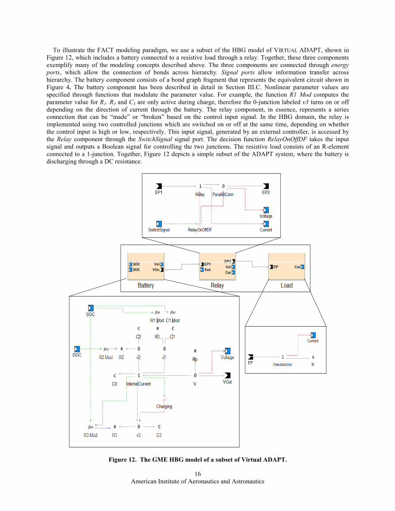
Figure 14. A fragment of the ADAPT Bayesian Net model.
Example: In Figure 14 we show a fragment of the ADAPT BN model M, focusing on a relay, a voltage sensor
and a current sensor associated with that relay. In terms of our formal framework discussed above, we have H(t) =
{HealthRelay, HealthVoSe, HealthCuSe}, C(t) = {CmdRelay}, P(t) = {SourcePath}, U(t) = {SinkPath}, M(t) =
{RelayStatus, Voltage, Current}, and S(t) = {SensorVo, SensorCu}.
The HealthRelay and CmdRelay nodes determine the RelayStatus of the relay, where RelayStatus is opened or
closed. The RelayStatus node again influences the SourcePath and SinkPath nodes, which represent whether there
are one or more open paths to the batteries and the loads respectively. SourcePath and SinkPath also depend on
other nodes in the BN, beyond the scope of this discussion. The SensorVo node represents the observed voltage of
the voltage sensor, while HealthVoSe represents its health status. In a similar way, SensorCu represents the observed
current of the current sensor, and HealthCuSe represents its health status. A crucial difference between voltage and
current sensors is that the former only depend on the existence of a path to one or more batteries, while the latter
also depend on the existence of a path to one or more loads. As a consequence, Current has two parents, SinkPath
and SourcePath, while Voltage has only one parent node, SourcePath. Finally, the sensor observations also depend
on health nodes HealthVoSe (health of voltage sensor) and HealthCuSe (health of current sensor).
We now consider diagnostic inference using the ADAPT BN. Suppose that the inputs to the BN are c(t) =
{Command = close} and s(t) = {SensorVo = high, SensorCu = low}, and suppose for simplicity that there is no other
evidence set in the BN. In other words, there is an inconsistency between the high voltage reading and the low
current reading. Suppose that we compute the marginal probabilities or the Maximum a posteriori (MAP)
probability over H(t); in this case the BN inference result is h(t) = {HealthVoSe = healthy, HealthRelay = healthy,
HealthCuSe = stuckLow}. This is reasonable, since it says that the likely cause of the low current reading in s(t) is
that the current sensor HealthCuSe is stuck low while the two other sensors are healthy.
The current Bayesian Network model M for ADAPT was developed in collaboration with Mark Chavira and
Adnan Darwiche of UCLA. For each time slice, the number of BN nodes in the ADAPT model is currently 344.
Note that the ADAPT BN is not created directly by a system designer. Instead, the designer creates a high-level

American Institute of Aeronautics and Astronautics
20
specification of an ADAPT BN model, and then that specification is translated into a BN which is then compiled,
using the tree clustering or arithmetic circuit approach, into a structure that is used for diagnosis and sensor
validation at run time. Using the Hugin§§ system with its default settings, the clique (or junction) tree size of the
ADAPT BN is found to be 4810. Using the Ace*** system with its default settings, the ADAPT BN is compiled into
an arithmetic circuit with 3,832 nodes, 5,624 edges, and 671 variables. For both systems, inference time without
evidence is less than 50 ms on a 1.83GHz Intel CPU with 1GB of RAM. This is very promising given ADAPT’s
sampling rate of 2Hz.
VI. Applications
ADAPT is being used by two high-level applications to study the process of deploying their specific
technologies on actual hardware in an operational setting. Development of caution and warning systems for future
aerospace vehicles is an important area of research to ensure the safe operation of these vehicles. The use of
automation of the underlying health management functions has the potential to cut operational costs and increase
safety. The benefits of using some of the same diagnostic models and analysis tools to improve the development of
contingency management procedures are also evident. These two applications are described in this section.
A. Advanced Caution and Warning System (ACAWS)
Most health monitoring on current aerospace vehicles results in caution and warning (C&W) signals that are
issued when logical rules are violated. The inputs to the rules are typically sensor values and contextual information,
such as the mission mode. When failures occur, in many cases a cascade of C&W alarms may be triggered. It is
necessary for the user to process the alarms and assess the situation in order to take appropriate corrective and safety
actions. Assistance is often required from expert operators. Many of the C&W alarms are daughter faults stemming
from a root cause and consequently are considered to be nuisance alarms. The introduction of more sophisticated
health management techniques has the potential to avoid the proliferation of messages by diagnosing the root cause,
thereby simplifying situational assessment and reducing the dependence on a large team of subsystem experts to
analyze the alarms.
But certain issues will need to be addressed before intelligent health management technologies become widely
adopted. An advantage of logical rules is that they are relatively easy to understand, implement, and test. For
reasoning algorithms that produce failure candidates, users will likely want to know whether and why those
candidates are valid. Additional questions arise when there are multiple candidates that seem to describe the current
system observations. If the actions to be taken are the same for all of the hypothesized failures, then the issue is
moot. However, if the actions taken for an assumed fault exacerbate the situation, when another fault in the
candidate list is the true cause, one might need to further disambiguate the failure candidates. In current systems,
C&W alarms are mapped to pre-defined procedures that the crew is expected to follow. Implicit in the mapping is
knowledge of the affected system functions. With advanced health management techniques this mapping from faults
to affected functions to recovery/mitigation/safing actions will have to be thoroughly reexamined.
To investigate concepts for advanced caution and warning systems, ADAPT has been connected to the
Intelligent Spacecraft Interface Systems (ISIS) at Ames. ISIS uses eye-tracking and a variety of human performance
measurement tools to assess the effectiveness of human-computer interactions. Graphical displays in ISIS present
data from ADAPT. Faults are injected in ADAPT and presented to the crew member with and without advanced
health management and display techniques. The goal is to determine the best way to integrate these technologies
into a fault management support system that assists the crew in all aspects of real-time fault management, from fault
detection and crew alerting through fault isolation and recovery activities.
To this end, we will be conducting a human-in-the-loop, hardware-in-the-loop experiment that will compare two
competing cockpit interface designs for a spacecraft fault management support system: Elsie and Besi. The design of
Elsie mimics a redesigned but never-implemented avionics interface for the Space Shuttle. The Cockpit Avionics
Upgrade (CAU) team was able to significantly improve the display of relevant information by reorganizing the data
based on a task analysis and presenting a graphical layout of components rather than only textual data. Elsie
provides the crewmember a schematic view of ADAPT, a more detailed, Shuttle-like textual display, and separate
displays for software commandable switch panels. Moreover, Elsie uses bounds checking for its C&W system in
which each out-of-limit condition is separately annunciated, without regard to its relationship to the fault. In
contrast, Besi extends the design philosophy of CAU displays by further increasing the use of graphics and analog
§§ http://www.hugin.com
*** http://reasoning.cs.ucla.edu/ace

American Institute of Aeronautics and Astronautics
21
representations of data and decreasing textual, digital representations of data. It also combines information display
with switch commanding onto a single schematic representation of ADAPT, enabling the crewmember to visualize
and reconfigure the system from a single display. Besi uses the HyDE diagnosis system described previously to
determine the root cause fault. It presents only this root cause fault to the crewmember and suppresses any
propagated faults.
In the first phase of the upcoming experiment, eight instrument-rated general aviation pilots will be tasked to
perform sixteen trials (runs) designed to evaluate the benefits and drawbacks of Elsie and Besi. Each trial will begin
with the same hardware configuration: battery A connected to load bus A and battery B connected to load bus B.
Both load buses will power two critical systems and two non-critical systems. In the experiment, these systems
represent Environmental Control and Life Support systems, although in reality they are lights and pumps.
Additionally, load bus A will have distinct but functionally-equivalent systems as the two critical systems connected
to load bus B and vice versa. In the initial configuration, these backup systems will be connected but not powered.
Each trial will introduce either one or two faults into this initial configuration, repeated once with the pilot using
Elsie as the interface to the fault management system and again with the pilot using Besi. The trials are counter-
balanced and the fault scenarios are designed to decrease learning-effect as much as possible. The complete
experiment design details are outside the scope of this paper but are available on request.
The eight fault scenarios to be tested in the trials are shown in Table 5. In brief, the scenarios include either a
single fault or two faults injected serially after a delay, and span a range of complexity. Our goal is to determine not
only whether one interface is overall faster or preferred by pilots, but also under what conditions any benefits and
drawbacks arise. We aim to accomplish this by using techniques that assess performance at several levels of
behavioral specificity and temporal granularity, from performance across an entire trial, through performance on
distinct phases within a trail (e.g., detecting a problem, diagnosing the cause, selecting a recovery procedure,
executing the procedure), and finally down to performance on each of the most basic elements of each activity (e.g.,
hear the alarm, find the alarm on the screen, turn off the alarm).
B. Contingency Analysis
Some aerospace projects focus development efforts on the normal behavior required of the system to such an
extent that consideration of failure scenarios is deferred until after design implementation. A contingency is an
anomaly that must be handled during operations. Fault protection systems in spacecraft are an example of
contingency handling software, automating the response of a spacecraft control system to anomalies during
operation. Contingency handling defines requirements for detecting, identifying, and responding to anomalous
events. A process for contingency analysis during design has been developed29 and is being implemented in the
ADAPT domain. The approach involves two steps: (1) to integrate in a single model the representation of the
contingencies and of the data signals and software monitors required to identify those contingencies and (2) to use
tool-supported verification of the diagnostics design to identify gaps in coverage of the contingencies.
Building the system model with faults integrated into it, rather than later composing a system model with a
separately-developed fault model, simplifies designing for contingencies. System modeling using TEAMS Designer
integrates in one model the identified contingencies and the signals and monitors needed to identify those
contingencies. The modeling in TEAMS consists of the following tasks:
(1) Identify the system’s architectural components and connectors associated with the system’s key
functionality. The connectors show the data signals that modules can use to identify whether contingencies
have occurred. Note that the links along which data signals propagate also trace the dependencies among the
modules.
(2) For each module, identify the contingencies (anomalous events or states) that can obstruct the system from
achieving its goal.
(3) Identify the checks or monitors, called tests in TEAMS, by which the contingencies of concern can be
detected. Requirements on the ordering of the tests can be modeled in TEAMS by specifying the level of
each test. This is especially useful for ensuring that the most-likely diagnoses will be examined first.
Recovery actions to handle identified contingencies can also be represented in TEAMS.
(4) Identify the architectural test-points for each of these monitors. These test-points are placed in the model at
the positions where checks can be run to detect failures or other contingencies.
The ADAPT model under development for the performance assessment of diagnostic approaches is being used
in this analysis of contingency handling design. The “Monitor_Control” block shown in Figure 8 will be expanded
so that more of the system control aspects can be included in this analysis. Currently, that block contains only the
monitoring points organized by the backplanes enumerated in Table 1. At this level, contingencies resulting from the

American Institute of Aeronautics and Astronautics
22
failure of data acquisition hardware (a module or backplane) can be studied and a system design developed so that
system reconfiguration strategies include the assignment of critical functions to multiple modules.
Table 5. ACAWS fault scenarios.
Scenario
Number
Scenario Description (serial faults are designated as (a) then (b))
Scenario Explanation
& Evaluation Objective
1 Switch to a critical load (i.e., sensor on ECLSS
component) fails open (either the switch fails or
the switch sensor fails)
We are deliberately providing an incomplete
model to HyDE to prevent it from correctly
diagnosing the false alarm. Whether the switch or
the sensor fails, HyDE will deduce that the switch
failed. Evaluating performance on an actual
failure and a false alarm allows us to determine
whether pilots will implicitly trust the automation
or will verify its diagnoses.
2 (a) Connection to a load bus fails open (false
alarm), then (b) a critical load-level sensor fails
(either actually or false alarm) on the other load
bus.
Similar to scenario 1, but the first annunciated
fault increases workload. This allows us to
determine whether the benefits of an interface
increase with workload increase.
3 Connection between battery & load fails open
transiently (it can be restored with a switch
recycle).
Allows us to evaluate the interfaces in a simple,
perhaps typical, fault environment (single fault,
low workload).
4 (a) Battery voltage fails low, then (b) one of the
switches that connects that battery to a load fails
open.
The second fault is irrelevant to the recovery
process; the switch state is irrelevant because the
first fault made that battery unusable. This helps
us determine how pilots will treat faults of
irrelevant components.
5 An inverter fails off. Critical loads will be lost on the affected load bus.
This helps us determine the benefits of an
interface under a high time criticality condition.
6 (a) One of the redundant sensors on a critical AC
load fails low, then (b) the inverter on the other
load bus fails off.
The first fault is much lower priority than the
second fault. This helps us determine any
associated benefits of an interface for assisting
with assessment and management of priorities.
7 (a) An inverter fails off, then (b) the circuit
breaker to the critical load on the DC bus fails
open.
Both faults are equally critical. This helps us
determine the effectiveness of an interface in
helping pilots deal with equal priority faults.
8 (a) Connected battery (either battery A or B)
voltage fails low, then while the recovery
procedure (connect the affected load to the spare
battery) is being implemented (b) the spare
battery (battery C) voltage fails low.
The initial recovery procedure will not restore
necessary functionality and the pilot will need to
determine a new course of action. (In this case,
rather than switching to the spare battery, they
would need to turn on the backups for the critical
systems attached to the remaining battery (battery
B or battery A).) This helps us determine the
effectiveness of an interface in helping pilots
adjust mitigation tactics.
Identifying undetectable contingencies
TEAMS Designer models a system as a directed graph and internally runs a reachability analysis to determine
which faults (or other contingencies) can be detected at each test point.††† An example of this analysis for ACAWS
fault scenario 3 is shown in Figure 15. A testability analysis is performed on the ADAPT model and the fault mode
representative of scenario 3 is selected. The model is then highlighted (indicated by a blue box) to show the
monitoring points that are active in isolating that failure model. To achieve this, TEAMS builds a dependency
††† Qualtech Systems, Inc., http://www.teamqsi.com/
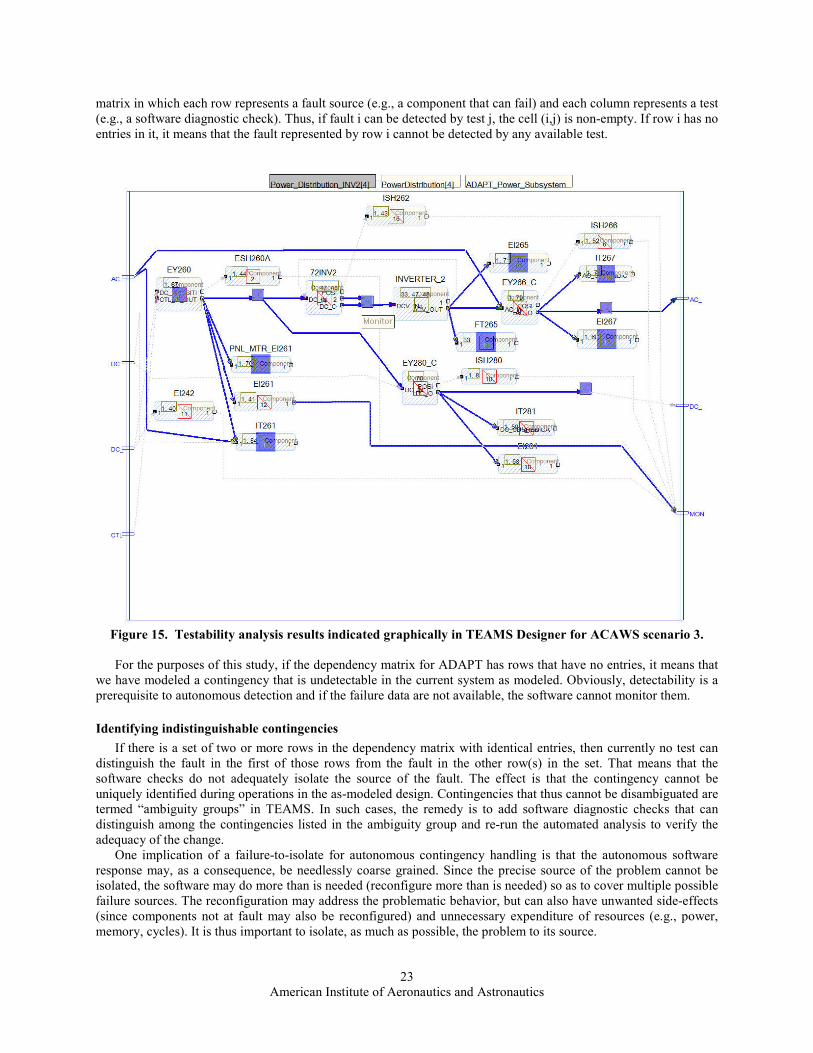
American Institute of Aeronautics and Astronautics
23
matrix in which each row represents a fault source (e.g., a component that can fail) and each column represents a test
(e.g., a software diagnostic check). Thus, if fault i can be detected by test j, the cell (i,j) is non-empty. If row i has no
entries in it, it means that the fault represented by row i cannot be detected by any available test.
Figure 15. Testability analysis results indicated graphically in TEAMS Designer for ACAWS scenario 3.
For the purposes of this study, if the dependency matrix for ADAPT has rows that have no entries, it means that
we have modeled a contingency that is undetectable in the current system as modeled. Obviously, detectability is a
prerequisite to autonomous detection and if the failure data are not available, the software cannot monitor them.
Identifying indistinguishable contingencies
If there is a set of two or more rows in the dependency matrix with identical entries, then currently no test can
distinguish the fault in the first of those rows from the fault in the other row(s) in the set. That means that the
software checks do not adequately isolate the source of the fault. The effect is that the contingency cannot be
uniquely identified during operations in the as-modeled design. Contingencies that thus cannot be disambiguated are
termed “ambiguity groups” in TEAMS. In such cases, the remedy is to add software diagnostic checks that can
distinguish among the contingencies listed in the ambiguity group and re-run the automated analysis to verify the
adequacy of the change.
One implication of a failure-to-isolate for autonomous contingency handling is that the autonomous software
response may, as a consequence, be needlessly coarse grained. Since the precise source of the problem cannot be
isolated, the software may do more than is needed (reconfigure more than is needed) so as to cover multiple possible
failure sources. The reconfiguration may address the problematic behavior, but can also have unwanted side-effects
(since components not at fault may also be reconfigured) and unnecessary expenditure of resources (e.g., power,
memory, cycles). It is thus important to isolate, as much as possible, the problem to its source.

American Institute of Aeronautics and Astronautics
24
Identifying redundant diagnostic checks
The TEAMS tool also detects cases in which redundant tests exist for a single contingency. This may indicate
inefficiency in the contingency detection software or it may indicate that the intent differs from the actual system. Of
course, the model could also be wrong, so iterative review by project experts is a key step in the process.
ADAPT is being used to study this process for contingency verification using the model developed for the
diagnostic application. The troubleshooting tree will be generated and the ACAWS scenarios will serve as a baseline
set of actions that should be taken when those specific faults occur. The model will be augmented with steps in the
recovery plans and the automatically-generated tree will be compared to the manually generated procedures. This
application will serve to evaluate the process on a larger system than that which was used during the development of
the process.
VII. Performance Assessment
The purpose and scope of assessments and experiments as they relate to diagnostic and prognostic techniques
and systems can vary significantly. We now identify a few different classes of assessments.
I. Platform assessment: Processors (CPUs) and operating systems may react differently to different diagnostic
workloads. Therefore, it can be of interest to test an implementation on different computational platforms.
II. Implementation assessment: The programming language and the data structures can have a substantial
impact on performance; hence it may be of interest to compare different implementations of the same
algorithm.
III. Algorithm assessment: Different algorithms may solve the same computational problem. For instance, the
problem of computing marginals in Bayesian networks can be solved using clique tree clustering or other
approaches. Typically, this type of assessment involves the use of problem instances.24
IV. Technique assessment: The problem of electric power system diagnosis can be addressed using, for
example, Bayesian networks or artificial neural networks. This is discussed in Section V.
V. System assessment: Overall system performance may also depend on the human(s) in the loop, and how they
use and interact with different automated diagnostics systems. This is discussed in Section VI.
Initial efforts will focus on classes III, IV, and V. The assessment of different diagnostic algorithms will consist
of metrics determined from the compilation of several test runs, which include nominal and faulty behavior. For a
single test run, it will be classified as a false alarm if a fault was not injected during the run but the test article
reported one or if the test article reported a fault before it was injected. If the test article does not report a fault when
one was injected, it will be classified as a missed alarm. The correctness and precision of fault isolation will also be
determined for each run. By combining the results over several runs, false alarm rates, missed alarm rates, and
isolation rates for the test article will be measured. Additional metrics include fault detection and isolation times.
Not all of the metrics will apply to each test article. For example, a particular technique may only perform fault
detection without isolating the cause of the fault.
The eight scenarios described in Table 5 were selected for the first set of analysis runs. These scenarios are not
particularly difficult for the diagnostic reasoners but will provide a standard set of faults and system responses for
experimenting with the parameters of the reasoning algorithms. Each reasoning approach will be studied in detail; it
is important not only to get the correct diagnosis – the intermediate steps taken by each algorithm will be studied in
detail. Later runs will include input data variations such as limited sensor inputs, i.e., only data from voltage sensors
will be available or some data that is available intermittently. Consistency will be maintained as much as possible
across the test articles.
VIII. Conclusion
This paper describes a testbed at NASA Ames Research Center for evaluating and maturing diagnostic and
prognostic concepts and technologies. The electrical power system hardware together with the software architecture
and unique concept of operations offers many challenges to diagnostic applications such as a multitude of system
modes, transient behavior after switching actions, multiple faults, and load-dependent noise. A simulation model is
available to facilitate the development and testing of health management applications. Future work will include the
integration of more test articles, loads, faults, operational scenarios, and evaluation techniques. In meeting the five
goals of the testbed listed in Section I, much greater knowledge of the trade-offs among diagnostic technologies will
be available to system designers for future programs. Many current technology assessments have relied upon trade
literature or technical publications of an algorithm’s definition and performance. ADAPT provides a technology-
neutral basis for the comparison of various techniques and a highly configurable operational environment for the
evaluation of an algorithm’s performance under specific operational requirements and fault conditions.

American Institute of Aeronautics and Astronautics
25
Acknowledgments
The authors would like to thank Lee Brownston for his detailed review and comments of the final versions of
this paper and Sriram Narasimhan for his contributions to Section V.B. We also thank Somnath Deb, Sudipto
Ghoshal, Charles Domagala and Venkat Malepati from Qualtech Systems, Inc. for creating the TEAMS model of
ADAPT under NASA contract number NNA06AA51Z and the TEAMS-RT application for the testbed under NASA
contract number NNA06AA64C, and for their many discussions on the design of the diagnostic experiments.
Contributions by RIACS were based upon work supported by NASA under award NCC2-1426. Contributions by
Perot Systems were supported by NASA under contract NNA04AA18B and contributions by SAIC were supported
by NASA under contract NAS2-02091. Contributions by Vanderbilt University were supported by NASA USRA
grant 08020-013, NASA NRA grant NNX07AD12A, and NSF CNS-0615214. The contributions by the Jet
Propulsion Laboratory, California Institute of Technology, were carried out in part under a contract with NASA and
funded by NASA’s Office of Safety and Mission Assurance through the IV&V Facility. Dr. Lutz’s research is also
supported by NSF grant 0541163. Finally, we also thank and acknowledge the efforts of the ACAWS team
members: Mark Anderson, Durand Begault, Brent Beutter, Steve Elkins, Miwa Hayashi, Rob McCann, Fritz
Renema, and William Taylor.
References 1Karsai, G., Biswas, G., Abdelwahed S., Narasimhan S., Pasternak T., and Szemethy T., “Towards Fault-Adaptive Control of
Complex Dynamic Systems”, Software Enabled Control, IEEE Press, 2003. 2Manders, E. J., Biswas, G., Mahadevan, N., and Karsai, G., “Component-Oriented Modeling of Hybrid Dynamic Systems
using the Generic Modeling Environment,” Proceedings of the 4th Workshop on Model-Based Development of Computer Based
Systems, 2006. 3Ledeczi, A., Maroti, M., Bakay, A., Nordstrom, G., Garrett, J., Thomason IV, C., Sprinkle J., Volgyesi P., GME 2000 Users
Manual (v2.0), December 18, 2001. 4Ledeczi, A., Balogh, G., Molnar, Z., Volgyesi, P., Maroti, M., “Model Integrated Computing in the Large,” IEEE Aerospace
[CD Rom], Big Sky, MT, March 6, 2005. 5Karsai, G., Sztipanovits, J., Ledeczi, A., and Bapty, T., “Model-Integrated Development of Embedded Software,”
Proceedings of the IEEE, Volume: 91, Issue: 1, Jan. 2003, pp. 145-164. 6Mosterman, P. J., and Biswas, G., “A Theory of Discontinuities in Physical System Models,” J Franklin Institute, vol. 335B
(3):401-439, 1998. 7Karnopp, D. C., Margolis, D. L., and Rosenberg, R. C., Systems Dynamics: Modeling and Simulation of Mechatronic
Systems, New York: John Wiley & Sons, Inc., 3rd edition, 2000. 8Biswas, G., Simon, G., Mahadevan, N., Narasimhan, S., Ramirez, J., and Karsai, G., “A Robust Method for Hybrid
Diagnosis of Complex Systems,” 5th IFAC Symposium on Fault Detection, Supervision and Safety of Technical Processes
(SAFEPROCESS), Washington, D.C., June 2003, pp. 1125-1130. 9Narasimhan, S., and Biswas, G., “Model-Based Diagnosis of Hybrid Systems”, IEEE Transactions on Systems, Man, and
Cybernetics, Part A, 37(3):348-361, 2007. 10Abdelwahed, S., Wu, J., Biswas, G., Ramirez, J., and Manders, E., "Online Fault Adaptive Control for Efficient Resource
Management in Advanced Life Support Systems," The International Journal for Human Support Research, vol. 10, no. 2, 2005,
pp. 105-115. 11Roychoudhury, I., Daigle, M., Biswas, G., Koutsoukos, X., and Mosterman, P. J., “A Method for Efficient Simulation of
Hybrid Bond Graphs,” Proceedings of the International Conference on Bond Graph Modeling (ICBGM 2007), 2007, pp. 177-
184. 12Daigle, M., Roychoudhury, I., Biswas, G., and Koutsoukos, X., “Efficient Simulation of Component-Based Hybrid Models
Represented as Hybrid Bond Graphs,” Technical Report ISIS-06-712, Institute for Software Integrated Systems, Vanderbilt
University, Nashville, TN, USA, 2006. 13Ceraolo, M., “New Dynamical Models of Lead-Acid Batteries,” IEEE Transactions on Power Systems 15(4):1184-1190,
2000. 14Deb, S., Pattipati, K. R., Raghavan, V., Shakeri, M., and Shresta, R., “Multi-Signal Flow Graphs: A Novel Approach for
System Testability Analysis and Fault Diagnosis,” Proceedings of AUTOTESTCON ’94, 1994. 15Deb, S., Mathur, A., Willitt, P., and Pattipati, K., “De-centralized Real-Time Monitoring and Diagnosis,” IEEE
Transactions on Systems, Man, and Cybernetics, 1998. 16Hayden, S., Oza, N., Mah, R., Poll, S., Shirley, M., Mackey, R., Narasimhan, S., Karsai, G., and Deb, S., “Diagnostic
Technology Evaluation Report for On-board, Crew Launch Vehicle,” NASA/TM-2006-214552, 2006. 17Narasimhan, S., Dearden, R., and Benazera, E., “Combining Particle Filters and Consistency-Based Approaches for
Monitoring and Diagnosis of Stochastic Hybrid Systems,” 15th International Workshop on Principles of Diagnosis (DX04),
Carcassonne, France, 2004.

American Institute of Aeronautics and Astronautics
26
18Mosterman, P. J., and Biswas, G., “Diagnosis of Continuous Valued Systems in Transient Operating Regions,” IEEE
Transactions on Systems, Man and Cybernetics, Part A 29(6):554-565, 1999. 19Gelb, A. Applied Optimal Estimation. Cambridge, MA, USA: MIT Press, 1979. 20Narasimhan, S., Biswas, G., Karsai, G., Pasternak, T., and Zhao, F., “Building Observers to Address Fault Isolation and
Control Problems in Hybrid Dynamic Systems,” IEEE Transactions on Systems, Man, and Cybernetics, Volume 4, 8-11 Oct.
2000, pp. 2393-2398. 21Mengshoel, O. J., “Designing Resource-Bounded Reasoners Using Bayesian Networks: System Health Monitoring and
Diagnosis,” Proceedings of the 18th International Workshop on Principles of Diagnosis (DX-07), Nashville, TN, (to be
published). 22Lauritzen, S. L., and Spiegelhalter, D. J., “Local Computations with Probabilities on Graphical Structures and Their
Application to Expert Systems,” Journal of the Royal Statistical Society, 50(2):157-224, 1988. 23Shenoy, P. P., and Shafer, G., “Axioms for Probability and Belief-Function Propagation,” Proceedings of the Fourth
Annual Conference on Uncertainty in Artificial Intelligence, 1990, pp. 169-198. 24Mengshoel, O. J., Wilkins, D. C., and Roth, D, “Controlled Generation of Hard and Easy Bayesian Networks: Impact on
Maximal Clique Tree in Tree Clustering,” Artificial Intelligence, 170(16-17):1137-1174, 2006. 25Mengshoel, O. J., “Macroscopic Models of Clique Tree Growth for Bayesian Networks,” Proceedings of the 22nd AAAI
Conference on Artificial Intelligence (AAAI-07). July 22-26, 2007, Vancouver, British Columbia, Canada (to be published). 26Darwiche, A., “A Differential Approach to Inference in Bayesian Networks,” JACM, 50(3):280-305, 2003. 27Huang, J., Chavira, M., and Darwiche, A., “Solving MAP Exactly by Searching on Compiled Arithmetic Circuits,”
Proceedings of the 21st National Conference on Artificial Intelligence (AAAI-06), July 2006, Boston, MA, pp. 143-148. 28Chavira, M., and Darwiche, A., “Compiling Bayesian Networks Using Variable Elimination,” Proceedings of the 20th
International Joint Conference on Artificial Intelligence (IJCAI-07), Hyderabad, India, January 2007. 29Lutz, R., Patterson-Hine, A., Nelson, S., Frost, C., Tal, D., and Harris, R., “Using Obstacle Analysis to Identify
Contingency Requirements on an Unpiloted Aerial Vehicle”, Requirements Engineering Journal, 12(1), 2007, pp. 41-54. 30Ghoshal, S., Azam, M., and Malepati, V., SBIR Phase III "Comprehensive Fault Detection, Isolation, and Recovery (FDIR)
on the ADAPT Test Bed," Progress Report 1, Contract No. NNA06AA51Z, Oct. 2006.