This article appeared in a journal published by Elsevier. The attachedcopy is furnished to the author for internal non-commercial researchand education use, including for instruction at the authors institution

and sharing with colleagues.

Other uses, including reproduction and distribution, or selling orlicensing copies, or posting to personal, institutional or third party

websites are prohibited.

In most cases authors are permitted to post their version of thearticle (e.g. in Word or Tex form) to their personal website orinstitutional repository. Authors requiring further information

regarding Elsevier’s archiving and manuscript policies areencouraged to visit:

http://www.elsevier.com/copyright

Author's personal copy

Evaluation of soil water content in tilled and cover-cropped olive orchards by thegeoelectrical technique

G. Celano a, A.M. Palese a,⁎, A. Ciucci b, E. Martorella c, N. Vignozzi d, C. Xiloyannis a

a Dipartimento di Scienze dei Sistemi Colturali, Forestali e dell'Ambiente, Università degli Studi della Basilicata, Viale dell'Ateneo Lucano, 10, 85100 Potenza, Italyb Geostudi Astier s.r.l., Via della Padula, 165, 57124 Livorno, Italyc Studio GEDIT, Geologia per l'Edilizia ed il Territorio, Via Manfriana, 18, 87012, Castrovillari (CS), Italyd CRA, ABP, Centro di Ricerca per l'Agrobiologia e la Pedologia, Piazza M. D'Azeglio, 30 50121 Firenze, Italy

a b s t r a c ta r t i c l e i n f o

Article history:Received 1 July 2010Received in revised form 10 March 2011Accepted 27 March 2011Available online 20 May 2011

Keywords:Olea europaea L.Soil managementCover cropsSoil electrical resistivityVolumetric soil water contentSoil water reserve

Electrical Resistivity Imaging (ERI) was performed in southern Italy, under semi-arid climate, on a HaplicCalcisol soil of two rainfed olive orchards managed according to different soil management (Tillage – T, andCover Cropping – CC), applied for 8 years. The main aim was to test the usefulness of such geoelectricalmethod for the assessment of spatial and temporal variability of soil water content for water balance studies.For that purpose, the quality of univariate relationships between soil electrical resistivity (ρ) and volumetricsoil water content (θv) was tested.Three geoelectrical measurement campaigns were performed in the autumn–spring period of 2006–2007. Foreach campaign, 3 two-dimensional (2-D) geoelectrical tomographies were carried out in the pole–dipolearray using a fixed electrode spacing of 0.25 m. 2-D apparent resistivity pseudosection data sets have beeninverted using the software TomoLab®. Each covered soil section was 3 m in depth and 11.5 m long. On 14November 2006 and 18 April 2007 campaigns the ERI were followed by soil samplings carried out with augerdirectly below the respective geoelectrical profiles. Direct measurements of soil electrical conductivity andsoil water content were conducted on the soil samples in situ and in the laboratory.Volumetric soilwater content, θv (mmmm−1), was significantly related to soil electrical resistivity data, ρ (Ωm),by the exponentialmodel θv=1.641ρ−0.599 (R=0.866,n=84). This relation allowed to assess the change of soilwater content in the two orchards during the autumn–spring period and to reveal that the CC plot was moreefficient to intercept and store rainwater. ERI technique allowed to highlight differences between the systems inthe dynamics ofwater distribution along the soil profile as aneffect of the adopted soilmanagement. Inparticular,such technique consented to easily evaluate the extent of water content of the deepest soil layers (N1.0 m)evidencing a significant water reserve in the CC plot, convenient for the root system of rainfed olive trees in thedriestmonths. Finally, the soilwater content evaluatedbymeans of theERI techniquewasused for the short-termapplication of soilwater balancewhich showed interesting data on theprogress ofwater consumption during theautumn–spring period, particularly useful as operative indications for cover crops management.

© 2011 Elsevier B.V. All rights reserved.

1. Introduction

The implementation of sustainable practices in agriculture is oneof the main strategies adopted by many countries in the world tocontrast problems such as water shortage, desertification, greenhouseeffect and pollution, which are threatening the environment and thehuman welfare.

Sustainable soil management technologies (i.e. ground cover bysown or spontaneous vegetation) play a fundamental role in fruitgrowing because they are aimed a) to improve and/or maintain soilorganic matter as a key factor of physical, chemical, andmicrobiological

soil quality; b) to prevent soil erosion; c) to increase biodiversity andecosystem stability; d) to improve CO2 sequestration from theatmosphere by orchard systems Furthermore, in arid and semi-aridenvironments, where water is the most limiting factor for cropproduction under dryland farming, a correct water resource manage-ment requires a large knowledge of the spatial variability of soilproperties (particularly, soil structure and hydraulic properties) whichstrongly affect the water balance (Srayeddin and Doussan, 2009).

Traditionally, soil characteristics and their spatial variations arequantified using destructive, laborious, and time-consuming directmeasurements on a wide number of soil samples which are subjectedto large errors (Amato et al., 2008; Böhm, 1979, Celano et al., 2010;Hagrey and Michaelsen, 2002; Lazzari, 2008; Samouëlian et al., 2005).

Otherwise, non-invasive geophysical techniques, such as ElectricalResistivity Imaging (ERI), can be rapidly and easily performed over

Geoderma 163 (2011) 163–170

⁎ Corresponding author. Tel.: +39 0971 205267, +39 347 0055234(mobile);fax: +39 0971 205378.

E-mail address: assunta.palese@unibas.it (A.M. Palese).

0016-7061/$ – see front matter © 2011 Elsevier B.V. All rights reserved.doi:10.1016/j.geoderma.2011.03.012

Contents lists available at ScienceDirect

Geoderma

j ourna l homepage: www.e lsev ie r.com/ locate /geoderma

Author's personal copy

wide areas to describe horizontal and vertical variability of soilstructure and properties at the scale of interest also by geostatisticalapproach (Tabbagh et al., 2000; Besson et al., 2010). The electricalresistivity can be affected by root systems and different soilcharacteristics. Hence, geoelectrical surveys are often aimed toestablish relationships between the resistivity values and the othersoil features (texture, water content, solute concentration). In thecontext of soil science, electrical resistivity allows the delineation ofthe main soil types and, when performed repeatedly over time, alsoprovides information on soil functioning. The information collected isvery useful for agronomists, soil scientists, civil and environmentalengineers, and supports them in the sustainable management ofnatural resources (Samouëlian et al., 2005; Celano et al., 2010).

Also in very heterogeneous tree orchard systems, ERI technique isable to map the whole rooting zone, the moisture and salinityvariations, the water flows of the soils investigated starting fromelectrical measurements carried out on the surface (Celano et al.,2010; Hagrey and Michaelsen, 2002; Lazzari, 2008).

Geoelectrical surveys are based on the measurement of thedistribution of electrical currents induced by an applied electricfield. The development of the electrical potential field depends on theresistivity distribution in the subsurface. The measurements are oftendisplayed as two-dimensional pseudosections, that provide thespatial distribution of apparent resistivity. The distribution of thetrue resistivity can be obtained from numerical inversion (Samouëlianet al., 2005).

In the present study, the non-destructive ERI technique, combinedwith conventional methods of soil investigation, was applied toheterogeneous olive orchard systems on tilled and cover croppedsoils. This combined application was aimed to verify a) the quality ofunivariate relationships between soil electrical resistivity (ρ) andvolumetric soil water content (θv); b) the use of the geoelectricaltechnique as a tool for the assessment of spatial and temporalvariability of soil water content.

2. Materials and methods

2.1. The experimental set up

The experiment was performed in a mature olive grove located insouthern Italy (Ferrandina – Basilicata Region, 40°29′ N, 16°28′ E)grown under rainfed conditions. Olive trees (Olea europaea L. – cvMaiatica, a double aptitude variety)were vase trained and planted at adistance of about 8×8 m.

From 2000, the olive orchard was divided into two plots managedaccording to different soil management systems: cover cropping (CC)and tillage (T). The soil surface of the CC plot was permanentlycovered by spontaneous weeds, mowed at least twice a year. In the CCplot trees were lightly pruned each year. Crop residues and pruningmaterial were left on the ground asmulch. Tilled plot wasmanaged bycontinuous tillage (milling at 10 cm soil depth) not to have any weedson the soil during the studied period. Heavy pruning was carried outevery two years, but pruned residues were burned out of the olivegrove.

2.2. Climatic and pedological characterisation of the experimental site

The climate in the area is classified as semi-arid, with an annualrainfall of 561 mm (mean 1976–2006). The mean annual temperatureranges from 15 to 17 °C.

The key meteorological parameters (air temperature, rainfall,humidity, etc.) were measured daily by a standard weather stationplaced close to the trial area. The reference evapotranspiration (ETo),provided by SAL service of the Extension Regional Service (www.alsia.it), was the mean value coming from the application of the followingmethods for ETo estimation: Blaney–Criddle, radiation, and Hargreaves.

The soil of the experimental grove is a sandy loam classified as aHaplic Calcisol (FAO, WRB, 1998) with Ap1 (0.0–0.30 m) /Ap2 (0.30–0.50 m)/Bk (0.50–1.00 m)/Ck (1.00–2.00 m) profile. It has a lowgravel content and shows an increasing concentration of finelydivided calcium carbonate particles in the soil matrix passing fromthe surface horizons (Ap soil horizons, 0.0–0.50 m) to the parentalmaterial (Ck, soil layerN0.6 m). CC and T plots belongs to the same soilunit as verified by two pedological profiles. Soil characteristics of theCC and T plots are reported in Table 1.

2.3. Soil resistivity measurements and Electrical Resistivity Imaging (ERI)

Three geoelectrical measurement campaigns were carried out inboth systems, CC and T. They were performed in the autumn–winterperiod at the following dates: 14 November 2006, 9 January 2007, and18 April 2007. In each survey date, three 2D geoelectrical tomogra-phies were performed in both the systems, studying an area of 576 m2

per plot. Data were collected using an Iris Syscal Pro resistivity meter(ten-channel receiver) connected to a 12 V battery that resulted in aDC current amplified at 100 V. A total of 48 electrodes pergeoelectrical measurement, 0.25 m spaced, were used. These specifictwo-dimensional (2-D) quadripolar pole–dipole sequences weredesigned to achieve an appropriate depth of investigation (soilprofile: from 0.0 to 3.0 m). 2-D inversions of soil apparent resistivity(ρa, Ω.m) and their graphic representation were performed using theTomoLab® software. Particularly, such software has been tested in alot of different conditions and for different applications and the resultsare generally accepted (Ribolini et al., 2010). TomoLab® software usesa finite-element algorithm in order to reconstruct the resisitivitydistribution. This approach, although slow and machine intense,allows a fine tuning of the inversion process, useful to appreciatesmall variation in soil resistivity. Information about specific charac-teristics of the above mentioned software is reported in LaBrecqueet al. (1996) and Morelli and LaBrecque (1996).

2.4. Soil sampling and analysis

After the geoelectrical surveys, representative set of soil sampleswere taken directly below the geoelectrical profiles in the CC and Tplots taking into account the different soil horizons (Ap1, Ap2, Bk, Ck).A total of 84 samples were collected during the field measurements of14th of November 2006 and 18th of April 2007 at different soil depths(from 0.0 to 2.5 m, step 0.10 m) by means of a pneumatic driller or amanual auger opening holes of 40 mm. Such sampling scheme wasfollowed in order to have a consistent number of cases and a detailedpicture of the soil water distribution.

Soil volumetric water content (θv, mm mm−1) was obtainedmultiplying the gravimetric water content (θw, g g−1) by the soil bulkdensity (Gardner, 1986).

Electrical conductivity (EC1:2.5) was measured in the laboratoryaccording to Rhoades (1982) by a Crison 525 conductivimeter (Crison,Barcelona) on a thoroughly shaken mix of soil (1.0 g dry weight ) anddistilled water (2.5 mL).

2.5. Statistical analysis

Field and laboratory data were splitted in three groups in relationto the pedological conditions and the studied systems as follow: I)data coming from parent material horizon (Ck) for both systems, CCand T; II) data coming from A+B horizons of the CC plot; III) datacoming from A+B horizons of the T plot.

In order to identify univariate association between ρ and θv,different statistical models were tested for each data group. Statisticalregression analysis, showing minimization of the sum of squareresiduals, normal distribution of the data residues, and the highestsignificativity of coefficients, was selected.

164 G. Celano et al. / Geoderma 163 (2011) 163–170

Author's personal copy

Statistical analysis was performed using STATISTICA® 6.0 (Stat-Soft, Inc.; www.statsoft.com).

2.6. Water consumption assessment

Estimation of water consumption (ETc) by the studied systems, CCand T, was carried out using the soil water balance approach(Fernández and Moreno, 1999) ETC was calculated by the followingEq. (1):

ETc ¼ R þ I� Δθv�D� Rs ð1Þ

where R (mm) is the rainfall, I (mm) the water applied by irrigation,Δθv (mm) the variation in the examined period of the water stored inthe soil profile exploited by the roots, ±D (mm) the water lost bydrainage or gained by rising groundwater, and Rs (mm) the surfacerunoff. In our case, the equation was simplified to Eq. (2)

ETc ¼ R � Δθv ð2Þ

because the experimental olive orchard was grown under rainfedconditions, the water table (8.0 m deep) remained far below themaximum depth of the root system (2.0 m), as evaluated by somepreliminary geoelectrical surveys and measurements of the waterlevel of the wells placed near the experimental field. Finally, it wasassumed that runoff was negligible because the slope of theexperimental plots was less than 2%. Δθv data were estimated bythe geoelectrical measurements performed in the three differentcampaigns along the 2006–2007 autumn–winter period, as describedbefore.

3. Results and discussion

3.1. Soil resistivity (ρ) vs volumetric soil water content (θv)

Regression model obtained from field and laboratory data splittedin three groups in relation to the soil horizons and the treatments arereported in Table 2. The statistical model that best described therelationship between ρ and θv was the exponential one Eq. (3)

ρ ¼ β1 × θβ2v ð3Þ

The exponential model was the same for the three groups eventhough it presented different coefficients depending on the highspecificity of the geoelectrical techniquewhich is able to investigate athorizon level (Table 2). Such condition leads us to try the use of aunique estimating relationship which did not take into account thepedological structure and the soil management systems. In order toevaluate the error linked to the use of a unique relationship under thedifferent conditions, all field and laboratory data (n=84) wererandomly splitted in two dataset by simple random sampling without

replacement: a training dataset (dataset I, n=57) and a validationdataset (dataset II, n=27). The regression of θv on ρ obtained fromdataset I was tested on dataset II. Values of measured ρ in datasetII (ρm) were used to estimate θv (θve) by the following exponentialmodel Eq. (4):

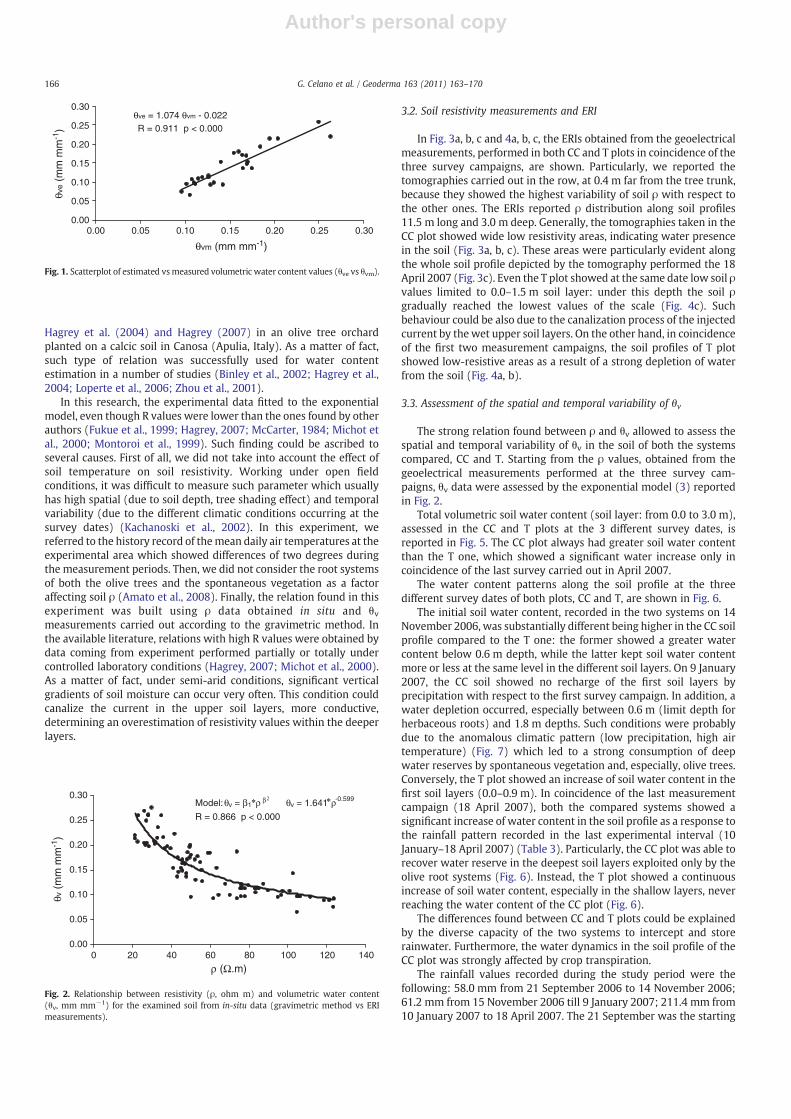
θve¼ β1 × ρβ2m ð4Þwhere the parameters named β1 and β2, coming from dataset Iregression, had values of 1.503 and −0.571, respectively. Theestimated θve values were then regressed on θvm values and θve–θvmpairs were compared by the Wilcoxon signed-rank test. The errorlinked to θv evaluation of dataset II samples by means of therelationship built on dataset I was very low and not statisticallydifferent according to theWilcoxon signed-rank test. When applied todataset II (n=27), the regression equation obtained from dataset I(n=57) yielded θve values that were highly correlated (pb0.001,n=27) with θvm values (Fig. 1), and were not significantly differentaccording to the Wilcoxon signed-rank test. According to theseevaluations, spatial and temporal variability of soil volumetric watercontent was estimated using the exponential model Eq. (3) resultingfrom the statistical relationship between all ρ and θv data (n=84)(Fig. 2; Table 2).

The electrical resistivity is a function of a number of soil propertiesnamely texture, water content and salinity (Samouëlian et al., 2005).Soil resistivity decreases when the water content, clay fraction andsalinity increase (Hagrey et al., 2004; Lazzari, 2008; Samouëlian et al.,2005). In particular, the conduction of electrical current in sandy soilsis mainly electrolytic, based on the displacement of ions in thesolution circulating in the pores of the soil, and therefore it is higherwith the presence of dissolved salts. Thus, the electrical current insoils depends both on the amount of water in the pores and on waterquality. Under the experimental conditions, the soil, characterized bya sandy texture (clay content lower than 15%,), showed low electricalconductivity values and light spatial variability of the soil character-istics (Table 1), so ρ data depended largely on the degree of hydricsaturation (Hagrey et al., 2004). The significant exponential relation-ship between ρ and θv shown in Fig. 2 is similar to the one found by

Table 1Soil characteristics of Cover Cropped (CC) and Tilled (T) plots.

Horizon Soil layers(m)

Tilled plot (T) Cover cropped plot (CC)

Sand Silt Clay OC EC1:2.5 BD Sand Silt Clay OC EC1:2.5 BD

g kg−1 dS m−1 t m−3 g kg−1 dS m−1 t m−3

Ap1 0.0–0.1 653 218 129 10.8 272 1.23 677 182 141 14.0 236 1.370.1–0.2 641 217 141 6.3 224 1.52 680 176 144 7.6 219 1.510.2–0.3 639 213 148 6.3 203 1.55 653 173 174 7.6 181 1.49

Ap2 0.3–0.4 646 215 139 4.8 189 1.54 642 176 182 5.7 169 1.490.4–0.5 659 186 143 4.8 198 1.47 659 186 143 5.7 153 1.47

Bk 0.5–1.0 621 208 170 – 176 1.47 621 208 170 – 186 1.47Ck 1.0–1.5 664 206 116 – 140 1.51 664 206 116 – 148 1.51

1.5–2.0 677 211 93 – 186 1.51 677 211 93 – 149 1.51

Table 2Statistical model describing the relationship between ρ and θv in relation to the soilhorizons and the treatments studied, Cover Cropped (CC) and Tilled (T).

Soil horizons Model β1 β2 Samplenumbers

R Significancelevel

A+B horizons(CC)

θv =β1 ρβ2 1.421 −0.555 25 0.814 pb0.001

A+B horizons (T) 2.063 −0.651 24 0.934 pb0.001C horizon (CC+T) 1.469 −0.583 35 0.846 pb0.001All samples 1.641 −0.599 84 0.866 pb0.001

165G. Celano et al. / Geoderma 163 (2011) 163–170

Author's personal copy

Hagrey et al. (2004) and Hagrey (2007) in an olive tree orchardplanted on a calcic soil in Canosa (Apulia, Italy). As a matter of fact,such type of relation was successfully used for water contentestimation in a number of studies (Binley et al., 2002; Hagrey et al.,2004; Loperte et al., 2006; Zhou et al., 2001).

In this research, the experimental data fitted to the exponentialmodel, even though R values were lower than the ones found by otherauthors (Fukue et al., 1999; Hagrey, 2007; McCarter, 1984; Michot etal., 2000; Montoroi et al., 1999). Such finding could be ascribed toseveral causes. First of all, we did not take into account the effect ofsoil temperature on soil resistivity. Working under open fieldconditions, it was difficult to measure such parameter which usuallyhas high spatial (due to soil depth, tree shading effect) and temporalvariability (due to the different climatic conditions occurring at thesurvey dates) (Kachanoski et al., 2002). In this experiment, wereferred to the history record of themean daily air temperatures at theexperimental area which showed differences of two degrees duringthe measurement periods. Then, we did not consider the root systemsof both the olive trees and the spontaneous vegetation as a factoraffecting soil ρ (Amato et al., 2008). Finally, the relation found in thisexperiment was built using ρ data obtained in situ and θvmeasurements carried out according to the gravimetric method. Inthe available literature, relations with high R values were obtained bydata coming from experiment performed partially or totally undercontrolled laboratory conditions (Hagrey, 2007; Michot et al., 2000).As a matter of fact, under semi-arid conditions, significant verticalgradients of soil moisture can occur very often. This condition couldcanalize the current in the upper soil layers, more conductive,determining an overestimation of resistivity values within the deeperlayers.

3.2. Soil resistivity measurements and ERI

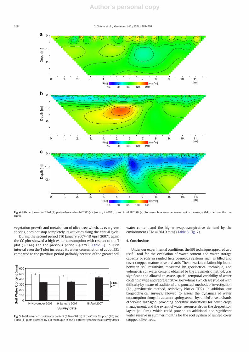
In Fig. 3a, b, c and 4a, b, c, the ERIs obtained from the geoelectricalmeasurements, performed in both CC and T plots in coincidence of thethree survey campaigns, are shown. Particularly, we reported thetomographies carried out in the row, at 0.4 m far from the tree trunk,because they showed the highest variability of soil ρ with respect tothe other ones. The ERIs reported ρ distribution along soil profiles11.5 m long and 3.0 m deep. Generally, the tomographies taken in theCC plot showed wide low resistivity areas, indicating water presencein the soil (Fig. 3a, b, c). These areas were particularly evident alongthe whole soil profile depicted by the tomography performed the 18April 2007 (Fig. 3c). Even the T plot showed at the same date low soil ρvalues limited to 0.0–1.5 m soil layer: under this depth the soil ρgradually reached the lowest values of the scale (Fig. 4c). Suchbehaviour could be also due to the canalization process of the injectedcurrent by thewet upper soil layers. On the other hand, in coincidenceof the first two measurement campaigns, the soil profiles of T plotshowed low-resistive areas as a result of a strong depletion of waterfrom the soil (Fig. 4a, b).

3.3. Assessment of the spatial and temporal variability of θv

The strong relation found between ρ and θv allowed to assess thespatial and temporal variability of θv in the soil of both the systemscompared, CC and T. Starting from the ρ values, obtained from thegeoelectrical measurements performed at the three survey cam-paigns, θv data were assessed by the exponential model (3) reportedin Fig. 2.

Total volumetric soil water content (soil layer: from 0.0 to 3.0 m),assessed in the CC and T plots at the 3 different survey dates, isreported in Fig. 5. The CC plot always had greater soil water contentthan the T one, which showed a significant water increase only incoincidence of the last survey carried out in April 2007.

The water content patterns along the soil profile at the threedifferent survey dates of both plots, CC and T, are shown in Fig. 6.

The initial soil water content, recorded in the two systems on 14November 2006, was substantially different being higher in the CC soilprofile compared to the T one: the former showed a greater watercontent below 0.6 m depth, while the latter kept soil water contentmore or less at the same level in the different soil layers. On 9 January2007, the CC soil showed no recharge of the first soil layers byprecipitation with respect to the first survey campaign. In addition, awater depletion occurred, especially between 0.6 m (limit depth forherbaceous roots) and 1.8 m depths. Such conditions were probablydue to the anomalous climatic pattern (low precipitation, high airtemperature) (Fig. 7) which led to a strong consumption of deepwater reserves by spontaneous vegetation and, especially, olive trees.Conversely, the T plot showed an increase of soil water content in thefirst soil layers (0.0–0.9 m). In coincidence of the last measurementcampaign (18 April 2007), both the compared systems showed asignificant increase of water content in the soil profile as a response tothe rainfall pattern recorded in the last experimental interval (10January–18 April 2007) (Table 3). Particularly, the CC plot was able torecover water reserve in the deepest soil layers exploited only by theolive root systems (Fig. 6). Instead, the T plot showed a continuousincrease of soil water content, especially in the shallow layers, neverreaching the water content of the CC plot (Fig. 6).

The differences found between CC and T plots could be explainedby the diverse capacity of the two systems to intercept and storerainwater. Furthermore, the water dynamics in the soil profile of theCC plot was strongly affected by crop transpiration.

The rainfall values recorded during the study period were thefollowing: 58.0 mm from 21 September 2006 to 14 November 2006;61.2 mm from 15 November 2006 till 9 January 2007; 211.4 mm from10 January 2007 to 18 April 2007. The 21 September was the starting

θve = 1.074 θvm - 0.022R = 0.911 p < 0.000

0.00

0.05

0.10

0.15

0.20

0.25

0.30

0.00 0.05 0.10 0.15 0.20 0.25 0.30

θvm (mm mm-1)

θve

(mm

mm

-1)

Fig. 1. Scatterplot of estimated vsmeasured volumetric water content values (θve vs θvm).

0.00

0.05

0.10

0.15

0.20

0.25

0.30

0 20 40 60 80 100 120 140

ρ (Ω.m)

θv (

mm

mm

-1)

Model: θv = β1 ρ β 2 θv = 1.641 ρ-0.599

R = 0.866 p < 0.000

Fig. 2. Relationship between resistivity (ρ, ohm m) and volumetric water content(θv, mm mm−1) for the examined soil from in-situ data (gravimetric method vs ERImeasurements).

166 G. Celano et al. / Geoderma 163 (2011) 163–170

Author's personal copy

date of the autumn–winter period, considered as the “rechargeperiod” of rainwater in the soil. Results showed that the CC systemwas more efficient than the T system to readily retain the rainwatereven when the amount of rainfall was very low as in the firstexamined period (Fig. 6). Higher macroporosity measured in the Ap1horizon of the CC soil with respect to the T one, allowed water toinfiltrate easily in the deepest layers (Palese et al., in press).Particularly, macroporosity in the CC plot was homogeneouslydistributed along the profile and mainly represented by elongatedtransmission pores (size class 50–500 μm), which are directlyinvolved in water fluxes within the soil (Pagliai and Vignozzi, 2002).In addition, the best permeability of CC soil could be also ascribed tothe presence of a dense net of roots belonging to the cover crops, ahigher organic matter content due to the medium-term adoption ofsustainable soil management practices, and an intense activity ofearthworms, noticed during the geoelectrical campaigns and the soilsamplings and also reported by other Authors (Beven and Germann,1982; Moreno et al., 1997). Also crop and pruning residues, retainedon the soil surface, increased water storage by minimising surfacesealing and directly reducing soil evaporation (Schwartz et al., 2010).

Conversely, the T plot showed a lesser ability to accept precipi-tation due to the presence of a compacted layer just below the tilled

soil which reduced the saturated hydraulic conductivity and hinderedvertical water infiltration Palese et al. (in press). Castro et al. (2006)reported a significant reduction in the field saturated hydraulicconductivity measured in tilled olive orchards. In addition, an increaseof water losses by soil evaporation was determined by the anomalousclimate recorded during the experimental period (Fig. 7) (Morin andBenyamini, 1977).

3.4. Water consumption estimation by the ERI technique

The knowledge of both soil water content, evaluated by means ofthe ERI technique, and precipitation pattern, allowed to estimate thewater consumption by each studied system, CC and T, using the soilwater balance approach (Eq. 2) (Table 3) (Fernández and Moreno,1999).

In the first survey period, from 14 November 2006 to 9 January2007, water consumption by the CC plot was about double comparedto the T plot (Table 3). Although the CC soil was able to store in thisperiod higher amounts of rainfall water (Fig. 5 and 6), it consumedmore water than T plot because of the transpiration of thespontaneous vegetation. As a matter of fact, in this period, theclimatic conditions were favorable (Fig. 7) for both spontaneous

a

b

c

0.

-1.

-2.Dep

th [m

]

0.

-1.

-2.Dep

th [m

]

0.

-1.

-2.Dep

th [m

]

0. 1. 2. 3. 4. 5. 6. 7. 8. 9. 10. 11.[m][Rho] [0hmxm]

5. 10. 20. 40. 80.

0. 1. 2. 3. 4. 5. 6. 7. 8. 9. 10. 11.[m][Rho] [0hmxm]

5. 10. 20. 40. 80.

0. 1. 2. 3. 4. 5. 6. 7. 8. 9. 10. 11.[m][Rho] [0hmxm]

5. 10. 20. 40. 80.

Fig. 3. ERIs performed in Cover Cropped (CC) plot on November 14 2006 (a), January 9 2007 (b), and April 18 2007 (c). Tomographies were performed out in the row, at 0.4 m farfrom the tree trunk.

167G. Celano et al. / Geoderma 163 (2011) 163–170

Author's personal copy

vegetation growth and metabolism of olive tree which, as evergreenspecies, does not stop completely its activities along the annual cycle.

During the second period (10 January 2007–18 April 2007), againthe CC plot showed a high water consumption with respect to the Tplot (+14%) and the previous period (+32%) (Table 3). In suchinterval even the T plot increased its water consumption of about 55%compared to the previous period probably because of the greater soil

water content and the higher evapotranspirative demand by theenvironment (ETo=204.9 mm) (Table 3, Fig. 7).

4. Conclusions

Under our experimental conditions, the ERI technique appeared as auseful tool for the evaluation of water content and water storagecapacity of soils in rainfed heterogeneous systems such as tilled andcover croppedmature olive orchards. The univariate relationship foundbetween soil resistivity, measured by geoelectrical technique, andvolumetric soil water content, obtained by the gravimetricmethod,wassignificant and allowed to assess spatial–temporal variability of watercontent inwide and representative soil volumeswhich are studiedwithdifficulty bymeans of traditional and punctualmethods of investigation(i.e., gravimetric method, resistivity blocks, TDR). In addition, ourbiogeophysical surveys, allowed to assess the dynamics of waterconsumption along the autumn–spring season by rainfed olive orchardsotherwise managed, providing operative indications for cover cropsmanagement, and the extent of water resource also in the deepest soillayers (N 1.0 m), which could provide an additional and significantwater reserve in summer months for the root system of rainfed covercropped olive trees.

a

b

c

0.

-1.

-2.Dep

th [m

]

0.

-1.

-2.Dep

th [m

]

0.

-1.

-2.Dep

th [m

]

0. 1. 2. 3. 4. 5. 6. 7. 8. 9. 10. 11.[m][Rho] [0hmxm]

15. 30. 60. 120. 240.

15. 30. 60. 120. 240.

15. 30. 60. 120. 240.

0. 1. 2. 3. 4. 5. 6. 7. 8. 9. 10. 11.[m][Rho] [0hmxm]

0. 1. 2. 3. 4. 5. 6. 7. 8. 9. 10. 11.[m][Rho] [0hmxm]

Fig. 4. ERIs performed in Tilled (T) plot on November 14 2006 (a), January 9 2007 (b), and April 18 2007 (c). Tomographies were performed out in the row, at 0.4 m far from the treetrunk.

0

100

200

300

400

500

600

14 November 2006 9 January 2007 18 April2007

Survey date

So

il W

ater

Co

nte

nt

(mm

)

CCT

Fig. 5. Total volumetric soil water content (0.0 m–3.0 m) of the Cover Cropped (CC) andTilled (T) plots assessed by ERI technique in the 3 different geoelectrical survey dates.

168 G. Celano et al. / Geoderma 163 (2011) 163–170

Author's personal copy

Acknowledgements

This research was financed by the Italian Ministry of Agricultureand Forestry (RIOM Project “Ricerca ed Innovazione per l'OlivicolturaMeridionale”). The authors thank the Editor and the Reviewers fortheir precious suggestions and Mr. Angelo Mossuto (Natura Informa-tica Società Cooperativa Sociale) for his valuable support in samplingand experimental field management.

References

Amato, M., Basso, B., Celano, G., Bitella, G., Morelli, G., Rossi, R., 2008. In-situ detection oftree-root distribution and biomass with multi-electrode resistivity imaging. TreePhysiology 28, 1441–1448.

Besson, A., Cousin, I., Bourennane, H., Nicoullaud, B., Pasquier, C., Richard, G., Dorigny,A., King, D., 2010. The spatial and temporal organization of soil water at the fieldscale as described by electrical resistivity measurements. European Journal of SoilScience 61, 120–132.

Beven, K., Germann, P., 1982. Macropores and water flow in soils. Water ResourcesResearch 18, 1325–1331.

Binley, A., Cassiani, G., Middelton, R., Winship, P., 2002. Vadose zone flow modelparameterisation using cross-borehole radar and resistivity imaging. Journal ofHydrology 267, 147–159.

Böhm, W., 1979. Methods of studying root systems. Ecological Studies 33. Springer-Verlag, Berlin.

Castro, G., Romero, R., Gómez, J.A., Fereres, E., 2006. Rainfall redistribution beneath anolive orchard. Agricultural Water Management 86, 249–258.

Celano, G., Palese, A.M., Martorella, E., Tuzio, A.C., Zuardi, D., Lazzari, L., Xiloyannis, C.,2010. Geo-electrical survey on the soil of an apricot orchard grown under semi-aridconditions. Acta Horticulturae 862, 425–428.

Fernández, J.E., Moreno, F., 1999.Water use by the olive tree. Journal of Crop Production2, 101–162.

Fukue, M., Minatoa, T., Horibe, H., Taya, N., 1999. The microstructure of clay given byresistivity measurements. Engineering Geology 54, 43–53.

Gardner, W.H., 1986. Water Content, In: Klute, A. (Ed.), Methods of Soil Analysis, Part 1,Second Edn. Am. Soc. Agron. Publ, Madison, WI, pp. 493–544.

Hagrey, S.A. al, 2007. Geophysical imaging of root-zone, trunk, and moistureheterogeneity. Journal of Experimental Botany 58 (4), 839–854.

Hagrey, S.A. al, Meissner, R., Werban, U., Ismaeil, A., Rabbel, W., 2004. Hydro-, Bio-Geophysics. The Leading Edge 23, 670–674.

Hagrey, S.A. al, Michaelsen, J., 2002. Hydrogeophysical soil study at a drip irrigatedorchard, Portugal. European Journal of Environment and Engineering Geophysics 7,75–93.

Kachanoski, R.G., de Jong, E., Hendrickx, J.M.H., 2002. Nonintrusive water contentmeasurement in the field. Section 3.1.3.2. In: Dane, J.H., Topp, G.C. (Eds.), Methods

0

1

2

3

4

5

6

7

8

Soil layer (m)

14 November 2006 18 April 2007

So

il W

ater

Co

nte

nt

(mm

)

T

0

1

2

3

4

5

6

7

8

0.0-0.3 0.3-0.6 0.6- 0.9 0.9-1.2 1.2-1.5 1.5-1.8 1.8-2.1 2.1- 2.4 2.4-2.7 2.7-3.0

0.0-0.3 0.3-0.6 0.6- 0.9 0.9-1.2 1.2-1.5 1.5-1.8 1.8-2.1 2.1- 2.4 2.4-2.7 2.7-3.0

Soil layer (m)

So

il W

ater

Co

nte

nt

(mm

) 14 November 2006 9 January 2007

9 January 2007

18 April 2007CC

Fig. 6. Soil water content (mm) at the different soil depths of Cover Cropped (CC) and Tilled (T) plots evaluated by ERI technique (soil layer: 0.0–3.0 m).

0

5

10

15

20

25

30

10/9/06 10/10/06 9/11/06 9/12/06 8/1/07 7/2/07 9/3/07 8/4/07 8/5/07

date

T °

C

mean T min Tmax T

Fig. 7. Daily mean, min and max air temperatures recorded at the experimental sitefrom September 21 2006 till April 18 2007.

Table 3Estimation of water consumption according to the simplified equation of water balance(ETc=R−Δθv) in the Cover Cropped (CC) and Tilled (T) plots using ERI technique (soillayer: 0.0–3.0 m). ETo=reference evapotranspiration; R=rainfall; Δθv=differencebetween the water stored in the soil in the lapse of time considered.

14 November 06–9January 07

10 January 07–18April 07

14 November06–18 April 07

mm mm d−1 mm mm d−1 mm mm d−1

ETo 64.8 1.14 204.9 2.07 269.7 1.73Δθv(CC) −43.7 −0.77 57.3 0.58 13.6 0.09Δθv (T) 2.4 0.02 79.4 0.80 81.8 0.52R 61.2 1.07 211.4 2.14 272.6 1.75

ETc ETc ETc

mm mm d−1 mm mm d−1 mm mm d−1

CC 104.9 1.84 154.1 1.56 259.4 1.66T 58.8 1.03 132 1.33 190.2 1.23CC-T 46.1 0.81 22.1 0.22 68.2 0.44

169G. Celano et al. / Geoderma 163 (2011) 163–170

Author's personal copy

of soil analysis. Part 4. Physical Methods. Soil Science Society of America, Madison,Wisconsin, pp. 497–501.

LaBrecque,D.J.,Miletto,M.,Daily,W.D., Ramirez,A.L.,Owen, E., 1996. Theeffects of noise onOccam's inversion of resistivity tomography data. Geophysics 61, 538–548.

Lazzari, L., 2008. Study of spatial variability of soil root zone properties using electricalresistivity technique. PhD thesis. Università degli Studi della Basilicata, pp 107.

Loperte, A., Satriani, A., Lazzari, L., Amato, M., Celano, G., Lapenna, V., Morelli, G., 2006. 2Dand 3D high resolution geoelectrical tomography for non-destructive determinationof the spatial variability of plant root distribution: Laboratory experiments and fieldmeasurements. Geophysical Research Abstracts, 8. Wien, p. 06749.

McCarter, W.J., 1984. The electrical resistivity characteristics of compacted clays.Geotechnique 34, 263–267.

Michot, D., Dorigny, A., Benderitter, Y., 2000. Mise en evidence par resistivité electriquedes ecoulements préférentiels et de l'assèchement par le maıs d'un calcisol deBeauce irrigué. C.R. Acad. Sci. 332, 29–36.

Montoroi, J.P., Bellier, G., Larvy Delarivière, J., 1999. Détermination de la relationrésistivité électrique – teneur en eau au laboratoire. Application aux sols de Tunisiecentrale. Colloque GEOFCAN Géophysique des sols et des formations superficielles,11–12 Sseptembre 1997, Bondy, France, pp. 153–159.

Morelli, G., LaBrecque, D.J., 1996. Advances in ERT inverse modeling. European Journalof Environmental and Engineering Geophysics 1, 171–186.

Moreno, F., Pelegrín, F., Fernández, J.E., Murillo, J.M., 1997. Soil physical properties,water depletion and crop development under traditional and conservation tillagein southern Spain. Soil & Tillage Research 41, 25–42.

Morin, J., Benyamini, Y., 1977. Rainfall infiltration into bare soils. Water ResourcesResearch 5, 813–817.

Pagliai, M., Vignozzi, N., 2002. The soil pore system as an indicator of soil quality.Advances in GeoEcology 35, 71–82.

Palese, A.M., Agnelli, A.E., Celano, G., Platinetti, M., Vignozzi, N., Xiloyannis, C., in press.Soil management and soil water balance in a mature rainfed olive orchard.Proceedings Olivebioteq 2009 – Sfax (Tunisia), December 15–19, 2009.

Rhoades, J.D., 1982. Soluble salts. In: Page, A.L., Miller, H., Keeney, D.R. (Eds.), Methodsof soil analysis, Part 2. Chemical andmicrobiological properties. Soil Science Societyof American, Inc., Madison, WI, pp. 167–179.

Ribolini, A., Guglielmin, M., Fabre, D., Bodin, X., Marchisio, M., Sartini, S., Spagnolo, M.,Schoeneich, P., 2010. The internal structure of rock glaciers and recentlydeglaciated slopes as revealed by geoelectrical tomography: insights on permafrostand recent glacial evolution in the Central and Western Alps (Italy–France).Quaternary Science Reviews 29 (3-4), 507–521.

Samouëlian, A., Cousin, I., Tabbagh, A., Bruand, A., Richard, G., 2005. Electrical resistivitysurvey in soil science: a review. Soil & Tillage Research 83, 173–193.

Schwartz, R.C., Baumhardt, R.L., Evett, S.R., 2010. Tillage effects on soilwater redistributionand bare soil evaporation throughout a season. Soil & Tillage 110, 221–229.

Srayeddin, I., Doussan, C., 2009. Estimation of the spatial variability of root water uptakeof maize and sorghum at the field scale by electrical resistivity tomography. Plantand Soil 319, 185–207.

Tabbagh, A., Dabas, M., Hesse, A., Panissod, C., 2000. Soil resistivity: a non-invasive toolto map soil structure horizonation. Geoderma 97, 393–404.

Zhou, Q.Y., Shimada, J., Sato, A., 2001. Three-dimensional spatial and temoralmonitoring of soil water content using electrical resitivity tomography. WaterResources Research 37, 273–285.

170 G. Celano et al. / Geoderma 163 (2011) 163–170