Florida State University Libraries

Electronic Theses, Treatises and Dissertations The Graduate School

2010

Evaluation of Dynamic Load AllowanceFactors for Reinforced Concrete HighwayBridgesSharnie Fiona Earle

Follow this and additional works at the FSU Digital Library. For more information, please contact lib-ir@fsu.edu

THE FLORIDA STATE UNIVERSITY

FAMU-FSU COLLEGE OF ENGINEERING

EVALUATION OF DYNAMIC LOAD ALLOWANCE FACTORS FOR REINFORCED

CONCRETE HIGHWAY BRIDGES

By

SHARNIE EARLE

A Thesis submitted to the

Department of Civil and Environmental Engineering

in partial fulfillment of the

requirements for the degree of

Master of Science

Degree Awarded:

Spring Semester, 2010

The members of the committee approve the thesis of Sharnie Earle defended on April 4, 2010.

____________________________________

Jerry Wekezer

Professor Directing Thesis

____________________________________

Michelle Rambo-Roddenberry

Committee Member

____________________________________

Primus Mtenga

Committee Member

Approved:

______________________________________________________________

Kamal Tawfiq, Chair, Department of Civil and Environmental Engineering

______________________________________________________________

Chen, Dean, FAMU-FSU College of Engineering

The Graduate School has verified and approved the above-named committee members.

ii  

I dedicate this to my mother, Auleen Earle and to my father Lexley Earle. Without the support

of my mother I would not have been able to attend Florida State University. She supported me

financially and emotionally. Without her help, none of this would be possible. My father

provided me with the technical guidance that I needed in order to become a successful Civil

Engineer. I would also like to thank Mark Coppola Jr., who encouraged me all throughout

engineering school. Whenever I thought I could not do it, he would always reassure me that I

was too smart to give up. Lastly, to all my extended family, who over the years realized the

passion that I had for school and they too, began supporting me.

iii  

ACKNOWLEDGEMENTS I would like to acknowledge Professor Jerry Wekezer at the FAMU-FSU College of Engineering for all of his guidance throughout my Master of Science research. His knowledge and assistants was of the utmost importance when putting this research together. I would also like to acknowledge Mr. Marc Ansley for his technical support throughout the research. A special thanks goes to Piotr Szurgott, Hongyi Li, and Dr. Kwasniewski for their outstanding work on previous research projects which, opened the door for my research.

iv  

TABLE OF CONTENTS

List of Tables . . . . . . . . . . . . . . . . . . . . . . . . . . . . . . . . . . . . . . . . . . . . . . . . . . . . . . . . . . . . . . vi List of Figures . . . . . . . . . . . . . . . . . . . . . . . . . . . . . . . . . . . . . . . . . . . . . . . . . . . . . . . . . . . . . . viii

Abstract . . . . . . . . . . . . . . . . . . . . . . . . . . . . . . . . . . . . . . . . . . . . . . . . . . . . . . . . . . . . . . x

1. INTRODUCTION . . . . . . . . . . . . . . . . . . . . . . . . . . . . . . . . . . . . . . . . . . . . . . . . . . . . . . . . 1 1.1 Problem Statement . . . . . . . . . . . . . . . . . . . . . . . . . . . . . . . . . . . . . . . . . . . . . . . . . . 1 1.2 Research Objective . . . . . . . . . . . . . . . . . . . . . . . . . . . . . . . . . . . . . . . . . . . . . . . . . . 3 1.3 Significance of Research . . . . . . . . . . . . . . . . . . . . . . . . . . . . . . . . . . . . . . . . . . . . 4

2. LITERATURE REVIEW . . . . . . . . . . . . . . . . . . . . . . . . . . . . . . . . . . . . . . . . . . . . . . . . . . 6 2.1 Bridge Dynamic Effect in AASHTO Specification . . . . . . . . . . . . . . . . . . . . . . . . . . 6 2.2 FE Modeling of Highway Bridge . . . . . . . . . . . . . . . . . . . . . . . . . . . . . . . . . . . . . . 7 2.3 Analysis of Elastomeric Bearing Pads . . . . . . . . . . . . . . . . . . . . . . . . . . . . . . . . 10 2.4 Validation and Verification of FE Model . . . . . . . . . . . . . . . . . . . . . . . . . . . . . . . . 13 2.5 FE Modeling of Vehicles . . . . . . . . . . . . . . . . . . . . . . . . . . . . . . . . . . . . . . . . . . . . 14

3. SELECTION OF OBJECTS FOR TESTING . . . . . . . . . . . . . . . . . . . . . . . . . . . . . . . . 18 3.1 Use of Existing Vehicle Models . . . . . . . . . . . . . . . . . . . . . . . . . . . . . . . . . . . . . . 18 3.2 Selection of Highway Bridge . . . . . . . . . . . . . . . . . . . . . . . . . . . . . . . . . . . . . . . . . . . . 21

4. DEVELOPMENT OF THE FINITE ELEMENT MODEL . . . . . . . . . . . . . . . . . . . . 22 4.1 Geometric Adjustment of Existing FE Model . . . . . . . . . . . . . . . . . . . . . . . . . . 23 4.2 Material Characterization . . . . . . . . . . . . . . . . . . . . . . . . . . . . . . . . . . . . . . . . . . . 32 4.3 Importing of Key File . . . . . . . . . . . . . . . . . . . . . . . . . . . . . . . . . . . . . . . . . . . . . . . . . . 35

5. ELASTOMERIC BEARING PADS . . . . . . . . . . . . . . . . . . . . . . . . . . . . . . . . . . . . . . 41

5.1 Improvements of Bearing Pad Design . . . . . . . . . . . . . . . . . . . . . . . . . . . . . . . . 45 5.2 Analysis of Bearing Pad Improvements . . . . . . . . . . . . . . . . . . . . . . . . . . . . . . . . 52 5.3 Parametric Study of Reinforced Neoprene Bearing Pads . . . . . . . . . . . . . . . . . . . . 55

6. VERIFICATION AND VALIDATION OF NEOPRENE BEARING PADS . . . . . . . . 67 6.1 Verification and Validation of Existing FE Model . . . . . . . . . . . . . . . . . . . . . . . . . . 68

7. DYNAMIC LOAD ALLOWANCE FACTORS . . . . . . . . . . . . . . . . . . . . . . . . . . . . . . . . 72 7.1 Evaluation of Dynamic Load Allowance . . . . . . . . . . . . . . . . . . . . . . . . . . . . . . . . 73 7.2 Summary and Conclusion . . . . . . . . . . . . . . . . . . . . . . . . . . . . . . . . . . . . . . . . . . . . 78 7.3 Future Work . . . . . . . . . . . . . . . . . . . . . . . . . . . . . . . . . . . . . . . . . . . . . . . . . . . . . . . . 79 7.4 Bibliography Sketch . . . . . . . . . . . . . . . . . . . . . . . . . . . . . . . . . . . . . . . . . . . . . . . . . . 82

v  

LIST OF TABLES

4.1 Units adopted for FE analysis in this study . . . . . . . . . . . . . . . . . . . . . . . . . . . . . . . . . 24 4.2 Summary of concrete slab parameters . . . . . . . . . . . . . . . . . . . . . . . . . . . . . . . . . . . . . . . 26 4.3 Material properties for concrete beams . . . . . . . . . . . . . . . . . . . . . . . . . . . . . . . . . . . . . . . 26 4.4 Dimensions for ASTM standard reinforcing bars used in bridge structure . . . . . . . . 33 4.5 Material properties of the concrete slab . . . . . . . . . . . . . . . . . . . . . . . . . . . . . . . . . . . . . . . 34 4.6 Material properties for concrete girders . . . . . . . . . . . . . . . . . . . . . . . . . . . . . . . . . . . . . . . 35 4.7 Summary information for No Name Creek FE Model . . . . . . . . . . . . . . . . . . . . . . . . . . . 40 5.1 FDOT bearing pad dimensions for AASHTO beams . . . . . . . . . . . . . . . . . . . . . . . . . . . 45 5.2 Typical bearing properties . . . . . . . . . . . . . . . . . . . . . . . . . . . . . . . . . . . . . . . . . . . . . 47 5.3 Dimension tolerance for bearing pads . . . . . . . . . . . . . . . . . . . . . . . . . . . . . . . . . . . . . . . 49 5.4 Result of geometric design . . . . . . . . . . . . . . . . . . . . . . . . . . . . . . . . . . . . . . . . . . . . . 51 5.5 Summary of FE Model for Shear Test . . . . . . . . . . . . . . . . . . . . . . . . . . . . . . . . . . . . . . . 57 5.6 Material Properties for Compression Test . . . . . . . . . . . . . . . . . . . . . . . . . . . . . . . . . 61 6.1 Comparison metrics for analytical curves . . . . . . . . . . . . . . . . . . . . . . . . . . . . . . . . . 68 7.1 Total displacement values for each case . . . . . . . . . . . . . . . . . . . . . . . . . . . . . . . . . . . . . . 71 7.2 Complete displacement values . . . . . . . . . . . . . . . . . . . . . . . . . . . . . . . . . . . . . . . . . . . . 73 7.3 Results for displacement Dynamic Load Allowance . . . . . . . . . . . . . . . . . . . . . . . . . . 73 7.4 Dynamic Load Allowance result for strains . . . . . . . . . . . . . . . . . . . . . . . . . . . . . . . . 74 7.5 Final results for improvement of neoprene pads . . . . . . . . . . . . . . . . . . . . . . . . . . . . . . . . 75 7.6 Results for new bridge model with improved pads . . . . . . . . . . . . . . . . . . . . . . . . . . 75

vi  

LIST OF FIGURES

2.1 Dynamic analysis procedure of vehicle and bridge interaction . . . . . . . . . . . . . . . . . . . . 8 2.2 Grillage model . . . . . . . . . . . . . . . . . . . . . . . . . . . . . . . . . . . . . . . . . . . . . . . . . . . . . . . . 9 2.3 Finite element model of a bridge (Tedesco, Stallings, & El-Mihimy, 1999) . . . . . . . . 10 2.4 Bearing deformation due to compression . . . . . . . . . . . . . . . . . . . . . . . . . . . . . . . . 11 2.5 Bearing deformation due to shear . . . . . . . . . . . . . . . . . . . . . . . . . . . . . . . . . . . . . . 11 2.6 Bearing deformation due to rotation . . . . . . . . . . . . . . . . . . . . . . . . . . . . . . . . . . . . . . 11 2.7 Shape factor dimensions for neoprene pads . . . . . . . . . . . . . . . . . . . . . . . . . . . . . . . . 12 2.8 Types of neoprene pads . . . . . . . . . . . . . . . . . . . . . . . . . . . . . . . . . . . . . . . . . . . . . . . . . . 13 2.9 Simplified analytical vehicle models . . . . . . . . . . . . . . . . . . . . . . . . . . . . . . . . . . . . . . 15 2.10 Three dimensional analytical vehicle model . . . . . . . . . . . . . . . . . . . . . . . . . . . . . . . . 15 2.11 Analytical model of an AASHTO HS20-44 truck . . . . . . . . . . . . . . . . . . . . . . . . . . 16 2.12 Finite element models available in public domain . . . . . . . . . . . . . . . . . . . . . . . . . . 17 2.13 FE model of the tractor-trailer and lowboy . . . . . . . . . . . . . . . . . . . . . . . . . . . . . . . . 17 3.1 Detailed sketch of a Mack CH613 Tractor-Trailer truck . . . . . . . . . . . . . . . . . . . . . . . . . . 19 3.2 Mack CH613 Tractor-Trailer truck . . . . . . . . . . . . . . . . . . . . . . . . . . . . . . . . . . . . . . 19 3.3 Bridge #540074 used for FE modeling . . . . . . . . . . . . . . . . . . . . . . . . . . . . . . . . . . . . . . 20 3.4 Localization of the bridge used for modeling . . . . . . . . . . . . . . . . . . . . . . . . . . . . . . . 21 4.1 FE model of concrete slab with LS-Dyna summary . . . . . . . . . . . . . . . . . . . . . . . . . . 25 4.2 AASHTO dimensions . . . . . . . . . . . . . . . . . . . . . . . . . . . . . . . . . . . . . . . . . . . . . . . . . . 27 4.3 Girder modification in z-direction . . . . . . . . . . . . . . . . . . . . . . . . . . . . . . . . . . . . . . 28 4.4 FE model of completed girder modifications . . . . . . . . . . . . . . . . . . . . . . . . . . . . . . . . 29

vii  

4.5 FE model of traffic barriers railings . . . . . . . . . . . . . . . . . . . . . . . . . . . . . . . . . . . . . . 31 4.6 FE model of diaphragms . . . . . . . . . . . . . . . . . . . . . . . . . . . . . . . . . . . . . . . . . . . . . . . . . . 32 4.7 FE model of neoprene pads . . . . . . . . . . . . . . . . . . . . . . . . . . . . . . . . . . . . . . . . . . . . 33 4.8 Cross-section of traffic railing barriers . . . . . . . . . . . . . . . . . . . . . . . . . . . . . . . . . . . . . . 34 4.9 FE model of reinforcements . . . . . . . . . . . . . . . . . . . . . . . . . . . . . . . . . . . . . . . . . . . . 35 4.10 *Part interface dialog box for LS-Dyna . . . . . . . . . . . . . . . . . . . . . . . . . . . . . . . . . . . . . . 37 4.11 LS-Dyna error reports . . . . . . . . . . . . . . . . . . . . . . . . . . . . . . . . . . . . . . . . . . . . . . . . . . 40 4.12 Complete FE model of new bridge, No Name Creek . . . . . . . . . . . . . . . . . . . . . . . . . . 40 5.1 Time histories of existing material pad parameters . . . . . . . . . . . . . . . . . . . . . . . . . . 41 5.2 Detailed sketch of elastomeric bearing pad cross-section . . . . . . . . . . . . . . . . . . . . 46 5.3 Original neoprene pad used on existing FE bridge model . . . . . . . . . . . . . . . . . . . . 48 5.4 Improved neoprene pad for existing FE model; a) top pad, b) bottom pad . . . . . . . . 48 5.5 Graph of shape factor vs. internal layer thickness . . . . . . . . . . . . . . . . . . . . . . . . . . 50 5.6 Graph of geometric study . . . . . . . . . . . . . . . . . . . . . . . . . . . . . . . . . . . . . . . . . . . . . . . . . . 52 5.7 In-Lab Shear-Test Apparatus . . . . . . . . . . . . . . . . . . . . . . . . . . . . . . . . . . . . . . . . . . . . 56 5.8 Detailed Sketch of Shear-Test Apparatus . . . . . . . . . . . . . . . . . . . . . . . . . . . . . . . . 57 5.9 FE Model of Shear Test . . . . . . . . . . . . . . . . . . . . . . . . . . . . . . . . . . . . . . . . . . . . . . . . . . 59 5.10 Results for Case 1 compression test; a) displacement, b) strain . . . . . . . . . . . . . . 60 5.11 Results for Case 2 compression test; a) displacement, b) strain . . . . . . . . . . . . . . 60 5.12 Results for Case 3 compression test; a) displacement, b) strain . . . . . . . . . . . . . . 61 5.13 Load vs Displacement . . . . . . . . . . . . . . . . . . . . . . . . . . . . . . . . . . . . . . . . . . . . . . . . . . 63 5.14 Displacement vs Time . . . . . . . . . . . . . . . . . . . . . . . . . . . . . . . . . . . . . . . . . . . . . . . . . . 63 5.15 Stress vs Time . . . . . . . . . . . . . . . . . . . . . . . . . . . . . . . . . . . . . . . . . . . . . . . . . . . . . . . . 64

viii  

5.16 Strain vs Displacement . . . . . . . . . . . . . . . . . . . . . . . . . . . . . . . . . . . . . . . . . . . . . . . . . . 64 5.17 Stress vs Strain . . . . . . . . . . . . . . . . . . . . . . . . . . . . . . . . . . . . . . . . . . . . . . . . . . . . . . . . 65 6.1 Dynamic test of vehicle-bridge interaction, (a) Full-scale field test and (b) Finite Element simulation . . . . . . . . . . . . . . . . . . . . . . . . . . . . . . . . . . . . . . . . . . . . . . . . . . 67 6.2 Case 1 strain results . . . . . . . . . . . . . . . . . . . . . . . . . . . . . . . . . . . . . . . . . . . . . . . . . . 69 6.3 Case 2 strain results . . . . . . . . . . . . . . . . . . . . . . . . . . . . . . . . . . . . . . . . . . . . . . . . . . 69 6.4 Case 3 strain results . . . . . . . . . . . . . . . . . . . . . . . . . . . . . . . . . . . . . . . . . . . . . . . . . . 70

ix  

x  

ABSTRACT

The evaluation of existing structures is critical for the efficient management of transportation

facilities, especially bridges. According to the Florida Department of Transportation Plan,

Safety, and System Management, which include bridge repairs and replacements, a cost of about

30% of all state and federal revenues will be needed in order to get the nation’s bridge integrity

to a sufficient level [4]. ASCE estimates $930 billion dollars will be needed within 5 years in

order to improve all roads and bridges. This project responds to the growing need to rehabilitate

our nation’s bridges by focusing on vehicle-bridge interaction. Frequently, bridges are evaluated

using traditional stability methods and simplified static analysis methods.

The main objective of this research was the analysis of an already verified and validated bridge

model in order to improve on the dynamic nature of vehicle-bridge interaction. Special attention

was made to the improvement of the elastomeric bearing pads in the existing model. The main

focus of the research was placed on this part of the bridge due to the fact that these pads are ideal

for bridge design because they are economical, effective, and require no maintenance. They

deflect in shear to accommodate expansion, contraction, and end rotation of the bridge. There is

no need for lubrication, cleaning, nor do they have the opportunity to seize. In order to analyze

the improvements of the older bearing pads, an in-lab compression test was created using the

same finite element software that was used to create the bridge model. Several compression tests

were performed using different material properties in order to determine which set of material

characteristics would yield the best results for the improvement of these pads. Once these

parameters were determined, they were then verified and validated by a program known as the

Roadside Safety Validation and Verification Program, RSVVP. This program is an essential part

when developing a model if the model is to be accepted and used to support decision making.

The parameters that yield the closest results to the actual field test were then implemented onto

the new bridge model. This ensured that the new bridge model was in fact a better representation

of what happens in the field. A final calculation of the dynamic load allowance, DLA verified

that the vehicle-bridge interaction was successful due to the DLA factor decreasing when

compared to the previous calculated DLA factors from an existing vehicle-bridge interaction

research.

CHAPTER 1

INTRODUCTION

This project responds to the growing need to rehabilitate our nation’s roads, highways, and

bridges. With the recent report card from the American Society of Civil Engineers giving

America’s roadways and bridges a grade of D, it is vital more than ever to reduce the

deterioration of our country’s infrastructure. According to ASCE, an estimated $930 billion

dollars within 5 years will be needed to improve our nation’s roadways and bridges [1]. A price

tag like this can be reduced significantly if the proper operation and maintenance are performed.

In order to reduce this problem, knowledge of the actual load effects and structure resistance is

necessary. This information will be very useful for determining the load carrying capacity and

the condition of structures. It can also help in making management decisions, such as

establishing permissible weight limits for certain roadways and bridges and most importantly

provide fundamental economic and safety implications. Advanced structural analysis and

evaluation procedures can also be applied to a structure that exhibits behavior difficult to explain

such as, excessive vibration, deflection, and others.

Frequently, bridges are evaluated using simplified static analysis methods. Unfortunately, these

methods do not represent what is actually happening in the structure, due to the ignorance of

certain dynamic effects. The dynamic nature of live loads and vehicle-bridge interaction is not

sufficiently considered in the design process. Dynamic Load Allowance suggested by the

current bridge design codes usually lead to conservative solutions, especially for overloaded

vehicles. Accurate and inexpensive methods are needed for diagnostics and verification of the

actual dynamic effect on our nation’s bridges and the impact factor associated with them.

Traditional bridge analysis is based on several simplifications of geometry, material, boundary

conditions and loading. Bridge live load is considered one of the most questionable

simplifications. The interaction between a vehicle and the bridge structure is usually represented

by concentrated and uniformly distributed static loads. Dynamic effects of the actual live load

are considered by scaling up the static loads by values known as impact factors. The magnitude

of the dynamic load allowance, DLA is usually determined based on the simplifications and was

1  

related only to the length of the bridge. Unfortunately, the bridge’s surface roughness and the

dynamic characteristics of the vehicle were ignored.

Due to the increasing computational capabilities of computers and the development of

commercial finite element programs, advanced numerical and 3-D dynamic analysis of bridge

structures are calculated faster and easier than ever before. Growing knowledge of finite element

analysis is making it possible to create more detailed 3-D models of bridges that contain a large

amount of finite elements with consistent mass and stiffness distributions. Commercial finite

element software has also allowed for advanced material models of steel and concrete, options

for modeling rebar for reinforcement, application of different types of constraints, and damping

options which allows for more accurate description of the actual bridge behavior. There are also

finite element models of vehicles available in the public domain. These models are ready to use

but may have different levels of detailed representation for the suspension system, kinematical

characteristics of the vehicle components and wheel models. Once improvements have been

made, these models can be used successfully for simulation of truck passes onto the bridge

structure. Applications of these models will allow for more complex mechanical phenomena,

such as contact between wheels and pavement surface, impact forces caused by surface

discontinuities, and time dependence of moving live loads caused by dynamic interaction among

suspended masses representing vehicle components. Actual live loads caused by overloaded

heavy vehicles can also be modeled.

A full scale bridge test should be carried out in order to validate computational dynamic analysis.

Validated finite element models can provide extensive information about the structural behavior,

which is both expensive and difficult, if not impossible, to obtain through experimental study

only. This project focuses on dynamic load allowance factors for short and medium span

reinforced concrete bridges, involving advanced finite element analysis and field testing.

2  

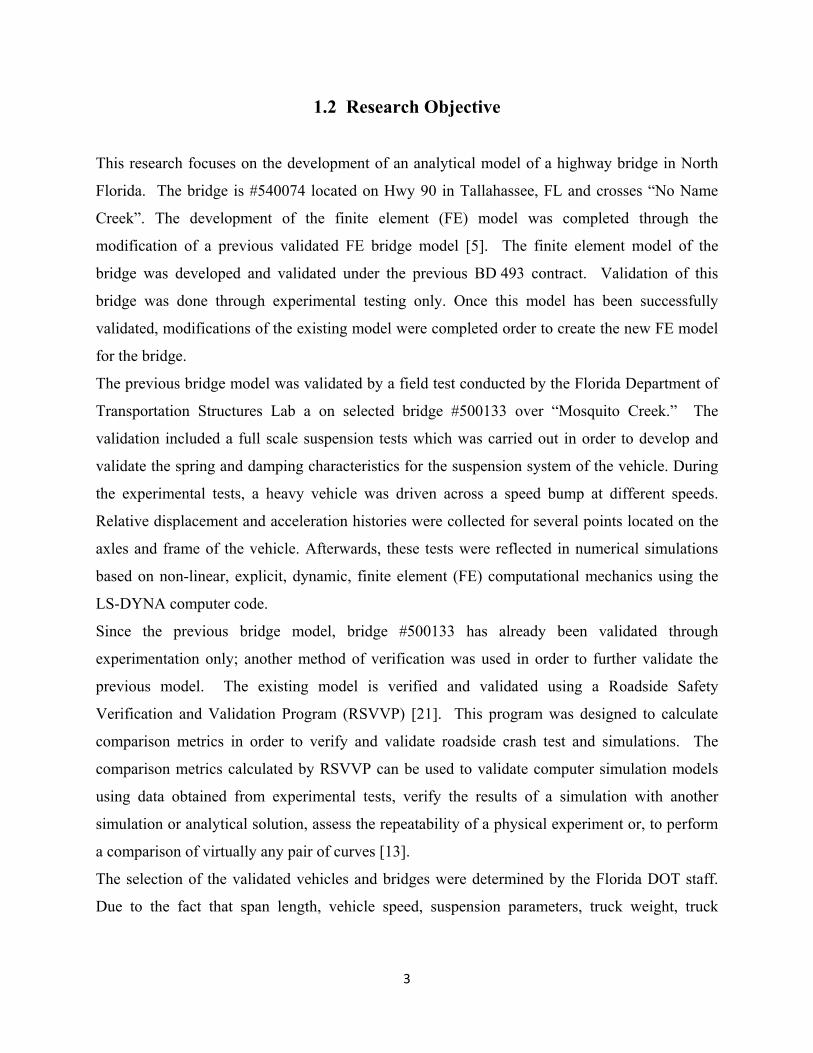
1.2 Research Objective

This research focuses on the development of an analytical model of a highway bridge in North

Florida. The bridge is #540074 located on Hwy 90 in Tallahassee, FL and crosses “No Name

Creek”. The development of the finite element (FE) model was completed through the

modification of a previous validated FE bridge model [5]. The finite element model of the

bridge was developed and validated under the previous BD 493 contract. Validation of this

bridge was done through experimental testing only. Once this model has been successfully

validated, modifications of the existing model were completed order to create the new FE model

for the bridge.

The previous bridge model was validated by a field test conducted by the Florida Department of

Transportation Structures Lab a on selected bridge #500133 over “Mosquito Creek.” The

validation included a full scale suspension tests which was carried out in order to develop and

validate the spring and damping characteristics for the suspension system of the vehicle. During

the experimental tests, a heavy vehicle was driven across a speed bump at different speeds.

Relative displacement and acceleration histories were collected for several points located on the

axles and frame of the vehicle. Afterwards, these tests were reflected in numerical simulations

based on non-linear, explicit, dynamic, finite element (FE) computational mechanics using the

LS-DYNA computer code.

Since the previous bridge model, bridge #500133 has already been validated through

experimentation only; another method of verification was used in order to further validate the

previous model. The existing model is verified and validated using a Roadside Safety

Verification and Validation Program (RSVVP) [21]. This program was designed to calculate

comparison metrics in order to verify and validate roadside crash test and simulations. The

comparison metrics calculated by RSVVP can be used to validate computer simulation models

using data obtained from experimental tests, verify the results of a simulation with another

simulation or analytical solution, assess the repeatability of a physical experiment or, to perform

a comparison of virtually any pair of curves [13].

The selection of the validated vehicles and bridges were determined by the Florida DOT staff.

Due to the fact that span length, vehicle speed, suspension parameters, truck weight, truck

3  

position on bridge lane, and road surface condition have a significant influence on dynamic

responses, emphasis were placed on these specific parameters.

The main focus of the new FE model will be the enhancement of the elastomeric neoprene

bearing pads, application of the Roadside Safety Verification and Validation Program, and the

evaluation of Dynamic Load Allowance. Since these pads have a proven long and successful

record of performance supporting bridges, railroads, buildings, and heavy machinery, they will

be a key factor in the improvement of the FE model, bridge #540074. These improvements will

allow for a better correlation between the experimental test and the numerical simulation.

A finite element model of an in-lab shear test was also developed using Hypermesh. This model

was used solely for the investigation of the neoprene bearing pads. In order to perform

successful parametric study different material characteristics were investigated and the results of

the compression test will give us a good idea of which parameters were the most suitable for the

chosen bearing pad design. Once these parameters were determined, they were then

implemented onto the new bridge model.

Parameters such as shape factor, shear modulus, Poisson ratio, bulk modulus were the focus of

improving the bearing pads. Once improvements have been made, a Roadside Verification and

Validation Program were used in order to analyze the result of the existing model with the new

neoprene bearing pad parameters. This is a vital part in the research because it showed the

improvement of the numerical results, when compared to the experimental results. Whichever

neoprene pad parameter yields the closest result to the actual field test, those parameters were

used when modeling the new FE model, bridge #540074 “No Name Creek”. By modifying the

new FE model with the existing bridge model results, it helped in verifying the new model

without any experimental test.

1.3 Significance of Research

The U.S. Department of Transportation has seen deterioration in the nations bridges for years.

With roughly 12% of our National Bridge Inventory classified as structurally deficient, research

in this area has become increasingly in demand, especially in the state of Florida. The Florida

Department of Transportation faces a challenge of allowing larger and heavier vehicles on

Florida’s highway and bridges without compromising safety. With a National grade of D, given

4  

by the American Society of Civil Engineers, for the nation’s roadways and bridges, it is easy to

see why this presents a challenge for the FDOT. Since the FDOT issues 95,000 overweight/over

dimension permits per year to heavy trucks and cranes, quick decisions must be made on the

maximum dynamic loading imposed on these types of vehicles [4]. In order to do this, accurate

and reliable finite element models must be created, validated and easily accessed for use by the

FDOT.

This research focuses on this challenge by analyzing the dynamic effects of vehicle-bridge

interaction and coming up with information on actual impact factors. This information is

important because it provides critical assessment of the ultimate load bearing capacity for the

bridge in order to provide quick and accurate overload permits. Once these models were created

and validated and the necessary information is extracted from them, these models can be stored

away and later used for future projects of interest to FDOT. Issues related to health monitoring,

effects of fatigue during the life span of girders, effects of using different materials, bridge

strengthening studies, and many more can all be analyzed by the use of these FE models. These

models are also easy to modify in order to represent any bridge or vehicle type.

5  

CHAPTER 2

LITERATURE REVIEW

The literature relevant to this project has been continuously reviewed throughout the project

duration. Intense reviewing was conducted at the earlier stages of the research. The review

focused on the following topics: AASHTO specification of bridge dynamic effects, FE modeling

of highway bridge, analysis of elastomeric bearing pads, and validation and verification of FE

model.

2.1 Bridge Dynamic Effect in AASHTO Specification

Highway bridges have always been subjected to dynamic influences due to vehicles driving over

them. These dynamic effects can lead to deterioration of the bridge. The damage typically

occurs in the bridge deck and in the main superstructure [FDOT report BC-379]. The main

elements of concern in the superstructure include the floor beams, girders, diaphragms, joints,

and bearings. With the rapid growth of highway transportation and the fact that vehicles are

increasingly becoming heavier, fatigue damage is quickly becoming a serious concern. As a

result, bridge maintenance is becoming more difficult and more costly due to the fact that

maintenance, rehabilitation, and/or replacement are becoming more frequent [12]. Since

dynamic effects are significant in bridge fatigue, it is necessary to consider them when

evaluating an existing bridge or designing a new one. An impact factor (now called dynamic

load allowance) is frequently used to assess the dynamic effects of vehicle loads on bridges.

These effects can result from the two following sources:

• hammering effect or dynamic response of the wheel assembly to riding surface

discontinuities such as deck joints, cracks, potholes and delaminations,

• dynamic response of the whole bridge to passing vehicle.

In AASHTO (American Association of State Highway and Transportation Officials) standard

specifications for highway bridges (AASHTO Standard Specifications for Highway Bridges,

6  

2002), the impact factor is expressed as the increment of the static response of the wheel load

and is determined by the formula:

125

50

+=

LDLA (2.1)

where L = the length (feet) of the portion of the span that is loaded to produce the maximum

stress in the member.

Equation (2.1) is based on field tests and theoretical analysis for specific trucks. This equation

gives only an approximation of the dynamic load allowance. Therefore, this research is being

conducted to accurately evaluate the impact factor of three oversized and overweight vehicles in

order to evaluate the bridge dynamic response using advanced numerical methods. LS-Dyna, a

post-processing FE software will be used in order to run the simulations. Once results are

obtained from LS-Dyna, a more exact solution can then be used to calculate the dynamic load

allowance. This equation is presented in Equation 2.2.

DLA = (2.2)

where Rd is the dynamic response and Rs is the static response of any physical event. There are

several procedures in which vehicle-bridge interaction can be analyzed. Figure 2.1 presents a

dynamic analysis procedure for studying vehicle-bridge interaction.

2.2 FE Modeling of Highway Bridge

As we enter a new era of structural analysis and design, it is important to develop techniques that

will aide in the speedy development of a product, reduce cost to develop a product, improve

quality of product, increase product life, provide greater product reliability, and increase

customer satisfaction[]. With the development of finite element method (FEM), one can

significantly improve both the standard of engineering design and the methodology of the design

process. The Federal Highway Administration (FHWA) have focused much of their attention on

developing highly reliable, realistic, and detailed analytical models of highway bridges. By

using FE modeling certain key features in a bridge can be modeled accurately. These features

7  

include a complete detailed geometric component, constitutive material models, connections,

boundary conditions, and dynamic loading.

Bridge Finite Element Model

Modal Coupled Method (super-system of bridge-vehicles)

Convergence without iterations: time step is smalltΔ

Method of Solution the central difference method

Interface: Road Surface Roughness

Vehicle Finite Element Model

mb

Bridge

Vehicle mv

Vehicle-Bridge Interaction

Uncoupled Method (each dynamic system of bridge

and vehicle is resolved separately)

Method of Solutioninteractive process using

the Newmark implicit scheme for each dynamic system

Convergence in 2 or 3 iterations: time step is largetΔ

Solution of bridge’s and vehicle’s degrees of freedom

Figure 2.1: Dynamic analysis procedure of vehicle and bridge interaction [4]

In a lot of cases, bridges are modeled as simply supported or continuous beams. This is due to

the fact that in structural analysis the effects of torsion are usually neglected with only bending,

shear, and axial taken into account. The simply supported or continuous models are accurate if

and only if the bridge is straight, non-skewed and symmetric about the centerline. It is also

important that the model has a large length to width ratio, uniform stiffness, mass distribution,

and symmetrical loading. [5] Unfortunately, when a vehicle drives over a bridge, it will travel

along the west or east lane. This violates the simply supported and continuous beam model due

to the lack of symmetrical loading thus, the introduction of torsional and transverse modes.

Analyzing torsional behavior of a reinforced concrete member is essential in obtaining accurate

8  

results. Even small torsional moments can cause considerable stresses which can change the

response of the whole structure. By using finite element analysis (FEA), torsional loads can

easily be calculated [6]. It is also important to also remember that when a bridge is subject to

extreme traffic loads, a nonlinear response is possible either locally or globally. This can be due

to plastic deformation, time varying dependency of materials and aging degradation. With

commercial FE codes, materials that exhibit a nonlinear behavior can easily produce a stress-

strain curve.

Since flexural and torsional stiffness are taken into account in FE modeling, grillage modeling

will be applied to the bridge deck in order to get a more accurate response. Without grillage

modeling solid elements would need to be used in order to create beam models. Given the

intense nature of developing a complete FE model of a bridge deck using all solid elements, one

can see why a grillage model is necessary. Figure 2.1 shows a single grillage element and a

grillage model of the bridge.

Figure 2.2: Grillage model: a) a single grillage element, b) grillage model of bridge [5]

The use of solid elements for bridge deck modeling is currently limited to research and highly

specialized applications due to its excessive run time, computer storage requirements and, a

shortage of user-friendly software, particularly for the large quantities of output data generated

[7]. The grillage model is made up of a series of discrete elements, including longitudinal

beams (girders) and transverse beams (diaphragms). The elements are connected at joints where

loads and constraints are applied. The stiffness and spacing of girders were determined so that

the deflection of the model and the actual behavior were the same. It is important to note that the

i j x ( )xθ

z w( )z

y ( )yθ

wzj

θxj

θyj

wzi

θxi

θyi

Ty

Qz

Mx

a)

X

b)Y

Z

O

9  

more girders that are used, the more accurate the results. However, computation time will

increase [6].

Connections between components such as bolts and welds in a bridge can easily be modeled

using commercial FE software. LS-DYNA, 3D explicit FE software, provides several options

when modeling connections [6].

Elastomeric bearing pads are essential in modeling the connection between the superstructure

and the pier. These pads allow for translation along the longitudinal direction of the bridge

girder. In a FE model, bearing pads can be modeled using their real geometry and by applying

the appropriate material model. The complete FE model of the bridge is shown in Figure 2.3.

Figure 2.3: Finite element model of a bridge [4]

2.3 Analysis of Elastomeric Bearing Pads

Among today’s trend in technology, recyclable materials and recycling are in the forefront. The

emphasis on sustainability is so direct that that we forget the basic facts that durability and

serviceability, along with proven performance are much more preferable to replacement even if it

is recyclable.

Elastomeric bearing pads, specifically the laminated neoprene pads, are a subset of the

elastomeric pads. These pads are ideal for bridge design because they are economical, effective,

and require no maintenance. They deflect in shear to accommodate expansion, contraction, and

end rotation of the bridge. There is no need for lubrication, cleaning, nor do they have the

opportunity to seize [9]. They are also simple solid pads with no moving parts which makes

them straightforward when developing them in the FE model. They were first introduced in

10  

1958 by the American Association of State Highway and Transportation Officials (AASHTO)

and ever since then, the popularity of these pads grew. When designing bearing pads, it is

important to understand what causes them to fail. These pads will fail due to compression, shear,

or rotation. By understanding the modes in which they fail, improvements on these pads can be

better understood. Figure 2.4-2.6 illustrates the different ways in which a bearing pad will fail.

Figure 2.4: Bearing deformation due to compression

Figure 2.5: Bearing deformation due to shear

Figure 2.6: Bearing Deformation to rotation

11  

Several factors need to be considered when designing a steel-laminated neoprene bearing pad.

These parameters include:

1. shape factor

2. reinforcement type

3. effective rubber thickness

4. hardness

5. compressive modulus

The shape factor is one of the key parameters in determining vertical deflection characteristics.

The shape factor is defined as the ratio of the surface area or plan area of one loaded face to the

area free to bulge around the perimeter of one internal elastomeric layer of the pad [9]. As the

reinforcement between the layers increase, the shape factor increases thus, reducing the

deflection for a given load. Unfortunately, there is no consistent relationship between shape

factor and compressive modulus which is why FE models will be very important in determining

bridge deflection with the neoprene pad improvements. Figure 2.3 illustrates the dimensioning

of a typical neoprene pad.

Figure 2.7: Shape factor dimensions for neoprene pad

The effective layer of the bearing pad is defined as the combined thickness of all the elastomeric

layers in the pad. This is a critical part in design because it determines the amount of horizontal

movement a bearing will permit.

The hardness of the elastomeric material in a bearing pad is a relative measure of the modulus of

the bearing in both compression and shear. Generally, as hardness increases, modulus increases

and deflection decreases [9].

12  

Neoprene, a synthetic rubber, is highly resistant to deterioration by weathering and natural aging.

It has a history of long-term service and with its proven record of durability and economical

necessity; it has easily become the elastomer of choice in bridge bearing design. Analyses of

these bearings have been conducted with the assumption that they are linear elastic, isotropic and

that the deformations are small enough to be negligible. Unfortunately, this material has highly

nonlinear, visco-elastic, thixotropic constitutive properties and can only be properly analyzed

through advanced experiments or commercial FE software. Figure 2.4 illustrates the two most

common types of neoprene pads used in bridge construction.

Figure 2.8: Types of neoprene pads

2.4 Validation and Verification of FE Model

The verification and validation (V&V) of a FE model is increasingly becoming more important

in today’s research. The process of V&V is an essential part when developing a model if the

model is to be accepted and used to support decision making. The verification process is

concerned with the specifications being met and that mistakes have not been made in

implementing the model. Verification is done to ensure that:

• The model is programmed correctly

• The algorithms have been implemented properly

• The model does not contain errors, oversights, or bugs

On the other hand, the validation process is concerned with building the model right. Its main

objective is to determine that a model is an actual representation of the real system. Validation is

usually achieved through the calibration of the model, an iterative process of comparing the

model to actual system behavior and using the discrepancies between the two, and the insights

13  

gained, to improve the model. This process is repeated until model accuracy is judged to be

acceptable [14]. Validation is done to ensure that:

• The model addresses the right problem

• Provides accurate information about the system being modeled

• The model meets intended requirements in terms of results obtained

As mentioned in chapter 1, the Roadside Safety Verification and Validation Program, RSVVP is

a program that can be used to calculate and compare metrics in order to validate computer

simulation models using data obtained from experimental test, verify the results of a simulation

with another simulation or analytical solution, assess the repeatability of a physical experiment

and, generally speaking perform a comparison of virtually any pair of curves. This software

utilizes statistical techniques in order to verify and validate curves. Statistical test such as the

Analysis of Variance and the Sprague-Geers MPC are used when calculating and comparing

curves. The Analysis of Variance (ANOVA) metrics are based on the residuals between the true

and test curve while the Sprague and Geers metrics indicate the quality of comparison for the

magnitude and phase of the test and true curve. These tests are located in the RSVVP Manual

and are strongly recommended that this profile be used when comparing a full-scale

experimental test to a numerical simulation.

2.5 Finite Element Modeling of Vehicles

Analytical modeling of vehicles is different from the analytical modeling of a bridge. There are

several approaches that can be used when are simple for mathematical convenience but consist of the

most essential elements of the vehicle such as the body, wheels and suspension systems. Bodies are

commonly represented by masses subjected to rigid body motions. Suspensions are assumed to be the

combination of springs and dampers dissipating energy during oscillation. The simplest two-dimensional

analytical models are depicted in Figure 2.9. In the first case, the body is modeled with a rigid bar while

the suspension unit is composed of a spring and a damper (Yang & Lin, 1995). Further simplification can

be achieved by using lumped masses at the ends of the bar with the rotation degrees of freedom excluded

(Yang, Chang, & Yau, 1999) [5].

Figure 2.9 part (a), represents the body of the vehicle which is modeled by a rigid bar while the

suspension unit is composed of a spring and a damper. These three parts are the main elements

14  

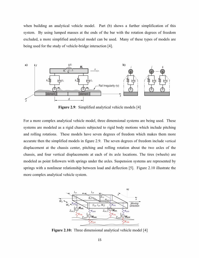
when building an analytical vehicle model. Part (b) shows a further simplification of this

system. By using lumped masses at the ends of the bar with the rotation degrees of freedom

excluded, a more simplified analytical model can be used. Many of these types of models are

being used for the study of vehicle-bridge interaction [4].

element j element ix

y

z

Rail Irregularity ( )r x

kv kv cvcv

θv

Mv

mv mv

yv

Iv

d

v

a)i j k

b)

Figure 2.9: Simplified analytical vehicle models [4]

For a more complex analytical vehicle model, three dimensional systems are being used. These

systems are modeled as a rigid chassis subjected to rigid body motions which include pitching

and rolling rotations. These models have seven degrees of freedom which makes them more

accurate then the simplified models in figure 2.9. The seven degrees of freedom include vertical

displacement at the chassis center, pitching and rolling rotation about the two axles of the

chassis, and four vertical displacements at each of its axle locations. The tires (wheels) are

modeled as point followers with springs under the axles. Suspension systems are represented by

springs with a nonlinear relationship between load and deflection [5]. Figure 2.10 illustrate the

more complex analytical vehicle system.

KSRR

KTRR

KTRL

War

Wal

Lar Laf

KSRL

KSFR

KSFL

KTRR

KTRL

MAFR

MAFL

MARR

MARL

ZAFR

ZAFLZARL

ZARR

Moving Direction

θVX

θVYZYC

x

y

z

(IVX, I , MVY V)

Figure 2.10: Three dimensional analytical vehicle model [4]

15  

An analytical model was also created by the Florida Department of Transportation along with the

Florida International University in order to create an AASHTO HS20-44 truck. This truck has

11 degrees of freedom and was used to evaluate the dynamic response of highway girder bridges.

Figure 2.11 illustrates the complexity in this system.

Ksy5 Dsy5 Ksy3 Dsy3 Ksy1 Dsy1

TractorTrailer

Kty5 Dty5 Kty3 Dty3 Kty1 Dty1

ya1ya2ya3

yt2 yt1

θt1θt2

Ksy1 Ksy2Dsy1 Dsy2

Kty1 Kty2Dty1 Dty2

yt1

θt1

ya1θa1

Figure 2.11: Analytical model of an AASHTO HS20-44 truck [4]

Analytical models of this type are treated as a multi-body system which is ideal for studying the

vehicle-bridge interaction theoretically. However, the number of degrees of freedom is limited

for mathematical convenience only. Since most parts of these analytical models are assumed to

be rigid, finite element software is needed to for the additional modeling of non rigid bodies.

Finite element modeling becomes extremely convenient for modeling complicated parts such as

the transmission, suspension system, etc. Very often, FE models are available in the public

domain for immediate use. These models are the most reliable because they consist of more

structural components then any other type of analytical vehicle model thus far. Components that

are included in these models are extremely detailed representations of the suspension systems

and kinematical characteristics of components and wheel models with airbags applied [5]. These

models are mostly developed for crashworthiness analysis but, can also be used when studying

vehicle-bridge interaction. Examples of FE models are available on-line (Finite Element Model

Archive, 2008) are presented in Figure 2.12.

The Crashworthiness and Impact Analysis Lab decided to utilize an already existing vehicle

model of a tractor-trailer in order to make additional modifications for a vehicle-bridge

interaction study. The tractor-trailer Mack CH613 with a three axle single drop lowboy trailer

was selected as a representative for the vehicle-bridge study. This vehicle was selected due to

the fact that it is the most popular truck in the United States. The complete FE model consists of

16  

over 25,000 finite elements. Blueprints and data from the manufacturer’s website were used for

the development of the FE model. The following components were included in the FE model

once the necessary modifications were made. These components include:

• a chassis, including complete wheels with elastic tires, simplified front single axle,

rear tandem axles, and suspension systems;

• a complete frame, including longitudinal frame rail and transverse beams,

e.g. cross-members, engine support beam, etc.;

• a fifth wheel.

Figure 2.12: Finite element models available in public domain [4]

In addition to all the necessary modifications, a load configuration was created to go on back of

the lowboy trailer. This additional load was distributed evenly on the load and top deck of the

trailer. The reason for this additional loading is to represent the heavy cargo that is commonly

carried when these types of trucks travel along highway bridges. Figure 2.13 illustrates the

completed FE model of the tractor-trailer used in the previous vehicle-bridge study, BD 493

contract.

Figure 2.13: FE model of the tractor-trailer and lowboy [5]

17  

CHAPTER 3

SELECTION OF OBJECTS FOR TESTING   

 One of the main objectives in this research is to analyze the effects of vehicle-bridge interaction.

In order to do this a FE model of a highway bridge was developed along with FE models of

heavy trucks. Under the BD 493 contract, FE models of three vehicles and an AASHTO Type

III girder bridge were created and validated for the Florida Department of Transportation. The

information from this contract will aide in obtaining the necessary information in order to verify

and validate a new bridge model with AASHTO Type II girders.

The use of existing finite element models of the vehicle were adopted from the previous contract

[5]. No modifications were performed to these models since the focus of the research deals with

the improvement of the bridge model. Three vehicle models were created under the previous

contract but only two of the vehicles were used for purpose of analyzing the dynamic behavior

between vehicle-bridge interactions. The decision on which vehicles to use were based on the

results from the BD 493 contract as well as the parameters and weight of the modeled trucks.

3.1 Use of Existing FE Model of Vehicles

Under the BD 493 contract, three vehicles of heavy trucks were carefully selected and validated

for use by the Florida Department of Transportation. Selection of these vehicles was based on

the following criteria [5]:

• Heaviest vehicle permitted for crossing bridge #500133

• Relatively small outer bridge length which is defined as the distance from the steering

axle to the last axle of the vehicle.

By taking these factors into account, this allowed one to obtain results for the worst case

scenario. Based on information obtained from the FDOT Permit Office the gross weights of the

heaviest vehicles permitted for crossing bridge #500133 were 90,265 kg, 89,358 kg, and

77,111 kg (199,000 lb, 197,000 lb and 170,000 lb respectively).

18  

For this project one vehicle was selected and was used in the study in order to analyze the

dynamic effects of vehicle-bridge interaction. Selection of this vehicle was based on the

following criteria:

• Results obtained from the previous project

• Information regarding the parameters and weight of each vehicle

Finite element models of the Tractor-Trailer truck were used for this study. The Tractor-Trailer

was used due to it being the longest in length and the heaviest in weight.

Once the decision was made to use this model, an assessment of the models had to begin in order

to make sure it was still accurate and reliable. Assessment of this model included several

analytical simulations. These simulations were done in order to ensure that the results would be

consistent with what was obtained two year ago, when the project was originally completed.

Once these models were verified, they were stored away for later use with the new bridge model.

Figure 3.1 provides pictures along with a detailed drawing of the selected vehicle for this project.

Figure 3.1: Detailed sketch of a Mack CH613 Tractor-Trailer truck [5]

 

Figure 3.2. Mack CH613 Tractor-Trailer truck [5]

19  

3.2 Selection of Highway Bridge

One of the main objectives of this research is to develop a finite element model of a new bridge

by modifying an already validated model developed previously for the Florida Department of

Transportation. When selecting the new bridge for modeling the same criteria was used for the

selection of the previous bridge. The main difference is that the new bridge could not have

AASHTO Type III prestressed girders. The reason for this has to do with the focus of this

research. In order to see if we can modify an already existing finite element model to represent a

new bridge model, it is important not to have the same girder type. Girders are one of the main

parts to a beam bridge and modeling AASHTO Type III girders, even if the bridge dimensions

were different, would be redundant for this purpose. For this reason an AASHTO Type II bridge

was used for the new model.

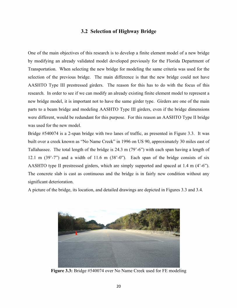
Bridge #540074 is a 2-span bridge with two lanes of traffic, as presented in Figure 3.3. It was

built over a creek known as “No Name Creek” in 1996 on US 90, approximately 30 miles east of

Tallahassee. The total length of the bridge is 24.3 m (79’-6”) with each span having a length of

12.1 m (39’-7”) and a width of 11.6 m (38’-0”). Each span of the bridge consists of six

AASHTO type II prestressed girders, which are simply supported and spaced at 1.4 m (4’-6”).

The concrete slab is cast as continuous and the bridge is in fairly new condition without any

significant deterioration.

A picture of the bridge, its location, and detailed drawings are depicted in Figures 3.3 and 3.4.

Figure 3.3: Bridge #540074 over No Name Creek used for FE modeling

20  

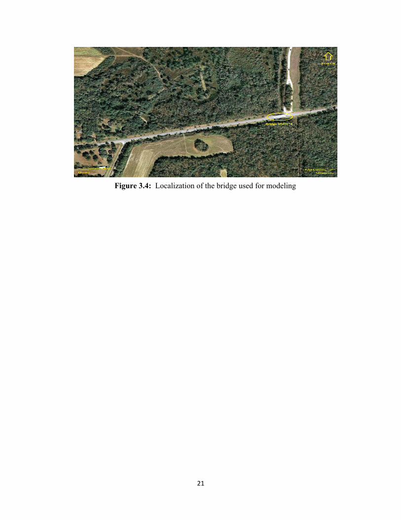
Figure 3.4: Localization of the bridge used for modeling

21  

CHAPTER 4

DEVELOPMENT OF FINITE ELEMENT MODEL

A completely new FE model of a bridge was developed for this research by performing all the

necessary geometric and material adjustments to a FE model developed during the previous

FDOT project: Investigation of Impact Factors for Permit Vehicles – FDOT Project No. BD543

[5]. The bridge that was modeled under this project was successfully created, verified, and

validated a concrete bridge in Chattahoochee, Fl. The new FE model took advantage of the

already existing bridge model in order to create a new bridge model which is located in

Tallahassee, Fl. The only major difference between the Chattahoochee bridge model and the

Tallahassee bridge model are in the girders. Since girder size governs the behavior of these

bridges, it is important to pay special attention to this part when modeling the new bridge.

FEA consists of a computer model that is stressed and then analyzed for specific results. Results

were used for new product design and existing product refinement. Today, nonlinear finite

element methods are commonly used in order to solve complex engineering problems.

In finite element analysis the prediction of structural performance and the modeling of girder

members under moving vehicle loads are essential in any bridge design. Since moving vehicles

cause an additional dynamic effect on bridges, this dynamic effect was accounted for in terms of

a dynamic load allowance. Dynamic Load Allowance (DLA) can be defined in several ways [7]:

• Definition 1: the difference in the maximum instantaneous dynamic response and static

response divided by the maximum static response.

• Definition 2: divide the dynamic response that occurs at the same location as the

maximum static response by the maximum static value.

• Definition 3: divide the maximum dynamic response by the static response that occurs

simultaneously with the maximum dynamic response.

For this research, definition 1 is used since it is the most rational definition for this type of study.

This is because, in design, the maximum static effect is scaled to give the maximum dynamic

effect regardless of when the two responses occur [18].

22  

In order to study and validate the dynamic response of a highway bridge with a medium span

(20-30 m) or (65-98 ft) subject to moving loads, finite element analysis was the chosen approach.

Emphasis was placed on the development of a finite element (FE) model of a selected highway

bridge by adopting an already existing bridge model and making all the necessary modifications

in order to get a newly modeled bridge.

4.1 Geometric Development of Existing FE Model

The FE model was developed using LS-PrePost, an interactive and commonly used pre-

processor for LS-DYNA. All necessary parameters including boundary conditions, element

properties, material properties, solution type, and many others were defined using this pre-

processor. Once the necessary modifications were complete, a key file was created in order to

save the model and export to LS-DYNA. The latest available version 971 of the LS-DYNA was

used for the FE analysis [19]. Preliminary analyses, including simulations with the isolated FE

models of the vehicles, were performed on 8 GB workstation with 4 Dual-Core processors. A 32-

node cluster was used when a large number of finite elements and long real time analyses were

required for a complete vehicle-bridge interaction study [5].

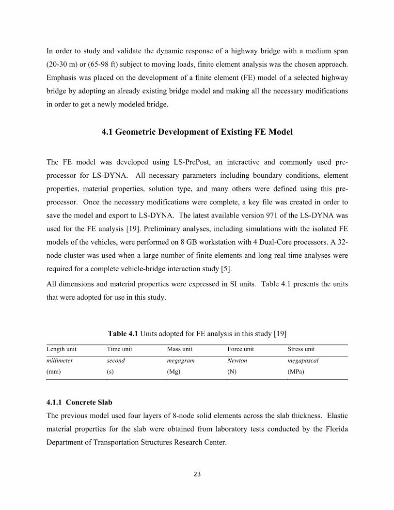
All dimensions and material properties were expressed in SI units. Table 4.1 presents the units

that were adopted for use in this study.

Table 4.1 Units adopted for FE analysis in this study [19]

Length unit Time unit Mass unit Force unit Stress unit

millimeter

(mm)

second

(s)

megagram

(Mg)

Newton

(N)

megapascal

(MPa)

4.1.1 Concrete Slab

The previous model used four layers of 8-node solid elements across the slab thickness. Elastic

material properties for the slab were obtained from laboratory tests conducted by the Florida

Department of Transportation Structures Research Center.

23  

The new model consists of the same material parameters because modification of the material

properties may cause inconsistencies in the results. Since the previous bridge model has already

been successfully validated, staying consistent with the element and node count in the

modification process is important. This will ensure that there are no inconsistencies when

creating the new bridge model. The first step in creating the new model was the modification of

the span length and width. A scale factor of 1.37 was used to edit the span length along with a

scale factor of 1.15 for the span width. Figure 4.1 shows the concrete slab of the existing model

and of the new model.

a)

b)

Figure 4.1. FE model of concrete slab with LS-Dyna summary: a) existing bridge model, b) modified bridge model

24  

Despite the noticeable difference in the concrete slab, it is important that element count and node

counts remain the same. Table 4.2 shows the dimensions for both, existing and new, bridge

models.

Table 4.2. Summary of concrete slab model parameters

Model Type Span Length (m/ft) Span Width (ft) Element Count

Existing model 69 ft (21.0 m) 45 ft (13.1 m) 45360

New model 40 ft (12.1 m) 34 (10.2 m) 45360

4.1.2 AASHTO Type II Beams

The most important component in the alteration process is of the AASHTO beams (girders). A

concrete bridge is governed by the girder type that supports the concrete deck. Because of this

special attention was made when modifying this part. In the original model each beam includes

two No. 9 strands at the top and 24 No. 13 strands at the bottom. Only one equivalent strand at

the top and eleven equivalent strands at the bottom were modeled due to discrete location of the

nodes in the cross-section of the beam FE model. Selected strands were grouped and their

properties were distributed into equivalent ones to make sure that the FE model well represents

the real beam [5].

The new model encompassed these same material parameters when developing the AASHTO

Type II model from the AASHTO Type III. Table 4.3 summarizes the material properties of the

concrete beams.

Table 4.3. Material properties for concrete beams [5]

Specification Unit Value

Young's modulus, E (GPa) / (ksi) 37.5 / 5441.9

Poisson's ratio, ν — 0.22

Specify compressive strength, fc' (MPa) / (ksi) 63.7 / 9.24

The first step in the modification of the concrete beam is to figure out the dimensioning of an

AASHTO Type II girder. Figure 4.2 shows the dimensioning of the cross section of an

25  

AASHTO girder. Once this is done, the Scale command can then be used in order to get the

desired dimensions.

The Scale command was the most useful geometric tool in LS-PrePost. This command allowed

the scaling of selected elements. The scaling direction and factor can be specified using various

methods for maximum flexibility to suit different users needs [19]. The scale factor was

determined by taking the previous model location of the node and subtracting it from the location

of where the new nodes should be for the new model. Once that difference is calculated, divide

the difference by the original model location. The direction of scaling was decided upon by the

direction of the previous model in order to keep consistency. This procedure was done very

carefully and methodically until all the girder nodes of the existing model were in the location of

where the new girder nodes should be. Equation 4.1 displays the formulas used for scaling all

nodes.

SF 4.1

NE is the node location of the existing model and NM is the location of the new model. Equation

4.1 is a standard algebraic equation that is often used to find the percent difference in science and

math.

a) b)

Figure 4.2: AASHTO girder dimensions:

26  

Once dimensions have been established the editing can begin. The z-direction were the first

direction used for scaling. This direction is important because it takes into account the

modification of the web. Once scaling in the z-direction is completed, the same procedure was

used to scale the y-direction. The y-direction focused on the modification of the flange as

oppose to the web. The dimensions of both type II and III AASHTO girders are illustrated in

Figure 4.3. The only direction that was not taken into account is the x-direction. This direction

was automatically scaled due to the scaling of the bridge span which occurred in the x-direction.

Figure 4.3. Girder modification in z-direction: a) Existing model,

b) Modified model

The lengths are expressed in millimeters. It is important to note that the nodes that were selected

for measuring are the same for both the existing model and the new model. For this type of

research, it is important to have the same nodes as the existing model. This ensures consistency

when creating the new model from the previous one. This also ensures that there is no depletion

or addition of nodes or elements throughout the modification process. The girders in the new

bridge model are of an AASHTO Type II girder. It is easily seen that the previous model is

larger due to the type of girder that was being used to model that specific bridge, AASHTO Type

III.

27  

Other commands allowed for scaling in the XY, XZ, and YZ directions. These directions lie

along the angles of the girders cross section. Scaling of the angles will occur in the same manner

you would when scaling along an orthogonal direction. Scaling of the angles were done last due

to the fact that after scaling in the Y and Z direction were completed, most of the nodes in the

YZ direction took care of themselves and automatically scaled themselves into the right position.

Once all scaling of the nodes were completed, a new model of the bridge deck and girders were

then combined in order to begin the creation of the new bridge model. The complete FE model

of the new and existing girders is presented in Figure 4.4.

Figure 4.4. FE Model of completed girder modifications: a) Existing model, b) Modified model

28  

Traffic Railing Barriers

The previous bridge model used 3D solid, fully integrated elements in order to model a concrete

barrier. The new model will utilize the same procedure used to model the barrier in the previous

model. The barrier length is the only modification that had to be done. The reason for this is due

to the fact the railing barriers has the same cross section as the new bridge model. The only

dimension that needs to be modified is the span length. A traffic railing barrier needs to run

along the span of the bridge. Since the span length between the existing and the new bridge

model are different, the barrier length needed to be scaled down to the length of the new bridge

span. In order to successfully scale down the barriers, the end nodes of the concrete deck should

be used as a reference point.

Once scaling of the desired length is completed, the Translt command is then utilized. The

purpose of this interface is to simply translate selected nodes to their appropriate location. The

direction and distance can be specified using various methods for maximum flexibility in order

to suit different user needs [19]. By using the points (nodes) on the coordinate system, one can

simply locate the node position on the existing model and translate it to the desired location on

the same coordinate system. The distance between those two points is considered as the

translation distance and should be used when translating selected nodes.

The FE model of the traffic railing barrier is presented in Figure 4.5. The Measure interface was

used in order to verify that the length of the barriers was in fact modified. This technique also

verifies that the span length of the bridge was also modified since traffic railing barriers are

constructed to be the same length as the concrete deck.

29  

Figure 4.5: FE Model of traffic barrier railings: a) Existing model, b) Modified model

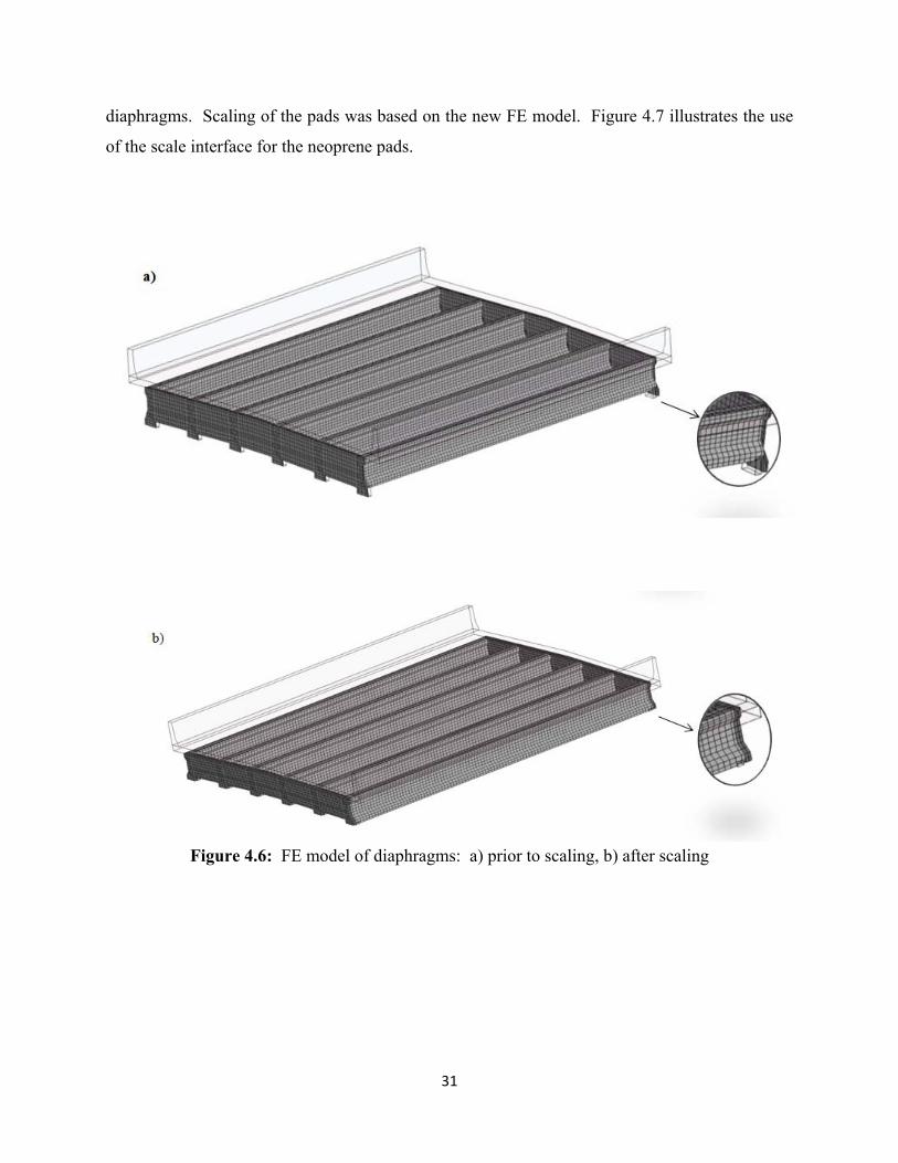
Diaphragms

Concrete diaphragms for the new bridge model will be made up of 3D solid elements just like

what was used in the previous bridge model. The Scale interface will be useful in modifying the

concrete diaphragms. Once girder modifications were completed, they served as an outline for

where the diaphragms needed to go. Due to this, the existing model was no longer needed for

modification assistance. By locating the node points along the girder of the new model, the

diaphragms were scaled down to the desired node location. Figure 4.6 illustrates how the

diaphragms were modified without the assistance of the existing model.

Elastomeric Bearing Pads

The main focus of the new bridge was in the neoprene pads, a subset of elastomeric bearing

pads. These pads are used to support each girder on bridge piers. Special attention was made to

the modification of these pads since this is the focus of improvement for this research. Solid

elements were used to model these parts in the previous model and will be utilized for the new

model. Dimensions for the neoprene pads were identified by the Florida Department of

Transportation Specifications for pads supporting AASHTO Type II girders. Once the

appropriate dimensions were identified, the Scale interface was used in the same manner as the

30  

diaphragms. Scaling of the pads was based on the new FE model. Figure 4.7 illustrates the use

of the scale interface for the neoprene pads.

Figure 4.6: FE model of diaphragms: a) prior to scaling, b) after scaling

31  

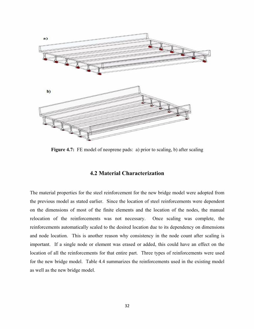
Figure 4.7: FE model of neoprene pads: a) prior to scaling, b) after scaling

4.2 Material Characterization

The material properties for the steel reinforcement for the new bridge model were adopted from

the previous model as stated earlier. Since the location of steel reinforcements were dependent

on the dimensions of most of the finite elements and the location of the nodes, the manual

relocation of the reinforcements was not necessary. Once scaling was complete, the

reinforcements automatically scaled to the desired location due to its dependency on dimensions

and node location. This is another reason why consistency in the node count after scaling is

important. If a single node or element was erased or added, this could have an effect on the

location of all the reinforcements for that entire part. Three types of reinforcements were used

for the new bridge model. Table 4.4 summarizes the reinforcements used in the existing model

as well as the new bridge model.

32  

Table 4.4: Dimensions for ASTM standard reinforcing bars used in bridge structures [5]

Bar Size Designation Mass

(kg/m) / (lb/ft) Diameter

(mm) / (in) Area

(mm2) / (in.2)

10M 0.785 / 0.527 11.3 / 0.445 100 / 0.155

15M 1.570 / 1.055 16.0 / 0.630 200 / 0.310

20M 2.355 / 1.582 19.5 / 0.768 300 / 0.465

Material properties for the reinforcement of the concrete slab were obtained from laboratory test

conducted by the FDOT Structures Lab. Two types of the reinforcing bars were used in the slab

structure – size 10M and 15M. They were modeled using 1D beam elements with the elastic

material model applied. The material properties for the entire slab are presented in Table 4.5.

Table 4.5: Material properties of the concrete slab [5]

Specification Unit Value

Young's modulus, E (GPa) / (ksi) 40.5 / 5871.8

Poisson's ratio, ν — 0.20

Specify compressive strength, fc' (MPa) / (ksi) 55.9 / 8.11

The material for the reinforced concrete barriers consisted of 10M and 15M reinforcing bars. 1D

beam element with elastic material properties was used. The cross-section of the concrete

barriers with reinforcing bars is presented in figure 4.8.

Figure 4.8: Cross-section of traffic railing barriers [5]

33  

Material properties for the beam are presented in Table 4.6. Each beam includes two No. 9

strands at the top and 24 No. 13 strands at the bottom. Only one equivalent strand at the top and

eleven equivalent strands at the bottom were modeled due to discrete location of the nodes in the

cross-section of the beam FE model. Selected strands were grouped and their properties were

distributed into equivalent ones to make sure that the FE model well represents the behavior of a

girder. A special material model type 071 (*MAT_CABLE_DISCRETE_BEAM) was applied

in order to introduce prestressing force in the rod elements. Material properties used for the

concrete girders are listed in Table 4.6.

Table 4.6: Material properties for concrete girders [5]

Specification Unit Value

Young's modulus, E (GPa) / (ksi) 37.5 / 5441.9

Poisson's ratio, ν — 0.22

Specify compressive strength, fc' (MPa) / (ksi) 63.7 / 9.24

Concrete diaphragms for the bridge included reinforcing bars represented by 1D beam elements.

Figure 4.9 shows the complete FE model of the bridge with only the steel reinforcement bars

visible. Due to the fact that the previous research used the location of the rebar based on the

node location of the model, all rebar were automatically scaled to the desired location once the

necessary geometric modifications occurred.

Figure 4.9: FE model of reinforcements

34  

Since this research focuses on the improvement of the bearing pads, this was the only part in the

new model that was subjected to material modifications.

4.3 Importing of Key File

Imported files added data to a current model. This process is essential when time constraints are

of the essence. In order to import a file, it must first be saved as a key file using LS-Prepost.

The data that is added to an already existing file must be redefined. This is one of the most

important steps when importing a key file due to the lack of correlation once a key file has been

imported into another key file. The parameters that need to be redefined in order to have a

successful simulation are as follows:

• Part ID/Node ID

• Boundary Condition

• Constraint

• Contact

• Load curve

Once the key file of the new bridge model was completed and saved it was then imported into an

already existing key file. The existing key file is of a bridge with AASHTO III girders along

with a FE model of an already validated vehicle. The first step in the importing process is to

remove the already existing bridge. Once this bridge has been successfully deleted from the

existing vehicle-bridge model, the new key file of the AASHTO II girder bridge can then be

imported in order to replace the removed bridge. Data from the new bridge model will override

the previous data hence, redefining of parameters in certain interfaces is essential in order to get

the model to work. Interface definitions are used to define surfaces, nodal lines, and nodal points

for which the displacement and velocity time histories are saved at some user specified

frequency [LS-Dyna Manuel]. The interface feature represents a powerful tool for LS-Dyna

analysis capabilities.

The *Part interface is crucial in the redefining of the parameters. This interface relates part ID

to the *SECTION, *MATERIAL, *EOS and *HOURGLASS sections. Since the new bridge

model was developed using different Part IDs, the LS-Dyna will not recognize the parts of our

35  

new bridge model. In fact, if the key file were to run as is, an error would occur right away

stating:

• Warning - MAT 7703 not found: Referenced in *Part ID index = 4351.

• Warning - SEC 3800 not found: Referenced in *Part ID INDEX = 4351.

These errors were common in the initial attempts to run the new model. The first part of the

warning message is telling the person that there was a problem finding that particular ID number

for that specific interface. This could be due to the fact that nothing has been redefined

therefore, LS-Dyna is not able to read these ID numbers or, ID numbers got erased when deleting

the old bridge model. In any case investigation on these errors must be sought out in order to get

the model to run and yield accurate results. The second part of the error message has to do with

where this error can be found. The two previous bullets indicate that both errors dealing with the

material and section can be found in the *Part interface, specifically ID number 4351. Figure

4.10 displays the *Part interface dialog box that is used to define the section and material that is

dependent on the PART ID. The *EOS and *HOURGLASS are not defined in this interface for

this particular study.

Figure 4.10: *Part interface dialog box for LS-Dyna

36  

Another common warning message had to do with errors pertaining to boundary conditions and

constraints. The *Boundary interface applies various methods of specifying either fixed or

prescribed boundary conditions. The prescribed boundary condition deals with any boundary

conditions that has motion. This specific interface did not need to be redefined or altered due to

the fact that all prescribed boundary motion was applied to the vehicles only. Since the vehicles

were not imported, the data remains the same and there is no need for changes. On the other

hand, the fixed boundary conditions were applied to the bridge thus, modification of this

interface was needed. In order to fix errors pertaining to boundary conditions, node sets had to

be redefined first in order for recognition by LS-Dyna. Once that was completed the proper

boundary conditions were applied to the new redefined NODE_SET.

The *Cnstrnd interface is used to apply constraints within the structure between structural parts

[22]. For this research, constraints were applied as joints. Since the joints were applied solely to

the tractor-trailer and the crane, there was no need to go into this interface for redefining. Figure

4.11 illustrates the joint that were used for this study. If the imported key file was of a vehicle

rather than a bridge, joint constraints would certainly need to be looked into and redefined if

necessary.

Another interface that needs to be successfully modified in order for a simulation to occur are

issues pertaining to the *Contact and the *Define interface. Since the new imported bridge

model will be in contact with the existing vehicle models, these interfaces are vital in the

modification process. The *Contact interface allows the user to define contact options for

treating of deformable to deformable bodies, single surface contact in deformable bodies,

deformable rigid body contact, and tying deformable structures with an option to release the tie

based on plastic strain [22]. The most frequent error message resulting from contact issues were

as follows:

• Warning – Multiple contact label # 1- This may lead to confusion when viewing the

output.

• Warning – Error node set for extra node for rigid body # 7.

The first error message lets the user know that there are multiple contact definitions that

coincides with the first contact definition. The second part of the error message lets the user

know that this is confusing LS-Dyna and needs to fixed in order to run the file. Instead of

redefining parameters, all that is needed is the removal of any multiple contact card with the

37  

exception of #1. This error occurs simply because when the key file is imported, extra data is

added to the already existing model. That is why issues concerning the multiple of any card

exist. The same principal applies to the second warning message, Error node set for extra node

for rigid body. The depletion of any duplicate node set that surfaced due to the importing of the

key file must be deleted so that there is no confusion. The *Define interface allows users to

define curves for loading, constitutive behavior, etc. [22]. This interface allows for the vehicle-

bridge interaction to take place. This is one of the most important interfaces when dealing with

motion. Without this interface, the vehicle would not know where to go, how to get there, or

even how to behave once it reaches the bridge. Common error messages for this interface were

as follows:

• Warning – DEFINE_CURVE 10 not found: Referenced in

*MAT_SPRING_NONLINEAR_ELASTIC id = 4641

• Warning – DEFINE_CURVE 11 not found: Referenced in

*MAT_DAMPER_NONLINEAR_VISCOUS id = 4642

The first error message states that LS-Dyna cannot find curve # 10 which is located in the

*Material interface under the nonlinear elastic spring card. In order to fix this error the

nonlinear elastic spring card must be pulled up under the *Material interface for modifying. In

this particular case id # 4641 only needs to be removed not redefined. This is because id #4641

is added data from the new model which is why LS-Dyna cannot find it. Once that id is

removed, LS-Dyna no longer reads it and can now continue with the simulation. The same idea

applies to the second warning message.

The *Dbase interface is used for controlling the output of ASCII databases and binary files

output by LS-Dyna. This interface defines the frequency for which the writing of databases

occurs. The D3PLOT card is one of the most important section in this study because this is

where the results are stored. This command contains plotting information to plot data over the

three dimensional geometry of the model. The D3THDT card contains files with time history

data for element subsets as well as global information. Since this study focuses on the validation

and verification of a new and existing FE model, keeping this interface the same, with no

changes, will allow for consistency between both sets of binary output files.

A total of 182 errors were found once the new file was imported into the already existing file.

These errors had to be dealt with systematically in order to decrease the error count rather than

38  

create new ones. Figure 4.12 illustrates an actual error report that occurred throughout the

modification process once the new bridge model was imported onto the existing vehicle model.

Understanding error reports once a file has been submitted is essential in the development

process of a FE model. Once all errors have been successfully corrected, LS-Dyna will produce

a normal termination report, which signals to the user that the key file was successfully in the

analysis process and is ready for a simulation.

Once all the simulations were finished and the model was ready for analysis the following

summary information for the bridge model, No Name Creek is presented in Table 4.7.

a) b)

Figure 4.11: LS-Dyna error reports: a) error termination report, b) normal termination report

39  

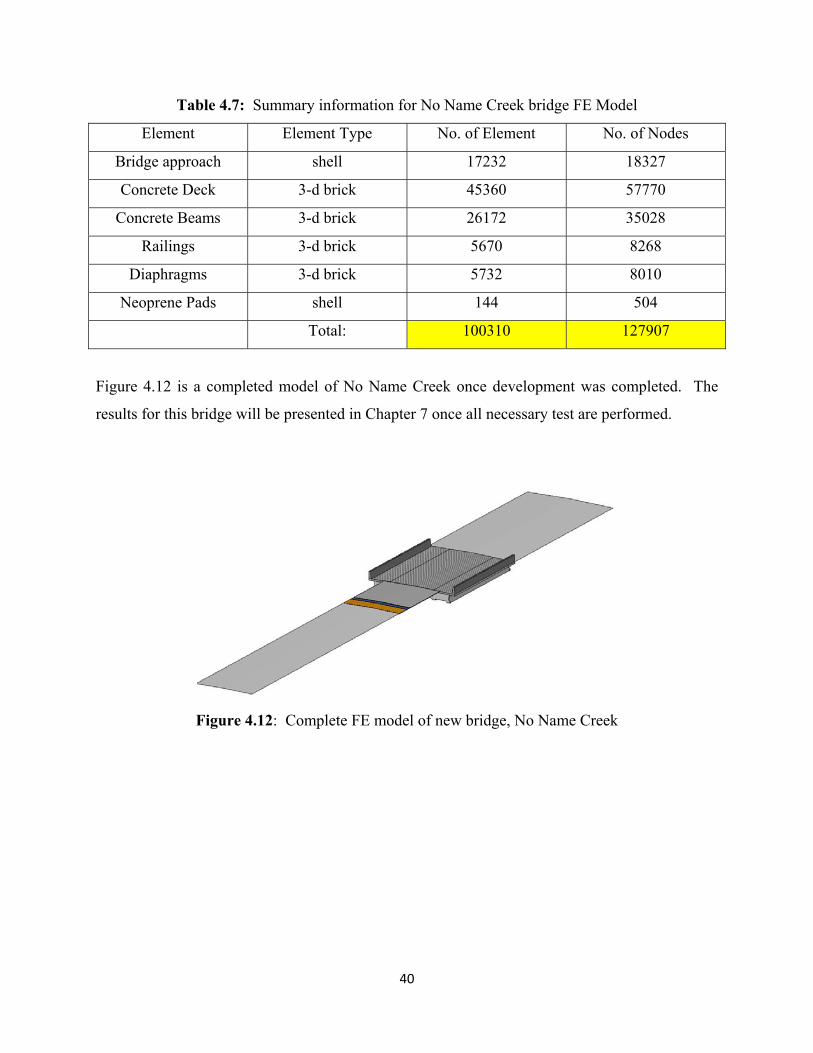
Table 4.7: Summary information for No Name Creek bridge FE Model

Element Element Type No. of Element No. of Nodes

Bridge approach shell 17232 18327

Concrete Deck 3-d brick 45360 57770

Concrete Beams 3-d brick 26172 35028

Railings 3-d brick 5670 8268

Diaphragms 3-d brick 5732 8010

Neoprene Pads shell 144 504

Total: 100310 127907

Figure 4.12 is a completed model of No Name Creek once development was completed. The

results for this bridge will be presented in Chapter 7 once all necessary test are performed.

Figure 4.12: Complete FE model of new bridge, No Name Creek

40  

CHAPTER 5

ELASTOMERIC BEARING PADS

The American Association of State Highway and Transportation Officials (AASHTO) published

guidelines for the design of highways that include design specifications for bridge bearing pads.

Composite pads, also known as laminated bearing pads or reinforced pads, are made by bonding

layers of an elastomeric material with layers of reinforcement which typically consist of thin

steel plates. AASHTO recommends using steel plates as reinforcement because they carry the

greatest vertical loads [25].

This chapter focuses on the identification of material and geometric characteristics, in order to

get a better correlation between the analytical results and the experimental results. A geometric

study as well as a material characteristic study was performed in order to develop an ideal pad. In

order to design a pad with improvements from the existing bridge model pad, several factors

needed to be studied. The design of the pad was the first step for improvement followed by the

material properties. For simplicity, the material properties were broken down into 3 cases in

order to analyze the improvement of each case separately. The reason for focus on this particular

part of the bridge has to do with the fact that neoprene pads are simple solid pads with no

moving parts which makes them straightforward when creating finite element models for them.

The stiffness of these elastomeric bearing pads affects the dynamic response of the

superstructure, since it changes the natural frequency of the superstructure which influences the

vehicle-bridge interaction. Hence, elastomeric bearing pads are of significant importance. These

pads are also economical, effective and require no maintenance which makes them ideal for

improvements. A parametric study was performed on the material properties as well as the

geometric properties. The parameters studied include the shear modulus, Poisson ratio, and

shape factor. The FDOT has provided a detailed sketch of the recommended dimensions for

bearing pads on Florida highway [12]. This study will stay consistent with the recommended

specifications but, the amount of layers will need to be determined in order to get the best

possible shape factor and to find its influence on the bridge dynamic response.

41  

The improvement of the elastomeric bearing pads were done by modifying an existing model.

Despite a successful validation by CIAL and the FDOT, special attention was made on

improving the bearing pads only. Since bearing pads are used to support dead and live loads,

allow for longitudinal movements and, accommodate girder rotation, a successful improvement

will allow for better support of the bridge therefore, minimizing its deflection.

The shape factor, defined as the plan area divided by the area of the perimeter free to bulge is the

most important geometric parameter of elastomeric bearing pads. The thinner the elastomer

layer, the larger the shape factor. The thickness and the plan dimensions of neoprene affect its

stiffness. For instance, with an increase in the thickness of the neoprene pads, its vertical

stiffness will decrease considerably [24]. The reduction in the vertical stiffness will decrease

significantly when reinforcement is added to each rubber layer. Hence, very close attention

should be paid to choosing these dimensions at the design stage. Since thinner layers provide for

more steel reinforcements, these pads are able to support larger loads and movements than a

plain pad, which has no steel reinforcements. In order to satisfy the compressive stress and shear

deformation criteria AASHTO recommends using the following equations presented in section

5.2 of this research. An assessment of the existing bearing pad model was also verified with this

data to ensure that the dimensioning was not an issue for error. Once dimensioning was

complete, a decision on the amount of layers was needed to be made in order to accurately

calculate the shape factor of the new bearing pads.

Another important parameter that needs to be taken into account when improving bearing pads

are the material parameters. These parameters are essential when analyzing the behavior of these

pads under certain loading conditions. Neoprene pads are subset of elastomeric bearing pads and

will be the material of chose in the improvement of these pads. Material properties for neoprene

rubber will be important in determining the main material parameter, the shear modulus.

In order to make improvements on the bearing pads, an analysis of the binary output files must

first be considered since this is how LS-Dyna produces results. If the outputs of these files are

not consistent with each other, it may cause issues with the verification and validation process.

Before any modification of the bearing pads can take place, an assessment of the existing model

must be done in order to verify that errors will not be due to inconsistencies. A problem with the

original model’s output was discovered during the assessment process. This problem was solved

prior to running simulations.

42  

The problem with the old model was that it did not run for the time that was defined in the

database interface. In other words, the model terminated earlier than what was defined by the

user. The model was defined to terminate at t = 5.00 seconds but, upon completion of the

assessment, the model terminated at t = 3.62 seconds. By going into the LS-PrePost database

and changing the way LS-Dyna calculated certain elements, the termination time of 5.00 seconds

was reached. Without this initial improvement, verification and validation of these time histories

may result in miscalculations.

Once the necessary modifications have been applied to the time history graph, focus on the

improvement of the actual bearing pads can begin. Listed below in Figure 5.1 are the time

histories of the original model once corrections to the element formulation and the database were

completed. Emphasis will be placed on the displacement and strains of the neoprene pad only.

The reason other parameters were not studied in this research is due to the fact that field results

for the bridge only took into account displacement results and strain results. Without accurate

field results for the bridge, validation was not able to be performed between the new bridge

parameters and existing field results. Once improvements of the pads were completed, they were

then put into 3 different cases. These cases were used as a way to keep track of the different

material properties used. Case 1 will adopt the material properties used in the original bridge

model, with no changes made. Case 2 and 3 adopted their material properties due to an analysis

method taken by AASHTO. Section 5.3 of this chapter discusses exactly how material

characteristics have an effect on the neoprene pads and the analysis involved in obtaining Case 2

and 3 material properties. Chapter 6 will take these material characteristics for all 3 cases in

order to see how the neoprene pads will affect the entire bridge model as a whole. Once this was

completed, Chapter 7 produced the overall dynamic load allowance for each of the cases.

From the graphs in Figure 5.1, both numerical displacements and strains yield maximum values

higher than the field results. The maximum deflection of the field results and the numerical

results are 1.39 mm and 3.13 mm respectively. The maximum strain for the field test and the

numerical test are 48.34 µm/m and 67.67 µm/m respectively. By improving on the elastomeric

pads one can conclude that the results of the numerical simulation will come closer to the field

results, which ultimately will reduce the dynamic load allowance of the vehicle-bridge

interaction in the finite element model.

43  

‐3.500

‐3.000

‐2.500

‐2.000

‐1.500

‐1.000

‐0.500

0.000

0.500

0.000 1.000 2.000 3.000 4.000 5.000 6.000

Deflection

 (mm)

Time (s)

Field Displacements

Numerical Displacements

‐10.000

0.000

10.000

20.000

30.000

40.000

50.000

60.000

70.000

80.000

0.000 1.000 2.000 3.000 4.000 5.000 6.000

Strain

 (m/m

)

Time (s)

Field Strain

Numerical Strain

Figure 5.1: Time histories of existing material pad parameters

The material characteristics that were used in the neoprene pads to determine the maximum

deflection and strain of the numerical model were as follows:

• Short-time shear modulus, GO = 17 MPa

• Infinite-time shear modulus, G∞ = 16 MPa

44  

• Elastic bulk modulus, K = 101 MPa

The goal of this study was to decrease the amount of displacement and strain in order to get

better correlation with the field results. One can see that there is in fact a difference between the

computational and the field results. By improving on the geometric and material characteristics

of the neoprene pad, one will see that the computational results will have a better correlation

with the field results. It is important to note that once the appropriate geometric improvements

were made, they were adopted in all 3 cases. The result of the actual geometric improvements is

presented in Section 5.1.

5.1 Improvement of Bearing Pad Design

There are two design methods that can be used to design steel reinforced elastomeric bearing

pads according to AASHTO Specifications. These methods are referred to as Method A and

Method B. Method B is the most current method and was recently added to the AASHTO

specifications. The Commentary of the AASHTO Specification states that Method B typically

results in a higher bearing capacity as well as smaller horizontal forces [25]. The Florida

Department of Transportation Specifications was reviewed in order to assess the current bearing

pad design. This information was useful in determining the size, design requirements, and

material grades for the new bridge model bearing pads. These dimensions are for pads designed

to support Type II to IV (AASHTO) beams in prestressed bridges. These values are listed in

Table 5.1.

Table 5.1: FDOT bearing pad dimensions for AASHTO beams [25]

45  

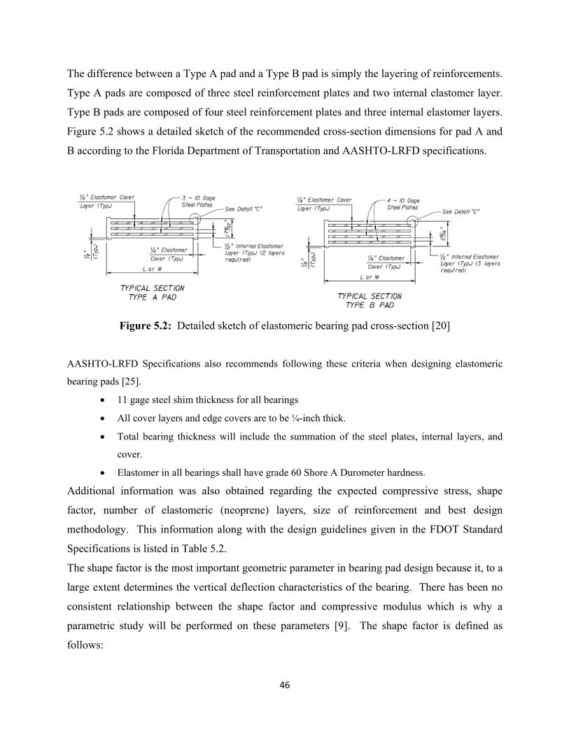
The difference between a Type A pad and a Type B pad is simply the layering of reinforcements.

Type A pads are composed of three steel reinforcement plates and two internal elastomer layer.

Type B pads are composed of four steel reinforcement plates and three internal elastomer layers.

Figure 5.2 shows a detailed sketch of the recommended cross-section dimensions for pad A and

B according to the Florida Department of Transportation and AASHTO-LRFD specifications.

Figure 5.2: Detailed sketch of elastomeric bearing pad cross-section [20]

AASHTO-LRFD Specifications also recommends following these criteria when designing elastomeric

bearing pads [25].

• 11 gage steel shim thickness for all bearings

• All cover layers and edge covers are to be ¼-inch thick.

• Total bearing thickness will include the summation of the steel plates, internal layers, and

cover.

• Elastomer in all bearings shall have grade 60 Shore A Durometer hardness.

Additional information was also obtained regarding the expected compressive stress, shape

factor, number of elastomeric (neoprene) layers, size of reinforcement and best design

methodology. This information along with the design guidelines given in the FDOT Standard

Specifications is listed in Table 5.2.

The shape factor is the most important geometric parameter in bearing pad design because it, to a

large extent determines the vertical deflection characteristics of the bearing. There has been no

consistent relationship between the shape factor and compressive modulus which is why a

parametric study will be performed on these parameters [9]. The shape factor is defined as

follows:

46  

S = (5.1)

where:

L = length parallel to the flow of traffic (mm)

W = width perpendicular to traffic flow (mm)

hri = height of individual elastomer layer (mm)

Table 5.2: Typical bearing properties [1]

In order to accurately model the new neoprene pads, a detailed sketch of the pads were obtained

by the FDOT Structures Research Center. Since the dimensions are the only definitive

parameter in this study, improvements will only be made to the layering and reinforcement of

these pads. AASHTO-LRFD recommends using a type A or type B pad when designing. Figure

5.3 shows a sketch of the existing neoprene pad used in the previous research.

The neoprene pad in the existing bridge model does not utilize steel reinforcements, Figure 5.3.

This pad was designed as a plain pad which resulted in a shape factor of 1.70. Table 5.2 shows

that the shape factor should fall in the range of 6 to 9. Therefore, the shape factor for the existing

bearing pad in the original model had to be improved. Figure 5.4 illustrates a Type A and Type

B design which is recommended by AASHTO. These design methods utilizes steel

47  

reinforcement as a way to strengthen the elastomeric pad. It is the more current form of pad

design and is vital for improving the shape factor.

Figure 5.3: Original neoprene pad used on existing FE bridge model

Figure 5.4: Improved neoprene pad for existing FE model; a) top pad, b) bottom pad

48  

Figure 5.4 shows that the cross section of the original pad, Figure 5.3, has no steel

reinforcements. This is the major difference between the original pad and the improved pad,

Figure 5.4. Since we only know the overall dimensions, it is important to perform a geometric

parametric study in order to figure out the exact dimensions of the cross section. The parametric

study was done in order to determine the internal elastomeric layer height. The internal layer

height is a key factor in determining the shape factor for the pads and therefore must be studied

carefully.

In order to begin analysis on the neoprene pad certain issues concerning the dimension tolerance

had to be considered. The tolerance is defined as the permissible variation from the dimensions

and configuration shown on the plans. Table 5.3 lists all the permissible variations for laminated

elastomeric bearing pads. The internal elastomer layer height, hri is significant in determining

the shape factor of the new bearing pad thus; the length and width are considered to be fixed in

this study. Hri will be the only geometric parameter that will need further investigation in order

to determine the ideal design. Once the ideal parameters are chosen a parametric study was

conducted in order to determine whether Type A or Type B pad is the better design. The result

of the study was used not only to improve on the existing model but, will also be implemented in

the new bridge model. This will ensure that the new bridge model utilizes the best geometric and

material parameters.

Since we already know the overall dimension of the pads, the tolerance was used only when

necessary. The parametric study helped in determining whether or not tolerance was an issue.

Given that the width and height are fixed, the internal layers were modified in order to obtain a

better shape factor for the existing neoprene pad design. A geometric parametric study was done

in order to investigate the variation of the internal elastomeric layer with the shape factor. Figure

5.5 shows a graph of how the shape factor changes depending on the internal layer thickness.

This will be vital information in determining the shape factor since it is based extensively on the

internal layer thickness.

The effect of variation of the internal elastomeric layer with the shape factor varies

hyperbolically. As the internal layers become larger, the shape factor gets smaller. This will

happen until the shape factor approaches zero.

When this happens, the neoprene laminated bearing pad becomes a plain pad with no internal

layering for reinforcements. On the other hand, having an internal layer equivalent to 1

49  

millimeter produces a shape factor approximately equal to 47.0. This is also not realistic since a

design like this would not be considered economical due to the amount of steel reinforcements

that would be needed every 1 millimeter.

Table 5.3: Dimension tolerance for bearing pads [23]

0.00

5.00

10.00

15.00

20.00

25.00

30.00

35.00

40.00

45.00

50.00

0 1 2 3 4 5 6 7 8 9 10 11 12 13

Shape

 factor,

 S

Internal layer height, hri (mm) 

Shape Factor

Figure 5.5: Graph of shape factor vs. internal layer thickness

50  

The results of the parametric study of the shape factor and the internal height are listed in Table

5.4. The table on top are the values recommended by AASHTO and FDOT thus, must remain

fixed. The fixed height which is given as 45 mm. is important in this parametric study due to the

fact that this is the ideal height that should be obtain in the end of the parametric study. If the

height of the pad does not equal 45 mm, the study becomes invalid since it would no longer

acknowledges AASHTO or FDOT specification recommendations.

Table 5.4: Result of geometric design

Type Layers Length (mm) Width (mm) Internal Height

(mm)

Shape

Factor

Total Height

(mm)

A 3 458 230 12 6.38 45

B 4 458 230 7 10.94 45

The result of the geometric study, Table 5.3, yields a Type A design which resulted in three

layers of steel with each layer spaced at 12 mm., produced a shape factor of 6.38. On the other

hand, the Type B design yields 4 layers of steel with each layer spaced at 7 mm., which resulted

in a shape factor of 10.94. At first glance, Type B seems to be the ideal choice due to its larger

shape factor but, this may be considered to be too conservative and therefore not economical.

Table 5.2 states that the appropriate shape factor for standard AASHTO beam sizes should fall

between 6 and 9. Because of this statement, Type B was omitted and Type A was chosen as the

ideal geometric design for this study.

The result of Type A, which results in a shape factor of 6.38, is shown below in Figure 5.5. You

can see from this graph that the hyperbolic relationship holds true, as predicted earlier in Figure

5.4. Again, an internal layer of 1 mm. produces a shape factor of 76.56 which is very high but,

way too conservative thus, not practical. On the other hand an internal height of 45 mm, which

is the same as the plain pad design, produces a shape factor of 1.70 which is too low and is why

improvements are needed. The internal heights can be seen in Figure 5.6. The spacing between

the steel reinforcements is considered the internal height of the neoprene pads.

51  

0.00

10.00

20.00

30.00

40.00

50.00

60.00

70.00

80.00

90.00

0 10 20 30 40 50

Shape

 factor,

 S

Internal layer height, hri 

Parametric Study for Shape Factor

Parametric Study for Shape Factor

Figure 5.6: Graph of geometric study

The initial parametric study shows that if a Type A pad is used as the basis for design, a shape

factor of 6.38 is produced. This is a vast improvement from the plain pad design in the original

bridge model of 1.70.

5.2 Analysis of Bearing Pad Improvements

Asides from the bearing pad design, the most important consideration are the material properties.

The neoprene pads used for this study were modeled using a viscoelastic material. This material

contains both elastic and viscuous components. The deformation of viscoelastic material is

dependent on load, time, and temperature. For the sake of our investigation, temperature will be

ignored and assumed to be the standard temperature of 73°, AASHTO-LRFD S14.7.4.2. For

simplicity, we will only consider limiting values of shear at very short and very long times.

Currently, our viscoelastic material has properties as follows:

1. Relative Density, (RO) = 1.3 x 10-9

2. Elastic Bulk Modulus, (K) = 101

3. Short Time Shear Modulus , (GO) = 17

4. Infinite Time Shear Modulus, (GI) = 16

52  

5. Decay Constant (β) = 1.0

Since we know that the neoprene pads are made of viscoelastic material, the relative density will

stay the same. The short time modulus and infinite time shear modulus will need more

investigation since these are the main parameters that effect viscoelastic materials. Decay

constant will remain the same unless the modifications during the shear analysis cause changes

in the decay constant. The shape factor will also be used in determining the shear moduli.

The shear modulus is the most important material property for neoprene bearing pads and will be

the primary focus for improvement.

The shear modulus can be calculated by knowing Poisson ratio, Young’s modulus, and the shape

factor. Since the shape factor was already determined in the previous section, this will be the

basis for calculating the shear moduli for the neoprene pad of the new bridge model. Even

though there has not been an actual equation that relates the shape factor to the shear modulus,

AASHTO does stipulate that for steel-reinforced bearings, the following criterion should be

satisfied. This equation is presented in Equation 5.1. Furthermore, through previous research, a

linear relationship between the shape factor and shear modulus was also obtained [10]. Equation

5.2 describes the linear relationship between the shape factor and shear modulus. It is important

to note that the positive linear correlation coefficient is 0.73.

7 5.1

G = 0.0332(S) + 0.0239 [MPa] 5.2

Where G is the shear modulus and S is the shape factor found in the previous section. AASHTO

also uses an additional equation to determine the shear modulus. This equation will be the basis

for the parametric study and will be presented in the next section of this chapter. The initial

compressive strength is calculated from the shear modulus and will be useful in determining the

effective compressive strength of the viscoelastic material. The units in for this analysis will be

in S.I. The main reason for this is due to the fact that LS-Dyna uses S.I. units. The initial

Young’s modulus is calculated as follows;

Eo = 4.515(G) – 0.448 [MPa] 5.3

53  

Where G is the shear modulus obtained from the previous equation. Once the initial Young’s

modulus is obtained, the degree of rotation can be calculated for the new pads. The degree of

rotation is also known as the material compressibility coeffient and will be useful in determining

the effective compression modulus.

Φ = 0.445 + .

5.4

The degree of rotation along with the shape factor will be used to find the effective compressive

Young’s modulus. This parameter will be important when determining the short-time and

infinite-time shear modulus of the new neoprene bearing pads. More importantly, the

compressive strength of the improved pads will have a more important role in determining the

short-time and infinite-time shear modulus.

Poisson’s ratio plays a major role in determining the short-time shear modulus but has no part in

the calculation of the infinite-time shear modulus. The equations for these parameters are

presented in equation 5.5 – 5.7.

Ec = Eo(1 + 2*Φ*S2) [MPa] 5.5

Go = [MPa] 5.6

G∞ = [MPa] 5.7 Method B of the AASHTO Design Specification states that the limit for the average compressive

stress under service loading for bearing subject to shear is calculated as follows [25]:

σc ≤ 1.66*G*S ≤ 11.0 MPa 5.8

Where σs is the service average compressive stress due to the total load, G is the shear modulus

and S is the shape factor. It is recommended by AASHTO that the compressive stress be

calculated as follows:

σc = 1.66*G*S 5.9

54  

These equations will be very useful in determining the values that should be used for the parametric study.

5.3 Parametric Study of Reinforced Neoprene Bearing Pads

Parametric studies of reinforced neoprene bearing pads were conducted using Finite Element

software, LS-Dyna. In order to perform the parametric study, a Shear Testing apparatus was

modeled as well as the neoprene bearing pad. Method B from AASHTO was used throughout the

modeling process due to the fact that it is the most current method for analysis and design. The first

restriction of using Method B is that the shear modulus for neoprene material should fall in the range of

80 psi to 175 psi [25]. Method B also states that the summation of the individual elastomer layer heights

in a bearing pad be a minimum of twice the maximum shear displacement to which the bearing will be

subjected [25]. It is important to note that if a minimum height is selected for the design of a neoprene

bearing pad then the maximum permitted shear strain is 50%. The shear strain, along with the shape

factor and compressive stress make up the three key factors used to determine the shear modulus of the

bridge bearing pad. In addition to tests for calculating the shear modulus, AASHTO M 251-06 [25]

contains a method for calculating the shear modulus as a function of time. This was important in

determining the infinite-shear modulus as well as the short-time shear modulus. The method for

calculating the shear modulus is given in Equation 5.10.

G(t) = . 5.10

Where load(t) is the load at time t in minutes and G(t) is the shear modulus (MPa) at time t. The

area of the loaded side is denoted by A and should be in mm2, n is the number of samples being

tested at the time of the test, and the constant 0.5 is the 50% shear strain, which is the maximum

shear strain permitted by AASHTO.

Several factors such as shear modulus, Young’s modulus, and Poisson Ratio were investigated in

order to determine its effect on elastomeric bearing pads. Vertical displacement, strains, and

acceleration time histories are among the aspects presented and discussed. Finally, the results of

the parametric study were used to compare experimental data in order to show agreement

between the analytical and experimental results. These results were then implemented onto the

new bridge model, No Name Creek.

55  

5.3.1 Finite Element Modeling of Shear Test Apparatus

The shear modulus test apparatus which will be modeled using LS-Prepost and simulated by LS-

Dyna, consists of two systems for applying loads. Both loads will be controlled separately. This

provides the ability to determine the shear modulus while the normal force is held at a constant

loading rate. The setup will consist of a vertically moveable plate that is free to slide against a

vertical steel channel [10]. A bottom plate will be modeled independently in order to allow

horizontal movement. At opposite ends of the top and bottom plate are the stoppers. In this

proposed shear test the shear force is introduced to the bearing pad by pulling the horizontal

moveable bottom plate, which in turn transfers the pull to one edge of the bottom bearing pad

[10]. The top horizontal fixed plate will resists the introduced force that is provided by the

bottom plate. This arrangement allows the introduction of shear force in the bearing pad that is

independent of the compressive load. Presented in Figure 5.7 and 5.8 illustrates a sketch as well

as a picture of the shear testing apparatus.

Figure 5.7: In-Lab Shear-Test Apparatus [10]

The neoprene pad sample size that will be used in the test will be 458 mm x 230 mm x 45 mm.

The neoprene pad will be modeled using solid and shell elements only. The neoprene rubber

will be made up of solid elements and the steel will be made up of shell elements. The finite

56  

element model of the testing equipment will be made up of four parts. These parts include the

neoprene, steel, top plate, and bottom plate. Table 5.5 has a summary of the finished model.

Figure 5.8: Detailed Sketch of Shear-Test Apparatus

Table 5.5: Summary of FE Model for Shear Test

Part ID  Section  Material  Element Count  Node Count Neoprene pad  Solid  Viscoelastic  1520  7600 

Steel reinforcement  Shell  Rigid  760  3040 Top plate  Solid  Rigid  380  3040 

Bottom plate  Solid  Rigid  380  3040 3040  16720 

Once the geometry is complete, a load curve for the compression force and the shear force was

defined. This is where the modeling of plates independently becomes vital. Since these two

plates are modeled independently, a normal force can be applied to the top plate only while the

bottom plate remains fixed. This will allow a complete analysis of the compressive strength of

the neoprene pad. Likewise, a constant normal force can be applied to the top plate while a shear

force is applied to the bottom plate in order to analyze the shear resistance of the bearing pad.

57  

The elastomeric material of the pad will be modeled using a viscoelastic material. This material

has a short-time shear modulus, infinite-time shear modulus, and a bulk modulus. It is important

to note that the parametric study will be performed on these parameters. Once the neoprene

layers have been modeled steel reinforcement will then be added in order to represent the steel

shims of reinforced bearing pads. The steel material will have a modulus of elasticity of 29,000

ksi and will be modeled using a shell section. The compression plate (top plate) of the in-lab

testing equipment will be modeled as a rigid material. A load curve will be applied to the plates

in order to simulate a compressive force. This force is usually due to the dead load of the bridge.

In order to stay consistent with research that was performed in the pass regarding Elastomeric

Bearing Pads Under Combined Loading and Stiffness Evaluation of Neoprene Bearing Pads

Under Long Term Loading, a load of 53,387 Newton will be applied. This load is equivalent to

12 kips and was used throughout earlier research. Once the load curve is defined, contact and

boundary conditions were established. An AUTOMATIC_SURFACE_TO_SURFACE was

used in order to define the contact between all four parts of the shear test. Both top and bottom

plates were defined as the Master_ID and the pad was defined as the Slave_ID. A static

coefficient of friction was set to 0.60 to ensure that sliding would not occur.

PRESCRIBED_MOTION_RIGID was also defined in order to deal with the boundary

conditions. This would ensure that only the top plate is allowed movement. SPC_SET took into

account all the nodes that needed to remain fixed. By applying either a 0 or 1 to the degree of

freedom, where 0 indicates no translational constraints and 1 indicates translational constraints,

specific nodes would remain fixed despite the prescribed motion conditions, which were defined

earlier. A frictional coefficient was also applied between both the plates and neoprene pad

sample. This will ensure that there is no slippage while the compression force is being applied.

A complete view of the finite element model is shown in Figure 5.9.

5.3.2 Parametric Study

Finite element is one of the most common analysis methods for designing and predicting the

behavior of structural parts. This is why a parametric study using the finite element model of an

in-lab compression test, developed in the previous section, will be important in analyzing and

improving the neoprene pads from the existing bridge model. The main goal of the parametric

study is to investigate how several parameters affect the mechanical behavior of the reinforced

58  

bearing pads. This will provide insight and better understanding into how the physical

mechanisms control the behavior of these bearing pads.

Figure 5.9: FE Model of Shear Test

The Shape Factor, Effective Young’s Modulus, and AASHTO Shear modulus will remain

constant throughout the parametric study. The only parameters that will be tested are the Shear

moduli and Bulk modulus. Determining the AASHTO shear modulus was taken from AASHTO

specification and was determined to be 1.09 MPa. This value allowed for a verification of the

calculated values in the study. In order to determine the initial shear modulus and the bulk

modulus, a parametric study of Poisson’s Ratio will be performed. Since neoprene rubber has a

Poisson Ratio that varies between 0.30-0.5, this will be the focus of the material parameters.

Appendix A lists all the shear values that were obtained throughout the study. It is important to

note that in Appendix A the values for shear has been normalized in order to match up with the

existing shear values used in the previous research. Once that was done, a comparison between

the existing shear moduli could occur. The normalization of these values also helped in

determining the input values for LS-Dyna. In order to determine what the actual LS-Dyna values

were, a calculation based on the existing values had to be performed. This would ensure that the

59  

final shear moduli were compatible with what was inputted in the existing bridge model. Step by

step analyses of these values are presented in Appendix A along with the table of all the tested

values.

The results of this study will focus on the displacement and strains of the neoprene pad. Figure

5.10-5.12 illustrates the results of the compression test simulation.

Figure 5.10: Results for Case 1 compression test; a) displacement, b) strain

Figure 5.11: Results for Case 2 compression test; a) displacement, b) strain

A termination time of 45 seconds was used in the analysis due to the fact that it represents the

first cycle when testing bearing pads under compressive loading. It is also recommended that the

time interval for short term loading should have a minimum termination time of 45 seconds. As

60  

stated before, the shape factor for the tested neoprene pad remained at 6.38 while changes

occurred only to the material properties. Below are the three cases in which testing will occur on

the neoprene pads. Table 5.4 shows all the material properties that will be used for testing.

Figure 5.12: Results for Case 3 compression test; a) displacement, b) strain

Table 5.6: Material Properties for Compression Test

Case No.  Go  G∞  K   1  17  16  101  0.30 2  18.35  17.32  203  0.32 3  18.48  17.46  243  0.35 

It is important to note that Case 1 is the original material properties used in the previous bridge

research. Due to this, a shape factor of 1.70 remained for the overall bridge analysis. For the

sake of analysis and in order to stay consistent, all three cases were designed with a shape factor

of 6.38 during the compression test in order to investigate the effects of different material

properties. Poisson Ratio is the basis for the material study since the bulk modulus and initial

shear modulus are heavily dependent on this parameter.

Looking at Figures 5.10-5.12 one can see a small variation between each case. It is hard to tell

which one of these cases displaces more thus further investigation will be done in order to

determine which case is the better of the two. Case 3, has more of the dark blue shading which

61  

indicates that there is more deflection in that pad. At first glance, Figure 5.12 seems to be the

worst case due to the larger amount of bright green but, on the other hand Case 3 seems to have

larger amounts of deflection due to the darker blue shading that occurs at the top of the pad

sample. In order to see which case would be considered ideal, a study performed in a previous

research titled Elastomeric Bearing Pads under Combined Loading was used as a basis for

comparison. The goal was to determine whether Poisson Ratio, the Shape Factor, or the Shear

Moduli played a significant role in the improvement of the neoprene pad. Special attention will

be made to the 1st cycle results due to the fact that our test did not take into account cyclic

loading. This research was performed by Dr. Mtenga from the FAMU-FSU College of

Engineering and sponsored by the FDOT-FHWA.

In the Elastomeric Bearing Pads under Combined Loading study, denoted in purple, you can see

that the curve ends suddenly. This had to do with the fact that this curve was only tested under a

maximum load of 18 kN as oppose to the current research which had a maximum compressive

load of 54 kN, which is equivalent to 12 kips. The main purpose of adding this curve was to look

at a typical behavior of a neoprene pad under compression. The purple curve is made up of a

softer material but, attention should be made only to the behavior of the curve. The behavior of

the 3 cases does in fact follow the behavior of an already existed study performed in a previous

research by Dr. Mtenga. This lets us know that our results are in fact reasonable. In order to see

the dynamic effects of the compression test, three graphs were produced. These graphs

compared displacement, stress, and strain to time. Figure 5.13-5.17 shows the results of these

comparisons. In order to obtain the stresses on the neoprene pad, the load that was applied to the

pad was divided by the loaded area of the pad. Stress was introduced as a way to determine the

Young’s modulus graphically by analyzing the slope of the stress vs strain data. The strain was

calculated by dividing the resultant displacement by the overall thickness of the tested pad. Once

this was completed a graph of stress vs strain was developed. By determining the slope of the

line, one could obtain the Youngs modulus. The reason Youngs modulus is determined as

opposed to the shear modulus is due to the fact that only vertical displacements were considered

as oppose to the horizontal displacements. The same is true when it comes to the loading. Only

compression was applied as opposed to a shear load. Fortunately, we can use Ec to obtain both

initial and long term shear moduli, Equations 5.5-5.7. By using a second order curve, fluctuation

in the stress-strain graph can be eliminated.

62  

After comparing all results, it seems that Case 1 and Case 2 have better material properties due to

the results of the FE model and the behavior of the graphs. Case 3 seems to be a little bit more

unpredictable. When looking at the results of the FE simulation, Case 3 is the only case in which

a slight orange color is introduced. This color is represented by a higher level of reaction while

the blue’s and green’s indicate a lower level of reaction. The next chapter will use verification

and validation in order to truly see which case is the best. Once the best case was determined,

the material properties were then implemented onto the new bridge model. This ensured that the

final bridge model was in fact improved.

0.00

10.00

20.00

30.00

40.00

50.00

60.00

0.00 2.00 4.00 6.00 8.00 10.00 12.00 14.00 16.00 18.00

Load

 (KN)

Displacement (mm)

Load vs Displacement

Case 1

Case 2

Case 3

Dr. Mtenga

Figure 5.13: Load vs Displacement

63  

0.00

2.00

4.00

6.00

8.00

10.00

12.00

14.00

16.00

18.00

0 10 20 30 40 50

Displacement (mm)

Time (s)

Time vs Displacement

Case 1

Case 2

Case 3

Figure 5.14: Displacement vs Time

0

0.1

0.2

0.3

0.4

0.5

0.6

0.7

0.8

0.9

0 10 20 30 40 50

Stress

 (Mpa)

Time (s)

Stress vs Time

Case 1

Case 2

Case 3

Figure 5.15: Stress vs Time

64  

0.0E+00

5.0E‐02

1.0E‐01

1.5E‐01

2.0E‐01

2.5E‐01

3.0E‐01

3.5E‐01

4.0E‐01

0.00 0.20 0.40 0.60 0.80 1.00 1.20 1.40 1.60

Strain

 (mm/m

m)

Displacement (mm)

Strain vs Displacement

Case 1

Case 3

Case 2

Figure 5.16: Strain vs Displacement

0

0.1

0.2

0.3

0.4

0.5

0.6

0.7

0.8

0.9

0.0E+00 5.0E‐02 1.0E‐01 1.5E‐01 2.0E‐01 2.5E‐01 3.0E‐01 3.5E‐01 4.0E‐01

Stress

 (Mpa)

Stress vs Strain

Case 1

Case 2

Case 3

Strain (mm/mm)

Figure 5.17: Stress vs Strain

65  

66  

Additional test were performed in the next chapter in order to determine the dynamic load

allowance for each of the three cases. This was done in order to determine if the results from

Chapter 5 were accurate.

CHAPTER 6

VERIFICATION AND VALIDATION OF NEOPRENE BEARING PADS

The verification and validation process is an essential part when developing a finite element

model especially, if that model is to be accepted and used to support decision making. As

mentioned in chapter 2 the verification process is concerned with the specifications being met

and that mistakes have not been made in implementing the model. On the other hand, the

validation process will determine if the model is an actual representation of the real system.

The Roadside Safety Verification and Validation Program (RSVVP) is a software that

automatically assesses the similarities and differences between two curves. The program is used

for curve comparison during the verification and validation (V&V) process of a numerical model

[LS-Dyna conference]. This research will focus on the verification and validation of the

improvements made to the neoprene bearing pads for the existing bridge model along with the

experimental results that were obtained from the previous research. It is important to note that

validation of the new bridge model will not be possible due to the fact that field results were not

obtained for the new bridge. Once the neoprene pads have been verified and validated, they will

be implemented onto the new bridge model.

RSVVP was used in order to compare two curves; one curve from a numerical simulation and

another from a physical experiment. The shape metric was used to assess the degree of

similarity between the two curves specifically the displacement and strain time histories. The

MPC (magnitude-phase-comprehensive) metric along with the ANOVA metric were the primary

shape comparison metric used in this research.

The MPC metrics treat the curve magnitude and phase separately. The magnitude component is

sensitive to the difference in the magnitude change of the curves while the phase component is

sensitive to the phase shift of the two curves. In general, this metric will tell us whether or not

the error was due to a shift in the magnitude or phase of the curve. This is very important

because prior to analyzing the set of curves, synchronization must occur. The ANOVA metrics

are based on the assumption that if two curves represent the same event, then any differences

between the curves must be attributable only to random experimental noise. In order to have a

67  

successful validation, the ANOVA metrics must be less than or equal to 5%., which is an

accepted value in most statistical analysis.

6.1 Verification and Validation of Existing FE Model

Displacements and strains were the focus of verification and validation for the FE models. In

Figure 6.1 a finite element model along with a full-scale dynamic test is presented.

(a) (b)

Figure 6.1: Dynamic test of vehicle-bridge interaction, (a) Full-scale field test and (b) Finite Element simulation

Considering the results previously obtained, it was decided that the Sprague&Geers along with

the ANOVA metrics were used for the comparison of the time histories. Table 6.1 lists all the

comparison metrics for the analytical curves that are acceptable passing values for any of the

shape comparison curves. For the sake of this study, focus was placed only on the Sprague-

Geers Magnitude, Sprague-Geers Phase, and the Sprague-Geers Comprehensive MPC metrics

along with the Average or Mean and Standard Deviation of Residuals of the ANOVA metrics.

Since the M component of the MPC metrics is suppose to be insensitive to phase changes and

sensitive to magnitude changes, Table 6.1 will confirm this by displaying a 20 in the Sprague-

Geers Magnitude +20% column and a zero in the Sprague-Geers Phase column. Similarly, with

the Sprague-Geers Phase -20% and Sprague-Geers Phase +20% column [13]. The Average

68  

Residual Error for both the magnitude and phase test for the ANOVA metrics all have values

either close to zero or equals zero. This indicates that the results of the curves are identical.

Table 6.1: Comparison metrics for analytical curves [13]

In order to successfully verify and validate the improvement of the neoprene bearing pads, three studies were conducted. Each case had two studies: strain and displacements, for each of the three cases. Figure 6.2-6.4 lists the results of all the cases once the improvements on the neoprene bearing pads were made. For reference, each case along with their material properties are listed in Table 5.4. The blue curve, which is also known as the true curve is taken as the experimental results. The red curve which is the test curve is the result of the numerical simulation. Displacement results were extremely insensitive to the RSVVP software thus, producing unreliable results for the validation process. Fortunately, Chapter 7 focuses more on

69  

the displacement results, specifically the maximum displacement between the field and numerical data in order to determine the dynamic load allowance. This chapter will exclusively focus on the validation of the strain results due to the accuracy of the results when analyzed by RSVVP.

Figur 6.2: Case 1 strain results

Figure 6.3: Case 2 strain results

70  

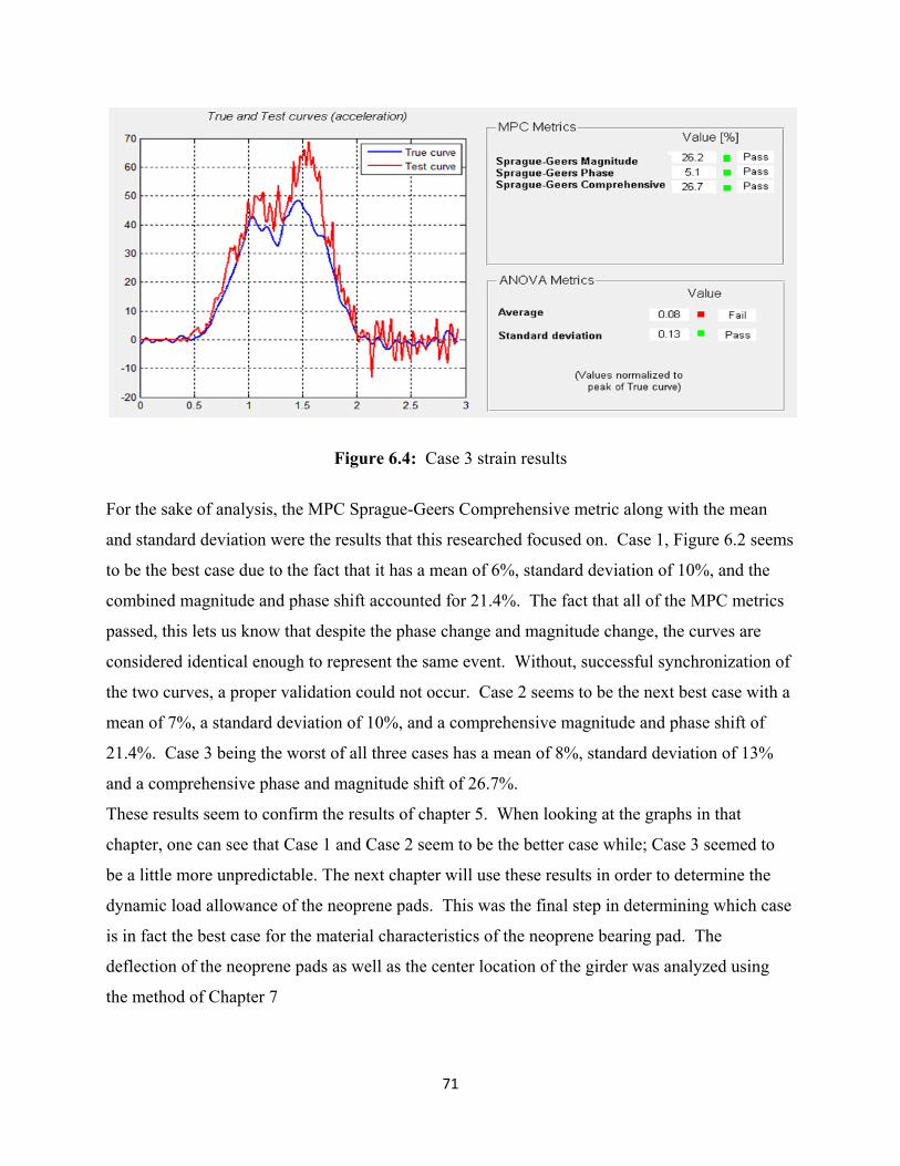
Figure 6.4: Case 3 strain results

For the sake of analysis, the MPC Sprague-Geers Comprehensive metric along with the mean

and standard deviation were the results that this researched focused on. Case 1, Figure 6.2 seems

to be the best case due to the fact that it has a mean of 6%, standard deviation of 10%, and the

combined magnitude and phase shift accounted for 21.4%. The fact that all of the MPC metrics

passed, this lets us know that despite the phase change and magnitude change, the curves are

considered identical enough to represent the same event. Without, successful synchronization of

the two curves, a proper validation could not occur. Case 2 seems to be the next best case with a

mean of 7%, a standard deviation of 10%, and a comprehensive magnitude and phase shift of

21.4%. Case 3 being the worst of all three cases has a mean of 8%, standard deviation of 13%

and a comprehensive phase and magnitude shift of 26.7%.

These results seem to confirm the results of chapter 5. When looking at the graphs in that

chapter, one can see that Case 1 and Case 2 seem to be the better case while; Case 3 seemed to

be a little more unpredictable. The next chapter will use these results in order to determine the

dynamic load allowance of the neoprene pads. This was the final step in determining which case

is in fact the best case for the material characteristics of the neoprene bearing pad. The

deflection of the neoprene pads as well as the center location of the girder was analyzed using

the method of Chapter 7

71  

CHAPTER 7

DYNAMIC LOAD ALLOWANCE FACTORS

The dynamic behavior of vehicle-bridge interaction can cause severe deterioration in the bridge,

especially in the bridge deck and in the superstructure. Since dynamic effects are significant in

the integrity of the bridge, it is necessary to consider them when evaluating an existing bridge or

designing a new one. The dynamic load allowance (DLA) is becoming more and more popular

in assessing these types of interaction.

Traditional bridge analysis has always been based on the simplifications of geometry, material,

boundary conditions and loading. With the use of dynamic load allowance factors, static

analysis can now be scaled to a more realistic result once these factors have been applied.

Currently, AASHTO has not developed an exact equation that can relate the dynamic load

allowance to the span length of the bridge but, they have an equation that can give a reasonable

approximation for determining the DLA. T using Equation 7.1. his value was calculated

    7.1 

Where L is the span length in feet. This equation actually originated from railway design but,

has been used in order to get a reasonable approximation of the DLA of highway bridges.

Another equation that was developed in the Crashworthiness and Impact Analysis Lab gives an

exact solution to determining the DLA. Unfortunately, this equation is not straight-forward and

requires the results of a dynamic analysis. a on 7.2 produces a more reliable exact solution. Equ ti

7.2

Where Rd is the dynamic response and Rs is the static response. This research utilizes Equation

7.2 due to the use of FE software is this study. Once the verification and validation of the results

were determined, they were used to calculate the DLA of the existing bridge model which was

completed in the previous research. The main reason for calculating the DLA in the existing

bridge model was to see if by improving the material and geometric properties of the neoprene

bearing pads, would there be a decrease in the dynamic load allowance. Also, whichever case

resulted in the least DLA, its pads were then implemented onto the new bridge model in order to

guarantee improvements.

72  

7.1 Evaluation of Dynamic Load Allowance

Once verification and validation is completed, the dynamic load allowance was then calculated

in regards to the displacement and strains for the entire FE bridge model. Due to the fact that the

displacement results were not validated and verified in the previous chapter, special attention

was made when calculating the total maximum displacement for each case. Equation 7.3

ensured that the neoprene pads were taken into account during the calculation process.

ΔT = ΔM + (ΔL + ΔR) 7.3

Where ΔT is the total maximum displacement, ΔM is the displacement in the middle of the girder,

ΔL is the displacement of the girders’ left neoprene pad, and ΔR is the displacement of the

girders’ right neoprene pad. Table 7.1 lists all the displacement in millimeters for each case.

Table 7.1: Total displacement values for each case

Case No. ΔM ΔL ΔR ΔT

1 -3.16 -0.478 -0.439 -3.63

2 -3.15 -0.452 -0.436 -3.59

3 -3.21 -0.598 -0.376 -3.69

By looking at Table 7.1, Case 3 deflects the most but, has the least deflection when it comes to

the center location of the girder. On the other hand, Case 3 neoprene pad deflects the most

which is what one would expect after analyzing the results of the previous chapters. Special

attention should also be made to Case 2. Earlier predictions in Chapter 5 and Chapter 6 would

have concluded that Case 1 would have the least amount of deflection but, after additional

analysis of the deflection, it is observed that in fact Case 2 has the least amount of deflection.

The result of Table 7.1 was used in order to determine the DLA for each case. Additional

analysis was performed on the strains in order to get a better idea of which case has the better

material characteristics for the improvement of the bridge model.

Unfortunately, in the previous bridge model, the displacements of the neoprene pads were not

taken into account when calculating the DLA. This resulted in total displacement values equal to

ΔM as opposed to ΔT.

73  

The next important step in calculating the DLA was to determine the static deflection for each

case now that the neoprene pads had a different shape factor and material properties. In order to

do this basic math as well as results obtained from the previous study were used. Since LS-Dyna

is a dynamic software and the static results of the previous researched utilized a field test in order

to determine the static displacement basic algebra was used to determine the static deflection for

each case. Equation 7.4 illustrates just how the static deflection was calculated in regards to the

previous research results and the current FE results.

7.4

where ΔF is the displacement obtained from the field test, ΔM is the displacement at the center of

the girder from Table 7.1, ΔT is the total displacement in Table 7.1, and ΔS is the new calculated

static displacement. Table 7.2 is a duplicate of Table 7.1 with the exception of a new colum that

displays the static deflection for all three cases.

Table 7.2: Complete displacement values

Case No. ΔM ΔL ΔR ΔS ΔT

1 -3.16 -0.478 -0.439 -3.36 -3.63

2 -3.15 -0.452 -0.436 -3.33 -3.59

3 -3.21 -0.598 -0.376 -3.35 -3.69 At first glance the static displacement seems to be larger than the dynamic displacement but,

once the total dynamic displacement is calculated one can see that it is in fact larger than the

static deflection. The shape factor is introduced again, in order to show how it affects the overall

results of the DLA factor in regards to deflection and strain. Even with a Poisson Ratio of 0.30,

which is the stiffest value that can be used for neoprene rubber, Case 1, the original case, still

seems to have a larger deflection than Case 2. These values are listed in Table 7.3.

Once the appropriate static displacements were taken into account it seems as if Case 3 is in fact

the better case. A further analysis in regards to strains was performed in order to take a closer

look at exactly which case is the best.

74  

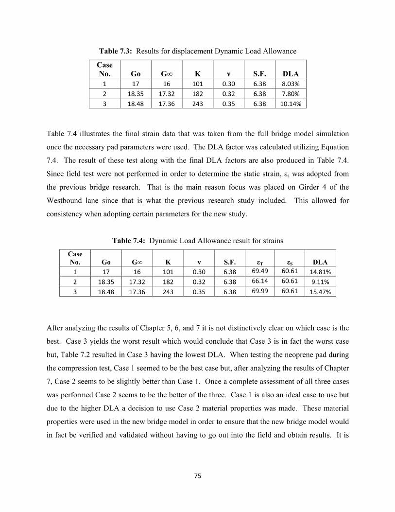
Table 7.3: Results for displacement Dynamic Load Allowance

Case

No. Go G∞ K ν S.F. DLA

1  17  16  101  0.30  6.38  8.03% 2  18.35  17.32  182  0.32  6.38  7.80% 3  18.48  17.36  243  0.35  6.38  10.14% 

Table 7.4 illustrates the final strain data that was taken from the full bridge model simulation

once the necessary pad parameters were used. The DLA factor was calculated utilizing Equation

7.4. The result of these test along with the final DLA factors are also produced in Table 7.4.

Since field test were not performed in order to determine the static strain, εs was adopted from

the previous bridge research. That is the main reason focus was placed on Girder 4 of the

Westbound lane since that is what the previous research study included. This allowed for

consistency when adopting certain parameters for the new study.

Table 7.4: Dynamic Load Allowance result for strains

Case

No. Go G∞ K ν S.F. εT εS DLA

1  17  16  101  0.30  6.38  69.49  60.61  14.81% 2  18.35  17.32  182  0.32  6.38  66.14  60.61  9.11% 3  18.48  17.36  243  0.35  6.38  69.99  60.61  15.47% 

After analyzing the results of Chapter 5, 6, and 7 it is not distinctively clear on which case is the

best. Case 3 yields the worst result which would conclude that Case 3 is in fact the worst case

but, Table 7.2 resulted in Case 3 having the lowest DLA. When testing the neoprene pad during

the compression test, Case 1 seemed to be the best case but, after analyzing the results of Chapter

7, Case 2 seems to be slightly better than Case 1. Once a complete assessment of all three cases

was performed Case 2 seems to be the better of the three. Case 1 is also an ideal case to use but

due to the higher DLA a decision to use Case 2 material properties was made. These material

properties were used in the new bridge model in order to ensure that the new bridge model would

in fact be verified and validated without having to go out into the field and obtain results. It is

75  

recommended that additional field test be done on this new bridge to ensure that the results

obtained in this study are accurate.

As a result, having a shape factor of 6.38 was vital in the improvement of the neoprene pads.

This allowed for better results without taken into account new material properties. The new

bridge model must adopt a shape factor of 6.38 in order to get better correlation with the

numerical results. Poisson Ratio also played an important role in the development of the

material properties. Despite Case 1 having the lowest shear moduli, the Poisson Ratio of 0.30

allowed for better results than Case 3 which had shear moduli of over 1 MPa higher. This

verifies the importance of this parameter in the design of elastomeric neoprene bearing pads.

This parameter seems to be as important if not more important than the shear moduli. Table 7.5

list the final geometric and material properties that should be used in the design of the neoprene

pad for the new bridge model in order to improve analytical results.

Table 7.5: Final results for improvement of neoprene pads

Case

No.

GO

(MPa)

G∞

(MPa)

K

(MPa) ν Layers

Shape

Factor

Hri

(mm)

2 18.35 17.32 182 0.32 3 6.38 12

Now that we have validated and evaluated the improvements of the neoprene pads for the

previous bridge model, verification of the new model was completed. By applying the best case,

Case 2 to the new bridge model, one can assure that the new bridge model will be verified and

partially validated due to the previous test. The results of the new bridge model are presented in

Table 7.6. Despite not having field data to completely validate the new bridge, this research

allowed for a complete verification of the results for the new bridge, No Name Creek.

Displacements are given in millimeters and strains are given as micrometers.

Table 7.6: Results for new bridge model with improved pad parameters

Case No. ΔM ΔL ΔR ΔT εT

2 -1.53 -0.509 -0.330 -1.94 69.53

76  

Now that Case 2 was chosen for improvements, a study involving different velocities was

performed on the new bridge model. In addition to the current model, four more FE analyses at

velocities of 30, 40, 60 and 70 mph were performed for the tractor-trailer located in the center of

the westbound traffic lane. These simulations allowed for estimation of the influence of the

velocity on the impact factor. The differences between the maximum deflections for the

considered velocities are relatively small however; even these slight differences had an influence

on the value of the dynamic load allowance. Equation 7.4 was utilized in order to determine the

static deflection of the AASHTO II bridge since field results were not obtained for the new

bridge model. The static deflection was calculated to be 1.75 mm and was used to determine the

DLA. The results are shown in Table 7.7 and Figure 7.1.

Table 7.7: Influence of the vehicle velocity on the dynamic load allowance

Vehicle Velocity (mph) Girder Deflection (mm) Dynamic Load Allowance (%)

0 -1.75 __

30 -1.80 2.85

40 -1.82 4.00

50 -1.89 5.02

60 -1.91 9.14

70 -1.95 11.4

0

2

4

6

8

10

12

0 20 40 60 80

DLA

 (%)

Velocity (mph)

AASHTO II

AASHTO III

Figure 7.1: Influence of the vehicle velocity on the dynamic load allowance

77  

The influence of the vehicle velocity on the DLA increases with respect to the speed. These

results verify that the AASHTO Type II model behaves in a similar matter as the previous

AASHTO Type III bridge. One can conclude by looking at these two curves that velocity does

in fact play a significant role in vehicle-bridge interaction and should be considered when

analyzing a bridge dynamic response.

7.2 Summary and Conclusion

The main purpose of this research was to develop and improve on a finite element model from an

existing bridge model. A tractor-trailer FE model was adopted from an existing project in order

to analyze vehicle-bridge interaction. Special attention was made to the neoprene bearing pads

in order to determine whether improving these pads would allow for better vehicle-bridge

interaction which ultimately would cause a lower dynamic load allowance, DLA. Since an

experimental test could not occur with the new bridge model, field results from the existing

bridge model were used in order to verify and validate improvements that were made onto the

new neoprene pads. An additional in-lab compression test FE model was created in order to

analyze the behavior of the neoprene pads once certain material parameters were discovered.

These material properties were then broken down into 3 cases in order to determine which case

would become the most successful in regards to a lower DLA thus, better vehicle-bridge

interaction. Results from the compression test were obtained and applied back onto the existing

bridge model. This was done in order to validate the improvements since field test were only

available for the existing bridge model. Once the neoprene pads were placed back onto the

bridge model successful validation between the newly improved bridge could occur. These

results were then used to calculate the new DLA in order to see whether there were

improvements made. Whichever test resulted in the lowest DLA, those material properties were

then adopted into the new bridge model that was created at the beginning of the research. This

would ensure that the new bridge model was verified through the validation of the existing

bridge model without having to do experimental test.

Initially, it was difficult to determine whether Case 1 or Case 2 was the better case. The

validation process resulted in Case 1 having the best parameters but after calculating the DLA,

Case 2 seemed to be better than Case 1. This may have to do with the fact that the DLA is based

78  

79  

solely on the maximum point as opposed to the verification method, where all points are

analyzed and an average is then calculated. After looking at the graphs of the in-lab compression

test, the results of the verification and validation program along with the DLA, Case 2 seems to

be the best case. The validation process played a major role in making the decision but, the

evaluation of the DLA was also essential when determining which case was the best. By

choosing Case 2 and applying those improvements to the new bridge model, No Name Creek, it

was assured that the results would in fact be verified but not yet validated due to lack of

experimental testing. This research in essence allowed for a complete verification of the results

of our new bridge model in regards to displacements and strains and ensured that these values

obtained in Table 7.6 would be the best results once further testing began.

7.3 Future Work

Despite improvements that were made to the neoprene pad, it is recommended that experimental

test be performed on the new bridge model to ensure the validation process and further verify the

results. Successful validation cannot occur without a set of field results. Additional parameters

such as acceleration and stress should also be analyzed. Vehicle velocity should also be

investigated further in order to make a better decision on which material parameters are the best.

In addition other vehicles should also be tested onto the bridge model such as a Terex crane and

FDOT truck to allow for further investigation of the vehicle-bridge interaction. By analyzing

multiple vehicles, one can get a better agreement on which elastomeric neoprene bearing pad

gives the lowest DLA. Once these additional parameters are analyzed, a more definitive decision

can be made in regards to which case is in fact the best.

REFERENCES

[1] AASHTO Standard Specifications for Highway Bridges (17 ed.), 2002 [2] John Roberts. What is Finite Element Analysis? Iowa State University of Science and Technology, Iowa, 2010. [3] Myint Lwin. Construction Loads on Bridges. United States Department of Transportation, Washington, DC, 2007. [4] Hongyi Li. Analytical and Experimental Evaluation of Existing Florida DOT Bridges. FAMU-FSU College of Engineering, Florida, 2004. [5] Piotr Szurgott. Investigation of Impact Factors for Permit Vehicles. FAMU-FSU College of Engineering, Florida, 2007. [6] Adam Csikos and Istvan Hegedus. Torsion of Reinforced Concrete Beams. Technical University of Budapest, Department of Reinforced Concrete Structures, Budapest, 1998. [7] Eugene J. O’Brien and Damien L. Keogh. Bridge Deck Analysis. E & FN Spon, New York, NY, 1999. [8] Stephanie Johnston, Public Works Online. Group Publisher, Chicago, IL, 2009. [9] Maupin, Brown, Lichtenstein. Extending the Life of Bridges. American Society for Testing

and Materials, Lake Buena Vista, Florida, 1990. [10] Dr. Primus Mtenga. Elastomeric Bearing Pads Under Combined Loading. FAMU-FSU College of Engineering, Tallahassee, Florida, 2006. [11] Edwards Deming. Oppurtunities are Adding up for Statisticians. American Statistical Association, Alexandria, VA, 2010. [12] Ton-Lo Wang. Influence of Heavy Trucks on Highway Bridges. Florida International University, Miami, Florida, 2000. [13] Chiara Silvestri, Marioa Mongiardini and Malcolm H. Ray. Roadside Safety Verification

and Validation Program. Worcester Polytechnic Institute, Worcestar, MA, 2009. [14] Ian Sommerville, Verification and Validation Lecture. Software Engineering, 7th Edition, 2004.

80  

[15] Charles M. Macal. Model Verification and Validation. The University of Chicago and Argonne National Laboratory, Chicago, IL, 2005. [16] Rajan Sen and Ken Spillet. Restraint Effect on Bearings. Department of Civil Engineering and Mechanics, Tampa, Florida, 1994. [17] O. Murat Hamutcuoglu and Micheal H. Scott. Finite Element Reliability Analysis of Bridge

Girders Considering Moment-Shear Interaction. Science Direct, Volume 31, Issue 5: 356-362. [18] David I. McLean, M. Lee Marsh. Dynamic Impact Factors for Bridges. Transportation Research Board National Research Council, Washington, DC, 1998. [19] Thomas J.R. Hughes, David J. Benson, and Thomas J. Lange. 11th International LS-Dyna User Conference, Livermore Software Technology, Livermore, California, 2006. [20] Marcus H. Ansley. FDOT Design Standards. Florida Department of Transportation, Tallahassee, Florida, 2006. [21] Chiara Silvestri, Marioa Mongiardini and Malcolm H. Ray. Roadside Safety Verification

and Validation Program Manuel. Worcester Polytechnic Institute, Worcestar, MA, 2009. [22] Thomas J.R. Hughes, David J. Benson, and Thomas J. Lange. 11th International LS-Dyna User Conference, Livermore Software Technology, Livermore, California, 2007. [23] ANSYS Theory Reference Manual, Structures with Material Nonlinearities 4.5, Hyperelastcity, ANSYS 7.1 Documentation, 2003. [24] Hassan Moghimi and Hamid R. Ronagh. Development of a Numerical Model for Bridge–

Vehicle Interaction and Human Response to Traffic-Induced Vibration. Elsevier Ltd., Austrailia, 2008. [25] Damon T. Allen. Stiffness Evaluation of Neoprene Bearing Pads Under Long Term Loads. University of Florida, Gainesville, Florida, 2009. [26] Abdul Aziz A. Kamal, Pauleen A. Lane and Ali A.R. Heshmati. Parametric Study of

Reinforced and Unreinforced Embankment of Soft Soil. School of Mechanical ,Aerospace and Civil Engineering, Manchester, 2005. [27] Robert Michael and David Roth. The Study of a Neoprene Elevator Roller Guide. Penn State, PA, 2003.

81  

82  

BIOGRAPHICAL SKETCH

Sharnie Earle obtained a Bachelor’s degree in Civil Engineering from the Florida State

University in 2008. Shortly after, she received her Fundamental Engineering License for the

State of Florida. She continued her education at Florida State University in order to receive her

Master of Science degree in Civil Engineering. She will begin working for Turner Construction

Company in June 2010.