Florida State University Libraries

2015

Magnetic Behavior of Heavy Elements andHeterobimetallic SystemsKariem T. Diefenbach

Follow this and additional works at the FSU Digital Library. For more information, please contact lib-ir@fsu.edu

FLORIDA STATE UNIVERSITY

COLLEGE OF ARTS AND SCIENCES

MAGNETIC BEHAVIOR OF HEAVY ELEMENTS

AND HETEROBIMETALLIC SYSTEMS

By

KARIEM T. DIEFENBACH

A Dissertation submitted to the Department of Chemistry and Biochemistry

in partial fulfillment of the requirements for the degree of

Doctor of Philosophy

2015

ii

Kariem T. Diefenbach defended this dissertation on October 13, 2015.

The members of the supervisory committee were:

Thomas E. Albrecht-Schmitt

Professor Directing Dissertation

Irinel Chiorescu

University Representative

Naresh S. Dalal

Committee Member

Joeseph B. Schlenoff

Committee Member

Oliver Steinbock

Committee Member

The Graduate School has verified and approved the above-named committee members, and

certifies that the dissertation has been approved in accordance with university requirements.

iii

To my family and all who have helped me along the way.

iv

ACKNOWLEDGMENTS

I would like to begin by thanking my parents, Thomas and Bahia, as well as my

Godparents: Kathleen, Raja, and Jan. Their never ending love and encouragement has been

invaluable. They have been a great inspiration to me through all aspects of life, teaching me how

to use heart and mind to strive for understanding. I strive to be as good a parent as they have

been to me.

To my sister, Tamara, who is full of compassion and has motivated me throughout my

life. She has the kindest soul out of any person I have ever met. Her art is unparalleled, perhaps I

am biased but she creates everything from sculptures of vicious sharks to paintings of

breathtaking scenery. She is blessed with a hardworking, patient, and considerate boyfriend,

Jason, who I am happy to call a friend.

To my girlfriend, Xue, her pragmatism, good heartedness, patience, and love have been a

blessing to me and I will cherish her forever. She has sat through many of my practice

presentations for conferences and departmental talks and soon for this dissertation’s practice as

well! She has a very analytical mind and can quickly analyze data and situations and has helped

me considerably. I have been honored to enjoy the beautiful Florida outdoors together; from

hiking and kayaking to planting gardens, a better companion I could not ask for!

To the office staff of our department who were always helpful, professional, and caring.

Particularly a truly heartfelt thank you goes to Shellie, Elizabeth, and Anna who took care of me

and all the other graduate students they were in charge of.

Dr. Schlenoff and his students took me under their wing to pursue undergraduate research

with them and continue with them until I started my graduate career. The Schlenoff group taught

me what research is all about. Ramy, who literally treated me like a brother, guided me through

v

many personal obstacles and taught me key lessons in conducting effective research. The entire

group was supportive and helped me with my research and personal life.

Sir Harry Kroto gave my entering class an introduction speech that was very uplifting,

motivating, and exciting. He taught me that even the smallest of signals, which may be mistaken

for noise, may actually yield a Nobel prize via careful experiment, patience, and dedication.

For accepting me into his lab even though I was a biochemist by training and had not

even taken a single class concerning metals or magnetism, thank you Dr. Albrecht-Schmitt. He

has an ability to teach through a historical perspective that is informative and engaging. He

taught us a large amount about some of the most amazing elements in the periodic table (again

biased I assume). A special thank you to my good friend and lab mate, Dr. Lin. He imparted a

tremendous amount of knowledge onto me, without whom I would not have learned so much so

quickly! Yilin, who will also be a life-long friend; we learned a lot from one another about life,

culture, and inorganic chemistry and my other lab mates for their friendship and knowledge.

Dr. Dalal and the gang have been incredibly helpful and fundamental to my success in

graduate school. Dr. Dalal’s deep understanding of magnetic phenomenon is fascinating. I was

lucky enough to have him as a professor during my undergraduate career and get a glimpse into

the fascinating world of quantum mechanics and especially magnetism. The group is always

available to discuss magnetic phenomenon. I am greatly appreciative to have been a part of this

wonderful group that seeks scientific knowledge with such passion.

I will stop my acknowledging people before this takes up the entire dissertation. To all

the people mentioned above and pretty much everyone I have had the pleasure of interacting

with, I am grateful and happy to have had the opportunities to work, learn, grow, and enjoy life

with.

vi

TABLE OF CONTENTS

List of Tables ............................................................................................................................... viii List of Figures ................................................................................................................................ ix Abstract ..........................................................................................................................................xv 1. INTRODUCTION ......................................................................................................................1 1.1 Introduction ..........................................................................................................................1 1.1.1 Background I: Structure and Chemistry of the f-Block Elements.............................1 1.1.2 Background II: Magnetochemistry ...........................................................................5 1.1.3 Background III: Magnetochemistry of the f-Block Elements ...................................7 2. SYNTHETIC AND EXPERIMENTAL TECHNIQUES .........................................................12 2.1 Mild Hydrothermal Synthesis ............................................................................................12 2.2 Structural Characterization Techniques .............................................................................13 2.3 Magnetic Susceptibility Measurements and Principles .....................................................14 2.3.1 Instrument Description ............................................................................................14 2.3.2 Data Acquisition......................................................................................................15 2.4 Electron Paramagnetic Resonance .....................................................................................16 2.4.1 X-Band and Q-Band Instrument Description ..........................................................16 2.4.2 High-Frequency EPR Instrument Description ........................................................17 2.4.3 Principles .................................................................................................................18 2.4.4 Data Acquisition......................................................................................................19 3. STRUCTURE AND MAGNETIC PROPERTIES OF NEPTUNIUM SELENITES ..............21 3.1 Introduction ........................................................................................................................21 3.2 Experimental Descriptions of Np(SeO3)2 and NpO2(SeO3)...............................................23 3.2.1 Synthesis of Np(SeO3)2 and NpO2(SeO3) ...............................................................23 3.2.2 Magnetic Susceptibility Measurements ..................................................................24 3.3 Crystal Structure Analysis .................................................................................................25 3.3.1 Structure of Np(SeO3)2 ............................................................................................25 3.3.2 Structure of NpO2(SeO3) .........................................................................................25 3.4 Magnetic Studies ................................................................................................................28 3.5 UV-vis-NIR Spectroscopy .................................................................................................29 3.6 Conclusions .......................................................................................................................31 4. SPIN GLASS AND LONG RANGE FERROMAGNETIC ORDERING EXHIBITED BY NEPTUNIUM IODATES ..............................................................................................................33 4.1 Introduction ........................................................................................................................33 4.2 Synthesis and Experimental Descriptions ..........................................................................34 4.2.1 Synthesis of NpO2(IO3)(H2O)•H2O ........................................................................34

vii

4.2.2 Synthesis of NpO2(IO3) ...........................................................................................35 4.2.3 Magnetic Susceptibility Measurements ..................................................................35 4.3 Crystal Structure Analysis .................................................................................................36 4.4 Magnetic Studies ................................................................................................................37 4.5 Conclusions .......................................................................................................................44 5. STRUCTURE-PROPERTY RELATIONSHIPS IN LANTHANIDE COPPER SULFATE HETEROBIMETALLIC COMPOUNDS .....................................................................................46 5.1 Introduction ........................................................................................................................46 5.2 Synthesis and Experimental Descriptions ..........................................................................48 5.3 Structural Descriptions.......................................................................................................49 5.4 Periodic Trends ..................................................................................................................54 5.5 Analysis of Magnetic Susceptibility and Magnetization ...................................................55 5.6 Electron Paramagnetic Resonance .....................................................................................61 5.7 Conclusions .......................................................................................................................64 6. MAGNETIC PROPERTIES OF VARIOUS OTHER SYSTEMS ...........................................66 6.1 Introduction ........................................................................................................................66 6.2 Cs6U3Sb2P8S32: A Spin Frustrated System ........................................................................68 6.3 Magnetic Properties of Lanthanide-Transition Metal Heterobimetallic Compounds........70 6.3.1 Synthesis and Structure ...........................................................................................71 6.3.2 Magnetic Behavior of Ln2Cu(TeO3)2(SO4)2 ...........................................................73 6.3.3 Magnetic Behavior of Ln2Co(TeO3)2(SO4)2 and Ln2Zn(TeO3)2(SO4)2 ..................80 6.4. Antiferromagnetic Ordering in Cu3(TeO4)(SO4)•H2O .......................................................89 6.5 Conclusions .......................................................................................................................96 7. SUMMARY AND ANALYSIS ................................................................................................98 APPENDIX ..................................................................................................................................100 A. COPYRIGHT INFORMATION .............................................................................................100 BIBLIOGRAPHY ........................................................................................................................104 BIOGRAPHICAL SKETCH .......................................................................................................111

viii

LIST OF TABLES

Table 1.1 Formal oxidation states across the actinide series (bold and highlighted are the most stable, parentheses indicate low stability, and in red with italics indicates possibly viable states). 3 Table 1.2 Russel-Saunders term symbols, effective magnetic moments, and other theoretical magnetic constants for the +3 formal oxidation states of the lanthanide series, Ln3+ ions.24 ........10 Table 3.1 Selected crystallographic data for Np(SeO3)2 and NpO2(SeO3) ....................................27

Table 4.1 Selected crystallographic data for the structure NpO2(IO3)H2O•H2O. ..........................36 Table 4.2 Selected bond distances surrounding the neptunium and iodine nuclei within the structure of NpO2(IO3)(H2O)•H2O .................................................................................................39 Table 6.1 The closest Ln3+

···Ln3+, Ln3+···Co2+, and Co2+

···Co2+ bond distances in Ln2Co(TeO3)2(SO4)2 are shown for each of the measured lanthanides .........................................81

ix

LIST OF FIGURES

Figure 1.1 Using density functional theory, Jeffrey Hay and Richard Martin of Los Alamos calculated the radial distribution functions for an isolated Sm3+ ion showing the various orbital probability densities as a function of radial distribution. The relativistic(solid line) and nonrelativistic(dashed line) calculations are shown.18 Adapted from Crosswhite et al, J. Chem.

Phys., 1980, 72 (9), 5103-5117. .......................................................................................................5

Figure 1.2 Using density functional theory, Jeffrey Hay and Richard Martin of Los Alamos calculated the radial distribution functions for an isolated Pu3+ ion showing the various orbital probability densities as a function of radial distribution. The relativistic (solid line) and nonrelativistic (dashed line) calculations are shown.20 Adapted from Crosswhite et al, J. Chem.

Phys., 1980, 72 (9), 5103-5117. .......................................................................................................6

Figure 1.3 Magnetic susceptibility as a funciton of temperature showing the expected behavior for a ferromagnetic (blue) paramagnetic (black) and antiferromagnetic(pink) material with their respective transition points. Adapted from https://en.wikipedia.org/wiki/Magnetochemistry ........7 Figure 1.4 The calculated (solid line) and experimental (large data points) magnetic moments are shown for the Ln3+ ions across the series. These results show that angular momentum must be accounted for. The experimental data matches closely with the calculated J states rather than the spin only moment, indicating strong spin-orbit coupling.23 Adapted from Buschow, K. H. J.; De Boer, F. R., Physics of Magnetism and Magnetic Materials, 2012. ................................................9 Figure 2.1 A dismantled hydrothermal reaction vessel with the stainless steel jacket on the left and a Teflon® liner shown on the right, between the two are the anti-rupture components. ........13 Figure 2.2 The Quantum Design magnetic property measurement system, MPMS, used for magnetic susceptability measurements is shown. The noteworthy components are labeled within the figure and the evercool is an added recycler used to recycle the liquid helium. .....................15 Figure 2.3 Bruker Elexsys E500 EPR Spectrometer and its various components are shown including the temperature control unit, “Liquid N2 Temperature Control.” The liquid nitrogen would flow from a Dewar behind the electromagnet to cool the sample. .....................................17 Figure 2.4 An energy level scheme is depicted for a simple one electron system with an applied magnetic field. The resonance condition is achieved once the energy, or incoming radiation, is equivalent to .....................................................................................................................19 Figure 3.1 (a) View along the a axis of part of the structure of Np(SeO3)2. (b) Chain of edge-sharing NpO8 units extending along the a axis. Neptunium-containing polyhedra are shown in drab, the selenite units in light green. (c) Layers of NpO2(SeO3) stacking along the c axis. (d) View of a NpO2(SeO3) layer in the [ab] plane. Neptunium polyhedra are shown in garnet, the selenite structural units in light green ............................................................................................26

x

Figure 3.2 Coordination environments of the neptunium centers: (a) The eight-coordinate Np4+site in Np(SeO3)2 is best described as a bicapped trigonal prism. (b) The Np6+site in NpO2(SeO3) has a hexagonal bipyramidal geometry .....................................................................28 Figure 3.3 Magnetic properties of Np(SeO3)2: (a) The temperature dependence of zero-field-cooled (ZFC) and field-cooled (FC) DC magnetic susceptibility measured at 100 Oe. Inset: the temperature dependence of 1/ showing the large temperature-independent paramagnetic contribution. (b) The temperature dependence of AC magnetic susceptibility measured at various frequencies of the applied AC field and zero DC bias field. (c) Isothermal field dependence of magnetization measured at 1.8 K ...................................................................................................30 Figure 3.4 UV-vis-NIR spectra of Np(SeO3)2 and NpO2(SeO3) at 298 K along with an image of the crystal that was analyzed..........................................................................................................32

Figure 4.1 (a) View along the c axis of part of the structure of NpO2(IO3)(H2O)•H2O exhibiting the cation-cation interactions of the NpO7 units which are in green with oxygen atoms shown in red. (b) Layers of corner-sharing NpO7 units extending along the a axis. Neptunium-containing polyhedra are shown in green, oxygen atoms that are part of water molecules are in blue while the rest of the oxygen atoms are red. Iodate anions are purple .....................................................38 Figure 4.2 The magnetic susceptibility for (a) NpO2(IO3)(H2O)• H2O and (b) NpO2(IO3) measured under an applied magnetic field of 400 Oe using zero field cooled (red) and field cooled (black). The insets show the inverse susceptibility as a function of temperature. .............40 Figure 4.3 The zero field cooled magnetic susceptibilities for NpO2(IO3) and NpO2(IO3)(H2O)•(H2O) measured under a field of 100 Oe. The dashed blue line represents the mean-field ordering model .............................................................................................................41 Figure 4.4 The isothermal field dependence of (a) NpO2(IO3)(H2O)•H2O and (b) NpO2(IO3) measured at 1.8 K. The insets display the magnetic hysteresis near 0 applied magnetic field, highlighting the slight amount of remnant magnetization and coercivity .....................................42 Figure 4.5 The real component of the alternating current magnetic susceptibility is plotted for (a) NpO2(IO3)(H2O)•H2O and (d) NpO2(IO3). The imaginary components, χ”, of the AC magnetic susceptibility for (b) NpO2(IO3)(H2O)•H2O and (e) NpO2(IO3). The various colors and shapes represent the different frequencies of the driving field as detailed in the legend. Finally, the Arrhenius fittings to the plots of the imaginary component are shown in (c) NpO2(IO3)(H2O)•H2O and (f) NpO2(IO3) ......................................................................................43 Figure 5.1 Crystal images of LnCuSO4-1 (Sm, Eu, Gd, Dy, and Ho), LnCuSO4-2 (Ln = Tm, Yb, and Lu), LnCuSO4-3 (Ln = Nd, Sm, Eu, and Gd), and LnCuSO4-4 (Ln = Dy, Ho, Er, Tm, Yb, and Lu) ...........................................................................................................................................50 Figure 5.2 View of the structures of (a) LnCuSO4-1 (Sm, Eu, Gd, Dy, and Ho), (b) LnCuSO4-2 (Ln = Tm, Yb, and Lu), (c) LnCuSO4-3 (Ln = Nd, Sm, Eu, and Gd), and (d) LnCuSO4-4 (Ln = Dy, Ho, Er, Tm, Yb, and Lu). Lanthanide polyhedra are shown in dark blue, pink, cyan, and

xi

purple in LnCuSO4-1, LnCuSO4-2, LnCuSO4-3, and LnCuSO4-4, respectively. Copper ions are shown in dark blue with sulfate tetrahedra in gray ........................................................................51 Figure 5.3 Structures of (a) LnCuSO4-1 (Sm, Eu, Gd, Dy, and Ho), (b) LnCuSO4-2 (Ln = Tm, Yb, and Lu), (c) LnCuSO4-3 (Ln = Nd, Sm, Eu, and Gd), and (d) LnCuSO4-4 (Ln = Dy, Ho, Er, Tm, Yb, and Lu). These structures emphasize the connectivities of Ln polyhedra bridged by oxygen atoms. Lanthanide ions are shown in dark blue, pink, cyan, and purple in LnCuSO4-1, LnCuSO4-2, LnCuSO4-3, and LnCuSO4-4, respectively. Oxygen atoms are in red .....................52 Figure 5.4 Representation of the coordination geometries of lanthanide ions in (a) LnCuSO4-1 (Sm, Eu, Gd, Dy, and Ho), (b) LnCuSO4-2 (Ln = Tm, Yb, and Lu), (c) LnCuSO4-3 (Ln = Ln = Nd, Sm, Eu, and Gd), and (d) LnCuSO4-4 (Ln = Dy, Ho, Er, Tm, Yb, and Lu) ..........................54 Figure 5.5 Plots of the inverse of the ionic radii versus the number of the f electrons for (a) LnCuSO4-1 (Sm, Eu, Gd, Dy, and Ho) and LnCuSO4-2 (Ln = Tm, Yb, and Lu); (b) LnCuSO4-3 (Ln = Ln = Nd, Sm, Eu, and Gd) and LnCuSO4-4 (Ln = Dy, Ho, Er, Tm, Yb, and Lu) ..............56 Figure 5.6 Temperature dependence of (a) , (b) –1, and (c) field dependence of magnetization at 1.8 K for GdCuSO4-1.The solid line in (b) represents a fit to the Curie-Weiss law. The solid curve in (c) represents the simulated Brillouin function assuming paramagnetic interactions .....................................................................................................................................58 Figure 5.7 Temperature dependence of (a) , (b) T with –1 inset, and (c) field dependence of magnetization at 1.8 K for GdCuSO4-3. In (c), the solid curve represents the simulated Brillouin function assuming paramagnetic interactions with an inset of the near zero hysteresis ................59 Figure 5.8 Temperature dependence of (a) with an inset of –1, (b) T, and (c) field dependence of magnetization at 1.8 K for YbCuSO4-2. In (c), the solid curve represents the simulated Brillouin function assuming paramagnetic interactions while the solid line represents a linear fit in that regime ...................................................................................................................60 Figure 5.9 Temperature dependence of (a) , (b) –1 with a solid line fit to the Curie-Weiss law, and (c) field dependence of magnetization at 1.8 K for YbCuSO4-4. In (c), the solid curve represents the simulated Brillouin function assuming paramagnetic interactions .........................61 Figure 5.10 Temperature dependence of (a) , (b) T, (c) field dependent magnetization for HoCuSO4-4 with the solid curve represents the simulated Brillouin function assuming paramagnetic interactions while the solid line represents a linear fit in that regime .....................61 Figure 5.11 The EPR spectra of Gd2Cu(SO4)2(OH)4 (in black, GdCuSO4-1) and GdCu(SO4)(OH)3 (in green, GdCuSO4-3). Data were acquired at room temperature using a 34 GHz source. The differences in the line shapes clarrify the differences in magnetic behavior .....62 Figure 5.12 EPR spectra and simulations preformed on (a) GdCuSO4-1 and (b) GdCuSO4-3 at room temperature using 34 GHz, Q band measurements ..............................................................63

xii

Figure 5.13 High frequency high field EPR spectra of (a) GdCuSO4-1 measured at 50 K and 5 K and (b) GdCuSO4-3 measured at 50 K, 15 K, and 5 K ..................................................................64 Figure 5.14 Peak to peak linewidths of GdCuSO4-3 as a function of temperature. The maximum peak to peak linewidth occurs near 75 K due to the splitting of the isotropic g tensor .................65 Figure 6.1 The U4+ ions are shown by the green spheres while antimony and sulfur are

represented in red and yellow, respectively. The [U3S18]24− trimers are capped by two [PS4]

3−

units that are connected via [Sb(PS4)3]6− anions ............................................................................69

Figure 6.2 Temperature dependence of the inverse magnetic susceptibility, 1/χ, of Cs6U3Sb2P8S20 is shown. The solid blue line represents the fitting to the Curie-Weiss law. Zero field cooled measurements were conducted under an applied field of 0.1 T. The blue line shows the fit in the range of 75 to 150 K to the Curie-Weiss law.................................................................................70 Figure 6.3 Field dependent Magnetization of Cs6U3Sb2P8S20 obtained at 1.8 K with an applied magnetic field ranging from 0 Oe up to 70 000 Oe .......................................................................71 Figure 6.4 (a) View of the structure of Ln2TM(TeO3)2(SO4)2 (RE = Y, Nd, Sm, Eu, Gd, Tb, Dy, Ho, Er, or Tm. TM = Co, Zn, or Cu) extending down the a axis. (b) Representation of the trigonal dodecahedron coordination environment of Ln3+ ions. (c) [TM(TeO3)2(SO4)2]

6- unit. Ln3+ polyhedra are shown in cyan, TM2+ polyhedra in dark blue, TeO3

2- polyhedra in grey, SO42-

tetrahedra in purple, and oxygen atoms in red ...............................................................................72 Figure 6.5 (a) Structural view of Ln2TM(TeO3)2(SO4)2 (Ln = Yb or Lu and TM = Cu, Co, or Zn) extending down the a axis. (b) Representation of the pentagonal bipyramid coordination environment of RE3+. (c) [TM(TeO3)2(SO4)2]

6- unit. RE3+ polyhedra are shown in green, TM2+ polyhedra in dark blue, TeO3

2- polyhedra in grey, SO42- tetrahedra in purple, and oxygen atoms

in red ..............................................................................................................................................73 Figure 6.6 Photographs of crystals of Ln2Co(TeO3)2(SO4)2. From left to right and top to bottom can be seen the following analogues: Ln = Y, Nd, Sm, Eu, Gd, Tb, Dy, Ho, Er, Tm, Yb, and Lu. ..................................................................................................................................................74 Figure 6.7 Temperature dependence of magnetic susceptibility (a), inverse susceptibility (inset), and the T product (b) for Y2Cu(TeO3)2(SO4)2. (c) Field-dependent magnetization measured at 1.8 K. The solid red line in (a) shows the theoretical fit to the modified Curie-Weiss law. .................................................................................................................................................75 Figure 6.8 Temperature dependence of T (a and b), (c and d), and field dependence of magnetization at 1.8 K (e and f) for Sm2Cu(TeO3)2(SO4)2 and Eu2Cu(TeO3)2(SO4)2, respectively ...................................................................................................................................76

xiii

Figure 6.9 Temperature dependence of T (a) and –1 (inset) and the field dependence of magnetization at 1.8 K (b) for Dy2Cu(TeO3)2(SO4)2. The solid red line in (a) shows the fit to the modified Curie-Weiss law, while the solid black line in (b) represents the magnetization calculated as the sum of Brillouin functions for two Dy3+ and one Cu2+ ions ...............................78 Figure 6.10 Temperature dependence of T and 1.8-K field dependence of magnetization (insets) for Ln2Cu(TeO3)2(SO4)2, where Ln = Gd (a), Ho (b), Er (c), and Tm (d). The solid lines in the insets represent the magnetization calculated as the sum of Brillouin functions for two Ln3+ and one Cu2+ ions ..................................................................................................................................79 Figure 6.11 Temperature dependence of T and 1.8-K field dependence of magnetization (inset) for Yb2Cu(TeO3)2(SO4)2. The solid line represents the magnetization calculated as the sum of Brillouin functions for two Ln3+ and one Cu2+ ions .......................................................................80 Figure 6.12 Temperature dependence of magnetic susceptibility , T product with inverse susceptibility as an inset for Y2Co(TeO3)2(SO4)2 (a, b), Eu2Co(TeO3)2(SO4)2 (c, d), and Lu2Co(TeO3)2(SO4)2 (e, f). The solid red lines in the insets show the fitting to the Curie-Weiss law in terms of inverse susceptibility .............................................................................................83 Figure 6.13 Temperature dependence of magnetic (a) magnetic susceptibility, , inverse magnetic susceptibility (inset), and the (b) T product for Nd2Co(TeO3)2(SO4)2 .........................84 Figure 6.14 Temperature dependence of magnetic susceptibility , inverse susceptibility (inset), and the T product for (a,b) Gd2Co(TeO3)2(SO4)2, (c,d) Tb2Co(TeO3)2(SO4)2, (e,f) Dy2Co(TeO3)2(SO4)2 ......................................................................................................................85 Figure 6.15 Temperature dependence of magnetic susceptibility, , inverse susceptibility (inset), and the T product for (a,b) Ho2Co(TeO3)2(SO4)2 and Ho2Zn(TeO3)2(SO4)2. (c,d) Er2Co(TeO3)2(SO4)2 and Er2Zn(TeO3)2(SO4)2 ...............................................................................87 Figure 6.16 (a) Temperature dependence of magnetic susceptibility, , inverse susceptibility, -1, (inset), and (b)the T product for Yb2Co(TeO3)2(SO4)2 ................................................................88 Figure 6.17 Magnetization plots of (a) Y2Co(TeO3)2(SO4)2, (b) Gd2Co(TeO3)2(SO4)2, (c) Tb2Co(TeO3)2(SO4)2, (d) Dy2Co(TeO3)2(SO4)2. The solid red line represents the theoretical Brillouin fitting which accounts for non-interacting magnetic spins with spin orbit coupling .....90 Figure 6.18 (a) View of the structure of Cu3(TeO4)(SO4)·H2O down the b axis; (b) View of the structure of Cu3(TeO4)(SO4)·H2O down the c axis. Copper polyhedra are shown in green, tellurite polyhedra in cyan, and sulfate anions in grey ..................................................................91 Figure 6.19 (a) Temperature dependence of magnetic susceptibility χ at 1000 Oe and 100 Oe (inset) for Cu3(TeO3)(SO4)(H2O)2; (b) field dependence of magnetization at 1.8 K, 50 K, 70 K, and 80 K for Cu3(TeO3)(SO4)(H2O)2, (c) A ball and stick model of the Cu2+ ions showing the Cu(1) ions in light green and the Cu(2) ions in dark green. ..........................................................92

xiv

Figure 6.20 This EPR spectrum was performed at room temperature, X band, on a powdered sample of Cu3(TeO4)(SO4)·H2O. This spectrum does not distinguish between the three Cu2+ ions and assigns them axial symmetry ..................................................................................................93 Figure 6.21 This figure shows the Q band EPR spectra of powdered Cu3(TeO4)(SO4)·H2O. All three Cu2+ ions have similar local symmetry, distorted square planar, such that the three principal magnetic axes are distinctly different. The value of 2.089 corresponds to the out of plane orientation, with dz

2 as the ground state .........................................................................................94

Figure 6.22 HFEPR spectra are shown for powdered Cu3(TeO4)(SO4)·H2O at room temperature and 5 K using 240 GHz. Peaks are labeled from right to left with a vertical dashed blue line showing the peak shift over the measured temperature range. The black and red values represent the corresponding g tensors for the respective peaks .....................................................................95

xv

ABSTRACT

The focus of this dissertation is the study of the magnetic properties of several novel

lanthanide and actinide metal complexes, of particular concentration is the use of SQUID

magnetochemistry coupled with electron paramagnetic resonance (EPR). Through these

techniques, a deeper understanding of the magnetic behavior of the f elements and their

structure-property relationships are realized.

The novel neptunium selenite compounds presented in Chapter 3 are simple systems in

which to probe the magnetic susceptibilities of transuranic compounds and a soft ferromagnetic

material with strong temperature independent paramagnetic effects was synthesized.

Chapter 4 also concerns neptunium but in this case a comparison between neptunium

iodates, which are expected to be nonmagnetic, assuming a formal oxidation state of +5 which

yields a singlet ground (S = 1) assuming spin only contributions. The compounds actually

display ferromagnetic ordering at approximately 12 K. Of even further interest is the frequency

dependence of the magnetic susceptibility which should not be evident in a magnetically ordered

system thus signifying the material have spin glass properties or exhibit magnetic frustrations.

The focus of Chapter 5 is the correlations between structure and magnetic properties that

are correlated in a large family of heterobimetallic compounds containing lanthanides and

copper. The tuning of the magnetic properties can be controlled by careful substitution of

lanthanide ions. Of particular interest is the magnetic information revealed via electron

paramagnetic resonance which may go unnoticed by bulk magnetization techniques. These

measurements clarified the magnetic description of the compounds.

Chapter 6 highlights several other compounds that were found to be magnetically

interesting. Particularly interesting is a uranium ion in the +4 oxidation state that exhibits spin

xvi

frustration. Furthermore, a large family of lanthanide-transition metal ions with tellurium and

sulfate anions, where both the lanthanides and transition metal ions are able to be substituted

yielded a large diversity of magnetic properties. Finally, a compound was synthesized that

exhibited two crystallographically unique copper atoms which are distinguishable via high field

electron paramagnetic resonance and order antiferromagnetically.

1

CHAPTER 1

INTRODUCTION

1.1 Introduction

Life in the twenty-first century hinges on the manipulation of electronic and magnetic

properties of materials. Valence electrons are what control these properties and the

understanding of these minute particles gives rise to our technological civilization. These

magnetic properties are intrinsic to everything; whether they are observed in refrigerator

magnets and iron fillings or imperceptible such as in a copy of a dissertation or a chair. The

probing of valence electrons is necessary to better understand novel materials and thus design

materials for specific uses.

Being interested in this field is only natural as it plays such a central role in our daily

lives from keeping track of currency to typing this dissertation. Growing up in the vicinity of

one of the greatest places in the world to study magnetism, what was known as the National

High Magnetic Field Laboratory (Mag Lab), furthered my interest in pursuing this research

subject. Every once in a while the Mag Lab hosts an open house where they demonstrate a

wide variety of fantastic experiments that are fantastic and eye opening to the young mind.

Attending these open houses as a boy inspired me at a young age to learn more.

In the next few subsections a background into the structure and chemistry of the rare

earths and actinides are presented as well as magnetochesmitry and specifically how it

pertains to these heavier elements.

1.1.1 Background I: Structure and Chemistry of the f-Block Elements

Comprising about a fourth of the periodic table, one would think that f-block

chemistry would be well understood but their relativly recent discoveries and isolation is an

2

attributor to their under exploration. The actinides in particular have not been widely studied

due primarily to radiological safety issues and very small quantities, especially the later

actinides. Though many of our technologies rely on lanthanide materials, actinides have the

potential to give rise to novel technologies or enhance the performance of existing ones.

Thus, it is important to study the similarities and differences between these two f- block

series.1, 2 For instance, the 4f series is most stable in the trivalent oxidation state while the

early actinides have a wide variety of stable oxidation states, commonly trivalent to

heptavalent (Table 1.1).2, 3 The variabliltiy of oxidation state exhibited by the earliy actinides

is similarly observed in transition metals. The later actinides favor the trivalent state and are

assumed to behave more like the lanthanides. Plutonium resides between the early actinides

and the core-like later actinides and it is arguably the most complex element on the periodic

table especially due to its easy variablility of oxidation states and allotropes. In solution,

plutonium exhibits formal oxidation states between +3 and +6, as the standard reduction

potential between each of these species is approximately 1 V.2 As plutonium is heated, it

undergoes seven phase transitions which changes crystal structure, maleability, density, and

various other properties.4 On the other hand, neptunium, nestled between uranium and

plutonium on the periodic table, has been relativly neglected with only about 1/17 the crystal

structures as its neighbors based on the Cambridge Structural Database and Inorganic Crystal

Structural Database as of August 2015. The wide range of oxidation states exhibited by

neptunium lends itself to a wide variety of exesible chemistry.1, 2 The Np5+ species is the

major participant in this chemistry due in part to the stability of this state with respect to

disproportionation.5-7 Moreover, neptunium in the penta- and hexavalent states adopts highly

anisotropic coordination geometries, primarily because of the tendency for forming the linear

3

dioxo neptunyl ions, NpO2n+ (n = 1 or 2). These moieties are further coordinated by four to

six additional donor atoms in a plane perpendicular to the neptunyl axis yielding tetragonal,

pentagonal, and hexagonal bipyramidal environments around the neptunium centers.8, 9 The

geometries exhibited by the tri- and tetravalent oxidation states are substantially different

from the aforementioned ones, and these ions are typically found in eight- and nine-

coordinate environments with a variety of distortions of dodecahedra (CN = 8) and tricapped

trigonal prisms (CN = 9).10-12 The eight-coordinate neptunium centers are particularly

complex because cubic (Oh),13 trigonal dodecahedral (D2d),

10 bicapped trigonal prismatic

(C2v),14

and square antiprismatic (D4d)10 all occur. Neptunium’s ability to comproprtionate

into the formal +5 oxidation state and readily disproportionate into the +4 and +6 oxidation

states yields several interesting compounds from single reactions as shown in Chapter 3 and

Chapter 4 of this dissertation.

Actinide Ac Th Pa U Np Pu Am Cm Bk Cf Es Fm Md No Lr

Formal

Oxidation

States

1

(2) (2) (2) (2) 2 2 2 2

3 (3) (3) 3 3 3 3 3 3 3 3 3 3 3 3

4 4 4 4 4 4 4 4 4 4

5 5 5 5 5 5 5

6 6 6 6 6

7 7 7

8

In addition, going across the lanthanide series, a slight and constant decrease in the

radial extension of the atoms known as the lanthanide contraction is evidenced.15 The

contraction arises due to poor shielding by the 4f electrons which do not increase

proportionatly with the nuclear charge forcing the valence electrons towards the nucleus.16

Table 1.1 Formal oxidation states across the actinide series (bold and highlighted are the most stable, paranthases indicate low stability, and in red with italics indicates possibly viable states).

4

This contraction is the primary reason that it is possible to separate the lanthanides from one

another. A similar effect is observed in the actide series although relativistic effects play a

larger role. Furthermore, the lanthanide contraction also causes the 5d elements to have

similar chesmitry to the 4d transition metals.

Another major difference between lanthanides and actinides is bonding, in particular

covalence; the lanthanides tend to have ionic natured interactions due to the core like 4f

orbitals while the actinides exhibit more covalent like bonding.17 The more core like 4f

orbitals do not interact with ligand orbitals due to their radial extension not overlaping typical

bond lengths. Figure 1.1 shows the calculated radial extension for Sm3+ as an example of

how limited the 4f orbital’s radial extension is and the electron density dimineshes quickly

after 1 Å.18 The limited interactions between 4f orbitals and ligands is clearly seen by the

ligand independant sharp f-f transitions observed via spectroscopic techniques.

The calculations for actinide radial distribution for orbitals is slightly different than

for the lanthanides (Figure 1.2). The 5f orbitals extend farther than the 4f, overlaping with

other orbitals. A clear comparison can be seen by examining the probability density of

finding an electron at 1 Å, for the actinides the probility of an 5f electron is 4 times greater

than for the 4f lanthanides.

Valence actinide electrons exhibit contributions from a mix of orbitals, 5f-6d-7s,

which are close in energy and form the conduction band. Due to contributions from the more

diffuse 7s, 6d, and even the 7p orbitals, the actinides have a farther orbital radial extension

than their lanthanide counterparts which overlap with ligand orbitals resulting in more

covalent character.19 Thus by quantifying the orbital overlap and mixing coeffecients, the

amount of covalency can be determined.20

5

1.1.2 Background II: Magnetochemistry

There are two major types of magnetic behavior that can be used to classify all

materials, they either have unpaired electrons or all be paired. The latter is termed

Diamagnetic and slightly repels an applied external magnetic field. Nearly all elements have

paired electrons and thus have a diamagnetic contribution. Compounds with unpaired

electrons are attracted to magnetic fields and are termed paramagnetic. Paramagnetic

materials can undergo phase transitions where the unpaired electrons are effected by one

another and an external magnetic field. If unpaired electrons spontaneously allign with one

Figure 1.1 Using density functional theory, Jeffrey Hay and Richard Martin of Los Alamos calculated the radial distribution functions for an isolated Sm3+ ion showing the various orbital probability densities as a function of radial distribution. The relativistic(solid line) and nonrelativistic(dashed line) calculations are shown.18 Adapted from Crosswhite et al, J.

Chem. Phys., 1980, 72 (9), 5103-5117.

6

another, they are classified as ferromagnetic and form domains with varying sizes based on

the strength of the applied field.

The temperature at which the magnetic moments aligh is the critcal temperature and

is called Curie point, TC. The unpaired electrons can also become paired with one another at a

certain temperature, the Néel point, defining the material as antiferromagnetic. Figure 1.3

demonstrates the magnetic susceptibility of such magnetic transitions as a function of

temperature. Another type of subdivision to paramagnetic materials is ferrimagnetic where

the spins allign anti-parallel to one another but the relative strengths of the pairings are

unequal yielding a net moment.

Figure 1.2 Using density functional theory, Jeffrey Hay and Richard Martin of Los Alamos calculated the radial distribution functions for an isolated Pu3+ ion showing the various orbital probability densities as a function of radial distribution. The relativistic (solid line) and nonrelativistic (dashed line) calculations are shown.20 Adapted from Crosswhite et al, J.

Chem. Phys., 1980, 72 (9), 5103-5117.

7

1.1.3 Background III: Magnetochemistry of the f-Block Elements

Known as the strongest permanent magnets, SmCo5 and Nd2Fe14B, were discovered

in the early 1970s and 1980s, respectively. These two magnets are known to have

extraordinary properties, which are due in part to 3d-4f magnetic exchange.21 Our study of

novel materials with various 3d-4f magnetic exchange have resulted in a wide variety of

compounds with various magnetic and physicochemical properties.22

The magnetochemistry of 3d transition metal chemistry can usually be approximated

by the unpaired electrons, or total spin of the system, S, with the other contributions being

mearly pertubations. This differs from the heavier f-block magnetochesmitry in that what

Figure 1.3 Magnetic susceptibility as a funciton of temperature showing the expected behavior for a ferromagnetic (blue) paramagnetic (black) and antiferromagnetic(pink) material with their respective transition points. Adapted from https://en.wikipedia.org/wiki/Magnetochemistry

8

was previously a pertubation is now a major contributing affect. One such example is

orbital angular momentum, L, and it’s coupling with the spin magnetic moment, which

results in the total angular momentum, J, being a more valid quantum number. The total spin

moment must be subtracted from the angular momentum when the f shells are less than half

filled and added when the shell is more than half filled yielding the total angular momentum

of the magnetic ion. This is termed spin-orbit coupling and is demonstrated in Figure 1.4 by

comparing experimental and calculated results of various trivalent lanthanides.

Spin-orbit effects are just the first step in understanding the magnetic behavior of the

heavy elements and complexes thereof. These effects are of greater prominence as the

nuclear charge is increased. The Russel-Saunders coupling scheme (R-S) uses Hund’s rules

to determine the ground state of an ion, assigning it a R-S term symbol. Table 1.2 displays

the R-S terms symbols as well as other terms symbols and theoretical values. In particular,

for actinide magnetochemistry the R-S excited J states can mix with the ground state due to

easily exessible energy levels which complicates the ground state. The mixing of J states is

considered in intermediate-coupling, resulting from spin-spin repulsions, spin-orbit coupling,

and crystal field splittings, which invalidates S and L as good quantum numbers. Another

coupling scheme is j-j coupling which combines the total angular momentum for each ion

instead of summing the total spin and angular contributions which more accuratly captures

the orbital contributions than the R-S coupling for the f-block elements.

Overall, intermediate-coupling gives the most accurate representation of experimental

results but it is calculation intensive as compared to the R-S and j-j coupling schemes which

yield very close and experimentaly valid approximations.

9

Crystal field effects are another key contributor to lanthanide and actinide

magnetochemistry which remove the degeneracy of the ground state into 2J+1 sublevels, mJ,

based on the ligand symmetry surrounding the magnetic ion.

These effects are nearly negligable, but play a major role in molecular systems of

these heavy elements due to energetically similar sublevels.

Figure 1.4 The calculated (solid line) and experimental (large data points) magnetic moments are shown for the Ln3+ ions across the series. These results show that angular momentum must be accounted for. The experimental data matches closely with the calculated J states rather than the spin only moment, indicating strong spin-orbit coupling.23 Adapted from Buschow, K. H. J.; De Boer, F. R., Physics of Magnetism and Magnetic Materials, 2012.

10

Ion 4f n Groun

d State S L J G g J(J 1) gJ

La3+ 0 1S0 0 0 0 0 0 0

Ce3+ 1 2F5/2 1/2 3 5/2 6/7 2.54 2.14

Pr3+ 2 3H4 1 5 4 4/5 3.58 3.20

Nd3+ 3 4I9/2 3/2 6 9/2 8/11 3.62 3.28

Pm3+ 4 5I4 2 6 4 3/5 2.68 2.40

Sm3+ 5 6H5/2 5/2 5 5/2 2/7 0.84 0.72

Eu3+ 6 7F0 3 3 0 0 0 0

Gd3+ 7 8S7/2 7/2 0 7/2 2 7.94 7

Tb3+ 8 7F6 3 3 6 3/2 9.72 9

Dy3+ 9 6H15/2 5/2 5 15/2 4/3 10.63 10

Ho3+ 10 5I8 2 6 8 5/4 10.60 10

Er3+ 11 4I15/2 3/2 6 15/2 6/5 9.59 9

Tm3+ 12 3H6 1 5 6 7/6 7.57 7

Yb3+ 13 2F7/2 1/2 3 7/2 8/7 4.54 4

Lu3+ 14 1S0 0 0 0 0 0 0

Of special interest to the magnetic properties of molecular f-block compounds are

single molecule magnets (SMMs). The interaction between spin-orbit coupled states and

ligand field effects creates the necessary magnetic anisotropy for the creation of SMMs.

Lanthanide analogues exhibit large barriers to magnetization through the anisotropy of their

ground state and are best fitted for mononuclear SMMs.25 Actinides on the other hand take

advantage of their radial extension and anisotropy and may be better suited for polynuclear

SMMs.26, 27 Actinide SMMs were assumed to have even further promise than their lanthanide

and transition metal counterparts but thus far have had experimental anisotropy barriers

Table 1.2 Russel-Saunders term symbols, effective magnetic moments, and other theoretical magnetic constants for the +3 formal oxidation states of the lanthanide series, Ln3+ ions.24

11

smaller than calculated.28 For example, a homoleptic bis(cyclooctatetraenide) complex,

Np(COT)2,27 exhibits a barrier at 28.5 cm-1 while theory predicts an energy gap of about 1400

cm-1. However, in the vast amount of Mn12 SMM complexes, 52 cm-1 is the highest

anisotropy barrier observedν while in the lanthanides, Ishikawa’s work lead to the discovery

of TbPc2-, with an extremely high energy barrier of 230 cm-1.29 These molecules have the

potential to form ultrahigh density memory components due to their magnetic bistability and

a large ground spin state.30-33 By gaining a better understanding of the relationshipts between

structure and magnetic behavior of f-block materials, novel technologies will be realized.

12

CHAPTER 2

SYNTHETIC AND EXPERIMENTAL TECHNIQUES

This chapter will cover the techniques and protocols used to synthesize and analyze

the compounds discussed in the dissertation. Syntheses were performed using mild

hydrothermal techniques followed by structure determination by means of X-ray

diffractometry and finally magnetic behavior analysis via magnetic susceptibility

measurements and electron paramagnetic resonance.

2.1 Mild Hydrothermal Synthesis

For all research projects presented herein, mild hydrothermal synthesis was used to

prepare novel lanthanide and actinide containing compounds. Single crystals were formed by

combining our starting reagents in an aqeous solution at high temperatures (180 ⁰C – 240 ⁰C)

with vapor pressure. The reaction vessel for hydrothermal reactions composed of a

polytetrafluoroethylene (PTFE) liner sealed within a stainless steal body. Figure 2.1 is an

example of one of the reaction vessels used. The vessels have high working pressures, up to

1800 psi, which allows reactions to be conducted up to a temperature that melts the PTFE

liner (250 ⁰C).

All actinide reactions were performed in a 10 mL reaction vessel while a larger, 23

mL vessel was used for lanthanide reactions. Distilled water was used as solvent for all

reactions. Nearly all reactions were slow cooled to room temperature at a controlled rate of 5

⁰C/hr unless otherwise mentioned in the following chapters. All studies were conducted in a

lab dedicated to studies on transuranium elements. This lab is located in a nuclear science

facility and is equipped with a HEPA filtered hood and glovebox that is ported directly into

the hood. The lab is licensed by the state of and Florida State University’s Radiation Safety

13

Office. All experiments were carried out using safety operating procedures. All freeflowing

solids were worked with in gloveboxes and the products were examined when coated with

either water or KrytoxTM oil and water.

2.2 Structural Characterization Techniques

When a novel crystal is formed and then isolated, several techniques are utilized in

order to structurally classify the products and their degree of purity. Single crystal X-ray

Diffraction (scXRD) is used to determine the crystal structures of the products, a Bruker D8

QUEST X-ray diffractometer was used with samples mounted on CryoLoops with Krytox

oil. Powder X-ray Diffraction (pXRD) is used to assess the purity of the crystalline samples.

Solid state ultra violet-visible-near infrared (UV-vis-NIR) spectroscopy is used to confirm

that the f-block elements were incorporated into the material and their oxidation state.

Figure 2.1 A dismantled hydrothermal reaction vessel with the stainless steel jacket on the left and a Teflon® liner shown on the right, between the two are the anti-rupture components.

14

2.3 Magnetic Susceptibility Measurements and Principles

2.3.1 Instrument Description

All matter is affected by an applied magnetic field. The way it interacts is determined

by valence electrons. If they are unpaired, it is an attractive force known as paramagnetism

and if all electrons are paired, the material is diamagnetic and slightly repels the applied

field. Quatinfying the phenomenon is typically done by magnetic susceptibility, χ, usually in

units of emu/mol. This bulk magnetic property of materials is used to model interactions

between magnetic ions and is determined by measuring the field and temperature dependance

of χ. A Quantum Design SQUID MPMS-XL (Magnetic Property Measurement System),

Figure 2.2, was used to measure direct current magnetic susceptibilities and magnetization of

powdered single crystal samples within the temperature range of 1.8 K to 300 K and fields up

to 7 T. Alternating current magnetic susceptibilities were measured in the range of 1 Hz to 1

kHz.

In the MPMS a sample is centered within the pickup coil in a magnetic field. The

pickup coil is coupled to the primary coil of the SQUID (Superconducting QUantum

Interference Device) which is the detector of the MPMS system and detailed below. Thus,

when a sample responds to an external magnetic field, it induces a change in the current

flowing through the pickup coil. When the MPMS is calibrated with a material of known

mass and magnetic susceptibility, the measured voltage variations in the SQUID provide a

highly accurate measurement of the sample’s magnetic moment. The SQUID detector

consists of two superconductors coupled by Josephson junctions, which are small insulating

barriers. The current goes across this insulating junction via Cooper electron pairs. The

current is interrupted by the magnetic fields of a sample and causes a voltage difference

15

across the Josephson junction; this voltage indirectly allows the magnetic field to be

accurately assessed.

2.3.2 Data Acquisition The powdered lanthanide and transition metal samples were loaded into a Gelatin

capsule and sealed using Kapton® tape. Plastic straws were used to hold the Gelatin capsules

in place and were attached to the sample rod. Actinide samples were not powdered, thus

polycrystalline samples were placed in specially modified Reciprocating Sample Option

Figure 2.2 The Quantum Design magnetic property measurement system, MPMS, used for magnetic susceptability measurements is shown. The noteworthy components are labeled within the figure and the evercool is an added recycler used to recycle the liquid helium.

16

(RSO) containers made of Teflon® that are screwed tight for added safety measures and

attached to the sample rod. By using the RSO instead of standard transport, higher sensitivity

is achieved. When the sample is first placed into the standard transport, the air-lock is shut

and the air-lock compartment is purged of air multiple times (4-6) with helium gas. Once

under vacuum the air-lock is opened and the sample lowered down to the region of

superconducting coils. When RSO is used, the sample is lowered straight down and then is

purged while still at room temperature. After that, a small field is applied and the sample is

centered by placing it in the center of the voltage by using a function of position plot given

by the instrument. A sequence is then used to run the data collection. Once the data is

acquired, diamagnetic corrections are assesed and subtracted from the data and magnetic

susceptibility can be ploted per molecule. The diamagnetic contributions are calculated based

on results by Bain and Berry.34

2.4 Electron Paramagnetic Resonance 2.4.1 X-Band and Q-Band Instrument Description

In order to further elucidate the magnetic behavior of our samples, electron

paramagnetic resonance (EPR) was used to probe individual electron behavior. A Bruker

Elexsys E500 EPR spectrometer (Figure 2.3), equipped with X-band (9.4 GHz) and Q-band

(34.5 GHz) microwave sources, was used to measure powdered samples at temperatures

between 150 K and 290 K under a variable magnetic field of 0 T to 1.5 T. Variable-

temperature measurements were performed by using a Bruker ER 4131 VT liquid N2

cryostat.

17

2.4.2 High-Frequency EPR Instrument Description The homemade High-Frequency High-Field EPR (HFEPR) located in the Mag Lab is

capable of measuring EPR up to 12.5 T and was used with microwave frequencies of 240

GHz and 336 GHz. The instrument consists of various components including: an Oxford

Instruments superconducting magnet, a 120 GHz Gunn diode with doublers for reaching 240

GHz and 336 GHz, a multi-frequency wave bridge, Schottky diode detectors, low-noise lock-

in amplifiers for phase sensitive detection, a magnetic field modulator, and a temperature

control system that uses recycled helium.

Figure 2.3 Bruker Elexsys E500 EPR Spectrometer and its various components are shown including the temperature control unit, “Liquid N2 Temperature Control.” The liquid nitrogen would flow from a Dewar behind the electromagnet to cool the sample.

18

2.4.3 Principles

In the simplest case, when an electromagnetic wave interacts with a single electron, it

will resonate at a specific energy, this energy is given by the resonance condition in (2.1):

(2.1)

In equation 2.1, the energy of a free electron can be expressed by , where g is

the Zeeman tensor, is the applied magnetic field, β is Bohr magneton, and MS is the

electronic spin quantum number (calculated by MS =(-S, -S + 1, -S + 2, …|S|). Thus, for a

single electron, the possible MS states are +1/2 and -1/2. In the absence of a magnetic field

(H = 0) the energy of these two states is equal, however, application of a magnetic field

removes the degeneracy and splits the energy states, this is known as the Zeeman effect, a

diagram displaying this is shown in Figure 2.4. Increasing the strength of the applied

magnetic field causes increased splitting of the electron energy states. Therefore, by

sweeping the magnetic field and keeping the microwave radiation constant, the resonance

transitions can be determined. These transitions can be used to plot an energy level diagram.

Superconducting magnets are used to generate the external magnetic fields. The

microwave radiation goes through a wave guide into the EPR resonator cavity, where the

sample is centered, and is designed so that the sample is in the maximum magnetic field.

Phase sensitive detection must be used since the same electromagnetic wave goes into the

cavity and is reflected back to the same source. Therefore the detected signal is modulated

using a small modulating magnetic field to distinguish it from the source radiation.

19

2.4.4 Data Acquisition

Polycrystalline samples were powdered using a mortar and pestle. For X-band and Q-

band frequencies, the samples were then placed in quartz sample tubes purchased from

Wilmad Lab Glass. HFEPR measurements were conducted on samples that were placed in

small Teflon® containers and wrapped with Teflon® tape. The EPR microwave frequency

was measured with a built-in digital frequency counter and the magnetic field was calibrated

using a 2, 2-diphenyl-1-picrylhydrazyl (DPPH, g = 2.0036) standard. In all experiments the

modulation amplitudes and microwave power were adjusted for optimal signal intensity and

resolution. For the low frequency measurements, empty quartz tubes, were measured as a

Figure 2.4 An energy level scheme is depicted for a simple one electron system with an applied magnetic field. The resonance condition is achieved once the energy, or incoming radiation, is equivalent to .

20

blank and were subtracted from the experimental data. Lock-in signals are used to correct the

phase of the HFEPR spectra.

Spectral simulations for EPR spectra at 295K were performed using a locally (Mag

Lab) developed SPIN computer program. Spectra were simulated using a line shape function

which was assumed to be a Gaussian or Lorentzian form (or their mixture), and visually

compared with the experimental ones. The simulation process involves constructing a

powder pattern, by averaging over all spatial orientations of the single crystal with respect to

the magnetic field. The program also includes the effect of temperature by incorporating

Boltzmann factors.

21

CHAPTER 3

STRUCTURE AND MAGNETIC PROPERTIES OF NEPTUNIUM SELENITES

This chapter describes the synthesis, single crystal X-ray diffraction, and UV-vis-NIR

of two novel neptunium selenite compounds, Np(SeO3)2 and NpO2(SeO3). Our goal was to

characterize the magnetic properties of these compounds by utilizing high precesion SQUID

magnetometry and multi-frequency EPR. Detailed magnetic susceptibility measaurements

were carried out on the Np(SeO3)2 compound and reveal soft ferromagnetic ordering at 3.1 K.

The structure-property correlations found in Np(SeO3)2 extend the available examples of

well–characterized 5f compounds, and assist in our understanding of magnetic coupling

occurring in these systems. This work was recently published.35 Reprinted in part with

permission from Diefenbach, K.; J. Lin; J.N. Cross; N.S. Dalal; M. Shatruk; T.E. Albrecht-

Schmitt, Inorg. Chem., 2014, 53 (14), 7154-7159. Copyright 2014 American Chemical

Society.

3.1 Introduction

Each of the oxidation states of neptunium is capable of yielding magnetic behavior

worthy of extensive probing. Of particular interest to this chapter is Np4+. These compounds

often display complex magnetism owing to the 5f 3 electron configuration.36

The Russell-

Saunders approach predicts a 4I9/2 ground state for Np4+. However, intermediate coupling,

configuration mixing, crystal field, and bonding effects all contribute to substantial

deviations from the Russell-Saunders model in representing the wave function for this

electron configuration. Actinide ions display magnetic behavior that is difficult to interpret

because of the unknown extent of hybridization, narrow bandwidths, and other factors that

22

are discussed in depth in other articles and reviews since the 1970s.17 A full understanding

of the electronic structure of 5f 3 compounds is still evasive.37

The f–block selenites exhibit particularly rich structural chemistry with a diversity of

topologies for two important reasons: a wide variety of Se4+ oxoanion species are found both

in solution and in the solid state which include HSeO3−, SeO3

2−, and Se2O52−.38 Second, these

anions bind metal centers in a wide variety of modes. The most common selenite structural

unit is the trigonal pyramidal SeO32- anion, which possesses a stereochemically active lone-

pair of electrons, and C3v symmetry. The polarity of this anion makes it an attractive ligand

for the development of non-linear optical materials.39-41 When this structural richness is

combined with the unparalleled coordination variability of f-elements, the expectation is that

these materials should display a vast array of new structure types, some of which may have

atypical properties. The reactions of actinides with selenite have given rise to a series of

compounds that include ostensibly simple combinations such as Pu4+ selenite, Pu(SeO3)2,37

as well as a much more complex mixed-valent systems such as the Np4+/Np5+ compound,

Np(NpO2)2(SeO3)3.42 More recently, several Np5+ selenites were reported by Jin et al., and

the magnetic behavior of these systems has proven to be quite rich.43 The intricacies of the

magnetism in these diverse neptunium selenites are proving to be difficult to comprehend,

and our understanding of the electronic coupling in these compounds cannot yet be directly

correlated, or more importantly, predicted based solely on structural features and site

symmetry.

This chapter concerns the synthesis, crystal structures, and absorption spectra of two

new neptunium selenites, Np(SeO3)2 and NpO2(SeO3). In addition, detailed magnetic

susceptibility studies have been performed on Np(SeO3)2.

23

3.2 Experimental Descriptions of Np(SeO3)2 and NpO2(SeO3)

3.2.1 Synthesis of Np(SeO3)2 and NpO2(SeO3)

NpO2 (0.0405 mmol), SeO2 (0.162 mmol), and Pb(NO3)2 (0.0405 mmol) were loaded

in a 10-mL PTFE-lined autoclave followed by the addition of 200 µL of water. The autoclave

was sealed and placed in a furnace for three days at 200 °C. The box furnace was then cooled

rapidly to 23 °C in four hours. The product consisted of a colorless solution over brown

prisms of Np(SeO3)2 and larger colorless prisms of PbSeO3 with just a few large garnet-

colored acicular crystals of NpO2(SeO3). When the cooling rate was decreased to 5 °C/hr

from 200 °C to 23 °C, the yield of NpO2(SeO3) increased to approximately 20%. The

majority of the solution was removed from the crystals, and water was added to keep the

crystals under solution. The Np(SeO3)2 crystals were generally quite small and had a

maximum volume of approximately 0.04 mm3 while NpO2(SeO3) were approximately thrice

this.

Np(SeO3)2 and NpO2(SeO3) exhibit distinct structures and different oxidation states

of the metal centers and come from the same reaction. It is important to note that if Pb(NO3)2

is removed from the reaction, NpO2(SeO3) forms as the major product. Pb(NO3)2 is playing

two key roles. First, the Pb2+ ions are removing some of the selenite anions from solution by

forming PbSeO3. Second, we have demonstrated on several occasions that nitrate is highly

redox active with actinides under hydrothermal conditions.44, 45 Np5+ is often erroneously

considered to be the only viable oxidation state for neptunium in water with dissolved

oxygen; a conjecture that is largely based on the standard reduction potentials that predicts

the comproportionation of Np4+ and Np6+ to yield Np5+. However, numerous studies have

demonstrated that low pH, high concentration, high temperatures, and strong complexants all

24

dramatically alter this equilibrium such that well-characterized Np4+, Np5+, and Np6+ products

as well as a number of mixed-valent compounds have all been isolated.12, 46, 47 Furthermore,

we have shown in a number of systems that hydrothermal conditions are reducing for

neptunium, and Np4+ products often result from hydrothermal reactions.12 The formation of

both products are readily explained on this basis. The reaction probably occurs via

oxidization and solubilization of NpO2 to yield Np5+ that undergoes subsequent

disproproportation. The expected low solubility of Np(SeO3)2 removes the Np4+ from

solution shifting the equilibrium. The Np6+ produced from this same reaction is reduced, and

the end result is that only a few crystals of the Np6+ product is isolated, and Np(SeO3)2 is the

major product. In other words, the isolation of the Np4+ compound, Np(SeO3)2, as the major

product can be largely attributed to a solubility-driven mechanism.

3.2.2 Magnetic Susceptibility Measurements

Magnetization measurements were conducted on 5.9 mg of polycrystalline Np(SeO3)2

using a Quantum Design superconducting quantum interference device (SQUID)

magnetometer MPMS-XL. Zero-field-cooled (ZFC) and field-cooled (FC) measurements

were performed under a constant direct-current (DC) magnetic field of 100 Oe over the

temperature range of 1.8-300 K. The alternate-current (AC) magnetic susceptibility was

measured under zero DC bias field in the temperature range of 1.8-4.2 K, with the frequency

of AC field varied from 1 to 1000 Hz. Hysteresis measurements were performed at 1.8 K.

The sample holders were measured separately under identical conditions, and their magnetic

response was subtracted directly from the raw data.

25

3.3 Crystal Structure Analyses

3.3.1 Structure of Np(SeO3)2

Single crystal X-ray diffraction reveals the structure of Np(SeO3)2 to be isotypic with

those of Ce(SeO3)248 and Pu(SeO3)2.

37 It crystallizes in the centrosymmetric, monoclinic

space group P21/n. It features a dense three-dimensional framework, constructed from Np-

oxo chains bridged by SeO32- ions (Figure 3.1a). The metal-oxo chains consist of edge-

sharing NpO8 units extending along the a axis, as shown in Figure 3.1b. In determining

which polyhedron the eight-coordinate Np site most closely approximates, we used an

algorithm described by Raymond and co-workers.49 These calculations demonstrate that the

geometry for the NpO8 unit is best described as a bicapped trigonal prism. However, the

coordination environment is highly distorted, and it is also close to being approximated by a

D2d trigonal dodecahedron (S = 13.89°). There are small channels in the structure that extend

down the a axis in which the lone-pairs of electrons from the selenite anions reside. The

Np−O bond distances range from 2.256(5) to 2.520(4) Å. The SeO32− oxoanion adopt the

standard trigonal pyramid geometry with approximate C3v symmetry. Se−O bonds range

from 1.681(5) to 1.698(4) Å for Se(1), and from 1.673(4) to 1.732(4) Å for Se(2), which are

the typical distances for Se−O bonds. Despite none of the building blocks of Np(SeO3)2

being on inversion centers, the structure is still centrosymmetric with the inversion centers

located between neptunium ions.

3.3.2 Structure of NpO2(SeO3)

This compound forms a lamellar structure consisting of neptunyl ions, NpO22+, and

SeO32- trigonal pyramids as shown in Figure 3.1c. The lone-pair of electrons on the selenite

26

ligands, which are directed into the interstitial space, are pointing in alternating directions

along the c axis as indicated by the centrosymmetric space group.

All three of the selenite oxygen atoms bridge between two Np sites, and are therefore,

3-oxygen atoms. Within each layer, neptunium polyhedra share two edges along the a axis

and two corners along the b axis with each other (Figure 3.1d). A consequence of this is that

the Np···Np distances are greater along the b axis than along the a axis. The NpO22+ cations

are coordinated by six oxygen atoms in the equatorial plane to form a NpO8 hexagonal

Figure 3.1 (a) View along the a axis of part of the structure of Np(SeO3)2. (b) Chain of edge-sharing NpO8 units extending along the a axis. Neptunium-containing polyhedra are shown in drab, the selenite units in light green. (c) Layers of NpO2(SeO3) stacking along the c axis. (d) View of a NpO2(SeO3) layer in the [ab] plane. Neptunium polyhedra are shown in garnet, the selenite structural units in light green.

27

bipyramidal geometry. The two axial Np≡O bond distances of the neptunyl unit are 1.738(9)

Å; whereas the equatorial Np–O bond distances range from 2.404(9) to 2.599(7) Å.

Compound Np(SeO3)2 NpO2(SeO3) Formula Mass 490.92 395.96

Color Brown Garnet

Habit Prism Acicular

Space Group P21/n P21/m

a (Å) 7.0089(5) 4.2501(3)

b (Å) 10.5827(8) 9.2223(7)

c (Å) 7.3316(5) 5.3840(4)

β (deg) 106.953(1) 90.043(2)

V (Å3) 520.18(6) 211.03(3)

Z 4 2

T (K) 100(2) 100(2)

λ (Å) 0.71073 0.71073

Maximum θ (deg.) 27.540 27.560

ρcalcd (g/cm3) 6.269 6.231

µ (Mo Kα) (cm−1) 339.23 331.45

R(F) for Fo2 > 2σ (Fo

2)a 0.0179 0.0373

Rw(Fo2)b 0.0410 0.1114

It is interesting to note that even though all of the oxo atoms from the selenite anions

are 3-oxo’s, the equatorial Np–O bond distances vary significantly. This is simply

attributed to whether they reside at the vertex being used for corner-sharing or edge-sharing

between the NpO8 polyhedra. Se–O bonds range from 1.693(9) to 1.70(1) Å. The site

symmetry in this compound is quite interesting because the neptunium center resides on an

inversion site, and the selenium atom resides on a mirror. The combination of these site

symmetries allows for four O2 atoms to be generated in the equatorial plane of neptunium

from a single crystallographically unique oxygen site. The site symmetry of the neptunium

also has the potential for having significant effects on its spectroscopic features (vide infra).

Table 3.1 Selected crystallographic data for Np(SeO3)2 and NpO2(SeO3).

28

3.4 Magnetic Studies

The magnetic susceptibility () of Np(SeO3)2 was measured in the ZFC and FC

modes in the temperature range of 1.8-200 K with an applied DC magnetic field of 100 Oe

(Figure 3.3a). The temperature dependence of T reveals a large temperature-independent

component, TIP (Figure 3.3a, inset). This indicates that in addition to the J = 9/2 ground state

of the Np4+ ion, there is a significant population of the higher-lying J-manifolds of excited

states, which leads to the strong deviation from the Curie-Weiss law. The temperature

dependence of the ZFC and FC magnetic susceptibility shows an abrupt increase at lower

temperatures whether or not the sample was field-cooled. A comparison of the ZFC and FC

susceptibility curves reveals a bifurcation at about 3 K (Figure 3.3a). The Curie temperature,

TC = 3.1(1) K, was estimated as the point of the maximum absolute value of dFC/dT. The

occurrence of magnetic phase transition at this temperature was further confirmed by an

examination of AC magnetic susceptibility that revealed a frequency-independent maximum

Figure 3.2 Coordination environments of the neptunium centers: (a) The eight-coordinate Np4+ site in Np(SeO3)2 is best described as a bicapped trigonal prism. (b) The Np6+ site in NpO2(SeO3) has a hexagonal bipyramidal geometry.

29

in the temperature dependence of ' (Figure 3.3b). The lack of frequency dependence

discards the possibility of spin-glass behavior.

Magnetization measurements conducted at 1.8 K revealed that Np(SeO3)2 behaves as

a soft ferromagnet with negligible hysteresis (Figure 3.3c). Nevertheless, the field-dependent

magnetization does not saturate even at 7 T and the maximum value achieved, 0.8 µB, is

much lower than expected for the ground state of the Np4+ ion (3.6 µB). These observations

suggest the possibility of weak ferromagnetism, i.e. in the magnetically ordered state the

Np4+ moments are not exactly collinear, but show some tilting. Such ordering can be caused

by the presence of different magnetic exchange constants operating along and between the

chains. For example, a stronger ferromagnetic intrachain coupling and a weaker

antiferromagnetic interchain coupling can lead to the canted ferromagnetic ordering of Np4+

magnetic moments.

3.5 UV-vis-NIR Spectroscopy

UV-vis-NIR absorption spectroscopy was used to confirm the oxidation states of the

Np ions in Np(SeO3)2 and NpO2(SeO3), Figure 3.5. Np4+ characteristic absorption features

consist of a series of Laporte-forbidden f-f transitions, which were assigned many years

ago.50, 51 The transitions observed for Np(SeO3)2 are consistent with Np4+.10, 50-52 For Np6+,

the 5f 1 electron configuration typically yields a single, relativly broad, Laporte-forbidden f-f

transition in the NIR near 1150 nm. It is interesting to note that when Np6+ resides on an

inversion center (or any f element in any oxidation state) that the selection rules are more

strictly enforced, and the f-f transitions can be entirely absent. Rao and co-workers have

referred to this as “silent” neptunium in the case of Np(V).53

30

In NpO2(SeO3), the neptunium center is on a 1 site, and yet the f-f transition is still

observed. There has been considerable speculation over the years that the broadness of the

Figure 3.3 Magnetic properties of Np(SeO3)2: (a) The temperature dependence of zero-field-cooled (ZFC) and field-cooled (FC) DC magnetic susceptibility measured at 100 Oe. Inset: the temperature dependence of 1/ showing the large temperature-independent paramagnetic contribution. (b) The temperature dependence of AC magnetic susceptibility measured at various frequencies of the applied AC field. (c) Isothermal field dependence of magnetization measured at 1.8 K.

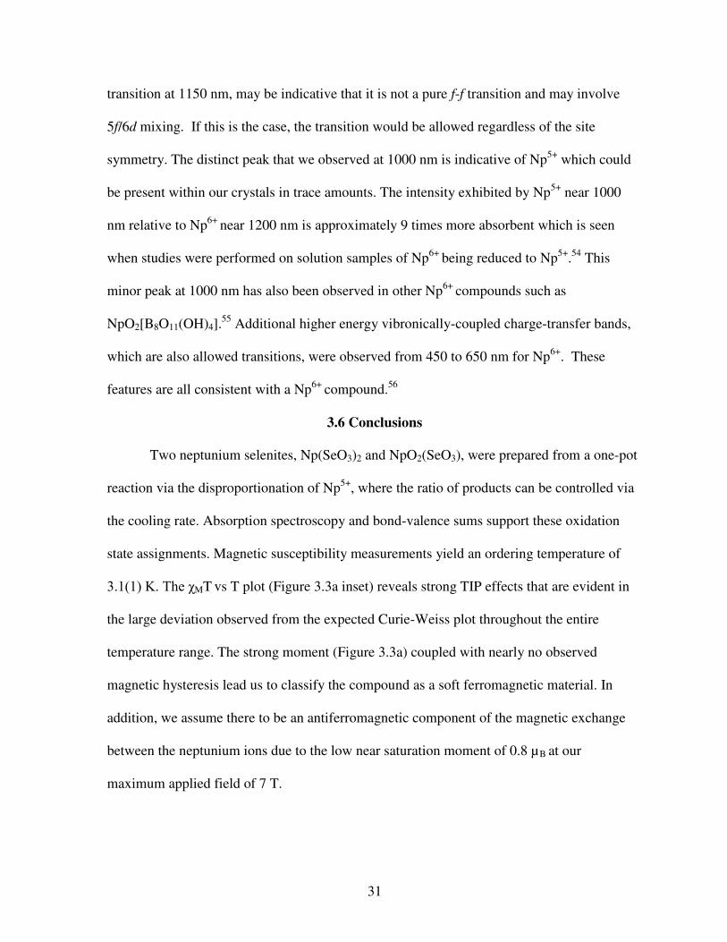
31

transition at 1150 nm, may be indicative that it is not a pure f-f transition and may involve

5f/6d mixing. If this is the case, the transition would be allowed regardless of the site

symmetry. The distinct peak that we observed at 1000 nm is indicative of Np5+ which could

be present within our crystals in trace amounts. The intensity exhibited by Np5+ near 1000

nm relative to Np6+ near 1200 nm is approximately 9 times more absorbent which is seen

when studies were performed on solution samples of Np6+ being reduced to Np5+.54 This

minor peak at 1000 nm has also been observed in other Np6+ compounds such as

NpO2[B8O11(OH)4].55 Additional higher energy vibronically-coupled charge-transfer bands,

which are also allowed transitions, were observed from 450 to 650 nm for Np6+. These

features are all consistent with a Np6+ compound.56

3.6 Conclusions

Two neptunium selenites, Np(SeO3)2 and NpO2(SeO3), were prepared from a one-pot

reaction via the disproportionation of Np5+, where the ratio of products can be controlled via

the cooling rate. Absorption spectroscopy and bond-valence sums support these oxidation

state assignments. Magnetic susceptibility measurements yield an ordering temperature of

3.1(1) K. The χMT vs T plot (Figure 3.3a inset) reveals strong TIP effects that are evident in

the large deviation observed from the expected Curie-Weiss plot throughout the entire

temperature range. The strong moment (Figure 3.3a) coupled with nearly no observed

magnetic hysteresis lead us to classify the compound as a soft ferromagnetic material. In

addition, we assume there to be an antiferromagnetic component of the magnetic exchange

between the neptunium ions due to the low near saturation moment of 0.8 µB at our

maximum applied field of 7 T.

32

Figure 3.4 UV-vis-NIR absorption spectra for Np(SeO3)2 and NpO2(SeO3) at room temperature in the range of 200 nm to 1300 nm along with an image of the crystal that was analyzed.

33

CHAPTER 4

SPIN GLASS AND LONG RANGE FERROMAGNETIC ORDERING EXHIBITED BY NEPTUNIUM IODATES

This chapter covers the synthesis, structural characterization, and magnetic behavior

analysis using direct and alternating current magnetic susceptibility measurements on a novel

neptunium iodate, NpO2(IO3)(H2O)•H2O. In addition, NpO2(IO3) is magnetically analyzed as

a similar comparison. The two neptunium iodates exhibit: cation-cation interactions, formal

oxidation states of +5, ferromagnetic ordering, and spin glass behavior. Having both

ferromagnetic ordering and a spin glass transition is counterintuitive but is shown by a clear

ferromagnetic ordering event at 12 K and frequency dependence of the magnetization with

Mydosh parameters in the range of Φ = 0.03 - 0.05.

4.1 Introduction

Neptunium crystalizes in a wide variety of oxidation states with the Np5+ species

dominating this chemistry because of the stability of this state with respect to

disproportionation.5-7 Neptunium in higher oxidation states tends to adopt highly anisotropic

coordination geometries, primarily due to linear dioxo neptunyl ions, NpO2n+ (n = 1 or 2).

The neptunium ions are further coordinated by four to six additional ligands in a plane

perpendicular to the neptunyl axis yielding tetragonal, pentagonal, and hexagonal

bipyramidal environments surrounding the neptunium centers.8, 9

A wide variety of magnetic behavior is exhibited by neptunium-containing

compounds due in part to its variability of oxidation states and the influences exhibited by

the 5f electrons as discussed in Chapter 1.57-59 Probing the magnetic properties of neptunium

ions with a +5 formal charge ([Rn]5f 2) may seem uninteresting due to its classification as a

34

non-Kramers ion but this is not the case. Experiments have shown long-range ferromagnetic

and antiferromagnetic ordering in Np5+ due to bridging oxo’s that allow for magnetic

superexchange and create unusually short Np···Np distances.60-62 Cation-cation interactions

(CCIs) are evidenced in the neptunium compounds found in this chapter, this term indicates

the alternating direction of the neptunyl bonds within two dimensions. Magnetic ordering

and other phenomenon arise in CCIs composed of neptunium, as the proximity of the metal

centers is increased, these interactions provide a potential superexchange pathway via

oxygen.56, 63 CCIs are in general quite rare but can be found commonly with NpO2+ cations.

The oxygen on the neptunyl bond acts as a ligating ion to the neighboring neptunium.50, 63, 64

Actinide iodates have been studied, in particular those of neptunium, due to their

potential formation within spent nuclear fuel.65, 66 In this chapter, the synthesis, crystal

structures, absorption spectra, and in particular, the magnetic behavior of

NpO2(IO3)(H2O)•H2O is shown to possess both ferromagnetic and spin-glass behavior. In

addition, detailed magnetic susceptibility studies have been performed on NpO2(IO3). These

structure-property correlations extend the available examples of well–characterized 5f

compounds, and assist in our understanding of magnetic coupling occurring in these systems.

4.2 Synthesis and Experimental Descriptions 4.2.1 Synthesis of NpO2(IO3)(H2O)•H2O

NpO2 (0.076 mmol), 1 mL of distilled H2O, and 1 mL of 15.8 M HNO3 were loaded

in a 10-mL PTFE-lined autoclave and kept at 200°C for 24 hours followed by rapid (~1

ºC/min) cooling to room temperature. The reaction of NpO2 with concentrated HNO3 under

mild heating conditions generates a brown solution of mostly Np4+ and Np5+ with some Np6+.

By further heating the brown solution, NO2 gas is released and the concentraded bright pink

35

powder that remains is Np6+ as NpO2(OH)2. 333 L of water was combined with the light

pink NpO2(OH)2 and then loaded into a 10-mL PTFE-lined autoclave with I2O5 (0.241

mmol) and heated for 3 days at 200°C with fast cooling (~1 ºC/min) to room temperature.

With I2O5 added, the solution immediately turns a brilliant green color, hinting to Np5+

formation. The reaction vessel was then allowed to sit at room temperature for one week

before being disturbed. The majority of the solution was removed from the crystals, and

water was added to keep the crystals under solution. The resulting products consisted of

NpO2(IO3)(H2O)•H2O and NpO2(IO3)2 in a 1:1 ratio.

4.2.2 Synthesis of NpO2(IO3)

NpO2(IO3) was synthesized via the combination of NpO2 (0.0357 mmol), I2O5

(0.0491 mmol) and 333 L of distilled H2O. These were heated in a 10-mL PTFE-lined

autoclave for 3 days at 180°C followed by fast cooling (~1 ºC/min) to room temperature.

This yielded a large cluster of polycrystalline NpO2(IO3). These crystals appear to be a

lighter green color than the darker hydrated form. We were able to previously synthesis

NpO2(IO3) using a slightly different procedure.67

4.2.3 Magnetic Susceptibility Measurements

Magnetization measurements were conducted on 3.5 mg of polycrystalline

NpO2(IO3)(H2O)•H2O and 2.3 mg of NpO2(IO3). ZFC and FC measurements were performed

under a constant direct-current (DC) over the temperature range of 1.8 K - 300 K. The

alternate-current (AC) magnetic susceptibilities were measured under various DC bias fields

in the temperature range of 1.8 K - 20 K, with the frequency of AC field varied from 1 to

1000 Hz. Isothermal field dependence of magnetization measurements were performed with

the magnetic field varying between 0 and 5. 5 T at 1.8 K, as well as for hysteresis

36

measurements. Tightly screw-able Teflon sample holders were used to contain our

radioactive samples as described in Chapter 2.

4.3 Crystal Structure Analyses

Single crystals of NpO2(IO3)(H2O)•H2O and NpO2(IO3) were mounted on CryoLoops

with viscous Krytox oil and optically aligned on our X-ray diffractometer at room

temperature. QUEST software was then used to determine the unit cells. The intensities of

reflections of a sphere were collected by a combination of four sets of exposures (frames).

Each set had a different φ angle for the crystal, and each exposure covered a range of 0.5° in

ω. A total of 1464 frames were collected with an exposure time per frame of 10s. Selected

crystallographic information is listed in Table 4.1.

Compound NpO2(IO3)(H2O)•H2O Formula Mass 475.90 Color Light green Habit Prism Space Group P21 a (Å) 5.9070 (8) b (Å) 5.6368 (8) c (Å) 9.6741 (13) β (deg) 97.910 (3) V (Å3) 319.05 (8) Z 2 T (K) 296 λ (Å) 0.71073 Maximum θ (deg.) 26.365 ρcalcd (g/cm3) 4.954 µ (Mo Kα) (cm−1) 21.099 R(F) for Fo

2 > 2σ (Fo2)a 0.0336

Rw(Fo2)b 0.0829

Table 4.1 Selected crystallographic data for the structure NpO2(IO3)H2O•H2O

37

Single crystal X-ray diffraction reveals that NpO2(IO3)(H2O)•H2O crystallizes in the

noncentrosymmetric, monoclinic space group P21. It features a layered structure with cation-

cation interactions between neptunium centers (Figure 4.1a). The layers consist of corner-

sharing NpO7 units with a pentagonal bipyramidal geometry extending along the a-b plane,

as shown in Figure 4.1. One of the oxygen atoms, O1W, on the neptunium units is slightly

longer than the other oxygen atoms on this equatorial axis and is due to the oxygen being part

of a water molecule. Linking the NpO7 units to one another are IO3- anions which are located

in the interstitial space between neptunium layers. H2O molecules can also be found between

layers. Selected bond distances for NpO2(IO3)(H2O)•H2O are given in Table 4.2.

The two axial Np≡O bond distances of the neptunyl unit are 1.827 (2) Å and 1.887

(2) Å; whereas the equatorial Np–O bond distances range from 2.408(2) to 2.471(2) Å. The

IO31− anions adopt the standard trigonal pyramid geometry with approximate C3v symmetry.

I−O bonds, where the oxygen is coordinating the neptunium ions, have a distance of 1.806 Å.

While O(5), localized between the neptunium layers, is at a distance of 1.813 Å. These bond

lengths are typical to I−O bonds.

4.4 Magnetic Studies

The magnetic susceptibilities,, were measured in the ZFC and FC modes.

Measurements performed under an applied field of 400 Oe reveal a clear deviation between

the two modes of measurements for both NpO2(IO3)(H2O)•H2O and NpO2(IO3) as seen in

Figure 4.2, respectively.

The deviations from typical Curie-Weiss behavior, as seen in the 1/χ versus

temperature inset of Figure 4.2, show the presence of temperature independent paramagnetic

effects, TIP.35, 68, 69

38

The TIP effects were discussed in Chapter 2 and are due to the low lying excited

states known to occur in neptunium complexes.

Figure 4.1 (a) View along the c axis of part of the structure of NpO2(IO3)(H2O)•H2O exhibiting the cation-cation interactions of the NpO7 units which are in green with oxygen atoms shown in red. (b) Layers of corner-sharing NpO7 units extending along the a axis. Neptunium-containing polyhedra are shown in green, oxygen atoms that are part of water molecules are in blue while the rest of the oxygen atoms are red. Iodate anions are purple.

39

Select bond of NpO2(IO3)(H2O)•H2O Distance (Å) Np1—O1iii 2.441 (1) Np1—O1W 2.471 (2) Np1—O2 1.827 (2)

Np1—O2 ii 2.420 (2) Np1—O3 2.408 (2) Np1—O4 1.887 (2) Np1—O4i 2.422 (2)

I1—O1 1.804 (1) I1—O3 1.807 (2) I1—O5 1.811 (1)

Fittings of the data (blue line in the insets of Figure 4.2) were performed using the

modified Curie-Weiss equation:

(4.1)

where C, and θ represent the Curie constant, and the Weiss temperature, respectively. A

Curie constant of 1.4(1) emu/mol is obtained for NpO2(IO3)(H2O)•H2O and 1.3(9) emu/mol

for NpO2(IO3), both of which are reduced relative to the expected value for a free Np5+ ion

(roughly 1.6 emu/mol). The reduced moment is due to the crystal-field potential from the two

neptunyl oxygens, which isolates a Jz = ±4 ground doublet that remains the only populated

state at low temperatures. For all other possible crystal-field doublets the calculated Curie

constant would be much lower (0.73 for Jz = ±3, for example).

It is more difficult to model the non-axial terms of the crystal-field potential, coming

from the other (and more distant) surrounding ligands.

Table 4.2 Selected bond distances surrounding the neptunium and iodine nuclei within the structure of NpO2(IO3)(H2O)•H2O

40

The mean-field ordering model for the ferromagnetic phase (dashed blue line in

Figure 4.3) gives far from excellent results, but at least points out that the results above and

below the ordering temperature are consistent.

The ferromagnetic ordering temperatures for NpO2(IO3)(H2O)•H2O and NpO2(IO3)

occur at a Curie temperature of TC = 12.0(0) K and 11.8(7) K, respectively. The complex

with the larger paramagnetic susceptibility also has the higher ordered moment. These

temperatures were estimated as the point of the maximum absolute value of dFC/dT.

A slight amount of remnant magnetization and coercivity can be seen in the plot of

magnetization as a function of applied magnetic field for both neptunium iodates, classifying

them as soft ferromagnetic materials, Figure 4.4.

Clear steps are observed in the hysteresis loops, insets of Figure 4.4a and Figure 4.4b,

which are due to the stabilization of magnetic spin states. It is unclear where these states arise

from and whether they are due to quantum tunneling of the magnetization.

Figure 4.2 The magnetic susceptibility for (a) NpO2(IO3)(H2O)• H2O and (b) NpO2(IO3) measured under an applied magnetic field of 400 Oe using zero field cooled (red) and field cooled (black). The insets show the inverse susceptibility as a function of temperature.

41

Alternating current (AC) measurements were collected within the range of 1.8 K to

20 K and select ranges are shown in Figure 4.5, collected under an applied field of 5 Oe. Out-

of-phase frequency dependent χ” signals were also found via AC susceptibility, exhibiting

maxima within the range of 9.5 to 11.5 K for frequencies comprised between 1 and 1000 Hz

for both NpO2(IO3)(H2O)•(H2O) and NpO2(IO3).

The maximum of χ” arises at a temperature at which the spin relaxation frequency

coincides with the external magnetic field frequency, .

Figure 4.3 The zero field cooled magnetic susceptibilities for NpO2(IO3) and NpO2(IO3)(H2O)•(H2O) measured under a field of 100 Oe. The dashed blue line represents the mean-field ordering model.

42

The thermal relaxation time of magnetization (τ) obeys the Arrhenius lawμ

(4.2)

where τ = 1/2π • and k is the Boltzmann constant. Ueff denotes the effective barrier to

magnetization relaxation. Figure 4.6c and Figure 4.6f display the fitted Arrhenius equations.

Utilizing a linear fitting to the Arrhenius law, an energy barrier of 380 K is yielded for

NpO2(IO3)(H2O)•H2O and 860 K for NpO2(IO3). Although these energy barriers are

relatively high, they represent the purely thermal relaxation barrier and are not the only

pathway to magnetic relaxation. Thus, in terms of field dependent magnetization, the

compounds do not ensure large hysteresis loops.

Figure 4.4 The isothermal field dependence of (a) NpO2(IO3)(H2O)•H2O and (b) NpO2(IO3) measured at 1.8 K. The insets display the magnetic hysteresis near 0 applied magnetic field, highlighting the slight amount of remnant magnetization and coercivity.

43

Interestingly, the peaks in the out-of-phase component, χ”, for the

NpO2(IO3)(H2O)•H2O split into two peaks indicating two distinct magnetic species with

different blocking temperatures as the frequency is increased. These two species differ by

their magnetic relaxation times with increased frequencies favoring the higher temperature

phase. NpO2(IO3), on the other hand, exhibits a large broadening of the out-of-phase signal at

lower frequencies.

A quantitative measure for understanding the magnetic spin dynamics can be

ascertained via the Mydosh parameter:

[ ] (4.3)

Figure 4.5 The real component of the alternating current magnetic susceptibility is plotted for (a) NpO2(IO3)(H2O)•H2O and (d) NpO2(IO3). The imaginary components, χ”, of the AC magnetic susceptibility for (b) NpO2(IO3)(H2O)•H2O and (e) NpO2(IO3). The various colors and shapes represent the different frequencies of the driving field as detailed in the legend. Finally, the Arrhenius fittings to the plots of the imaginary component are shown in (c) NpO2(IO3)(H2O)•H2O and (f) NpO2(IO3).

44

TSG represents the temperature at which the maximum in χ”(T) occurs, ∆TSG is the difference

in TSG between an initial frequency, ω, and final frequency, ωf, and ∆(log ω) is the difference

between the log of the initial and final measuring frequencies.70-73 The value of Φ obtained

for NpO2(IO3)(H2O)•H2O is approximately Φ = 0.03 for the lower temperature peak and Φ =

0.05 for the higher temperature. NpO2(IO3) has a Mydosh parameter of Φ = 0.05. The

Mydosh parameters vary slightly from the expected range of 0.004–0.018 for conventional

spin glass systems. Our Φ values deem the materials slightly less dynamic than conventional

spin glasses but significantly less than 0.1 expected for superparamagnetic materials.73

4.5 Conclusions

This chapter highlighted two synthesized neptunium iodate complexes,

NpO2(IO3)(H2O)•H2O and NpO2(IO3) of which the hydrated sample is novel. These

compounds were synthesized and then structurally characterized using scXRD and

magnetically characterized using alternating current and direct current magnetic

susceptibility. Both materials exhibit ferromagnetic ordering near 12 K with negligible

hysteresis, characterizing them as soft ferromagnetic materials. Water molecules and the

distance between neptunium layers are what vary the two compounds structurally while

ferromagnetic ordering and frequency dependent magnetic susceptibility occur in both.

Ferromagnetic exchange and thus ordering can be attributed to taking place within the layer

due to the independence of distance between layers. The alternating current magnetic

susceptibility differs, with the non-hydrated neptunium iodate broadening at lower

frequencies while the hydrated sample displays two distinct magnetic phases, with a

45

preference for the higher blocking temperature as the frequency is increased. The calculated

Mydosh parameters confirm the both neptunium iodates as spin glass materials.

46

CHAPTER 5

STRUCTURE-PROPERTY RELATIONSHIPS IN LANTHANIDE COPPER SULFATE HETEROBIMETALLIC COMPOUNDS

This chapter encapsulates a large family of lanthanide copper heterobimetallic

compounds that display interesting magnetic properties. Unfortunately, several of the

compounds were isolated in quantities only suitable for structural analysis and thus were not

magnetically probed. Magnetic properties ranging from ferromagnetic to antiferromagnetic

ordering as well as deviations from typical Curie-Weiss behavior are shown. This chapter

also correlates the lanthanide contraction’s effect on the crystal structure and how this alters

the observed magnetic properties.

5.1 Introduction The concept of rational design of 3d/4f heterobimetallic materials has attracted much

attention because of the potential of these materials in various applications, for instance:

single molecule magnets (SMMs),74-77 ion exchange,78 and optical sensing,79 as mentioned in

Chapter 1. Due to their high coordination numbers and varied magnetic properties, the

lanthanide series is likely to provide new materials that possess advantageous properties and

desired features. In addition, the structural chemistry of lanthanides is rich owing to their

different coordination geometries and the lanthanide contraction. The highly systematic

reduction in ionic radii that occurs across the 4f series allows one to observe phase changes

induced by very small changes in ion sizes. Examples of these include Ln(OH)SO4 (Ln = Pr-

Yb, except Pm), [Ln(INO)(H2O)(SO4)]n (Ln = La-Yb, except Pm), Ln2Cu(TeO3)2(SO4)2 (Ln

= Y, Nd, Sm, Eu, Gd, Tb, Dy, Ho, Er, Tm, Yb, and Lu), etc. This large family of lanthanide

tellurite sulfates is particularly interesting because it shows a rare case of dimensional and

47

coordination number reductions between five different phases due to the lanthanide

contraction. Different magnetic properties arise between those different phases even with the

same lanthanide ion. This chapter highlights the differences between two compounds, both

contatining gadolinium and copper, that display different amounts of magnetic coupling due

to structural correlations.

While lanthanide intermetallic compounds have played keys roles in the development

of magneto-structural correlations, oxoanion systems are also extremely well developed.80-88

The solid state chemistry of sulfate is intricate owning to the following reasons. Sulfate can

coordinate with metal ions in versatile manners, including terminal monodentate, terminal

bidentate, bridging bidentate, and bridging tridentate, contributing to the complexity and

intricacy of structures.89 A diversity of topologies, including one-dimensional (1D) chain,

two-dimensional (2D) layered structures, and three-dimensional (3D) frameworks have been

achieved in lanthanide sulfate complexes.90-92 Sulfate has been proved to be an excellent

bridging ligand in construction of transition-metal hydroxysulfates.93-95 The exceptional

abilities of sulfate ion bridging two or more metallic centers make sulfate as an ideal ligand

for the synthesis of 3d/4f heterobimetallic compounds. Indeed, a series of 3d−4f

hydroxysulfates Ln2Cu(SO4)2(OH)4 (Ln = Sm, Eu, Tb, Dy) have been successfully obtained

hydrothermally.

Applying the aforementioned sulfate to the study of 3d/4f heterobimetallic materials

is a promising route of creating new solids with interesting physico-chemical properties. In

an attempt to prepare lanthanide-containing materials that allow for comparisons in bonding

and physical properties, a large family of lanthanide copper sulfates, with four different

topologies, Ln2Cu(SO4)2(OH)4 (Ln = Sm, Eu, Gd, Dy, and Ho) (LnCuSO4-1),

48

Ln4Cu(SO4)2(OH)10 (Ln = Tm, Yb, and Lu) (LnCuSO4-2), LnCu(SO4)(OH)3 (Ln = Nd, Sm,

Eu, and Gd) (LnCuSO4-3), and LnCu(SO4)(OH)3 (Ln = Dy, Ho, Yb, Er, Tm, Yb, and Lu)

(LnCuSO4-4) were discovered. The remainder of this chapter describes the preparation,

structure elucidation, and magnetic properties of this family of complexes.

5.2 Synthesis and Experimental Descriptions

Nd2O3 (99.9 %, Alfa-Aesar), Sm2O3 (99.9 %, Alfa-Aesar), Eu2O3 (99.9 %, Alfa-

Aesar), Gd2O3 (99.9 %, Alfa-Aesar), Dy2O3 (99.9 %, Alfa-Aesar), Ho2O3 (99.9 %, Alfa-

Aesar), Er2O3 (99.9 %, Alfa-Aesar), Tm2O3 (99.9 %, Alfa-Aesar), Yb2O3 (99.9 %, Alfa-

Aesar), Lu2O3 (99.9 %, Alfa-Aesar), CuO (99.99 %, Sigma-Aldrich), and concentrated

H2SO4 (98%, Alfa-Aesar) were all used as received. Reactions were run in PTFE-lined Parr

4749 autoclaves with 23 mL internal volume autoclaves. Distilled and Millipore filtered

water was used in all reactions.

The four various structure types were synthesized using these methods:

Ln2Cu(SO4)2(OH)4 (Ln = Sm, Eu, Gd, Dy, and Ho) (LnCuSO4-1). Ln2O3 (1 mmol), CuO (1

mmol), and 1 M H2SO4 (2 mmol) were loaded into a 23 mL PTFE-lined autoclave liner.

Ln4Cu(SO4)2(OH)10 (Ln = Tm, Yb, and Lu) (LnCuSO4-2). Ln2O3 (2 mmol), CuO (1 mmol,

0.0795 g), and 1 M H2SO4 (2 mmol) were loaded. LnCu(SO4)(OH)3 (Ln = Nd, Sm, Eu, and

Gd) (LnCuSO4-3). Ln2O3 (0.5 mmol), CuO (1 mmol), 1 M H2SO4 (1 mmol), and 1 mL water

were loaded. LnCu(SO4)(OH)3 (Ln = Dy, Ho, Yb, Er, Tm, Yb, and Lu) (LnCuSO4-4). Ln2O3

(0.5 mmol), CuO (1 mmol), 1 M H2SO4 (1 mmol), and water were loaded into the liner. The

autoclave liners were sealed and heated to 230 °C for 3 days followed by slow cooling to

room temperature at a rate of 5 °C/hr. The products were washed with DI water to remove

soluble solids, followed by rinsing with ethanol.

49

The crystals of LnCuSO4-1, LnCuSO4-2, LnCuSO4-3, and LnCuSO4-4 were

successfully synthesized by reacting CuO and H2SO4 (1M) with the corresponding lanthanide

oxide using hydrothermal conditions (Figure 5.1). LnCuSO4-1 is a minor product and

consisted of dark blue tablet crystals, coexisting with LnCuSO4-3. LnCuSO4-2 is the main

product with yields ranging from 40 % to 50 %, consisting of purple tablet crystals.

LnCuSO4-3 and LnCuSO4-4 form as light blue prismatic crystals with yields ranging from

60% to 70%, coexisting in some cases with unreacted CuO. The formation of LnCuSO4-2,

LnCuSO4-3, and LnCuSO4-4 are found to be stoichiometrically driven. All of the compounds

were obtained with the highest yields when the reactants have the same molar ratio of

Ln/Cu/S as the products. The Sm, Eu, and Dy analogues of LnCuSO4-1 have been reported

recently using a different synthesis method.96

5.3 Structural Descriptions

Single crystal X-ray diffraction reveals that LnCuSO4-1 and LnCuSO4-2 crystalize in

the monoclinic space groups P21/c and P21/n, respectively. The building blocks of these two

3D frameworks are lanthanide polyhedra, copper ions, and sulfate tetrahedra. The SO42-

tetrahedra chelate the lanthanide centers, but they do not fill all of the space in the

framework, as a consequence of this architecture, a system of channels extending down the a

axis are observed in LnCuSO4-1 (Figure 5.2a) and LnCuSO4-2 (Figure 5.2b). The polyhedral

connectivity in the channel architectures of LnCuSO4-1 and LnCuSO4-2 involves both edge-

sharing and face-sharing of lanthanide centers. A ball-stick view of the cross-section of the

channels is shown in Figure 5.3a for LnCuSO4-1 and Figure 5.3b for LnCuSO4-2. For

LnCuSO4-1, the channels are composed of six-membered Ln rings with Ln atoms connected

to each other via oxygen bridges.

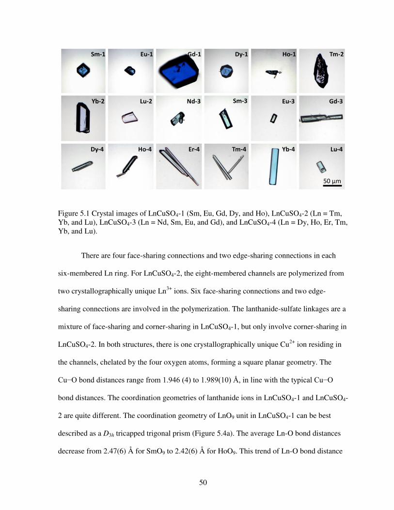
50

There are four face-sharing connections and two edge-sharing connections in each

six-membered Ln ring. For LnCuSO4-2, the eight-membered channels are polymerized from

two crystallographically unique Ln3+ ions. Six face-sharing connections and two edge-

sharing connections are involved in the polymerization. The lanthanide-sulfate linkages are a

mixture of face-sharing and corner-sharing in LnCuSO4-1, but only involve corner-sharing in

LnCuSO4-2. In both structures, there is one crystallographically unique Cu2+ ion residing in

the channels, chelated by the four oxygen atoms, forming a square planar geometry. The

Cu−O bond distances range from 1.946 (4) to 1.989(10) Å, in line with the typical Cu−O

bond distances. The coordination geometries of lanthanide ions in LnCuSO4-1 and LnCuSO4-

2 are quite different. The coordination geometry of LnO9 unit in LnCuSO4-1 can be best

described as a D3h tricapped trigonal prism (Figure 5.4a). The average Ln-O bond distances

decrease from 2.47(6) Å for SmO9 to 2.42(6) Å for HoO9. This trend of Ln-O bond distance

Figure 5.1 Crystal images of LnCuSO4-1 (Sm, Eu, Gd, Dy, and Ho), LnCuSO4-2 (Ln = Tm, Yb, and Lu), LnCuSO4-3 (Ln = Nd, Sm, Eu, and Gd), and LnCuSO4-4 (Ln = Dy, Ho, Er, Tm, Yb, and Lu).

51

is consistent with the increasing localization and decreased shielding of the 4f orbitals given

the consequent ionic contraction. Both crystallographically unique Ln3+ centers in LnCuSO4-

2 are coordinated by eight oxygen atoms, forming square antiprism with approximate D4d

symmetry. A similar ionic radius decreasing trend was observed in this structure type due to

the lanthanide contraction.

Figure 5.2 View of the structures of (a) LnCuSO4-1 (Sm, Eu, Gd, Dy, and Ho), (b) LnCuSO4-2 (Ln = Tm, Yb, and Lu), (c) LnCuSO4-3 (Ln = Nd, Sm, Eu, and Gd), and (d) LnCuSO4-4 (Ln = Dy, Ho, Er, Tm, Yb, and Lu). Lanthanide polyhedra are shown in dark blue, pink, cyan, and purple in LnCuSO4-1, LnCuSO4-2, LnCuSO4-3, and LnCuSO4-4, respectively. Copper ions are shown in dark blue with sulfate tetrahedra in gray.

52

Figure 5.3 Structures of (a) LnCuSO4-1 (Sm, Eu, Gd, Dy, and Ho), (b) LnCuSO4-2 (Ln = Tm, Yb, and Lu), (c) LnCuSO4-3 (Ln = Nd, Sm, Eu, and Gd), and (d) LnCuSO4-4 (Ln = Dy, Ho, Er, Tm, Yb, and Lu). These structures emphasize the connectivities of Ln polyhedra bridged by oxygen atoms. Lanthanide ions are shown in dark blue, pink, cyan, and purple in LnCuSO4-1, LnCuSO4-2, LnCuSO4-3, and LnCuSO4-4, respectively. Oxygen atoms are in red.

53

Both LnCuSO4-3 and LnCuSO4-4 crystalize in the space group, Pnma. Although they

have the identical molecular formula and the same space group, their crystallographic

parameters and topologies are different. The analogous yttrium structures for LnCuSO4-3 and

LnCuSO4-4 have been previously synthesized with a general formula of YM(OH)3(SO4) (M

= Ni, Cu), but the lanthanide structures in this chapter are novel.97, 98 The structures of

LnCuSO4-3 and LnCuSO4-4 are constructed from Ln polyhedra, distorted CuO6 octahedra,

and SO42- tetrahedra, to fom 3D frameworks (Figure 5.2c and Figure 5.2d). For LnCuSO4-3,

the Ln polyhedra face-share creating one dimensional (1D) chains extending along the a-axis

(Figure 5.3c). For LnCuSO4-4, zigzagging chains are formed along the b axis and each Ln

polyhedra edge-share with the nearest neighbors (Figure 5.3d). The Ln polyhedra chains are

corner-shared by SO42- tetrahedra and are further chelated by Cu2+ ions, forming 3D

frameworks. Compared with the square planar geometries of Cu2+ in LnCuSO4-1 and

LnCuSO4-2, the Cu2+ coordination geometries in LnCuSO4-3 and LnCuSO4-4 are

significantly different and can be described as Jahn−Teller distorted octahedra. The axial

Cu−O bonds are between 2.320(2) Å and 2.471(3) Å with the equatorial Cu−O bonds

ranging from 1.947(2) Å to 1.983(3) Å. Coordination of Ln in LnCuSO4-3 and LnCuSO4-4

varies as well. The geometry of LnO9 in LnCuSO4-3 is described as a D3h tricapped trigonal

prism (Figure 5.4c), with average Ln-O bond distances decrease from 2.53(10) Å for NdO8 to

2.49(11) Å for GdO8. The geometry of LnO8 unit in LnCuSO4-4 can be described as a D4d

square antiprism (Figure 5.4d). The average Ln-O bond distances decrease from 2.38(2) Å

for DyO8 to 2.33(3) Å for LuO8.

54

5.4 Periodic Trends

This chapter consists of a large family of 3D lanthanide copper compounds and

demonstrates a clear effect of lanthanide contraction resulting in two structural topologies in

two different pathways (LnCuSO4-1→LnCuSO4-2 and LnCuSO4-3→LnCuSO4-4). More

specifically, the effect of the lanthanide contraction is reflected in: the decreasing volume of

the unit cells within the same structure type, the decreasing Ln−O bonding distance, and the

Figure 5.4 Representation of the coordination geometries of lanthanide ions in (a) LnCuSO4-1 (Sm, Eu, Gd, Dy, and Ho), (b) LnCuSO4-2 (Ln = Tm, Yb, and Lu), (c) LnCuSO4-3 (Ln = Ln = Nd, Sm, Eu, and Gd), and (d) LnCuSO4-4 (Ln = Dy, Ho, Er, Tm, Yb, and Lu).

55

decreasing coordination number of the lanthanides. The coordination numbers of lanthanides

decrease from nine (LnCuSO4-1 and LnCuSO4-3) to eight (LnCuSO4-2 and LnCuSO4-4)

from the early lanthanides to late lanthanides. Raymond’s study suggests that the inverse of

lanthanide ionic radii as a function of valence f electron number gives a linear fit for a variety

of lanthanide complexes.99 The ionic radii of Ln3+ in those lanthanide copper sulfates were

obtained by subtracting the ionic radius of O2- ions from the Ln−O distances. Nearly linear

trends relating Ln ionic radius versus the numbers of f electrons were observed for LnCuSO4-

1, LnCuSO4-2, LnCuSO4-3, and LnCuSO4-4, and are shown in Figure 5.5. For lutetium to

adopt the LnCuSO4-1 and LnCuSO4-3 structure types, an ionic radius of 1.12 Å and 1.16 Å

would be required, based on the equations y = 0.0082 x + 0.782 and y = 0.0067 x + 0.7686,

respectively. The effective ionic radius for nine−coordinate Lu3+ is typically 1.032 Å.16 The

crystal lattices of LnCuSO4-1 and LnCuSO4-3 are experiencing increasing strain with

decreasing ionic radius, resulting in the phase transitions for the late lanthanides.

5.5 Analysis of Magnetic Susceptibility and Magnetization

Owing to the magnetic interactions that could arise as a result of the presence of 3d/4f

unpaired electrons and multiple bonding geometries between them, direct current magnetic

susceptibility studies of GdCuSO4-1, GdCuSO4-3, YbCuSO4-2, YbCuSO4-4, and HoCuSO4-

4 were investigated. The other samples are not included due to their relatively low yields or

the presence of impurities. The examined compounds are directly compared as they possess

the same spins with different connectivities or different magnetic ions in an isostructural

arrangement.

56

Figure 5.5 Plots of the inverse of the ionic radii versus the number of the f electrons for (a) LnCuSO4-1 (Sm, Eu, Gd, Dy, and Ho) and LnCuSO4-2 (Ln = Tm, Yb, and Lu); (b) LnCuSO4-3 (Ln = Ln = Nd, Sm, Eu, and Gd) and LnCuSO4-4 (Ln = Dy, Ho, Er, Tm, Yb, and Lu).

57

As shown in Figure 5.6a, GdCuSO4-1 exhibits typical paramagnetic behavior and no

evidence of long-range ordering was observed in the temperature range 1.8–300 K. The data

were fitted over the entire temperature range using the Curie–Weiss law, Figure 5.6b. The

effective moment was evaluated from the Curie constant by:

(5.1)

where N, µB, and kB are Avogadro’s number, Bohr magneton, and Boltzmann constant,

respectively. The μeff for GdCuSO4-1 determined via the Curie-Weiss fitting is 11.4(1) μB

which corresponds well to the value of 11.49 μB expected for two Gd3+ ions (J = 7/2, g = 2.0)

and one Cu2+ ion (S = 1/2, g = 2.0). The slope of 1/ remains essentially constant throughout

the measured temperature range with a small negative Weiss temperature, θ = –1.1(5) K,

indicating a lack of strong nearest neighbor interactions. Gd3+ has the largest spin moment (S

= 7/2) of the lanthanides with no net orbital momentum (L = 0).100 There is no anisotropy of

the charge and correspondingly no crystal field splitting. Consequently, the field-dependent

magnetization of GdCuSO-1 at 1.8 K is in good agreement with the sum of Brillouin

functions for two paramagnetic Gd3+ ions and one Cu2+ ion (Figure 5.6c). Similar behavior

has been observed in Gd2Cu(TeO3)2(SO4)2. GdCuSO4-3 differs from GdCuSO4-1 in terms of

structural and magnetic properties. GdCuSO4-1 contains two crystallographically unique

Gd3+ ions while GdCuSO4-3 has one, with shorter bond distances connecting the magnetic

ions. The low temperature magnetic susceptibility of GdCuSO4-3 indicates a ferromagnetic

phase transition at 8 K, which is seen by the bifurcation arising between the zero field-cooled

and field-cooled susceptibility measurements (Figure 5.7a).

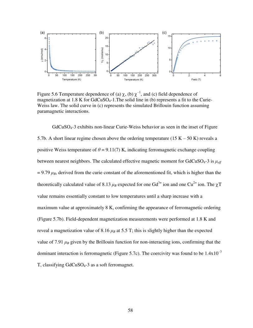
58

GdCuSO4-3 exhibits non-linear Curie-Weiss behavior as seen in the inset of Figure

5.7b. A short linear regime chosen above the ordering temperature (15 K – 50 K) reveals a

positive Weiss temperature of θ = 9.11(7) K, indicating ferromagnetic exchange coupling

between nearest neighbors. The calculated effective magnetic moment for GdCuSO4-3 is μeff

= 9.79 μB, derived from the curie constant of the aforementioned fit, which is higher than the

theoretically calculated value of 8.13 μB expected for one Gd3+ ion and one Cu2+ ion. The T

value remains essentially constant to low temperatures until a sharp increase with a

maximum value at approximately 8 K, confirming the appearance of ferromagnetic ordering

(Figure 5.7b). Field-dependent magnetization measurements were performed at 1.8 K and

reveal a magnetization value of 8.16 μB at 5.5 T; this is slightly higher than the expected

value of 7.91 μB given by the Brillouin function for non-interacting ions, confirming that the

dominant interaction is ferromagnetic (Figure 5.7c). The coercivity was found to be 1.4x10–3

T, classifying GdCuSO4-3 as a soft ferromagnet.

Figure 5.6 Temperature dependence of (a) , (b) –1, and (c) field dependence of magnetization at 1.8 K for GdCuSO4-1.The solid line in (b) represents a fit to the Curie-Weiss law. The solid curve in (c) represents the simulated Brillouin function assuming paramagnetic interactions.

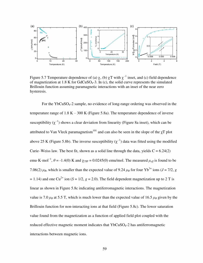
59

For the YbCuSO4-2 sample, no evidence of long-range ordering was observed in the

temperature range of 1.8 K – 300 K (Figure 5.8a). The temperature dependence of inverse

susceptibility (–1) shows a clear deviation from linearity (Figure 8a inset), which can be

attributed to Van Vleck paramagnetism101 and can also be seen in the slope of the χT plot

above 25 K (Figure 5.8b). The inverse susceptibility (–1) data was fitted using the modified

Curie–Weiss law. The best fit, shown as a solid line through the data, yields C = 6.24(2)

emu·K·mol−1, θ = -1.4(0) K and TIP = 0.0245(0) emu/mol. The measured μeff is found to be

7.06(2) μB, which is smaller than the expected value of 9.24 μB for four Yb3+ ions (J = 7/2, g

= 1.14) and one Cu2+ ion (S = 1/2, g = 2.0). The field dependent magnetization up to 2 T is

linear as shown in Figure 5.8c indicating antiferromagnetic interactions. The magnetization

value is 7.0 μB at 5.5 T, which is much lower than the expected value of 16.5 μB given by the

Brillouin function for non-interacting ions at that field (Figure 5.8c). The lower saturation

value found from the magnetization as a function of applied field plot coupled with the

reduced effective magnetic moment indicates that YbCuSO4-2 has antiferromagnetic

interactions between magnetic ions.

Figure 5.7 Temperature dependence of (a) , (b) T with –1 inset, and (c) field dependence of magnetization at 1.8 K for GdCuSO4-3. In (c), the solid curve represents the simulated Brillouin function assuming paramagnetic interactions with an inset of the near zero hysteresis.

60

Unlike YbCuSO4-2, YbCuSO4-4 exhibits a clear antiferromagnetic transition. The

transition occurs at 6.3 K, (Figure 5.9a), as clearly seen by the field cooled and zero field

cooled plots of magnetic susceptibility as a function of temperature. Above 10 K, the –1

obeys the modified Curie–Weiss law and a fitting from 10 to 250 K yields values of C =

1.35(2) emu·K·mol−1, θ = -2.1(5) K and TIP = 0.00453(8) emu/mol. The measured μeff =

3.29(4) μB is lower than the calculated value of 4.86 μB for one Yb3+ ion (J = 7/2, g = 1.14)

and one Cu2+ ion (S = 1/2, g = 2.0). Field-dependent magnetization measurements were

performed at 1.8 K, providing further evidence of antiferromagnetic interactions with a linear

fit up to 0.6 T (Figure 5.9c).

Although in an analogous structure type to YbCuSO4-4, the holmium analogue

displays ferromagnetic ordering instead of antiferromagnetic ordering. The effective

magnetic moment at 300 K for HoCuSO4-4 is μeff = 13.15 μB, which is greater than the

expected value of 10.74 μB for one Ho3+ ion (J = 8, g = 1.25) and one Cu2+ ion (S = ½, g =

2.0), suggesting ferromagnetic interactions.

Figure 5.8 Temperature dependence of (a) with an inset of –1, (b) T, and (c) field dependence of magnetization at 1.8 K for YbCuSO4-2. In (c), the solid curve represents the simulated Brillouin function assuming paramagnetic interactions while the solid line represents a linear fit in that regime.

61

Figure 5.10a displays the bifurcation of the zero field cooled and field cooled data for

HoCuSO4-4 yielding a ferromagnetic ordering temperature of 3.6 K. The steep slope of the

magnetization value at high fields suggests the magnetization will saturate above the

expected value of the Brillouin function (Figure 5.10c). A lack of appreciable coercivity

indicates soft ferromagnetic behavior.

5.6 Electron Paramagnetic Resonance

Gadolinium and copper are both expected to adhere linearly with Curie-Weiss fittings

as observed for GdCuSO4-1, Figure 5.6. However, GdCuSO4-3 exhibits a strong deviation

Figure 5.9 Temperature dependence of (a) , (b) –1 with a solid line fit to the Curie-Weiss law, and (c) field dependence of magnetization at 1.8 K for YbCuSO4-4. In (c), the solid curve represents the simulated Brillouin function assuming paramagnetic interactions.

Figure 5.10 Temperature dependence of (a) , (b) T, (c) field dependent magnetization for HoCuSO4-4 with the solid curve represents the simulated Brillouin function assuming paramagnetic interactions while the solid line represents a linear fit in that regime.

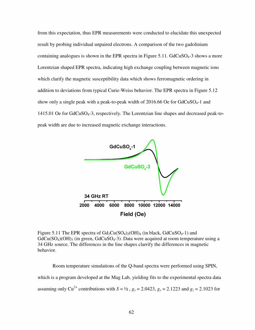
62

from this expectation, thus EPR measurements were conducted to elucidate this unexpected

result by probing individual unpaired electrons. A comparison of the two gadolinium

containing analogues is shown in the EPR spectra in Figure 5.11. GdCuSO4-3 shows a more

Lorentzian shaped EPR spectra, indicating high exchange coupling between magnetic ions

which clarify the magnetic susceptibility data which shows ferromagnetic ordering in

addition to deviations from typical Curie-Weiss behavior. The EPR spectra in Figure 5.12

show only a single peak with a peak-to-peak width of 2016.66 Oe for GdCuSO4-1 and

1415.01 Oe for GdCuSO4-3, respectively. The Lorentzian line shapes and decreased peak-to-

peak width are due to increased magnetic exchange interactions.

Room temperature simulations of the Q-band spectra were performed using SPIN,

which is a program developed at the Mag Lab, yielding fits to the experimental spectra data

assuming only Cu2+ contributions with S = ½ , gx = 2.0423, gy = 2.1223 and gz = 2.1023 for

Figure 5.11 The EPR spectra of Gd2Cu(SO4)2(OH)4 (in black, GdCuSO4-1) and GdCu(SO4)(OH)3 (in green, GdCuSO4-3). Data were acquired at room temperature using a 34 GHz source. The differences in the line shapes clarrify the differences in magnetic behavior.

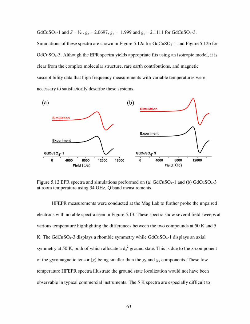
63

GdCuSO4-1 and S = ½ , gx = 2.0697, gy = 1.999 and gz = 2.1111 for GdCuSO4-3.

Simulations of these spectra are shown in Figure 5.12a for GdCuSO4-1 and Figure 5.12b for

GdCuSO4-3. Although the EPR spectra yields appropriate fits using an isotropic model, it is

clear from the complex molecular structure, rare earth contributions, and magnetic

susceptibility data that high frequency measurements with variable temperatures were

necessary to satisfactorily describe these systems.

HFEPR measurements were conducted at the Mag Lab to further probe the unpaired

electrons with notable spectra seen in Figure 5.13. These spectra show several field sweeps at

various temperature highlighting the differences between the two compounds at 50 K and 5

K. The GdCuSO4-3 displays a rhombic symmetry while GdCuSO4-1 displays an axial

symmetry at 50 K, both of which allocate a dz2 ground state. This is due to the z-component

of the gyromagnetic tensor (g) being smaller than the gx and gy components. These low

temperature HFEPR spectra illustrate the ground state localization would not have been

observable in typical commercial instruments. The 5 K spectra are especially difficult to

Figure 5.12 EPR spectra and simulations preformed on (a) GdCuSO4-1 and (b) GdCuSO4-3 at room temperature using 34 GHz, Q band measurements.

64

interpret due to small crystallites, magnetic exchange coupling between gadolinium and

copper ions, and intermolecular interactions.

Variable temperature (5 K to 290 K) measurements at 240GHz show the linewidth

varying with temperature for the two compounds with the maximum occurring near 75 K,

which may be due to a magnetic phase transition, shown in Figure 5.14; it is below this

temperature where the isotropic g tensor splits into two axial components.

5.7 Conclusions

Magnetic measurements reveal behavior ranging from antiferromagnetic ordering to

ferromagnetic ordering for these heterobimetallic systems, namely the ytterbium and

holmium structural analogues of LnCu(SO4)(OH)3, respectively. The lack of remnant

magnetization and coercivity further classifies this holmium analogue as a soft ferromagnet.

Figure 5.13 High frequency high field EPR spectra of (a) GdCuSO4-1 measured at 50 K and 5 K and (b) GdCuSO4-3 measured at 50 K, 15 K, and 5 K.

65

Surprisingly the gadolinium analogue of LnCu(SO4)(OH)3 displays large deviations

from typical Curie-Weiss behavior, which are characteristic to both copper and gadolinium

ions; electron paramagnetic resonance coupled with structural correlations reveal the

deviation to be due to strong magnetic coupling which results in ferromagnetic ordering at 8

K. Further analysis of HFEPR data is still underway including measurements performed at

120 GHz and 336 GHz. Further investigations near 75 K are necessary to explain splitting of

HFEPR data for GdCuSO4-3.

Figure 5.14 Peak to peak linewidths of GdCuSO4-3 as a function of temperature. The maximum peak to peak linewidth occurs near 75 K due to the splitting of the isotropic g tensor.

66

CHAPTER 6

MAGNETIC PROPERTIES OF VARIOUS OTHER SYSTEMS

In addition to the previously discussed compounds, there are also the compounds

found in this chapter, that have interesting magnetic properties such as spin frustration,

magnetic ordering, and a large family of heterobimetallic compounds with varying magnetic

behaviors that are comparable to the compounds in Chapter 5. These works have been

published.102-104 Reprinted in part with permission from Babo, J.-M.; K. Diefenbach; T.E.

Albrecht-Schmitt, Inorg. Chem., 2014, 53 (7), 3540-3545. Copyright 2014 American

Chemical Society. Reprinted in part with permission from Lin, J.; P. Chai; K. Diefenbach; M.

Shatruk; T.E. Albrecht-Schmitt, Chem. Mater., 2014, 26 (6), 2187-2194. Copyright 2014

American Chemical Society. Reprinted in part with permission from Lin, J.; K. Diefenbach;

M.A. Silver; N.S. Dalal; T.E. Albrecht-Schmitt, Cryst. Growth Des., 2015, 15 (9), 4606-

4615. Copyright 2015 American Chemical Society.

6.1 Introduction

A U4+/Sb3+ thiophosphate, Cs6U3Sb2P8S32, containing a novel anion, [Sb(PS4)3]6– ,

was discovered and is shown to have antiferromagnetic ordering at 53 K. In general,

chalcophosphates are able to bind a vast array of main group, transition metal, and f block

cations in both low and high oxidation states.105, 106 Among the richest group of these

compounds, are those containing uranium. Their complexity can be ascribed to several

factors. First, the uranium brings structural intricacy to these systems in that the coordination

chemistry of uranium is extremely flexible and coordination numbers of eight and nine are

typical. Second, the formal oxidation states of uranium vary between +4 and +6. Third, the

uranium cations stabilize a wide variety of thiophosphate anions which leads to an immense

67

structural complexity and new main group chemistry. Examples of this include Rb4U4P4Se26,

which contains uranium in the atypical +5 oxidation state, and A11U7(PS4)13 (A = K, Rb),

which despite containing only isolated [PS4]3–anions forms a fascinating architecture

constructed from interlocked helices.106, 107 Antimony was used to create an even more

complex thiophosphate, which under these synthetic conditions will be Sb3+ and will

therefore possess a lone-pair of electrons that is likely to be stereochemically active, leading

to rich structural chemistry.

The introduction of various spin carriers within the same structure type can lead to a

vast array of magnetic interactions in lanthanide-transition metal heterobimetallic compounds

as previously shown in Chapter 5.108 The diversity of coordination environments exhibited by

lanthanides enables different arrangement between the metal ions, resulting in a variety of

magnetic exchange pathways.109 By incorporating tellurite, a large family of compounds was

formed with various magnetic properties. Tellurite was chosen due to several physical and

chemical reasons: first, tellurite possess a stereochemically active lone pair of electrons and

Te4+ can form TeO32−, TeO4

4−, and TeO56− oxo-anions with asymmetrical geometries.38 Due

to the second-order Jahn–Teller (SOJT ) distortion, tellurite can align in the solid state to

yield noncentrosymmetric structures. Several interesting physical properties, such as

ferroelectricity, pyroelectricity, piezoelectricity, and second-order nonlinear optical behavior

have been observed.110 Second, concomitant with the focus of tellurite’s polarity has been the

combination of other oxo-anions with tellurite to enhance its properties.111 Mixing SOJT

distorted d0 (Mo6+, V5+, Ti4+) oxoanions with tellurites can lead to the formation of structures

with permanent polarization when the asymmetric building units are properly aligned,

resulting in strong second harmonic generation properties.

68

As a byproduct of our reactions containing heterobimetallic compounds with tellurite,

Cu3(TeO4)(SO4)·H2O was formed. In several of the reactions this compound was a side

product which we carefully isolated and found to also be magnetically interesting, displaying

long range magnetic ordering and two structurally and magnetically distinct copper ions.

6.2 Cs6U3Sb2P8S32: A Spin Frustrated System

The formation of Cs6U3Sb2P8S32 came about by a mixture of Cs2S3/U/P2S5/S in a

1:1:2:1 stoichiometric ratio in an evacuated silica glass tube. This sealed ampule was then

slowly heated to 500 °C over a 24 hour period and held there for 5 days. The reaction was

then slow at the rate of 5 °C/h to room temperature. Dark red irregular-shaped crystals of the

title compounds formed. The crystal structure can be seen in Figure 6.1.

Cs6U3Sb2P8S32 contains [U3(PS4)2[Sb(PS4)3]2]6– layers intercalated by Cs+ cations. The layers

are composed of trimeric uranium units connected to each other by the [Sb(PS4)3]6– anion.

Each uranium cation is surrounded by eight sulfide anions in a distorted square antiprism that

shares two edges with two other crystallographically equivalent units to form a trimeric

[U3S18]24– cluster as shown in Figure 6.1.

Based on Russel-Saunders coupling, U4+ has a 3H4 ground term and 5f 2 configuration

classifies the ion as a non-Kramers ion with. Strong magnetic anisotropy is well known to

occur in U4+ containing compounds.112, 113 The temperature dependencies of the molar

magnetic susceptibility, χM, were measured yielding a sharp cusp noted at approximately 53

K which may occur due to spin frustration occurring within the uranium trimers or

paramagnetic oxygen leaking into the system which would exhibit a signal at this

temperature.114, 115 To confirm the signal is not due to an oxygen impurity, FC and ZFC

measurements at field strengths of 0.1 T, 0.2 T, and 1 T were carefully conducted on the

69

sample on different days (high temperature purging, use of a second MPMS instruments, and

alternation of sample containers were also performed) to reduce the chance of oxygen being

in the system and producing the aforementioned peak.

The results from all measurements maintain the distinct peak we observe at 53 K,

boosting our confidence in claiming the peak to arise from the trimers of uranium having

unpaired electrons that are experiencing spin frustration.

The theoretical effective moment for U4+ is 3.58 μB. By fitting the Curie-Weiss law to

our 1/χM vs. T data in the linear range of 75 to 150 K, Figure 6.2, an effective magnetic

moment of 6.1(9) µB and a Weiss constant of θ = -113 were found which is in good

Figure 6.1 The U4+ ions are shown by the green spheres while antimony and sulfur are

represented in red and yellow, respectively. The [U3S18]24− trimers are capped by two [PS4]

3−

units that are connected via [Sb(PS4)3]6− anions.

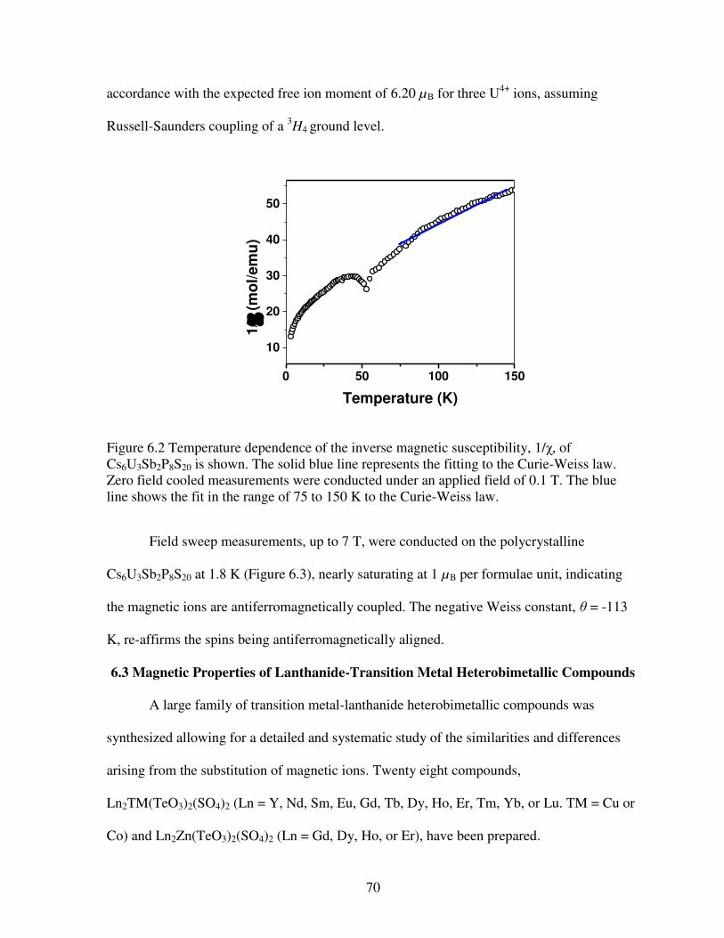
70

accordance with the expected free ion moment of 6.20 µB for three U4+ ions, assuming

Russell-Saunders coupling of a 3H4 ground level.

0 50 100 150

10

20

30

40

50

1/

(m

ol/

em

u)

Temperature (K)

Field sweep measurements, up to 7 T, were conducted on the polycrystalline

Cs6U3Sb2P8S20 at 1.8 K (Figure 6.3), nearly saturating at 1 µB per formulae unit, indicating

the magnetic ions are antiferromagnetically coupled. The negative Weiss constant, θ = -113

K, re-affirms the spins being antiferromagnetically aligned.

6.3 Magnetic Properties of Lanthanide-Transition Metal Heterobimetallic Compounds

A large family of transition metal-lanthanide heterobimetallic compounds was

synthesized allowing for a detailed and systematic study of the similarities and differences

arising from the substitution of magnetic ions. Twenty eight compounds,

Ln2TM(TeO3)2(SO4)2 (Ln = Y, Nd, Sm, Eu, Gd, Tb, Dy, Ho, Er, Tm, Yb, or Lu. TM = Cu or

Co) and Ln2Zn(TeO3)2(SO4)2 (Ln = Gd, Dy, Ho, or Er), have been prepared.

Figure 6.2 Temperature dependence of the inverse magnetic susceptibility, 1/χ, of Cs6U3Sb2P8S20 is shown. The solid blue line represents the fitting to the Curie-Weiss law. Zero field cooled measurements were conducted under an applied field of 0.1 T. The blue line shows the fit in the range of 75 to 150 K to the Curie-Weiss law.

71

0 20000 40000 60000 800000.0

0.2

0.4

0.6

0.8

1.0

M

( B

/Fo

rmu

lae U

nit)

Field (Oe)

They crystallize in the triclinic space group P1 with two different structural

topologies occurring owing to a reduction in the Ln3+ coordination number from eight to

seven due to the lanthanide contraction.

6.3.1 Synthesis and Structure

This large family of compounds was synthesized by combining Ln2O3, CuSO4, 1 M

H2SO4, with distilled water. These reagents were loaded into a 23 mL PTFE−lined autoclave

liner for the formation of Ln2Cu(TeO3)2(SO4)2 (Ln = Y, Nd, Sm, Eu, Gd, Dy, Ho, Er, Tm,

Yb, or Lu). To form the terbium analogue, Tb2Cu(TeO3)2(SO4)2, terbium metal (2 mmol_

was reacted with 1 M H2SO4 in an autoclave liner under room temperature. Then CuO and

TeO2 were loaded in the autoclave liner. The formation of the cobalt analogues required

CoO/CoCl2·6H2O/CoSO4·6H2O/CoAc2·4H2O instead of the copper while the zinc analogues

used Zn(O2CCH3)2(H2O)2 in its place. The autoclave was sealed and heated to 230 °C for 3

Figure 6.3 Field dependent Magnetization of Cs6U3Sb2P8S20 obtained at 1.8 K with an applied magnetic field ranging from 0 Oe up to 70 000 Oe.

72

days followed by slow cooling to room temperature at a rate of 5 °C/hr. The products were

washed with DI water to remove soluble solids, followed by rinsing with methanol.

The earlier lanthanides (Ln = Y, Nd, Sm, Eu, Gd, Tb, Dy, Ho, Er, and Tm)

crystalized in the topology depicted in Figure 6.4 while Figure 6.5 shows the topology for the

later lanthanides, Ln = Yb and Lu. Photographs depicting crystals of the cobalt analogues are

seen in Figure 6.6.

Figure 6.4 (a) View of the structure of Ln2TM(TeO3)2(SO4)2 (RE = Y, Nd, Sm, Eu, Gd, Tb, Dy, Ho, Er, or Tm. TM = Co, Zn, or Cu) extending down the a axis. (b) Representation of the trigonal dodecahedron coordination environment of Ln3+ ions. (c) [TM(TeO3)2(SO4)2]

6- unit. Ln3+ polyhedra are shown in cyan, TM2+ polyhedra in dark blue, TeO3

2- polyhedra in grey, SO4

2- tetrahedra in purple, and oxygen atoms in red.

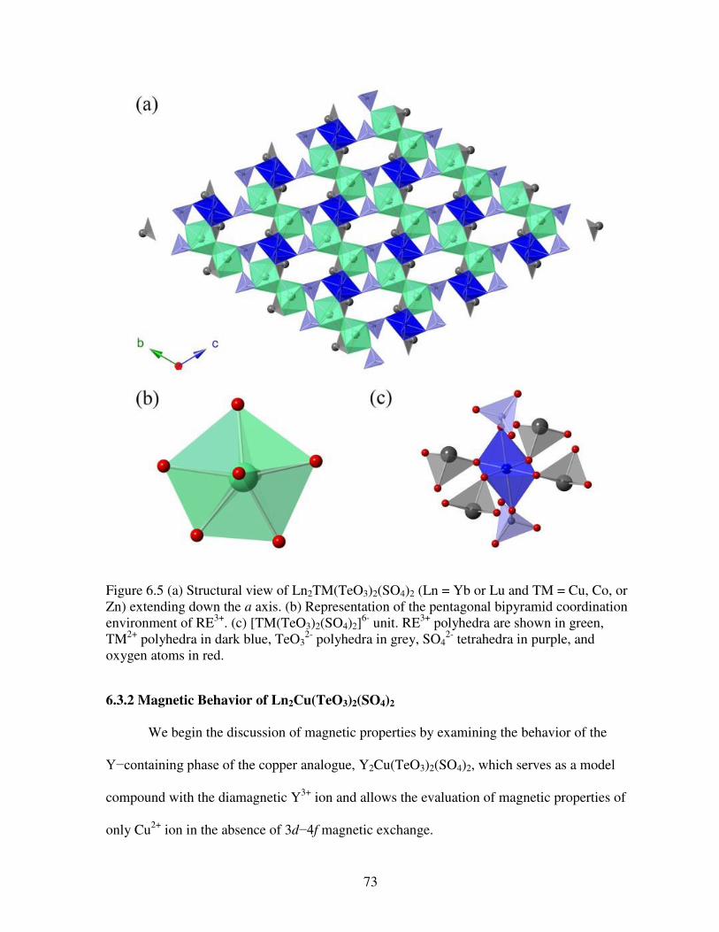
73

6.3.2 Magnetic Behavior of Ln2Cu(TeO3)2(SO4)2

We begin the discussion of magnetic properties by examining the behavior of the

Y−containing phase of the copper analogue, Y2Cu(TeO3)2(SO4)2, which serves as a model

compound with the diamagnetic Y3+ ion and allows the evaluation of magnetic properties of

only Cu2+ ion in the absence of 3d−4f magnetic exchange.

Figure 6.5 (a) Structural view of Ln2TM(TeO3)2(SO4)2 (Ln = Yb or Lu and TM = Cu, Co, or Zn) extending down the a axis. (b) Representation of the pentagonal bipyramid coordination environment of RE3+. (c) [TM(TeO3)2(SO4)2]

6- unit. RE3+ polyhedra are shown in green, TM2+ polyhedra in dark blue, TeO3

2- polyhedra in grey, SO42- tetrahedra in purple, and

oxygen atoms in red.

74

Above 50 K, the temperature (T) dependence of inverse susceptibility (–1) obeys the

modified Curie–Weiss law (Figure 6.7a, inset) is equal to 1.74 µB, which is very close to the

spin-only theoretical moment of the Cu2+ ion (1.73 µB for S = 1/2), consistent with the

diamagnetism of Y3+ ions as expected. The small negative Weiss temperature, θ = – 1.1(1) K,

indicates weak antiferromagnetic interactions between the Cu2+ ions, which also agrees with

the gradual drop in the χT value below 50 K (Figure 6.7b). An examination of the vs. T

dependence at low temperatures reveals a small hump around 15 K (Figure 6.7a), which

suggests an occurrence of an antiferromagnetic phase transition. As expected, the field

Figure 6.6 Photographs of crystals of Ln2Co(TeO3)2(SO4)2. From left to right and top to bottom can be seen the following analogues: Ln = Y, Nd, Sm, Eu, Gd, Tb, Dy, Ho, Er, Tm, Yb, and Lu.

75

dependence of magnetization is nearly linear (Figure 6.7c) and exhibits the maximum value

of 0.14 µB at 7 T, which is significantly lower than 1 µB expected for the S = 1/2 Cu2+ ion.

Thus, the weak magnetic exchange coupling between the Cu2+ ions results in

antiferromagnetic ordering in Y2Cu(TeO3)2(SO4)2 at TN = 12.5 K.

The Sm3+ and Eu3+ ions are well known to exhibit TIP effects due to the presence of

low-lying excited states. Consequently, the inverse susceptibility plots for both

Sm2Cu(TeO3)2(SO4)2 and Eu2Cu(TeO3)2(SO4)2 exhibit strong deviation from the Curie–

Weiss law. As the samples are cooled down, the depopulation of excited states leads to the

continuous decrease in χT that approaches zero at lower temperatures (Figures 6.8a, 6.8b).

Since the ground state of the Eu3+ ion is diamagnetic (7F0), one can expect the low-

temperature behavior of Eu2Cu(TeO3)2(SO4)2 to be similar to that of the isostructural Y-

containing analogue. Indeed, the peak observed in the magnetic susceptibility plot of the Eu-

containing sample (Figure 6.8d) indicates antiferromagnetic ordering of the Cu2+ moments at

TN = 15 K, close to the Néel temperature of Y2Cu(TeO3)2(SO4)2. In contrast, no signature of

Figure 6.7 Temperature dependence of magnetic susceptibility (a), inverse susceptibility (inset), and the T product (b) for Y2Cu(TeO3)2(SO4)2. (c) Field-dependent magnetization measured at 1.8 K. The solid red line in (a) shows the theoretical fit to the modified Curie-Weiss law.

76

magnetic phase transition was observed for Sm2Cu(TeO3)2(SO4)2 down to 1.8 K (Figure

6.8c). In the latter, besides the Cu2+–Cu2+ antiferromagnetic coupling, other interactions may

be present due to the paramagnetic ground state of the Sm3+ ions (6H5/2). We suggest that the

competition between different exchange pathways prevents the emergence of the magnetic

ordering for Sm2Cu(TeO3)2(SO4)2 in the investigated temperature range. Nevertheless, the

field-dependent magnetization measured at 1.8 K shows linear behavior with relatively small

maximum values for both Sm2Cu(TeO3)2(SO4)2 (0.31 B) and Eu2Cu(TeO3)2(SO4)2 (0.24 B)

(Figure 6.8e and 6.8f). This finding suggests the Sm-containing compound is close to

antiferromagnetic ordering that might occur at slightly lower temperatures than that available

in our experiment.

Figure 6.8 Temperature dependence of T (a and b), (c and d), and field dependence of magnetization at 1.8 K (e and f) for Sm2Cu(TeO3)2(SO4)2 and Eu2Cu(TeO3)2(SO4)2, respectively.

77

The Dy2Cu(TeO3)2(SO4)2 compound shows linear Curie-Weiss behavior in the χ–1 vs.

T data within the measured temperature range (Figure 6.9a, inset). To determine the effective

moment per Dy3+ ion, the contribution from the Cu2+ ion was subtracted from the total

moment. The effective moment obtained, 10.47 µB per Dy3+ ion, is in good agreement with

the theoretical value of 10.63 µB. The Weiss temperature is only slightly positive, θ = 0.09 K,

indicating very weak magnetic exchange coupling between the Cu2+ and Dy3+ moments. The

small dip followed by the sharp increase in the χT value around 15 K (Figure 6.9a) is

indicative of short-range antiferromagnetic correlations between the low Cu2+ magnetic

moments (S = 1/2) and the high Dy3+ magnetic moments (6H15/2, J = 15/2). The field-

dependent magnetization measured at 1.8 K shows the initial increase that follows the sum of

Brillouin functions for two Dy3+ and one Cu2+ ions in the absence of magnetic exchange

(Figure 6.9b). Nonetheless, at fields above 0.3 T the magnetization increases much slower

than expected from the Brillouin function, which can be explained by the population of low-

lying excited states. Both these observations are in agreement with the weak exchange

coupling between the Dy3+ and Cu2+ ions. No clear signature of magnetic ordering was

observed for this phase.

For Ln2Cu(TeO3)2(SO4)2 (Ln = Gd, Ho, Er, or Tm) the temperature dependence of χ–1

followed the Curie-Weiss law. The effective magnetic moments per Ln3+ ion matches well

with the theoretical values, while the negative Weiss temperatures indicate prevailing

antiferromagnetic interactions between the nearest-neighbor ions. The antiferromagnetic

exchange is also supported by the decrease in the χT value at lower temperatures and the

suppressed magnetization values as compared to the sum of Brillouin functions for two RE3+

and one Cu2+ ions at 1.8 K (Figure 6.10). A systematic increase in the strength of

78

antiferromagnetic exchange is observed as the RE3+ ionic radius decreases, as indicated by

pronouncedly more negative Weiss temperatures (-0.78 K for Gd3+, -3.5 K for Ho3+, -6.8 K

for Er3+, and -8.8 K for Tm3+).

It is difficult, however, to establish whether this effect stems from the stronger 3d−4f

exchange or just from the stronger antiferromagnetic interactions between the Cu2+ ions as

the lattice gets contracted (or from both). It was reported that the RE3+–Cu2+ interactions

favor ferromagnetic exchange for the late half of the lanthanide series.96, 116-118 Therefore, for

Ln2Cu(TeO3)2(SO4)2 (Ln = Gd, Ho, Er, or Tm), the Ln3+–Cu2+ coupling may be

ferromagnetic but overcome by antiferromagnetic Cu2+–Cu2+ and Ln3+–Ln3+ interactions.

The ytterbium compound behaves similarly to the four analogues just described,

despite its different structure. Both the χT vs. T and M vs. H plots support the presence of

antiferromagnetic exchange (Figure 6.11). The only notable difference is the significantly

more negative Weiss temperature, θ = – 44 K, which indicates that the antiferromangetic

interactions in Yb2Cu(TeO3)2(SO4)2 are stronger than those observed in the four compounds

Figure 6.9 Temperature dependence of T (a) and –1 (inset) and the field dependence of magnetization at 1.8 K (b) for Dy2Cu(TeO3)2(SO4)2. The solid red line in (a) shows the fit to the modified Curie-Weiss law, while the solid black line in (b) represents the magnetization calculated as the sum of Brillouin functions for two Dy3+ and one Cu2+ ions.

79

above. This increased antiferromagnetic exchange cannot be explained by the change in the

separation between the Cu2+ ions, as the nearest Cu-Cu distance in Yb2Cu(TeO3)2(SO4)2 is

significantly larger than those in the other Ln2Cu(TeO3)2(SO4)2 structures. On the other hand,

the RE-Cu distance in the former is the shortest in the series.

Thus, a more probable cause for the stronger antiferromagnetic interactions may be

the different structural type of Yb2Cu(TeO3)2(SO4)2 that promotes antiferromagnetic 3d−4f

coupling. Proving this assumption, however, is non-trivial due to the other competing

magnetic exchange pathways present in this crystal structure.

Figure 6.10 Temperature dependence of T and 1.8-K field dependence of magnetization (insets) for Ln2Cu(TeO3)2(SO4)2, where Ln = Gd (a), Ho (b), Er (c), and Tm (d). The solid lines in the insets represent the magnetization calculated as the sum of Brillouin functions for two Ln3+ and one Cu2+ ions.

80

6.3.3 Magnetic Behavior of Ln2Co(TeO3)2(SO4)2 and Ln2Zn(TeO3)2(SO4)2

To probe the contributions that arise from the magnetic interactions due purely to

copper without 3d/4f magnetic exchange, the diamagnetic Y and Lu−containing phases were

measured. Since the ground state of the Eu3+ ion is diamagnetic, 7F0, one can expect the low-

temperature behavior of Eu2Co(TeO3)2(SO4)2 to be similar to that of Y2Co(TeO3)2(SO4)2.

The temperature dependence of the magnetic susceptibility data for Y2Co(TeO3)2(SO4)2,

Eu2Co(TeO3)2(SO4)2, and Lu2Co(TeO3)2(SO4)2 measured under an applied field of 1000 Oe

are shown in Figures 6.12a and 6.12e, respectively. An examination of the vs. T

dependence at low temperatures reveals a Curie tail around 3 K for these three compounds.

This feature is attributed to the intrinsic anisotropy of the Co2+ ions since it is unlikely that all

of these independently prepared complexes would contain similar impurities. The magnetic

Figure 6.11 Temperature dependence of T and 1.8-K field dependence of magnetization (inset) for Yb2Cu(TeO3)2(SO4)2. The solid line represents the magnetization calculated as the sum of Brillouin functions for two Ln3+ and one Cu2+ ions.

81

anisotropy arises from the orbital momentum contributions of the spin-orbit coupled Co2+

unpaired electrons within the non-spherical octahedral crystal field environment.

The similarities in magnetic susceptibility between Y2Co(TeO3)2(SO4)2 and

Eu2Co(TeO3)2(SO4)2 are not surprising owing to the diamagnetic ground states of Y and Eu

within the same structure type. Although Lu2Co(TeO3)2(SO4)2 has a different structure

compared to the early lanthanide compounds, similar behavior is observed that can be

attributed to the comparable Co2+···Co2+ distances between the nearest spin carriers compared

with that of Eu2Co(TeO3)2(SO4)2, Table 6.1.

Ln Ln3+−Ln3+ (Å)

Ln3+−Co2+ (Å)

Co2+−Co2+ (Å)

Y 3.7990 (9) 3.4260 (5) 5.2216(4) Nd 3.9393(6) 3.4815(5) 5.3553(7) Sm 3.8904 (7) 3.4631 (4) 5.3120(4) Eu 3.873(1) 3.462(1) 5.302(2) Gd 3.8653(6) 3.4593(5) 5.2897(7) Tb 3.8188(1) 3.4410(4) 5.2762(7) Dy 3.8259(6) 3.4400(4) 5.2609(4) Ho 3.811(1) 3.430(1) 5.245(1) Er 3.7906(6) 3.4183(4) 5.2334(2) Yb 3.7526(6) 3.3280(4) 5.4004(6) Lu 3.7393(5) 3.3178(3) 5.3893(5)

Above 100 K, the temperature dependence of inverse susceptibility (–1) of

Y2Co(TeO3)2(SO4)2 and Lu2Co(TeO3)2(SO4)2 obeys the Curie–Weiss law, Figures 6.12b and

6.12f, inset. Negative Weiss temperatures result from the fittings, θ = – 17.1(4) K and –

3.1(5) K, indicate weak antiferromagnetic interactions occurring between the nearest-

neighbor Co2+ ions that also agrees with the gradual drop in the χT value below 100 K

Table 6.1 The closest Ln3+···Ln3+, Ln3+

···Co2+, and Co2+···Co2+ bond distances in

Ln2Co(TeO3)2(SO4)2 are shown for each of the measured lanthanides.

82

(Figure 6.12b and 6.12f). The Eu3+ ion is known to show Van Vleck paramagnetism because

of the presence of low-lying excited states.119 Consequently, Eu2Cu(TeO3)2(SO4)2 exhibits

strong deviations from the Curie–Weiss law. As Eu2Co(TeO3)2(SO4)2 is cooled, the

depopulation of excited states leads to the sharper decrease in χT than those of

Y2Co(TeO3)2(SO4)2 and Lu2Co(TeO3)2(SO4)2 (Figures 6.12b and 6.12f).

Nd2Co(TeO3)2(SO4)2 behaves as a typical paramagnetic material with

antiferromagnetic interactions as the plots of χ, χT, and 1/χ versus temperature show in

Figures 6.13a, 6.13b, and 6.13a (inlet), respectively. The χT value decreases exponentially

with decreasing temperature, attributed to antiferromagnetic interactions. The observed value

of eff at 300 K is 7.20 µB and is relatively close to the calculated value of 7.30 µB expected

for two Nd3+ and one Co2+ ion for the corresponding ground states 4I9/2 and 2F9/2,

respectively. The slight difference of 0.1 µB is attributed to nearest-neighbor

antiferromagnetic interactions (θ = -32.6 K) which was obtained via a Curie-Weiss fitting to

the χ-1 plot between 75 K and 300 K.

The gadolinium, dysprosium and terbium analogues µ eff values that match well with

the theoretical values for two Ln3+ and one Co2+ vide infra Table 6.1. To determine the

effective magnetic moments, the temperature dependence of χ–1 was least-squares fit to the

Curie-Weiss law in the 50–300 K range (Figure 6.14a, Figure 6.14c, and Figure 6.14e).

The negative Weiss temperatures of -2.14(8) K for the Gd and -2.94(4) K for the Dy

compounds may indicate weak antiferromagnetic interactions between the nearest-neighbor

ions.

83

Figure 6.12 Temperature dependence of magnetic susceptibility , T product with inverse susceptibility as an inset for Y2Co(TeO3)2(SO4)2 (a, b), Eu2Co(TeO3)2(SO4)2 (c, d), and Lu2Co(TeO3)2(SO4)2 (e, f). The solid red lines in the insets show the fitting to the Curie-Weiss law in terms of inverse susceptibility.

84

The Tb analogue exhibits a positive Weiss temperature of 1.8(1) K, suggesting a

weak ferromagnetic relationship between closest-neighbor spins above 50 K. It is difficult,

however, to establish whether this divergence stems from the stronger 3d/4f exchange or just

from the interactions between Ln3+ ions (or from the combination of both).

Magnetic behavior studies of Ln2Zn(TeO3)2(SO4)2 (Ln = Gd and Dy) suggests

ferromagnetic correlations between the lanthanide centers below 25 K. These results match

well with the χT values of Gd and Dy analogues (Figure 6.14b and Figure 6.14f,

respectively), which decrease with decreasing temperature followed by the sharp increase in

the χT values around 25 K. Nonetheless, at temperatures below 3 K, the χT values decrease

abruptly, which can be attributed to the Co2+ ions. Tb2Zn(TeO3)2(SO4)2 was not included in

this study because the same synthetic method failed to generate the isotypic analogue,

however, it was reported that the Tb3+···Tb3+ interactions favor ferromagnetic exchange.120, 121

In addition, the Tb analogue displays the same increase in χT around 25 K as observed for

the Gd and Dy analogues, Figure 6.14d. The Tb analogue differs slightly in that it display

Figure 6.13 Temperature dependence of magnetic (a) magnetic susceptibility, , inverse magnetic susceptibility (inset), and the (b) T product for Nd2Co(TeO3)2(SO4)2.

85

slight ferromagnetic interactions throughout the measured temperature range which is clearly

seen in the increasing χT v T susceptibility (Figure 6.14d). Therefore, for

Ln2Co(TeO3)2(SO4)2 (Ln = Gd, Tb, and Dy), Ln3+···Ln3+ exhibit weak ferromagnetic

correlations that are overcome by weak Co2+···Co2+ interactions at 3 K. The different

magnitudes of these two interactions results in diverse magnetic behavior in the Gd, Dy, and

Tb phases.

Figure 6.14 Temperature dependence of magnetic susceptibility , inverse susceptibility (inset), and the T product for (a,b) Gd2Co(TeO3)2(SO4)2, (c,d) Tb2Co(TeO3)2(SO4)2, (e,f) Dy2Co(TeO3)2(SO4)2.

86

The remaining zinc containing phases allow for the evaluation of magnetic properties

arising due to Ho3+/Er3+ ions in the absence of any 3d/4f magnetic exchange. These

compounds show typical Curie-Weiss behavior in the χ–1 vs. T data. The Weiss temperatures

are found to be 13.6(2) K and 9.7(5) K for Ho2Zn(TeO3)2(SO4)2 and Er2Zn(TeO3)2(SO4)2,

respectively; indicating ferromagnetic interactions between nearest-neighbor Ln3+ ions. The

ferromagnetic exchange is also supported by the increase in the χT value with decreasing

temperature from 300 K to 5 K for the holmium analogue (Figure 6.15b) and 300 K to 15 K

for erbium (Figure 6.15d). Thereafter the χT values drops abruptly near 5 K for Ho and 15 K

for the Er analogues, respectively, which could be attributed to the depopulation of the mJ

levels of the Ho3+ and Er3+ ions at low temperatures.77

As shown in Figure 6.15a and Figure 6.15c, Ho2Co(TeO3)2(SO4)2 and

Er2Co(TeO3)2(SO4)2 follow the Curie-Weiss law with slightly negative Weiss temperatures (-

1.8(2) K for Ho and -4.8(2) K for the Er phase). The effective moment is equal to 16.45 µB

for Ho2Co(TeO3)2(SO4)2 and 14.90 µB for Er2Co(TeO3)2(SO4)2, which are slightly higher but

within reasonable agreement with the theoretical values of 15.87 µB and 14.53 µB,

respectively. The field-dependent magnetization measured at 1.8 K shows suppressed

magnetization values as compared to the sum of Brillouin functions for two Ln3+ and one

Co2+ ions in the absence of magnetic exchange. Both the decreasing χT upon cooling and

suppressed magnetization relative to paramagnetic ions suggest weak antiferromagnetic

interactions between the Ln3+ and Co2+ ions as well as between Co2+· · ·Co2+ overshadowing

the weak ferromagnetic correlations between Ln3+ ions. No clear signature of magnetic

ordering was observed for these phases.

87

Lastly, Yb2Co(TeO3)2(SO4)2, which is isomorphous with Lu2Co(TeO3)2(SO4)2

displays antiferromagnetic exchange interactions with a negative Weiss temperature, θ = – 44

K as seen in the 1/χ vs. T (Figure 6.16a inlet) and χT vs. T (Figure 6.16b). The field-

dependent magnetization measured at 1.8 K shows linear behavior with a very small

maximum value of 0.26 B. This further enforces that the Yb-containing compound has

antiferromagnetic interactions.

Figure 6.15 Temperature dependence of magnetic susceptibility, , inverse susceptibility (inset), and the T product for (a,b) Ho2Co(TeO3)2(SO4)2 and Ho2Zn(TeO3)2(SO4)2. (c,d) Er2Co(TeO3)2(SO4)2 and Er2Zn(TeO3)2(SO4)2.

88

To probe the cobalt ground terms, the Ln3+ cation in Ln2Co(TeO3)2(SO4)2 must be

diamagnetic, allowing the field dependence magnetization at 1.8 K to investigate the cobalt

magnetic behavior without 3d4f magnetic exchange. Theories of the paramagnetic properties

of Co2+ ions have been discussed in great detail where anisotropy and spin-orbit coupling

play a large role and must be accounted for in order to understand experimental results.33

Data for the yttrium analogue are provided in Figure 6.17a and show a saturation of

magnetization at approximately 2.5 μB. The calculated effective magnetic moments are much

higher, even excluding orbital contributions, a high-spin Co2+ ion yields 3.87 μB (S = 3/2)

while accounting for orbital contributions yields a magnetic moment of 5.20 μB (S = 3/2 and

L = 3). Most observed values of Co2+ ions in analogues environments typically saturate

between 4.5 μB ~ 5.2 μB as expected,32 although some complexes reported by Sacco and

Cotton saturate much lower, for instance; 1.82 μB, 1.89 μB, and 1.92 μB for

[Co(CH3NC)4][CdX4] (X = Br, I), [Co(MeNC)4X2 (X = Cl, Br, I)], and [Co

darsine3](CLO4)2, respectively.33 The low magnetic saturation values exhibited by

Figure 6.16 (a) Temperature dependence of magnetic susceptibility, , inverse susceptibility, -1, (inset), and (b)the T product for Yb2Co(TeO3)2(SO4)2.

89

Ln2Co(TeO3)2(SO4)2 are thus not surprising considering the aforementioned Co2+ ions in

octahedral environments that saturate far below the theoretical values calculated from Eq. 6.1

for non-interacting Co2+ ions.

√ ( ) (6.1)

The Gd3+, Tb3+, and Dy3+ cases will be briefly compared owing to the diversity

displayed by their field-dependent magnetizations. Gd3+ has the largest spin moment (S =

7/2) and possesses electronically isotropic f orbitals. Consequently, the magnetization of

Gd2Co(TeO3)2(SO4)2 is in good agreement with the sum of Brillouin functions for two free

Gd3+ ions and one Co2+ ion (Figure 6.17b) until higher applied fields after which it saturates

below the expected value due to effects by the Co2+ ion. The Tb analogue exceeds the

theoretical Brillouin function up to 0.5 T, which can be explained by ferromagnetic

correlations, and then saturates at a lower value than the calculated Brillouin function due to

orbital contributions from the Tb3+ ions (L = 3) and Co2+ effects that are shown in Figure

6.17c. The Dy analogue (Figure 6.17d) tracks well with the Brillouin function up to 0.3 T and

then deviates because of the population of low-lying excited states as observed for our

previously reported dysprosium analogue.103

6.4 Antiferromagnetic Ordering in Cu3(TeO4)(SO4)•H2O

Cu3(TeO4)(SO4)·H2O crystallized as a side product from the preparation of

Ln2Cu(TeO3)2(SO4)2 among other copper tellurite sulfate reactions. Single-crystal X-ray

diffraction studies reveal that Cu3(TeO4)(SO4)·H2O crystallizes in an orthorhombic space

group Pnma with a three-dimensional (3D) framework. The main feature of

90

Cu3(TeO4)(SO4)·H2O is the channels that extend down the b axis (Figure 6.18a). Another

view of the structure is shown in Figure 6.18b. The Cu2+ cations, TeO44−, and SO4

2− anions

do not fill all of the space in the crystals, and as a result of this architecture, a system of

channels with voids in the structure is observed.

These channels have dimensions of 5 Å × 7 Å and one crystallographically

independent water molecule resides in the channels. The framework of the channels is

composed of two crystallographically unique Cu2+ cations, one TeO44− anion, and one SO4

2−

Figure 6.17 Magnetization plots of (a) Y2Co(TeO3)2(SO4)2, (b) Gd2Co(TeO3)2(SO4)2, (c) Tb2Co(TeO3)2(SO4)2, (d) Dy2Co(TeO3)2(SO4)2. The solid red line represents the theoretical Brillouin fitting which accounts for non-interacting magnetic spins with spin orbit coupling.

91

ion. Both Cu2+ ions feature a square planar coordination with Cu-O distances ranging from

1.91(2) to 2.00(2) Å. Examination of the magnetic susceptibility as a function of temperature

reveals an anomalous peak around 72 K, which decreases toward the background, as

expected for an antiferromagnetic transition at 72 K, as seen in Figure 6.19a. On further

cooling, a curie tail is evidenced below 25 K arising from paramagnetic contributions which

may be attributed to Cu(1) which has increased bond distances relative to the Cu(2) ions.

Figure 6.18 (a) View of the structure of Cu3(TeO4)(SO4)·H2O down the b axis; (b) View of the structure of Cu3(TeO4)(SO4)·H2O down the c axis. Copper polyhedra are shown in green, tellurite polyhedra in cyan, and sulfate anions in grey.

92

Figure 6.19 (a) Temperature dependence of magnetic susceptibility χ at 1000 Oe and 100 Oe (inset) for Cu3(TeO3)(SO4)(H2O)2; (b) field dependence of magnetization at 1.8 K, 50 K, 70 K, and 80 K for Cu3(TeO3)(SO4)(H2O)2, (c) A ball and stick model of the Cu2+ ions showing the Cu(1) ions in light green and the Cu(2) ions in dark green.

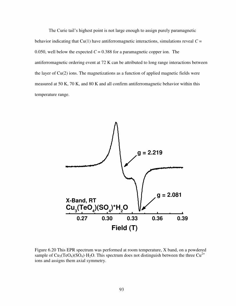
93

The Curie tail’s highest point is not large enough to assign purely paramagnetic

behavior indicating that Cu(1) have antiferromagnetic interactions, simulations reveal C =

0.050, well below the expected C = 0.388 for a paramagnetic copper ion. The

antiferromagnetic ordering event at 72 K can be attributed to long range interactions between

the layer of Cu(2) ions. The magnetizations as a function of applied magnetic fields were

measured at 50 K, 70 K, and 80 K and all confirm antiferromagnetic behavior within this

temperature range.

0.27 0.30 0.33 0.36 0.39

g = 2.081X-Band, RT

Field (T)

Cu3(TeO

4)(SO

4)*H

2O

g = 2.219

Figure 6.20 This EPR spectrum was performed at room temperature, X band, on a powdered sample of Cu3(TeO4)(SO4)·H2O. This spectrum does not distinguish between the three Cu2+ ions and assigns them axial symmetry.

94

To further elucidate the nature of the magnetic coupling between the copper ions in

Cu3(TeO3)(SO4)(H2O)2, EPR measurements were performed at room temperature beginning

with measurements using a 9 GHz source, as seen in Figure 6.20.

When measured using 34 GHz source, the three copper ions remain magnetically

equivalent at room temperature. The X band spectrum does not distinguish the various

copper ions and assigns to them an axial symmetry due to the square planar geometry

surrounding the Cu2+ ions.

0.9 1.0 1.1 1.2 1.3 1.4

g = 2.400g = 2.262

g = 2.089

Field (T)

Field (T)Field (T)

Cu3(TeO

4)(SO

4)*H

2O

Q-Band, RT

Figure 6.21 This figure shows the Q band EPR spectra of powdered Cu3(TeO4)(SO4)·H2O. All three Cu2+ ions have similar local symmetry, distorted square planar, such that the three principal magnetic axes are distinctly different. The value of 2.089 corresponds to the out of plane orientation, with dz

2 as the ground state.

95

The magnetic susceptibility data and crystal structure show two crystallographically

and magnetically unique Cu2+ ions which should be distinguishable via EPR, and thus higher

frequencies were measured in an attempt to resolve them.

Weak spin exchange obliterates the expected four-line hyperfine structure expected

from the Cu2+ ions. The local symmetry is square planer but distorted, thus the three principal

axes are different as seen in Figure 6.21. This slight distortion was not observable in the X

band measurements due to the Q band g = 2.400 being buried within the left X band peak. It

6.5 7.0 7.5 8.0 8.5

240 GHzCu

3(TeO

4)(SO

4)*H

2O

5 K

Field (T)

2.46972.2537

2.2449

2.1357

2.0697

2.40092.2565

2.2479 2.0984

2.0731

1234

5

290 K

Figure 6.22 HFEPR spectra are shown for powdered Cu3(TeO4)(SO4)·H2O at room temperature and 5 K using 240 GHz. Peaks are labeled from right to left with a vertical dashed blue line showing the peak shift over the measured temperature range. The black and red values represent the corresponding g tensors for the respective peaks.

96

was assumed that the exchange becomes stronger than the thermal energy at about 72 K at

which point the Cu3(TeO4)(SO4)·H2O lattice experiences antiferromagnetic ordering but

variable temperature measurements performed at 240 GHz show no such deviations.

To probe the system further in an attempt to differentiate the two crystallographically

unique Cu2+ ions, HFEPR measurements were necessary. These measurements do indeed

separate the two crystallographically unique Cu2+ ions, Cu(1) and Cu(2), as well as the two

different Cu(2) ions, which are distinctly observed in Figure 6.22. The peaks labeled as 3 and

4 in Figure 6.22 represent the gz tensor components of the two Cu(2) ions while gz of Cu(1)

is represented by peak 5. Peak 2 in this figure is a mixture of the gy components for the

various copper ions with peak 1 being the gx tensor. The HFEPR spectrum at 5 K assigns the

ground states of the Cu2+ ions to be in the dx2

- y2 orbital.4

6.5 Conclusions

Cs6U3Sb2P8S32 is a rare example of an ordered quinary compound which is difficult to

find due to the complexity of finding five different elements that are compatible with one

another in a single compound. The U4+ centers in Cs6U3Sb2P8S32 form trimers that are

antiferromagnetically coupled causing a spin frustrated system, revealing a well-defined peak

at 53 K.

Y2Cu(TeO3)2(SO4)2 and Eu2Cu(TeO3)2(SO4)2 display antiferromagnetic ordering at

12.5 K and 15 K, respectively, owing to the magnetic exchange between Cu2+ moments. No

magnetic phase transition was observed in the other copper analogues. The lack of magnetic

ordering is attributed to the competing magnetic interactions caused by the presence of

paramagnetic Ln3+ ions. Magnetic susceptibility studies on compounds using diamagnetic

lanthanides, and lanthanide-like ions, as Ln surrogates in Ln2Co(TeO3)2(SO4)2 suggest that

97

antiferromagnetic interactions occur between the Co2+ ions. In general, the experimental

results match well with the computational results for two paramagnetic lanthanide ions with a

high-spin cobalt ion.

The Weiss constants shed light on how the nearest neighbors are interacting. While

structural characterizations yield a deviation in structure between thulium and ytterbium, no

such deviation is evident in terms of magnetic properties, further hinting to paramagnetic

behavior of the magnetic ions. By substituting in diamagnetic ions for Ln3+ in

Ln2Co(TeO3)2(SO4)2, we observe antiferromagnetic correlations between cobalt ions.

Tb2Co(TeO3)2(SO4)2 displays ferromagnetic correlations at higher temperatures while the rest

are antiferromagnetic. Careful analysis of the zinc analogues, Ln = Gd, Dy, Ho, and Er yield

ferromagnetic interactions occurring between the lanthanide ions that are cloaked in

Ho2Co(TeO3)2(SO4)2 and Er2Co(TeO3)2(SO4)2. No long-range magnetic ordering is observed

for these compounds, but unlike the copper analogues, a wide range of ferromagnetic and

antiferromagnetic interactions occur between the Ln3+ and the Co2+ cations, with several

compounds exhibiting short-range magnetic correlations below 25 K.

Many times, side products in reactions are overlooked, luckily for us we found

Cu3(TeO4)(SO4)·H2O as an impurity several times and were able to isolate enough for

magnetic studies. Two distinct Cu2+ ions were found via magnetic susceptibility

measurements which reveal an antiferromagnetic ordering event at 72 K with a large

paramagnetic Curie tail below 25 K. HFEPR was able to clearly distinguish the three various

copper centers magnetically and revealed the ground state to be in the dx2

- y2 orbital at 5 K.

98

CHAPTER 7

SUMMARY AND ANALYSIS

This dissertation covers merely a few projects that I have found to be noteworthy and

that represent a wide variety of magnetic properties we have discovered to be intrinsic to

various novel materials that we were able to synthesize and characterize.

The neptunium iodate and selenite compounds included within were discovered as

novel materials for us to analyze and to probe further into the realm of actinide magnetism.

Three of these neptunium compounds were found to have soft ferromagnetic ordering while

the iodates also had a frequency dependent component to their magnetic susceptibility which

we assigned to spin glass behavior. This field is yet in its infancy and is proving to be quite

difficult to model due to safety precautions and scarcity of material as well as large

contributions from spin-orbit coupling, low lying excited states, relativistic effects, and

various other phenomenon, but rather rewarding with a wide variety of magnetic,

metallurgic, optical, and other properties worth further investigating and then optimizing.

These investigations will lead to improved nuclear waste remediation, novel technologies,

and improving available ones.

In terms of the lanthanides, various families of compounds with variable metal

centers were found to have a large diversity of magnetic properties. These compounds were

excellent for investigating magnetically and comparing the magnetic behavior that arises due

to minute changes in bond distances, ligand geometries, and the number of unpaired

electrons across the series. Particularly, two compounds both of which contain gadolinium

and copper are shown to be magnetically quite different. One compound obeys the expected

Cure-Weiss behavior while the other appears to deviate drastically which we found to be due

99

to a greater amount of magnetic exchange. These studies shed light on the tunability of

magnetic properties of materials containing lanthanide ions, which are easily

interchangeable, due to similar ionic radii and formal charge.

By using magnetic susceptibility as the only means of probing the magnetic behavior

of a system, limitations are intrinsic in terms of the magnetic information that can be

obtained about a system. This is primarily due to these measurements being bulk techniques.

By using electron paramagnetic resonance (EPR) as a complimentary technique, especially at

higher magnetic fields, we can probe single electrons to model magnetic behavior more

accurately. With these EPR measurements, we observed magnetically distinct copper ions, in

a compound containing three Cu2+ ions in its unit cell, and determined what was causing the

deviations from the Curie-Weiss law in the above mentioned gadolinium compound. These

techniques coupled together allow the demystification of the magnetic behavior of novel

materials and have been informative tools throughout my research experience.

100

APPENDIX A

COPYRIGHT INFORMATION

Permission 1:

101

Permission 2:

102

Permission 3:

103

Permission 4:

104

BIBLIOGRAPHY

1. Cotton, S., Lanthanide and Actinide Chemistry. Vol. 16. 2006: Wiley. 263. 2. Edelstein, N.M.; J. Fuger; L.R. Morss, The Chemistry of the Actinide and

Transactinide Elements. 2010: Springer. 3. Clark, D.L.; D.E. Hobart; M.P. Neu, Chem. Rev., 1995, 95 (1), 25-48. 4. Weil, J.A.; J.R. Bolton, Electron Paramagnetic Resonance. 2006, John Wiley &

Sons, Inc. 5. Moiseev, I.V.; A.Y. Kuperman; N.N. Borodina; V.A. Vinokurov, Radiokhimiya,

1975, 17, 189-95. 6. Shilov, V.P., Radiokhimiya, 1980, 5, 727-32. 7. Sarsfield, M.J.; R.J. Taylor; C.J. Maher, Radiochim. Acta, 2007, 95, 677-682. 8. Wang, S.; E.M. Villa; J. Diwu; E.V. Alekseev; W. Depmeier; T.E. Albrecht-Schmitt,

Inorg. Chem., 2011, 50, 2527-33. 9. Meredith, N.A.; M.J. Polinski; J. Lin; A. Simonetti; T.E. Albrecht-Schmitt, Inorg.

Chem., 2012, 51 (20), 10480-10482. 10. Diwu, J.; S. Wang; Z. Liao; P.C. Burns; T.E. Albrecht-Schmitt, Inorg. Chem., 2010,

49, 10074-80. 11. Villa, E.M.; S. Wang; E.V. Alekseev; W. Depmeier; T.E. Albrecht-Schmitt, Eur. J.

Inorg. Chem., 2011, 2011, 3749-3754. 12. Bray, T.H.; A.-G.D. Nelson; G.B. Jin; R.G. Haire; T.E. Albrecht-Schmitt, Inorg.

Chem., 2007, 46 (26), 10959-10961. 13. Gal, J.; M. Kroup; Z. Hadari, Solid State Commun., 1976, 19, 73-4. 14. Jin, G.-B.; S. Skanthakumar; R.G. Haire; L. Soderholm; J.A. Ibers, Inorg. Chem.,

2011, 50, 1084-1088. 15. Vlaisavljevich, B.; P. Miró; D. Ma; G.E. Sigmon; P.C. Burns; C.J. Cramer; L.

Gagliardi, Chem. Eur. J, 2013, 19 (9), 2937-2941. 16. Shannon, R., Acta Crystallogr. Sect. A: Found. Crystallogr., 1976, 32 (5), 751-767. 17. Peng, J.B.; Q.C. Zhang; X.J. Kong; Y.Z. Zheng; Y.P. Ren; L.S. Long; R.B. Huang;

L.S. Zheng; Z. Zheng, J. Am. Chem. Soc., 2012, 134, 3314.

105

18. Wang, C.M.; Y.Y. Wu; C.H. Hou; C.C. Chen; K.H. Lii, Inorg. Chem., 2009, 48, 1519.

19. Mishra, A.; A.J. Tasiopoulos; W. Wernsdorfer; K.A. Abboud; G. Christou, Inorg.

Chem., 2007, 46 (8), 3105-3115. 20. Wang, Y.; M. Fang; Y. Li; J. Liang; W. Shi; J. Chen; P. Cheng, Int. J. Hydrogen

Energy, 2010, 35, 8166. 21. Sankar, S.G.; V.U.S. Rao; E. Segal; W.E. Wallace; W.G.D. Frederick; H.J. Garrett,

Phys. Rev. B, 1975, 11 (1), 435-439. 22. Schelter, E.J.; D.E. Morris; B.L. Scott; J.D. Thompson; J.L. Kiplinger, Inorg. Chem.,

2007, 46 (14), 5528-5536. 23. Richardson, R.P.; J.B. Gruber, J. Chem. Phys., 1972, 56 (1), 256-260. 24. Weil, J.A.; J.R. Bolton, Electron Paramagnetic Resonance. 2006, John Wiley &

Sons, Inc. 36-57. 25. Mishra, A.; W. Wernsdorfer; S. Parsons; G. Christou; E.K. Brechin, Chem. Commun.,

2005, 2086. 26. Lin, J.; J.N. Cross; J. Diwu; M.J. Polinski; E.M. Villa; T.E. Albrecht-Schmitt, Inorg.

Chem., 2012, 51, 11949. 27. Magnani, N.; C. Apostolidis; A. Morgenstern; E. Colineau; J.-C. Griveauν H. Bolvin ν

O. Walter; R. Caciuffo, Angew. Chem. Int. Ed., 2011, 50 (7), 1696-1698. 28. Neidig, M.L.; D.L. Clark; R.L. Martin, Coord. Chem. Rev., 2013, 257 (2), 394-406. 29. Palenik, G., J. Inorg. Chem., 1997, 36, 4888. 30. Mills, D.P.; F. Moro; J. Mcmaster; J. Van Slageren; W. Lewis; A.J. Blake; S.T.

Liddle, Nat. Chem., 2011, 3 (6), 454-460. 31. Mishra, A.; W. Wernsdorfer; K.A. Abboud; G. Christou, J. Am. Chem. Soc., 2004,

126, 15648. 32. Wemple, M.W.; H.L. Tsai; S. Wang; J.P. Claude; W.E. Streib; J.C. Huffman; D.N.

Hendrickson; G. Christou, Inorg. Chem., 1996, 35, 6450. 33. Wernsdorfer, W., Adv. Chem. Phys., 2001, 118, 99. 34. Bain, G.A.; J.F. Berry, J. Chem. Educ., 2008, 85, 532-536.

106

35. King, D.M.; F. Tuna; J. Mcmaster; W. Lewis; A.J. Blake; E.J.L. Mcinnes; S.T. Liddle, Angew. Chem. Int. Ed., 2013, 52 (18), 4921-4924.

36. Okane, T.; T. Ohkochi; T. Inami; Y. Takeda; S.I. Fujimori; N. Kawamura; M. Suzuki;

S. Tsutsui; H. Yamagami; A. Fujimori; A. Tanaka; D. Aoki; Y. Homma; Y. Shiokawaν E. Yamamotoν Y. Hagaν A. Nakamuraν Y. Ōnuki, Phys Rev B, 2009, 80 (10), 104419.

37. Bray, T.H.; S. Skanthakumar; L. Soderholm; R.E. Sykora; R.G. Haire; T.E. Albrecht-

Schmitt, J. Solid State Chem., 2008, 181, 493-498. 38. Mao, J.-G.; H.-L. Jiang; F. Kong, Inorg. Chem., 2008, 47 (19), 8498-8510. 39. Jiang, H.-L.; Z. Xie; J.-G. Mao, Inorg. Chem., 2007, 46 (16), 6495-6501. 40. Ling, J.; T.E. Albrecht-Schmitt, Inorg. Chem., 2007, 46, 5686-90. 41. Lee, D.W.; K.M. Ok, Inorg. Chem., 2013(52), 5176–5184. 42. Almond, P.M.; R.E. Sykora; S. Skanthakumar; L. Soderholm; T.E. Albrecht-Schmitt,

Inorg. Chem., 2004, 43 (3), 958-963. 43. Jin, G.B.; S. Skanthakumar; L. Soderholm, Inorg. Chem., 2012, 51 (5), 3220-3230. 44. Wang, S.; E.V. Alekseev; W. Depmeier; T.E. Albrecht-Schmitt, Chem. Commun.,

2010, 46, 3955-7. 45. Wang, S.; E.V. Alekseev; H.M. Miller; W. Depmeier; T.E. Albrecht-Schmitt, Inorg.

Chem., 2010, 49, 9755-7. 46. Bray, T.H.; J. Ling; E.S. Choi; J.S. Brooks; J.V. Beitz; R.E. Sykora; R.G. Haire; D.M.

Stanbury; T.E. Albrecht-Schmitt, Inorg. Chem., 2007, 46, 3663-3668. 47. Gruen, D.M.; C.A. Hutchison, Jr., J. Chem. Phys., 1954, 22, 386-93. 48. Barbieri, G.A.; J. Calzolari, Berichte der deutschen chemischen Gesellschaft, 1910,

43 (2), 2214-2216. 49. Gorden, A.E.V.; J. Xu; K.N. Raymond; P. Durbin, Chem. Rev., 2003, 103 (11), 4207-

4282. 50. Hagan, P.G.; J.M. Cleveland, J. Inorg. Nucl. Chem., 1966, 28 (12), 2905-2909. 51. Kepert, D.L., Prog. Inorg. Chem. 2007, John Wiley & Sons, Inc. 179-249.

107

52. Villa, E.M.; S. Wang; E.V. Alekseev; W. Depmeier; T.E. Albrecht-Schmitt, Eur. J.

Inorg. Chem., 2011, 2011 (25), 3749-3754. 53. Tian, G.; L. Rao; A. Oliver, Chem. Commun., 2007(40), 4119-4121. 54. Fedoseev, A.M.; A.V. Gogolev; V.P. Shilov, Radiochemistry, 2013, 55 (2), 155-157. 55. Wang, S.A.; E.M. Villa; J.A. Diwu; E.V. Alekseev; W. Depmeier; T.E. Albrecht-

Schmitt, Inorg. Chem., 2011, 50 (6), 2527-2533. 56. Liu, G.; S. Wang; T.E. Albrecht-Schmitt; M.P. Wilkerson, J. Phys. Chem. A, 2012,

116 (32), 8297-8302. 57. Sessoli, R.; H.L. Ysai; A.R. Schake; S. Wang; J.B. Vincent; K. Folting; D. Gatteschi;

G. Christou; D.N. Hendrickson, J. Am. Chem. Soc., 1993, 115, 1804. 58. Sessoli, R.; H.L. Tsai; A.R. Schake; S. Wang; J.B. Vincent; K. Folting; D. Gatteschi;

G. Christou; D.N. Hendrickson, J. Am. Chem. Soc., 1993, 115 (5), 1804-1816. 59. Seth, M.; M. Dolg; P. Fulde; P. Schwerdtfeger, J. Am. Chem. Soc., 1995, 117 (24),

6597-6598. 60. Magnani, N.; E. Colineau; R. Eloirdi; J.C. Griveau; R. Caciuffo; S.M. Cornet; I. May;

C.A. Sharrad; D. Collison; R.E.P. Winpenny, Phys. Rev. Lett., 2010, 104, 197202/1-197202/4.

61. Rinehart, J.D.; J.R. Long, Chem. Sci., 2011, 2, 2078. 62. Ruiz, J.; G. Lorusso; M. Evangelisti; E.K. Brechin; S.J.A. Pope; E. Colacio, Inorg.

Chem., 2014, 53 (7), 3586-3594. 63. Lampropoulos, C.; M. Murugesu; A.G. Harter; W. Wernsdofer; S. Hill; N.S. Dalal;

A.P. Reyes; P.L. Kuhns; K.A. Abboud; G. Christou, Inorg. Chem., 2013, 52 (1), 258-272.

64. Spek, A.L., J. Appl. Crystallogr., 2003, 36 (1), 7. 65. Stamatatos, T.C.; G. Christou, Philos. Trans. R. Soc. London, Ser. A, 2008, 366

(1862), 113-25. 66. Koner, R.; H.H. Lin; H.H. Wei; S. Mohanta, Inorg. Chem., 2005, 44, 3524. 67. Albrecht-Schmitt, T.E.; P.M. Almond; R.E. Sykora, Inorg. Chem., 2003, 42, 3788-95. 68. R. D. Fischer, P.L., B. Kanellakopulos, z. Naturforsch, 1969, 24 a, 616-620.

108

69. Carlin, R.L., Magnetochemistry. 1986: Springer-Verlag. 70. Sakiyama, H.; A.K. Powell, Dalton Trans., 2014, 43 (39), 14542-14545. 71. Sacco, A.; F.A. Cotton, J. Am. Chem. Soc., 1962, 84, 2043-7. 72. Salvadó, M.A.; P. Pertierra; G.R. Castro; C. Trobajo; J.R. García, Inorg. Chem.,

2008, 47, 1246. 73. Sankar, S.G.; V.U.S. Rao; E. Segal; W.E. Wallace; W.G.D. Frederick; H.J. Garrett,

Phys. Rev. B, 1975, 11, 435. 74. Mishra, A.; W. Wernsdorfer; K.A. Abboud; G. Christou, J. Am. Chem. Soc., 2004,

126 (48), 15648-15649. 75. Mori, F.; T. Nyui; T. Ishida; T. Nogami; K.-Y. Choi; H. Nojiri, J. Am. Chem. Soc.,

2006, 128 (5), 1440-1441. 76. Osa, S.; T. Kido; N. Matsumoto; N. Re; A. Pochaba; J. Mrozinski, J. Am. Chem. Soc.,

2003, 126 (2), 420-421. 77. Peng, J.-B.; Q.-C. Zhang; X.-J. Kong; Y.-Z. Zheng; Y.-P. Ren; L.-S. Long; R.-B.

Huang; L.-S. Zheng; Z. Zheng, J. Am. Chem. Soc., 2012, 134 (7), 3314-3317. 78. Ma, J.-X.; X.-F. Huang; Y. Song; X.-Q. Song; W.-S. Liu, Inorg. Chem., 2009, 48

(14), 6326-6328. 79. Glover, P.B.; P.R. Ashton; L.J. Childs; A. Rodger; M. Kercher; R.M. Williams; L. De

Cola; Z. Pikramenou, J. Am. Chem. Soc., 2003, 125 (33), 9918-9919. 80. Ok, K.M.; L. Zhang; P.S. Halasyamani, J. Solid State Chem., 2003, 175, 264-271. 81. Sivakumar, T.; K.M. Ok; P.S. Halasyamani, Inorg. Chem., 2006, 45 (9), 3602-3605. 82. Lee, D.W.; S.-J. Oh; P.S. Halasyamani; K.M. Ok, Inorg Chem, 2011, 50, 4473-80. 83. Jones, E.R.; N. Jr, J. Chem. Phys., 1972, 56, 1343. 84. Shen, Y.-L.; H.-L. Jiang; J. Xu; J.-G. Mao; K.W. Cheah, Inorg. Chem., 2005, 44 (25),

9314-9321. 85. Shen, Y.-L.; J.-G. Mao, Inorg. Chem., 2005, 44 (15), 5328-5335. 86. Jiang, H.-L.; E. Ma; J.-G. Mao, Inorg. Chem., 2007, 46 (17), 7012-7023. 87. Kong, F.; H.-L. Jiang; J.-G. Mao, J. Solid State Chem., 2008, 181 (2), 263-268.

109

88. Li, P.-X.; S.-Y. Zhang; J.-G. Mao, Dalton Trans., 2010, 39 (48), 11560-11567. 89. Hawthorne, F.C.; S.V. Krivovichev; P.C. Burns, Rev. Mineral. Geochem., 2000, 40

(1), 1-112. 90. Perles, J.; C. Fortes-Revilla; E. Gutiérrez-Puebla; M. Iglesias; M.Á. Monge; C. Ruiz-

Valero; N. Snejko, Chem. Mater., 2005, 17 (10), 2701-2706. 91. Kazmierczak, K.; H.A. Höppe, J. Solid State Chem., 2010, 183 (9), 2087-2094. 92. Wu, C.-D.; Z.-Y. Liu, J. Solid State Chem., 2006, 179 (11), 3500-3504. 93. Reynaud, M.; G. Rousse; J.-N. Chotard; J. Rodríguez-Carvajal; J.-M. Tarascon,

Inorg. Chem., 2013, 52 (18), 10456-10466. 94. Vilminot, S.; M. Richard-Plouet; G. André; D. Swierczynski; M. Guillot; F. Bourée-

Vigneron; M. Drillon, J. Solid State Chem., 2003, 170 (2), 255-264. 95. Frunzke, J.; T. Hansen; A. Harrison; J.S. Lord; G.S. Oakley; D. Visser; A.S. Wills, J.

Mater. Chem., 2001, 11 (1), 179-185. 96. Tang, Y.; M. Cui; W. Guo; S. Zhang; M. Yang; Z. He, Cryst. Growth Des., 2015, 15

(6), 2742-2747. 97. Lundberg, M.; A.J. Skarnulis, Acta Crystallogr., Sect. B: Struct. Sci, 1976, 32 (11),

2944-2947. 98. Gobichon, A.E.; M. Louër; J.P. Auffrédic; D. Louër, J. Solid State Chem., 1996, 126

(1), 127-134. 99. Raymond, K.N.; D.L. Wellman; C. Sgarlata; A.P. Hill, C. R. Chim., 2010, 13 (6–7),

849-852. 100. Buschow, K.H.J.; F.R. Boer, Physics of Magnetism and Magnetic Materials. 2003:

Springer. 101. Van Vleck, J.H., The Theory of Electric and Magnetic Susceptibilities. 1932:

Clarendon Press. 102. Babo, J.-M.; K. Diefenbach; T.E. Albrecht-Schmitt, Inorg. Chem., 2014, 53 (7),

3540-3545. 103. Lin, J.; P. Chai; K. Diefenbach; M. Shatruk; T.E. Albrecht-Schmitt, Chem. Mater.,

2014, 26 (6), 2187-2194.

110

104. Lin, J.; K. Diefenbach; M.A. Silver; N.S. Dalal; T.E. Albrecht-Schmitt, Cryst.

Growth Des., 2015, 15 (9), 4606-4615. 105. Wu, Y.; C. Näther; W. Bensch, Inorg. Chem., 2006, 45 (22), 8835-8837. 106. Choi, K.-S.; M.G. Kanatzidis, Chem. Mater., 1999, 11 (9), 2613-2618. 107. Gieck, C.; W. Tremel, Chem. Eur. J, 2002, 8 (13), 2980-2987. 108. Andruh, M.; J.-P. Costes; C. Diaz; S. Gao, Inorg. Chem., 2009, 48 (8), 3342-3359. 109. Sorace, L.; C. Benelli; D. Gatteschi, Chem. Soc. Rev., 2011, 40 (6), 3092-3104. 110. Halasyamani, P.S.; K.R. Poeppelmeier, Chem. Mater., 1998, 10 (10), 2753-2769. 111. Almond, P.M.; T.E. Albrecht-Schmitt, Inorg. Chem., 2002, 41, 5495. 112. De Boer, F.R., Physica.Condensed matter, 1989, 155 (1-3), 221-224. 113. Arko, A.J., The Chemistry of the Actinide and Transactinide Elements. 2006,

Springer Netherlands. 2307-2379. 114. Jeżowski, A.ν Z. Litwickiν V.V. Sumarokovν P. Stachowiak, J. Low Temp. Phys.,

2006, 32 (11), 1082-1085. 115. Klotz, S.; T. Strässle; A.L. Cornelius; J. Philippe; T. Hansen, Phys. Rev. Lett., 2010,

104 (11), 115501. 116. Visinescu, D.; M.-G. Alexandru; A.M. Madalan; C. Pichon; C. Duhayon; J.-P. Sutter;

M. Andruh, Dalton Trans., 2015, 44 (38), 16713-16727. 117. Shen, C.-J.; S.-M. Hu; T.-L. Sheng; Z.-Z. Xue; X.-T. Wu, Dalton Trans., 2015, 44

(14), 6510-6515. 118. Zhu, M.; P. Hu; Y. Li; X. Wang; L. Li; D. Liao; V.M.L. Durga Prasad Goli; S.

Ramasesha; J.-P. Sutter, Chem. Eur. J, 2014, 20 (41), 13356-13365. 119. Luzon, J.; R. Sessoli, Dalton Trans., 2012, 41 (44), 13556-13567. 120. Teichmann, M.; B. Frietsch; K. Döbrich; R. Carley; M. Weinelt, Phys. Rev. B, 2015,

91 (1), 014425. 121. Rice, K.P.; S.E. Russek; R.H. Geiss; J.M. Shaw; R.J. Usselman; E.R. Evarts; T.J.

Silva; H.T. Nembach; E. Arenholz; Y.U. Idzerda, Appl. Phys. Lett., 2015, 106 (6), 062409.

111

BIOGRAPHICAL SKETCH

Education

(December 2015) Florida State University - Ph. D in Materials Chemistry 2014 Florida State University - Masters in Materials Chemistry 2011 Florida State University - B.S. in Biochemistry

Research Experience

2015 - present Research associate at Innovatech Engineering 2013 - 2015 Dr. Dalal and Dr. Albrecht-Schmitt's FSU research labs: heavy

element novel material synthesis with structural and magnetic characterization

2012 - 2015 Teaching: general chemistry recitation, general chemistry lab, survey of organic chemistry lab, organic chemistry lab, and advanced analytical chemistry lab

2011 - 2012 Directed individual study and research under Dr. Schlenoff: polymer synthesis and adhesion optimization

Publications

Kariem Diefenbach, Vasanth Ramachandran, Jasleen Bindra, Jeff Lengyel, Jian Lin, Thomas E. Albrecht-Schmitt, and Naresh S. Dalal. “Magnetic and structural differences arising between Y2Cu(TeO3)2(SO4)2 and Eu2Cu(TeO3)2(SO4)2 observed via

a detailed high-frequency high-field EPR study. 2015 (in progress) Jian Lin, Kariem Diefenbach, Naresh S. Dalal, and Thomas E. Albrecht-Schmitt.

“Extending the Tellurite Sulfate Mixed-Anion System: Synthe-sis, Structures, and

Characterization of LnCu(TeO3)(SO4)(OH)(H2O) (Ln = Nd, Eu) and

Cu3(TeO4)(SO4)·H2O.” 2015 (in progress) Kariem Diefenbach‡, Jian Lin‡, Jasleen Bindra, Jeff Lengyel, Naresh S. Dalal,

Thomas E. Albrecht-Schmitt. “Structure- Property Relationships in Lanthanide

Copper Sulfate Heterobimetallic Compounds.” 2015 (in progress) Kariem Diefenbach, Jian Lin, Nicola Magnani, Naresh S. Dalal, Thomas E.

Albrecht-Schmitt. ”Expansion of cation-cation interactions exhibited by neptunium

and spin glass properties of neptunium iodates.” 2015 (in progress) Jian Lin, Kariem Diefenbach, Naresh S. Dalal, and Thomas E. Albrecht-Schmitt.

“New Lanthanide Cobalt(II) Heterobimetallic Compounds Ln2Co(TeO3)2(SO4) (Ln = Y, Nd, Sm, Eu, Gd, Tb, Dy, Ho, Er, Tm, Yb, and Lu): Structural, Optical, and

Magnetic Properties.” Cryst. Growth Des., 2015, 15 (9), pp 4606–4615.

112

Samanatha Cary, Monica Vasiliu, Ryan Baumbach, Jared Stritzinger, Thomas Green, Kariem Diefenbach, Justin Cross, Kenneth Knappenberger, Guokui Liu, Mark Silver, Eugene Deprince, Matthew Polinski, Shelley Van Cleve, Jane House, Naoki Kikugawa, Andrew Gallagher, Alexandra Arico, David Dixon, and Thomas Albrecht-Schmitt, “Emergence of Californium as the Second Transitional Element in the

Actinide Series.” Nat Commun., 2015, 6. Jian Lin, Kariem Diefenbach, Jingcheng Fu, Justin N. Cross, Ronald J. Clark,

Thomas E. Albrecht-Schmitt, “LnV3Te3O15(OH)3·nH2O (Ln = Ce, Pr, Nd, Sm, Eu,

Gd; n = 1–2): A New Series of Semiconductors with Mixed-Valent Tellurium (IV,VI)

Oxoanions.” Inorg. Chem., 2014, 53 (17), 9058–9064. Jian Lin, Kariem Diefenbach, Naoki Kikugawa, Ryan Baumbach, Thomas E.

Albrecht-Schmitt, “Dimensional and Coordination Number Reductions in a Large Family of Lanthanide Tellurite Sulfates.” Inorg. Chem. 2014, 53 (16), 8555-8564.

Kariem Diefenbach, Jian Lin, Justin N. Cross, Naresh S. Dalal, Michael Shatruk, Thomas E. Albrecht-Schmitt, “Expansion of the Rich Structures and Magnetic

Properties of Neptunium Selenites,” Inorg. Chem., 2014, 53, (14), 7154–7159. Jean-Marie Babo, Kariem Diefenbach, and Thomas E. Albrecht-Schmitt, Inorg.

Chem., “A6U3Sb2P8S32 (A = Rb, Cs): Quinary Uranium(IV) Thiophosphates

containing the [Sb(PS4)3]6– Anion,” Inorg. Chem., 2014, 53 (7), 3540–3545. Jian Lin, Ping Chai, Kariem Diefenbach, Michael Shatruk, and Thomas E. Albrecht-

Schmitt, “Challenges in the Search for Magnetic Coupling in 3d-4f Materials:

Syntheses, Structures, and Magnetic Properties of the Lanthanide Copper

Heterobimetallic Compounds, RE2Cu(TeO3)2(SO4)2,” Chem. Mater., 2014, 26 (6), 2187–2194.

Jian Lin, Kariem Diefenbach, Justin N. Cross, Jean-Marie Babo, and Thomas E. Albrecht-Schmitt, “Thermochromism, the Alexandrite Effect, and Dynamic Jahn-

Teller Distortions in Ho2Cu(TeO3)2(SO4)2,” Inorg. Chem., 2013, 52, (22), 13278-13281.

‡ Indicates that the authors contributed equally. Presentations

Kariem Diefenbach, Jian Lin, Nandita Abhyankar, Nicola Magnani, Naresh S. Dalal, Thomas Albrecht-Schmitt. 2015 North American Solid State Chemistry Conference, “Novel slow relaxing actinide complexes: single molecule magnet Vs

spin glass behavior of neptunium based compounds”, 2015 Kariem Diefenbach, Naresh S. Dalal, Thomas Albrecht-Schmitt. 91st Annual FAME

2015, “Novel slow relaxing actinide complexes: spin frustration of neptunium based

compounds”, 2015 Kariem Diefenbach, Naresh S. Dalal, Thomas Albrecht-Schmitt. 249th ACS

National Meeting, “High field and high frequency EPR study of isotypic

herterobimetallics”, 2015 Kariem Diefenbach. FSU Materials Seminar, "Magnetic analysis of

heterobimetallics via high frequency variable temperature EPR", 2015

113

Kariem Diefenbach. FSU Materials Seminar, “The frontier of actinide magnetism”, 2014

Kariem Diefenbach, Jian Lin, Thomas Albrecht-Schmitt. Plutonium Futures-The Science 2014, "Expansion of the rich structures and magnetic properties of

neptunium selenites", 2014. Kariem Diefenbach, Jian Lin, Vasanth Ramachandran, Johan van Tol, Naresh S.

Dalal, and Thomas Albrecht-Schmitt. South Eastern Magnetic Resonance Conference, “High field and high frequency EPR study of novel herterobimetallics”, 2013.