Evaluation of ASCE41, ATC40 and N2 static pushover methods based on optimally designed buildings

This article appeared in a journal published by Elsevier. The attachedcopy is furnished to the author for internal non-commercial researchand education use, including for instruction at the authors institution

and sharing with colleagues.

Other uses, including reproduction and distribution, or selling orlicensing copies, or posting to personal, institutional or third party

websites are prohibited.

In most cases authors are permitted to post their version of thearticle (e.g. in Word or Tex form) to their personal website orinstitutional repository. Authors requiring further information

regarding Elsevier’s archiving and manuscript policies areencouraged to visit:

http://www.elsevier.com/copyright

http://www.elsevier.com/copyright

Author's personal copy

Evaluation of ASCE-41, ATC-40 and N2 static pushover methods based onoptimally designed buildings

Nikos D. Lagaros a,n, Michalis Fragiadakis b,c

a Institute of Structural Analysis & Seismic Research, National Technical University of Athens, Zografou Campus, Athens 15780, Greeceb Department of Civil and Environmental Engineering, University of Cyprus, P.O. BOX 20537, 1678 Nicosia, Cyprusc Department of Civil Engineering, University of Thessaly, Pedion Areos, Volos 38334, Greece

a r t i c l e i n f o

Article history:

Received 10 February 2010

Received in revised form

6 August 2010

Accepted 20 August 2010

a b s t r a c t

Alternative static pushover methods for the seismic design of new structures are assessed with the aid

of advanced computational tools. The current state-of-practice static pushover methods as suggested in

the provisions of European and American regulations are implemented in this comparative study.

In particular the static pushover methods are: the displacement coefficient method of ASCE-41, the

ATC-40 capacity spectrum method and the N2 method of Eurocode 8. Such analysis methods are

typically recommended for the performance assessment of existing structures, and therefore most of

the existing comparative studies are focused on the performance of one or more structures. Therefore,

contrary to previous research studies, we use static pushover methods to perform design and we then

compare the capacity of the outcome designs with reference to the results of nonlinear response history

analysis. This alternative approach pinpoints the pros and cons of each method since the discrepancies

between static and dynamic analysis are propagated to the properties of the final structure. All methods

are implemented in an optimum performance-based design framework to obtain the lower-bound

designs for two regular and two irregular reinforced concrete building configurations. The outcome

designs are compared with respect to the maximum interstorey drift and maximum roof drift demand

obtained with the Incremental Dynamic Analysis method. To allow the comparison, also the life-cycle

cost of each design is calculated; i.e. a parameter that is used to measure the damage cost due to future

earthquakes that will occur during the design life of the structure. The problem of finding the lower

bound designs is handled with an Evolutionary type optimization algorithm.

& 2010 Elsevier Ltd. All rights reserved.

1. Introduction

Performance-based earthquake engineering has put forwardthe need for high level analysis procedures. Recent design codesand guidelines introduce comprehensive frameworks for dynamicand nonlinear analysis procedures [1–3]. The choice of theanalysis procedure to be adopted depends on several parameters,such as the importance of the structure, the performance level,the structural characteristics (e.g. regularity, complexity, fre-quency properties), the amount of data available for developing astructural model, etc.

Static pushover analysis (SPO) requires a mathematical modelthat directly incorporates the nonlinear load-deformation char-acteristics of the individual components and the elements of abuilding. The structure is subjected to monotonically increasinglateral forces that represent the seismic inertia forces. Comparedto nonlinear response history analysis (NRHA), Static Pushover

(SPO) methods offer simplicity and reduced computational effort.Despite their ease-of-use, such methods can provide importantinformation regarding the capacity of a structural system, whiletheir limitation is mainly related to the level of violation of theirunderlying assumptions in real-life applications. The assumptionthat the response of a multi-degree-of-freedom system is directlyrelated to the response of an equivalent single-degree-of-freedom(SDOF) system, in several cases, is not accurate enough, sinceapart from the fundamental mode, higher modes may contributeto the response. Furthermore, the lateral load pattern is usuallyapplied without taking into consideration the member yieldingand its influence on the modification of the building properties asthe lateral forces are incremented.

A number of comparative studies assessing the performance ofthe methods have been published in the past. After the capacityspectrum method was adopted by ATC-40 [1], Fajfar [4] andChopra and Goel [5] pointed out that the ATC-40 proceduresignificantly underestimated the deformation demands of sys-tems for a wide range of periods when used for the Type Aidealized hysteretic damping model. Furthermore, Lin et al. [6]compared the FEMA 273 [7] displacement coefficient method

Contents lists available at ScienceDirect

journal homepage: www.elsevier.com/locate/soildyn

Soil Dynamics and Earthquake Engineering

0267-7261/$ - see front matter & 2010 Elsevier Ltd. All rights reserved.

doi:10.1016/j.soildyn.2010.08.007

n Corresponding author.

E-mail address: [email protected] (N.D. Lagaros).

Soil Dynamics and Earthquake Engineering 31 (2011) 77–90


with the ATC-40 procedures against experimental data on RCcolumns. They conclude that compared to the test data bothmethods introduce bias that is on average +28% and �20%,respectively. Bosco et al. [8] discuss the differences and comparethe N2 and the ASCE-41 methods for a wide range of steel frames.Their comparison is based on nonlinear response history analysis,corresponding to hazard levels of increasing intensity. Cardone [9]examined the ATC-40, the N2 and the displacement coefficientmethod, against shaking table results, reaching to useful conclu-sions about the performance of each method. Finally, Pinho et al.[10] compared various nonlinear static procedures, includingmultimodal or adaptive methods, on continuous span bridges.

In this study we compare the current state-of-practice staticpushover methods according to the provisions of contemporarydesign codes and guidelines. The SPO methods chosen are theATC-40 [1] capacity spectrum method, the displacement coeffi-cient method of ASCE-41 [3] and the acceleration-displacementversion of the N2 method [4] that has been recently adopted inEurocode 8 (2004). Contrary to other publications whereinvestigations on static pushover methods are carried outassuming one or more predefined structural designs, we imple-ment all SPO methods on an automated structural designenvironment with the aid of an optimization algorithm. Thus,we use the three methods in order to perform design and wefinally compare the capacity of the outcome buildings by meansof Incremental Dynamic Analysis and life-cycle cost assessment.This alternative procedure pinpoints the pros and cons of eachmethod propagating the discrepancies between the static and thedynamic analysis to the properties of the final structure.

2. Structural models and numerical simulation

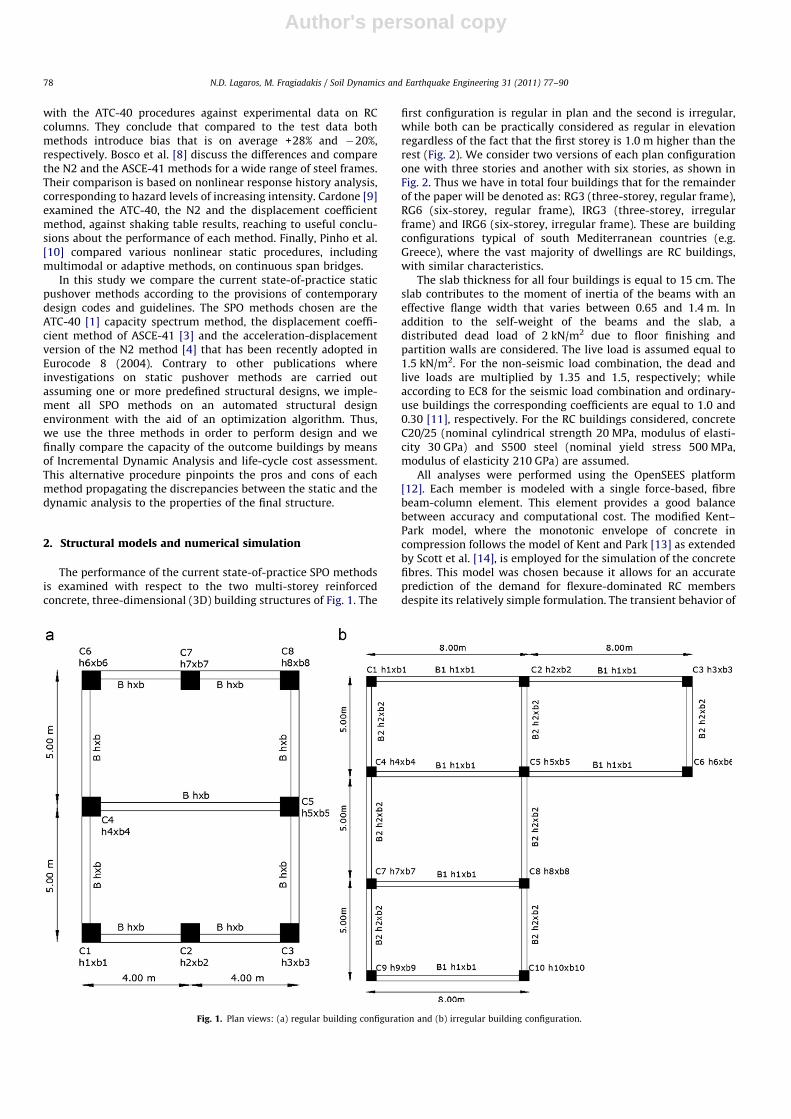
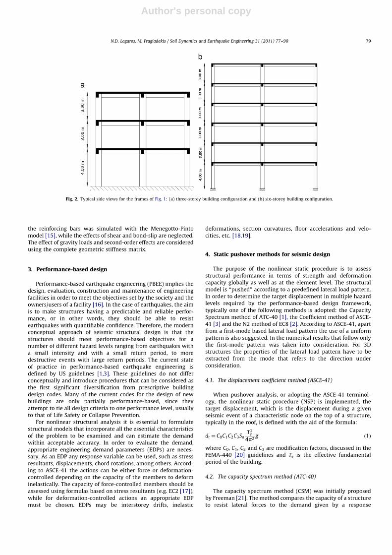
The performance of the current state-of-practice SPO methodsis examined with respect to the two multi-storey reinforcedconcrete, three-dimensional (3D) building structures of Fig. 1. The

first configuration is regular in plan and the second is irregular,while both can be practically considered as regular in elevationregardless of the fact that the first storey is 1.0 m higher than therest (Fig. 2). We consider two versions of each plan configurationone with three stories and another with six stories, as shown inFig. 2. Thus we have in total four buildings that for the remainderof the paper will be denoted as: RG3 (three-storey, regular frame),RG6 (six-storey, regular frame), IRG3 (three-storey, irregularframe) and IRG6 (six-storey, irregular frame). These are buildingconfigurations typical of south Mediterranean countries (e.g.Greece), where the vast majority of dwellings are RC buildings,with similar characteristics.

The slab thickness for all four buildings is equal to 15 cm. Theslab contributes to the moment of inertia of the beams with aneffective flange width that varies between 0.65 and 1.4 m. Inaddition to the self-weight of the beams and the slab, adistributed dead load of 2 kN/m2 due to floor finishing andpartition walls are considered. The live load is assumed equal to1.5 kN/m2. For the non-seismic load combination, the dead andlive loads are multiplied by 1.35 and 1.5, respectively; whileaccording to EC8 for the seismic load combination and ordinary-use buildings the corresponding coefficients are equal to 1.0 and0.30 [11], respectively. For the RC buildings considered, concreteC20/25 (nominal cylindrical strength 20 MPa, modulus of elasti-city 30 GPa) and S500 steel (nominal yield stress 500 MPa,modulus of elasticity 210 GPa) are assumed.

All analyses were performed using the OpenSEES platform[12]. Each member is modeled with a single force-based, fibrebeam-column element. This element provides a good balancebetween accuracy and computational cost. The modified Kent–Park model, where the monotonic envelope of concrete incompression follows the model of Kent and Park [13] as extendedby Scott et al. [14], is employed for the simulation of the concretefibres. This model was chosen because it allows for an accurateprediction of the demand for flexure-dominated RC membersdespite its relatively simple formulation. The transient behavior of

Fig. 1. Plan views: (a) regular building configuration and (b) irregular building configuration.

N.D. Lagaros, M. Fragiadakis / Soil Dynamics and Earthquake Engineering 31 (2011) 77–9078


the reinforcing bars was simulated with the Menegotto-Pintomodel [15], while the effects of shear and bond-slip are neglected.The effect of gravity loads and second-order effects are consideredusing the complete geometric stiffness matrix.

3. Performance-based design

Performance-based earthquake engineering (PBEE) implies thedesign, evaluation, construction and maintenance of engineeringfacilities in order to meet the objectives set by the society and theowners/users of a facility [16]. In the case of earthquakes, the aimis to make structures having a predictable and reliable perfor-mance, or in other words, they should be able to resistearthquakes with quantifiable confidence. Therefore, the modernconceptual approach of seismic structural design is that thestructures should meet performance-based objectives for anumber of different hazard levels ranging from earthquakes witha small intensity and with a small return period, to moredestructive events with large return periods. The current stateof practice in performance-based earthquake engineering isdefined by US guidelines [1,3]. These guidelines do not differconceptually and introduce procedures that can be considered asthe first significant diversification from prescriptive buildingdesign codes. Many of the current codes for the design of newbuildings are only partially performance-based, since theyattempt to tie all design criteria to one performance level, usuallyto that of Life Safety or Collapse Prevention.

For nonlinear structural analysis it is essential to formulatestructural models that incorporate all the essential characteristicsof the problem to be examined and can estimate the demandwithin acceptable accuracy. In order to evaluate the demand,appropriate engineering demand parameters (EDPs) are neces-sary. As an EDP any response variable can be used, such as stressresultants, displacements, chord rotations, among others. Accord-ing to ASCE-41 the actions can be either force or deformation-controlled depending on the capacity of the members to deforminelastically. The capacity of force-controlled members should beassessed using formulas based on stress resultants (e.g. EC2 [17]),while for deformation-controlled actions an appropriate EDPmust be chosen. EDPs may be interstorey drifts, inelastic

deformations, section curvatures, floor accelerations and velo-cities, etc. [18,19].

4. Static pushover methods for seismic design

The purpose of the nonlinear static procedure is to assessstructural performance in terms of strength and deformationcapacity globally as well as at the element level. The structuralmodel is ‘‘pushed’’ according to a predefined lateral load pattern.In order to determine the target displacement in multiple hazardlevels required by the performance-based design framework,typically one of the following methods is adopted: the CapacitySpectrum method of ATC-40 [1], the Coefficient method of ASCE-41 [3] and the N2 method of EC8 [2]. According to ASCE-41, apartfrom a first-mode based lateral load pattern the use of a uniformpattern is also suggested. In the numerical results that follow onlythe first-mode pattern was taken into consideration. For 3Dstructures the properties of the lateral load pattern have to beextracted from the mode that refers to the direction underconsideration.

4.1. The displacement coefficient method (ASCE-41)

When pushover analysis, or adopting the ASCE-41 terminol-ogy, the nonlinear static procedure (NSP) is implemented, thetarget displacement, which is the displacement during a givenseismic event of a characteristic node on the top of a structure,typically in the roof, is defined with the aid of the formula:

dt ¼ C0C1C2C3SaT2

e

4p2g ð1Þ

where C0, C1, C2 and C3 are modification factors, discussed in theFEMA-440 [20] guidelines and Te is the effective fundamentalperiod of the building.

4.2. The capacity spectrum method (ATC-40)

The capacity spectrum method (CSM) was initially proposedby Freeman [21]. The method compares the capacity of a structureto resist lateral forces to the demand given by a response

Fig. 2. Typical side views for the frames of Fig. 1: (a) three-storey building configuration and (b) six-storey building configuration.

N.D. Lagaros, M. Fragiadakis / Soil Dynamics and Earthquake Engineering 31 (2011) 77–90 79


spectrum. The response spectrum represents the demand whilethe pushover curve (or the ‘capacity curve’) represents theavailable capacity. Among the three variations of the methoddiscussed in ATC-40, we examine Procedure A. The steps of themethod are briefly summarized as follows: (i) Perform pushoveranalysis and determine the capacity curve in base shear (Vb)versus roof displacement of the building (D). This diagram is thenconverted to acceleration–displacement terms (AD) using anequivalent single degree of system (ESDOF). The conversion isperformed using the first mode participation factor C0 (D*

¼D/C0)and the modal mass (A¼Vb/M). (ii) Plot the capacity diagram onthe same graph with the 5%-damped elastic response spectrumthat is also in AD format. (iii) Select a trial peak deformationdemand d�t and determine the corresponding pseudo-accelerationA from the capacity diagram, initially assuming z¼5%. (iv)Compute ductility m¼D*/uy and calculate the hysteretic dampingzh as zh¼2(m�1)/pm. The equivalent damping ratio is evaluatedfrom a relationship of the form:zeq ¼ zelþkzh, where k is adamping modification factor that depends on the hystereticbehavior of the system. Update the estimate of d�t using the elasticdemand diagram for zeq. (v) Check for convergence the displace-ment d�t . When convergence has been achieved the targetdisplacement of the MDOF system is equal to dt ¼ C0d�t .

4.3. The N2 method (EC8)

The N2 method was initially proposed by Fajfar [22,23] andwas later expressed in a displacement-acceleration format [4].Recently, the method has been included in the Eurocode 8 (2004).Conceptually the method is a variation of Capacity SpectrumMethod that instead of highly damped spectra uses an R–m–T

relationship. The method, as implemented in EC8, consists of thefollowing steps: (i) Perform pushover analysis and obtain thecapacity curve in Vb–D terms, (ii) convert the pushover curve ofthe MDOF system to the capacity diagram of an ESDOF systemand approximate the capacity curve with an idealized elasto-perfectly plastic relationship to get the period Te of the ESDOF, (iii)the target displacement is then calculated as

d�et ¼ SaðTeÞTe

2p

� �2

ð2Þ

where Sa(Te) is the elastic acceleration response spectrum at theperiod Te. To determine the target displacement d�t , differentexpressions are suggested for the short and the medium to long-period ranges, thus:� T*oTC (short period range): If F�y=m�ZSaðTeÞ, the response is

elastic and thus d�t ¼ d�et and dt ¼ C0d�t . Otherwise the response isnonlinear and the ESDOF maximum displacement is calculated as

d�t ¼d�et

qu1þðqu�1Þ

TC

Te

� �Zd�et ð3Þ

where qu is the ratio of the acceleration of the structure withunlimited elastic capacity times the modal mass m* over its yieldforce, or simply: qu ¼ SaðTeÞm�=F�y .� T*ZTC (medium and long period range): The target

displacement of the inelastic system is equal to that of an elasticstructure, thus d�t ¼ d�et . The displacement of the MDOF system isalways calculated as dt ¼ C0d�t .

5. Preliminary evaluation of static pushover methods

Initially we examine the influence of different state-of-practiceSPO methods on the variation of two commonly adoptedengineering demand parameters (EDPs), the maximum interstor-ey drift (ymax) and the maximum roof drift (yroof). We perform a

preliminary analysis to compare the three methods on a given RCbuilding configuration, thus following the most common andconceptually straightforward approach to compare two analysismethods. The results of the SPO methods are compared to those ofthe Incremental Dynamic Analysis (IDA) method [24] for theregular in plan, three-storey structure (RG3).

For this comparison we adopt an arbitrary design of the RG3building configuration. Thus, the columns are considered to havedimensions 40�40 cm2 and 8Ø22 reinforcement, while thebeams are of 25�50 cm2 with 6Ø20 bars. In total the weight ofthe reinforcement steel is equal to 1910 and 1705 kg while theconcrete volume is equal to 12.8 and 14.4 m3 for the columns andbeams, respectively. The base shear was obtained from theresponse spectrum for soil type B (characteristic periods TB¼0.15s, TC¼0.50 s and TD¼2.00 s), while the PGA considered is equal to0.32 g. Moreover, the importance factor gI was taken equal to 1.0,while the damping correction factor is equal to 1.0, since adamping ratio of 5% has been considered.

IDA is here performed in the form of multi-stripe analysis,according to the notation of Jalayer [25]. To this cause a suite oftwenty strong ground motion records is adopted. The twentyrecords and their properties are listed in Table 1, where PGAlong

and PGAtran stands for the peek ground acceleration along thelongitudinal and transverse directions, respectively. The recordsare scaled to four levels of seismic intensity, represented by acommon intensity measure (IM). The chosen IM is the 5%-damped, first mode spectral acceleration, denoted as Sa(T1,5%).Therefore, all records are scaled to the same Sa(T1,5%) values,obtained from the EC8 elastic spectrum for peak groundacceleration (PGA) values equal to 0.16, 0.24, 0.30 and 0.50 g.Following the terminology of ASCE-41, the PGA values refer to thefollowing performance levels: operational (O), immediate occu-pancy (IO), life safety (LS) and collapse prevention (CP),respectively. In order to preserve the relative scale of the twocomponents of the records, the scaling factor of every record isobtained from the component with the larger PGA value and is thesame for both components of the record. When IDA is performed,we obtain 16%, 50% and 84% fractiles of the chosen EDP. The 50%fractile is the median demand, conditional on the intensitymeasure IM, while the 16%, 84% fractiles are used to provide ameasure of dispersion around the median.

The EDPs examined are the maximum interstorey drift, ymax,and the maximum roof drift in the two building directions, yX

roof

and yYroof . According to the recommendation of ASCE-41, the

multidirectional effect is accounted as the sum of the 100% of theresponse due to loading in the longitudinal direction and the 30%of the response in the transverse direction, and vice versa.Although this recommendation refers to forces, it was hereadopted to combine the drift ymax values. Thus, the ymax valuesshown are the maximum values of the SRSS combination of thecorresponding yX

max and yYmax values, along the height of the

building:

ymax ¼maxðffiffiffiffiffiffiffiffiffiffiffiffiffiffiffiffiffiffiffiffiffiffiffiffiffiffiffiffiffiffiffiffiffiffiffiffiffiffiffiffiffiffiðyX

maxÞ2þð0:3yY

maxÞ2

q,ffiffiffiffiffiffiffiffiffiffiffiffiffiffiffiffiffiffiffiffiffiffiffiffiffiffiffiffiffiffiffiffiffiffiffiffiffiffiffiffiffiffiðyY

maxÞ2þð0:3yX

maxÞ2

qÞ ð4Þ

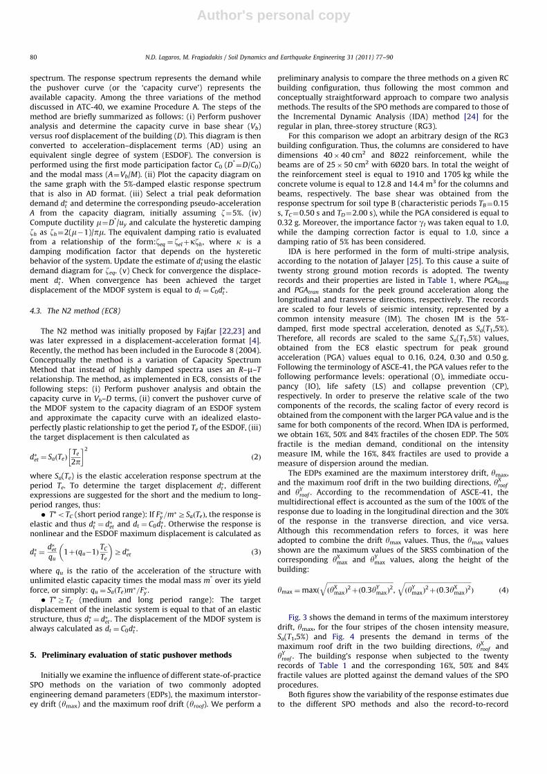
Fig. 3 shows the demand in terms of the maximum interstoreydrift, ymax, for the four stripes of the chosen intensity measure,Sa(T1,5%) and Fig. 4 presents the demand in terms of themaximum roof drift in the two building directions, yX

roof andyY

roof . The building’s response when subjected to the twentyrecords of Table 1 and the corresponding 16%, 50% and 84%fractile values are plotted against the demand values of the SPOprocedures.

Both figures show the variability of the response estimates dueto the different SPO methods and also the record-to-record



variability of IDA. In particular, for all four intensity levels the N2and the ASCE-41 results practically coincide with the median ymax

of the IDA method. On the other hand the capacity spectrummethod of ATC-40 produces slightly higher predictions for thefirst three Sa(T1,5%) intensities, while as the IM level increases, thedemand approaches the 16% fractile.

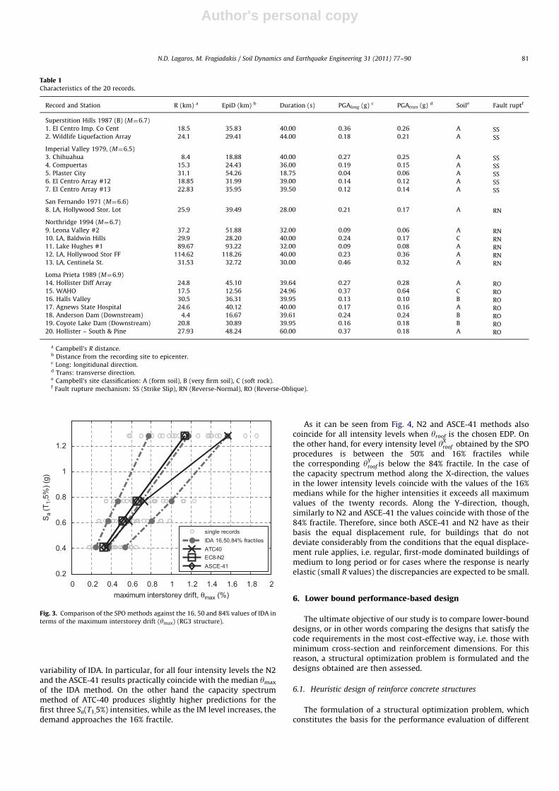
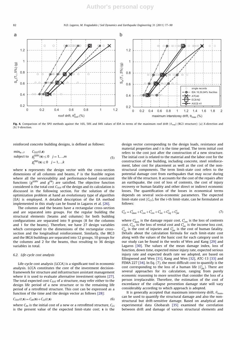
As it can be seen from Fig. 4, N2 and ASCE-41 methods alsocoincide for all intensity levels when yroof is the chosen EDP. Onthe other hand, for every intensity level yX

roof obtained by the SPOprocedures is between the 50% and 16% fractiles whilethe corresponding yY

roof is below the 84% fractile. In the case ofthe capacity spectrum method along the X-direction, the valuesin the lower intensity levels coincide with the values of the 16%medians while for the higher intensities it exceeds all maximumvalues of the twenty records. Along the Y-direction, though,similarly to N2 and ASCE-41 the values coincide with those of the84% fractile. Therefore, since both ASCE-41 and N2 have as theirbasis the equal displacement rule, for buildings that do notdeviate considerably from the conditions that the equal displace-ment rule applies, i.e. regular, first-mode dominated buildings ofmedium to long period or for cases where the response is nearlyelastic (small R values) the discrepancies are expected to be small.

6. Lower bound performance-based design

The ultimate objective of our study is to compare lower-bounddesigns, or in other words comparing the designs that satisfy thecode requirements in the most cost-effective way, i.e. those withminimum cross-section and reinforcement dimensions. For thisreason, a structural optimization problem is formulated and thedesigns obtained are then assessed.

6.1. Heuristic design of reinforce concrete structures

The formulation of a structural optimization problem, whichconstitutes the basis for the performance evaluation of different

Table 1Characteristics of the 20 records.

Record and Station R (km) a EpiD (km) b Duration (s) PGAlong (g) c PGAtran (g) d Soile Fault ruptf

Superstition Hills 1987 (B) (M¼6.7)

1. El Centro Imp. Co Cent 18.5 35.83 40.00 0.36 0.26 A SS2. Wildlife Liquefaction Array 24.1 29.41 44.00 0.18 0.21 A SS

Imperial Valley 1979, (M¼6.5)

3. Chihuahua 8.4 18.88 40.00 0.27 0.25 A SS4. Compuertas 15.3 24.43 36.00 0.19 0.15 A SS5. Plaster City 31.1 54.26 18.75 0.04 0.06 A SS6. El Centro Array #12 18.85 31.99 39.00 0.14 0.12 A SS7. El Centro Array #13 22.83 35.95 39.50 0.12 0.14 A SS

San Fernando 1971 (M¼6.6)

8. LA, Hollywood Stor. Lot 25.9 39.49 28.00 0.21 0.17 A RN

Northridge 1994 (M¼6.7)

9. Leona Valley #2 37.2 51.88 32.00 0.09 0.06 A RN10. LA, Baldwin Hills 29.9 28.20 40.00 0.24 0.17 C RN11. Lake Hughes #1 89.67 93.22 32.00 0.09 0.08 A RN12. LA, Hollywood Stor FF 114.62 118.26 40.00 0.23 0.36 A RN13. LA, Centinela St. 31.53 32.72 30.00 0.46 0.32 A RN

Loma Prieta 1989 (M¼6.9)

14. Hollister Diff Array 24.8 45.10 39.64 0.27 0.28 A RO15. WAHO 17.5 12.56 24.96 0.37 0.64 C RO16. Halls Valley 30.5 36.31 39.95 0.13 0.10 B RO17. Agnews State Hospital 24.6 40.12 40.00 0.17 0.16 A RO18. Anderson Dam (Downstream) 4.4 16.67 39.61 0.24 0.24 B RO19. Coyote Lake Dam (Downstream) 20.8 30.89 39.95 0.16 0.18 B RO20. Hollister – South & Pine 27.93 48.24 60.00 0.37 0.18 A RO

a Campbell’s R distance.b Distance from the recording site to epicenter.c Long: longitidunal direction.d Trans: transverse direction.e Campbell’s site classification: A (form soil), B (very firm soil), C (soft rock).f Fault rupture mechanism: SS (Strike Slip), RN (Reverse-Normal), RO (Reverse-Oblique).

0 0.2 0.4 0.6 0.8 1 1.2 1.4 1.6 1.8 20.2

0.4

0.6

0.8

1

1.2

maximum interstorey drift, θmax (%)

Sa

(T1,

5%) (

g)

single recordsIDA 16,50,84% fractilesATC40EC8-N2ASCE-41

Fig. 3. Comparison of the SPO methods against the 16, 50 and 84% values of IDA in

terms of the maximum interstorey drift (ymax) (RG3 structure).



reinforced concrete building designs, is defined as follows:

minsA F CTOT ðt,sÞ

subject to gSERVj ðsÞr0 j¼ 1,:::,m

gPBDj ðsÞr0 j¼ 1,:::,k

ð5Þ

where s represents the design vector with the cross-sectiondimensions of all columns and beams, F is the feasible regionwhere all the serviceability and performance-based constraintfunctions (gSERV and gPB) are satisfied. The objective functionconsidered is the total cost CTOT of the design and its calculation isdiscussed in the following section. For the solution of theoptimization problem at hand an evolutionary type of algorithm(EA) is employed. A detailed description of the EA methodimplemented in this study can be found in Lagaros et al. [26].

The columns and the beams have a rectangular cross-sectionand are separated into groups. For the regular building thestructural elements (beams and columns) for both buildingconfigurations are separated into 9 groups (8 for the columnsand 1 for the beams). Therefore, we have 27 design variableswhich correspond to the dimensions of the rectangular cross-section and the longitudinal reinforcement. Similarly, the IRG3and the IRG6 buildings are separated into 12 groups, 10 groups forthe columns and 2 for the beams, thus resulting to 36 designvariables in total.

6.2. Life-cycle cost analysis

Life-cycle cost analysis (LCCA) is a significant tool in economicanalysis. LCCA constitutes the core of the investment decision-framework for structure and infrastructure assistant managementwhere it is used to evaluate alternative investment options [27].The total expected cost CTOT of a structure, may refer either to thedesign life period of a new structure or to the remaining lifeperiod of a retrofitted structure. This cost can be expressed as afunction of the time and the design vector as follows [28]:

CTOT ðt,sÞ ¼ CINðsÞþCLSðt,sÞ ð6Þ

where CIN is the initial cost of a new or a retrofitted structure, CLS

is the present value of the expected limit-state cost; s is the

design vector corresponding to the design loads, resistance andmaterial properties and t is the time period. The term initial costrefers to the cost just after the construction of a new structure.The initial cost is related to the material and the labor cost for theconstruction of the building, including concrete, steel reinforce-ment, labor cost for placement as well as the cost of the non-structural components. The term limit-state cost refers to thepotential damage cost from earthquakes that may occur duringthe life of the structure. It accounts for the cost of the repairs afteran earthquake, the cost of loss of contents, the cost of injuryrecovery or human fatality and other direct or indirect economiclosses. The quantification of the losses in economical termsdepends on several socio-economic parameters. The expectedlimit-state cost (CLS), for the i-th limit-state, can be formulated asfollows:

CiLS ¼ Ci

damþCiconþCi

renþCiincþCi

injþCifat ð7Þ

where Cidam is the damage repair cost, Ci

con is the loss of contentscost, Ci

ren is the loss of rental cost and Ciinc is the income loss cost,

Ciinj is the cost of injuries and Ci

fat is the cost of human fatality.Details about the calculation formula for each limit-state costalong with the values of the basic cost for each category used inour study can be found in the works of Wen and Kang [29] andLagaros [30]. The values of the mean damage index, loss offunction, down time, expected minor injury rate, expected seriousinjury rate and expected death rate we adopted, are based onEllingwood and Wen [31], Kang and Wen [32], ATC-13 [33] andFEMA 227 [34]. In Eq. (7), the most difficult cost to quantify is thecost corresponding to the loss of a human life (Ci

fat). There areseveral approaches for its calculation, ranging from purelyeconomic reasoning to more sensitive that consider the loss of aperson irreplaceable. Therefore, the estimation of the cost ofexceedance of the collapse prevention damage state will varyconsiderably according to which approach is adopted.

It is generally accepted that maximum interstorey drift, ymax,can be used to quantify the structural damage and also the non-structural but drift-sensitive damage. Based on analytical andexperimental data Ghobarah [35] examined the correlationbetween drift and damage of various structural elements and

0 0.2 0.4 0.6 0.8 1 1.20.2

0.4

0.6

0.8

1

1.2

roof drift, θXroof (%)

Sa

(T1

,5%

) (g)

Sa

(T1

,5%

) (g)

0 0.2 0.4 0.6 0.8 1 1.2 1.4 1.6 1.8 20.2

0.4

0.6

0.8

1

1.2


single recordsIDA 16,50,84% fractilesATC40EC8-N2ASCE-41

Fig. 4. Comparison of the SPO methods against the 16%, 50% and 84% values of IDA in terms of the maximum roof drift (yroof) (RG3 structure): (a) X-direction and

(b) Y-direction.



systems. He determined the relationship between interstoreydrift and various damage levels of different reinforced concreteelements and structural systems.

Based on the Poisson model of earthquake occurrence andthe assumption that after a major damage-inducing seismic event,the building is immediately retrofitted to its original intactconditions, Wen and Kang [28,29] proposed the following formulafor the expected life-cycle cost considering N damage states:

CLSðt,sÞ ¼nlð1�e�ltÞ

XN

i ¼ 1

CiLSPi ð8Þ

Pðymax4yimaxÞ ¼ ð�1=tÞln½1�Pðymax4yi

maxÞ�

Pi ¼ Pðymax4yimaxÞ�Pðymax4yiþ1

maxÞ ð9Þ

According to Eq. (8) the limit-state costs CiLSof Eq. (8) are used

to calculateCLSðt,sÞ, where Pi is the probability of the ith damagestate being violated given the occurrence of an earthquake. Eq. (9)assumes the maximum interstorey drift ymax as the characteristicEDP, while P(ymax4yi

max) is the exceedance probability givenoccurrence. ymax and yi

max are the drift ratios that define the lowerand upper bounds of the ith damage state and Pi(ymax�y

imax) is

the annual exceedance probability of the maximum interstoreydrift value yi

max. Finally, n is the annual occurrence rate ofsignificant earthquakes modeled as a Poisson variable. Theexponential component of Eq. (8) is used to express CLS in presentvalue, where l is the annual momentary discount rate. The annualmomentary discount rate is typically taken to be constant andequal to 5% [36], while its value lies in the range of 3–6%. Eachdamage state is defined by appropriate drift ratio limits depend-ing on the type of structure, e.g. steel or RC structure (Table 2).When one of the limit-state drifts is reached, the correspondinglimit-state is assumed to be exceeded. Parameters a1 and a2 areobtained by best fit of known pairs Pi�y

imax and the annual

exceedance probability Pi is obtained from a relationship of the

form (Table 3):

Piðymax�yimaxÞ ¼ a1ðy

imaxÞ

�a2 ð10Þ

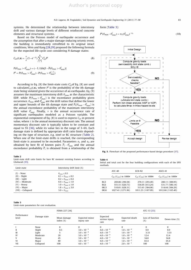
Table 2Limit-state drift ratio limits for bare RC moment resisting frames according to

Ghobarah [35].

Limit-state Interstorey drift limit (%)

(I) – None ymaxr0.1

(II) – Slight 0.1oymaxr0.2

(III) – Light 0.2oymaxr0.4

(IV) – Moderate 0.4oymaxr1.0

(V) – Heavy 1.0oymaxr1.8

(VI) – Major 1.8oymaxr3.0

(VII) – Collapsed 3.0oymax

Table 3Limit-state parameters for cost evaluation.

Performance

levelDamage state

FEMA-227 [34] ATC-13 [33]

Mean damage

index (%)

Expected minor

injury rate

Expected

serious injury

rate

Expected death

rate

Loss of function

(%)Down time (%)

I None 0 0 0 0 0 0

II Slight 0.5 3.0�10�5 4.0�10�6 1.0�10�6 0.9 0.9

III Light 5 3.0�10�4 4.0�10�5 1.0�10�5 3.33 3.33

IV Moderate 20 3.0�10�3 4.0�10�4 1.0�10�4 12.4 12.4

V Heavy 45 3.0�10�2 4.0�10�3 1.0�10�3 34.8 34.8

VI Major 80 3.0�10�1 4.0�10�2 1.0�10�2 65.4 65.4

VII Collapsed 100 4.0�10�1 4.0�10�1 2.0�10�1 100 100

Fig. 5. Flowchart of the proposed performance-based design procedure [37].

Table 4Initial and total cost for the four building configurations with each of the SPO

methods.

ATC-40 EC8-N2 ASCE-41

CIN (CTOT) in 1000h CIN (CTOT) in 1000h CIN (CTOT) in 1000h

RG3 269.86 (296.58) 270.11 (293.49) 280.11 (300.95)

RG6 551.51 (620.73) 536.05 (613.24) 531.77 (586.14)

IRG3 510.81 (628.31) 513.41 (584.06) 514.64 (584.29)

IRG6 1027.41 (1271.96) 1011.23 (1187.09) 1012.66 (1165.49)



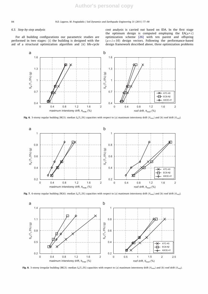
6.3. Step-by-step analysis

For all building configurations our parametric studies areperformed in two stages: (i) the building is designed with theaid of a structural optimization algorithm and (ii) life-cycle

cost analysis is carried out based on IDA. In the first stagethe optimum design is computed employing the EA(m+l)optimization scheme [26] with ten parent and offspring(m¼l¼10) design vectors. Following the performance-baseddesign framework described above, three optimization problems

0 0.4 0.8 1.2 1.6 20.4

0.7

1

1.3

1.6


Sa

(T1,

5%) (

g)

Sa

(T1,

5%) (

g)0 0.4 0.8 1.2 1.6 2

0.4

0.7

1

1.3

1.6

roof drift, θroof (%)

ATC-40EC8-N2ASCE-41

Fig. 6. 3-storey regular building (RG3): median Sa(T1,5%) capacities with respect to (a) maximum interstorey drift (ymax) and (b) roof drift (yroof).

0 0.4 0.8 1.2 1.6 20.2

0.4

0.6

0.8

1


Sa

(T1,

5%) (

g)

Sa

(T1,

5%) (

g)

0 0.4 0.8 1.2 1.6 20.2

0.4

0.6

0.8

1


ATC-40EC8-N2ASCE-41

Fig. 7. 6-storey regular building (RG6): median Sa(T1,5%) capacities with respect to (a) maximum interstorey drift (ymax) and (b) roof drift (yroof).

0 0.4 0.8 1.2 1.6 20.2

0.5

0.8

1.1

1.4


Sa

(T1,

5%) (

g)

Sa

(T1,

5%) (

g)

0 0.5 1 1.5 2 2.50.2

0.4

0.6

0.8

1


ATC-40EC8-N2ASCE-41

Fig. 8. 3-storey irregular building (IRG3): median Sa(T1,5%) capacities with respect to (a) maximum interstorey drift (ymax) and (b) roof drift (yroof).



are defined. The detailed description of the exact steps followedfor the seismic design of the buildings can be found in Lagarosand Papadrakakis [37], while a flowchart of this algorithmis presented in Fig. 5. According to Fig. 5 the static pushovermethods are nested in the iterative optimum design algorithm.

Moreover, for all four building configurations we calculate thetotal life-cycle cost which is the objective function to beminimized. In the second stage, life-cycle cost analysis isperformed on the optimum designs using IDA as the method toassess the capacity.

0 0.5 1 1.5 2 2.50.2

0.4

0.6

0.8

1


Sa

(T1,

5%) (

g)

Sa

(T1,

5%) (

g)0 0.5 1 1.5 2 2.5

0.2

0.4

0.6

0.8

1


ATC-40EC8-N2ASCE-41

Fig. 9. 6-storey irregular building (IRG6): median Sa(T1,5%) capacities with respect to (a) maximum interstorey drift (ymax) and (b) roof drift (yroof).

269.86 270.11

280.10

296.29

293.28

300.76296.58293.49

300.95

265

270

275

280

285

290

295

300

305

ATC40 EC8-N2 ASCE 41

Cos

t (10

00 €

)

Designs

CIN

TOT (I)

TOT (II)

Fig. 10. 3-storey regular building (RG3): (a) initial (CIN) and total expected (CTOT) life-cycle costs for the three SPO-based designs and (b) contribution of the initial cost and

limit-state cost components to the total expected life-cycle cost.



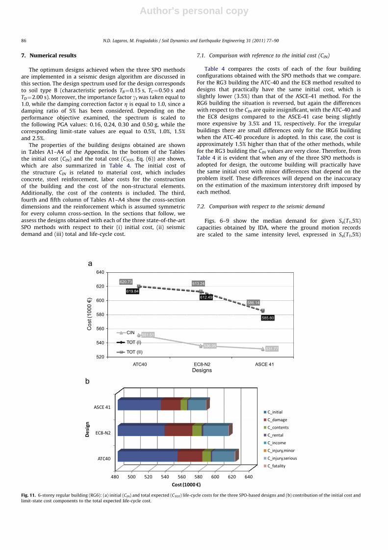
7. Numerical results

The optimum designs achieved when the three SPO methodsare implemented in a seismic design algorithm are discussed inthis section. The design spectrum used for the design correspondsto soil type B (characteristic periods TB¼0.15 s, TC¼0.50 s andTD¼2.00 s). Moreover, the importance factor gI was taken equal to1.0, while the damping correction factor Z is equal to 1.0, since adamping ratio of 5% has been considered. Depending on theperformance objective examined, the spectrum is scaled tothe following PGA values: 0.16, 0.24, 0.30 and 0.50 g, while thecorresponding limit-state values are equal to 0.5%, 1.0%, 1.5%and 2.5%.

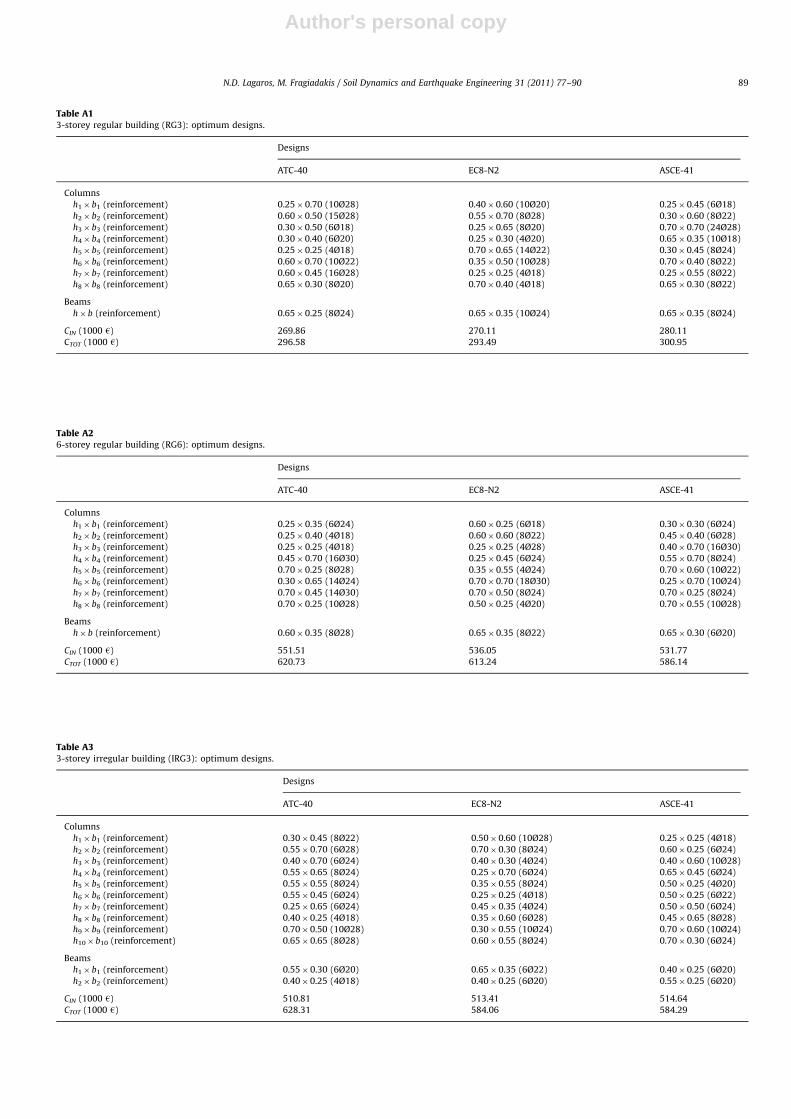
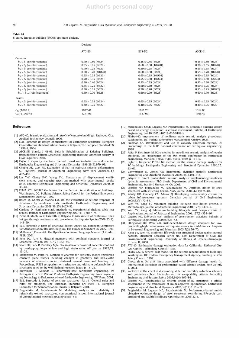
The properties of the building designs obtained are shownin Tables A1–A4 of the Appendix. In the bottom of the Tablesthe initial cost (CIN) and the total cost (CTOT, Eq. (6)) are shown,which are also summarized in Table 4. The initial cost ofthe structure CIN is related to material cost, which includesconcrete, steel reinforcement, labor costs for the constructionof the building and the cost of the non-structural elements.Additionally, the cost of the contents is included. The third,fourth and fifth column of Tables A1–A4 show the cross-sectiondimensions and the reinforcement which is assumed symmetricfor every column cross-section. In the sections that follow, weassess the designs obtained with each of the three state-of-the-artSPO methods with respect to their (i) initial cost, (ii) seismicdemand and (iii) total and life-cycle cost.

7.1. Comparison with reference to the initial cost (CIN)

Table 4 compares the costs of each of the four buildingconfigurations obtained with the SPO methods that we compare.For the RG3 building the ATC-40 and the EC8 method resulted todesigns that practically have the same initial cost, which isslightly lower (3.5%) than that of the ASCE-41 method. For theRG6 building the situation is reversed, but again the differenceswith respect to the CIN are quite insignificant, with the ATC-40 andthe EC8 designs compared to the ASCE-41 case being slightlymore expensive by 3.5% and 1%, respectively. For the irregularbuildings there are small differences only for the IRG6 buildingwhen the ATC-40 procedure is adopted. In this case, the cost isapproximately 1.5% higher than that of the other methods, whilefor the RG3 building the CIN values are very close. Therefore, fromTable 4 it is evident that when any of the three SPO methods isadopted for design, the outcome building will practically havethe same initial cost with minor differences that depend on theproblem itself. These differences will depend on the inaccuracyon the estimation of the maximum interstorey drift imposed byeach method.

7.2. Comparison with respect to the seismic demand

Figs. 6–9 show the median demand for given Sa(T1,5%)capacities obtained by IDA, where the ground motion recordsare scaled to the same intensity level, expressed in Sa(T1,5%)

551.51

536.05531.77

619.84612.49

585.60

620.73 613.24

586.14

520

540

560

580

600

620

640


Cos

t (10

00 €

)

Designs

CIN

TOT (I)

TOT (II)

Fig. 11. 6-storey regular building (RG6): (a) initial (CIN) and total expected (CTOT) life-cycle costs for the three SPO-based designs and (b) contribution of the initial cost and

limit-state cost components to the total expected life-cycle cost.



terms. The EDPs considered are the maximum interstorey drift(ymax) and the roof drift (yroof), both calculated according toEq. (4). The results shown have been obtained with the twentyrecords of Table 1, while for every intensity level we show onlythe median values obtained for each building design. For the RG3structure the ATC-40 procedure produces larger median demandscompared to the other two methods, regardless of the EDP (Fig. 6).The EC8 and the ASCE-41 approaches practically coincide whenymax is the EDP but some small differences are observed if thecomparison is performed with respect to yroof. Similarly for theRG6 building, the ATC-40 procedure causes larger demands(Fig. 7), while the difference on the median demands is significantfor both ymax and yroof comparisons. Especially for the yroof case(Fig. 7b) the EC8 produces slightly larger demands compared tothe ASCE-41 approach.

For the six-storey buildings (RG6, IRG6) the ASCE-41 approachproduces the smallest drift demands as was also the case with theRG3 structure, while the larger demands are those of the ATC-40method. The EC8 approach fans between the demands of the othertwo SPO methods and is closer to the ATC-40 prediction for theregular case and to ASCE-41 for the irregular building. In general,from Figs. 6–9, it is seen that the ATC-40 method produces buildingsmore flexible and therefore with larger demands, compared to theother methods, while and the opposite applies for the ASCE-41method. This behavior, to some extent, explains the findings of thecomparison with respect to the initial cost. The design with largestCIN is expected to have the smallest drift demand.

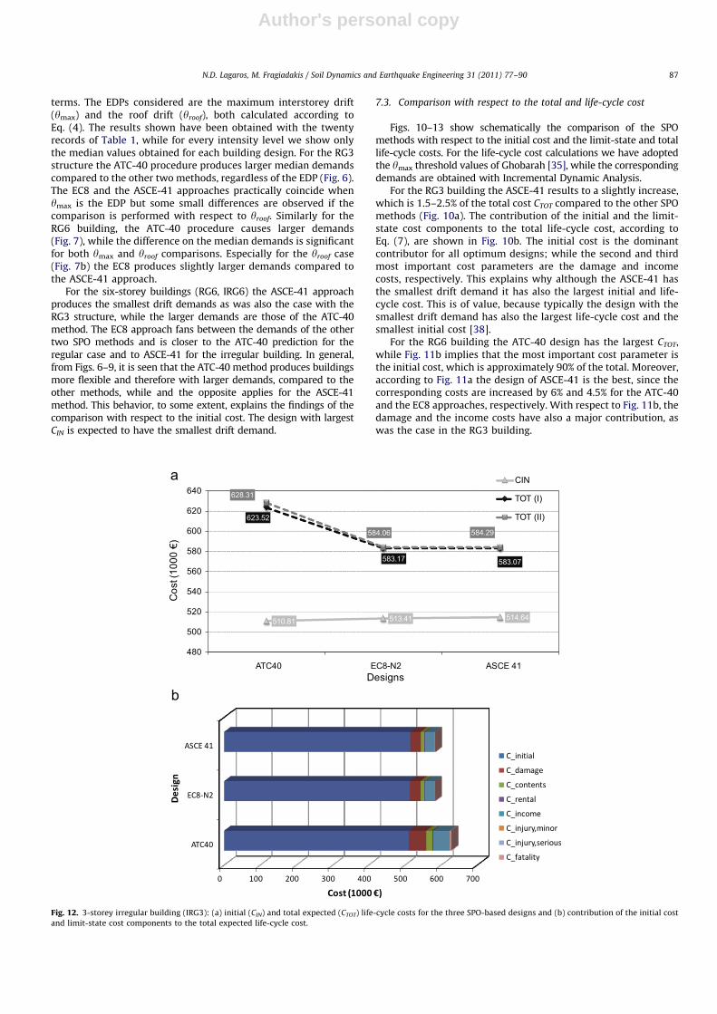
7.3. Comparison with respect to the total and life-cycle cost

Figs. 10–13 show schematically the comparison of the SPOmethods with respect to the initial cost and the limit-state and totallife-cycle costs. For the life-cycle cost calculations we have adoptedthe ymax threshold values of Ghobarah [35], while the correspondingdemands are obtained with Incremental Dynamic Analysis.

For the RG3 building the ASCE-41 results to a slightly increase,which is 1.5–2.5% of the total cost CTOT compared to the other SPOmethods (Fig. 10a). The contribution of the initial and the limit-state cost components to the total life-cycle cost, according toEq. (7), are shown in Fig. 10b. The initial cost is the dominantcontributor for all optimum designs; while the second and thirdmost important cost parameters are the damage and incomecosts, respectively. This explains why although the ASCE-41 hasthe smallest drift demand it has also the largest initial and life-cycle cost. This is of value, because typically the design with thesmallest drift demand has also the largest life-cycle cost and thesmallest initial cost [38].

For the RG6 building the ATC-40 design has the largest CTOT,while Fig. 11b implies that the most important cost parameter isthe initial cost, which is approximately 90% of the total. Moreover,according to Fig. 11a the design of ASCE-41 is the best, since thecorresponding costs are increased by 6% and 4.5% for the ATC-40and the EC8 approaches, respectively. With respect to Fig. 11b, thedamage and the income costs have also a major contribution, aswas the case in the RG3 building.

510.81 513.41 514.64

623.52

583.17 583.07

628.31

584.06 584.29

480

500

520

540

560

580

600

620

640


Cos

t (10

00 €

)

Designs

CIN

TOT (I)

TOT (II)

Fig. 12. 3-storey irregular building (IRG3): (a) initial (CIN) and total expected (CTOT) life-cycle costs for the three SPO-based designs and (b) contribution of the initial cost

and limit-state cost components to the total expected life-cycle cost.



Figs. 12 and 13 show the performance of the three designmethods for the irregular buildings (IRG3, IRG6). For both buildingconfigurations and regardless of the SPO method, initial cost isdominant in the calculation of the total life-cycle cost (Figs. 12and 13b). Furthermore, although the initial cost is practically thesame regardless of the SPO method the ATC-40 design has largertotal cost for 7.5% for the three-storey building and 9% for the six-storey one, while the differences between the other two methodsare very small.

8. Conclusions

In this study we performed an investigation on the influence ofalternative static pushover methods when adopted for the seismicdesign of new structures. The numerical investigation wasperformed on four multi-storey reinforced concrete buildings,with symmetrical and non-symmetrical plans, that have beenoptimally designed. The current trend in evaluating investmentpractices in structures is to take into consideration the total life-cycle cost rather than the initial construction cost. In the presentstudy life-cycle cost analysis is employed for the assessment ofthe seismic performance of buildings designed using either thecapacity spectrum method of ATC-40, the N2 method of EC8 orthe displacement coefficient method of ASCE-41.

Based on the limited number of buildings examined, we wereable to compare the three SPO methods with respect to theproperties of the outcome designs for RC buildings. Although thefocus of the study is not to determine which of the three methods

is more accurate, our results indicate that the ATC-40 methodtends to overestimate the demand, while the differences betweenthe EC8 and the ASCE-41 methods are rather small for low andmedium levels of seismic intensity. More specifically the mainfindings of this study are summarized as follows:

1. The initial cost of reinforced concrete structures designedbased on ATC-40 varies compared to the designs obtainedaccording to N2 and ASCE-41 up to 3.7%, while similarvariability is encountered between the designs of N2 andASCE-41. On the other hand comparing the total life-cycle cost,the designs of ATC-40 varies in the range of 1.0–9.0% comparedto the design of N2 and ASCE-41. The corresponding variabilitybetween the designs of N2 and ASCE-41 is up to 4.5%.

2. Comparing, the contributing parts of the total life-cycle cost(Figs. 10–13), it is concluded that the initial cost, in all testexamples, is the first dominant contributor for all designs. Thesecond and the third most important cost parameters are thedamage and income costs, respectively. It is also worth mention-ing that, although the four designs differ significantly, injury andfatality costs represent only a small percentage of the total cost.

3. Depending on the design method employed increasingconstruction cost does not always mean that seismic safetyis also increases.

Appendix A

See Tables A1–A4.

,,

,

,

,

,

,

,

,,

,

,

,,

,

,

Fig. 13. 6-storey irregular building (IRG6): (a) initial (CIN) and total expected (CTOT) life-cycle costs for the three SPO-based designs and (b) contribution of the initial cost

and limit-state cost components to the total expected life-cycle cost.



Table A26-storey regular building (RG6): optimum designs.

Designs


Columns

h1� b1 (reinforcement) 0.25�0.35 (6Ø24) 0.60�0.25 (6Ø18) 0.30�0.30 (6Ø24)








Beams

h� b (reinforcement) 0.60�0.35 (8Ø28) 0.65�0.35 (8Ø22) 0.65�0.30 (6Ø20)

CIN (1000 h) 551.51 536.05 531.77

CTOT (1000 h) 620.73 613.24 586.14

Table A33-storey irregular building (IRG3): optimum designs.

Designs


Columns











Beams



CIN (1000 h) 510.81 513.41 514.64

CTOT (1000 h) 628.31 584.06 584.29

Table A13-storey regular building (RG3): optimum designs.

Designs


Columns









Beams

h�b (reinforcement) 0.65�0.25 (8Ø24) 0.65�0.35 (10Ø24) 0.65�0.35 (8Ø24)

CIN (1000 h) 269.86 270.11 280.11

CTOT (1000 h) 296.58 293.49 300.95



References

[1] ATC-40. Seismic evaluation and retrofit of concrete buildings. Redwood City:Applied Technology Council; 1996.

[2] EC8. Eurocode 8: Design of structures for earthquake resistance. EuropeanCommittee for Standardisation: Brussels, Belgium, The European Standard EN1998-1, 2004.

[3] ASCE/SEI Standard 41-06. Seismic Rehabilitation of Existing Buildings.prepublication edition. Structural Engineering Institute, American Society ofCivil Engineers; 2006.

[4] Fajfar P. Capacity spectrum method based on inelastic demand spectra.Earthquake Engineering and Structural Dynamics 1999;28(9):979–99.

[5] Chopra AK, Goel RK. Evaluation of NSP to estimate seismic deformation:SDF systems. Journal of Structural Engineering New York 2000;126(4):482–490.

[6] Lin Y-Y, Chang K-C, Wang Y-L. Comparison of displacement coeffi-cient method and capacity spectrum method with experimental resultsof RC columns. Earthquake Engineering and Structural Dynamics 2004;33:35–48.

[7] FEMA 273. NEHRP Guidelines for the Seismic Rehabilitation of Buildings.Washington, DC: Building Seismic Safety Council for the Federal EmergencyManagement Agency; 1997.

[8] Bosco M, Ghersi A, Marino EM. On the evaluation of seismic response ofstructures by nonlinear static methods. Earthquake Engineering andStructural Dynamics 2009;38(13):1465–82.

[9] Cardone D. Nonlinear static methods vs. experimental shaking table testresults. Journal of Earthquake Engineering 2007;11(6):847–75.

[10] Pinho R, Monteiro R, Casarotti C, Delgado R. Assessment of continuous spanbridges through nonlinear static procedures. Earthquake Spectra 2009;25(1):143–59.

[11] EC0. Eurocode 0. Basis of structural design: Annex A1. European Committeefor Standardisation: Brussels, Belgium. The European Standard EN 2005. 1990.

[12] McKenna F, Fenves GL. The OpenSees Command Language Manual. (1.2. edn).PEER; 2001.

[13] Kent DC, Park R. Flexural members with confined concrete. Journal ofStructural Division 1971;97(7):1969–90.

[14] Scott BD, Park R, Priestley MJN. Stress–strain behavior of concrete confinedby overlapping hoops at low and high strain rates. ACI Journal 1982;79:13–27.

[15] Menegotto M, Pinto PE. Method of analysis for cyclically loaded reinforcedconcrete plane frames including changes in geometry and non-elasticbehavior of elements under combined normal force and bending. In:Proceedings, IABSE symposium on resistance and ultimate deformability ofstructures acted on by well defined repeated loads, p. 15–22.

[16] Krawinkler H, Miranda E. Performance-base earthquake engineering. In:Bozorgnia Y, Bertero Vitelmo V, editors. Earthquake Engineering: From Engineer-ing Seismology to Performance-based Earthquake Engineering. CRC Press; 2004.

[17] EC2. Eurocode 2. Design of concrete structures—Part 1: General rules andrules for buildings. The European Standard EN 1992-1-1. EuropeanCommittee for Standardisation: Brussels, Belgium; 2004.

[18] Fragiadakis M, Papadrakakis M. Modeling, analysis and reliability ofseismically excited structures: computational issues. International Journalof Computational Methods 2008;5(4):483–511.

[19] Mitropoulou ChCh, Lagaros ND, Papadrakakis M. Economic building designbased on energy dissipation: a critical assessment. Bulletin of EarthquakeEngineering, doi:10.1007/s10518-010-9182-x.

[20] FEMA-440. Improvement of nonlinear static seismic analysis procedures.Washington, DC: Federal Emergency Management Agency; 2005.

[21] Freeman SA. Development and use of capacity spectrum method. In:Proceedings of the 6 US national conference on earthquake engineering,1998.

[22] Fajfar P, Fischinger M. N2-a method for non-linear seismic analysis of regularbuildings. In: Proceedings of the 9th world conference on earthquakeengineering, Maruzen, Tokyo, 1988, Kyoto, 1989. p. 111–6.

[23] Fajfar P, Gaspersic P. The N2 method for the seismic damage analysis forRC buildings. Earthquake Engineering and Structural Dynamics 1996;25:23–67.

[24] Vamvatsikos D, Cornell CA. Incremental dynamic analysis. EarthquakeEngineering and Structural Dynamics 2002;31(3):491–514.

[25] Jalayer F. Direct probabilistic seismic analysis: implementing nonlineardynamic assessments. PhD thesis. Department of Civil and EnvironmentalEngineering, Stanford University, CA, 2003.

[26] Lagaros ND, Fragiadakis M, Papadrakakis M. Optimum design of shellstructures with stiffening beams. AIAA Journal 2004;42(1):175–84.

[27] Sahely HR, Kennedy CA, Adams BJ. Developing sustainability criteria forurban infrastructure systems. Canadian Journal of Civil Engineering2005;32(1):72–85.

[28] Wen YK, Kang YJ. Minimum building life-cycle cost design criteria. I:Methodology. Journal of Structural Engineering 2001;127(3):330–7.

[29] Wen YK, Kang YJ. Minimum building life-cycle cost design criteria. II:Applications. Journal of Structural Engineering 2001;127(3):338–46.

[30] Lagaros ND. Life-cycle cost analysis of construction practices. Bulletin ofEarthquake Engineering 2007;5:425–42.

[31] Ellingwood BR, Wen Y-K. Risk-benefit-based design decisions for low-probability/high consequence earthquake events in mid-America. Progressin Structural Engineering and Materials 2005;7(2):56–70.

[32] Kang Y-J, Wen YK. Minimum life-cycle cost structural design against naturalhazards, Structural Research Series No. 629. Department of Civil andEnvironmental Engineering, University of Illinois at Urbana-Champaign,Urbana, IL, 2000.

[33] ATC-13. Earthquake damage evaluation data for California. Redwood City,CA: Applied Technology Council; 1985.

[34] FEMA 227. A benefit–cost model for the seismic rehabilitation of buildings.Washington, DC: Federal Emergency Management Agency, Building SeismicSafety Council; 1992.

[35] Ghobarah A. On drift limits associated with different damage levels. In:International workshop on performance-based seismic design, June 28–July1, 2004.

[36] Rackwitz R. The effect of discounting, different mortality reduction schemesand predictive cohort life tables on risk acceptability criteria. ReliabilityEngineering and System Safety 2006;91(4):469–84.

[37] Lagaros ND, Papadrakakis M. Seismic design of RC structures: a criticalassessment in the framework of multi-objective optimization. EarthquakeEngineering and Structural Dynamics 2007;36(12):1623–39.

[38] Fragiadakis M, Lagaros ND, Papadrakakis M. Performance-based multi-objective optimum design of steel structures considering life-cycle cost.Structural and Multidisciplinary Optimization 2006;32:1.

Table A46-storey irregular building (IRG6): optimum designs.

Designs


Columns











Beams



CIN (1000 h) 1027.41 1011.23 1012.66

CTOT (1000 h) 1271.96 1187.09 1165.49


Evaluation of ASCE41, ATC40 and N2 static pushover methods based on optimally designed buildings

Documents

Transcript of Evaluation of ASCE41, ATC40 and N2 static pushover methods based on optimally designed buildings