The Resonant Retina: Exploiting VibrationNoise to Optimally Detect Edges in an ImageMax-Olivier Hongler, Yuri L. de Meneses, Member, IEEE, Antoine Beyeler, and Jacques Jacot

Abstract—We show that, far from being a drawback, the ubiquitous presence of random vibrations in vision systems operating from

mobile devices can advantageously be used as a fundamental tool for edge detection. Directly inspired by biology, the concept of

dynamic retina uses the random spatiotemporal path, traced by a moving receptor that samples the image over time, as the basis for

the edge detection operation. We propose a simple mathematical formalization of the dynamic retina concept that shows that the

relevant information needed for edge detection is contained in the modulation of the variance of the output signal delivered by the

retina. Based on a sequence of observations, we then use a variance estimator to determine the presence of the image edges.

Following again a biological inspiration, more specifically focusing on neuron dynamics, we introduce a threshold type estimator and

use its local asymptotic normality to optimize, via the Cramer-Rao relation, the value of the threshold. The optimal threshold value

coincides with a maximum of the associated Fisher information and the overall process can therefore be directly interpreted as a

stochastic resonance. We end our contribution by reporting some simple experimental illustrations.

Index Terms—Edge detection, random vibration of the optical axis, microsaccades, threshold variance estimator, Fisher information,

Cramer-Rao inequality, stochastic resonance.

�

1 INTRODUCTION

1.1 Motivation

MANY vision systems set on a mobile platform, such asaerial and satellite cameras, mobile-robotics vision

systems, and of course biological vision systems, have todeal with noise in the form of random vibrations aroundtheir optical axis. This vibration noise is traditionally seenas a nuisance. This paper intends to show that quite to thecontrary, this noise can be potentially exploited to extractinformation that is pertinent enough for edge detection.

Let us consider an individual sensing element, a pixel, ofsuch a vision system, and analyze its output signal along thetemporal axis when the sensor is subject to small amplitudevibrations. If the system is viewing a featureless, uniformly litscene such as in a foggy day, the output is not expected tochangemuch.On the contrary, if the pixel is “seeing” a regionof thescenewhere there isa transitionfromadark to lightarea,such as on the boundary of a dark object against lightbackground, the output signal will constantly vary from lowto high levels. Intuitively, higher contrast areas produce anoutput with higher variability and the output temporalaverage is related to the local average intensity. Since highcontrast regions are often associated with object boundaries,this approach provides quite useful information. This ob-servationwas firstmade by Prokopowicz andCooper [1] andthe present contribution mathematically formalizes theirbasic idea and proposes a way to extract the contrastinformation.

1.2 State-of-the-Art

Ever since vision systems have been mounted on mobileplatforms such as planes, satellites [2], cars or, more recently,mobile robots, engineers have had to tackle the problem ofnoise in the formof a random jittering of the optical axis.Untilthe 1990s, the computer vision community considered thesevibrationsof theopticalaxisasamerenuisanceanddevelopeda wealth of mechanical stabilization systems [2] and filteringtechniques [3] to eliminate this ubiquitous jittering.

In parallel to this classical engineering approach, lifescientists devoted a strong research activity to the study ofbiological vision systems.Oneof the interesting contributionsof these studies was the observation of the presence of small-amplitude movements in the human eye. These excitationsare now well-known under the name of microsaccades [4],[5]. Today, theultimate conclusions concerning theorigin, theexact nature, and the precise use of these microsaccades arestill lacking. Nevertheless, it is clearly established thatwithout these microscopic movements the photoreceptors“saturate” and the retinal images disappear.

Fully aware of this phenomenon, Prokopowicz andCooper [1] proposed a new vision device, called theDynamicRetina (DR), that directly takes advantage of the vibratingperturbations generated by mobile robots or any similar, mobileplatforms. The basic idea behind this pioneering work lies inthe fact that the spatiotemporal path, traced by a movingphotoreceptor that samples over time, canbeusedas thebasisfor neighborhood style image computations, i.e., purelyspatial computations. The authors [1] propose a phenomen-ological description of theirDRdevice andpresent the resultsof tests which were performed on an image sequence. Thereis, however, no formalizationordetailed statistical analysis ofthe system that would allow its tuning to particularsituations. Such a more formal description is one of the aimsof the present paper.

TheDRconceptoffersseveraladvantagesamongothers, itsmassive parallelism and the simplicity of its architecture.

IEEE TRANSACTIONS ON PATTERN ANALYSIS AND MACHINE INTELLIGENCE, VOL. 25, NO. 9, SEPTEMBER 2003 1051

. The authors are with the LPM/IPR/STI/IPR, �EEcole Polytechnique Federalede Lausanne, CH-1015 Lausanne, Switzerland.E-mail: {max-olivier.hongler, antoine.beyeler, jacques.jacot}@epfl.ch,yuri@ieee.org.

Manuscript received 22 May 2002; revised 28 Nov. 2002; accepted 4 Jan.2003.Recommended for acceptance by H. Christensen.For information on obtaining reprints of this article, please send e-mail to:tpami@computer.org, and reference IEEECS Log Number 116606.

0162-8828/03/$17.00 � 2003 IEEE Published by the IEEE Computer Society

Besides applications in the field of mobile robotics [6], thepotential interest of the DR concept has been recently furtherconfirmedby several newcontributions devoted to biologicalvisual systems. In particular, the studies devoted to the fly [7]and the jumping spider have established the presence of ascanning movement in their compound eyes. These resultshave further stimulated the conception of several artificialretinas operating in presence of vibrations, [8], [9], [10]. Thesepapers emphasize the resolution-enhancement property thatcan be achieved by such a scanning movement. This can beachieved if the actual displacement is deterministicallyknown. Inparticular,periodicmotionswerediscussed in [10].

In this paper, we offer a generalization that enables toexploit random mechanical excitations of the vision devices.We propose a simple mathematical modeling of theDR device in presence of a noise characterized by itsrelevant statistical properties. We focus our attention on theedge detection (ED) problem that is of fundamentalimportance for many vision systems. Indeed, as EDprovides a reduction in the amount of visual data, it is thefirst processing stage common to numerous vision systemsranging from computer vision [11], [12], [13] to biology [14],[15]. Edge detection is particularly difficult in the presenceof noise and low light intensity. Our formal approach of theDR in presence of noise clearly exhibits that the relevantpart of the information needed to detect the edges of animage is contained in the modulation of the variance of theoutput random signal. This makes clear that a powerful andreliable inference of the output variance is mandatory andhas to be jointly considered.

Taking into account the limited resources of VLSI circuitsand also following the “bioinspired” work of [1], weintroduce a threshold estimator (TE) typical of spiking-neuron dynamics [16], [17], [18]. Indeed, the simplest modelfor neural dynamics considers a single neuron as a thresholdcrossing detector in which a cell is stimulated by an externalinput and whenever the membrane voltage exceeds a fixedthreshold, the cell fires and is reset. Accordingly, for inputsignals below the threshold value, the neuron does notrespond. More precisely, in systems with a threshold,subthreshold signals may generate responses only if noiseis added to the original input. In the DR device under study,the randomshakingof theoptical axis generates thenoise thatwill be added to the input. If the noise is too low, it does nothelp to cross the thresholdvalueof thedetector andnothing islearned from the signal. If, on the other hand, the noise is toohigh, it will drown the signals and all informationwill be lost.Intuitively, it is therefore clear that, in between, there will beone (eventually several) optimal noise level(s) for which amaximum of the relevant information regarding the inputsignal can be inferred. The reliability of such an estimatordoes therefore intrinsically depend on the suitable choice ofthe threshold value.

It is expected that the sensory system optimizes this valuein order to gather a significant amount of information aboutthe signal. In this paper, we formally implement thisoptimization algorithm. First, we note that the TE trans-forms the original DR output process into a binary process(i.e., a Bernoulli process). This process is experimentallycharacterized by sampling over time the output signal andobserve; whether the process exceeds or not a giventhreshold level. This threshold value is then optimized bymaximizing the Fisher information that can be associatedwith the estimation process. This procedure consists, in fact,

in tuning the threshold level in order to have a stochasticresonance [16], [17], [18], [19] and, thus, we speak of theResonant Retina (RR) when referring to the DR modeltogether with its optimized TE.

Pioneered two decades ago in science [20], the concept ofstochastic resonance (SR), which occurs in the dynamicresponse of nonlinear systems such as bistable devices [21]and threshold detectors [18], seems to play a growing rolein the engineering context [22] and especially in neuraldynamics [16]. Roughly speaking, stochastic resonance canbe viewed as a noise-induced enhancement of the responseof a nonlinear system to a weak, external input signal. SRnaturally appears in many neural dynamics processes and,hence, it should not come as a surprise that SR does play arole in vision. So far, however, SR has deserved a moderateattention in vision with the notable exception of thedithering process that has recently being revisited fromthat point of view [23].

The paper is organized as follows: In Section 2, weformulate the DR concept in a simple mathematical setting.We focus on small noise amplitudes that allow a descriptionin terms of linear response theory and we demonstrate thatthe relevant contrast information is present in the outputsignal variance. In Section 3, we construct a simple estimator(threshold-type estimator (TE)) for the variance and calculatethe associated expression for its Fisher information, whichaffords a direct characterization of the detector performance.The detector shows a stochastic resonance and the optimalthreshold is shown to be at the peak of the Fisher information.Section 4, illustrates the DR and TEmodels for the particularcase of Gaussian vibration (colored noise process). InSection 5, we explicitly work out the general resultsdeveloped in Sections 2, 3, and 4 and report experimentalresults from simulations that validate our modeling.

2 FORMALIZATION oF THE DYNAMIC RETINA

In this introductory part, we focus, without loss ofgenerality, on one-dimensional, sampled images. Accord-ingly, we shall model a gray-level image by a function

s : ZZ ! K K ¼ 0; 1; 2; . . . ; 255f g: ð1Þ

At the position x 2 ZZ, we say that the image sðxÞ exhibits acontour when the absolute value of the discrete gradientexceeds a critical value m > 0, namely,

j �sðxÞ j ¼ j sðxþ 1Þ � sðxÞ j� m() 9 a contour at position xf g: ð2Þ

Note that, according to (1), the discrete derivative fulfills0 �j �sðxÞ j� kmax ¼ 255.

Let us now assume that we observe the image sðxÞwith acamera having its optical axis driven by a noisy signal. Thisshaking noise of the camera is modeled by a stochasticprocess �ðtÞ:

� : IRþ ! � � IR: ð3Þ

We focus our attention to cases for which the shaking noiseprocess �ðtÞ is a stationary stochastic process with vanishingodd stationary moments. According to (1) and (3), the inputsignal in the photoreceptor array is � : ZZ� IRþ ! K

�ðx; tÞ ¼ sðxþ �ðtÞÞ: ð4Þ

1052 IEEE TRANSACTIONS ON PATTERN ANALYSIS AND MACHINE INTELLIGENCE, VOL. 25, NO. 9, SEPTEMBER 2003

We define now the temporal low-pass filtered process�ðx; tÞ : ZZ� IRþ ! � ¼ ½0; kmax� � IR as

�ðx; tÞ ¼ �

Z t

0

e��ðt�sÞ�ðx; sÞds: ð5Þ

Making use of the filtering mechanism described by (5), theoutput signal Oðx; tÞ : ZZ� IRþ ! ½��;�� � IR will be givenby the highpass filter

Oðx; tÞ ¼ R �ðx; tÞ � �ðx; tÞ½ �; ð6Þ

where R is a gain factor which will be taken as a positiveconstant and � ¼ Rkmax. Due to the stationarity of �ðtÞ, theoutput signalOðx; tÞ for t ! 1 is itself a stationary stochasticprocess. Its statistical propertiesdependon1) theprocess �ðtÞ,2) the filtering process with its cutoff frequency � in (5), and3) the scene function sðxÞ. For future use, let us now introducethe stationary variance �2oðxÞ

�2oðxÞ ¼ hO2ðx; tÞis � hOðx; tÞi2s; ð7Þ

where h�is stands for the average operation in the stationaryregime. Our goal is to detect the contours of the imagefunction sðxÞ by using, in an efficient way, the informationcontained in the output process Oðx; tÞ. In particular, thestationary variance given by (7) does play an essential role.To show this, let us formally rewrite (4) in the form

�ðx; tÞ ¼X1m¼0

�ðtÞ2mþ1

ð2mþ 1Þ!d2mþ1

dx2mþ1sðxÞ

þX1m¼0

�ðtÞ2m

ð2mÞ!d2m

dx2msðxÞ;

ð8Þ

where dk

dxksðxÞ denotes the kth discrete derivative of sðxÞ. For

small noise amplitudes, we can linearize its effect on thesignal �ðx; tÞ by approximating (8) in the form

�ðx; tÞ ffiX1m¼0

�2m

ð2mþ 1Þ! �ðtÞd2mþ1

dx2mþ1sðxÞ

þX1m¼0

�2m

ð2mÞ!d2m

dx2msðxÞ;

ð9Þ

where in (9), we have introduced the stationary moments ofthe shaking noise, namely,

limt!1

h�mðtÞi ¼ �m : m even0 : m odd:

�ð10Þ

Accordingly, we can now rewrite (9) as

�ðx; tÞ ffi AðxÞ þBðxÞ�ðtÞ; ð11Þ

where AðxÞ is related to the average intensity at each pixeland BðxÞ contains higher-order information, such as theintensity gradient.

Proposition 1. The magnitude of the image gradient is present invariance of the output signal Oðx; tÞ. Specifically, for anystationary vibration noise that follows (11), the output signalshows

hOðx; tÞis ¼ 0

hO2ðx; tÞis / B2ðxÞ:ð12Þ

Proof. From (5), (10), and (11), it follows that

hOðx; tÞis ¼ h� � �is ¼ h� � � hlpis¼ h�is � ð1�Hlpð! ¼ 0ÞÞ ¼ 0;

ð13Þ

where hlpðtÞ is the filter defined in (5) and Hlpð!Þ ¼ �j!þ�

is its Fourier transform.Similarly, using (11), we have

1

RhOðx; tÞ2is ¼ hð� � �Þ2i ¼ h�2i � 2h��i þ h�2i

¼ h�2i � 2R��ð� ¼ 0Þ þR��ð� ¼ 0Þ¼ A2ðxÞ þB2ðxÞh�2i

� 2

2�

Z1

1

S��ð!ÞHlpð!Þ d!

þ 1

2�

Z1

�1

S��ð!ÞjHlpð!Þj2 d!;

ð14Þ

where S��ð!Þ stands for the Fourier transform of the

autocorrelation function R��ð�Þ ¼ h�ðtÞ�ðtþ �Þi, namely,

S��ð!Þ ¼ F R��ð�Þ� �

¼ A2ðxÞ � 2�ð!Þ þB2ðxÞS��ð!Þ; ð15Þ

with FffðtÞg ¼R1�1 fðtÞe�j!t dt. Plugging (15) into (14),

we have

1

RhO2ðx; tÞis ¼ A2ðxÞ þB2ðxÞh�2is

�21

2�

Z1

�1

A22�ð!Þ þB2S��ð!Þ� �

Hlpð!Þ d!

þ 1

2�

Z1

�1

A22�ð!Þ þB2S��ð!Þ� �

jHlpð!Þj2 d!

¼ B2ðxÞnh�2is � 2

1

2�

Z1

�1

S��ð!ÞHlpð!Þ d!

þ 1

2�

Z1

�1

S��ð!ÞjHlpð!Þj2od!;

ð16Þ

where once again, we use the fact that Hlpð0Þ ¼ 1. tuAn explicit model with a specific case of S�� will be

presented in Section 4. It is now clear that an efficient contour

detectionwillbecruciallydependentontheconstructionofan

efficient estimationof thevariance�2oðxÞof theprocessOðx; tÞ.

3 THRESHOLD EESTIMATOR OF THE

VARIANCE �2oðxÞ

There are several different possibilities to estimate the

variance of the stochastic process Oðx; tÞ. Here, we shall

focus on a threshold estimator (TE) because it offers the

following properties:

. Adaptability. The threshold D that characterizes theTE can be easily tuned by feedback loops to matchdrastic changes of the environment [24], such asnonuniform lightning conditions or a dynamic scene.

HONGLER ET AL.: THE RESONANT RETINA: EXPLOITING VIBRATION NOISE TO OPTIMALLY DETECT EDGES IN AN IMAGE 1053

. VLSI compatibility. The TE avoids the squaringpresent in the Mean Square Deviation (MSD)estimator. Therefore, it is easier to implement inresource-limited systems, such as VLSI circuits.

. Bioinspiration. The TEs are indeed a basic tool inspiking-neuron dynamics [16], [18], [17] because thesimplest model for neural dynamics considers asingle neuron as a threshold crossing detectorstimulated by external inputs.

Consider first the binary random variable ðD; �2oðxÞ; tÞ

defined by

ðD; �2oðxÞ; tÞ ¼

1 j Oðx; tÞ j� D0 j Oðx; tÞ j< D;

�ð17Þ

where D > 0 is a threshold parameter that remains to beadjusted in order to get the maximum relevant informa-tion needed to estimate �2

oðxÞ. Note first that, for D! 1,we clearly expect that ðD; �2ðxÞ; tÞ 0 and, conversely,for D! 0, we will observe ðD;�2ðxÞ; tÞ 1. Clearly,these limiting values of D are not suitable for gettinginformation about �2

oðxÞ and, hence, to detect edges insðxÞ. In between these two limiting values of D it willexist one (or eventually several) optimal value(s) D forwhich the maximum information characterizing �2oðxÞ canbe extracted. Let us now formalize this intuitive idea.

Let us first introduce the stationary probability distribu-tion F�2oðxÞðuÞ of the output process, namely,

Prob �1 � Oðx; tÞ � uf g ¼ F�2oðxÞðuÞ: ð18Þ

From the ergodicity property of the process Oðx; tÞ, we canwrite

limN!1

1

N

XNk¼0

ðD; �2oðxÞ; k�tÞ

¼ 2

Z 1

D

dF�2oðxÞðuÞ

¼ 2 1� F�2oðxÞðDÞ� �

¼ pðD;�2oðxÞÞ ¼ pðxÞ;

ð19Þ

where�t is a sampling period chosen larger than the typicalcorrelation time of the shaking noise. With this choice of �t,the random variables ðD; �2oðxÞ; k�tÞ are approximatelydecorrelated. Note that (19) is, in fact, an illustration of theGlivenko-Cantelli theorem [25].

From now on, we shall focus on the class of distributionfunctions F�2oðxÞðuÞ that satisfy

F�2oðxÞðuÞ ¼ Fu

�oðxÞ

� ð20Þ

and, therefore, the probability density function fðxÞassociated with (20) satisfies

d

duF

u

�oðxÞ

� ¼ 1

�oðxÞf

u

�oðxÞ

� : ð21Þ

Note that, in particular, the Gaussian probability distribu-tions fulfill the properties given by (20) and (21).

From (19) and (21), we have the relationship

D ¼ �oðxÞF ð�1

1� pðxÞ2

Þ: ð22Þ

We need now to construct an estimator to determine �2oðxÞ,via successive observations of the output signal Oðx; tÞ.

Let us fix an arbitrary position x and perform a sequenceof n observations of the signal Oðx; tÞ at the successivesampling times k�t, k ¼ 1; 2; . . .n. Based on these observa-tions, we can define

ppðxÞ ¼ nn

n¼ 1

n

Xnk¼1

ðD;�2oðxÞ; k�tÞ; ð23Þ

where nn is the number of times we have observedðD; �2oðxÞ; k�tÞ ¼ 1 for k ¼ 1; 2; . . .n.

For large n, the central limit theorem implies that thestandardized error

ffiffiffin

p ðppðxÞ � pðxÞÞ will asymptoticallyapproach a Normal random variable with variancepðxÞð1� pðxÞÞ ¼ 4 1� F u

�2

� �� �F u

�2

� �� 1

2

� �.

Now, we construct the empirical estimator of thevariance by writing

��oðxÞ ¼D

F�1 1� ppðxÞ2

� � : ð24Þ

The meaning of (24) is now clear. Indeed, knowing theshaking noise distribution F ðxÞ and, therefore, its inverseand measuring the values of ppðxÞ, we can infer the variance��2oðxÞ of the process Oðx; tÞ.

3.1 Optimization of the Threshold Parameter D

Proposition 2. With the above definitions, the random variableffiffiffin

pð�o � �o�oÞ asymptotically possesses the variance

�2�o ¼�6o

D2

1� F D�o

� �h iF D

�o

� �� 1

2

h i

f2 D�o

� � : ð25Þ

The proof is given in Appendix A.

Following the lines [18], we shall now introduce the conceptof Fisher information I�o and we use an asymptoticoptimality for our estimator together with its localasymptotic normality. Accordingly, the Cramer-Rao bound[26] will be attained in this limit and, hence, we have

I�o ¼1

�2�o

¼ ðD2=�6oÞf2ðD=�oÞ1� F D

�o

� �h iF D

�o

� �� 1

2

h i : ð26Þ

The optimal estimator at the position x will therefore bedetermined by the value D

x which minimizes the variance�2�o of the estimated parameter �o. This is precisely the valuefor which, according to [18], a stochastic resonance arises.Hence, the optimal value D

x will be determined by

@

@DI�ojD¼D

x¼ 0: ð27Þ

From (27), it is clear that the optimal threshold Dx does

explicitly depend on the position x in the image functionsðxÞ. In case the thresholdD has to be chosen once for all forthe entire image sðxÞ, we adjust it in order to optimallydetect the smoothest type of contours, namely those forwhich the discrete gradient is m.

4 EXPLICIT ILLUSTRATION FOR A GAUSSIAN

SHAKING

In this section, we perform an explicit analysis for theRR model defined in Section 2 under a particular class of

1054 IEEE TRANSACTIONS ON PATTERN ANALYSIS AND MACHINE INTELLIGENCE, VOL. 25, NO. 9, SEPTEMBER 2003

vibration noise, Gaussian noise, of particular relevance in thecommon vision systems. To this aim, we shall approximatelyassume that the state space is continuous and kmax ! þ1. Inactual physical systems, the random vibrations will bedamped, producing a pink noise. Hence, the camera motionwill be represented by an Ornstein-Uhlenbeck processsolving the linear stochastic differential equation [27]

d�ðtÞ ¼ ���ðtÞdtþ ��dWt; ð28Þ

where dWt is the standard White Gaussian Noise (WGN)process. We shall assume that the process �ðtÞ is in itsstationary regime and, hence, the initial conditions needed tosolve (28) will be drawn from a normal (Gaussian) distribu-tion Nð0; �2�

2 Þ. The shaking process �ðtÞ is therefore heremodeled by a colored noise with a Lorentzian powerspectrum S��ð!Þ, given by

S��ð!Þ ¼�2�2

�2 þ !2: ð29Þ

Using (28), we can expand (4) to get

�ðx; tÞ ¼ sðxþ �ðtÞÞ¼ sðxÞ þ s0ðxÞ�ðtÞ

þ 1

2s00ðxÞ�2ðtÞ þ 1

6s000ðxÞ�3ðtÞ þ . . . :

ð30Þ

As in Section 2, we now linearize the noise effect in (30)which is done by writing

�ðx; tÞ ¼ sðxþ �ðtÞÞ ffi

sðxÞ þ s0ðxÞ�ðtÞ þ 1

2s00ðxÞh�ðtÞi2þ

1

6s000ðxÞh�ðtÞi2�ðtÞ þ . . . :

ð31Þ

The stationary variance of the process �ðtÞ reads as [27]

h�2ðtÞis ¼�2�

2: ð32Þ

In view of (32), we can rewrite (31) as

�ðx; tÞ ¼ sðxþ �ðtÞÞ ffi sðxÞ þ �2�

4s00ðxÞ

þ s0ðxÞ þ �2�

12s000ðxÞ

��ðtÞ

¼ AðxÞ þBðxÞ�ðtÞ;

ð33Þ

where the definitions are

AðxÞ ¼ sðxÞ þ �2�

4s00ðxÞ

BðxÞ ¼ s0ðxÞ þ �2�

12s000ðxÞ:

ð34Þ

At this stage, we rewrite (5) in its differential form

d�ðx; tÞdt

¼ �� �ðx; tÞ � �ðx; tÞ½ �; ð35Þ

�ðx; t ¼ 0Þ ¼ 0 ð36Þ

and consider now the set of stochastic differential equationsdefined by (28) and (36). The time evolution of ð�ðtÞ; �ðx; tÞÞconstitutes, for a given position x, a degenerate two-dimensional diffusion process on IR� IR. The transition

probability density P ðu; v; t j u0; v0; t0Þ obeys to an asso-ciated Fokker-Planck (F-P) equation [27]

@

@tP ðu; v; t j u0; v0; t0Þ ¼ LP ðu; v; t j u0; v0; t0Þ; ð37Þ

with P ðu; v; t j u0; v0; t0Þ being the conditional jointprobability density to observe u � �ðtÞ � ðuþ duÞ andv � �ðx; tÞ � ðvþ dvÞ. According to (28) and (36), theF-P operator reads as

Lð�Þ ¼ � @

@u��uð�Þ½ � þ �2�2

2

@2

@u2ð�Þ

� @

@v��ðv�AðxÞ �BðxÞuÞð�Þ½ �:

ð38Þ

In terms of the above definitions, the output signal Oðx; tÞ iswritten as

Oðx; tÞ ¼ R AðxÞ þBðxÞ�ðtÞ � �ðx; tÞ½ �: ð39Þ

Proposition 3. With the above definition

Oðx; tÞ ¼ ROOðx; tÞ; ð40Þ

where OOðx; tÞ is thestationarystochasticprocesscharacterizedby

hOOðx; tÞis ¼ 0 ð41Þ

hOO2ðx; tÞis ¼�2�2

2ð�þ �Þ B2ðxÞ: ð42Þ

Proof. Let us solve the F-P equation (37) in the stationarystate. This is straightforward as the linearity of (28) and(36) implies that the probability measure solving (37) is aGaussian. Using (38) and taking the left-hand side of (37)to be zero, a simple but lengthy algebra yields

limt!1

P ðu; v; t j u0; v0; t0Þ ¼ Psðu; vÞ

¼ N�1eau

2þ2buðv�AðxÞÞþcðv�AðxÞÞ2 ;ð43Þ

with the coefficients

a ¼ ��þ �

�2�2; b ¼ �þ �

�2�2BðxÞ ;

c ¼ � ð�þ �Þ2

��2�2B2ðxÞ ð44Þ

and N is the normalization factor.

Using (44), we obtain

hOOðx; tÞis ¼Z1

�1

Z1

�1

ðv�AðxÞ �BðxÞuÞPsðu; vÞ du dv ¼ 0 ð45Þ

and the variance

hOO2ðx; tÞis ¼Z1

�1

Z1

�1

ðv�AðxÞ �BðxÞuÞ2Psðu; vÞ du dv

¼ �2�2

2ð�þ �Þ B2ðxÞ:

ð46Þ

tu

HONGLER ET AL.: THE RESONANT RETINA: EXPLOITING VIBRATION NOISE TO OPTIMALLY DETECT EDGES IN AN IMAGE 1055

Note added in proof. Readers more familiar with signal

processing methods will find in Appendix B an alternative

proof of Proposition 3.From (40) and (46), we finally have

�2oðxÞ ¼ hO2ðx; tÞis ¼ R2 �2�2

2ð�þ �Þ B2ðxÞ: ð47Þ

It is explicit in (47) that only the odd derivatives of sðxÞ,namely, the BðxÞ terms, modulates the variance of the

output process Oðx; tÞ. More precisely, an ideal contour

detection at position x would be achieved if we have

�2oðxÞ � �2

c ¼) 9 a contour at position x; ð48Þ

where, in (48), the critical variance �2c is obtained by

introducing in the factor BðxÞ given by (34), the minimal

gradient value m, (see (2) for the condition implying the

existence of a contour). Neglecting the contribution due to

the third derivative and beyond, we end with

�2c ffi

R2�2�2

2ð�þ �Þ m2: ð49Þ

The Gaussian nature of the process Oðx; tÞ, implies that (20)can be written as

f�2oðxÞðuÞ ¼ fu

�2oðxÞ

� ¼ N exp

�u2

R2 �2�2 B2ðxÞ2ð�þ�Þ

8<:

9=;: ð50Þ

In view of (26) and (50), the Fisher information reads, for

this case, as

I�0 ¼1

�4o

D�o

� �2f2ðD=�oÞ

F D�o

� �� 1

2

� �1� F D

�o

� �� �

¼ 8

��4o

D�o

� �2e�

D�oð Þ2

1� erfD�oð Þffiffi2

p

� �erf

D�oð Þffiffi2

p

� ;

ð51Þ

with the definitions

fðxÞ ¼:1ffiffiffiffiffiffi2�

p e�x2=2;

F ðzÞ ¼:1ffiffiffiffiffiffi2�

pZ z

�1e�x2=2dx ¼ 1

2þ 1

2erf

zffiffiffi2

p�

and

erfðzÞ ¼:2ffiffiffi�

pZ z

0

e�u2 du:

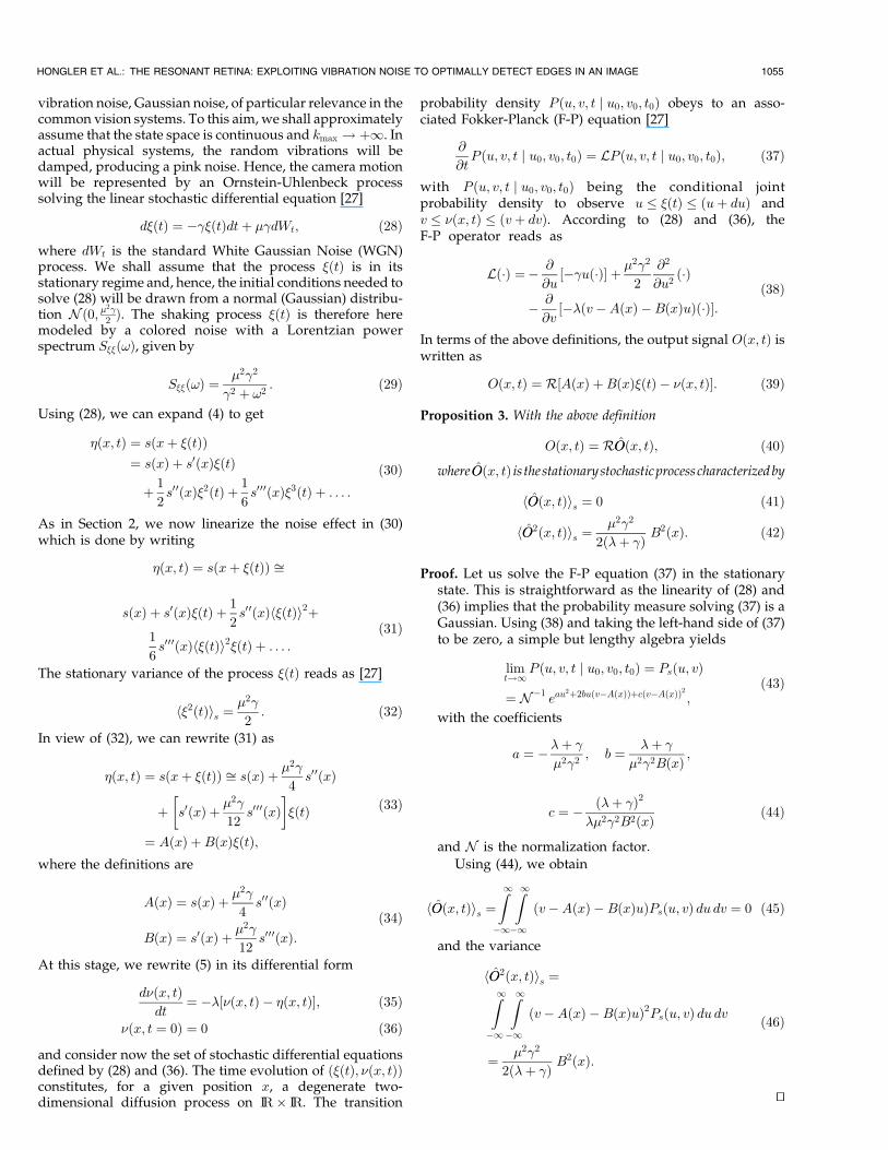
The behavior of (51) is represented in Figs. 1 and 2 as afunction of the threshold D and the output signal standarddeviation �o, where we clearly see the stochastic resonanceeffect. The Fisher information given by (51) shows a peakfor the ratio D

�o¼ 1:48. Thus, the optimum estimator

threshold D is linearly dependent on the standarddeviation of the output signal of the DR. The DR itself islinearly dependent on the standard deviation of thevibration noise and the magnitude gradient of the scene.

5 EXPERIMENTS

The concept of Resonant Retina (RR) that we haveintroduced integrates two separate elements, namely,

. the use of random motion of the optical axis of acamera as the basis for neighborhood style imagecomputations and

. the use of a threshold detector to estimate thevariance of a stationary process.

Clearly, to validate the overall concept of RR, “realworld” experiments have to be performed. Note first thatthe variance estimation of a stationary process by athreshold detector only requires standard data processingoperations. Simulation experiments, as those reportedbelow, already offer a proper validation procedure for suchdata processing. This however is simply not true for thecharacterization of the output signal delivered by an actualcamera subject to random vibrations. Note that such a “real

1056 IEEE TRANSACTIONS ON PATTERN ANALYSIS AND MACHINE INTELLIGENCE, VOL. 25, NO. 9, SEPTEMBER 2003

Fig. 1. For a Gaussian vibration the Fisher information, a measure of theestimator quality, shows a resonance peak. The maximum lies on theline given by D � 1:48�o.

Fig. 2. Fisher information as a function of the threshold D for four

different values of �o. There is an optimum threshold D � 1:48�o.

world” experiment is qualitatively reported in [1] whichprovides a preliminary feasibility of the DR concept. In [1],however, the authors do not offer a formal modeling of theDR concept and this is mandatory to quantify the influenceof the input parameters governing the DR. In the presentapproach, we definitely focus our attention to the modelingaspect of the problem. This clearly does not save us the taskto actually perform a “real world” experiment and this ispresently under realization. Such an experimental approachis indeed necessary to establish that, for a suitable range ofthe external control parameters, unavoidable elements thatdo not enter into our elementary model, indeed do notsignificantly affect the overall operation of the RR.

5.1 Experiments with the Threshold Estimator

The first group of experiments were conducted with thepurpose of studying the performance of the ThresholdEstimator (TE). Since each pixel works independently fromits neighbors, a single pixel has been used in a MATLABsimulation. To this end, a white Gaussian noise withstandard deviation � ¼ 2 was generated and fed to a TE.The noise sample has 100 values. The resulting estimation ofthe input standard deviation was averaged over 400 trials(realizations) and compared to the Mean Square Deviation(MSD) estimator.

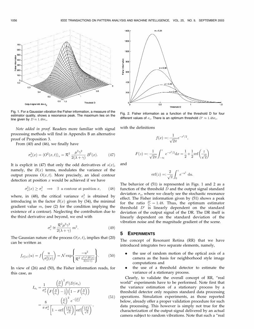
The results are shown in Fig. 3. Plotted in solid lines are theaverage values estimated by a TE with threshold D ¼ 2:96(the optimum, as shown at the end of Section 4) andD ¼ 1:0.The dotted and dashed lines correspond to the 68 percentconfidence intervals for TE with D ¼ 2:96 (-.-) , D ¼ 1:0 (- -),and the MSD estimator (� � � ).

The experiments show that the TE is an asymptoticallyunbiased estimator. Furthermore, the confidence interval issmallest for the MSD estimator, as it is considered the bestunbiased estimator for a Gaussian distribution. It can alsobe seen that the optimum threshold D ¼ 2:96 yields anarrower confidence interval compared to the TE withD ¼ 1. This shows that the Fisher information is indeedlarger for the resonance value D ¼ 2:96.

The second experiment compares the estimating cap-abilities of the TE for different threshold values. Thethresholds D ¼ 1; 2; 3, and 4 were chosen and the inputstandard deviation estimated during 100 iterations for aninput noise of � ¼ 2. The averages of 400 trials are shown inFig. 4. The stochastic resonance effect can clearly be seensince the estimators with threshold values clearly below(D ¼ 1) and above (D ¼ 4) the optimum are the slowest toconverge, that is, they have the highest variability.

5.2 Edge Detector Experiments

After convincing ourselves of the performance of the TE, weproceed on to test the actual Resonant Retina (RR)algorithm. Here, we consider not a single pixel but anarray of Dynamic Retina pixels with their associated TEs, allwith a common threshold D. As before, we have limitedourselves to 1D images.

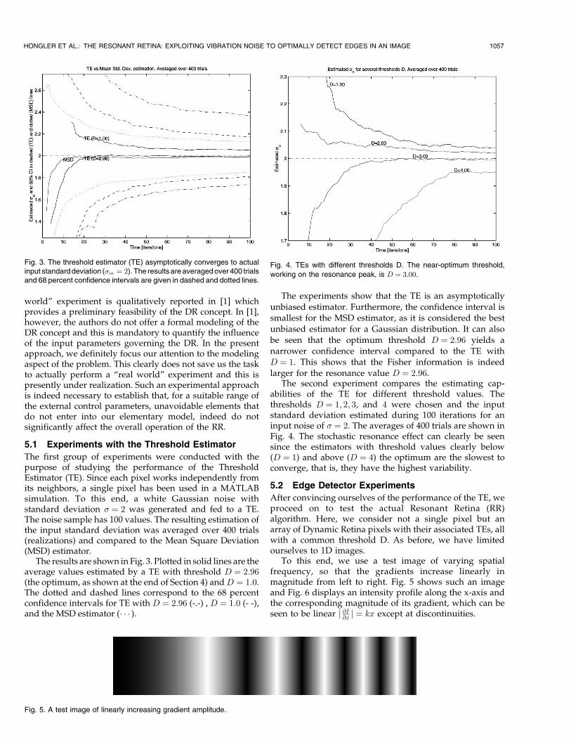
To this end, we use a test image of varying spatialfrequency, so that the gradients increase linearly inmagnitude from left to right. Fig. 5 shows such an imageand Fig. 6 displays an intensity profile along the x-axis andthe corresponding magnitude of its gradient, which can beseen to be linear j @I@x j ¼ kx except at discontinuities.

HONGLER ET AL.: THE RESONANT RETINA: EXPLOITING VIBRATION NOISE TO OPTIMALLY DETECT EDGES IN AN IMAGE 1057

Fig. 3. The threshold estimator (TE) asymptotically converges to actualinput standarddeviation (�in ¼ 2). The results are averagedover400 trialsand 68 percent confidence intervals are given in dashed and dotted lines.

Fig. 4. TEs with different thresholds D. The near-optimum threshold,

working on the resonance peak, is D ¼ 3:00.

Fig. 5. A test image of linearly increasing gradient amplitude.

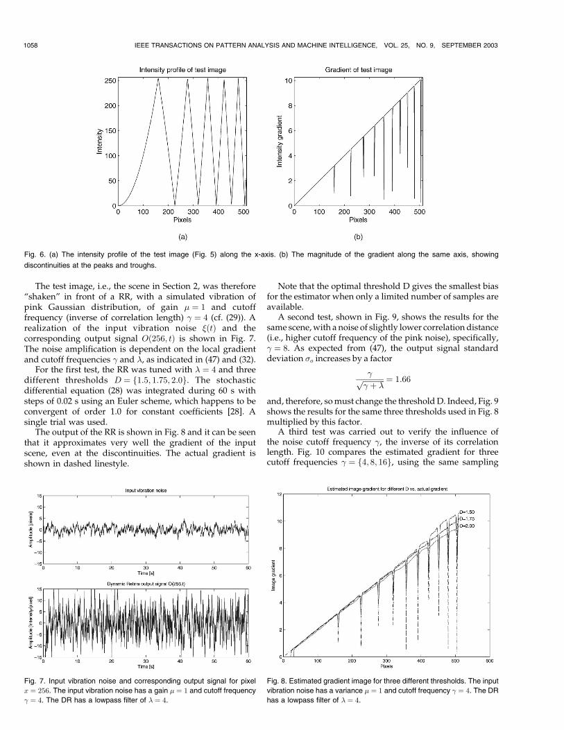
The test image, i.e., the scene in Section 2, was therefore“shaken” in front of a RR, with a simulated vibration ofpink Gaussian distribution, of gain � ¼ 1 and cutofffrequency (inverse of correlation length) � ¼ 4 (cf. (29)). Arealization of the input vibration noise �ðtÞ and thecorresponding output signal Oð256; tÞ is shown in Fig. 7.The noise amplification is dependent on the local gradientand cutoff frequencies � and �, as indicated in (47) and (32).

For the first test, the RR was tuned with � ¼ 4 and threedifferent thresholds D ¼ f1:5; 1:75; 2:0g. The stochasticdifferential equation (28) was integrated during 60 s withsteps of 0.02 s using an Euler scheme, which happens to beconvergent of order 1.0 for constant coefficients [28]. Asingle trial was used.

The output of the RR is shown in Fig. 8 and it can be seenthat it approximates very well the gradient of the inputscene, even at the discontinuities. The actual gradient isshown in dashed linestyle.

Note that the optimal threshold D gives the smallest biasfor the estimator when only a limited number of samples areavailable.

A second test, shown in Fig. 9, shows the results for thesame scene,with a noise of slightly lower correlation distance(i.e., higher cutoff frequency of the pink noise), specifically,� ¼ 8. As expected from (47), the output signal standarddeviation �o increases by a factor

�ffiffiffiffiffiffiffiffiffiffiffiffi� þ �

p ¼ 1:66

and, therefore, somust change the thresholdD. Indeed, Fig. 9shows the results for the same three thresholds used in Fig. 8multiplied by this factor.

A third test was carried out to verify the influence ofthe noise cutoff frequency �, the inverse of its correlationlength. Fig. 10 compares the estimated gradient for threecutoff frequencies � ¼ f4; 8; 16g, using the same sampling

1058 IEEE TRANSACTIONS ON PATTERN ANALYSIS AND MACHINE INTELLIGENCE, VOL. 25, NO. 9, SEPTEMBER 2003

Fig. 6. (a) The intensity profile of the test image (Fig. 5) along the x-axis. (b) The magnitude of the gradient along the same axis, showing

discontinuities at the peaks and troughs.

Fig. 7. Input vibration noise and corresponding output signal for pixel

x ¼ 256. The input vibration noise has a gain � ¼ 1 and cutoff frequency

� ¼ 4. The DR has a lowpass filter of � ¼ 4.

Fig. 8. Estimated gradient image for three different thresholds. The input

vibration noise has a variance � ¼ 1 and cutoff frequency � ¼ 4. The DR

has a lowpass filter of � ¼ 4.

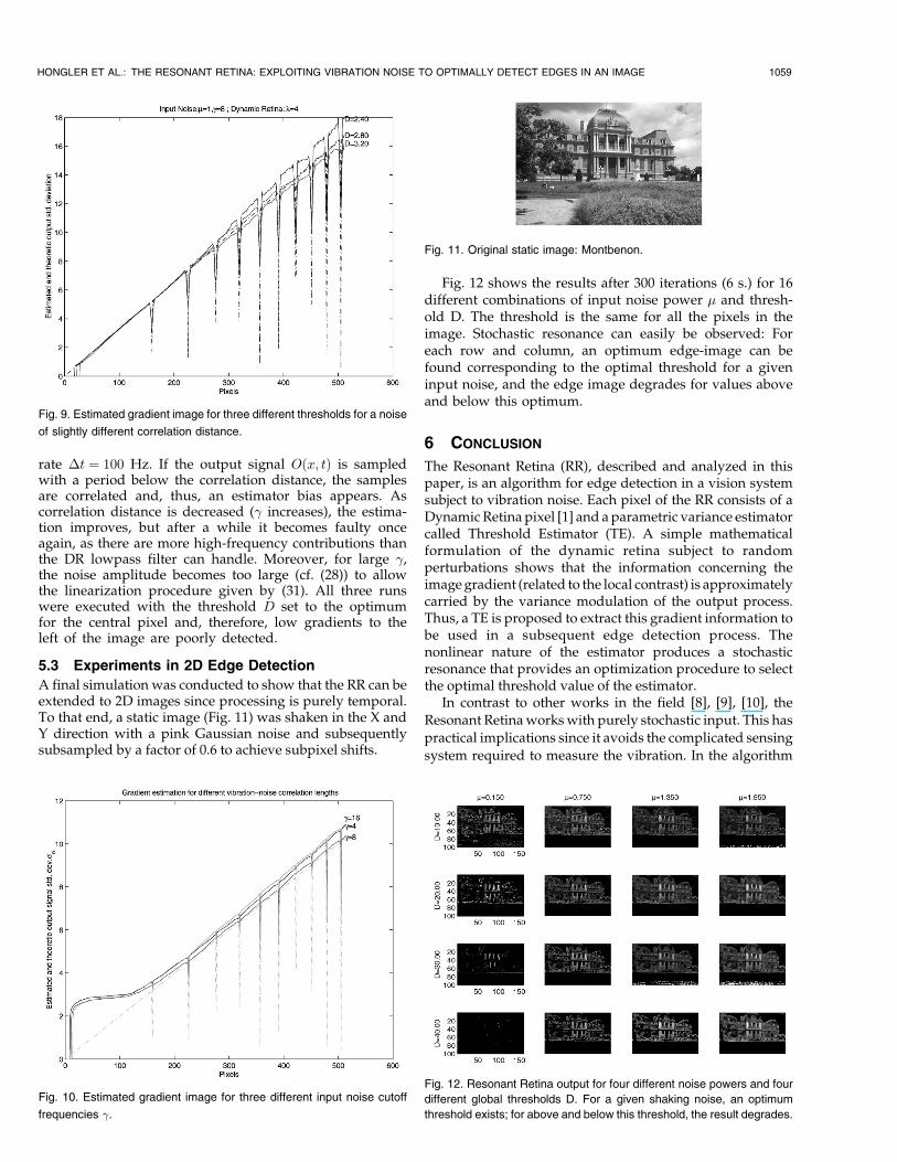
rate �t ¼ 100 Hz. If the output signal Oðx; tÞ is sampledwith a period below the correlation distance, the samplesare correlated and, thus, an estimator bias appears. Ascorrelation distance is decreased (� increases), the estima-tion improves, but after a while it becomes faulty onceagain, as there are more high-frequency contributions thanthe DR lowpass filter can handle. Moreover, for large �,the noise amplitude becomes too large (cf. (28)) to allowthe linearization procedure given by (31). All three runswere executed with the threshold D set to the optimumfor the central pixel and, therefore, low gradients to theleft of the image are poorly detected.

5.3 Experiments in 2D Edge Detection

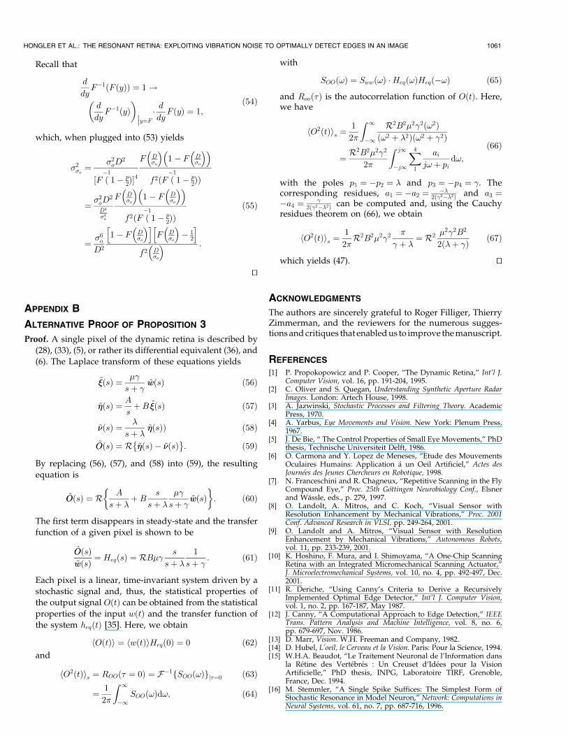
A final simulation was conducted to show that the RR can beextended to 2D images since processing is purely temporal.To that end, a static image (Fig. 11) was shaken in the X andY direction with a pink Gaussian noise and subsequentlysubsampled by a factor of 0.6 to achieve subpixel shifts.

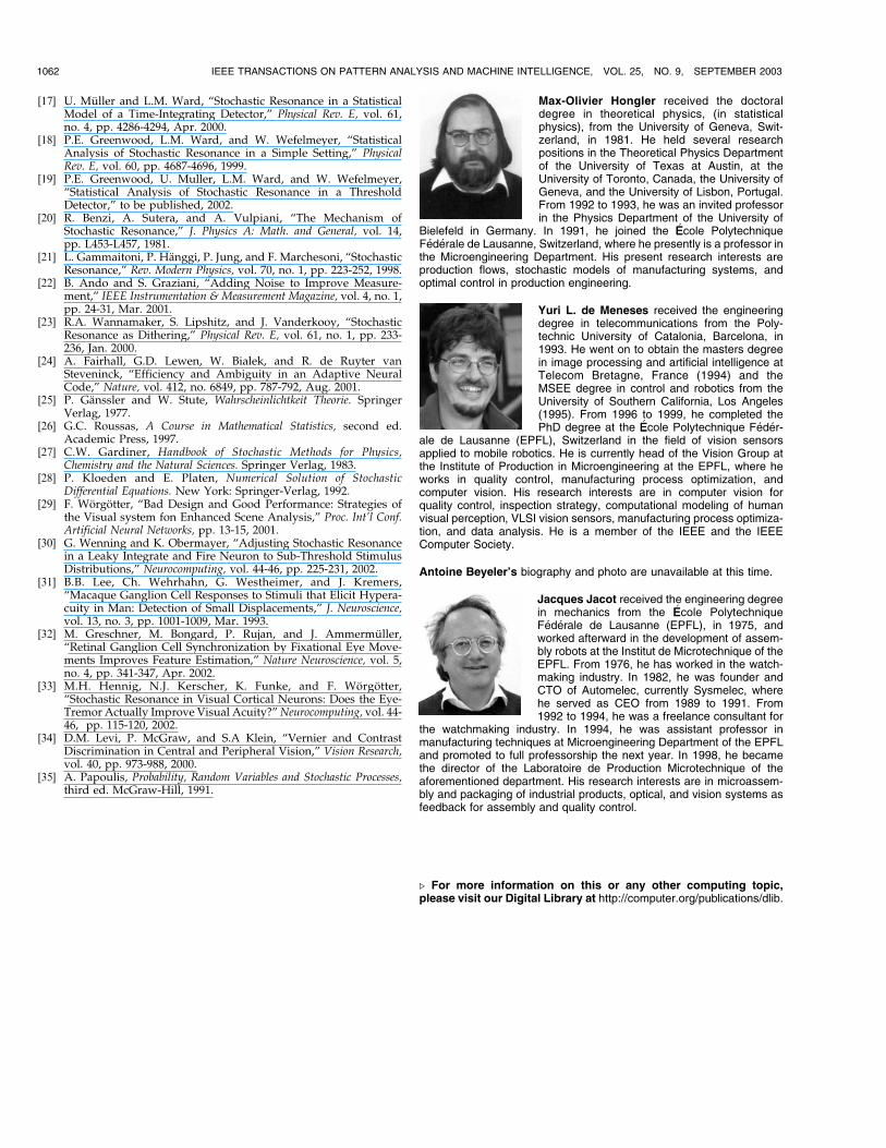
Fig. 12 shows the results after 300 iterations (6 s.) for 16different combinations of input noise power � and thresh-old D. The threshold is the same for all the pixels in theimage. Stochastic resonance can easily be observed: Foreach row and column, an optimum edge-image can befound corresponding to the optimal threshold for a giveninput noise, and the edge image degrades for values aboveand below this optimum.

6 CONCLUSION

The Resonant Retina (RR), described and analyzed in thispaper, is an algorithm for edge detection in a vision systemsubject to vibration noise. Each pixel of the RR consists of aDynamicRetina pixel [1] and a parametric variance estimatorcalled Threshold Estimator (TE). A simple mathematicalformulation of the dynamic retina subject to randomperturbations shows that the information concerning theimagegradient (related to the local contrast) is approximatelycarried by the variance modulation of the output process.Thus, a TE is proposed to extract this gradient information tobe used in a subsequent edge detection process. Thenonlinear nature of the estimator produces a stochasticresonance that provides an optimization procedure to selectthe optimal threshold value of the estimator.

In contrast to other works in the field [8], [9], [10], the

Resonant Retinaworkswith purely stochastic input. This has

practical implications since it avoids the complicated sensing

system required to measure the vibration. In the algorithm

HONGLER ET AL.: THE RESONANT RETINA: EXPLOITING VIBRATION NOISE TO OPTIMALLY DETECT EDGES IN AN IMAGE 1059

Fig. 9. Estimated gradient image for three different thresholds for a noise

of slightly different correlation distance.

Fig. 10. Estimated gradient image for three different input noise cutoff

frequencies �.

Fig. 11. Original static image: Montbenon.

Fig. 12. Resonant Retina output for four different noise powers and four

different global thresholds D. For a given shaking noise, an optimum

threshold exists; for above and below this threshold, the result degrades.

described in this contribution, only the first and second orderstatistics of the perturbation need to be known.

Wehavepurposefullyselectedanalgorithmthatallowsthesystem to adapt itself, so that it canbe rendered robust againsta changingenvironment—lighting changes, adynamic scene,or a different vibration noise. Three control parameters thatcan be freely tuned to match a wide range of operatingconditions.Namely, our explicit analysis of the role playedbythe cutoff frequency �, the output gain R, and the thresholdvalueD, canbeusedto tune thesystem.Furthermore,wehaveshowntheexistenceofanoptimumthresholdvalueforagiveninput vibration noise and how the Fisher information of theestimator can be used to find this optimum.

A promising contribution of this paper is the use of theThreshold Estimator (TE) to compute the variance of a signal,a tool also used in [18]. Note, however, that in [18] the TE isused to estimate the average of the signal. In our case, it is thevariance that is obtained by such a parametric estimator.

A key feature of the Resonant Retina is that each pixelcarries out a relatively simple computation, independentlyfrom its neighbors. It is thus particularly advantageous forVLSI implementations, both digital and analog [8]. In theanalog world, this translates into a massively parallelsystem—no communication is needed among pixels—ofsmall-size pixels. In the digital one, it means less memoryrequirements, simplified routing (e.g., in FPGA implemen-tations) and, specifically, for the TE that it can beimplemented in fixed-point processors.

Finally, it should be clear that, despite of the fact thatnoise contributes to information gathering in the DRsystem, obviously it does not add any additional informa-tion that is not already present in the original, static scene.Noise here merely plays the role of a “catalyst” in theinformation-gathering process. Yet, the resulting informa-tion is pertinent enough for the tasks that follow, namely,edge detection and object segmentation.

6.1 Biological Underpinnings

Although some elements of the Resonant Retina—vibratingnoise in form of microsaccades [29], [5], temporal bandpassprocessing on the outer plexiform layer of the retina [15], theThreshold Estimator [16], [17]—can be found in biologicalvision systems, it should be clear that the RR is not amodel ofbiological retinas, for it does not provide a structural nor acomplete functional descriptionof the latter. Inparticular, theRR lacks the spatial connections among “neurons” that arepresent in the vertebrate retina, and the resulting spatiotem-poral filtering in the vertebrate retina is nonseparable [15], afeature not covered in our system.

Rather than modeling the biological retina, this papersuggests an information-theoretic signal-processing ap-proach that is capable of handling the shaking noise.Particularly, we want to stress the fact that this can beachieved by local information that is available at eachprocessing unit or pixel, as in [30].

Note, finally, that there is physiological evidence thatStochastic Resonance is present in the visual pathway, inthe retinal ganglion cells of the inner plexiform layer asshown in [31] and [32] or in cortical areas [33]. SR seems toimprove visual acuity, that is, the resolving power of theganglion cells, which mediate in edge detection. Vernier

discrimination (acuity) and contrast discrimination seem tobe processed at the same site, namely, the ganglion cells[34]. As suggested by [31], it is probably spatial coherencethat affords the distinction between a change in edgeposition (Vernier acuity) and contrast change.

6.2 Perspectives

Not considering the ubiquitous presence of noise as anuisance but on the contrary, trying to use it as a tool in adetection process, is a not-so-common paradigm in theengineering methodology. This contribution inspired by thepioneering work [1], where the idea of a dynamic retina ispresented, has formally examined the possibility to use theubiquitous mechanical noise affecting a camera sensing on amobile platform, to detect the edges of the received images.

This contribution should be considered, from the point ofview of actual realizations, as in a preliminary stage.Indeed, our experimental approach was restricted tocomputer simulations. Real environments are likely togenerate new difficulties that have not yet been explored.However, as long as the noise amplitude remains relativelysmall, the overall procedure will certainly be robust.

APPENDIX A

PROOF OF PROPOSITION 2

Proof. For a large number n of experiments, the value ppðxÞwill converge with pðxÞ. Let us write

2 ¼ ppðxÞ � pðxÞ

and using (22) and (24), we can write

ffiffiffin

pð�o � ��oÞ

¼ffiffiffin

p D

F ð�1

1� p2Þ� D

F ð�1

1� pp2Þ

264

375

�ffiffiffin

p D

F ð�1

1� p2Þ� D

F ð�1

1� p2Þ þ d

dy F�1ðyÞjy¼1�p

2

264

375

�ffiffiffin

p D

F ð�1

1� p2Þ� D

F ð�1

1� p2Þ

1�

ddy F

�1ðyÞjy¼1�p2

F ð�1

1� p2Þ

264

375

264

375

¼ffiffiffin

p D

½F ð�1

1� p2Þ�

2

d

dyF�1ðyÞjy¼1�p

2

264

375 :

ð52Þ

Hence, for asymptotically large n, the variance of the

estimator in (52) is

�2�o

¼ D2

½F ð�1

1� p2Þ�

4

d

dyF�1ðyÞjy¼1�p

2

�2n < 2 >

¼ D2

½F ð�1

1� p2Þ

4�

d

dyF�1ðyÞjy¼1�p

2

�2

� 1� FD

�o

� �F

D

�o

� � 1

2

�� :

ð53Þ

1060 IEEE TRANSACTIONS ON PATTERN ANALYSIS AND MACHINE INTELLIGENCE, VOL. 25, NO. 9, SEPTEMBER 2003

Recall that

d

dyF�1ðF ðyÞÞ ¼ 1 !

d

dyF�1ðyÞ

� ��y¼F

� ddy

F ðyÞ ¼ 1;ð54Þ

which, when plugged into (53) yields

�2�o

¼ �2oD2

½F ð�1

1� p2Þ�

4

F D�o

� �1� F D

�o

� �� �

f2ðF ð�1

1� p2ÞÞ

¼ �2oD2

D4

�4o

F�D�o

��1� F

�D�o

��

f2ðF ð�1

1� p2ÞÞ

¼ �6o

D2

1� F D�o

� �h iF D

�o

� �� 1

2

h i

f2 D�o

� � :

ð55Þ

tu

APPENDIX B

ALTERNATIVE PROOF OF PROPOSITION 3

Proof. A single pixel of the dynamic retina is described by

(28), (33), (5), or rather its differential equivalent (36), and

(6). The Laplace transform of these equations yields

~��ðsÞ ¼ ��

sþ �~wwðsÞ ð56Þ

~��ðsÞ ¼ A

sþB ~��ðsÞ ð57Þ

~��ðsÞ ¼ �

sþ �~��ðsÞÞ ð58Þ

~OOðsÞ ¼ R�~��ðsÞ � ~��ðsÞ

�: ð59Þ

By replacing (56), (57), and (58) into (59), the resulting

equation is

~OOðsÞ ¼ R A

sþ �þB

s

sþ �

��

sþ �~wwðsÞ

� �: ð60Þ

The first term disappears in steady-state and the transfer

function of a given pixel is shown to be

~OOðsÞ~wwðsÞ ¼ HeqðsÞ ¼ RB��

s

sþ �

1

sþ �: ð61Þ

Each pixel is a linear, time-invariant system driven by a

stochastic signal and, thus, the statistical properties of

the output signal OðtÞ can be obtained from the statistical

properties of the input wðtÞ and the transfer function of

the system heqðtÞ [35]. Here, we obtain

hOðtÞi ¼ hwðtÞiHeqð0Þ ¼ 0 ð62Þand

hO2ðtÞis ¼ ROOð� ¼ 0Þ ¼ F�1 SOOð!Þf gj�¼0 ð63Þ

¼ 1

2�

Z 1

�1SOOð!Þd!; ð64Þ

with

SOOð!Þ ¼ Swwð!Þ �Heqð!ÞHeqð�!Þ ð65Þ

and Rooð�Þ is the autocorrelation function of OðtÞ. Here,we have

hO2ðtÞis ¼1

2�

Z 1

�1

R2B2�2�2ð!2Þð!2 þ �2Þð!2 þ �2Þ

¼ R2B2�2�2

2�

Z j1

�j1

X41

aij!þ pi

d!;

ð66Þ

with the poles p1 ¼ �p2 ¼ � and p3 ¼ �p4 ¼ �. Thecorresponding residues, a1 ¼ �a2 ¼ ��

2ð�2��2Þ and a3 ¼�a4 ¼ �

2ð�2��2Þ can be computed and, using the Cauchyresidues theorem on (66), we obtain

hO2ðtÞis ¼1

2�R2B2�2�2

�

� þ �¼ R2 �2�2B2

2ð�þ �Þ ð67Þ

which yields (47). tu

ACKNOWLEDGMENTS

The authors are sincerely grateful to Roger Filliger, ThierryZimmerman, and the reviewers for the numerous sugges-tionsandcritiques that enabledus to improve themanuscript.

REFERENCES

[1] P. Propokopowicz and P. Cooper, “The Dynamic Retina,” Int’l J.Computer Vision, vol. 16, pp. 191-204, 1995.

[2] C. Oliver and S. Quegan, Understanding Synthetic Aperture RadarImages. London: Artech House, 1998.

[3] A. Jazwinski, Stochastic Processes and Filtering Theory. AcademicPress, 1970.

[4] A. Yarbus, Eye Movements and Vision. New York: Plenum Press,1967.

[5] J. De Bie, “ The Control Properties of Small Eye Movements,” PhDthesis, Technische Universiteit Delft, 1986.

[6] O. Carmona and Y. Lopez de Meneses, “Etude des MouvementsOculaires Humains: Application a un Oeil Artificiel,” Actes desJournees des Jeunes Chercheurs en Robotique, 1998.

[7] N. Franceschini and R. Chagneux, “Repetitive Scanning in the FlyCompound Eye,” Proc. 25th Gottingen Neurobiology Conf., Elsnerand Wassle, eds., p. 279, 1997.

[8] O. Landolt, A. Mitros, and C. Koch, “Visual Sensor withResolution Enhancement by Mechanical Vibrations,” Proc. 2001Conf. Advanced Research in VLSI, pp. 249-264, 2001.

[9] O. Landolt and A. Mitros, “Visual Sensor with ResolutionEnhancement by Mechanical Vibrations,” Autonomous Robots,vol. 11, pp. 233-239, 2001.

[10] K. Hoshino, F. Mura, and I. Shimoyama, “A One-Chip ScanningRetina with an Integrated Micromechanical Scanning Actuator,”J. Microelectromechanical Systems, vol. 10, no. 4, pp. 492-497, Dec.2001.

[11] R. Deriche, “Using Canny’s Criteria to Derive a RecursivelyImplemented Optimal Edge Detector,” Int’l J. Computer Vision,vol. 1, no. 2, pp. 167-187, May 1987.

[12] J. Canny, “A Computational Approach to Edge Detection,” IEEETrans. Pattern Analysis and Machine Intelligence, vol. 8, no. 6,pp. 679-697, Nov. 1986.

[13] D. Marr, Vision. W.H. Freeman and Company, 1982.[14] D. Hubel, L’oeil, le Cerveau et la Vision. Paris: Pour la Science, 1994.[15] W.H.A. Beaudot, “Le Traitement Neuronal de l’Information dans

la Retine des Vertebres : Un Creuset d’Idees pour la VisionArtificielle,” PhD thesis, INPG, Laboratoire TIRF, Grenoble,France, Dec. 1994.

[16] M. Stemmler, “A Single Spike Suffices: The Simplest Form ofStochastic Resonance in Model Neuron,” Network: Computations inNeural Systems, vol. 61, no. 7, pp. 687-716, 1996.

HONGLER ET AL.: THE RESONANT RETINA: EXPLOITING VIBRATION NOISE TO OPTIMALLY DETECT EDGES IN AN IMAGE 1061

[17] U. Muller and L.M. Ward, “Stochastic Resonance in a StatisticalModel of a Time-Integrating Detector,” Physical Rev. E, vol. 61,no. 4, pp. 4286-4294, Apr. 2000.

[18] P.E. Greenwood, L.M. Ward, and W. Wefelmeyer, “StatisticalAnalysis of Stochastic Resonance in a Simple Setting,” PhysicalRev. E, vol. 60, pp. 4687-4696, 1999.

[19] P.E. Greenwood, U. Muller, L.M. Ward, and W. Wefelmeyer,“Statistical Analysis of Stochastic Resonance in a ThresholdDetector,” to be published, 2002.

[20] R. Benzi, A. Sutera, and A. Vulpiani, “The Mechanism ofStochastic Resonance,” J. Physics A: Math. and General, vol. 14,pp. L453-L457, 1981.

[21] L. Gammaitoni, P. Hanggi, P. Jung, and F. Marchesoni, “StochasticResonance,” Rev. Modern Physics, vol. 70, no. 1, pp. 223-252, 1998.

[22] B. Ando and S. Graziani, “Adding Noise to Improve Measure-ment,” IEEE Instrumentation & Measurement Magazine, vol. 4, no. 1,pp. 24-31, Mar. 2001.

[23] R.A. Wannamaker, S. Lipshitz, and J. Vanderkooy, “StochasticResonance as Dithering,” Physical Rev. E, vol. 61, no. 1, pp. 233-236, Jan. 2000.

[24] A. Fairhall, G.D. Lewen, W. Bialek, and R. de Ruyter vanSteveninck, “Efficiency and Ambiguity in an Adaptive NeuralCode,” Nature, vol. 412, no. 6849, pp. 787-792, Aug. 2001.

[25] P. Ganssler and W. Stute, Wahrscheinlichtkeit Theorie. SpringerVerlag, 1977.

[26] G.C. Roussas, A Course in Mathematical Statistics, second ed.Academic Press, 1997.

[27] C.W. Gardiner, Handbook of Stochastic Methods for Physics,Chemistry and the Natural Sciences. Springer Verlag, 1983.

[28] P. Kloeden and E. Platen, Numerical Solution of StochasticDifferential Equations. New York: Springer-Verlag, 1992.

[29] F. Worgotter, “Bad Design and Good Performance: Strategies ofthe Visual system fon Enhanced Scene Analysis,” Proc. Int’l Conf.Artificial Neural Networks, pp. 13-15, 2001.

[30] G. Wenning and K. Obermayer, “Adjusting Stochastic Resonancein a Leaky Integrate and Fire Neuron to Sub-Threshold StimulusDistributions,” Neurocomputing, vol. 44-46, pp. 225-231, 2002.

[31] B.B. Lee, Ch. Wehrhahn, G. Westheimer, and J. Kremers,“Macaque Ganglion Cell Responses to Stimuli that Elicit Hypera-cuity in Man: Detection of Small Displacements,” J. Neuroscience,vol. 13, no. 3, pp. 1001-1009, Mar. 1993.

[32] M. Greschner, M. Bongard, P. Rujan, and J. Ammermuller,“Retinal Ganglion Cell Synchronization by Fixational Eye Move-ments Improves Feature Estimation,” Nature Neuroscience, vol. 5,no. 4, pp. 341-347, Apr. 2002.

[33] M.H. Hennig, N.J. Kerscher, K. Funke, and F. Worgotter,“Stochastic Resonance in Visual Cortical Neurons: Does the Eye-Tremor Actually Improve Visual Acuity?”Neurocomputing, vol. 44-46, pp. 115-120, 2002.

[34] D.M. Levi, P. McGraw, and S.A Klein, “Vernier and ContrastDiscrimination in Central and Peripheral Vision,” Vision Research,vol. 40, pp. 973-988, 2000.

[35] A. Papoulis, Probability, Random Variables and Stochastic Processes,third ed. McGraw-Hill, 1991.

Max-Olivier Hongler received the doctoraldegree in theoretical physics, (in statisticalphysics), from the University of Geneva, Swit-zerland, in 1981. He held several researchpositions in the Theoretical Physics Departmentof the University of Texas at Austin, at theUniversity of Toronto, Canada, the University ofGeneva, and the University of Lisbon, Portugal.From 1992 to 1993, he was an invited professorin the Physics Department of the University of

Bielefeld in Germany. In 1991, he joined the �EEcole PolytechniqueFederale de Lausanne, Switzerland, where he presently is a professor inthe Microengineering Department. His present research interests areproduction flows, stochastic models of manufacturing systems, andoptimal control in production engineering.

Yuri L. de Meneses received the engineeringdegree in telecommunications from the Poly-technic University of Catalonia, Barcelona, in1993. He went on to obtain the masters degreein image processing and artificial intelligence atTelecom Bretagne, France (1994) and theMSEE degree in control and robotics from theUniversity of Southern California, Los Angeles(1995). From 1996 to 1999, he completed thePhD degree at the �EEcole Polytechnique Feder-

ale de Lausanne (EPFL), Switzerland in the field of vision sensorsapplied to mobile robotics. He is currently head of the Vision Group atthe Institute of Production in Microengineering at the EPFL, where heworks in quality control, manufacturing process optimization, andcomputer vision. His research interests are in computer vision forquality control, inspection strategy, computational modeling of humanvisual perception, VLSI vision sensors, manufacturing process optimiza-tion, and data analysis. He is a member of the IEEE and the IEEEComputer Society.

Antoine Beyeler’s biography and photo are unavailable at this time.

Jacques Jacot received the engineering degreein mechanics from the �EEcole PolytechniqueFederale de Lausanne (EPFL), in 1975, andworked afterward in the development of assem-bly robots at the Institut de Microtechnique of theEPFL. From 1976, he has worked in the watch-making industry. In 1982, he was founder andCTO of Automelec, currently Sysmelec, wherehe served as CEO from 1989 to 1991. From1992 to 1994, he was a freelance consultant for

the watchmaking industry. In 1994, he was assistant professor inmanufacturing techniques at Microengineering Department of the EPFLand promoted to full professorship the next year. In 1998, he becamethe director of the Laboratoire de Production Microtechnique of theaforementioned department. His research interests are in microassem-bly and packaging of industrial products, optical, and vision systems asfeedback for assembly and quality control.

. For more information on this or any other computing topic,please visit our Digital Library at http://computer.org/publications/dlib.

1062 IEEE TRANSACTIONS ON PATTERN ANALYSIS AND MACHINE INTELLIGENCE, VOL. 25, NO. 9, SEPTEMBER 2003