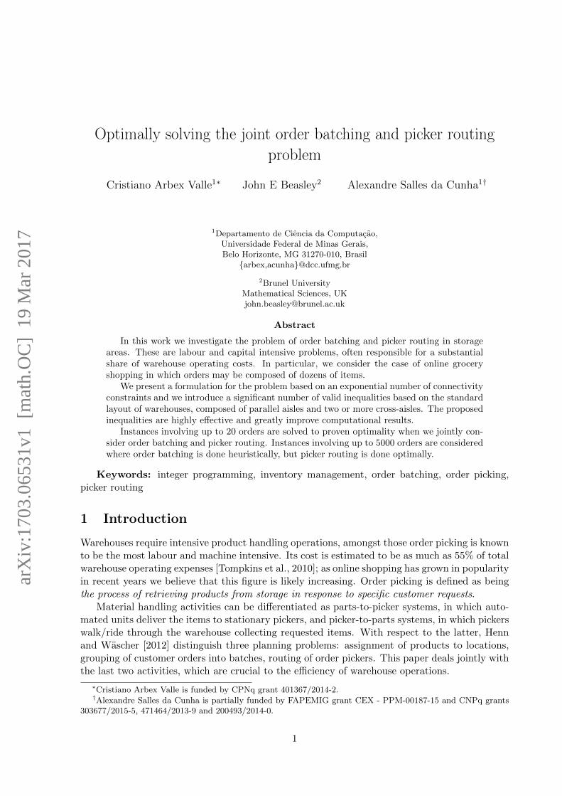
Optimally solving the joint order batching and picker routing

problem

Cristiano Arbex Valle1∗ John E Beasley2 Alexandre Salles da Cunha1†

1Departamento de Ciencia da Computacao,Universidade Federal de Minas Gerais,Belo Horizonte, MG 31270-010, Brasilarbex,acunha@dcc.ufmg.br

2Brunel UniversityMathematical Sciences, UKjohn.beasley@brunel.ac.uk

Abstract

In this work we investigate the problem of order batching and picker routing in storageareas. These are labour and capital intensive problems, often responsible for a substantialshare of warehouse operating costs. In particular, we consider the case of online groceryshopping in which orders may be composed of dozens of items.

We present a formulation for the problem based on an exponential number of connectivityconstraints and we introduce a significant number of valid inequalities based on the standardlayout of warehouses, composed of parallel aisles and two or more cross-aisles. The proposedinequalities are highly effective and greatly improve computational results.

Instances involving up to 20 orders are solved to proven optimality when we jointly con-sider order batching and picker routing. Instances involving up to 5000 orders are consideredwhere order batching is done heuristically, but picker routing is done optimally.

Keywords: integer programming, inventory management, order batching, order picking,picker routing

1 Introduction

Warehouses require intensive product handling operations, amongst those order picking is knownto be the most labour and machine intensive. Its cost is estimated to be as much as 55% of totalwarehouse operating expenses [Tompkins et al., 2010]; as online shopping has grown in popularityin recent years we believe that this figure is likely increasing. Order picking is defined as beingthe process of retrieving products from storage in response to specific customer requests.

Material handling activities can be differentiated as parts-to-picker systems, in which auto-mated units deliver the items to stationary pickers, and picker-to-parts systems, in which pickerswalk/ride through the warehouse collecting requested items. With respect to the latter, Hennand Wascher [2012] distinguish three planning problems: assignment of products to locations,grouping of customer orders into batches, routing of order pickers. This paper deals jointly withthe last two activities, which are crucial to the efficiency of warehouse operations.

∗Cristiano Arbex Valle is funded by CPNq grant 401367/2014-2.†Alexandre Salles da Cunha is partially funded by FAPEMIG grant CEX - PPM-00187-15 and CNPq grants

303677/2015-5, 471464/2013-9 and 200493/2014-0.

1

arX

iv:1

703.

0653

1v1

[m

ath.

OC

] 1

9 M

ar 2

017

In particular, we consider the case of online grocery shopping, where orders may be composedof dozens of items. As practical aspects of this problem we highlight (i) the heterogeneity ofproducts (which can be of various shapes, sizes or expiration dates) and (ii) the fact that thepicking can be performed in warehouses that are either closed or open to the public (suchas supermarkets); due to such features pickers generally walk/ride the warehouse, collectingproducts manually instead of relying on automated systems. Pickers place products in baskets;when orders can be composed of dozens of items, mixing different orders in the same basket orsplitting an order among different pickers is generally avoided to reduce order processing errors.

We formulate and solve the Joint Order Batching and Picker Routing Problem (JOBPRP).The task is to find minimum-cost closed walks where each picker visits all locations requiredto pick all products from their assigned orders. Locations may be visited more than once ifnecessary. In our previous work [Valle et al., 2016] we introduced three integer programmingformulations for JOBPRP, each one being the basis for a different branch-and-bound algorithm.One of the formulations is a directed model that involves exponentially many constraints toenforce connectivity requirements for closed walks. The other two are compact formulationsbased on network flows. We introduced a branch-and-cut algorithm that relies on the non-compact model and examined the compact formulations using the CPLEX branch-and-boundsolver. Results suggested that the non-compact formulation and the compact formulation basedon single-commodity network flows are competitive. In our experiments, the formulation basedon multi-commodity flows ran out of memory for larger instances.

In this work, we focus on an improved version of the non-compact formulation. Our maincontribution is the introduction of several valid inequalities (cuts) based on a sparse graphrepresentation of warehouses which, to the best of our knowledge, have never been proposedbefore. We show that the inclusion of these cuts in the non-compact formulation greatly improvescomputational results. The proposed cuts prevent many solutions that violate subtour breakingconstraints and thus the (relatively) expensive max-flow separation algorithm can be switchedoff. Moreover, if the batching and routing problems are solved separately, we show that, givenan assignment of orders to pickers, an optimal routing can be computed very quickly. We alsointroduce a special case of the problem where pickers are only allowed to reverse at corners,which is more intuitive for humans, reduces computation times and still produces solutions ofvery good quality when compared to the original problem.

As in Valle et al. [2016], we also introduce a JOBPRP test instance generator partially basedon publicly available real-world data. The test instances used in this work are available fordownload1.

The remainder of this paper is organised as follows. Section 2 presents a description and aliterature review of the problem. Section 3 introduces JOBPRP as a graph optimisation prob-lem and Section 4 presents the aforementioned non-compact integer programming formulationand briefly discusses some implementation details. Section 5 introduces several classes of validinequalities based on the standard layout of warehouses. Section 6 discusses computationalresults whilst Section 7 discusses the application of the approach in this paper in the contextof supermarket home deliveries. Finally in Section 8 we present some concluding remarks andfuture research directions.

2 Problem description and literature review

A warehouse has a rectangular layout with no unused space and consists of parallel aisles. Thewarehouse is divided into a number of blocks. Blocks are separated by cross-aisles. A subaisle

1Test instances available at http://www.dcc.ufmg.br/∼arbex/orderpicking.html

2

is defined as a section of an aisle within a block. Every warehouse has at least one cross-aisle atthe top and one at the bottom, but may contain more. Figure 1 illustrates these concepts.

Aisles contain slots on both sides, each slot holds one type of product. Slots can also bestacked vertically in shelves. We assume that pickers move in the centre of an aisle and thatproducts on both sides can be reached by the picker.

Figure 1: Warehouse structure

Figure 2: Example of warehouse/graph layout Figure 3: Warehouse with reduced graph

A typical warehouse layout with three cross-aisles, three aisles and two shelves, togetherwith a sparse graph representation, can be seen in Figure 2. White vertices represent locationsfrom where the picker reaches products, i.e. from the top left white vertex the picker reachesproducts in slots 1, 2, 19 and 20. Note here that whilst in Figure 2 we have shown just two slots

3

on each side of an aisle this is purely for ease of illustration. Our approach is not dependent onthe number of such slots and can be applied without modification to problems with more slots.

In Figure 2 there are six subaisles, each consisting of four consecutive white vertices. Blackvertices represent “artificial” locations which connect aisles and cross-aisles, while the “Origin”indicates the starting and return point for pickers. Often, however, not all locations need tobe visited as the joint set of orders does not contain products in all locations. It is thereforepossible to reduce the graph that depicts the warehouse by eliminating such locations, as it canbe seen in Figure 3, where, for example, no products in slots 3, 4, 21 and 22 are needed.

Pickers use trolleys that accommodate a limited number of baskets2. The number of basketsnecessary to carry each order is assumed to be known. In fact, in this work, we consider thatall baskets carry a fixed number of items, irrespective of their shapes and sizes. Baskets neededto carry a batch must not exceed trolley capacity. Following general practice in supermarkets,orders from different customers cannot be put together in the same basket and a single ordercannot be split between different trolleys. Mixing and dividing orders could reduce picking time,however this benefit is often offset by necessary post-processing and a higher risk of errors.

There is a vast literature on the problems of order batching and picking. An extensivesurvey relating to different picking strategies was presented by De Koster et al. [2007], whereorder picking is shown to be the most critical activity for productivity growth in the sector.Wave picking is an example of an alternative manual picking strategy, where the warehouse isdivided into zones, each zone being assigned to one or more pickers; however in this strategypost-processing of orders is necessary. In this paper we deal with batch picking, where a pickercollects all of the products for one or more orders.

The special case where a single picker is sufficient to collect all orders is a particular case ofthe Travelling Salesman Problem (TSP). Ratliff and Rosenthal [1983] showed that for warehouseswhich have only two cross-aisles (so a single block), the problem can be solved polynomially viaa dynamic programming approach. The algorithm by Ratliff & Rosenthal is based on a sparsegraph representation of the problem, whereas previous works on the TSP generally assumeda complete graph. The sparse graph representing a warehouse containing a single block is atype of series parallel graph. Cornuejols et al. [1985] generalised the algorithm by Ratliff &Rosenthal and showed that the TSP in any series parallel graph is solvable in polynomial time.In that work, the authors coined the term Graphical TSP (GTSP) to characterise the TSPproblem on sparse graphs - a major difference being that arcs and vertices can be revisited in atour, unlike the TSP in a complete graph. Fonlupt and Naddef [1992] showed that the GTSP ispolynomially solvable whenever the corresponding graph is TSP-perfect: in such graphs the TSPsubtour formulation defines the convex hull of all vectors that satisfy the TSP requirements, andthus the solution to its linear relaxation is integer. The authors also showed that series parallelgraphs are not TSP-perfect despite the GTSP being efficiently solvable in such graphs. Fonluptand Nachef [1993] extended these results by defining a generalisation of the TSP which, togetherwith dynamic programming techniques, is used to show that the GTSP is polynomially solvableon a broader class of graphs (such as Halin graphs [Cornuejols et al., 1983]).

Unlike Ratliff & Rosenthal, we assume that warehouses may be composed of multiple blocks.We however adopt the same representation as the corresponding graph is composed of seriesparallel subgraphs joined by paths of edges that represent cross-aisles. Figures 2 and 3 illustratethis as each block individually forms a single series parallel graph, however these two subgraphsare joined by the middle cross-aisle. Unlike Ratliff & Rosenthal, we also assume that from thesource one can reach any of the artificial vertices in the top cross-aisle. To the best of ourknowledge, the GTSP in graphs composed of several connected series parallel subgraphs, such

2In different industries, the terms cart and tote are more often used than trolley and basket.

4

as warehouses with multiple blocks, has not been shown to be efficiently solvable.A valid tour for a single picker includes vertices that must be visited and vertices that

may be visited. This is due to the existence of artificial vertices and the fact that pickers ingeneral are responsible for collecting a subset of orders which may not span the entire set ofnon-artificial vertices. For a single picker, the problem of finding the shortest walk which visits aknown required subset of vertices is known as the Steiner TSP (STSP) and was first studied byCornuejols et al. [1985], Fleischmann [1985], Orloff [1974]. Several formulations for the STSP,including compact ones, were proposed by Letchford et al. [2013]. The compact formulationsintroduced in Valle et al. [2016] were inspired by similar formulations introduced in [Letchfordet al., 2013].

When trolley capacity and multiple pickers are considered, the problem is similar to theSteiner Capacitated VRP (SCVRP) [Letchford and Oukil, 2006]. To the best of our knowledgeno work in the literature has attempted to solve it directly, although many algorithms have beendeveloped for similar problems such as the Capacitated VRP [Naddef, 2007, Fukasawa et al.,2006] and the Capacitated Arc Routing Problem [Belenguer and Benavent, 1998, Letchford andOukil, 2009]. A closely related problem is the Mixed-Capacitated General Routing Problem(MCGRP), which reduces to the SCVRP if the set of required arcs is empty. Bosco et al.[2013] and Irnich et al. [2015] proposed branch-and-cut algorithms for the MCGRP, althoughthe authors did not experiment on SCVRP instances (all instances had required arcs).

An important difference between SCVRP and JOBPRP however is that the indivisibility oforders must be respected; an order being assigned to a trolley implies that a group of verticesmust be visited (assuming each item can be picked at just one vertex). SCVRP is a special caseof JOBPRP whenever each order contains just a single product.

Many heuristics have been proposed for the problem of routing a single picker in warehouseswith multiple blocks. An evaluation of several heuristics is given by Petersen II [1997]. Roodber-gen and de Koster [2001b] introduced a dynamic programming algorithm for picker routing inwarehouses with up to three cross-aisles and Roodbergen and de Koster [2001a] presented heuris-tics for warehouses with multiple cross-aisles. The latter is compared to a branch-and-boundalgorithm based on a classical TSP formulation of the problem, which assumes a Hamiltoniancircuit in a complete graph where all vertices must be visited exactly once (no artificial verticesare considered). Theys et al. [2010] adapted the TSP LKH heuristic by Lin and Kernighan [1973]for single-picker routing and Dekker et al. [2004] studied the case of a Dutch retail companywhose layout is composed of multiple cross-aisles, two floors and different origin and destinationpoints for the pickers.

Several heuristics have also been proposed for batching and routing multiple pickers. Veryoften, routing distances are estimated using single-picker heuristics during the solution of thebatching problem. Henn et al. [2012] includes an extensive survey of batching methods.

For warehouses with two cross-aisles, a VNS heuristic was proposed by Albareda-Sambolaet al. [2009] and Tabu Search and Hill Climbing heuristics were introduced by Henn and Wascher[2012]. The latter methods were adapted by Henn and Schmid [2013] to a problem that alsoconsiders order sequencing. Azadnia et al. [2013] proposed heuristics that solve sequencing andbatching first, then routing in a second stage. For warehouses with three cross-aisles, Matusiaket al. [2014] proposed a simulated annealing algorithm which includes precedence constraints (forinstance, a heavier box has to be at the bottom of a container); routing of candidate batches issolved with the A*-algorithm from Hart et al. [1968].

For general warehouses with any number of blocks, several batching methods are presentedby de Koster et al. [1999], where routing distances are estimated using single-picker methods.Gibson and Sharp [1992] introduced batching heuristics based on two and four-dimensionalspace-filling curves. A genetic algorithm that jointly considers both routing and batching was

5

proposed by Hsu et al. [2004]. Lam et al. [2014] introduced an integer programming formulationfor batching, where routing distances are estimated. The problem is solved with a heuristicbased on fuzzy logic. An association-based clustering approach to batching considering customerdemands (instead of routing distance) is presented by Chen and Wu [2004].

As far as we are aware, very few exact algorithms for the joint batching and routing problemhave been proposed in the literature to date. The work presented here builds upon our previouswork [Valle et al., 2016], as discussed elsewhere in this paper. Hong et al. [2012b] presented aformulation that depends on explicitly enumerating all possible picker routes. No computationalresults for that formulation were presented, rather lower bounds on the solution to that formu-lation were developed as well as a heuristic procedure. Hong et al. [2012a] dealt with multiplepickers and a single block (so just two cross-aisles). They considered aisle congestion wherepickers are delayed by the presence of other pickers in the same aisle. In terms of picker routingthey considered each picker to follow the same route around all of the aisles, with the provisothat some aisles can be skipped if desirable. Hong et al. [2016] built on Hong et al. [2012a]and considered the situation when the pickers operate in a bucket brigade manner. In such asystem each trolley (equivalently bucket) follows the same route around all of the aisles, beingpassed from picker to picker along the route. Schloz et al. [2016] dealt with just a single pickerand a single block (so just two cross-aisles). Although they indicated that their approach canbe extended to more than one block, no numerical results were given. Unlike these works, theexact algorithm proposed here is general in the sense that it can be applied to warehouses withany number of blocks.

3 The joint problem of order batching and picker routing: agraph optimisation problem

Let P be the set of products whose storage slots in the warehouse are known and L be theset of locations in the warehouse from where a picker can collect products, i.e. the middle ofan aisle containing products on both sides, in different shelves, and from where the picker canreach those products. Each location L ∈ L contains a subset of products. A warehouse graphrepresentation includes a vertex for every location, represented by the white vertices in Figure2.

Let O be the set of orders that must be collected. Each order o ∈ O contains a subset ofproducts Po ⊆ P. Accordingly, for each order o ∈ O, the subset of locations Lo ⊆ L contains allproducts in Po - it is possible that multiple products of the same order are in a single location.L(O) =

⋃o∈O Lo represents the set of locations that contains all products that need to be picked

in all orders. Also let dlm ≥ 0 be the distance between locations l,m ∈ L, symmetric so thatdlm = dml.

In practice, very often L(O) 6= L, i.e. there are locations for which none of their prod-ucts are present in any of the outstanding orders. In such cases, the graph that represents awarehouse can be reduced by eliminating all vertices that represent locations in L \ L(O). Anexample of such reduced graph can be seen in Figure 3, where several vertices were removed asdiscussed previously. If v is eliminated, and there are arcs (u, v), (v, u), (w, v), (v, w), we createarcs (u,w), (w, u) where duw = dwu = duv + dvw = dwv + dvu.

Let T denote the set of available pickers (or trolleys), T = |T |, B be the number of basketsthat a trolley can carry and bo be the known number of baskets needed to carry order o ∈ O.We assume that a basket will only contain products from a single order, even if it is partiallyempty, i.e., it is not possible to put products of different orders in the same basket. Finally,let s be the origin point from where the trolleys depart (and to where they must return), and

6

accordingly let dsl ≥ 0 be the distance between location l and s.To define JOBPRP, we introduce a directed and connected graph D = (V,A). The set of

vertices V is given by the union of s (the origin point), a set V (O) containing a vertex for everylocation l ∈ L(O) and a set VA of “artificial locations”. These artificial locations are placedin corners between aisles and cross-aisles and do not contain products that must be picked.We also define sets Vo containing a vertex for every location l ∈ Lo,

⋃o∈O Vo = V (O). Thus,

V = s ∪ V (O) ∪ VA and |V | = 1 + |V (O)|+ |VA|. In Figure 3, the origin represents s, the 17white vertices represent V (O) and the 9 black vertices represent VA.

Given a vertex i ∈ V (O), define l(i) : V (O) → L(O) as the location to which the vertexrefers. Arcs in set A connect two neighbour vertices of V . For instance, arc (i, j) connectslocation l(i) to location l(j). dl(i),l(j) ≥ 0 represents the distance between vertices i and j. Forreadability we write dij instead of dl(i),l(j).

A solution to JOBPRP in D is a collection of T ∗ ≤ T closed walks, one for each trolley.Each closed walk t = 1, . . . , T ∗ is associated with a subgraph (Vt ∪ s, At) of D. Each walkstarts at s, traverses a set At ⊆ A of selected arcs and returns to s. For each t = 1, . . . , T ∗, letOt ⊆ O denote the subset of orders collected during walk t.

The following requirements must be met by solutions to JOBPRP:

• Capacity constraints impose that, for every t = 1, . . . , T ∗,∑

o∈Otbo ≤ B.

• Indivisibility of the products Po in each order o ∈ Ot collected by each trolley imposesthat, for every o ∈ Ot, there exists at least one walk t where if i ∈ Vt : l(i) ∈ Lo, thenevery j : l(j) ∈ Lo must also be visited by t, i.e., j ∈ Vt.

• Finally, in order to guarantee that the T ∗ walks collect all orders, we must impose that∪T ∗t=1Ot = O. We assume that there are at least as many orders as there are trolleysavailable.

JOBPRP is then the problem of finding T ∗ ≤ T closed walks, meeting the requirementsoutlined above, in order to minimize the total length

∑T ∗

t=1

∑(i,j)∈At

dij .As D is modelled as a sparse graph, vertices in V (O) have only two neighbours while those

in VA do not connect to more than four other vertices. A feasible trolley walk for JOBPRP maybe forced to not only repeat vertices but also to visit vertices from non-collected orders. Forinstance, this could occur if a product from a non-collected order happens to be between twodistinct products in a collected order. However, under reasonable assumptions, we can provethat the optimal solution to JOBPRP is composed of walks that may repeat vertices, but willnot repeat arcs. An explicit proof can be found in the appendix of Letchford and Oukil [2009],for a closely related problem.

Lemma 1. Let us assume that D is such that for every arc (i, j) there is a corresponding arc(j, i) and that dij = dji ≥ 0. Then, in the optimal solution T ∗ to JOBPRP, every walk t ∈ T ∗visits each arc in At exactly once.

4 An integer programming formulation for the JOBPRP

Based on Lemma 1, we introduce an integer programming formulation for the JOBPRP. Theformulation allows vertices to be visited multiple times, but enforces the condition that each arccannot be traversed more than once. The model uses exponentially many constraints to enforceconnectivity of the closed walks.

The formulation uses binary decision variables zot to indicate whether (zot = 1) or not(zot = 0) trolley t picks order o ∈ O, xtij to indicate whether (xtij = 1) or not (xtij = 0) arc

7

(i, j) ∈ A is traversed by trolley t, αt to indicate whether (αt = 1) or not (αt = 0) trolley t picksat least one order and yti to indicate whether (yti = 1) or not (yti = 0) vertex i ∈ V \ s isvisited by trolley t. In addition, the model uses variables gti ∈ Z+ to indicate the outdegree ofvertex i ∈ V in the closed walk for trolley t.

Let δ−(W ) = (i, j) ∈ A : i 6∈ W, j ∈ W, δ+(W ) = (i, j) ∈ A : i ∈ W, j 6∈ W andA(W ) = (i, j) ∈ A : i ∈ W, j ∈ W. Also, let |δ+(i)| be the maximum outdegree of i ∈ V (forsimplicity we write δ+(i) instead of δ+(i)). JOBPRP can be stated as the following IntegerProgram:

min∑t∈T

∑(i,j)∈A

dijxtij (1)

subject to:

∑o∈O

bozot ≤ Bαt, ∀t ∈ T (2)∑t∈T

zot = 1, ∀o ∈ O (3)∑(i,j)∈δ+(i)

xtij ≥ zot, ∀o ∈ O, t ∈ T , i : l(i) ∈ Lo, (4)

∑(i,j)∈δ+(i)

xtij =∑

(j,i)∈δ−(i)

xtji, ∀i ∈ V, t ∈ T (5)

∑(s,j)∈δ+(s)

xtsj =∑

(j,s)∈δ−(s)

xtjs = αt, ∀t ∈ T (6)

xtij ≤ αt, ∀(i, j) ∈ A, t ∈ T (7)

zot ≤ αt, ∀o ∈ O, t ∈ T (8)∑o∈O

zot ≥ αt, t ∈ T (9)∑(i,j)∈δ+(i)

xtij = gti, ∀i ∈ V, t ∈ T (10)

yti ≥ xtij , ∀(i, j) ∈ A, t ∈ T (11)∑j∈W

gtj ≥ yti +∑

(j,k)∈A(W )

xtjk, ∀i ∈W,W ⊆ V \ s, |W | > 1, t ∈ T (12)

xtij ∈ B, ∀(i, j) ∈ A, t ∈ T (13)

zot ∈ B, ∀o ∈ O, t ∈ T (14)

0 ≤ αt ≤ 1, t ∈ T (15)

yti ≤ αt, ∀i ∈ V, t ∈ T (16)

Constraints (2) guarantee that the number of baskets in a trolley does not exceed its avail-able capacity while constraints (3) ensure that each order is collected by precisely one trolley.Constraints (4) enforce that if an order is assigned to a trolley, then some vertex that stores aproduct of this order will be visited by the trolley at least once. Constraints (5) make sure thatfor every arc that reaches a vertex, there is one that leaves it. Constraints (6) ensure that ifa trolley picks any order, then it necessarily departs from the origin. Without significant lossof generality we assume that the trolley visits the source only once. Constraints (7) and (8)

8

make sure that a trolley visits an arc or picks an order only if it is used, while constraints (9)ensure that if a trolley is used, then at least one order is picked by that trolley. Constraints (10)and (11) define the outdegree and the y variables for each vertex. Note that if the maximumoutdegree of each vertex was not allowed to be greater than one, but instead, if gti ∈ 0, 1,we would have yti = gti, and constraints (12) would change to the generalized subtour breakingconstraints

∑(j,k)∈A(W ) xtjk ≤

∑j∈W\i ytj [Lucena, 1992]. Constraints (12) do allow subtours

found in closed walks as long as at least one vertex in the cycle has an outdegree of 2. Con-straints (13)-(16) deal with the variables. Note here that although in constraint (15) we allowthe αt variables to be fractional they will be forced to be binary due to the influence of otherconstraints (e.g. (13) and (6)).

4.1 Symmetry breaking constraints

Due to the artificial indexation of identically sized trolleys, formulation (2)-(16) above sufferssignificantly from symmetry. That means that identical order to walk assignments lead todifferent vector representations, when we simply change the indices of the trolleys to which theclosed walks are assigned. Branch-and-bound algorithms based on symmetric formulations tendto perform poorly, since they enumerate search regions that essentially lead to the same solution.As an attempt to overcome symmetry for JOBPRP, we add the following constraints:

o∑t=1

zot ≥ 1, o = 1, . . . , T (17)

Here we ensure that the first order, o = 1, will be picked by the trolley assigned to the firstindex t = 1. The second order, o = 2, is either picked by trolley 1 or 2, and so forth.

We also add the following constraints:

αt = 1, t = 1, . . . ,⌈∑o∈O

bo/B⌉

(18)

The expression⌈∑

o∈O bo/B⌉

represents the known minimum number of trolleys necessary,

constraints (18) enforce that the first trolleys in ascending index order are selected.

4.2 Implementation details

In this section, we highlight some implementation details regarding our solution of the formula-tion outlined above.

4.2.1 Branch-and-cut

We employ a branch-and-cut algorithm [Padberg and Rinaldi, 1987, 1991] which separates in-equalities (12). For candidate integral solutions, we verify via a depth-first search whether thegraph is connected, if not we add one constraint of type (12) for every disconnected component.

Optionally, we may also check the existence of violated constraints (12) in connected frac-tional solutions. Let gti, yti and xtij be the values taken by the corresponding variables gti, ytiand xtij in a linear programming relaxation of formulation (2)-(18). For every t = 1, . . . , T , let

Vt ⊆ V \ s be the set of vertices where yti > 0 and A(V

t) ⊆ A be the set of arcs with both ends

in Vt

where xtij > 0. The problem consists of finding a subset of vertices W ⊆ V tand a vertex

i ∈W for which a constraint of type (12) is violated.

9

This problem can be polynomially solved by finding the minimum cut (maximum flow) on

a network given by the graph Dt

= (Vt, A(V

t)) with capacities xtij∀(i, j) ∈ A(V

t). Given any

arbitrary W ⊂ V t, constraints (11) ensure that

∑j∈W gtj−

∑(j,k)∈A(W ) xtjk =

∑(j,l)∈δ+(W ) xtjl,

which is exactly the value of the cut that separates W from Vt \W .

To solve the minimum cut/maximum flow problem, we employ the push-relabel algorithmintroduced by Goldberg and Tarjan [1988]. Since the problem has to be solved separately forevery t = 1, . . . , T , a violated cut for t is temporarily kept in a cut pool and checked for violationin subsequent iterations for other trolleys.

Whenever the algorithm is configured to only check candidate integral solutions for violations,we use the term Integral Branch-and-Cut, or IBC for short. Whenever violations are checkedfor both integral and fractional solutions, we use the term Fractional Branch-and-Cut, or FBC.

4.2.2 Heuristic

We implemented a constructive heuristic to provide an initial solution. Batching is computedvia the time savings heuristic as explained in Section 2.2.1 of de Koster et al. [1999], but thesavings matrix is not recalculated as orders are clustered.

For the estimation of partial route distances, we employed picker routing heuristics intro-duced in Roodbergen and de Koster [2001a], which are specific for warehouses with multiplecross-aisles. Partial routes are computed by running each of the following heuristics: s-shape,largest gap, combined and combined+. The best solution among these four different methods istaken as the input value in the savings matrix.

4.2.3 Solver tuning

We employed CPLEX 12.6.0 [CPLEX Optimizer, 2016] as the mixed-integer programming solver.Branching priority is given to zot variables. CPLEX presolve is enabled but limited due tocallback calls within the optimisation.

CPLEX has built-in general-purpose separation algorithms for certain classes of inequalities.After some computational experimentation we observed that some of these inequalities helpto improve linear relaxation bounds; on the other hand more computation time is required tosolve each node in the branch-and-bound tree (with a greater emphasis on the first node). Wedisabled most CPLEX separation procedures due to them being ineffective, however we set thesearch for violated lift-and-project, zero-half, mixed-integer rounding, Gomory and cover cutsto aggressive mode. This improved results slightly, however smaller instances can actually besolved faster by disabling all separation algorithms.

All other solver settings are left as default.

5 Valid inequalities

In this section we introduce classes of JOBPRP valid inequalities based on the standard layoutof warehouses. All these inequalities are valid for formulation (2)-(18) as well as for the twocompact formulations introduced in Valle et al. [2016].

With regard to a terminological issue here we refer below to “valid inequalities”. We haveused this phrase in its most general form, by which we mean that we have presented inequalitieswhich are valid when we are seeking the optimal solution to the integer program that we haveformulated. In polyhedral studies the term “valid inequalities” often has a more restrictedmeaning and refers to linear inequalities that are satisfied by all feasible integer solutions. Other

10

Figure 4: Warehouse example

authors also use the term “optimality cuts” or “logic cuts” [Hooker et al., 1994] for inequalitiesthat cut off sub-optimal integer feasible solutions.

Let A be the set of aisles with WA = |A| and let C be the set of cross-aisles with WC = |C|.Aisles are numbered [1, . . . ,WA] from left to right, and cross-aisles are numbered [1, . . . ,WC ]from top to bottom. The number of subaisles is equal to WA(WC − 1). We assume withoutsignificant loss of generality that the source, from where trolleys depart and to which they return,is located at the top left corner of the warehouse.

For ease of illustration of the valid inequalities introduced below we shall make use of Figure 4.That figure contains three aisles and three cross-aisles, with six subaisles. Here the verticescorrespond to the reduced graph (cf Figure 3 seen before) corresponding to the orders that mustbe picked. The dotted lines seen in Figure 4 correspond to cuts considered below. For ease ofdiscussion we shall use compass directions (north, south, east, west) as also shown in Figure 4.

With respect to the labelling of the vertices seen in Figure 4 we have labelled the vertices ineach cross-aisle and each subaisle in consecutive order. Let the artificial vertex at the intersectionof aisle a and cross-aisle c be v(a, c). Let the ordered set of vertices in the subaisle associatedwith aisle a that lies between cross-aisle c and cross-aisle c+ 1 be S(a, c). Referring to Figure 4for example and taking the subaisle with a dotted ellipse in it (so a = 1 and c = 2) we havev(1, 2) = 21, v(1, 3) = 24 and S(1, 2) = 4, 5, 6. Let R(a, c) denote the cardinality of setS(a, c), so R(a, c) is the number of vertices in the subaisle below the intersection of aisle a andcross-aisle c. We use the notation S(a, c, r) to refer to the r’th element of the ordered set S(a, c)(so S(a, c, r) is the r’th vertex in the subaisle below the intersection of aisle a and cross-aisle c).To ease the presentation below we define S(a, c, 0) = v(a, c) and S(a, c,R(a, c)+1) = v(a, c+1).In this section, whenever convenient, we express a variable xtij as xt,i,j .

We now consider the valid inequalities (cuts) that were found to lead to improved computa-tional performance.

11

5.1 Further symmetry breaking

The additional notation allows us to introduce a further symmetry-breaking constraint. Inorder to break symmetry in the directions adopted by each trolley walk then, as distance is asymmetric function, we can insist that the arc out of s for a trolley is to the left (so west) of thearc into s. For example, considering Figure 4 if we use the arc (s, 19) for a trolley then we canonly use arc (19, s) or (20, s) for the return to s. The constraints which enforce this conditionare:

WA∑k=a

xt,v(k,1),s ≥WA∑k=a

xt,s,v(k,1), ∀a ∈ A \ [1], t ∈ T (19)

Although technically the constraint above could be intuitively represented as∑WA

k=a xt,v(k,1),s ≥xt,s,v(a,1), constraints in the form (19) are stronger since decision variables are nonnegative.

5.2 First cross-aisle vertex

Consider a trolley that leaves the origin s in Figure 4. It must go to one of the artificialvertices in the first cross-aisle. Now if it goes to one of these vertices it makes no sense for thattrolley to next go to an adjacent artificial vertex in the same cross-aisle since (under reasonableassumptions about the distance function) it would be of lesser distance to go directly from s tothat adjacent vertex. We can therefore deduce that from the first artificial vertex visited in thefirst cross-aisle the trolley proceeds down the associated subaisle in a north to south direction.The constraints which enforce this are:

xt,v(a,1),S(a,1,1) ≥ xt,s,v(a,1), ∀a ∈ A, t ∈ T (20)

Using a similar argument it is trivial to show that at the end of a trolley walk, when thetrolley returns to the origin s from an artificial vertex in the first cross-aisle, it must have cometo that artificial vertex from the vertex below it in the associated subaisle. The constraintswhich enforce this are:

xt,S(a,1,1),v(a,1) ≥ xt,v(a,1),s, ∀a ∈ A, t ∈ T (21)

In fact we can go further here with respect to the first subaisle entered after leaving the origin.Suppose in Figure 4 a trolley leaves the origin, goes to vertex 19 and enters the subaisle belowvertex 19. Potentially it could visit all of the vertices in that subaisle (vertices 7, 8, 9) and thenreturn to the origin using arc (19, s). However if there are any items in orders assigned to trolleyt that cannot be completely picked from the subaisle then the trolley must either use (9,22) toreach the cross-aisle and visit other aisles, or it can reverse back to 19 but must then use one of(19,20) or (19,18) to visit other aisles. In other words xt,9,22 +xt,19,18 +xt,19,20 ≥ xt,s,19−(1−zot)for all orders o that cannot be completely satisfied using the subaisle alone.

Generalising, let Φ(a) be the set of orders o ∈ O that cannot be completely satisfied usingall of the vertices in the subaisle between artificial vertex v(a, 1) at the intersection of the firstcross-aisle and aisle a and v(a, 2), so the vertices in S(a, 1). Then we have:

xt,S(a,1,R(a,1)),v(a,2) + xt,v(a,1),v(a−1,1) + xt,v(a,1),v(a+1,1) ≥ xt,s,v(a,1) − (1− zot),∀o ∈ Φ(a), a ∈ A, t ∈ T

(22)

Here, for notational convenience, we disregard any terms (such as occur when a = 1 ora = WA) that have no meaning with respect to the variables that we have defined.

12

5.3 Cross-aisle cuts

Consider Figure 4 where we show a cross-aisle cut as dotted below vertices 21, 22 and 23. Thatcross-aisle cut separates the supermarket into two portions, one portion containing the originnorth of the cut, the other portion containing some subaisles south of the cut.

Now suppose for some order o that there are items in the order which only lie in the lowerportion (more technically can only be picked using vertices in the lower southern portion). Thenif trolley t picks order o it must cross the cut at least once in a north to south direction. For thecut shown the constraint which enforces this would be xt,21,4 +xt,22,10 +xt,23,16 ≥ zot. Obviouslythe trolley must also cross the cut in a south to north direction an equal number of times (i.e. wealso have xt,4,21 + xt,10,22 + xt,16,23 = xt,21,4 + xt,22,10 + xt,23,16).

Define the set Γ(c) as the set of orders o ∈ O for which there is at least one item i thathas a unique picking location at a vertex in the southern portion when a cross-aisle cut is madejust below cross-aisle c (c = 1, . . . ,WC − 1). It is clear from Figure 4 that Γ(1) will contain allorders. Then the cross-aisle cut constraints which enforce the condition that the cut is crossedfrom north to south at least once, and from south to north an equal number of times, are:∑

a∈Axt,v(a,c),S(a,c,1) ≥ zot, ∀c ∈ C \ [WC ], o ∈ Γ(c), t ∈ T (23)∑

a∈Axt,S(a,c,1),v(a,c) =

∑a∈A

xt,v(a,c),S(a,c,1), ∀c ∈ C \ [WC ], t ∈ T (24)

As well as these constraints we also have constraints associated with positioning the cross-aisle cut just above the artificial vertices in a cross-aisle. For example, if we have a cross-aislecut positioned just above the second cross-aisle in Figure 4, then the constraint that ensuresthat this cut is crossed would be xt,3,21 + xt,9,22 + xt,15,23 ≥ zot.

The reason why a constraint above the cross-aisle is not redundant when we also have aconstraint below the cross-aisle can be illustrated using Figure 4. In the absence of the completeset of subtour elimination constraints it is possible to have a trolley subtour around the fourartificial vertices 21, 22, 25, 24 that would satisfy the cross-aisle cut positioned just belowthe second cross-aisle, but would not satisfy a cross-aisle cut positioned just above the secondcross-aisle.

Then the cross-aisle cut constraints which enforce the condition that a cut positioned justabove a cross-aisle is crossed from north to south at least once, and from south to north an equalnumber of times, are:

∑a∈A

xt,S(a,c−1,R(a,c−1)),v(a,c) ≥ zot, ∀c ∈ C \ [1], o ∈ Γ(c), t ∈ T (25)∑a∈A

xt,v(a,c),S(a,c−1,R(a,c−1)) =∑a∈A

xt,S(a,c−1,R(a,c−1)),v(a,c), ∀c ∈ C \ [1], t ∈ T (26)

5.4 Aisle cuts

Consider Figure 4 and the aisle cut shown there dotted to the left of the vertices in the thirdaisle. That aisle cut separates the supermarket into two portions, one western portion containingthe first two aisles and an eastern portion containing the third aisle.

Suppose that for some order o there is at least one item i (in order o) with a unique locationfor picking in the first two aisles, and in addition there is at least one item j (in order o) with aunique location for picking in the third aisle. Then if trolley t picks order o the trolley must cross

13

the cut (either from west to east or from east to west). For the aisle cut shown the constraintthat enforces this is xt,19,20 + xt,20,19 + xt,22,23 + xt,23,22 + xt,25,26 + xt,26,25 ≥ zot.

This aisle cut has a similar logic to the cross-aisle cut considered above, except that herethe situation is more complicated as we have the possibility of entering the aisle directly fromthe origin (and indeed returning directly to the origin from the same aisle). Note here that forthis cut to be valid it has to be true that the trolley is not allowed to revisit the origin (i.e. weexclude from the walk the case: trolley to item i in the first two aisles, then back to s, thenfrom s to the artificial vertex at the end of the third aisle, then to item j in the third aisle andthen back to s). Equation (6) above ensures this.

Generalising, consider an aisle cut in aisle a. Define the set Θ(a) as that set of orderso ∈ O such there is at least one item i (in order o) with a unique location for picking in aisles1, . . . , a− 1; and in addition there is at least one item j (in order o) with a unique location forpicking in aisles a, . . . ,WA. Then the aisle cut constraint is:∑

c∈C(xt,v(a−1,c),v(a,c) + xt,v(a,c),v(a−1,c)) ≥ zot, ∀a ∈ A \ [1], o ∈ Θ(a), t ∈ T (27)

5.5 Subaisle cuts

Consider the subaisle in Figure 4 where we have vertices 4,5 and 6 within a dotted ellipse. Nowsuppose that vertex 5 within this subaisle is the unique picking location for some item containedin order o. Then if trolley t picks order o it must be the case that trolley t enters the subaisle,either from the north so using the arcs (21,4) and (4,5) to reach vertex 5, or from the south sousing the arcs (24,6) and (6,5) to reach vertex 5.

Let MN (t, q) be the minimum xtij value over all arcs (i, j) in the unique path from thenorthern cross-aisle artificial vertex to a vertex q in the subaisle associated with the cross-aisleartificial vertex. Let MS(t, q) be the minimum xtij value over all arcs in the unique path fromthe southern cross-aisle artificial vertex to vertex q.

So informally for vertex 5 in Figure 4 these values are the minimum arc x values whencoming from the north to vertex 5 (so coming from artificial vertex 21) or coming from thesouth to vertex 5 (so coming from artificial vertex 24). For vertex 5 the northern M valuescan be defined using: MN (t, 4) = xt,21,4; MN (t, 5) ≤ xt,4,5 and MN (t, 5) ≤ MN (t, 4). Here thefirst equation initialises the M value for the first vertex (vertex 4) in the path north to southin the subaisle, the second and third constraints ensure that M value associated with vertex 5is bounded appropriately. The southern M values for vertex 5 can be defined in a similar wayusing: MS(t, 6) = xt,24,6; MS(t, 5) ≤ xt,6,5 and MS(t, 5) ≤MS(t, 6).

Then assuming (as above) that vertex 5 must be visited by trolley t if order o is picked bytrolley t we must have:

MN (t, 5) +MS(t, 5) ≥ zot (28)

Clearly if we knew in advance whether the trolley to vertex 5 came from the north or fromthe south we could strengthen this constraint, equation (28). Although we do not know fromwhich direction the trolley visits vertex 5 it must however be true that, whatever direction thetrolley comes from, the sum of the M variables must be at least zot, which is one if trolley tpicks order o.

Although these constraints might appear less than intuitive at first sight they arose becausewe had clear examples where the solution to the LP relaxation of the problem violated theseconstraints. In relation to a minor technical issue here, note that although we have spoken aboveas to these M values being the minimum values over an arc path, it is possible that the numericvalues assigned by the optimiser to the M variables could be less than the minimum value over

14

a path. However, since constraint (28) is a ≥ constraint then alternative optimal solutions existwhere the M values are artificially increased to the minimum value over the path.

Generalising, consider the subaisle that lies between artificial vertices v(a, c) and v(a, c+ 1).This subaisle contains vertices S(a, c, 1), S(a, c, 2), . . . , S(a, c,R(a, c)). Then the constraints thatdefine the M variables for this subaisle are as below, where these constraints apply for all suchsubaisles (so for ∀a ∈ A, ∀c ∈ C \ [WC ]).

MN (t, S(a, c, 1)) = xt,v(a,c),S(a,c,1) ∀a ∈ A, c ∈ C \ [WC ], t ∈ T(29)

MN (t, S(a, c, r)) ≤ xt,S(a,c,r−1),S(a,c,r) r = 2, . . . , R(a, c), ∀a ∈ A, c ∈ C \ [WC ], t ∈ T(30)

MN (t, S(a, c, r)) ≤ MN (t, S(a, c, r − 1)) r = 2, . . . , R(a, c), ∀a ∈ A, c ∈ C \ [WC ], t ∈ T(31)

MS(t, S(a, c,R(a, c))) = xt,v(a,c+1),S(a,c,R(a,c)) ∀a ∈ A, c ∈ C \ [WC ], t ∈ T(32)

MS(t, S(a, c, r − 1)) ≤ xt,S(a,c,r),S(a,c,r−1) r = 2, . . . , R(a, c), ∀a ∈ A, c ∈ C \ [WC ], t ∈ T(33)

MS(t, S(a, c, r − 1)) ≤ MS(t, S(a, c, r)) r = 2, . . . , R(a, c), ∀a ∈ A, c ∈ C \ [WC ], t ∈ T(34)

Define the set Ω(p) as that set of orders o ∈ O such there is at least one item in order o witha unique location for picking at vertex p ∈ V (O). Then the constraint relating the M values forvertex p to zot is:

MN (t, p) +MS(t, p) ≥ zot, ∀p ∈ V (O), o ∈ Ω(p), t ∈ T (35)

Including these constraints involves an additional 2T |V (O)| variables and an additional5T |V (O)| constraints (since essentially each M variable is involved in two constraints in equa-tions (29)-(34)) as well as involved in equation (35).

5.6 Artificial vertex reversal

Suppose in Figure 4 we, for some trolley t, use the arc (22,23) and once at vertex 23 simplyreverse, so use the arc (23,22), but do not use either of the arcs (23,15) and (23,16). The reasonwhy this might occur is that reversing at artificial vertex 23 ensures that the aisle cut associatedwith the third aisle (which here is xt,19,20 + xt,20,19 + xt,22,23 + xt,23,22 + xt,25,26 + xt,26,25 ≥ zot)is satisfied. Clearly going from 22 to 23 and straight back again cannot be part of any optimalsolution (since we are travelling extra distance for no practical effect).

In order to prevent this situation occurring we can impose additional constraints. For vertex23 an appropriate constraint would be xt,23,15 + xt,23,16 ≥ xt,22,23 which ensures that if we usearc (22,23) we must also go from vertex 23 to vertex 15 or vertex 16. Generalising, we havethat: ∑

j∈δ+(k)j 6=i

xtkj ≥ xtik ∀k ∈ δ+(i), i, k ∈ ∪a∈A ∪c∈C v(a, c), t ∈ T (36)

This constraint ensures that if for trolley t we use arc (i, k) between two artificial verticeswe also use at least one arc (k, j), j 6= i out of k.

In a similar fashion, artificial vertex reversal can occur at the end of a subaisle. For example,suppose in Figure 4 we have a small subtour for some trolley t in the second aisle involving (10,22)and (22,10), so the trolley goes from vertex 10 to vertex 22 and back to vertex 10. This subtourclearly satisfies the cross-aisle constraint associated with the dotted cut shown, which here isxt,21,4 + xt,22,10 + xt,23,16 ≥ zot. In order to prevent this situation we can impose the additionalconstraints xt,22,21 +xt,22,9 +xt,22,23 ≥ xt,10,22 (which ensures that if we use (10,22) we go onward

15

from vertex 22 to appropriate adjacent vertices) and xt,21,22 + xt,9,22 + xt,23,22 ≥ xt,22,10 (whichensures that if we use (22,10) we have come to vertex 22 from appropriate adjacent vertices).Generalising, we have that:

∑j∈δ+(v(a,c))j 6=S(a,c,1)

xt,v(a,c),j ≥ xt,S(a,c,1),v(a,c) ∀a ∈ A, c ∈ C \ [WC ], t ∈ T (37)

∑j∈δ−(v(a,c))j 6=S(a,c,1)

xt,j,v(a,c) ≥ xt,v(a,c),S(a,c,1) ∀a ∈ A, c ∈ C \ [WC ], t ∈ T (38)

∑j∈δ+(v(a,c))

j 6=S(a,c−1,R(a,c−1))

xt,v(a,c),j ≥ xt,S(a,c−1,R(a,c−1)),v(a,c) ∀a ∈ A, c ∈ C \ [1], t ∈ T (39)

∑j∈δ−(v(a,c))

j 6=S(a,c−1,R(a,c−1))

xt,j,v(a,c) ≥ xt,v(a,c),S(a,c−1,R(a,c−1)) ∀a ∈ A, c ∈ C \ [1], t ∈ T (40)

Here equations (37,38) deal with reversals with respect to an artificial vertex v(a, c) and theadjacent southern subaisle vertex S(a, c, 1). Equations (39,40) deal with reversals with respectto an artificial vertex v(a, c) and the adjacent northern subaisle vertex S(a, c− 1, R(a, c− 1)).

5.7 Pass through

Suppose that order o is not going to be picked by trolley t, so zot = 0. Then if trolley t doesvisit any vertices that only exist in the reduced graph to service order o it must pass throughthem (either from north to south or from south to north). This is because reversal at a vertexwhere no picking occurs means that we are travelling extra distance for no practical effect (asfor reversal at artificial vertices considered above). For example in Figure 4 suppose that trolleyt is not going to service the single order associated with vertex 5 in the circled subaisle. Then itmust be true that xt,4,5 = xt,5,6 and xt,6,5 = xt,5,4. Here, for example, the first equality ensuresthat arcs (4,5) and (5,6) have equal value for trolley t, whether the trolley visits vertex 5 or not.

Generalising let Ψ(S(a, c, r)) be the set of orders associated with the subaisle vertex S(a, c, r),the r’th vertex in the subaisle below artificial vertex v(a, c). Then to ensure that we pass througha vertex at which no orders are picked we have:

−∑

o∈Ψ(S(a,c,r))

zot ≤ xt,S(a,c,r−1),S(a,c,r) − xt,S(a,c,r),S(a,c,r+1) ≤∑

o∈Ψ(S(a,c,r))

zot, (41)

r = 1, . . . , R(a, c),∀a ∈ A, c ∈ C, t ∈ T−

∑o∈Ψ(S(a,c,r))

zot ≤ xt,S(a,c,r+1),S(a,c,r) − xt,S(a,c,r),S(a,c,r−1) ≤∑

o∈Ψ(S(a,c,r))

zot, (42)

r = 1, . . . , R(a, c),∀a ∈ A, c ∈ C, t ∈ T

5.8 Remark

In this section we have introduced a significant number of valid inequalities (cuts) for theJOBPRP. To the best of our knowledge, none of these cuts has been presented before in the

16

literature. In particular, none were introduced in our previous work [Valle et al., 2016], wherewe focussed on different formulations instead of enhancing those formulations via the use ofinequalities.

The number of additional constraints and additional variables needed for all valid inequalitiesare polynomially bounded. Computational results, reported in the next section, show thatthe addition of these inequalities greatly reduces the number of disconnected solutions foundduring the branch-and-cut procedure. This allowed us to switch off the search for violatedconnectivity constraints when connected fractional solutions are found, which requires the useof the (relatively) computationally expensive max-flow algorithm. Rather we only search forviolated connectivity constraints when we encounter an all-integer solution.

6 Computational results

We conducted a series of experiments to empirically evaluate the impact of adding the proposedvalid inequalities defined in Section 5 to the formulation introduced in Section 4. The generationof test problems is explained below.

6.1 Test problems

In order to simulate a realistic supermarket environment, we make use of the publicly availableMySQL Foodmart Database [2008]. The database is composed of anonymised customer pur-chases over two years for a chain of supermarkets. There are a total of 1560 distinct products,separated in product classes containing 4 different category levels. It also contains approxi-mately 270000 orders for the period 1997-1998, each composed of a customer id, a list of distinctproducts purchased, the number of items for each distinct product and the purchase date.

6.1.1 Warehouse

No information about warehouse layouts and product placement exists in Foodmart, thereforewe built a warehouse layout generator to simulate both. The generator is based on a previousversion developed by Theys et al. [2010] and kindly provided by Dr. Birger Raa. The generatorcreates warehouses that must be able to hold a minimum predetermined number of distinctproducts given a (fixed) number of aisles, cross-aisles and shelves. Arbitrary lengths are alsogiven, in metres, for aisles and cross-aisles width, as well as rack depth and slot width. Thedistance from the origin to its closest artificial vertex (the black vertex in the top left corner ofFigure 2) is also given.

The generator computes the number of slots a shelf must have in order to hold at leastthe required number of products, while keeping the number of empty slots to a minimum. Asan example, the warehouse in Figure 1 was computed for a minimum of 104 products, whilehaving 3 aisles, 3 cross-aisles and 2 shelves. Each shelf must have at least 9 slots, so that thetotal number of individual products in the warehouse is 108 (four slots would be empty in thisexample). The generator also computes the position of cross-aisles such that aisles are dividedin subaisles as equal (in terms of number of slots) as possible. The placement of products inslots is done by sorting all products from the highest category level to the lowest, and placingthem in consecutive slots, so that similar products are close to each other.

A single warehouse layout is used for the majority of the work reported here. It contains 8aisles, 3 cross-aisles and 3 shelves. Each shelf holds 33 slots, so this warehouse can store 1584distinct products (enough for all 1560 products in the Foodmart database). The distance from

17

the origin to the first artificial vertex is 4m, the aisle and cross-aisle widths are 3m, and boththe slot width and rack depth are 1m.

6.1.2 Orders

We observed in the Foodmart database that orders are generally very small (the vast majoritycontaining up to only 4 or 5 distinct products). On the other hand, online orders (which inspiredthis problem) may be composed of dozens of items.

To produce larger orders, we combined different Foodmart orders into a single one. For everycustomer, all of their purchases made in the first ∆ days are combined into a single order. Thecombined order may contain not only more distinct products, but also a higher quantity of itemsof a single product.

A test instance is taken as the O orders with the highest number of distinct products.If O = 5, the 5 largest combined orders make up the test set; if O = 6, we take the sameorders as in O = 5 plus the sixth largest combined order. We created several test instances for∆ = 5, 10, 20 and O = 5, . . . , 30. Table 1 shows the number of distinct products, the totalnumber of items and the number of required baskets for the largest 30 orders (for each valueof ∆). We consider that each basket may carry up to 40 items. All test instances are publiclyavailable as mentioned previously above.

6.1.3 Capacity of baskets and number of trolleys

With regard to parameter values we set B = 8, each basket holding a maximum of 40 items,irrespective of their sizes or weights. For every test instance, we define the number of available

trolleys T =⌈∑

o∈O boB + 0.2

⌉. Finding the exact minimum T required to service all orders is an

optimisation problem on its own, we however do not tackle this problem in this work. Not alltrolleys need to be used as the solution may leave some trolleys idle.

Details about test instances are shown in Table 2. For each value of ∆ = 5, 10, 20, thereare five columns: The total number of baskets needed to carry all orders (labelled as

∑o∈O bo),

the number of available trolleys T , the actual number of trolleys T ∗ required to service all ordersand the number of vertices |V | and edges |A| of each respective graph D. For higher values of∆, both the total number of items and the number of distinct products increase, this is reflectedin the higher number of baskets required and the larger number of vertices and arcs for highervalues of ∆.

6.2 Addition of all valid inequalities

In this section, we present computational results to analyse the impact of adding all the validinequalities introduced in Section 5. We use original model to refer to formulation (2)-(18) andreinforced model to refer to the same formulation with the inclusion of inequalities (19)-(27)and (29)-(42). The original model is solved via the FBC algorithm and the reinforced model issolved via the IBC algorithm - as defined in Section 4.2.1.

We used an Intel Xeon 2.40GHz with 32GB of RAM and Linux as the operating system. Thecode was written in C++ and CPLEX 12.6.0 [CPLEX Optimizer, 2016] was used as the mixed-integer solver. The heuristic described in Section 4.2 is used to warm-start the algorithm withvalid JOBPRP upper bounds and solver parameters are set as described in the same section. Amaximum time limit of 6 CPU hours was imposed to each algorithm and instance.

Table 3 shows results for the instances described in Table 2. For both the reinforced andoriginal models, we include seven columns. T(s) denotes the total elapsed time in seconds, UB

18

Order Index∆ = 5 ∆ = 10 ∆ = 20

Products Items Baskets Products Items Baskets Products Items Baskets1 18 63 2 23 79 2 23 79 22 11 39 1 23 66 2 23 66 23 11 39 1 12 34 1 16 45 24 11 35 1 11 40 1 15 42 25 8 28 1 11 39 1 14 50 26 8 28 1 11 39 1 14 49 27 7 28 1 11 36 1 14 40 18 7 27 1 11 35 1 13 42 29 7 27 1 11 31 1 13 41 210 7 24 1 10 38 1 13 40 111 7 24 1 10 36 1 13 39 112 7 23 1 10 32 1 12 48 213 7 23 1 10 30 1 12 45 214 7 22 1 10 29 1 12 43 215 7 21 1 9 28 1 12 41 216 7 20 1 9 26 1 12 39 117 7 20 1 8 27 1 12 36 118 7 20 1 8 25 1 12 34 119 7 20 1 8 22 1 12 34 120 7 19 1 7 26 1 12 33 121 7 19 1 7 23 1 11 43 222 7 19 1 7 23 1 11 40 123 7 18 1 7 22 1 11 39 124 7 18 1 7 20 1 11 39 125 7 10 1 7 20 1 11 38 126 6 21 1 7 20 1 11 38 127 6 19 1 7 19 1 11 37 128 6 17 1 7 18 1 11 36 129 6 14 1 7 17 1 11 33 130 6 9 1 7 10 1 11 31 1

Table 1: Largest combined orders for ∆ = 5, 10, 20

O∆ = 5 ∆ = 10 ∆ = 20∑

o∈O bo T T ∗ |V | |A|∑

o∈O bo T T ∗ |V | |A|∑

o∈O bo T T ∗ |V | |A|

5 6 1 1 76 192 7 2 1 90 220 10 2 2 104 248

6 7 2 1 82 204 8 2 1 101 242 11 2 2 114 268

7 8 2 1 89 218 9 2 2 109 258 13 2 2 123 286

8 9 2 2 95 230 10 2 2 114 268 14 2 2 133 306

9 10 2 2 101 242 11 2 2 123 286 16 3 2 141 322

10 11 2 2 106 252 12 2 2 131 302 17 3 3 147 334

11 12 2 2 111 262 13 2 2 140 320 19 3 3 149 338

12 13 2 2 116 272 14 2 2 145 330 20 3 3 153 346

13 14 2 2 121 282 15 3 2 150 340 21 3 3 157 354

14 15 3 2 128 296 16 3 2 156 352 23 4 3 162 364

15 16 3 2 132 304 17 3 3 160 360 24 4 3 169 378

20 21 3 3 153 346 22 3 3 179 398 32 5 4 196 432

25 26 4 4 174 388 27 4 4 195 430 38 5 5 211 462

30 31 5 4 186 412 32 5 4 207 454 43 6 6 228 496

Table 2: Instances features

19

and LB respectively represent the best upper and lower bounds obtained at the end of the searcheither when the instance was solved to proven optimality or when the time limit was reached.GAP is defined as 100(UB−LB)/UB. FLB is the lower bound obtained at the end of the rootnode of the branch-and-bound search tree and FGAP is defined as 100(UB− FLB)/UB. Thatis, for instances solved to optimality, FGAP denotes the gap between the optimal solutionand the lower bound obtained after solving the root node, which gives an indication of howstrong the linear relaxation is. Finally, NS stands for the total number of nodes investigatedduring the search. A bold value in the table indicates a better value in comparison to the othercorresponding column.

For each value of ∆, we present a further row with the average values for T(s), GAP, FGAPand NS. The last row in the table shows an ensemble average for all instances together.

The FBC results for the original model are slightly improved when compared to the resultsin Valle et al. [2016]. This is partly due to the addition of the α variables, which also madepossible the introduction of symmetry-breaking constraints (18), and partly due to the solverpresolve being enabled - as opposed to our previous work.

It is clear from the table that the addition of valid inequalities proposed in Section 5 greatlyimproves overall performance. The FBC based on the original model was able to solve 19 ofthe 42 instances to optimality within 6 hours, while the IBC for the reinforced model solved 35out of 42 instances. As an example, for ∆ = 5, O = 20, the original model obtained a finaloptimality gap of 30.7% after 6 hours, while the reinforced model solved it in about 50 minutes.Similar cases can be seen for other instances.

An important difference between the two algorithms in Table 3 is the choice of FBC forthe original model and IBC for the reinforced model. The push-relabel method by Goldbergand Tarjan [1988] for solving the max-flow problem has a relatively high computational costand is thus responsible for a significant proportion of the time spent by the FBC. For instance,for the case where ∆ = 20 and O = 30, about 55% of the 6 hours were spent in more than 2million push-relabel executions. Nevertheless, we obtained worse results with the original modelwhen using the IBC algorithm. These results are summarised in Table 4, where due to spaceconstraints we only include the rows with average values for each ∆ and the ensemble average.

Despite being time-consuming, as shown by comparing the NS columns for both FBC andIBC, the separation of constraints (12) for the original model provides stronger linear relaxationbounds. This can be seen in Table 4 as both the GAP and FGAP values are on average lowerfor FBC than for IBC.

The situation is different for the reinforced model. Several of the inequalities included in themodel naturally prevent many subtour solutions and the benefits of separating constraints (12)for candidate fractional solutions are not enough to outweigh the computational cost. Theseresults are summarised in Table 5.

While in Table 4 it is clear that FBC produces stronger linear relaxations (as the averageFGAP is 33.6% compared to 47.2%), the same is not true in Table 5 as the values for FGAP forboth IBC and FBC are the same, at 22.9%. The average values for both T(s) and GAP are lowerfor IBC. Although the reinforced model still requires constraints (12) to prevent disconnectedsolutions, it is not worth separating fractional ones as quite often no violated constraint is found.

It should also be noted that as some built-in CPLEX cuts were set to aggressive, the solverspends a reasonable amount of time in the solution of the root node. For the smaller instances,it is possible to solve them more quickly by setting these cuts to default. These instances areO ≤ 13 for ∆ = 5, O ≤ 12 for ∆ = 10 and O ≤ 8 for ∆ = 20. For all other instances, theaggressive settings help reduce computation times (for the instances solved to optimality) andoptimality gaps (for unsolved instances after 6 hours).

20

∆ OOriginal model solved with FBC Reinforced model solved with IBC

T(s) UB GAP LB FGAP FLB NS T(s) UB GAP LB FGAP FLB NS

5 5 2.6 348.6 – – 0.6 346.5 7 3.9 348.6 – – 0.6 346.5 36

6 14.4 364.8 – – 0.0 364.8 1 2.9 364.8 – – 0.0 364.8 1

7 13.6 374.8 – – 0.5 372.9 45 8.9 374.8 – – 0.5 372.8 141

8 149.0 503.8 – – 19.2 407.1 559 95.2 503.8 – – 8.3 462.1 146

9 291.2 539.6 – – 22.9 416.1 2622 151.8 539.6 – – 11.2 479.2 268

10 1072.3 581.4 – – 26.2 429.3 13445 111.0 581.4 – – 14.4 497.8 88

11 5064.9 613.5 – – 28.4 439.3 77291 97.1 613.5 – – 16.9 509.9 1009

12 6129.9 621.4 – – 26.4 457.1 84901 256.7 621.4 – – 15.0 527.9 2261

13 3613.5 623.4 – – 25.4 465.1 42659 168.9 623.4 – – 15.3 528.2 395

14 – 639.4 2.9 620.6 26.6 469.1 62700 263.8 639.3 – – 17.8 525.5 995

15 – 667.8 8.6 610.5 28.5 477.2 59000 348.9 653.4 – – 20.0 522.4 975

20 – 946.4 30.7 655.6 45.4 516.8 38500 2990.9 870.4 – – 31.2 598.4 28931

25 – 1248.4 48.2 646.7 56.0 549.0 15800 – 1127.4 17.8 927.0 43.2 640.8 123900

30 – 1509.3 58.3 628.7 63.2 555.4 8963 – 1221.9 26.8 894.3 47.0 647.5 70400

Avg 8882.2 10.6 26.4 29035.2 3407.1 3.2 17.2 16396.1

10 5 4.5 371.1 – – 0.0 371.1 1 1.5 371.1 – – 0.0 371.1 1

6 16.4 377.1 – – 0.6 374.7 123 6.6 377.1 – – 0.6 374.7 207

7 190.4 549.8 – – 22.4 426.8 848 197.5 549.8 – – 8.4 503.4 13

8 331.1 584.2 – – 24.6 440.4 2222 286.8 584.2 – – 13.0 508.4 110

9 5529.7 637.4 – – 28.6 455.1 96788 356.1 637.4 – – 17.1 528.6 8608

10 10512.3 661.8 – – 29.0 469.9 136971 393.0 661.8 – – 16.4 553.4 10439

11 – 699.8 5.4 662.3 31.1 482.3 140888 383.7 699.8 – – 20.9 553.8 21044

12 – 719.8 6.6 672.0 31.4 493.6 110415 217.7 707.7 – – 21.8 553.6 2481

13 – 733.8 8.7 670.1 31.3 504.1 74400 385.4 725.7 – – 22.8 560.2 10370

14 – 739.8 8.7 675.5 31.2 509.1 69600 483.8 727.8 – – 22.7 562.4 8597

15 – 933.0 28.1 670.8 43.5 527.2 39600 1832.6 882.6 – – 32.8 593.1 26398

20 – 1093.0 34.5 716.1 48.9 559.0 33900 11015.4 992.4 – – 32.3 672.0 70496

25 – 1300.4 44.6 720.0 54.2 595.4 14219 – 1213.4 16.7 1011.3 41.7 707.8 133600

30 – 1565.7 55.8 692.1 60.9 612.8 7439 – 1330.0 27.6 963.1 46.9 706.3 74100

Avg 13527.5 13.7 31.3 51958.1 4197.2 3.2 21.2 26176.0

20 5 212.8 573.8 – – 20.1 458.4 1325 110.9 573.8 – – 6.7 535.3 233

6 967.7 656.2 – – 27.1 478.4 14378 278.9 656.2 – – 11.5 580.9 1164

7 5123.9 689.8 – – 27.4 501.1 83100 263.2 689.8 – – 17.2 571.4 579

8 10929.6 697.8 – – 28.2 501.2 131230 189.0 697.8 – – 18.5 568.7 2886

9 – 727.7 3.2 704.5 29.6 512.3 112033 305.5 727.7 – – 20.6 578.0 3620

10 – 935.3 16.1 784.2 43.4 529.5 62300 584.2 920.5 – – 31.1 634.2 7198

11 – 1005.2 21.1 792.8 45.4 548.5 53700 703.8 980.5 – – 31.4 672.9 10620

12 – 1047.3 24.2 793.4 47.6 548.5 54000 830.1 1004.3 – – 33.7 666.0 20221

13 – 1048.6 23.7 799.8 47.2 553.2 59400 1177.8 1009.1 – – 31.0 696.5 30072

14 – 1079.3 28.4 772.9 47.8 563.1 31400 1306.0 1011.1 – – 32.8 679.2 8097

15 – 1135.3 34.0 749.4 50.0 567.3 25292 3793.7 1028.7 – – 34.7 671.5 38243

20 – 1428.4 47.3 753.3 57.1 612.9 8560 – 1335.2 15.8 1124.6 45.4 729.0 67600

25 – 1777.5 57.2 760.1 64.0 639.6 8596 – 1694.9 31.2 1166.8 51.4 824.5 67200

30 – 2076.0 64.3 741.6 68.4 656.9 3225 – 1966.9 45.5 1071.9 56.6 853.4 33400

Avg 16659.6 22.8 43.1 46324.2 5310.2 6.6 30.2 20795.2

Avg all 13023.1 15.7 33.6 42439.2 4304.8 4.3 22.9 21122.5

Table 3: Solving the original and reinforced models using FBC and IBC respectively. A symbol“−” for T(s) entries indicates that the instance was not solved to proven optimality within thetime limit. 21

∆FBC IBC

T(s) GAP FGAP NS T(s) GAP FGAP NS

5 8877.2 10.6 26.4 29035.2 10460.1 13.9 38.9 815295.9

10 13527.5 13.7 31.3 51958.1 14700.5 18.3 44.7 1574201.2

20 16659.6 22.8 43.1 46324.2 18326.8 29.3 58.1 2284228.6

Avg 13021.4 15.7 33.6 42439.2 14495.8 20.5 47.2 1557908.5

Table 4: Comparison of the FBC and IBC algorithms for the original model.

∆FBC IBC

T(s) GAP FGAP NS T(s) GAP FGAP NS

5 4040.8 4.3 16.7 4069.8 3407.1 3.2 17.2 16396.1

10 4756.4 4.4 21.5 7198.9 4197.2 3.2 21.2 26176.0

20 6169.5 8.2 30.5 6027.1 5310.2 6.6 30.2 20795.2

Avg 4988.9 5.6 22.9 5765.3 4304.8 4.3 22.9 21122.5

Table 5: Comparison of the FBC and IBC algorithms for the reinforced model.

6.3 Comparison with other formulations

In our previous work [Valle et al., 2016], we introduced two other formulations for JOBPRP,both compact and based respectively on single-commodity flows and multi-commodity flows.The latter, being larger, was shown not to be competitive as the solver was not able to solve eventhe root node for large instances. However, in that work, the single-commodity flow formulationwas empirically shown to be competitive when compared to the non-compact formulation.

However, with the addition of inequalities (19)-(27) and (29)-(42), the non-compact for-mulation benefits from not having as many disconnected solutions, thus making the separationconstraints (12) for fractional solutions unnecessary. Due to being compact and not requiring anexplicit branch-and-cut implementation, the same benefit is not seen for the single-commodityflow formulation, and thus we opted in this work to not include any compact formulation.Nevertheless, Table 6 shows summarised results comparing the reinforced versions of both for-mulations, under the exact same conditions.

∆Non-compact model (2)-(18)

Single-commodity flow model asin [Valle et al., 2016]

T(s) GAP FGAP NS T(s) GAP FGAP NS

5 3407.1 3.2 17.2 16396.1 5293.4 7.7 17.7 1988.6

10 4197.2 3.2 21.2 26176.0 8077.8 7.9 22.2 10371.0

20 5310.2 6.6 30.2 20795.2 10130.4 12.2 31.4 10462.6

Avg 4304.8 4.3 22.9 21122.5 7833.9 9.3 23.8 7607.4

Table 6: Comparison of the non-compact model, solved with IBC, and the single-commodityflow model as in [Valle et al., 2016]; both reinforced with (19)-(27) and (29)-(42)

Both the average T(s) and GAP values are considerably lower for the non-compact formula-tion. Moreover, 4 instances previously solved to optimality were not solved in 6 hours with thesingle-commodity flow model: O = 15 for ∆ = 10, 20 and O = 20 for ∆ = 5, 10.

22

6.4 Effect of individual cuts

We have so far analysed the addition of all valid inequalities (cuts) defined in Section 5. Thissection aims to provide insight as to the individual contribution of each cut.

Table 7 shows summarised results for a subset of instances including the reinforced model,the original model and the reinforced model minus each one of the valid inequalities. Onlyinstances that were solved to optimality by the reinforced model are included in the calculationsshown in the table, namely O ≤ 20 for ∆ = 5, 10 and O ≤ 15 for ∆ = 20. In the table,FCAV stands for first cross-aisle vertex cuts (20)-(22), CA for cross-aisle cuts (23)-(26), Afor aisle cuts (27), SUB for subaisle cuts (29)-(35), AVR for artificial vertex reversal cuts(36)-(40) and PT for pass-through cuts (41,42).

Model∆ = 5, O ≤ 20 ∆ = 10, O ≤ 20 ∆ = 20, O ≤ 15 Average

T(s) GAP FGAP T(s) GAP FGAP T(s) GAP FGAP T(s) GAP FGAP

Reinforced model 375.0 0.0 12.6 1296.7 0.0 17.4 867.6 0.0 24.5 845.8 0.0 18.0

No FCAV cuts 596.9 0.0 13.9 680.7 0.0 17.9 987.5 0.0 25.2 748.4 0.0 18.8

No CA cuts 342.7 0.0 12.4 888.3 0.0 17.9 788.3 0.0 24.6 669.8 0.0 18.1

No A cuts 1954.8 0.1 17.0 7587.5 0.7 22.8 7752.1 0.2 29.8 5708.0 0.3 23.0

No SUB cuts 2178.3 2.1 20.4 7370.2 3.3 29.0 10821.3 4.6 38.7 6674.7 3.3 29.1

No AVR cuts 1269.6 0.0 14.3 1801.4 0.0 18.8 856.9 0.0 26.2 1322.2 0.0 19.6

No PT cuts 388.8 0.0 13.2 827.1 0.0 18.3 1337.7 0.0 25.1 837.3 0.0 18.7

Original model 6756.7 3.5 20.8 12182.0 7.7 26.9 15312.2 13.7 37.6 11305.7 8.1 28.2

Table 7: Comparison of the reinforced model, original model and the reinforced model minuseach valid inequality separately. Only instances solved to optimality with the reinforced modelare considered. All models containing valid inequalities were solved with IBC, the original modelwas solved with FBC.

The table suggests that the most effective cuts are SUB and A cuts. Their importance ishighlighted by the significant increase in the average T(s) and FGAP values when we removeeach of these separately. When removing A cuts only, 7 instances solved by the reinforced modelcould not be solved, their final GAP values after 6 hours ranged from 0.4% to 6.2%. The impactof SUB cuts is even higher as their removal results in 8 instances not being solved within 6 hours,with final GAP values ranging from 2.5% to 27.6%. All instances were solved for the other fourcases (where we remove FCAV, CA, AVR and PT cuts).

The average FGAP value is higher than the reinforced model FGAP for all cases. In fact,the model without subaisle cuts had overall higher FGAP values than even the original modelitself. This can be explained by the separation of constraints (12) for fractional solutions inFBC algorithm used for the original model.

For the cases where we remove FCAV only, CA only and PT only, the average times wereactually lower than the average time for the reinforced model. This is mainly due to oneparticular instance, ∆ = 20 and O = 20, which the reinforced model solved in 11015.4 seconds,while the same instance was solved in 3940.5, 6386.9 and 6039.9 seconds by the model withoutFCAV, CA and PT cuts respectively.

We also analysed the model without a selection of the least influential cuts. These resultsare shown in Table 8. The second row in that table shows results for the model with A, SUBand AVR cuts only (so without FCAV, CA and PT cuts). The combined removal of these cutsactually causes the average time spent in solving each instance to be higher than the reinforcedmodel. Also, the FGAP value, at 19.1%, is higher than removing each individually. However,

23

Model∆ = 5, O ≤ 20 ∆ = 10, O ≤ 20 ∆ = 20, O ≤ 15 Average

T(s) GAP FGAP T(s) GAP FGAP T(s) GAP FGAP T(s) GAP FGAP

Reinforced model 375.0 0.0 12.6 1296.7 0.0 17.4 867.6 0.0 24.5 845.8 0.0 18.0

With A, SUB and AVR cuts 336.1 0.0 14.1 751.2 0.0 18.2 1719.3 0.0 25.4 913.1 0.0 19.1

With A and SUB cuts 866.1 0.0 16.2 2633.3 0.0 19.3 3382.2 0.1 27.8 2262.8 0.0 20.9

Original model 6756.7 3.5 20.8 12182.0 7.7 26.9 15312.2 13.7 37.6 11305.7 8.1 28.2

Table 8: Comparison of the reinforced model, original model and the reinforced model withselected valid inequalities. Only instances solved to optimality with the reinforced model areconsidered.

all instances were still solved within 6 hours.When we further remove AVR cuts (so the model with only A and SUB cuts), the average

time and FGAP values, shown in the third row, are both considerably higher. Also, two instancescould not be solved within 6 hours: O = 20,∆ = 10 and O = 15,∆ = 20. The results are alsoconsiderably worse when compared to the model with all but AVR cuts. These results can bepartly explained as the addition of certain cuts may cause other cuts to be violated (as mentionedthroughout Section 5), so the cuts cannot considered independently.

6.5 Solving batching and routing separately

From Table 3 it is clear that the largest instances are still challenging - after 6 hours, theoptimality gap for ∆ = 20, O = 30 was 45.5%. From a realistic standpoint, the reinforced modelis not yet practical enough for use by large supermarkets which deal with many online orders aday.

What happens in practice is that supermarkets assign orders to trolleys - perhaps via aheuristic, perhaps manually - and then compute routes individually - also heuristically or basedsimply on experience. However, even though optimal solutions to the joint problem are still notwithin reach for large instances, the reinforced model introduced in this paper can still be ofbenefit if the problems are treated separately.

The cuts introduced in Section 5 tackle the routing part of the problem (as opposed tobatching), and when the batching and routing problems are separated, the proposed methodis able to solve the routing problem to optimality very quickly . In this subsection weillustrate how we can take advantage of optimal routing. In particular we consider instancesinvolving up to O = 5000 orders.

6.5.1 Small instances, larger warehouse: optimal routing

Taking the largest instance, ∆ = 20 and O = 30, we know from Table 2 that 6 trolleys aresufficient to collect all orders. We generated 10 random assignments of orders to each of the 6trolleys, making sure that capacity constraints are not violated. In each case, all 6 routes aresolved separately and sequentially (parallelism was not explored). These results are summarisedin Table 9. The first row in the table shows that for the 10 random assignments, the averagetime to optimally solve for all 6 routes was only 5.4s, while in the worst case the time was around7s. If there were more than 30 orders, the time necessary to solve all routes would grow linearly- more trolleys may be necessary, but we are still computing only single trolley routes.

We also tested how fast routes are computed when the warehouse contains more aisles andmore cross aisles. Having more aisles and cross-aisles means that the corresponding graph willhave more artificial vertices and less products per subaisle. A higher proportion of vertices will

24

Aisles Cross-aislesTime in seconds

Mean Max Min

8 3 5.4 7.0 3.9

8 4 7.6 10.9 4.8

8 5 10.6 16.0 5.7

12 3 26.9 49.1 11.5

12 4 40.7 71.5 19.0

12 5 64.0 90.4 25.8

Table 9: For the instance with ∆ = 20, O = 30, we randomly assign orders to trolleys (respectingtrolley capacities) 10 different times. The number of trolleys required to collect all 30 orders is6, in each case all 6 routes are solved independently, but sequentially (no parallel computing isused).

have an outdegree of up to 4 and less vertices will have an outdegree of only 2, making theproblem potentially harder. The remaining rows in Table 9 shows results for up to 5 cross-aislesas well as a warehouse with 12 aisles.

Average, minimum and maximum times are higher - for a warehouse with 12 aisles and5 cross-aisles, 90s were needed in the worst case to solve all 6 routes, which is still a verycompetitive time in a real world setting. Given an assignment, defined perhaps heuristically,optimal routes can be computed quite quickly for large warehouses.

6.5.2 Large instances: adapting the heuristic to include optimal routing

In Section 4.2.2 we described the time savings heuristic, used for warm-starting the exact al-gorithms. In that heuristic, routing is estimated by choosing the best out of four methods(s-shape, largest gap, combined and combined+). As the savings matrix is not recomputed, thealgorithm requires 2O+O2 estimates for partial routes. Among these, O estimates are requiredfor computing individual trolley routes once final assignments are defined.

Here we examine the benefit of replacing routing heuristics with optimal routing, for thatwe employ the IBC algorithm and solve the reinforced model. We compare three methods: (i)the original heuristic, as described in Section 4.2.2, (ii) a heuristic with optimal routing for thefinal assignment, that is, we use estimates during the algorithm but, once all orders have beenassigned to trolleys, we solve for each trolley individually to find its optimal route, and (iii) aheuristic with complete optimal routing, in which all 2O+O2 estimates are replaced by optimalrouting.

Table 10 shows average solution values and the average elapsed times for ∆ = 5, 10, 20.The last row is an aggregation of all instances considered. For methods (ii) and (iii), we addeda third column with the percentage reduction in solution values as compared to the originalheuristic.

∆(i) (ii) (iii)

Value Time (s) Value Time (s) Red (%) Value Time (s) Red (%)

5 749.2 0.0 721.9 0.5 3.7 683.0 6.1 8.7

10 847.4 0.0 835.5 2.0 1.5 815.7 11.7 3.3

20 1089.3 0.0 1066.9 1.8 2.1 1061.5 13.2 2.5

Aggregated 895.3 0.0 874.8 1.4 2.4 853.4 10.3 4.8

Table 10: Average solution values and elapsed times for three different heuristic configurations.

25

As methods (i) and (ii) differ only in the computation of routes once the final assignmentis defined, the latter always produces better or equal results when compared to the former,on average (ii) produced solution values that were 2.4% lower than (i). Method (iii), on theother hand, is not guaranteed to produce better or equal solutions than (i). However, solutionvalues were on average 4.8% lower. For the instances considered (up to O = 30), elapsedtimes are manageable even for (iii) (complete optimal routing). For example, the problem with∆ = 20, O = 30 was solved in 39s using method (iii).

We also created very large instances in order to test the scalability of the algorithms. Wecreated instances with ∆ = 1 and O = 50, 100, 200, 500, 1000, 2000, 5000. That is, we gatheredthe first chronological O orders of the Foodmart database into a single test instance. These largetest instances are also publicly available. The results for each individual instance are presentedin Table 11.

O(i) (ii) (iii)

Value Time (s) Value Time (s) Red (%) Value Time (s) Red (%)

50 2317.4 0.1 2231.2 3.2 3.7 2182.7 61.2 5.8

100 4106.0 0.4 4012.1 5.5 2.3 3830.9 226.0 6.7

200 6811.4 1.6 6653.7 6.5 2.3 6395.3 689.4 6.1

500 14682.4 10.1 13899.5 16.1 5.3 13794.5 4486.6 6.0

1000 27081.4 39.6 26160.7 53.7 3.4 – – –

2000 51689.0 153.1 49740.0 179.0 3.8 – – –

5000 122103.3 998.1 118269.7 1048.0 3.1 – – –

Table 11: Solution values and elapsed times for large test instances and for three differentheuristic configurations.

For O > 500, method (iii) is no longer a viable option due to very high computation times.However, up to O = 500, we observed an average reduction in solution values of 6.2%. Method(ii), on the other hand, is a viable alternative as the increase in computation time is negligibleand solution values are on average 3.4% lower than (i).

6.6 Investigating the tradeoff between waiting for more orders and total rout-ing distance

In practical situations as time passes new orders arrive. Potentially the more orders that arebatched together to be simultaneously assigned to trolleys and routed the lower the total distanceassociated with routing all orders will be. It is possible to use the approach given in this paperto investigate this tradeoff between the number of orders batched together (which will involvewaiting for new orders to appear) and total routing distance.

To illustrate this we took two instances with O = 20 for which, from Table 3, we alreadyknow the optimal solution when all orders are batched together. We sequenced these orders sothat we have an order of appearance (i.e. we know the sequence in which orders appeared). Wethen applied the following algorithm:Repeat until all orders have been assigned to a trolley:

• Take the first K orders in the sequenced list of orders and solve the problem to optimalityusing the available trolleys.

• The orders in the most heavily utilised trolley (the one involving the most baskets) willbe regarded as assigned, so that these orders are removed from the sequenced list and thetrolley removed from the problem (i.e. we have decided to assign the orders in this trolleyto it, so both the orders and the trolley can be removed from the problem).

26

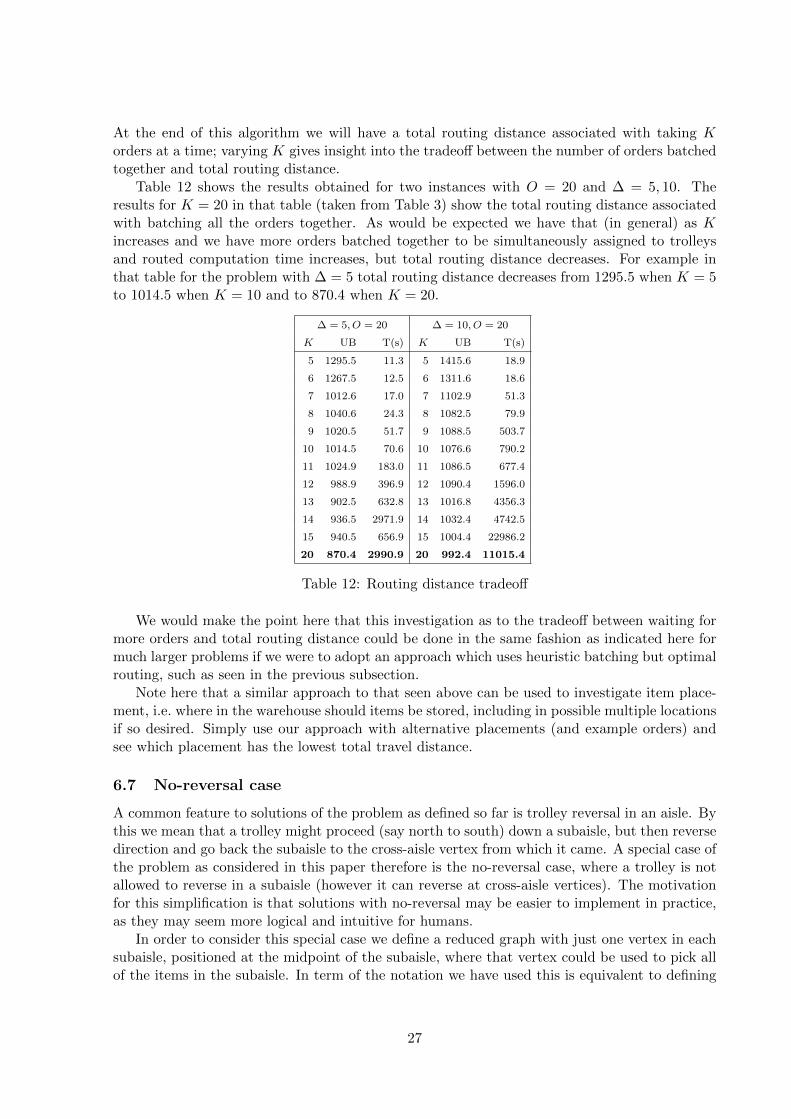
At the end of this algorithm we will have a total routing distance associated with taking Korders at a time; varying K gives insight into the tradeoff between the number of orders batchedtogether and total routing distance.

Table 12 shows the results obtained for two instances with O = 20 and ∆ = 5, 10. Theresults for K = 20 in that table (taken from Table 3) show the total routing distance associatedwith batching all the orders together. As would be expected we have that (in general) as Kincreases and we have more orders batched together to be simultaneously assigned to trolleysand routed computation time increases, but total routing distance decreases. For example inthat table for the problem with ∆ = 5 total routing distance decreases from 1295.5 when K = 5to 1014.5 when K = 10 and to 870.4 when K = 20.

∆ = 5, O = 20 ∆ = 10, O = 20

K UB T(s) K UB T(s)

5 1295.5 11.3 5 1415.6 18.9

6 1267.5 12.5 6 1311.6 18.6

7 1012.6 17.0 7 1102.9 51.3

8 1040.6 24.3 8 1082.5 79.9

9 1020.5 51.7 9 1088.5 503.7

10 1014.5 70.6 10 1076.6 790.2

11 1024.9 183.0 11 1086.5 677.4

12 988.9 396.9 12 1090.4 1596.0

13 902.5 632.8 13 1016.8 4356.3

14 936.5 2971.9 14 1032.4 4742.5

15 940.5 656.9 15 1004.4 22986.2

20 870.4 2990.9 20 992.4 11015.4

Table 12: Routing distance tradeoff

We would make the point here that this investigation as to the tradeoff between waiting formore orders and total routing distance could be done in the same fashion as indicated here formuch larger problems if we were to adopt an approach which uses heuristic batching but optimalrouting, such as seen in the previous subsection.

Note here that a similar approach to that seen above can be used to investigate item place-ment, i.e. where in the warehouse should items be stored, including in possible multiple locationsif so desired. Simply use our approach with alternative placements (and example orders) andsee which placement has the lowest total travel distance.

6.7 No-reversal case

A common feature to solutions of the problem as defined so far is trolley reversal in an aisle. Bythis we mean that a trolley might proceed (say north to south) down a subaisle, but then reversedirection and go back the subaisle to the cross-aisle vertex from which it came. A special case ofthe problem as considered in this paper therefore is the no-reversal case, where a trolley is notallowed to reverse in a subaisle (however it can reverse at cross-aisle vertices). The motivationfor this simplification is that solutions with no-reversal may be easier to implement in practice,as they may seem more logical and intuitive for humans.

In order to consider this special case we define a reduced graph with just one vertex in eachsubaisle, positioned at the midpoint of the subaisle, where that vertex could be used to pick allof the items in the subaisle. In term of the notation we have used this is equivalent to defining

27

R(a, c) = 1 ∀a ∈ A,∀c ∈ C. In addition, since we now cannot reverse in a subaisle, we can set:

xt,v(a,c),S(a,c,1) = xt,S(a,c,1),v(a,c+1) ∀a ∈ A, c ∈ C \ [WC ] (43)

xt,v(a,c+1),S(a,c,1) = xt,S(a,c,1),v(a,c) ∀a ∈ A, c ∈ C \ [WC ] (44)

These constraints ensure that if we use an arc to the vertex in the subaisle then we proceedonward to the next cross-aisle.

Clearly it might well be possible to produce a particularised formulation (e.g. based upon arcrouting) for this no-reversal case. However, since this special no-reversal case is not the primaryfocus of this paper, we have not explored this possibility.

Computational results given in Table 13 indicate how our approach performs when adapted(as indicated above) for the no-reversal case. Here, the results for the reinforced model withreversal are as in Table 3, but are repeated for convenience of comparison.

Two aspects are of interest in this case: performance improvements and how much larger aresolution values for the no-reversal case when compared to the reversal case. For analysing theseaspects we have added two extra columns to Table 13: T(s) ratio, defined as 100[no-reversalT(s)]/[reversal T(s)], shows how faster the no-reversal case is solved when compared to thereversal case. The UB ratio is defined as 100[no-reversal UB]/[reversal UB] - 100, which givesthe percentage increase in solution value for the no-reversal model compared to the reversalmodel. Only instances solved to optimality are assigned values in these columns, the averageratios also take into account these instances only.

For instances solved to optimality, solving the no-reversal case is considerably faster thansolving the reversal case, the time required for the former being on average only 12.6% of the timerequired for the latter. Additionally, the optimal solutions of the model without reversal are onaverage only 7.5% longer than the corresponding optimal solutions for the model with reversal.Rarely are optimal solutions without reversals more than 12% worse than corresponding optimalsolutions with reversals. The GAP and FGAP values also drop considerably for the no-reversalcase.

The improvement was however still not enough to prove optimality of the largest instances.However, the special case of no-reversal may be worthy of further investigation since optimalsolutions may be good enough for real-life problems, both in terms of distance travelled as wellas being more intuitive and easier to operate.

7 Application

Clearly in this paper we have adopted one particular type of order picking (where a trolley ispushed by a worker around aisles to collect the items needed for the orders assigned to thetrolley). Our consideration of this problem was motivated by discussions with a major UKsupermarket involved with home delivery of groceries. In other industries/contexts differentpicking methods (e.g. zone picking, bucket brigade picking) exist. However we believe that animportant application of the approach given in this paper is to supermarket home deliveries, asdiscussed further below.

Picking in the manner considered in this paper is widely used by supermarkets involved inhome delivery (e.g. see [Hays et al., 2005]). Indeed readers of this paper might themselves haveseen supermarket staff pushing trolleys around stores and picking items destined for home de-livery. The nature and economics of home delivery, where picking locations need to be relativelyclose to customers and where the capital investment associated with larger automated facilitiescan only be justified in areas of high population density, mean that human pickers with trolleys(based either in publicly accessible or dark stores) will continue to be a large proportion of such

28

∆ OReinforced model Reinforced model with the special case of no-reversal Ratios (%)

T(s) UB GAP LB FGAP FLB NS T(s) UB GAP LB FGAP FLB NS T(s) UB

5 5 3.9 348.6 – – 0.6 346.5 36 0.5 384.6 – – 2.1 376.5 77 12.8 10.3

6 2.9 364.8 – – 0.0 364.8 1 0.4 384.6 – – 0.0 384.6 1 13.8 5.4

7 8.9 374.8 – – 0.5 372.8 141 0.9 384.6 – – 0.2 383.8 3 10.1 2.6

8 95.2 503.8 – – 8.3 462.1 146 10.9 543.7 – – 5.3 515.0 27 11.4 7.9

9 151.8 539.6 – – 11.2 479.2 268 25.5 603.2 – – 9.4 546.8 397 16.8 11.8

10 111.0 581.4 – – 14.4 497.8 88 21.1 611.4 – – 6.3 572.9 101 19.0 5.2

11 97.1 613.5 – – 16.9 509.9 1009 16.8 641.7 – – 10.8 572.4 93 17.3 4.6

12 256.7 621.4 – – 15.0 527.9 2261 6.8 641.7 – – 9.6 579.9 85 2.6 3.3

13 168.9 623.4 – – 15.3 528.2 395 10.0 649.3 – – 9.2 589.3 114 5.9 4.2

14 263.8 639.3 – – 17.8 525.5 995 66.0 691.7 – – 14.9 588.5 1221 25.0 8.2

15 348.9 653.4 – – 20.0 522.4 975 27.3 699.8 – – 15.6 590.4 1710 7.8 7.1

20 2990.9 870.4 – – 31.2 598.4 28931 303.1 946.9 – – 26.4 696.6 20694 10.1 8.8

25 – 1127.4 17.8 927.0 43.2 640.8 123900 – 1155.1 5.8 1088.6 34.2 760.1 327653 – –

30 – 1221.9 26.8 894.3 47.0 647.5 70400 – 1295.0 16.4 1082.5 39.3 786.4 358800 – –

Avg 3407.1 3.2 17.2 16396.1 3120.7 1.6 13.1 50784.0 12.7 6.6

10 5 1.5 371.1 – – 0.0 371.1 1 0.1 384.6 – – 0.0 384.6 1 6.7 3.6

6 6.6 377.1 – – 0.6 374.7 207 0.4 384.6 – – 0.0 384.6 1 6.1 2.0

7 197.5 549.8 – – 8.4 503.4 13 16.2 613.1 – – 4.5 585.8 124 8.2 11.5

8 286.8 584.2 – – 13.0 508.4 110 22.0 681.2 – – 9.2 618.7 1497 7.7 16.6

9 356.1 637.4 – – 17.1 528.6 8608 17.1 681.2 – – 9.3 618.1 201 4.8 6.9

10 393.0 661.8 – – 16.4 553.4 10439 24.6 729.3 – – 9.3 661.7 3126 6.3 10.2

11 383.7 699.8 – – 20.9 553.8 21044 17.2 729.7 – – 10.1 656.1 348 4.5 4.3

12 217.7 707.7 – – 21.8 553.6 2481 21.2 731.3 – – 9.1 664.7 515 9.7 3.3

13 385.4 725.7 – – 22.8 560.2 10370 98.5 769.2 – – 13.1 668.7 6038 25.6 6.0

14 483.8 727.8 – – 22.7 562.4 8597 102.2 769.2 – – 14.8 655.7 6755 21.1 5.7

15 1832.6 882.6 – – 32.8 593.1 26398 176.4 930.0 – – 23.9 707.3 12528 9.6 5.4

20 11015.4 992.4 – – 32.3 672.0 70496 172.2 1028.3 – – 21.5 807.5 15586 1.6 3.6

25 – 1213.4 16.7 1011.3 41.7 707.8 133600 – 1264.7 5.8 1190.7 32.8 849.5 276700 – –

30 – 1330.0 27.6 963.1 46.9 706.3 74100 – 1400.5 18.4 1142.8 40.2 836.9 318200 – –

Avg 4197.2 3.2 21.2 26176.0 3133.4 1.7 14.1 45830.0 9.3 6.6

20 5 110.9 573.8 – – 6.7 535.3 233 8.5 623.3 – – 0.0 623.3 1 7.7 8.6

6 278.9 656.2 – – 11.5 580.9 1164 11.6 729.3 – – 6.9 679.3 734 4.2 11.1

7 263.2 689.8 – – 17.2 571.4 579 24.9 769.2 – – 9.2 698.1 3678 9.5 11.5

8 189.0 697.8 – – 18.5 568.7 2886 18.3 769.2 – – 11.6 679.9 2795 9.7 10.2

9 305.5 727.7 – – 20.6 578.0 3620 49.4 769.2 – – 10.4 689.3 1293 16.2 5.7

10 584.2 920.5 – – 31.1 634.2 7198 115.9 990.0 – – 20.1 790.8 3435 19.8 7.6

11 703.8 980.5 – – 31.4 672.9 10620 132.4 1075.8 – – 22.4 834.6 8361 18.8 9.7

12 830.1 1004.3 – – 33.7 666.0 20221 241.6 1113.8 – – 23.9 847.9 29783 29.1 10.9

13 1177.8 1009.1 – – 31.0 696.5 30072 187.3 1113.8 – – 23.5 851.7 28029 15.9 10.4

14 1306.0 1011.1 – – 32.8 679.2 8097 467.5 1113.9 – – 28.4 797.6 23297 35.8 10.2

15 3793.7 1028.7 – – 34.7 671.5 38243 348.7 1115.9 – – 28.4 798.7 24610 9.2 8.5

20 – 1335.2 15.8 1124.6 45.4 729.0 67600 – 1453.0 5.9 1367.0 37.4 910.0 341800 – –

25 – 1694.9 31.2 1166.8 51.4 824.5 67200 – 1769.5 17.1 1466.5 40.2 1058.4 387359 – –

30 – 1966.9 45.5 1071.9 56.6 853.4 33400 – 2041.8 29.5 1440.3 47.0 1082.6 360245 – –

Avg 5310.2 6.6 30.2 20795.2 4743.3 3.8 22.1 86815.7 16.0 9.5

Avg all 4304.8 4.3 22.9 21122.5 3665.8 2.4 16.4 61143.2 12.6 7.5

Table 13: Comparison of the reinforced model with and without the no-reversal special case.IBC was used in both cases.

29

operations, both for supermarkets in the UK and world-wide. This is especially true for super-markets with a national presence (such as many in the UK) whose home delivery operationsoperate nationwide.

With regard to the advantages of applying optimisation [Bartholdi and Hackman, 2016] state:“warehouses that are most likely to benefit from pick-path optimization are those that have manyitems, most of which are slow-moving, and customer orders of moderate size”. Orders fromcustomers to supermarkets for home delivery fall into this category. Moreover the supermarketbusiness is a relatively low profit margin business and so pressure always exists to reduce costsappropriately. Obviously the use of optimisation to more effectively utilise pickers can aid inmaking home delivery operations more cost efficient.

Clearly the difficulties in applying optimisation in the supermarket situation relate to com-municating to the human trolley operator the precise route to be followed and ensuring thatthe route given is not overly complex. Overcoming these difficulties relies on a combination oftechnology and appropriate routing. In terms of technology a simple handheld device (such asalready used by supermarket pickers in order to know which items to pick) can be easily adaptedto display instructions such as “now go to the end of aisle, turn left and back up the next aisle”.In terms of appropriate routing note that above we considered the no-reversal case, in which atrolley is not allowed to reverse in a subaisle. Our belief is that routes of this kind are simplyeasier for pickers to understand and follow as compared to routes which demand reversal in asubaisle.

With regard to the specific order characteristics used in this paper we applied our bestjudgement to enable us to produce orders with characteristics as close to online grocery ordersas achievable within the constraint of using a publicly available dataset (Foodmart). Using sucha dataset means that we are able to make all the instances used in this paper publicly availablefor use by future workers.

8 Conclusions and future work

In this work we investigated the joint order batching and picker routing problem in storage areas.According to our literature review, very few exact methods have been proposed by any otherauthors, none for the case of warehouses composed of multiple blocks. We introduced a formu-lation and a significant number of valid inequalities (cuts) for the problem. Our results showedgreatly improved performance. In fact, many potentially disconnected solutions are naturallyprevented due to the addition of these new cuts. Instances involving up to 20 orders were solvedto proven optimality when we jointly considered order batching and picker routing. Instancesinvolving up to 5000 orders were considered where order batching was done heuristically, butpicker routing done optimally.

In future we plan to study new algorithms for both JOBPRP and the special case of no-reversal, introduced in Section 6.7. We believe that column generation based methods, suchas branch-and-price or branch-and-cut-and-price (BCP), may be viable alternatives. Fukasawaet al. [2006] and Baldacci et al. [2008] developed successful BCPs for the closely related Ca-pacitated VRP and Letchford and Oukil [2009] proposed column generation methods that ex-ploit sparsity for the also closely related Capacitated Arc Routing Problem (CARP). If non-elementary routes are allowed (routes where edges/vertices may be revisited), then the authorsshowed that exact pricing can be computed polynomially. In our opinion, a BCP approach forthe JOBPRP should exploit its sparse nature and perhaps an effective pricing algorithm canalso be obtained. Moreover, we also believe that a CARP based formulation may be beneficialfor the special case of no-reversal, in which a similar method to that in [Letchford and Oukil,

30

2009] may be achievable.We also plan to conduct a theoretical study of the strength of each valid inequality and to

potentially characterize new valid inequalities that could be added to further reinforce linearrelaxation bounds. Finally, we intend to study assignment heuristics where optimal routingreplaces (at least partially) approximate route estimates.

References

M. Albareda-Sambola, A. Alonso-Ayuso, E. Molina, and C. S. de Blas. Variable neighbor-hood search for order batching in a warehouse. Asia-Pacific Journal of Operational Research(APJOR), 26(05):655–683, 2009. doi: 10.1142/S0217595909002390.

A. H. Azadnia, S. Taheri, P. Ghadimi, M. Z. M. Saman, and K. Y. Wong. Order batchingin warehouses by minimizing total tardiness: a hybrid approach of weighted association rulemining and genetic algorithms. The Scientific World Journal, 2013(1):1–13, 2013. doi: 10.1155/2013/246578.

R. Baldacci, N. Christofides, and A. Mingozzi. An exact algorithm for the vehicle routingproblem based on the set partitioning formulation with additional cuts. Mathematical Pro-gramming, 115(2):351–385, 2008. doi: 10.1007/s10107-007-0178-5.

J. J. Bartholdi and S. T. Hackman. Warehouse & Distribution Science, Release 0.97. Availablefrom http://www2.isye.gatech.edu/∼jjb/wh/book/index.html, 2016.

J. M. Belenguer and E. Benavent. The capacitated arc routing problem: valid inequalities andfacets. Computational Optimization and Applications, 10(2):165–187, 1998. doi: 10.1023/A:1018316919294.

A. Bosco, D. Lagana, R. Musmanno, and F. Vocaturo. Modeling and solving the mixedcapacitated general routing problem. Optimization Letters, 7(7):1451–1469, 2013. doi:10.1007/s11590-012-0552-y.

M. C. Chen and H. P. Wu. An association-based clustering approach to order batching consid-ering customer demand patterns. Omega, 33(4):333–343, 2004. doi: 10.1016/j.omega.2004.05.003.

G. Cornuejols, D. Naddef, and W. R. Pulleyblank. Halin graphs and the travelling salesmanproblem. Mathematical Programming, 26(3):287–294, 1983. doi: 10.1007/BF02591867.

G. Cornuejols, J. Fonlupt, and D. Naddef. The travelling salesman problem on a graph andsome related integer polyhedra. Mathematical Programming, 33(1):1–27, 1985. doi: 10.1007/BF01582008.

CPLEX Optimizer. IBM. Available from http://www-01.ibm.com/software/integration/optimization/cplex-optimizer/, last accessed June 15th 2016, 2016.

R. de Koster, E. S. van der Poort, and M. Wolters. Efficient order batching methods inwarehouses. International Journal of Production Research, 37(7):1479–1504, 1999. doi:10.1080/002075499191094.

R. De Koster, T. Le-Duc, and K. J. Roodbergen. Design and control of warehouse order picking:a literature review. European Journal of Operational Research, 182(2):481–501, 2007. doi:10.1016/j.ejor.2006.07.009.

31

R. Dekker, M. B. M. de Koster, K. J. Roodbergen, and H. van Kalleveen. Improving order-picking response time at Ankor’s warehouse. Interfaces, 34(4):303–313, 2004. doi: 10.1287/inte.1040.0083.

B. Fleischmann. A cutting-plane procedure for the traveling salesman problem on a roadnetwork. European Journal of Operational Research, 21(3):307–317, 1985. doi: 10.1016/0377-2217(85)90151-1.

J. Fonlupt and A. Nachef. Dynamic programming and the graphical traveling salesman problem.Journal of the ACM, 40(5):1165–1187, 1993. doi: 10.1145/174147.169803.

J. Fonlupt and D. Naddef. The travelling salesman problem in graphs with some excludedminors. Mathematical Programming, 53(2):147–172, 1992. doi: 10.1007/BF01585700.

R. Fukasawa, H. Longo, J. Lysgaard, M. P. Aragao, M. Reis, E. Uchoa, and R. F. Werneck.Robust branch-and-cut-and-price for the capacitated vehicle routing problem. MathematicalProgramming, 106(3):491–511, 2006. doi: 10.1007/s10107-005-0644-x.

D. R. Gibson and G. P. Sharp. Order batching procedures. European Journal of OperationalResearch, 58(1):57–67, 1992. doi: 10.1016/0377-2217(92)90235-2.

A. V. Goldberg and R. E. Tarjan. A new approach to the maximum flow problem. Journal ofthe ACM, 35(4):921–940, 1988. doi: 10.1145/48014.61051.

P. Hart, N. Nilsson, and B. Raphael. A formal basis for the heuristic determination of minimumcost paths. IEEE Transactions on Systems Science and Cybernetics, 4(2):100–107, 1968. doi:10.1145/1056777.1056779.

T. Hays, P. Keskinocak, and V. M. de Lopez. Strategies and challenges of internet groceryretailing logistics, pages 217–252. Kluwer Academic Publishers, 2005.

S. Henn and V. Schmid. Metaheuristics for order batching and sequencing in manual orderpicking systems. Computers & Industrial Engineering, 66(2):338–351, 2013. doi: 10.1016/j.cie.2013.07.003.

S. Henn and G. Wascher. Tabu search heuristics for the order batching problem in manualorder picking systems. European Journal of Operational Research, 222(3):484–494, 2012. doi:10.1016/j.ejor.2012.05.049.

S. Henn, S. Koch, and G. Wascher. Order batching in order picking warehouses: a surveyof solution approaches, chapter 6, pages 105–137. Springer London, 2012. doi: 10.1007/978-1-4471-2274-6 6.

S. Hong, A. L. Johnson, and B. A. Peters. Batch picking in narrow-aisle order picking systemswith consideration for picker blocking. European Journal of Operational Research, 221(3):557–570, 2012a. doi: 10.1016/j.ejor.2012.03.045.

S. Hong, A. L. Johnson, and B. A. Peters. Large-scale order batching in parallel-aisle pickingsystems. IIE Transactions, 44(2):88–106, 2012b. doi: 10.1080/0740817X.2011.588994.

S. Hong, A. L. Johnson, and B. A. Peters. Order batching in a bucket brigade order pickingsystem considering picker blocking. Flexible Services and Manufacturing Journal, 28(3):425–441, 2016. doi: 10.1007/s10696-015-9223-5.

32

J. N. Hooker, H. Yan, I.E. Grossmann, and R. Raman. Logic cuts for processing networks withfixed charges. Computers & Operations Research, 21(3):265–279, 1994. doi: http://dx.doi.org/10.1016/0305-0548(94)90089-2.

C. M. Hsu, K. Y. Chen, and M. C. Chen. Batching orders in warehouses by minimizing traveldistance with genetic algorithms. Computers in Industry, 56(2):169–178, 2004. doi: 10.1016/j.compind.2004.06.001.

Stefan Irnich, Demetrio Lagan, Claudia Schlebusch, and Francesca Vocaturo. Two-phase branch-and-cut for the mixed capacitated general routing problem. European Journal of OperationalResearch, 243(1):17–29, 2015. doi: http://dx.doi.org/10.1016/j.ejor.2014.11.005.

C. H.Y. Lam, K.L. Choy, G.T.S. Ho, and C.K.M. Lee. An order-picking operations system formanaging the batching activities in a warehouse. International Journal of Systems Science,45(6):1283–1295, 2014. doi: 10.1080/00207721.2012.761461.

A. N. Letchford and A. Oukil. Vehicle routing on sparse graphs: a literature review and ananalysis. Unpublished manuscript, 2006.

A. N. Letchford and A. Oukil. Exploiting sparsity in pricing routines for the capacitated arcrouting problem. Computers & Operations Research, 36(7):2320–2327, 2009. doi: 10.1016/j.cor.2008.09.008.

A. N. Letchford, S. D. Nasiri, and D. O. Theis. Compact formulations of the Steiner travelingsalesman problem and related problems. European Journal of Operational Research, 228(1):83–92, 2013. doi: 10.1016/j.ejor.2013.01.044.

S. Lin and B. W. Kernighan. An effective heuristic algorithm for the traveling-salesman problem.Operations Research, 21(2):498–516, 1973. doi: 10.1287/opre.21.2.498.

A. Lucena. Steiner problem in graphs: lagrangean relaxation and cutting planes. COAL Bulletin,21(1):2–8, 1992.

M. Matusiak, R. de Koster, L. Kroon, and J. Saarinen. A fast simulated annealing methodfor batching precedence-constrained customer orders in a warehouse. European Journal ofOperational Research, 236(3):968–977, 2014. doi: 10.1016/j.ejor.2013.06.001.

MySQL Foodmart Database. Available from http://pentaho.dlpage.phi-integration.com/mondrian/mysql-foodmart-database (last accessed June 15th 2016), 2008.

D. Naddef. Polyhedral theory and branch-and-cut algorithms for the symmetric TSP, pages29–116. Springer US, 2007. doi: 10.1007/0-306-48213-4 2.

C. S. Orloff. A fundamental problem in vehicle routing. Networks, 4(1):35–64, 1974. doi:10.1002/net.3230040105.

M. Padberg and G. Rinaldi. Optimization of a 532-city symmetric traveling salesman problemby branch-and-cut. Operations Research Letters, 6(1):1–7, 1987. doi: 10.1137/1033004.

M. Padberg and G. Rinaldi. A branch-and-cut algorithm for the resolution of large-scale sym-metric traveling salesman problems. SIAM Review, 33(1):60–100, 1991. doi: 10.1137/1033004.

C. G. Petersen II. An evaluation of order picking routing policies. International Jour-nal of Operations & Production Management, 17(11):1098–1111, 1997. doi: 10.1080/00207540410001696339.

33

H. D. Ratliff and A. S. Rosenthal. Order-picking in a rectangular warehouse: a solvable caseof the traveling salesman problem. Operations Research, 31(3):507–521, 1983. doi: 10.1287/opre.31.3.507.

K. J. Roodbergen and R. de Koster. Routing methods for warehouses with multiple crossaisles. International Journal of Production Research, 39(9):1865–1883, 2001a. doi: 10.1080/00207540110028128.

K. J. Roodbergen and R. de Koster. Routing order pickers in a warehouse with a middle aisle.European Journal of Operational Research, 133(1):32–43, 2001b. doi: 10.1016/S0377-2217(00)00177-6.

A. Schloz, S. Henn, M. Stuhlmann, and G. Wascher. A new mathematical programming formu-lation for the single-picker routing problem. European Journal of Operational Research, 253(1):68–84, 2016. doi: 10.1016/j.ejor.2016.02.018.

C. Theys, O. Braysy, W. Dullaert, and B. Raa. Using a TSP heuristic for routing order pickersin warehouses. European Journal of Operational Research, 200(3):755–763, 2010. doi: 10.1016/j.ejor.2009.01.036.

J. A. Tompkins, J.A. White, Y.A. Bozer, and J.M.A. Tanchoco. Facilities Planning, 4th Edition.John Wiley & Sons, 2010.

C. A. Valle, J. E. Beasley, and A. S. Cunha. Modelling and solving the joint order batching andpicker routing problem in inventories, pages 81–97. LNCS. Springer International Publishing,2016. doi: 10.1007/978-3-319-45587-7 8.

34