Tabu Search Heuristics for the Order Batching Problem in ...

Tabu Search Heuristics for the Order Batching Problem in Manual Order Picking Systems

Sebastian Henn � Gerhard Wäscher

FEMM Working Paper No. 07, February 2010

OTTO-VON-GUERICKE-UNIVERSITY MAGDEBURG

FACULTY OF ECONOMICS AND MANAGEMENT

F E M M Faculty of Economics and Management Magdeburg

Working Paper Series

Otto-von-Guericke-University Magdeburg

Faculty of Economics and Management

P.O. Box 4120

39016 Magdeburg, Germany

http://www.ww.uni-magdeburg.de/

http://www.ww.uni-magdeburg.de/

Impressum (§ 5 TGM):

Herausgeber: Otto-von-Guericke-Universität Magdeburg Fakultät für Wirtschaftswissenschaft Die Dekanin

Verantwortlich für diese Ausgabe: Gerhard Wäscher Otto-von-Guericke-Universität Magdeburg Postfach 4120 39016 Magdeburg

http://www.ww.uni-magdeburg.de/fwwdeka/femm/

Auflage: (50)

Redaktionsschluss: Februar 2010

Herstellung: Dezernat Allgemeine Angelegenheiten, Sachgebiet Reproduktion

Bezug über den Herausgeber

ISSN 1615-4274

Tabu Search Heuristics for the Order Batching

Problem in Manual Order Picking Systems

Sebastian Henn, Gerhard Wascher

February 2010

Abstract

In manual order picking systems, order pickers walk or ride through a distribution ware-

house in order to collect items requested by (internal or external) customers. In order to

perform these operations efficiently, it is usually required that customer orders are combined

into (more substantial) picking orders of limited size. The Order Batching Problem consid-

ered in this paper deals with the question of how a given set of customer orders should be

combined such that the total length of all tours necessary to collect all items is minimized.

For the solution of this problem the authors suggest two approaches based on the tabu

search principle. The first one is a straightforward classic Tabu Search algorithm (TS), the

second one is the Attribute-Based Hill Climber (ABHC). In a series of extensive numerical

experiments, the newly developed approaches are benchmarked against different solution

methods from literature. It is demonstrated that the proposed methods are superior to ex-

isting methods and provide solutions which may allow for operating distribution warehouses

significantly more efficiently.

Keywords: Logistics, Warehouse Management, Order Batching, Tabu Search, Attribute-Based

Hill Climber

Corresponding author:

Dipl.-Math. oec. Sebastian Henn

Otto-von-Guericke-University Magdeburg

Faculty of Economics and Management

Department of Management Science

Postbox 4120

39106 Magdeburg

[email protected]

Contents

1 Introduction 1

2 Order Batching Problem 2

2.1 Problem Description . . . . . . . . . . . . . . . . . . . . . . . . . . . . . . . . . . 2

2.2 Model Formulation . . . . . . . . . . . . . . . . . . . . . . . . . . . . . . . . . . . 3

3 Literature Review 4

4 Tabu Search 5

4.1 General Principle . . . . . . . . . . . . . . . . . . . . . . . . . . . . . . . . . . . . 5

4.2 Specifications for the OBP . . . . . . . . . . . . . . . . . . . . . . . . . . . . . . . 6

5 Attribute-Based Hill Climber 7

5.1 General Principle . . . . . . . . . . . . . . . . . . . . . . . . . . . . . . . . . . . . 7

5.2 Specifications for the OBP . . . . . . . . . . . . . . . . . . . . . . . . . . . . . . . 8

6 Design of the Computational Experiments 9

6.1 Warehouse Parameters . . . . . . . . . . . . . . . . . . . . . . . . . . . . . . . . . 9

6.2 Problem Classes . . . . . . . . . . . . . . . . . . . . . . . . . . . . . . . . . . . . . 10

6.3 Upper Bound . . . . . . . . . . . . . . . . . . . . . . . . . . . . . . . . . . . . . . 10

6.4 Implementation and Hardware . . . . . . . . . . . . . . . . . . . . . . . . . . . . . 10

7 Configuration Pretests for TS 11

7.1 S-Shape-Routing . . . . . . . . . . . . . . . . . . . . . . . . . . . . . . . . . . . . 11

7.2 Largest Gap-Routing . . . . . . . . . . . . . . . . . . . . . . . . . . . . . . . . . . 12

8 Configuration Pretests for ABHC 13

8.1 S-Shape-Routing . . . . . . . . . . . . . . . . . . . . . . . . . . . . . . . . . . . . 13


9 Comparative Tests 14

9.1 Benchmarks . . . . . . . . . . . . . . . . . . . . . . . . . . . . . . . . . . . . . . . 14

9.2 S-Shape-Routing . . . . . . . . . . . . . . . . . . . . . . . . . . . . . . . . . . . . 15


10 Conclusions and Outlook 19

Sebastian Henn, Gerhard Wascher 1

1 Introduction

Order picking is a warehouse function dealing with the retrieval of articles (items) from their stor-

age location in order to satisfy a given demand specified by (internal or external) customer orders

(Petersen and Schmenner, 1999). Order picking arises because incoming articles are received and

stored in (large-volume) unit loads while customers order small volumes (less-than-unit loads) of

different articles. On the one hand, underperformance in order picking may result in an unsatis-

factory customer service (long processing and delivery times, incorrect shipments); on the other,

it may lead to high costs (labor cost, cost of additional and/or emergency shipments), since more

than 50% of the total operative costs of a warehouse are related to order picking (Frazelle, 2002).

Both aspects may have a negative impact on the competitiveness of the warehouse.

Like many other repetitive material-handling activities, order picking is still a function which

involves the employment of human operators at a large scale. Even though various attempts have

been made to automate the picking process, manual order picking systems are still prevalent in

practice. Such systems can be differentiated into two categories: picker-to-parts systems, in which

order pickers walk or ride through the warehouse and collect the requested items, and parts-to-

picker systems, in which automated storage and retrieval systems deliver the items to stationary

order pickers (Wascher, 2004). With respect to systems of the first kind, three planning problems

can be distinguished on the operative level (Caron et al., 1998): the assignment of articles to

storage locations (article location), the grouping of customer orders into picking orders (order

batching), and the routing of order pickers through the warehouse (picker routing).

This paper deals with the second activity, which has proven to be pivotal for the efficiency of

warehouse operations (de Koster et al., 1999).

Henn et al. (2009) have shown that the application of a local search-based metaheuristic, namely

Iterated Local Search, to the Order Batching Problem can improve the warehouse efficiency

substantially. In their experiments, however, the application of the proposed algorithm turned

out to be very time-consuming, and, in particular, not suitable for picking environments where

solutions have to be generated quickly or even in real time. This article focuses on two other

types of local search-based approaches, which have demonstrated to provide high-quality solutions

within marginal computing times for related combinatorial optimization problems. The first one

is a straightforward application of Tabu Search (TS); the second one is the Attribute-Based Hill

Climber (ABHC), which is also based on a tabu search principle, but does only require to specify

a small number of parameters.

The remainder of the paper is organized as follows: In Section 2 the Order Batching Problem

(OBP) will be defined. Section 3 contains a literature review of solution approaches for the OBP.

In the subsequent section the straightforward TS implementation is described. In Section 5 it

is shown how the general principle of ABHC can be applied to the OBP. Extensive numerical

experiments have been carried out in order to evaluate the performance of the metaheuristics.

Section 6 is dedicated to the design of these experiments (including the description of warehouse

parameters, algorithm parameters, and problem classes). The performance of TS and ABHC

is analyzed for different configurations in Section 7 and Section 8, respectively. A comparative

2 Tabu Search Heuristics for the Order Batching Problem in Manual Order Picking Systems

analysis of the proposed method against benchmark heuristics and optimal solutions is presented

in Section 9. The article concludes with a summary on the main contributions of the work and

an outlook on further research opportunities.

2 Order Batching Problem

2.1 Problem Description

A customer order consists of a (non-empty) set of order lines, where each order line consists of a

particular article and the corresponding requested quantity. A pick list contains the order lines

which should be processed together and guides the order picker through the warehouse. This

list may contain the order lines of a single customer order (pick-by-order) or of a combination of

customer orders (pick-by-batch). In practice, the sequence in which the items are to be picked

and the corresponding route of the order picker (who starts at the depot, proceeds to the respec-

tive storage locations, and returns to the depot) are usually determined by means of a so-called

routing strategy. Since order pickers seem to accept only straightforward and non-confusing rout-

ing schemes, routes provided by the S-Shape- or Largest Gap-Heuristics are prevalent in practice

(de Koster et al., 1999). The character of these heuristics is exemplified in Figure 2.1. The black

rectangles symbolize the locations of items to be picked on the respective routes.

Solutions provided by the S-Shape-Heuristic are characterized as follows: the order picker enters

an aisle if at least one requested item is located in that aisle and traverses the aisle completely.

Afterwards, the order picker proceeds to the next aisle which contains a requested item. An

exception could be the last aisle: if the order picker is positioned in the front cross-aisle, he/she

would pick the items of the last aisle and return to the depot along the front aisle. The Largest

Gap-Heuristic gives a solution in which the order picker entirely traverses the rightmost and left-

most aisle containing an item to be picked. All the other aisles are entered from the front and

back aisle in such a way that the non-traversed distance between two adjacent locations of items

to be picked in the aisle is maximal.

Figure 2.1: Example of S-Shape (left) and Largest Gap (right) in a single-block warehouse


For the collection of the requested items, order pickers are usually taking advantage of a picking

device (e.g. a cart or a roll pallet). Customer orders can be combined into picking orders until

the capacity of the device is exhausted. Splitting of customer orders is usually not permitted

since it would result in an additional, not acceptable sorting effort.

With respect to the availability of information of customer orders, order batching can be distin-

guished into off-line batching and on-line batching (Yu and de Koster, 2009). The off-line case,

which is covered in this paper, considers an order picking environment where all customer orders

are known in advance. In the on-line case customer orders arrive at different points in time.

Due to the high amount of time-consuming manual operations, the minimization of picking times

is of great importance for controlling the picking process efficiently. The time spent by order

pickers to collect the items of all customer orders (total picking time) consist of the setup times

for the routes, the travel times that are needed to travel to, from, and between the locations

of items to be picked, the search times for the identification of the items, and the times needed

for picking the items. Among these components, the travel time is of outstanding importance,

since it consumes the major proportion of the total order picking time (at least 50% of the order

picker’s time), while the other components can either be assumed as constant (search times and

pick times) or as neglectable (setup times) (Tompkins et al., 2003). Furthermore, given that the

pickers’ travel velocity is constant, the minimization of the total travel time is equivalent to the

miminization of the total length of all picker tours (Jarvis and McDowell, 1991).

The Order Batching Problem can then be summarized and defined as follows: How can a given

set of customer orders, with given storage locations, given routing strategy and given capacity

of the picking devices, be grouped (batched) into picking orders such that the total length of all

necessary picking tours (total tour length) is minimized (Wascher, 2004).

2.2 Model Formulation

According to Gademann and van de Velde (2005), a mathematical formulation of the problem

can be given as follows: Let J = {1, . . . , n} be the set of customer orders, C the capacity of the

picking device, and cj the capacity required for order j (j ∈ J). Furthermore, let each batch of

customer orders be described by a vector ai = (ai1, ..., ain) with binary entries aij stating whether

an order j is included in a batch i (aij = 1) or not (aij = 0). The set I of all feasible batches is

characterized by the fact that the capacity of the picking device is not violated, i.e. the following

property holds:

∑

j∈J

cj · aij ≤ C, ∀i ∈ I. (2.1)

Let xi (i ∈ I) be a binary decision variable, which describes if a batch i is chosen (xi = 1) or not

(xi = 0), and let di further represent the length of the picking tour in which all orders of a batch


i are collected, then the following optimization model can be formulated for the OBP:

min∑

i∈I

di · xi (2.2)

s.t.∑

i∈I

aij · xi = 1, ∀j ∈ J ; (2.3)

xi ∈ {0, 1}, ∀i ∈ I. (2.4)

The sets of constraints (2.3) and (2.4) ensure that a set of batches is chosen in a way that each

customer order is included in exactly one of the chosen batches. The number of possible batches

and, therefore, the number of binary variables grows exponentially with the number of orders.

The OBP as described above is known to be NP-hard (in the strong sense) if the number of

orders per batch is greater than two (Gademann and van de Velde, 2005).

3 Literature Review

So far, only few approaches have been described in the literature which solve the OBP to or

close to optimality. Gademann and van de Velde (2005) describe a mixed integer programming

model and a branch-and-price algorithm with column generation that was able to provide optimal

solutions for small instances (up to 32 orders). For the case of S-Shape-Routing Bozer and Kile

(2008) present a mixed integer programming approach that generates near optimal solutions for

small (up to 25) order sizes.

For larger problems – as they usually occur in practice – the use of heuristics is essential. Heuris-

tics for the OBP can be distinguished into four groups: priority rule-based algorithms, seed

algorithms, savings algorithms, and metaheuristics. The first three groups contain approaches

of the constructive type (Wascher, 2004), whereas metaheuristic approaches are mainly of an

improvement type.

In priority rule-based algorithms the customer orders are first ranked according to a priority value

and then assigned to batches following this ranking (Gibson and Sharp, 1992). The probably best

known and most straightforward way consists of the application of the First-Come-First-Served

rule (FCFS). Other priority rules include space-filling curves (Gibson and Sharp, 1992; Pan and

Liu, 1995). The assignment of customer orders to batches can either be done sequentially (Next-

Fit-Rule) or simultaneously (First-Fit-Rule, Best-Fit-Rule) (Wascher, 2004).

The second group, introduced by Elsayed (1981) and Elsayed and Stern (1983), is formed by seed

algorithms, which generate batches sequentially. They select one customer order as an initial

order for a batch. Additional customer orders are assigned to that batch according to an order-

congruency rule. An overview of the various seed selection and order-congruency rules is given

by de Koster et al. (1999), Ho and Tseng (2006) and Ho et al. (2008).

Savings algorithms are based on the Clarke-and-Wright-Algorithm for the Vehicle Routing Prob-

lem (Clarke and Wright, 1964) and have been adapted in several ways for the OBP. In its initial

version for the OBP (C&W(i)), for each combination of customer orders i and j the savings savij


are computed which can be obtained by collecting the items of the two customer orders on one

(large) tour instead of collecting them in two separate tours. Starting with the pair of orders with

the highest savings, the pairs are considered for being assigned to a batch in a non-ascending

order. This may lead to three situations: in case that none of the two orders has been assigned, a

new batch will be opened for them; if one of the orders has already been assigned, the other one

is added to the batch if the remaining capacity is sufficient; in case that not enough capacity is

available or that both orders have already been assigned, the next pair of orders will be consid-

ered. All orders left unallocated at the end of the process will be assigned to an individual batch

each. The algorithm can be improved by recalculating the savings each time orders have been

allocated to a batch (C&W(ii)) (Elsayed and Unal, 1989).

Comprehensive numerical experiments (de Koster et al., 1999) have shown that among the con-

structive heuristics either seed algorithms or savings algorithms provide the best solutions with

respect to the total tour length, dependent on the warehouse layout and on customer order char-

acteristics.

Finally, the last group of solution approaches to the OBP is formed by metaheuristics. Hsu et al.

(2005) have suggested a genetic algorithm for the OBP. Their approach includes an aisle-metric

for the determination of the tour lengths and is, therefore, limited to S-Shape-Routing, only.

Tsai et al. (2008) describe an integrated approach, in which both batching and routing problems

are solved by means of a genetic algorithm. Due to these specific conditions, both approaches

will not be considered here any further. Gademann and van de Velde (2005) propose an iterated

improvement algorithm that incorporates a 2-opt neighborhood. Henn et al. (2009) apply two

methods for solving the OBP, namely Iterated Local Search and a Rank-Based Ant System. By

means of numerical experiments the authors demonstrate that both approaches outperform the

constructive algorithms, yet at the expense of long computing times.

Finally, Chen and Wu (2005) describe an order batching approach based on data mining and

integer programming. In this approach, at first similarities of customer orders are determined

by means of an association rule; then a 0-1 integer programming approach is applied in order to

cluster the orders into batches.

4 Tabu Search

4.1 General Principle

In combinatorial optimization, a solution S has to be found in the set of all feasible solutions F

which has a minimal (or maximal) value for an objective function d. A minimization problem

can, therefore, be described as

min{d(S)|S ∈ F}. (4.1)

A simple and widely-used method to solve combinatorial optimization problems is local search

(LS): For a solution S (S ∈ F) the subset N (S) of F is called neighborhood of S in which each


solution S ′ ∈ N (S) can be obtained by applying a single local transformation (”move”) to S.

Local search generates a sequence of solutions S0, S1, S2, . . . , where each member of the sequence

is an element of the neighborhood of its predecessor. Each element possesses a smaller objective

function value than the previous one. The disadvantage of local search is that the sequence

terminates at a local optimum, which – for large problem sizes – does not necessarily represent a

global optimum, and the corresponding objective function value may differ significantly from to

the optimal one. Therefore, different approaches based on the LS principle have been designed

in order to overcome such local optima by allowing also deteriorations of the objective function

value during the search.

Tabu Search – as a specific local search-based method – was developed by Glover (1986) and

aims at simulating human memory processes. This memory process is implemented by a tabu list

which records moves applied in previous iterations. The application of these moves is forbidden

(”tabu”) for a particular number of iterations in order to avoid cycling and to diversify the search.

In each iteration Tabu Search considers only those elements of the neighborhood as new incumbent

solutions which can be obtained by a non-tabu move. After having accepted a new solution, the

tabu list is updated. The algorithm stops when a termination condition is met. Algorithm 4.1

summarizes the general principle of Tabu Search, to which a variety of extensions and features

can be added (Glover and Laguna, 1997).

Algorithm 4.1 Tabu Search: General Principle

Input: initial solution S0, tabu list T ;

S⋆ := S0;

repeat

generate N (Si);

delete solutions from N (Si) which were obtained by a tabu move;

5: select solution from N (Si) as next solution Si+1;

update T according to Si, Si+1 and i;

i := i + 1;

until termination condition is met;

4.2 Specifications for the OBP

For the generation of the initial solution we suggest two options, namely generation according to

the FCFS-rule (FCFS in this context means that costumer orders are assigned to batches accord-

ing to their index) and generation by application of C&W(ii). Whereas a solution (defined as a

set of batches) generated by FCFS is a totally random solution, solutions obtained by C&W(ii)

may already be identical to or close to local minima.

For the neighborhood structure of a solution S we consider three different options. The first

one, Nswap(S), is the set of solutions which can be obtained from S by interchanging two or-

ders from different batches (swap). The second one, Nshift(S), is the set of solutions which


can be generated by assigning one order to a different batch (shift). The third neighborhood

structure is defined by a combination of swaps and shifts, i.e. the set of solutions is given by

Ncom(S) := Nswap(S) ∪ Nshift(S). All three neighborhood structures (Nswap, Nshift, Ncom) have a

respective size of O(n2), where n is the total number of customer orders. Moves are recorded on a

tabu list in such a way that after having swapped order i of batch j with order i′ of batch j′, this

swap and the corresponding re-exchange cannot be applied for a particular number of iterations.

For the shift of order i from batch j to batch j′ this transformation and its inversion are tabu.

The number of iterations for which a move remains on the tabu list (tabu tenure) is determined

dynamically and randomly chosen from the set {1.5n, . . . , 2n}.

Two options are suggested for the exploration of the neighborhood of the incumbent solution:

In the best improvement-strategy (BI) the complete neighborhood is generated and the non-tabu

solution with the smallest objective function value is selected as next incumbent solution. In order

to save computing time, the aspiration plus-criterion (AP) is used to explore a limited subset of

the neighborhood of the incumbent solution. The algorithm generates solutions of the neighbor-

hood until a (non-tabu) solution is found with a total tour length which is at most 5% larger than

the objective function value of the incumbent solution. Afterwards, n further non-tabu solutions

are generated. In addition, we enforce that at least 3n and at most 5n solutions are considered.

From these solutions we select the one with the smallest total tour length as the next incumbent

solution.

If the neighborhood of a solution contains only solutions which can be obtained by a tabu move,

then those moves are deleted from the tabu list which have the smallest remaining tabu tenure

(aspiration by default). If a tabu solution of the neighborhood has the smallest total tour length

found so far, it would be accepted as new incumbent solution, ignoring its tabu status (aspira-

tion by objective). The algorithm terminates after having executed 30n iterations without any

improvement of the best solution found.

We note that each proposed configuration of TS can be described by the triple TS(././.), where

the first argument describes the generation of the initial solution (FCFS or C&W(ii)), the second

the neighborhood structure (Nswap, Nshift, or Ncom) and the third the way according to which the

neighborhood (BI or AP) is explored.

5 Attribute-Based Hill Climber

5.1 General Principle

The Attribute-Based Hill Climber is an almost parameter-free heuristic based on a simple tabu

search principle. It was developed by Whittley and Smith (2004), who applied it successfully to

the Traveling Salesman and to the Quadratic Assignment Problem. Derigs and Kaiser (2007)

proposed an application of ABHC to the Vehicle Routing Problem and showed that the quality of

the generated solutions is competitive with that of solutions generated by other state-of-the-art

heuristics. Furthermore, Derigs and Reuter (2009) demonstrated that ABHC was able to find


high quality solutions for the Open Vehicle Routing Problem.

The main principle of ABHC can be described in the following way: For each problem a set of

attributes A = {A1, . . . , Aq} is introduced. An attribute can be any specific solution feature. In

order to describe whether a solution ’contains’ an attribute Ak (k ∈ {1, . . . , q}) or not, a Boolean

function ak : F 7→ {’true’, ’false’} can be introduced where

ak(S) =

true if S contains attribute Ak,

false else.(5.1)

For each solution S (S ∈ F) and each attribute Ak (k ∈ {1, . . . , q}), dk(S) can be defined as

dk(S) =

d(S) if ak(S) = ’true’,

∞ else.(5.2)

ABHC performs a local search, in which solutions S0, S1, S2, . . . are visited. Let Si be the solution

visited in iteration i, then for each attribute k the best objective function value best(i, k) for a

solution containing this attribute is recorded,

best(i, k) :=

dk(S0) for i = 0,

min{best(i − 1, k), dk(Si)} for i ≥ 1.(5.3)

A solution can be accepted if and only if it possesses for at least one attribute that ’contains’

it the smallest objective function value found so far. In each iteration i the set of acceptable

solutions can be defined as

Fi := {S|∃k ∈ {1, . . . , q} with ak(S) = true and d(S) < best(i, k)}. (5.4)

Summarize, the algorithm starts with an initial solution S0 and searches for a new incumbent

solution in each iteration i. For this solution only neighbors of the incumbent solution (elements of

N(Si)) are considered which possess for at least one containing attribute the best found objective

function value (elements of Fi). Among this set N (Si)∩Fi an element with the smallest objective

function value is chosen as new incumbent solution Si+1, and the values best(i, k) (∀k ∈ {1, . . . , q})

are updated. The algorithm stops if the current neighborhood contains no solution that represents

a best solution for at least one containing attribute, i.e. if N (Si) ∩ Fi = ∅. Since Fi is finite,

ABHC stops after a finite number of iterations. Algorithm 5.1 summarizes the general principle

of ABHC.

5.2 Specifications for the OBP

The advantage of ABHC can be seen in the fact that only three general design decisions have to

be taken: the choice of the initial solution, the neighborhood structure, and the set of attributes.

Each decision influences the efficiency and complexity of the heuristic. Determination of further

parameter settings, which have to be derived in a probably lengthy procedure, is not required.


Algorithm 5.1 Attribute-Based Hill Climber: General Principle

Input: initial solution S0

S⋆ := S0;

determine best(0, k);

while N(Si) ∩ Fi 6= ∅ do

Si+1 := arg min{d(S)|S ∈ N(Si) ∩ Fi};

5: i := i + 1;

determine best(i, k);

update best solution found so far;

end while

For the initial solution and the neighborhood structure we suggest the same options as for TS,

namely FCFS and C&W(ii), and Nswap, Nshift, Ncom, respectively (cf. Section 4).

With respect to the attributes the following two sets are used: The attribute set Ao, o :=

{(i1, i2)|1 ≤ i1, i2 ≤ n} describes the solution by pairs (i1, i2) of customer orders i1, i2 which are

assigned to the same batch. The second set of attributes captures the assignment of customer

orders to batches, i.e. Alexb, o := {(j, i)|1 ≤ j ≤ m, 1 ≤ i ≤ n}. Making use of this set, an arbitrary

ordering of the batches would result in identical solutions which can be described by a variety of

different attributes. We consider an example where customer orders i1, i2 are assigned to batch

j1 and orders i3, i4 are assigned to batch j2. This solution can be described by the attributes

(j1, i1), (j1, i2), (j2, i3), (j2, i4). Another solution in which orders i1 and i2 are assigned to batch j2

and i3 and i4 to batch j1 is identical to the first solution but results in a different attribute set and

would, therefore, be interpreted in ABHC as a different solution. In order to avoid that ABHC

tends to explore identical solutions for a larger number of iterations, the batches are ordered

according to the smallest index number of the customer orders in the batch.

Each proposed configuration of ABHC will, again, be abbreviated by the triple ABHC(././.),

where the first argument describes the initial solution (FCFS or C&W(ii)), the second the neigh-

borhood structure (Nswap, Nshift or Ncom) and the third the attribute set (Ao, o or Alexb, o).

6 Design of the Computational Experiments

6.1 Warehouse Parameters

In order to evaluate the performance of the proposed heuristics numerically, we assume a single-

block warehouse with two cross aisles, one in the front and one in the back of the picking area.

All aisles are vertically orientated and the depot is located in front of the leftmost aisle. This

type of layout is depicted in Figure 2.1 and is frequently used in literature (de Koster et al., 1999;

Petersen and Schmenner, 1999; Henn et al., 2009).

The picking area consists of 900 storage locations and we assume that a different article has been

assigned to each location. The storage locations are partitioned in 10 (picking) aisles with 90


storage locations each (45 on both sides of each aisle). The aisles are numbered from 1 to 10,

where aisle no. 1 is the leftmost aisle, and aisle no. 10 the rightmost aisle. Within an aisle,

two-sided picking is assumed, i.e. being positioned in the center of an aisle, the order picker can

pick items – without additional movements – from storage locations on the right as well as from

those on the left. The length of each cell amounts to one length unit (LU). When picking an

article, the order picker is positioned in the front middle of the storage location. Whenever the

order picker leaves an aisle, he/she has to move one LU in vertical direction from the first storage

location, or from the last storage location respectively, in order to reach the cross aisle. In order

to change over into the next aisle, the order picker has to move 5 LU in horizontal direction, i.e.

the center-to-center distance between two aisles amounts to 5 LU. The depot is 1.5 LU away from

the first storage location of the leftmost aisle, i.e. the distance between cross aisle and depot

amounts to 0.5 LU. A class-based storage assignment of articles to storage locations is assumed,

i.e. the articles are grouped into three classes A, B and C by their demand frequencies, where A

contains articles with high, B with medium and C with low demand frequency. 52 percent of the

demand belongs for articles in class A, 36 percent for articles in B and 12 percent for articles in

C. Articles of class A are stored in aisle no. 1, articles of class B in aisles no. 2 to 4, and articles

of class C in the remaining six aisles. Within a class, articles are located randomly.

6.2 Problem Classes

In our numerical experiments, we consider problems of four different sizes, namely instances with

40, 60, 80, 100 customer orders. The number of items per order is uniformly distributed in

{5, . . . , 25}. The capacity of the picking device (defined by the maximal quantity of items that

can be assigned to a batch) has been fixed to 30, 45, 60 and 75 items, chosen in a way that a batch

consists of 2 to 5 customer orders on average. In combination with the two routing strategies

(S-Shape, Largest Gap) this gives rise to 40 problem classes, and for each of these classes 40

instances were generated. The instances for the problem classes with 40 and 60 customer orders

are identical with those from Henn et al. (2009).

6.3 Upper Bound

Application of the savings algorithm C&W(ii) represents a straightforward way to generate so-

lutions to the Order Batching Problem; it provides an upper bound which has been selected as

a baseline, here. The solution quality of all other batching strategies is measured in relation to

that of C&W(ii).

6.4 Implementation and Hardware

The computations for all 1,280 instances have been carried out on a desktop PC with a 2.21 GHz

Pentium processor with 2.0 GB RAM. The algorithms have been encoded in C++ using the DEV

Compiler Version 4.9.9.2.


7 Configuration Pretests for TS

7.1 S-Shape-Routing

Solution Quality

On average, the best results for TS are provided by a configuration TS⋆(SSR) which is character-

ized by initial solutions generated by means of C&W(ii), the neighborhood structure Ncom, and

the aspiration plus criterion, i.e. TS⋆(SSR):= TS(C&W(ii)/Ncom/AP). Improvements as com-

pared to C&W(ii) amount to 4.2% on average, and range from 2.3% (number of customer orders

n = 40; capacity of the picking device C = 30) to 6.2% (40; 60). Table 10.1 in the appendix

depicts the average improvement of the total tour length for each problem class for all TS vari-

ants and S-Shape-Routing. The worst results can be observed for TS(FCFS/Nswap/BI) where the

average total tour length is 4.4% longer than the one provided by C&W(ii).

What concerns the impact of the initial solution on the solution quality, the TS(C&W(ii)/./.) vari-

ants outperform the corresponding TS(FCFS/./.) variants. TS(C&W(ii)/Nshift/./) offers average

improvements up to 3.2 percentage points compared to TS(FCFS/Nshift/./), and TS(C&W(ii)/

Nswap/.) up to 7.2 compared to TS(FCFS/Nswap/.), while the difference between the results pro-

vided by TS(C&W(ii)/Ncom/./) and TS(FCFS/Ncom/./) are smaller than 0.7 percentage points.

It should be noted that FCFS provides solutions with a larger number of batches than C&W(ii)

does. The swap-operator does not allow for reducing the number of batches, which explains the

unsatisfactionary performance of TS(FCFS/Nswap/.).

Application of TS(./Ncomb/.) always achieves significantly better results than application of the

two other neighborhood structures. For an increasing capacity of the picking device the im-

provements obtained by Nshift decrease, whereas the improvements obtained by Nswap increase.

Therefore, a rank order between TS(./Nshift/.) and TS(././Nswap) cannot be identified.

Analyzing the size of the explored neighborhood, a small advantage (up to 0.4 percentage points

on average) can be observed for the application of TS(././AP).

Computing Times

Computing times for instances with 20 or 40 customer orders amount to less than 5 seconds and

can be considered as neglectable. For the remaining problem classes the computing times for

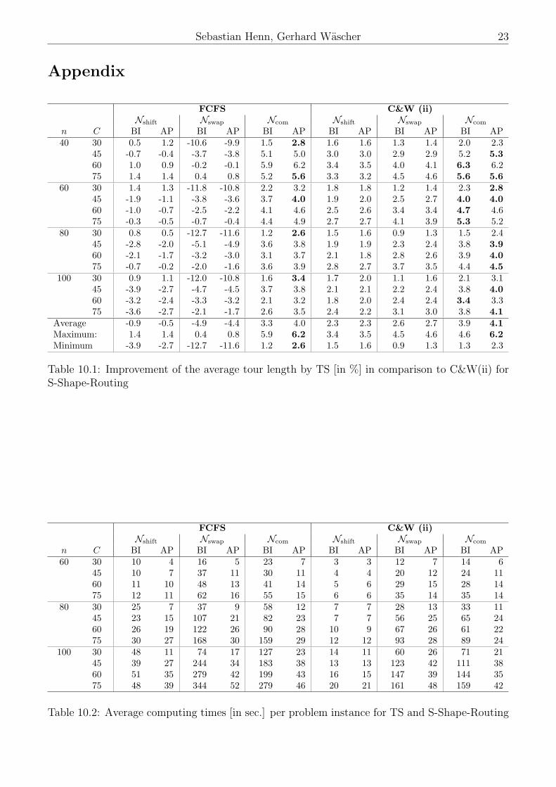
TS⋆(SSR) range from 6 seconds (60; 30) up to 42 seconds (100; 75). For a detailed view of the

average computing times per instance required by all proposed variants of TS it is referred to

Table 10.2 in the appendix. In general, increasing values of the two parameters n and C result

in increasing computing times.

The computing times observed for TS(C&W(ii)/./.) are smaller than the corresponding ones for

TS(FCFS/./.). The largest differences occur between TS(C&W(ii)/Ncom/BI) and TS(FCFS/Ncom

/BI), where - on average – the first variant consumes only 60% of the computing time of the latter

one.

Even though all neighborhood solutions obtained by the swap-operator are also included in


Ncom, the computing times for TS(./Ncom/.) are nearly identical or even smaller than those

for TS(./Nswap/.). The computing times of TS(./Nshift/.) are significantly smaller than those for

TS(./Ncom/.).

The computing times for those combinations which make use of AP are significantly smaller (cf.

problem class (100; 75)) than for those using BI, since TS(././AP) evaluates the whole neighbor-

hood of an incumbent solution, whereas TS(././AP) only considers a subset of the neighborhood

solutions.

7.2 Largest Gap-Routing

Solution Quality

For Largest Gap-Routing, TS(FCFS/Ncom/AP)(:=TS⋆(LGR)) provides the best solutions on av-

erage (average improvement: 4.1%, maximal improvement: 6.0% (40; 75), minimal improvement:

2.5% (40; 30)). In Table 10.3 in the appendix, the average improvements of the variants of TS

are depicted for those problem classes where routing is done by application of the Largest Gap-

Heuristic.

As for S-Shape-Routing, the neighborhood structure Nswap does not result to an improvement as

long as the initial solution is generated by means of FCFS. In contrast to the results for S-Shape-

Routing, independent of the initial solution, improvements of more than 2.0% can be observed for

TS(./Nshift/.). Differences obtained by application of the two initial solutions are only significant

if the neighborhood structure Nswap is applied.

As for the three neighborhood structures, those variants of TS provide the largest improvements

which include Ncom.

Concerning the size of the generated neighbourhood, the algorithms featuring AP and BI do not

provide significantly different average improvements. It should be noted, that for problem classes

with a small capacity of the picking device, AP results in more significant improvements than BI

does (cf. problem class (100; 30)).

Computing Times

The average computing times for the best performing method TS⋆(LGR) range from 12 seconds

(60; 30) up to 109 seconds (100; 75) per problem instance. The ratios of the computing times

required by the different variants to each other is in the case of Largest Gap-Routing similar to

the one observed for S-Shape-Routing (cf. Table 10.4 in the appendix).


8 Configuration Pretests for ABHC

8.1 S-Shape-Routing

Solution Quality

On average, of all variants of ABHC, ABHC(C&W(ii)/Ncom/Ao, o)(:=ABHC⋆) provides the short-

est total tour lengths (average improvement: 4.6%, maximal improvement 6.2%, minimal im-

provement: 3.7%). A detailed view of the average improvements over C&W(ii) for all considered

configurations is given in the appendix (c.f. Table 10.5).

As has already been observed during the configuration pretests for TS, the impact of the initial

solution is pivotal for the solution quality if Nshift or Nswap are used. If neighborhood solutions

are obtained by shifts and swaps, the impact of the initial solution diminish.

For the three neighborhood structures, an increase in the capacity of the picking device re-

duces the improvements obtained by ABHC(./Nshift/.), whereas the improvements obtained by

ABHC(./Nswap/.) tend to grow with an increase of the capacity. Nevertheless, ABHC(./Nshift/.)

and ABHC(./Nswap/.) are outperformed by ABHC(./Ncom/.).

Application of ABHC(././Ao, o) leads to higher improvements than ABHC(././Alexb, o) does; the

difference amounts approximately to an average of 0.4 percentage points.

Computing Times

The average computing times per problem instance for all considered variants of ABHC are pre-

sented in Table 10.6 in the appendix. Due to neglectable times for classes of small instances,

only the results for problem classes with more than 40 customer orders are listed. For the best

performing combination ABHC⋆, the computing times range from 13 seconds (60; 30) up to 188

seconds (100; 45).

Similar to the computing times of TS, those variants, which incorporate C&W(ii) for the gener-

ation of the initial solution, terminate faster than the corresponding variants which use FCFS.

If the neighborhood structure Nshift is used, ABHC(./Nshift/.) stops after at most 14 sec-

onds, whereas the other two neighborhood structures lead to computing times at least 10 times

larger. Similar to the variants of TS, ABHC(./Nswap/.) results in longer computing times than

ABHC(./Ncom/.) does.

Comparing the two attribute sets, an increase of the capacity induces larger computing times of

ABHC(././Ao, o). Using the attribute set Alexb, o, an increase of the capacity tends to reduce the

computing times. This is due to the fact that a higher capacity reduces the number of necessary

batches and, therefore, reduces the number of batch-order-combinations.



Solution Quality

The improvements of the ABHC variants (cf. Table 10.7) for Largest Gap-Routing are of very

similar size and structure as those for S-Shape-Routing. Therefore, a detailed description is

omitted, here. Again, ABHC(C&W(ii)/Ncom/Ao, o) can be identified as the best performing

variant with an average improvement of 4.6% over to the solutions provided by C&W(ii). The

improvements range from 3.5% (40; 30) to 6.1% (40; 75).

Computing Times

The computing times of the best performing ABHC variant vary between 28 (60; 30) and 500

(100; 75) seconds (cf. Table 10.8). As has already been observed for the solution quality, also

for the computing times it can be stated that the ratios of the computing times required by the

variants to each other remains valid, if the routes are determined by the Largest Gap-Heuristic.

9 Comparative Tests

9.1 Benchmarks

In order to evaluate the solution quality and the necessary computing times of the best perform-

ing Tabu Search and Attributed-Based Hill Climber variants, the performance of the proposed

methods is compared to that of several other batching strategies.

In order to provide a classical local search method against which TS and ABHC can be bench-

marked, we combine C&W(ii) with a simple local search procedure. In this local search procedure

the neighborhood structure Ncom is used and a best improvement strategy is applied. This method

will be denoted as LS, i.e. LS:=LS(C&W(ii)/Ncom/BI)).

As a further benchmark we consider the Iterated Local Search approach of Henn et al. (2009).

The heuristic consists of two alternating phases, a local search and a perturbation phase. A

first incumbent solution is generated by means of FCFS and then improved by a local search

phase. This phase is characterized by the application of a variable neighborhood descent method

with two neighborhood structures (Nshift and Nswap) and a first improvement strategy (FI). The

solution stemming from this local search phase has to pass an acceptance criterion in order to

become the next incumbent solution, otherwise the previous solution remains the incumbent solu-

tion. This solution is partially modified in the perturbation phase by randomly chosen exchanges

of customer orders assigned to different batches. This solution serves as initial solution for the

next local search phase. For a fair comparison we consider a different termination condition as

proposed by Henn et al. (2009). After n local search phases without an improvements of the

best known total tour lengths, a deterioration of the objective function value of the incumbent

solution can be accepted. The algorithm terminates after 10 deteriorations. All other parameters

of the algorithm are chosen identically to Henn et al. (2009). This algorithm is denoted by ILS-1,


Routing-Scheme n C ∅ no. of batches no. of opt. sol. ∅ Gap [%]S-Shape 40 30 2436 40 0.00

45 39295 39 1.2560 354256 16 3.1975 - - -

Largest Gap 40 30 2731 40 0.0045 32147 37 1.1360 465547 15 2.2675 - - -

Table 9.1: Optimal Solutions for S-Shape- and Largest-Gap-Routing

i.e. ILS-1:=ILS(FCFS/Ncom/FI).

Furthermore, in order to provide another benchmark a second variant of ILS (denoted by ILS-

2) has been implemented. Whereas the perturbation phase, the acceptance criterion and the

termination condition of ILS-1 remain unchanged, the initial solution is generated by means of

C&W(ii). In the local search phase the neighborhood structure Ncom is used and a best improve-

ment strategy is applied, i.e. ILS-2:=ILS(C&W(ii)/Ncom/BI).

In order to provide further insights into the solution quality of TS and ABHC, we have also tried

to benchmark their solutions against the corresponding optimal objective function values. When-

ever possible, the respective Integer Program (cf. Section 2) was generated and solved by CPLEX

10.1. This approach was only successful for a limited number of instances of the problem classes

with n = 40. Table 9.1 depicts the results obtained for these problem classes. It is shown for how

many instances CPLEX was able to generate a solution and prove its optimality (no. of opt. sol.).

For the remaining instances CPLEX was not able to prove the optimality of the solution due to

memory restrictions. For these instances the average gap between the lower bound and the best

found objective function value is presented. Furthermore, the average number of feasible batches

per problem instance is given, which corresponds to the number of columns of the mathematical

model.

9.2 S-Shape-Routing

Solution Quality

In Table 9.2 the solution quality of the best performing TS and ABHC configurations (TS⋆(SSR)

= TS(C&W(ii)/Ncom/AP); ABHC⋆=ABHC(C&W(ii)/Ncom/Ao, o)) is compared to the results of

the benchmark heuristics. For the problem classes in which the routing schemes are provided by

the S-Shape-Heuristic, LS – in comparison to C&W(ii) – achieves a reduction of the total tour

length of less than one percentage point on average. The reduction varies from 0.2% (80; 30) to

1.9% (40; 60). Therefore, it can be concluded that the solutions provided by C&W(ii) are already

close to local minima and a significant improvement by means of a simple Local Search algorithm

cannot be obtained.

By application of the two proposed implementations of ILS, total tour lengths are obtained which,

on average, are 3.0% (ILS-1) and 3.2% (ILS-2) shorther than the tour lengts of the solutions


provided by C&W(ii). For ILS-1 these improvements vary between 1.2% (100; 60) and 5.1% (40;

75). The smallest reduction obtained by ILS-2 amounts to 1.6% (100; 60), and the largest one

to 5.2% (40; 75). With respect to these small differences, it can be concluded that the impact

of the exploration of the neighborhood, which is different in both applications, is neglectable.

With respect to the proposed benchmark heuristics, significantly smaller tour lengths can be

obtained by application of TS⋆(SSR) and ABHC⋆. In comparison to ILS, on average, additional

improvements of 0.9 percentage points can be achieved by TS⋆(SSR) and 1.4 percentage points

by ABHC⋆. For TS⋆(SSR) these improvements are larger than -0.7 percentage points (60; 30)

and smaller than 1.7 percentage points (100; 60). The additional improvements of ABHC⋆ exceed

0.6 percentage points (40; 75) and are smaller than 2.1 percentage points (100; 60).

Comparing TS⋆(SSR) and ABHC⋆ to each other exclusively ABHC⋆ provides smaller total tour

lengths on average. For 15 problem classes, ABHC⋆ finds better solutions than TS⋆(SSR) does.

The largest deviations between both approaches occur for small capacities of the picking device

(cf. problem classes with C = 30).

Table 9.3 relates the solution quality of TS⋆(SSR) and ABHC⋆ to the corresponding optimal

objective function values. For all problem classes, TS⋆(SSR) and ABHC⋆ provide solutions close

to the optimum. The average deviation from the optimal objective function value (related to the

instances in each class which could be solved to a proven optimum) is smaller than two percent.

For ABHC⋆ the average deviation from the optimal objective function value tends to be smaller

for problems with a smaller capacity of the picking device than for those with a larger capacity.

In the brackets of the third and forth column of Table 9.3 the average deviations between the

objective function values provided by TS⋆/ABHC⋆and those obtained by CPLEX are presented.

These entries includue those instances in which the optimality of the obtained solution could not

n C LS ILS-1 ILS-2 TS⋆(SSR) ABHC⋆

40 30 0.3 3.1 2.8 2.3 3.845 1.1 4.5 4.3 5.3 5.360 1.9 5.1 5.0 6.2 6.275 1.2 5.0 5.2 5.6 5.8

60 30 0.3 3.4 3.5 2.8 4.345 0.6 2.7 3.0 4.0 4.460 0.8 2.9 3.4 4.6 4.875 1.2 3.5 4.0 5.2 5.4

80 30 0.2 2.9 3.0 2.4 3.745 0.6 2.3 2.4 3.9 4.260 0.7 2.1 2.4 4.0 4.275 1.1 2.5 3.0 4.5 4.5

100 30 0.2 3.0 3.4 3.1 4.245 0.4 2.2 2.3 4.0 4.460 0.6 1.2 1.6 3.3 3.775 0.7 1.2 2.4 4.1 4.2

Average 0.8 3.0 3.2 4.1 4.6Maximum: 1.9 5.1 5.2 6.2 6.2Minimum 0.2 1.2 1.6 2.3 3.7

Table 9.2: Improvement of the average tour length by TS⋆(SSR), ABHC⋆, and benchmark heuris-tics [in %] in comparison to C&W(ii) for S-Shape-Routing


n C dev. of TS⋆(SSR) dev. of ABHC⋆

40 30 1.61 (1.61) 0.09 (0.09)45 0.78 (0.76) 0.74 (0.73)60 1.74 (0.74) 1.43 (0.72)75 - -

Table 9.3: Average deviation of the total tour length obtained by TS⋆(SSR)/ABHC⋆ from theoptimal total tour length [in %]; in brackets: average deviation of the objective function value ofTS⋆(SSR)/ABHC⋆ from the objective function value provided by CPLEX for S-Shape-Routing

be proven. For some of these instances, the heuristics generate solutions with a smaller total

tour lengths than those provided by CPLEX. Therefore, the obtained average deviation is smaller

than the deviation between the total tour lengths provided by TS⋆(SSR)/ABHC⋆ and the optimal

ones.

Computing Times

The average computing times per problem instance for the benchmark heuristics, TS⋆(SSR) and

ABHC⋆ are presented in Table 9.4. For ILS-1 the time varies between 9 seconds (60; 30) and 155

seconds (100; 75), and for ILS-2 between 19 seconds (60; 30) and 246 seconds (100; 45). Due to

the exploration of the entire neighborhood, ILS-2 proves to be the most time consuming variant

of ILS.

Comparing the computing times of ILS and TS⋆(SSR) to each other consumes up to 50% of the

computing times required by ILS and provides better solutions than ILS does. The differences

between ILS and ABHC⋆ are not significant (up to 60 seconds) and involve higher quality solutions

of ABHC⋆. TS⋆(SSR) requires significantly smaller computing times than ABHC⋆ (around 20%

for the problem classes with 100 customer orders). Comparing the computing times of TS⋆(SSR)

and ABHC⋆, the TS variant already terminates after 34% of the computing time of the best

ABHC variant, on average

It can be concluded that for a large capacity of the picking device, TS⋆(SSR) provides similar,

n C LS ILS-1 ILS-2 TS⋆(SSR) ABHC⋆

60 30 0 9 19 6 1345 0 18 33 11 2260 0 21 30 14 2275 0 22 34 14 25

80 30 0 31 46 11 4545 0 62 91 24 7860 0 64 89 22 6975 0 68 96 24 82

100 30 0 68 135 21 12645 1 129 246 38 18860 1 138 170 35 17875 1 155 173 42 180

Table 9.4: Average computing times [in sec.] per problem instance of TS⋆(SSR), ABHC⋆, andbenchmark heuristics for S-Shape-Routing


high quality solutions in shorter computing times than ABHC⋆does, whereas, for small capacities,

the larger computing times of ABHC⋆ are justified by a significantly larger improvement of the

total tour length.


Solution Quality

n C LS ILS-1 ILS-2 TS⋆(LGR) ABHC⋆

40 30 0.3 2.9 2.4 1.1 3.545 0.6 3.1 3.1 3.8 3.860 1.0 4.4 4.2 4.8 4.875 1.8 5.7 5.5 6.2 6.1

60 30 0.2 2.8 2.6 1.1 3.745 0.5 2.9 2.9 3.6 3.760 0.9 4.1 4.4 5.0 5.175 1.4 5.3 5.5 6.2 6.1

80 30 0.1 3.0 2.9 0.3 4.045 0.5 2.5 2.8 3.2 3.760 0.7 3.4 3.6 4.4 4.575 1.0 4.5 4.9 5.5 5.8

100 30 0.1 2.9 3.0 0.8 4.245 0.4 2.6 2.7 3.7 3.960 0.6 3.0 3.2 4.4 4.475 0.9 4.6 4.9 5.5 5.8

Average 0.7 3.6 3.7 3.7 4.6Maximum: 1.8 5.7 5.5 6.2 6.1Minimum 0.1 2.5 2.4 0.3 3.5

Table 9.5: Improvement of the average tour length by TS⋆(LGR), ABHC⋆, and benchmark heuris-tics [in %] in comparison to C&W(ii) for Largest Gap-Routing

Table 9.5 compares the best performing TS and ABHC variants (TS⋆(LGR)=TS(FCFS/Ncom/BI);

ABHC⋆ = ABHC(C&W(ii)/Ncom/Ao, o)) to the benchmark heuristics for Largest Gap-Routing.

The improvements of C&W(ii)+LS as compared to C&W(ii) are of similar size as in the case of S-

Shape-Routing. Likewise the ratios of the improvements among the ILS variants but also between

the ILS variants and ABHC⋆ are almost identical to the S-Shape case. Consequently, details will

not be presented here. On average, the application of TS⋆(LGR) leads to an improvement similar

to that of ILS (TS⋆(LGR): 3.7%; ILS-1: 3.6%; ILS-2: 3.7%), even though the spread of the

improvements may differ significantly across the problem classes. For a small capacity (C = 30),

TS⋆(LGR) is not able to provide improvements of more than 1.1%, whereas, for a large capacity

(C = 100), the improvements are the best ones observed at all. ABHC⋆ outperforms TS⋆(LGR)

in 12 problem classes.

The solution quality of TS⋆(LGR) and ABHC⋆ is presented in Table 9.6, which depicts the

average deviation of the obtained total tour lengths from the optimal ones. Similar to the case

of S-Shape-Routing, the average deviation is small for ABHC⋆ (less than 0.4%). For a large

capacity, TS⋆(LGR) provides solutions with tour lengths, which differ at most 0.73% from the


n C TS⋆(LGR) ABHC⋆

40 30 2.74 (2.74) 0.24 (0.24)45 0.37 (0.34) 0.39 (0.36)60 0.73 (0.14) 0.38 (0.09)75 - -

Table 9.6: Average deviation of the total tour length obtained by TS⋆(SSR)/ABHC⋆ from theoptimal total tour length [in %]; in brackets: average deviation of the objective function valueof TS⋆(LGR)/ABHC⋆ from the objective function value provided by CPLEX for Largest Gap-Routing

optimal objective function values. In class (40; 30), the difference of TS⋆(LGR) to the optimal

total tour lengths amounts to 2.74%.

Computing Times

The average computing times are shown in Table 9.7, where only the results for problem classes

with more than 40 customer orders are presented. Due to the higher computational effort required

by the Largest Gap-Heuristic, these computing times are larger than in the case of S-Shape-

Routing. Among the investigated metaheuristics TS⋆(LGR) provides solutions in the shortest

time, whereas ABHC⋆ requires computing times of up to 500 seconds.

n C LS ILS-1 ILS-2 TS⋆(LGR) ABHC⋆

60 30 0 21 32 12 2845 0 43 65 20 5260 0 52 71 25 5575 1 60 80 30 57

80 30 0 71 118 27 10645 1 118 209 41 16760 1 151 232 47 17475 1 169 273 62 178

100 30 1 166 281 47 31745 1 299 511 61 42460 2 322 491 76 43275 2 397 569 109 500

Table 9.7: Average computing times [in sec.] per problem instance of TS⋆(LGR), ABHC⋆, andbenchmark heuristics for Largest Gap-Routing

10 Conclusions and Outlook

This paper dealt with the Order Batching Problem, a problem pivotal for the efficient management

and control of manual picker-to-parts order picking systems in distribution warehouses. For the

solution of this problem two metaheuristics have been applied, namely Tabu Search and the

Attribute-Based Hill Climber. For each of these two heuristics we analyzed the performance of

different configurations in extensive numerical experiments. By means of comparing the proposed

methods to selected benchmark heuristics it was shown that both approaches generate improved


solutions of similar quality. Furthermore, the computing times of both approaches are significantly

smaller than the ones of existing solution approaches, which provide similar total tour lengths.

Therefore, both variants appear very suitable for being implemented in software systems for

practical purposes. The application of both approaches can reduce the total tour length, and

consequently result in a reduction of the overall picking time. This might allow even for a

reduction of overtimes or for a reduction of the workforce, both critical aspects in warehouse

environments where low profit margins prevail. Furthermore, the improved solutions can result

in shorter lead times in picking customer orders, and, thus, in an improved customer service.

Future research should concentrate on the adaption of these powerful metaheuristics for dynamic

warehouse environments. In theses situations, customer orders arrive over time and a huge number

of batching steps is necessary.


References

Bozer, Y. and J. Kile (2008). Order Batching in Walk-and-Pick Order Picking Systems. Inter-

national Journal of Production Research 46 (7), 1887–1909.

Caron, F., G. Marchet, and A. Perego (1998). Routing Policies and COI-Based Storage Policies

in Picker-to-Part Systems. International Journal of Production Research 36 (3), 713–732.

Chen, M.-C. and H.-P. Wu (2005). An Association-Based Clustering Approach to Order Batch-

ing Considering Customer Demand Patterns. Omega - International Journal of Management

Science 33 (4), 333–343.

Clarke, G. and J. Wright (1964). Scheduling of Vehicles from a Central Depot to a Number of

Delivery Points. Operations Research 12 (4), 568–581.

de Koster, M., E. van der Poort, and M. Wolters (1999). Efficient Orderbatching Methods in

Warehouses. International Journal of Production Research 37 (7), 1479–1504.

de Koster, R., K. Roodbergen, and R. van Voorden (1999). Reduction of Walking Time in the

Distribution Center of De Bijenkorf. In M. Speranza and P. Stahly (Eds.), New Trends in

Distribution Logistics, pp. 215–234. Berlin: Springer.

Derigs, U. and R. Kaiser (2007). Applying the Attribute Based Hill Climber Heuristic to the

Vehicle Routing Problem. European Journal of Operational Research 177 (2), 719–732.

Derigs, U. and K. Reuter (2009). A Simple and Efficient Tabu Search Heuristic for Solving the

Open Vehicle Routing Problem. Journal of the Operational Research Society 60, 1658–1669.

Elsayed, E. (1981). Algorithms for Optimal Material Handling in Automatic Warehousing Sys-

tems. International Journal of Production Research 19 (5), 525–535.

Elsayed, E. and R. Stern (1983). Computerized Algorithms for Order Processing in Automated

Warehousing Systems. International Journal of Production Research 21 (4), 579–586.

Elsayed, E. and O. Unal (1989). Order Batching Algorithms and Travel-Time Estimation for

Automated Storage/Retrieval Systems. International Journal of Production Research 27 (7),

1097–1114.

Frazelle, E. (2002). World-Class Warehousing and Material Handling. New York: McGraw-Hill.

Gademann, N. and S. van de Velde (2005). Order Batching to Minimize Total Travel Time in a

Parallel-Aisle Warehouse. IIE Transactions 37 (1), 63–75.

Gibson, D. and G. Sharp (1992). Order Batching Procedures. European Journal of Operational

Research 58 (1), 57–67.


Glover, F. (1986). Future Paths for Integer Programming and Links to Artificial Intelligence.

Computers and Operations Research 13 (5), 533–549.

Glover, F. and M. Laguna (1997). Tabu Search. Kluwer Academic Publishers.

Henn, S., S. Koch, K. Doerner, C. Strauss, and G. Wascher (2009). Metaheuristics for the

Order Batching Problem in Manual Order Picking Systems. Working Paper 20/2009, Faculty

of Economics and Management, Otto-von-Guericke-University Magdeburg.

Ho, Y.-C., T.-S. Su, and Z.-B. Shi (2008). Order-Batching Methods for an Order-Picking Ware-

house with two Cross Aisles. Computers & Industrial Engineering 55 (2), 321–347.

Ho, Y.-C. and Y.-Y. Tseng (2006). A Study on Order-Batching Methods or Order-Picking in a Dis-

tribution Center with two Cross Aisles. International Journal of Production Research 44 (17),

3391–3417.

Hsu, C., K. Chen, and M. Chen (2005). Batching Orders in Warehouses by Minimizing Travel

Distance with Genetic Algorithms. Computers in Industry 56 (2), 169–178.

Jarvis, J. and E. McDowell (1991). Optimal Product Layout in an Order Picking Warehouse. IIE

Transactions 23 (1), 93–102.

Pan, C. and S. Liu (1995). A Comparative Study of Order Batching Algorithms. Omega -

International Journal of Management Science 23 (6), 691–700.

Petersen, C. and R. Schmenner (1999). An Evaluation of Routing and Volume-based Storage

Policies in an Order Picking Operation. Decision Sciences 30 (2), 481–501.

Tompkins, J., J. White, Y. Bozer, and J. Tanchoco (2003). Facilities Planning (3th edition ed.).

New Jersey: John Wiley & Sons.

Tsai, C.-Y., J. Liou, and T.-M. Huang (2008). Using a Multiple-GA Method to Solve the Batch

Picking Problem: Considering Travel Distance and Order Due Time. International Journal of

Production Research 46 (22), 6533–6555.

Wascher, G. (2004). Order Picking: A Survey of Planning Problems and Methods. In H. Dyckhoff,

R. Lackes, and J. Reese (Eds.), Supply Chain Management and Reverse Logistics, pp. 323–347.

Berlin et al.: Springer.

Whittley, I. and G. Smith (2004). The Attribute Based Hill Climber. Journal of Mathematical

Modelling and Algorithms 3 (2), 167–178.

Yu, M. and R. de Koster (2009). The Impact of Order Batching and Picking Area Zoning on Order

Picking System Performance. European Journal of Operational Research 198 (2), 480–490.


Appendix

FCFS C&W (ii)Nshift Nswap Ncom Nshift Nswap Ncom

n C BI AP BI AP BI AP BI AP BI AP BI AP40 30 0.5 1.2 -10.6 -9.9 1.5 2.8 1.6 1.6 1.3 1.4 2.0 2.3

45 -0.7 -0.4 -3.7 -3.8 5.1 5.0 3.0 3.0 2.9 2.9 5.2 5.360 1.0 0.9 -0.2 -0.1 5.9 6.2 3.4 3.5 4.0 4.1 6.3 6.275 1.4 1.4 0.4 0.8 5.2 5.6 3.3 3.2 4.5 4.6 5.6 5.6

60 30 1.4 1.3 -11.8 -10.8 2.2 3.2 1.8 1.8 1.2 1.4 2.3 2.845 -1.9 -1.1 -3.8 -3.6 3.7 4.0 1.9 2.0 2.5 2.7 4.0 4.060 -1.0 -0.7 -2.5 -2.2 4.1 4.6 2.5 2.6 3.4 3.4 4.7 4.675 -0.3 -0.5 -0.7 -0.4 4.4 4.9 2.7 2.7 4.1 3.9 5.3 5.2

80 30 0.8 0.5 -12.7 -11.6 1.2 2.6 1.5 1.6 0.9 1.3 1.5 2.445 -2.8 -2.0 -5.1 -4.9 3.6 3.8 1.9 1.9 2.3 2.4 3.8 3.960 -2.1 -1.7 -3.2 -3.0 3.1 3.7 2.1 1.8 2.8 2.6 3.9 4.075 -0.7 -0.2 -2.0 -1.6 3.6 3.9 2.8 2.7 3.7 3.5 4.4 4.5

100 30 0.9 1.1 -12.0 -10.8 1.6 3.4 1.7 2.0 1.1 1.6 2.1 3.145 -3.9 -2.7 -4.7 -4.5 3.7 3.8 2.1 2.1 2.2 2.4 3.8 4.060 -3.2 -2.4 -3.3 -3.2 2.1 3.2 1.8 2.0 2.4 2.4 3.4 3.375 -3.6 -2.7 -2.1 -1.7 2.6 3.5 2.4 2.2 3.1 3.0 3.8 4.1

Average -0.9 -0.5 -4.9 -4.4 3.3 4.0 2.3 2.3 2.6 2.7 3.9 4.1Maximum: 1.4 1.4 0.4 0.8 5.9 6.2 3.4 3.5 4.5 4.6 4.6 6.2Minimum -3.9 -2.7 -12.7 -11.6 1.2 2.6 1.5 1.6 0.9 1.3 1.3 2.3

Table 10.1: Improvement of the average tour length by TS [in %] in comparison to C&W(ii) forS-Shape-Routing


n C BI AP BI AP BI AP BI AP BI AP BI AP60 30 10 4 16 5 23 7 3 3 12 7 14 6

45 10 7 37 11 30 11 4 4 20 12 24 1160 11 10 48 13 41 14 5 6 29 15 28 1475 12 11 62 16 55 15 6 6 35 14 35 14

80 30 25 7 37 9 58 12 7 7 28 13 33 1145 23 15 107 21 82 23 7 7 56 25 65 2460 26 19 122 26 90 28 10 9 67 26 61 2275 30 27 168 30 159 29 12 12 93 28 89 24

100 30 48 11 74 17 127 23 14 11 60 26 71 2145 39 27 244 34 183 38 13 13 123 42 111 3860 51 35 279 42 199 43 16 15 147 39 144 3575 48 39 344 52 279 46 20 21 161 48 159 42

Table 10.2: Average computing times [in sec.] per problem instance for TS and S-Shape-Routing



n C BI AP BI AP BI AP BI AP BI AP BI AP40 30 0.7 2.3 -9.1 -8.7 1.1 2.5 1.2 1.0 0.7 1.0 1.2 1.6

45 2.1 2.0 -3.6 -3.6 3.8 3.8 2.6 2.7 1.9 1.8 3.8 3.860 2.5 2.6 -0.4 -0.5 4.8 4.6 3.3 3.2 3.5 3.3 4.8 4.775 4.5 4.5 2.2 2.1 6.2 6.0 4.8 4.7 5.0 5.0 6.2 6.1

60 30 0.7 2.4 -9.5 -9.2 1.1 2.9 1.1 0.9 0.5 0.8 0.6 1.345 0.9 1.2 -3.6 -3.7 3.6 3.5 2.0 2.0 2.3 2.3 3.6 3.560 2.4 2.3 0.1 -0.2 5.0 4.8 3.2 3.2 3.6 3.5 5.0 4.875 3.9 3.8 1.6 1.4 6.2 5.8 4.0 4.2 4.7 4.5 6.3 5.8

80 30 -0.2 2.8 -11.3 -10.9 0.3 2.9 0.8 0.7 0.5 0.9 0.8 1.445 0.0 0.5 -4.1 -4.3 3.2 3.3 2.0 2.0 2.0 1.9 3.4 3.460 1.3 1.2 -1.0 -1.5 4.4 4.2 2.6 2.5 3.3 3.2 4.5 4.375 2.3 2.3 1.3 0.8 5.5 5.3 3.6 3.6 4.8 4.6 5.7 5.4

100 30 0.4 2.9 -10.7 -10.3 0.8 3.3 0.8 1.0 0.5 1.1 0.8 1.745 0.6 0.6 -3.9 -4.2 3.7 3.4 1.9 1.8 2.2 2.1 3.8 3.660 0.4 0.7 -1.0 -1.5 4.4 3.9 2.5 2.5 3.1 2.9 4.4 4.175 2.0 2.0 1.4 0.9 5.5 5.3 3.6 3.7 4.8 4.6 5.8 5.4

Average 1.5 2.1 -3.2 -3.3 3.7 4.1 2.5 2.5 2.7 2.7 3.8 3.8Maximum: 4.5 4.5 2.2 2.1 6.2 6.0 4.8 4.7 5.0 5.0 6.3 6.1Minimum -0.2 0.5 -11.3 -10.9 0.3 2.5 0.8 0.7 0.5 0.8 0.6 1.3

Table 10.3: Improvement of the average tour length by TS [in %] in comparison to C&W(ii)Largest Gap-Routing


n C BI AP BI AP BI AP BI AP BI AP BI AP60 30 21 11 28 8 40 12 8 7 24 12 26 10

45 27 21 80 19 66 20 11 8 47 22 49 1760 26 22 106 27 80 25 14 12 66 30 62 2475 26 23 131 30 96 30 16 14 77 33 68 27

80 30 49 24 65 17 91 27 16 12 51 26 57 2145 66 40 227 34 154 41 17 18 131 42 108 4160 63 46 285 45 193 47 24 21 145 54 147 4775 66 54 307 55 236 62 34 28 189 65 167 58

100 30 88 37 127 26 184 47 28 23 104 47 117 3445 150 59 446 53 336 61 33 29 232 69 234 6460 98 86 519 69 382 76 37 39 309 82 254 7875 120 103 610 97 486 109 54 50 372 103 344 88

Table 10.4: Average computing times [in sec.] per problem instance for TS and Largest Gap-Routing



n C Ao,o Alexb,o Ao,o Alex

b,o Ao,o Alexb,o Ao, o Alex

b,o Ao,o Alexb,o Ao,o Alex

b,o

40 30 1.7 1.8 -9.2 -9.2 3.8 3.7 2.1 2.4 1.9 1.8 3.8 3.845 -1.8 -2.0 -3.5 -3.7 5.5 5.0 2.1 2.4 3.1 2.8 5.3 5.160 -0.5 -1.2 -0.1 -0.5 6.3 5.6 2.7 2.6 4.1 3.8 6.2 5.675 0.4 -0.8 0.9 -0.1 5.5 4.7 2.7 2.4 5.0 4.2 5.8 4.9

60 30 1.6 1.9 -10.2 -10.2 4.3 4.2 2.7 2.6 2.2 2.1 4.3 4.245 -4.0 -3.8 -3.2 -3.6 4.6 4.0 1.6 1.7 3.0 2.7 4.4 3.960 -2.1 -2.5 -1.7 -2.3 4.9 4.2 1.9 1.9 3.6 3.3 4.8 4.575 -2.4 -2.2 0.1 -0.6 5.2 4.0 2.3 2.2 4.2 3.7 5.4 4.9

80 30 1.2 1.7 -11.0 -11.0 3.7 3.7 2.0 2.3 2.0 1.9 3.7 3.645 -4.7 -4.1 -4.4 -4.7 4.2 4.0 1.4 1.4 2.8 2.5 4.2 4.060 -3.8 -3.2 -2.0 -2.7 4.1 3.4 1.5 1.5 3.1 2.8 4.2 4.075 -3.2 -3.4 -0.6 -1.6 4.5 3.4 2.3 2.1 4.0 3.5 4.5 4.2

100 30 1.7 2.0 -10.2 -10.3 4.2 4.2 2.2 2.5 2.2 2.1 4.2 4.245 -5.2 -4.9 -4.0 -4.2 4.3 4.0 1.5 1.7 2.7 2.4 4.4 4.060 -5.4 -4.8 -2.2 -2.9 3.5 2.9 1.3 1.6 2.9 2.5 3.7 3.475 -4.4 -4.7 -0.6 -1.5 3.8 2.8 1.7 1.7 3.4 3.0 4.2 3.9

Average -1.9 -1.9 -3.9 -4.3 4.5 4.0 2.0 2.1 3.1 2.8 4.6 4.3Maximum: 1.7 2.0 0.9 -0.1 6.3 5.6 2.7 2.6 5.0 4.2 6.2 5.6Minimum -5.4 -4.9 -11.0 -11.0 3.5 2.8 1.3 1.4 1.9 1.8 3.7 3.4

Table 10.5: Improvement of the average tour length by ABHC [in %] in comparison to C&W(ii)for S-Shape-Routing





b,o

60 30 2 1 22 36 22 14 1 2 14 18 13 1545 1 1 47 25 30 12 0 1 26 13 22 1160 2 1 52 25 33 13 1 1 27 11 22 975 2 1 55 19 35 13 1 1 29 10 25 10

80 30 7 7 81 154 78 61 2 7 44 64 45 5845 2 1 172 104 106 46 1 1 101 49 78 3660 5 3 204 97 103 50 2 2 96 35 69 2975 7 3 226 83 124 57 4 2 107 30 82 27

100 30 13 12 213 421 199 159 5 14 124 179 126 16745 3 2 432 289 274 108 1 2 257 137 188 10060 5 4 543 230 276 118 3 3 237 86 178 7575 14 6 608 219 316 122 8 5 244 72 180 61

Table 10.6: Average computing times [in sec.] per problem instance for ABHC and S-Shape-Routing






b,o

40 30 2.3 2.4 -8.2 -8.2 3.5 3.5 2.5 2.7 1.4 1.4 3.5 3.445 -0.6 -0.8 -3.5 -3.7 3.8 3.6 1.8 1.7 2.0 1.8 3.8 3.760 -0.7 -1.2 -0.4 -0.7 4.8 4.4 2.0 1.9 3.5 3.2 4.8 4.675 2.8 1.8 2.3 2.0 6.0 5.5 3.7 3.5 4.9 4.6 6.1 5.7

60 30 2.3 2.6 -8.6 -8.6 3.7 3.7 2.6 2.9 1.3 1.3 3.7 3.645 -1.7 -1.5 -3.4 -3.6 3.8 3.5 1.4 1.3 2.4 2.3 3.7 3.560 0.1 0.0 0.1 -0.2 5.0 4.6 2.4 2.4 3.6 3.3 5.1 4.875 1.3 1.2 1.8 1.2 6.1 5.8 3.5 3.3 4.7 4.4 6.1 5.8

80 30 2.2 2.7 -10.2 -10.2 4.0 4.0 2.7 2.9 1.4 1.4 4.0 3.945 -2.6 -2.8 -3.9 -4.0 3.7 3.5 1.4 1.5 2.2 2.0 3.7 3.560 -1.1 -1.6 -0.9 -1.1 4.5 4.2 2.0 1.7 3.4 3.1 4.5 4.275 0.7 0.1 1.5 1.0 5.6 5.2 2.9 2.6 4.9 4.6 5.8 5.5

100 30 2.5 2.8 -9.6 -9.6 4.2 4.1 2.7 3.1 1.5 1.5 4.2 4.245 -1.8 -2.0 -3.7 -3.9 3.9 3.7 1.3 1.4 2.4 2.2 3.9 3.860 -1.9 -2.0 -0.7 -1.0 4.5 4.3 1.9 1.9 3.3 3.0 4.4 4.375 -0.1 -0.5 1.7 1.2 5.8 5.2 2.7 2.5 5.0 4.6 5.8 5.5

Average 0.2 0.1 -2.9 -3.1 4.6 4.3 2.3 2.3 3.0 2.8 4.6 4.4Maximum: 2.8 2.8 2.3 2.0 6.1 5.8 3.7 3.5 5.0 4.6 6.1 5.8Minimum -2.6 -2.8 -10.2 -10.2 3.5 3.5 1.3 1.3 1.3 1.3 3.5 3.4

Table 10.7: Improvement of the average tour length by ABHC [in %] in comparison to C&W(ii)for Largest Gap-Routing





b,o

60 30 5 5 45 71 40 35 2 5 27 37 28 3445 2 1 103 60 65 29 1 1 56 29 52 2660 5 2 102 45 63 25 3 2 63 24 55 2475 6 3 106 41 64 24 4 3 67 25 57 22

80 30 12 9 158 281 160 125 5 9 98 121 106 11445 5 2 351 184 219 82 2 3 213 98 167 7560 9 4 382 168 204 76 5 4 216 83 174 7575 20 9 386 163 217 80 12 7 223 80 178 71

100 30 31 24 413 766 448 354 16 37 270 348 317 35545 12 6 880 498 569 214 4 6 551 264 424 20560 17 10 991 458 543 213 8 8 537 211 432 17475 42 16 1.059 432 603 206 18 10 601 211 500 178

Table 10.8: Average computing times [in sec.] per problem instance for ABHC and LargestGap-Routing

Tabu Search Heuristics for the Order Batching Problem in ...

Documents

Transcript of Tabu Search Heuristics for the Order Batching Problem in ...