2048 solving AIA reinforcement learning + neural net approach

Antoine ROUXFebruary 27, 2019

1

Contents

1 Presentation of the project 31.1 The game 2048 . . . . . . . . . . . . . . . . . . . . . . . . . . . . . . . . . . 31.2 My approach . . . . . . . . . . . . . . . . . . . . . . . . . . . . . . . . . . . 3

2 The player mode 5

3 The neural network mode 63.1 What already exists . . . . . . . . . . . . . . . . . . . . . . . . . . . . . . . 63.2 My general idea . . . . . . . . . . . . . . . . . . . . . . . . . . . . . . . . . . 63.3 Structure of the neural net . . . . . . . . . . . . . . . . . . . . . . . . . . . . 63.4 Hard-coded network weights . . . . . . . . . . . . . . . . . . . . . . . . . . . 7

3.4.1 Structure . . . . . . . . . . . . . . . . . . . . . . . . . . . . . . . . . 73.4.2 Results . . . . . . . . . . . . . . . . . . . . . . . . . . . . . . . . . . 7

4 The genetic learning algorithm 104.1 Implementation . . . . . . . . . . . . . . . . . . . . . . . . . . . . . . . . . . 104.2 Choosing the hyperparameters . . . . . . . . . . . . . . . . . . . . . . . . . 10

4.2.1 Size of a generation . . . . . . . . . . . . . . . . . . . . . . . . . . . . 114.2.2 Selection rate for best individuals . . . . . . . . . . . . . . . . . . . . 124.2.3 Selection rate for other individuals . . . . . . . . . . . . . . . . . . . 134.2.4 Mutation rate . . . . . . . . . . . . . . . . . . . . . . . . . . . . . . . 144.2.5 Number of generations . . . . . . . . . . . . . . . . . . . . . . . . . . 154.2.6 Conclusion of the choice of hyperparameters . . . . . . . . . . . . . . 16

4.3 Choosing the network structure . . . . . . . . . . . . . . . . . . . . . . . . . 164.4 A note on the randomness . . . . . . . . . . . . . . . . . . . . . . . . . . . . 174.5 Results for the chosen structure . . . . . . . . . . . . . . . . . . . . . . . . . 184.6 Conclusion of the neural net approach . . . . . . . . . . . . . . . . . . . . . 20

5 The graphical user interface 21

Conclusion and future improvements 23

2

1 Presentation of the project

1.1 The game 2048

During a course on Artificial Intelligence at ENSTA ParisTech, I discovered the evo-lutionary algorithms, and found them extremely interesting. I wanted to find a funnyway to create my own, and finally came out with the idea of re-creating the famoussmartphone game 2048.

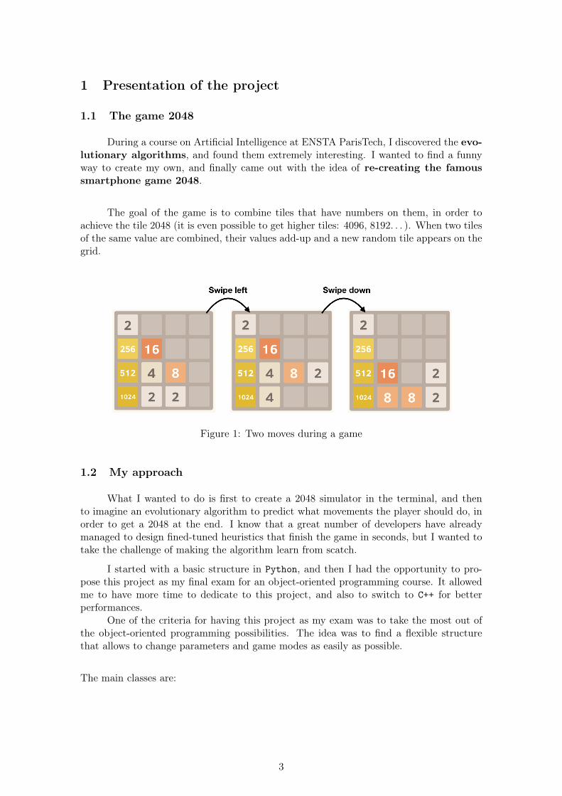
The goal of the game is to combine tiles that have numbers on them, in order toachieve the tile 2048 (it is even possible to get higher tiles: 4096, 8192. . . ). When two tilesof the same value are combined, their values add-up and a new random tile appears on thegrid.

Figure 1: Two moves during a game

1.2 My approach

What I wanted to do is first to create a 2048 simulator in the terminal, and thento imagine an evolutionary algorithm to predict what movements the player should do, inorder to get a 2048 at the end. I know that a great number of developers have alreadymanaged to design fined-tuned heuristics that finish the game in seconds, but I wanted totake the challenge of making the algorithm learn from scatch.

I started with a basic structure in Python, and then I had the opportunity to pro-pose this project as my final exam for an object-oriented programming course. It allowedme to have more time to dedicate to this project, and also to switch to C++ for betterperformances.

One of the criteria for having this project as my exam was to take the most out ofthe object-oriented programming possibilities. The idea was to find a flexible structurethat allows to change parameters and game modes as easily as possible.

The main classes are:

3

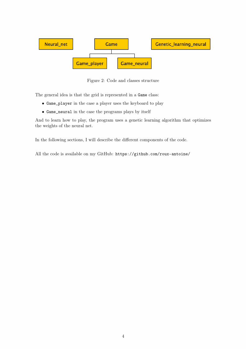
Figure 2: Code and classes structure

The general idea is that the grid is represented in a Game class:

• Game_player in the case a player uses the keyboard to play

• Game_neural in the case the programs plays by itself

And to learn how to play, the program uses a genetic learning algorithm that optimizesthe weights of the neural net.

In the following sections, I will describe the different components of the code.

All the code is available on my GitHub: https://github.com/roux-antoine/

4

2 The player mode

The basic structure is composed of a class Game, that represents the grid and itscorresponding methods (swipe, add_random_number...). There is also a play method,whose behavior is really simple :

• initialize the grid

• get the swipe direction

• if the direction is legal, swipe and update the grid

• add a random number

And that until the grid is full!

In order to take the most out of inheritance, the only thing that changes betweenthe different modes is the get_direction method.

In the case of the player mode, we have a Game_player class, whose get_directionmethod retrieves the direction the user want to swipe to, using the keyboard.

The dimension of the grid can be chosen by the user, the choices being 3, 4 of 5 tiles(more than 5 is too long to play...).(For visuals of the GUI, cf the last section.)

5

3 The neural network mode

3.1 What already exists

Since this game was fairly popular a few years back, many developers have tackled thechallenge of writing AIs able to play. Here are the main techniques used:

• Doing N random moves and seeing which one leads to the best score (as in this).That’s a funny approach, but with no learning involved.

• Checking all possible next moves (up to 1000 moves in this person’s implementation)and see which ones lead to the best score. Once again, no learning involved.

• Using heuristics coded by a human: this approach is using both ML and humanexpertise (as in this). It’s a powerful method, but it’s also interesting to learn withoutany human input

• Neural network + genetic learning: it is the approach I chose as well. It has beenimplemented by this person and this person and this person, but in all cases theirAI only manage to get around the tile 512.

3.2 My general idea

My idea to tackle the problem of choosing a move to make was as follows:

• at each step the algorithm simulates all the possible moves with a certain numberof moves in advance (between 1 and 6, denoted N and called depth). So we end upwith around 4N potential grids.

• we give each of these grids a score (called fitness) that characterizes how good thisconfiguration is. The fitness is computed using a neural network.

• we decide to do the move that gives the best fitness

3.3 Structure of the neural net

Because I needed just a rudimentary neural network library (and because I like toget my hands dirty), I created my own Neural_net class.Its attributes are:

• gridSize: the size of the grid chosen by the user (corresponding to the input layerif the network)

• nbrLayers: the number of layers in the network

• layersSizes: the width of each layer

• nonLinearities: the non-linearities of each layer

• weights: the weights of each layer

• biases: the biases of each layer

• layers: the values stored in the neurons of each layer

Its methods are:

• forward_pass: computes the output of the network for a given input grid

6

• save_to_file: saves the learned weights and biases to a .txt file

• print: prints the characteristics of the network for debugging purposes

3.4 Hard-coded network weights

3.4.1 Structure

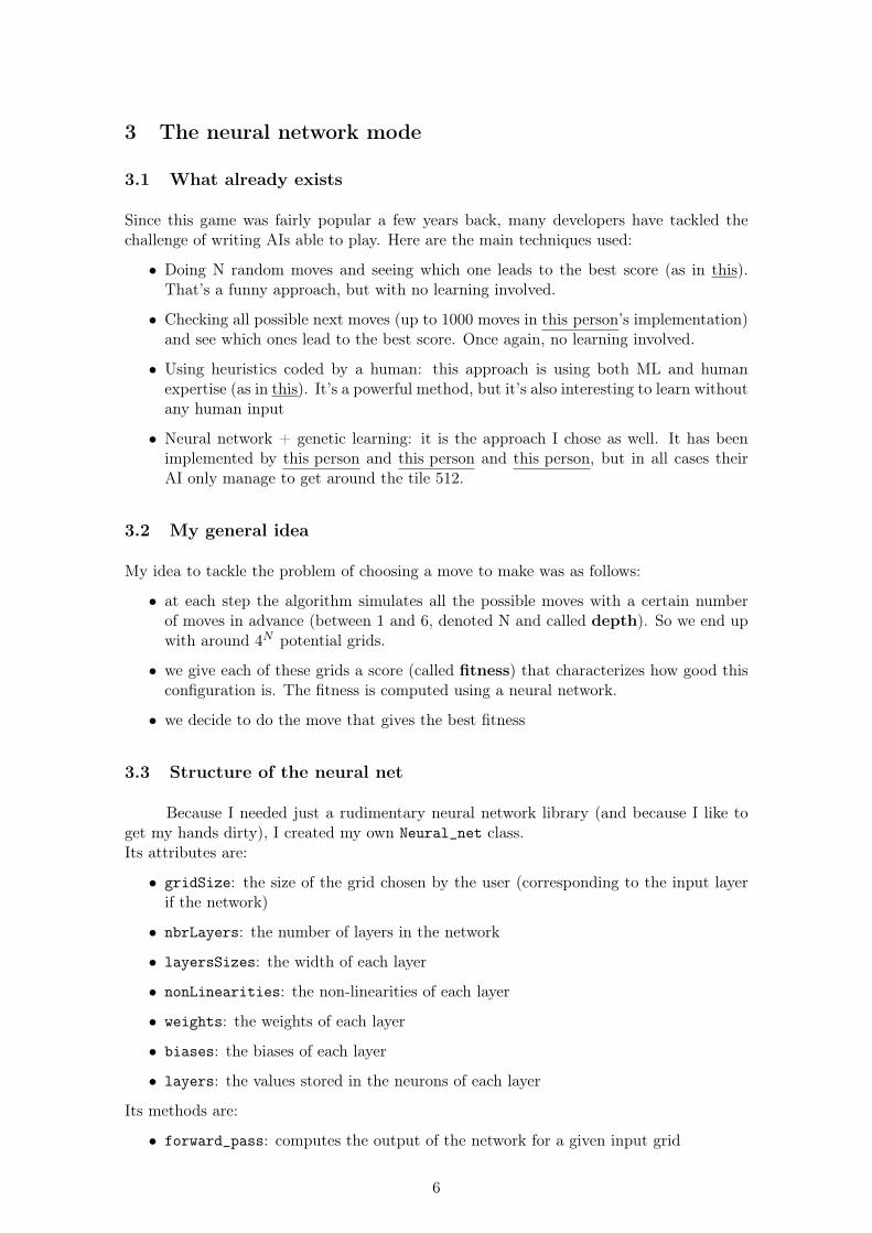
A powerful technique to achieve a high score is to sort the tiles by increasing value,with the highest in a corner. As a consequence, I designed a hard-coded neural net thathas 2 layers (the input layer having same dimension as the grid, the last being of size 1),and no non-linearity.The network returns a high fitness when the tiles are sorted on the grid (something indi-cating a favorable grid configuration).

It corresponds to the following formula for the fitness (in the case of a 4 × 4 grid):

fitness =∑4

i=1

∑4j=1AijBij

Where A is the playing grid, for instance :0 0 0 02 0 0 04 8 0 08 2 2 0

And B is the matrix obtained by stacking the weights of the first layer in a square fashion:

13 12 5 414 11 6 315 10 7 216 9 8 1

Figure 3: Representation of the hard-coded network

3.4.2 Results

This approach was the first step to see if this kind of technique could achieve 2048.

7

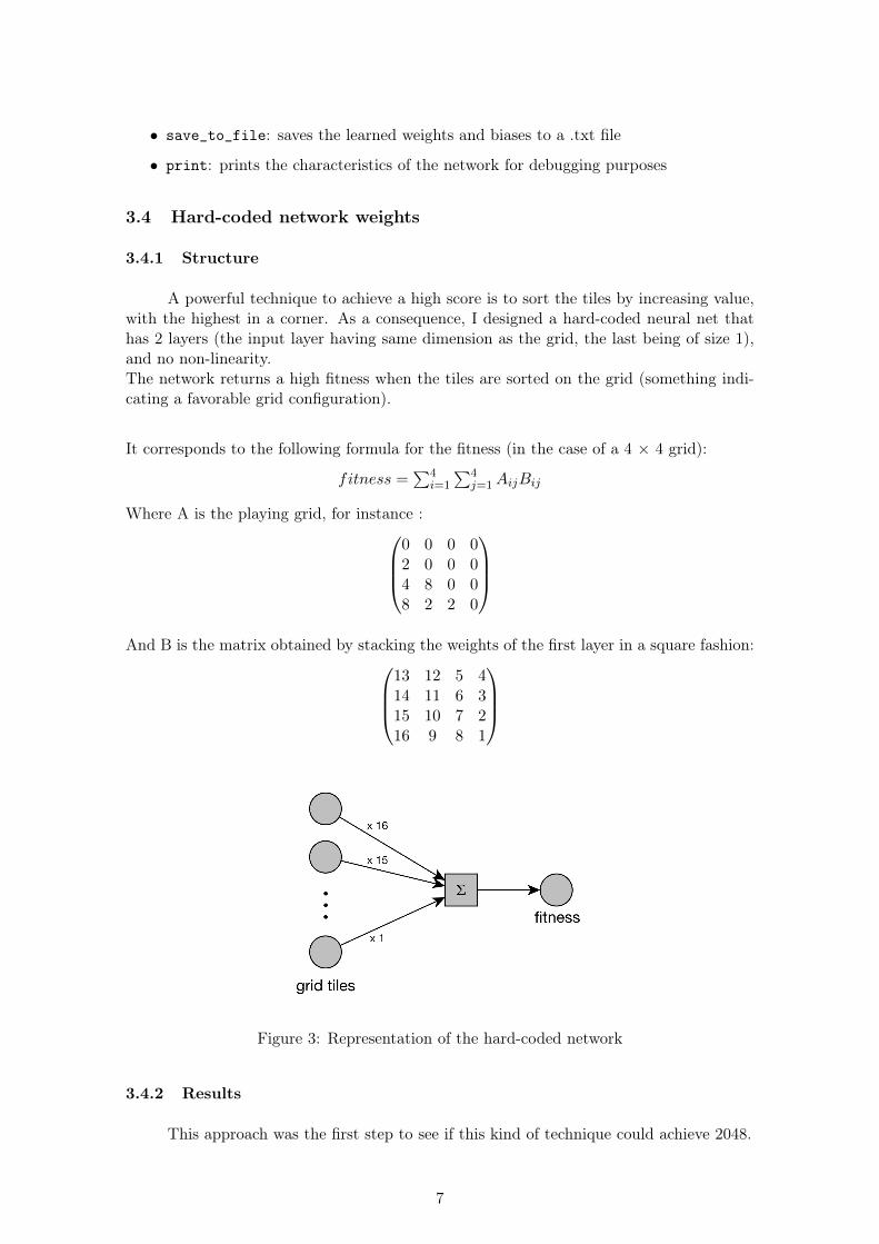
With the fitness function I wrote, the algorithm obtained quite good results. Becausethe tiles appear randomly, I evaluated the algorithm on many games (depending on thedepth), to get an average performance.Here are the results for two different depths of search:

• two moves ahead (evaluated on 10,000 games)

• six moves ahead (evaluated on 70 games)

Figure 4: Frequence of max tile value for depth 2 and 6

We can see that the AI manages to get to 2048, and even 4096 on some occasions.For a search depth of 2, the average final score is around 1600 (a value that I will comparewith the performance of the genetic learning algorithm later). The limitation here is thefitness function that I have coded.We can also see that the algorithm gets better as depth increases, which is logical.

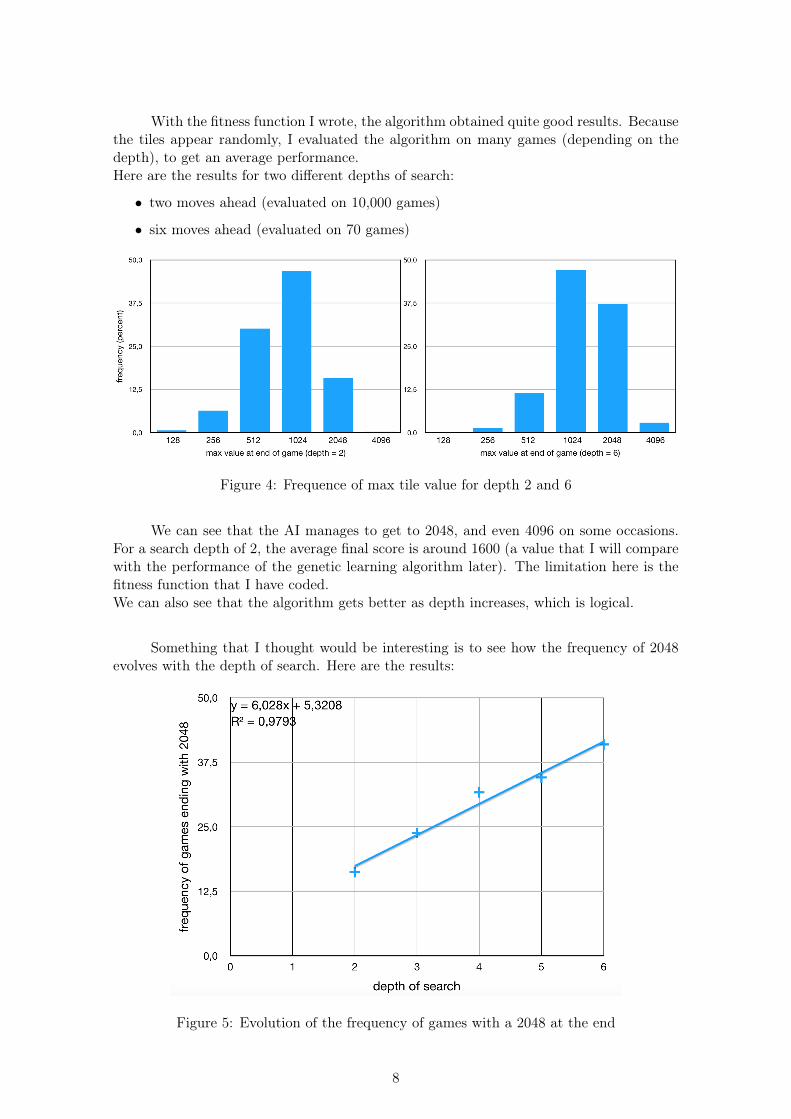
Something that I thought would be interesting is to see how the frequency of 2048evolves with the depth of search. Here are the results:

Figure 5: Evolution of the frequency of games with a 2048 at the end

8

What is quite surprising is that the ’score’ seems almost linearly dependent to thedepth of search! I expected the benefit of going deeper to decline at some point, as I donot take in account the numbers appearing randomly after each move. It is possible thatthis phenomenon becomes noticeable when searching deeper than 6 moves, but I have nottested it yet.

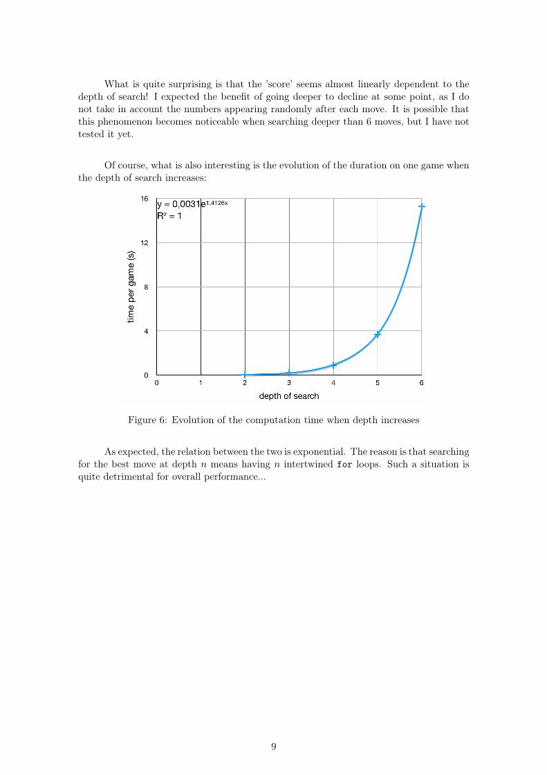
Of course, what is also interesting is the evolution of the duration on one game whenthe depth of search increases:

Figure 6: Evolution of the computation time when depth increases

As expected, the relation between the two is exponential. The reason is that searchingfor the best move at depth n means having n intertwined for loops. Such a situation isquite detrimental for overall performance...

9

4 The genetic learning algorithm

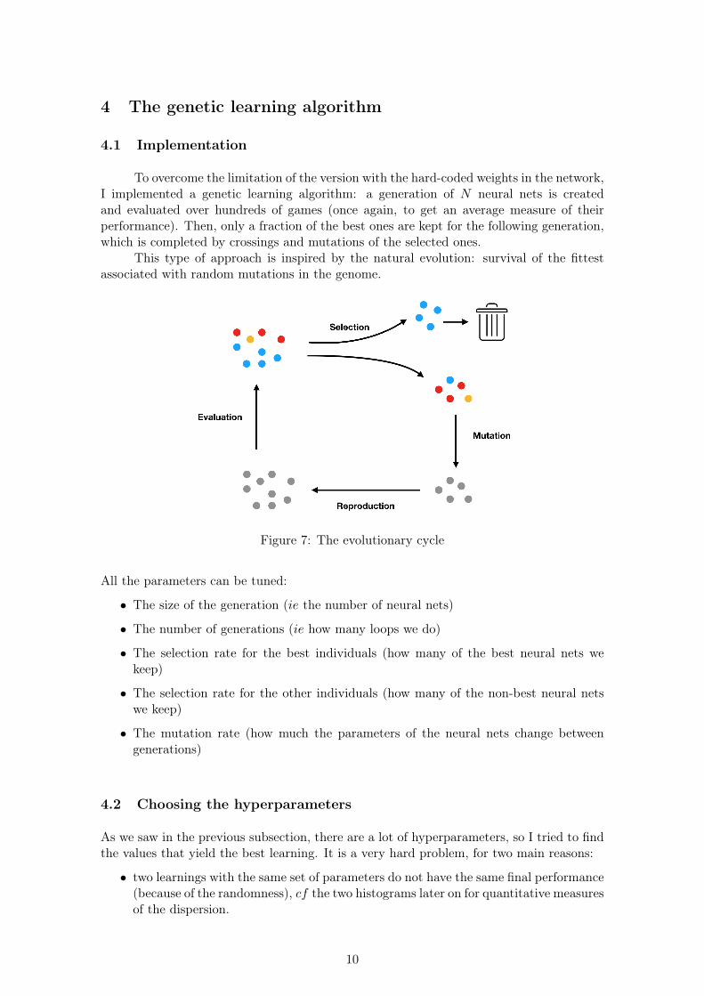
4.1 Implementation

To overcome the limitation of the version with the hard-coded weights in the network,I implemented a genetic learning algorithm: a generation of N neural nets is createdand evaluated over hundreds of games (once again, to get an average measure of theirperformance). Then, only a fraction of the best ones are kept for the following generation,which is completed by crossings and mutations of the selected ones.

This type of approach is inspired by the natural evolution: survival of the fittestassociated with random mutations in the genome.

Figure 7: The evolutionary cycle

All the parameters can be tuned:

• The size of the generation (ie the number of neural nets)

• The number of generations (ie how many loops we do)

• The selection rate for the best individuals (how many of the best neural nets wekeep)

• The selection rate for the other individuals (how many of the non-best neural netswe keep)

• The mutation rate (how much the parameters of the neural nets change betweengenerations)

4.2 Choosing the hyperparameters

As we saw in the previous subsection, there are a lot of hyperparameters, so I tried to findthe values that yield the best learning. It is a very hard problem, for two main reasons:

• two learnings with the same set of parameters do not have the same final performance(because of the randomness), cf the two histograms later on for quantitative measuresof the dispersion.

10

• the influences of the parameters on the learning are not independent. For instance,the optimal selection rate may depend on the value of the mutation rate.

As such, I decided to find the optimal parameters in the following order:

• size of a generation

• selection rate for best individuals

• selection rate for other individuals

• mutation rate

• number of generations

4.2.1 Size of a generation

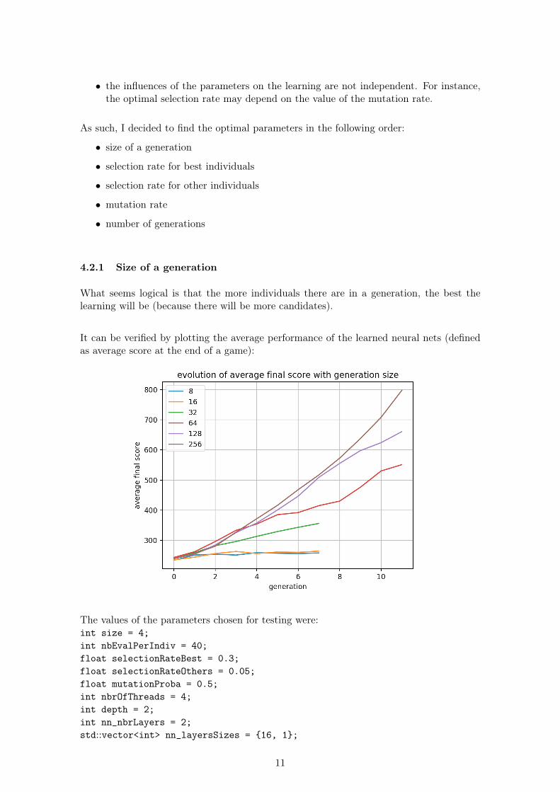
What seems logical is that the more individuals there are in a generation, the best thelearning will be (because there will be more candidates).

It can be verified by plotting the average performance of the learned neural nets (definedas average score at the end of a game):

The values of the parameters chosen for testing were:int size = 4;int nbEvalPerIndiv = 40;float selectionRateBest = 0.3;float selectionRateOthers = 0.05;float mutationProba = 0.5;int nbrOfThreads = 4;int depth = 2;int nn_nbrLayers = 2;std::vector<int> nn_layersSizes = {16, 1};

11

std::vector<int> nn_nonLinearities = {0};

Our intuition is verified, that is why for future tests I chose a generation size of256 (I could have gone for more, but it was already very long...).

4.2.2 Selection rate for best individuals

The selection rate of the best individuals is trickier to tune in the way its effect on finalscore is strongly influenced by the selection rate of the other (ie non best) individuals.

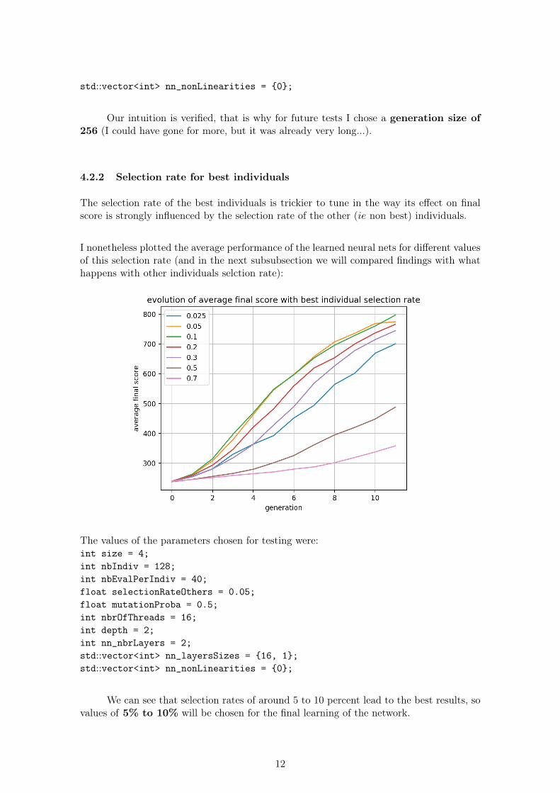
I nonetheless plotted the average performance of the learned neural nets for different valuesof this selection rate (and in the next subsubsection we will compared findings with whathappens with other individuals selction rate):

The values of the parameters chosen for testing were:int size = 4;int nbIndiv = 128;int nbEvalPerIndiv = 40;float selectionRateOthers = 0.05;float mutationProba = 0.5;int nbrOfThreads = 16;int depth = 2;int nn_nbrLayers = 2;std::vector<int> nn_layersSizes = {16, 1};std::vector<int> nn_nonLinearities = {0};

We can see that selection rates of around 5 to 10 percent lead to the best results, sovalues of 5% to 10% will be chosen for the final learning of the network.

12

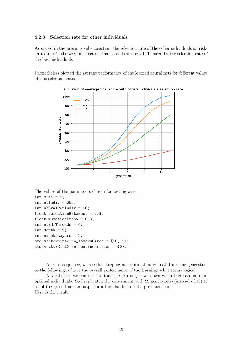
4.2.3 Selection rate for other individuals

As stated in the previous subsubsection, the selection rate of the other individuals is trick-ier to tune in the way its effect on final score is strongly influenced by the selection rate ofthe best individuals.

I nonetheless plotted the average performance of the learned neural nets for different valuesof this selection rate:

The values of the parameters chosen for testing were:int size = 4;int nbIndiv = 256;int nbEvalPerIndiv = 40;float selectionRateBest = 0.3;float mutationProba = 0.3;int nbrOfThreads = 4;int depth = 2;int nn_nbrLayers = 2;std::vector<int> nn_layersSizes = {16, 1};std::vector<int> nn_nonLinearities = {0};

As a consequence, we see that keeping non-optimal individuals from one generationto the following reduces the overall performance of the learning, what seems logical.

Nevertheless, we can observe that the learning slows down when there are no non-optimal individuals. So I replicated the experiment with 22 generations (instead of 12) tosee if the green line can outperform the blue line on the previous chart.Here is the result:

13

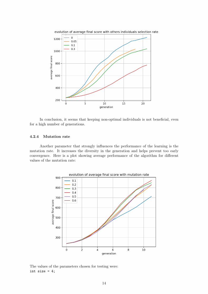
In conclusion, it seems that keeping non-optimal individuals is not beneficial, evenfor a high number of generations.

4.2.4 Mutation rate

Another parameter that strongly influences the performance of the learning is themutation rate. It increases the diversity in the generation and helps prevent too earlyconvergence. Here is a plot showing average performance of the algorithm for differentvalues of the mutation rate:

The values of the parameters chosen for testing were:int size = 4;

14

int nbIndiv = 256;int nbEvalPerIndiv = 40;float selectionRateBest = 0.3;float selectionRateOthers = 0.1;int nbrOfThreads = 4;int depth = 2;int nn_nbrLayers = 2;std::vector<int> nn_layersSizes = {16, 1};std::vector<int> nn_nonLinearities = {0};

We can see that the mutation rate does not have a strong influence on the averagefinal score. Nevertheless, a mutation rate around 30%-40% seems to be the optimal value.

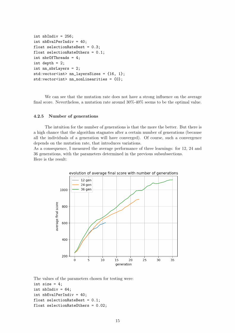
4.2.5 Number of generations

The intuition for the number of generations is that the more the better. But there isa high chance that the algorithm stagnates after a certain number of generations (becauseall the individuals of a generation will have converged). Of course, such a convergencedepends on the mutation rate, that introduces variations.As a consequence, I measured the average performance of three learnings: for 12, 24 and36 generations, with the parameters determined in the previous subsubsections.Here is the result:

The values of the parameters chosen for testing were:int size = 4;int nbIndiv = 64;int nbEvalPerIndiv = 40;float selectionRateBest = 0.1;float selectionRateOthers = 0.02;

15

float mutationProba = 0.4;int nbrOfThreads = 4;int depth = 2;int nn_nbrLayers = 2;std::vector<int> nn_layersSizes = {16, 1};std::vector<int> nn_nonLinearities = {0};

As a consequence, it seems that the algorithm does not have a tendency to stagnate whenthe number of generations increases (at least for these values of the parameters). So for’real’ tranings I will try to have a high number of generations.

4.2.6 Conclusion of the choice of hyperparameters

The way I tested for the optimal values of the hyperparameters is not ideal (because ofthe inter-dependencies), but I tried to be as rigorous as possible.And testing for these parameters required playing around 16 million games!

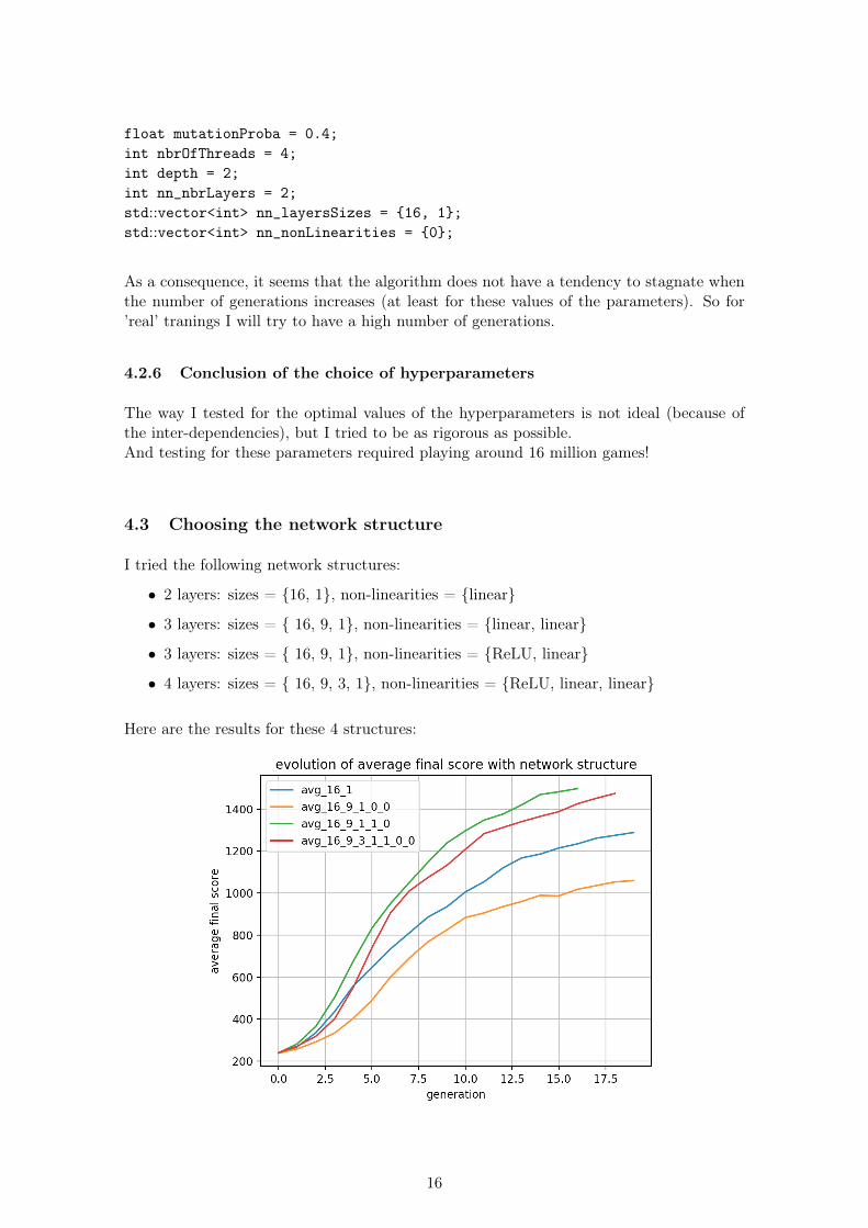
4.3 Choosing the network structure

I tried the following network structures:

• 2 layers: sizes = {16, 1}, non-linearities = {linear}

• 3 layers: sizes = { 16, 9, 1}, non-linearities = {linear, linear}

• 3 layers: sizes = { 16, 9, 1}, non-linearities = {ReLU, linear}

• 4 layers: sizes = { 16, 9, 3, 1}, non-linearities = {ReLU, linear, linear}

Here are the results for these 4 structures:

16

As a consequence, I will use the structure with 3 layers with : sizes = { 16, 9, 1} andnon-linearities = {ReLU, linear}

4.4 A note on the randomness

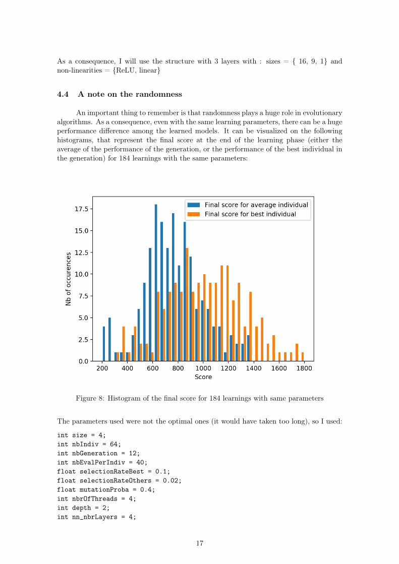
An important thing to remember is that randomness plays a huge role in evolutionaryalgorithms. As a consequence, even with the same learning parameters, there can be a hugeperformance difference among the learned models. It can be visualized on the followinghistograms, that represent the final score at the end of the learning phase (either theaverage of the performance of the generation, or the performance of the best individual inthe generation) for 184 learnings with the same parameters:

Figure 8: Histogram of the final score for 184 learnings with same parameters

The parameters used were not the optimal ones (it would have taken too long), so I used:

int size = 4;int nbIndiv = 64;int nbGeneration = 12;int nbEvalPerIndiv = 40;float selectionRateBest = 0.1;float selectionRateOthers = 0.02;float mutationProba = 0.4;int nbrOfThreads = 4;int depth = 2;int nn_nbrLayers = 4;

17

std::vector<int> nn_layersSizes = {16, 9, 3, 1};std::vector<int> nn_nonLinearities = {1, 0, 0};

4.5 Results for the chosen structure

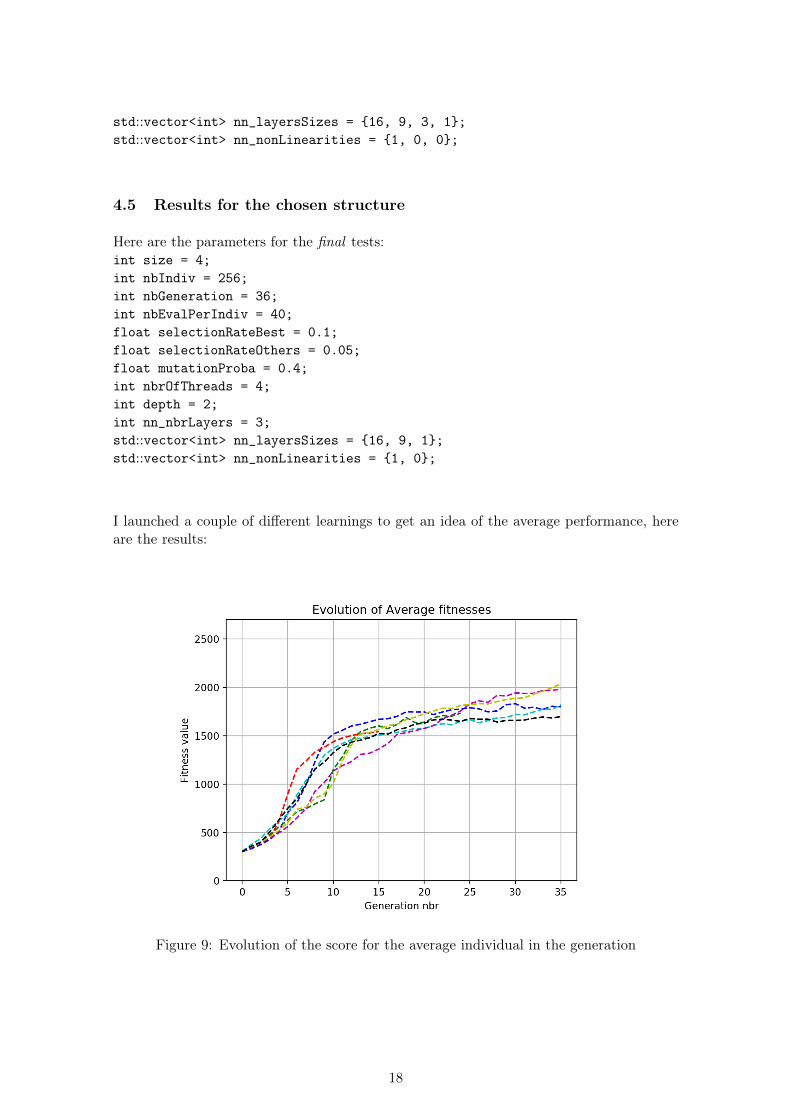
Here are the parameters for the final tests:int size = 4;int nbIndiv = 256;int nbGeneration = 36;int nbEvalPerIndiv = 40;float selectionRateBest = 0.1;float selectionRateOthers = 0.05;float mutationProba = 0.4;int nbrOfThreads = 4;int depth = 2;int nn_nbrLayers = 3;std::vector<int> nn_layersSizes = {16, 9, 1};std::vector<int> nn_nonLinearities = {1, 0};

I launched a couple of different learnings to get an idea of the average performance, hereare the results:

Figure 9: Evolution of the score for the average individual in the generation

18

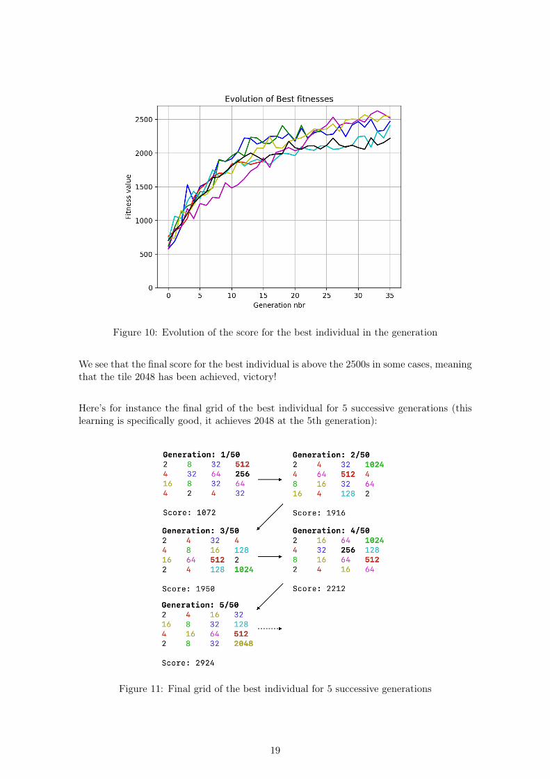
Figure 10: Evolution of the score for the best individual in the generation

We see that the final score for the best individual is above the 2500s in some cases, meaningthat the tile 2048 has been achieved, victory!

Here’s for instance the final grid of the best individual for 5 successive generations (thislearning is specifically good, it achieves 2048 at the 5th generation):

Figure 11: Final grid of the best individual for 5 successive generations

19

4.6 Conclusion of the neural net approach

In conclusion, the neural net approach, coupled with genetic evolution is a good wayto learn how to play 2048: it improves the final score by a factor of 9 compared to a randomapproach.

What is challenging here is that the random approach (ie making random moves) isnot that bad, which means that the good individuals do not stand out of the crowd by abig margin. Moreover, it is a computationally-intensive method.

20

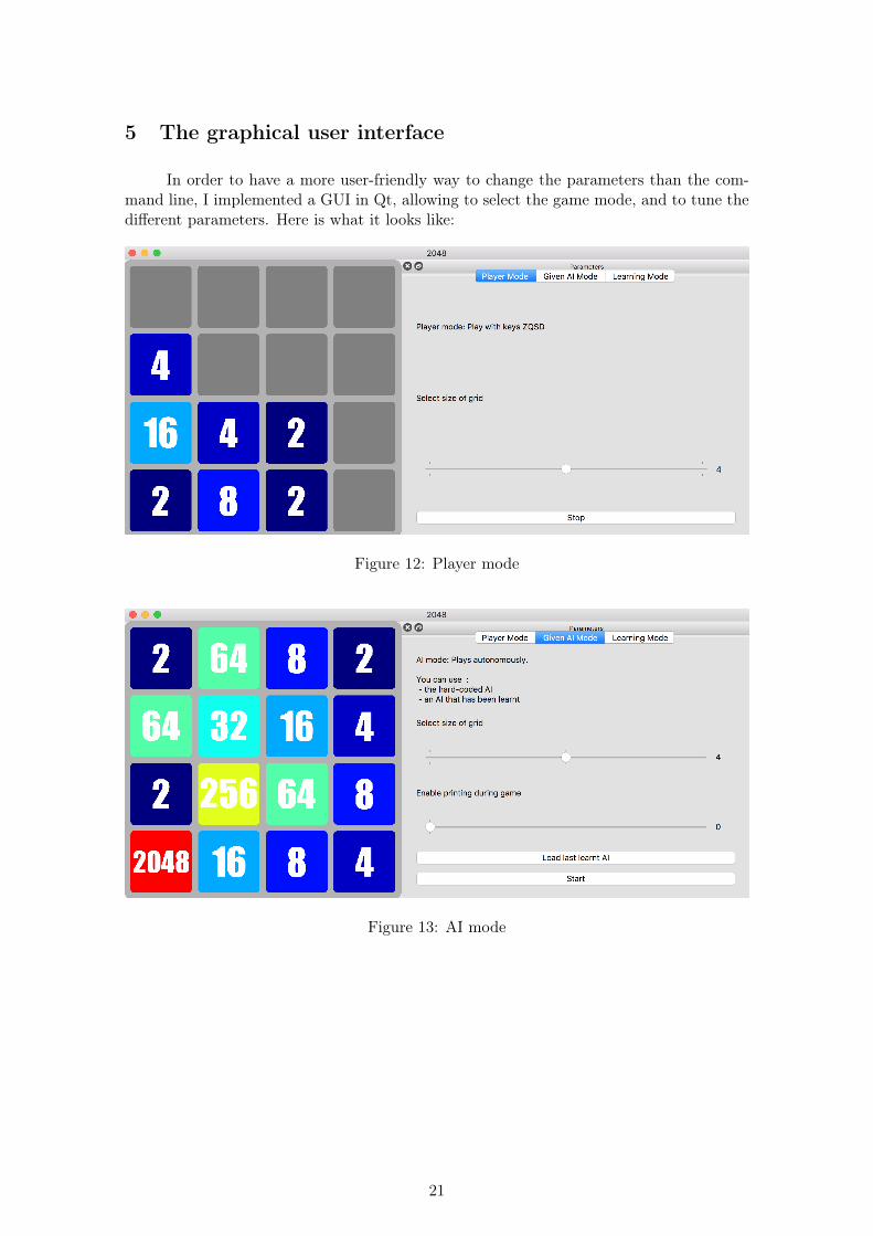
5 The graphical user interface

In order to have a more user-friendly way to change the parameters than the com-mand line, I implemented a GUI in Qt, allowing to select the game mode, and to tune thedifferent parameters. Here is what it looks like:

Figure 12: Player mode

Figure 13: AI mode

21

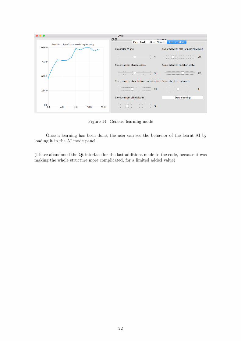
Figure 14: Genetic learning mode

Once a learning has been done, the user can see the behavior of the learnt AI byloading it in the AI mode panel.

(I have abandoned the Qt interface for the last additions made to the code, because it wasmaking the whole structure more complicated, for a limited added value)

22

Conclusion and future improvements

In conclusion, the hard-coded neural net works better than what I expected byachieving 2048 from time to time and even 4096! When it comes to the genetic version,we can see that some learning happens: there is a factor of 9 between the performancebefore and after the training (and the learnt technique is better than the heuristic I havehardcoded!).

What is really interesting is that with more computation power, the performancecan still improve! For many of the hyperparameters, there seem to be no bound on howthey can improve the learning:

• doubling the number of individuals leads to linear improvement in the final score

• increasing the number of generations does not seem to cause a decrease in the learning(it slows down but keeps improving)

• increasing the depth of search leads to linear improvement in the final score

In terms of speed, the hard-coded AI reaches 2048 in 0.08s on my 2.4 GHz IntelCore i5 Mac (roughly 4500 times quicker than when I play!). As a comparison, a Pythonprototype I wrote at the beginning of the project was running 100 times slower.

In terms of improvements, here are the different aspects I would like to work on:

• Allow multi-threading for the hard-coded fitness function mode.

• Change the reproduction phase in the learning mode (make it less brutal than aver-aging the weights grid of the two parents).

• Improving my neural net library to have more knobs available.

• Try Q-Learning (a variation of evolutionary algorithms)

Thanks for reading!

23