Batching and Scheduling with Tardiness Penalties

MISTA 2009

BATCHING AND SCHEDULING WITH TARDINESS

PENALTIES

Oncu Hazir · Safia Kedad-Sidhoum ·

Philippe Chretienne

Abstract In this paper, we address batching and scheduling a single production

system minimizing tardiness penalties. We define the optimal batching problem and

scheduling problem, which is an integrated lot-splitting and scheduling problem. We

examine the structural properties of the optimal solution and present some theoretical

results. Using these results, an efficient dynamic programming algorithm is proposed.

1 Introduction

Production planning and control decisions are traditionally categorized into three lev-

els: strategic, tactical and operational. In this research, we focus on the tactical and

operational levels, and concentrate on lot-sizing, lot-streaming and scheduling prob-

lems. Lot-sizing, which is a tactical decision, identifies when and how much to produce

so that the total cost is minimized. On the other hand, lot-streaming deals with split-

ting the production into batches with respect to the quantities of product planned.

It is usually used for planning demands in multi-stage production systems so that the

successive operations could overlap. By this way, lead times and work in process (WIP)

inventories -control of which is crucial in just in time (JIT) production- could be re-

duced. There exists a large number of studies on lot-streaming and we refer the readers

to the paper of [2] for a comprehensive survey. In addition to streaming, integration of a

pegging and a scheduling phase that assigns lots to demands and sets the starting time

of the lots respectively minimizing time or cost based criterion is valuable to generate

globally optimal production plans.

Integrated lot-sizing, streaming and scheduling problems has been a research topic

with practical implications, [3],[4]. In the scheduling literature, batch scheduling mod-

els, especially with set up times and costs, have been investigated by various researchers

(see [1] for a comprehensive review). In these models, either job processing times are

usually assumed to be fixed; or in some cases they are assumed to be controllable. When

lot-streaming is incorporated, total processing time is fixed but early completion of the

Oncu Hazir, Safia Kedad Sidhoum, Philippe ChretienneLaboratoire d’Informatique de Paris 6, 104 Avenue du President Kennedy, 75016 Paris, France.E-mail: [email protected], [email protected], [email protected]

Multidisciplinary International Conference on Scheduling : Theory and Applications (MISTA 2009) 10-12 August 2009, Dublin, Ireland

291

lots is possible. Potts and Van Wassenhove [5] make a review of integrated models

that combine batching and lot-sizing decisions with scheduling. On the other hand,

Selvarajah and Steiner [7] address the batching scheduling problem in a supply chain

from the supplier’s point of view. The aim is find the number of batches, batch sizes

and the optimal schedule, while minimizing the total inventory holding and delivery

cost.

Recently, Robert [6] combined lot-streaming and pegging, which addresses the

transfer of materials between stocks and users, and used linear programming soft-

ware to solve the derived models. In addition, she proposed a dynamic programming

model that minimizes the sum of production costs and tardiness costs.

The problem could be defined as follows: We consider a single production system

which can handle at most one customer order at a time and for which the nominal

production rate is the same for all orders. Demand is deterministic and all orders

are ready to be processed at time zero. We have K customer orders to satisfy. Each

customer order k demands rk units to be delivered at the due date dk. If the order k

is delivered after dk, a penalty βk, is paid. Two pegging conditions are considered: in

mono-pegging, it is required that each customer order is met from a single batch, on

the contrary in multi-pegging, orders could be satisfied from different batches. Batch

availability is assumed, meaning that a product could not be released before its batch

is completely processed. There exists lower and upper bound constraints, b and B, on

the size of batch i. The starting and completion time of batch i will be denoted by Si

and Ci, respectively.

The cost of producing qki units of order k in batch i is βkqk

i T ki where T k

i = (Ci −

dk)+ is the tardiness of batch i with respect to due date dk. The objective function is

a quadratic function and it penalizes tardy deliveries. Then the problem is to find a

production schedule with a minimum cost.

A production schedule Ψ could be defined as, (N, q, S) where N represents the total

number of batches, and q defines the batch production variables with elements, qki for

i = 1, ..., N and k = 1, ..., K, and S defines batch starting times. A feasible schedule

must

(1) satisfy the batch size constraints:

b ≤PK

k=1 qki ≤ B for i = 1, ..., N , and

(2) ensure that the time intervalsh

Si, Si +PK

k=1 qki

i

do not overlap, and

(3) ensure that all orders are met:PN

i=1 qki = rk for k = 1, ..., K.

The objective is to find a feasible schedule that minimizes the total cost:

f(Ψ∗) = Minn

PNi=1

PKk=1 βkqk

i (Ci − dk)+o

In the sequel, we address a practically relevant special case denoted with (P),

multi-pegging with demand independent weights,i.e. βk = β for all k = 1, ..., K. This

case represents the case where customers are equivalently important. Problem (P),

which we study in this resarch, encourages early deliveries and addresses scheduling the

production systems in which partial delivery of orders are possible. Partial deliveries are

widely encountered in industry because it prevents customer stock outs and improves

customer service. Our model is applicable to model bottleneck stations and the results

presented in this paper would serve as a basis to model more complicated production

systems.

The organization of the paper is as follows: We first present some structural prop-

erties of an optimal schedule, then in order to solve (P), we propose a dynamic pro-


292

gramming based model that uses these properties. Finally, we discuss some possible

extensions and future issues.

2 Structural Properties of an Optimal Schedule

Recently, Robert [6] investigated this problem (P) and defined the following properties:

Property 1. Processing the batches in a left justified single block without idle

times is dominant.

Property 2. In multi-pegging with unitary weights, earliest due date (EDD) sched-

ules are dominant.

Property 3. In multi-pegging, the batches with sizes in between b and 2b − 1 are

dominant when only tardiness cost is minimized.

In addition to the properties defined above, we present some novel structural prop-

erties of the optimal solution. Let us first introduce the following definitions:

A batch i is called tardy if it only consists of tardy units, i.e. Ci > dk for all

k = 1, ..., K such that qki > 0, and called early if it only consists of early units, i.e.

Ci < dk such that qki > 0 and on time if Ci = dk such that qk

i > 0. In addition, we

call a batch that processes only a single order uniform. We assume that the nominal

unit production time is one unit time for any item so that the production quantity,

qki , also refers to the time required to process the customer order k in batch i. From

now on, using property 2, without loss of generality (w.l.o.g.), we will number the

customer orders according to the EDD rule and schedule accordingly, i.e. k < l implies

that dk ≤ dl. Now we present some novel structural properties of an optimal schedule.

Lemmas 1-4 address the batch sizing of the tardy batches.

2.1 Optimal Sizing of Tardy Batches

Lemma 1. There exists an optimal schedule where the consecutive tardy batches are

ordered in non-decreasing batch size (SPT order).

Proof: First we will consider rescheduling two tardy consecutive batches. Let the

optimal schedule Ψ have two consecutive tardy batches, namely batches i and j with

i < j. Due to property 1, these two batches should be adjacent. Let us assume the

following contradictory case, qi > qj :

j

ji

i

Ci

l

Ci

Cj

l

Cjdk

Fig. 1 Illustration of Lemma 1


293

A new schedule Ψ ’ could be generated by transferring the last unit of batch i

(denote this unit by [l]) to batch j. As b ≤ qj < qi ≤ B in schedule Ψ , feasibility

will be maintained in schedule Ψ ’, i.e. either b < q′j = qj + 1 ≤ q′i = qi − 1 < B or

b ≤ q′i = qj ≤ q′j = qi ≤ B. We illustrate both of the schedules in Figure 1. Each

rounded rectangle represents a batch in the figure.

As a result of this operation, unit [l] will complete later by an amount of qj whereas

all the remaining units in batch i will complete earlier by an amount of 1 time unit.

The cost difference could be formulated as:

f(Ψ) − f(Ψ ′) = β`

qi − 1 − qj

´

.

As f(Ψ) − f(Ψ ′) ≥ 0, the transfer of the units until either qi ≤ qj or any order k in

batch i becomes on time would not increase the costs.

On the other hand, for consecutive batches including more than two batches, the

above mentioned transferring procedure could be reiterated. As a result, by a series of

transfer operations among the adjacent batches, any schedule Ψ that includes non-SPT

consecutive tardy batches could be converted to a schedule that satisfies the lemma

(SPT order) without increasing the cost Ψ . �

Lemma 2. There exists an optimal schedule where the absolute difference between

the sizes of any two tardy and uniform batches which process the same order is at most

1.

Proof: Let the optimal schedule Ψ have tardy uniform batches which process the

customer order k. We know that this order is processed consecutively without any

preemption (no idle time and no other order in between). As all these tardy batches

would be consecutive, conditions of Lemma 1 applies as well. Among these batches, let

us consider any two, namely batches i and j with i < j. Owing to Lemma 1, we can

assume that qi ≤ qj w.l.o.g. In addition let us assume the following contradictory case

for schedule Ψ , qi + 1 < qj :

We can generate a new schedule Ψ ′ by transferring one unit of batch j( denote this

unit with [l]) to the batch i. Consequently, all the units in batches prior to batch j will

complete later by an amount of 1 time unit, whereas unit [l], will be tardy in batch

i as well, because the units of the same order are tardy in batch i, but it completes

earlier by an amount ofPk=j

k=i+1 qk − 1 time unit. We illustrate both of the schedules

in Figure 2.

i l

Ci

j

Ci

i l j

dk

Cj

Cj

Fig. 2 Illustration of Lemma 2


294

As b ≤ qi < qi+1 < qj ≤ B in schedule Ψ , feasibility will be maintained in schedule

Ψ ′, i.e. b < q′i = qi + 1 ≤ q′j = qj − 1 < B. The cost difference would be:

f(Ψ) − f(Ψ ′) = β

0

@

k=jX

k=i+1

qk − 1 −

k=j−1X

k=i

qk

1

A = β`

qj − 1 − qi

´

> 0.

Since f(Ψ) − f(Ψ ′) > 0, the transfer of the units would be profitable until either

qj − 1 ≤ qi or the order k in batch i becomes on time. This contradicts the optimality

of schedule Ψ . �

Corollary 1: There exists an optimal schedule where the tardy batches that pro-

cess the same order have the following structure: qj − 1 ≤ qi ≤ qj for any i < j.

Proof: Due to property 1, all the tardy batches which process the same order are

consecutive. Using Lemma 1 and 2, the result follows. �

Using Corollary 1, we propose the following lemma to construct the optimal sched-

ule for tardy orders. In the sequel, we will denote the minimum and maximum number

of batches to process Q units by hmin = ⌈QB ⌉ and hmax = ⌊Q

b ⌋ respectively. Further-

more, in the following lemmas, we assume that ⌈QB ⌉ ≤ ⌊Q

b ⌋, otherwise, the problem is

infeasible [6].

Lemma 3. Given any time window T = [t, t′], if only Q units from a single customer

order k are to be processed with h batches such that hmin ≤ h ≤ hmax and dk ≤ t,

there exists an optimal schedule in which, the first h1 = ⌈Qh⌉ ∗ h−Q batches have size

m1 = ⌈Qh ⌉ − 1 and the remaining h2 = h − h1 batches have size m2 = ⌈Q

h ⌉.

Proof: As dk ≤ t and a single order is processed, all the batches in T would

be tardy and uniform and there exists no idle time between the batches. Since the

conditions of Lemmas 1 and 2 is satisfied, there exists an optimal schedule Ψ that has

the structure given in Corollary 1.

Considering Corollary 1, let us schedule the Q′ = Q − h2 units in the interval

T = [t, t′] first. In this case, all the h batches should have equal size m1 = ⌈Qh⌉ − 1

and b ≤ m1 < B. The remaining h2 extra units should be processed within the last h2

batches, one unit in each batch. Otherwise, the conditions of Lemmas 1 and 2 would

be violated. �.

We illustrate the structure with the following simple example:

Example 1. Given the following data dk = 10, Q = 17, T = [12, 30], b = 3, B = 5

and h = 4, Lemma 3 results in the structure h1 = 3, h2 = 1, m1 = 4, m2 = 5 or 4, 4, 4,

5. Formally, starting from time 12, the first 3 batches have size of 4 whereas the last

batch will have a size of 5.

Lemma 4. Given any time window T = [t, t′], if only Q units from a single customer

order k is to be processed within T = [t, t′] and dk ≤ t, there exists an optimal schedule

with hmax = ⌊Qb⌋ batches in T .

Proof:

Let the optimal schedule Ψ have Nb < hmax batches and satisfies the conditions of

the lemma. As all these batches would be tardy and a single customer order k is to be

processed, conditions of Lemmas 1 and 2 apply. Let us integrate hmax − Nb dummy

batches with size 0 at the end of schedule Ψ . Starting from the last batch, the transfer of

the units as explained in the proofs of Lemmas 1 and 2, and reiterating until conditions

of Corollary 1 are satisfied results in a schedule with hmax batches without increasing

the cost. Feasibility will be satisfied at the end, because according to Lemma 3, there

will be h1 = ⌈ Qhmax

⌉ ∗ hmax − Q batches with size m1 = ⌈ Qhmax

⌉ − 1 and h2 = h − h1


295

batches of size m2 = ⌈ Qhmax

⌉ at the end. Using the definition of hmax, if h1 > 0, b <Q

hmaxand b ≤ m1 < m2 ≤ B. Therefore, schedule Ψ could be converted to a schedule

with hmax batches without increasing the cost. �.

Example 2. Consider the previous example, but without fixing the number of

batches. In this case, according to Lemma 4, there exists an optimal schedule with

hmax = 5 batches and the optimal structure would be 3, 3, 3, 4, 4.

2.2 Equivalence Properties of the Tardiness Cost

We will refer to the following Lemma in finding out the cost of tardy batches:

Lemma 5. The problem (P1) to find the optimal schedule to process Q units of any

customer order in time window [t, t + Q] such that t < d and the first batch completes

after due date d is equivalent to the problem (P2) to optimally schedule Q units in

time window [d, d + Q] so that the first batch contains at least w = d − t units.

Proof: We denote cost functions of the problems P1 and P2 with f1, f2 and define

w = d − t, and ϑ = Max {b, w}. Let T (Q) defines the optimal cost of processing Q

units of a product in time window with length Q whose left hand is the deadline, i.e

window [d, d + Q], of the product.

On the other hand, if Q units start processing at time d + u, then the optimal cost

could be reformulated as βQu+T (Q). Using this property and denoting the size of the

first batch with x, then for each problem, we have:

f1(Q) = Minϑ≤x≤B{β [x(x − w) + (Q − x)(x − w)] + T (Q − x)}= Minϑ≤x≤B{βQ(x − w) + T (Q − x)}, where x is the size of the first batch;

f2(Q) = Minϑ≤x≤B{βh

x2 + x(Q − x)i

+ T (Q − x)}

= Minϑ≤x≤B{βQx + T (Q − x)}.As Q and w are given, P1 and P2 are equivalent. �.

Corollary 2: The problem to find the optimal schedule to process Q units product

in time window [t, t + Q] where d− b ≤ t ≤ d is equivalent to the problem to optimally

schedule Q units in time window [d, d + Q].

Proof: As w = d−t < b, then the first batch always completes after d and the result

follows from Lemma 5. �.

Note that we could use Lemma 3 to formulate T (Q) as:

T (Q) = β[Ph1

i=1 im21 +

Phi=h1+1(h1m1 + (i − h1)m2) ∗ m2] if ⌈Q

B ⌉ ≤ ⌊Qb ⌋. Otherwise

there is no feasible solution and a “big“ cost value is assigned.

In what follows, to solve the problem P, we propose a dynamic programming model

that uses all the properties defined above.

3 A Dynamic Programming Based Solution Algorithm

We describe a forward dynamic programming model has K stages that correspond to

the customer orders. In an optimal production plan, some of the orders could share

the same batch and because of the EDD rule, these batches could be either the first or

the last batch of the order. The intermediate batches process units only from a single

order hence they are uniform. We decompose each stage k and model the problem as

an optimization problem to determine the size of a single shared batch, which contains

units from order k + 1, and the sizes of intermediate uniform batches that process


296

units of order k. Let the variable xk+1 denote the number of units order k + 1 and

forthcoming orders processed within the same batch with units of order k. For any

order k = 1, ..., K, if b ≤ rk + xk+1, then units of order k could be processed in

multiple batches. In this case, the decision variables xk and yk represent the number

of units of order k to be processed within the same batch with units from the orders

k − 1 and k + 1, respectively. This case and the corresponding decision variables are

illustrated in Figure 3. From now on, we will denote cumulative orders shortly with R,

i.e. Rk =Pk

i=1 ri.

xkxk yk

Orders 1, 2, ..., k − 1 Orders k + 1, k + 2...

Rk−1 Rk

...... x

Fig. 3 Illustration of the Decision Variables

In the figure each rounded rectangle and color represent a batch and a customer

order, respectively. For feasibility, we require b ≤ yk + xk+1 ≤ B for k = 1, ..., K. An

upper bound would be UB = Min {2b − 1, B}, hence b ≤ yk + xk+1 ≤ UB. If the size

of the batch is larger than 2b, the batch could be split without increasing the costs of

the schedule.

On the other hand, when rk +xk+1 < b, lot-splitting is not feasible for order k and

the shared batch includes units from order k−1 as well. In this case, the units of order

k are all early, all on time or all tardy. Let hk(xk+1) denote the minimum total cost of

processing the first k orders given that the final batch of order k processes xk+1 units

of order k + 1 and forthcoming orders. Therefore, the optimal cost will be referred as

hn(0). We propose the following recursive model:

hk(xk+1) =

8

>

<

>

:

Minxk,yk{gk(xk, yk, xk+1) + hk−1(xk)} b ≤ rk + xk+1

βrk(Rk + xk+1 − dk) + hk−1(xk+1 + rk) rk + xk+1 < b, dk < Rk + xk+1

hk−1(xk+1 + rk) rk + xk+1 < b, dk ≥ Rk + xk+1

Note that gk(.) is defined for the case b ≤ rk + xk+1 and refers to the total cost of

units of order k. We will consider the following four cases to define gk(.). In these cases,

yk ≤ UB and xk ≤ UB for all k = 1, ..., K. In addition, we remind the assumption

that the nominal unit production time is one unit time for any item and Tk(Q) is the

optimal cost of processing Q units of customer order k by starting at the due date dk.

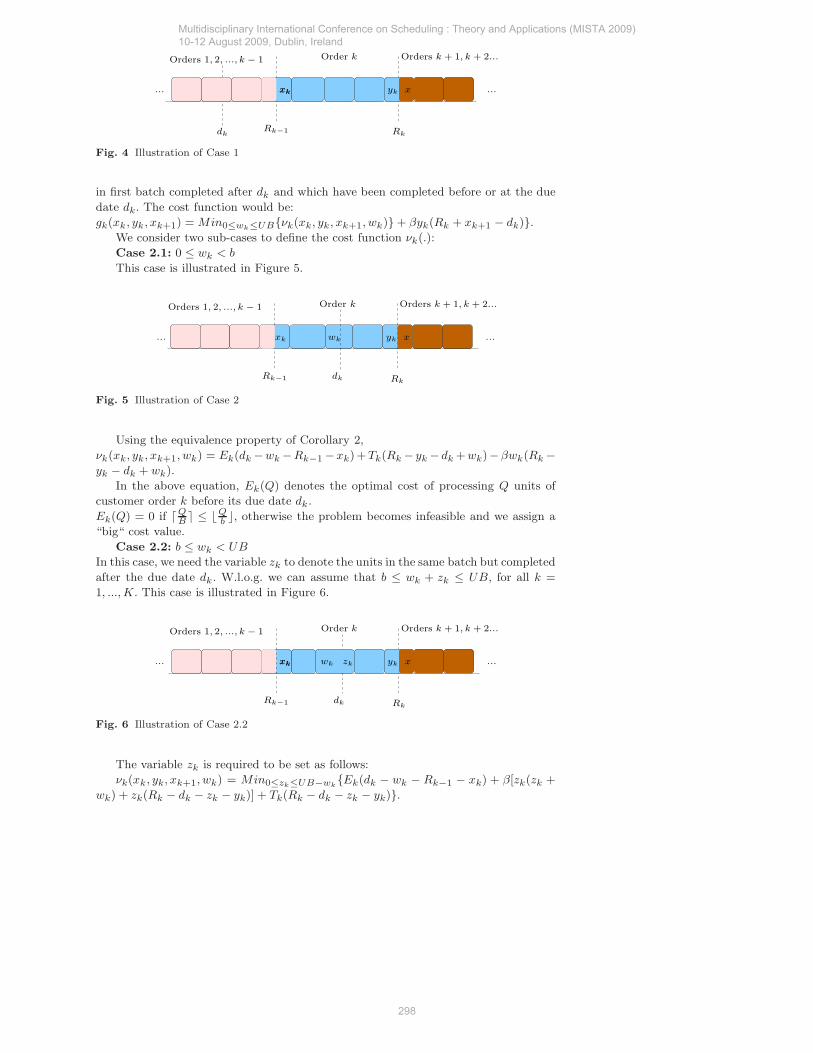
Case 1: If dk < Rk−1 +xk then, all the units of order k would be tardy. This case

is illustrated in Figure 4.

Using the equivalence property of Corollary 2,

gk(xk, yk, xk+1) = β[xk(Rk−1 + xk − dk) + (rk − xk − yk)(Rk−1 + xk − dk)]+ Tk(rk −

xk − yk) + βyk(Rk + xk+1 − dk).

= β(Rk−1 + xk − dk)(rk − yk) + Tk(rk − xk − yk) + βyk(Rk + xk+1 − dk).

Case 2: If Rk−1 + xk ≤ dk ≤ Rk − yk, then some of the intermediate batches

could be early, some on time and some could be tardy. To differentiate these, we need

the decision variable, wk. The variable wk denotes the units of the order k processed


297

xkxk yk

Orders 1, 2, ..., k − 1 Order k Orders k + 1, k + 2...

dkRk−1 Rk

...... x

Fig. 4 Illustration of Case 1

in first batch completed after dk and which have been completed before or at the due

date dk. The cost function would be:

gk(xk, yk, xk+1) = Min0≤wk≤UB{νk(xk, yk, xk+1, wk)} + βyk(Rk + xk+1 − dk)}.

We consider two sub-cases to define the cost function νk(.):

Case 2.1: 0 ≤ wk < b

This case is illustrated in Figure 5.

ykwk

Orders 1, 2, ..., k − 1 Order k Orders k + 1, k + 2...

Rk−1 dk Rk

...... xk x


Using the equivalence property of Corollary 2,

νk(xk, yk, xk+1, wk) = Ek(dk −wk −Rk−1 −xk)+Tk(Rk − yk − dk +wk)−βwk(Rk −yk − dk + wk).

In the above equation, Ek(Q) denotes the optimal cost of processing Q units of

customer order k before its due date dk.

Ek(Q) = 0 if ⌈QB ⌉ ≤ ⌊Q

b ⌋, otherwise the problem becomes infeasible and we assign a

“big“ cost value.

Case 2.2: b ≤ wk < UB

In this case, we need the variable zk to denote the units in the same batch but completed

after the due date dk. W.l.o.g. we can assume that b ≤ wk + zk ≤ UB, for all k =

1, ..., K. This case is illustrated in Figure 6.

xkxk ykwk zk

Orders 1, 2, ..., k − 1 Orders k + 1, k + 2...Order k

Rk−1 dk Rk

...... x

Fig. 6 Illustration of Case 2.2

The variable zk is required to be set as follows:

νk(xk, yk, xk+1, wk) = Min0≤zk≤UB−wk{Ek(dk − wk − Rk−1 − xk) + β[zk(zk +

wk) + zk(Rk − dk − zk − yk)] + Tk(Rk − dk − zk − yk)}.


298

= Min0≤zk≤UB−wk{Ek(dk−wk−Rk−1−xk)+β[zk(wk+Rk−dk−yk)]+Tk(Rk−

dk − zk − yk)}.

Case 3: If Rk − yk < dk < Rk + xk+1, then all the intermediate batches would be

early. This case is illustrated in Figure 7. The cost would be:

gk(xk, yk, xk+1) = Ek(rk − xk − yk) + βyk(Rk + xk+1 − dk).

xkxk yk

dk

Orders k + 1, k + 2...Order kOrders 1, 2, ..., k − 1

Rk−1 Rk

...... x


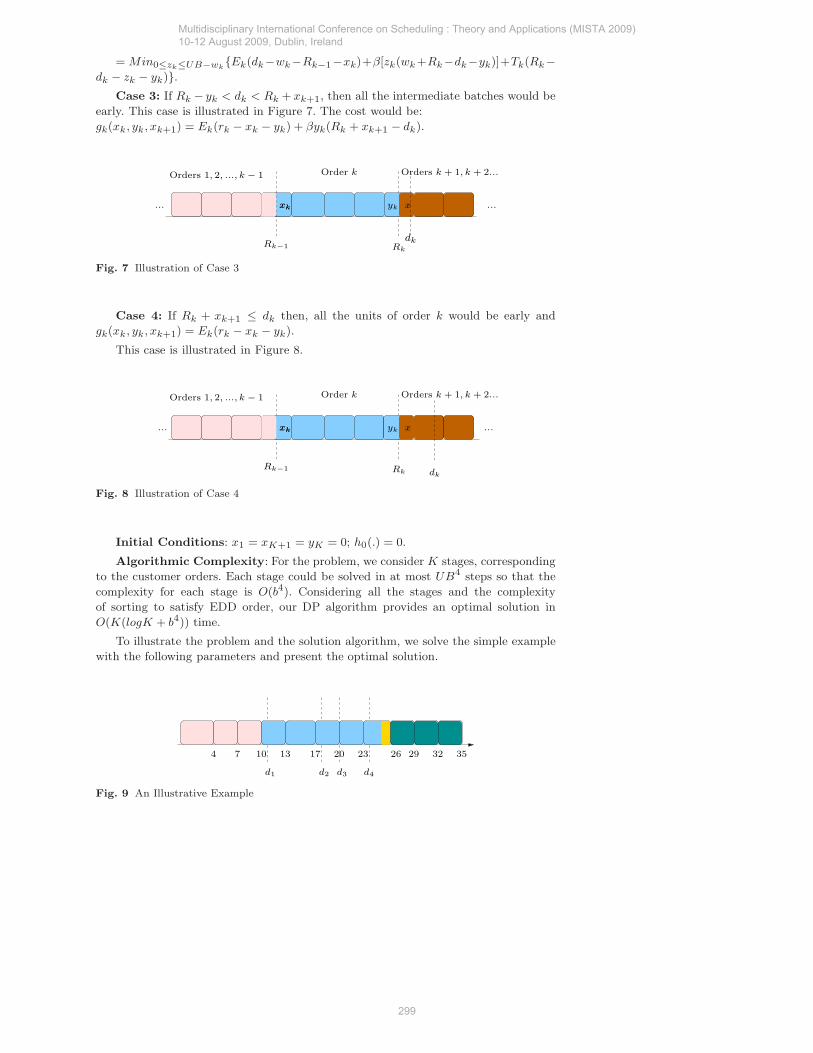
Case 4: If Rk + xk+1 ≤ dk then, all the units of order k would be early and

gk(xk, yk, xk+1) = Ek(rk − xk − yk).

This case is illustrated in Figure 8.

xkxk yk

Orders 1, 2, ..., k − 1 Order k

Rk−1 Rk dk

Orders k + 1, k + 2...

...... x


Initial Conditions: x1 = xK+1 = yK = 0; h0(.) = 0.

Algorithmic Complexity: For the problem, we consider K stages, corresponding

to the customer orders. Each stage could be solved in at most UB4 steps so that the

complexity for each stage is O(b4). Considering all the stages and the complexity

of sorting to satisfy EDD order, our DP algorithm provides an optimal solution in

O(K(logK + b4)) time.

To illustrate the problem and the solution algorithm, we solve the simple example

with the following parameters and present the optimal solution.

d1 d2

4 10 13 17

d3 d4

207 23 29 32 3526

Fig. 9 An Illustrative Example


299

An Illustrative Example: We consider scheduling four customer orders with

multi-pegging given the following data: K = 4; b = 3; B = 5; r1 = 10, r2 = 15, r3 =

1, r4 = 9; d1 = 11, d2 = 18, d3 = 20, d4 = 24.

The optimal schedule is illustrated in Figure 9 below. Each rounded rectangle

represents a customer order following the EDD rule and completion time of each batch

is illustrated in the time line below.

4 Conclusions

In this paper, we have investigated a production planning problem with tardiness penal-

ties for a single production system. In order to solve the problem, we have followed

an integrated lot-streaming and scheduling approach. We have examined the struc-

tural properties of the optimal solution, presented theoretical results, and developed a

dynamic programming algorithm that extensively makes use of these properties.

As a future extension of this research, we will incorporate the setup times and

costs and earliness penalties. Considering the real world requirements, integration of the

setup constraints is important. Furthermore, modeling both the earliness and tardiness

penalties addresses the JIT requirement of lower lead times and WIP, therefore is

practically relevant especially for just in time systems.

References

1. A. Allahverdi, C.T. Ng, T.C.E. Cheng, and M.Y. Kovalyov, A survey of scheduling prob-lems with setup times or costs, European Journal of Operational Research 187(3), 985-1032,(2008).

2. Chang J.H. and Chiu H.N., A comprehensive review of lot-streaming, International Journal

of Production Research 43 (8), 1515-1536 (2005).3. Dauzere-Peres S. and Lasserre J.B. On the importance of sequencing decisions in production

planning and scheduling. International Transactions in Operational Research, 9(6), 779-793,(2002).

4. Drexl A., and A Kimms, Lot sizing and scheduling: Survey and extensions, European Jour-

nal of Operational Research 99, 221-235 (1997).5. Potts C.N. and L.N. Van Wassenhove, Integrating scheduling with batching and lot-sizing:

A review of algorithms and complexity. Journal of the Operational Research Society 43395-406 (1992).

6. Robert A. Optimization des batches de production. PhD thesis, Universite Pierre et MarieCurie (Paris 6)(2007).

7. Selvarajah, E. and Steiner, G. Batch scheduling in a two-level supply chain: A focus on thesupplier. European Journal of Operational Research 173 226-240 (2006).


300

Batching and Scheduling with Tardiness Penalties

Documents

Transcript of Batching and Scheduling with Tardiness Penalties