Evaluating water stress controls on primary production in

biogeochemical and remote sensing based models

Qiaozhen Mu,1 Maosheng Zhao,1 Faith Ann Heinsch,1 Mingliang Liu,2 Hanqin Tian,2

and Steven W. Running1

Received 9 February 2006; revised 8 September 2006; accepted 6 October 2006; published 8 February 2007.

[1] Water stress is one of the most important limiting factors controlling terrestrialprimary production, and the performance of a primary production model is largelydetermined by its capacity to capture environmental water stress. The algorithm thatgenerates the global near-real-time MODIS GPP/NPP products (MOD17) uses VPD(vapor pressure deficit) alone to estimate the environmental water stress. This papercompares the water stress calculation in the MOD17 algorithm with results simulatedusing a process-based biogeochemical model (Biome-BGC) to evaluate the performanceof the water stress determined using the MOD17 algorithm. The investigation study areasinclude China and the conterminous United States because of the availability of dailymeteorological observation data. Our study shows that VPD alone can capture interannualvariability of the full water stress nearly over all the study areas. In wet regions, whereannual precipitation is greater than 400 mm/yr, the VPD-based water stress estimate inMOD17 is adequate to explain the magnitude and variability of water stress determinedfrom atmospheric VPD and soil water in Biome-BGC. In some dry regions, where soilwater is severely limiting, MOD17 underestimates water stress, overestimates GPP, andfails to capture the intraannual variability of water stress. The MOD17 algorithm shouldadd soil water stress to its calculations in these dry regions, thereby improving GPPestimates. Interannual variability in water stress is simpler to capture than the seasonality,but it is more difficult to capture this interannual variability in GPP. The MOD17algorithm captures interannual and intraannual variability of both the Biome-BGC-calculated water stress and GPP better in the conterminous United States than in thestrongly monsoon-controlled China.

Citation: Mu, Q., M. Zhao, F. A. Heinsch, M. Liu, H. Tian, and S. W. Running (2007), Evaluating water stress controls on primary

production in biogeochemical and remote sensing based models, J. Geophys. Res., 112, G01012, doi:10.1029/2006JG000179.

1. Introduction

[2] Water availability is the primary limiting factor forvegetation growth over 40% of the Earth’s vegetatedsurface, while an additional 33% is limited by cold temper-atures and frozen water, further limiting water availabilityfor plant growth [Nemani et al., 2003]. Vegetation respondsto water deficits in several ways [Waring and Running,1998]. Even mild soil water deficits begin to inhibit cellularexpansion, xylem water flow from roots to leaves, andphloem sugar transfer in the stems of growing plants. Lackof mobile water has similar impacts on reducing plant leafarea, transpiration, growth, and related ecosystem activity[Running and Kimball, 2005].

[3] Terrestrial net primary production (NPP), equal to thedifference between gross primary production (GPP) andautotrophic respiration (Ra), plays an important role in thecarbon balance of the biosphere. NPP is receiving increasedattention not only because it is related to the global carboncycle, but also because it is greatly influenced by theassociated effects of changing climate on the carbon cycle[Prentice et al., 2001]. Photosynthesis is the only process bywhich to assimilate CO2 from the atmosphere into terrestrialprimary production, and stomata are the major pathways fortransfer of trace gases between vegetation and the atmo-sphere. The stomatal conductance and photosynthetic as-similation rate are largely controlled by environmentalfactors such as irradiance, temperature, water availability,and nutrition [Wong et al., 1985a, 1985b, 1985c; Lange etal., 1987]. Therefore global terrestrial primary productionmodels incorporate these environmental factors to study theterrestrial carbon balance and vegetation dynamics under achanging climate [Cramer et al., 1999; Arora, 2002]. Plantwater deficits induce progressive leaf stomatal closure,reducing plant water loss via transpiration while also slow-

JOURNAL OF GEOPHYSICAL RESEARCH, VOL. 112, G01012, doi:10.1029/2006JG000179, 2007ClickHere

for

FullArticle

1Numerical Terradynamic Simulation Group, Department of Ecosystemand Conservation Sciences, University of Montana, Missoula, Montana,USA.

2School of Forestry and Wildlife Sciences, Auburn University, Auburn,Alabama, USA.

Copyright 2007 by the American Geophysical Union.0148-0227/07/2006JG000179$09.00

G01012 1 of 13

ing photosynthesis and canopy-atmosphere gas exchange.Sustained drought will produce early leaf senescence andshedding and may impact ecosystem leaf area for a numberof years [Running and Kimball, 2005]. During most of thegrowing season, when light and temperature are greatenough to maximize stomatal conductance, water limitationis the dominant climatic controller of stomatal conductance.There are different approaches to introducing water limi-tations on primary production in different models, and formost process-based ecosystem models, water limitations arecalculated for both the soil and the air [Churkina et al.,1999].[4] The Biome-BGC ecosystem model is a process-

based biogeochemical model, simulating ecosystem cyclesof carbon, water and nitrogen at regional and global scales[Running and Hunt, 1993; White et al., 2000; Thornton etal., 2002]. The water stress calculation in Biome-BGC isdetermined by the combined stresses from soil-leaf waterpotential (PSI) and the atmospheric water vapor pressuredeficit (VPD; details in section 2.1). The operationalMODIS (Moderate Resolution Imaging Spectroradiometer)Production Efficiency Model (MOD17) on the Terra satel-lite is used to generate 8-day near-real-time vegetationprimary production [Zhao et al., 2005] (also F. A. Heinschet al., User’s Guide GPP and NPP (MOD17A2/A3) Prod-ucts NASA MODIS Land Algorithm, 2003, available athttp://www.ntsg.umt.edu/modis/MOD17UsersGuide.pdf).MOD17 is based on the radiation use efficiency logicsuggested by Monteith [Monteith, 1972, 1977; Runninget al., 2000, 2004], and the model is similar to existingproduction efficiency models [Prince and Goward, 1995;Potter et al., 1993; Ruimy et al., 1994; Field et al., 1995].One key difference between MOD17 and Biome-BGC isthe implementation of water stress control through VPD(MOD17) instead of soil moisture (Biome-BGC; details insection 2.2). Although there are justifications for usingonly VPD in calculating MOD17, and the MODIS GPPhas been validated at the site level using a number of eddycovariance flux tower measurements across different cli-matic regimes and biome types [Turner et al., 2003, 2005,2006; Heinsch et al., 2006], there is little known about thecapability of MOD17 to capture interannual and intraannualwater stress variability on GPP at the regional level. Previousstudies have demonstrated that Biome-BGC can accuratelysimulate vegetation production [Kimball et al., 1997b,1997c; Thornton et al., 2002]. The purpose of this paper isto compare the results from MOD17 with those simulated byBiome-BGC to (1) evaluate if the MOD17 algorithm canexpress the water stress coming from both atmospheric VPDand soil water, and (2) ascertain if regional MOD17 GPPestimates are reasonable.[5] Both models require daily gridded meteorology data,

however, daily observation stations in most areas of theglobe are very sparse, especially in the tropics. In addition,existing global gridded climate data sets interpolated fromobservations such as the Climatic Research Unit data set(CRU at the University of East Anglia) [New et al., 2000]are monthly and not daily. The meteorology reanalysis datasets, such as ECMWF (European Centre for Medium-Range

Weather Forecasts) and NCEP/NCAR (National Centersfor Environmental Prediction/National Center for Atmo-spheric Research) reanalysis data, are not accurate enoughto be used to drive ecosystem models [Zhao et al., 2006],particularly for precipitation [Janowiak et al., 1998]. As aresult, we have confined our study regions to China andthe conterminous United States because of the availabilityof relatively long-term daily observed surface meteorolog-ical data sets required by both models. China and theUnited States are the third and fourth largest countries inarea in the world, respectively, and both countries havediverse climatic regions and biome types [Hou, 1980;Chabot and Mooney, 1985].[6] China and the conterminous United States cover most

of the major climate types classified by Koeppe andDe Long [1958], and both countries contain all the biometypes listed in the recent MODIS UMD (University ofMaryland) global land cover analysis [Friedl et al., 2002].The dominant limiting factor for most parts of the twocountries is water availability [Nemani et al., 2003]. Thewater-limited areas of Europe, for example, are mostlycontrolled by a Mediterranean climate, similar to parts ofthe western United States. For these reasons, results fromthe two countries should be applicable to most othervegetated areas on earth.

2. Water Limitations on GPP in Biome-BGCand MOD17

[7] Water stress for vegetation comes from both the soiland the atmosphere. In the MOD17 algorithm, VPD is theonly variable directly related to environmental water stress,while both VPD and soil moisture are used for water stresscalculations in Biome-BGC. The following subsectionsdescribe them in detail.

2.1. Biome-BGC

[8] Biome-BGC (version 4.1.2) uses the canopy photo-synthesis model proposed by De Pury and Farquhar[1997]. The model uses a single layer sun/shade model,separately integrating the sunlit and shaded leaf fractions ofthe canopy, which is as accurate as and simpler than manymultilayer models [Sinclair et al., 1976; Sellers et al., 1992;Wang and Jarvis, 1993; Leuning et al., 1995]. Leaf stomatalconductance in the model is controlled in part by wateravailability.[9] The effect of water stress on leaf stomatal conduc-

tance in Biome-BGC is a combination of the stresses fromboth soil-leaf water potential (PSI) and atmospheric watervapor pressure deficit (VPD) [Rastetter et al., 1992; Cosbyand Hornberger, 1984; Landsberg, 1986; Korner, 1995].When PSI is lower than a given threshold PSI (PSI_close)or VPD is higher than the VPD threshold (VPD_close),water stress will cause stomata to close completely, haltingphotosynthesis. On the other hand, when PSI is higher thanPSI_open, and VPD is lower than VPD_open, there will beno water stress on the vegetation. With other conditions(e.g., air temperature, light) being optimal, the stomata willopen fully, leading to a maximum rate of photosynthesis. Inthe Biome-BGC model, the VPD multiplier (MVPD) is

G01012 MU ET AL.: WATER STRESS IN MODIS 17 AND BIOME-BGC

2 of 13

G01012

expressed in equation (1) and the PSI multiplier (MPSI) isin (2).

MVPD ¼

1:0 VPD < VPD open

VPD close� VPD

VPD close� VPD openVPD open � VPD � VPD close

0:0 VPD > VPD close

8>>>><>>>>:

ð1Þ

MPSI ¼

1:0 PSI > PSI open

PSI close� PSI

PSI close� PSI openPSI open � PSI � PSI close

0:0 PSI < PSI close

8>>>><>>>>:

:

ð2Þ

The final water stress scalar in Biome-BGC is expressed asMVPD*MPSI (VPD/SM).

2.2. MOD17 Algorithms

[10] For MOD17 Collection 4.5, VPD is the only variabledirectly related to environmental water stress. The MODISGPP is calculated as

GPP ¼ emax � m Tminð Þ � m VPDð Þ � FPAR � SWrad � 0:45;

ð3Þ

where emax is the maximum light use efficiency, themultipliers m(Tmin) and m(VPD) reduce emax underunfavorable conditions of low temperature and high VPD,respectively. FPAR is the fraction of absorbed Photosynthe-tically Active Radiation, and SWrad is incoming shortwavesolar radiation. In this study, we concentrate on m(VPD)(VPD_only). VPD_only for MOD17 is calculated using thesame formula as Biome-BGC (equation (1)), except thatVPD_open and VPD_close have different threshold valuesfor different biome types than those in Biome-BGC.[11] There are several practical and theoretical reasons for

using only VPD to represent environmental water stresses inMOD17. Realistically, MODIS GPP is a near-real-timeglobal data set produced at a 1-km resolution and an8-day interval. Owing to the unavailability of gridded globalsurface observations in near-real-time, the input meteorologydata are obtained from global climate models (reanalysis).Precipitation results from reanalysis data sets are highlymodel-dependent and more problematic than temperatureestimates [Janowiak et al., 1998], and they are not accurateenough for driving ecosystem models. Additionally, biasesexist by using different methods to calculate evapotranspi-ration (ET [Vorosmarty et al., 1998]), and hence calculatedsoil water will contain large uncertainties since soil water isdetermined by precipitation minus both ET and runoff.Furthermore, the calculation of soil water would tremen-dously increase the computational expense resulting fromthe increased number of inputs and modules required forcalculating the water balance for each vegetated MODISpixel. Theoretically, some studies have suggested that atmo-spheric conditions reflect surface parameters [Bouchet,1963; Morton, 1983], and VPD can be used as an indicator

of environment water stress [Running and Nemani, 1988;Granger and Gray, 1989]. Nemani et al. [2002, auxiliary

material] found that, for 1900–1993 in the conterminousUnited States, ET and runoff were positively correlated withprecipitation, and, furthermore, that VPD was negativelycorrelated with precipitation. As a result, VPD was nega-tively and significantly related to soil water. There is alsosubstantial evidence suggesting that stomatal conductanceand photosynthesis are sensitive to variations in VPD[Kawamitsu et al., 1993; Marsden et al., 1996; Dang etal., 1997; Oren et al., 1999; Misson et al., 2004]. Addition-ally, NDVI, calculated from satellite observations, has beenfound to be related to water availability, especially for waterlimited regions [Paruelo and Lauenroth, 1995; Schultz andHalpert, 1995; Douglas and Prince, 1996; Nicholson et al.,1998]. FPAR is linearly related to NDVI [Kumar andMonteith, 1982; Asrar et al., 1984; Sellers, 1987], and leafarea index (LAI) is also strongly related to NDVI [Nemani etal., 1996], suggesting that the status of satellite-derived LAIand FPAR indirectly reflects the water status of both the soiland atmosphere. As a result, it is feasible to use VPD andother water stress information provided by satellite-derivedFPAR in the MOD17 algorithm to represent environmentwater stress.

3. Data and Methods

[12] The MOD17 algorithm requires vegetation data,satellite LAI and FPAR data, daily temperature, VPD, andsolar radiation as model inputs for calculating primaryproduction. However, unlike the MOD17 algorithm,Biome-BGC is a process-based model, which does not useremotely sensed data such as LAI and FPAR as inputs.Instead, it dynamically simulates LAI and other carbon andwater cycle components in ecosystems. Biome-BGCrequires prescribed vegetation and site conditions, meteo-rology, and vegetation-specific parameter values to simulatedaily fluxes and states of energy, carbon, water, and nitrogenfor the vegetation and soil components of terrestrial ecosys-tems [Thornton et al., 2002].

3.1. Daily Gridded Meteorology Data

[13] Daily meteorology data for both countries, includingdaily precipitation, solar radiation, vapor pressure deficit(VPD), temperature, and day length, were generated using

ð1Þ

ð2Þ

G01012 MU ET AL.: WATER STRESS IN MODIS 17 AND BIOME-BGC

3 of 13

G01012

the DAYMET algorithm [Thornton and Running, 1999;Kimball et al., 1997a; Thornton et al., 1997] based onavailable surface weather station observations. In China, theresolution is 0.5� latitude/longitude, spanning 1961–2000.The daily gridded 1-km DAYMET data for the contermi-nous United States are available for 1980–1997 (http://www.daymet.org/).

3.2. Satellite Data

[14] The FPAR and LAI data set derived from AVHRR(Advanced Very High Resolution Radiometer) spans theperiod 1982–2000 [Myneni et al., 1997; Nemani et al.,2003]. Considering this and the availability of the meteo-rology data, the study period is 1982–1997 for the conter-minous United States in this paper and 1982–2000 forChina. Available monthly AVHRR FPAR and LAI are at an8-km resolution for the conterminous United States, so the1-km meteorology data were aggregated to 8-km for theconterminous United States. In China, the resolution ofAVHRR data is 0.5�, matching the resolution of the mete-orological data.

3.3. Additional Ancillary Data Sets

[15] In China, both models use the aggregated 0.5� landcover classifications developed by De Fries et al. [1998]; inthe conterminous United States, the dominant vegetationdata for each 8-km pixel is aggregated from the latest 1-kmMODIS Collection 4 land cover data [Friedl et al., 2002].For Biome-BGC simulations over China, mixed forest istreated as deciduous needle-leaf forest (DNF); woodland asshrub; and crops and barren areas as grass. In the conter-minous United States, crops, urban areas, snow and ice, andbarren pixels are treated as grass in Biome-BGC. Sincecrops are treated as grass, irrigation, fertilization and pesti-cide effects are ignored.[16] In China, soil texture (percent sand/silt/clay) and soil

depth data for Biome-BGC inputs are derived from thesecond soil inventory data [Zhang et al., 2005; Wang et al.,2003]; in the conterminous United States, 8-km soil data areaggregated from the State Soil Geographic (STATSGO) data

set compiled by the Natural Resources Conservation Ser-vice (NRCS; http://www.ofps.ucar.edu/gcip/soils.html). InChina, the 0.5� elevation data input for Biome-BGC isintegrated from the China national DEM (digital elevationmodel) data provided by The Data Center for Resources andEnvironmental Sciences (RESDC, Chinese Academy ofSciences); while in the conterminous United States, eleva-tion data are 8-km data aggregated from GTOPO30, aglobal DEM created by the U.S. Geological Survey (USGS,http://edcdaac.usgs.gov/gtopo30/gtopo30.asp).

4. Results and Analyses

4.1. Water Stress Scalars

[17] The temperature-defined growing season typicallystarts in April and lasts until October, with most photosyn-thesis occurring during this period. Therefore, to analyze theintraannual and interannual variability of water stress and itseffects on GPP, we define the growing season as the periodfrom April to October. The annual and monthly resultspresented in this paper are the results for the growingseasons only unless otherwise specified.4.1.1. Spatial Patterns of Water Stress Scalarsand GPP[18] The change in soil water equals precipitation minus

both ET and runoff. Precipitation is the source of environ-mental water, and as expected, it is the dominant climaticfactor responsible for terrestrial primary production inChina [Zhao et al., 2001; Cao et al., 2003; Tao et al.,2003]. Increased precipitation and humidity also contributedthe most to the conterminous United States carbon cycleduring 1990–1993 [Nemani et al., 2002]. When there isplenty of free soil water available, trees and grasses willdevelop large leaf areas and transpire at higher rates[Landsberg, 1999; Myers et al., 1996; Cromer et al.,1993]. In light of this information, the spatial patterns ofobserved precipitation and the Biome-BGC-simulated ETare useful for understanding water stress conditions.[19] Themean average annual total precipitation is shown in

Figure 1 (China: 1982–2000, the conterminous United States:

Figure 1. The mean average annual total precipitation (mm/yr) in (a) China averaged over 1982–2000and (b) the conterminous United States averaged over 1982–1997. Vegetated regions are shown in color,and the regions in white are nonvegetated areas, including water bodies, barren land and built-up areas.

G01012 MU ET AL.: WATER STRESS IN MODIS 17 AND BIOME-BGC

4 of 13

G01012

1982–1997). InChina, the highest precipitation (>1000mm/yr)occurs south to the downstream Yangtze River. The regionbetween the Yangtze River and the Yellow River, the Chang-Bai-Mountain and the Xing-An-Ling areas have the secondhighest precipitation (<1000 mm/yr, but >400 mm/yr), whilethe lowest precipitation (<400 mm/yr) occurs in west Chinaand on the northeast China plain (Figure 1a). In theconterminous United States, the precipitation is higher inthe east than in the west, with the notable exception ofsome parts of the northwest. Most of the western UnitedStates, where the land is predominately covered withgrasses and shrubs, has less than 400 mm/yr of precipitation(Figure 1b). The spatial ET during the growing season has asimilar pattern to annual total precipitation for bothcountries, where areas of low precipitation have low ETand vice versa (not shown).[20] While on a relatively short timescale (e.g., weekly or

monthly), remotely sensed LAI (strongly related to NDVI)cannot reveal reduced photosynthesis resulting from waterstress [Running and Nemani, 1988], the averaged growingseason remotely sensed LAI over 16 or more years canreflect the real conditions of the vegetation growth andwater availability [Goward et al., 1985; Running andNemani, 1988], especially for water limited regions asdiscussed in the introduction (Figure 2). Generally, forestshave higher LAI than shrubs, grasses, and crops. For thesame biome type, AVHRR LAI is usually higher in wet thanin dry areas. Where LAI is high, there should be plenty ofavailable soil water, water stress should be low, and plantsshould be productive. For example, for the grasslands andcrops in western China, the northeast China plain, theShandong peninsula, and the middle/western United States,AVHRR LAI is lower than in other relatively wet crops andgrasslands. The water stress from both the atmosphereand the soil should be strong, and primary productionshould be small. AVHRR LAI reflects the same water stressinformation as precipitation. For each biome type, then, theremotely sensed GPP in dry areas should be lower than thatin wet areas.[21] The annual and multiyear averaged monthly VPD/

SM and VPD_only are shown in Figure 3. For most parts of

both countries, the effect of VPD_only is higher than VPD/SM especially in west China, on the northeast China plain,along the southern to central Yangtze River, and in themiddle/western United States, where the primary land covertypes are grasses, crops, and shrubs. Biome-BGC calculatesthe potential soil water stress without considering theimpacts of human activities on the water cycle (e.g.,irrigation, drainage). Satellite-derived LAI and FPAR, how-ever, can largely reveal the real water stress resulting notonly from the effects of VPD and precipitation, but alsofrom human influences. The combination of FPAR withVPD_only (Figures 3e and 3f) should be able to indirectlyincorporate both soil water and human influence informa-tion, as revealed in its similarity of AVHRR LAI (Figure 2).In both countries, the water stress scalar VPD_only ishigher than VPD/SM almost everywhere, particularly invery dry areas such as west China. There is virtually nowater limitation effect on the MOD17 algorithm, indicatingthat VPD_only alone is insufficient. However, whenVPD_only is combined with FPAR and the results arecompared with VPD/SM, the spatial patterns are similar,indicating that the combination of the two MODIS variablesimproves the water stress estimation of dry regions(Figures 3e and 3f). As expected, the combination ofVPD_only and FPAR is higher for wet regions than fordry areas, but the differences between these wet regions andsome of the dry regions are not as great as they are forAVHRR LAI. VPD/SM is higher than the VPD_only/FPARcombination for most parts of China and the conterminousUnited States, but it is still lower in west China, thenortheast China plain, and the western United States(Figures 3a and 3c and Figures 3e and 3f). For semihumidagricultural regions such as the Shandong peninsula and thecentral United States, where the LAI is lower than LAI inother wet crop areas (Figure 2), the combination ofVPD_only and FPAR has a similar magnitude to that ofVPD/SM (Figures 3e and 3f). This means that the combi-nation of VPD_only and FPAR still underestimates thewater stress in some dry regions, and soil water stressshould be considered to improve GPP estimates. To verify

Figure 2. Annual AVHRR LAI averaged over growing season (April through October) in (a) China(1982–2000) and (b) the conterminous United States (1982–1997). Vegetated regions are shown incolor, and the regions in white are nonvegetated areas.

G01012 MU ET AL.: WATER STRESS IN MODIS 17 AND BIOME-BGC

5 of 13

G01012

this conclusion, the spatial MOD17 GPP mean is examinedfor the two countries below.[22] In both China and the conterminous United States,

the overall spatial patterns of MOD17 GPP are reasonable,with higher values for forests and shrubs, and lower valuesfor grasses and crops (Figure 4). In addition, the generalspatial pattern of MOD17 GPP is very similar to that ofAVHRR LAI. For the agricultural areas around the Shandongpeninsula and in the central United States, GPP is expectedto be low where LAI is low (Figure 2). However, MOD17GPP is just as high for these regions as for the regions ofhigh LAI with the same land cover, suggesting that GPP isoverestimated by the MOD17 algorithm in these regions.Recent validation activities by Leuning et al. [2005] for twoAustralian flux towers (tropical savanna and temperateforest) have shown similar results. They found thatMOD17 overestimated GPP at the savanna site during thedry season but gave satisfactory estimates during the two

wet seasons. They improved GPP predictions significantlyfor the savanna by modifying the MOD17 algorithm toaccount for rainfall and potential evaporation, a surrogatefor soil water availability.[23] These results suggest that the combination of

VPD_only and FPAR in MOD17 still underestimatesthe water stress in some water limited areas, and thisunderestimated water stress leads to overestimation ofGPP in these dry regions. They confirm that soil moistureshould somehow be incorporated into the MOD17algorithm, particularly in dry regions, to improve GPPestimates.4.1.2. Intraannual and Interannual Variations[24] To explore if the MOD17 algorithm can capture the

intraannual and interannual variability of water stress sim-ulated by Biome-BGC from both atmospheric VPD and soilwater, the spatial correlation between annual and monthlyVPD/SM and VPD_only is calculated during the growing

Figure 3. Annual water stress scalars averaged over growing season. (a) Biome-BGC water stressscalars (VPD/SM) and (b) MOD17 water stress scalars (VPD_only) in China; (c) VPD/SM and(d) VPD_only in the conterminous United States; MOD17 VPD_only*FPAR in (e) China and (f) theconterminous United States. Vegetated regions are shown in color, and the regions in white arenonvegetated areas.

G01012 MU ET AL.: WATER STRESS IN MODIS 17 AND BIOME-BGC

6 of 13

G01012

season in China and the conterminous United States,respectively. FPAR is not used for this analysis because itis affected not only by the water stress but also by othervariables such as solar radiation, temperature, nutrientavailability, and human activity. In the annual analysis,the threshold correlation coefficients (r) for China (19 years)are 0.39 (p < 0.1) and 0.46 (p < 0.05). For the conterminousUnited States (16 years), threshold correlation coefficientsare 0.43 (p = 0.1) and 0.50 (p = 0.05). Since there are onlyseven samples in the monthly correlation analysis duringthe growing season, we were unable to test for significance.The correlations are shown both by biome and spatially.For the different biome types, the monthly and annualcorrelation between VPD/SM and VPD_only is spatiallyaggregated on the basis of biome type. Since there is onlyone pixel for DNF in the conterminous United States, weignore it in further analysis.

4.1.2.1. Interannual Variations[25] The spatial correlation significance between annual

VPD/SM and annual VPD_only is shown for China(Figure 5a) and the conterminous United States (Figure 5b).These two variables are significantly and positively corre-lated for most of the conterminous United States (p < 0.1).In China, although the correlation for most of the pixelspasses the p < 0.1 significance test, the correlation isnegative for a few pixels in western China and insignificantfor some pixels in western China, the Pearl Delta, and theXiao-Xing-An-Ling area. Such negative or insignificantcorrelation might be caused by the following: (1) VPD_onlycannot capture the interannual variability of the environ-mental water stress expressed by Biome-BGC VPD/SM and(2) there are no weather stations available from Taiwan andonly a limited number in Xiao-Xing-An-Ling and westernChina, especially on the Tibetan Plateau, in Xinjiang and in

Figure 4. Annual MOD17 GPP summed over growing season in (a) China (1982–2000) and (b) theconterminous United States (1982–1997). Vegetated regions are shown in color, and the regions in whiteare nonvegetated areas.

Figure 5. Spatial correlation significance between annual Biome-BGC water stress scalars (VPD/SM)and MOD17 water stress scalars (VPD_only) in (a) China (1982–2000) and (b) the conterminous UnitedStates (1982–1997). Vegetated regions are shown in color, and the regions in white are eithernonvegetated areas, or the areas where the standard deviation of annual water stress scalars is less than10�5.

G01012 MU ET AL.: WATER STRESS IN MODIS 17 AND BIOME-BGC

7 of 13

G01012

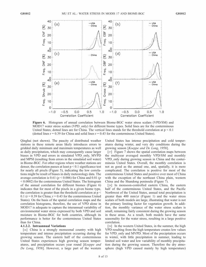
Qinghai (not shown). The paucity of distributed weatherstations in these remote areas likely introduces errors togridded daily minimum and maximum temperatures as wellas daily precipitation, which may consequently cause largerbiases in VPD and errors in simulated VPD_only, MVPDand MPSI (resulting from errors in the simulated soil water)in Biome-BGC. For other regions where weather stations aredenser, the correlation passes at least p < 0.1 significance testfor nearly all pixels (Figure 5), indicating the low correla-tions might be result of biases in daily meteorology data. Theaverage correlation is 0.61 (p < 0.006) for China and 0.81 (p< 0.0002) for the conterminous United States. The histogramof the annual correlation for different biomes (Figure 6)indicates that for most of the pixels in a given biome type,the correlation is greater than the threshold correlation at p <0.1 (r = 0.39 for China; r = 0.43 for the conterminous UnitedStates). On the basis of the spatial correlation maps and thecorrelation histograms, therefore, the use of VPD alone inMOD17 is adequate to capture the interannual variability ofenvironmental water stress expressed by both VPD and soilmoisture in Biome-BGC for both countries, although itsperformance is better for the conterminous United Statesthan for China.4.1.2.2. Intraannual Variations[26] China is a strongly monsoonal country with high

temperature and intense precipitation occurring during thegrowing season. The eastern half of the conterminousUnited States experiences high growing season temper-atures, and precipitation occurs year round [Koeppe andDe Long, 1958]. However, a large part of the western

United States has intense precipitation and cold temper-atures during winter, and very dry conditions during thegrowing season [Koeppe and De Long, 1958].[27] Figure 7 shows the spatial correlation maps between

the multiyear averaged monthly VPD/SM and monthlyVPD_only during growing season in China and the conter-minous United States. Overall, the monthly correlation isnot as good as the annual one, and, spatially, it is morecomplicated. The correlation is positive for most of theconterminous United States and positive over most of Chinawith the exception of the northeast China plain, westernChina and the Shandong peninsula (Figure 7).[28] In monsoon-controlled eastern China, the eastern

half of the conterminous United States, and the PacificNorthwest of the United States, annual total precipitation isgreater than 400 mm/yr (Figure 1) and the water stressscalars of both models are large, illustrating that water is notthe primary limiting factor for vegetation growth. In addi-tion, the monthly variance of the water stress scalars issmall, remaining fairly consistent during the growing seasonin these areas. As a result, both models have the sameseasonality for the water stress, resulting in a large positivecorrelation.[29] In the western United States, in the summer, the high

VPD resulting from the high temperature creates low valuesfor VPD_only and MVPD. Most of the precipitation occursin winter, with little precipitation in summer, leading tolimited soil water and low variability of monthly precipita-tion during the growing season. Therefore the dry atmo-sphere (high VPD caused mainly by high temperature)

Figure 6. Histogram of annual correlation between Biome-BGC water stress scalars (VPD/SM) andMOD17 water stress scalars (VPD_only) for different biome types. Solid lines are for the conterminousUnited States; dotted lines are for China. The vertical lines stands for the threshold correlation at p < 0.1(dotted lines r = 0.39 for China and solid lines r = 0.43 for the conterminous United States).

G01012 MU ET AL.: WATER STRESS IN MODIS 17 AND BIOME-BGC

8 of 13

G01012

generally coincides with dry soil conditions (low precipita-tion), and VPD alone can mimic the entire temporal waterstress for these regions, resulting in positive correlation(Figure 7).[30] In negatively correlated monsoon-controlled areas of

China, the climate is dry (Figure 1), and water limitation isstrong (Figure 3). Approximately 70% of the annual pre-cipitation is received in summer when VPD and temperatureare high [Northwest Normal University, 1984]. The mis-match between the atmospheric and soil dry/wet periods isresponsible for these negative correlation values betweentwo models, suggesting that VPD_only cannot capture theseasonality of the water stress expressed by the atmosphericVPD and the soil water in some of the strongly monsoon-controlled dry areas. The reason for the negative correlationregion in southern China (less than 3% of the country) isthat water stress is not the primary limitation to the plantgrowth. Both VPD/SM and VPD_only are very high andfairly consistent with very low monthly variability.[31] These results further illustrate that atmospheric

VPD_only captures water stress seasonality in regions withrelatively little water stress, for example, wet climate orwater-stressed regions with dry summer, but it fails torepresent the seasonality of water stress in water limitedareas with a strong summer monsoon cycle, where soilwater effects on vegetation growth should be included. Thehistograms of seasonal correlation (Figure 8) indicate that,for most pixels of each biome type, the correlation ispositive, but there are a number of negatively correlatedpixels in China. In addition, VPD_only can capture theseasonality of Biome-BGC water stress better in the coniferforests than in the broadleaf forests and other vegetationareas, because DBF are more sensitive to soil water stressthan DNF [Kljun et al., 2004].

4.2. GPP

[32] It is fairly easy for most ecosystem models to capturethe general seasonality of primary production simply

because temperature and solar radiation are used to mimicphenology [White et al., 1997; Leuning et al., 2005].Comparison of interannual variations in primary productionsimulated by different ecosystem models, however, can becomplex, because different models have different formula-tions representing ecosystem processes and environmentalstresses. More details can be found in section 2.1, 2.2 andthe work of Dargaville et al. [2002].[33] Figure 9 compares the spatial correlation maps of

multiyear averaged monthly (Figures 9a and 9b) and annual(Figures 9c and 9d) Biome-BGC simulated GPP withMOD17 estimated GPP. The GPP from the two modelsagrees better on a monthly basis than at the annual timestep. The monthly correlation is positive in most parts ofChina and the conterminous United States. The annualcorrelation (Figures 9c and 9d) is usually smaller than themonthly correlation and negative values occur in moreplaces than with the seasonal correlation in both countries(Figures 9a and 9b). Unlike water stress, GPP interannualvariability is more difficult to capture than the seasonality,because there are more factors involved in the calculation ofGPP. As discussed in section 2, the Biome-BGC andMOD17 algorithms have completely different formulationsfor calculating GPP. Biome-BGC calculates the potentialsoil moisture and GPP, and the interannual GPP variabilityis mainly driven by the variations in climate. The MOD17algorithm uses climate data and satellite-derived FPAR toestimate GPP, and satellite data can provide some informa-tion on the actual vegetation conditions, despite someuncertainties, such as navigational drift, cross calibrationof the instrument series and monthly maximum valuecompositing of FPAR. More research is needed to determinethe reasons why GPP differs between the two models.

5. Conclusion and Discussion

[34] Water stress is one of the primary limiting factorscontrolling photosynthesis by terrestrial ecosystems, and its

Figure 7. Spatial correlation between monthly Biome-BGC water stress scalars (VPD/SM) andMOD17 water stress scalars (VPD_only) during growing season in (a) China and (b) the conterminousUnited States. Vegetated regions are shown in color, and the regions in white are either nonvegetatedareas, or the areas where the standard deviation of monthly water stress scalars is less than 10�5.

G01012 MU ET AL.: WATER STRESS IN MODIS 17 AND BIOME-BGC

9 of 13

G01012

Figure 9. Monthly correlation (a) in China and (b) in the conterminous United States and annualcorrelation (c) in China and (d) in the conterminous United States between Biome-BGC GPPand MOD17 GPP during growing season. Vegetated regions are shown in color, and the regions inwhite are either nonvegetated areas, or the areas where the standard deviation of monthly GPP is less than10�5 g/m2/month or the standard deviation of annual GPP is less than 10�5 g/m2/yr.

Figure 8. Histogram of monthly correlation between Biome-BGC water stress scalars (VPD/SM) andMOD17 water stress scalars (VPD_only) for different biome types. Solid lines are for the conterminousUnited States; dotted lines are for China.

G01012 MU ET AL.: WATER STRESS IN MODIS 17 AND BIOME-BGC

10 of 13

G01012

accurate representation by ecosystem models is imperative.Ecosystem process models, such as Biome-BGC, generallycalculate the water stress as a combination of both atmo-spheric VPD and soil water limitations. Because of datalimitations, however, the global MODIS GPP/NPP algo-rithm, on the other hand, uses atmospheric VPD alone toexpress water stress. We have compared the two approachesby comparing the water stress from the MODIS algorithmwith similar results from Biome-BGC.[35] For most of the wetter areas of China and the

conterminous United States, water is not strongly limiting,and the VPD variable of the MODIS GPP algorithm reflectsthe full water stress from the air and soil as determined byBiome-BGC. Using only VPD underestimates the waterstress in dry regions where water is severely limiting, suchas western China, the northeast China plain, the Shandongpeninsula, and the central and western United States. As aresult, the MOD17 algorithm overestimates GPP in theseareas, suggesting that soil water stress may need to beconsidered to improve the GPP results. Although VPDalone fails to capture the seasonality of water stress in someareas, it reflects interannual variability in most areas,important for global carbon cycle studies and indicatingthat the current MOD17 calculations may be adequate forglobal studies.[36] The MOD17 water stress (VPD_only) captures the

interannual variability of water stress in dry regions inboth China and the conterminous United States. It reflectsthe seasonality of the water stress in the conterminousUnited States but fails in the monsoonal dry areas ofwestern China, the northeast China plain, and the Shandongpeninsula, along with some small areas of southern China,which are wetter and have strong monsoonal control. Ingeneral, VPD_only expresses the intraannual and interannualvariability of water stress in the conterminous United Statesmuch better than that in China. As a result, GPP seasonalityis captured better than interannual variability, and this sea-sonality is captured better in the conterminous United Statesthan in China. The differences between the two countriesare driven by climatic differences, such as the strongmonsoonal control of China, a climate that has not yet beentested in Biome-BGC. This leads to uncertainty in theestimates of soil and leaf water potential and, thus, theGPP from Biome-BGC, potentially affecting the results ofthis paper.[37] While the MOD17 VPD_only variable, especially

when combined with FPAR, captures water stress for mostareas of the two countries, it may be necessary to includesoil water stress in extremely dry areas. This has beendifficult in the past because of precipitation data set limi-tations, but current research with microwave remote sensingshows promise for providing accurate estimates of globalsoil moisture [Jackson, 1993; Njoku and Li, 1999], whichcan then be used as an input to the MOD17 algorithm,thereby improving GPP estimates. In addition, satelliteestimates of ET and PET [Cleugh et al., 2007; Q. Mu etal., Development of a global evapotranspiration algorithmbased on MODIS and global meteorology data, submitted toRemote Sensing of Environment, 2007] may also providemethodology to better express water stress without usingprecipitation or soil moisture.

[38] Acknowledgment. This study is funded by NASA Earth ScienceEnterprise MODIS contract (NNG04HZ19C) and Interdisciplinary ScienceProgram (NNG04GM39C).

ReferencesArora, V. (2002), Modeling vegetation as a dynamic component in soil-vegetation-atmosphere transfer schemes and hydrological models, Rev.Geophys., 40(2), 1006, doi:10.1029/2001RG000103.

Asrar, G., M. Fuchs, E. T. Kanemasu, and J. L. Hatfield (1984), Estimatingabsorbed photosynthetic radiation and leaf area index from spectralreflectance in wheat, Agron. J., 76, 300–306.

Bouchet, R. J. (1963), Evapotranspiration reele et potentielle, significationclimatique, in Proceedings of the Berkeley, California, Symposium, Publ.62, pp. 134–142, Int. Assoc. of Sci. Hydrol., Gentbrugge, Belgium.

Cao, M. K., S. D. Prince, K. Li, B. Tao, J. Small, and X. Shao (2003),Response of terrestrial carbon uptake to climate interannual variability inChina, Global Change Biol., 9, 536–546.

Chabot, B. F., and H. A. Mooney (1985), Physiological Ecology of NorthAmerican Plant Communities, CRC Press, Boca Raton, Fla.

Churkina, G., et al. (1999), Comparing global models of terrestrial netprimary productivity (NPP): The importance of water availability, GlobalChange Biol., 5, Suppl. 1, 46–55.

Cleugh, H. A., R. Leuning, Q. Mu, and S. W. Running (2007), Regionalevapotranspiration estimates from flux tower and MODIS satellite data,Remote Sens. Environ., in press.

Cosby, B. J., and G. M. Hornberger (1984), Identification of photosynthesis-light models for aquatic systems, I. Theory and simulations, Ecol. Modell.,23, 1–24.

Cramer, W., et al. (1999), Comparing global models of terrestrial net pri-mary productivity (NPP): Overview and key results, Global ChangeBiol., 5, Suppl. 1, 1–15.

Cromer, R. N., D. M. Cameron, S. J. Rance, P. A. Ryan, and M. Brown(1993), Response to nutrients in Eucalyptus grandis. 1. Biomass accu-mulation, For. Ecol. Manage., 62, 211–230.

Dang, Q. L., H. A. Margolis, M. R. Coyea, M. Sy, and G. J. Collatz (1997),Regulation of branch-level gas exchange of boreal trees: Roles of shootwater potential and vapour pressure difference, Tree Physiol., 17, 521–535.

Dargaville, R. J., et al. (2002), Evaluation of terrestrial carbon cycle modelswith atmospheric CO2 measurements: Results from transient simulationsconsidering increasing CO2, climate, and land-use effects, Global Bio-geochem. Cycles, 16(4), 1092, doi:10.1029/2001GB001426.

De Fries, R. S., M. Hansen, J. R. G. Townshend, and R. Sohlberg (1998),Global land cover classifications at 8 km spatial resolution: The use oftraining data derived from Landsat imagery in decision tree classifiers,Int. J. Remote Sens., 19(16), 3141–3168.

De Pury, D. G. G., and G. D. Farquhar (1997), Simple scaling of photo-synthesis from leaves to canopies without the errors of big-leaf models,Plant Cell Environ., 20, 537–557.

Douglas, O. F., and S. D. Prince (1996), Rainfall and foliar dynamics intropical southern Africa: Potential impacts of global climate change onsavanna vegetation, Clim. Change, 33(1), 69–96.

Field, C. B., J. T. Randerson, and C. M. Malmstrom (1995), Global netprimary production: Combining ecology and remote sensing, RemoteSens. Environ., 51, 74–88.

Friedl, M. A., et al. (2002), Global land cover mapping from MODIS:Algorithms and early results, Remote Sens. Environ., 83, 287–302.

Goward, S. N., C. J. Tucker, and D. G. Dye (1985), North Americanvegetation patterns observed with the NOAA-7 Advanced Very HighResolution Radiometer, Vegetatio, 64, 3–14.

Granger, R. J., and D. M. Gray (1989), Evaporation from natural nonsatu-rated surfaces, J. Hydrol., 111, 21–29.

Heinsch, F. A., et al. (2006), Evaluation of remote sensing based terrestrialproductivity from MODIS using tower eddy flux network observations,IEEE Trans. Geosci. Remote Sens., 44, 1908 – 1925, doi:10.1109/TGRS.2005.85396.

Hou, X. Y. (Ed.) (1980), Chinese Vegetation, Science, Beijing.Jackson, T. J. (1993), Measuring surface soil moisture using passive micro-wave remote sensing, Hydrol. Processes, 7, 139–152.

Janowiak, J. E., R. E. Livezey, A. G. C. Kondragunta, and G. J. Huffman(1998), Comparison of reanalysis precipitation with rain gauge andsatellite observations, in Proceedings of the First World Climate ResearchProgram International Conference on Reanalyses, WCRP-104, pp. 207–210, World Clim. Res. Program, World Meteorol. Org., Geneva.

Kawamitsu, Y., S. Yoda, and W. Agata (1993), Humidity pretreatmentaffects the responses of stomata and CO2 assimilation to vapor pressuredifference in C3 and C4 plants, Plant Cell Physiol., 34(1), 113–119.

Kimball, J., S. W. Running, and R. Nemani (1997a), An improved methodfor estimating surface humidity from daily minimum temperature, Agric.For. Meteorol., 85, 87–98.

G01012 MU ET AL.: WATER STRESS IN MODIS 17 AND BIOME-BGC

11 of 13

G01012

Kimball, J. S., P. E. Thornton, M. A. White, and S. W. Running (1997b),Simulating forest productivity and surface-atmosphere carbon exchangein the BOREAS study region, Tree Physiol., 17, 589–599.

Kimball, J. S., M. A. White, and S. W. Running (1997c), BIOME-BGCsimulations of stand hydrologic processes for BOREAS, J. Geophys.Res., 102(D24), 29,043–29,052.

Kljun, N., T. A. Black, T. J. Griffis, A. G. Barr, D. Gaumont-Guay,K. Morgenstern, J. H. McCaughey, and Z. Nesic (2004), Net carbonexchange of three boreal forests during a drought, paper presented at26th Conference on Agricultural and Forest Meteorology, Am. Meteorol.Soc., Boston, Mass.

Koeppe, C. E., and G. C. De Long (1958), Weather and Climate, McGraw-Hill, New York.

Korner, C. (1995), Leaf diffusive conductances in the major vegetationtypes of the globe, in Ecophysiology of Photosynthesis, edited by E.-D.Schulze and M. M. Caldwell, pp. 463–490, Springer, New York.

Kumar, M., and J. L. Monteith (1982), Remote sensing of crop growth,in Plants and Daylight Spectrum, edited by H. Smith, pp. 133–144,Elsevier, New York.

Landsberg, J. J. (1986), Physiological Ecology of Forest Production,Elsevier, New York.

Landsberg, J. (1999), The Ways Trees Use Water, Water Salinity IssuesAgrofor., vol. 5, Rural Ind. Res. Dev. Corp., Kingston, ACT, Australia.(Available at http://www.rirdc.gov.au/reports/AFT/99-37.pdf)

Lange, O. L., W. Beyschlag, and J. D. Tenhunen (1987), Control of leafcarbon assimilation—Input of chemical energy into ecosystem, in Poten-tials and Limitations of Ecosystem Analysis, edited by E.-D. Schulze andH. Zwolfer, pp. 149–163, Springer, New York.

Leuning, R., F. M. Kelliher, D. G. G. Pury, and E.-D. Schulze (1995), Leafnitrogen, photosynthesis, conductance and transpiration: Scaling fromleaves to canopies, Plant Cell Environ., 18, 1183–1200.

Leuning, R., H. A. Cleugh, S. J. Zegelin, and D. Hughes (2005), Carbonand water fluxes over a temperate Eucalyptus forest and a tropical wet/dry savanna in Australia: Measurements and comparison with MODISremote sensing estimates, Agric. For. Meteorol., 129, 151–173.

Marsden, B. J., V. J. Lieffers, and J. J. Zwiazek (1996), The effect ofhumidity on photosynthesis and water relations of white spruce seedlingsduring the early establishment phase, Can. J. For. Res., 26, 1015–1021.

Misson, L., J. A. Panek, and A. H. Goldstein (2004), A comparison of threeapproaches to modeling leaf gas exchange in annually drought-stressedponderosa pine forests, Tree Physiol., 24, 529–541.

Monteith, J. L. (1972), Solar radiation and productivity in tropical ecosys-tems, J. Appl. Ecol., 9, 747–766.

Monteith, J. L. (1977), Climate and efficiency of crop production in Britain,Philos. Trans. R. Soc., Ser. B, 281, 277–294.

Morton, F. I. (1983), Operational estimates of areal evapotranspiration andtheir significance to the science and practice of hydrology, J. Hydrol., 66,1–76.

Myers, B. J., S. Theiveyanathan, N. D. O’Brien, and W. J. Bond (1996),Growth and water use of Eucalyptus grandis and Pinus radiata planta-tions irrigated with effluent, Tree Physiol., 16, 211–219.

Myneni, R. B., R. R. Nemani, and S. W. Running (1997), Estimation ofglobal leaf area index and absorbed par using radiative transfer models,IEEE Trans. Geosci. Remote Sens., 35, 1380–1393.

Nemani, R. R., S. W. Running, R. A. Pielke, and T. N. Chase (1996),Global vegetation cover changes from coarse resolution satellite data,J. Geophys. Res., 101(D3), 7157–7162.

Nemani, R., M. White, P. Thornton, K. Nishida, S. Reddy, J. Jenkins, andS. Running (2002), Recent trends in hydrologic balance have enhancedthe terrestrial carbon sink in the United States, Geophys. Res. Lett.,29(10), 1468, doi:10.1029/2002GL014867.

Nemani, R. R., C. Keeling, H. Hashimoto, W. M. Jolly, S. Piper, C. Tucker,R. Myneni, and S. W. Running (2003), Climate-driven increases in globalterrestrial net primary production from 1982 to 1999, Science, 300,1560–1563.

New, M., M. Hulme, and P. Jones (2000), Representing twentieth-centuryspace-time climate variability. Part II: Development of 1901–1996monthly grids of terrestrial surface climate, J. Clim., 13(13), 2217–2238.

Nicholson, S. E., C. J. Tucker, and M. B. Ba (1998), Desertification,drought, and surface vegetation: An example from the West AfricanSahel, Bull. Am. Meteorol. Soc., 79(5), 815–829.

Njoku, E., and L. Li (1999), Retrieval of land surface parameters usingpassive microwave measurements at 6–18 GHz, IEEE Trans. Geosci.Remote Sens., 37, 79–93.

Northwest Normal University (Eds.) (1984), Chinese Atlas of PhysicalGeography, 200 pp., China Cartogr. Publ. House, Beijing.

Oren, R., J. S. Sperry, G. G. Katul, D. E. Pataki, B. E. Ewers, N. Phillips,and K. V. R. Schafer (1999), Survey and synthesis of intra- and inter-specific variation in stomatal sensitivity to vapour pressure deficit, PlantCell Environ., 22, 1515–1526.

Paruelo, J. M., and W. K. Lauenroth (1995), Regional pattern of normalizeddifference vegetation index in North American shrublands and grass-lands, Ecology, 76(6), 1888–1898.

Potter, C. S., J. T. Randerson, C. B. Field, P. A. Matson, P. M. Vitousek,H. A. Mooney, and S. A. Klooster (1993), Terrestrial ecosystem produc-tion: A process model based on global satellite and surface data, GlobalBiogeochem. Cycles, 7(4), 811–842.

Prentice, I. C., et al. (2001), The carbon cycle and atmospheric carbondioxide, in Climate Change 2001: The Scientific Basis—Contributionof Working Group I to the Third Assessment Report of the Intergovern-mental Panel on Climate Change, edited by J. T. Houghton et al., pp.182–237, Cambridge Univ. Press, New York.

Prince, S. D., and S. N. Goward (1995), Global primary production: Aremote sensing approach, J. Biogeogr., 22, 815–835.

Rastetter, E. B., A. W. King, B. J. Cosby, G. M. Hornberger, R. V. O’Neill,and J. E. Hobbie (1992), Aggregating fine-scale ecological knowledge tomodel coarser-scale attributes of ecosystems, Ecol. Appl., 2(1), 55–70.

Ruimy, A., B. Saugier, and G. Dedieu (1994), Methodology for the estima-tion of terrestrial net primary production from remotely sensed data,J. Geophys. Res., 99(D3), 5263–5284.

Running, S. W., and E. R. Hunt (1993), Generalization of a forest ecosys-tem process model for other biomes, Biome-BGC, and an applicationfor global-scale models, in Scaling Physiological Processes: Leaf toGlobe, edited by J. R. Ehleringer and C. B. Field, pp. 141–158,Elsevier, New York.

Running, S. W., and J. S. Kimball (2005), Satellite-based analysis ofecological controls for land-surface evaporation resistance, in Encyclope-dia of Hydrological Sciences, vol. 3, chap. 104, pp. 1587–1600, editedby M. Anderson, John Wiley, Hoboken, N. J.

Running, S. W., and R. R. Nemani (1988), Relating seasonal patterns of theAVHRRVegetation Index to simulate photosynthesis and transpiration offorests in different climates, Remote Sens. Environ., 24, 347–367.

Running, S. W., P. E. Thornton, R. R. Nemani, and J. M. Glassy (2000),Global terrestrial gross and net primary productivity from the EarthObserving System, in Methods in Ecosystem Science, edited by O. Salaet al., pp. 44–57, Springer, New York.

Running, S. W., R. R. Nemani, F. A. Heinsch, M. Zhao, M. Reeves, andH. Hashimoto (2004), A continuous satellite-derived measure of globalterrestrial primary productivity: Future science and applications,BioScience, 56(6), 547–560.

Schultz, P. A., and M. S. Halpert (1995), Global analysis of the relation-ships among a vegetation index, precipitation, and land surface tempera-ture, Int. J. Remote Sens., 16, 2755–2777.

Sellers, P. J. (1987), Canopy reflectance, photosynthesis and transpiration.II. The role of biophysics in the linearity of their interdependence, RemoteSens. Environ., 21, 143–183.

Sellers, P. J., J. A. Berry, G. J. Collatz, C. B. Field, and F. G. Hall (1992),Canopy reflectance, photosynthesis, and transpiration. III. A reanalysisusing improved leaf models and a new canopy integration scheme,Remote Sens. Environ., 42, 187–216.

Sinclair, T. R., C. E. Murphy, and K. R. Knoerr (1976), Development andevaluation of simplified models for simulating canopy photosynthesisand transpiration, J. Appl. Ecol., 13, 813–829.

Tao, B., et al. (2003), The temporal and spatial patterns of terrestrial netprimary productivity in China, J. Geogr. Sci., 13(2), 163–171.

Thornton, P. E., and S. W. Running (1999), An improved algorithm forestimating incident daily solar radiation from measurements of tempera-ture, humidity, and precipitation, Agric. For. Meteorol., 93, 211–228.

Thornton, P. E., S. W. Running, and M. A. White (1997), Generatingsurfaces of daily meteorology variables over large regions of complexterrain, J. Hydrol., 190, 214–251.

Thornton, P. E., et al. (2002), Modeling and measuring the effects of dis-turbance history and climate on carbon and water budgets in evergreenneedle leaf forests, Agric. For. Meteorol., 113, 185–222.

Turner, D. P., W. D. Ritts, W. B. Cohen, S. T. Gower, M. Zhao, S. W.Running, S. C. Wofsy, S. Urbanski, A. L. Dunn, and J. W. Munger(2003), Scaling gross primary production (GPP) over boreal and decid-uous forest landscapes in support of MODIS GPP product validation,Remote Sens. Environ., 88, 256–270.

Turner, D. P., et al. (2005), Site-level evaluation of satellite-based globalterrestrial GPP and NPP monitoring, Global Change Biol., 11, 666–684.

Turner, D. P., W. Ritts, M. Zhao, S. Kurc, A. Dunn, S. Wofsy, E. Small, andS. W. Running (2006), Assessing interannual variation in MODIS-basedestimates of gross primary production, IEEE Trans. Geosci. RemoteSens., 44, 1899–1907.

Vorosmarty, C. J., C. A. Federer, and A. L. Schloss (1998), Potential eva-poration function compared on US watersheds: Possible implication forglobal-scale water balance and terrestrial ecosystem, J. Hydrol., 207,147–169.

G01012 MU ET AL.: WATER STRESS IN MODIS 17 AND BIOME-BGC

12 of 13

G01012

Wang, S., H. Q. Tian, J. Liu, and S. Pan (2003), Pattern and change in soilorganic carbon storage in China: 1960s–1980s, Tellus, Ser. B, 55, 416–427.

Wang, Y. P., and P. J. Jarvis (1993), Influence of shoot structure on photo-synthesis of Sitka spruce (Picea sitchensis), Funct. Ecol., 7, 433–451.

Waring, R., and S. W. Running (1998), Forest Ecosystems: Analysis atMultiple Scales, Elsevier, New York.

White, M. A., P. E. Thornton, and S. W. Running (1997), A continentalphenology model for monitoring vegetation responses to interannual cli-matic variability, Global Biogeochem. Cycles, 11(2), 217–234.

White, M. A., P. E. Thornton, S. W. Running, and R. R. Nemani (2000),Parameterization and sensitivity analysis of the BIOME–BGC terrestrialecosystem model: Net primary production controls, Earth Interact., 4(3),doi:10.1175/1087-3562(2000)004<0003:PASAOT>2.0.CO;2.

Wong, S. C., I. R. Cowan, and G. D. Farquhar (1985a), Leaf conductance inrelation to rate of CO2 assimilation. I. Influence of nitrogen nutrition,phosphorus nutrition, photon flux density, and ambient partial pressure ofCO2 during ontogeny, Plant Physiol., 78, 821–825.

Wong, S. C., I. R. Cowan, and G. D. Farquhar (1985b), Leaf conductance inrelation to rate of CO2 assimilation. II. Effects of short-term exposure todifferent photon flux densities, Plant Physiol., 78, 826–829.

Wong, S. C., I. R. Cowan, and G. D. Farquhar (1985c), Leaf conductance inrelation to rate of CO2 assimilation. III. Influence of water stress andphotoinhibition, Plant Physiol., 78, 830–834.

Zhang, C., H. Tian, J. Liu, S. Wang, M. Liu, S. Pan, and X. Shi (2005),Pools and distributions of soil phosphorus in China, Global Biogeochem.Cycles, 19, GB1020, doi:10.1029/2004GB002296.

Zhao, M., C. Fu, X. Yan, and G. Wen (2001), Study on the relationshipbetween different ecosystems and climate in China using NOAA/AVHRRdata, Acta Geogr. Sin., 56(3), 287–296.

Zhao, M., F. A. Heinsch, R. R. Nemani, and S. W. Running (2005),Improvements of the MODIS terrestrial gross and net primary productionglobal data set, Remote Sens. Environ., 95, 164–176.

Zhao, M., S. W. Running, and R. R. Nemani (2006), Sensitivity of Mod-erate Resolution Imaging Spectroradiometer (MODIS) terrestrial primaryproduction to the accuracy of meteorological reanalyses, J. Geophys.Res., 111, G01002, doi:10.1029/2004JG000004.

�����������������������F. A. Heinsch, Q.Mu, S.W. Running, andM. Zhao, Numerical Terradynamic

Simulation Group, Department of Ecosystem and Conservation Sciences,University of Montana, Missoula, MT 59812, USA. (qiaozhen@ntsg.umt.edu)Q.-M. Liu and H. Tian, School of Forestry and Wildlife Sciences, Auburn

University, Auburn, AL 36849, USA.

G01012 MU ET AL.: WATER STRESS IN MODIS 17 AND BIOME-BGC

13 of 13

G01012