arX

iv:c

s/06

0611

5v1

[cs

.AI]

28

Jun

2006

Evaluating Variable Length Markov Chain

Models for Analysis of User Web Navigation

Sessions

Jose Borges ∗

School of Engineering,

University of Porto

R. Dr. Roberto Frias, 4200 - Porto, Portugal

jlborges@fe.up.pt

Mark Levene

School of Computer Science and Information Systems,

Birkbeck, University of London

Malet Street, London WC1E 7HX, U.K.

mark@dcs.bbk.ac.uk

February 1, 2008

∗Supported by the POSC/EIA/58367/2004/Site-o-Matic Project (Fundacao Ciencia eTecnologia) co-financed by FEDER.

1

Abstract

Markov models have been widely used to represent and analyse

user web navigation data. In previous work we have proposed a

method to dynamically extend the order of a Markov chain model and

a complimentary method for assessing the predictive power of such a

variable length Markov chain. Herein, we review these two methods

and propose a novel method for measuring the ability of a variable

length Markov model to summarise user web navigation sessions up

to a given length. While the summarisation ability of a model is im-

portant to enable the identification of user navigation patterns, the

ability to make predictions is important in order to foresee the next

link choice of a user after following a given trail so as, for example,

to personalise a web site. We present an extensive experimental eval-

uation providing strong evidence that prediction accuracy increases

linearly with summarisation ability.

1 Introduction

Web usage mining has been defined as the research field focused on developing

techniques to model and study users’ web navigation data [Mob04]. Data

characterising user web navigation sessions can be collected from server log

files or from a web browser plug-in aimed at recording the user navigation

options. From the collected data it is possible to reconstruct users’ web

navigation sessions [SMBN03], where a session, also referred to as a trail,

consists of a sequence of web pages viewed by a user within a given time

window.

2

Several models have been proposed for modelling user web data. Schechter

et al. [SKS98] utilised a tree-based data structure that represents the col-

lection of paths inferred from the log data to predict the next page access.

Dongshan and Junyi [DJ02] proposed a hybrid-order tree-like Markov model,

which provides good scalability and high coverage of the state-space, also to

predict the next page access. Chen and Zhang [CZ03] utilised a PPM (Pre-

diction by Partial Match) forest that restricts the roots to popular nodes;

assuming that most user sessions start with popular pages, they reduce the

model complexity by eliminating branches having a non-popular page as their

root. [DK04] proposed a technique that builds kth−order Markov models and

combines them to include the highest order model covering each state; they

also develop techniques to eliminate states and reduce the model complexity.

In [EVK05] the authors propose a method that incorporates link analysis,

such as the pagerank measure, into a Markov model in order to provide web

path recommendations.

In [BL00] we have proposed a first-order Markov model for a collection of

user navigation sessions, and more recently we have extended the method to

represent higher-order conditional probabilities by making use of a cloning

operation [BL05a, BL05b]. In addition, we have proposed a method to evalu-

ate the predictive power of a model that takes into account a variable length

history when estimating the probability of the next link choice of a user,

given his/her navigation trail [BL06]. (We review these models in subsec-

tions 2.1 and 2.2.) Herein, we propose a new method to measure the sum-

marisation ability of a model, by which we mean the ability of a variable

length Markov model to summarise user web navigation sessions up to a

3

given length. Briefly, from a collection of user web navigation trails a vari-

able length Markov model, up to order n, is built, and an algorithm is devised

to induce the user trails having a high probability of being traversed. The

set of trails is then ranked, from the most to least probable, and the re-

sulting ranking is compared with the ranking induced from input trails of

length n, i.e. from the n-gram frequency count of the input trails. Thus, if a

model accurately represents the collection of input navigation trails of length

n, the two rankings should be identical. Note that while it is clear that a

n-order Markov model accurately represents trails shorter or equal to n, it

is important to understand how well such a model represents trails longer

than n. To make the comparison between the rankings we use the Spear-

man footrule [FKS03] and percentage overlap metrics. We present the results

of an extensive experimental evaluation conducted on three real world data

sets, which provides strong evidence that the measure of predictive power

increases linearly with the measure for summarisation ability.

Understanding the behaviour of web site visitors navigating through the

site is an important step in the process of improving the quality of service

of the site. In our opinion Markov models are well suited for modelling user

web navigation data because they are compact, simple to understand and

motivate, expressive and based on a well established theory. Commercial

tools for log data analysis usually discard the information concerning the

order in which page views occurred in a session and the same can be said

about the techniques using association rules methods. On the other hand,

variable length Markov chain models provide the probability of the next link

chosen when viewing a web page, while taking into account the trail followed

4

to reach that page.

Our measure of the summarisation ability of the model answers a question

we have often been asked about the adequacy of Markov models in represent-

ing user web trails. The measure tells us how accurate is the Markov model

representing the users’ trails, and, thus, when having a precise Markov rep-

resentation we are justified in using methods that extract the most probable

trails from the model, see [BL04]. Such trail patterns can, for example, pro-

vide guidelines for improving the static structure of a web site. Moreover,

Markov models can also be used to predict the user’s next navigation step

within the site, as is shown in Section 2.4. Such methods can be also used

for web site personalisation by adapting the web page presentation to the

profile of the current user. Thus, the summarisation ability of the model is

important for enabling the identification of user navigation patterns, and the

prediction ability is important for foreseeing the next link choice of a user

after following a given trail.

We stress that there has been previous research on evaluating the ability

of a Markov model to predict the next link choice of a user, [DK04, BL06],

however, to the best of our knowledge, there is a lack of publications on

evaluating the ability of a Markov model to represent user sessions up to a

given history length. Moreover, as far as we know, the relationship between

summarisation ability and prediction power has not been studied before in

the context of web mining.

The rest of the paper is organised as follows. In Section 2 we introduce

the variable length Markov chain methods we make use of. More specifically,

in subsection 2.1 we introduce our method for building a first-order model

5

from a collection of user sessions, in subsection 2.2 we introduce our extension

of the method to higher-order conditional probabilities, in subsection 2.3 we

present our new method for measuring the model’s summarisation ability,

and in subsection 2.4 we introduce our method for measuring the model’s

predictive power. In Section 3 we present an experimental evaluation of

these methods, and, finally, in Section 4 we give our concluding remarks.

2 Variable Length Markov Chains Methods

A user navigation session within a web site can be represented by the sequence

of pages requested by the user. First-order Markov models have been widely

used to model a collection of user sessions. In such a model each web page in

the site corresponds to a state in a first-order Markov model, and each pair

of pages viewed in sequence corresponds to a state transition in the model.

Each transition probability is estimated by the ratio of the number of times

the transition was traversed and the number of times the first state in the

pair was visited. Usually, an artificial state is appended to every navigation

session to denote the start and finish of the session.

A first-order Markov model is a compact way of representing a collec-

tion of sessions but in most cases its accuracy is low [JPT03], which is why

extensions to higher-order Markov models are necessary to improve the ac-

curacy. In a (non-variable) higher-order Markov model a state corresponds

to a fixed sequence of pages, and transition between two states represents a

higher-order conditional probability [BL00]. For example, in a second-order

model each state corresponds to a sequence of two page views. The serious

6

drawback of fixed higher-order Markov models is their exponentially large

state space compared to lower-order models.

A variable length Markov chain (VLMC) is a model extension that al-

lows variable length history to be captured [Bej04]. In [BL05b] we proposed

a method that transforms a first-order model into a VLMC so that each

transition probability between two states takes into account the path a user

followed to reach the first state prior to choosing the outlink corresponding

to the transition to the second state. The method makes use of state cloning

(where states are duplicated to distinguish between different paths leading

to the same state) together with a clustering technique that separates paths

revealing differences in their conditional probabilities. We will now introduce

our method by means of an illustrative example; we refer readers looking for

a formal description of the method to [BL05b].

2.1 First-Order Model Construction

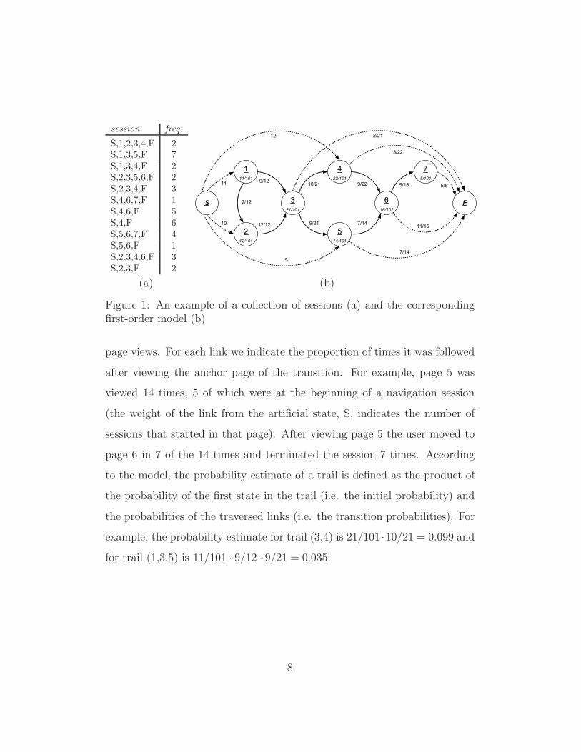
Figure 1 (a) shows an example of a collection of user navigation sessions. We

let a session start and finish at an artificial state and, for each session, we give

the number of times the corresponding sequence of pages was traversed by

a user (freq.). Figure 1 (b) presents the first-order model for these sessions.

There is a state corresponding to each web page and a link connecting every

two pages viewed in sequence. For each state that corresponds to a web page

we give the page identifier and the number of times the page was viewed

divided by the total number of page views. This ratio is an estimate of the

probability of a user choosing the corresponding page from the set of all pages

in the web site. For example, page 4 has 22 page views from a total of 101

7

session freq.

S,1,2,3,4,F 2S,1,3,5,F 7S,1,3,4,F 2S,2,3,5,6,F 2S,2,3,4,F 3S,4,6,7,F 1S,4,6,F 5S,4,F 6S,5,6,7,F 4S,5,6,F 1S,2,3,4,6,F 3S,2,3,F 2

(a)

1

11/101

2

12/101

5

14/101

3

21/101

4

22/101

S F6

16/101

7

5/101

119/12

2/12

10 12/12 9/21

10/21

2/21

9/22

13/22

12

5

7/14

7/14

5/55/16

11/16

(b)

Figure 1: An example of a collection of sessions (a) and the correspondingfirst-order model (b)

page views. For each link we indicate the proportion of times it was followed

after viewing the anchor page of the transition. For example, page 5 was

viewed 14 times, 5 of which were at the beginning of a navigation session

(the weight of the link from the artificial state, S, indicates the number of

sessions that started in that page). After viewing page 5 the user moved to

page 6 in 7 of the 14 times and terminated the session 7 times. According

to the model, the probability estimate of a trail is defined as the product of

the probability of the first state in the trail (i.e. the initial probability) and

the probabilities of the traversed links (i.e. the transition probabilities). For

example, the probability estimate for trail (3,4) is 21/101 ·10/21 = 0.099 and

for trail (1,3,5) is 11/101 · 9/12 · 9/21 = 0.035.

8

S F

7

5/101

12/12

2/9

2/12

7/10

12

57/9

2/9

1/9

8/9

5/5

9/11

8/12

2/12

5/5

3/7

4/7

6/12

6/12

11 3

9/101

3'

12/101

4

10/101

4'

12/101

5

9/101

5'

5/101

6

9/101

6'

7/101

7/9

3/10

10

1

11/101

2

12/101

2/11

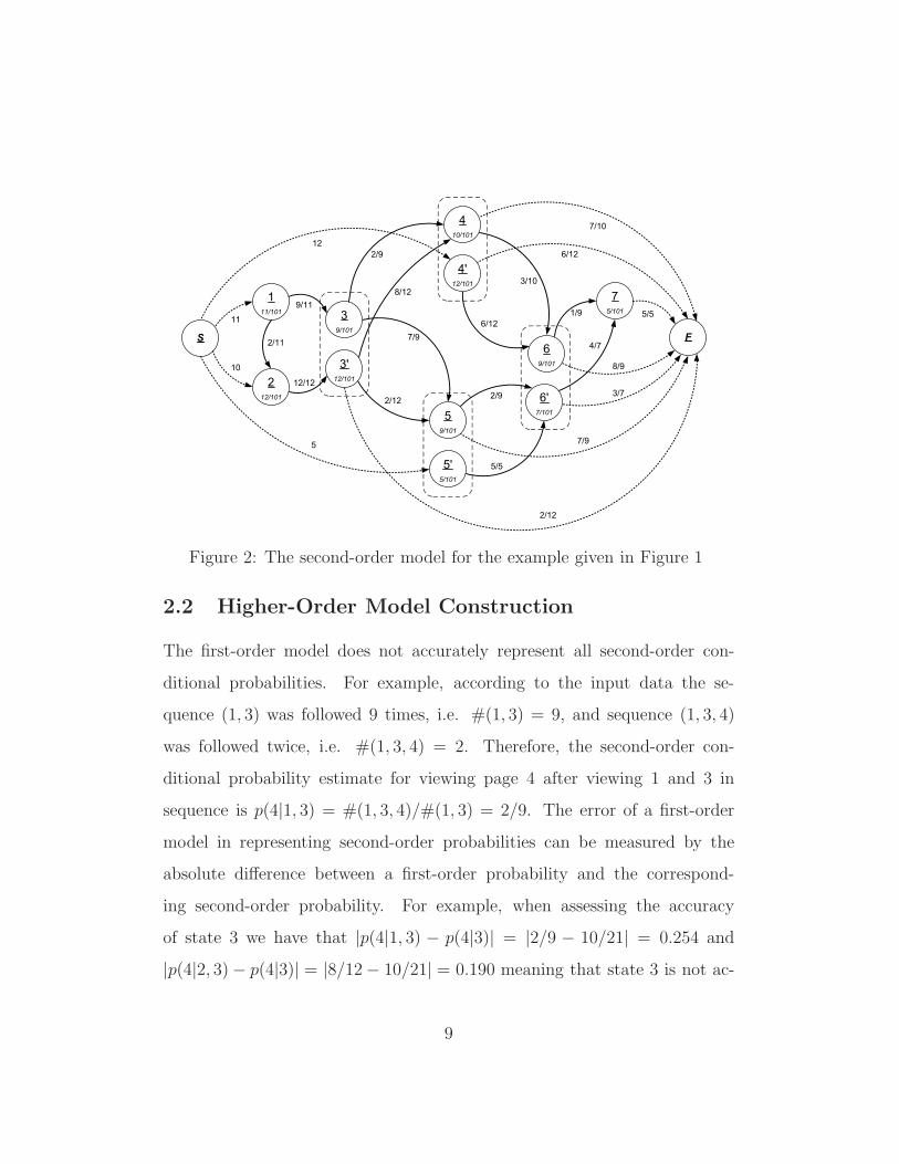
Figure 2: The second-order model for the example given in Figure 1

2.2 Higher-Order Model Construction

The first-order model does not accurately represent all second-order con-

ditional probabilities. For example, according to the input data the se-

quence (1, 3) was followed 9 times, i.e. #(1, 3) = 9, and sequence (1, 3, 4)

was followed twice, i.e. #(1, 3, 4) = 2. Therefore, the second-order con-

ditional probability estimate for viewing page 4 after viewing 1 and 3 in

sequence is p(4|1, 3) = #(1, 3, 4)/#(1, 3) = 2/9. The error of a first-order

model in representing second-order probabilities can be measured by the

absolute difference between a first-order probability and the correspond-

ing second-order probability. For example, when assessing the accuracy

of state 3 we have that |p(4|1, 3) − p(4|3)| = |2/9 − 10/21| = 0.254 and

|p(4|2, 3) − p(4|3)| = |8/12 − 10/21| = 0.190 meaning that state 3 is not ac-

9

curately representing second-order conditional probabilities. To address this

problem the accuracy of the transition probabilities can be increased by sep-

arating the in-paths to the state corresponding to the different conditional

probabilities. In this example increased accuracy can be achieved by cloning

state 3 (i.e. creating a duplicate state 3’) and redirecting the link (2,3) to

state 3’. The weights of the outlinks from states 3 and 3’ are updated ac-

cording to the number of times the sequence of three states was followed.

For example, since #(1, 3, 4) = 2 and #(1, 3, 5) = 7 in the second-order

model, the weight of the link (3,4) is 2 and the weight of (3,5) is 7. (Note

that, according to the input data, no session terminates at page 3 when the

user has navigated to it from page 1.) The same method is applied to up-

date the outlinks from the clone state 3’. Figure 2 shows the second-order

model corresponding to the collection of sessions given in our example af-

ter four states were cloned in order to accurately represent all second-order

conditional probabilities.

In the extended model given in Figure 2 all the outlinks represent the

correct second-order probabilities estimates. The probability estimate of the

trail (1,3,5) is now 11/101 · 9/11 · 7/9 = 0.069. The probability estimate for

trail (3,4) is computed as (9/101 · 2/9) + (12/101 · 8/12) = 0.099 which is

equal to the probability estimate given by the first-order model, noting that

state 3’ is a clone of 3. Therefore, the second-order model accurately models

the conditional second-order probabilities estimates while keeping the correct

first-order probability estimates.

In order to provide control over the number of additional states created by

the method we make use of a parameter, γ, that sets the highest admissible

10

difference between a first-order and the corresponding second-order proba-

bility estimate. In a first-order model, when assessing the accuracy of a state

the state is cloned if there is a second-order probability whose difference to

the corresponding first-order probability is greater than γ. Alternatively, we

interpret γ as a threshold for the average difference between the first-order

and the corresponding second-order probabilities for a given state. In the

latter, the state is cloned if the average difference between first and second-

order conditional probabilities surpasses γ. Moreover, if we set γ > 0 and

the state has three or more inlinks we make use of a clustering algorithm

to identify inlinks inducing identical conditional probabilities. When γ is

measuring the maximum probability of divergence, we will denote it by γm

and when it is measuring the average probability divergence, we will denote

it by γa.

session freq.

1,2,3 31,2,5 14,2,3 44,2,5 26,2,3 16,2,5 3

(a)

1

24

6

3

5

4/4

4/4

6/6

8/14

6/14

(b)

1

2

4

6

3

52'

4/4

6/6

4/4

7/10

3/4

1/4

3/10

(c)

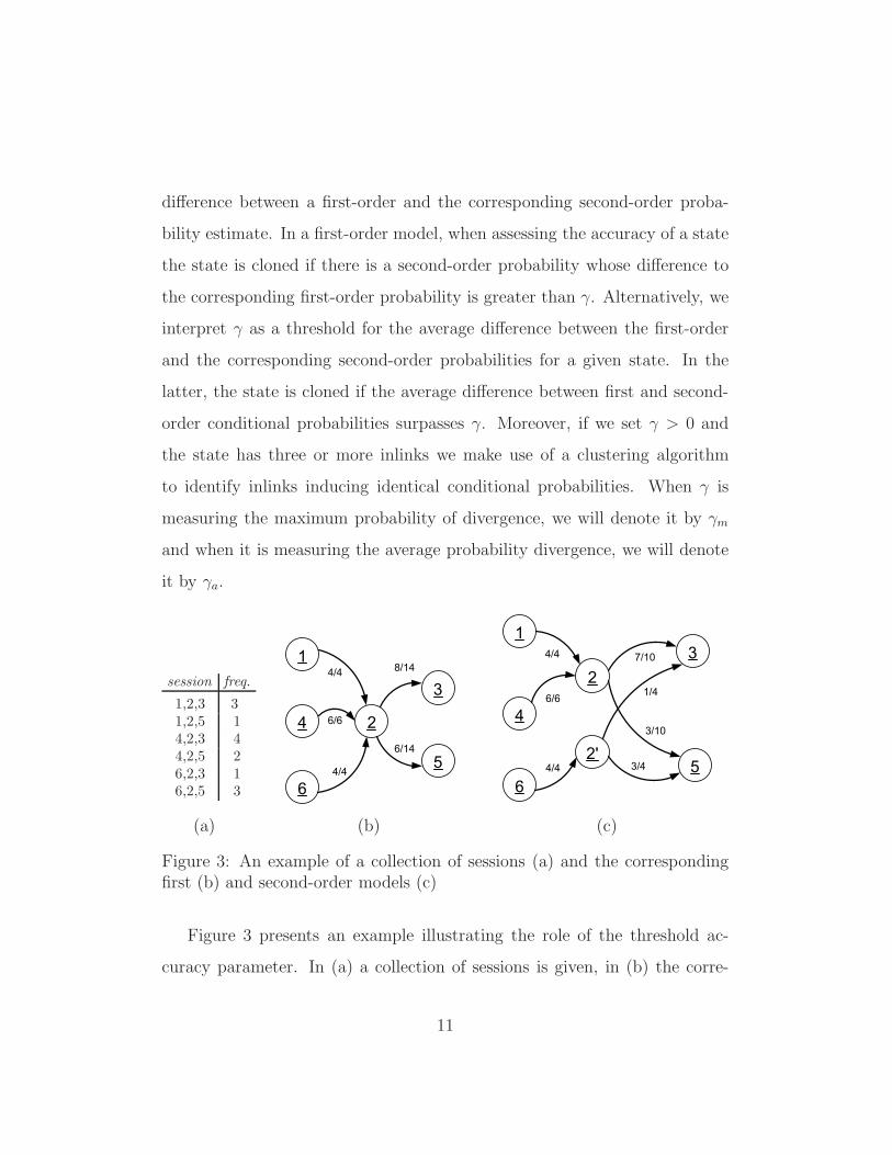
Figure 3: An example of a collection of sessions (a) and the correspondingfirst (b) and second-order models (c)

Figure 3 presents an example illustrating the role of the threshold ac-

curacy parameter. In (a) a collection of sessions is given, in (b) the corre-

11

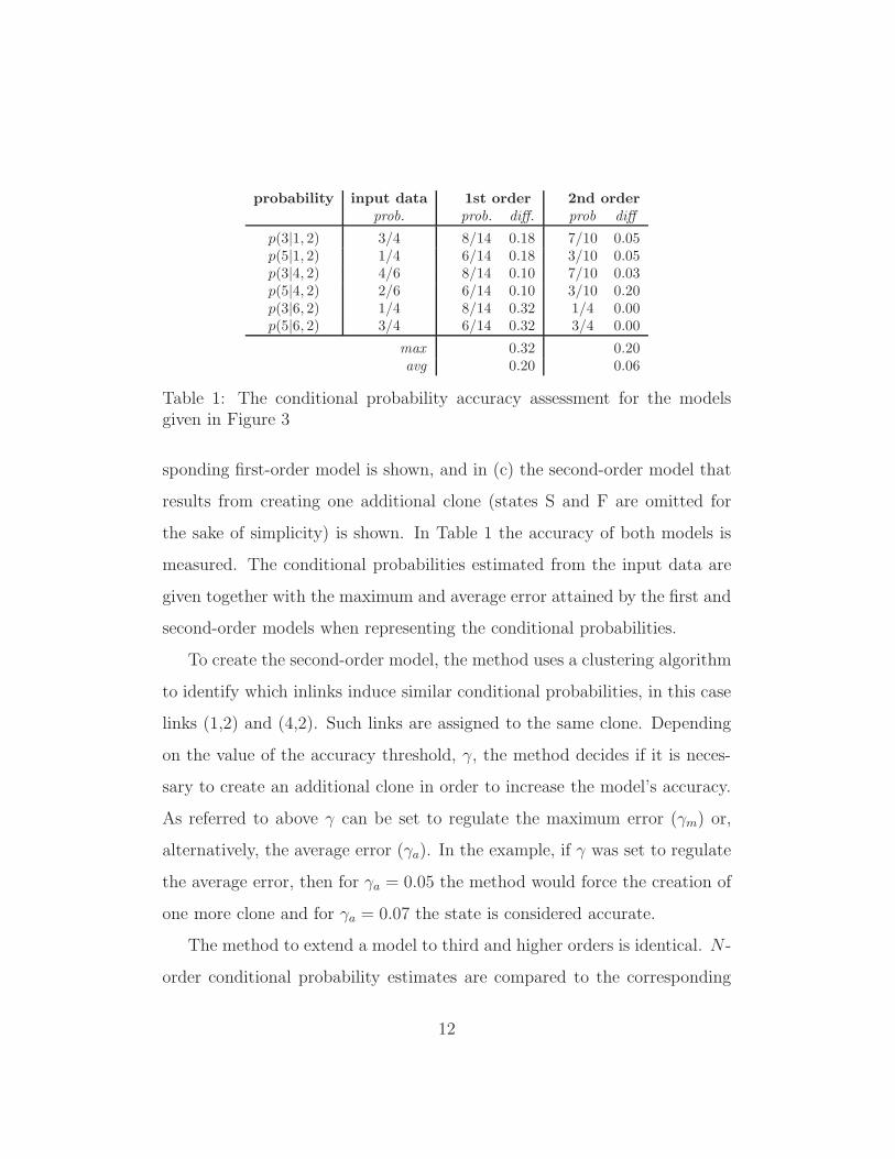
probability input data 1st order 2nd order

prob. prob. diff. prob diff

p(3|1, 2) 3/4 8/14 0.18 7/10 0.05p(5|1, 2) 1/4 6/14 0.18 3/10 0.05p(3|4, 2) 4/6 8/14 0.10 7/10 0.03p(5|4, 2) 2/6 6/14 0.10 3/10 0.20p(3|6, 2) 1/4 8/14 0.32 1/4 0.00p(5|6, 2) 3/4 6/14 0.32 3/4 0.00

max 0.32 0.20avg 0.20 0.06

Table 1: The conditional probability accuracy assessment for the modelsgiven in Figure 3

sponding first-order model is shown, and in (c) the second-order model that

results from creating one additional clone (states S and F are omitted for

the sake of simplicity) is shown. In Table 1 the accuracy of both models is

measured. The conditional probabilities estimated from the input data are

given together with the maximum and average error attained by the first and

second-order models when representing the conditional probabilities.

To create the second-order model, the method uses a clustering algorithm

to identify which inlinks induce similar conditional probabilities, in this case

links (1,2) and (4,2). Such links are assigned to the same clone. Depending

on the value of the accuracy threshold, γ, the method decides if it is neces-

sary to create an additional clone in order to increase the model’s accuracy.

As referred to above γ can be set to regulate the maximum error (γm) or,

alternatively, the average error (γa). In the example, if γ was set to regulate

the average error, then for γa = 0.05 the method would force the creation of

one more clone and for γa = 0.07 the state is considered accurate.

The method to extend a model to third and higher orders is identical. N -

order conditional probability estimates are compared to the corresponding

12

lower order estimates, and the cloning method is applied to states that do

not accurately represent the n-order estimates in order to separate the n-

state length in-paths to the state being cloned. A formal description of the

method is given in [BL05b].

2.3 Evaluation of the Summarisation Ability of a Model

From the definition of a model it follows that a first-order model accurately

represents the probability estimates of all trails of length 2, that is, trails

that visit 2 pages. Similarly, a second-order model accurately represents the

probability estimates for all trails of length up to 3, and so on for higher-

order models. In practice we will only build models up to a fixed order, say n,

and so we would like to measure the ability of this n-order model to provide

probability estimates for trails that are longer than n; we call the output of

such a measure the summarisation ability of a model.

We make use of two metrics to measure the summarisability of a model:

(i) the Spearman footrule with a location parameter [FKS03], which measures

the proximity between two top m lists, and (ii) the overlap between two top m

lists. In the context of this paper each element of a list is a trail of a given

length and the trails are order by probability.

The metrics are defined as follows. Given two top m lists L1 and L2 each

with m elements, we let L be the union of the elements in the two lists and

the location parameter be m + 1. In addition, we let f(i) be a function that

returns the ranking of any element i ∈ L in L1, and when i 6∈ Li we let

f(i) = m + 1; g(i) is the equivalent function for L2.

13

The footrule metric is now defined as:

F (L1, L2) = 1 −

∑i∈L |f(i) − g(i)|

MAX,

where MAX is a normalisation constant, which for a top m list is m · (m+1)

corresponding to the case when there is no overlap between the two lists, and

we subtract 1 from the fraction since we are interested in proximity rather

than distance. In addition, we use list overlap to measure the number of

elements we were able to identify relative to a reference set, which is the

ranking that is considered to be correct. Given, the two top m lists L1 and

L2 and assuming that L1 is the reference set, the overlap is defined as the

percentage of elements in the list, L2, being assessed, which occur in the

reference list, L1. We note that while the overlap provides a simple measure

of the L2 quality, the footrule metric has the advantage of taking into account

the relative ranking of the elements occurring in both lists.

We will now illustrate the method using an example. We will first measure

the accuracy with which the first-order model, shown in Figure 1, represents

the trails having length 3 that are given in the input data. First, from the

collection of sessions we induce all sequences of three pages, the 3-grams,

and rank them by frequency count. The top m 3-grams, with m = 5, are

presented in the first list, L1, and will constitute the reference set. Second, we

use a Breadth-First-Search (BFS) algorithm to infer the set of trails induced

by the first-order models and each trail probability estimate; see [BL04] for

details on the algorithm and its average linear time complexity. The top m

trails induced by the first-order model are presented in the second list, L2.

In order to ensure consistency between the rankings we lexicographically sort

14

the 3-grams having the same frequency count and the trails having the same

probability. Similarly, L3 and L4 are the lists of the top m trails induced by

the second and third-order models.

Table 2 presents the results for both the first and second-order models.

For the first-order model, 3 of the top 5 trails are in the top 5 3-grams,

therefore, the overlap between L2 and the reference set L1 is 3/5 = 0.60.

The union of the two lists has 7 elements and, for each of its elements, we

compute the rank absolute difference as given by the two lists. For example,

|f(2, 3, 4)− g(2, 3, 4)| = |1 − 3| = 2 and |f(1, 3, 5)− g(1, 3, 5)| = |3 − 6| = 3.

The footrule metric has the value F (L1, L2) = 1 − 12/30, which in this case

is 0.60. As expected, the second-order model provides a trail ranking which

is exactly the same as the one given by the 3-gram frequency counts.

L1 L2 L3

rank 3-gram freq trail prob trail prob

1 2,3,4 8 4,6,F 0.061 2,3,4 0.07922 4,6,F 8 3,4,F 0.059 4,6,F 0.07923 1,3,5 7 2,3,4 0.057 1,3,5 0.06934 3,4,F 7 2,3,5 0.051 3,4,F 0.06935 3,5,F 7 6,7,F 0.050 3,5,F 0.0693

footrule 0.60 1.00overlap 0.60 1.00

Table 2: The ranking of 3-grams as given by the input data (L1), the first-order model (L2) and the second-order model (L3)

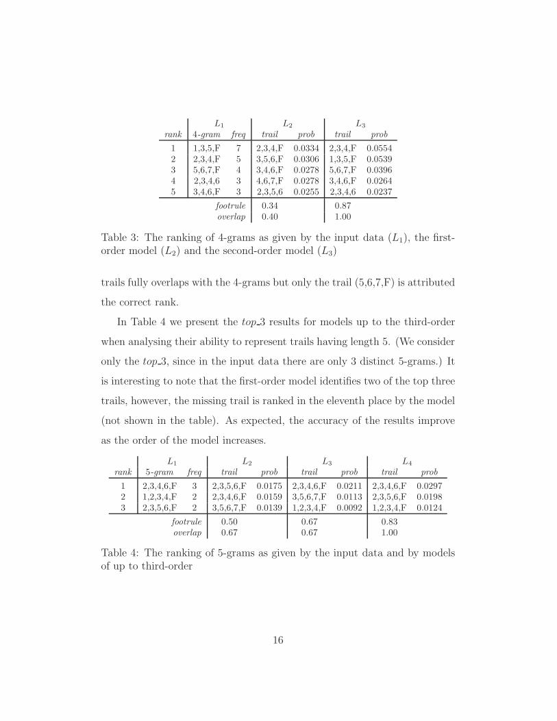
Table 3 presents the results of the analysis for trails having length 4. As

expected, the first-order model is less accurate for trails of length 4, and as

result we obtain a lower value for both the footrule metric and the overlap.

The first-order model is able to identify only 2 of the top 5 trails and is

not able to identify the most frequently traversed 4-gram. The second-order

15

L1 L2 L3

rank 4-gram freq trail prob trail prob

1 1,3,5,F 7 2,3,4,F 0.0334 2,3,4,F 0.05542 2,3,4,F 5 3,5,6,F 0.0306 1,3,5,F 0.05393 5,6,7,F 4 3,4,6,F 0.0278 5,6,7,F 0.03964 2,3,4,6 3 4,6,7,F 0.0278 3,4,6,F 0.02645 3,4,6,F 3 2,3,5,6 0.0255 2,3,4,6 0.0237

footrule 0.34 0.87overlap 0.40 1.00

Table 3: The ranking of 4-grams as given by the input data (L1), the first-order model (L2) and the second-order model (L3)

trails fully overlaps with the 4-grams but only the trail (5,6,7,F) is attributed

the correct rank.

In Table 4 we present the top 3 results for models up to the third-order

when analysing their ability to represent trails having length 5. (We consider

only the top 3, since in the input data there are only 3 distinct 5-grams.) It

is interesting to note that the first-order model identifies two of the top three

trails, however, the missing trail is ranked in the eleventh place by the model

(not shown in the table). As expected, the accuracy of the results improve

as the order of the model increases.

L1 L2 L3 L4

rank 5-gram freq trail prob trail prob trail prob

1 2,3,4,6,F 3 2,3,5,6,F 0.0175 2,3,4,6,F 0.0211 2,3,4,6,F 0.02972 1,2,3,4,F 2 2,3,4,6,F 0.0159 3,5,6,7,F 0.0113 2,3,5,6,F 0.01983 2,3,5,6,F 2 3,5,6,7,F 0.0139 1,2,3,4,F 0.0092 1,2,3,4,F 0.0124

footrule 0.50 0.67 0.83overlap 0.67 0.67 1.00

Table 4: The ranking of 5-grams as given by the input data and by modelsof up to third-order

16

2.4 Evaluation of the Predictive Power of a Model

In previous work we have presented a study focused on evaluating a model’s

ability to predict the last page of a session based on the preceding sequence

of pages viewed, [BL06]. We will now introduce this method.

To assess a model’s prediction ability we randomly split the set of input

trails into a training set and a test set, and then induce the model from the

training set. For each test trail of length l we use its l − 1 prefix to predict

the last page in the trail, which we call the prediction target (tg). The model

induced from the training set gives the set of reachable pages (rp) from the

tip of the prefix, assuming that the user has followed the sequence of pages

defined by the prefix. The reachable pages are ranked by probability, with

the most probable page having rank = 1. In order to measure the prediction

accuracy of the model, we let the Absolute Error (AE) measure the prediction

strength by setting AE = rank−1, i.e. the closer AE is to zero the better the

prediction is. The overall prediction accuracy metric is given by the Mean

Absolute Error (MAE) which is defined as the sum of AE over all the test

trails divided by the number of test trails.

We illustrate the method by assuming that the input trails given in Fig-

ure 1 (a) constitute the training set and that we have a test set composed

of the following three trails {(1, 3, 5) , (2, 3, 5, 6) , (1, 3, 5, 6, 7)}. According to

the first-order model after following the prefix (1,3) there are three reachable

pages (see Figure 1 (b)), the pages corresponding to states 4, 5 and F (the

latter corresponds to terminating the navigation session). In this case, the

prediction target (state 5) has rank 2 among the reachable pages resulting

in an absolute error AE=2-1=1. According to the second-order model (see

17

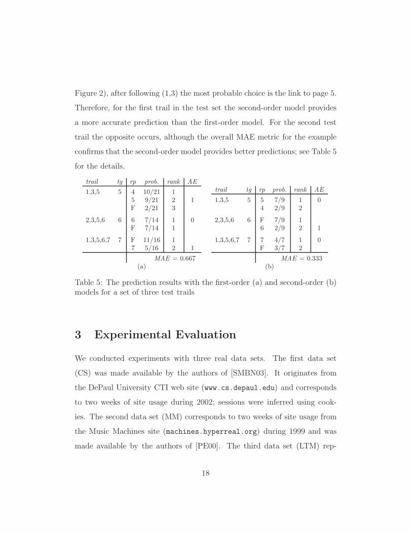
Figure 2), after following (1,3) the most probable choice is the link to page 5.

Therefore, for the first trail in the test set the second-order model provides

a more accurate prediction than the first-order model. For the second test

trail the opposite occurs, although the overall MAE metric for the example

confirms that the second-order model provides better predictions; see Table 5

for the details.

trail tg rp prob. rank AE

1,3,5 5 4 10/21 15 9/21 2 1F 2/21 3

2,3,5,6 6 6 7/14 1 0F 7/14 1

1,3,5,6,7 7 F 11/16 17 5/16 2 1

MAE = 0.667(a)

trail tg rp prob. rank AE

1,3,5 5 5 7/9 1 04 2/9 2

2,3,5,6 6 F 7/9 16 2/9 2 1

1,3,5,6,7 7 7 4/7 1 0F 3/7 2

MAE = 0.333(b)

Table 5: The prediction results with the first-order (a) and second-order (b)models for a set of three test trails

3 Experimental Evaluation

We conducted experiments with three real data sets. The first data set

(CS) was made available by the authors of [SMBN03]. It originates from

the DePaul University CTI web site (www.cs.depaul.edu) and corresponds

to two weeks of site usage during 2002; sessions were inferred using cook-

ies. The second data set (MM) corresponds to two weeks of site usage from

the Music Machines site (machines.hyperreal.org) during 1999 and was

made available by the authors of [PE00]. The third data set (LTM) rep-

18

resents a month of site usage from the London Transport Museum web site

(www.ltmuseum.co.uk) during January 2003. In the CS data set the sessions

were already identified, and for the other two data sets a session was defined

as a sequence of requests from the same IP address with a time limit of 30

minutes between consecutive requests. Erroneous and image requests were

eliminated from the data sets, although for the MM data set .jpg requests

were left in, since in that specific site they correspond to page views. When

preprocessing the data sets we set a session length limit of 15 requests, and,

therefore, very long sessions were split into two or more shorter sessions.

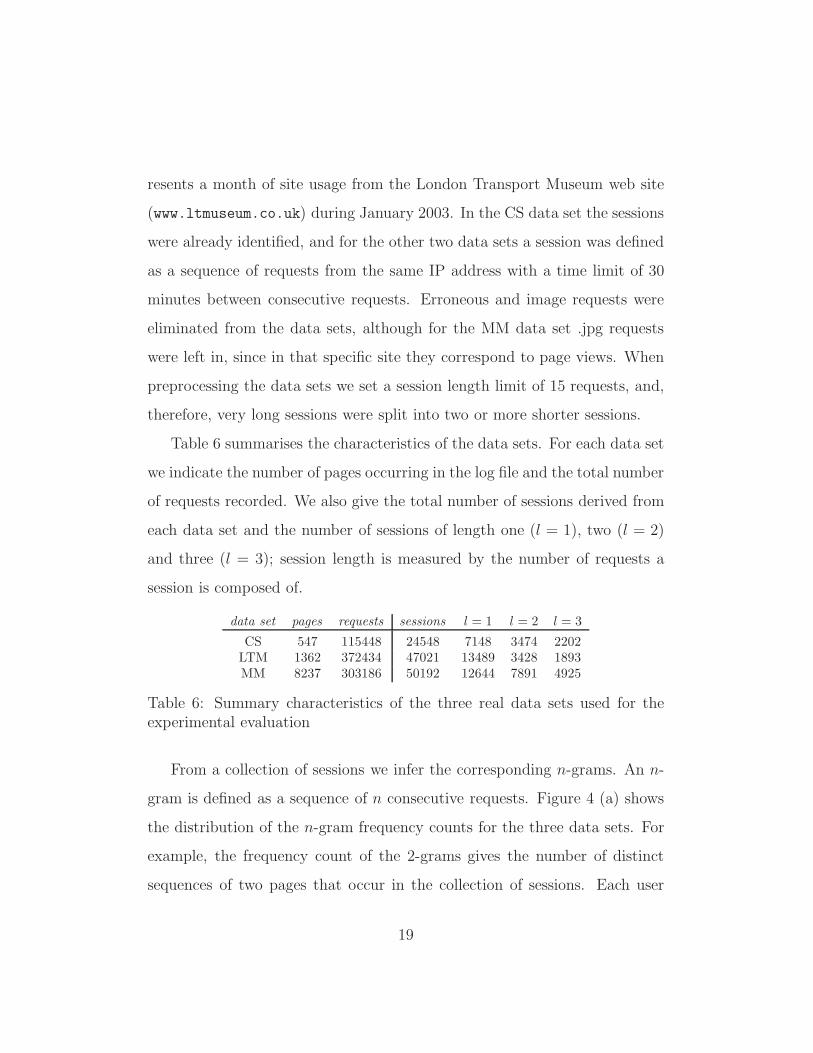
Table 6 summarises the characteristics of the data sets. For each data set

we indicate the number of pages occurring in the log file and the total number

of requests recorded. We also give the total number of sessions derived from

each data set and the number of sessions of length one (l = 1), two (l = 2)

and three (l = 3); session length is measured by the number of requests a

session is composed of.

data set pages requests sessions l = 1 l = 2 l = 3

CS 547 115448 24548 7148 3474 2202LTM 1362 372434 47021 13489 3428 1893MM 8237 303186 50192 12644 7891 4925

Table 6: Summary characteristics of the three real data sets used for theexperimental evaluation

From a collection of sessions we infer the corresponding n-grams. An n-

gram is defined as a sequence of n consecutive requests. Figure 4 (a) shows

the distribution of the n-gram frequency counts for the three data sets. For

example, the frequency count of the 2-grams gives the number of distinct

sequences of two pages that occur in the collection of sessions. Each user

19

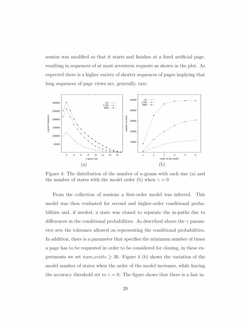
session was modified so that it starts and finishes at a fixed artificial page,

resulting in sequences of at most seventeen requests as shown in the plot. As

expected there is a higher variety of shorter sequences of pages implying that

long sequences of page views are, generally, rare.

300000

250000

200000

150000

100000

50000

161412108642

n-g

ram

fre

quen

cy

n-gram size

CSLTMMM

(a)

50000

40000

30000

20000

10000

654321

num

ber

of s

tate

s

order of the model

CSLTMMM

(b)

Figure 4: The distribution of the number of n-grams with each size (a) andthe number of states with the model order (b) when γ = 0

From the collection of sessions a first-order model was inferred. This

model was then evaluated for second and higher-order conditional proba-

bilities and, if needed, a state was cloned to separate the in-paths due to

differences in the conditional probabilities. As described above the γ param-

eter sets the tolerance allowed on representing the conditional probabilities.

In addition, there is a parameter that specifies the minimum number of times

a page has to be requested in order to be considered for cloning, in these ex-

periments we set num visits ≥ 30. Figure 4 (b) shows the variation of the

model number of states when the order of the model increases, while having

the accuracy threshold set to γ = 0. The figure shows that there is a fast in-

20

crease in the number of states for second and third order models. For higher

orders the number of states increases at a slower rate, which is an indication

that the gain in accuracy when using higher order models is smaller.

As discussed in Section 2.2, when γ = 0 a model of a given order ac-

curately represents trails of length ≤ order + 1 (the length of a trail is

measure by the number of pages views). For example, a first-order model ac-

curately represents the probability of a transition between any two states and

a second-order model accurately represents the probability of trails composed

of three consecutive states. In the following we make use of the method de-

scribed in Section 2.3 to assess the ability of a model to represent long trails.

Briefly, the method compares the ranking produced by the BFS algorithm

that infers the trails’ probability estimates with the ranking induced by the

n-gram frequency count. When the model is accurate the two resulting rank-

ings are identical.

For this purpose we consider three parameters: (i) the cut-point (λ),

i.e. only trails having probability above λ are considered, (ii) the maximum

length of a trail induced by the algorithm (mtl), and (iii) the size of the

ranked lists (top m). We consider two variations for the mtl parameter: (i) a

strict definition (mtl=) that takes into account only trails with the specified

length, and (ii) a non-strict definition (mtl<=) that takes into account trails

with length less than or equal to the specified limit. In (ii) we filter out sub-

trails, that is, trails that are a prefixes of longer trails whose probability is also

above the cut-point since, by definition of trail probability, all trail prefixes

have probability greater or equal to that of the full trail. As mentioned in

Section 2.3, in order to compare the rankings we make use of two metrics:

21

(i) overlap, and (ii) Spearman’s footrule metric. The overlap measures the

percentage of trails that occur in both rankings, while the footrule takes into

account not only the overlap but also the differences of rank ordering between

the lists. We note that although the cut-point is essential to reduce the search

space for the BFS algorithm, we will not emphasise it in our presentation,

since the mtl is the parameter that directly influences the top m ranking list.

In fact, the cut-point was necessary for large values of mtl due to the very

large number of trails to assess, however, its value did not have any impact

on the resulting top m ranking.

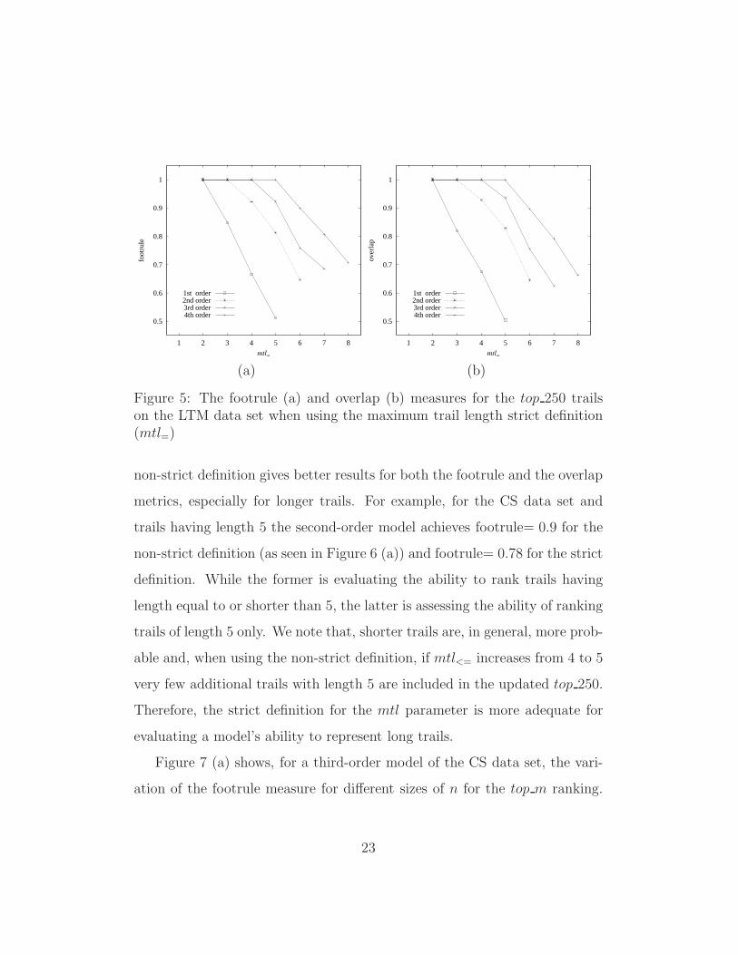
Figure 5 (a) shows, for the LTM data set, the footrule value for the

top 250 trails when using the strict trail length definition, mtl=. The results

show that a first-order model accurately ranks trails composed of one and

two requests. For trails of length three the value of the footrule is 0.85

revealing a close to linear decrease for longer trails. We point out that the

second-order model shows a footrule value of 0.92 for trails of length four.

Figure 5 (b) shows the overlap measure whose results are very similar to the

footrule metric. The overlap value shows a close to linear decrease as mtl=

increases. It is interesting to note that a first-order model achieves an overlap

of 0.50 for trails having length 5, which means that 50% of the top 250 trails

are identified in the list although probably not in the correct rank order. A

second-order model achieves an overlap of 0.64 for trails of length 6. Similar

results were obtained for the other two data sets.

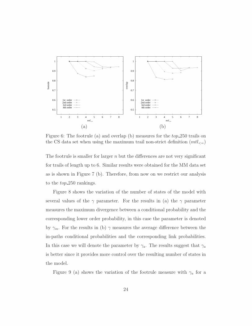
Figure 6 shows, for the CS data set, the results when the non-strict defi-

nition of the trail length limit parameter (mtl<=) is used. Again, the results

given by the footrule and overlap metrics are very similar. In general, the

22

1

0.9

0.8

0.7

0.6

0.5

87654321

foot

rule

mtl=

1st order2nd order3rd order4th order

(a)

1

0.9

0.8

0.7

0.6

0.5

87654321

over

lap

mtl=

1st order2nd order3rd order4th order

(b)

Figure 5: The footrule (a) and overlap (b) measures for the top 250 trailson the LTM data set when using the maximum trail length strict definition(mtl=)

non-strict definition gives better results for both the footrule and the overlap

metrics, especially for longer trails. For example, for the CS data set and

trails having length 5 the second-order model achieves footrule= 0.9 for the

non-strict definition (as seen in Figure 6 (a)) and footrule= 0.78 for the strict

definition. While the former is evaluating the ability to rank trails having

length equal to or shorter than 5, the latter is assessing the ability of ranking

trails of length 5 only. We note that, shorter trails are, in general, more prob-

able and, when using the non-strict definition, if mtl<= increases from 4 to 5

very few additional trails with length 5 are included in the updated top 250.

Therefore, the strict definition for the mtl parameter is more adequate for

evaluating a model’s ability to represent long trails.

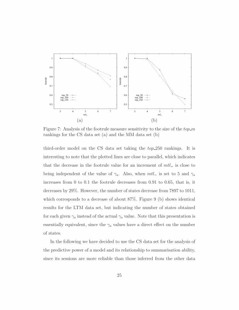
Figure 7 (a) shows, for a third-order model of the CS data set, the vari-

ation of the footrule measure for different sizes of n for the top m ranking.

23

1

0.9

0.8

0.7

0.6

0.5

87654321

foot

rule

mtl<=

1st order2nd order3rd order4th order

(a)

1

0.9

0.8

0.7

0.6

0.5

87654321

over

lap

mtl<=

1st order2nd order3rd order4th order

(b)

Figure 6: The footrule (a) and overlap (b) measures for the top 250 trails onthe CS data set when using the maximum trail non-strict definition (mtl<=)

The footrule is smaller for larger n but the differences are not very significant

for trails of length up to 6. Similar results were obtained for the MM data set

as is shown in Figure 7 (b). Therefore, from now on we restrict our analysis

to the top 250 rankings.

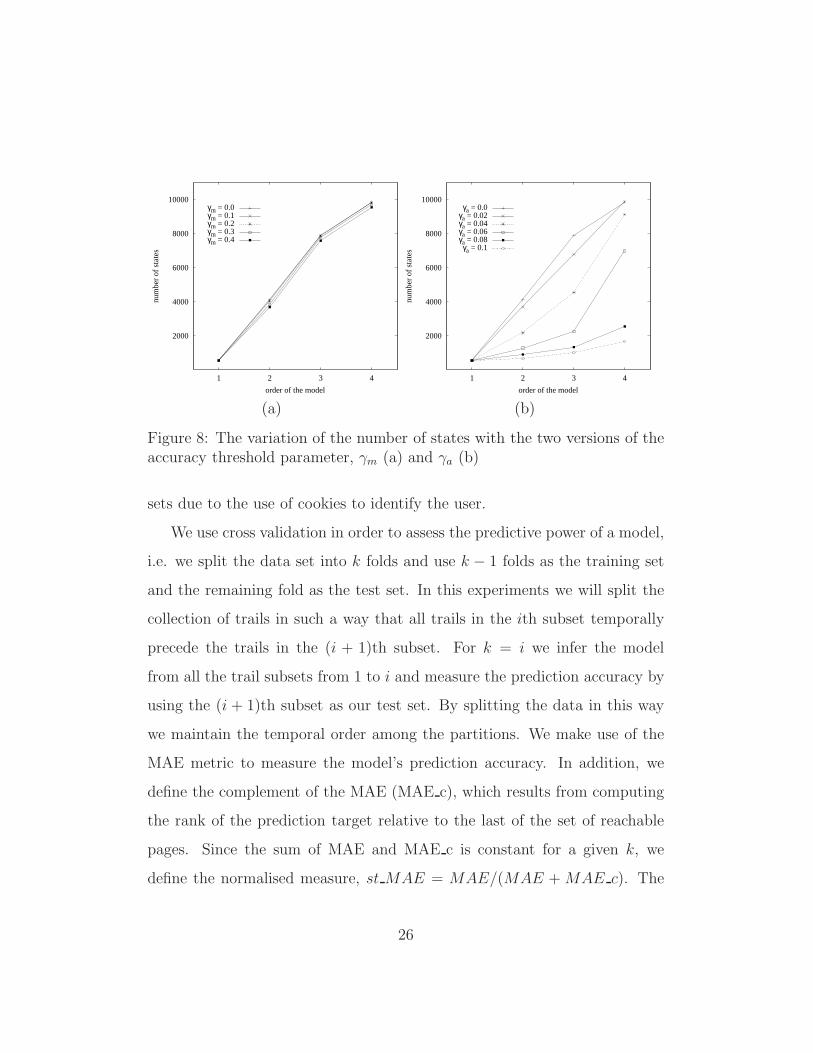
Figure 8 shows the variation of the number of states of the model with

several values of the γ parameter. For the results in (a) the γ parameter

measures the maximum divergence between a conditional probability and the

corresponding lower order probability, in this case the parameter is denoted

by γm. For the results in (b) γ measures the average difference between the

in-paths conditional probabilities and the corresponding link probabilities.

In this case we will denote the parameter by γa. The results suggest that γa

is better since it provides more control over the resulting number of states in

the model.

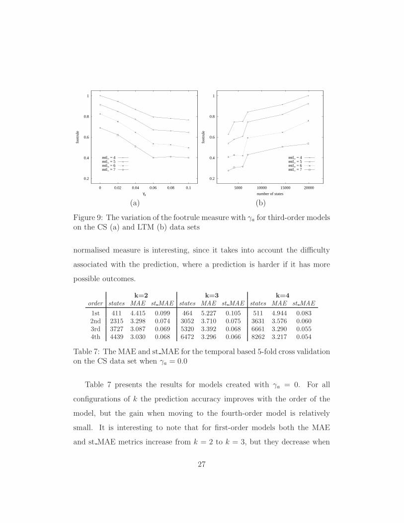
Figure 9 (a) shows the variation of the footrule measure with γa for a

24

1

0.9

0.8

0.7

0.6

0.5

76543

foo

trul

e

mtl=

top_50top_100top_250

(a)

0.5

0.6

0.7

0.8

0.9

1

76543

foot

rule

mtl=

top_50top_100top_250

(b)

Figure 7: Analysis of the footrule measure sensitivity to the size of the top mrankings for the CS data set (a) and the MM data set (b)

third-order model on the CS data set taking the top 250 rankings. It is

interesting to note that the plotted lines are close to parallel, which indicates

that the decrease in the footrule value for an increment of mtl= is close to

being independent of the value of γa. Also, when mtl= is set to 5 and γa

increases from 0 to 0.1 the footrule decreases from 0.91 to 0.65, that is, it

decreases by 29%. However, the number of states decrease from 7897 to 1011,

which corresponds to a decrease of about 87%. Figure 9 (b) shows identical

results for the LTM data set, but indicating the number of states obtained

for each given γa instead of the actual γa value. Note that this presentation is

essentially equivalent, since the γa values have a direct effect on the number

of states.

In the following we have decided to use the CS data set for the analysis of

the predictive power of a model and its relationship to summarisation ability,

since its sessions are more reliable than those inferred from the other data

25

10000

8000

6000

4000

2000

4321

num

ber

of s

tate

s

order of the model

γm = 0.0γm = 0.1γm = 0.2γm = 0.3γm = 0.4

(a)

10000

8000

6000

4000

2000

4321

num

ber

of s

tate

s

order of the model

γa = 0.0γa = 0.02γa = 0.04γa = 0.06γa = 0.08γa = 0.1

(b)

Figure 8: The variation of the number of states with the two versions of theaccuracy threshold parameter, γm (a) and γa (b)

sets due to the use of cookies to identify the user.

We use cross validation in order to assess the predictive power of a model,

i.e. we split the data set into k folds and use k − 1 folds as the training set

and the remaining fold as the test set. In this experiments we will split the

collection of trails in such a way that all trails in the ith subset temporally

precede the trails in the (i + 1)th subset. For k = i we infer the model

from all the trail subsets from 1 to i and measure the prediction accuracy by

using the (i + 1)th subset as our test set. By splitting the data in this way

we maintain the temporal order among the partitions. We make use of the

MAE metric to measure the model’s prediction accuracy. In addition, we

define the complement of the MAE (MAE c), which results from computing

the rank of the prediction target relative to the last of the set of reachable

pages. Since the sum of MAE and MAE c is constant for a given k, we

define the normalised measure, st MAE = MAE/(MAE + MAE c). The

26

1

0.8

0.6

0.4

0.2

0.10.080.060.040.020

foot

rule

γa

mtl= = 4mtl= = 5mtl= = 6mtl= = 7

(a)

1

0.8

0.6

0.4

0.2

2000015000100005000

foot

rule

number of states

mtl= = 4mtl= = 5mtl= = 6mtl= = 7

(b)

Figure 9: The variation of the footrule measure with γa for third-order modelson the CS (a) and LTM (b) data sets

normalised measure is interesting, since it takes into account the difficulty

associated with the prediction, where a prediction is harder if it has more

possible outcomes.

k=2 k=3 k=4

order states MAE st MAE states MAE st MAE states MAE st MAE

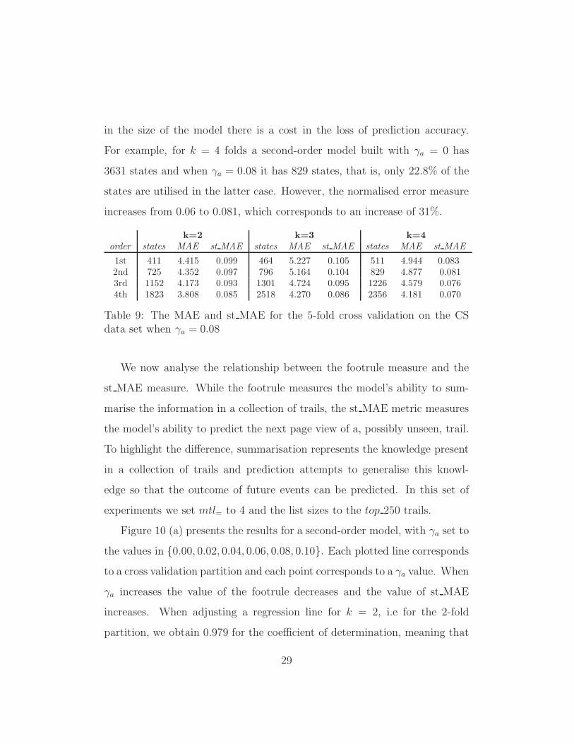
1st 411 4.415 0.099 464 5.227 0.105 511 4.944 0.0832nd 2315 3.298 0.074 3052 3.710 0.075 3631 3.576 0.0603rd 3727 3.087 0.069 5320 3.392 0.068 6661 3.290 0.0554th 4439 3.030 0.068 6472 3.296 0.066 8262 3.217 0.054

Table 7: The MAE and st MAE for the temporal based 5-fold cross validationon the CS data set when γa = 0.0

Table 7 presents the results for models created with γa = 0. For all

configurations of k the prediction accuracy improves with the order of the

model, but the gain when moving to the fourth-order model is relatively

small. It is interesting to note that for first-order models both the MAE

and st MAE metrics increase from k = 2 to k = 3, but they decrease when

27

states MAE st MAE

512 4.787 0.0814000 3.471 0.0599533 3.090 0.05213173 2.961 0.050

Table 8: The MAE and st MAE on the CS data set for the non-temporalbased 5-fold cross validation when γa = 0.0

moving to k = 4. We remind the reader that the higher k is the larger

the data set used to construct the model is, resulting in models with a larger

number of states (as can be verified in Table 7) on which predictions are more

difficult. Another aspect that should be taken into account is that when k

increases the sessions in the training set cover a larger period of time. For

example, for k = 4 we are training the model with data from four periods of

time and testing with the last period. In cases where the user’s behaviour

changes over time a model trained with data covering a larger period may

have problems in generalising for future user behaviour.

In Table 8 present the results obtained with the standard 5-fold cross val-

idation; we note that in [BL06] we used the standard cross validation rather

than the temporal-based version used herein. When comparing the results we

must take into account the fact that each value presented corresponds to the

average result for the 5 splits. Moreover, the number of states is larger than

that obtained from the temporal-based split, since we used num visits ≥ 15,

which leads to more states being cloned. However, overall, the results are

very similar to those obtained with the temporal-based cross validation.

Table 9 gives the results obtained when γa = 0.08. As expected, when

γa increases the accuracy of the conditional probabilities decreases but we

obtain models having a significantly smaller number of states. For a gain

28

in the size of the model there is a cost in the loss of prediction accuracy.

For example, for k = 4 folds a second-order model built with γa = 0 has

3631 states and when γa = 0.08 it has 829 states, that is, only 22.8% of the

states are utilised in the latter case. However, the normalised error measure

increases from 0.06 to 0.081, which corresponds to an increase of 31%.

k=2 k=3 k=4

order states MAE st MAE states MAE st MAE states MAE st MAE

1st 411 4.415 0.099 464 5.227 0.105 511 4.944 0.0832nd 725 4.352 0.097 796 5.164 0.104 829 4.877 0.0813rd 1152 4.173 0.093 1301 4.724 0.095 1226 4.579 0.0764th 1823 3.808 0.085 2518 4.270 0.086 2356 4.181 0.070

Table 9: The MAE and st MAE for the 5-fold cross validation on the CSdata set when γa = 0.08

We now analyse the relationship between the footrule measure and the

st MAE measure. While the footrule measures the model’s ability to sum-

marise the information in a collection of trails, the st MAE metric measures

the model’s ability to predict the next page view of a, possibly unseen, trail.

To highlight the difference, summarisation represents the knowledge present

in a collection of trails and prediction attempts to generalise this knowl-

edge so that the outcome of future events can be predicted. In this set of

experiments we set mtl= to 4 and the list sizes to the top 250 trails.

Figure 10 (a) presents the results for a second-order model, with γa set to

the values in {0.00, 0.02, 0.04, 0.06, 0.08, 0.10}. Each plotted line corresponds

to a cross validation partition and each point corresponds to a γa value. When

γa increases the value of the footrule decreases and the value of st MAE

increases. When adjusting a regression line for k = 2, i.e for the 2-fold

partition, we obtain 0.979 for the coefficient of determination, meaning that

29

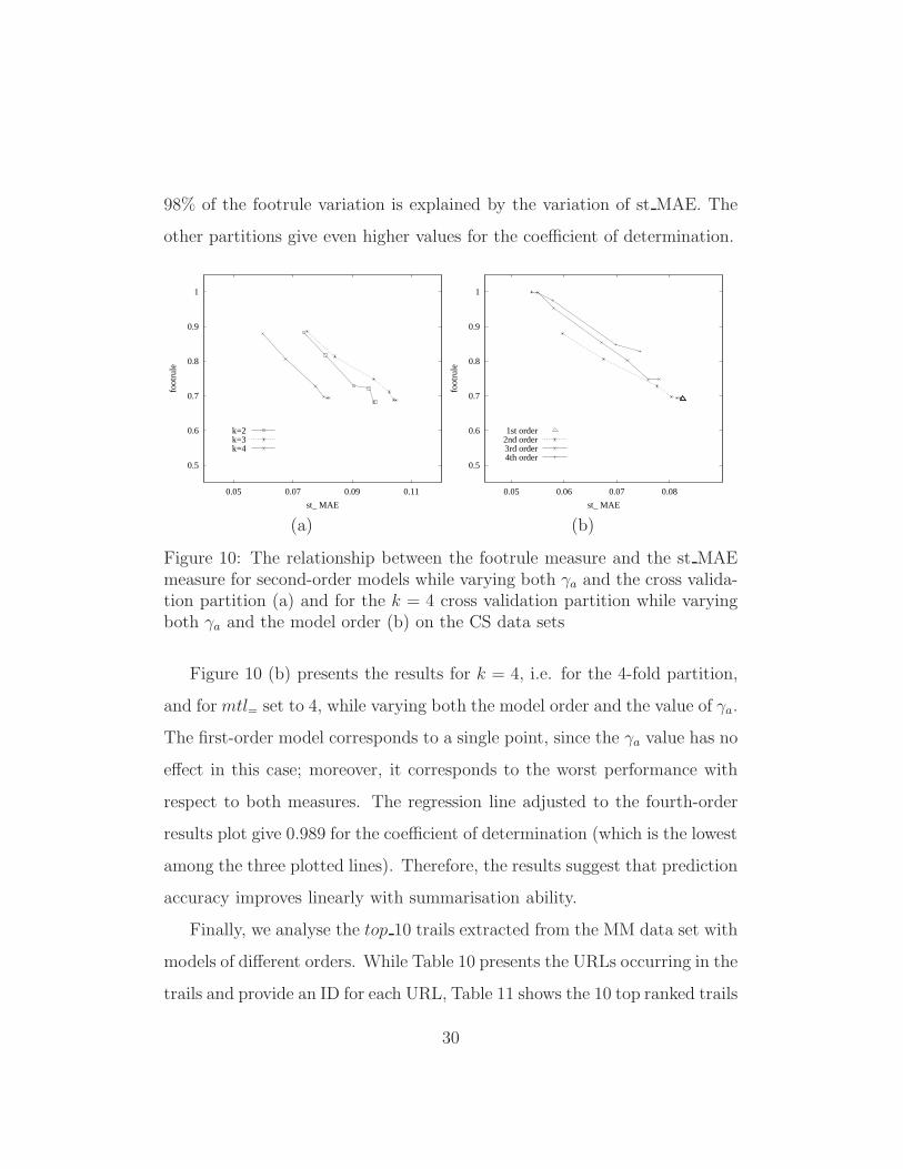
98% of the footrule variation is explained by the variation of st MAE. The

other partitions give even higher values for the coefficient of determination.

0.5

0.6

0.7

0.8

0.9

1

0.110.090.070.05

foot

rule

st_ MAE

k=2k=3k=4

(a)

0.5

0.6

0.7

0.8

0.9

1

0.080.070.060.05

foot

rule

st_ MAE

1st order2nd order3rd order4th order

(b)

Figure 10: The relationship between the footrule measure and the st MAEmeasure for second-order models while varying both γa and the cross valida-tion partition (a) and for the k = 4 cross validation partition while varyingboth γa and the model order (b) on the CS data sets

Figure 10 (b) presents the results for k = 4, i.e. for the 4-fold partition,

and for mtl= set to 4, while varying both the model order and the value of γa.

The first-order model corresponds to a single point, since the γa value has no

effect in this case; moreover, it corresponds to the worst performance with

respect to both measures. The regression line adjusted to the fourth-order

results plot give 0.989 for the coefficient of determination (which is the lowest

among the three plotted lines). Therefore, the results suggest that prediction

accuracy improves linearly with summarisation ability.

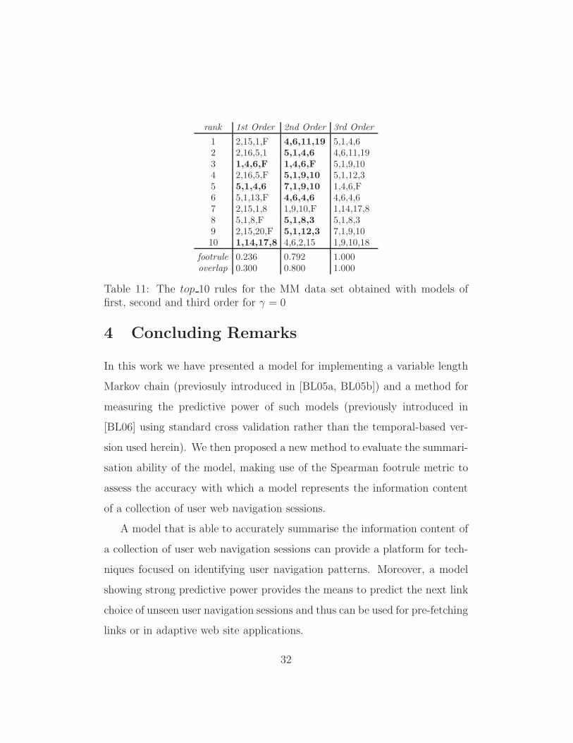
Finally, we analyse the top 10 trails extracted from the MM data set with

models of different orders. While Table 10 presents the URLs occurring in the

trails and provide an ID for each URL, Table 11 shows the 10 top ranked trails

30

having length four that are inferred from first, second and third-order models,

with γa = 0.0. The footrule and the overlap metrics are also indicated. As

expected the third-order model ranks accurately the trails of length four

and, we therefore use it as the reference ranking for the other models. The

first-order model is able to identify three of the top 10 trails although with

a different ranking. The second-order model is able to identify eight of the

top 10 trails. For lower order models the trails in bold were identified from

the reference ranking.

ID URL

1 /2 /music/machines/analogue-heaven3 /manufacturers/roland4 /music/machines/samples.html5 /music/machines6 /samples.html7 /machines8 /manufacturers9 /music/machines/categories/software/windows10 /categories/software/windows11 /music/machines/categories/drum-machines/samples12 /analogue-heaven13 /search.cgi14 /guide15 /analogue-heaven16 /music/machines/images/farley3.jpg17 /guide/finding.html18 /categories/software/windows/readme19 /categories/drum-machines/samples20 /analogue-heaven/email.html

Table 10: The URLs occurring in the rules given in Table 11

31

rank 1st Order 2nd Order 3rd Order

1 2,15,1,F 4,6,11,19 5,1,4,62 2,16,5,1 5,1,4,6 4,6,11,193 1,4,6,F 1,4,6,F 5,1,9,104 2,16,5,F 5,1,9,10 5,1,12,35 5,1,4,6 7,1,9,10 1,4,6,F6 5,1,13,F 4,6,4,6 4,6,4,67 2,15,1,8 1,9,10,F 1,14,17,88 5,1,8,F 5,1,8,3 5,1,8,39 2,15,20,F 5,1,12,3 7,1,9,1010 1,14,17,8 4,6,2,15 1,9,10,18

footrule 0.236 0.792 1.000overlap 0.300 0.800 1.000

Table 11: The top 10 rules for the MM data set obtained with models offirst, second and third order for γ = 0

4 Concluding Remarks

In this work we have presented a model for implementing a variable length

Markov chain (previosuly introduced in [BL05a, BL05b]) and a method for

measuring the predictive power of such models (previously introduced in

[BL06] using standard cross validation rather than the temporal-based ver-

sion used herein). We then proposed a new method to evaluate the summari-

sation ability of the model, making use of the Spearman footrule metric to

assess the accuracy with which a model represents the information content

of a collection of user web navigation sessions.

A model that is able to accurately summarise the information content of

a collection of user web navigation sessions can provide a platform for tech-

niques focused on identifying user navigation patterns. Moreover, a model

showing strong predictive power provides the means to predict the next link

choice of unseen user navigation sessions and thus can be used for pre-fetching

links or in adaptive web site applications.

32

We presented the results of an extensive experimental evaluation con-

ducted on three real world data sets, which provide strong evidence that

their is a linear relationship between predictive power and summarisation

ability.

As future work, we are planning to incorporate our model within an

adaptive web site platform in order to assess it as an online tool to provide

link suggestions for users navigating within a site.

References

[Bej04] G. Bejerano. Algorithms for variable length Markov chain mod-

elling. Bioinformatics, 20:788–789, March 2004.

[BL00] J. Borges and M. Levene. Data mining of user navigation pat-

terns. In B. Masand and M. Spiliopoulou, editors, Web Usage

Analysis and User Profiling, Lecture Notes in Artificial Intelli-

gence (LNAI 1836), pages 92–111. Springer-Verlag, Berlin, 2000.

[BL04] J. Borges and M. Levene. An average linear time algorithm for

web usage mining. International Journal of Information Technol-

ogy and Decision Making, 3(2):307–319, June 2004.

[BL05a] J. Borges and M. Levene. A clustering-based approach for mod-

elling user navigation with increased accuracy. In Proceedings of

the 2nd International Workshop on Knowledge Discovery from

Data Streams, pages 77–86, Porto, Portugal, October 2005.

33

[BL05b] J. Borges and M. Levene. Generating dynamic higher-order

markov models in web usage mining. In A. Jorge, L. Torgo,

P. Brazdil, R. Camacho, and J. Gama, editors, Proceedings of the

9th European Conference on Principles and Practice of Knowl-

edge Discovery in Databases (PKDD), Lecture Notes in Artificial

Intelligence (LNAI 3271), pages 34–45, Porto, Portugal, October

2005. Springer-Verlag.

[BL06] J. Borges and M. Levene. Testing the predictive power of vari-

able history web usage. To appear in Journal of Soft Computing,

Special Issue on Web Intelligence, 2006.

[CZ03] X. Chen and X. Zhang. A popularity-based prediction model for

web prefetching. IEEE Computer, pages 63–70, 2003.

[DJ02] X. Dongshan and S. Juni. A new Markov model for web access

prediction. IEEE Computing in Science & Engineering, 4:34–39,

November 2002.

[DK04] M. Deshpande and G. Karypis. Selective Markov models for pre-

dicting web page accesses. ACM Transactions on Internet Tech-

nology, 4:163–184, May 2004.

[EVK05] M. Eirinaki, M. Vazirgiannis, and D. Kapogiannis. Web path

recommendations based on page ranking and Markov models. In

WIDM ’05: Proceedings of the 7th annual ACM international

workshop on Web information and data management, pages 2–9,

New York, NY, USA, 2005. ACM Press.

34

[FKS03] R. Fagin, R. Kumar, and D. Sivakumar. Comparing top k lists.

SIAM Journal of Discrete Mathematics, 17(1):134–160, Novem-

ber 2003.

[JPT03] S. Jespersen, T.B. Pedersen, and J. Thorhauge. Evaluating the

markov assumption for web usage mining. In Proceedings of the

fifth ACM international workshop on Web information and data

management, pages 82–89, 2003.

[Mob04] B. Mobasher. Web usage mining and personalization. In Munin-

dar P. Singh, editor, Practical Handbook of Internet Computing.

Chapman Hall & CRC Press, Baton Rouge, 2004.

[PE00] M. Perkowitz and O. Etzioni. Towards adaptive web sites:

Conceptual framework and case study. Artificial Intelligence,

118(2000):245–275, 2000.

[SKS98] S. Schechter, M. Krishnan, and M.D. Smith. Using path pro-

files to predict HTTP requests. Computer Networks and ISDN

Systems, 30:457–467, 1998.

[SMBN03] M. Spiliopoulou, B. Mobasher, B. Berendt, and M. Nakagawa.

A framework for the evaluation of session reconstruction heuris-

tics in web usage analysis. IN-FORMS Journal on Computing,

(15):171–190, 2003.

35