1

Evaluating Implied Cost of Capital Estimates

By

Charles M. C. Lee**

Eric C. So

Charles C.Y. Wang

Preliminary Draft

April 8th, 2010

Abstract We propose a two-dimensional evaluation scheme for assessing the quality of implied cost of capital (ICC) estimates when price is noisy. Under fairly general assumptions, high-quality ICC estimates should: (a) better forecast future realized returns, and (b) better forecast future ICCs. Empirically, we compare seven alternative ICC estimates and show that several perform well along both dimensions. Moreover, we find that the lagged industry median ICC computed using any of the successful models will predict both future firm-level returns and firm-level ICCs. These results offer support for a parsimonious industry-based ICC estimate in investment or capital budgeting decisions.

** All three authors are at Stanford University. Lee (professor.lee@gmail.com) is the Joseph McDonald Professor of Accounting at the Stanford Graduate School of Business (GSB); So (eso@stanford.edu) is a Doctoral Candidate in Accounting at the Stanford GSB; Wang (charles.cy.wang@stanford.edu) is a Doctoral Candidate in the Department of Economics. We thank seminar participants at the Stanford Accounting Research workshop for helpful comments and suggestions.

2

I. Introduction The implied cost of capital (ICC) for a given asset can be defined as the discount rate (or internal rate of return) that equates the asset’s market value to the present value of its expected future cash flows. In recent years, a substantial literature on ICCs has developed, first in accounting, and now increasingly, in finance. The collective evidence from these studies indicates that the ICC approach offers significant promise in dealing with a number of long-standing empirical asset pricing conundrums.1 The emergence of this literature is, in large part, attributable to the failure of the standard asset pricing models to provide precise estimates of the firm-level cost of equity capital.2 An important appeal of the ICC as a proxy for expected returns is that it does not rely on noisy realized asset returns. At the same time, the use of ICC as a proxy for expected returns is not without its own problems and limitations. In this study, we address a recurrent problem that seems to stand in the way of broader adoption of ICCs as proxies for firm-level expected returns – that of performance evaluation. Specifically, when prices (and therefore realized returns) are noisy, how can we assess the quality/validity of alternative firm-level ICC estimates? What are appropriate performance benchmarks? In other words, how do we know when we have a good ICC estimate? The importance of this problem is highlighted by the myriad of (seemingly arbitrary) assumptions and valuation approaches used to forecast firm-level cash flows. At a minimum, sensible ICC estimates call for sensible cash flow forecasts. But an endless combination of apparently equally defensible forecasting assumptions can be made, each of which can lead to a different set of ICC estimates. When do these differences matter? How might we adjudicate between them? More importantly, will our failure to do so detract from the credibility of the entire approach? 1 See Easton (2007) for a summary of the accounting literature prior to 2007. In finance, the ICC methodology has been used to test the Intertemporal CAPM (Pastor et al. (2008)), international asset pricing models (Lee et al. (2009)), and default risk (Chava and Purnanadam (2009)). In each case, the ICC approach has provided new evidence on the risk:return relation that is more intuitive and more consistent with theoretical predictions than those obtained using ex post realized returns. 2 The problems with using ex post realized returns to proxy for expected returns are well documented (e.g., see Fama and French (1997), Elton (1999), and Pastor and Stambaugh (1999)). In their concluding remarks, Fama and French (1997) write: “Estimates of the cost of equity are distressingly imprecise… (O)ur message is that the task is beset with massive uncertainty… whatever the formal approach two of the ubiquitous tools in capital budgeting are a wing and a prayer, and serendipity is an important force in outcomes.” (page 178-179)

3

We derive key properties of expected return proxies based on minimalistic assumptions about the price formation process. Using this framework, we propose a two-dimensional evaluation scheme for assessing the quality of implied cost of capital (ICC) estimates when price is noisy. Specifically, we show that, under fairly general assumptions, high-quality ICC estimates should both: (a) better forecast future realized returns (exhibit “predictability”), and (b) better forecast future ICCs (exhibit good “tracking”).3 Our analyses show that firms’ true, but unobservable, expected returns possess both these qualities, and when measurement errors in ICC estimates are small or “well-behaved” (see Section II), the ICC estimates also exhibit these qualities. Prior studies that tackle the performance evaluation issue have resorted to one of two approaches: (a) by comparing the ICC estimates’ correlation with realized ex post returns, or (b) by comparing the ICC estimates’ correlation with perceived risk proxies, such as beta, leverage, B/M, volatility, or size. In the first approach, ICCs that are more correlated with future realized returns (raw or corrected) are deemed to be of higher validity (e.g. Guay et al. (2005) and Easton and Monahan (2005)).4 In the second approach, ICCs that exhibit more positive (i.e., a more “stable and meaningful”) correlation with the other risk proxies are deemed to be superior (Botosan and Plumlee (2005)). Although both approaches have some merit, neither weans us fully from the problems that gave rise to the need for ICCs in the first place (i.e. noisy prices and the poor performance of other risk proxies). Perhaps more importantly, these prior studies offer no measurable assurance that the ICC estimates are at all useful for their intended purpose. For example, after examining seven ICC estimates, Easton and Monahan (2005) [EM] concluded that “for the entire cross-section of firms, these proxies are unreliable. None of them has a positive association with realized returns, even after controlling for the bias and noise in realized returns…” (page 501) Using the dual criteria of predictive power and tracking ability, we empirically assess the usefulness of seven different ICC estimates. Four of these ICC

3 Our approach is similar to the two-dimensional performance metrics used by Lee, Myers and Swaminathan (1999) [LMS] to compare alternative value estimates for the Dow30 stocks. However, whereas LMS is focused on evaluating alternative value estimates in a univariate time-series, we compare the relative performance of ICC estimates in a cross-sectional context. 4 Guay et al. (2005) examines the correlation between alternative ICC estimates and raw ex post returns. Easton and Monahan (2005)[EM] introduces a method for purging these returns of the estimated effect of future news. We discuss the EM approach in much more detail later.

4

estimates are based on an earnings capitalization model (PEG, MPEG, OJM, and AGR), one is based on a residual-income model (GLS), and two are based on a Gordon Growth Model (EPR, GGM). To avoid potential problems associated with analyst earning forecasts, and to ensure the largest possible sample, we use the cross-sectional technique introduced by Hou et al. (2009) to forecast future earnings. Our sample consists of 11,981 unique firms (80,902 firm-years) spanning the 1971-2007 time-period. We find that four of these estimates (GLS, GGM, EPR, and AGR) have a statistically reliable correlation with future realized returns over the next 12 to 60 months, while three others (OJM, PEG, MPEG) do not. Among the four proxies with some predictive power, GLS and GGM seem to offer appreciably better tracking ability. Further analyses using a GGM model with varying forecast horizons (one-year through five-year) show that as the forecasting horizon is lengthened, we gain tracking ability at a slight loss of predictive power. Moreover, we show that a simple industry-based ICC estimate based on any of the four successful estimation models (GLS, GGM, EPR, or AGR) will reliably capture a significant amount of cross-sectional variation in future firm-level realized returns (i.e., has good firm-level predictive power), while also exhibiting a significant ability to predict future firm-level ICCs (i.e., good firm-level tracking ability). These results provide support for the use of an industry-based ICC estimate in investment or capital budgeting decisions. For illustration, we provide a simple case study of how this method can be used in a classroom setting. Collectively, our results offer a much more sanguine assessment of ICC estimates than some of the prior literature. Our analyses indicate that the EM conclusion is likely due to the noisy nature of the filter they applied to ex post realized returns, and is not an indictment of the ICC methodology. At the same time, our results help to reconcile academic findings with financial practice, which often implicitly employs industry-based ICC corrections for equity valuation purposes. The rest of the paper is organized as follows. In Section II, we develop the theoretical underpinnings for our performance metrics. In Section III we discuss Data and Sample issues, explain our research design, and review the construction of our seven ICC estimates. Section IV contains our empirical results, and Section V concludes.

5

II. Theoretical Underpinnings II.1 Return Decomposition Revisited A firm’s returns in period t+1 may be thought of as consisting of an expected component and an unexpected component. Formally:

,1,1,1, titi

erti

r (1)

where ri, t+1 is the realized return for firm i in period t+1, eri, t+1 is expected return at the

beginning of t+1 conditional on available information, and i, t+1 is unexpected return. One way to parse unexpected return is to decompose it into two components, relating to cash flow news (i.e. shocks to expected cash flows) and discount rates news (i.e. shocks to discount rates). Campbell (1991) and Campbell and Shiller (1988a, 1988b) adopt this approach for their analysis of aggregate market returns, and Vuolteenaho (2002) extended it to a firm-level analysis:

1,1,1,1, ti

rnti

cfnti

erti

r , (2)

where cfni,t+1 is cash flow news in period t+1 and rni, t+1 is discount rate news in period t+1. This is the framework adopted by Easton and Monahan (2005) to test the validity/quality of ICC estimates. Reasoning that the bias and noise in realized returns can be removed (or at least reduced) by controlling for cash flow and discount rate news, EM attempt to estimate empirical proxies for cfn and rn. Alternative ICC estimates are then evaluated in terms of their association with the “corrected” realized return measure. Notice that this decomposition is based on a strong assumption about the source of stock return movements. Specifically, it assumes that Pt = Vt for all t, where Pt is price and Vt

is the present value of its expected future cash payoffs to shareholders. In other words, this decomposition does not entertain the possibility that prices move for any reason other than fundamental news. It does not consider market mispricing of any kind, whether from model uncertainty (e.g. Pastor and Stambaugh (1999)), investor sentiment ((Shiller (1984), De Long et al. (1990), Cutler et al. (1989)), or any other sources of noise ((Roll

6

(1984), Black (1986)). This is a strong assumption, even for adherents of competitively efficient markets.5 The assumption of price:value equivalence might not be a serious problem in the original context in which it appeared. For example, Campbell (1991) and Vuolteenaho (2002) use this decomposition to infer the relative importance of cash flow news and discount rate news in explaining overall return volatility (i.e., the framework is used primarily for a variance decomposition analysis). However, the application of this framework to the testing of firm-level ICC estimates can be much more problematic. In fact, by assuming that stock returns always reflect fundamental news, we may well have assumed away the problems that gave rise to the need for ICCs in the first place. II.2 An Alternative Approach Now consider a slightly different return decomposition. Using similar notation, we can express a stock’s realized return as: (3)

where ri,t+1 is the realized return for firm i in period t+1, and eri,t+1 is its expected return at the beginning of the period. As before, rni,t+1 is discount rate news (i.e., rni,t+1 reflects innovations that revise the market’s expectation of stock i’s future return). The last term, uni,t+1 , captures all other innovations or shocks to price that are not ex ante forecastable. Note that in the special case where all other shocks to price are due to cash flow news, equation (3) is identical to equation (2). However, in our framework, the unforecastable component of realized return is a much broader concept, and need not be related to cash flow news. Next, we make the assumption that firm-level news is truly white noise. In other words, firm-specific innovations in each period sum to zero in expectation, and are unrelated to expected returns. Formally:

01,1,

tirnE

tiunE tt

, and (A1)

01,

,1,1,

,1,

tirn

tierCov

tiun

tierCov (A2)

5 In fact, as Shiller (1987; page 458-459) famously observed, this assumption need not hold even if markets are competitively efficient (i.e. even if returns cannot be easily forecasted, prices can still be substantially different from their fundamental values).

1,1,1,1, tiun

tirn

tier

tir

7

Given (A1), it is fairly straightforward to show that expected returns, in the cross section, should forecast realized returns. In addition, given (A2), cross-sectional expected returns should also track itself – that is, true expected return should be “sticky” in the cross-section, so that high expected return firms in one period should on average have high expected return in the next period. We demonstrate these two intuitive cross-sectional properties of expected returns more formally below:

1. Predictability Because idiosyncratic noise can be largely diversified away, a portfolio’s realized return should be a good estimate of the average expected return of the individual stocks. That is:

N

i

N

i

N

i

N

i tiun

Ntirn

Ntier

Ntir

N 1111 1,1

1,1

1,1

1,1 (4)

Given a sufficiently large number of stocks (and remembering that er is the true expected return), the last two terms in equation (4) are zero in expectation. Notice that this result follows directly from (A1).

2. Tracking The cross-sectional relation between this period’s expected returns and next period’s expected returns is also intuitive: on average, this period’s expected return is an unbiased forecast of next period’s expected return: To show this, note that: 1,1,2, tirntiertier (5)

If we conduct a cross-sectional regression of eri,t+2 on eri,t+1, the estimated slope coefficient is:

1

1,

1,,

1,1,

1,

1,,

2,ˆLLN

tierVar

tier

tirn

tierCov

tierVar

tier

tierCov

(6)

By the Law of Large Numbers (LLN), the estimated slope coefficient approaches 1 for a sufficiently large number of stocks. This result follows directly from (A2).

8

Because rni,t+1 is unforecastable, it is by definition uncorrelated with expected returns.

In short, under fairly general assumptions, true cross-sectional expected returns will: (a) predict future realized returns, and (b) track future expected returns. However, because expected returns are not observable, we now turn to the empirical proxies of expected returns (ICC’s). We can model estimated ICC’s as the true expectation, measured with error: 1,1,1,ˆ tititi erre , (7)

where i,t+1 represents the measurement error for firm i in period t+1. Note that the differences between alternative ICC estimates will be reflected in the properties (time-

series and cross-sectional) of their terms. In this section, we develop a set of three, progressively weaker, assumptions under which estimated ICCs will continue to exhibit both predictability for future returns and tracking ability for future ICC estimates:

1) Measurement errors are small at all times (i.e. i,t+1~0 for all i and all t). Here the intuition is straightforward. If we measure expected returns with little or no error, predictability and tracking of ICC follows immediately from above results.

2) Measurement errors exist, but are ‘white noise’. By this we mean that (a) the average expected measurement error across a sufficiently large number of firms, is zero (i.e.,

E(i,t+1) = 0), and (b) the measurement errors are uncorrelated with the level of ICC. This is a less restrictive assumption than 1). Under this assumption, we can obtain predictability of realized returns using ICCs, in the sense of equation (4). To show this, recall from equation (4):

0)(0

11

0

1

0

111

1,1

1,ˆ

1

1,1

1,1

1,1

1,1

underELLNby

N

i

N

i

LLNby

N

i

LLNby

N

i

N

i

N

i

tiNtire

N

tirn

Ntiun

Ntier

Ntir

N (8)

9

In addition, we can demonstrate that ICC estimates will exhibit tracking. Here, we write the relation between ICC from one period to the next as:

(9)

Then, for an ICC estimate, the cross-sectional regression of one period’s ICC to last period’s will yield: (10)

This result follows directly from the fact that measurement errors (both in the current and subsequent period), as well as the unexpected discount rate news, are uncorrelated with the ICC estimates.

3) Measurement errors are systematic, but error reversions are uncorrelated with ICCs

(i.e. E(i,t+1) =K for some constant K; but Cov (i,t+2 - i,t+1, 1,ˆ tire ) =0).

Although ICC estimates are biased in the cross-section, the error reversions are not systematically related to the ICC estimate itself. In this case, we can obtain predictability in the cross-section, but our estimates of realized returns will be off by a constant (K). Although we cannot observe K, we can remove its effect by computing individual ICC estimates relative to an overall market ICC. The intuition is that so long as biases produced by ICCs are systematic and predictable, we can undo such biases to back out the correct measurement of expected returns.6 That is,

K

N

i

N

i

LLNby

N

i

LLNby

N

i

N

i

N

i

tiNtire

N

tirn

Ntiun

Ntier

Ntir

N

11

0

1

0

111

1,1

1,ˆ

1

1,1

1,1

1,1

1,1

(11)

6 Such systematic biases would also be removed when considering the hedge returns from a long-short portfolio.

1,1,1,ˆ

2,2,ˆ

tirn

titire

titire

1

1,ˆ

1,ˆ,

1,2,1,1,ˆ

1,ˆ

1,ˆ,

2,ˆ

ˆLLN

tireVar

tire

tirn

tititireCov

tireVar

tire

tireCov

10

Note that under such a framework we can also achieve tracking – this property follows directly from the fact that the reversion speed is uncorrelated with the ICC.7

To summarize, the above analyses suggest two dimensions along which we can evaluate alternative ICC estimates: cross-sectional return predictability and tracking. Under fairly general assumptions, good ICC estimates should exhibit both characteristics. Note that these two performance criteria correspond reasonably well to two realistic decision contexts often encountered by investment professionals. On the one hand, investors are interested in knowing how well today’s ICC estimates predict future stock returns – i.e., on average, expected returns and realized returns should be positively correlated in the cross-section. On the other hand, investors are also interested in how well today’s ICC estimates predict future ICC estimates (i.e., how well will today’s market multiple for a particular firm predict its future market multiple). In the following section we apply this evaluation framework to assess the merits of seven alternative ICC measures. III. Research Methodology III.1: Data and Sample Selection We obtain market-related data on all U.S.-listed firms (excluding ADRs) from CRSP, and annual accounting data from Compustat. To be included, each firm-year observation must have information on stock price, shares outstanding, book values, earnings, dividends, and industry identification (SIC codes). We also require sufficient data to calculate forecasts of future earnings based on the methodology outlined in Hou et al (2009), and to estimate ICCs for all seven models. Our final sample consists of 80,902 firm-years and 11,981 unique firms, spanning 1970-2007 (see Appendix I). Note that this sample is considerably larger than those used in most prior ICC studies that require I/B/E/S analyst forecasts. III.2: Earnings Forecasts In a recent study, Hou et al. (2009) use a pooled cross-sectional model to forecast the earnings of individual firms. They show that the cross-sectional earnings model captures

7 A variety of error reversion patterns can satisfy the requirement that they are not correlated with ICC.

For example: (a) reversion is always quick (e.g. i,t+2-i,t+1=0), or (b) reversion is not quick, but occurs at a

predictable pace : e.g. i,t+2-i,t+1=C for some constant C, or (c) reversion is random: e.g. i,t+2-i,t+1~ iid

(0,2).

11

a substantial amount of the variation in earnings performance across firms. In fact, during their sample period (1967 to 2006), the adjusted R2s of the models explaining one-, two-, and three-year-ahead earnings are 87%, 81%, and 77% respectively. Hou et al. (2009) find that the model produces earnings forecasts that closely match the consensus analyst forecasts in terms of forecast accuracy, but exhibit much lower levels of forecast bias and much higher levels of earnings response coefficients. The ICC estimates they derive from these forecasts exhibit greater reliability (in terms of correlation with subsequent returns, after controlling for proxies for cash flow news and discount rate news) than those derived from analyst-based models. At the same time, the use of model-based forecasts allows for a substantially larger sample because it does not require firms to have existing analyst coverage. Moreover, the model-based approach allows us to forecast earnings for several years into the future while analyst forecasts are typically limited to one- or two-years. For all these reasons, we employ model-based forecasts of earnings throughout our analysis. Following the Hou et al. (2009) methodology, we estimate forecasts of earnings for use in all seven valuation models. Specifically, as of June 30th each year t between 1970 and 2007, we estimate the following pooled cross-sectional regression using the previous ten years (six years minimum) of data: , (12)

where Ej,t+ ( = 1, 2, 3, 4, or 5) denotes the earnings before extraordinary items of firm j

in year t+, and all explanatory variables are measured at the end of year t: EVj,t is the enterprise value of the firm (defined as total assets plus the market value of equity minus the book value of equity), TAj,t is the total assets, DIVj,t is the dividend payment, DDj,t is a dummy variable that equals 0 for dividend payers and 1 for non-payers, NEGEj,t is a dummy variable that equals 1 for firms with negative earnings (0 otherwise), and ACCj,t is total accruals scaled by total assets. Total accruals are calculated as the change in current assets [Compustat item ACT] plus the change in debt in current liabilities [Compustat item DCL] minus the change in cash and short term investments [Compustat item CHE] and minus the change in current liabilities [Compustat item CLI]. To mitigate the effect of extreme observations, we winsorize each variable annually at the 0.5 and 99.5 percentiles. The average annual coefficients from fitting estimating equation (12) in our sample are provided in Appendix II. Our average coefficients are qualitatively similar to those

tjtjtj

tjtjtjtjtjtj

ACCNEGE

EDDDIVTAEVE

,,7,6

,5,4,3,2,10,

12

reported in Hou et al (2009).8 We calculate model-based earnings forecasts by applying historically estimated coefficients from equation (12) to the most recent set of publicly available firm characteristics. We derive ICC estimates at the end of June each year by determining the discount rate needed to reconcile the market price at the end of June with the present discounted value of future forecasted earnings. Values of ICC above 100 percent and below zero are set to missing. For each earnings forecast, we calculate expected ROE as the forecasted earnings divided by forecasted beginning of period book values. Future book value forecasts are obtained by applying the clean-surplus relation to current book values, using forecasted earnings and the current dividend payout ratio. Finally, to ensure comparability of the results across alternative measures of ICC, we require firms to have non-missing ICC estimates across all seven models outlined in Section III.3. The full sample selection process is described in Appendix I. III.3 Alternative ICC Estimates In this section we discuss the construction of seven alternative ICC estimates. Because they are all based on the dividend discount model (or equivalently, the discounted cash flow model), given consistent assumptions, all should yield identical results. In practice, however, each produces a different set of ICC estimates due to differences in how projected earnings are handled over a finite forecasting horizon. The seven estimates can be broadly categorized into three classes: Gordon growth models, residual income models, and abnormal earnings growth models. Gordon Growth Models (EPR, GGM) Gordon growth models are based on the work of Gordon and Gordon (1997), whereby firm value (Pt) is defined as the present value of expected dividends. In finite-horizon estimations, the terminal period dividend is assumed to be the capitalized earnings in the last period (period T). Formally,

8 We use fundamental data from Compustat Express while Hou et al. (2009) use data from the historical Compustat research database (discounted after 2006). Some of the differences, particularly in the early years, could be due to differences in firm membership across the two databases.

11

1

1 1

Terer

TtEPST

i ier

itDPStP

13

We consider two versions of this model, corresponding to T=1 and T=5. Specifically, EPR (where firm value is simply one-year-ahead earnings divided by the cost of equity) is a Gordon growth model with T=1, and GGM is a Gordon growth model with T=5. In each case, we use the Hou et al. (2009) regressions to forecast future earnings, and each firm’s historical dividend payout ratio to derive forecasted dividends. Residual Income Model (GLS) The standard residual income model can be derived by substituting the clean surplus relation into the standard dividend discount model: , Where NIt+k is Net Income in period t+k, Bt is book value and Pt is the equity value of the firm at time t. Recent accounting-based valuation research has spawned many variations of this model, differing only in the implementation assumptions used to forecast long-term earnings (earnings beyond the first 2 or 3 years). Some prior implementations (e.g., Frankel and Lee (1998)) are essentially Gordon growth models. In this study, we use a version developed by Gebhardt, Lee, and Swaminathan (2001) [GLS]. In this formulation, earnings are forecasted explicitly for the first three years using the Hou et al. (2009) methodology. For years 4 through 12, each firm’s forecasted ROE is linearly faded to the industry median ROE (computed over the past ten years (minimum five years), excluding loss firms). The terminal value beyond year 12 is computed as the present value of capitalized period 12 residual income. Among the models we test, GLS alone uses industry-based profitability estimates. Abnormal Earnings Growth Models (PEG, MPEG, AGM, OJM) The third class of models is based on the theme of capitalized one-year-ahead earnings. Each member of this class of models capitalizes next-period forecasted earnings, but offers alternative techniques for estimating the present value of the abnormal earnings growth beyond year t+1. A standard finite-horizon abnormal earnings growth model takes the form:

agrin rategrowth perpetual=

and 111

where1

1

11

21

1

tEPSertDPSertEPSagr

rrr

agr

rr

agrr

EPStP

t

Teee

TtT

ii

ee

it

e

t

1

1

1kk

e

ktektttt

r

BrNIEBP

14

PEG and MPEG: Easton (2004) shows that in the special case where T=2, and = 0, the standard abnormal growth model reduces down to what is commonly referred to in the analyst literature as the “PEG ratio.” For this model, we can extract the ICC is the value of re that solves:

PEG: re (EPS t 2 reDPS t 1 EPS t 1) /Pt

Under the additional assumption that DPSt+1 =0, we can compute an ICC estimate based on the “Modified PEG ratio”: MPEG: A notable feature of PEG and MPEG is their reliance strictly on just short-term (one- and two-year-ahead) earnings forecasts. AGR: Easton (2004) also proposes a special case of the abnormal growth in earnings model with T=2, and a specific computation for long-term growth in abnormal earnings. Working out the algebra, the ICC estimate is the re that solves the following equation: AGR:

OJM: A final variation of the abnormal growth in earnings model is the formulation

proposed by Ohlson Juettner-Nauroth (2005). In implementing this model, we follow the

procedures in Gode and Mohanram (2003), who use the average of forecasted near-term

growth EPSt3 EPSt2EPSt2

and five-year growth EPSt5 EPSt4

EPSt4

as an estimate of short-term

growth. In addition, they assume , the rate of infinite growth in abnormal earnings

beyond the forecast horizon, to be current period’s risk-free yield minus 3%.

ttte PEPSEPSr /)( 12

11

12

21

23

11

1211

tEPS

er

tDPS

er

tEPS

tEPS

er

tDPS

er

tEPS

er

er

tEPS

er

tDPS

er

tEPS

tEPS

ert

EPS

tP

15

Solving for re we obtain the following closed form solution, referred to as OJM:

OJM:

. A notable feature of this implementation is that it makes use of forecasted earnings up to five years into the future. IV. Empirical Results IV.1 Descriptive Statistics Table I reports the medians of the seven implied ICC estimates for each year from 1971 through 2007. We compute a firm-specific ICC estimate for each stock in our sample based on the stock price and publicly available information as of June 30th each year. We also report the ex ante yield on the 10-year Treasury bond on June 30th. Only firms for which information is available to compute all seven ICC measures are included in the sample. The number of firms varies by year and ranges from a low of 1,241 in 1971 to a high of 3,262 in 1997. The average number of firms per year is 2,187, indicating that the seven ICC estimates are available for a broad cross-section of stocks in a given year. The time-series mean of the annual median ICCs range from 9.02% (for EPR), to 14.36% (for GGM). Comparing these estimates to the average Treasury yield suggests that the median equity risk premium is between 2% and 7%. The lower end of this range is consistent with Claus and Thomas (1998) and Gebhardt et al. (2001) who find an implied market risk premium between 2% and 4%. At the high end of the range, the 7% risk premium from the GGM model is similar to the market risk premium reported by Ibbotson (1999), based from ex-post returns over the 1926-1998 period. In short, although our objective is not to estimate the market risk premium, these ICC estimates appear reasonable in aggregate. Table II reports the median implied risk premia for the 48 industries classified by Fama and French (1997). Recall that implied risk premia are calculated as the implied cost of capital minus the Treasury yield on a 10-year bond as of June 30. To construct this table, we calculate the median ICC estimate for each industry-year, and average the annual cross-sectional medians over time. For each

12

1

4

45

2

2312 t

tt

t

tt

t

te EPS

EPSEPS

EPS

EPSEPS

P

EPSAAr

0

112

1 where

P

DPSA t

16

valuation model, industries are ranked from 1 to 48, with the highest ranking corresponding to the highest risk premium. Industries are presented in order from highest to lowest in terms of their Mean Rank, defined as average rank across the seven valuation models. StdDev Rank is the standard deviation of these rankings across the seven valuation models. Obs. is the number of firm-years in each industry. Table II shows that the 3 industries with the highest mean implied risk premia are FabPr (fabricated products and machinery), Toys (recreational products), and Clths (apparel). The three industries with the lowest risk premia are Chems (chemicals), Beer, and Drugs. We supplement the Mean Ranks with the time-series standard deviation of the ranks for a given industry, Std Rank. The standard deviation of the rank for FabPr is 2.2, indicating that this industry receives a consistently high risk premium relative to other industries across all seven models. At the bottom of the table, the drug industry has a mean rank of 2.9, with minimum variation across the models, indicating this industry has consistently low risk premia. Overall, the evidence suggests that certain industries have consistently higher (or lower) implied risk premia across all seven models, offering some hope that industry-based ICC estimates might be of some use. We explore this possibility in more detail later. Table III reports the average annual correlations between the seven ICC measures. Correlations are calculated by year and then averaged over the sample period. Pearson correlations are shown above the diagonal and Spearman correlations are shown below the diagonal. All reported correlations are significant at the 1% level. PEG and MPEG have the highest Spearman correlation at 96.3, which is not surprising given the similarity in their construction. Similarly, GGM and GLS exhibit a Spearman correlation of 87.0, while AGR and EPR are correlated at 82.4. Most of the other Spearman correlations are between 45 and 65, with none under 40. IV.2 Predictive Power for Returns As demonstrated in Section II, when measurement errors are small, ICC estimates should display a positive correlation with ex post realized returns. Moreover, superior estimates of ICC should possess stronger predictive power for future returns. Table IV reports average 12, 24, 36, 48, and 60 month buy-and-hold returns for annual portfolios formed on ICC deciles derived from seven valuation models. The bottom of each panel reports hedge returns from going long the 10th decile and short the 1st decile in the cross section of ICC’s in a particular year. Significance levels are indicated by *, **, and *** for 10%, 5%, and 1%

17

respectively. Significance tests correspond to the return differential between the highest and lowest ICC decile. Standard errors for the average 24, 36, 48, and 60 month portfolio returns are computed using Newey-West HAC estimators with 1 year, 2, year, 3 year, and 4 year lags, respectively. Among the seven valuation models, only four have significant predictive power for one-year-ahead returns. EPR and GGM display the highest level of predictive power for future returns, with the high-low decile hedge predicting an average 12-month return of 8.71% and 7.05% respectively. The hedge returns associated with EPR and GGM are increasing in the holding period, suggesting that the ICC estimates capture a persistent component of expected returns. At the other extreme, the hedge returns associated with OJM and PEG fail to be significant in any of the return periods suggesting that neither model produces ICC estimates that are useful for predicting future returns. IV.3 Tracking Ability A second implication of the theory presented in Section II is that ICC estimates should track themselves over time, with superior estimates displaying greater tracking ability. We assess tracking ability by regressing future risk premia on current values derived from the same model. Specifically, we estimate the following regression:

(ICC j,t rft ) 0 1(ICC j,t rft ) j,t , for {1,2,3,4,5} (13)

where ICC represents each of the seven implied cost of capital measures derived from seven valuation models and rf denotes the 10-year Treasury bond yield on

June 30th. Panel A of Table V reports the average adjusted r-squared from regressing future risk premia on current risk premia for each of the next five years. GGM and GLS display the highest level of tracking with the current value explaining 72.5% and 60% of next year’s ICC, respectively. The high adjusted r-squared indicates that the current ICC is a good predictor of how the market will discount earnings in the future. GGM maintains strong predictive power as the forecasting horizon increases, explaining over 20% of the variation in future ICCs even five years into the future. AGR and OJM display the worst tracking ability, as they explain only 15% and 18.9%, respectively, of the variation in one-year-ahead ICCs. Panel B of Table V contains the cross-sectional average of 1 from estimating

equation (13). As noted in Section II, superior estimates of ICC should have 1

18

coefficients that are close to one. All of the average coefficient values are below one, which is consistent with measurement error in the estimates. Similar to the results in Panel A, the 1 coefficients are largest for GGM and GLS and lowest

for AGR and OJM. The large coefficients on GGM and GLS are consistent with current ICC values providing a good indication of the ICC that the market will assign in the future. Collectively, the evidence in Panels A and B suggest that GGM and GLS exhibit the best tracking ability. IV.4 Combining the Results Figure I offers a graphic representation of the main results in Tables IV and V. To mirror our two-dimensional evaluation system, each figure plots the average D10-D1 hedge returns reported in Table IV along the vertical axis and the average R-Squared reported in Table V along the horizontal axis. Figures IA through IC plots the results, for each ICC model, when forecasting 1 through 3 years ahead. Finally, Figure II plots the average performance of each ICC estimates over the next 1-5 years. To the extent that tracking ability and return predictive power are desirable properties of ICCs, superior ICC estimates are located toward in the upper-right corner of each plot. Note that EPR and GGM are on the “efficient frontier.” Across the four plots, these are the only two ICC estimates that are not dominated by other estimates. The results demonstrate that the choice between EPR and GGM reflects a tradeoff between return prediction and tracking ability. In short, return predictability is highest when using a simple FY1-earnings-to-price ratio, while tracking is best with an ICC estimate derived from a five-period GGM model. Notice that the two models on the efficiency frontier (EPR and GGM) are both based on the Gordon Growth formula – EPR is the Gordon growth model with forecasting horizons of T=1, and GGM is the model with T=5. Figure III provides further insight on the effect of forecasting horizons on the GGM model. In this graph, we plot the two-dimensional performance of other GGM variations with T=2, 3, and 4 (this graph is based on a 36-month forecast, but results are similar for other horizons). The results show that as we lengthen the forecasting horizon, the predictive power of the model declines slightly but its’ tracking ability increases. Together, these five ICC estimates trace out an efficiency frontier that dominates the other models. Table VI provides another test of the usefulness of firm-level ICCs in predicting firm-level returns (Panel A) and in predicting firm-level ICCs (Panel B). To

19

construct this table, we conduct pooled cross-sectional regressions in which the independent variable is each firm’s implied risk premium, calculated on June 30th of each calendar year. In Panel A, the dependent variables are 12, 24, 36, 48, and 60 month buy-and-hold returns (BHAR). In Panel B, the dependent variables are 1, 2, 3, 4, and 5 year-ahead firm-specific implied risk premia. We conduct a separate set of regressions for each of four ICC valuation models: GGM, GLS, EPR, and AGR. The t-statistics (shown in parentheses) are calculated using two-way cluster robust standard errors, clustered by firm and year (see Petersen (2009) and Gow et al. (2009)). The R-square for each regression is shown in italics. The results in Panel A show that firm-level implied risk premia have a statistically reliable ability to predict future firm-level realized returns. Focusing on the 12-month BHAR result for GGM, a one percent increase in the implied risk premium is associated with a 0.226 percent increase in firm-level realized returns over the next 12-months. The effect is strongest for EPR, where a one percent increase in the implied risk premium is associated with a 1.49 percent increase in firm-level realized returns over the next 12-months. Panel B of Table VI reports on the tracking ability of firm-levl implied risk premia. As before, we see that all four models provide some statistically reliable ability to predict future ICCs. Focusing first on GGM, we see that a one percent increase in implied risk premium is associated, on average, with a 0.812 percent increase in the one-year-ahead firm-specific implied risk premium (t-statistic=49.59; R2=70.6). In short, we can explain over 70 percent of the variation in the one-year-ahead firm-level implied risk premia using only the current implied risk premia. Once again, GGM exhibits the best tracking ability, followed by GLS, EPR, and AGR. IV.5 Industry-based ICCs Thus far, we have found that several ICC estimates provide a measure of predictive power for firm-level returns and also exhibit some tracking ability. In this section we explore the usefulness of an industry-based ICC estimate when subjected to these evaluation criteria. Fama and French (1997) attempted to derive industry-level cost of capital estimates using ex post realized returns. They concluded that the noise in the estimation of both factor risk premia and factor loadings rendered the task

20

intractable. We now revisit this task, armed with ICC estimates and our two-dimensional evaluation scheme. Table VII directly examines the efficacy of industry-based ICCs in predicting firm-level returns (Panel A) and in predicting firm-level ICCs (Panel B). To construct this table, we conduct pooled cross-sectional regressions in which the independent variable is each firm’s industry median risk premium, calculated on June 30th of each calendar year. The format and construction of this table is identical to Table VI, except we use the industry median risk premium, rather than the firm-level risk premium, as the explanatory variable. The results in Panel A show that industry median implied risk premia have a statistically reliable ability to predict future firm-level realized returns. Focusing on the 12-month BHAR result for GGM, a one percent increase in the median industry risk premia is associated with a 0.523 percent increase in firm-level BHAR over the next 12-months. The effect is even stronger for GLS, EPR, and AGR. For AGR, a one percent increase in the median industry risk premium is associated with a 1.49 percent increase in firm-level BHAR over the next 12-months. The higher coefficients, relative to Table VI, indicate some of the noise in the firm-level estimates is removed with industry portfolios. The pattern of predictable returns persists over the next five years as we observe steadily increasing coefficients over time across all four valuation models. The magnitude of these returns do not compare to some previously reported pricing anomalies (the price momentum effect is, for example, is approximately one percent per month across the top and bottom deciles). The consistency of the returns over the next five years also suggests a risk-based rather than a mispricing-based explanation. Nevertheless, we find reliable evidence that the median industry implied risk premia exhibits predictive power for firm-level realized returns across all four models over the next one- to five-years. Panel B of Table VI reports on the tracking ability of industry-based implied risk premia. Here we are interested not so much in the ability to predict industry risk premia (which would be trivial), but firm-level implied risk premia. Focusing first on GGM, we see that a one percent increase in the median industry risk premium is associated, on average, with a 0.651 percent increase in the one-year-ahead firm-specific implied risk premium (t-statistic=19.62; R2=11.4). In short, we can explain over 11 percent of the variation in the one-year-ahead firm-level implied risk premia using only the current industry median risk premium.

21

Looking across the four valuation models, we see again evidence that GGM and GLS have the most consistent tracking ability. Although EPR and AGR have good predictive power for realized returns, they explain much less of the future implied risk premia. Nevertheless, all four models show some ability to predict future firm-level risk premia, even five years ahead. IV.6 A Pedagogical Application The results in Tables II and VII suggest that an industry-based ICC estimate can be useful in investment and capital budgeting decisions. In this section, we provide an illustration of how these findings might be useful in a pedagogical setting. We begin by expressing firm i’s expected return at time t as:

E[Rit] = RFt + MktRPt +/- ReIndRP , (14) where RFt is the yield on the 10-year T-Bond, MktRPt is the implied market risk premium, and ReIndRPt is the relative industry risk premium; all measured at time t. Suppose we wish to derive a firm-level ICC estimate for a given stock today. The first component (RF) is readily available. The second component (MktRP) is also not difficult to derive. For instance, using a simple residual income model driven by one- and two-year-ahead analyst forecasts, we can readily compute the IRR the market is using today to discount earnings for a representative set of stocks. If we rank these firms according to their IRR, the MktRP can be defined as the implied risk premium of the median firm. In other words, it is the implied risk premium that, if applied to all firms, would leave exactly half to appear under-valued and the other half to appear over-valued. This is the intuition behind our earlier

assumption that E(i,t+1) = 0 in the cross-section. Finally, we can use a firm’s industry membership to adjust its expected return upward or downward relative to the current market risk premium. Table VIII reports the mean of the time-series implied risk premia using the GGM for the 48 industry groups. Following Gebhardt et al. (2001), we compute both the Excess Premium (left-hand-side) and the Relative Premium (right-hand-side) for each industry. Of particular interest are the Relative Premium numbers, as they are computed after subtracting the overall market risk premium. Therefore, they reflect the amount by which each industry’s implied risk premium is either higher or lower than the market as a whole.

22

For example, as of the time of this writing, the yield on the 10-year T-Bond is 3.9%. The implied market risk premium is 5.2% (based on current valuations done using a representative set of firms) – thus yielding a median ICC of 9.1% (3.9+5.2). Suppose further that we wish to value a firm in the transportation industry. Based on the Relative Premium for this industry in Table VIII, the ICC for this firm would be 9.1%-1.3%, or 7.8%. This example is for illustrative purposes only. In practice, the spread in the relative risk premia between the highest and lowest industries is probably too wide, particularly when using the five-year-ahead GGM model. One way to reduce the impact of the industry adjustment is to windsorize the third term in equation (13), so that the maximum impact is no more than +/- 3%. Although the correction is admittedly crude, in light of the evidence provided here, it is likely to be more useful than cost of capital corrections based on firms’ historical betas. V. Summary The cost of equity capital is central in many managerial and investment decisions that affect the allocation of scarce resources in society. In this study, we have attempted to address a key problem in the development of market implied cost of capital estimates – how we might assess ICC performance when prices are noisy. In the theory section of this paper, we formulate a set of conditions under which ICC estimates will exhibit two generally appealing traits: predictive power for future returns, and the ability to forecast future ICCs. In our empirical work, we show that a number of current ICC estimates exhibit these two traits. In particular, we show that an industry-based ICC estimate computed using any of the successful models will predict both future firm-level returns and firm-level ICCs. These results offer support for a parsimonious industry-based ICC estimate in investment or capital budgeting decisions. We do not presume that the approach outlined here is in any way optimal. However, as a minimum, we believe the evidence presented suggests the ICC methodology is quite promising, and is worthy of further investment.

23

References Black, Fischer, 1986, Presidential address: Noise, Journal of Finance 41, 529-543. Botosan, C., and M. Plumlee, 2005, “Assessing Alternative Proxies for the Expected Risk

Premium,” Accounting Review 80, 21–53. Campbell, John Y., 1991, “A Variance Decomposition for Stock Returns,” Economic

Journal 101, 157-179. Chava, S., and A. Purnanadam. 2009. Is default risk negatively related to stock returns?

Review of Financial Studies, forthcoming. Claus, J. and J. Thomas, 2001, “Equity Risk Premium as Low as Three Percent?

Evidence from Analysts’ Earnings Forecasts for Domestic and International Stocks,” Journal of Finance 56, 1629–66.

Cutler, D., J. Poterba, and L. Summers, 1989, What moves stock prices? Journal of

Portfolio Management, Spring, 4-12. Das, S., Levine, C. and K. Sivaramakrishnan, 1998, “Earnings Predictability and Bias in

Analysts' Earnings Forecasts,” Accounting Review 73, 277-294. De Long, J. B., A. Shleifer, L. H. Summers, and R. J. Waldmann, 1990, Noise trader risk

in financial markets, Journal of Political Economy 98, 703-738. Easton, P., 2007, “Estimating the Cost of Capital Implied by Market Prices and

Accounting Data,” Foundations and Trends in Accounting Volume 2, Issue 4: 241-364.

——— , 2004, “PE Ratios, PEG Ratios, and Estimating the Implied Expected Rate of

Return on Equity Capital”, Accounting Review 79, 73–96. ——— and S. Monahan, 2005, “An Evaluation of Accounting-based Measures of

Expected Returns”, Accounting Review 80, 501–38. Elton, J., 1999, “Expected Return, Realized Return, and Asset Pricing Tests”, Journal of

Finance 54, 1199–1220. Fama, E., and K. French, 1997, “Industry Costs of Equity,” Journal of Financial

Economics 43, 153–93. Frankel, R. and C. M. Lee, 1998, “Accounting valuation, market expectation, and cross

sectional stock returns”, Journal of Accounting and Economics 25, 283-319.

24

Gebhardt, W., C. Lee and B. Swaminathan, 2001, “Towards an Implied Cost of Capital”, Journal of Accounting Research 39, 135–76.

Gode, D. and P. Mohanram, 2003, “Inferring the Cost of Capital Using the Ohlson-

Juettner Model”, Review of Accounting Studies 8, 399–431. Gordon, J., and M. Gordon, 1997, “The Finite Horizon Expected Return Model,”

Financial Analysts Journal (May/June), 52-61. Gow, I. D., G. Ormazabal, and D. J. Taylor, 2009, Correcting for Cross-Sectional and

Time-Series Dependence in Accounting Research, forthcoming, The Accounting Review.

Guay, W., S. Kothari and S. Shu, 2005, “Properties of Implied Cost of Capital Using

Analysts’ Forecasts,” Working Paper (University of Pennsylvania, Wharton School). Hou, K., M.A. van Dijk, and Y. Zhang, 2009, “The Implied Cost of Capital: A New

Approach,” working paper, Ohio State University Lee, C., J. Myers and B. Swaminathan, 1999, “What is the Intrinsic Value of the Dow?”,

Journal of Finance 54, 1693–741. Lee, Charles M. C., David Ng, and Bhaskaran Swaminathan, 2009, “Testing international

asset pricing models using implied costs of capital,” Journal of Financial and Quantitative Analysis 44, 307-335.

Ohlson, J., and B. Juettner-Nauroth, 2005, “Expected EPS and EPS Growth as

Determinants of Value,” Review of Accounting Studies 10, 349-365. Pastor, Lubos, and Robert F. Stambaugh, 1999, Costs of equity capital and model

mispricing, Journal of Finance 54, 67–121. ——— , M. Sinha, and B. Swaminathan, 2008, “Estimating the Intertemporal Risk-

Return Tradeoff Using the Implied Cost of Capital”, The Journal of Finance 63(6), 2859-2897

Petersen, M., 2009, Estimating Standard Errors in Finance Panel Data Sets: Comparing

Approaches, Review of Financial Studies, 22, 435-480. Roll, R., 1984, Orange juice and weather, American Economic Review 74, 861-880. Shiller, R. J., 1984, Stock prices and social dynamics, The Brookings Papers on

Economic Activity 2, 457-510. Vuolteenaho, T., 2002, “What Drives Firm-level Stock Returns?” Journal of Finance 57,

233–264.

25

Appendix I Sample Selection

The table below details the sample selection procedure. The final sample used in our analysis consists of 80,902 firm-years and 11,981 unique firms spanning 1970-2007.

Filter Criterion # of Firm-

Years Lost Firm-

Years # of Unique

Firms Lost Unique

Firms

1

Intersection of CRSP and Compustat observations with data on book values, earnings, statement forecasts, and industry identification for fiscal years greater than or equal to 1970

141,615 14,901

60,713 2,920

2

Non-missing ICC estimates and ICC estimates between 0 and 100% for all 7 models

80,902 11,981

Final Sample 80,902 11,981 Total Loss 60,713

2,920

26

Appendix II Regression Coefficients from Earnings Forecasts Regressions

This table reports the average regression coefficients and their time-series t-statistics from annual pooled regressions of one-year-ahead through five-year-ahead earnings on a set of variables that are hypothesized to capture differences in expected earnings across firms. Specifically, as of June 30th each year t between 1970 and 2007, we estimate the following pooled cross-sectional regression using the previous ten years (six years minimum) of data:

where Ej,t+ ( = 1, 2, 3, 4, or 5) denotes the earnings before extraordinary items of firm j in year t+, and all explanatory variables are measured at the end of year t: EVj,t is the enterprise value of the firm (defined as total assets plus the market value of equity minus the book value of equity), TAj,t is the total assets, DIVj,t is the dividend payment, DDj,t is a dummy variable that equals 0 for dividend payers and 1 for non-payers, NEGEj,t is a dummy variable that equals 1 for firms with negative earnings (0 otherwise), and ACCj,t is total accruals scaled by total assets. Total accruals are calculated as the change in current assets plus the change in debt in current liabilities minus the change in cash and short term investments and minus the change in current liabilities. To mitigate the effect of outliers, we winsorize each variable annually at the 0.5 and 99.5 percentiles. R-Sq is the time-series average R-squared from the annual regressions.

Years Ahead Intercept EV TA DIV DD E NEGE ACC R-Sq

1 1.813 0.010 -0.008 0.318 -2.034 0.763 0.933 -0.018 0.858 (5.34) (44.69) -(33.42) (37.09) -(3.51) (163.97) (2.46) -(9.83) 2 2.996 0.012 -0.009 0.489 -2.792 0.686 2.358 -0.020 0.800 (6.35) (39.94) -(26.88) (39.51) -(3.61) (99.01) (2.89) -(7.80) 3 15.312 0.002 -0.001 0.600 -10.129 0.298 -0.316 -0.008 0.456 (24.55) (11.80) -(5.68) (44.33) -(9.93) (46.93) -(0.53) -(2.67) 4 21.290 -0.002 0.004 0.572 -13.066 0.190 -2.524 -0.004 0.329 (30.06) -(2.73) (6.57) (42.15) -(11.45) (30.36) -(2.03) -(1.20) 5 25.942 -0.001 0.003 0.509 -15.082 0.132 -4.746 0.007 0.257 (33.85) -(6.14) (8.64) (38.19) -(12.42) (21.36) -(3.26) (1.32)

tjtjtj

tjtjtjtjtjtj

ACCNEGE

EDDDIVTAEVE

,,7,6

,5,4,3,2,10,

27

TABLE I Implied Cost of Capital (ICC) Measures by Year

Table I reports the median implied cost of capital (ICC) measures derived from seven valuation models – GLS, PEG, MPEG, OJM, EPR, AGR, and GGM. A full description of each model is included in Section II. We compute a firm-specific ICC estimate for each stock in our sample based on the stock price and publicly available information on June 30th of each year. ICC estimates are set to missing if they are either below zero or above 100%. RF equals the yield on the 10-year Treasury bond on June 30th of each year.

Year Obs GLS PEG MPEG OJM EPR AGR GGM RF Yield1971 1,241 17.01% 12.30% 14.37% 15.35% 7.59% 7.47% 20.09% 6.52% 1972 1,311 16.96% 10.67% 12.60% 14.51% 7.17% 7.15% 19.57% 6.11% 1973 1,748 19.78% 10.33% 12.47% 14.50% 11.45% 11.39% 24.26% 6.90% 1974 1,564 21.15% 9.96% 13.36% 19.36% 16.03% 15.90% 26.24% 7.54% 1975 1,645 21.40% 12.09% 14.66% 21.05% 13.85% 13.57% 26.70% 7.86% 1976 1,750 20.57% 12.07% 14.30% 20.43% 12.54% 12.47% 25.87% 7.86% 1977 1,984 19.10% 11.57% 13.62% 18.40% 13.13% 13.25% 23.97% 7.28% 1978 2,078 18.44% 12.27% 14.49% 20.46% 12.88% 12.95% 23.50% 8.46% 1979 2,105 18.17% 12.37% 14.56% 21.23% 13.58% 13.48% 22.63% 8.91% 1980 2,134 19.19% 13.06% 15.63% 24.12% 14.62% 14.43% 22.72% 9.78% 1981 2,465 16.58% 9.29% 11.51% 5.44% 12.03% 12.16% 18.70% 13.47%1982 2,671 17.78% 13.34% 15.78% 17.86% 15.46% 15.60% 18.90% 14.30%1983 2,875 14.60% 11.39% 13.23% 16.10% 8.26% 8.84% 15.26% 10.85%1984 2,832 15.94% 14.47% 16.31% 19.38% 9.97% 10.45% 17.08% 13.56%1985 2,613 15.08% 12.85% 14.46% 17.48% 9.47% 9.69% 16.03% 10.16%1986 2,543 13.19% 12.35% 13.65% 15.58% 7.31% 7.48% 12.85% 7.80% 1987 2,112 12.73% 11.04% 13.03% 16.08% 7.53% 7.99% 10.62% 8.40% 1988 2,122 12.65% 10.14% 11.89% 14.35% 7.93% 7.84% 12.27% 8.92% 1989 2,191 12.38% 13.21% 15.83% 18.06% 10.13% 10.48% 10.92% 8.28% 1990 2,176 13.25% 13.36% 16.31% 17.84% 10.22% 11.24% 12.54% 8.48% 1991 2,029 12.75% 10.99% 14.01% 14.83% 9.00% 9.89% 12.60% 8.28% 1992 1,997 11.70% 10.89% 13.30% 14.58% 7.48% 8.27% 10.90% 7.26% 1993 1,956 10.36% 9.52% 11.43% 13.06% 6.71% 7.22% 9.30% 5.96% 1994 2,417 11.74% 10.35% 12.12% 15.26% 7.94% 8.21% 11.69% 7.10% 1995 2,551 11.46% 10.38% 11.77% 14.73% 7.90% 8.46% 11.43% 6.17% 1996 3,101 10.38% 9.30% 10.51% 13.15% 6.34% 6.91% 9.67% 6.91% 1997 3,262 9.64% 9.15% 10.15% 12.61% 5.64% 5.93% 8.83% 6.49% 1998 3,097 9.22% 8.57% 9.64% 10.57% 5.28% 5.77% 7.40% 5.50% 1999 2,709 9.64% 9.04% 10.16% 12.07% 6.07% 6.75% 7.72% 5.90% 2000 2,561 10.43% 8.44% 9.78% 11.42% 7.04% 8.11% 8.25% 6.10% 2001 2,236 9.41% 7.57% 8.80% 10.61% 6.20% 6.83% 7.32% 5.28% 2002 1,948 9.00% 8.58% 9.54% 11.01% 5.32% 5.57% 7.01% 4.93% 2003 1,437 9.33% 5.51% 7.39% 10.42% 6.56% 7.11% 6.98% 3.33% 2004 1,440 9.30% 8.31% 9.68% 13.17% 6.72% 7.21% 8.29% 4.73% 2005 1,574 9.52% 9.42% 10.82% 14.58% 6.78% 7.04% 8.36% 4.00% 2006 2,208 9.32% 11.86% 12.91% 15.81% 6.20% 6.19% 7.61% 5.11% 2007 2,219 9.33% 12.21% 13.24% 16.07% 5.51% 6.30% 7.15% 5.10% Mean 2,187 13.74% 10.76% 12.63% 15.45% 9.02% 9.34% 14.36% 7.56%

Median 2,134 12.73% 10.89% 13.03% 15.26% 7.90% 8.21% 12.27% 7.26% Std 511 4.06% 1.93% 2.26% 3.74% 3.14% 2.97% 6.56% 2.52% Min 1,241 9.00% 5.51% 7.39% 5.44% 5.28% 5.57% 6.98% 3.33% Max 3,262 21.40% 14.47% 16.31% 24.12% 16.03% 15.90% 26.70% 14.30%

28

TABLE II Implied Risk Premium by Industry

Panel A reports the mean of the time-series median implied risk premium by Fama-French industry. Risk premia are defined as the implied cost of capital (ICC) minus the risk-free rate (RF). ICC estimates are derived from seven valuation models – GLS, PEG, MPEG, OJM, EPR, AGR, and GGM. A full description of each model is included in Section II. The risk free rate equals the yield on the 10-year Treasury bond on June 30th of each year. We compute a firm-specific ICC estimate for each stock in our sample based on the stock price and publicly available information on June 30th of each year. ICC estimates are set to missing if they are either below zero or above 100%. Panel B presents the average rank of risk premia across the seven valuation models. Industries are ranked by their average risk-premium over the 1971-2007 sample period. The ranks range from 1 to 48, with higher ranks correspond to higher average risk premia.

Industry Obs Mean Rank

Std Rank

GLS PEG MPEG OJM EPR AGR GGM

FabPr 473 45.3 2.2 11.40% 5.83% 7.31% 10.18% 3.06% 3.71% 16.66% Toys 597 42.7 5.8 9.29% 6.07% 7.41% 10.99% 1.67% 2.46% 13.43% Clths 1,229 41.0 4.5 9.14% 4.15% 5.69% 9.11% 3.10% 3.31% 12.22% Banks 11,689 40.3 11.5 6.27% 7.26% 9.81% 10.67% 5.15% 5.18% 6.72% Cnstr 834 39.7 3.6 8.93% 4.18% 5.41% 10.27% 2.25% 2.55% 10.60% RlEst 738 38.9 12.1 6.74% 8.71% 9.83% 11.33% 0.74% 2.35% 13.67% Rubbe 1,079 38.9 6.0 8.94% 4.39% 5.99% 8.52% 2.02% 2.32% 13.74% Txtls 846 38.4 6.9 6.99% 3.25% 5.17% 9.89% 3.43% 3.42% 11.98% Fin 1,532 38.3 9.1 5.79% 5.66% 7.30% 10.59% 2.57% 3.38% 8.35%

Whlsl 2,987 36.6 3.2 8.13% 4.35% 5.58% 8.76% 1.97% 2.27% 11.98% Misc 863 36.0 8.0 8.01% 5.14% 6.28% 9.81% 0.86% 1.77% 11.36% Util 5,375 34.4 14.1 5.45% 3.72% 8.80% 9.56% 4.16% 4.33% 4.32%

BldMt 2,423 32.1 5.8 7.32% 2.70% 4.56% 8.22% 2.03% 2.19% 10.02% LabEq 1,577 30.4 15.2 8.34% 5.05% 6.04% 8.57% -0.46% 0.33% 11.45%

Fun 906 30.3 7.8 6.78% 4.60% 5.62% 8.86% 0.53% 1.53% 9.43% Hlth 860 30.0 13.9 8.62% 4.83% 5.84% 8.66% -0.13% 0.36% 9.46%

ElcEq 1,082 29.3 4.9 6.78% 2.90% 4.93% 7.72% 1.68% 1.86% 9.60% PerSv 671 26.6 9.4 8.17% 3.32% 4.43% 7.61% 0.77% 1.07% 9.79% Autos 1,425 25.4 10.7 6.83% 1.67% 3.46% 7.55% 2.12% 2.44% 6.72% Ships 228 25.3 7.8 6.82% 1.79% 3.27% 8.99% 1.43% 1.67% 7.26% BusSv 5,182 25.0 12.1 8.41% 3.86% 4.92% 7.15% -0.04% 0.53% 8.45% Mach 3,166 24.1 5.0 6.61% 2.83% 4.37% 7.87% 0.85% 1.16% 9.09% Steel 1,341 24.0 7.3 5.86% 1.61% 3.57% 8.03% 1.77% 1.92% 8.08% Coal 139 23.6 10.0 5.44% 1.68% 3.26% 8.98% 1.85% 1.96% 6.69% Chips 3,075 22.9 12.2 7.26% 3.69% 4.53% 7.80% -0.66% -0.05% 8.55% Guns 178 22.6 17.4 4.96% -0.13% 2.55% 9.55% 2.77% 2.73% 3.45% Meals 1,241 22.6 10.6 7.67% 3.23% 4.05% 8.11% -0.39% 0.04% 8.18% Insur 2,896 20.7 13.9 4.63% 1.73% 3.50% 7.41% 2.21% 2.54% 1.29% Hshld 1,913 20.6 5.2 6.59% 2.16% 3.75% 6.98% 1.07% 1.29% 6.93% Mines 401 20.4 10.5 3.87% 1.30% 3.66% 10.11% 0.91% 1.47% 4.81% Smoke 131 20.3 13.3 6.90% 1.14% 3.78% 5.26% 1.85% 1.96% 3.06% Rtail 3,789 19.3 8.6 6.39% 1.87% 3.08% 6.26% 1.22% 1.50% 7.32% Gold 206 19.0 21.1 0.28% 4.61% 5.67% 11.24% -2.30% -0.43% 0.50%

MedEq 1,483 19.0 12.6 5.78% 4.04% 4.73% 8.48% -1.80% -0.76% 4.80% Comps 1,892 17.9 12.1 6.99% 3.51% 4.16% 7.07% -1.49% -0.64% 5.75% Food 1,800 17.0 5.6 5.59% 1.72% 3.53% 6.41% 1.09% 1.28% 6.34% Paper 1,761 16.9 8.8 5.04% 1.05% 2.89% 7.14% 1.45% 1.69% 4.62% Trans 1,711 15.0 6.6 5.66% 1.27% 2.63% 6.54% 1.21% 1.42% 4.53% Agric 259 14.9 6.6 5.42% 2.16% 3.79% 7.33% -0.57% -0.11% 5.30% Boxes 346 13.7 11.3 3.80% -0.18% 1.91% 8.50% 1.31% 1.45% 2.09% Soda 183 13.7 4.8 4.31% 1.58% 3.43% 7.54% 0.00% 1.46% 2.09%

29

Telcm 1,508 13.1 8.8 3.05% 2.09% 4.50% 6.22% 0.50% 1.07% 1.43% Aero 597 12.9 9.8 3.65% 0.35% 2.09% 6.85% 1.40% 1.64% 2.23% Enrgy 3,255 12.1 7.0 3.17% 2.19% 3.59% 7.36% -0.69% -0.01% 3.00% Books 1,050 9.4 4.6 4.35% 0.06% 1.66% 7.07% 0.40% 0.70% 2.31% Chems 1,893 8.0 5.3 3.50% 0.37% 2.08% 6.00% 0.54% 0.74% 1.35% Beer 308 4.7 4.2 1.76% -0.56% 1.03% 6.47% -0.09% 0.10% -0.35%

Drugs 1,784 2.9 2.1 3.04% 0.74% 1.95% 5.91% -1.99% -1.31% -1.54% All 80,902 24.5 8.8 6.14% 2.91% 4.53% 8.24% 1.07% 1.54% 6.86%

30

TABLE III Correlation between ICC Measures

Table III reports the average annual correlations between the seven implied cost of capital (ICC) measures derived from seven valuation models – GLS, PEG, MPEG, OJM, EPR, AGR, and GGM. Pearson correlations are shown above the diagonal and Spearman correlations are shown below the diagonal. A full description of each model is included in Section II.

AGR GGM GLS OJM PEG MPEG EPR AGR 1.000 0.341 0.329 0.404 0.525 0.577 0.686 GGM 0.424 1.000 0.889 0.336 0.587 0.641 0.551 GLS 0.477 0.870 1.000 0.340 0.544 0.609 0.510 OJM 0.456 0.455 0.460 1.000 0.425 0.471 0.428 PEG 0.445 0.634 0.628 0.518 1.000 0.962 0.519

MPEG 0.530 0.649 0.639 0.561 0.963 1.000 0.614 EPR 0.824 0.542 0.559 0.430 0.408 0.510 1.000

Note: All correlation coefficients are statistically significant at the 1% level

31

TABLE IV Future Realized Returns to Current ICC Decile Portfolios

Table IV reports average 12, 24, 36, 48, and 60 month buy-and-hold returns for annual portfolios formed on ICC deciles derived from seven valuation models – GLS, PEG, MPEG, OJM, EPR, AGR, and GGM. A full description of each model is included in Section II. The bottom of each panel reports hedge returns from going long the 10th decile and short the 1st decile in the cross section of ICC’s in a particular year. Significance levels are indicated by *, **, and *** for 10%, 5%, and 1% respectively. Significance tests correspond to the return differential between the highest and lowest ICC decile. Standard errors for the average 24, 36, 48, and 60 month hedge portfolio returns are computed using Newey-West HAC estimators with 1 year, 2, year, 3 year, and 4 year lags, respectively. Panel A: Full Sample Hedge Returns of GLS and GGM

GLS GGM Deciles 12 Month 24 Month 36 Month 48 Month 60 Month 12 Month 24 Month 36 Month 48 Month 60 Month

1 -0.0120 -0.0365 -0.0582 -0.0815 -0.1015 -0.0124 -0.0265 -0.0384 -0.0495 -0.0824 2 0.0019 0.0066 0.0223 0.0252 0.0273 0.0023 0.0046 0.0062 0.0044 0.0116 3 0.0092 0.0143 0.0300 0.0510 0.0692 0.0109 0.0243 0.0475 0.0770 0.1107 4 0.0195 0.0466 0.0817 0.1381 0.1482 0.0203 0.0424 0.0862 0.1269 0.1615 5 0.0229 0.0463 0.1109 0.1676 0.2464 0.0275 0.0486 0.0877 0.1445 0.2055 6 0.0352 0.0892 0.1639 0.2544 0.3331 0.0285 0.0545 0.1122 0.1722 0.2424 7 0.0495 0.1054 0.2041 0.2952 0.4196 0.0321 0.0748 0.1473 0.2390 0.3114 8 0.0603 0.1120 0.1960 0.2978 0.3967 0.0465 0.1030 0.2036 0.2984 0.3937 9 0.0563 0.1221 0.1980 0.2815 0.3630 0.0723 0.1363 0.2334 0.3296 0.4390

10 0.0431 0.0889 0.1695 0.2588 0.3475 0.0582 0.1331 0.2329 0.3461 0.4565 Q10-Q1 0.0551 0.1254 0.2278 0.3403 0.4489 0.0705 0.1596 0.2713 0.3955 0.5389

Hedge Significance ** *** *** *** *** * *** *** *** ***

32

[Table IV Continued]

Panel B: Full Sample Hedge Returns of PEG and MPEG

PEG MPEG Deciles 12 Month 24 Month 36 Month 48 Month 60 Month 12 Month 24 Month 36 Month 48 Month 60 Month

1 0.0290 0.0689 0.0999 0.1472 0.1919 0.0200 0.0313 0.0370 0.0585 0.0687 2 0.0340 0.0433 0.0899 0.1331 0.1541 0.0286 0.0358 0.0687 0.0941 0.1098 3 0.0192 0.0259 0.0439 0.0836 0.0959 0.0266 0.0480 0.0809 0.1189 0.1504 4 0.0218 0.0445 0.0885 0.1290 0.1663 0.0250 0.0476 0.0922 0.1369 0.1844 5 0.0345 0.0578 0.0896 0.1332 0.1901 0.0363 0.0764 0.1211 0.1759 0.2378 6 0.0324 0.0662 0.1297 0.2072 0.2759 0.0334 0.0738 0.1358 0.2023 0.2641 7 0.0295 0.0772 0.1431 0.2158 0.3013 0.0338 0.0777 0.1606 0.2470 0.3458 8 0.0277 0.0675 0.1401 0.2062 0.2876 0.0288 0.0750 0.1420 0.2152 0.2895 9 0.0263 0.0724 0.1477 0.2290 0.3139 0.0225 0.0646 0.1319 0.2063 0.2970

10 0.0294 0.0602 0.1410 0.2222 0.2943 0.0312 0.0653 0.1488 0.2342 0.3025 Q10-Q1 0.0004 -0.0087 0.0410 0.0750 0.1024 0.0113 0.0340 0.1117 0.1757 0.2337

Hedge Significance ― ― ― ― ― ― ― * ** **

Panel C: Full Sample Hedge Returns of OJM and EPR OJM EPR

Deciles 12 Month 24 Month 36 Month 48 Month 60 Month 12 Month 24 Month 36 Month 48 Month 60 Month 1 0.0430 0.0534 0.0915 0.1193 0.1586 -0.0178 -0.0576 -0.0757 -0.0819 -0.1189 2 0.0305 0.0413 0.0718 0.1143 0.1527 -0.0108 -0.0235 -0.0223 -0.0469 -0.0638 3 0.0212 0.0443 0.0840 0.1335 0.1664 0.0018 0.0066 0.0363 0.0583 0.0636 4 0.0238 0.0504 0.0867 0.1350 0.1854 0.0149 0.0302 0.0635 0.0938 0.1347 5 0.0247 0.0688 0.1197 0.1698 0.2273 0.0261 0.0604 0.1212 0.1791 0.2307 6 0.0310 0.0720 0.1317 0.1962 0.2701 0.0368 0.0707 0.1229 0.1749 0.2462 7 0.0295 0.0731 0.1346 0.2177 0.2838 0.0452 0.0932 0.1575 0.2400 0.3251 8 0.0255 0.0782 0.1579 0.2200 0.3121 0.0528 0.1161 0.2021 0.3029 0.4020 9 0.0213 0.0459 0.1113 0.1898 0.2573 0.0679 0.1412 0.2381 0.3639 0.4950

10 0.0356 0.0684 0.1300 0.1939 0.2368 0.0693 0.1575 0.2748 0.4042 0.5341 Q10-Q1 -0.0074 0.0151 0.0385 0.0746 0.0782 0.0871 0.2151 0.3505 0.4861 0.6530

Hedge Significance ― ― ― ― ― ** *** *** *** ***

33

[Table IV Continued]

Panel D: Full Sample Hedge Returns of AGR

AGR (Actual) Deciles 12 Month 24 Month 36 Month 48 Month 60 Month

1 -0.0137 -0.0484 -0.0653 -0.0682 -0.1049 2 -0.0098 -0.0188 -0.0161 -0.0230 -0.0170 3 0.0128 0.0176 0.0445 0.0650 0.0689 4 0.0201 0.0534 0.0946 0.1418 0.1890 5 0.0334 0.0695 0.1277 0.1897 0.2428 6 0.0362 0.0829 0.1538 0.2039 0.2907 7 0.0469 0.0969 0.1560 0.2310 0.3187 8 0.0567 0.1283 0.2287 0.3387 0.4269 9 0.0607 0.1283 0.2266 0.3269 0.4625

10 0.0427 0.0855 0.1681 0.2830 0.3718 Q10-Q1 0.0564 0.1340 0.2335 0.3512 0.4767

Hedge Significance *** *** *** *** ***

34

TABLE V Tracking Ability

Panel A contains the average adjusted r-squareds from regressing future risk premia on current risk premia. Specifically, we estimate the following regression:

(ICC j,t rft ) 0 1(ICC j ,t rft ) j,t for {1,2,3,4,5}

where ICC reflects the seven implied cost of capital measures derived from seven valuation models – GLS, PEG, MPEG, OJM, EPR, AGR, and GGM – and rfdenotes the 10-year Treasury bond yield on June 30th. A full description of each model is included in Section II. Panel B presents the cross-sectional average of 1 for each ICC measure. Panel A: Average Annual R-Squareds from Prediction of Future Risk Premia

Years Ahead GLS PEG MPEG OJM EPR AGR GGM 1 0.600 0.456 0.467 0.189 0.328 0.150 0.725 2 0.318 0.206 0.208 0.057 0.130 0.081 0.444 3 0.202 0.112 0.115 0.024 0.071 0.045 0.398 4 0.140 0.070 0.072 0.018 0.046 0.027 0.285 5 0.124 0.048 0.050 0.012 0.032 0.020 0.214

Average 0.277 0.178 0.183 0.060 0.121 0.065 0.413

Panel B: Average Annual Regression Coefficients from Prediction of Future Risk Premia Years Ahead GLS PEG MPEG OJM EPR AGR GGM

1 0.730 0.702 0.724 0.431 0.572 0.409 0.829 (53.99) (41.80) (42.19) (20.31) (30.67) (17.79) (73.31) 2 0.538 0.475 0.490 0.225 0.383 0.313 0.649 (29.63) (21.32) (21.88) (9.72) (16.23) (11.77) (39.78) 3 0.417 0.351 0.370 0.125 0.288 0.235 0.601 (21.11) (14.35) (14.93) (5.52) (11.33) (8.28) (33.79) 4 0.329 0.272 0.286 0.102 0.227 0.173 0.497 (16.33) (10.81) (11.21) (4.39) (8.73) (5.86) (25.81) 5 0.304 0.225 0.232 0.092 0.182 0.144 0.416 (14.53) (8.81) (9.09) (3.61) (7.03) (5.01) (20.84)

Average Coef. 0.464 0.405 0.421 0.195 0.331 0.255 0.599 Average tStat 27.116 19.421 19.859 8.712 14.799 9.744 38.707

35

TABLE VI Predicting Firm-Specific Future Return and Risk Premia using Lagged Risk Premia

Panel A of Table VI reports the pooled cross-sectional results obtained from regressing firm-specific future realized returns on firm-specific implied risk premium derived from four models—GGM, GLS, EPR, and AGR. The dependent variables in Panel A are 12, 24, 36, 48, and 60 month buy-and-hold returns. Regression intercepts are not shown, t-statistics are shown in parentheses below the coefficients and are calculated using two-way cluster robust standard errors (clustered by firm and year), and R-Squared values are shown in italics below the t-statistics. Firm-specific risk premia are calculated on June 30th of each calendar year. Panel B reports pooled cross-sectional results from regressing firm-specific future implied risk premia on the firms’ current implied risk premia. Each column contains the results from four separate regressions where future implied risk premia are regressed on firm-specific implied risk premia derived from the same valuation model. The dependent variables in Panel B are 1, 2, 3, 4, and 5 year-ahead firm-specific implied risk premia.

Panel A: Regression of Future Firm-Specific Realized Returns on Firm-Specific Implied Risk Premium (1) (2) (3) (4) (5)

Dependent Variable: BHAR

(12 Month) BHAR

(24 Month) BHAR

(36 Month) BHAR

(48 Month) BHAR

(60 Month)

Firm-Specific GGM 0.226*** 0.477*** 0.783*** 1.097*** 1.393*** (3.44) (4.29) (4.86) (4.72) (4.83) 0.004 0.007 0.009 0.011 0.012 Firm-Specific GLS 0.216*** 0.492*** 0.873*** 1.251*** 1.637*** (2.61) (3.24) (4.07) (4.00) (4.15) 0.002 0.003 0.005 0.006 0.008 Firm-Specific EPR 0.461*** 0.949*** 1.447*** 2.042*** 2.452*** (3.49) (4.52) (5.56) (6.39) (5.93) 0.005 0.008 0.010 0.012 0.011 Firm-Specific AGR 0.201*** 0.390*** 0.635*** 0.862*** 1.013*** (3.13) (4.20) (5.44) (4.88) (4.69) 0.002 0.002 0.003 0.004 0.003 Panel B: Regression of Future Firm-Specific Implied Risk Premium on Firm-Specific Risk Premium (1) (2) (3) (4) (5)

Dependent Variable: One-Year Ahead Imp. Risk Prem.

Two-Year Ahead

Imp. Risk Prem.

Three-Year Ahead

Imp. Risk Prem.

Four-Year Ahead

Imp. Risk Prem.

Five-Year Ahead

Imp. Risk Prem. Firm-Specific GGM 0.812*** 0.728*** 0.584*** 0.485*** 0.410*** (49.59) (44.10) (32.51) (27.49) (22.91) 0.706 0.606 0.381 0.257 0.180 Firm-Specific GLS 0.722*** 0.540*** 0.470*** 0.364*** 0.288*** (41.54) (25.11) (19.99) (15.96) (13.24) 0.595 0.315 0.259 0.151 0.092 Firm-Specific EPR 0.491*** 0.313*** 0.226*** 0.206*** 0.163*** (11.78) (11.61) (10.61) (8.73) (7.74) 0.246 0.095 0.049 0.041 0.025 Firm-Specific AGR 0.378*** 0.213*** 0.153*** 0.108*** 0.112*** (13.44) (14.26) (13.67) (9.08) (8.31) 0.129 0.040 0.021 0.010 0.010

36

TABLE VII Predicting Firm-Specific Future Returns and Risk Premia using Industry Risk Premia

Panel A of Table VI reports the pooled cross-sectional results obtained from regressing firm-specific future realized returns on the firm’s industry median GGM risk premium. The dependent variables in Panel A are 12, 24, 36, 48, and 60 month buy-and-hold returns. Industry medians are calculated on June 30th of each calendar year. Panel B reports pooled cross-sectional results from regressing firm-specific future implied GGM risk premia on the firm’s industry median GGM risk premium. The dependent variables in Panel B are 1, 2, 3, 4, and 5 year-ahead firm-specific GGM risk premia. t-statistics are shown in parentheses and are calculated using two-way cluster robust standard errors, clustered by firm and year.

Panel A: Regression of Future Firm-Specific Realized Returns on Industry Median Risk Premium (1) (2) (3) (4) (5)

Dependent Variable: BHAR (12 Month)

BHAR (24 Month)

BHAR (36 Month)

BHAR (48 Month)

BHAR (60 Month)

Intercept -0.012 -0.024 -0.035 -0.031 -0.020 (-0.62) (-0.73) (-0.78) (-0.55) (-0.28) Ind. Median GGM 0.523*** 1.050*** 1.805*** 2.445*** 2.966*** (2.69) (3.68) (4.90) (5.58) (6.11) R-square 0.005 0.008 0.011 0.013 0.013 Panel B: Regression of Future Firm-Specific GGM on Industry Median Risk Premium (1) (2) (3) (4) (5)

Dependent Variable: One-Year

Ahead GGM Two-Year

Ahead GGM Three-Year

Ahead GGM Four-Year

Ahead GGM Five-Year

Ahead GGM

Intercept 0.049*** 0.047*** 0.046*** 0.044*** 0.041*** (12.54) (13.14) (12.72) (12.64) (12.03) Ind. Median GGM 0.651*** 0.562*** 0.463*** 0.384*** 0.324*** (19.62) (14.80) (10.80) (8.86) (7.86) R-square 0.114 0.093 0.071 0.054 0.042

37

TABLE VIII Gordon Growth Risk Premia by Industry

Table VI reports the mean of the time-series median implied risk premia using the Gordon Growth model for the 48 industry groups classified by Fama and French (1997). Equal-weighted implied risk premium averages and standard errors are calculated for each industry-year and then averaged over each year in the sample. We also report average historical risk premia calculated as the cumulative raw return minus the risk free rate. Means and standard errors of historical risk premia are also calculated for each industry-year and then averaged over each year in the sample.

Excess Premium Relative Premium

Implied Risk

Premium Historical Risk

Premium Implied Risk

Premium Historical Risk

Premium Industry N Mean Std Mean Std Mean Std Mean Std FabPr 13 19.06% 7.36% 11.32% 28.18% 8.25% 4.58% -3.24% 19.85% RlEst 20 17.51% 7.47% 9.24% 25.44% 6.70% 4.45% -5.32% 15.49% Toys 16 15.71% 6.87% 13.86% 34.94% 4.90% 3.98% -0.70% 21.28% Rubbe 29 15.44% 6.77% 12.20% 25.54% 4.63% 3.86% -2.36% 12.74% Clths 33 15.24% 8.07% 15.60% 31.15% 4.43% 4.44% 1.04% 17.47% Whlsl 81 14.41% 6.29% 14.21% 25.07% 3.60% 2.66% -0.36% 10.47% Misc 23 14.15% 8.04% 20.39% 40.09% 3.34% 4.46% 5.83% 26.09% Cnstr 23 14.11% 6.52% 17.99% 36.48% 3.30% 4.81% 3.42% 23.38% Txtls 23 14.11% 7.70% 12.08% 36.30% 3.30% 4.96% -2.49% 24.21% LabEq 43 13.74% 6.59% 20.34% 46.68% 2.93% 3.46% 5.78% 36.66% ElcEq 29 13.36% 4.26% 13.08% 25.75% 2.54% 2.79% -1.49% 12.15% BldMt 65 13.35% 5.47% 11.34% 24.95% 2.54% 2.01% -3.22% 9.94% Fin 41 13.13% 4.42% 20.42% 33.89% 2.32% 2.17% 5.86% 19.53% Mach 86 12.24% 5.29% 11.92% 23.74% 1.43% 2.19% -2.64% 10.97% Hlth 23 12.23% 7.93% 21.63% 43.79% 1.42% 4.31% 7.07% 29.22% PerSv 18 11.85% 8.74% 14.94% 35.97% 1.04% 4.98% 0.38% 21.85% Meals 34 11.83% 6.54% 16.37% 36.12% 1.02% 3.41% 1.81% 21.52% Fun 24 11.83% 5.36% 12.84% 30.46% 1.02% 2.89% -1.73% 18.67% BusSv 140 11.75% 7.03% 17.83% 30.22% 0.94% 3.51% 3.27% 13.65% Chips 83 11.12% 7.20% 23.32% 48.92% 0.31% 3.65% 8.76% 39.69% Steel 36 10.54% 5.40% 10.17% 24.50% -0.27% 2.30% -4.40% 20.42% Hshld 52 10.36% 4.76% 10.45% 29.05% -0.45% 1.57% -4.11% 13.32% Rtail 102 10.16% 7.24% 16.63% 31.60% -0.65% 3.58% 2.07% 14.61% Trans 46 9.51% 4.79% 13.46% 24.30% -1.30% 1.86% -1.10% 12.29% Banks 316 9.37% 4.27% 13.11% 23.52% -1.44% 5.94% -1.46% 18.18% Paper 48 9.30% 4.99% 9.29% 22.21% -1.51% 1.65% -5.28% 14.90% Autos 39 9.25% 5.98% 15.17% 31.07% -1.56% 2.67% 0.61% 16.52% Coal 4 9.12% 8.09% 23.88% 67.67% -1.70% 6.48% 9.32% 63.62% Comps 51 9.01% 6.35% 15.41% 38.23% -1.81% 3.16% 0.85% 24.92% Food 49 8.99% 5.65% 12.83% 21.38% -1.82% 2.06% -1.73% 14.22% Util 145 8.72% 2.98% 10.33% 16.22% -2.09% 3.42% -4.23% 16.03% Ships 6 8.69% 9.79% 11.20% 27.40% -2.12% 6.51% -3.36% 19.17% MedEq 40 8.65% 5.71% 16.37% 29.32% -2.16% 2.59% 1.81% 13.71% Mines 11 8.37% 4.36% 11.01% 26.09% -2.44% 3.23% -3.56% 23.10% Agric 7 7.95% 5.91% 6.64% 29.02% -2.86% 3.94% -7.92% 22.35% Books 28 7.28% 4.96% 12.38% 25.75% -3.53% 2.02% -2.18% 13.46% Enrgy 88 6.90% 3.95% 15.59% 32.78% -3.91% 3.71% 1.03% 32.21% Aero 16 6.71% 5.72% 16.00% 31.45% -4.10% 2.53% 1.44% 19.62% Chems 51 5.88% 4.49% 12.54% 21.00% -4.93% 2.07% -2.03% 12.08% Insur 78 5.48% 3.40% 12.55% 22.42% -5.33% 3.72% -2.01% 13.58% Boxes 9 5.41% 4.98% 11.66% 27.60% -5.40% 2.88% -2.91% 23.35% Telcm 41 5.19% 4.41% 17.62% 27.13% -5.62% 2.39% 3.05% 16.32% Soda 5 4.76% 6.23% 11.85% 29.33% -6.06% 4.72% -2.71% 24.65% Beer 8 4.51% 4.80% 6.63% 22.89% -6.30% 5.06% -7.94% 18.25% Smoke 4 4.47% 6.51% 16.44% 28.30% -6.34% 4.63% 1.87% 25.28% Guns 5 4.37% 5.08% 17.58% 31.11% -6.44% 3.05% 3.02% 21.42% Drugs 48 3.73% 2.52% 21.52% 38.24% -7.08% 3.62% 6.96% 27.66% Gold 6 3.26% 5.59% 5.58% 51.78% -7.68% 4.22% -8.90% 48.06% All 10.04% 5.89% 14.27% 31.15% -0.77% 3.52% -0.29% 21.00%

38

Figure I Efficient Frontiers of Cost of Capital Estimates

Figures IA, IB, and IC plot, for each ICC model, average annual hedge returns from going long the 10th ICC decile and short the 1st ICC decile versus the average R-squared (‘Goodness-of-Fit’) from forecasting future actual ICCs. Figures IA, IB, and IC plot correspond to one-, two-, and three-year ahead returns and R-Squareds.

39

Figure II

Average Efficient Frontier of Cost of Capital Estimates

Figure IV plots, for each ICC model, the average of average 12 month, 24 month, 36 month, 48 month, and 60 month hedge returns from going long the 10th ICC decile and short the 1st ICC decile versus the average of average R-squared (Goodness-of-Fit) from forecasting the one-year, two-year, three-year, four-year, and five-year ahead actual ICC.

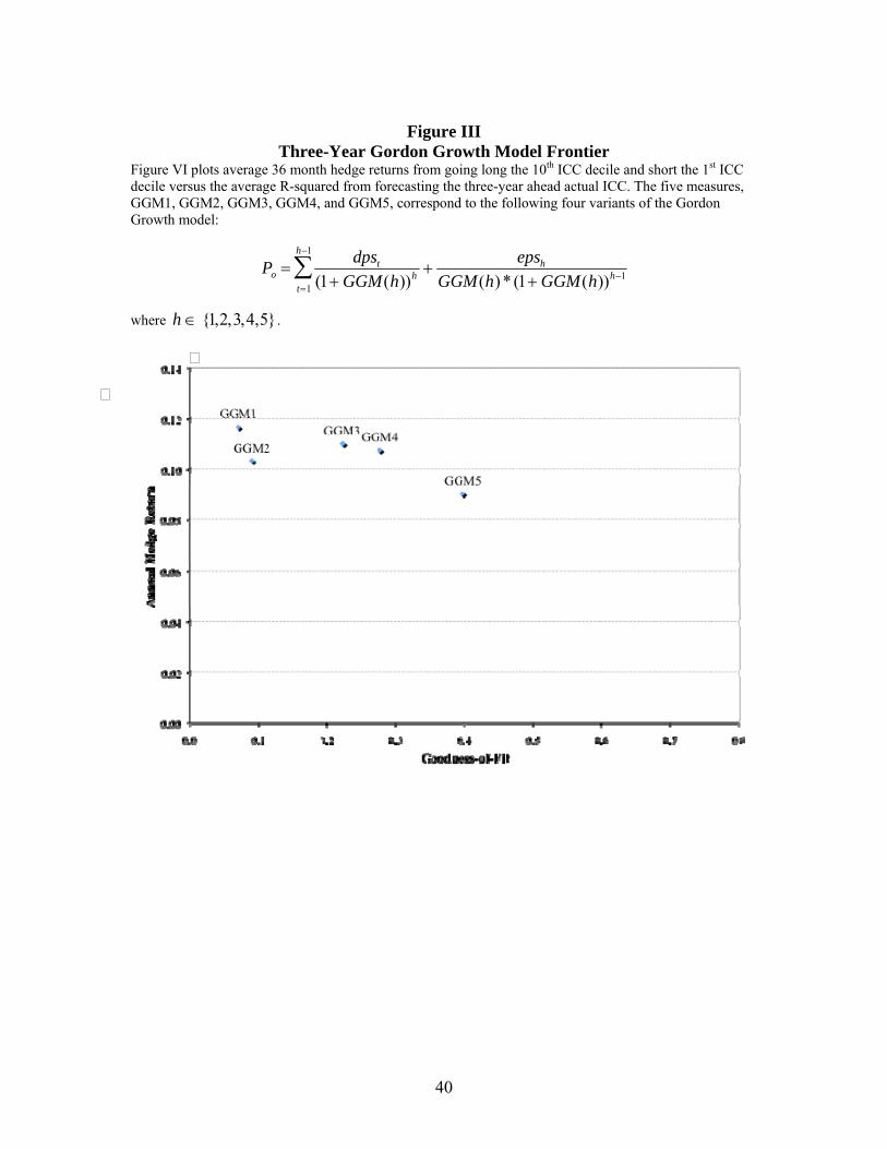
40

Figure III

Three-Year Gordon Growth Model Frontier Figure VI plots average 36 month hedge returns from going long the 10th ICC decile and short the 1st ICC decile versus the average R-squared from forecasting the three-year ahead actual ICC. The five measures, GGM1, GGM2, GGM3, GGM4, and GGM5, correspond to the following four variants of the Gordon Growth model:

Po dpst

(1 GGM(h))ht1

h1

epsh

GGM(h) * (1 GGM(h))h1

where

h {1,2,3,4,5}.