Option-implied information: What's the vol surface got to do ...
33
Review of Derivatives Research https://doi.org/10.1007/s11147-020-09166-0 Option-implied information: What’s the vol surface got to do with it? Maxim Ulrich 1 · Simon Walther 2 © The Author(s) 2020 Abstract We find that option-implied information such as forward-looking variance, skewness and the variance risk premium are sensitive to the way the volatility surface is con- structed. For some state-of-the-art volatility surfaces, the differences are economically surprisingly large and lead to systematic biases, especially for out-of-the-money put options. Estimates for risk-neutral variance differ across volatility surfaces by more than 10% on average, leading to variance risk premium estimates that differ by 60% on average. The variations are even larger for risk-neutral skewness. To overcome this problem, we propose a volatility surface that is built with a one-dimensional ker- nel regression. We assess its statistical accuracy relative to existing state-of-the-art parametric, semi- and non-parametric volatility surfaces by means of leave-one-out cross-validation, including the volatility surface of OptionMetrics. Based on 14 years of end-of-day and intraday S&P 500 and Euro Stoxx 50 option data we conclude that the proposed one-dimensional kernel regression represents option market information more accurately than existing approaches of the literature. Keywords Option-implied · Risk-neutral variance · Risk-neutral density · Tail risk · Option standardization · Interpolation JEL Classification G13 · G17 · C14 We are thankful for comments from Marliese Uhrig-Homburg, Jonathan Wright, Melanie Schienle and Philipp Schuster, seminar participants at the KIT and two anonymous referees. Special thanks to Thorsten Luedecke from the Karlsruhe Capital Market Database and to Deutsche Boerse for providing access to the Euro Stoxx 50 options. Simon Walther gratefully acknowledges financial support by the Konrad-Adenauer-Stiftung. B Simon Walther [email protected] Maxim Ulrich [email protected] 1 Karlsruhe Institute of Technology (KIT), Bluecherstr. 17, E008, 76185 Karlsruhe, Germany 2 Karlsruhe Institute of Technology (KIT), Bluecherstr. 17, E004, 76185 Karlsruhe, Germany 123
-
Upload
khangminh22 -
Category
Documents
-
view
0 -
download
0
Transcript of Option-implied information: What's the vol surface got to do ...
Review of Derivatives Researchhttps://doi.org/10.1007/s11147-020-09166-0
Option-implied information: What’s the vol surface got todo with it?
Maxim Ulrich1 · Simon Walther2
© The Author(s) 2020
AbstractWe find that option-implied information such as forward-looking variance, skewnessand the variance risk premium are sensitive to the way the volatility surface is con-structed. For some state-of-the-art volatility surfaces, the differences are economicallysurprisingly large and lead to systematic biases, especially for out-of-the-money putoptions. Estimates for risk-neutral variance differ across volatility surfaces by morethan 10% on average, leading to variance risk premium estimates that differ by 60%on average. The variations are even larger for risk-neutral skewness. To overcomethis problem, we propose a volatility surface that is built with a one-dimensional ker-nel regression. We assess its statistical accuracy relative to existing state-of-the-artparametric, semi- and non-parametric volatility surfaces by means of leave-one-outcross-validation, including the volatility surface of OptionMetrics. Based on 14 yearsof end-of-day and intraday S&P 500 and Euro Stoxx 50 option data we conclude thatthe proposed one-dimensional kernel regression represents option market informationmore accurately than existing approaches of the literature.
Keywords Option-implied · Risk-neutral variance · Risk-neutral density · Tail risk ·Option standardization · Interpolation
JEL Classification G13 · G17 · C14
We are thankful for comments from Marliese Uhrig-Homburg, Jonathan Wright, Melanie Schienle andPhilipp Schuster, seminar participants at the KIT and two anonymous referees. Special thanks to ThorstenLuedecke from the Karlsruhe Capital Market Database and to Deutsche Boerse for providing access to theEuro Stoxx 50 options. Simon Walther gratefully acknowledges financial support by theKonrad-Adenauer-Stiftung.
B Simon [email protected]
Maxim [email protected]
1 Karlsruhe Institute of Technology (KIT), Bluecherstr. 17, E008, 76185 Karlsruhe, Germany
2 Karlsruhe Institute of Technology (KIT), Bluecherstr. 17, E004, 76185 Karlsruhe, Germany
123
M. Ulrich, S. Walther
1 Introduction
Many popular option-implied metrics such as risk-neutral variance, skewness andthe variance risk premium are calculated based on an estimate of the option-impliedvolatility surface. We document in this paper that the method for constructing thevolatility surface affects these standard option-implied quantities. Our findings holdmore generally for any quantity that is extracted from the aggregation of option pricesalong the strike range.
State-of-the-art methodologies such as the semi-parametric spline interpolation1 ofFiglewski (2008) or the three-dimensional kernel regression of OptionMetrics (2016)produce surprisingly large differences in standard option-implied quantities. In oursample for S&P500 options (2004–2017), Bakshi et al. (2003) risk-neutral variance formedium-term maturities, computed with exactly the same procedure, but based on thevolatility surface from the interpolation scheme of Figlewski (2008) or OptionMetrics(2016), differs in relative terms by more than 10% on average. The 1-month-aheadvariance risk premium varies across both volatility surfaces by a relative margin ofon average 60%. Differences are even more troublesome for risk-neutral skewness,where we document relative differences in the order of 200% and more.
The key question to ask is which volatility surface represents market informationmost accurately? As information is extracted from option prices by means of deter-ministic manipulations of the observed portions of the volatility surface, it is naturalthat it is the most accurate volatility surface that also reprices options most accu-rately. We therefore perform a detailed empirical investigation to understand whichvolatility surface captures market information most accurately. Our test incorporatesthe semi-parametric spline interpolation (Figlewski 2008), a three-dimensional non-parametric kernel regression (OptionMetrics 2016), and the parametricGram–Charlierexpansion (Beber and Brandt 2006). In addition, we also propose an one-dimensionalnon-parametric kernel regression. We compare the statistical accuracy of these fourvolatility surfaces bymeans of leave-one-out cross-validation rootmean squared errors(RMSEs) andmean absolute errors (MAE). Calculating the average integrated squaredsecond derivative of the respective implied volatility smiles allows us to identify dif-ferences in smoothness. Our tests expand across two dimensions: (i) options on theS&P 500 and on the Euro Stoxx 50 and (ii) with an end-of-day and intraday frequency.The time span of the analysis is 2004–2017 for US data and 2002–2017 for Europeandata.
Our main findings are as follows: First, the one-dimensional kernel regressiongenerates the most accurate volatility surface for S&P 500 options by means of thelowest leave-one-out cross-validation RMSE and MAE. This holds for intraday andfor end-of-day data.
Second, for the end-of-day analysis of S&P 500 options, the spline-based volatilitysurface turns out to be the second best, with a RMSE (MAE) that is on average 128%(91%) higher than the RMSE of the one-dimensional kernel regression surface. The
1 The spline interpolation represents an implied volatility smile parametrically. However, there is no explicitparametric form of the risk-neutral density (RND), that the volatility smile implies. For this reason, weconsider this methodology, and more broadly the class of parametric implied volatility models that do notallow to pin down the RND parametrically, as semi-parametric.
123
Option-implied information: What’s the vol surface got to…
three-dimensional kernel regression produces a RMSE that is more than 5 times largerthan the RMSE of the one-dimensional kernel regression and an 11 times higherMAE. The Gram–Charlier volatility surface produces the largest RMSEs (MAEs),on average over 9 (23) times larger than the RMSE (MAE) of the best performingvolatility surface. The results for Euro Stoxx 50 options confirm our general findings,though the one-dimensional kernel regression and the spline interpolation appear toperform roughly at par here.
Third, state-of-the-art volatility surfaces turn out to be less accurate than theone-dimensional kernel regression volatility surface because these surfaces do notaccurately capturemarket information in the thinly traded tails of the volatility surface.The volatility surface based on spline interpolation shows weakness in capturing theleft tail of short-term options. The three-dimensional kernel regression shows severeshortcomings in capturing the left tail of short-, medium- and long-term options. Themethod of the Gram–Charlier expansion partially captures the at-the-money region ofthe volatility smiles well, but shows otherwise shortcomings in capturing the left andright tail of options across all maturities.
Fourth, for the intraday analysis we find that the most accurate volatility surfaceis again the one that is generated by the one-dimensional kernel regression, if data isvery scarce. However, the indication about the most accurate method depends on thenumber of trades that are used to construct the implied volatility surface and divergesbetween the error measures.While the one-dimensional kernel regression continues tolead in most set-ups with respect to the RMSE, the spline interpolation quickly showslowerMAEs than all other methods as the number of trades grows. This finding can berationalized by occasional over-fitting in the spline method, which occurs less oftenif more trades are available.
Our analysis concludes that option-implied information can differ substantiallyacross volatility surfaces. The three-dimensional kernel regression of OptionMetrics(2016) underpredicts option-implied tail risk at the end-of-day data frequency, whichtranslates into systematic biases in risk-neutral skewness and variance. The Gram–Charlier expansion is not flexible enough to closely track observed option prices. Theone-dimensional kernel regression appears to produce the most accurate volatilitysurface for the end-of-day use-case and if data is very scarce. Yet, using the splineinterpolation might be beneficial if an intermediate amount of implied volatility obser-vations is available. In that case, the over-fitting tendency in the spline interpolationis already dampened enough to produce the lowest MAEs, although the performancespread to the one-dimensional kernel regression is not large.
Our research study adds to the growing empirical finance literature that exploitsoption-implied information. By now, this literature is too vast to be reviewed here indetail. Hence, we cannot give credit to all studies and have to leave out importantcontributions. However, we discuss a selection of recent studies and focus on howthese have constructed the option-implied volatility surface.
A large and diverse amount of research studies work with the volatility surface ofOptionMetrics (2016): For example, Buss and Vilkov (2012) estimate option-impliedcorrelations and CAPM betas and find that higher option-implied betas go along withhigher average returns. Chang et al. (2012) predict a stock’s beta based on Bakshi et al.(2003) implied volatility and skewness estimates. Martin and Wagner (2019) extract
123
M. Ulrich, S. Walther
a measure for predicting the risk premium for each stock from its associated impliedvolatility surface. Christoffersen et al. (2017) propose a parametric option pricingmodel where illiquidity is a driver of the jump intensity of the underlying and canthus explain time variation in the implied volatility surface. Du and Kapadia (2012)compare the information content of the VIX and the Bakshi et al. (2003) impliedvariance measure and construct a tail risk index from its difference. Hofmann andUhrig-Homburg (2018) use the wedge between implied volatility observations andrespective OptionMetrics (2016) estimates to construct a limits of arbitrage measure.
Driessen et al. (2009) compare portfolios of single stock options with optionson the index and find evidence for a substantial option-implied correlation risk pre-mium. Bollerslev and Todorov (2011) introduce various risk measures for realized andexpected continuous risk and jump risk under the empirical and risk-neutral probabilitymeasure and find that a significant portion of the equity risk premium is compensa-tion for jump risk. The option-implied volatility surface in these innovative studies isconstructed based on end-of-day closing prices and based on a version of the splineinterpolation methodology that we use in this paper.
Martin (2017) shows that options contain information about the lower bound ofthe underlying’s expected return. Schneider and Trojani (2015) construct tradableoption-implied strategies for higher moments. These studies do not interpolate theoption-implied volatility surface, but work with observed option-implied volatilities.
Wright (2016) adopts the multi-dimensional kernel regression of Aït-Sahalia andLo (1998) to construct a monthly option-implied volatility surface of real interestrates. The author pools all end-of-day volatilities (roughly 25 per day and maturity)within 1month to stabilize the procedure and obtain a sufficiently smooth volatilitysurface. Swanson (2016) highlights that pooling prevents that study from working at ahigher frequency. Moreover, Swanson (2016) suggests to use the spline methodologyto construct daily option-implied volatility surfaces. As evidence in Bliss and Pani-girtzoglou (2002) suggests, that method works well for 10 or more option prices perday and maturity. In order to stay in a non-parametric framework while still obtain-ing smoothness, Jackwerth and Rubinstein (1996) and Jackwerth (2000) propose amethod that directly fits the volatility surface to observed data by minimizing thesquared fitting error while at the same time maximizing the smoothness of the surface.Our research study contributes to this discussion, as we formally compare the sta-tistical accuracy and smoothness of several state-of-the-art volatility surfaces acrossdifferent frequencies and different currency zones. For our tests, we select two ker-nel regression approaches as representatives for the non-parametric class of volatilitysurfaces. These methods do not explicitly optimize for smoothness, thus enabling usto perform a fair evaluation between methods, since neither the kernel regression ofOptionMetrics (2016) nor the splinemethod of Figlewski (2008) or theGram–Charlierexpansion features an explicit smoothness treatment. As we document, especially theone-dimensional kernel regression is still well capable of producing smooth volatilitysurfaces.
A large body of the literature studies parametric representations of the impliedvolatility surface. An early example is Schönbucher (1999), who assumes a diffusion
123

Option-implied information: What’s the vol surface got to…
process for the evolution of implied volatility.2 He derives restrictions on the parame-ters to ensure arbitrage-freeness and to prevent the potential model-implied emergenceof bubbles in implied volatility as the maturity decreases. The latter leads to a con-straint that can essentially serve as a model for the volatility smile at a given maturity.Based on a two-dimensional diffusion for the forward price of an asset and its volatil-ity, Hagan et al. (2002) derive a closed-form solution for a parametric volatility smilein their SABR model. The model is completely specified by four parameters, whichessentially describe the level, skew and curvedness of the volatility smile. However,as Gatheral (2006) points out, the lack of a mean reversion component in the volatilitydiffusionmakes it only applicable to short-maturity options. In his SVI model, Gatheral(2004) assumes a parametric function for the volatility smile that is similar to the rep-resentation of Schönbucher (1999), but features an additional parameter to locate thevolatility smile across the strike range. By construction, the SVI model assumes thatthe implied volatility smile becomes approximately linear in the tails. This assumptionis not always fulfilled in the data, which has triggered the development of generalizedversions of the SVI model that allow concavity, for example Zhao and Hodges (2013)or Damghani and Kos (2013). Damghani (2015) further elaborates on this work inthe context of the FX option market. His IVP model features an explicit treatmentof the bid-ask spreads in option prices and allows to incorporate liquiditiy factors.By adding a maturity interpolation scheme, he is able to capture the whole volatilitysurface with a dramatic reduction in parameters that need to be estimated. Figlewski(2008) follows a different approach: He argues to use a 4th-order smoothing splinewith one knot point at-the-money to model the volatility smile at each maturity sep-arately. The higher amount of free parameters is accepted to reach a higher accuracywhile still smoothing out noise. In our study, we use the method of Figlewski (2008)as representative of the class of parametric models of the implied volatility surface.
Survey and methodology papers that are closest to ours are Jackwerth (1999),Jondeau and Rockinger (2000), Bliss and Panigirtzoglou (2002) and Bahaludin andAbdullah (2017). Relative to these studies, our empirical assessment covers a muchlonger time span (14 years), US and EU equity option markets and distinguishesbetween characteristics of the input option data sets.
2 Data
We use data for two of the most actively traded equity option contracts: options on theS&P 500 and options on the Euro Stoxx 50. The former is traded at the CBOE whilethe latter is traded at the Eurex. The S&P 500 and the Euro Stoxx 50 do both standfor the Blue Chip stocks of their respective currency zone. Both option contracts areof European exercise style.
Historical data for S&P 500 options come from the CBOE Livevol data shop. Wecollect both end-of-day bid-ask prices as well as intraday transaction prices. For the
2 Assuming a diffusion process for implied volatility is different from a diffusion process for the volatilityof the underlying, as in Heston (1993). In themodel of Schönbucher (1999), movements in implied volatilityare correlated with movements in the underlying, though explicitly feature components that are independentof the underlying asset.
123

M. Ulrich, S. Walther
Table 1 Data summary
EOD Trades
S&P 500 Euro Stoxx 50 S&P 500 Euro Stoxx 50
Total number of price observations 9,246,926 6,877,495 43,749,042 16,921,911
Avg number of maturities per day 17.21 16.58 16.96 12.65
Avg number of strikes per maturity 61.27 45.28 16.97 5.93
Avg number of price observa-tions per day and maturity
157.58 104.22 740.43 356.84
Total number of short-term ATM prices 771,000 73,000 24,627,422 5,866,507
Total number of short-term left tail prices 1,326,413 274,227 4,449,056 1,956,662
Total number of short-term right tail prices 293,823 198,558 1,330,209 903,600
Total number of medium-term ATM prices 1,186,655 293,028 7,348,889 3,148,740
Total number of medium-term left tail prices 3,536,880 1,218,912 3,996,122 3,016,860
Total number of medium-term right tail prices 1,048,097 982,266 1,628,093 1,586,504
Total number of long-term ATM prices 120,389 340,796 100,016 168,532
Total number of long-term left tail prices 656,001 1,768,878 179,571 170,934
Total number of long-term right tail prices 307,668 1,727,830 89,664 103,572
This table provides some aggregated summary statistics of our option panel. ‘EOD’ stands for ‘end-of-day’(data-rich environment), whereas the ‘Trades’ columns summarize the aggregated data for our intradayanalysis (data-poor environment). Options with a remaining maturity of less than 30 days are consideredshort-term, options with 30-365 days to maturity are considered medium-term and longer maturity optionsare considered long-term. At-the-money (ATM) options have a moneyness between 0.95 and 1.05. Optionswith a moneyness below 0.95 are considered as ’left tail’ and options with a moneyness above 1.05 areconsidered as ’right tail’
end-of-day data set, we use the mid price for our calculations, whereas we use actualtrade prices for the intraday data set. The end-of-day data is from January 2004 toJuly 2017. The intraday data spans the period January 2004 to October 2017. The datacomes with the matched bid and ask prices of the underlying at the point of time ofthe record.
We obtain end-of-day settlement prices and intraday transaction prices for the EuroStoxx 50 options and the underlying Euro Stoxx 50 index from theKarlsruher Kapital-marktdatenbank (KKMDB), which is hosted at the Finance Institute of the KarlsruheInstitute of Technology. The KKMDB receives its data directly from the Eurex andStoxx. The index data comes in 15 second intervals, while the intraday option datais time stamped at the point of time of the trade. We match the option trade with theindex price directly at or prior to the trade’s time stamp. The end-of-day data spansJanuary 2002 to September 2017, whereas the intraday data covers the period January2003 to September 2017. Table 1 summarizes our option data sets in more detail.
For the risk-free rate, we use the US-Dollar and Euro OIS curves from Bloomberg,which come in discrete maturities between 1 day and 20 years and which we obtainat the daily frequency. We match each option record with the risk-free rate for itsrespective date. We interpolate the OIS rate linearly along the maturity dimension tomatch the maturity of the respective option.
We apply a number of filtering steps to ensure that only valid option prices enter thestandardization. We only consider options with a price that fulfills basic no-arbitrage
123
Option-implied information: What’s the vol surface got to…
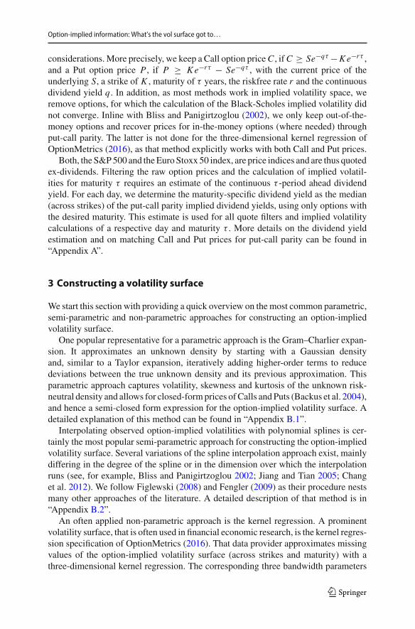
considerations.More precisely, we keep a Call option priceC , ifC ≥ Se−qτ −K e−rτ ,and a Put option price P , if P ≥ K e−rτ − Se−qτ , with the current price of theunderlying S, a strike of K , maturity of τ years, the riskfree rate r and the continuousdividend yield q. In addition, as most methods work in implied volatility space, weremove options, for which the calculation of the Black-Scholes implied volatility didnot converge. Inline with Bliss and Panigirtzoglou (2002), we only keep out-of-the-money options and recover prices for in-the-money options (where needed) throughput-call parity. The latter is not done for the three-dimensional kernel regression ofOptionMetrics (2016), as that method explicitly works with both Call and Put prices.
Both, the S&P500 and theEuroStoxx 50 index, are price indices and are thus quotedex-dividends. Filtering the raw option prices and the calculation of implied volatil-ities for maturity τ requires an estimate of the continuous τ -period ahead dividendyield. For each day, we determine the maturity-specific dividend yield as the median(across strikes) of the put-call parity implied dividend yields, using only options withthe desired maturity. This estimate is used for all quote filters and implied volatilitycalculations of a respective day and maturity τ . More details on the dividend yieldestimation and on matching Call and Put prices for put-call parity can be found in“Appendix A”.
3 Constructing a volatility surface
We start this section with providing a quick overview on themost common parametric,semi-parametric and non-parametric approaches for constructing an option-impliedvolatility surface.
One popular representative for a parametric approach is the Gram–Charlier expan-sion. It approximates an unknown density by starting with a Gaussian densityand, similar to a Taylor expansion, iteratively adding higher-order terms to reducedeviations between the true unknown density and its previous approximation. Thisparametric approach captures volatility, skewness and kurtosis of the unknown risk-neutral density and allows for closed-formprices ofCalls andPuts (Backus et al. 2004),and hence a semi-closed form expression for the option-implied volatility surface. Adetailed explanation of this method can be found in “Appendix B.1”.
Interpolating observed option-implied volatilities with polynomial splines is cer-tainly the most popular semi-parametric approach for constructing the option-impliedvolatility surface. Several variations of the spline interpolation approach exist, mainlydiffering in the degree of the spline or in the dimension over which the interpolationruns (see, for example, Bliss and Panigirtzoglou 2002; Jiang and Tian 2005; Changet al. 2012). We follow Figlewski (2008) and Fengler (2009) as their procedure nestsmany other approaches of the literature. A detailed description of that method is in“Appendix B.2”.
An often applied non-parametric approach is the kernel regression. A prominentvolatility surface, that is often used in financial economic research, is the kernel regres-sion specification of OptionMetrics (2016). That data provider approximates missingvalues of the option-implied volatility surface (across strikes and maturity) with athree-dimensional kernel regression. The corresponding three bandwidth parameters
123

M. Ulrich, S. Walther
are fixed in OptionMetrics (2016). To keep our paper self-contained, we provide in“Appendix B.3” a detailed description of that non-parametric approach.
We now continue to present our own kernel regression specification, that combinesadvantages of the above mentioned methods. First, it is a non-parametric approach,which ensures flexibility. Second, it is essentially only one-dimensional, which makesitmore robust and less data intensive than existingmulti-dimensional kernel regressionapproaches. Third, our approach ensures the volatility surface to be arbitrage-free,borrowing a technique from Fengler (2009). Fourth, conditional on having sufficientdata, our approach takes special care of capturing market information that is hiddenin the thinly traded tails.
3.1 One-dimensional kernel regression with tail extrapolation
We continue here to present in detail our suggested variation of the kernel regressionmethod that was popularized by Aït-Sahalia and Lo (1998). Aït-Sahalia and Lo (1998)propose to approximate unobserved option-implied volatilities by the following kernelregression set-up:
σ (Fj , K j , τ j ) =N∑
i=1
k(Fj − Fi ) k(K j − Ki ) k(τ j − τi )∑Ni=1 k(Fj − Fi ) k(K j − Ki ) k(τ j − τi )
× σ(Fi , Ki , τi ), (1)
where N is the number of observed option prices that enter the kernel regression asinputs, σ(.) is the observed Black-Scholes implied volatility and σ is the interpolatedBlack-Scholes implied volatility for a desired tuple of strike K j , forward price of theunderlying Fj and maturity τ j . The kernel function k(x) has a Gaussian shape withits own bandwidth parameter hx for each dimension, i.e.,
k(x) = 1√2π
e−
(x22hx
)
. (2)
We are now going to present refinements that distinguish our approach from the testedapplication in Aït-Sahalia and Lo (1998). First, we reduce the input dimension byone unit, as we combine the underlying forward price with the strike level. Moreprecisely, we define the observed moneyness measure as mi = Ki
Fiand apply the
kernel regression to m j − mi instead of Fj − Fi and K j − Ki .3 In most cases, thisstep can be regarded as a mere technical rescaling of the strike axis, which does notaffect the interpolation accuracy of the technique. In our end-of-day set-up, we onlyuse the price observations of a single day to construct the respective day’s impliedvolatility surface, which all have the same underlying price as they are observed atthe same point of time. Similarly, in the intraday set-ups, we construct the impliedvolatility surfaces based on subsequent option trade observations. In the vast majorityof cases, the change in the underlying price between two option trades is very small,
3 Although this adjustment has already been proposed by Aït-Sahalia and Lo (1998), their subsequentempirical analysis works with K and F , separately.
123
Option-implied information: What’s the vol surface got to…
such that the underlying forward price can be considered approximately constant forthe employed set of option trade observations.
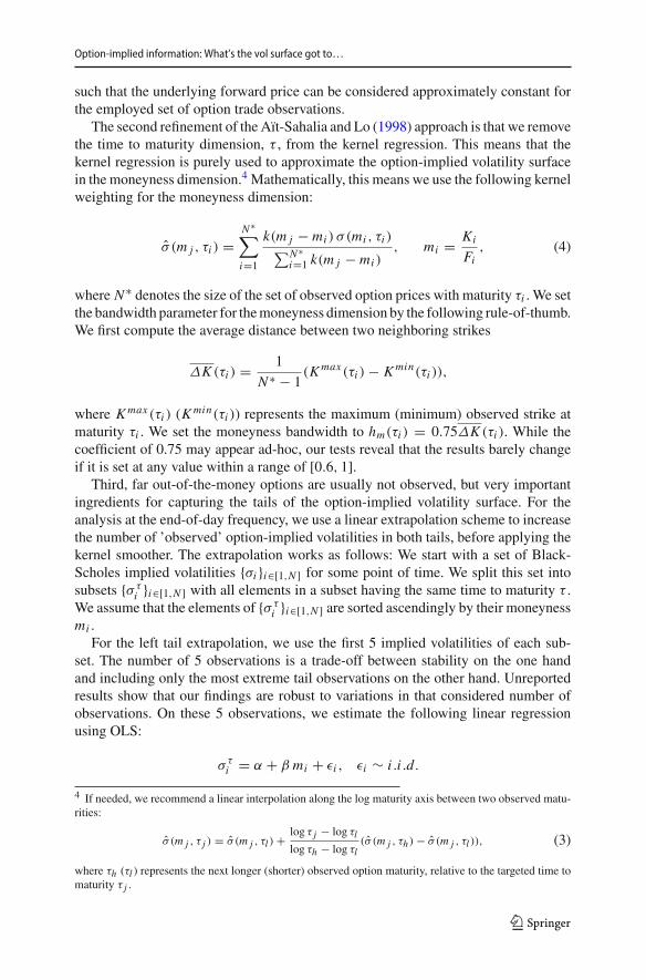
The second refinement of the Aït-Sahalia and Lo (1998) approach is that we removethe time to maturity dimension, τ , from the kernel regression. This means that thekernel regression is purely used to approximate the option-implied volatility surfacein the moneyness dimension.4 Mathematically, this means we use the following kernelweighting for the moneyness dimension:
σ (m j , τi ) =N∗∑
i=1
k(m j − mi ) σ (mi , τi )∑N∗i=1 k(m j − mi )
, mi = Ki
Fi, (4)
where N∗ denotes the size of the set of observed option prices with maturity τi . We setthe bandwidth parameter for themoneyness dimension by the following rule-of-thumb.We first compute the average distance between two neighboring strikes
ΔK (τi ) = 1
N∗ − 1(K max (τi ) − K min(τi )),
where K max (τi ) (K min(τi )) represents the maximum (minimum) observed strike atmaturity τi . We set the moneyness bandwidth to hm(τi ) = 0.75ΔK (τi ). While thecoefficient of 0.75 may appear ad-hoc, our tests reveal that the results barely changeif it is set at any value within a range of [0.6, 1].
Third, far out-of-the-money options are usually not observed, but very importantingredients for capturing the tails of the option-implied volatility surface. For theanalysis at the end-of-day frequency, we use a linear extrapolation scheme to increasethe number of ’observed’ option-implied volatilities in both tails, before applying thekernel smoother. The extrapolation works as follows: We start with a set of Black-Scholes implied volatilities {σi }i∈[1,N ] for some point of time. We split this set intosubsets {σ τ
i }i∈[1,N ] with all elements in a subset having the same time to maturity τ .We assume that the elements of {σ τ
i }i∈[1,N ] are sorted ascendingly by their moneynessmi .
For the left tail extrapolation, we use the first 5 implied volatilities of each sub-set. The number of 5 observations is a trade-off between stability on the one handand including only the most extreme tail observations on the other hand. Unreportedresults show that our findings are robust to variations in that considered number ofobservations. On these 5 observations, we estimate the following linear regressionusing OLS:
σ τi = α + β mi + εi , εi ∼ i .i .d.
4 If needed, we recommend a linear interpolation along the log maturity axis between two observed matu-rities:
σ (m j , τ j ) = σ (m j , τl ) + log τ j − log τl
log τh − log τl(σ (m j , τh) − σ (m j , τl )), (3)
where τh (τl ) represents the next longer (shorter) observed option maturity, relative to the targeted time tomaturity τ j .
123

M. Ulrich, S. Walther
Fig. 1 Effect of tail extrapolation on kernel regression. This figure visualizes for a particular day of thesample, May 22nd, 2012, the effect of the linear tail extrapolation on the option-implied volatility smilefor Euro Stoxx 50 options with 24 days to maturity. The left panel shows the kernel regression without tailextrapolation, the right panel includes the tail extrapolation. The dots mark observed (and artificial) impliedvolatility observations, the line depicts the interpolation
Table 2 Cross-validation errors for refinement steps of the kernel regression
Step S&P 500 Euro Stoxx 50
RMSE MAE RMSE MAE
Initial 0.0479 0.0139 0.1964 0.0518
No maturity dimension 0.0109 0.0023 0.0156 0.0024
Tail extrapolation 0.0091 0.0019 0.0101 0.0021
No-arbitrage enforcement 0.0092 0.0019 0.100 0.0019
This table shows the leave-one-out cross-validation root mean squared error (RMSE) and mean absoluteerror (MAE) for our refinements steps of the kernel regression method of Aït-Sahalia and Lo (1998).All numbers refer to end-of-day data. Initial represents the original method, applied day by day. We firstremove the maturity dimension (No maturity dimension) and then add the linear tail extrapolation in impliedvolatility space (Tail extrapolation). Finally, we additionally enforce no-arbitrage on the volatility surfacein the No-arbitrage enforcement step
Starting from the lowest observed moneyness, we proceed in steps of ΔK (τi ) andcalculate the extrapolated implied volatility as σ (m) = α + β m until reaching amoneyness of m = 0.4. We proceed similarly for the right tail, using the last 5observations in {σ τ
i }i∈[1,N ] and extrapolating from the largest observed moneynessin steps of ΔK (τi ) until a final moneyness of 1.6. We use the union of observedimplied volatilities and thus artificially created implied volatilities as inputs for thekernel regression. Figure 1 presents the tail extrapolation visually for a sample dayand maturity.
The last refinement that we apply to the Aït-Sahalia and Lo (1998) methodology isto guarantee that the resulting option-implied volatility surface is consistent with anarbitrage-free asset market by applying the algorithm of Fengler (2009).
Table 2 displays the performance gains that we achieve with each adjustment of theAït-Sahalia and Lo (1998) method. Clearly, dropping the maturity dimension from the
123
Option-implied information: What’s the vol surface got to…
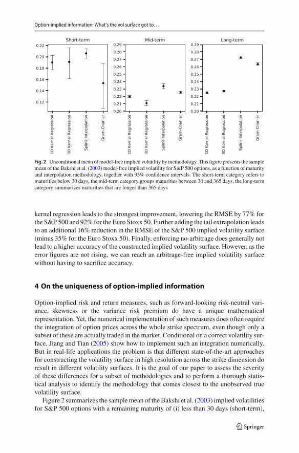
Fig. 2 Unconditionalmean ofmodel-free implied volatility bymethodology. This figure presents the samplemean of the Bakshi et al. (2003) model-free implied volatility for S&P 500 options, as a function of maturityand interpolation methodology, together with 95% confidence intervals. The short-term category refers tomaturities below 30 days, the mid-term category groups maturities between 30 and 365 days, the long-termcategory summarizes maturities that are longer than 365 days
kernel regression leads to the strongest improvement, lowering the RMSE by 77% forthe S&P 500 and 92% for the Euro Stoxx 50. Further adding the tail extrapolation leadsto an additional 16% reduction in the RMSE of the S&P 500 implied volatility surface(minus 35% for the Euro Stoxx 50). Finally, enforcing no-arbitrage does generally notlead to a higher accuracy of the constructed implied volatility surface. However, as theerror figures are not rising, we can reach an arbitrage-free implied volatility surfacewithout having to sacrifice accuracy.
4 On the uniqueness of option-implied information
Option-implied risk and return measures, such as forward-looking risk-neutral vari-ance, skewness or the variance risk premium do have a unique mathematicalrepresentation. Yet, the numerical implementation of suchmeasures does often requirethe integration of option prices across the whole strike spectrum, even though only asubset of these are actually traded in themarket. Conditional on a correct volatility sur-face, Jiang and Tian (2005) show how to implement such an integration numerically.But in real-life applications the problem is that different state-of-the-art approachesfor constructing the volatility surface in high resolution across the strike dimension doresult in different volatility surfaces. It is the goal of our paper to assess the severityof these differences for a subset of methodologies and to perform a thorough statis-tical analysis to identify the methodology that comes closest to the unobserved truevolatility surface.
Figure 2 summarizes the samplemean of the Bakshi et al. (2003) implied volatilitiesfor S&P 500 options with a remaining maturity of (i) less than 30 days (short-term),
123
M. Ulrich, S. Walther
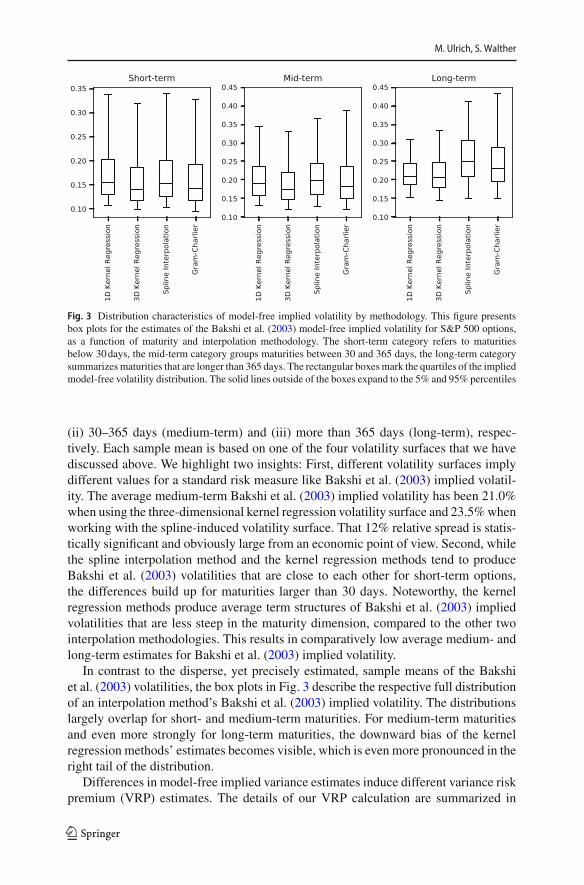
Fig. 3 Distribution characteristics of model-free implied volatility by methodology. This figure presentsbox plots for the estimates of the Bakshi et al. (2003) model-free implied volatility for S&P 500 options,as a function of maturity and interpolation methodology. The short-term category refers to maturitiesbelow 30days, the mid-term category groups maturities between 30 and 365 days, the long-term categorysummarizesmaturities that are longer than 365 days. The rectangular boxesmark the quartiles of the impliedmodel-free volatility distribution. The solid lines outside of the boxes expand to the 5% and 95% percentiles
(ii) 30–365 days (medium-term) and (iii) more than 365 days (long-term), respec-tively. Each sample mean is based on one of the four volatility surfaces that we havediscussed above. We highlight two insights: First, different volatility surfaces implydifferent values for a standard risk measure like Bakshi et al. (2003) implied volatil-ity. The average medium-term Bakshi et al. (2003) implied volatility has been 21.0%when using the three-dimensional kernel regression volatility surface and 23.5%whenworking with the spline-induced volatility surface. That 12% relative spread is statis-tically significant and obviously large from an economic point of view. Second, whilethe spline interpolation method and the kernel regression methods tend to produceBakshi et al. (2003) volatilities that are close to each other for short-term options,the differences build up for maturities larger than 30 days. Noteworthy, the kernelregression methods produce average term structures of Bakshi et al. (2003) impliedvolatilities that are less steep in the maturity dimension, compared to the other twointerpolation methodologies. This results in comparatively low average medium- andlong-term estimates for Bakshi et al. (2003) implied volatility.
In contrast to the disperse, yet precisely estimated, sample means of the Bakshiet al. (2003) volatilities, the box plots in Fig. 3 describe the respective full distributionof an interpolation method’s Bakshi et al. (2003) implied volatility. The distributionslargely overlap for short- and medium-term maturities. For medium-term maturitiesand even more strongly for long-term maturities, the downward bias of the kernelregression methods’ estimates becomes visible, which is even more pronounced in theright tail of the distribution.
Differences in model-free implied variance estimates induce different variance riskpremium (VRP) estimates. The details of our VRP calculation are summarized in
123

Option-implied information: What’s the vol surface got to…
Table 3 Average annualized monthly variance risk premium and Sharpe ratio
S&P 500 Euro Stoxx 50
Average VRP Sharpe ratio Average VRP Sharpe ratio
3D kernel regression 0.015 (0.0006) 0.44 0.019 (0.0006) 0.5
1D kernel regression 0.020 (0.0006) 0.54 0.029 (0.0007) 0.68
Spline interpolation 0.024 (0.0008) 0.57 0.028 (0.0007) 0.65
Gram–Charlier expansion 0.016 (0.0010) 0.26 0.024 (0.0007) 0.56
This table shows average annualized 1-month variance risk premia and VRP Sharpe Ratios. Standard errorsare given in parenthesis. The integration scheme and model for the physical variance expectations are thesame for all estimates, such that the only difference is the method for constructing the implied volatilitysurface
“Appendix C”. Table 3 summarizes the average annualizedVRP for S&P 500 and EuroStoxx 50 options for different volatility surfaces, respectively. The average annualizedVRP for S&P 500 (Euro Stoxx 50) options has been estimated to be between 1.5and 2.4% (1.9% and 2.9%), depending on the volatility surface. In relative terms,the spline-based volatility surface results on average in a 60% higher S&P 500 VRPestimate relative to the same estimate for the three-dimensional kernel regression. Thedifferences between the average VRP estimates are for nearly all pairs of methodsstatistically strongly significant. Monthly Sharpe ratios for the VRP range from 0.26to 0.57 for the S&P 500 and from 0.5 to 0.68 for the Euro Stoxx 50. We highlight thatthese economically large differences are a direct result of the choice of the inter- andextrapolation method that builds the basis for a volatility surface; the input data andthe integration scheme is the same across all methods.
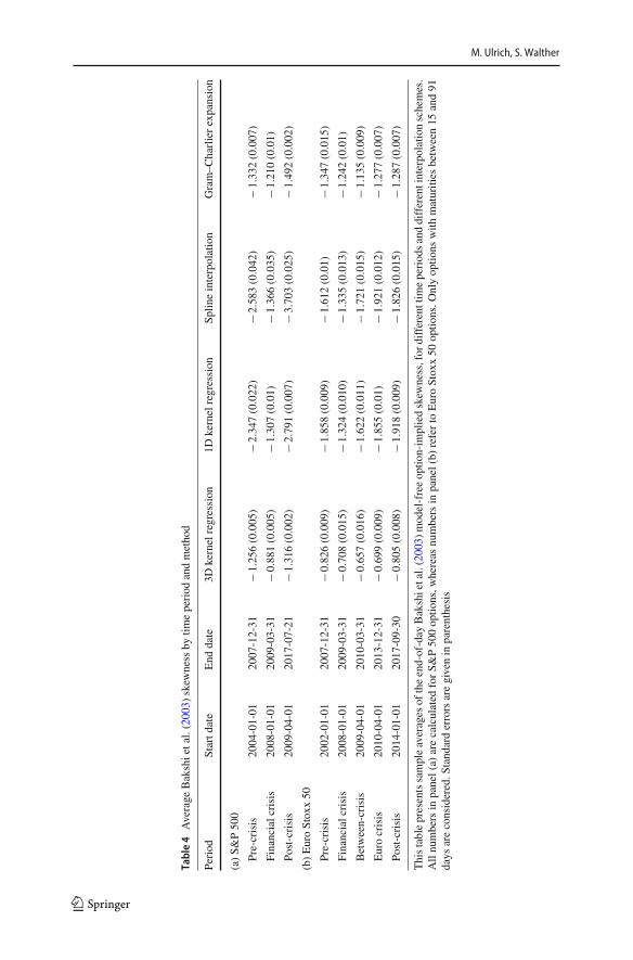
Table 4 states the sample mean of model-free option-implied skewness for matu-rities between 15 and 91 days. Option-implied skewness is calculated as in Bakshiet al. (2003) and reported for different sub-samples.5 We split the US data set intoa pre-financial-crisis, a crisis and a post-financial-crisis period. We apply the samecuts for the European data set, but further split the post-financial-crisis period into abetween-crisis-, an euro-crisis-, and a post-euro-crisis period due to the high impactof the European sovereign debt crisis for European stock markets. The risk-neutralskewness estimates are nearly all significantly different across different volatility sur-faces. The estimates with the three-dimensional kernel regression are roughly onlyhalf the size when compared to our proposed one-dimensional kernel regression orthe spline method. Further, the changes in the average risk-neutral skewness betweenone sub-period and the next also differ among the volatility surfaces, sometimes evendisagreeing on the sign of the change. For example, risk-neutral skewness estimatesbased on a spline interpolation get less negative on average after the Euro Crisis inEurope, while the estimates based on all other volatility surfaces get more negative.
In summary, information extracted from option markets is supposed to be unique.But our analysis has documented that this information is sensitive with regard to thevolatility surface that a researcher uses. We have shown that risk-neutral model-freeestimates for variance and skewness differ by a large margin across different state-of-
5 The results do not change qualitatively for different maturity intervals.
123
M. Ulrich, S. Walther
Table4
Average
Bakshietal.(200
3)skew
ness
bytim
eperiod
andmetho
d
Period
Startd
ate
End
date
3Dkernelregression
1Dkernelregression
Splin
einterpolation
Gram–C
harlierexpansion
(a)S&
P50
0
Pre-crisis
2004
-01-01
2007
-12-31
−1.256
(0.005
)−2
.347
(0.022
)−2
.583
(0.042
)−1
.332
(0.007
)
Financialcrisis
2008
-01-01
2009
-03-31
−0.881
(0.005
)−1
.307
(0.01)
−1.366
(0.035
)−1
.210
(0.01)
Post-crisis
2009
-04-01
2017
-07-21
−1.316
(0.002
)−2
.791
(0.007
)−3
.703
(0.025
)−1
.492
(0.002
)
(b)EuroStox
x50
Pre-crisis
2002
-01-01
2007
-12-31
−0.826
(0.009
)−1
.858
(0.009
)−1
.612
(0.01)
−1.347
(0.015
)
Financialcrisis
2008
-01-01
2009
-03-31
−0.708
(0.015
)−1
.324
(0.010
)−1
.335
(0.013
)−1
.242
(0.01)
Between-crisis
2009
-04-01
2010
-03-31
−0.657
(0.016
)−1
.622
(0.011
)−1
.721
(0.015
)−1
.135
(0.009
)
Eurocrisis
2010
-04-01
2013
-12-31
−0.699
(0.009
)−1
.855
(0.01)
−1.921
(0.012
)−1
.277
(0.007
)
Post-crisis
2014
-01-01
2017
-09-30
−0.805
(0.008
)−1
.918
(0.009
)−1
.826
(0.015
)−1
.287
(0.007
)
Thistablepresentssampleaverages
oftheend-of-day
Bakshietal.(200
3)model-freeoptio
n-im
pliedskew
ness,for
differenttim
eperiodsanddifferentinterpolatio
nschemes.
Allnu
mbersin
panel(a)
arecalculated
forS&
P50
0op
tions,w
hereas
numbersin
panel(b)
referto
EuroStox
x50
optio
ns.O
nlyop
tions
with
maturities
between15
and91
days
areconsidered.S
tand
arderrorsaregivenin
parenthesis
123

Option-implied information: What’s the vol surface got to…
the-art methods.While we have used the Bakshi et al. (2003) moments for explanatorypurpose, our findings hold more generally for any quantity that is extracted from theaggregation of option prices along the strike range.
5 Assessing the accuracy of a volatility surface
Here, we assess the relative advantages and disadvantages of different state-of-the-art volatility surfaces. Our previous findings have documented that standard option-implied measures differ across volatility surfaces. As these measures are deterministicfunctions of the volatility surface, it is natural that the most accurate volatility surfacedoes imply the most accurate option-implied risk measures.
At the same time, accuracy is only one of multiple practical considerations whenconstructing an implied volatility surface. It is, for example, well thinkable to accept alower accuracy in favor of a more informative representation of the volatility surface.Especially parametric models can provide such representations. Depending on themodel, single parameters can be interpreted directly and serve asmeasures that expressthe situation at the option market in lower dimension. For example, the parameters ofthe SVImodel of Gatheral (2004) inform about the level of the implied volatility smile,its rotation and how wide it is. Parametrization also allows to easily share an impliedvolatility surface, as it can be fully reconstructed from the relatively few parameters.The model for the volatility smile allows to extrapolate beyond observed option pricesin a manner that is consistent with the central part of the modeled volatility smile. No-arbitrage constraints can be incorporated into the construction of the implied volatilitysurface at the parameter estimation phase already (Damghani andKos 2013;Damghani2015). These arguments speak in favor of a parametric representation of the impliedvolatility surface. However in this study, we explore how accurate different volatilitysurfaces capture option market information. The result of our analysis can then serveas an important input, next to the previously mentioned concerns, for the choice of aconstruction method in practice.
One might also be willing to deliberately sacrifice some accuracy in the represen-tation of the observed implied volatilities in favor of a smoother volatility surface(Jackwerth 2000; Jackwerth and Rubinstein 1996). This is especially true, if the noisein the observations is expected to be large enough to not be fully canceled out by theinterpolation and smoothing method. In that case, the constructed volatility surfacewould show spikes or bumps, that would decrease its smoothness. On the other hand,a very smooth volatility surface might plane out important features of the observationsand thus introduce biases.6 Therefore, we are going to implement a thorough investi-gation on the statistical accuracy of popular volatility surfaces and compare them withrespect to their smoothness.
We follow a rich machine learning literature that assesses the accuracy of a modelbased on leave-one-out cross-validation (Geisser 1993; Kohavi 1995). The advantageof this cross-validation approach for our study is that every method that we use to
6 The introduction of biases by very smooth volatility surfaces can easily be seen by the fact that thesmoothest volatility surface is an uncurved plane.
123
M. Ulrich, S. Walther
construct an option-implied volatility surface is evaluated with data that was not usedto construct the surface. This allows us to detect over- and under-fitting.
We evaluate the statistical quality of each volatility surface with end-of-day andintraday data for S&P 500 and Euro Stoxx 50 options. End-of-day data is characterizedby a rich panel of option prices for different strikes and maturities, that all refer to thesame point of time. We call this to be the data-rich environment. In contrast, intradaydata is characterized by a limited amount of observed trade prices in a given timeinterval. We therefore call the intraday application to be a data-poor environment.The intraday set-up becomes increasingly data-poor as the considered time intervalfor pooling trade observations shrinks and thus the time resolution increases.7
The highest possible time resolution of a method is bound by the minimum amountof option trades that a method requires for constructing the option-implied volatilitysurface. Technically, the Gram–Charlier expansion requires only 3 observed optionprices for distinct strikes at the same maturity. Price observations at 3 different strikesare also the theoretical minimum for capturing the key characteristics level, slopeand curvature of the implied volatility smile. We undertake four independent intradayanalyses, namely relying on 3, 4, 5 and 10 observations per maturity.
For the end-of-day data set, the cross-validation works as follows: Given priceobservations of a day, we in turn leave out a single observation and calculate themethodology-implied estimate for that observation. We repeat this procedure for eachobserved option price. The data-poor set-up with 3, 4, 5 and 10 price observations permaturity is treated similarly: For each new transaction price, we use the corresponding3, 4, 5 or 10 preceding transaction prices with differing strike prices for the samematurity in order to create an estimate for the next transaction price. This approach isbasically assessing out-of-sample how well a volatility surface predicts future optionprices.
Given a set of N evaluation samples with Black-Scholes implied volatility obser-vations σ BS
i , i ∈ {1, ..., N }, our primary evaluation measure is the root mean squarederror (RMSE), that arises when comparing the respective method’s Black-Scholes-implied volatility estimator σ BS
i with the left out observation σ BSi :
RM SE =√√√√ 1
N
N∑
i=1
(σ BSi − σ BS
i )2. (5)
A detailed discussion of the relationship between the (root) mean squared error asevaluation criterion and the desire to obtain a smooth volatility surface can be foundin “Appendix D”. By squaring the errors, the RMSE penalizes large deviations ofthe constructed volatility surface from the observed implied volatilities more stronglythan small deviations. However, as discussed above, one might be willing to acceptoccasional large errors in favor of a smoother volatility surface. This is especially true,if one expects such large errors to be due to outliers, that are not representative of the
7 End-of-day data does not necessarily create a data-rich environment. For some options, only a handfulof strikes are traded, thus effectively constituting a data-poor environment in end-of-day data. On the otherhand, if the time interval for pooling intraday trade prices becomes large enough, there will likely be enoughobservations for distinct strikes to constitute a data-rich environment.
123
Option-implied information: What’s the vol surface got to…
true unobserved volatility surface. For this reason, we also calculate the mean absoluteerror (MAE),
M AE = 1
N
N∑
i=1
∣∣∣σ BSi − σ BS
i
∣∣∣ , (6)
which is less responsive to such occasional large errors and is still comparably low, ifthese errors only occur seldom and the remaining fit is good. For both error measures,we exclude observations with an implied volatility above 10.8
We also compare the end-of-day volatility surfaces with respect to their smoothnessdirectly. Following Jackwerth (2000), we measure smoothness as the sum of squaredsecond derivatives of the implied volatility surface along the moneyness dimension.More precisely, for each day t and maturity τ , we consider a moneyness range of[1−k s
√τ , 1+k s
√τ ], where s is an estimate for the unconditional annual volatility
of the underlying and k is a fixmultiple.We discretize this range in steps ofΔ = 2ks√
τ
99and construct the volatility smile {σ BS
j,t,τ } j∈[0,100] for the grid points of that day andmaturity with each method. Our measure for the smoothness of the smile is thencalculated as
St,τ =99∑
j=1
(σ BS
j−1,t,τ − 2σ BSj,t,τ + σ BS
j+1,t,τ
Δ2
). (7)
Finally, we compute the mean of that smoothness measure across all days andmaturities and take the square root for better readability. In that, we exclude the 1% ofthe smiles with the highest and the 1%with the lowest smoothness measure to mitigatethe impact of the tails of the distribution of smoothness figures on the mean estimates.
6 Findings
This section summarizes key findings of our empirical assessment of the statisticalquality of different state-of-the-art volatility surfaces. We start with the end-of-dayanalysis for S&P 500 and Euro Stoxx 50 options. This section ends with the findingsfor the intraday analysis.
6.1 End-of-day: data-rich environment
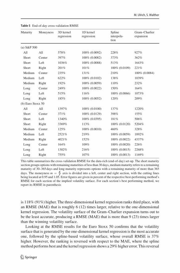
The aggregated RMSEs for the end-of-day, data-rich, environment are summarizedin Table 5, the respective MAE error figures can be found in Table 9 in “AppendixE”. For S&P 500 options we find that the volatility surface from the one-dimensionalkernel regression produces the lowest RMSE (0.0092) and MAE (0.0019). The splineinterpolation inducedvolatility surface ranks secondwith anoverallRMSE (MAE) that
8 In rare cases, observed option prices translate into unreasonably high implied volatilities. Our thresholdof 10 leads to the exclusion of 0.012% or less of the data points, depending on the data set.
123
M. Ulrich, S. Walther
Table 5 End-of-day cross-validation RMSE
Maturity Moneyness 3D kernelregression
1D kernelregression
Splineinterpola-tion
Gram–Charlierexpansion
(a) S&P 500
All All 578% 100% (0.0092) 228% 927%
Short Center 397% 100% (0.0082) 373% 362%
Short Left 1036% 100% (0.0088) 513% 1643%
Short Right 201% 101% 100% (0.0109) 221%
Medium Center 235% 131% 210% 100% (0.0084)
Medium Left 622% 100% (0.0102) 138% 1039%
Medium Right 192% 100% (0.0059) 110% 232%
Long Center 249% 100% (0.0022) 150% 164%
Long Left 515% 116% 100% (0.0066) 1073%
Long Right 185% 100% (0.0052) 120% 209%
(b) Euro Stoxx 50
All All 1397% 100% (0.0100) 137% 1220%
Short Center 371% 100% (0.0129) 398% 155%
Short Left 1340% 100% (0.0395) 181% 506%
Short Right 3369% 113% 100% (0.0120) 5204%
Medium Center 125% 100% (0.0010) 460% 328%
Medium Left 2521% 219% 100% (0.0059) 1892%
Medium Right 4021% 152% 100% (0.0022) 4337%
Long Center 164% 109% 100% (0.0020) 226%
Long Left 1302% 216% 100% (0.0015) 2268%
Long Right 755% 107% 100% (0.0013) 1169%
This table summarizes the cross-validation RMSE for the data-rich (end-of-day) set-up. The short maturitysection groups optionswith remainingmaturities of less than 30 days,mediummaturity refers to a remainingmaturity of 30–365days and long maturity represents options with a remaining maturity of more than 365days. The moneyness m = K
F axis is divided into a left, center and right section, with the cutting linesbeing located at 0.95 and 1.05. Error figures are given in percent of the respective best-performing method’sRMSE for each section of the implied volatility surface. For each section’s best performing method, wereport its RMSE in parenthesis
is 118% (91%) higher. The three-dimensional kernel regression ranks third place, withan RMSE (MAE) that is roughly 6 (12) times larger, relative to the one-dimensionalkernel regression. The volatility surface of the Gram–Charlier expansion turns out tobe the least accurate, producing a RMSE (MAE) that is more than 9 (23) times largerthan the winning volatility surface.
Looking at the RMSE results for the Euro Stoxx 50 confirms that the volatilitysurface that is generated by the one-dimensional kernel regression is the most accurateone, followed by the spline-based volatility surface, whose overall RMSE is 37%higher. However, the ranking is reversed with respect to the MAE, where the splinemethod performs best and the kernel regression shows a 29%higher error. This reversal
123

Option-implied information: What’s the vol surface got to…
Table 6 Smoothness of thevolatility surface by method
Method S&P 500 Euro Stoxx 50
3D kernel regression 1657 (115) 3315 (213)
1D kernel regression 600 (55) 303 (24)
Spline interpolation 1402 (407) 196 (46)
Gram–Charlier expansion 623 (46) 1096 (73)
This table shows the average smoothness of the constructed impliedvolatility surface for each method. For each day and maturity, wesum up the squared second derivative along the moneyness dimen-sion, aggregate across all days and maturities by taking the mean andreport the root of this figure. The second derivative is calculated for amoneyness interval between− 3 and 3 times the unconditional volatil-ity of the underlying, de-annualized to the respective maturity. Dueto the existence of rare outliers, we remove the 1% largest and small-est single smoothness values from the calculation. Standard errors aregiven in parenthesis
is the result of a downward bias of the one-dimensional kernel regression in deep out-of-the-moneymedium-term optionswith amoneyness below 0.5. If these optionswereto be excluded from the error calculation, the one-dimensional kernel regression andthe spline method would produce basically the same MAE for Euro Stoxx 50 data.Finally, the three-dimensional kernel regression and the Gram–Charlier expansionproduce RMSEs (MAEs) that are 14 (25) and 12 (24) times higher, respectively.
We now continue to report the RMSE for different regions of the option-impliedvolatility surface. We split the option-implied volatility surface along the maturityand moneyness dimension. Options with a maturity of less than 30 calendar days areconsidered short-term, options with a maturity between 30 and 365 calendar days areconsidered medium-term, while options with a maturity of more than 1 year are calledlong-term. Along the moneyness axis, we label a moneyness of 0.95 to 1.05 as at-the-money (ATM), whereas the ‘left tail’ (‘right tail’) is characterized by a moneyness ofbelow (above) 0.95 (1.05). In combination, these splits yield nine different regions ofthe option-implied volatility surface, for which we calculate the RMSE and MAE ofeach method.
Looking at panels (a) and (b) of Tables 5 and 9 highlights that across all volatilitysurfaces, short-term options and left tail options produce the highest errors. For theS&P 500, the one-dimensional kernel regression performs best in most sections of theimplied volatility surface with respect to the RMSE and in all sections with respectto the MAE. Spline interpolation tends to outperform the one-dimensional kernelregression for medium- and long-term options for the Euro Stoxx 50, though, which ismore pronounced in the RMSE results than in theMAE results. The three-dimensionalkernel regression and the Gram-Charlier expansion do both show severe difficulties incapturing the left and the right tail of the surface. The problem of the Gram–Charliervolatility surface is that the parametric risk-neutral density approximation turns outto be insufficient for capturing market information in the tails. We identify that therelative weakness of the three-dimensional kernel regression is that it only considersoptions with a delta of 0.2–0.8, which ignores market information about the tails.
123

M. Ulrich, S. Walther
Weproceed by comparing the smoothness of the volatility surfaces. Table 6 displaysour smoothness measures, as defined in Eq. 7. A smooth volatility surface has lowsecond derivatives and thus a low smoothnessmeasure. Conversely, a high smoothnessmeasure is an indicator for a more curved volatility surface. The volatility surfaceof the three-dimensional kernel regression is the least smooth in our tests. On theother end, the one-dimensional kernel regression appears to be smoother than most ofthe alternatives. For the spline interpolation, there is an interesting divergence in thesmoothness measure between its comparably rough S&P 500 volatility surface and itsvery smooth Euro Stoxx 50 surface. This goes hand in hand with the low errors of thespline interpolation in constructing the Euro Stoxx 50 surface. It seems like the splineinterpolation is not able to cancel out all noise in the S&P 500 data, which producesa more curved volatility surface and higher fitting errors. At the same time, a smoothvolatility surface does not necessarily imply low errors, as can be seen from the S&P500 results for the Gram–Charlier expansion. That method might produce a smoothvolatility surface, though it does not accurately reflect the information in observedoption prices.
In short summary, the cross-validation of the data-rich environment recommendsto use a volatility surface that was constructed based on the one-dimensional kernelregression. The spline interpolation is a good alternative for Euro Stoxx 50 data, thoughappears to not be able to cancel out all noise in the S&P 500 data. The volatilitysurface of the Gram–Charlier expansion should only be applied if one is interestedin option-implied information from the at-the-money region and should be avoidedwhen inferring conclusions about the tails. The three-dimensional kernel regressionproduces RMSEs that, relative to the one-dimensional kernel regression, are roughly6 times larger for S&P 500 options and roughly 14 times larger for Euro Stoxx 50options.
6.2 Intraday: data-poor environment
Here, we summarize key findings for the intraday analysis. We start with the highesttime resolution (3 trades), followed by interpolations based on 4, 5 and 10 trades fordistinct strikes.
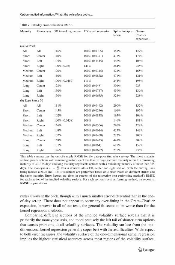
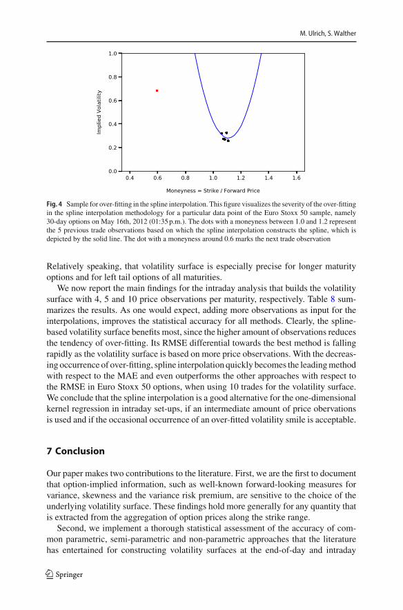
The findings from Table 7 (see Table 10 in “Appendix E” for MAE results) high-light that the one-dimensional kernel regression produces the most accurate overallvolatility surface. The three-dimensional kernel regression is the secondmost accuratesurface, though the performance differential is not as large as for the end-of-day set-up.In our sample, we find that the spline-based volatility surface suffers from frequentoutliers, which increases the RMSE enormously. This is not surprising, because thespline interpolation is prone to over-fitting when it is applied to very few observations.Figure 4 visualizes the potential problem of over-fitting when constructing the spline-based volatility surface with 5 or less data points. As the MAE is less responsive tooccasional large errors, which are a result of over-fitting, the spline interpolation per-forms better with respect to the MAE than with respect to the RMSE. It even shows aslightly lower MAE than the one-dimensional kernel regression for the Euro Stoxx 50intraday set-up with 3 trades. The volatility surface of the Gram–Charlier expansion
123
Option-implied information: What’s the vol surface got to…
Table 7 Intraday cross-validation RMSE
Maturity Moneyness 3D kernel regression 1D kernel regression Spline interpo-lation
Gram–Charlierexpansion)
(a) S&P 500
All All 116% 100% (0.0705) 381% 127%
Short Center 140% 100% (0.0371) 437% 174%
Short Left 105% 100% (0.1445) 346% 106%
Short Right 100% (0.05) 141% 264% 245%
Medium Center 120% 100% (0.0315) 421% 165%
Medium Left 110% 100% (0.0878) 471% 121%
Medium Right 100% (0.0459) 111% 244% 195%
Long Center 128% 100% (0.046) 301% 225
Long Left 130% 100% (0.0747) 459% 139%
Long Right 130% 100% (0.0635) 324% 228%
(b) Euro Stoxx 50
All All 111% 100% (0.0492) 290% 152%
Short Center 145% 100% (0.0246) 166% 192%
Short Left 102% 100% (0.0838) 195% 109%
Short Right 100% (0.0438) 109% 146% 181%
Medium Center 126% 100% (0.0306) 296% 228%
Medium Left 108% 100% (0.0614) 423% 142%
Medium Right 107% 100% (0.0458) 212% 203%
Long Center 158% 100% (0.0425) 441% 308%
Long Left 131% 100% (0.064) 617% 152%
Long Right 126% 100% (0.0682) 275% 236%
This table summarizes the out-of-sample RMSE for the data-poor (intraday) set-up. The short maturitysection groups optionswith remainingmaturities of less than 30 days,mediummaturity refers to a remainingmaturity of 30–365 days and long maturity represents options with a remaining maturity of more than 365days. The moneyness m = K
F axis is divided into a left, center and right section, with the cutting linesbeing located at 0.95 and 1.05. Evaluations are performed based on 3 prior trades on different strikes andthe same maturity. Error figures are given in percent of the respective best-performing method’s RMSEfor each section of the implied volatility surface. For each section’s best performing method, we report itsRMSE in parenthesis
ranks always in the back, though with a much smaller error differential than in the end-of-day set-up. There does not appear to occur any over-fitting in the Gram–Charlierexpansion, however in all of our tests, the general fit seems to be worse than for thekernel regression methods.
Comparing different sections of the implied volatility surface reveals that it isprimarily the moneyness axis, and more precisely the left tail of shorter-term optionsthat causes problems to all volatility surfaces. The volatility surface from the one-dimensional kernel regression generally copes best with these difficulties.With respectto both error measures, the volatility surface of the one-dimensional kernel regressionimplies the highest statistical accuracy across most regions of the volatility surface.
123
M. Ulrich, S. Walther
Fig. 4 Sample for over-fitting in the spline interpolation. This figure visualizes the severity of the over-fittingin the spline interpolation methodology for a particular data point of the Euro Stoxx 50 sample, namely30-day options on May 16th, 2012 (01:35p.m.). The dots with a moneyness between 1.0 and 1.2 representthe 5 previous trade observations based on which the spline interpolation constructs the spline, which isdepicted by the solid line. The dot with a moneyness around 0.6 marks the next trade observation
Relatively speaking, that volatility surface is especially precise for longer maturityoptions and for left tail options of all maturities.
We now report the main findings for the intraday analysis that builds the volatilitysurface with 4, 5 and 10 price observations per maturity, respectively. Table 8 sum-marizes the results. As one would expect, adding more observations as input for theinterpolations, improves the statistical accuracy for all methods. Clearly, the spline-based volatility surface benefits most, since the higher amount of observations reducesthe tendency of over-fitting. Its RMSE differential towards the best method is fallingrapidly as the volatility surface is based on more price observations. With the decreas-ing occurrence of over-fitting, spline interpolation quickly becomes the leadingmethodwith respect to the MAE and even outperforms the other approaches with respect tothe RMSE in Euro Stoxx 50 options, when using 10 trades for the volatility surface.We conclude that the spline interpolation is a good alternative for the one-dimensionalkernel regression in intraday set-ups, if an intermediate amount of price obervationsis used and if the occasional occurrence of an over-fitted volatility smile is acceptable.
7 Conclusion
Our paper makes two contributions to the literature. First, we are the first to documentthat option-implied information, such as well-known forward-looking measures forvariance, skewness and the variance risk premium, are sensitive to the choice of theunderlying volatility surface. These findings hold more generally for any quantity thatis extracted from the aggregation of option prices along the strike range.
Second, we implement a thorough statistical assessment of the accuracy of com-mon parametric, semi-parametric and non-parametric approaches that the literaturehas entertained for constructing volatility surfaces at the end-of-day and intraday
123

Option-implied information: What’s the vol surface got to…
Table 8 Intraday cross-validation errors for varying amount of trades used
Interpolation base 3D kernelregression
1D kernelregression
Splineinterpolation
Gram–Charlierexpansion
(a) S&P 500
RMSE
3 trades 116% 100% (0.0705) 381% 127%
4 trades 120% 100% (0.0624) 257% 132%
5 trades 126% 100% (0.0565) 196% 139%
10 trades 149% 100% (0.0421) 119% 166%
MAE
3 trades 123% 100% (0.0309) 139% 137%
4 trades 134% 101% 100% (0.025) 150%
5 trades 169% 116% 100% (0.0184) 189%
10 trades 216% 115% 100% (0.0113) 266%
(b) Euro Stoxx 50
RMSE
3 trades 111 100% (0.0492) 290% 152%
4 trades 120 100% (0.0435) 158% 167%
5 trades 128 100% (0.0399) 115% 182%
10 trades 198 123% 100% (0.026) 275%
MAE
3 trades 108% 101% 100% (0.0199) 139%
4 trades 160% 133% 100% (0.0127) 210%
5 trades 181% 140% 100% (0.0107) 249%
10 trades 197% 117% 100% (0.0093) 293%
This table presents the out-of-sample RMSE and MAE for the implied volatility surfaces by amount oftrades used in the construction. Error figures are given in percent of the lowest respective error for eachamount of trades. The lowest error for each measure and amount of trades is given in parenthesis.
frequency. The methods under consideration are the Gram–Charlier expansion, thespline interpolation of Figlewski (2008), the three-dimensional kernel regression ofOptionMetrics (2016) and the one-dimensional kernel regression with a linear tailextrapolation for the end-of-day setting.We have recorded the root mean squared error(RMSE) and mean absolute error (MAE) based on a leave-one-out cross-validationfor each method and have compared the smoothness of the constructed end-of-dayvolatility surfaces directly. The test assets are S&P 500 and Euro Stoxx 50 options atthe daily and intraday frequency over the past 14 years.
The result of our analysis is that the volatility surface that is constructed with theone-dimensional kernel regression is generally the most accurate one for end-of-dayand intraday options on the S&P 500 and the Euro Stoxx 50. We recommend to usethat volatility surface for extracting option-implied information at the daily and high-resolution intraday frequency. However, if an intermediate amount of observationsis available, spline interpolation might be a preferable alternative, despite the occa-sional occurrence of over-fitting. The parametric Gram–Charlier volatility surface is
123
M. Ulrich, S. Walther
in many cases too restrictive to approximate the true risk-neutral distribution andthus the true volatility surface accurately. The three-dimensional kernel regressionof OptionMetrics (2016) performs comparatively well in the intraday analysis, butshows shortcomings in capturing the left tail of the option-implied volatility surface,especially at the end-of-day frequency.
Acknowledgements Open Access funding provided by Projekt DEAL. SimonWalther gratefully acknowl-edges financial support by the Konrad-Adenauer-Stiftung.
OpenAccess This article is licensedunder aCreativeCommonsAttribution 4.0 InternationalLicense,whichpermits use, sharing, adaptation, distribution and reproduction in any medium or format, as long as you giveappropriate credit to the original author(s) and the source, provide a link to the Creative Commons licence,and indicate if changes were made. The images or other third party material in this article are includedin the article’s Creative Commons licence, unless indicated otherwise in a credit line to the material. Ifmaterial is not included in the article’s Creative Commons licence and your intended use is not permittedby statutory regulation or exceeds the permitted use, you will need to obtain permission directly from thecopyright holder. To view a copy of this licence, visit http://creativecommons.org/licenses/by/4.0/.
Appendix A: Calculation of dividend yield estimates
Wemake use of the put-call parity to obtain daily model-free estimates of the dividendyield for an option’s underlying. More precisely, let C be the Call price and P be thePut price of 2 options with maturity τ on the same underlying with spot price S andforward price F . Both options have the same strike K . Let the risk-free rate be r andthe dividend yield be q. Following Hull (2018), we can express the put-call parity inthe following equation:
C − P = e−rτ (F − K ) = e−qτ S − e−rτ K
Solving this equation for the dividend yield q yields
q = 1
τ
[log(S) − log(C − P + e−rτ K )
]
In order to estimate the dividend yield with this equation, one needs to find a Putand a Call price with the same strike and maturity at the same point of time. In ourend-of-day data set, settlement or bid/ask prices for (nearly) all strikes and maturitiesof both Puts and Calls are available. As all settlement prices refer to the same pointof time, the price of the underlying coincides for all price quotes. For each pair ofoptions at a specific date, strike and maturity, we calculate the implied dividend yieldand take the median over the strike range to arrive at a single estimate of the dividendyield per date and maturity.
The situation is more complex for intraday transaction data, since reported tradesdo not occur simultaneously. For this reason, there will always be a time differentialwhen matching a Put and a Call with the same strike and maturity for calculating thedividend yield via the put-call parity. However, the time differential might be largeenough for the price of the underlying to change significantly. In that case, the put-call parity does not hold any more, even if the dividend yield remains constant. When
123
Option-implied information: What’s the vol surface got to…
matching Put andCall prices in the intraday set-up, we therefore impose the constraintsthat the price quotes are from the same day and that the price of the underlying haschanged less than 0.01%. If multiple pairs of a Put and a Call fulfill these constraints,we choose the ones with the smallest time differentials. This may result in multiplePut-Call pairs for the same strike and maturity on a single day. Again, we take themedian over the strike range to arrive at a single dividend yield estimate per date andmaturity.
Appendix B: Volatility surfaces
Let {Oi,t }i∈[1,...,N ], be a panel of option prices with N being the number of observedoption prices at time t . St denotes the spot price of the option’s underlying and Ft thecorresponding forward price of the underlyingwith the samematurity as the option. Asall methodologies apply per point of time, we will drop the time index to save notation.Furthermore, each option price Oi is associated with a strike Ki , a remaining time tomaturity τi , an option delta Δi and an indicator Ii , which is 1 for Call options and 0for Put options. In the following subsections, we may identify an option as a functionof its parameters, e.g., Oi = O(Ki , τi , Ii ).
B.1 Gram–Charlier expansion
TheGram–Charlier expansion applies a fourth-order approximation of the risk-neutraldensity dpQ(x, τ ). Mathematically, this means
dpQ(x, τ ) = φ(x) − γ1,τ
3!∂3φ
∂x3(x) + γ2,τ
4!∂4φ
∂x4(x) + H .O.T .(x5), ∀x, τ, (8)
where φ(x) is the Gaussian density function with volatility στ , evaluated at the pointx ; γ1,τ and γ2,τ are maturity-specific free parameters that account for the degree ofskewness and excess kurtosis in dpQ(x, τ ), and H .O.T . stands for higher order errorterms.
We follow Beber and Brandt (2006) and fit the free parameters (στ , γ1,τ , γ2,τ ) byminimizing the squared pricing errors between observed option prices and Backuset al. (2004) implied option prices, i.e.,
minστ ,γ1,τ ,γ2,τ
N∑
i=1
(O(Ki , τi , Ii ) − O(Ki , τi , Ii ; στ , γ1,τ , γ2τ )
)2(9)
where the Backus et al. (2004) implied Call price coincides with
C(K , τ ; στ , γ1,τ , γ2,τ ) = e−rτ (Fφ(d) − Kφ(d − στ ))
+ Fe−rτ φ(d)στ
[γ1,τ
3! (2στ − d)
−γ2,τ
4! (1 − d2 + 3dστ − 3σ 2τ )
]
123
M. Ulrich, S. Walther
d = ln(F/K ) + σ 2τ /2
στ
.
Put prices can then be obtained via the put-call parity.We follow the approach of Jondeau and Rockinger (2000) and fit the three free
parameters separately for each observed maturity τ . We then feed Backus et al. (2004)implied option prices to the Black-Scholes formula to recover the full option-impliedvolatility surface.
B.2 Spline interpolation and extrapolation
We follow Figlewski (2008) and Fengler (2009) as their procedure nests many otherapproaches of the literature. Their variation consists of 4 steps: (i) data pre-processing,(ii) spline interpolation, (iii) tail extrapolation and (iv) data post-processing. We nowsketch each step in more detail.
The pre-processing of the observed ATM option-implied volatilities addresses awell-known practical problem of the data: Most approaches construct the option-implied volatility surface with only out-of-the-money (OTM) options. They do so,because OTM options are especially liquid and hence, their prices are especially infor-mative about the current market environment. However, the switch from OTM Putsto OTM Calls at a moneyness of m = 1 results in many occasions in a small jump inimplied volatility, as ATM Puts often imply a slightly different volatility than ATMCalls. This volatility jumpmay deteriorate the quality of the fitted spline andmay evenlead to inconsistent smoothed prices, which in the end induces arbitrage.
The pre-processing step mitigates this problem, by considering—separately foreach maturity—a small region around the ATM level, which contains options thatfulfill 0.98 ≤ mi ≤ 1.02. Let Khigh be the highest and Klow be the lowest tradedstrikewithin thatmoneyness region. By linearly combining the observed Put- andCall-implied volatilities, we smooth the hard volatility jump in the region of ATM optionsand replace the observed option-implied volatilities with their smoothed counterparts(Figlewski 2008):
σ ∗(Ki ) = w σPut (Ki ) + (1 − w) σCall(Ki ), (10)
w = Khigh − Ki
Khigh − Klow
, ∀Ki ∈ [0.98 Fi , 1.02 Fi ]. (11)
σPut (Ki ) and σCall(Ki ) are the observed Put- and Call-implied volatilities in the ATMregion 0.98 ≤ mi ≤ 1.02, whereas σ ∗(Ki ) is the smoothed option-implied volatilityfor the strike level Ki .
With regard to the second step, we consider each maturity separately and fit a splineto the observed (and pre-processed) option-implied volatilities. Figlewski (2008) pro-poses to use a 4th order polynomial with one knot at a moneyness of m = 1. Usinga 4th order polynomial guarantees a continuous 3rd derivative of the spline, whichtranslates into a smooth RND without any edges. In addition, it is not too restrictiveon the shape of the implied volatility curve, while still smoothing out market noise.
123
Option-implied information: What’s the vol surface got to…
If enough option observations to determine all parameters of the spline are available,we use this setting for interpolating the moneyness range. In settings where we do nothave a sufficient amount of option-implied volatility data available, we simply dropthe knot point and reduce the polynomial’s order, thus effectively reducing the numberof parameters.
The third step concerns the approximation of the RND tails. Depending on thedegree of moneyness of the traded options, it might occur that these do not reach farenough into the tails of the RND, which would make it difficult to recover these tails.We follow Figlewski (2008) and fit a generalized extreme value density (GEV) toboth tails of the interpolated risk-neutral density and extrapolate option prices basedon that GEV density. Said differently, we first convert interpolated option-impliedvolatilities back to Call option prices C(Ki , τi ) via the Black-Scholes formula andnumerically approximate the second derivative of the interpolated Call prices alongthe strike dimension. This provides us with an estimate for the central part of the RND,i.e.,
dpQ(Ki , τi ) ≈ erτiC(Ki+1, τi ) − 2C(Ki , τi ) + C(Ki−1, τi )
(Ki+1 − Ki )(Ki − Ki−1). (12)
We fit the GEV distribution to both ends of the supported RND interval as describedin Figlewski (2008).
The fourth step of the interpolation method follows the algorithm of Fengler (2009)to post-process the option-implied volatility surface in order to exclude arbitrage acrossstrikes and maturities.
B.3 Three-dimensional kernel regression
We follow the methodology from OptionMetrics’ IvyDB US File and Data ReferenceManual, Version 3.1, Rev. 8/19/2016. The option-implied volatility estimate for anoption with a given delta Δ j , a maturity τ j and an Put/Call flag I j ∈ {0, 1} is givenby
σ (Δ j , τ j , I j )
=N∑
i=1
νi × k(Δ j − Δi , log(τ j ) − log(τi ), I j − Ii )∑Ni=1 νi × k(Δ j − Δi , log(τ j ) − log(τi ), I j − Ii )
σ (Δi , τi , Ii ), (13)
where the left-hand side stands for the approximation of the unobserved option-impliedvolatility, while the right-hand side is a weighted average of all N observed option-implied volatilities. The weight that each observed σ(Δi , τi , Ii ) obtains depends onthat option’s vega νi and on that option’s proximity to the target location on thevolatility surface, where the degree of proximity is measured by a Gaussian kernelfunction
123

M. Ulrich, S. Walther
k(x, y, z) = 1√2π
e−
(x22h1
+ y2
2h2+ z2
2h3
)
. (14)
The IvyDB US Reference Manual of OptionMetrics LLC specifies the bandwidthparameters to coincide with
h1 = 0.05, h2 = 0.005, h3 = 0.001.
OptionMetrics LLC limits the kernel regression to the delta interval of [0.2, 0.8].The volatility surface of OptionMetrics (2016) is not necessarily arbitrage-free.
In order to compare apples with apples, we need all considered volatility surfacesto be arbitrage-free, so we apply a post-processing step as in Fengler (2009) on theoriginal OptionMetrics (2016) volatility surface. All of our our results are qualitativelyand quantitatively robust to whether or not one applies this post-processing step. Inunreported results we have found that ensuring no-arbitrage improves the statisticalaccuracy of the OptionMetrics (2016) volatility surface.
Appendix C: Calculating the variance risk premium
In line with Drechsler and Yaron (2011), we define the variance risk premium (VRP)as
V R Pt = E Qt [Total Return Variation(t, t + 21)]
−Et [Total Return Variation(t, t + 21)]
where t + 21 stands for a 1-month (or 21-trading-day) increment.We use Bakshi et al. (2003) model-free implied variance as themeasure for the vari-
ance expectation under Q. For those days, during which the 1-month maturity optionis not traded, we linearly interpolate the implied variance measures for surroundingtradedmaturities along thematurity dimension to obtain a 1-month-ahead expectation.
Weuse an adjusted formof themodel ofCorsi (2009) to obtain variance expectationsunder the statistical measure:
RVt = r2t =(log
St
St−1
)2
, RV (w)t = 1
5
t∑
i=t−4
r2t , RV (m)t = 1
21
t∑
i=t−20
r2t
log(RV (m)t+21) = α + β1 log(RVt ) + β2 log(RV (w)
t ) + β3 log(RV (m)t ) + εt+21,
with a random error term εt+21.
Appendix D: The use of theMSE formodel evaluation and smoothness
The following discussion shows that the MSE is indeed a valid measure for assess-ing the quality of a standardization methodology, especially considering the desire
123

Option-implied information: What’s the vol surface got to…
to obtain a smooth volatility surface that still captures all characteristics of the trueunobserved volatility surface. In the end-of-day set-up, all price recordings for a givenday refer to the same point of time, but may be measured with noise. We can split theerror of a standardization methodology, σ BS
i − σ BSi , into a noise component εnoise
i anda methodology-specific bias component εbias
i . The noise component is the differencebetween the implied volatility observation and the true unobserved implied volatilityand is thus the same across all methodologies. All methodologies are not purely inter-polating between observed option prices, but attempt to smooth the implied volatilitysurface in order to reduce the noise error. However, smoothing comes at the cost that apotential over-smoothing introduces a bias into the implied volatility estimator, whichis independent of the noise component. The methodology-specific residual can thusbe rewritten as εmethod
i = b εnoisei + εbias
i , where we would expect b to be positivebut smaller than 1. If a method just replicates the exact implied volatility observationswithout any smoothing, its volatility surface would not be biased (∀i : εbias
i = 0), butexposed to the full noise error component (b = 1). Substituting these considerationsinto the MSE equation yields for the expected MSE
E [M SE] = E[(b εnoise
i + εbiasi )2
]= b2E
[(εnoise
i )2]
+ E[(εbias
i )2]. (15)
The expected MSE consists of two components: the noise component and the biascomponent. If a method works particularly well in smoothing out price measurementnoise, its b parameter is close to 0 and the expected MSE reduces. At the same time,the bias error directly increases the MSE if a method starts to over-smooth the impliedvolatility surface. Splitting the estimation error into its 2 components would be tricky,as the noise component is not observed directly. However, a perfect standardizationmethodology would have just the right smoothness to cancel out noise without intro-ducing any biases. Both objectives lead to a lower MSE.
The situation becomes a bit more complex for the intraday set-up. Here, transactionprices are recorded at different points of time, leading to a situation, in which thereis a small time gap between the option prices that are used to construct the volatilitysurface and the option price that is used to evaluate the volatility surface. During thistime, market expectations and fundamentals may have changed, which may resultin a change in the true implied volatility surface. When calculating the mean squarederror, the time difference introduces a third error component, εtime
i , into the estimationerror. We assume this error component to be independent from the noise and the biascomponents in the estimation error. For the intraday set-up, the expected MSE canhence be written as
E [M SE] = b2E[(εnoise
i )2]
+ E[(εbias
i )2]
+ E[(εtime
i )2]. (16)
Since all methods are evaluated on the same data set, E[(εtime
i )2]should be the
same for all considered methodologies. While the time component biases the mea-surement of the full method-specific MSE upwards, a comparison of standardizationmethodologies is still possible for the intraday set-up, as methodologies with more
123
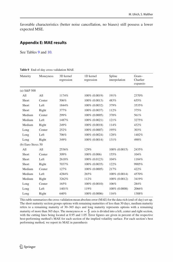
M. Ulrich, S. Walther
favorable characteristics (better noise cancellation, no biases) still possess a lowerexpected MSE.
Appendix E: MAE results
See Tables 9 and 10.
Table 9 End-of-day cross-validation MAE
Maturity Moneyness 3D kernelregression
1D kernelregression
Splineinterpolation
Gram–Charlierexpansio
(a) S&P 500
All All 1174% 100% (0.0019) 191% 2370%
Short Center 506% 100% (0.0013) 483% 655%
Short Left 1844% 100% (0.0032) 379% 3535%
Short Right 377% 100% (0.0037) 112% 375%
Medium Center 299% 100% (0.0005) 370% 561%
Medium Left 1487% 100% (0.0021) 121% 3275%
Medium Right 249% 100% (0.0018) 114% 432%
Long Center 252% 100% (0.0007) 195% 303%
Long Left 706% 100% (0.0024) 128% 1402%
Long Right 349% 100% (0.0014) 131% 490%
(b) Euro Stoxx 50
All All 2536% 129% 100% (0.0015) 2435%
Short Center 309% 100% (0.006) 155% 104%
Short Left 2618% 100% (0.0123) 104% 1184%
Short Right 7037% 100% (0.0035) 122% 9905%
Medium Center 127% 100% (0.0005) 217% 422%
Medium Left 4284% 265% 100% (0.0014) 4570%
Medium Right 3262% 112% 100% (0.0012) 3419%
Long Center 165% 100% (0.0010) 106% 284%
Long Left 1401% 119% 100% (0.0008) 2066%
Long Right 640% 100% (0.0006) 116% 1388%
This table summarizes the cross-validationmean absolute error (MAE) for the data-rich (end-of-day) set-up.The short maturity section groups options with remaining maturities of less than 30 days, medium maturityrefers to a remaining maturity of 30–365 days and long maturity represents options with a remainingmaturity of more than 365 days. The moneyness m = K
F axis is divided into a left, center and right section,with the cutting lines being located at 0.95 and 1.05. Error figures are given in percent of the respectivebest-performing method’s MAE for each section of the implied volatility surface. For each section’s bestperforming method, we report its MAE in parenthesis
123
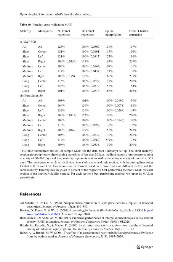
Option-implied information: What’s the vol surface got to…
Table 10 Intraday cross-validation MAE
Maturity Moneyness 3D kernelregression
1D kernelregression
Splineinterpolation
Gram–Charlierexpansion
(a) S&P 500
All All 123% 100% (0.0309) 139% 137%
Short Center 121% 100% (0.0191) 117% 156%
Short Left 121% 100% (0.0813) 155% 116%
Short Right 100% (0.0254) 117% 163% 239%
Medium Center 103% 100% (0.0164) 107% 135%
Medium Left 117% 100% (0.0437) 171% 131%
Medium Rght 100% (0.179) 132% 166% 231%
Long Center 115% 100% (0.0229) 147% 208%
Long Left 143% 100% (0.0372) 158% 154%
Long Right 101% 100% (0.0313) 166% 213%
(b) Euro Stoxx 50
All All 108% 101% 100% (0.0199) 139%
Short Center 164% 156% 100% (0.0078) 191%
Short Left 153% 129% 100% (0.0269) 144%
Short Right 100% (0.0114) 122% 136% 206%
Medium Center 108% 108% 100% (0.0145) 170%
Medium Left 113% 100% (0.0299) 130% 132%
Medium Right 100% (0.0149) 129% 155% 241%
Long Center 105% 100% (0.0239) 132% 246%
Long Left 119% 100% (0.0282) 249% 173%
Long Right 108% 100% (0.033) 139% 230%
This table summarizes the out-of-sample MAE for the data-poor (intraday) set-up. The short maturitysection groups optionswith remainingmaturities of less than 30 days,mediummaturity refers to a remainingmaturity of 30–365 days and long maturity represents options with a remaining maturity of more than 365days. The moneyness m = K
F axis is divided into a left, center and right section, with the cutting lines beinglocated at 0.95 and 1.05. Evaluations are performed based on 3 prior trades on different strikes and thesame maturity. Error figures are given in percent of the respective best-performing method’s MAE for eachsection of the implied volatility surface. For each section’s best performing method, we report its MAE inparenthesis
References
Aït-Sahalia, Y., & Lo, A. (1998). Nonparametric estimation of state-price densities implicit in financialasset prices. Journal of Finance, 53(2), 499–547.
Backus, D., Foresi, S., &Wu, L. (2004).Accounting for biases in Black–Scholes. Available at SSRN, https://ssrn.com/abstract=585623. Accessed 29 Apr 2020.
Bahaludin, H., &Abdullah,M. H. (2017). Empirical performance of interpolation techniques in risk-neutraldensity (RND) estimation. Journal of Physics: Conference Series, 819(1), 012026.
Bakshi, G., Kapadia, N., & Madan, D. (2003). Stock return characteristics, skew laws, and the differentialpricing of individual equity options. The Review of Financial Studies, 16(1), 101–143.
Beber, A., &Brandt,M.W. (2006). The effect of macroeconomic news on beliefs and preferences: Evidencefrom the options market. Journal of Monetary Economics, 53(8), 1997–2039.
123

M. Ulrich, S. Walther
Bliss, R. R., & Panigirtzoglou, N. (2002). Testing the stability of implied probability density functions.Journal of Banking & Finance, 26(2–3), 381–422.
Bollerslev, T.,&Todorov,V. (2011). Tails, fears, and risk premia.The Journal of Finance, 66(6), 2165–2211.Buss, A., & Vilkov, G. (2012). Measuring equity risk with option-implied correlations. The Review of
Financial Studies, 25(10), 3113–3140.Chang, B. Y., Christoffersen, P., Jacobs, K., & Vainberg, G. (2012). Option-implied measures of equity risk.
Review of Finance, 16(2), 385–428.Christoffersen, P., Feunou, B., Jeon, Y., &Ornthanalai, C. (2017). Time-varying crash risk: The role of stock
market liquidity. Rotman School of Management Working Paper No. 2797308. Available at SSRN,https://ssrn.com/abstract=2797308.
Corsi, F. (2009). A simple approximate long-memory model of realized volatility. Journal of FinancialEconometrics, 7(2), 174–196.
Damghani, B. M. (2015). Introducing the implied volatility surface parametrization (IVP): Application tothe FX market. Wilmott, 2015(77), 68–81.
Damghani, B. M., & Kos, A. (2013). De-arbitraging with a weak smile: Application to skew risk. Wilmott,64, 40–49.
Drechsler, I., & Yaron, A. (2011). What’s vol got to do with it. The Review of Financial Studies, 24(1),1–45.
Driessen, J., Maenhout, P. J., & Vilkov, G. (2009). The price of correlation risk: Evidence from equityoptions. The Journal of Finance, 64(3), 1377–1406.
Du, J., & Kapadia, N. (2012). Tail and volatility indices from option prices. https://people.umass.edu/nkapadia/docs/Du_Kapadia_August2012.pdf. Accessed 29 Apr 2020.
Fengler, M. R. (2009). Arbitrage-free smoothing of the implied volatility surface. Quantitative Finance,9(4), 417–428.
Figlewski, S. (2008). Estimating the implied risk neutral density. In M. W. Tim Bollerslev & J. R. Russell(Eds.), Volatility and time series econometrics: Essays in honor of Robert F. Engle. Oxford: OxfordUniversity Press.
Gatheral, J. (2004). A parsimonious arbitrage-free implied volatility parameterization with application tothe valuation of volatility derivatives. In Presentation at Global Derivatives & Risk Management,Madrid. http://faculty.baruch.cuny.edu/jgatheral/madrid2004.pdf. Accessed 29 Apr 2020.
Gatheral, J. (2006). The volatility surface: A practitioner’s guide. Hoboken, New Jersey: Wiley.Geisser, S. (1993). Predictive inference: An introduction. Monographs on statistics and applied probability
(1st ed., p. 55). New York: Chapman & Hall.Hagan, P. S., Kumar, D., Lesniewski, A. S., & Woodward, D. E. (2002). Managing smile risk. The Best of
Wilmott, 1, 249–296.Heston, S. L. (1993). A closed-form solution for options with stochastic volatility with applications to bond
and currency options. The Review of Financial Studies, 6(2), 327–343.Hofmann, M., & Uhrig-Homburg, M. (2018). Volatility noise. Available at SSRN, https://ssrn.com/
abstract=3130045. Accessed 29 Apr 2020.Hull, J. (2018). Options, futures, and other derivatives (10th ed.). New York, NY: Pearson.Jackwerth, J. C. (1999). Option-implied risk-neutral distributions and implied binomial trees: A literature
review. The Journal of Derivatives, 7(2), 66–82.Jackwerth, J. C. (2000). Recovering risk aversion from option prices and realized returns. The Review of
Financial Studies, 13(2), 433–451.Jackwerth, J. C., & Rubinstein, M. (1996). Recovering probability distributions from contemporaneous
security prices. The Journal of Finance, 51(5), 1611–1631.Jiang, G. J., & Tian, Y. S. (2005). The model-free implied volatility and its information content. The Review
of Financial Studies, 18(4), 1305–1342.Jondeau, E., & Rockinger, M. (2000). Reading the smile: The message conveyed by methods which infer
risk neutral densities. Journal of International Money and Finance, 19(6), 885–915.Kohavi, R. (1995). A study of cross-validation and bootstrap for accuracy estimation and model selection.
Proceedings of the Fourteenth International Joint Conference on Artificial Intelligence, 14(2), 1137–1145.
Martin, I.W.R., (2017). What is the expected return on the market? The Quarterly Journal of Economics,132(1), 367–433.
Martin, I., & Wagner, C. (2019). What is the expected return on a stock? The Journal of Finance, 74(4),1887–1929.
123

Option-implied information: What’s the vol surface got to…
OptionMetrics (2016). IvyDB US File and Data Reference Manual, Version 3.1, Rev. 8/19/2016. 1776Broadway, Suite 1800, New York, NY 10019.
Schneider, P., &Trojani, F. (2015). Fear trading Swiss Finance Institute Research PaperNo. 15-03. Availableat SSRN, https://ssrn.com/abstract=1994454.
Schönbucher, P. J. (1999). A market model for stochastic implied volatility. Philosophical Transactionsof the Royal Society of London Series A: Mathematical, Physical and Engineering Sciences, 357,2071–2092.
Swanson. E. T. (2016). Discussion of options-implied probability density functions for real interest rates.http://www.ijcb.org/journal/ijcb16q3a3_disc.pdf.
Wright, J. H. (2016). Options-implied probability density functions for real interest rates. InternationalJournal of Central Banking, 12(3), 129–149.
Zhao, B., & Hodges, S. D. (2013). Parametric modeling of implied smile functions: A generalized SVImodel. Review of Derivatives Research, 16(1), 53–77.
Publisher’s Note Springer Nature remains neutral with regard to jurisdictional claims in published mapsand institutional affiliations.
123