Imputed Welfare Estimates in Regression Analysis1

Chris Elbers2 Jean O. Lanjouw3 Peter Lanjouw4

September 4, 2003

1We thank Ravi Kanbur, Tony Venables and other participants at the WIDERproject meeting on Spatial Inequality in Development, May 2003, for comments onan earlier draft of this paper.

2Amsterdam Institute for International Development; and Vrije Universiteit Am-sterdam, celbers@feweb.vu.nl.

3ARE Department, U.C. Berkeley, Brookings Institution and the Center forGlobal Development, Washington, DC, jlanjouw@brook.edu.

4World Bank, Washington, DC, planjouw@worldbank.org. Financial supportwas gratefully received from the Bank Netherlands Partnership Program. None ofthe views expressed here should be taken to represent those of the World Bank oraffiliated organizations.

Abstract

We discuss the use of imputed data in regression analysis, in particularthe use of highly disaggregated welfare indicators (from so-called ‘povertymaps’). We show that such indicators can be used both as explanatory vari-ables ‘on the right hand side’ and as the phenomenon to explain, ‘on theleft hand side’. We try out practical ways of adjusting standard errors ofthe regression coefficients to reflect the error introduced by using imputed,rather than actual, welfare indicators. These are illustrated by regressionexperiments based on data from Ecuador. For regressions with imputedvariables on the left hand side we argue that essentially the same aggregaterelationships would be found with either actual or imputed variables. Weaddress the methodological question of how to interpret aggregate relation-ships found in such regressions.

Introduction

The growing access of researchers to household data makes possible the esti-mation of inequality and poverty measures at very disaggregated levels. InElbers, Lanjouw and Lanjouw (2003) we describe a procedure that combinesthe broad coverage of a census or large survey and the detail of householdsurvey data to arrive at estimators that are quite precise - comparing veryfavorably to estimates based on either source alone. Using this strategy, es-timates of local welfare (so-called ‘poverty maps’) have been constructed formany countries (see Demombynes, et al., 2003, for examples). These mapsprovide useful information about the geographic spread of relative povertyand inequality that can be directly useful to policy makers pursuing povertyalleviation or development goals.

In addition to their direct informational use, the imputed welfare esti-mates also provide a wealth of distributional information that could be usedin economic analysis. Theories abound regarding what causes localities tobe poor or unequal and how these characteristics might affect other social oreconomic outcomes. In the absence of appropriate data it has been difficultto explore these ideas empirically. Imputed welfare estimates could enablemore extensive applied distributional analysis. In such studies, however, itwill be important to take account of the fact that the estimates are exactlythat, estimates, and not data. Thus, in this paper we discuss the economet-ric issues raised when using imputed welfare estimates in regression analysis- as either a dependent variable or an explanatory variable.

Most of the issues we discuss are quite general and arise in all situationsusing predicted variables. An extensive discussion, for example, can befound in Murphy and Topel (1985). We focus here on the use of imputedwelfare variables. We make suggestions regarding some particular problemsthat might arise when using these variables, and explore the importance ofvarious issues using Ecuador as an illustration.

Specifically, we are interested analyzing the relationships between a truewelfare measure, W , and other variables in what we will call ‘downstream’regressions. W is unknown but we have consistent estimates of the expectedvalue of W denoted by µ. The estimate µ is an error ridden variable. How-ever, by its construction it can be understood as an instrumented versionof W and standard results, including consistency, for IV estimators obtain.Although the welfare estimates are more complex than standard instumen-tal variables, we show how one can use information about the distributionof µ to calculate consistent standard errors for the downstream coefficientestimates.

1

Using an imputed value to serve as an explanatory variable may create anendogeneity problem if the variables used in its construction are correlatedwith the disturbance in the downstream regression. We examine the likelyimportance of this concern when the correlated variables and the regressionsare at various levels of aggregation and suggest ways to avoid introducing anendogeity bias. The use of imputed values may also resolve an endogeneityproblem. In some situations the true value of W may be correlated withthe disturbance term. In this case, one would like to instrument W usingvariables uncorrelated with the disturbance in the downstream regression.With attention paid to how they are constructed, predicted values µ can beinterpreted as useful instruments for W when W is endogeneous. That is,predicted values can be superior to the unknown true values W .

The construction of the imputed welfare estimates is briefly described inSection 1. In Section 2 we discuss the use of these estimates as an explana-tory variable and in Section 3 describe practical approaches to calculatingconsistent standard errors for the downstream regression coefficients. Endo-geneity issues are considered in Section 4. In Section 5 we discuss the use ofan imputed value as the dependent variable in the downstream regression.The last section concludes.

1 Calculation of Imputed Welfare Estimates

Denote by W a measure of poverty or inequality based on the distributionof a household-level variable of interest, yh, for instance per-capita expen-diture. Data on yh as well as a number of covariates zh are available froma household survey, where h refers to a household included in the surveyand bold variables indicate vectors and matrices. Measuring household per-capita expenditure reliably is very costly, therefore this kind of survey istypically only representative at high levels of aggregation, say the provincelevel. Consequently, welfare indicators W , based on direct observations ofy, are also at best available at the province level. By bringing in informa-tion from other data sources we can overcome this limit and compile welfareestimates at levels of aggregation far below the province level.

The idea is that from the household survey we can estimate the jointdistribution of yh and one or more of the covariates zhi. Assume that alarger-scale sample or a census of households is available, held at aboutthe same time as the survey and containing observations of some of thecomponents of zh. By estimating the joint distribution of yh and the subset

2

of covariates also in the census,1 this estimated distribution can be used togenerate the distribution of yh for any sub-population in the larger sampleconditional on the sub-population’s observed characteristics. This, in turn,allows us to generate the conditional distribution of W for sub-populations.We do this by means of simulation.

In what follows we let z denote the vector of covariates which can belinked to both survey and census households. The first step, which we callthe ‘first stage’, is to develop an accurate empirical model of ych, the per-capita expenditure of household h in sample cluster c. Typical applicationshave used a log-linear approximation to the conditional distribution of ych,

ln ych = E[ln ych|zch] + uch ≈ z′chγ + ηc + εch. (1)

By including cluster random effects ηc in the equation we allow for a withincluster correlation of disturbances uch. The error components η and ε areassumed to be independent of each other. They are uncorrelated with ob-servables, zch, by construction.

Suppose that there are M households in a target population and house-hold h has mh family members. In general one will want to account forhousehold size in welfare measures, so we write W (m,Z,γ,u), where m,Z and u are conformable arrays of household size, observable characteris-tics and disturbances, respectively. The expected value of W given theobservable characteristics and the model of expenditure is denoted µ =E[W |m,Z, ζ], where ζ is the vector of model parameters, including γ andany parameters describing the distribution of the disturbances η and ε.

In the second stage construction of our estimator of µ we replace ζ withconsistent estimators, ζ, from the first stage expenditure regression. Simu-lation is used to obtain µ =E{E[W | m,Z,ζ]}, where the outer expectationis over the sampling distribution of ζ, given ζ = ζ.

The difference between µ, the estimator of the expected value of W fora population, and the actual level may be written

ξ = W − µ = (W − µ) + (µ− µ). (2)

Thus the prediction error ξ has two components:2

1Actually, we can do better than that. We can bring in any variable that can belinked both to survey and census households. In practice this appears to be a crucialimprovement. See Elbers et al. (2003) for details.

2There is also simulation error, but we will assume that it has been made small enoughto ignore.

3

Idiosyncratic Error - (W − µ). The actual value of the welfare indicatorfor a population deviates from its expected value, µ, as a result ofthe realizations of the unobserved component of expenditure. Thiscomponent increases as one focuses on smaller target populations.

Model Error - (µ−µ). This component of the prediction error is determinedby the properties of the first-stage estimators so it does not increaseor fall systematically as the size of the target population changes.

Elbers, Lanjouw and Lanjouw (2003) show that these error componentsare asymptotically normal, converging in the population size M and thehousehold survey size s. In typical applications the overlap between thetarget population and the survey is virtually nil, so the variance of the totalprediction error is the sum of individual error variance components:

V = VI + VM. (3)

2 Predicted Welfare as an Explanatory Variable

Consider first using imputed welfare measures on the ‘right hand side’ of aregression. Start from the general regression equation

D = x′α +Wβ + τ. (4)

D is explained by regressor vector x and welfare indicator W . We areinterested in estimating β, the effect of W on D. In our case W is notobserved, so we use estimates of expected welfare µ. As discussed above,our predicted welfare is related to W as

W = µ+ ξ. (5)

Substituting this equation in the regression equation one gets

D = x′α + µβ + (ξβ + τ). (6)

It follows that β can be consistently estimated if x and µ are uncorrelatedwith ξ and τ , or if µ is uncorrelated with x, ξ, and τ .

In our case, µ is a consistent estimator of the conditional expectation ofW , ξ is a prediction error and so µ and ξ are uncorrelated. Thus, if theother standard properties are met, using µ in a regression rather than Wstill yields consistent estimates.

4

Note the importance of the fact that µ is a prediction. If instead µwere some other proxy for W , then the error ξ would represent a form ofmeasurement error which is correlated with µ. It is possible that an analystmight inadvertently introduce measurement error into the regression whenW is a discrete variable (say, poverty status at the household level). Becauseits expectation, µ = E(W |z), is a continuous variable (expected povertystatus given household characteristics z) it is tempting in this circumstanceto use a discrete version of µ, say W , in equation (6) ( i.e. setting W = 1 for ahousehold if µ ≥ 0.5 and 0 otherwise). This would not be advisable becausemeasurement error typically leads to attenuation bias in the estimation ofβ.

2.1 Standard errors on downstream regression coefficients

When using imputed welfare as an explanatory variable in a regression equa-tion, the estimated standard errors on the regression cofficients must takeaccount of additional noise in the estimates. To see this, insert equation (2)into regression equation (4) to obtain

D = x′α + µβ + (µ− µ)β + (W − µ)β + τ. (7)

The error term ψ in this regression consists of the following components

ψ = (µ− µ)β + (W − µ)β + τ. (8)

Thus there are three sources of error in the estimates of the downstreamregression coefficients of equation (7). One is the standard sampling error(represented by τ), a second derives from the difference between W andthe true expectation µ (the idiosyncratic error), and the third is from thedifference between µ and its estimate µ (the model error). Except for theidiosyncratic error part (W − µ)β this error decomposition is very similarto formula (8) in Murphy and Topel (1985). As in their case, estimatingequation (7) directly from data on D, x, and µ, would typically underesti-mate the true variance of the estimator for β, because the model error term(µ− µ)β creates correlation across the observations.

The source of correlation is clear. Recall that model error arises be-cause computation of µ requires knowledge of ζ, the parameter vector thatdescribes consumption. As explained in section 1, estimates of these pa-rameters are used to impute (the conditional distribution of) consumptionexpenditure for all households in a target population. Because the sameexpenditure model is applied to a group of households the same (erroneous)

5

parameter estimates are applied to all of them, thus creating correlationacross errors in the prediction of those households’ consumption expendi-ture. This correlation is very likely to carry over to higher levels of aggre-gation (sub-district, district, and so on).3

It is nonetheless straightforward to estimate the full variance of the esti-mated parameters α and β of the regression equation (7) once the correlationof the model error across downstream observations is known. To see this,rewrite the regression equation as

D = Xλ + (µ− µ)β + e,

where X is the matrix of observations (x, µ), λ = (α, β) is the vector of re-gression parameters, and e = (W − µ)β + τ is the residual part not relatedto model error. ΣM is the covariance matrix of model error in µ. If thecomponents of e are i.i.d. and there are no endogeneity issues plaguing theregression, then OLS is unbiased and the variance of the OLS estimator4 forλ is

Var(λ) = σe(X

′X)−1 + β(X′X)−1X′ΣMX(X′X)−1. (9)

Below we will refer to the first term in (9) as the ‘sampling’ part of thevariance and the second part as the ‘model’ part of the variance. In thenext section we try out alternative ways to compute Var(λ).

3 Estimation of standard errors

Suppose, first, that one knew the true expected value of W , that is µ = µand ΣM = 0. In this case, the second term of Var(λ) in equation (9) woulddisappear. The downstream regression model (7) and standard errors couldbe estimated in the usual way. The only complication would come fromthe fact that households within the same cluster share a common locationeffect which affects their consumption level in a similar way (the disturbancecomponent ηc in equation 1). Thus the idiosyncratic part of the predictionerror (W - µ)β is correlated when observations are at the level of households.5

In spite of this complication, the sampling part of the variance in λ canbe estimated consistently at the household level using standard methods.

3Typically it is possible to estimate separate consumption models at the level of strata.Estimates for sub-populations belonging to different survey strata then do not have cor-related model error.

4Although a feasible GLS estimator would be more appropriate in this case and istypically used in applications, we do not discuss it in this paper.

5The prediction errors might also be heteroscedastic, although in our experience thevariance of µ does not appear related to its size, as one might have expected.

6

One approach is to estimate the model with µ and then use downstreamregression residuals and a robust variance formula (see, for example, Greene(2000), equation 11-14). With large numbers of downstream observations,however, this is cumbersome. Alternatively one could bootstrap the vari-ance by resampling out of the downstream data (including µ), re-estimatingthe model many times, and calculating the variance of the resulting esti-mates of λ.6 By bootstrapping, any correlation in the idiosyncratic erroracross observations due to location effects is incorporated in the varianceestimation directly. Note that, in general, if the downstream regressionis estimated at a level of aggregation higher than the level of any locationeffects then the prediction errors (W-µ) are no longer correlated and thesesteps are unnecessary.

We now turn to estimation of the second term in (9), the variance dueto model error in the imputed welfare estimates. From our earlier discus-sion, recall that ζ denotes the true parameter vector underlying expenditureequation (1), and write µ = µ(ζ) to stress the dependency of µ on ζ. Fol-lowing Murphy and Topel we could relate the model error µ− µ to the errorin ζ by linear approximation:

µ−µ ≈ ∂µ

∂ζ(ζ)(ζ−ζ)

and use the estimated variance of ζ to infer the (asymptotic) error dis-tribution of µ.7 However, for the purpose of calculating the variance indownstream regression coefficients the simplest approach is to simulate thedistribution of µ− µ directly (see below, section 3.1). Bypassing the calcu-lation of derivatives has the additional advantage that (small-sample) biasarising from the linear approximation in Murphy and Topel’s approach isavoided.

The simulations are described in the following subsection. They are doneunder the assumption that there is no correlation between the model errorpart (µ − µ)β and the other components of equation (8), (W − µ)β + τ .8

The main justification for this assumption is that the model error µ − µis ultimately caused by sampling variation in the survey from which ζ is

6The bootstrapping should be nested like the error structure in equation (1) by firstdrawing groups of households at the level of aggregation where ηc applies, and then draw-ing households randomly within the group.

7See Murphy and Topel (1985), page 374. This approach is taken in Elbers, Lanjouwand Lanjouw (2003).

8In the terminology of Murphy and Topel this is the case of independent random com-ponents.

7

estimated. This survey typically covers only a tiny fraction of the populationfor which the welfare indicators µ have been compiled and may come froma different time period.

To perform the calculations described in subsection 3.1 below one needsto employ the data that were used in the computation of the estimatorsµ. Since most researchers will not have access to the unit record level data,particularly not for a census, we propose in subsection 3.2 several alternativeways to approximate ΣM when pieces of information are unknown. Ulti-mately our goal is to find a parsimonious and satisfactory representationof ΣM which could be reported together with the welfare estimates in apoverty mapping project so that analysts can readily adjust standard errorsfrom regressions involving imputed welfare estimates. In the final subsectionwe give empirical illustrations for Ecuador.

3.1 Estimation with unit record data

The model error part in the variance of λ, i.e. the second term in (9) isdue to error in the consumption model used to estimate µ. The combinedeffect of sampling and model error can be simulated by drawing from thedistribution of µ and e and re-estimating the downstream regression model.As discussed in Section 1, the estimates µ are determined by householdsurvey data and a vector of estimated consumption model parameters ζ. Inthe simulations we take the following steps:

1. Draw vectors ζr, r = 1, ..., R, from the appropriate sampling distri-

bution (see Elbers, et al., 2003, for this distribution).

2. Simulate the expected welfare measures implied by each, µr = µ(ζr).

3. Draw a simulated vector of downstream regression disturbances er

from an estimated distribution of e. Construct a new vector of simu-lated dependent variables Dr = Xλ + er.

4. Estimate the downstream regression coeffient λ using the simulatedDr and Xr, where Xr is the matrix of observations (x, µr).

The variance of these R simulated values λr

gives an estimate of the totalerror variance of λ.9

9The estimator λ is consistent but biased when µ is unknown. The average of the

simulated coefficient estimates λr

derived from this procedure would give an unbiasedestimator under the (estimated) sampling distribution of µ.

8

3.2 Estimation without unit record data

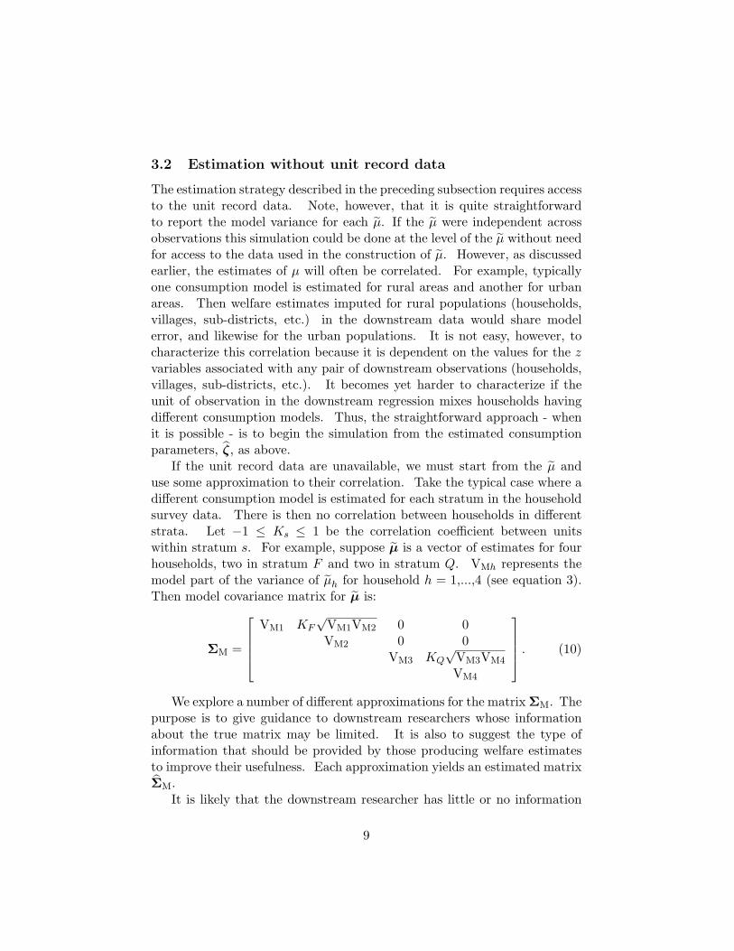
The estimation strategy described in the preceding subsection requires accessto the unit record data. Note, however, that it is quite straightforwardto report the model variance for each µ. If the µ were independent acrossobservations this simulation could be done at the level of the µ without needfor access to the data used in the construction of µ. However, as discussedearlier, the estimates of µ will often be correlated. For example, typicallyone consumption model is estimated for rural areas and another for urbanareas. Then welfare estimates imputed for rural populations (households,villages, sub-districts, etc.) in the downstream data would share modelerror, and likewise for the urban populations. It is not easy, however, tocharacterize this correlation because it is dependent on the values for the zvariables associated with any pair of downstream observations (households,villages, sub-districts, etc.). It becomes yet harder to characterize if theunit of observation in the downstream regression mixes households havingdifferent consumption models. Thus, the straightforward approach - whenit is possible - is to begin the simulation from the estimated consumptionparameters, ζ, as above.

If the unit record data are unavailable, we must start from the µ anduse some approximation to their correlation. Take the typical case where adifferent consumption model is estimated for each stratum in the householdsurvey data. There is then no correlation between households in differentstrata. Let −1 ≤ Ks ≤ 1 be the correlation coefficient between unitswithin stratum s. For example, suppose µ is a vector of estimates for fourhouseholds, two in stratum F and two in stratum Q. VMh represents themodel part of the variance of µh for household h = 1,...,4 (see equation 3).Then model covariance matrix for µ is:

ΣM =

VM1 KF

√VM1VM2 0 0VM2 0 0

VM3 KQ

√VM3VM4

VM4

. (10)

We explore a number of different approximations for the matrix ΣM. Thepurpose is to give guidance to downstream researchers whose informationabout the true matrix may be limited. It is also to suggest the type ofinformation that should be provided by those producing welfare estimatesto improve their usefulness. Each approximation yields an estimated matrixΣM.

It is likely that the downstream researcher has little or no information

9

about the differing degrees of correlation in model error across units. Thuswe try to approximate these values with correlation coefficients that areconstant within a given stratum (the Ks). If the welfare estimates arecoming from secondary sources, the researcher also may know only the totalvariance in µ, V, and not the portion due to model error. In this case asecond approximation is needed, with VM = GV. Reasonable values for Kand G will depend on the level of aggregation of the µ.

In the following subsection we present examples from Ecuador. Theseshow the importance of including the model part of Var(λ), and indicatehow sensitive estimates of the variance are to assumptions about the degreeof correlation in the imputed welfare estimates, µ. As will become clearfrom that discussion, the approximations outlined above do not performparticularly well. An alternative would be to replace ΣM in equation (9) bya diagonal matrix ρI for sufficiently high ρ. The model error variance partthen simply becomes

ρβ2(X′X)−1.

For ρ we have used the maximum total variance, V, found among welfareestimates at the level used in the downstream regression.

Finally, one way to assess the possibilities for a parsimonious represen-tation of ΣM is to see how many terms in a singular value decomposition ofit are needed. Results are summarized in Tables 1 and 2 below.

3.3 Experiments for Ecuador

Our empirical examples use data from Ecuador. Expected welfare is basedon household per-capita expenditure. Consumption models are estimatedusing the 1994 Ecuadorian Encuesta Sobre Las Condiciones de Vida, ahousehold survey following the general format of a World Bank Living Stan-dards Measurement Survey. It is stratified by 8 regions and separate modelsare estimated for each stratum. We were able to capture most of the effect oflocation on consumption with available explanatory variables. This meansthat there is little correlation across households in their idiosyncratic error.The models are used to impute welfare measures for target populations inthe 1990 Ecuadorian census.(See Elbers, Lanjouw, and Lanjouw, 2002, fora full discussion of the estimation procedure and diagnostics.)

We study canton-level regressions where the dependent variable is ‘garbage’,the percentage of households in the canton whose garbage is collected bythe municipal trucks.10 The explanatory variables are a normalized mea-

10The available levels of aggregation are (in increasing order of aggregation) household,

10

sure of cantonal population size and a point estimate of welfare, either thelocal headcount or the local inequality index GE(0.5). Moreover, provincedummies have been added to avoid obvious omitted variables bias. The es-timations use pooled data for the Rural Costa and Sierra regions for a totalof 164 cantons with an average population of 26650.

[INSERT TABLE 1 HERE]

The regression results are reported at the top of Tables 1 and 2, respec-tively, where the reported standard errors reported in the top panel of thetable include only the sampling part of the error. Local poverty is associ-ated with a lower incidence of garbage collection, while greater communityinequality is associated with a higher level of service. Both regressions havereasonable R2s, given that these are cross-section regressions. The coeffi-cients on the province dummies are not reported. Each of these dummies ishighly significant in both regressions. On the other hand, without the dum-mies the parameter estimates and significance levels of the welfare indicatorsare very similar to the values reported in Tables 1 and 2.

The bottom part of each table shows the additional error in the welfarecoefficient due to the fact that welfare levels - either poverty or inequality- have been imputed. The first row gives the results obtained when fullinformation about ΣM can be determined from the unit record data. We usethe empirical covariance matrix derived from 100 simulated sets of welfareindicators. Consider first Table 1. Column (1) gives the additional variance- the (‘µ’, ‘µ’) component of the matrix β2(X′X)−1X′ΣMX(X′X)−1. Thestandard error is in column (2) and one can see that it is about 5% of thevalue of the coefficient estimate. The third column gives the full variance(8.959 plus column 1) with the full standard error in column 4. Columns(5) and (6) indicate the share of the model variance in the total variance,and what it represents as a percentage increase, respectively. At over 9%the addition to the variance in the downstream regression coefficient on theheadcount due to the fact that it is estimated is not trivial. However, thecoefficient is still clearly significant.

The next four lines in the table explore different ideas for approximatingthe model covariance matrix ΣM. The results are negative; these simpleapproximations to the covariance matrix simply do not work, and our questfor a parsimonious approximation to ΣM will have to continue.

parroquia, canton, province, and region.

11

In each case we approximate G, discussed in section 3.2, by taking theshare of model error in the variance of the total prediction error in µ, VM

V ,and averaging it over cantons. This gives 0.92 for Rural Costa and 0.66for Rural Sierra. These numbers are high because idiosyncratic error di-minishes in importance at the canton level due to aggregation. Each rowmakes a different assumption about the degree of correlation, K, betweenestimates of the expected headcount across cantons within each of the twostrata. Clearly in this model using a single value to summarize the correla-tion leads to underestimation of the model error component - for any valueof K between 0 and 1. Note that the underestimation gets worse if oneallows for more (average) correlation. These results are not general: in aregression without province dummies the approximated model error compo-nent increases with correlation and the model error effect is well reproducedfor average correlation of K = 0.15.

The last two lines show that a crude error approximation (see section3.2) with ρ equal to the maximum among all prediction error variances, V,gives a safe but rather high upper bound to the model part of the variancein β. Also, the first twenty terms in a singular value decomposition of ΣM

suffice to accurately replicate the model error-induced error on the head-count coefficient. This is some, but not a big gain compared to needing thefull ΣM matrix.

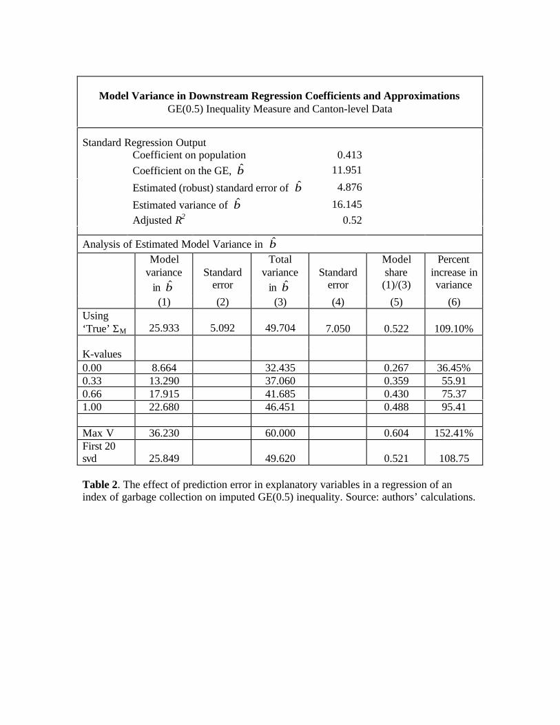
[INSERT TABLE 2 HERE]

In Table 2 we see that the fact that the welfare variable is imputedmakes considerably more difference when it is an indicator of inequality.There are two reasons for this. First, the unadjusted regression results in amuch lower significance level for the coefficient on the welfare indicator andsecond, the prediction error on the inequality measure is much bigger thanthat of the headcount. On average the prediction (standard) error is 11.7%for the inequality measure and 4.2% for the headcount. Thus, inclusion ofthe model error in β increases its variance by more than 100%. We seethat the coefficient on inequality, which appeared to be significant whenmodel error was ignored, is in fact borderline significant at a 10% level (thet-statistic is 1.70). Looking further down the table, we find again that usinga single value to summarize the correlation across welfare estimates leads tounderestimation of the model error component for any value of K between

12

0 and 1.11 However, in this regression the approximation improves if oneallows for more correlation.. The crude error estimation (Max V) gives a veryhigh upper bound in this case and would lead one to (incorrectly) soundlyreject a relationship between inequality and garbage collection services.

4 Endogeneity

In this section we discuss two types of endogeneity issues.

4.1 Endogeneity of W

True welfare W may be correlated with the regression disturbance τ . In thiscase, one would like to instrument for W , and µ may be a better explanatoryvariable to use in the downstream regression even if W were known.

Example one - Health: Suppose that a health indicator of interest isindependent of inequality but both are correlated with an omitted variable‘ethnic diversity’. Estimating the health regression with true inequalitywould give a positive, but spurious, coefficient.

Example two - Credit: Suppose that credit availability is independentof poverty but both are correlated with an omitted variable ‘remoteness’. Inthis situation we would find a negative coefficient onW in a credit regression,but again it would be spurious.

Using µ instead of W resolves this type of endogeneity problem.

4.2 Endogeneity of µ

As in any problem involving instrumental variables, using predicted valuesmay create, rather than resolve, an endogenity problem. However, it isimportant to realize that when µ is correlated with the downstream dis-turbance τ, the (unknown) true value of welfare, W , would likely also becorrelated with the disturbance. There would indeed be an endogeneityproblem, but not one special to having used a predicted value for welfare.The only cause for additional concern then, would be if by contruction µwas correlated with τ when W itself was not.

One plausible way to have a regression in which expected welfare is corre-lated with the disturbance is if one of the variables used in the construction

11The table reports results for the (extreme) assumption that all prediction error ismodel error, or G = 1.

13

of µ should have been included in the downstream regression but is omitted.That said, note that while the suspect variable would have entered the re-gression, say, linearly, it enters µ ‘mixed’ in a non-linear fashion and possiblyat a different level of aggregation. So it is not obvious whether the effect ofthe omitted variable would be picked up on µ in the downstream regression.Thus the first question we ask is whether or not, given this ‘mixing’, thereremains any correlation between estimated welfare and the variables that gointo its construction. If not, then leaving the variables used to construct µout of the downstream regression, even when those variables are related toD, will not bias the coefficient on expected welfare.

An investigation of the correlation between selected household-level vari-ables used in the consumption model and the resulting estimates of expectedwelfare is presented in Table 3.

[INSERT TABLE 3 HERE]

The first column gives the measure, either the poverty headcount orthe GE (0.5) measure of inequality. The second column shows the levelof the explanatory variables, i.e. ‘Parroquia’ indicates that the variablesare means at that level of aggregation. The third column gives the levelof aggregation for the welfare estimate, µ. The rest of the columns givecorrelation coefficients between µ and the variable indicated in the columnheading. These are fairly self-explanatory except for the last three whichare a set of dummy variables for the type of sanitation in the householdresidence.

Several points emerge. First, there is far less correlation between the µand other variables when µ is an inequality measure. This is not surprisingas inequality is particularly non-linear. With a household-level regression,in fact, the ‘mixing’ seems to remove almost all correlation. In househouldregressions, then, it seems extremely unlikely that including a constructedestimate of inequality will create any endogeneity issues.

Second, in many cases we do see considerable correlation. In these situ-ations the best advice would be to include both µ and the suspect variablesin the downstream regression if possible. Again, we emphasize that this isnot special to using a predicted variable and is likely to be an importantprecaution even if one were to have true W.

Finally, it is interesting to observe that for both poverty and inequality,the correlations get stronger at higher levels of aggregation. Take eduation

14

of the head, for example. Although estimated poverty at the parroquia levelis constructed from household measures of education, it is more strongly cor-related (0-0.32 vs -0.62) with the average level of education for the parroquiathan it is with the household measures used in its construction. There seemto be macro relationships between the variables and the welfare levels thatextend beyond their micro relationship with household consumption. Thesecall for further investigation.

5 Predicted welfare on the LHS

We have seen how imputed welfare estimates can be used in a straightforwardway as explanatory variables. Many questions of interest in development,however, concern the determinants of distributional outcomes. Exploringthese questions requires using imputed variables on the LHS of a regressionand on the face of it this looks suspect. The expenditure equation (1) givesa full statistical description of household level consumption. Given thedistribution of household observables z in the target population, and thedistribution of the error components η and ε the (expected) distribution ofconsumption expenditure is fully determined: there seems to be no roomfor further determination of this distribution. For instance, suppose theexpenditure equation involves a household-level education variable. Thenit would seem to be very suspect to regress canton-level poverty, imputedfrom the expenditure equation, on average education in the canton. Sincethe regression coefficient on average education is completely determined bythe expenditure model and the distribution of education in the population;interpreting it as evidence of a direct relationship, at the aggregate level,seems misleading.

5.1 Analysis

For simplicity, let household per-capita expenditure ykh of household h incanton k be determined by the single variable household-level education zkh

and an i.i.d. error term ukh, uncorrelated with zkh:

ln ykh = zkh + ukh. (11)

15

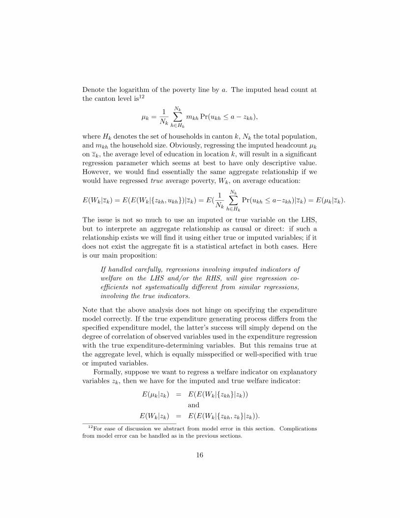
Denote the logarithm of the poverty line by a. The imputed head count atthe canton level is12

µk =1Nk

Nk∑h∈Hk

mkh Pr(ukh ≤ a− zkh),

where Hk denotes the set of households in canton k, Nk the total population,and mkh the household size. Obviously, regressing the imputed headcount µk

on zk, the average level of education in location k, will result in a significantregression parameter which seems at best to have only descriptive value.However, we would find essentially the same aggregate relationship if wewould have regressed true average poverty, Wk, on average education:

E(Wk|zk) = E(E(Wk|{zkh, ukh})|zk) = E(1Nk

Nk∑h∈Hk

Pr(ukh ≤ a−zkh)|zk) = E(µk|zk).

The issue is not so much to use an imputed or true variable on the LHS,but to interprete an aggregate relationship as causal or direct: if such arelationship exists we will find it using either true or imputed variables; if itdoes not exist the aggregate fit is a statistical artefact in both cases. Hereis our main proposition:

If handled carefully, regressions involving imputed indicators ofwelfare on the LHS and/or the RHS, will give regression co-efficients not systematically different from similar regressions,involving the true indicators.

Note that the above analysis does not hinge on specifying the expendituremodel correctly. If the true expenditure generating process differs from thespecified expenditure model, the latter’s success will simply depend on thedegree of correlation of observed variables used in the expenditure regressionwith the true expenditure-determining variables. But this remains true atthe aggregate level, which is equally misspecified or well-specified with trueor imputed variables.

Formally, suppose we want to regress a welfare indicator on explanatoryvariables zk, then we have for the imputed and true welfare indicator:

E(µk|zk) = E(E(Wk|{zkh}|zk))and

E(Wk|zk) = E(E(Wk|{zkh, zk}|zk)).12For ease of discussion we abstract from model error in this section. Complications

from model error can be handled as in the previous sections.

16

Hence, if

E(E(Wk|{zkh}|zk)) = E(E(Wk|{zkh, zk}|zk)),then

E(µk|zk) = E(Wk|zk).

In other words, if the information in {zkh|h = 1, . . . , Nk} includes the in-formation in zk, then putting µk or Wk on the LHS essentially makes nodifference. This condition will be satisfied if zk is part of the householdcharacteristics {zkh} or is otherwise a function of these. More generally,if zk does not significantly add explanatory power to household per-capitaconsumption expenditure, beyond the variables zkh, then a regression of Wk

on zk would give essentially the same coefficients as a regression of imputedwelfare µk on zk.

Another way to make this point is to consider the regression of Wk onzk:

Wk = zkβ + εk. (12)

Let Wk = µk + ωk, with ωk the (idiosyncratic) prediction error. It followsthat

µk = zkβ + εk − ωk. (13)

If ωk is uncorrelated with zk the latter regression is no more problematicthan the former.

Correlation between ωk and zk will be negligible if including zk in theconsumption regression (1) does not lead to significant improvement of thefit. This will be the case if the z variables are constructed from census data,or more generally from the same data sources used in the construction of thewelfare indicators. These variables, if not included already, will have beenconsidered for inclusion in the consumption regression so that correlationbetween ωk and zk is unlikely to be a problem.

On the other hand if one has (location) data zk from other sources andthere is no practical way to test how well it would have performed as anadditional explanatory variable in the consumption regression, then correla-tion between zk and ωk in equation (13) might compromise the estimationof β. A solution for this would be to instrument zk with census data.13

13Such instrumenting requires access to census data. However, the target regression willtypically not be at the household level but at higher levels of aggregation for which it maybe easier to obtain the necessary census-based data.

17

Finally, a household level statistical relationship such as the expenditureequation (1) does not preclude the existence of aggregate causal relation-ships. The expenditure model and the information on the distribution ofexplanatory variables in the population (from the census) do allow one topredict statistical relationships at aggregated levels. But as emphasized inElbers, et al., (2003, p. 356) the parameters of the expenditure model mea-sure correlation not causality. The predicted aggregate relationships arebased on these correlations and therefore say nothing about the existenceor non-existence of causal aggregate relationships. The correlations pat-terns found at household level in the survey and census data could very wellhave sprung from an aggregate causal relationship! As always in regressions:caveat emptor. It takes meticulous diagnostics before a regression coefficientcan be interpreted as marginal impact. The use of imputed rather than truevariables does not in any way simplify or compound that basic difficulty.

5.2 Example

Consider a Kuznets-type regression of vk, the variance of log per-capitahousehold consumption in location k on average consumption yk, both esti-mated using the model in equation (11). We take the distribution of boththe education variable zkh and the error term ukh to be normal. Hence wefind

vk = var(zkh) + var(ukh)

yk = ezk+ 12vk .

Assume that both var(zkh) and var(ukh) are heteroskedastic; for the sake ofargument, let both depend on the average level of education:

vk = var(zkh) + var(ukh) = ϕ(zk).

Differentiating, we find

dvk = ϕ′(zk)dzk

dyk = yk(1 +12ϕ′(zk))dzk.

Hence,dvk

dyk=

ϕ′(zk)yk(1 + 1

2ϕ′(zk))

.

The slope of the Kuznets curve is ultimately determined by the heteroskedas-ticity function ϕ(zk). Here we have calculated the slope using imputed vari-ables. The main point to note is that explanation of the Kuznets curve

18

depends on explanation of the function ϕ(zk), which itself has nothing todo with using imputed or true variables. If the use of imputed variables hashelped to obtain more information for the analysis of ϕ(zk), that is only animprovement.

6 Conclusions

Some of the oldest research activities in Development Economics involvethe analysis of distributional indicators in relation to other indicators. TheKuznets curve, relating income inequality to average income level is a famousexample. Another example is the never ending debate on the relationshipbetween inequality and growth, with disagreement both on the sign of therelationship and the direction of causality. One of the main motives behindour ‘poverty mapping’ project was to compile more disaggregate and closelycomparable estimates of distributional measures to begin building a betterempirical foundation for these discussions.

Because the estimated inequality and poverty measures are predictedvalues rather than data, their use in regression analysis requires attentionto econometric issues. We have discussed how imputed distributional indi-cators can be used as explanatory variables in regressions. Our conclusionis that imputed variables on the ‘right hand side’ can be regarded as a spe-cial kind of instrumented variables and, if handled correctly, can be safelyused in estimation. This is demonstrated in regressions using data fromEcuador. In a canton-level regression of garbage collection on imputed head-count poverty the fact that explanatory variables were imputed had a smallbut non-negligible effect on the estimated standard errors of the regressioncoefficients. On the other hand, in a similar regression on local inequalitythe increase in error due to imputation was far greater. These regressionexperiments suggest that alongside with the poverty maps it would be de-sirable to publish data on the correlation of welfare indicators across unitsat various levels of aggregation. Otherwise only very crude and potentiallymisleading conclusions can be drawn about the effect of imputations on es-timation precision. Our (limited) experience suggests that there may be nosimple parsimonious substitutes for full covariance matrices of model errorsat various levels of aggregation and for each welfare indicator reported.

Using imputed variables on the ‘left hand side’ is trickier, but essentiallysuch regressions yield results no different from what would follow from sim-ilar regressions involving the true welfare indicators. However, such regres-sions might suffer from problems of omitted variable bias inherent in using

19

imputed variables. We have discussed ways to avoid such problems.We conclude that the scope for analysis of distributional issues at various

levels of aggregation is vastly expanded by the availability of ‘poverty maps’.

References

[1] Demombynes, Gabriel, Chris Elbers, Jenny Lanjouw, Peter Lanjouw,Johan Mistiaen and Berk Ozler (2003) “Producing an Improved Geo-graphic Profile of Poverty: Methodology and Evidence from Three De-veloping Countries,” WIDER Discussion Paper no. 2002/39. Forthcom-ing in Rolph van der Hoeven and Anthony Shorrocks (eds.) Growth,Inequality and Poverty. (Oxford: Oxford University Press).

[2] Elbers, Chris, J.O. Lanjouw and Peter Lanjouw. (2003) “Micro-LevelEstimation of Poverty and Inequality,” Econometrica. Vol. 71, no. 1, pp.355-64.

[3] (2002).“Micro-Level Estimation of Welfare,” Policy Research Work-ing Paper no. WPS 2911. The World Bank.

[4] Greene, William H. (2000) Econometric Analysis. Fourth Edition. (NewJersey: Prentice-Hall, Inc.)

[5] Murphy, Kevin M. and Robert H. Topel (1985) “Estimation and In-ference in Two-Step Econometric Models,” Journal of Business & Eco-nomic Statistics, Vol. 3, no. 4, pp. 370-79.

20

Model Variance in Downstream Regression Coefficients and ApproximationsHeadcount and Canton-level Data

Standard Regression OutputCoefficient on population 0.332Coefficient on the headcount, β -19.132

Estimated (robust) standard error of β 2.993

Estimated variance of β 8.959Adjusted R2 0.66

Analysis of Estimated Model Variance in βModel

variancein β

Standarderror

Totalvariance

in βStandard

error

Modelshare(1)/(3)

Percentincrease invariance

(1) (2) (3) (4) (5) (6)Using‘True’ ΣM 0.826 0.909 9.786 3.128 0.084 9.22%

K-values0.00 0.416 9.375 0.044 4.64%0.33 0.366 9.325 0.039 4.080.66 0.315 9.274 0.034 3.521.00 0.263 9.222 0.029 2.93

Max V 1.971 10.930 0.180 22.00%First 20svd 0.803 9.762 0.082 8.96

Table 1. The effect of prediction error in explanatory variables in a regression of anindex of garbage collection on imputed headcount poverty. Source: authors’ calculations.

Model Variance in Downstream Regression Coefficients and ApproximationsGE(0.5) Inequality Measure and Canton-level Data

Standard Regression OutputCoefficient on population 0.413Coefficient on the GE, β 11.951

Estimated (robust) standard error of β 4.876

Estimated variance of β 16.145Adjusted R2 0.52

Analysis of Estimated Model Variance in βModel

variancein β

Standarderror

Totalvariance

in βStandard

error

Modelshare(1)/(3)

Percentincrease invariance

(1) (2) (3) (4) (5) (6)Using‘True’ ΣM 25.933 5.092 49.704 7.050 0.522 109.10%

K-values0.00 8.664 32.435 0.267 36.45%0.33 13.290 37.060 0.359 55.910.66 17.915 41.685 0.430 75.371.00 22.680 46.451 0.488 95.41

Max V 36.230 60.000 0.604 152.41%First 20svd 25.849 49.620 0.521 108.75

Table 2. The effect of prediction error in explanatory variables in a regression of anindex of garbage collection on imputed GE(0.5) inequality. Source: authors’ calculations.

Measure Regression µ~ Educhead Agehead Nowife Native Hygn1 Hygn2 Hygn3Headcount Household Household -0.36 <0.01 -0.33 0.14 -0.43 -0.06 0.07

Parroquia -0.32 0.05 0.01 0.26 -0.34 -0.17 0.07Canton 0.20 0.05 <0.01 0.21 -0.22 -0.11 0.02

Parroquia Parroquia -0.62 0.23 0.02 0.32 -0.71 -0.51 -0.03Canton Canton -0.69 0.40 -0.08 0.38 -0.78 -0.57 0.05

GE (0.5) Household Parroquia 0.11 <0.01 0.02 0.05 0.06 0.07 -0.11Canton 0.07 0.01 0.04 0.10 -0.02 0.05 -0.12

Parroquia Parroquia 0.15 0.01 0.17 0.11 0.06 0.13 -0.27Canton Canton 0.08 0.07 0.24 0.15 -0.08 0.19 -0.37

Table 3. Correlations between welfare indicators and household characteristics, used in their construction. Source: authors’calculations using unit records of Ecuador population census, 1990.