Fully efficient estimation ofcoefficients of correlation in the

presence of imputed data

Guillaume Chauvet∗ David Haziza †

January 3, 2011

Abstract

Marginal imputation that consists of imputing items separately, gener-

ally leads to biased estimators of population coefficients of correlation. To

overcome this problem, two main approaches have been considered in the

literature: the first consists of using marginal imputation and use a bias-

adjusted estimator; Skinner and Rao (2002). The second consists of using

an imputation method, which preserves the relationship between variables;

Shao and Wang (2002), who proposed a joint random regression imputation

method that succeeds in preserving the relationships between two variables.

One drawback of the Shao-Wang method is that it introduces an additional

amount of variability (called the imputation variance) due to the random

selection of residuals. As a result, it could lead to inefficient estimators.

Following Chauvet, Deville and Haziza (2010), we propose a balanced joint

random regression imputation that preserves the coefficient of correlation

between two variables, while virtually eliminating the imputation variance.

Results of a simulation study support our findings.

Key words: Balanced imputation; coefficient of correlation; imputation; bootstrap

variance estimation.

∗G. Chauvet, Laboratoire de Statistique d’Enquete, CREST/ENSAI, Campus de KerLann, 35170 Bruz, France†Departement de mathematiques et de statistique, Universite de Montreal, Montreal,

Canada

1

1 Introduction

Single imputation, which consists of replacing a missing value by an artifi-

cial value, is often used in statistical agencies for treating item nonresponse.

The main objective of imputation is to reduce the nonresponse bias, which

requires powerful auxiliary information available for all the sample units (re-

spondents and nonrespondents). Most often, some form of marginal impu-

tation is used. That is, items requiring imputation are treated separately.

For univariate parameters such as population totals (or means), marginal im-

putation leads to asymptotically unbiased estimators provided the assumed

model is correctly specified; e.g., Haziza (2009). In practice, many surveys

use deterministic or random regression imputation, which includes mean im-

putation, ratio imputation and random hot-deck imputation as special cases.

Sometimes, the interest lies in estimating bivariate parameters such as re-

gression and correlation coefficients. While marginal imputation is appropri-

ate for univariate parameters, it may lead to considerably biased estimators

of bivariate parameters. Despite the practical importance of regression and

correlation coefficients, the literature on this topic is quite limited. Santos

(1981) studied the bias of several marginal imputation methods on regres-

sion coefficients in the case of simple random sampling without replacement.

Skinner and Rao (2002) proposed to adjust for the bias at the estimation

stage. They considered the case of common donor imputation (see Section

2) and simple random sampling without replacement and studied the proper-

ties of the bias-adjusted estimator under the so-called nonresponse approach.

Shao and Wang (2002) proposed a joint random regression imputation, which

succeeds in preserving the coefficient of correlation between two items.

2

In this paper, we focus on the finite population coefficient of correlation

between two study variables x and y:

ρxy =t11 − t10t01/N

(t20 − (t10)2/N)1/2 (t02 − (t01)2/N)1/2,

where tkl =∑

i∈U xki y

li, (k, l) ∈ {(1, 0), (2, 0), (1, 1), (0, 1), (0, 2)} and U de-

notes the finite population of size N . For example, t10 =∑

i∈U xi and

t11 =∑

i∈U xiyi.

A sample s is selected from U according to a sampling design p(s). Let

wi = 1/πi be the sampling weight attached to unit i, where πi = P (i ∈ s)

denotes its first-order inclusion probability in the sample. A complete data

estimator of ρxy is the plug-in estimator given by

ρxyπ =t11,π − t10,π t01,π/Nπ(

t20,π − (t10,π)2/Nπ

)1/2 (t02,π − (t01,π)2/Nπ

)1/2 , (1)

where tkl,π =∑

i∈swixki y

li and Nπ =

∑i∈swi denote the design-unbiased (or

p-unbiased) expansion estimators of tkl and N, respectively. Under mild reg-

ularity conditions (e.g., Deville, 1999), the estimator ρxyπ is asymptotically

design-unbiased for ρxy.

In practice, both x and y may be potentially missing and require some

form of imputation. We adopt the following notation: let rxi be a response

indicator attached to unit i such that rxi = 1 if i responds to item x and

rxi = 0, otherwise. Similarly, let ryi = 1 if i responds to item y and ryi = 0,

otherwise. Let x∗i be the imputed value used to replace the missing xi and

y∗i be the imputed value corresponding to the missing yi. Finally, let xi = xi

if rxi = 1 and xi = x∗i if rxi = 0. Similarly, let yi = yi if ryi = 1 and yi = y∗i

if ryi = 0. An imputed estimator of ρxy, based on observed and imputed

3

values, is defined as

ρxyI =t11,I − t10,I t01,I/Nπ(

t20,I − (t10,I)2/Nπ

)1/2 (t02,I − (t01,I)2/Nπ

)1/2 , (2)

where tkl,I =∑

i∈swixki y

li. Thus, obtaining an asymptotically unbiased esti-

mator of ρxy requires determining an asymptotically unbiased estimator of

each term, tkl =∑

i∈U xki y

li, (k, l) ∈ {(1, 0), (2, 0), (1, 1), (0, 1), (0, 2)}. For the

terms t10 and t01 (i.e., the marginal first moments), this can be achieved by

using an appropriate deterministic or random imputation method, whereas

the terms t20 and t02 (i.e., the marginal second moments) require a random

imputation method because deterministic methods tend to distort the second

moment of the variables being imputed. The main difficulty lies in obtaining

an asymptotically unbiased estimator of the cross-product term, t11, which

can be viewed as a measure of the relationship between the study variables

x and y. Marginal imputation, which consists of imputing x and y sepa-

rately, generally distorts the relationship between variables so the resulting

estimator of t11 is generally biased. To overcome this difficulty, two main ap-

proaches may be used: (i) Use marginal imputation (or a variant, see Section

2) and use a bias-adjusted estimator; see Skinner and Rao (2002). (ii) Use a

tailor-made imputation method and use the imputed estimator (1); see Shao

and Wang (2002).

In this paper, the properties of estimators are studied under two dis-

tinct approaches: (i) the Nonresponse Model (NM) approach and (ii) the

Imputation Model (IM) approach. Before describing both approaches, we

introduce further notation. Let x = (x1, ..., xN)′ and y = (y1, ..., yN)′, where

4

xi and yi denote the i-th value corresponding to items x and y, respec-

tively. Let δ = (δ1, ..., δN)′ be the vector of sample selection indicators,

where δi = 1 if unit i is selected in the sample and δi = 0, otherwise. Finally,

let r = (rx1, ..., rxN , ry1, ..., ryN)′ be the vector of response indicators. The

NM and IM approaches are described below:

(i)The NM approach: we make explicit assumptions (called the nonre-

sponse model) about the unknown nonresponse mechanism. Inferences are

made with respect to the joint distribution induced by the sampling design

and the assumed nonresponse model. Let prr = P (rxi = 1, ryi = 1), prm =

P (rxi = 1, ryi = 0), pmr = P (rxi = 0, ryi = 1) and pmm = P (rxi = 0, ryi = 0).

If px = prr + prm denotes the probability of response to item x and

py = prr + pmr denotes the probability of response to item y, note that

prr 6= pxpy, in general. Also, we assume that the sample units respond inde-

pendently of one another.

Under the NM approach and random imputation, we define the conditional

nonresponse bias of ρxyI as BqI(ρxyI) = EqEI ((ρxyI − ρxyπ|x,y, δ, r)|x,y, δ),

where the subscripts q and I denote respectively the unknown nonresponse

mechanism and the imputation mechanism. Conditionally given δ, note that

the complete data estimator ρxyπ is a fixed quantity. To simplify the nota-

tion, we write EI (ρxyI |x,y, δ, r) ≡ ρxyI in the remainder of the paper.

(ii) The IM approach: explicit assumptions about the distributions of the

items of interest, called the imputation model, are made. Unlike the NM

approach, the underlying nonresponse mechanism is not explicitly specified,

5

except that it is assumed to be unconfounded; e.g., Rubin (1976). In this

paper, we consider (deterministic and random) regression imputation, which

is motivated by the following bivariate imputation model:

m :yi = z′iβ +

√viεi

xi = z′iγ +√uiηi,

(3)

where zi is a q-vector of auxiliary variables available for all i ∈ s, β and γ

are two q-vectors of parameters, vi = v(zi) and ui = u(zi) are two known

functions and εi (respectively ηi) is a random term independent of zi with

mean 0 and variance σ2ε (respectively σ2

η). Note that εi and ηi are not inde-

pendent in general, and their covariance is denoted as σεη.

Under the IM approach and random imputation, we define the condi-

tional nonresponse bias of ρxyI as BmI(ρxyI) = Em (ρxyI − ρxyπ|δ, r), where

the subscript m denotes the imputation model (3).

The paper is organized as follows: in Section 2, three versions of the cus-

tomary random-hot deck imputation procedure are first presented. Then,

the resulting imputed estimator of the coefficient of correlation between x

and y is shown to be asymptotically biased for all three versions under ei-

ther the NM approach or the IM approach. Finally, following Skinner and

Rao (2002), we consider a doubly robust bias-adjusted estimator. However,

obtaining a bias-adjusted estimator for more complex imputation procedures

may prove to be difficult. To overcome this difficulty, Shao and Wang (2002)

proposed a joint random regression imputation, which preserves the coeffi-

cient of correlation between x and y. It is described in Section 3.1. In Section

3.2, following Chauvet, Deville and Haziza (2010), we propose a fully effi-

6

cient version of the Shao-Wang procedure, which we call balanced random

regression imputation. Under this procedure, the imputation variance aris-

ing from the random selection of residuals, is eliminated. The algorithm for

performing the proposed balanced imputation procedure is presented in Sec-

tion 3.3. In Section 4, motivated by the reverse framework of Fay (1991) and

Shao and Steel (1999), we propose a bootstrap variance estimator which does

not require re-imputation within each bootstrap sample, unlike the method

advocated by Shao and Sitter (1996). In Section 5, we first compare the

performance of several imputation procedures in terms of relative bias and

relative efficiency. Furthermore, the performance of the proposed bootstrap

variance estimator is studied in terms of relative bias and coverage rate.

Finally, we conclude in Section 6.

2 Bias under random hot-deck imputation

In this section, we study the bias of the imputed estimator ρxyI under ran-

dom hot-deck imputation. We consider three versions of random hot-deck

imputation, which are described in Section 2.1. In Section 2.2, we show that

all these methods lead to biased estimators of a coefficient of correlation, in

general.

2.1 Random hot-deck imputation

In this section, we describe three versions of random hot-deck imputation:

common donor random hot-deck imputation (CDI), which was studied by

Skinner and Rao (2002), marginal random hot-deck imputation (MI) and

hybrid random hot-deck imputation (HI). We introduce further notation: let

7

srr = {i ∈ s : rxi = 1 and ryi = 1}, srm = {i ∈ s : rxi = 1 and ryi = 0},

smr = {i ∈ s : rxi = 0 and ryi = 1} and smm = {i ∈ s : rxi = 0 and ryi = 0}

with respective sizes nrr, nrm, nmr and nmm such that nrr+nrm+nmr+nmm ≡

n, the overall sample size.

Common Donor Random Hot-Deck Imputation:

for i ∈ smr, missing xi is imputed by x∗i = xj, j ∈ srr, such that

P (x∗i = xj) =wj∑

k∈swkrxkryk;

for i ∈ srm, missing yi is imputed by y∗i = yj, j ∈ srr such that

P (y∗i = yj) =wj∑

k∈swkrxkryk;

for i ∈ smm, missing (xi, yi) is imputed by (x∗i , y∗i ) = (xj, yj) , j ∈ srr

such that

P [(x∗i , y∗i ) = (xj, yj)] =

wj∑k∈swkrxkryk

.

Marginal Random Hot-Deck Imputation:

for i ∈ smr, missing xi is imputed by x∗i = xj, j ∈ srr ∪ srm such that

P (x∗i = xj) =wj∑

k∈swkrxk;

for i ∈ srm, missing yi is imputed by y∗i = yj, j ∈ srr ∪ smr such that

P (y∗i = yj) =wj∑

k∈swkryk;

8

for i ∈ smm, missing (xi, yi) is imputed by (x∗i , y∗i ) = (xj, yl) , j ∈

srr ∪ srm and l ∈ srr ∪ smr such that

P [(x∗i , y∗i ) = (xj, yl)] =

wj∑k∈swkrxk

wl∑k∈swkryk

.

Hybrid Random Hot-Deck Imputation:

for i ∈ smr, missing xi is imputed by x∗i = xj, j ∈ srr ∪ srm such that

P (x∗i = xj) =wj∑

k∈swkrxk;

for i ∈ srm, missing yi is imputed by y∗i = yj, j ∈ srr ∪ smr such that

P (y∗i = yj) =wj∑

k∈swkryk;

for i ∈ smm, missing (xi, yi) is imputed by (x∗i , y∗i ) = (xj, yj) , j ∈ srr

such that

P [(x∗i , y∗i ) = (xj, yj)] =

wj∑k∈swkrxkryk

.

Note that HI may be seen as compromise between CDI and MI.

2.2 Bias under the NM approach

In this section, we study the conditional nonresponse bias of ρxyI un-

der the NM approach. The relative conditional nonresponse bias of ρxyI ,

RBqI (ρxyI) = BqI (ρxyI) /ρxyπ, can be approximated by

RBqI (ρxyI).= − (1− h) , (4)

9

provided ρxyπ 6= 0, where

h =

{prr + pmm for CDI and HIprr for MI

If ρxyπ = 0 (i.e, the variables x and y are unrelated), the imputed estima-

tor ρxyI is asymptotically qI-unbiased for ρxyπ, as expected. Expression (4)

shows that the asymptotic bias is always negative. That is, the three ver-

sions of random hot-deck imputation attenuate the relationship between both

items. Also, the bias increases as the response probability to both items, prr,

decreases. For CDI and HI, the asymptotic bias vanishes if prm = pmr = 0,

or equivalently, if srm = smr = ∅. In this case, CDI and HI preserve the

relationships between items x and y since both methods use a single donor

when both items are missing, unlike MI. For MI, the asymptotic bias does

not vanish, even if srm = smr = ∅.

Denote the imputed estimator ρxyI under CDI or HI by ρ(CDI−HI) and by

ρ(MI) under MI. From (4), we obtain∣∣∣∣∣RBqI

(ρ(CDI−HI)

)RBqI

(ρ(MI)

) ∣∣∣∣∣ = 1− pmmpmm + prm + pmr

≤ 1. (5)

Expression (5) shows that the bias occurring under MI is always greater

or equal to the bias occurring under CDI or HI. Hence, MI distorts the

relationship between x and y to a greater extent than CDI or HI.

2.3 Bias under the IM approach

In this section, we study the conditional nonresponse bias of ρxyI under the

IM approach. All three versions of random hot-deck imputation are moti-

vated by (3) with zi = 1 and vi = ui = 1 for all i. The relative conditional

10

nonresponse bias of ρxyI , RBmI (ρxyI) = BmI (ρxyI) /Em (ρxyπ), can be ap-

proximated by

RBmI (ρxyI).= −

(1− h

), (6)

where

h =

{prr + pmm for CDI and HIprr for MI

provided σεη 6= 0, where prr =∑

i∈srr wi/∑

i∈swi and pmm =∑i∈smm wi/

∑i∈swi. If σεη = 0 (i.e, the variables x and y are unrelated),

the imputed estimator ρxyI is mI-unbiased for ρxyπ, as expected. Expression

(6) follows from noting that Em (ρxyI |δ, r).= h σεη

σεσηand Em (ρxyπ|δ)

.= σεη

σεση.

Note that expression (6) is a function of the observed response rates prr and

pmm unlike (4), which depends on the true response probabilities.

2.4 A bias-adjusted estimator

Expressions (4) and (6) suggest the following simple bias-adjusted estimator

denoted by ρaxyI :

ρaxyI = min(

1, h−1ρxyI

). (7)

The bias-adjusted estimator (7) is similar to the bias-adjusted estimator pro-

posed by Skinner and Rao (2002). If ρaxyI ≤ 1 for all samples and sets of

repondents, then it is asymptotically unbiased for ρxy under either the NM

approach or the IM approach. Therefore, it is doubly robust since it can be

justified under either approach. For secondary analysts however, computing

the bias-adjusted estimator may not be an easy task because of its non-

standard form. Also, the bias-adjusted estimator given by (7) was obtained

11

in a relatively straightforward fashion for random hot-deck imputation. For

more general imputation methods (e.g., random regression imputation), ob-

taining a bias-adjusted estimator may prove to be much more complex. To

overcome these issues, Shao and Wang (2002) proposed a joint random re-

gression procedure, which is presented next.

3 Joint random imputation procedures

We first describe the Shao-Wang procedure (Shao and Wang, 2002) in Section

3.1. In Section 3.2, we present a fully efficient version of the Shao-Wang

procedure. The details of the algorithm for performing balanced imputation

are provided in Section 3.3.

3.1 The Shao-Wang procedure

Shao and Wang (2002) showed that marginal random regression imputation

does not preserve the coefficient of correlation between the study variables x

and y. Motivated by (3), they proposed a joint random regression imputation

procedure, which can be described as follows:

(i) for rxi = 0 and ryi = 1 (xi missing, yi observed), we use the imputed

values

x∗i = z′i γr +√uiη∗i ,

where

γr =

(∑i∈s

wirxiu−1i ziz

′i

)−1∑i∈s

wirxiu−1i zixi (8)

12

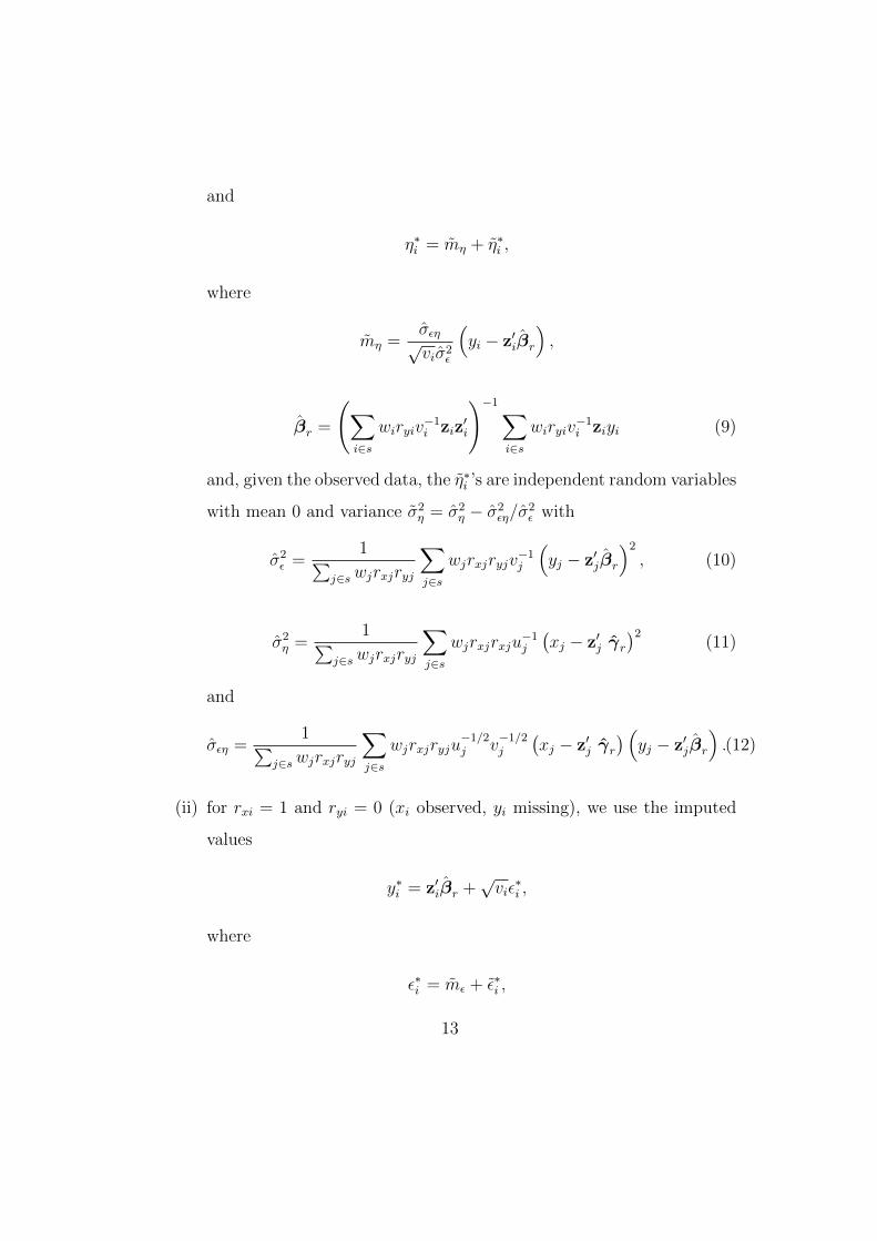
and

η∗i = mη + η∗i ,

where

mη =σεη√viσ2

ε

(yi − z′iβr

),

βr =

(∑i∈s

wiryiv−1i ziz

′i

)−1∑i∈s

wiryiv−1i ziyi (9)

and, given the observed data, the η∗i ’s are independent random variables

with mean 0 and variance σ2η = σ2

η − σ2εη/σ

2ε with

σ2ε =

1∑j∈swjrxjryj

∑j∈s

wjrxjryjv−1j

(yj − z′jβr

)2, (10)

σ2η =

1∑j∈swjrxjryj

∑j∈s

wjrxjrxju−1j

(xj − z′j γr

)2(11)

and

σεη =1∑

j∈swjrxjryj

∑j∈s

wjrxjryju−1/2j v

−1/2j

(xj − z′j γr

) (yj − z′jβr

).(12)

(ii) for rxi = 1 and ryi = 0 (xi observed, yi missing), we use the imputed

values

y∗i = z′iβr +√viε∗i ,

where

ε∗i = mε + ε∗i ,

13

mε =σεη√uiσ2

η

(xi − z′i γr)

and, given the observed data, the ε∗i ’s are independent random variables

with mean 0 and variance σ2ε = σ2

ε − σ2εη/σ

2η.

(iii) For rxi = 0 and ryi = 0 (both xi and yi missing), we use the imputed

values

x∗i = z′i γr +√uiη∗i

y∗i = z′iβr +√viε∗i ,

where (ε∗i , η∗i )’s are independently distributed with mean 0 and covari-

ance matrix

Σ1 =

(σ2ε , σεησεη, σ

2η

)There exist numerous ways for generating the ε∗i ’s and η∗i ’s. Under the

IM approach, Shao and Wang (2002) showed that this joint regression impu-

tation method leads to asymptotically unbiased estimators of coefficients of

correlation, provided the ε∗i ’s and η∗i ’s are independently selected from any

distribution with appropriate mean and variance. They argued that the ran-

dom residuals should be generated from the respondents’ residuals if other

non-linear parameters such as quantiles are of interest. In any case, the

procedures described by Shao and Wang (2002) all suffer from an an extra

variability, called the imputation variance, due to the random selection of the

residuals. As a result, these procedures are not fully efficient, a term coined

by Kim and Fuller (2004).

14

3.2 Balanced imputation procedure

To develop a fully efficient procedure, we first express the total error of ρxyI

as

ρxyI − ρxy = (ρxyπ − ρxy) + (ρxyI − ρxyπ) + (ρxyI − ρxyI) . (13)

The first term on the right hand side of (13) represents the sampling error,

whereas the second and the third terms represent the nonresponse error and

the imputation error, respectively. In order to eliminate the imputation

variance, we suggest selecting the residuals ε∗i and η∗i at random so that the

imputation error, ρxyI − ρxyI , is equal to zero. In other words, we select the

residuals so that the following constraints are satisfied:

tkl,I − tkl,I = 0 (14)

for (k, l) ∈ {(1, 0), (2, 0), (1, 1), (0, 1), (0, 2)}, where tkl,I = EI(tkl,I |x,y, δ, r).

An imputation procedure satisfying (14) has been called a balanced imputa-

tion procedure by Chauvet, Deville and Haziza (2010).

To fix ideas, we first consider the case (k, l) = (1, 0). We have

t10,I =∑i∈s

wixi

=∑i∈s

wirxixi +∑i∈s

wi (1− rxi) ryix∗i +∑i∈s

wi (1− rxi) (1− ryi)x∗i

=∑i∈s

wirxixi +∑i∈s

wi (1− rxi) z′i γr

+∑i∈s

wi (1− rxi) ryi√uiη∗i +

∑i∈s

wi (1− rxi) (1− ryi)√uiη∗i .

15

It follows that t10,I − t10,I = 0 if the balancing equations∑i∈s

wi (1− rxi) ryi√ui (η

∗i − mη) =

∑i∈smr

wi√ui (η

∗i − mη)

= 0 (15)

and ∑i∈s

wi (1− rxi) (1− ryi)√uiη∗i =

∑i∈smm

wi√uiη∗i

= 0 (16)

are satisfied. Similar balancing equations may be derived for any of the

constraints in (14). After some algebra, we obtain that the constraints in (14)

are satisfied if the imputation procedure is such that (i) the four balancing

equations (corresponding to imputation on smr)∑i∈smr

wi√ui (η

∗i − mη) [1, z′i γr, yi] = 0 (17)∑

i∈smr

wiui[η∗2i − (m2

η + σ2η)]

= 0

are satisfied; (ii) the four balancing equations (corresponding to imputation

on srm) ∑i∈srm

wi√vi (ε

∗i − mε)

[1, z′i βr, xi

]= 0 (18)∑

i∈srm

wivi[(ε∗2i − (m2

ε + σ2ε )]

= 0

are satisfied and (iii) the seven balancing equations (corresponding to impu-

16

tation on smm) ∑i∈smm

wi

[z′i γr, z

′i βr

] [√uiη∗i ,√viε∗i

]′= 0∑

i∈smm

wi[ui(η∗2i − σ2

η

), vi(ε∗2i − σ2

ε

)]= 0 (19)∑

i∈smm

wi√uivi [η

∗i ε∗i − σεη] = 0

are satisfied. In other words, we perform the imputations separately on

each of the sub-samples smr, srm and smm. The algorithm for performing

the random selection of residuals while satisfying (17)-(19) is described in

Section 3.3.

3.3 Balanced imputation algorithm

We assume that ε∗i and η∗i are generated from the set of respondent residuals.

We introduce further notation. Let

exj = u−1/2j

(xj − z′j γr

),

eyj = v−1/2j

(yj − z′j βr

)and

(exj, eyj)′ = Σ

−1/22

(xj − z′j γrr, yj − z′j βrr

)′with

βrr =

(∑i∈s

wirxiryiv−1i ziz

′i

)−1∑i∈s

wirxiryiv−1i ziyi,

γrr =

(∑i∈s

wirxiryiu−1i ziz

′i

)−1∑i∈s

wirxiryiu−1i zixi,

17

and

Σ2 =

(σ2ε,rr, σεησεη, σ

2η,rr

),

where

σ2ε,rr =

1∑j∈swjrxjryj

∑j∈s

wjrxjryj

(yj − z′jβrr

)2,

σ2η,rr =

1∑j∈swjrxjryj

∑j∈s

wjrxjryj(xj − z′j γrr

)2.

In order to select the random residuals, we extend the balanced impu-

tation procedure described in Chauvet, Deville and Haziza (2010). It is

presented next:

Step 1: (xi is missing but yi is observed)

Build a nmr × (nrm + nrr) table, where the cell (i, j) is given the prob-

ability of selection φij = wj/∑

l∈swlrxl, and the values

t0ij = wiφij√uiexj [1, z′i γr, yi,

√uiexj]

and

t1ij = (t1ij, . . . , tnmrij )′,

where tkij = φijaki such that aki = 1 if k = i and aki = 0, otherwise,

k = 1 · · ·nmr. A random sample of cells s∗mr is selected with inclusion

probabilities φij and balancing variables t0ij and t1ij. If the cell (i, j) is

selected, then we let η∗i = ση exj.

Step 2: (yi is missing but xi is observed)

Build a nrm× (nmr + nrr) table, where the cell (i, j) is given the prob-

ability of selection φij = wj/∑

l∈swlryl, and the values

t0ij = wiφij√vieyj

[1, z′i βr, xi,

√vieyj

]18

and

t1ij = (t1ij, . . . , tnrmij )′,

where tkij = φijaki, k = 1 · · ·nrm. A random sample of cells s∗rm is

selected with inclusion probabilities φij and balancing variables t0ij and

t1ij. If the cell (i, j) is selected, then we let ε∗i = σε eyj.

Step 3: (both xi and yi are missing)

Build a nmm×nrr table, where the cell (i, j) is given the probability of

selection φij = wj/∑

l∈swjrxlryl, and the values

t0ij = wiφij

[√ui(z

′i γr)exj,

√ui(z

′i βr)exj,

√vi(z

′i γr)eyj,

√vi(z

′i βr)eyj, uie

2xj, vie

2yj,√uiviexj eyj

]and

t1ij = (t1ij, . . . , tnmmij )′,

where tkij = φijaki, k = 1 · · ·nmm. A random sample of cells s∗mm is

selected with inclusion probabilities φij and balancing variables t0ij and

t1ij. If the cell (i, j) is selected, then we let [ε∗i , η∗i ]′ = Σ

1/21 [eyj, exj]

′.

The balancing conditions on variables t1ij ensure that exactly one residual

will be selected for each nonrespondent. In steps 1-3, the balancing con-

ditions on variables t0ij enable us to satisfy the sets of balancing equations

(17)-(19). In this case, the imputation variance is eliminated and the im-

putation procedure is fully efficient. Even if the balancing conditions hold

only approximately, we expect the imputation variance to be significantly

reduced. This is illustrated in Section 5.

19

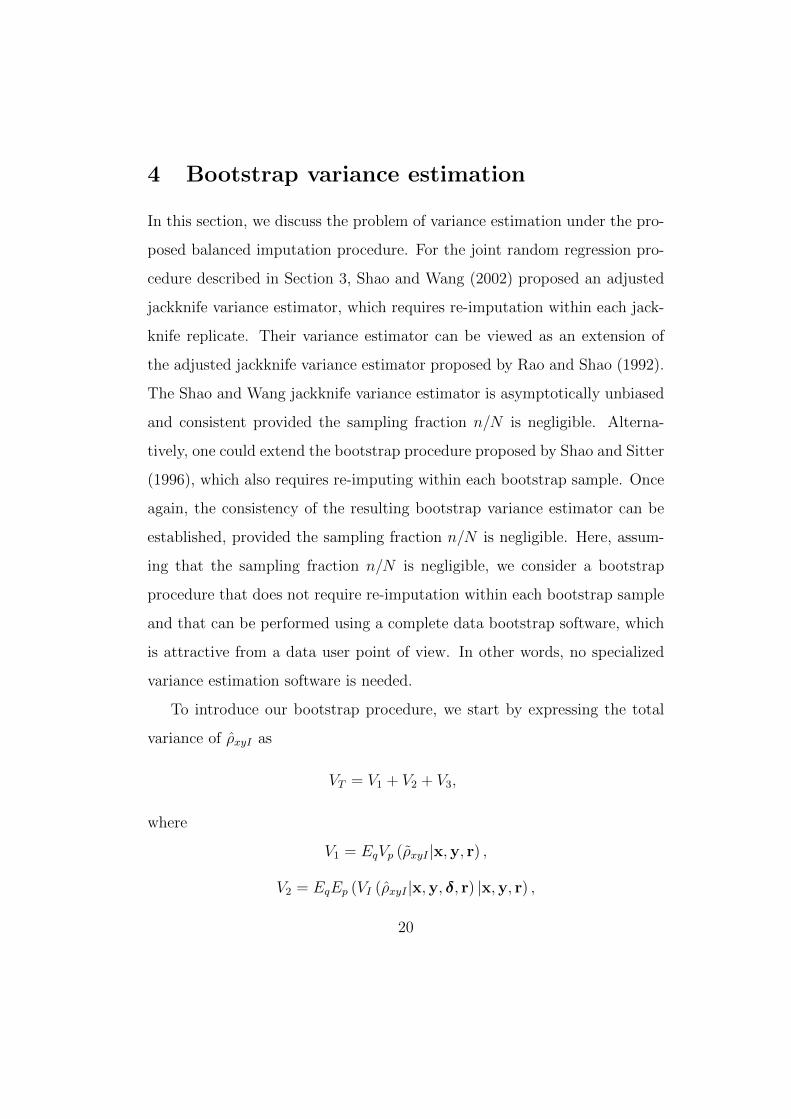
4 Bootstrap variance estimation

In this section, we discuss the problem of variance estimation under the pro-

posed balanced imputation procedure. For the joint random regression pro-

cedure described in Section 3, Shao and Wang (2002) proposed an adjusted

jackknife variance estimator, which requires re-imputation within each jack-

knife replicate. Their variance estimator can be viewed as an extension of

the adjusted jackknife variance estimator proposed by Rao and Shao (1992).

The Shao and Wang jackknife variance estimator is asymptotically unbiased

and consistent provided the sampling fraction n/N is negligible. Alterna-

tively, one could extend the bootstrap procedure proposed by Shao and Sitter

(1996), which also requires re-imputing within each bootstrap sample. Once

again, the consistency of the resulting bootstrap variance estimator can be

established, provided the sampling fraction n/N is negligible. Here, assum-

ing that the sampling fraction n/N is negligible, we consider a bootstrap

procedure that does not require re-imputation within each bootstrap sample

and that can be performed using a complete data bootstrap software, which

is attractive from a data user point of view. In other words, no specialized

variance estimation software is needed.

To introduce our bootstrap procedure, we start by expressing the total

variance of ρxyI as

VT = V1 + V2 + V3,

where

V1 = EqVp (ρxyI |x,y, r) ,

V2 = EqEp (VI (ρxyI |x,y, δ, r) |x,y, r) ,

20

and

V3 = VqEp (ρxyI |x,y, r) ;

see Fay (1991) and Shao and Steel (1999). Note that the term V2 denotes

the imputation variance arising solely from the random selection of residu-

als. In the case of the proposed balanced imputation procedure, the residuals

are randomly selected so that the imputation variance is eliminated. Hence,

the term V2 is (approximately) equal to zero and can be omitted from the

variance calculations. Also, under mild regularity conditions, the contribu-

tion of V3 to the total variance, V3/VT , is of order O(n/N). Thus, when

the sampling fraction n/N is negligible, the contribution of the term V3 to

the total variance is negligible and, as a result, can also be omitted from

the variance calculations. It remains to estimate the term V1 consistently.

To that end, it suffices to estimate Vp (ρxyI |x,y, r) consistently. Noting that

EI (ε∗i |x,y, δ, r) = EI (η∗i |x,y, δ, r) = 0, it follows that ρxyI can be written as

a smooth function of estimated totals since it corresponds to the estimator of

ρxy that we would have obtained under the deterministic version of the Shao-

Wang procedure. The problem of estimating Vp (ρxyI |x,y, r) reduces to the

classical problem of estimating the sampling variance of a smooth function of

estimated totals conditionally given x,y and r. Any complete data variance

estimation method can thus be used (e.g., Taylor linearization, jackknife or

bootstrap). For the proposed balanced imputation procedure, resampling

methods such as the jackknife and the bootstrap are more appealing because

a Taylor linearization procedure would involve very messy calculations. In

this paper, we focus on bootstrap variance estimation.

For simplicity, we consider a special case of the joint random regression

21

imputation procedure described in Section 3.1, which can be called joint

random ratio imputation. It is obtained from (i)-(iii) in Section 3.1 by letting

zi = zi (a scalar) and ui = vi = zi. Assuming that the sample size n is large,

we can approximate ρxyI by

ρxyI.=

t11,I − t10,I t01,I/Nπ(t20,I − (t10,I)2/Nπ

)1/2 (t02,I − (t01,I)2/Nπ

)1/2 .After some algebra, we obtain

t10,I =∑i∈s

wirxixi +∑i∈s

wi(1− rxi)ryi[ziγr +

σεησ2ε

(yi − ziβr

)]+

∑i∈s

wi(1− rxi)(1− ryi) [ziγr] ,

t20,I =∑i∈s

wirxix2i

+∑i∈s

wi(1− rxi)ryi

[uiVI (η∗i |x,y, δ, r) +

(ziγr +

σεησ2ε

(yi − ziβr

))2]

+∑i∈s

wi(1− rxi)(1− ryi)[uiVI (η∗i |x,y, δ, r) + (ziγr)

2]and

t11,I =∑i∈s

wirxiryixiyi

+∑i∈s

wi(1− rxi)ryiyi[ziγr +

σεησ2ε

(yi − ziβr

)]+

∑i∈s

wi(1− ryi)rxixi[ziβr +

σεησ2η

(xi − ziγr)]

+∑i∈s

wi(1− rxi)(1− ryi)[√

uivi CovI (η∗i , ε∗i |x,y, δ, r) + (ziγr)

(ziβr

)],

where γr, βr, σ2ε , σ

2η and σεη are given by (8)-(12), respectively. The terms

t01,I and t02,I may be obtained similarly. Due to the non-independence in the

22

selection of the random residuals for the proposed balanced imputation pro-

cedure, the terms VI (η∗i |x,y, δ, r), VI (η∗i |x,y, δ, r) and CovI (η∗i , ε∗i |x,y, δ, r)

are difficult to compute exactly. One option consists of replacing these terms

by an approximation; see Deville and Tille (2005). Here, we propose to use

a somewhat simpler, conservative approximation: the required terms are re-

placed with the values obtained under the original procedure of Shao and

Wang (2002), where the random residuals are selected independently in each

of the subsamples smr, srm and smm. This leads to the new set of equations

t10,I =∑i∈s

wirxixi +∑i∈s

wi(1− rxi)ryi[ziγr +

σεησ2ε

(yi − ziβr

)]+

∑i∈s

wi(1− rxi)(1− ryi) [ziγr] , (20)

t20,I.=

∑i∈s

wirxix2i

+∑i∈s

wi(1− rxi)ryi

[ui

(σ2η −

σεησ2ε

)+

(ziγr +

σεησ2ε

(yi − ziβr

))2]

+∑i∈s

wi(1− rxi)(1− ryi)[uiσ

2η + (ziγr)

2] (21)

and

t11,I.=

∑i∈s

wirxiryixiyi

+∑i∈s

wi(1− rxi)ryiyi[ziγr +

σεησ2ε

(yi − ziβr

)]+

∑i∈s

wi(1− ryi)rxixi[ziβr +

σεησ2η

(xi − ziγr)]

+∑i∈s

wi(1− rxi)(1− ryi)[√

uiviσεη + (ziγr)(ziβr

)]. (22)

23

As a result, each of the terms tkl,I may be expressed as a smooth function of

estimated totals. We can thus apply any complete data bootstrap procedure

to estimate the term V1. To illustrate the method, we consider the special

case of simple random sampling without replacement. For other sampling de-

signs, any complete data bootstrap procedure leading to consistent variance

estimation can be used. We consider the so-called bootstrap weight proce-

dure proposed by Rao, Wu and Yue (1992), which is popular in practice. It

can be described as follows:

1. Let n′ be the bootstrap sample size, which may be different from n.

2. Draw a simple random sample s∗ of size n′ with replacement from

s. Let m∗i be the number of times unit i is selected in s∗. We have

n′ =∑

i∈sm∗i . For unit i, define the bootstrap weight as

w∗i =

[1 +√C

(nm∗in′− 1

)]wi, for i = 1, · · · , n,

where

C =n′(1− n

N)

n− 1.

Calculate

ρ∗xyI =t∗11,I − t∗10,I t∗01,I/N∗π(

t∗20,I − (t∗10,I)2/N∗π

)1/2 (t∗02,I − (t∗01,I)

2/N∗π

)1/2 ,where N∗π =

∑i∈sw

∗i and t∗10,I , t

∗20,I and t∗11,I are respectively obtained

from (8)-(12) and (20)-(22) by replacing wi with w∗i . The terms t∗01,I

and t∗02,I are obtained similarly.

3. Repeat Step 2 a large number of times, B, to get ρ∗(1)xyI , · · · , ρ

∗(B)xyI .

24

4. Estimate

Vp (ρxyI |x,y, r)

by

VB =1

B − 1

B∑b=1

[ρ∗(b)xyI − ρ

∗(.)xyI

]2, (23)

where ρ∗(.)xyI = 1

B

∑Bb=1 ρ

∗(b)xyI .

5 Simulation study

5.1 Performance of point estimators

We conducted a limited simulation study similar to that of Shao and Wang

(2002) to investigate the performance of the proposed balanced imputation

procedure in terms of bias and relative efficiency. We first generated 3 finite

populations of size N = 4 000, each containing two study variables, x and y,

and one auxiliary variable z. The variable z was first generated independently

from a Gamma distribution with mean 2 and variance 0.1. Then, given the z-

values, bivariate data (xi, yi)’s were generated according to (3), with zi = zi,

ui = vi = zi, and β = γ = 1. The error terms εi and ηi were independently

generated according to

εi = κ χi + νi

and

ηi = κ χi + ςi,

where χi, νi and ςi were independently generated according to a normal

distribution with mean 0 and variance 1, and κ is a parameter whose value

was set to κ = 0.62 for population 1, κ = 0.97 for population 2 and κ = 1.51

25

for population 3. Table 1 shows the population coefficient of correlation

between x and y in each population.

Table 1: Coefficient of correlation for the three generated populations

Population 1 2 3Correlation coefficient ρxy 0.29 0.49 0.70

From each population, we selected 1000 simple random samples without

replacement of size n = 200. Then, in each generated sample, respondents

were generated according to following nonresponse mechanisms:

Pr[rxi = 1|zi] =exp0.1+0.25zi

1 + exp0.1+0.25zi(24)

and

Pr[ryi = 1|zi] =exp0.1+0.25zi

1 + exp0.1+0.25zi(25)

with independent rxi’s and ryi’s. The marginal average of the response prob-

abilities for both x and y was approximately equal to 65% .

In each sample, we computed ρxyI based on (i) marginal random ratio

imputation (MRI), (ii) the Shao and Wang procedure (SW) and (iii) the

proposed balanced random regression imputation (BRI). To measure the bias

of ρxyI , we used the Monte Carlo Percent Relative Bias (RB) given by

RB(ρxyI) =EMC(ρxyI)− ρxy

ρxy× 100, (26)

where EMC(ρxyI) = 11000

∑1000r=1 ρ

(r)xyI and ρ

(r)xyI denotes the estimator ρxyI in

the r-th sample, r = 1, . . . , 1000. To measure of variability of ρxyI , we used

the Monte Carlo Mean Square Error (MSE) given by

MSE(ρxyI) =1

1 000

1000∑r=1

(ρ(r)xyI − ρxy

)2. (27)

26

Let ρMRIxyI , ρSWxyI and ρBRIxyI denote the estimator ρxyI under MRI, SW and

BRI, respectively. In order to compare the relative efficiency of the imputed

estimators, using ρSWxyI as the reference, we used the following measure:

RE =MSEMC(ρ

(.)xyI)

MSEMC(ρ(SW )xyI )

. (28)

Table 2 shows the Monte Carlo Percent Relative Bias (RB) and the RE of

the imputed estimator for each of the three imputation strategies: MRI, SW

and BRI. It is clear that MRI did not preserve the relationship between x and

y for all three populations, as expected. The RB is substantial (more than

50% in all the scenarios) and negative, which clearly illustrates that marginal

imputation attenuates the relationship between variables. Unlike MRI, both

SW and BRI showed a small bias for all three populations, which indicates

that both imputation procedures succeeded in preserving the relationship

between x and y. Turning to the RE, we note that the BRI is more efficient

than SW with a value of RE equal to 0.81 for population 1, 0.79 for population

2 and 0.77 for population 3. Therefore, BRI is significantly more efficient than

SW.

Table 2: Monte-Carlo Relative Bias of the imputed estimator and RE

MRI SW BRIκ = 1 RB(ρxyI) -51.3 -1.6 -0.7

RE 2.25 1 0.81κ = 2 RB(ρxyI) -57.2 -0.3 -0.5

RE 9.45 1 0.79κ = 3 RB(ρxyI) -56.6 -0.3 -0.3

RE 44.73 1 0.77

27

5.2 Performance of the Bootstrap variance estimator

We performed a limited simulation study to assess the performance of the

proposed bootstrap variance estimator in terms of relative bias. We generated

three populations of size N = 10, 000 with two study variables, x and y,

and one auxiliary variable z. We first generated z according to a Gamma

distribution with mean 100 and standard deviation 50. Then, as in Section

5.1, bivariate data (xi, yi)’s were generated so that the population coefficient

of correlation approximately equaled 0.3 for population 1, 0.5 for population

2 and 0.7 for population 3.

From each population, we selected R = 1000 simple random samples

without replacement of size n = 200. Note that the sampling fraction n/N

is equal to 0.02, which can be considered negligible. Then, in each generated

sample, respondents to items x and y were generated independently according

to (24) and (25).

We were interested in estimating the variance of ρxyI under the proposed

balanced random regression imputation (BRI). In each sample (containing

respondents and nonrespondents), we selected B = 2, 000 bootstrap samples

according to the bootstrap weight procedure in Section 4. To measure the

bias of VB (see 23), we used the Monte Carlo percent relative bias given by

RBMC(VB) = 100×EMC

(VB − VMC(ρxyI)

)VMC(ρxyI)

, (29)

where EMC(VB) =∑1000

r=1 V(r)B /1000 with V

(r)B denoting the estimator VB in

the r-th sample and VMC(ρxyI) is a simulation-based approximation of the

true variance, obtained from an independent run of 10, 000 simulations.

Finally, we computed confidence intervals by means of the percentile

28

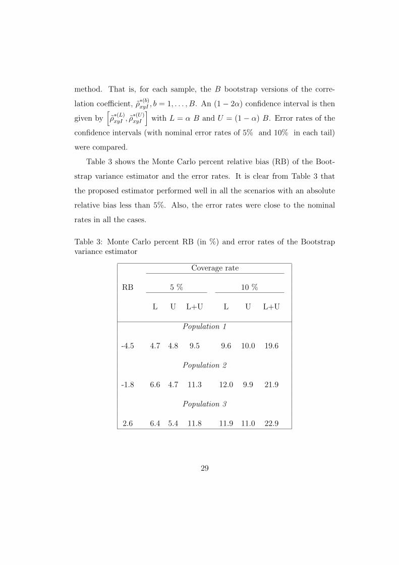
method. That is, for each sample, the B bootstrap versions of the corre-

lation coefficient, ρ∗(b)xyI , b = 1, . . . , B. An (1− 2α) confidence interval is then

given by[ρ∗(L)xyI , ρ

∗(U)xyI

]with L = α B and U = (1− α) B. Error rates of the

confidence intervals (with nominal error rates of 5% and 10% in each tail)

were compared.

Table 3 shows the Monte Carlo percent relative bias (RB) of the Boot-

strap variance estimator and the error rates. It is clear from Table 3 that

the proposed estimator performed well in all the scenarios with an absolute

relative bias less than 5%. Also, the error rates were close to the nominal

rates in all the cases.

Table 3: Monte Carlo percent RB (in %) and error rates of the Bootstrapvariance estimator

Coverage rate

RB 5 % 10 %

L U L+U L U L+U

Population 1

-4.5 4.7 4.8 9.5 9.6 10.0 19.6

Population 2

-1.8 6.6 4.7 11.3 12.0 9.9 21.9

Population 3

2.6 6.4 5.4 11.8 11.9 11.0 22.9

29

6 Concluding Remarks

In this paper, we proposed a fully efficient version of the Shao and Wang

(2002) imputation procedure. Results from a limited simulation study con-

firm the good performance of the proposed method both in terms of relative

bias and relative efficiency. Furthermore, motivated by the reverse framework

of Fay (1991) and Shao and Steel (1999), we proposed a bootstrap variance

estimator, which performed well both in terms of relative bias and coverage

rate of confidence intervals.

References

Chauvet, G., Deville, J.C. and Haziza, D. (2010). On balanced random

imputation in surveys. To appear in Biometrika.

Deville, J.C. (1999). Variance estimation for complex statistics and esti-

mators: linearization and residual techniques. Survey Methodology, 25,

193-203.

Deville, J-C. and Tille, Y. (2005). Variance approximation under balanced

sampling. Journal of Statistical Planning and Inference, 128, 569-591.

Fay, R.E. (1991). A design-based perspective on missing data Variance.

Proceedings of the 1991 Annual Research Conference, US Bureau of the

Census, 429-440.

Haziza, D. (2009). Imputation and inference in the presence of missing data.

In Handbook of Statistics, Volume 29, Sample Surveys: Theory Methods

and Inference, Editors: C.R. Rao and D. Pfeffermann, 215-246.

30

Kim, J.K. and Fuller, W.A. (2004). Fractional hot-deck imputation.

Biometrika, 91, 559-578.

Rao, J. N. K. and Shao, J. (1992). On variance estimation under imputation

for missing data. Biometrika, 79, 811-822.

Rao, J. N. K., Wu, C. F. J. and Yue, K. (1992). Some recent work on

resampling methods for complex surveys. Survey Methodology, 18, 209-

217.

Rubin, D. B. (1976). Inference and missing Data. Biometrika, 63, 581-590.

Santos, R. (1981). Effects of imputation on regression-coefficients. Pro-

ceedings of the Section on Survey Research Methods, American Statistical

Association, 140-145.

Shao, J. and Sitter, R. R. (1996). Bootstrap for imputed survey data. Journal

of the American Statistical Association, 93, 819-831.

Shao, J. and Steel, P. (1999). Variance estimation for survey data with

composite imputation and nonnegligible sampling fractions. Journal of

the American Statistical Association, 94, 254-265.

Shao, J. and Wang, H. (2002). Sample correlation coefficients based on sur-

vey data under regression imputation. Journal of the American Statistical

Association, 97, 544-552.

Skinner, C. J. and Rao, J. N. K. (2002). Jackknife variance for multivariate

statistics under hot deck imputation from common donors. Journal of

Statistical Planning and Inference, 102, 149-167.

31