District-Level Estimates of Fertility and Implied Sex Ratio at ...

SPECIAL ARTICLE

august 18, 2012 vol xlviI no 33 EPW Economic & Political Weekly66

District-Level Estimates of Fertility and Implied Sex Ratio at Birth in India

Sanjay Kumar, K M Sathyanarayana

With an emphasis on decentralised planning in India, the

district has become the primary unit of planning and

monitoring development programmes. The Census of

India is the only source providing useful demographic

information at the district and administrative levels

below it. The findings of this study indicate that India is

undergoing a fertility transition, yet around one-third of

districts have a birth rate of 25 or more. High fertility

districts have shown a faster pace of decline.

Furthermore, around a quarter of the districts are

characterised by a very low implied sex ratio at birth, of

less than 900. Spatial analysis reveals a contiguous

pattern of low ratios in the north-western part of the

country and emerging pockets in Maharashtra and

Gujarat followed by Orissa.

The views expressed in the paper are that of the authors and does not refl ect those of the organisation with which they are affi liated.

Sanjay Kumar ([email protected]) and K M Sathyanarayana ([email protected]) are with the United Nations Population Fund, India.

Appendix Table A1 is placed on the EPW website along with the text of this article.

The Census of India, conducted decennially, provides useful demographic information at the district level and administrative levels below it. The census information

is in general eagerly awaited as there remains dire need of information for facilitating decentralised planning. Even though there are many other important sources such as the Civil Registration System (CRS), Sample Registration System (SRS) and periodic surveys (District-Level Household and Facility Survey and Annual Health Survey) providing demographic in-formation, these sources have their own limitations in terms of coverage, quality as well as the level of disaggregation for which estimates are provided. For instance, CRS provides informa-tion on registered births and deaths, but suffers from coverage and content errors, resulting in gross underestimation of vital indicators. As a result, reliable estimates of important indicators like crude birth rate (CBR) and sex ratio at birth (SRB) are not available at the district level.

While detailed census information for computation of fertility and mortality indicators usually comes after a lag of two years or so after the completion of population enumer-ation phase, the Census of India, since 1991, has been pro-viding quick provisional population estimates by sex, for the overall population, 0-6 year population and over seven years literate population, disaggregated up to the district level. Although the main purpose of providing the 0-6 popu-lation age group is to enable computation of the effective literacy rate, demographers have considered this a vital piece of information and have computed fertility indicators at the sub-national level by reversing the surviving population in this age group.

With a reverse survival technique, the number of births that have occurred during the seven-year period preceding the census can be estimated. The population count in the age category of 0-9 years has generally been found to be reasonably accurate (United Nations 1983). Furthermore, in the Indian context, the proportion of population counted in the 0-6 years age group has also been found to be fairly reliable (Bhat 1996). Bhat has shown the advantages of reverse-surviving using the 0-6 year age group for estimating the fertility rate, as against using the conventional 0-4 and 5-9 years age groups. He concluded that the age interval 0-6 years appeared to gain from digit preference for fi ve and six years of completed age, offsetting the propensity of greater omission in the age interval 0-4 years, besides providing fertility estimates for a more recent period than the age interval of 0-9 years.

SPECIAL ARTICLE

Economic & Political Weekly EPW august 18, 2012 vol xlviI no 33 67

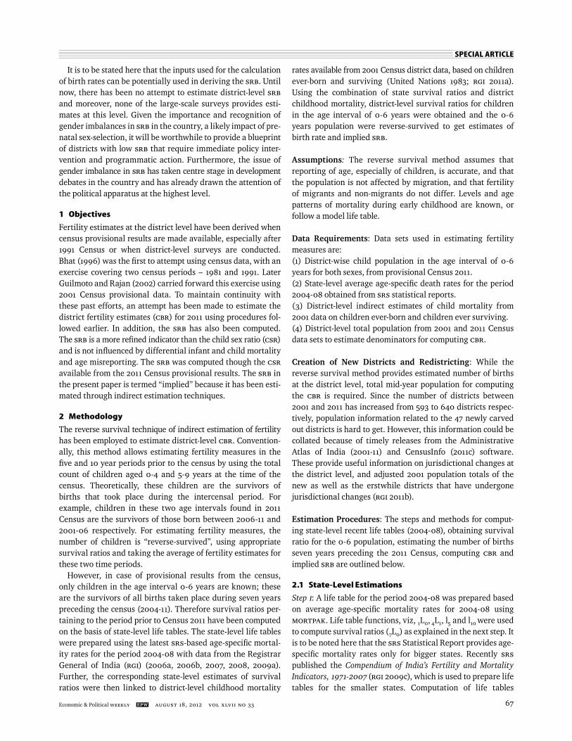
It is to be stated here that the inputs used for the calculation of birth rates can be potentially used in deriving the SRB. Until now, there has been no attempt to estimate district-level SRB and moreover, none of the large-scale surveys provides esti-mates at this level. Given the importance and recognition of gender imbalances in SRB in the country, a likely impact of pre-natal sex-selection, it will be worthwhile to provide a blueprint of districts with low SRB that require immediate policy inter-vention and programmatic action. Furthermore, the issue of gender imbalance in SRB has taken centre stage in development debates in the country and has already drawn the attention of the political apparatus at the highest level.

1 Objectives

Fertility estimates at the district level have been derived when census provisional results are made available, especially after 1991 Census or when district-level surveys are conducted. Bhat (1996) was the fi rst to attempt using census data, with an exercise covering two census periods – 1981 and 1991. Later Guilmoto and Rajan (2002) carried forward this exercise using 2001 Census provisional data. To maintain continuity with these past efforts, an attempt has been made to estimate the district fertility estimates (CBR) for 2011 using procedures fol-lowed earlier. In addition, the SRB has also been computed. The SRB is a more refi ned indicator than the child sex ratio (CSR) and is not infl uenced by differential infant and child mortality and age misreporting. The SRB was computed though the CSR available from the 2011 Census provisional results. The SRB in the present paper is termed “implied” because it has been esti-mated through indirect estimation techniques.

2 Methodology

The reverse survival technique of indirect estimation of fertility has been employed to estimate district-level CBR. Convention-ally, this method allows estimating fertility measures in the fi ve and 10 year periods prior to the census by using the total count of children aged 0-4 and 5-9 years at the time of the census. Theoretically, these children are the survivors of births that took place during the intercensal period. For example, children in these two age intervals found in 2011 Census are the survivors of those born between 2006-11 and 2001-06 respectively. For estimating fertility measures, the number of children is “reverse-survived”, using appropriate survival ratios and taking the average of fertility estimates for these two time periods.

However, in case of provisional results from the census, only children in the age interval 0-6 years are known; these are the survivors of all births taken place during seven years preceding the census (2004-11). Therefore survival ratios per-taining to the period prior to Census 2011 have been computed on the basis of state-level life tables. The state-level life tables were prepared using the latest SRS-based age-specifi c mortal-ity rates for the period 2004-08 with data from the Registrar General of India (RGI) (2006a, 2006b, 2007, 2008, 2009a). Further, the corresponding state-level estimates of survival ratios were then linked to district-level childhood mortality

rates available from 2001 Census district data, based on children ever-born and surviving (United Nations 1983; RGI 2011a). Using the combination of state survival ratios and district childhood mortality, district-level survival ratios for children in the age interval of 0-6 years were obtained and the 0-6 years population were reverse-survived to get estimates of birth rate and implied SRB.

Assumptions: The reverse survival method assumes that reporting of age, especially of children, is accurate, and that the population is not affected by migration, and that fertility of migrants and non-migrants do not differ. Levels and age patterns of mortality during early childhood are known, or follow a model life table.

Data Requirements: Data sets used in estimating fertility measures are:(1) District-wise child population in the age interval of 0-6 years for both sexes, from provisional Census 2011.(2) State-level average age-specifi c death rates for the period 2004-08 obtained from SRS statistical reports. (3) District-level indirect estimates of child mortality from 2001 data on children ever-born and children ever surviving. (4) District-level total population from 2001 and 2011 Census data sets to estimate denominators for computing CBR.

Creation of New Districts and Redistricting: While the reverse survival method provides estimated number of births at the district level, total mid-year population for computing the CBR is required. Since the number of districts between 2001 and 2011 has increased from 593 to 640 districts respec-tively, population information related to the 47 newly carved out districts is hard to get. However, this information could be collated because of timely releases from the Administrative Atlas of India (2001-11) and CensusInfo (2011c) software. These provide useful information on jurisdictional changes at the district level, and adjusted 2001 population totals of the new as well as the erstwhile districts that have undergone jurisdictional changes (RGI 2011b).

Estimation Procedures: The steps and methods for comput-ing state-level recent life tables (2004-08), obtaining survival ratio for the 0-6 population, estimating the number of births seven years preceding the 2011 Census, computing CBR and implied SRB are outlined below.

2.1 State-Level Estimations

Step I: A life table for the period 2004-08 was prepared based on average age-specifi c mortality rates for 2004-08 using MORTPAK. Life table functions, viz, 1L0, 4L1, l5 and l10 were used to compute survival ratios (7L0) as explained in the next step. It is to be noted here that the SRS Statistical Report provides age-specifi c mortality rates only for bigger states. Recently SRS published the Compendium of India’s Fertility and Mortality Indicators, 1971-2007 (RGI 2009c), which is used to prepare life tables for the smaller states. Computation of life tables

SPECIAL ARTICLE


require age-specifi c death rates separately for the 0-1 year and 1-4 years; however, the Compendium provides age-specifi c death rates only for the combined age group of 0-4 years. The bifurcation of age-specifi c rates for smaller states was done by applying the ratio of infant mortality rates to under-fi ve mortality rates. The life table for smaller states pertains to the period 2004-07 as per the latest data availability. Step II: The survival ratio (7L0) for the age group 0-6 years was derived using the following formula:

7L0 = 1L0 + 4L1 + 1.6 l5 + 0.4 l10

Step III: The average annual number of births during the seven years preceding Census 2011 was obtained by the following formula: Population in 0-6 age group × 700000Number of births during seven years = 7L0

Step IV: The mid-year population during 2004-11 was obtained by computing the exponential growth rate of the population during 2001-11 and estimating it at the mid-point of the period 2004-10; this serves as the denominator for computing the CBR.Step V: The CBR per thousand population during the seven years preceding census 2011 was obtained by summing up male and female births and dividing by the mid-year population.Step VI: The implied SRB was computed by dividing the number of female births by male births.

2.2 District-Level Estimates

Calculation of district-level estimates of fertility through the reverse survival technique requires reliable estimates of child-hood mortality for computing survival ratios. An important source for the requisite information on child mortality at the district level is the census itself, as it provides data on ever-born and surviving children to all mothers; through these, indirect estimates of child mortality are obtained using the Brass Technique (United Nations 1983). Ideally, Census 2011 data has to be used but due to the time lag in the release of the required information, Census 2001 estimates of child mortality had to be used.

In using 2001 information, the assumption has been that the pace of decline in district child mortality is in sync with the state-level decline in child mortality. The assumption that all districts experienced the same quantum of decline in child mortality as the state may seem to be a strong one. Yet it has been shown that at moderate levels of mortality, birth rate estimates from the reverse survival procedure are not that sensitive to errors in child mortality estimates. In a typical Indian situation, an error of 10% in the estimate of child mortality results in a less than 2% error in the estimate of the CBR (Bhat 1996). Hence, district survival ratios have been computed accordingly. Step VII: The ratio of district-level child mortality estimates (q5) to the state level (q5) based on the children ever born and children surviving data of the 2001 Census was computed as below: 1000 – District q(5)θ = 1000 – State q(5)

Step VIII: The district-level survival ratio (7LD0) is computed by

7LD0 = 0.27 * (1– θ) * 100000 + θ* 7LS

0

After the district-level survival ratios for both males and females are computed separately, the numbers of male and female births and the mid-year population of the district were obtained as described in Step III to Step V for a given district.

3 Key Findings and Discussions

The fi ndings are presented fi rst at the state level and triangu-lated with other sources of information for validating the results. These include estimation of the reverse survival esti-mates of the CBR and implied SRB. Subsequently, these indicators are presented for each district to enable sharper policy and programmatic focus (see Appendix Table A1, which has been placed on the EPW website).

3.1 Estimates of Reverse Survival CBR

Table 1 provides state-level estimates of CBR derived for the two periods 1994-2000 and 2004-10 using the reverse survival technique, compared with the CBR available from SRS. It can

Table 1: Statewise Estimates of Crude Birth Rate Derived from 2011 Census and other Sources States Reverse Survival Reverse Survival Percentage Average Estimates of Estimates of Decline in CBR, SRS, CBR, 1994-2000* CBR, 2004-10 CBR (1994-2010) 2004-10

India 25.9 21.3 17.8 23.1

Larger States1 Andhra Pradesh 20.4 16.1 21.1 18.6

2 Assam 27.0 23.8 11.9 24.2

3 Bihar 33.4 29.7 11.1 29.3

4 Chhattisgarh 28.6 23.3 18.5 26.4

5 Delhi 23.4 18.7 20.1 18.3

6 Gujarat 22.6 20.1 11.1 23.0

7 Haryana 25.9 21.3 17.8 23.5

8 Jammu & Kashmir 24.5 25.9 -5.7 18.7

9 Jharkhand 29.9 25.8 13.7 26.0

10 Karnataka 20.9 17.8 14.8 20.0

11 Kerala 17.1 14.7 14.0 14.8

12 Madhya Pradesh 30.7 24.4 20.6 28.5

13 Maharashtra 21.7 19.1 12.0 18.2

14 Odisha 23.6 19.6 16.9 21.6

15 Punjab 20.1 16.7 16.9 17.6

16 Rajasthan 32.1 25.6 20.2 27.9

17 Tamil Nadu 17.2 14.9 13.4 16.3

18 Uttar Pradesh 31.4 25.0 20.4 29.6

19 West Bengal 22.5 17.3 23.1 18.0

Smaller States 1 Arunachal Pradesh 29.9 23.1 22.7 21.8

2 Goa 15.9 14.1 11.3 14.1

3 Himachal Pradesh 20.5 17.7 13.7 18.2

4 Manipur 21 19.8 5.7 14.7

5 Meghalaya 33.6 30.1 10.4 24.8

6 Mizoram 27.3 23.5 13.9 18.1

7 Nagaland 24.1 20.8 13.7 16.6

8 Sikkim 23.7 15.1 36.3 18.7

9 Tripura 21.2 18.4 13.2 15.7

10 Uttarakhand 26.1 21.3 18.4 20.3

Correlation coefficient between reverse Survival CBR and SRS CBR 0.772*

* Significant at the 0.01 levelSource: Author’s computations.

SPECIAL ARTICLE


be observed that the CBR, which was 25.9 during the period 1994-2000, had declined to 21.3 births per 1,000 population between 2004 and 2010 resulting in a one-fi fth decline during the reference period. Most of the states in the country, barring Jammu & Kashmir, witnessed declines in the birth rate but the extent of decline varied across the states. The maximum de-cline among the larger states was seen in West Bengal and Andhra Pradesh, while among the smaller states, Sikkim and Arunachal Pradesh showed substantial decline. Among the states with high fertility, Rajasthan, Madhya Pradesh and Uttar Pradesh showed indications of a faster pace of decline whereas the pace of decline in Bihar was slow. Meghalaya was the only state in the country with a birth rate of over 30 and negligible decadal change.

Map 1 depicts a clear pattern of decline in birth rate in the country. States with birth rates lower than 18 have exhibited a clustered type of decline, with all the southern states includ-ing Goa forming one cluster, and West Bengal and Sikkim in the east and Punjab and Himachal Pradesh in the north the second. Interestingly, all the high fertility states in the central region too indicate a contiguous pattern of decline. Further, comparisons of birth rates obtained from reverse survival with SRS estimates reveals that SRS birth rates were higher than reverse survival estimates for the larger states while it was the other way round in case of most of the north-eastern states. One plausible explanation is that the variations in sample-based SRS could partly be due to the standard error or the small sample allocation in smaller states. Nonetheless, the cor-relation between reverse survival and SRS estimates comes out to be 0.772 (signifi cant at the 0.01 level).

3.2 Estimates of Implied SRB

Since the number of births is computed by sex, this procedure allows us to compute the implied sex ratio for the reference period. Such an analysis has been carried out and presented in Table 2. It is to be mentioned here that the Indian defi nition

Map 1: Reversed Survival Estimates of CBR (1994-2000 and 2004-10)

< 18

18 - 20.9

21 - 24.9

25 - 29.9

> 30

Rajasthan

Mizoram

Manipur

Nagaland

Arunachal Pradesh Sikkim

Meghalaya

Uttar Pradesh Assam

NCT of Delhi Haryana

Uttarakhand Chandigarh

Punjab Himachal Pradesh

Jammu & Kashmir

Bihar

Pondicherry Tamil Nadu

Kerala Lakshadweep

Goa Karnataka

Tripura

Maharashtra

Andaman & Nicobar Islands

Gujarat Madhya Pradesh

Chhattisgarh Orissa

Jharkhand West Bengal

Andhra Pradesh

Rajasthan

Mizoram

Manipur

Nagaland

Arunachal Pradesh Sikkim

Meghalaya

Uttar Pradesh Assam


Uttarakhand Chandigarh Punjab

Himachal Pradesh

Jammu & Kashmir

Bihar


Kerala Lakshadweep

Goa Karnataka

Tripura

Maharashtra


Gujarat Madhya Pradesh

Chhattisgarh Orissa


Andhra Pradesh

Table 2: Statewise Child Sex Ratio (0-6 Age Population), Implied Sex Ratio at Birth and Sex Ratio at Birth from SRS State CSR (0-6 age Implied SRB Difference SRS SRB, Group), 2011 (Females to Males) (Implied SRB-CSR) 2007-09

India 914 919 5 906

Larger States

1 Andhra Pradesh 943 942 -1 919

2 Assam 957 952 -5 931

3 Bihar 933 941 8 917

4 Chhattisgarh 964 963 -1 980

5 Delhi 866 864 -2 882

6 Gujarat 886 891 5 904

7 Haryana 830 842 12 849

8 Jammu & Kashmir 859 870 11 870

9 Jharkhand 943 953 10 921

10 Karnataka 943 944 1 944

11 Kerala 943 959 16 968

12 Madhya Pradesh 912 917 5 926

13 Maharashtra 883 902 19 896

14 Odisha 934 936 2 941

15 Punjab 846 854 8 836

16 Rajasthan 883 889 6 875

17 Tamil Nadu 946 946 0 929

18 Uttar Pradesh 899 911 12 874

19 West Bengal 950 947 -3 944

Smaller States

1 Arunachal Pradesh 960 961 1 --

2 Goa 920 920 0

3 Himachal Pradesh 906 916 10 944

4 Manipur 934 934 0 --

5 Meghalaya 970 967 -3 --

6 Mizoram 971 972 1 --

7 Nagaland 944 945 1 --

8 Sikkim 944 947 3 --

9 Tripura 953 954 1 --

10 Uttarakhand 886 890 4 --

Correlation Coefficient between CSR and SRB 0.987* *Significant at the 0.01 level.Source: Author’s computations.

SPECIAL ARTICLE


of implied SRB, that is ratio of female to male births has been used, while internationally, the defi nition is ratio of males to female births.

For India as a whole, the implied SRB is estimated to be 919 females per 1,000 males, which is higher than the three-year average SRS SRB estimate (906) for the period 2007-09. It is to be reiterated that the estimates of SRB from the SRS are based on a sample and subject to a large confi dence interval. The upper limit of the SRS SRB is estimated to be 911 while the lower limit is 901.1

Likewise variation existed at the state level; 13 out of 29 states had a higher implied SRB than the SRS SRB. The extent of variation in the confi dence interval was enormous and ranged from 33 points (between lower and upper limits of SRB) in Bi-har, to 58 points in Punjab. But on an average, the confi dence interval ranged between 45 and 57 points in the majority of states.

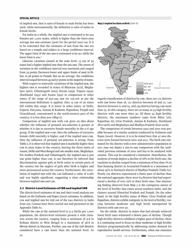
With respect to statewide variations of the implied SRB, the highest SRB is recorded in states of Mizoram (972), Megha-laya (967), Chhattisgarh (963), Kerala (959), Tripura (954), Jharkhand (953) and Assam (952) in comparison to other states. If the range of 952-943 SRB (or 105-106 as per the international defi nition) is applied, then 13 out of 29 states fall within this range. It is lower in other states: in Delhi, Gujarat, Haryana, Jammu & Kashmir, Rajasthan, Punjab and Uttarakhand, concentrated in the north-western part of the country, it is less than 900 (Map 2).

Comparison of implied SRB with CSR gives an idea about whether the infl uence of prenatal sex-selection is greater or whether it is due to excessive female mortality in the 0-6 age group. If the implied SRB>CSR, then the infl uence of excessive female child mortality is higher, and if the implied SRB<CSR, then the infl uence of prenatal sex-selection is strong. From Table 2, it is observed that implied SRB is markedly higher than CSR in most states in the country, barring the three states of Assam, Delhi and West Bengal and one smaller state, Meghalaya. For Andhra Pradesh and Chhattisgarh, the implied SRB is just one point higher than CSR. It can therefore be inferred that discrimination against girls at birth exists in certain parts of the country but the neglect of girls after birth is higher and more pronounced across the country. Furthermore, the corre-lation of implied SRB with the CSR indicated a value of 0.987 and was highly signifi cant, suggesting a close relationship between implied SBR and CSR.

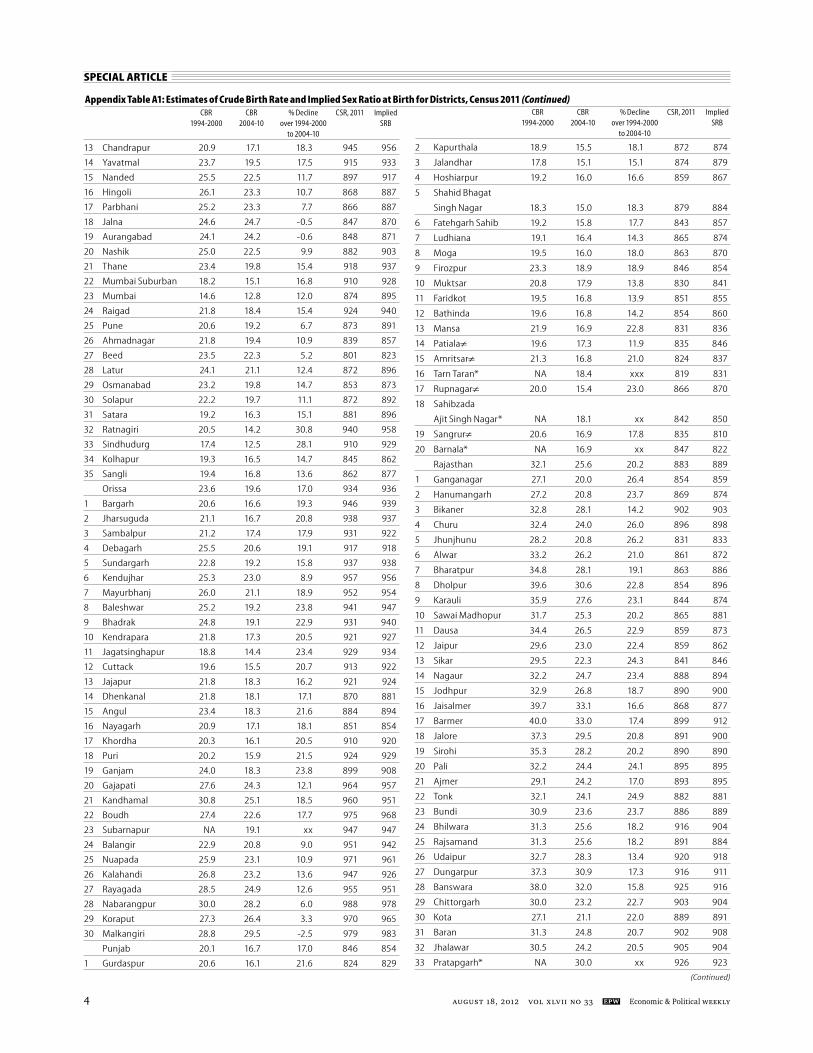
3.3 District-Level Estimates of CBR and Implied SRB

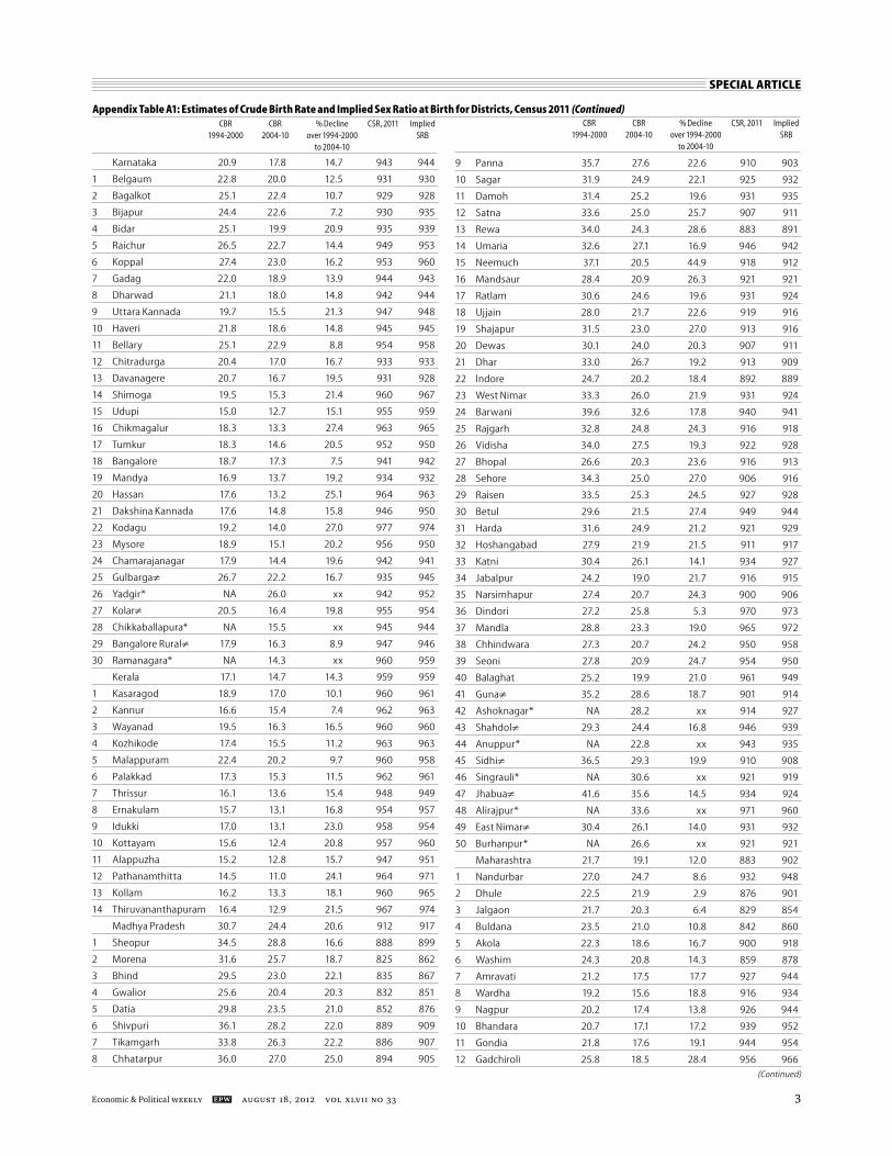
The district-level estimates of CBR and their trend analysis are based on the Guilmoto and Rajan (2002) estimates. In addition, CSR and implied SRB for 628 out of the 640 districts in India from 2011 Census have been carried out and presented in the Appendix Table A1.

While the CBR at the national level is 21.3 births per 1,000 population, the district-level estimates present a wide varia-tion across the country, ranging from a minimum of 9.8 in Kolkata district in West Bengal to a maximum of 38.8 in Mewat district in Haryana. Further, 299 out of the 628 districts considered have a CBR lower than the national level. As

regards classifi cation of districts by CBR, there are 172 districts with CBR lower than 18, 121 districts between 18 and 21; 140 districts between 21 and 25, and 195 districts having CBR more than 25. In this category, there are as many as 53 high fertility districts with CBR more than 30. Of these 53 high fertility districts, the maximum numbers came from Bihar (16), Rajasthan (6), Uttar Pradesh, Jammu & Kashmir, Jharkhand (fi ve each) and Meghalaya and Madhya Pradesh (four each).

The comparison of trends between 1994 and 2010 was pos-sible because of a similar analysis conducted by Guilmoto and Rajan (2002). However, it is to be stated here that 47 new dis-tricts were formed between 2001 and 2011. The birth rate esti-mated for the district with a new administrative population in 2011 may not depict a one-to-one comparison with the undi-vided previous estimate of 2001 and has to be analysed with caution. This can be considered a limitation. Nonetheless, the analysis of trends depicts a decline of 18% in the birth rate; the variation in decline ranged from a minimum of less than 1% in East Kameng district in Arunachal Pradesh to a maximum of about 45% in Neemuch district of Madhya Pradesh (Table A1). Nearly 274 districts experienced a faster pace of decline than the national aggregate; there were 63 districts that had experi-enced a decline of over 25% in their birth rates. One interest-ing fi nding observed from Map 3 is the contiguous nature of the level of fertility that exists across southern India, and the clusters around Himachal Pradesh and Punjab. On the other hand, in the high fertility states of Bihar, Uttar Pradesh and Rajasthan, districts exhibit contiguity in the level of fertility, var-ying between moderate and high levels interspersed by districts with CBR over 30.

On the whole, districts in states that had already achieved lower birth rates witnessed a slower pace of decline. Though high fertility districts exhibited a higher pace of decline, there is a continuing need to focus on these moderate or high fertility districts programmatically by addressing unmet demand for reproductive health services. Furthermore, when one examines

Map 2: Implied Sex Ratio at Birth (2004-10)

Mizoram

Manipur

Nagaland

Arunachal Pradesh

Sikkim

Meghalaya

Assam

Uttarakhand Chandigarh Punjab

Himachal Pradesh

Jammu & Kashmir

Bihar


Kerala

Lakshadweep

Goa Karnataka

Tripura

Maharashtra


Gujarat

Chhattisgarh Orissa


Andhra Pradesh

Rajasthan

Uttar Pradesh


Madhya Pradesh

950 & above

900 - 949

850 - 899

< 850

SPECIAL ARTICLE


the results of undivided districts in Jammu & Kashmir, a clear increase in birth rate is observed. It is diffi cult to conclusively comment on data quality, yet the impression one gets is that the data is suspect and needs further investigation.

The analysis of district-level estimates of the implied SRB indicates substantial variation across the country with the lowest of 783 to the highest of 1,060, with the national average being 919 girls per 1,000 boys (Table A1 in the Appendix). About a quarter of the districts in India (161) are characterised by very low implied SRB (lower than 900), with four districts – Jhajjar (783), Mahendragarh (789), Rewari (788) in Haryana and Samba (794) in Jammu & Kashmir – at less than 800. Fur-ther, there are 30 districts in the range of 800-849, mainly consisting of districts from Haryana (9), Punjab (8), Jammu & Kashmir (4) and Rajasthan (2). The next category included 127 districts with implied SRBs of 850-899. Districts in the states of Uttar Pradesh (21), Rajasthan (19), Maharashtra (16), Punjab (10) and Gujarat (10) accounted for more than half the districts in this category. Bordering states such as Haryana, Jammu & Kashmir, Himachal Pradesh, Uttarakhand and Madhya Pradesh also exhibited adverse ratios. Spatial analysis reveals a contiguous pattern in the north-western part of the country and emerging pockets in Maharashtra and Gujarat followed by Orissa. On the other hand, there are 279 and 188 districts in the 900-949 and 950 and above categories respectively. Evidently, a sizeable number of districts in India experience a low SRB, as seen from this analysis of the implied SRB estimated from the provisional fi gures of the child population from Census 2011.

However, if one were to juxtapose and draw inferences from the declining CSR trends, one can say with conviction that the problem of declining SRB and CSR that had remained an urban phenomenon has now percolated to rural and tribal districts with state-border districts being the most affected, depicting contiguity in spatial distribution. In addition to this observation, it appears that a centrifugal force within the state is operating

wherein districts bordering the lowest implied SRB also have lower implied SRB. This pattern appears to be spreading out (Map 4). This observation is typical in the states of Maharashtra, Punjab and Haryana. Trend analyses would have depicted this better but previous work on indirect fertility estimation from census data by Bhat and Guilmoto et al have not dealt with this important aspect. Therefore, it is diffi cult to analyse trends and the patterns of change. This can be considered a limita-tion of the present paper.

4 Way Forward

Analysis of provisional census data has clearly indicated that district fertility in the country has come down substantially in the past one decade. At the same time, it has also brought out the extent of variation across districts within and between states in the country. Further, it has facilitated the classifi cation of districts by their present level of fertility and the decadal pace of decline. Likewise, implied SRB and its comparison with CSR has enabled an overall picture of prenatal sex-selection and post-birth discrimination in districts of the country.

Programmatically, information related to vital rates, age-specifi c fertility and mortality rates, and SRB are needed continuously not only for prioritising action and evolving area-specifi c plans but also for tracking progress in these indicators. Despite the implementation of decentralisation in the country for nearly three decades, it is hard to get direct

NCTDelhi

EstimatesofCBRBELOW18.018.0-20.921.0-24.925.0-29.930.0ANDABOVE

Map 3: District-Level Estimates of CBR (2004-10) Map 4: District-Level Estimates of Implied SRB (2004-10)

NCTDelhi

p p ,

Estimatesof ImpliedSRBBELOW850850-899900-949950 ANDABOVE

Estimates of implied SRB Below 850 850-899 900-949 950 and above

Estimates of CBR Below 18.0 18.0-20.9 21.0-24.9 25.0-29.9 30.0 and above

available at

Ganapathy Agencies3/4, 2 Link Street

Jaffarkhanpet, Ragavan ColonyChennai 600 083, Tamil Nadu

Ph: 24747538

SPECIAL ARTICLE


estimates at the district level in the country. One has to rely on decennial information from the census and special sample surveys for information, that too employing indirect tech-niques of estimation. Indirect estimation involves making a set of assumptions; there is therefore a need to improve administrative data systems so that quality data is available on a regular and continuous basis.

For this to happen, the focus has to be on improving CRS in the country. Presently, about 12 states and four union territories

References

Bhat, P N Mari (1996): “Contours of Fertility Decline in India: A District Level Study Based on the 1991 Census” in K Srinivasan (ed.), Population Policy and Reproductive Health (New Delhi: Hindustan Publishing Corporation), 96-179.

Guilmoto, C Z and S Irudaya Rajan (2002): “District Level Estimates of Fertility from India’s 2001 Census”, Economic & Political Weekly, 37(7): 665-72.

RGI (2006a): Sample Registration System Statisti-cal Report 2004, Report No 1 of 2006, Offi ce of the Registrar General, New Delhi.

– (2006b): Sample Registration System Statistical Report 2005, Report No 2 of 2006, Offi ce of

the Registrar General, New Delhi. – (2007): Sample Registration System Statistical

Report 2006, Report No 4 of 2007, Offi ce of the Registrar General, New Delhi.

– (2008): Sample Registration System Statistical Report 2007, Report No 2 of 2008, Offi ce of the Registrar General, New Delhi.

– (2009a): Sample Registration System Statistical Report 2008, Report No 1 of 2009, Offi ce of the Registrar General, New Delhi.

– (2009b): Vital Statistics of India Based on the Civil Registration System, Special Report 2002-2005, Offi ce of the Registrar General, New Delhi.

– (2009c): Compendium of India’s Fertility and Mortality Indicators 1971-2007 based on the

Sample Registration System (SRS), Offi ce of the Registrar General, New Delhi.

– (2011a): “Provisional Population Totals”, Paper 1 of 2011, Series 1, Offi ce of the Registrar Gen-eral, New Delhi.

– (2011b): “Administrative Atlas of India”, Census of India, 2011, Offi ce of the Registrar General, New Delhi.

– (2011c): “CensusInfo India Dashboard”. Accessed on 5 September 2011: http://www.censusindia.gov.in/2011-common/census_info.html

United Nations (1983): “Manual X – Indirect Techni-ques for Demographic Estimation”, Population Studies No 81, Department of International Economic and Social Affairs, United Nations, New York.

have been reporting over 90% registration of births in 2005 (RGI 2009b). Efforts to estimate vital rates and SRB at the district level will have to be initiated in these states and validated through SRS and other surveys at the state level. At the same time, concrete efforts are needed to strengthen CRS in states where the reporting is poor. With National Population Register updation on the anvil, it becomes imperative and necessary to set right the basic data systems at disaggregated levels.

EPW Research Foundation (A UNIT OF SAMEEKSHA TRUST)

www.epwrf.in www.epwrfi ts.in India Time SeriesThe EPWRF has further progressed with its online database service christened as ‘India Time Series’, www.epwrfi ts.in. The project introduced a few months ago envisaged dissemination of data in thirteen modules displaying time series on a wide range of macro-economic and fi nancial sector variables in a manner convenient for research and analytical work. This is targeted to benefi t particularly students, research scholars, professionals and the academic community, both in India and abroad. This online service is a part of the project funded by the University Grants Commission (UGC) and executed by the Tata Institute of Social Sciences (TISS), Mumbai and the Economic and Political Weekly (EPW). Time series data set has been structured under various modules.

Modules released so far Following modules will be added soon1) Financial Markets 1) National Accounts Statistics2) Banking Statistics (Basic Statistical Returns) 2) Annual Survey of Industries3) Domestic Product of States of India (SDP) 3) External Sector 4) Agricultural Statistics 4) Finances of State Governments5) Price Indices 6) Power Sector 7) Finances of Government of India 8) Combined Government Finances 9) Industrial Production Series Key Online Database Features● Disseminating data in the time series format.● Interactive online access to time series data updated periodically.● Select data series as per requirement and download at ease.● Instantly compare, plot and analyze different data in relation to each other.● Export to Excel for time series analysis and econometric work.● Save time and energy in data compilation.● Get help needed from our team.

The demo version can be accessed by free registration. The existing members already registered with us and accessing member services at www.epwrf.in will not require fresh registration. To gain full access, the subscription rates are available on our website. For any further details or clarifi cations, please contact:

The Director, EPW Research Foundation, C-212, Akurli Industrial Estate, Akurli Road, Kandivli (East), Mumbai - 400 101.(Phone: +91-22-2885 4995/4996) or mail to: [email protected]

SPECIAL ARTICLE


CBR CBR % Decline CSR, 2011 Implied 1994-2000 2004-10 over 1994-2000 SRB to 2004-10

India 25.9 21.3 17.9 914 919

Andhra Pradesh 20.4 16.1 21.0 943 942

1 Adilabad 23.5 17.1 27.4 942 935

2 Nizamabad 21.9 16.3 25.5 946 945

3 Karimnagar 19.9 13.0 34.7 937 935

4 Medak 23.3 18.2 22.0 954 952

5 Hyderabad 18.6 15.9 14.3 938 947

6 Rangareddy 22.5 19.4 13.8 947 949

7 Mahbubnagar 24.8 20.4 17.9 932 932

8 Nalgonda 21.7 16.0 26.5 921 920

9 Warangal 21.7 14.3 34.0 912 911

10 Khammam 21.0 15.0 28.7 958 957

11 Srikakulam 20.6 15.6 24.4 953 947

12 Vizianagaram 20.7 15.9 23.0 955 945

13 Visakhapatnam 19.6 16.0 18.3 961 960

14 East Godavari 18.6 14.7 21.1 969 965

15 West Godavari 18.0 14.1 21.7 970 964

16 Krishna 18.0 13.9 22.9 953 949

17 Guntur 17.7 14.8 16.4 948 946

18 Prakasam 19.2 16.7 13.3 932 933

19 Sri Potti Sriramulu Nellore 18.5 15.2 17.9 945 940

20 YSR 19.8 17.1 13.8 919 916

21 Kurnool 24.5 19.1 22.2 937 941

22 Anantapur 20.6 16.9 18.1 927 930

23 Chittoor 19.6 16.0 18.4 931 928

Assam 27.0 23.8 11.8 957 952

1 Kokrajhar 29.3 23.6 19.4 951 951

2 Dhubri 35.2 32.2 8.5 965 956

3 Goalpara 32.0 28.0 12.6 954 945

4 Barpeta 30.8 27.9 9.5 955 950

5 Morigaon 31.8 28.1 11.6 950 944

6 Nagaon 29.9 26.5 11.2 958 955

7 Sonitpur 25.6 22.8 11.0 958 952

8 Lakhimpur 27.4 23.6 13.9 958 954

9 Dhemaji 27.7 23.7 14.5 945 942

10 Tinsukia 25.1 21.0 16.4 971 969

11 Dibrugarh 22.0 18.1 17.7 957 963

12 Sivasagar 21.6 18.5 14.6 957 951

13 Jorhat 19.4 16.8 13.2 963 963

14 Golaghat 23.3 19.2 17.5 961 958

15 Karbi Anglong 29.6 31.8 -7.6 916 916

16 Dima Hasao 27.7 24.0 13.5 956 956

17 Cachar 25.3 23.8 6.1 955 948

18 Karimganj 29.0 28.3 2.3 958 952

19 Hailakandi 30.2 27.9 7.5 948 946

20 Bongaigaon 29.4 26.0 11.4 965 958

21 Chirang* NA 23.7 xx 958 954

22 Kamrup 22.1 20.7 6.5 962 960

23 Kamrup Metropolitan* NA 15.5 xx 994 992

24 Nalbari 23.0 18.9 18.0 963 961

25 Baksa* NA 19.8 xx 962 960

26 Darrang 29.1 28.1 3.3 941 934

27 Udalguri* NA 21.5 xx 965 958

Bihar 33.4 29.7 11.2 933 941

1 Paschim Champaran 35.7 32.0 10.3 950 956

2 Purba Champaran 34.8 33.0 5.3 923 935

Appendix Table A1: Estimates of Crude Birth Rate and Implied Sex Ratio at Birth for Districts, Census 2011

3 Sheohar 35.8 32.7 8.7 925 950

4 Sitamarhi 36.3 32.1 11.6 932 956

5 Madhubani 33.3 28.6 14.1 931 943

6 Supaul 36.2 31.6 12.6 942 950

7 Araria 36.2 34.9 3.7 954 948

8 Kishanganj 39.0 35.3 9.6 966 963

9 Purnia 37.6 33.3 11.4 953 956

10 Katihar 38.2 33.4 12.7 956 962

11 Madhepura 36.7 33.3 9.3 923 928

12 Saharsa 35.5 32.6 8.2 928 938

13 Darbhanga 33.1 29.4 11.3 928 946

14 Muzaffarpur 32.7 29.2 10.7 917 928

15 Gopalganj 31.9 27.4 14.0 945 946

16 Siwan 32.9 25.8 21.6 934 928

17 Saran 32.6 26.8 17.8 922 924

18 Vaishali 31.9 28.2 11.7 894 904

19 Samastipur 34.8 30.6 12.2 941 954

20 Begusarai 34.0 29.9 12.1 911 924

21 Khagaria 35.7 34.9 2.3 912 925

22 Bhagalpur 31.9 28.9 9.6 934 939

23 Banka 33.8 29.5 12.9 939 950

24 Munger 29.0 26.0 10.4 925 933

25 Lakhisarai 33.8 30.2 10.6 915 927

26 Sekhpura 34.3 30.6 10.7 940 954

27 Nalanda 31.2 28.6 8.4 929 938

28 Patna 28.4 25.4 10.6 899 909

29 Bhojpur 30.1 26.3 12.7 915 926

30 Buxar 31.7 27.4 13.7 925 937

31 Kaimur 34.4 30.6 11.1 939 952

32 Rohtas 32.1 26.8 16.4 925 932

33 Jehanabad 32.0 28.4 11.3 918 928

34 Aurangabad 32.3 29.4 9.0 945 952

35 Gaya 33.2 29.0 12.7 959 962

36 Nawada 33.3 26.9 19.3 985 994

37 Jamui 32.8 29.6 9.7 956 965

38 Arwal* NA 28.9 xx 941 951

Chhattisgarh 28.6 23.3 18.6 964 963

1 Koriya 27.4 22.8 16.6 968 970

2 Surguja 31.5 25.7 18.6 955 957

3 Jashpur 27.0 23.2 14.1 974 979

4 Raigarh 26.3 20.8 20.9 943 945

5 Korba 28.0 23.0 18.0 964 965

6 Janjgir-Champa 28.0 22.1 21.2 945 945

7 Bilaspur 28.3 25.9 8.5 957 956

8 Kabeerdham NA 30.7 xx 973 967

9 Rajnandgaon 28.1 22.6 19.6 976 971

10 Durg 25.1 20.3 19.1 958 956

11 Raipur 28.4 24.0 15.3 965 963

12 Mahasamund 25.4 20.8 18.1 960 963

13 Dhamtari 27.5 20.2 26.6 969 971

14 Uttar Bastar Kanker 27.0 21.1 21.9 975 971

15 Bastar 29.3 24.8 15.2 991 988

16 Narayanpur* NA 27.0 xx 975 973

17 Dakshin Bastar Dantewada 30.2 23.9 20.7 1,005 1,013

18 Bijapur* NA 25.9 xx 978 986


(Continued)

SPECIAL ARTICLE


NCT of Delhi 23.4 18.7 19.9 866 864

1 North West 25.2 19.7 21.9 863 860

2 North 18.8 17.6 6.4 872 865

3 North East 28.1 21.5 23.4 875 874

4 East 22.6 17.5 22.7 870 868

5 New Delhi 17.1 11.5 32.7 884 874

6 Central 17.2 14.9 13.6 902 896

7 West 21.3 17.7 17.1 867 864

8 South West 24.0 18.7 22.2 836 833

9 South 24.2 18.9 22.1 878 874

Gujarat 22.6 20.1 10.8 886 891

1 Kachchh NA 25.1 xx 913 919

2 Banaskantha 31.3 26.7 14.7 890 900

3 Patan 26.1 22.2 15.1 884 900

4 Mahesana 22.4 17.7 20.8 845 854

5 Sabarkantha 25.1 22.5 10.2 899 901

6 Gandhinagar 22.1 18.5 16.1 847 862

7 Ahmedabad 20.5 18.2 11.3 859 865

8 Surendranagar 27.6 21.6 21.8 889 898

9 Rajkot 16.9 18.0 -6.3 854 857

10 Jamnagar 21.7 18.6 14.3 898 903

11 Porbandar 21.8 16.8 23.0 894 895

12 Junagadh 23.1 17.3 24.9 904 903

13 Amreli 21.1 17.3 18.1 879 884

14 Bhavnagar 25.3 20.3 19.6 885 889

15 Anand 21.7 18.8 13.2 877 884

16 Kheda 23.1 19.6 15.3 887 896

17 Panchmahals 27.7 23.9 13.8 923 924

18 Dohad 34.2 32.6 4.7 937 943

19 Vadodara 21.3 18.2 14.5 894 901

20 Narmada 24.6 20.6 16.3 937 936

21 Bharuch 22.3 17.5 21.7 914 918

22 The Dangs 32.8 28.4 13.3 963 968

23 Navsari 17.9 15.0 16.0 921 916

24 Valsad 22.7 19.4 14.4 926 924

25 Surat 23.2 19.8 14.8 836 838

26 Tapi* NA 16.3 xx 944 946

Haryana 25.9 21.3 18.0 830 842

1 Panchkula 24.1 18.8 22.2 850 865

2 Ambala 20.9 17.1 18.3 807 821

3 Yamunanagar 22.7 19.0 16.1 825 837

4 Kurukshetra 23.0 19.3 16.0 817 817

5 Kaithal 25.1 20.6 18.1 821 838

6 Karnal 24.0 21.0 12.4 820 836

7 Panipat 27.5 22.6 17.7 833 844

8 Sonipat 24.4 20.4 16.3 790 800

9 Jind 26.0 20.0 23.2 835 850

10 Fatehabad 26.3 20.7 21.3 845 855

11 Sirsa 24.7 19.1 22.8 852 862

12 Hisar 25.3 19.3 23.6 849 863

13 Bhiwani 25.5 20.3 20.5 831 839

14 Rohtak 23.5 18.8 20.0 807 819

15 Jhajjar 24.3 19.1 21.6 774 783

16 Mahendragarh 25.5 19.1 25.0 778 789

17 Rewari 25.0 20.2 19.2 784 788

18 Gurgaon 35.2 24.5 30.3 826 842

19 Mewat* NA 38.8 xx 903 921

20 Faridabad 29.9 22.2 25.7 842 861

21 Palwal* NA 27.3 xx 862 881

Jammu & Kashmir 24.5 25.9 -5.6 859 870

1 Kupwara 30.4 38.1 -25.2 854 862

2 Budgam 25.8 33.1 -28.1 832 843

3 Leh(Ladakh) 10.6 13.4 -26.2 944 958

4 Kargil 26.7 25.6 4.2 978 965

5 Punch 30.3 29.3 3.3 895 900

6 Rajouri 28.0 31.2 -11.5 837 850

7 Kathua 24.9 20.6 17.2 836 844

8 Baramulla 26.4 25.9 2.0 866 882

9 Bandipore* NA 25.9 xx 893 909

10 Srinagar 17.5 19.7 -12.8 869 888

11 Ganderbal* NA 28.3 xx 863 883

12 Pulwama 20.8 27.5 -32.4 836 846

13 Shupiyan* NA 24.1 xx 883 893

14 Anantnag 25.0 32.4 -29.6 831 853

15 Kulgam* NA 25.7 xx 882 905

16 Doda 29.1 28.3 2.7 932 942

17 Ramban* NA 31.9 xx 931 939

18 Kishtwar* NA 27.1 xx 922 931

19 Udhampur 27.7 23.9 13.7 887 893

20 Reasi* NA 29.0 xx 921 928

21 Jammu 21.3 16.1 24.3 795 803

22 Samba* NA 18.7 xx 787 794

Jharkhand 29.9 25.8 13.7 943 953

1 Garhwa 37.7 29.9 20.6 958 974

2 Chatra 34.1 30.5 10.4 963 981

3 Kodarma 33.1 29.6 10.4 944 950

4 Giridih 35.8 30.2 15.7 934 945

5 Deoghar 33.2 28.7 13.5 939 958

6 Godda 31.5 29.5 6.3 953 974

7 Sahibganj 35.5 31.1 12.3 955 972

8 Pakur 35.0 32.6 6.9 965 976

9 Dhanbad 24.4 21.0 13.9 917 923

10 Bokaro 25.8 21.4 17.2 912 923

11 Lohardaga 32.9 27.3 17.0 961 969

12 Purbi Singhbhum 22.1 19.6 11.2 922 923

13 Palamu 34.7 27.5 20.6 947 965

14 Latehar* NA 31.1 xx 964 982

15 Hazaribagh 30.0 25.7 14.4 924 929

16 Ramgarh* NA 21.6 xx 926 931

17 Dumka 28.6 25.7 10.1 957 969

18 Jamtara* NA 26.0 xx 948 960

19 Ranchi 26.4 21.5 18.5 937 942

20 Khunti* NA 25.2 xx 951 956

21 Gumla 30.7 27.7 9.7 955 949

22 Simdega* NA 25.2 xx 975 969

23 Pashchimi

Singhbhum 28.3 27.9 1.2 980 987

24 Saraikela-Kharsawan* NA 24.1 xx 937 944

Appendix Table A1: Estimates of Crude Birth Rate and Implied Sex Ratio at Birth for Districts, Census 2011 (Continued) CBR CBR % Decline CSR, 2011 Implied 1994-2000 2004-10 over 1994-2000 SRB to 2004-10


(Continued)

SPECIAL ARTICLE


Karnataka 20.9 17.8 14.7 943 944

1 Belgaum 22.8 20.0 12.5 931 930

2 Bagalkot 25.1 22.4 10.7 929 928

3 Bijapur 24.4 22.6 7.2 930 935

4 Bidar 25.1 19.9 20.9 935 939

5 Raichur 26.5 22.7 14.4 949 953

6 Koppal 27.4 23.0 16.2 953 960

7 Gadag 22.0 18.9 13.9 944 943

8 Dharwad 21.1 18.0 14.8 942 944

9 Uttara Kannada 19.7 15.5 21.3 947 948

10 Haveri 21.8 18.6 14.8 945 945

11 Bellary 25.1 22.9 8.8 954 958

12 Chitradurga 20.4 17.0 16.7 933 933

13 Davanagere 20.7 16.7 19.5 931 928

14 Shimoga 19.5 15.3 21.4 960 967

15 Udupi 15.0 12.7 15.1 955 959

16 Chikmagalur 18.3 13.3 27.4 963 965

17 Tumkur 18.3 14.6 20.5 952 950

18 Bangalore 18.7 17.3 7.5 941 942

19 Mandya 16.9 13.7 19.2 934 932

20 Hassan 17.6 13.2 25.1 964 963

21 Dakshina Kannada 17.6 14.8 15.8 946 950

22 Kodagu 19.2 14.0 27.0 977 974

23 Mysore 18.9 15.1 20.2 956 950

24 Chamarajanagar 17.9 14.4 19.6 942 941

25 Gulbarga 26.7 22.2 16.7 935 945

26 Yadgir* NA 26.0 xx 942 952

27 Kolar 20.5 16.4 19.8 955 954

28 Chikkaballapura* NA 15.5 xx 945 944

29 Bangalore Rural 17.9 16.3 8.9 947 946

30 Ramanagara* NA 14.3 xx 960 959

Kerala 17.1 14.7 14.3 959 959

1 Kasaragod 18.9 17.0 10.1 960 961

2 Kannur 16.6 15.4 7.4 962 963

3 Wayanad 19.5 16.3 16.5 960 960

4 Kozhikode 17.4 15.5 11.2 963 963

5 Malappuram 22.4 20.2 9.7 960 958

6 Palakkad 17.3 15.3 11.5 962 961

7 Thrissur 16.1 13.6 15.4 948 949

8 Ernakulam 15.7 13.1 16.8 954 957

9 Idukki 17.0 13.1 23.0 958 954

10 Kottayam 15.6 12.4 20.8 957 960

11 Alappuzha 15.2 12.8 15.7 947 951

12 Pathanamthitta 14.5 11.0 24.1 964 971

13 Kollam 16.2 13.3 18.1 960 965

14 Thiruvananthapuram 16.4 12.9 21.5 967 974

Madhya Pradesh 30.7 24.4 20.6 912 917

1 Sheopur 34.5 28.8 16.6 888 899

2 Morena 31.6 25.7 18.7 825 862

3 Bhind 29.5 23.0 22.1 835 867

4 Gwalior 25.6 20.4 20.3 832 851

5 Datia 29.8 23.5 21.0 852 876

6 Shivpuri 36.1 28.2 22.0 889 909

7 Tikamgarh 33.8 26.3 22.2 886 907

8 Chhatarpur 36.0 27.0 25.0 894 905

9 Panna 35.7 27.6 22.6 910 903

10 Sagar 31.9 24.9 22.1 925 932

11 Damoh 31.4 25.2 19.6 931 935

12 Satna 33.6 25.0 25.7 907 911

13 Rewa 34.0 24.3 28.6 883 891

14 Umaria 32.6 27.1 16.9 946 942

15 Neemuch 37.1 20.5 44.9 918 912

16 Mandsaur 28.4 20.9 26.3 921 921

17 Ratlam 30.6 24.6 19.6 931 924

18 Ujjain 28.0 21.7 22.6 919 916

19 Shajapur 31.5 23.0 27.0 913 916

20 Dewas 30.1 24.0 20.3 907 911

21 Dhar 33.0 26.7 19.2 913 909

22 Indore 24.7 20.2 18.4 892 889

23 West Nimar 33.3 26.0 21.9 931 924

24 Barwani 39.6 32.6 17.8 940 941

25 Rajgarh 32.8 24.8 24.3 916 918

26 Vidisha 34.0 27.5 19.3 922 928

27 Bhopal 26.6 20.3 23.6 916 913

28 Sehore 34.3 25.0 27.0 906 916

29 Raisen 33.5 25.3 24.5 927 928

30 Betul 29.6 21.5 27.4 949 944

31 Harda 31.6 24.9 21.2 921 929

32 Hoshangabad 27.9 21.9 21.5 911 917

33 Katni 30.4 26.1 14.1 934 927

34 Jabalpur 24.2 19.0 21.7 916 915

35 Narsimhapur 27.4 20.7 24.3 900 906

36 Dindori 27.2 25.8 5.3 970 973

37 Mandla 28.8 23.3 19.0 965 972

38 Chhindwara 27.3 20.7 24.2 950 958

39 Seoni 27.8 20.9 24.7 954 950

40 Balaghat 25.2 19.9 21.0 961 949

41 Guna 35.2 28.6 18.7 901 914

42 Ashoknagar* NA 28.2 xx 914 927

43 Shahdol 29.3 24.4 16.8 946 939

44 Anuppur* NA 22.8 xx 943 935

45 Sidhi 36.5 29.3 19.9 910 908

46 Singrauli* NA 30.6 xx 921 919

47 Jhabua 41.6 35.6 14.5 934 924

48 Alirajpur* NA 33.6 xx 971 960

49 East Nimar 30.4 26.1 14.0 931 932

50 Burhanpur* NA 26.6 xx 921 921

Maharashtra 21.7 19.1 12.0 883 902

1 Nandurbar 27.0 24.7 8.6 932 948

2 Dhule 22.5 21.9 2.9 876 901

3 Jalgaon 21.7 20.3 6.4 829 854

4 Buldana 23.5 21.0 10.8 842 860

5 Akola 22.3 18.6 16.7 900 918

6 Washim 24.3 20.8 14.3 859 878

7 Amravati 21.2 17.5 17.7 927 944

8 Wardha 19.2 15.6 18.8 916 934

9 Nagpur 20.2 17.4 13.8 926 944

10 Bhandara 20.7 17.1 17.2 939 952

11 Gondia 21.8 17.6 19.1 944 954

12 Gadchiroli 25.8 18.5 28.4 956 966



(Continued)

SPECIAL ARTICLE


13 Chandrapur 20.9 17.1 18.3 945 956

14 Yavatmal 23.7 19.5 17.5 915 933

15 Nanded 25.5 22.5 11.7 897 917

16 Hingoli 26.1 23.3 10.7 868 887

17 Parbhani 25.2 23.3 7.7 866 887

18 Jalna 24.6 24.7 -0.5 847 870

19 Aurangabad 24.1 24.2 -0.6 848 871

20 Nashik 25.0 22.5 9.9 882 903

21 Thane 23.4 19.8 15.4 918 937

22 Mumbai Suburban 18.2 15.1 16.8 910 928

23 Mumbai 14.6 12.8 12.0 874 895

24 Raigad 21.8 18.4 15.4 924 940

25 Pune 20.6 19.2 6.7 873 891

26 Ahmadnagar 21.8 19.4 10.9 839 857

27 Beed 23.5 22.3 5.2 801 823

28 Latur 24.1 21.1 12.4 872 896

29 Osmanabad 23.2 19.8 14.7 853 873

30 Solapur 22.2 19.7 11.1 872 892

31 Satara 19.2 16.3 15.1 881 896

32 Ratnagiri 20.5 14.2 30.8 940 958

33 Sindhudurg 17.4 12.5 28.1 910 929

34 Kolhapur 19.3 16.5 14.7 845 862

35 Sangli 19.4 16.8 13.6 862 877

Orissa 23.6 19.6 17.0 934 936

1 Bargarh 20.6 16.6 19.3 946 939

2 Jharsuguda 21.1 16.7 20.8 938 937

3 Sambalpur 21.2 17.4 17.9 931 922

4 Debagarh 25.5 20.6 19.1 917 918

5 Sundargarh 22.8 19.2 15.8 937 938

6 Kendujhar 25.3 23.0 8.9 957 956

7 Mayurbhanj 26.0 21.1 18.9 952 954

8 Baleshwar 25.2 19.2 23.8 941 947

9 Bhadrak 24.8 19.1 22.9 931 940

10 Kendrapara 21.8 17.3 20.5 921 927

11 Jagatsinghapur 18.8 14.4 23.4 929 934

12 Cuttack 19.6 15.5 20.7 913 922

13 Jajapur 21.8 18.3 16.2 921 924

14 Dhenkanal 21.8 18.1 17.1 870 881

15 Angul 23.4 18.3 21.6 884 894

16 Nayagarh 20.9 17.1 18.1 851 854

17 Khordha 20.3 16.1 20.5 910 920

18 Puri 20.2 15.9 21.5 924 929

19 Ganjam 24.0 18.3 23.8 899 908

20 Gajapati 27.6 24.3 12.1 964 957

21 Kandhamal 30.8 25.1 18.5 960 951

22 Boudh 27.4 22.6 17.7 975 968

23 Subarnapur NA 19.1 xx 947 947

24 Balangir 22.9 20.8 9.0 951 942

25 Nuapada 25.9 23.1 10.9 971 961

26 Kalahandi 26.8 23.2 13.6 947 926

27 Rayagada 28.5 24.9 12.6 955 951

28 Nabarangpur 30.0 28.2 6.0 988 978

29 Koraput 27.3 26.4 3.3 970 965

30 Malkangiri 28.8 29.5 -2.5 979 983

Punjab 20.1 16.7 17.0 846 854

1 Gurdaspur 20.6 16.1 21.6 824 829

2 Kapurthala 18.9 15.5 18.1 872 874

3 Jalandhar 17.8 15.1 15.1 874 879

4 Hoshiarpur 19.2 16.0 16.6 859 867

5 Shahid Bhagat

Singh Nagar 18.3 15.0 18.3 879 884

6 Fatehgarh Sahib 19.2 15.8 17.7 843 857

7 Ludhiana 19.1 16.4 14.3 865 874

8 Moga 19.5 16.0 18.0 863 870

9 Firozpur 23.3 18.9 18.9 846 854

10 Muktsar 20.8 17.9 13.8 830 841

11 Faridkot 19.5 16.8 13.9 851 855

12 Bathinda 19.6 16.8 14.2 854 860

13 Mansa 21.9 16.9 22.8 831 836

14 Patiala 19.6 17.3 11.9 835 846

15 Amritsar 21.3 16.8 21.0 824 837

16 Tarn Taran* NA 18.4 xxx 819 831

17 Rupnagar 20.0 15.4 23.0 866 870

18 Sahibzada

Ajit Singh Nagar* NA 18.1 xx 842 850

19 Sangrur 20.6 16.9 17.8 835 810

20 Barnala* NA 16.9 xx 847 822

Rajasthan 32.1 25.6 20.2 883 889

1 Ganganagar 27.1 20.0 26.4 854 859

2 Hanumangarh 27.2 20.8 23.7 869 874

3 Bikaner 32.8 28.1 14.2 902 903

4 Churu 32.4 24.0 26.0 896 898

5 Jhunjhunu 28.2 20.8 26.2 831 833

6 Alwar 33.2 26.2 21.0 861 872

7 Bharatpur 34.8 28.1 19.1 863 886

8 Dholpur 39.6 30.6 22.8 854 896

9 Karauli 35.9 27.6 23.1 844 874

10 Sawai Madhopur 31.7 25.3 20.2 865 881

11 Dausa 34.4 26.5 22.9 859 873

12 Jaipur 29.6 23.0 22.4 859 862

13 Sikar 29.5 22.3 24.3 841 846

14 Nagaur 32.2 24.7 23.4 888 894

15 Jodhpur 32.9 26.8 18.7 890 900

16 Jaisalmer 39.7 33.1 16.6 868 877

17 Barmer 40.0 33.0 17.4 899 912

18 Jalore 37.3 29.5 20.8 891 900

19 Sirohi 35.3 28.2 20.2 890 890

20 Pali 32.2 24.4 24.1 895 895

21 Ajmer 29.1 24.2 17.0 893 895

22 Tonk 32.1 24.1 24.9 882 881

23 Bundi 30.9 23.6 23.7 886 889

24 Bhilwara 31.3 25.6 18.2 916 904

25 Rajsamand 31.3 25.6 18.2 891 884

26 Udaipur 32.7 28.3 13.4 920 918

27 Dungarpur 37.3 30.9 17.3 916 911

28 Banswara 38.0 32.0 15.8 925 916

29 Chittorgarh 30.0 23.2 22.7 903 904

30 Kota 27.1 21.1 22.0 889 891

31 Baran 31.3 24.8 20.7 902 908

32 Jhalawar 30.5 24.2 20.5 905 904

33 Pratapgarh* NA 30.0 xx 926 923



(Continued)

SPECIAL ARTICLE


Tamil Nadu 17.2 14.9 13.2 946 946

1 Thiruvallur 18.4 16.2 12.0 954 951

2 Chennai 13.5 13.6 -1.0 964 966

3 Kancheepuram 17.7 16.3 7.8 967 963

4 Vellore 18.6 16.2 13.1 944 943

5 Tiruvannamalai 17.7 16.2 8.4 932 927

6 Vilupuram 18.9 17.3 8.4 938 935

7 Salem 17.4 14.5 16.7 917 930

8 Namakkal 15.3 12.8 16.2 913 919

9 Erode 14.7 12.3 16.5 956 955

10 The Nilgiris 16.3 12.3 24.2 982 975

11 Dindigul 17.0 14.5 14.9 942 941

12 Karur 16.3 14.3 12.3 946 945

13 Tiruchirappalli 16.6 14.4 13.0 952 948

14 Perambalur 18.2 15.5 14.6 913 909

15 Ariyalur 19.2 15.6 18.6 892 892

16 Cuddalore 18.7 15.5 17.4 895 890

17 Nagapattinam 17.9 14.6 18.6 961 957

18 Thiruvarur 17.3 13.6 21.2 962 962

19 Thanjavur 17.1 14.0 17.9 957 953

20 Pudukkottai 19.0 15.9 16.3 959 953

21 Sivaganga 16.8 14.9 11.3 961 963

22 Madurai 16.9 15.0 11.1 939 943

23 Theni 16.7 14.2 15.2 937 954

24 Virudhunagar 18.0 14.7 18.1 962 957

25 Ramanathapuram 18.6 14.6 21.3 967 963

26 Thoothukudi 17.2 15.2 11.6 970 961

27 Tirunelveli 17.8 15.2 14.7 964 954

28 Kanyakumari 15.4 13.0 15.4 961 961

29 Dharmapuri 20.9 16.9 19.2 911 925

30 Krishnagiri* NA 17.2 xx 924 939

31 Coimbatore 16.4 13.5 17.5 963 959

32 Tiruppur* NA 14.5 xx 951 948

Uttar Pradesh 31.4 25.0 20.4 899 911

1 Saharanpur 29.5 24.1 18.4 883 897

2 Muzaffarnagar 31.9 24.9 22.0 858 871

3 Bijnor 33.0 24.4 26.0 870 876

4 Moradabad 34.5 26.8 22.3 909 924

5 Rampur 33.5 27.1 19.1 919 932

6 Jyotiba Phule Nagar 34.1 26.4 22.5 898 912

7 Meerut 27.7 22.7 18.1 850 863

8 Baghpat 27.5 22.8 17.0 837 845

9 Ghaziabad 28.7 24.0 16.2 850 861

10 Gautam Buddha Nagar 31.1 25.8 17.1 845 858

11 Bulandshahr 29.8 25.9 13.1 844 866

12 Aligarh 30.7 25.9 15.8 871 895

13 Mahamaya Nagar 30.6 25.7 15.9 862 888

14 Mathura 32.0 25.9 19.0 871 896

15 Agra 28.3 24.3 14.1 835 858

16 Firozabad 34.1 24.9 26.8 879 899

17 Mainpuri 31.1 24.6 21.0 878 897

18 Budaun 37.7 30.1 20.1 902 930

19 Bareilly 34.1 25.3 25.7 900 913

20 Pilibhit 33.9 25.0 26.4 909 917

21 Shahjahanpur 33.7 28.0 16.8 902 920

22 Kheri 32.8 28.0 14.5 926 934

23 Sitapur 33.0 28.4 13.8 921 931

24 Hardoi 33.8 28.2 16.6 863 883

25 Unnao 29.5 22.6 23.4 913 916

26 Lucknow 24.2 18.9 21.8 913 915

27 Rae Bareli 31.6 23.0 27.2 929 932

28 Farrukhabad 29.8 26.1 12.3 884 905

29 Kannauj 30.7 25.4 17.2 897 912

30 Etawah 29.5 22.7 23.0 870 882

31 Auraiya 30.0 23.4 22.1 895 910

32 Kanpur Dehat 29.0 23.1 20.5 896 897

33 Kanpur Nagar 20.7 17.1 17.5 870 872

34 Jalaun 27.0 21.6 20.1 880 895

35 Jhansi 26.2 20.6 21.3 859 869

36 Lalitpur 36.1 27.8 22.9 914 1060

37 Hamirpur 30.0 21.8 27.3 885 899

38 Mahoba 32.3 23.7 26.6 897 911

39 Banda 32.4 27.3 15.9 898 917

40 Chitrakoot 36.5 29.7 18.5 907 918

41 Fatehpur 31.8 24.0 24.6 905 910

42 Pratapgarh 31.5 22.2 29.6 915 917

43 Kaushambi 34.7 28.4 18.2 926 938

44 Allahabad 30.2 23.9 21.0 902 916

45 Barabanki 33.1 26.7 19.4 930 941

46 Faizabad 34.1 23.2 32.0 927 931

47 Ambedkar Nagar 31.5 22.4 29.0 929 929

48 Sultanpur 32.3 23.8 26.3 921 927

49 Bahraich 36.0 32.2 10.5 933 948

50 Shrawasti 34.0 32.3 5.0 923 952

51 Balrampur 34.2 32.0 6.5 968 995

52 Gonda 33.1 26.9 18.6 924 939

53 Siddharthnagar 36.1 31.8 12.0 922 941

54 Basti 32.4 25.3 22.0 922 930

55 Sant Kabir Nagar 34.4 27.0 21.6 940 944

56 Maharajganj 36.2 26.0 28.2 924 922

57 Gorakhpur 29.9 21.6 27.6 905 905

58 Kushinagar 33.7 25.7 23.8 917 920

59 Deoria 31.1 23.4 24.8 921 917

60 Azamgarh 33.1 24.2 26.8 916 916

61 Mau 33.8 23.9 29.3 924 917

62 Ballia 28.4 22.3 21.6 897 899

63 Jaunpur 32.1 23.8 25.8 916 921

64 Ghazipur 31.8 24.2 24.0 907 912

65 Chandauli 32.7 25.5 22.0 976 986

66 Varanasi 30.1 21.3 29.3 896 904

67 Sant Ravidas Nagar 32.6 26.2 19.5 898 918

68 Mirzapur 33.5 26.4 21.1 902 914

69 Sonbhadra 35.3 28.1 20.4 920 925

70 Etah 34.1 26.7 21.8 878 901

71 Kanshiram Nagar* NA 29.0 xx 888 911

West Bengal 22.5 17.3 23.2 950 947

1 Darjeeling 19.6 15.3 22.0 943 941

2 Jalpaiguri 24.9 18.4 26.2 949 942

3 Koch Bihar 25.5 19.0 25.4 948 940

4 Uttar Dinajpur 35.1 25.7 26.8 946 941



(Continued)

SPECIAL ARTICLE


5 Dakshin Dinajpur 26.9 16.9 37.1 948 940

6 Maldah 33.0 24.4 26.2 945 940

7 Murshidabad 29.3 22.4 23.6 963 959

8 Birbhum 26.1 19.5 25.3 952 947

9 Barddhaman 20.0 15.6 21.8 947 942

10 Nadia 21.1 15.2 27.9 955 953

11 North Twenty Four

Parganas 18.8 13.9 26.3 947 944

12 Hugli 18.1 13.8 23.7 946 944

13 Bankura 22.2 17.1 23.0 943 941

14 Puruliya 24.9 20.6 17.2 947 945

15 Haora 18.0 15.7 12.9 964 961

16 Kolkata 11.8 9.8 16.5 930 930

17 South Twenty Four

Parganas 24.7 18.8 23.7 953 951

18 Paschim Medinipur 22.6 17.2 23.8 952 952

19 Purba Medinipur* NA 17.2 xx 938 938

Arunachal Pradesh 29.9 23.1 22.9 960 961

1 Tawang 30.2 18.6 38.4 1005 999

2 West Kameng 27.3 19.9 27.2 965 954

3 East Kameng 34.1 33.8 0.9 970 951

4 Papum Pare 29.9 21.3 28.9 963 955

5 Upper Subansiri 31.0 24.6 20.7 968 983

6 West Siang 26.1 17.8 31.6 928 930

7 East Siang 27.6 17.4 37.0 984 978

8 Upper Siang 29.5 19.0 35.4 968 963

9 Changlang 32.4 25.7 20.8 954 952

10 Tirap 31.9 26.5 17.0 950 953

11 Lower Subansiri 28.7 22.1 23.0 969 976

12 Kurung Kumey* NA 35.6 xx 978 985

13 Dibang Valley 29.3 20.4 30.2 831 834

14 Lower Dibang Valley* NA 20.9 xx 945 949

15 Lohit 31.6 24.0 24.1 954 956

16 Anjaw* NA 23.6 xx 954 956

Goa 15.9 14.1 11.3 920 920

1 North Goa 15.4 13.5 12.0 911 911

2 South Goa 16.6 14.8 10.8 930 930

Himachal Pradesh 20.5 17.7 13.8 906 916

1 Chamba 24.2 21.2 12.2 950 955

2 Kangra 18.8 16.8 10.9 873 883

3 Lahul & Spiti 17.1 14.2 16.7 1013 1005

4 Kullu 22.4 18.6 17.0 962 967

5 Mandi 21.0 17.3 17.6 913 922

6 Hamirpur 18.8 16.2 13.8 881 893

7 Una 21.1 17.6 16.4 870 886

8 Bilaspur 19.7 17.1 13.2 893 901

9 Solan 22.1 18.3 17.4 899 923

10 Sirmaur 24.4 21.0 14.0 931 937

11 Shimla 18.9 16.1 14.9 922 930

12 Kinnaur NA 15.4 xx 953 954

Mizoram 27.3 23.5 13.9 971 972

1 Mamit 26.9 28.3 -5.3 979 979

2 Kolasib 27.7 24.0 13.4 987 984

3 Aizawl 24.4 19.7 19.2 984 985

4 Champhai 28.7 26.5 7.7 976 976

5 Serchhip 27.1 21.4 21.0 926 914

6 Lunglei 28.1 23.3 17.1 965 966

7 Lawngtlai 34.1 31.2 8.5 965 987

8 Saiha 32.4 24.6 24.1 937 926

Meghalaya 33.6 30.1 10.5 970 967

1 West Garo Hills 32.1 28.5 11.1 980 978

2 East Garo Hills 34.2 28.8 15.7 975 977

3 South Garo Hills 36.2 32.6 10.1 973 985

4 West Khasi Hills 38.6 36.0 6.6 975 977

5 Ribhoi 41.2 32.2 21.8 956 947

6 East Khasi Hills 27.7 25.2 9.0 961 960

7 Jaintia Hills 38.0 36.0 5.1 969 963

Manipur 21.0 19.8 5.8 934 934

1 Senapati 19.3 20.2 -4.5 912 918

2 Tamenglong 22.0 21.0 4.7 941 929

3 Churachandpur 20.5 19.6 4.4 945 959

4 Bishnupur 20.4 18.7 8.1 919 918

5 Thoubal 25.8 23.8 7.7 948 946

6 Imphal West 18.3 16.8 8.4 943 932

7 Imphal East 20.7 20.1 2.8 932 929

8 Ukhrul 23.0 20.2 12.1 921 938

9 Chandel 23.0 17.9 22.3 919 925

Nagaland 24.1 20.8 13.7 944 945

1 Mon 25.1 22.5 10.4 900 909

2 Mokokchung 16.4 14.5 11.6 954 955

3 Zunheboto 26.9 20.4 24.0 955 956

4 Wokha 23.9 16.9 29.2 970 986

5 Dimapur 25.8 19.8 23.4 968 959

6 Phek 29.0 24.8 14.6 915 918

7 Tuensang 24.2 27.0 -11.4 935 949

8 Longleng* NA 18.9 xx 882 895

9 Kiphire* NA 25.3 xx 955 969

10 Kohima 23.6 20.3 14.0 978 965

11 Peren* NA 23.0 xx 940 928

Sikkim 23.7 15.1 36.2 944 947

1 North District 25.5 15.3 40.1 897 895

2 West District 26.5 16.7 36.7 950 945

3 South District 26.4 15.3 42.2 948 945

4 East District 20.6 14.3 30.7 946 955

Tripura 21.2 18.4 13.3 953 954

1 West Tripura 19.6 16.0 18.5 942 945

2 South Tripura 21.8 19.0 12.8 947 950

3 Dhalai 24.0 22.4 6.7 972 967

4 North Tripura 23.4 21.6 7.6 971 972

Uttarakhand 26.1 21.3 18.5 886 890

1 Uttarkashi 28.5 22.2 22.0 915 912

2 Chamoli 23.7 20.2 14.9 889 893

3 Rudraprayag 24.9 19.7 21.1 899 900

4 Tehri Garhwal 26.0 20.6 20.9 888 890

5 Dehradun 20.9 19.1 8.8 890 893

6 Garhwal 21.6 17.9 17.2 899 895

7 Pithoragarh 24.5 19.7 19.4 812 815

8 Bageshwar 25.7 20.3 21.1 901 893

9 Almora 23.5 18.7 20.4 921 921

10 Champawat 29.1 23.1 20.7 870 870

11 Nainital 25.0 21.0 16.0 891 894

12 Udham Singh Nagar 29.6 22.9 22.5 896 898

13 Haridwar 29.6 25.3 14.6 869 884



* Indicates newly created districts. Indicates parent district from which the new districts were carved out.

District-Level Estimates of Fertility and Implied Sex Ratio at ...

Documents

Transcript of District-Level Estimates of Fertility and Implied Sex Ratio at ...