Fertility, Living Arrangements, Care and Mobility - National ...
254
-
Upload
khangminh22 -
Category
Documents
-
view
4 -
download
0
Transcript of Fertility, Living Arrangements, Care and Mobility - National ...


Fertility, Living Arrangements, Care and Mobility

Understanding Population Trends and Processes
Volume 1
Series Editor
J. Stillwell
In western Europe and other developed parts of the world, there are some verysignificant demographic processes taking place at the individual, household, com-munity and national scales including the ageing of the population, the delay inchildbearing, the rise in childlessness, the increase in divorce, the fall in marriagerates, the increase in cohabitation, the increase in mixed marriages, the change inhousehold structures, the rise in step-parenting, and the appearance of new streamsof migration taking place both within and between countries. The relationshipsbetween demographic change, international migration, labour and housing marketdynamics, care provision and intergenerational attitudes are complex to understandand yet it is vital to quantify the trends and to understand the processes. Similarly, itis critical to appreciate what the policy consequences are for the trends and processesthat have become apparent. This series has its roots in understanding and analyzingthese trends and processes.This series will be of interest to a wide range of individuals with interests in demo-graphic and social change, including demographers, population geographers, soci-ologists, economists, political scientists, epidemiologists and health researchers andwell as practitioners and commentators across the social sciences.
For further volumes:http://www.springer.com/series/8113

Fertility, Living Arrangements,Care and Mobility
Understanding Population Trendsand Processes - Volume 1
Edited by
John StillwellUniversity of Leeds, UK
Ernestina CoastLondon School of Economics, UK
and
Dylan KnealeInstitute of Education, University of London, UK
123

Editors
Professor John StillwellUniversity of LeedsSchool of GeographyFac. Earth and EnvironmentWoodhouse LaneLeedsUnited Kingdom LS2 [email protected]
Dylan KnealeUniversity of LondonInst. Education20 Bedford WayLondonUnited Kingdom WC1H [email protected]
Dr. Ernestina CoastLondon School of EconomicsDept. Social PolicyHougton St.LondonUnited Kingdom WC2A [email protected]
ISSN 8113ISBN 978-1-4020-9681-5 e-ISBN 978-1-4020-9682-2DOI 10.1007/978-1-4020-9682-2Springer Dordrecht Heidelberg London New York
Library of Congress Control Number: 2008942396
c© Springer Science + Business Media B.V. 2009No part of this work may be reproduced, stored in a retrieval system, or transmitted in any form or byany means, electronic, mechanical, photocopying, microfilming, recording or otherwise, without writtenpermission from the Publisher, with the exception of any material supplied specifically for the purposeof being entered and executed on a computer system, for exclusive use by the purchaser of the work.
Printed on acid-free paper
Springer is part of Springer Science+Business Media (www.springer.com)

Foreword
One of the great undertapped sources of social science research has been theplethora of data from wonderful surveys and censuses, available for secondaryanalysis through the Economic and Social Data Service or elsewhere, which donot receive the rich and thorough analysis they deserve.
The Economic and Social Research Council (ESRC) has attempted to addressthis in two ways: through a sustained programme of methods development led bythe National Centre for Research Methods and by developing the capacity of socialscientists to undertake the secondary analysis of large data sets. This book contains aseries of essays from some of the researchers on the very successful ‘UnderstandingPopulation Trends and Processes’ (UPTAP) scheme.
These essays are on linked themes of fertility, living arrangements, care andmobility which are central to one of ESRC’s key priorities. As UK society becomesever more diverse, understanding the seismic changes occurring in the UK pop-ulation has become increasingly more important and the need to develop policyresponses has become more urgent. This excellent book provides some exciting andthoughtful insights into some important areas of both research and policy formation.
Finally I would like to thank John Stillwell, who has directed the programme withalacrity and drive for all his work, not only in the programme but, with ErnestinaCoast and Dylan Kneale, on the production of this excellent volume, the first of aseries on Understanding Population Trends and Processes.
Swindon Ian DiamondSeptember 2008
v

Preface
The world is changing rapidly and population dynamics are a hugely importantdimension of global transformation. Demographic restructuring is one of the bigchallenges of the twenty-first century. Not only do the components and complexionof population change provide a fascinating arena for the research community, theypresent questions of critical importance for practitioners and policy makers.
This book is the first in a series on ‘Understanding Population Trends and Pro-cesses’, all of which are based on research contributions to our knowledge of differ-ent aspects of population structure and distribution, all of which involve the analysisof secondary data from censuses, surveys or administrative records, and all of whichreport results for Britain (and elsewhere in Europe in some cases).
This volume brings together a series of studies that focus particularly on thehousehold and the roles of adults and children. Particular attention is paid to studiesof bearing and raising children, of living together or alone, of caring for thosein need, and of moving home or changing school – hence the four cross-cuttingthemes that constitute the subtitle of the book – fertility, living arrangements, careand mobility.
Leeds, UK John StillwellLondon, UK Ernestina CoastLondon, UK Dylan KnealeSeptember 2008
vii

Acknowledgements
All the research reported in this volume has been funded by the UK Economic andSocial Research Council (ESRC) as part of the ‘Understanding Population Trendsand Processes’ (UPTAP) programme. John Stillwell, the programme director, isgrateful for the support he has received from staff at the ESRC, particularly JeremyNeathy, Mike Bright, Jo Duffy, Jennifer Edwards and Heath Bampton.
The editors would like to thank the contributors for providing draft chapterson time and responding to editorial comments so promptly. Thanks also to DavidAppleyard in the Graphics Unit at the School of Geography, University of Leedswho has done a great job in redrawing all the figures in a consistent style.
ix

Contents
1 Fertility, Living Arrangements, Care and Mobility . . . . . . . . . . . . . . . . . 1Dylan Kneale, Ernestina Coast and John Stillwell
2 Delayed Childbearing and Childlessness . . . . . . . . . . . . . . . . . . . . . . . . . . 23Roona Simpson
3 Women’s Education and Childbearing: A Growing Divide . . . . . . . . . . 41Sarah Smith and Anita Ratcliffe
4 The Timing of Motherhood, Mothers’ Employment and ChildOutcomes . . . . . . . . . . . . . . . . . . . . . . . . . . . . . . . . . . . . . . . . . . . . . . . . . . . . . . 59Kirstine Hansen, Denise Hawkes and Heather Joshi
5 Early Parenthood: Definition and Prediction in Two British Cohorts . 81Dylan Kneale
6 Currently Cohabiting: Relationship Attitudes, Expectations andOutcomes . . . . . . . . . . . . . . . . . . . . . . . . . . . . . . . . . . . . . . . . . . . . . . . . . . . . . . 105Ernestina Coast
7 Living Arrangements, Health and Well-Being . . . . . . . . . . . . . . . . . . . . . . 127Harriet Young and Emily Grundy
8 Stepparenting and Mental Health . . . . . . . . . . . . . . . . . . . . . . . . . . . . . . . . 151Peteke Feijten, Paul Boyle, Zhiqiang Feng, Vernon Gayleand Elspeth Graham
9 Grandparents and the Care of Their Grandchildren . . . . . . . . . . . . . . . . 171Alison Smith Koslowski
xi

xii Contents
10 Internal Migration and Inter-household Relationships . . . . . . . . . . . . . . 191Oliver Duke-Williams
11 Exploring Dimensions of School Change During Primary Educationin England . . . . . . . . . . . . . . . . . . . . . . . . . . . . . . . . . . . . . . . . . . . . . . . . . . . . . 211Joan Wilson
Index . . . . . . . . . . . . . . . . . . . . . . . . . . . . . . . . . . . . . . . . . . . . . . . . . . . . . . . . . . . . . 239

Contributors
Paul Boyle School of Geography and Geosciences, University of St Andrews, StAndrews KY16 9AL, UK; Longitudinal Studies Centre – Scotland, University ofSt Andrews, UK, [email protected]
Ernestina Coast Department of Social Policy, London School of Economics,Houghton Street, London, WC2A 2AE, UK, [email protected]
Oliver Duke-Williams School of Geography, University of Leeds, Leeds LS29JT, UK, [email protected]
Peteke Feijten School of Geography and Geosciences, University of St Andrews,St Andrews KY16 9AL, UK; Longitudinal Studies Centre – Scotland, Universityof St Andrews, UK, [email protected]
Zhiqiang Feng School of Geography and Geosciences, University of St Andrews,St Andrews KY16 9AL, UK; Longitudinal Studies Centre – Scotland, Universityof St Andrews, UK, [email protected]
Vernon Gayle Department of Applied Social Science, University of Stirling,Stirling FK9 4LA, Scotland, UK, [email protected]
Elspeth Graham School of Geography and Geosciences, University of StAndrews, St Andrews KY16 9AL, UK, [email protected]
Emily Grundy Centre for Population Studies, London School of Hygiene andTropical Medicine, University of London, UK, [email protected]
Kirstine Hansen Centre for Longitudinal Studies, Institute of Education,University of London, London, UK, [email protected]
Denise Hawkes Business School, University of Greenwich, London, UK andCentre for Longitudinal Studies, Institute of Education, University of London,London, UK, [email protected]
Heather Joshi Centre for Longitudinal Studies, Institute of Education, Universityof London, London, UK, [email protected]
xiii

xiv Contributors
Dylan Kneale Centre for Longitudinal Studies, Institute of Education, Universityof London, London, UK, [email protected]
Anita Ratcliffe Department of Economics and Centre for Market and PublicOrganisation, University of Bristol, Bristol, UK, [email protected]
Roona Simpson Centre for Research on Families and Relationships, University ofEdinburgh, UK, [email protected]
Sarah Smith Department of Economics and Centre for Market and PublicOrganisation, University of Bristol, Bristol, UK, [email protected]
Alison Smith Koslowski School of Social and Political Science, University ofEdinburgh, Edinburgh EH8 9LD, UK, [email protected]
John Stillwell School of Geography, University of Leeds, Leeds LS2 9JT, UK,[email protected]
Joan Wilson Centre for Longitudinal Studies, Institute of Education, Universityof London; Centre for the Economics of Education; and Centre for EconomicPerformance, London School of Economics, London, UK, [email protected]
Harriet Young Centre for Population Studies, London School of Hygiene andTropical Medicine University of London, UK, [email protected]

Chapter 1Fertility, Living Arrangements, Careand Mobility
Dylan Kneale, Ernestina Coast and John Stillwell
Introduction
Demographic change constitutes one of the most important challenges of thetwenty-first century. Population ageing has become the focus of attention for ana-lysts seeking to establish its causes and consequences and policy makers chargedwith responding to its implications. The proportion of older people is expandingdramatically due to declining fertility and improving mortality.
In this book we are concerned with understanding the trends and processes occur-ring, particularly but not exclusively, in the earlier rather than the later stages ofthe life course. By assembling a number of research studies on the processes sur-rounding fertility and the patterns of living arrangements that characterise societyin the new millennium, we hope to provide novel and detailed insights into socio-demographic change in the United Kingdom. However, the contents of the bookalso reflect two other key themes that have become increasingly important in recentyears and are set to become even more so in the future. The first of these themes isthat of care – not only that of the elderly by family members or other providers, butalso care of children, sometimes by elderly relatives, when parents return to work,for example. According to United Nations projections (United Nations, 2005), theratio of people of working age to those of non-working age, currently just over twofor Europe as a whole, is projected to fall dramatically over the coming decades withsevere implications for both the demand for care and care provision. The final themeis population mobility, a concept that embraces a series of behaviours at differentspatial scales including international migration, residential mobility and daily com-muting. International migration is clearly of fundamental significance on a globalscale with major pressures mounting on Europe from the developing world (seeHolzmann and Munz, 2004, for example). In this volume, the focus is much morelocalised, concentrating on the movement of different household types in the UK
D. Kneale (B)Centre for Longitudinal Studies, Institute of Education, University of London, London, UKe-mail: [email protected]
J. Stillwell et al. (eds.), Fertility, Living Arrangements, Care and Mobility, UnderstandingPopulation Trends and Processes 1, DOI 10.1007/978-1-4020-9682-2 1,C© Springer Science+Business Media B.V. 2009
1

2 D. Kneale et al.
together with mobility of children between schools, topics which complement thechapters of the book on child-bearing and living arrangements.
This introductory chapter establishes a context for the chapters which follow,discussing each of the major themes on which the book is based and underscoringsome of the key conclusions of the projects reported by the contributing authors,all of which have been undertaken under the umbrella of the Economic and SocialResearch Council’s programme on Understanding Population Trends and Processes(UPTAP). All the chapters of the book contain the results of analysis of secondarydata, the methodological requirement of UPTAP, and therefore we end the chapterwith a summary of the data sets that have been utilised by contributing authors. Webegin, in the next section, with fertility.
Fertility
Striking patterns of low and late fertility are now firmly entrenched within Britishdemography, and are replicated across most developed countries. While movementtowards, and maintenance of, relatively low fertility has been present since the turnof the twentieth century as a result of the first demographic transition (Jefferies,2005), it is the change in the determinants of fertility that has been most noteworthy.
Following the first demographic transition in which death rates and birth ratesmoved over time from high to low levels, the second demographic transition theoryoutlines the changes said to be representative of the continuation of falling fertil-ity rates – below replacement level fertility, growing old-age dependency ratios anddecreasing child-dependency ratios – as well as outlining the determinants of thesechanges (Van de Kaa, 1987; Lesthaeghe and Neels, 2002). In particular, the notionof the second demographic transition describes a complement of social changes thatlead to lower fertility including declining marriage rates, increasing divorce andcohabitation, pluralistic household structures and increased female participation inboth higher education and the labour force (Van de Kaa, 1987). One of the salientcharacteristics of this transition is increasing age at first parenthood (Lesthaegheand Neels, 2002) which is both predicted by the determinants of the transition, andin itself is a marker of lower fertility. Much attention in the chapters examin-ing fertility in this book is focused upon age at first parenthood, both in termsof focusing on the predictors of age at family formation, as well as on theeffects that parental age and other indicators of the second demographic transition,such as changing family structures and increasing mother’s employment, have onchildren.
Statistics to evidence lower and later fertility in the UK are in no short supply.Since the 1970s, fertility has remained below replacement level (Smallwood andChamberlain, 2005) and the total fertility rate has deviated little from around 1.7children per woman in the past two decades up to 2006. While the level of fertilityhas largely remained constant over this time, the age at motherhood has continued torise since the mid 1970s, from an average of 26.5 years in 1976 to almost 29 years

1 Fertility, Living Arrangements, Care and Mobility 3
60
50
40
30
20
10
0
29.52928.52827.52726.52625.525
Bir
ths
per
1,0
00 w
om
en
Ave
rag
e ag
e (Y
ears
)
1961
1965
1969
1973
1977
1981
1985
1989
1993
1997
2001
2005
Years
ASFR 15–19ASFR 53–39Average age motherhood
Fig. 1.1 Age-specificfertility rates (ASFR) forwomen aged 15–19 and35–39 and average age atmotherhood(Source: Office for NationalStatistics, 2007)
in 2006 (Office for National Statistics, 2007). Such a rise has not been observeduniformly across fertility schedules and represents some divergence for differentgroups of women.
Most of this rise in age at first motherhood can be seen to originate from thedecreasing rates of entry into motherhood in the twenties and rises in older age fer-tility. There is an overall ‘flight from parenthood’ in the twenties, with many womenpostponing motherhood until their mid thirties. However, while later motherhoodhas become the trend for the majority of women, early and teenage motherhoodpersists for the minority (Hadfield et al., 2007). Figure 1.1 shows the maintenanceof teenage age-specific fertility rates since the late 1970s despite several recent inter-ventions (Social Exclusion Unit, 1999), with the UK identified as having the highestrates of teenage motherhood in western Europe (UNICEF, 2001). The average ageat motherhood has also been increasing consistently since the late 1970s on a sim-ilar trajectory to that of the age-specific birth rate for women aged 35–39 years.Recently, the effects of postponement and rising age at first birth have been causefor concern for policy makers; although it is early motherhood that has remained asa prime concern where fertility is in question.
In this case, it is not the young age of the mother per se that is of concern topolicy makers and academics, but the differences in the characteristics of womenhaving children early and the outcomes of their children, particularly when com-pared to older women. This has been described as a process of social polarisationin entry to parenthood (Joshi, 2007) and is addressed in this volume by describ-ing the characteristics, extent and effects of social polarisation in the time to firstbirth. Education has been identified as a key driver of postponement. Highly edu-cated women are found to be those delaying family formation the most, havingmost to lose from time out of the labour market (Berrington, 2004; Gonzalez andJurado-Guerrero, 2006; Rendall et al., 2005; Rendall and Smallwood, 2003); andeducational class is perhaps the most important marker of this social polarisa-tion. Polarisation in age of first motherhood and the relationship with education

4 D. Kneale et al.
represent an overarching theme in all the chapters that examine fertility in thisvolume.
Postponement and childlessness are examined in Roona Simpson’s analysisof differences across two British birth cohorts reported in Chapter 2. Here, thecharacteristics of those remaining childless are compared with those who haveentered parenthood. Simpson’s research indicates that while both men and womenare increasingly delaying transition to parenthood, men in particular are postponingtransition to fatherhood. She also confirms the findings of other studies that showthat women from lower social class backgrounds and those who hold lower educa-tional qualifications are also those entering parenthood first. This work representsone of a growing number of works that seek to redress the gender imbalance inthe majority of studies examining the determinants and markers of fertility, throughexamining patterns for both men and women. However, she also finds the sameresult among men and her chapter describes some of the polarised patterns of entryinto fatherhood.
As discussed previously, postponement (and childlessness) is usually associatedwith high levels of education and strong ties to the labour market. A key issue thatis addressed in this volume is how this attachment to the labour market has changedover time and its impact on entering motherhood. The analyses presented not onlylook at educational level and labour market participation as a predictor of entryinto motherhood, but also at patterns after motherhood. Labour market participationis increasingly compatible with motherhood (Joshi, 2002; Edwards, 2002) and infact, a growing number of mothers do find themselves working, either by choice orthrough necessity. However, working mothers have traditionally returned to workon a part-time basis, and have been concentrated in low paid, gender segregatedwork (Joshi, 2002; Dex et al., 1998; Coyle, 2005). Recent years have seen the intro-duction of family friendly workplace environments and policies, such as maternityleave allowance (Dex et al., 1998; Lewis and Campbell, 2007) and paternity leave,which may facilitate balancing work and motherhood. The analyses presented inthis volume present a detailed description of working practices of mothers and insome ways, are a reflection of the impact of such policies. The implication of suchincreases in the numbers of working mothers is that childcare moves out of the soledomain of the mother; and for those who re/enter the labour market a range of child-care options growing in availability and diversity are available (Lewis and Campbell,2007). Despite this growth, not all options may be available to every woman; it ishighly educated women with strong ties to the labour market who are also thoseable to negotiate childcare arrangements with partners and relatives and who areable to purchase childcare elsewhere (Coyle, 2005). This, again suggests a slightlycyclical pattern whereby highly educated women have initially stronger ties to theworkplace leading to the postponement of births; but are also those correspondinglywho are able to reengage with the labour market, more often than not on a full-timebasis.
In Chapter 3 on the effect of women’s education on time to first motherhood,Sarah Smith and Anita Ratcliffe address the issue of polarised entry into mother-hood but also consider in more detail the effect of this polarisation on mothers’

1 Fertility, Living Arrangements, Care and Mobility 5
employment and childcare practices. They examine the literature on the linksbetween education and entry into motherhood, showing a negative correlation gen-erally, but they also demonstrate that the welfare state can buffer this association,and narrow the discrepancy between births among highly educated and less edu-cated women. Differentials by educational level also extend into child care, wherehighly qualified women are also those most likely to rely upon formal childcare.Their results distinguish between those who left education at the minimum age,those who left at age 18 and those who left at 18 and went on to higher educa-tion, indicating that experience of any higher education appears to be particularlyassociated with postponement and childlessness.
In Chapter 4, Kirstine Hansen, Denise Hawkes and Heather Joshi begin byexamining the age at first motherhood, finding that this increased between all threecohorts they study and that educational level remained the strongest predictor oftransition to first parenthood. However, they also note the importance of child-hood disadvantage as a predictor, with disadvantage propelling younger womeninto motherhood. Having established the link between education and timing ofmotherhood, and how educational level will influence labour market participationand advantage, Hansen et al. move to examine labour market participation amongmothers specifically. As with Smith and Ratcliffe, they find an increased propen-sity among more recent cohorts of mothers to be employed. They also similarlyfind that higher qualified mothers are more likely to enter employment. However,they also find previous engagement in the labour market to be a strong predictor.Finally, after illuminating the links between the age of the mother, her education,and her labour market participation, they move on to examine childcare. They intro-duce analyses that highlight differences between modes of childcare, educationalclass and labour market participation. In addition the analysis goes one step fur-ther by assessing the quality of this childcare in terms of child outcomes, giving anindication of the implications of both maternal employment and maternal choices inchildcare.
Polarised pathways to motherhood are explored further in this volume by examin-ing the other end of the fertility spectrum – early parenthood. Teenage motherhoodhas long been associated with a range of negative characteristics including pooreducational background, poverty and welfare dependence, and an unstable fam-ily life (summarised, for example, in Imamura et al., 2007; Harden et al., 2006).While teenage mothers are associated with these disadvantaged characteristics; abody of evidence suggests that there are negligible benefits for these mothers indelaying parenthood (Hotz et al., 2004; Goodman et al., 2004). This is mainly dueto teenage motherhood being a marker, as opposed to a cause, of disadvantage;and concentrating childbearing at earlier points may actually be a beneficial strat-egy in terms of labour market opportunities for this specific group of women. Butdespite the questionable evidence as to teenage parenthood’s status as a cause, asopposed to a marker, of poverty, this group has been the focus of several policyinterventions. In Chapter 5, Dylan Kneale offers a short discussion on the politici-sation of the term ‘teenage’ parents and questions why the under 20 and over 20years cut-off has remained such a pervasive term for a diminishing group of parents.

6 D. Kneale et al.
In acknowledging that some of the focus may be justified in terms of outcomes forchildren, Kneale sets about examining the pre-existing characteristics of early par-ents to examine continuities between early parents into their early twenties and thoseaged under twenty. Continuities in terms of known and hypothesised predictors ofthe timing to young parenthood found in the literature are examined. Kneale high-lights the strength of tenure over social class as a predictor of both early motherhoodand fatherhood. Results on the effect of dislike of school and family building pref-erences as predictors of early parenthood are also presented. The chapter concludesthat while there is not a structural break in the characteristics of teenage motherscompared to mothers in their early twenties, there is sufficient evidence to speculatethat teenage fathers do actually represent a distinct group away from other fathersin their early twenties.
A key issue addressed in all of the chapters on fertility, and significant for policymakers and academics alike, is whether the socially polarised divide in reproductivetiming is growing. Each of the chapters on fertility is able to inform on this issuespecifically by analysing the reproductive behaviour of different cohorts of women,as opposed to taking a period approach. Most of the research takes a longitudi-nal, lifecourse approach through either examining childhood factors as predictorsof later life fertility or through examining detailed occupational, educational andpartnership histories of women. This gives much of the research on fertility con-tained within the volume a degree of insight that is absent from many other studies,through including information that would otherwise be impossible to obtain becauseof bias or recall error. This approach also allows for links to be made between indi-viduals under study and the historical context and social structure present (Elliott,2005). Individuals included in these analyses would have been subject to some majorchanges in terms of education with the raising of the school age participation inhigher education (Power and Elliott, 2006), increasing equality in the workplacethrough legislation such as the Equal Pay Act (Dex et al., 1998), a move towardsfamily friendly policies such as maternity leave (Dex et al., 1998), but also poli-cies proscribing right and wrong pathways to motherhood (for example, SocialExclusion Unit, 1999).
Finally in this section, it is important to recognise that men have often beenneglected in studies of fertility. In most cases, this has been because of either alack of data or because of questionable reliability of male accounts of fertility(Rendall et al., 1999; Darroch et al., 1999; Greene and Biddlecom, 2000). This com-parative lack of research, both on an intuitive and evidential level, does not reflectthe importance of fatherhood (see for example, Pleck, 2007, Sarkadi et al., 2008). Itis hoped that the results presented in this volume can make a contribution to fam-ily building policies and knowledge, said to have suffered thus far from the lackof input of male fertility histories (Flood, 2007). The results from Chapters 2–5will also make an important contribution to knowledge on recent polarisations inreproduction and the multifaceted effects on age at first birth, labour market partic-ipation, childcare patterns and child outcomes. In the next section, issues relatingspecifically to changing household and family structures are discussed as we move

1 Fertility, Living Arrangements, Care and Mobility 7
from discussing who has children and when, to living arrangements in which chil-dren also play a significant role.
Living Arrangements
The ways in which people organise their living arrangements are both causes andconsequences of social and societal change. Living arrangements encompass a seriesof interlocking concepts, including family and household, and frequently form thebasis of data collection, analyses and theorising. Broadly speaking, there are twolinked questions. What are the types of and changes in living arrangements? Whatcauses living arrangement change and variation?
The meanings associated with households and families continue to change, bothat the individual level and at the normative or societal level. Such change is observedthroughout history (Gillis, 2004; Jamieson et al., 2002; Elizabeth, 2000; Scott,1999; Manting, 1996). In part changes in meanings, attitudes, values and beliefsare a function of generational change (Manning et al., 2007; Hall, 2006; Axinnand Thornton, 2000; Lewis, 1999, 2001b). Normative views on living arrange-ments, especially marriage, have always shifted (Coontz, 2004; Smock and Man-ning, 2004; Thornton et al., 2007). For example, there is greater acceptance of non-marital relationships (Thornton and Young-DeMarco, 2001), explained in part bygreater experience of new forms of living arrangements by greater proportions ofthe population as a whole. Barlow (2005), however, makes the important distinc-tion between accepting and tolerating new(er) forms of living arrangements, suchas non-marital cohabitation and parenting, and argues that acceptance is replacingtolerance.
Much effort – both academic and political – has been expended into betterunderstanding the decline in ‘traditional’ family arrangements and associated chal-lenges to our understanding of the ways in which people live together. At the heartof this endeavour is a better understanding of relationships and living arrange-ments. The challenge is not only to capture and describe these trends in livingarrangements, but also to better understand the processes that explain this change(Seltzer et al., 2005). It is worth considering what is meant by this traditional fam-ily, not least because its construction is time and space-specific, at its core child-bearing and rearing and sexual intimacy. It might be perceived as involving notionsof social and legal recognition, combined with concepts of obligations and rightsfor the couple, all of which are rapidly shifting in the western world, mediated bygender, ethnicity (MacLean and Eekelaar, 2004), culture and religion (Eekelaar andMaclean, 2004; Lehrer, 2004). The picture is further complicated by heterogeneityacross (Heuveline and Timberlake, 2004; Kiernan, 2001; Raley, 2001; Seltzer, 2004;Wagner and Weib, 2006) and within countries (Liefbroer and Dourleijn, 2006). Insum, across a range of settings, men and women might be described as being lessdependent on marriage and the family for the fulfilment of a range of needs, includ-ing nurture, companionship and happiness.

8 D. Kneale et al.
Perspectives about whether change is beneficial or otherwise to society canbe highly polarised. Ranging from constructs of the selfish individual (Morgan,2000) to an outcome of the pursuit of democratic and consensual relationships(Giddens, 1993). Interestingly, and perhaps unsurprisingly, the latter perspectiveis most likely to be reported by cohabitees (Lewis, 2001a) and unmarried youngpeople (White, 2003).
Legal systems have grappled for decades with how to best accommodate the mul-tiple and changing forms of living arrangements (Probert, 2004; Therborn, 2007).Across Europe the development of statutory regulation of non-marital cohabitationhas begun with, for example, French PACS and Dutch ‘Registered Partnerships’(Bradley, 2001). Theorising about the causes driving these changes in living arrange-ments covers a broad spectrum, underpinned by demographic change, most notablydeclining fertility and population ageing. Theorists have argued that living arrange-ment changes are a response to, and at times a cause of, processes of individualisa-tion (Alders and Manting, 2001), secularisation (Lesthaeghe and Moors, 1995) andrisk identification and avoidance.
Living arrangements are becoming increasingly diverse (Allan et al., 2001),complex (ESRC, 2006), and multi-directional. They include: a rise in post-maritalcohabitation relative to higher order marriages; reconciliations and multipleseparations (Binstock and Thornton, 2003); multiple union creation and dis-solution, described as ‘sequential marital monogamy’ (De Graaf and Kalmijn,2003); non-co-resident step-parenting relationships and childrearing (Ermischand Francesconi, 2000; Bumpass et al., 1995); same sex unions; complexcarer relationships (familial and commercial); a proliferation of childrearingarrangements (Seltzer, 2000); growing rates of non-marital relationships forolder populations post-marriage or bereavement (De Jong Gierveld, 2004;Mahay and Lewin, 2007); and, living-apart-together (LAT) relationships (Levin,2004). Processes of globalisation and population mobility further add to theheterogeneity of living arrangements. Bledsoe (2006) has identified, for exam-ple, new forms of family creation among African migrant communities inEurope.
In moving from the perceived ‘traditional’ to the contemporary, as some of theemergent forms of living arrangement imply, there are complex inter-relationshipsabove and beyond the dyad. Indeed, dyad relationship formation can result in manydifferent forms of family structure. These relationships extend above and beyondsimply who co-resides with whom. For example, Eggebeen (2005) finds that dyadrelationship type was significantly associated with levels of support provided to par-ents. Cohabiting young adults were significantly less likely to exchange supportwith their parents than their married or single counterparts. Trends and processesin living arrangements do not operate in a vacuum from other processes of socialchange. There are complex inter-relationships, for example, between union transi-tions and other major life course transitions, including: (un)employment, education,geographic mobility, property ownership, fertility (Berrington and Diamond, 2000;Haskey, 2001; Oppenheimer, 2003; Flowerdew and Hamad, 2004; Osborne, 2005;Guzzo, 2006; Lauster, 2006; Musick, 2007).

1 Fertility, Living Arrangements, Care and Mobility 9
This very complexity has implications for how we study, and the data we use tostudy, peoples’ living arrangements. The processes of dynamics in living arrange-ments continue to be less well understood than the trends, which tend to be moreamenable to secondary analysis of quantitative datasets. If we are to better under-stand the factors that affect changes in living arrangements, then we need to knowwhat these living arrangements mean to those involved, whether they are a childlesscouple, an elderly parent and their middle-aged child, or a complex step-family withnon-co-residential children. How do people respond to survey-based questions andcategorise themselves and what might the implications be for analyses of contempo-rary living arrangements? (Glaser et al., 2005; Hunter, 2005; Knab and McLanahan,2006; Murphy, 2000). In Chapter 6, Ernestina Coast uses prospective data from theBritish Household Panel Survey to analyse individuals’ relationship expectationsand subsequent outcomes between 1998 and 2005 and to investigate how attitudestowards cohabitation differ by age, sex, previous relationship history and parent-hood. Her analyses underscore the heterogeneity of cohabitation and its meaningfor cohabiters. The data shed some light on why people might cohabit, and fornever-married respondents, suggest that cohabitation represents a way of assessingpartner compatibility. Cohort changes in the experience of, and attitudes towards,cohabitation, emphasise underlying and powerful normative changes in society dueto intra-generational change and generation succession.
As social scientists we need to consider data, and the way in which we collectand use them to understand the processes at work behind changing living arrange-ments. To illustrate this point, two examples are drawn from the body of evidencefor non-marital cohabitation. De Vaus et al. (2005) note that the timing of evidenceis crucial for our understanding of demographic processes. Much of the data used totheorise about, for example, the influence of pre-marital cohabitation on subsequentdivorce, has been based on evidence from couples who cohabited in the 1970s and1980s when cohabitation was much less commonplace in the general population.Secondly, living arrangements can be increasingly commonplace in society whilstbeing ‘statistically invisible’, viz cohabitation prior to the 1970s (Kiernan, 2000).
Mixed methods and qualitative approaches to studying living arrangementsare relatively under-developed compared to quantitative approaches (Lewis,2001a; Lampard and Peggs, 1999). There is an emerging body of qualitativeresearch into the meanings of living arrangements (MacLean and Eekelaar, 2004;Manning and Smock, 2005), with specific focus on the inter-relationship betweenparenthood and union type (Reed, 2006; Gibson-Davis et al., 2005; Sassler, 2004;Smock et al., 2005).
Establishing good living arrangements is of primary importance in creating agood life style for the individuals involved but living arrangements may also beresponsible for negative attributes such as loneliness, stress and intolerance thatmay lead to ill-health and unhappiness. In fact, living arrangements are closelyassociated with multiple aspects of well-being (Stafford et al., 2004; Dush andAmato, 2005), happiness (Zimmermann and Easterlin, 2006), risk behaviours(Duncan et al., 2006), domestic violence (Kenney and McLanahan, 2006) and men-tal health (Marcussen, 2005; Mastekaasa, 2006). There are two chapters in this

10 D. Kneale et al.
volume that are concerned with exploring the relationship between living arrange-ments and health and well-being of particular groups. In Chapter 7, Harriet Youngand Emily Grundy focus on the possible consequences of different types of liv-ing arrangements for the health and well-being of older people. Using data fromlongitudinal studies, they show that older people living with a spouse had thehighest levels of health and well-being in England and Wales, except for olderwomen living alone who rated their health as better than those living with aspouse. Among the unmarried, on the other hand, those living alone consideredthemselves healthier than those living with others but more likely to be depressedand lonely than those living with others. They found some interesting variationsin these associations across Europe, due to differences in culture and welfareregimes.
One increasingly common form of living arrangement is that associated withstepparenting and in Chapter 8, Peteke Feijten, Paul Boyle, Zhiqiang Feng, VernonGayle and Elspeth Graham report on their study that attempts to assess the impactthat stepparenthood has on the mental health of stepparents or their partners. In thiscase, they use another longitudinal study, the National Child Development Study(NCDS) to investigate a series of hypotheses which suggest adults living in step-families have a higher risk of having poor mental health than comparable adults inconventional families, although this effect may partly be due to selection of respon-dents with prior mental health problems into stepfamilies.
The household as a unit of analysis might be perceived as becoming less complexand smaller, not least through the rise in single person households and stepparent-ing arrangements. However, this means that we will need to shift our focus awayfrom household-based sources of information and analyses, and acknowledge thegrowing importance of non-co-residential rights, obligations and networks. This isrelevant across all stages of the lifecycle, and is becoming increasingly important atolder ages.
Care
There are significant care implications arising from the research on living arrange-ments for older people reported in Chapter 7 and on stepparenting presented inChapter 8. On a more general global level, demographic ageing poses huge chal-lenges for societies since it will affect pension and social security systems, healthcare provision and the needs of both dependent children and particularly, the infirmelderly for family, social and state care. The medium variant of the United Nationsworld population projections (United Nations, 2005) indicates that in westernand central Europe, the so-called EU25+ (25 EU members plus another 3 EEAmembers plus Switzerland), the size of the working age population (age 15–64)which in 2005 was 317 million, will start to decline after 2015 reaching 302 mil-lions in 2025 and 261 million in 2050, a decline of 18%. On the other hand, dueto increasing life expectancy and the ageing of the baby boom generation, the 65+

1 Fertility, Living Arrangements, Care and Mobility 11
Table 1.1 Old age dependency ratio, 2005–2050, selected countries
Percentage changeCountry 2005 2025 2050 2005–2050
Belgium 26.3 36.5 48.1 82.9Czech Republic 19.8 35.0 54.8 176.8Finland 23.7 41.4 46.7 97.0France 25.3 36.9 47.9 89.3Germany 27.8 39.3 55.8 100.7Ireland 16.5 25.2 45.3 174.5Italy 29.4 39.7 66.0 124.5Slovakia 16.3 28.1 50.6 210.4Sweden 26.4 36.5 40.9 54.9United Kingdom 24.4 33.2 45.3 85.9EU 25 average 24.9 35.7 52.8 112.0
Source: Eurostat (2004) based on the assumption that net immigrationwill amount to almost 40 million between 2005 and 2050.
age group will grow from 79 million in 2005 to 133 million in 2050, an increaseof 68%, with the largest increases occurring for those people over 80 years of age.These figures are staggering; the old age dependency ratio in EU25 which, in 2005,was approximately 25 people aged over 65 to every 100 in the working age range,will more than double to almost 53 people in the age group 65+ per 100 of workingage. Dependency ratios for a selection of countries in EU25 from Eurostat (2004)illustrate the extent of the challenge (Table 1.1). Whilst the UK has to consider alower than average 86% increase in the dependency ratio, Ireland and the CzechRepublic are both set to experience an increase of around 175% and Slovakia’s pro-jected increase exceeds 200%.
These changes will have a profound influence not only on the demand for carefor the elderly but also on the complete state of intergenerational relations. Weshould not forget that Britain’s welfare state was founded on an implicit intergen-erational contract based on a principle of reciprocity, such that each generation,during its productive years, supports both younger and older generations in antic-ipation that when reaching a time of dependency itself, it can expect to receivesupport from subsequent generations. It is a contract that has been characterised asbeing based on duty, national collectivity and intergenerational solidarity (Walker,1996; Phillipson, 1998). This intergenerational contract is already under pressuredue to changing social attitudes rather than numbers. In Chapter 7, Harriet Youngand Emily Grundy identify substantial changes in the living arrangements of olderpeople, who are now more likely to live alone and less likely to live with rela-tives in multi-generational households. Low fertility and low mortality are alteringintergenerational patterns within families such that it will become more and morecommon for families to have two generations of retirees, putting an increased bur-den of care on the middle ‘productive’ or ‘pivot’ generation who, at the same time,may experience delayed or indeed loss of inherited wealth due to their parents’ careneeds (Bengston et al., 1991).

12 D. Kneale et al.
As the generational contract has also been predicated on a gender contract (basedon men’s economic and women’s caring contributions), the increased duration andintensity of caring activities will impact particularly on women but also increas-ingly on men. Women are playing an increasingly significant role in the labourmarket without any enhanced provision of state childcare, at a time when othercaring demands are increasing, and men are becoming significant contributors ofunpaid caring labour too (Buckner and Yeandle, 2006, 2007), although men’s demo-graphic behaviour has received little attention relative to women. These develop-ments raise a set of challenges about how the work/care conundrum can be resolvedfor the productive generation; how organisational cultures/structures might need tochange to accommodate this; and how gender and caring roles and relations mightbe transformed in the process (Williams, 2004; Yeandle, 2007). In Chapter 9, Ali-son Smith Koslowski’s review of current literature confirms that in most westernEuropean countries, grandparents have become a very important source of child-care, particularly for infants. Her review highlights the gap in knowledge (and data)relating to informal grandparental care for grandchildren. She demonstrates the pos-sible contradictions of caring for grandchildren versus a range of policies associatedwith ‘active ageing’, itself an underspecified term. This work, based on analysesof a range of datasets, demonstrates the need to reconsider our understandings ofgrandparenthood, its contributions and meanings.
There are major questions about how care will be provided in the context of ris-ing life expectancy, divorce rates and higher dependency ratios. Historically, unpaidand family care for sick, frail or disabled family members, and dependent children,usually delivered in the home, was provided mainly by women. However, the ero-sion of the ‘male breadwinner model’, together with other changes, means that morewomen are active in the paid labour force – while men have begun to be drawn intofamily caring roles in larger numbers, especially in middle and later life in supportof very aged parents, or of sick or disabled partners; nevertheless, gendered assump-tions about responsibility for care, within and outside the family, remain strong andpersistent.
The 2001 Census included, for the first time, a question on the provision ofunpaid care: ‘Do you look after or give any help or support to family members,friends or neighbours or others because of: long-term physical or mental ill-healthor disability or problems related to old age?’. This revealed that, across Englandand Wales, 10% of the population – almost 5.2 million people – provide unpaidcare, and almost 3.9 million carers are of working age of whom 1.5 million combinefull-time paid employment with unpaid care. Of these working carers, 58% are men(Buckner and Yeandle, 2006). Moreover, the longer lives of disabled children andthe increased longevity of sick and older people mean unpaid caring roles can lastfor many years – sometimes for decades. Shortages of labour in health and socialcare already pose problems for the delivery of formal care services, where recruitingand retaining staff and expanding the pool of potential recruits has proved verychallenging in recent decades (Yeandle et al., 2006a, b). Most older people expressa preference for independence and care at home and hospital discharge policiespromote additional domiciliary care. Yet, the traditional source of domiciliary care

1 Fertility, Living Arrangements, Care and Mobility 13
workers (unqualified, middle aged female returned to the labour market) is shrink-ing fast. Migrant workers are often cited as a source of extra caring labour but howsustainable this is in the longer term is open to question (Ungerson and Yeandle2007). Migration brings the challenges of transnational care, with carers living andcaring in different countries.
Mobility
International migration has received considerable attention in the academic andpolicy-oriented literature (e.g. Tamas and Munz, 2006). Some scholars havereviewed migration dynamics in various world regions (Appleyard, 1998); othershave focused on theories within particular disciplines (Massey et al., 1998; Pootet al., 1998). Skeldon (1997) draws attention to the lack of clarity in the linkagesbetween migration and poverty whilst a host of commentators have considered theeffects of immigration on destination countries (such as Dustmann et al., 2003;Borjas, 2004), the effects of emigration on source countries (such as Fischer et al.,1997; Collyer, 2004), the role of remittances (such as Terry and Wilson, 2005),migration and the brain drain (such as Kapur and McHale, 2005), and the role ofdiasporas in development (such as Levitt, 2006).
Whilst international migration tends to grab the headlines, we should recog-nise that the flows of immigrants are relatively small compared with the volumeof movement taking place within the UK and permanent changes of usual residenceare themselves relatively small compared with the level of daily mobility, much ofwhich is associated with the journey to work or to study. The 2001 Census tellsus that just under 400,000 immigrants arrived in Great Britain in the 12 monthperiod before the Census compared with over 6 million people moving internallyout of the total population of 57.1 million. These are underestimates because weknow that a further 450,000 people migrated but the Census has no record of theirusual address at the start of the period. In contrast to these volumes, consider thedaily journey to work in Great Britain involving 25.7 million trips of those of work-ing age. These selected statistics, extracted online using the Web-based Interfaceto Interaction Data (WICID) (Stillwell and Duke-Williams, 2003), exemplify theextent of migration and commuting but tell us nothing about all the other interac-tion behaviour that we engage in. Census data underpins much of the migration andcommuting research in the UK (such as Champion, 2005; Dennett and Stillwell,2008; Frost and Shepherd, 2004; Coombes and Raybould, 2001), focusing in mostcases on flows of individual migrants or commuters.
There are important associations between migration, commuting and livingarrangements and in Chapter 10, Oliver Duke-Williams attempts to look moreclosely at the different units of migration. The household has always been a keyunit in the decision-making process relevant to residential mobility (Rossi, 1955).Whilst many households consist of singletons, the decision to move for familiesis frequently the result of a combination of factors – many related to the life
14 D. Kneale et al.
90
80
70
60
50
40
30
20
10
0P
erce
nta
ge
1 person 2 persons
Groups Migrants Groups MigrantsWholly moving
householdsOther moving
groups
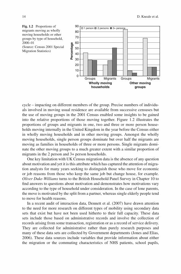
3+ personsFig. 1.2 Proportions ofmigrants moving as whollymoving households or othergroups by type of household,2000–01(Source: Census 2001 SpecialMigration Statistics)
cycle – impacting on different members of the group. Precise numbers of individu-als involved in moving usual residence are available from successive censuses butthe use of moving groups in the 2001 Census enabled some insights to be gainedinto the relative proportions of those moving together. Figure 1.2 illustrates theproportions of groups and migrants in one, two and three or more person house-holds moving internally in the United Kingdom in the year before the Census eitherin wholly moving households and in other moving groups. Amongst the whollymoving households, single person groups dominate but over half the migrants aremoving as families in households of three or more persons. Single migrants domi-nate the other moving groups to a much greater extent with a similar proportion ofmigrants in the 2 person and 3+ person households.
One key limitation with UK Census migration data is the absence of any questionabout motivation and yet it is this attribute which has captured the attention of migra-tion analysts for many years seeking to distinguish those who move for economicor job reasons from those who keep the same job but change house, for example.Oliver Duke-Williams turns to the British Household Panel Survey in Chapter 10 tofind answers to questions about motivation and demonstrates how motivations varyaccording to the type of household under consideration. In the case of lone parents,the move is motivated by the split from a partner, whereas single elderly people tendto move for health reasons.
In a recent audit of interaction data, Dennett et al. (2007) have drawn attentionto the need for more research on different types of mobility using secondary datasets that exist but have not been used hitherto to their full capacity. These datasets include those based on administrative records and involve the collection ofrecords arising from some transaction, registration or as a record of service delivery.They are collected for administrative rather than purely research purposes andmany of these data sets are collected by Government departments (Jones and Elias,2006). These data sources include variables that provide information about eitherthe migration or the commuting characteristics of NHS patients, school pupils,

1 Fertility, Living Arrangements, Care and Mobility 15
university students, asylum seekers, new migrant workers or those attending hos-pital. In some cases, registration data have much simpler structure than census dataand are only available at a relatively aggregate spatial scale but are particularly valu-able because they are produced on a regular temporal basis. In other cases, the infor-mation on migration or mobility has to be generated from the primary unit data usingtime-consuming data matching and manipulation algorithms.
One of these relatively new and unexplored administrative data sets, the PupilLevel Annual School Census (PLASC), is the focus for Joan Wilson’s researchreported in the last chapter of the book. Whilst the Census in Scotland providesdetails of the daily travel to study for students and children, similar data are notproduced for England and Wales or Northern Ireland, However, the PLASC doescollect data from each education authority in England and Wales on the location ofpupils and the schools that they attend, potentially providing an extremely usefuldata set on the journey to school. Various data sets are collected and held by theDepartment for Education and Skills (DfES) within a centralised ‘data warehouse’,including the National Pupil Database (NPD), local authority data, school level data,school workforce data and geographical data (Ewens, 2005; Jones and Elias, 2006).The NPD was established in 2002 and contains linked individual pupil records forall children in the state school system which is updated annually. Each pupil is givena unique pupil number (UPN) and has an associated set of attributes: age, gender,ethnicity, special educational needs, free school meal entitlement, key stage assess-ments, public exam results, home postcode and school attended. It is the availabilityof the last two attributes which gives the possibility of identifying various mobilitycharacteristics.
The linking of pupils from one year to the next using the UPN means that alongitudinal profile of each pupil is available whose extent depends on how longthe pupil has been in the education system. Potentially, this means that pupils canbe tracked over time and their transitions through the education system can beidentified, including their movements between schools and between different homeaddresses (Harland and Stillwell, 2007a, b). The PLASC is therefore a potentialsource of data on commuting to school, i.e. on child migration from one usual resi-dence to another and on pupil mobility between schools.
It is perhaps not surprising that these introductory comments on the content ofthe book which also attempt to provide some context to what follows, have cometo an end with a discussion about data. The Understanding Population Trends andProcesses programme, is, after all, about the analysis of secondary data sets. So,in completing this chapter, we provide a summary of the data sources that the con-tributors to this volume have used. Table 1.2 indicates that a variety of differentlongitudinal and cross-sectional survey and census data sets have been employedin the analyses that are reported in the book. No further explanation of thesedata sources is attempted here since each will be introduced in the correspondingchapter, together with the methods that have been adopted for data extraction, prepa-ration and analysis as appropriate.
In drawing this chapter to a close, we hope that readers will find the chaptersin this volume valuable as a means of understanding more about the current

16 D. Kneale et al.
Table 1.2 Main data sets used in forthcoming chapters
Chapter Author(s) Data sources
2 Simpson National Child Development Study(NCDS); British Cohort Study(BCS70)
3 Smith and Ratcliffe British Household Panel Survey(BSPS); Family ExpenditureSurvey (FES); FamilyResources Survey (FRS)
4 Hansen et al. British Birth Cohort Study(BCS70); Millennium CohortStudy (MCS); National ChildDevelopment Study (NCDS)
5 Kneale National Child Development Study(NCDS); British Cohort Study(BCS70)
6 Coast British Household Panel Survey(BHPS)
7 Young and Grundy English Longitudinal Study ofAgeing (ELSA); Office forNational Statistics (ONS)Longitudinal Study (LS);European Social Survey (ESS)
8 Boyle et al. National Child Development Study(NCDS)
9 Smith Koslowski Survey of the EuropeanCommunity Household Panel(ECHP); the European SocialSurvey (ESS); Growing Up inScotland (GUS); MillenniumCohort Study (MCS)
10 Duke-Williams 2001 Census Origin-DestinationStatistics; British HouseholdPanel Study (BHPS)
11 Wilson Pupil Level Annual School Census(PLASC)
patterns and processes of fertility, living arrangements, care and mobility, but alsofor helping to recognise what implications these trends and processes have for prac-titioners and policy makers. Both of these are primary aims of the UPTAP initiative,along with the promotion of the use of large-scale social science data sets andbuilding capacity in secondary data analysis amongst new and mid-careerresearchers. Further volumes in the series will extend our understanding bycovering social and spatial disparities (Volume 2) and ethnicity and integration(Volume 3).

1 Fertility, Living Arrangements, Care and Mobility 17
References
Alders, M.P.C. and Manting, D. (2001) Household scenarios for the European Union, 1995–2025,Genus, LVII(2): 17–48.
Allan, G., Hawker, S. and Crow, G. (2001) Family diversity and change in Britain and WesternEurope, Journal of Family Issues, 22(7): 819–837.
Appleyard, R. (1998) Emigration Dynamics in Developing Countries Volume 1–3 Sub-SaharanAfrica; Mexico, Central America and the Caribbean; South Asia and the Arab Region, UNFPAand IOM, Ashgate, Aldershot.
Axinn, W. G. and Thornton, A. (2000) The Transformation in the Meaning of Marriage, in Waite,L., Bachrach, C., Hindin, M., Thomson, E. and Thornton, A. (eds.) Ties That Bind: Perspectiveson Marriage and Cohabitation, Aldine de Gruyter, New York, pp. 147–165.
Barlow, A. (ed.) (2005) Cohabitation, Marriage and the Law: Social Change and Legal Reform inthe 21st Century, Oxford, Portland OR, Hart Publishing.
Bengston, V., Marti, G. and Roberts, R. (1991) Age group relations: generational equity andinequity, in Pillemer, K. and McCartney, K (eds.) Parent-Child Relations Across the Lifespan,Lawrence Erlbaum, Hillside (NJ), pp. 253–278.
Berrington, A.M. (2004) Perpetual postponers? Women’s, men’s and couple’s fertility intentionsand subsequent fertility behaviour, Population Trends, 117: 9–19.
Berrington, A. and Diamond, I. (2000) Marriage or cohabitation: a competing risks analysis offirst-partnership formation among the 1958 British birth cohort, Journal of the Royal StatisticalSociety, 163(2): 127–152.
Binstock, G. and Thornton, A. (2003) Separations, reconciliations, and living apart in cohabitingand marital unions, Journal of Marriage and Family, 65(2): 432–443.
Bledsoe, C.E. (2006) The demography of family reunification: from circulation to substitution inGambian Spain, MPIDR Working Paper No 2006–053, Max Planck Institute for DemographicResearch, Rostock.
Borjas, G. (2004) Increasing the supply of labour through immigration: measuring the impact ofnative-born workers, CES Working Paper No 504, www.cis.org.
Bradley, D. (2001) Regulation of unmarried cohabitation in west-European jurisdictions– determinants of legal policy, International Journal of Law, Policy and the Family,15(1): 22–50.
Buckner, L. and Yeandle, S. (2006) More than a Job Working Carers: Evidence from the2001 Census, Carers UK, London. Available from: http://www.carersuk.org/ Newsandcam-paigns/News/1159285953/MorethanaJob.pdf.
Buckner, L. and Yeandle, S. (2007) Care and Caring in EU Member States, Carers UK, London.Bumpass, L.L., Raley, R.K. and Sweet, J.A. (1995) The changing character of stepfamilies: impli-
cations of cohabitation and nonmarital childbearing, Demography, 32(3): 425–436.Champion, A.G. (2005) Population movement within the UK, in Chappell, R. (ed.) Focus on People
and Migration 2005 Edition, Palgrave Macmillan, Basingstoke, pp. 91–113.Collyer, M. (2004) The development impact of temporary international labour migration on
southern Mediterranean sending countries, Working Paper T6, Sussex Centre for MigrationResearch, University of Susses, Brighton.
Coombes, M.G. and Raybould, S. (2001) Commuting in England and Wales: ‘people’ and ‘place’factors, European Research in Regional Science, 11(1): 111–133.
Coontz, S. (2004) The world historical transformation of marriage, Journal of Marriage and Fam-ily, 66(4): 974–979.
Coyle, A. (2005) Changing times: flexibilization and the re-organization of work in feminizedlabour markets, Sociological Review, 53: 73–88.
Darroch, J.E., Landry, D.J. and Oslak, S. (1999) Pregnancy rates among US women and theirpartners in 1994, Family Planning Perspectives, 31: 122–126+136.
De Graaf, P.M. and Kalmijn, M. (2003) Alternative routes in the remarriage market: competing-riskanalyses of union formation after divorce, Social Forces, 81(4): 1459–1598.

18 D. Kneale et al.
De Jong Gierveld, J. (2004) Remarriage, unmarried cohabitation, living apart together: part-ner relationships following bereavement or divorce, Journal of Marriage and Family, 66(1):236–243.
De Vaus, D, Qu, L. and Weston, R. (2005) The disappearing link between premarital cohabitationand subsequent marital stability, 1970–2001, Journal of Population Research, 22(2): 99–118.
Dennett, A. and Stillwell, J. (2008) Internal migration in Great Britain – a district level analysisusing 2001 Census data, Working Paper 01/08, School of Geography, University of Leeds,Leeds.
Dennett, A., Stillwell, J. and Duke-Williams, O. (2007) Interaction data sets in the UK: an audit,Working Paper 07/03, School of Geography, University of Leeds, Leeds.
Dex, S, Joshi, H, Macaran, S. and McCulloch, A. (1998) Employment after childbearing andwomen′s subsequent labour force participation: evidence from the British 1958 birth cohort,Oxford Bulletin of Economics and Statistics, 60: 79–98.
Duncan, G. J, Wilkerson, B. and England P. (2006) Cleaning up their act: The effects of marriageand cohabitation on licit and illicit drug use, Demography, 43(4): 691–710.
Dush, C.M.K. and Amato, P.R. (2005) Consequences of relationship status and quality for subjec-tive well-being, Journal of Social and Personal Relationships, 22(5): 607–628.
Dustmann, C, Fabbri, F, Preston, I. and Wadsworth, J. (2003) The Local Labour Market Effects ofImmigration in the UK, Home Office Online Report 06/03, London.
Edwards, M.E. (2002) Education and occupations: reexamining the conventional wisdom aboutlater first births among American mothers, Sociological Forum, 17: 423–443.
Eekelaar, J. and Maclean, M. (2004) The obligations and expectations of couples within families:three modes of interaction, Journal of Social Welfare and Family Law, 26(2): 117–130.
Eggebeen, D.J. (2005) Cohabitation and exchanges of support, Social Forces, 83(3): 1097–1110.Elizabeth, V. (2000) Cohabitation, marriage, and the unruly consequences of difference, Gender
and Society, 14(1): 43–56.Elliott, J. (2005) Using Narrative in Social Research, SAGE Publications Limited, London.Ermisch, J. and Francesconi, M. (2000) The increasing complexity of family relationships: life-
time experience of lone motherhood and stepfamilies in Great Britain, European Journal ofPopulation, 16(3): 235–250.
ESRC (2006) Changing Household and Family Structures and Complex Living Arrangements,Economic and Social Research Council. Swindon.
Eurostat (2004) EUROPOP 2004 – Summary Note on Assumptions and Methodology for Inter-national Migration, Working Paper for the Ageing Working Group on the EPC, ESTAT/F1-/POP/19(2004)/GL, Luxembourg.
Ewens, D. (2005) The national and London pupil datasets: an introductory briefing for researchersand research users, Data Management and Analysis Group, Greater London Authority.
Fischer, P, Martin, R. and Straubhaar, T. (1997) Interdependencies between development andmigration, in Hammar, T., Brochmann, G., Tamas, K. and Faist, T. (eds.) InternationalMigration, Immobility and Development: Multidisciplinary Perspectives, Berg Publishers,Oxford.
Flood, M. (2007) Involving men in gender policy and practice, Critical Half: Bi-Annual Journal ofWomen for Women International, 5: 9–15.
Flowerdew, R. and Hamad, A. (2004) The relationship between marriage, divorce and migrationin a British data set, Journal of Ethnic and Migration Studies, 30(2): 339–351.
Frost, M. and Shepherd, J. (2004) New methods of assessing service provision in ruralEngland, in Stillwell, J. and Clarke, G. (eds.) Applied GIS and Spatial Analysis, Wiley,Chichester.
Gibson-Davis, C.M, Edin, K. and McLanahan, S. (2005) High hopes but even higher expectations:the retreat from marriage among low-income couples, Journal of Marriage and the Family,67(5): 1301–1312.
Giddens, A. J. (1993) The Transformation of Intimacy: Love, Sexuality and Eroticism in ModernSocieties, Polity Press, Cambridge.

1 Fertility, Living Arrangements, Care and Mobility 19
Gillis, J. (2004) Marriages of the mind, Journal of Marriage and Family, 66(4): 988–991.Glaser, K, Askahm, J. et al. (2005) Married or single: which shall I tick? Findings from a Study of
BHPS Marital Status Data, BHPS 2005 Conference, Colchester.Gonzalez, M.-J. and Jurado-Guerrero, T. (2006) Remaining childless in affluent economies: a com-
parison of France, West Germany, Italy and Spain, 1994–2004, European Journal of Popula-tion, 22: 317–352.
Goodman, A, Kaplan, G. and Walker, I. (2004) Understanding the effects of early motherhoodin Britain: the effects on mothers, IFS Working Paper 04/18, Institute for Fiscal Studies,London.
Greene, M.E. and Biddlecom, A.E. (2000) Absent and problematic men: demographic accounts ofmale reproductive histories, Population and Development Review, 26: 81–115.
Guzzo, K.B. (2006) The relationship between life course events and union formation, Social Sci-ence Research, 35(2): 384–408.
Hadfield, L., Rudoe, N. and Sanderson-Mann, J. (2007) Motherhood, choice and the British media:a time to reflect, Gender and Education, 19: 255–263.
Hall, S.S. (2006) Marital meaning: exploring young adults’ belief systems about marriage, Journalof Family Issues, 27(10): 1437–1458.
Harden, A., Brunton, G., Fletcher, A., Oakley, A., Burchett, H. and Backhans, M. (2006) Youngpeople, pregnancy and social exclusion: A systematic synthesis of research evidence to iden-tify effective, appropriate and promising approaches for prevention and support, The Evidencefor Policy and Practice Information and Co-ordinating Centre (EPPI-Centre), University ofLondon, London.
Harland, K. and Stillwell, J. (2007a) Commuting to school in Leeds: how useful is the PLASC?Working Paper 07/02, School of Geography, University of Leeds, Leeds.
Harland, K. and Stillwell, J. (2007b) Using PLASC data to identify patterns of commuting toschool, residential migration and movement between schools in Leeds, Working Paper 07/03,School of Geography, University of Leeds, Leeds.
Haskey, J. (2001) Demographic aspects of cohabitation in Great Britain, International Journal ofLaw, Policy, and the Family, 15(1): 51–67.
Heuveline, P. and Timberlake, J.M. (2004) The role of cohabitation in family formation:the United States in comparative perspective, Journal of Marriage and Family, 66(5):1214–1230.
Holzmann, R. and Munz, R. (2004) Challenges and Opportunities of International Migration forthe EU, Its Member States, Neighbouring Countries and Regions: A Policy Note, World Bank,Washington DC and Institute for Futures Studies, Stockholm.
Hotz, V. J., MCelroy Williams, S. and Sanders, S.G. (2004) Teenage Childbearing and Its Lifecy-cle Consequences: Exploiting a Natural Experiment, Department of Economics, University ofCalifornia (UCLA), Los Angeles.
Hunter, J. (2005). Report on Cognitive Testing of Cohabitation Questions. Study Series Report:Survey Methodology #2005-06, U.S. Census Bureau, Statistical Research Division: 18.
Imamura, M., Tucker, J., Hannaford, P., Oliveira Da Silva, M., Astin, M., Wyness, L.,Bloemenkamp, K.W.M., Jahn, A., Karro, H., Olsen, J. and Temmermen, M. (2007) Factorsassociated with teenage pregnancy in the European Union countries: a systematic review, Euro-pean Journal of Public Health, 17: 630–636.
Jamieson, L., Anderson, M., McCrone, D., Bechhofer, F., Stewart, R., and Li, Y (2002) Cohabita-tion and commitment: partnership plans of young men and women, Sociological Review, 50(3):356–377.
Jefferies, J. (2005) The UK Population: Past, Present and Future. Focus on People and Migration,Office for National Statistics, London.
Jones and Elias, P. (2006) Administrative data as research resources: a selected audit, WorkingPaper, Warwick Institute for Employment Research, Warwick.
Joshi, H. (2002) Production, reproduction, and education: women, children and work in a Britishperspective, Population and Development Review, 28: 445–474.

20 D. Kneale et al.
Joshi, H. (2007) Social Polarisation in Reproduction. From Boom to Bust: Fertility, Ageing andDemographic Change, CentreForum, London.
Kapur, D. and McHale, J. (2005) Give Us Your Best and Brightest: the Global Hunt for talent andits Impact on the Developing World, Center for Global Development, Washington DC.
Kenney, C.T. and McLanahan, S.S. (2006) Why are cohabiting relationships more violent thanmarriages? Demography, 43(1): 127–140.
Kiernan, K. (2000) European perspectives on union formation, in Waite, L. (ed.) The Ties thatBind: Perspectives on Marriage and Cohabitation, Aldine de Gruyter, New York, pp. 40–58.
Kiernan, K. (2001) The rise of cohabitation and childbearing outside marriage in western Europe,International Journal of Law, Policy and the Family, 15(1): 1–21.
Knab, J. and McLanahan, S. (2006) Measuring cohabitation: does how, when and who you askmatter? in Hofferth, S.L. and Casper, L.M. (eds.) Handbook of Measurement Issues in FamilyResearch, Lawrence Erlbaum & Associates, New Jersey, pp. 19–33.
Lampard, R. and Peggs, K. (1999) Repartnering: the relevance of parenthood and gender tocohabitation and remarriage among the formerly married, British Journal of Sociology, 50(3):443–465.
Lauster, N.T. (2006) A room of one′s own or room enough for two? Access to housing and newhousehold formation in Sweden, 1968–1992, Population Research and Policy Review. 25(4):329–351.
Lehrer, E.L. (2004) The role of religion in union formation: an economic perspective, PopulationResearch and Policy Review, 23(2): 161–185.
Lesthaeghe, R. and Moors, G. (1995) Living arrangements and parenthood: do values matter? in deMoor, R.A. (ed.) Values in Western Societies, Tilburg University Press, Tilburg, pp. 217–250.
Lesthaeghe, R. and Neels, K. (2002) From the first to the second demographic transition - aninterpretation of the spatial continuity of demographic innovation in France, Belgium andSwitzerland, European Journal of Population, 18(4): 225–260.
Levin (2004) Living apart together: a new family form, Current Sociology, 52(2): 223–240.Lewis, J. and Campbell, M. (2007) UK work/family balance policies and gender equality
1997–2005, Social Politics, 14: 4–30.Levitt, P. (2006) Transnational migration: conceptual and policy challenges, in Tamas, K. and
Palme, J. (eds.) Globalising Migration Regimes: New Challenges to Transnational Coopera-tion, Ashgate, Avebury.
Lewis, J. (1999) Marriage, Cohabitation and the Law: Individualism and Obligation, Lord Chan-cellor’s Department, London.
Lewis, J. (2001a) Debates and issues regarding marriage and cohabitation in the British and Amer-ican literature, International Journal of Law, Policy, and the Family, 15(1): 159–184.
Lewis, J. (2001b) The End of Marriage? Individualism and Intimate Relations, E Elgar Pub, Chel-tenham.
Lewis, J. and Campbell, M. (2007) UK work/family balance policies and gender equality1997–2005, Social Politics, 14: 4–30.
Liefbroer, A.C. and Dourleijn, E. (2006) Unmarried cohabitation and union stability: test-ing the role of diffusion using data from 16 European countries, Demography, 43(2):203–221.
MacLean, M. and Eekelaar J. (2004) The obligations and expectations of couples within families:three modes of interaction, Journal of Social Welfare and Family Law, 26(2): 117–130.
Mahay, J. and Lewin, A.C. (2007) Age and the desire to marry, Journal of Family Issues, 28(5):706–723.
Manning, W.D., Longmore, M.A. and Giordano, P.C. (2007) The changing institution of marriage:adolescents’ expectations to cohabit and to marry, Journal of Marriage and Family, 69(3):559–575.
Manning, W.D. and Smock, P.J. (2005) Measuring and modeling cohabitation: new perspectivesfrom qualitative data, Journal of Marriage and Family, 67(4): 989–1002.
Manting, D. (1996) The changing meaning of cohabitation and marriage, European SociologicalReview, 12(1): 53–65.

1 Fertility, Living Arrangements, Care and Mobility 21
Marcussen, K. (2005) Explaining differences in mental health between married and cohabitingindividuals, Social Psychology Quarterly, 68(3): 239–257.
Massey, D., Arango, J, Hugo, G., Kouaouci, A., Pelegrino, A. and Taylor, J. (1998) Worlds inMotion: Understanding International Migration at the End of the Millenium, Clarendon Press,Oxford.
Mastekaasa, A. (2006) Is marriage/cohabitation beneficial for young people? Some evidence onpsychological distress among Norwegian college students, Journal of Community and AppliedSocial Psychology, 16(2): 149–165.
Morgan, P.M. (2000) Marriage-lite: The Rise of Cohabitation and its Consequences, Institute forthe Study of Civil Society, London.
Murphy, M. (2000) Cohabitation in Britain, Journal of the Royal Statistical Society, 163(2):123–126.
Musick, K. (2007) Cohabitation, nonmarital childbearing, and the marriage process, DemographicResearch, 16(9): 249–286.
Office for National Statistics (2007) Live births: age of mother, 1961 onwards (England and Wales),Health Statistics Quarterly, 37: 36.
Oppenheimer, V.K. (2003) Cohabiting and marriage during young men′s career-development pro-cess, Demography, 40(1): 127–149.
Osborne, C. (2005) Marriage following the birth of a child among cohabiting and visiting parents,Journal of Marriage and Family, 67(1): 14–26.
Phillipson, C. (1998) Reconstructing Old Age: New Agendas in Social Theory and Practice, Sage,London.
Pleck, J.H. (2007) Why could father involvement benefit children? Theoretical perspectives,Applied Developmental Science, 11: 196–202.
Poot, J., Gorter, C. and Nijkamp, P. (eds.) (1998) Crossing Borders: Regional and Urban Perspec-tives on International Migration, Ashgate, Aldershot UK.
Power, C. and Elliott, J. (2006) Cohort profile: 1958 British birth cohort (National Child Develop-ment Study), International Journal of Epidemiology, 35: 34–41.
Probert, R. (2004) Cohabitation in twentieth century England and Wales: law and policy, Law andPolicy, 26(1): 13–32.
Raley, R.K. (2001) Increasing fertility in cohabiting unions: evidence for the second demographictransition in the United States? Demography, 38(1): 59–66.
Reed, J.M. (2006) Not crossing the “extra line”: how cohabitors with children view their unions,Journal of Marriage and Family, 68(5): 1117–1131.
Rendall, M.S., Clarke, L., Peters, H.E., Ranjit, N. and Verropoulou, G. (1999) Incomplete reportingof men′s fertility in the United States and Britain: a research note, Demography, 36, 135–144.
Rendall, M.S., Couet, C., Lappegard, T., Robert-Bobee, I., Romsen, M. and Smallwood, S. (2005)First birth by age and education in Britain, France and Norway, Population Trends, 121: 27–34.
Rendall, M.S. and Smallwood, S. (2003) Higher qualifications, first birth timing and further child-bearing in England and Wales, Population Trends, 111: 18–27.
Rossi, P. (1955) Why Families Move: A Study in the Social Pschologyof Urban Residential Mobil-ity, Free Press, Glencoe, Illinois.
Sarkadi, A., Kristiansson, R., Oberklaid, F. and Bremberg, S. (2008) Fathers’ involvement andchildren’s developmental outcomes: a systematic review of longitudinal studies, Acta Paedia-tricia, 97: 153–158.
Sassler, S. (2004) The process of entering into cohabiting unions, Journal of Marriage and Family,66(2): 491–505.
Scott, J. (1999) Family Change: Revolution or Backlash in Attitudes? in McRae, S. (ed.)Changing Britain: Families and households in the 1990s, Oxford University Press, Oxford,pp. 68–99.
Seltzer, J.A. (2000) Families formed outside of marriage, Journal of Marriage and Family, 62(4):1247–1268.
Seltzer, J.A. (2004) Cohabitation in the United States and Britain: demography, kinship, and thefuture, Journal of Marriage and Family, 66(4): 921–928.

22 D. Kneale et al.
Seltzer, J. A., Bachrach, C.A. Bianchi, S.M., Bledsoe, C.H., Casper, L.M., Chase-Lansdale, P.L.,et al. (2005) Explaining family change and variation: challenges for family demographers,Journal of Marriage and Family, 67(4): 908–925.
Skeldon, R. (1997) Migration and Development: A Global Perspective, Addison Wells/Longman,Harlow.
Smallwood, S. and Chamberlain, J. (2005) Replacement fertility: What has it been and what doesit mean? Population Trends, 119: 16–27.
Smock, P. J. and Manning, W.D. (2004) Living together unmarried in the United States: demo-graphic perspectives and implications for family policy, Law and Policy, 26(1): 87–118.
Smock, P. J., Manning, W.D. and Porter, M. (2005) “Everything’s there except money”: Howmoney shapes decisions to marry among cohabitors, Journal of Marriage and Family, 67(3):680–696.
Social Exclusion Unit (1999) Teenage Pregnancy, Social Exclusion Unit, London.Stafford, L., Kline, S.L., and Rankin, C.T. (2004) Married Individuals, cohabiters, and cohabiters
who marry: a longitudinal study of relational and individual well-being, Journal of Social andPersonal Relationships, 21: 231–248.
Stillwell, J. and Duke-Williams, O. (2003) A new web-based interface to British census of popu-lation origin-destination statistics, Environment and Planning A, 35: 113–132.
Tamas, K. and Munz, R. (2006) Labour Migrants Unbound? EU Enlargement, Transitional Mea-sures and Labour Market Effects, Institute for Futures Research, Stockholm.
Terry, D.F. and Wilson, S.R. (eds.) (2005) Beyond Small Change: Making Migrant RemittancesCount, Inter-American Development Bank, Washington DC.
Therborn, G. (2007) Is there a future for the family?, Public Policy Research, 14(1): 41–46.Thornton, A., Axinn, W.G. and Xie, Y. (2007) Marriage and Cohabitation, University of Chicago
Press, Chicago.Thornton, A. and Young-DeMarco, L. (2001) Four decades of trends in attitudes toward family
issues in the United States: the 1960s through the 1990s, Journal of Marriage and Family,63(4): 1009–1037.
Ungerson, C. and Yeandle, S. (eds.) (2007) Cash for Care in Developed Welfare States, PalgraveMacmillan, London.
UNICEF (2001) A League Table of Teenage Births in Rich Nations, UNICEF Innocenti ResearchCentre, Florence.
United Nations (2005) World Population Prospects. The 2004 Revision, UN, NewYork.Van de Kaa, D.J. (1987) Europe’s second demographic transition, Population Bulletin, 42: 1–59.Wagner, M. and Weib, B. (2006) On the variation of divorce risks in Europe: findings from a meta-
analysis of European longitudinal studies, European Sociological Review, 22(5): 483–500.Walker, A. (ed.) (1996) The New Generational Contract: Intergenerational Relations, Old Age and
Welfare, Routledge, London.White, N.R. (2003) Changing conceptions: young people’s views of partnering and parenting, Jour-
nal of Sociology, 39(2): 149–164.Williams, F. (2004) Trends in women’s employment, domestic service, and female migration:
changing and competing patterns of solidarity, in Knijn, T. and Komter, A. (eds.) SolidarityBetween the Sexes and Generations: Transformations in Europe, Edward Elgar, Aldershot,pp. 210–218.
Yeandle, S. (2007) Carers, employers and the state: clarifying the social contract, Paper presentedto the Caregivers: Essential Partners in Care Conference (FICCDAT), Toronto, Canada, 16–19June.
Yeandle, S., Bennett, C., Buckner, L., Suokas, A. and Shipton, L. (2006a) Who Cares Wins: theSocial and Business Benefits of Supporting Employed Carers, Carers UK, London.
Yeandle, S., Buckner, L. and Shipton, S. (2006b) Local Challenges in Meeting Demand for Domi-ciliary Care – Synthesis Report, Centre for Social Inclusion, Sheffield Hallam University,Sheffield.
Zimmermann, A.C. and Easterlin, R.A. (2006) Happily ever after? Cohabitation, marriage, divorce,and happiness in Germany, Population and Development Review, 32(3): 511.

Chapter 2Delayed Childbearing and Childlessness
Roona Simpson
Introduction
Fertility patterns have changed significantly in most European countries since the1960s. Although there are important differences both between and within countriesin the pace of decline, by the 1990s fertility reached below replacement levels acrossEurope, with several countries experiencing lowest-low levels (less than 1.31 chil-dren per woman) (European Commission 2006a). Declining fertility is one aspectof an inter-related package of demographic trends that both reflect and constitutea transformation of the context in which people may or may not partner and par-ent. Debates within demography over the causes and consequences of the seconddemographic transition have been paralleled by sociological debate on the impactof individualism on personal life. This chapter considers these debates in relation tofindings from analysis of the British cohort studies looking at changes over time inthe propensity to delayed childbearing.
Within demographic debate a ‘post-materialist values’ perspective contends thatchanges in social and demographic behaviour have been driven by a growth invalues of self-realisation in the context of a decline in tradition and diminishing con-straints (Van de Kaa, 1987; Lesthaeghe, 1995; Leete, 1998). Similarly, much soci-ological theorising on the changing character of intimacy and partnership empha-sises an increase in behavioural options in the context of increasing individualism(Bauman, 2000; Giddens, 1992; Beck and Beck-Gernsheim, 1995, 2002). Withinthese debates, increasing childlessness has featured as a signifier of a ‘choice biogra-phy’ or, in more pessimistic accounts, as indicative of self-interested individualism.
Whereas the decline of fertility below replacement level was previously viewedas the most important feature of the demographic transition (Van de Kaa, 1987),the postponement of first births is now portrayed as the most radical transformation(Lesthaeghe and Neels 2002: 33). While second and higher-order births are beingpostponed as well, this is mostly as a consequence of first-birth postponement rather
R. Simpson (B)Centre for Research on Families and Relationships, University of Edinburgh, UKe-mail: [email protected]
J. Stillwell et al. (eds.), Fertility, Living Arrangements, Care and Mobility, UnderstandingPopulation Trends and Processes 1, DOI 10.1007/978-1-4020-9682-2 2,C© Springer Science+Business Media B.V. 2009
23

24 R. Simpson
than a manifestation of change in birth intervals (Sobotka, 2004). There is somedebate in the literature as to the extent to which delayed childbearing is related toincreased childlessness, or constitutes a ‘postponement transition’ towards a latefertility regime (Kohler et al., 2002: 659–661).
There are numerous factors proposed in the literature to explain delayed child-bearing and much empirical research investigating their impact. These include thespread of access to modern contraception (e.g. Murphy, 1992, 1993), changes inparticipation in education (e.g. Kohler et al., 2002) and employment (e.g. Brewsterand Rindfuss, 2000), the wider economic context (e.g. Bagavos and Martin, 2000)as well as the shifting character of intimacy and partnership relations in the con-text of shifts in balances of power between men and women (e.g. Lesthaeghe, 1995;Oppenheimer, 1994). However, many factors are clearly interconnected, with theirrelative impact difficult to quantify. Thus, in relation to contraception there arevarying emphases on the interpretation of this as a technical factor addressing ademand for birth control (e.g. Castles, 2003) or as a precursor to broader behaviouraland cultural changes, including changing partnership patterns more generally (e.g.Van de Kaa, 1994: 114). As well as understanding this as a necessary preconditionfor various other changes, some authors emphasise the social and psychological sig-nificance for women of the ability to control their fertility (Presser, 2001; Hakim,2003). The expansion of post-secondary education in recent decades in a contextof an increased emphasis on educational attainment in securing stable employ-ment, adequate income and career development, has been interpreted as impactingdirectly on fertility. ‘Being in education’, during which students usually lack ade-quate resources and with future employment conditions uncertain, strongly reducesthe likelihood of having a first child (e.g. Blossfeld, 1995; Hoem, 2000). However,as well as delay attributable to time spent in education, this influences the timing ofparenthood indirectly, through increased career opportunities or a less traditional orfamily-centred value orientation (Oppenheimer, 1994).
Educational level is clearly linked to employment, associated with an enhancedposition in the labour market. Much attention has focused on the demise of a ‘malebreadwinner model’ and the increasing likelihood of women combining caring forchildren with participation in the labour market. Debates about the opportunity costsof childbearing for women and conflict between career aspirations and motherhoodare prevalent in the demographic literature. The ‘positive turn’ in many countries,with higher fertility associated with higher female labour force participation, hasdrawn attention to specific policy contexts within which individuals seek to balancework and family aspirations (Esping-Anderson, 1999; McDonald, 2000a; Castles,2003; Hobson and Olah, 2006a). Birth timing and spacing may be key strategiesadopted to reconcile these (De Cooman et. al., 1987; Brewster and Rindfuss, 2000).Empirical studies demonstrate substantial differences in first birth timing accordingto the level of education, with highly educated women postponing childbearing to alarger extent than women with less education who often continue to have childrenat early ages (Gustaffson et al., 2002; Joshi, 2002; Sobotka, 2004).
There has been much recent sociological attention to new social risks conse-quent on various inter-related changes occurring as part of a shift to a post-industrial

2 Delayed Childbearing and Childlessness 25
society. One aspect of this is the extent to which risk aversion applies to the personalsphere and influences the likelihood of people embarking on partnership or parent-ing (e.g Beck, 1999; Taylor-Gooby, 2004; Lewis, 2006). There has also been atten-tion to the impact of global restructuring and welfare state retrenchment of recentdecades in demographic debates, with unemployment for example analysed as a fac-tor that increases economic uncertainty and discourages union formation and parent-hood (see Kohler et al., 2002; Meron and Widmer, 2002; Hobson and Olah, 2006b).Sobotka argues that the available evidence suggests the influences of uncertainty onfirst birth timings differ in time, across countries, by types of uncertainty and with adiffering impact on various population groups (Sobotka, 2004: 21), citing in illustra-tion a study of fertility in England and Wales (De Cooman et al., 1987) which foundfertility reactions to economic change varying by stage in family formation, withlabour market conditions influencing timing rather than the quantum of fertility.
Various inter-related changes have resulted in considerable transformations infamily and household formations, as a now familiar list of trends including thedelay and decline in marriage, the separation of marriage and reproduction (bothchildless marriage and non-marital fertility) and an increase in unconventional liv-ing arrangements such as solo living, demonstrate. These are occurring alongsidea relative lack of change in some traditional elements of partnership and parent-ing, including in gendered divisions of labour (see Folbre, 1994; Hoshchild, 2001).Trends to delayed childbearing and increased childlessness in recent decades areclearly not independent of trends in partnership formation and dissolution. There isempirical data supporting the idea that more complex partnership patterns are asso-ciated with late entry into parenthood (e.g. Olah, 2005). It is, however, transforma-tions in ways of interacting within relationships, rather than changing structures perse, which are argued as having profound consequences for fertility. Whereas someauthors contend these changes reflect an increasing emphasis on self-fulfilment(e.g. Van de Kaa, 2004), others have interpreted this in terms of women’s greaterindependence allowing them to set higher standards in relation to partnership (e.g.Oppenheimer, 1994), including expectations around gender equity in the domesticsphere (e.g. McDonald, 2000b; Berrington, 2004; Wasoff and Dey, 2007).
There is considerable debate around which are the most significant factors driv-ing contemporary changes in both partnership and parenting, and how it may bepossible to identify primary factors (Kohler et al., 2002; Caldwell and Schindlmayr,2003, Hobcraft, 2004). Several authors have also questioned individualist expla-nations of demographic behaviour as the outcome of a ‘freeing’ of agency fromchanging social conditions, arguing rather that individual choices are inseparablefrom the social contexts, including the structural process and cultural mores, withinwhich they are made (Irwin, 2005; Smart, 2007).
Most research on fertility focuses on women, to the empirical neglect of men(Greene and Biddlecom, 2000: 81). This may be in part due to the greater reliabil-ity of reported fertility by women. Previous research suggests some unreliability inmen’s reporting of children, especially of non-marital births; for example Rendallet al. (1999). An evaluation of men’s retrospective fertility histories from the BritishHousehold Panel Study found only 60 of men’s births from a previous marriage

26 R. Simpson
were reported per 100 of women’s births, with women’s fertility reports matchingbirth registration statistics (Rendall et al., 1999). Survey data do not lend them-selves readily to explorations of the motivations and meanings individuals ascribeto statuses such as childlessness. Yet qualitative research studies on the experienceof childlessness in recent decades similarly focuses on women (see Veevers, 1980;Cameron, 1997; Lisle, 1999). Such a focus, as well as neglecting the experience ofmen, can reinforce a view of women as primarily reproductive (see Watkins, 1993).Furthermore, despite an emphasis in much of the sociological and demographic lit-erature on ‘choice’ biographies, the emphasis on women risks ignoring the extentto which preferences and decision-making around parenthood are negotiated at thelevel of the couple. This reinforces the importance of considering contemporarychange in the partnership context in which decisions about childbearing are beingmade.
In common with many other industrialized nations, there have been significantchanges in the timing and context of partnership and parenthood in Britain in recentdecades. In 1971, the average age of first marriage in England and Wales was 25for men and 23 for women. However, by 2003, this had increased to 31 for menand 29 for women. Alongside this delay in marriage there has been a huge increasein cohabitation. Non-marital cohabitation amongst those under 60 in Great Britaindoubled between 1986 (the earliest year for which data are available on a consis-tent basis) and 2006, from 11% to 24% for men, and 13 to 25% for women (ONS,2008). There has also been a dramatic increase in recent decades of men and womenliving alone at ages conventionally associated with co-resident partnership and par-enthood: over the past two decades the proportion of people living alone has dou-bled, from 7% to 14% of men aged 25–44 and from 4% to 8% of women in this agegroup (ONS, 2008: 19). These all have implications for the context of childbearing.Births by unmarried women accounted for 42% of all births in the United Kingdomin 2004, compared to an EU (15 countries) average of 33% (European Commission,2006b). For women, the average age of first birth rose from 24 in the early 1970s to28 in 2006, and this is even higher for first births within marriage, with an averageage of 30 in 2006 (ONS, 2008: 24). There has also been an increase in delayed child-bearing and childlessness. Whereas around 16% of women born in 1931 remainedchildless at 35, this compares with a quarter of women born in 1971. The proportionof women remaining childless at 45 has risen from 14% of women born in 1931 tojust under a fifth (19%) of those born in 1961, the latest cohort to reach the end oftheir childbearing years (ONS, 2008: 24).
Figure 2.1 illustrates changes over time in the percentages of women remainingchildless, having only one child, or large families (four or more children). Figuresfor 1920 are included to demonstrate that these figures are not unprecedented, withan average age of first birth of 28.7 for women born in 1920.
The previous discussion outlines the predominant factors identified in the liter-ature with delayed childbearing. However, as noted above, there is relatively littleattention to that of men. The following section reports analysis of the British cohortstudies looking at men and women born in 1958 and 1970. As well as comparisonsby sex, this inter-cohort analysis allows comparisons across time, thereby providing

2 Delayed Childbearing and Childlessness 27
No children 1 child 4 or more children25
20
15
10
5
0
Wo
man
(%
)
196019551950194519401920
Year
Fig. 2.1 Completed familysize, selected cohorts (%)(Source: ONS Cohort SeriesFM1 No. 35, Table 10.5)
a picture of the impact of social change on the lives of cohort members. Previousanalyses of the cohort studies demonstrate changes across a range of domains suchas education, employment, health and family life, which reflect the wider socialcontext in which these changes were experienced (Ferri et al., 2003). Those bornin 1958 will have experienced their early adulthood during the 1980s, a very dif-ferent political, social and economic context from those born in 1970: whereas the1958 cohort initially experienced a buoyant labour market but faced worse condi-tions as they got older, the opposite occurred for those born in 1970. Rising livingstandards in recent decades have been accompanied by increasing polarisation interms of wage inequality. Cohort members remaining childless in their early thirtieswill also have experienced this in differing circumstances, those born in 1958 in theearly 1990s, and those born in 1970 in the early twenty-first century.
Data and Methods
The National Child Development Study (NCDS) and British Cohort Study (BCS)are longitudinal surveys following a sample of individuals born in Great Britainbetween 3–9 March 1958 and 5–11 April 1970 respectively. Surveys to monitor theeducational, physical and social development of these cohorts have taken place atvarying intervals, with data collected at birth, 7, 11, 16, 23, 33, 41/42 and 46/47forthe NCDS and at birth, 5, 10, 16, 26, 29/30 and 33/34 for the BCS. Earlier stagesof the studies were conducted by various organisations, however data collectionfor these and other birth cohort studies is now the responsibility of the Centre forLongitudinal Studies, Institute of Education, University of London. Full fertilityhistories were produced for the NCDS cohort at age 33/34 (see Di Salvo, 2005), andthese were drawn on in the analysis presented below.1
Longitudinal data enabling the opportunity to investigate demographic eventswithin a life course perspective, however, are subject to attrition, and approximately
1Fertility histories are also collected at age 23 years for the NCDS cohort; although a cross-sectional approach was favoured for the analysis of NCDS data in this study.

28 R. Simpson
two thirds of those taking part in the birth survey were interviewed in their early thir-ties. Previous analyses of the response bias arising from this suggests it is the mostsocio-economically disadvantaged that are over-represented amongst those lost overtime (for further detail see Shepherd, 1995; Plewis et al., 2004). Both samples alsounder-represent those who began child-bearing in their teens (Berrington, 2003).The analysis assumes any attrition bias is similar in both surveys.
There are 11,407 men and women aged 33 in the NCDS5 cohort, and 11,261 aged30 in the BCS 2000 cohort. The findings presented below report analysis conductedon individuals in these sweeps who were also present at ages 33/34 (BCS 2004) (n =9,665), in order to conduct comparisons by cohort at exact age 33. Survival analyseswere conducted on both cohorts, subsequent to cleaning the data to address thosewith missing/incomplete birth dates. As the focus of this chapter is on postponedfertility it only considers biological children, and childlessness is defined as nothaving had a live birth; those classified as childless may include respondents withadopted or step-children.
The analysis considered several variables identified as important in the litera-ture.2 As noted above, previous research has attributed fertility postponement tochanges in education and employment (particularly for women), and partnershipformation. However, these are mediated by social class (Berrington, 2003). The fol-lowing section reports the results of analyses looking at childlessness by sex inrelation to social class background identified using the occupational social class(Registrar General’s definition) of the cohort member’s father (or father figure) atage 16; educational attainment by age 33– those with no qualifications, school-level qualifications (including A/S level and their NVQ equivalents) and tertiarylevel qualifications, including Higher qualifications, degrees and NVQ equivalents(4–6); current economic activity-looking at those working full-time or part-time(whether employee/self-employed), unemployed and seeking work, permanentlysick/disabled, or looking after home/family; and current marital and (co-residential)partnership status.3
2Initial analysis was carried out looking at religiosity. The Second Demographic Transitionattributes declining fertility to, inter alia, a growth of values of self-realisation and freedom fromtraditional forces of authority such as religion and previous research reports a correlation betweenincreased religious activity and more traditional attitudes to family (e.g. Berrington and Diamond,2000; Olah, 2005). However, while there was a decline in religiosity evident (only 11 per centof the 1970-born cohort who defined themselves as having a religion attended services at leastmonthly, compared with 30 per cent of the 1958 cohort), there was no significant association withremaining childless in one’s early thirties.3Marital status distinguishes the currently married (whether first or subsequent), the previouslymarried (the separated or divorced, as well as the very small numbers widowed in each cohort),and the never-married. Partnership status distinguishes those currently cohabiting: partnership his-tories record relationships in which respondents ‘lived with someone as a couple’ for a month ormore. However, as Murphy (2000) observes, assuming all co-residential partnerships as equivalentraises several issues: these may differ not just in de jure status, but in terms of the meanings andmotivations these hold for respondents.

2 Delayed Childbearing and Childlessness 29
The Propensity to Childlessness Among YoungAdults – Differences by Sex and Changes Over Time
The analysis compares the propensity amongst men and women to remain child-less by exact age 33, considering this in relation to various socio-economic charac-teristics and circumstances. Comparisons are also made with those who have hadchildren at the same age, to provide a broad overview. As noted above cohort mem-bers who remain childless at 33 will have experienced this in somewhat differentcontexts.
Delayed Childbearing by Sex
As Figure 2.2 illustrates, there are significant differences by sex, with larger propor-tions of men remaining childless at age 33 compared with women in both cohorts.Thus, a third of men in the 1958 cohort remained childless at 33 compared to justunder a quarter (24%) of women at the same age. For the 1970 cohort the figureswere over half (51%) of men compared with less than two fifths (36%) of women atthe same age.
These figures also illustrate a dramatic increase in childlessness amongst adultsin their early thirties in just 12 years, particularly for men. The median age of firstbirth for women has increased from 27 to 30 and for men from 30 to 34. Previousanalysis of the cohort studies (Berrington, 2003) finds that, alongside an increase inmedian age across cohorts, similar proportions (around 10%) became teenage moth-ers, indicating increasing polarisation between women in relation to age at first birth.
Delayed Childbearing by Social Class Background
As Figure 2.3 illustrates (see also Table 2.1), there are significant differences inthe propensity to remain childless at age 33 by social class background, defined
60
50
40
30
20
10
0
Ch
ildle
ss (
%)
19701958
3324
51
36
Year
Male Female
Fig. 2.2 Childlessness at 33by sex and cohort (%)(Source: Author’scalculations based on surveydata)

30 R. Simpson
I and II IIInm IIIm IV and V No father figure80
70
60
50
40
30
20
10
0
Ch
ildle
ss (
%)
1958 1970
Male Female Male Female
Fig. 2.3 Childlessness at 33 by social class background (%)(Source: Author’s calculations based on survey data)
by occupational social class of the cohort member’s father (or father figure) at thetime of birth. Considering firstly those born in 1958, the differences are largestfor women, with a third from professional or managerial backgrounds (I and II)remaining childless at 33 compared to less than a fifth (18%) of those with fathers
Table 2.1 Men and women remaining childless at 33 by cohort
1958 1970
Male % Female % Male % Female %
Social class background (father’s occupation at age 16)I and II 38 33 58 43III non-manual 37 28 54 39III manual 33 22 48 33IV and V 29 18 44 30No father figure 38 21 43 32
Highest educational attainment (by age 33)No qualifications 29 12 45 25School level qualifications 31 21 46 29
Tertiary qualifications 40 37 61 48
Current partnership statusMarried 17 13 33 23Previously married 35 21 41 29Cohabiting 50 40 55 47Single never married 96 80 89 67
ALL 33 24 51 36Total (100%) 5,577 5,791 4,237 4,765
Source: Author’s calculations based on survey data.
2 Delayed Childbearing and Childlessness 31
in semi-skilled and unskilled occupations (IV and V). The differences for menof the same age across social class background are smaller, with the same pro-portion of men (38%) with no father figure at birth as those from professionalor managerial backgrounds remaining childless at 33, with men with fathers insemi-skilled and unskilled occupations (IV and V) those least likely to remainchildless (29%).
Looking at the 1970 cohort, here the differences are more extreme amongst men,a difference of 15 percentage points: 58% from professional or managerial back-grounds remaining childless at 33 compared with 43% of men with no father figure –those least likely to be childless from this cohort. The pattern for women born in1970 remains the same as for those from the 1958 cohort, with higher proportionsfrom professional or managerial backgrounds remaining childless at over-two fifths(43%), and those with fathers in semi-skilled and unskilled occupations least likelyto remain childless (30%) at this age. The changes over time however are largestfor men from professional or managerial backgrounds, an increase of 20 percentagepoints between cohorts.
Childlessness by Educational Attainment
Recent decades have seen a massive expansion in post-secondary education, withyoung adults spending an increasing proportion of time in education. The 1958cohort experienced an educational context in which the majority (over 60%) ofyoung people left school at 16, however by the time the 1970 cohort reached 16,in 1986, this had declined to around half (54% of males and 45% of females)(Makepeace et al., 2003: 41). Analysis comparing highest educational achievementby sex across the cohorts, not illustrated here, shows higher proportions of both menand women gaining tertiary qualifications by their early thirties, over a third of the1970s cohort compared with a quarter for those born in 1958. As mentioned abovethere is a considerable literature addressing the influence of educational attainmenton fertility, with a large body of empirical evidence of substantial differences in firstbirth timing according to levels of education (Sobotka, 2004). There has been muchattention to increases in women’s educational attainment in particular. Whereas forthe 1958 cohort slightly higher proportions of men than women had tertiary edu-cational qualifications by age 33 (28 versus 25%), amongst the 1970 cohort thiswas reversed, with 35% compared with 32% of men. However, as Makepeace et al.(2003) observe, this broad observation does not address continuities in the largedifferences by gender in subjects studied. Furthermore, their analysis of the cohortstudies demonstrate that the gap in the chances of gaining tertiary qualifications forthose from the highest and lowest social classes has widened steadily over time.Nevertheless, differentials in delayed childbearing by educational level are alsoevident for men. Table 2.1 presents figures for the proportion of men and womenremaining childless in their early thirties, and differentials by educational attain-ment are significant for both men and women (Fig. 2.4).

32 R. Simpson
80
70
60
50
40
30
20
10
0
Ch
ildle
ss (
%)
1958 1970
Male Female Male Female
No qualifications School level qualifications Tertiary qualifications
Fig. 2.4 Childlessness at 33 by educational qualifications (%)(Source: Author’s calculations based on survey data)
Looking at the 1958 cohort, nearly two fifths (37%) of women with tertiary qual-ifications remain childless at 33, compared with only 12% of women of the sameage with no qualifications. While the differences are less stark between men, what isnoteworthy is the difference by sex, with unqualified men more than twice as likelyto be childless at this age compared with unqualified women. This differential bysex is also evident for the 1970 cohort: 25% of women with no qualifications remainchildless at 33, compared with 45% of unqualified men. This difference by sex isalso marked amongst those with tertiary education; where just under half (48%) ofwomen in this cohort remain childless at 33, compared with nearly two thirds ofmen (61%).
Childlessness by Current Economic Activity
There has been much debate in the literature over the role of women’s employmentin particular in fertility decline. Several commentators propose women’s increasedlabour force participation as an indicator of increasing gender equality; such claimshowever do not address continuing differences in hours of work or levels of pay(Perrons, 2002, 2003). Previous research by Makepeace et al. (2003) finds differ-ences by sex in the proportions of men and women born in 1970 who experiencedcontinuous employment between ages 16 to 30 to be 30% compared with 14%respectively. There is also an increasingly strong relationship between qualificationsand continuous employment: in the 1970 cohort, highly qualified women are morelikely to remain in continuous employment than both their less qualified contempo-raries and their predecessors in the 1958 cohort (Makepeace et al., 2003: 58).
Preliminary analysis of the 1958 cohort’s economic activity in their early thir-ties showed significant differences in economic status by sex: 89% of all men were

2 Delayed Childbearing and Childlessness 33
working full-time, compared with 36% of women; another third of women workedpart-time (32%) while others looked after the home and family full time (28%).Similar analysis on the 1970 cohort in their early thirties shows an increase inthe proportion of all women in full-time employment, to 43%, with a concomitantdecrease in the proportions looking after home and family (19%). Similar propor-tions as in the previous cohort were working part-time (32%). However, for men,there is little change in the proportions working full time, around 90% in bothcohorts.
Subsequent analyses considered the incidence of childlessness in relation to eco-nomic activity by parental status. Not surprisingly, there were significant differencesevident amongst women, for both cohorts. Amongst the 1958 cohort, the vast major-ity who remained childless in their early thirties were in full-time employment (83%compared to 22% of mothers). The picture for men was very different however, witha slightly higher proportion of fathers (91% compared with 87% childless) workingfull-time. Looking at the 1970 cohort indicates very little change over time for men,however there are changes over time for women. The proportions of women whoremained childless in their early thirties and who were working full-time declinedcompared with the earlier cohort, now standing at 77%. The proportions of childlesswomen working part-time increased slightly, from 7% amongst the 1958 cohort to11% of the 1970 cohort. Amongst mothers of the same age, there have also beenchanges over time, with slightly higher proportions working full-time (25% amongthe 1970 cohort) and part-time (from 39% amongst the 1958 cohort to 43%) of the1970 cohort, with a concomitant decrease in the proportions categorised as lookingafter home and family full time, from over a third (35%) of those born in 1958 to aquarter (26%) of those born in 1970 (see also Hansen et al., this volume).
British men have the highest average number of working hours compared withother men in the European Union, while British fathers work longer hours on aver-age than men without dependent children (Kiernan, 1998). This analysis showsmen remain overwhelmingly in full-time employment, regardless of parental status.While the proportions of working mothers has increased, these figures comparingchanges over time in economic activity suggest a relative lack of change in respon-sibilities for childcare between men and women.
Childlessness by Partnership Status
Previous analyses of the cohort studies have highlighted the considerable decline inmarriage in just twelve years: whereas three quarters of women and two thirds ofmen had married by age 29, just over half of women and a little over a third of menborn in 1970 had done so (Berrington, 2003). Some of the decline can be explainedby an increase in cohabitation, and cohabitation was the most common form of firstpartnership for the 1970 cohort (Berrington, 2003). However, there is also evidenceof a delay in partnership, whether marriage or cohabiting, alongside an increase inrelationship dissolution. Women born in 1970 were much less likely to have enteredtheir first partnership at a very young age (just over a quarter had lived with a partner

34 R. Simpson
by age 20 compared with 40% of women born in 1958), while twice as many menand women born in 1970 have had at least one previous relationship by age 30; ofthose born in 1948, the majority (about 8 out of 10) were living with a partner byage 42 (Smith and Ferri, 2003). Nevertheless, these changes indicate a concomitantincrease in an experience of singleness, either prior to or between relationships.
Changes over time in living arrangements also indicate a greater decline in res-idential partnership amongst men than women, with a higher proportion of meneither living alone (14% compared to 9% of women born in 1970) or living in theparental home (one in six men born in 1970, more than twice as many compared towomen of the same age) (Ferri and Smith, 2003). Analyses of the British HouseholdPanel Survey (BHPS) note an increasing tendency since the 1980s for young adultsto return to the parental home (Ermisch, 1996).
In part this may be related to changes such as the increase in partnership disso-lution. However, this may also be associated with wider changes in areas such ashousing or education, and indicates a delay in young adults establishing themselvesas economically independent. Analyses of the cohort studies identify a significantdecline in home ownership over time. Slightly higher proportions of women bornin 1970 compared to men were buying with a mortgage in their early thirties (62versus 58%), a reversal of the situation for the 1958 cohort (75% women comparedwith 78% men). While the proportion living in social housing (housing associa-tions or local authority) remained the same at about 15%, the proportions of thoseprivately renting had increased over time (from 6% to 21%) for the 1970 cohort,while the proportions classified as ‘living rent free’, including with parents, hadalso increased.
Analysis of the cohorts by legal marital status indicates a considerable increasein the proportions remaining never-married over time, as well as significant differ-ences by sex. Just over a fifth (22%) of all men from the 1958 cohort remainednever-married in their early thirties, compared to 15% of women of the same age.However, this had increased to 40 and 31% of the 1970 cohort respectively. Differ-ences between men and women may be explained in part by the fact that traditionallywomen have tended to marry at younger ages than men. As this category does notdistinguish cohabiting, subsequent analysis considered current partnership status,distinguishing those currently cohabiting regardless of previous marital status.
Comparisons of the cohorts in their early 30s indicate considerable change inpartnership patterns, including the decline in marriage and increase in cohabiting.Whereas four-fifths of the women born in 1958 were or had been married (72%currently married with a further 8% previously married), this compared with lessthan two-thirds of the 1970 cohort (57 and 7% respectively). Alongside an increasein cohabitation (from around 10% of men and women in the 1958 cohort to around20% of those born in 1970), there was also an increase in the proportions categorisedas currently single and never-married, from 15% to 22% of men and 10% to 17% ofwomen.
Table 2.1 shows figures for the proportions of men and women who remain child-less at age 33 by current partnership status. The proportion of men from the 1958cohort who have not had children at 33 ranges from less than a fifth (17%) of married

2 Delayed Childbearing and Childlessness 35
Married Previously married Cohabiting Single never married
1
0.8
0.6
0.4
0.2
0
1
0.8
0.6
0.4
0.2
0
Ch
ildle
ss p
rop
ort
ion
16
Age17 18 19 20 21 22 23 24 25 26 27 28 29 30 31 32 33
Ch
ildle
ss p
rop
ort
ion
16Age
17 18 19 20 21 22 23 24 25 26 27 28 29 30 31 32 33
Male
Female
Fig. 2.5 Childless men and women by partnership status, 1958 cohort(Source: Author’s calculations based on survey data)
men to 96% of those never-married and currently single. Figures for childlessnessamongst women of the same cohort range from 13% of married women to four-fifthsof the single never-married.
Figure 2.5 illustrates these changes, showing the relative decline in childlessnessas cohort members age. The graphs show that it is the previously-married amongstboth sexes who have the highest likelihood of having children at earlier ages. How-ever, by age 33, the lowest proportions of childlessness are amongst the currentlymarried. For both sexes it is those who are single never-married who are most likelyto remain childless at this age.
Figures for the 1970 cohort show that while childlessness at age 33 has increasedgenerally, the broad pattern persists (Table 2.1). Given the changes in partnershippatterns over time, we might expect the significance of marital status to wane. Yet,despite changes such as an increase in cohabitation, there is a persistent associationbetween marriage and childbearing.

36 R. Simpson
Married Previously married Cohabiting Single never married
1
0.8
0.6
0.4
0.2
0
1
0.8
0.6
0.4
0.2
0
Ch
ildle
ss p
rop
ort
ion
16
Age
17 18 19 20 21 22 23 24 25 26 27 28 29 30 31 32 33
30 31 32 33
Ch
ildle
ss p
rop
ort
ion
16
Age17 18 19 20 21 22 23 24 25 26 27 28 29
Male
Female
Fig. 2.6 Childless men and women by partnership status, 1970 cohort(Source: Author’s calculations based on survey data)
Nevertheless, the proportions of both men and women who are currently marriedand childless have nearly doubled over time, from 17% to 33% of men and from13% to 23% of women. The incidence of remaining childless at age 33 amongstother categories has increased far less, and has decreased amongst those who aresingle never-married at 33, from 96% to 89% of men and from 80% to 67% ofwomen.
The graphs in Fig. 2.6 illustrate the delay in childbearing relative to the earliercohort, with the proportions remaining childless at specific ages starting to declinemostly from the mid-twenties onward for both sexes. There is then a more rapiddecline in the late twenties.
Thus, while the later cohort indicates that there is a narrowing of the differentialsby partnership status over time, these differences persist. This suggests that the paceof shifts in the context of childbearing (within marriage) lag behind shifts in part-nership formation, a finding which has implications for future fertility patterns. The

2 Delayed Childbearing and Childlessness 37
decline in marriage may herald a shift to cohabitation, while the delay in partnershipmay reflect postponement rather than overall decline. However, there is considerableevidence that cohabitation is a more fragile relationship than marriage, and thatdivorce is more common in marriages preceded by cohabitation (e.g. Haskey, 1992,Ermisch and Francesconi, 1996). Previous research on the 1958 cohort (Berringtonand Diamond, 2000) suggests that experience of independent living prior to part-nership formation is associated with a preference for cohabitation rather than directmarriage, and higher separation rates amongst cohabiters. Relationship stability isrelated to both timing and type of relationship. This suggests that current patterns offertility decline may be unlikely to alter dramatically in the future, given trends inpartnership formation and dissolution and the association of childbearing and mar-riage identified above. The figures on partnership patterns also indicate the impor-tance of further research on the gendered nature of these trends; while there hasbeen a recent increase in research on singleness amongst women for example, thereis little contemporary research on singleness amongst men (Simpson, 2005).
Conclusions
The analysis presented in this chapter seeks to identify changes over time in thetiming and propensity to childbearing in Britain in relation to various factors iden-tified as important in the literature. There is much attention in the sociological anddemographic literature to notions of increasing individualisation and values of per-sonal autonomy; nevertheless, in demonstrating consistent differences by factorssuch as social class background and educational attainment across cohorts, this anal-ysis underlines the continuing influence of social structural processes.
However, these differences provide a descriptive context that highlights the needfor more attention to the ways in which changes in demographic behaviour at thelevel of the individual or the couple are related to wider social processes. Authorssuch as Irwin argue for a more nuanced understanding of structure, not just in termsof choice and constraint, but in terms of changing contexts within which peoplemake choices, and in which some courses of action are much more likely to be‘chosen’ than others (Irwin, 2005: 179). Such scholarship emphasises the impor-tance of considering the iterative relationship between individual motivations andbehaviours and the particular social and historic context in which these are shaped.
In looking at both women and men, the analysis presented here demonstratessimilarities not evident in research looking only at women, for example the associ-ation of tertiary educational qualifications with delayed childbearing amongst bothwomen and men. It also however illustrated the differential impact of gender, forexample on working practices, irrespective of parenthood status. There is increasingattention to the need to regard gender as an aspect of identity that is relational, ratherthan as a fixed attribute of individuals (see Watkins, 1993; Greene and Biddlecom,2000). As well as attention to differences between socio-economic contexts and cul-tural mores, there is a need to look further at differences between men and women
38 R. Simpson
in terms of both subjectivities as well as practices, in order to understand fertilitybehaviour more fully.
References
Bagavos, C. and Martin, C. (2000) Low fertility, families, and public policies, Synthesis Reportof the Annual Seminar, The European Observatory on the Social Situation, Demography andFamily, Seville, 15–16 September.
Bauman, Z. (2000) Liquid Modernity, Polity Press, Cambridge.Beck, U. (1999) World Risk Society, Polity Press, Malden, Mass.Beck, U. and Beck-Gernsheim, E. (1995) The Normal Chaos of Love, Polity Press, Oxford.Beck, U. and Beck-Gernsheim, E. (2001) Individualization: Institutionalized Individualism and its
Social and Political Consequences, Sage, London.Berrington, A. (2003) Change and continuity in family formation among young adults in Britain,
SSRC Working Paper A03/04, University of Southampton, Southampton.Berrington, A. (2004) Perpetual postponers? Women, men’s and couple’s fertility intentions and
subsequent fertility behaviour, Population Trends, 117, Autumn.Berrington, A. and Diamond, I. (2000) Marriage or cohabitation: a competing risks analysis of first-
partnership formation amongst the 1958 British birth cohort, Journal of the Royal StatisticalSociety, Series A, 163: 127–151.
Blossfeld, H.-P. (1995) Changes in the process of family formation and women’s growing eco-nomic independence: A comparison of nine countries, In Blossfeld, H.-P. (ed.) The New Roleof Women. Family Formation in Modern Societies. Westview Press, Boulder, pp. 3–32.
Brewster, K.L. and Rindfuss, R.R. (2000) Fertility and women’s employment in industrializednations, Annual Review of Sociology, 26, 271–96.
Caldwell, J. and Schindlmayr, T. (2003) Explanations of fertility crisis in modern societies: a searchfor commonalities, Population Studies, 57(3): 241–263.
Cameron, J. (1997) Without Issue: New Zealanders Who Choose to not have Children, CanterburyUniversity Press, Christchurch NZ.
Castles, F. G. (2003) The world turned upside down: below replacement fertility, changing pref-erences and family-friendly public policy in 21 OECD countries, Journal of European SocialPolicy, 13: 209–227.
De Cooman, E, Ermisch, J. and Joshi, H. (1987) The next birth and the labour market: a dynamicmodel of births in England and Wales, Population Studies, 41(2): 237–268.
Di Salvo, P. (2005) Child histories – reconciling self-completion and interview data, NCDS5 DataNote 10, Centre for Longitudinal Studies, London, http://www.cls.ioe.ac.uk.
Ermisch, J. (1996) Analysis of leaving the parental home and returning to it using BHPS data,Working Paper 96–1, Working Papers of the ESRC Research Centre Micro-Social Change,University of Essex, Colchester.
Esping-Anderson, G. (1999) Social Foundations of Postindustrial Economies, Oxford UniversityPress, Oxford.
European Commission (2006a) Eurostat Indicators, Total Fertility Rates Eurostat, Statisti-cal Office of the European Communities Unit F1: Demographic and migration statistics,http://epp.eurostat.ec.europa.eu
European Commission (2006b) Eurostat Indicators, Live Births outside Marriage. Eurostat, Sta-tistical Office of the European Communities Unit F1: Demographic and migration statistics,http://epp.eurostat.ec.europa.eu
Ferri, E. Bynner, J. and Wadsworth, M. (eds.) (2003) Changing Britain, Changing Lives: ThreeGenerations At The Turn Of The Century, London: Insitute of Education, University of London,London.
Ferri, E. and Smith, K. (2003) Partnerships and parenthood, in Ferri, E, Bynner, J. and Wadsworth,M. (eds.) Changing Britain, Changing Lives: Three Generations at the Turn of the Century,Institute of Education, University of London, London.

2 Delayed Childbearing and Childlessness 39
Folbre, N. (1994) Who Pays for the Kids? Gender and the Structures of Constraint, Routledge,London.
Giddens, A. (1992). The Transformation Of Intimacy. Sexuality, Love and Eroticism in ModernSocieties, Polity Press, Cambridge.
Greene, M. and Biddlecom, A. (2000) Absent and problematic men: demographic accounts of malereproductive roles, Population and Development Review, 26(1): 81–115.
Gustaffson, S.S, Kenjoh, E. and Wetzels, C. (2002) The role of education on postponement ofmaternity in Britain, Germany, the Netherlands and Sweden, in Ruspini, E.and Dale, A. (eds.)The Gender Dimension of Social Change, The Policy Press, Bristol.
Hakim, C. (2003) A new approach to explaining fertility patterns: preference theory’, Populationand Development Review, 29(3): 349–374.
Haskey, J. (1992) Pre-marital cohabitation and the probability of subsequent divorce: analysesusing new data from the General Household Survey, Population Trends, 68: 10–9.
Hobcraft, J. (2004) Method, theory and substance in understanding choices about becomgin a par-ent: progress or regress? Comment on Caldwell and Schindlmayr’s ‘Explanations of the fertilitycrisis in modern societies: a search for commonalities’, Population Studies, 58(1): 81–84.
Hobson, B. and Olah, L.Sz. (2006a) Birthstrikes? Agency and capabilities in the reconcilia-tion of employment and family, Marriage and Family Review, No. 39, The Haworth Press,Binghamton NY.
Hobson, B. and Olah, L.Sz. (2006b) The positive turn or birthstrikes? Sites of resistance to residualmale breadwinner societies and to welfare state restructuring, Recherche et Previsions No. 83(March), Special Issue: Kind and Welfare State. Reforms of Family Policies in Europe andNorth America, CNAF.
Hoem, B. (2000) Entry into motherhood in Sweden: the influence of economic factors onthe rise and fall in fertility, 1986–1997, Demographic Research, online journal available athttp://www.demographic-research.org/Volumes/Vol2/4.
Hoshchild, A. (2001) The Time Bind: When Work Becomes Home and Home Becomes Work, HenryHolt, New York.
Irwin, S. (2005) Reshaping Social Life, Routledge, London.Joshi, H. (2002) Production, reproduction and education: women, children and work in contempo-
rary Britain, Population and Development Review, 28(3): 445–474.Kiernan, K. (1998) Parenthood and family life in the United Kingdom, Review of Population and
Social Policy, 7: 63–81.Kohler, H.-P., Billari, F.C and Ortega, J. (2002) The emergence of lowest-low fertility in Europe
during the 1990s, Population and Development Review, 28(4): 641–680.Leete, R. (1998) Dynamics of Values in Fertility Change, Clarendon Press, Oxford.Lesthaeghe, R. (1995) The second demographic transition in western countries: an interpretation,
in Mason, K. and Jensen, A.M. (eds.) Gender and Family Change in Industrialized Countries,Clarendon Press, Oxford.
Lesthaeghe, R. and Neels, K. (2002) From the first to the second demographic transition: An inter-pretation of the spatial continuity of demographic innovation in France, Belgium and Switzer-land, European Journal of Population, 18(4): 325–360.
Lewis, J. (2006) Perceptions of risk in intimate relationships, Journal of Social Policy, 35(1):39–57.
Lisle, L. (1999) Without Child, Routledge, New York.Makepeace, G. Dolton, P., Woods, L., Joshi, H., and Galinda-Rueda, F. (2003) From school to the
labour market, in Ferri, E., Bynner, J. and Wadsworth, M. (eds.) Changing Britain, ChangingLives, Institute of Education, London.
McDonald, P. (2000a) The “toolbox” of public policies to impact on fertility – a global view, Paperpresented at seminar on ‘Low Fertility, Families and Public Policies, organised by EuropeanObservatory on Family Matters, Sevilla, Sept 15–16.
McDonald, P. (2000b) Gender equity in theories of fertility transition, Population and DevelopmentReview, 26(3): 427–439.

40 R. Simpson
Meron, M. and Widmer, I. (2002) Unemployment leads women to postpone the birth of their firstchild, Population-E 2002, 57(2): 301–330.
Murphy, M. (1992) Economic models of fertility in post-war Britain – a conceptual and statisticalre-interpretation, Population Studies, 46(2): 235–258.
Murphy, M. (1993) The contraceptive pill and women’s employment as factors of fertility changein Britain 1963–1980: a challenge to conventional view, Population Studies, 47(2): 221–243.
Murphy, M. (2000) The evolution of cohabitation in Britain, 1960–1995, Population Studies,54 (1): 43–56.
Olah, L.Sz. (2005) First childbearing at higher ages in Sweden and Hungary: a gender approach,Paper presented at the 15th Nordic Demographic Symposium, Aalborg University, Denmark,28–30th April.
ONS (Office of National Statistics) (2008) Social Trends 38, Palgrave MacMillan, Hampshire.Oppenheimer, V. K. (1994) Women’s rising employment and the future of the family in industri-
alised societies, Population and Development Review, 20(2): 293–342.Perrons, D. (2003) The new economy and the work life balance, Gender Work and Organisation,
10(1): 65–93.Perrons, D. (2002) Gendered divisions in the new economy: risks and opportunities, GeoJournal,
56: 271–280.Plewis, I., Calderwood, L., Hawkes, D, and Nathan, G. (2004) Technical Report: Changes in the
NDCS and BCS7 Populations and Samples over Time, Centre for Longitudinal Studies, Instituteof Education, University of London, London.
Presser, H. (2001) Comment: a gender perspective for understanding low fertility in post-transitional societies, Population and Development Review, 27: 177–183.
Rendall, M, Clarke, L, Peters, H. E, Ranjit, N, Verropoulou, G. (1999) Incomplete reporting ofmale fertility in the United States and Britain: a research note, Demography, 36(1):135–144.
Shepherd, P. (1995) The National Child Development Study: an introduction to the origins ofthe study and the methods of data collection, NCDS User Support Working Paper 1 (revised),Social Statistics Research Unit, City University: London.
Simpson, R. (2005) Contemporary Spinsterhood in Britain: Gender, Partnership Status and SocialChange, PhD thesis, University of London, London.
Smart, C. (2007) Personal Life: New Directions in Sociological Thinking, Polity Press, Cambridge.Smith, K. and Ferri, E. (2003) Housing, in Ferri, E., Bynner, J. and Wadsworth, M. (eds.) Changing
Britain, Changing Lives, Institute of Education, London.Sobotka, T. (2004) Postponement of Childbearing and Low Fertility in Europe, PhD thesis, Uni-
versity of Groningen. Dutch University Press, Amsterdam.Taylor-Gooby, P. (ed.) (2004) New Risks, New Welfare: The Transformation of the European Wel-
fare State, Oxford University Press, Oxford.Van de Kaa, D.J. (1987) Europe’s second demographic transition, Population Bulletin, 42(1): 1–47.Van de Kaa, D.J. (1994) The second demographic transition revisited: theories and expectations, in
Beets, G, van den Brekel, H, Cliquet, R, Dooghe, G, and de Jong Gierveld, J. (eds.) Populationand Family in the Low Countries 1993: Late Fertility and Other Current Issues, NIDI/CBGSPublication, No. 30, Swets and Zeitlinger, Berwyn, Pennsylvania/Amsterdam, pp. 81–126.
Van de Kaa, D.J. (2004) The true commonality: in reflexive societies fertility is a derivative, Pop-ulation Studies, 58 (1): 77–80.
Veevers, J.E. (1980) Childless by Choice, Butterworths, Toronto.Wasoff, F. and Dey, I. (2007) Fertility variations in Scotland: actual, expected and ideal fertility,
CRFR Research Briefing 32, CRFR: University of Edinburgh, Edinburgh.Watkins, S.C. (1993) If all we knew about women was what we read in demography, what would
we know? Demography, 30(4): 551–577.

Chapter 3Women’s Education and Childbearing:A Growing Divide
Sarah Smith and Anita Ratcliffe
Introduction
Women’s family and working lives have changed enormously over the last 25 yearsin the United Kingdom (UK). Most of the changes are well-documented and severalhave been discussed in other chapters – women are increasingly delaying childbear-ing and more are remaining childless (see Simpson, 2009); they are also delayingpartnership, increasingly choosing cohabitation instead of marriage, and a grow-ing number are raising children as lone mothers; and women are working more,both before and after childbearing (see Hansen et al., 2009). What is shown inthis chapter is that these changes have disproportionately affected better-educatedwomen1 and that over time there has been an increased divergence in family andworking lives between women who have post-compulsory education and thosewho do not.2
Education has long been seen as a key factor associated with patterns of employ-ment and childbearing for women. Having a high level of education is typicallyassociated with later and less childbearing and the last 25 years have seen a sub-stantial rise in levels of education among women. This is illustrated in Fig. 3.1which shows current highest academic qualifications by cohort. Comparing thecohort of women born in 1944–48 with that born in 1974–78, the proportion withno academic qualifications fell from 30% to 5% while the proportion with a degreeincreased from 13% to 26%. The increase in education across cohorts has beengreater for women than for men and the education gap has been substantiallynarrowed.
S. Smith (B)Department of Economics and Centre for Market and Public Organisation,University of Bristol, Bristol, UKe-mail: [email protected] a discussion of changes in employment and childbearing among college graduates in the US,see Goldin (2006).2See also Joshi (2002).
J. Stillwell et al. (eds.), Fertility, Living Arrangements, Care and Mobility, UnderstandingPopulation Trends and Processes 1, DOI 10.1007/978-1-4020-9682-2 3,C© Springer Science+Business Media B.V. 2009
41

42 S. Smith and A. Ratcliffe
1
0.8
0.6
0.4
0.2
0Pro
po
rtio
n w
ith
qu
alif
icat
ion
s
1944–48
School Nursing/teaching
Male Female
Other higher Degree
Male
1954–58
Female Male
1964–68
Female
1974–78
Male Female
Fig. 3.1 Highest educational qualification, by date of birth cohort(Source: Authors’ calculations using data from the British Household Panel Survey, 1991–2005)School qualifications include A levels, O levels, GCSEs and equivalents; Nursing includesSEN, SRN and SCM, Teaching excludes degree; Other higher includes City & Guilds Cer-tificate, HNC, HND, BEC/TEC/BTEC, Higher Certificate/Diploma, University Diplomas andany other technical, professional or higher qualifications; the omitted category is no academicqualifications
On its own this increase in education would have been likely to cause changesin employment and fertility across cohorts.3 However, there have also been impor-tant changes in family and working lives within education groups. The result hasbeen an increasing divergence between the experiences of women who go on to fur-ther education and those who leave school at the compulsory school-leaving age.This is the focus of this chapter. The next section discusses the relationship betweeneducation and childbearing and possible reasons why that relationship might havechanged over time. We then discuss the data and present trends by education inchildbearing, employment and partnership. We conclude with a discussion of theimplications of the increasingly strong association between education and child-bearing – for the women themselves and for children born to mothers with differentlevels of education.
Education and Childbearing
Higher levels of education have typically been found to be associated with later andlower childbearing. For the UK, Rendall and Smallwood (2003) used data from theLongitudinal Study to compare childbearing among women with post-school quali-fications to childbearing among women with no qualifications in a cohort of womenborn between 1954 and 1958. They found for this cohort that a higher level ofeducation was associated with a greater incidence of childlessness (22.5% of those
3This categorization of education is fairly broad. Other studies have recognized that the field ofstudy may matter as well as the level of education (see Hoem et al., 2005).

3 Women’s Education and Childbearing: A Growing Divide 43
with higher qualifications remained childless compared to 15.2% of those without)and with later entry into motherhood (half of those with no higher educational qual-ifications had their first child by age 24, compared to one tenth of educated women).Conditional on age at first birth they found women with higher qualifications weremore likely to go on to have a second birth and that the gap between first birthand second birth was typically shorter. Their analysis did not look at the combinedeffect of delayed first birth and higher and faster conditional progression to secondand subsequent births on completed family sizes.
Other studies however have found a negative association between women’s levelof education and completed family size. Shkolnikov et al. (2007) calculate com-pleted family sizes by education for a number of countries (excluding the UK).Their findings for the US and selected Western European countries, summarized inTable 3.1, reveal the inverse relationship. Women with higher levels of educationhave fewer children on average, with the biggest gap in the US and the smallest inSweden.
This observed negative relationship between education and childbearing may belinked to a number of different factors. Several studies have considered the adverseimpact of early childbearing on mothers’ completion of education; although studieswhich attempt to identify the causal effect of teenage pregnancy typically find afairly small effect (see, for example, Kaplan et al., 2004). In addition, there area number of ways in which higher education might be expected to affect fertility– whether the desired number of children, or the timing. In the first instance, theparticular difficulties of combining full-time education and childbearing becauseof the absence of any formal maternity provision for students is likely to resultin a delay in childbearing. Higher levels of education are also typically associatedwith higher wages and so may raise the opportunity cost of taking time out of thelabour market for own childcare which would tend to reduce the number of children(Becker, 1981; Cigno, 1991).
A further effect of education which would work to delay the onset of childbear-ing may operate through the shape of the expected income profile over the lifetime.Higher levels of education are typically associated with more steeply rising earningsprofiles during the early years of employment and Happel et al., (1984) argue that,in the presence of imperfect capital markets, educated women may delay havingchildren in anticipation of higher earnings in the future to cover the additional costs.
Table 3.1 Average completed fertility, women aged 35–49
Year of survey Lower education Higher education
United States 1994 2.61 1.72France 1994 2.41 1.74Italy 1995–96 2.04 1.40Sweden 1992–93 2.17 1.98
Source: Shkolnikov et al. (2007).

44 S. Smith and A. Ratcliffe
Table 3.2 Use of childcare by working women with pre-school children
Woman’s currenthighest qualification
Formal paidchildcare (%)
Informalchildcare (%)
No qualifications 17.8 75.9School qualifications 33.6 71.2Nursing/teaching/other
higher qualifications45.3 67.4
Degree 63.9 49.3
Source: Authors’ calculations using data from the British HouseholdPanel Survey, 1991–2005.The question asks about all uses of childcare and so the totals do nothave to sum to 100%. Formal paid child care includes nanny, mother’shelp, workplace nursery, day nursery and childminder. Informal child-care includes spouse, partner, other relative, friend or neighbour.
However, not all of the potential effect of education is to delay or reduce child-bearing. Higher wages make formal childcare more affordable (Ermisch, 1989): asshown in Table 3.2, there is a strong positive relationship between a woman’s levelof education and use of formal paid childcare for pre-school children. Women withlower levels of education rely more heavily on informal childcare from family andfriends. The ability to pay for formal childcare may reduce the importance of theopportunity cost effect for women in better-paid jobs and allow them to combinework and family more easily, particularly if state-provided childcare is limited.4 Inaddition, employers may have better incentives to retain qualified women and there-fore offer them more flexible work schedules.
Another effect of education is to raise permanent income which will tend toincrease the desired quantity of children (Becker, 1981), an effect that is likely tobe amplified via assortative mating and partners’ higher incomes. However, Beckeralso argued that higher levels of income may increase the desired quality rather thanquantity of children, with families choosing to have smaller families and devotingmore resources to each child.
Overall, the effect of higher levels of education on fertility is a priori ambiguous.The observed relationship may suggest that negative factors dominate but, alter-natively, it may be driven by selection effects (women with weaker preferencesfor childbearing selecting into further education) rather than by the causal effectof higher education. If selection is important, then the increasing participation ofwomen in post-compulsory education over time might be expected to change fer-tility behaviour within education groups as the composition of educated womenchanges (assuming no change in the underlying distribution of preferences). In addi-tion to this selection effect, however, there are other reasons for thinking that therelationship may have changed over time.
4Of course childcare arrangements may reflect, rather than determine, patterns of employment.

3 Women’s Education and Childbearing: A Growing Divide 45
As discussed by Dex et al. (2005) and Wolf (2006), educated women are increas-ingly entering careers traditionally dominated by men, and they now make up amajority of medical students and trainee solicitors and barristers. What these careershave in common is an extended period of training compared to traditionally ‘female’careers such as teaching and nursing and this is likely to result in further delay toentry into motherhood because of the difficulties of combining studying and moth-erhood. Aside from the direct enrolment effect, however, most of the impacts ofhigher education on childbearing (on opportunity cost and permanent income) workthrough employment choices post-education rather than being a direct effect ofeducation per se.
Recent estimates suggest that the returns to a degree for women have been fairlystable across successive cohorts (see Walker and Zhu, 2003), which may suggestlittle effect on either opportunity cost or permanent income. However, the typesof careers that educated women are increasingly choosing typically have a steeperprofile of earnings growth which may work to delay childbearing further eitherthrough an opportunity cost effect or through the smoothing mechanism proposedby Happel et al. (1984). To illustrate this, Fig. 3.2 shows a measure of occupationalwage dispersion by education and cohort. This is obtained by calculating the stan-dard deviation of wages of all full-time employees at the occupation level (SOC90)using data from the Labour Force Survey and matching it to the actual occupationsof women in the sample.5 The figure shows both increasing wage dispersion witheducation and increasing wage dispersion over time among degree-level educatedwomen. As better-educated women increasingly move into occupations with steeperwage profiles they may have more to lose if time out of employment damagestheir career prospects. Since the estimates of wage dispersion are based on pooledcross-sectional data, the differences by education and cohort are driven solely byoccupational choices rather than any change in wage dispersion over time.
5
4
3
2
1
0Sta
nd
ard
dev
iati
on
of
ho
url
y p
ay
Higher qualifications
1944
–48
1954
–58
1964
–68
No qualifications
1944
–48
1954
–58
1964
–68
Fig. 3.2 Wage dispersion, bycohort and highestqualification(Source: Authors’calculations using data fromthe British Household PanelSurvey and Labour ForceSurvey, 1993–2000)Higher qualifications includedegree and other higherqualifications (see notes toFig. 3.1)
5For further information on how this is done, see Gregg et al. (2008).
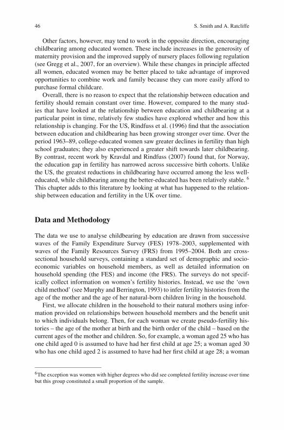
46 S. Smith and A. Ratcliffe
Other factors, however, may tend to work in the opposite direction, encouragingchildbearing among educated women. These include increases in the generosity ofmaternity provision and the improved supply of nursery places following regulation(see Gregg et al., 2007, for an overview). While these changes in principle affectedall women, educated women may be better placed to take advantage of improvedopportunities to combine work and family because they can more easily afford topurchase formal childcare.
Overall, there is no reason to expect that the relationship between education andfertility should remain constant over time. However, compared to the many stud-ies that have looked at the relationship between education and childbearing at aparticular point in time, relatively few studies have explored whether and how thisrelationship is changing. For the US, Rindfuss et al. (1996) find that the associationbetween education and childbearing has been growing stronger over time. Over theperiod 1963–89, college-educated women saw greater declines in fertility than highschool graduates; they also experienced a greater shift towards later childbearing.By contrast, recent work by Kravdal and Rindfuss (2007) found that, for Norway,the education gap in fertility has narrowed across successive birth cohorts. Unlikethe US, the greatest reductions in childbearing have occurred among the less well-educated, while childbearing among the better-educated has been relatively stable. 6
This chapter adds to this literature by looking at what has happened to the relation-ship between education and fertility in the UK over time.
Data and Methodology
The data we use to analyse childbearing by education are drawn from successivewaves of the Family Expenditure Survey (FES) 1978–2003, supplemented withwaves of the Family Resources Survey (FRS) from 1995–2004. Both are cross-sectional household surveys, containing a standard set of demographic and socio-economic variables on household members, as well as detailed information onhousehold spending (the FES) and income (the FRS). The surveys do not specif-ically collect information on women’s fertility histories. Instead, we use the ‘ownchild method’ (see Murphy and Berrington, 1993) to infer fertility histories from theage of the mother and the age of her natural-born children living in the household.
First, we allocate children in the household to their natural mothers using infor-mation provided on relationships between household members and the benefit unitto which individuals belong. Then, for each woman we create pseudo-fertility his-tories – the age of the mother at birth and the birth order of the child – based on thecurrent ages of the mother and children. So, for example, a woman aged 25 who hasone child aged 0 is assumed to have had her first child at age 25; a woman aged 30who has one child aged 2 is assumed to have had her first child at age 28; a woman
6The exception was women with higher degrees who did see completed fertility increase over timebut this group constituted a small proportion of the sample.
3 Women’s Education and Childbearing: A Growing Divide 47
aged 35 who has one child aged 10 and another aged 8 is assumed to have had herfirst birth at age 25 and her second birth at age 27, and so on. As these examplesillustrate, we combine ‘current’ birth probabilities (i.e. whether or not a woman hasa birth in the year in which she is observed in the FES/FRS sample) with retrospec-tive birth probabilities (i.e. whether she had a birth in previous years based on theages of her children). Finally, we use survival analysis to construct cohort parityprogression ratios from the individual fertility histories.
Clearly, the own child method is not without its potential problems. One is thatwe observe the current ages of the mother and any children, but not their actual datesof birth. In practice, a woman aged 25 who has one child aged 0 may actually havegiven birth when she was 24. Since the woman could not be a year older than wecurrently observe her to be when she gave birth, our estimates of the proportion ofwomen who have births of order b by a particular age, and the average age at birthorder b, will tend to have a systematic downward bias. However, the bias shouldapply equally to all cohorts and education groups, and should not therefore affectthe validity of the inferences we draw about differences in fertility behaviour overtime and by education.
A second problem is that the own child method relies on information on survivingchildren in the household to infer fertility histories – infant mortality and householdreconstitution will result in measurement error. However, low rates of child mortal-ity7 and the fact that the overwhelming majority of children stay with their naturalmother in the event of family break-up act to reduce the effect of these factors inpractice.
Another potential problem – one that is more serious in practice – is that olderwomen may have had children who have now left home. If we observe a womanaged 39 with no children, we cannot say for certain whether she has not yet hadchildren, or she had one child when she was 17 who left home when they were 20.8
In the latter case, the own child method would fail to capture births to women whohad children relatively young – we would tend to over-estimate the mean and medianages associated with different birth orders (i.e. the average ages of the mother atfirst, second and subsequent births) and to under-estimate family size for peoplewho entered childbearing at a relatively young age.
A solution to this problem is to adopt a maximum age threshold, i.e. to excludefrom our analysis women above a threshold age at which the problem of childrenleaving home starts to significantly affect the estimates of the proportion of womenhaving births at younger ages. Assuming that women start having children from age16, the selection problems may arise from as young as age 32. In fact, sensitivity
7There was a decline in infant mortality over the period. The rate of death in England and Wales ofchildren less than one year was 14.3 per 1,000 live births in 1976, falling to 5.0 per 1,000 live birthsin 2006 ”Infant and perinatal mortality 2006: health areas, England and Wales”, Health StatisticsQuarterly 35. Our estimates will therefore tend to underestimate births more at the beginning ofthe period.8The problem is made potentially worse in practice by the fact that students who live away fromhome are not counted as part of the household in the FES/FRS.

48 S. Smith and A. Ratcliffe
analysis of estimates of the proportion of women having a first birth by age 20 madeusing successively older samples, shows that the threshold can be raised to 37 beforethere are significant effects.9
Our analysis of fertility therefore excludes births after age 38. This means thatwe under-estimate the proportion of each cohort having first and subsequent births.Murphy and Grundy (2003) suggest that fewer than 1% of births are to women aged40+ among cohorts born after 1930. However, the recent trend towards later child-bearing suggests that the bias is likely to increase among later cohorts. Moreover,the effect of the bias will not be the same across education groups. This must beborne in mind when interpreting our results and we place more emphasis on ouranalysis of the age at first birth rather than completed fertility.
The advantages of generating cohort fertility profiles by applying the own childmethod to repeated cross-section data from the FES and FRS are that we havefull information on birth order, which is only recently available in complete formin data derived from official birth registration data. We also have information onthe mother’s education, as well as other economic and demographic characteristicswhich we use to document changes in employment and partnership among womenwith different levels of education.
As a check of the validity of our approach, we compare an estimate of the periodtotal fertility derived from the FES/FRS data from 1968 onwards, with the officialmeasure of total fertility derived from registration data, shown over a longer periodto highlight fertility trends. Total fertility measures the number of children a womanwould have if she experienced the age-specific fertility rates in that year. As shownin Fig. 3.3, total fertility estimated using the FES/FRS is very close to the officialmeasure. As is to be expected, our estimate is lower than the official measure sincewe exclude births over 37. However, we pick up the major trends in fertility (in par-ticular, the decline in total fertility from around 2.5 in 1968 to 1.7 by the end of theperiod), and the average difference is relatively stable over time.
3.5
3
2.5
2
1.5
1
0.5
Tota
l fer
tilit
y ra
te
Year1930 1940 1950 1960 1970 1980 1990 2000
ONS FES/FRS
Fig. 3.3 Total fertility –FES/FRS estimate and ONSestimate(Social Trends 30 and SeriesFM1 No.35)
9This suggests that there may be a negative relation between the age of the mother at first birth andthe age at which the child leaves home.

3 Women’s Education and Childbearing: A Growing Divide 49
Changes in Childbearing by Education
Rendall and Smallwood (2003) looked at differences in childbearing in women bornin 1954–58, between those with and without post-secondary-school qualifications.We extend the analysis to consider women born in earlier and later cohorts in orderto assess the extent to which the education gap has changed over time. We focus onwomen born ten years’ earlier (i.e. 1944–48) and ten years’ later (i.e. 1964–68).
Information on academic qualifications is not available in all waves of the FESand FRS. Instead, there is consistent information available since 1978 on the age atwhich people leave full-time education. Replicating the exact split made by Rendalland Smallwood is therefore not possible. Instead, we define two groups of edu-cated women – one who left full-time education at 19+ (we call these women withhigher qualifications) and the other who left full-time education at 21+ (we callthese graduate women). In both cases, we compare their outcomes with those ofwomen who left school at 16 or below (we call these school leavers). Rendall andSmallwood report that 17% of their sample had obtained a higher qualification; thefigures reported in Table 3.3 below suggest that this corresponds closely to the pro-portion leaving full-time education at age 19+. However, compared to Rendall andSmallwood, our sample may differ in that we may miss some women who obtainedacademic qualifications after they left full-time education, and not take account ofwomen who stayed on in full-time education but did not obtain any qualifications.
Table 3.3 presents two sets of summary statistics on childbearing by cohort andeducation – completed fertility and the proportion remaining childless. In bothcases, as already discussed, we only include women up to age 38. Rendall andSmallwood do not calculate completed fertility by education, but we can com-pare our estimates of childlessness with theirs for the 1954–58 cohort. For womenleaving school at 16 (corresponding to their sample of women with no educational
Table 3.3 Summary measures of childbearing, by cohort and education
1944–48 1954–58 1964–68
Completed fertility up to age 38
Left school at 16 1.97 1.93 1.94Left FT education at 19+ 1.58 1.45 1.40Left FT education at 21+ 1.55 1.42 1.36
Proportion childless up to age 38
Left school at 16 0.125 0.144 0.149Left FT education at 19+ 0.244 0.290 0.310Left FT education at 21+ 0.272 0.296 0.326
Proportion of cohort
Left FT education at 19+ 0.117 0.174 0.212Left FT education at 21+ 0.090 0.131 0.150
Source: Authors’ calculations using data from the Family ExpenditureSurvey and Family Resources Survey, 1978–2005.

50 S. Smith and A. Ratcliffe
qualifications), we find that 14% are childless, compared to 15% in the LongitudinalStudy. For women with higher qualifications, however, our estimate of childlessnessis quite a bit higher – nearly 30% compared to 22.5% in the Longitudinal Study. Ofcourse, births after the age of 38 may account for the difference. We obtain a muchcloser match when we look at the proportions having a first birth at different ages.In the Longitudinal Study, 10% of women with higher qualifications had their firstbirth by age 24 compared to 50% of women without. We obtain figures of 10% and53% respectively.
The figures in Table 3.3 illustrate that the divide in childbearing by educationappears to have been getting wider. Better-educated women in the 1944–48 cohorthad lower completed fertility and a higher level of childlessness than those wholeft school at 16. By the 1964–68 cohort this gap had widened. Completed fer-tility fell by more among the group with higher qualifications than among thosewho left school at 16 and the gap in completed fertility between the two groupsincreased from 0.42 to 0.58. Of course, we cannot rule out that higher fertility atlater ages among educated women may be enough to maintain levels of childbear-ing but other studies based on the UK cohort studies also point to increasing levelsof childlessness among educated women (see Kneale and Joshi, 2007). The Tablesuggests that most of the increase in the gap occurred between the 1944–48 cohort
1944–48 1954–58 1964–68 1974–78
0.5
0.4
0.3
0.2
0.1
0
Pro
po
rtio
n o
f w
om
en
Age<20 20–24 25–29 30–34 35+
Left school at 16
0.5
0.4
0.3
0.2
0.1
0
Pro
po
rtio
n o
f w
om
en
Age
<20 20–24 25–29 30–34 35+
Left full-time education at 21+
Fig. 3.4 Age at first birth, bycohort and education(Source: Authors’calculations using data fromthe Family ExpenditureSurvey and Family ResourcesSurvey 1978–2005)

3 Women’s Education and Childbearing: A Growing Divide 51
and the 1954–58 cohort; changes between the later cohorts appear to have beensmaller.
The increased divide between education groups is clear if we look at changes inthe timing of first birth – shown for different date-of-birth cohorts in Fig. 3.4. Forwomen leaving school at age 16, there has been a decline in the size of the peak atages 20–24, indicating a slight increase in the age at first birth. However, the peakhas remained at 20–24 and there has been very little increase in the proportion ofwomen having their first birth in their late 20s or 30s. There has been an increase inthe proportion of women leaving school at 16 who are teenage mothers, particularlyamong the most recent cohort of women (born 1974–78).
By contrast, there has been a clear rightward shift in the distribution of age atfirst birth among graduates. Even among the oldest cohort, childbearing began laterthan among women leaving school at 16, but the most common age of entry intomotherhood for graduates was 25–29 and most had their first child before age 30.By the 1964–68 cohort, this was no longer the case with the peak shifting to 30–34.Early evidence from the 1974–78 cohort however, shows less evidence of a furtherbig shift in the age distribution.
The result is a greater polarization in age of childbearing by education. This isclearly illustrated in Fig. 3.5 which shows, for the 1944–48 and 1964–68 cohorts,the proportion of women having a first birth before 30 according to the age at which
0.80.70.60.50.40.30.20.1
0
0.80.70.60.50.40.30.20.1
0
Pro
po
rtio
n o
f w
om
en
Age completed full-time education16 17 18 19 20
Cohort born 1944–48
21
Proportion of cohort First birth before 30
Pro
po
rtio
n o
f w
om
en
Age completed full-time education16 17 18 19 20
Cohort born 1964–68
21
Fig. 3.5 Proportion with firstbirth by age 30, by cohort andeducation(Source: Authors’calculations using data fromthe Family ExpenditureSurvey and Family ResourcesSurvey 1978–2005)
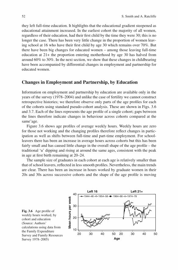
52 S. Smith and A. Ratcliffe
they left full-time education. It highlights that the educational gradient steepened aseducational attainment increased. In the earliest cohort the majority of all women,regardless of their education, had their first child by the time they were 30; this is nolonger the case. There has been very little change in the proportion of women leav-ing school at 16 who have their first child by age 30 which remains over 70%. Butthere have been big changes for educated women – among those leaving full-timeeducation at 21+ the proportion entering motherhood by age 30 has halved fromaround 60% to 30%. In the next section, we show that these changes in childbearinghave been accompanied by differential changes in employment and partnership foreducated women.
Changes in Employment and Partnership, by Education
Information on employment and partnership by education are available only in theyears of the survey (1978–2004) and unlike the case of fertility we cannot constructretrospective histories; we therefore observe only parts of the age profiles for eachof the cohorts using standard pseudo-cohort analysis. These are shown in Figs. 3.6and 3.7. Each of the lines represents the age profile of a single cohort; gaps betweenthe lines therefore indicate changes in behaviour across cohorts compared at thesame˜age.
Figure 3.6 shows age profiles of average weekly hours. Weekly hours are zerofor those not working and the changing profiles therefore reflect changes in partic-ipation as well as shifts between full-time and part-time employment. For school-leavers there has been an increase in average hours across cohorts but this has beenfairly small and has caused little change in the overall shape of the age profile – thetraditional ‘u’ dipping and rising at around the same ages, consistent with the peakin age at first birth remaining at 20–24.
The sample size of graduates in each cohort at each age is relatively smaller thanthat of school leavers, reflected in less smooth profiles. Nevertheless, the main trendsare clear. There has been an increase in hours worked by graduate women in their20s and 30s across successive cohorts and the shape of the age profile is moving
1964–681944–48 1974–781954–5840
30
20
10
Mea
n h
ou
rs p
er w
eek
Age
20 30 40 50 20 30 40 50
Left 16 Left 21+
Fig. 3.6 Age profile ofweekly hours worked, bycohort and education(Source: Authors’calculations using data fromthe Family ExpenditureSurvey and Family ResourcesSurvey 1978–2005)

3 Women’s Education and Childbearing: A Growing Divide 53
0.8
0.6
0.4
0.2
0P
rop
ort
ion
wo
rkin
g
<30 hours 30+ hours
1964–681954–581944–48
Left 16 Left 21+ Left 16 Left 21+ Left 16
Youngest child <5
Left 21+
Fig. 3.7 Employment amongwomen with pre-schoolchildren, by cohort andeducation(Source: Authors’calculations using data fromthe Family ExpenditureSurvey and Family ResourcesSurvey 1978–2005)
away from the traditional ‘u’, in part reflecting an increasing dispersion of age ofentry into motherhood. There have also been changes in employment before andafter childbearing. First, there has been a prolonged period of full-time employmentprior to childbearing with very little decline in average weekly hours before age 30for both the 1964–68 cohort and the 1974–78 cohort. Second, there has also been anaccelerated return to work after childbearing. Using data from the UK birth cohorts,Joshi (2002) reports that the median return to work time for graduate mothers fellfrom five years in the 1970s to less than one year in the 1990s. For women with noqualifications the median return to work time remained at five and a half years. Theresult is an increase in employment among women with young children, particularlyamong graduates. This is shown in Fig. 3.7.
Between the 1944–48 cohort and the 1964–68 cohort, the rate of employmentof graduate women with pre-school children increased from 40% to 60% andalmost all of the increase was from a rise in full-time employment (>30 hours).For women who left school at 16, the increase in the rate of employment was
1964–68
1944–48
1974–78
1954–58
1
0.5
0
Pro
po
rtio
n in
a c
ou
ple
Age
20 30 40 50 20 30 40 50
Left 16 Left 21+
Fig. 3.8 Age profile of partnership, by cohort and education(Source: Authors’ calculations using data from the Family Expenditure Survey and FamilyResources Survey 1978–2005)

54 S. Smith and A. Ratcliffe
smaller (from 26% to 43%) and was driven by rises in both part-time and full-time employment. By the 1964–68 cohort, part-time employment rates amongschool leavers had caught up with those of graduate mothers but the full-timeemployment rate was still much lower. This is consistent with the pattern ofchildcare use among the two groups with educated women making more useof formal paid childcare which is more likely to be available on a full-timebasis.
Among graduate women the biggest increase in full-time employment occurredbetween the 1944–48 and 1954–58 cohort, most likely reflecting the introductionof maternity leave in 1975 which benefited the later cohort. This has allowed morewomen to combine employment and children as shown by the increase in full-timeemployment among women with pre-school children (shown in Fig. 3.7). It mayalso explain the move towards “career” jobs since maternity leave allows womento combine work and family, enabling them to reap some of the benefits of earlyinvestment in a career.
Trends in partnership have also differed by education. For graduate women, therehas been a trend towards delayed partnership formation (here partnership includesboth formal marriage and cohabitation) but the eventual rate of partnership amonggraduate women in their mid-30s has remained fairly stable at around 80%. Forwomen leaving school at age 16, the story is quite different. Not only are part-nership rates lower at younger ages, but they have shifted downwards at all ageswith each successive cohort. The rate of partnership at age 35 has fallen from 85%among the 1954–58 cohort to below 70% among the 1964–68 cohort. There hasbeen a correspondingly greater increase in lone-motherhood among this group.Among graduate women with pre-school children, the proportion who are lonemothers increased from 2% among the 1944–48 cohort to 5% among the 1964–68 cohort. Among those leaving school at 16, the increase was from 6% to 22%(Fig. 3.9).
1954
–58
1944
–48
1964
–68
1954
–58
0.4
0.3
0.2
0.1
0
Pro
po
rtio
n w
ho
are
a lo
ne
mo
ther
Left 16 Left 21+
1944
–48
1964
–68
Youngest child <5 Youngest child 5–10
Fig. 3.9 Lone-motherhood,by cohort and education(Source: Authors’calculations using data fromthe Family ExpenditureSurvey and Family ResourcesSurvey 1978–2005)
3 Women’s Education and Childbearing: A Growing Divide 55
Conclusions and Discussion
By comparing childbearing, employment and partnership across successive date ofbirth cohorts, this chapter has highlighted the increased polarisation between thefamily and working lives of women with different levels of education.
Across cohorts of women born in 1944–48, 1954–58 and 1964–68, the patternof childbearing and employment for women leaving school at 16 has remainedrelatively stable. There has been little change in the age at which they begin child-bearing; around half have their first child by age 25 and more than three-quartersby age 30. There has been an increase in employment among those with children,but part-time work remains the norm. The biggest change has been in partner-ship, with an increasing proportion of lone mothers. This reflects both increas-ing rates of divorce and separation and a rise in the number of never-marriedmothers.
Graduate women have experienced much greater changes in childbearing andemployment. Childbearing is increasingly delayed and fewer than 30% now havetheir first birth before age 30. There has been a greater increase in full-time employ-ment – both before and after employment. Partnership has been delayed but whilstthe eventual rate of partnership remains much the same, the rise in lone-motherhoodhas been smaller. Childbearing and partnership are put on hold as more graduatewomen pursue careers but more (if not the majority) now combine careers withmotherhood.
Thus increasing levels of educational attainment across successive generationsof women can account for some – but not all – of the observed changes over time inwomen’s family and working lives. The lives of graduate women themselves havealso changed compared to the lives of earlier cohorts of graduate women. Predictingwhat will happen in the future to women’s childbearing and employment there-fore involves more than just observing changes in educational attainment, but alsounderstanding the evolving family and working lives of women at different educa-tion levels. For later cohorts (born 1974–78) the evidence presented here points toless dramatic shifts in behaviour among graduate women. Figure 3.4 shows similarrates of childbearing by age 30 to the earlier cohort, while Table 3.4 shows that ratesof employment among graduate women with pre-school children have not continuedto increase at such a fast rate. This may indicate that, while there is now a greaterdivide, it is less likely to widen further.
The increased polarisation is likely to have hugely important effects for the livesof the women involved and for their children. The fact that women of differenteducation backgrounds no longer share recognisably the same family and workinglives is seen by some as marking the end of a common sisterhood (Wolf, 2006).
For children, the changes in work and family lives mean a greater material advan-tage for those born to educated mothers. Table 3.4 summarises information onmaternal employment, lone-motherhood and household income for pre-school chil-dren (<5) by mother’s education and year. Unlike previous analysis, which com-pared women of different date-of-birth cohorts whose children would have been

56 S. Smith and A. Ratcliffe
Table 3.4 Women with pre-school children, by education and year
Proportion working30+ hours
Proportion working< 30 hours
Proportion whoare lone mothers
Mean real weeklyincome
16 21+ 16 21+ 16 21+ 16 21+
1978–82 .048 .063 .198 .272 .084 .026 £55 £791983–87 .075 .143 .221 .333 .124 .023 £73 £1211988–92 .095 .242 .253 .295 .183 .037 £87 £1811993–97 .114 .304 .282 .312 .254 .065 £115 £2101998–02 .137 .315 .318 .317 .282 .069 £139 £231
Source: Authors’ calculations using data from the Family Expenditure Survey and FamilyResources Survey 1978–2005.Income is household disposable income in constant 2003 prices.
born at different points in time because of differences in childbearing ages, thisdirectly compares children of the same age at the same point in time.
Of course, the picture from looking at trends in employment and lone-motherhood over time is much the same as looking across cohorts. However, thefinal column shows a measure of household income. The aim is to look at what hashappened over time to family material well-being for children born to women withdifferent levels of education. Reflecting the changes to age at first birth, maternalemployment and partnership, there has been an increasing divide between house-hold incomes, by education. At the beginning of the period (1978–82) the ratioof household incomes of female graduates to school leavers was 1.43. Ten yearslater, this had grown to over 2. More recently, the gap has narrowed back to 1.66,likely as a result of large increases in child-contingent benefits targeted mainly atlow-income households. Between 1999 and 2003, government spending per childincreased by 50% in real terms, a change that was unprecedented over the previ-ous thirty year period and most of the additional spending was targeted at low-income households. However, even this massive increase in government spendinghas not been enough to counter the effect of changes in employment, childbearingand partnership on relative incomes. Compared to 25 years ago, the income gap haswidened.
Children born to graduate women now live in households with relatively higherincomes in their early childhood. Because of rising levels of full-time employ-ment, however, they are also more likely to spend time in formal childcare atyoung ages. Reductions in inputs of maternal time may offset the positive impactof increases in household income. Predicting how these changes will play out interms of later outcomes depends on the overall effects of both these changes. Thereare extensive literatures which attempt to measure the causal effect of income onchild outcomes (health and educational attainment) and of maternal employment onchild outcomes. Very broadly these literatures suggest that a higher level of per-manent income has a positive effect, particularly at younger ages, although this isrelatively small compared to the effect of family background variables, including

3 Women’s Education and Childbearing: A Growing Divide 57
maternal education (Blow et al., 2005). Maternal employment has generally notbeen found to have a negative effect (Gregg et al., 2005), with some evidence forlong-term positive effects of pre-school formal childcare (Goodman and Sianesi,2005). If anything, therefore, the changes in working and family lives that haveoccurred seem likely to amplify further the advantages for children born to graduatewomen.
References
Becker, G. (1981) A Treatise on the Family, Harvard University Press, Cambridge Mass.Blow, L, Goodman, A, Walker, I. and Windmeijer, F. (2005) Parental Background and Child Out-
comes: How Much Does Money Matter and What Else Matters? Department for Education andSkills Research Report RR660 http://www.dfes.gov.uk/research/data/uploadfiles/RR660.pdf
Cigno, A. (1991) Economics of the Family, Clarendon Press, Oxford.Dex, S, Ward, K. and Joshi, H. (2005) Changes in women’s occupations and occupational mobility
over 25 years, CLS Working Paper, Centre for Longitudinal Studies, London.Ermisch, J. (1989) Purchased childcare, optimal family size and mother’s employment; theory and
econometric analysis, Journal of Population Economics, 2(2): 79–102.Goldin, C. (2006) The quiet revolution that transformed women’s employment, education and fam-
ily, American Economic Review, 96(2): 1–21.Goodman, A. and Sianesi, B. (2005) Early education – how long do the impacts last? Fiscal Studies,
26(4): 513–548.Gregg, P., Burgess, S., Propper, C. and Washbrook, E. (2005) The effects of a mother’s return to
work decision on child development in the UK, The Economic Journal, 115: F4–F80.Gregg, P. Gutierrez-Domenech, M. and Waldfogel, J. (2007) The employment of married mothers
in Great Britain, 1974–2000, Economica, 74(296): 842–864.Gregg, P., Grout, P., Ratcliffe, A., Smith, S. and Windmeijer, F. (2008) How important is pro-social
behaviour for the delivery of public services? CMPO Working Paper, Bristol.Happel, S., Hill, J. and Low, S. (1984) An economic analysis of the timing of childbirth, Population
Studies, 38: 299–311.Hansen, K., Hawkes, D. and Joshi, H. (2009) The timing of motherhood, mothers’ employment
and child outcomes, in Stillwell, J., Coast, E. and Kneale, D. (eds.) Fertility, Living Arrange-ments, Care and Mobility: Understanding Population Trends and Processes Volume 1, SpringerDordrecht, pp. 59–80.
Hoem, J, Neyer, G. and Andersson, G. (2005) Childlessness and educational attainment amongSwedish women born 1955–59, WP-2005–014, Max Planck Institute for DemographicResearch, Rostock.
Joshi, H. (2002) Production, Reproduction and Education: Women, Children and Work in a BritishPerspective, Institute of Education mimeo.
Kaplan, G., Goodman, A. and Walker, I. (2004) Understanding the effects of early motherhood inBritain: the effects on mothers, Discussion Paper No. 1131, Institute for the Study of Labor(IZA).
Kneale, D. and Joshi, H. (2007) Social polarisation in the timing of first birth, Presentation toBritish Society of Population Studies, University of St Andrews, September 12th 2007.
Kravdal, O. and Rindfuss, R. (2007) Education and fertility in Norway – a study of how the rela-tionship has changed over time among women and men, Presentation to GeNet Seminar ‘LowFertility in Industrialised Countries’, London School of Economics, May 31st 2007
Murphy. M. and Berrington, A. (1993) Constructing period parity progression ratios from house-hold survey data, in Ni Bhrolchain, M. (ed.) New Perspectives on Fertility in Britain, Stud-ies on Medical and Population Subjects No. 55, Office of Population Censuses and Surveys,London.

58 S. Smith and A. Ratcliffe
Murphy, M. and Grundy, E. (2003) Mothers with living children and children with living mothers:the role of fertility and mortality in the period 1911–2050, Population Trends, 112: 36–48.
Rendall, M.S. and Smallwood, S. (2003) Higher qualifications, first-birth timings and further child-bearing in England and Wales, Population Trends, 111: 18–26.
Rindfuss, R., Morgan, P. and Offutt, K. (1996) Education and the changing age pattern of Americanfertility, Demography, 33(3): 277–290.
Simpson, R. (2009) Delayed childbearing and childlessness, in Stillwell, J., Coast, E. and Kneale,D. (eds.) Fertility, Living Arrangements, Care and Mobility: Understanding Population Trendsand Processes Volume 1, Springer Dordrecht, pp. 23–40.
Shkolnikov, V., Andreev, E., Houle, R. and Vaupel, J. (2007) The concentration of reproductionin cohorts of women in Europe and the United States, Population and Development Review,33(1): 67–99.
Walker, I. and Zhu, Y. (2003) Education, earnings and productivity: Recent UK evidence, LabourMarket Trends, 111(3): 145–152.
Wolf, A. (2006) Working girls, Prospect Magazine, (April).

Chapter 4The Timing of Motherhood, Mothers’Employment and Child Outcomes
Kirstine Hansen, Denise Hawkes and Heather Joshi
Introduction
The last decades of the twentieth century have witnessed, as part of the seconddemographic transition affecting most industrial countries (Van de Kaa, 1987), twofeatures of particular interest here – a delay in entry to motherhood and an increasedchance of women being employed even after they have children. In Britain, thesetrends have not been experienced uniformly across the social spectrum. The researchreported in this chapter attempts to establish links between these two phenom-ena, to quantify the extent of social differentials (in the timing of first motherhoodand maternal employment) and to investigate their impact on the development ofchildren.
In the not so distant past, very few mothers had paid work, especially duringthe early years of their child’s life. Becoming a mother in your early twenties andstaying at home was the normal course of events and the conventional wisdom atthe time disapproved of anything, such as employment, which might disrupt thebond (or attachment) between mother and her child. However, over the past fiftyyears much has changed. There was a baby boom in the 1950s and 1960s followedby falling fertility rates and rising age at first, and subsequent, births from 1970onwards. By the twenty-first century, mothers working had become the norm. Twothirds (65.4%) of mothers with dependent children were in employment in 2002.Over half (52.9%) of those with a child under five had jobs (Duffield, 2002). Fifty-four per cent of the members of the Millennium Cohort Study had an employedmother when they were three years old (at sweep two, 2003–5) whilst 58% had anemployed mother when they were five years old (at sweep three, 2006). Of thosemothers who were employed at sweep two, 76% were working part-time (Wardand Dex, 2007). However, the increase in maternal employment has not occurred
K. Hansen (B)Centre for Longitudinal Studies, Institute of Education, University of London, London, UKe-mail: [email protected]
J. Stillwell et al. (eds.), Fertility, Living Arrangements, Care and Mobility, UnderstandingPopulation Trends and Processes 1, DOI 10.1007/978-1-4020-9682-2 4,C© Springer Science+Business Media B.V. 2009
59

60 K. Hansen et al.
uniformly across the population. Those who are more likely to be in paid work arealso those who are most likely to have had their children relatively late. Indeed, theage at which a woman enters motherhood has become more spread out in recentyears, with those from the most disadvantaged situations still tending to becomemothers at a young age, and subsequently, being most likely to be out of the labourmarket.
For the families of mothers in employment, a key decision is who takes respon-sibility for their children whilst they are at work. There are social differenceshere too, with those who can afford it purchasing formal childcare from trainedproviders, while for others cost remains a barrier to this type of care. Other parentsput a premium on informal care, attracted by knowing the carer or the flexibilityof making informal arrangements with family and friends. The impact of thesechildcare modes on children is a growing area of research amongst social scien-tists (UK studies include Gregg et al., 2005; Hansen and Hawkes, 2009; Sylva et al.,2004).
Since 1997, the Government has brought in a suite of measures to reduce childpoverty and inequality. The Social Exclusion Unit (SEU) has initiated attemptsto reduce teenage motherhood and to attempt to improve life for the mother aswell as the child (SEU, 1999). Several other policies have attempted to reducechild poverty by increasing the employment of mothers. These include the pro-vision of good quality childcare, local child and family-based initiatives throughthe Sure Start programme, the introduction to the right to ask for flexible work-ing agreements, the extension of maternity leave, the introduction of paternity leaveand, for those who have been out of the labour market for some time, the intro-duction of additional training and job search advice through ‘New Deal for LoneParents’.
This drive towards increasing mothers’ employment, especially when childrenare very young, has led many researchers, as well as the public, to ask about theimpacts on the children. Our research has focused on the consequences of maternalemployment and the timing of motherhood for cognitive and behavioural outcomesin children. Our data resource is the UK birth cohort studies of 1958, 1970 and theMillennium (Bynner and Joshi, 2007). We use these data to illuminate differencesacross families by age at first motherhood, maternal employment, childcare andsubsequent child outcomes.
This chapter therefore presents the results of our project in three key areas: thetiming of motherhood, maternal employment, childcare and the consequences forthe children. We address the following questions:
• What are the main determinants of age at motherhood, and have these changedbetween the cohorts?
• What are the main determinants of maternal employment in a child’s early life?• What are the impacts of the childcare decisions, maternal employment and age
at motherhood on cognitive and behavioural outcomes for children?

4 The Timing of Motherhood, Mother’s Employment and Child Outcomes 61
In the conclusion, we turn to the possible impact of Government policies inthe last ten years on child cognitive and behavioural outcomes by addressing thefollowing questions:
• Will the policies of the last decade help to reverse the increasing polarisation ofage at motherhood and maternal employment that we saw develop in the secondhalf of the 20th century?
• Will this help to reduce the social disadvantage felt by those who grow up insome of the most socially disadvantaged households in the UK?
In undertaking this research, we are adding to an existing literature on the socio-economic variations around the timing of the initiation of childbearing, which it maybe useful to review briefly.
Literature on Timing of Motherhood
Despite a general and international trend towards later motherhood, early child-bearing is still relatively common in the UK compared to other European countries(Chandola et al., 2002). It is also distinctive for its socio-economic covariates(Buxton et al., 2005; Rendall et al., 2008). Less advantaged women still tend tohave children earlier and it is the most advantaged who have increasingly deferredchildbearing (Rendall et al., 2005). This social polarisation in age at motherhood hasemerged in Britain as the trend towards later childbearing in the last three decadesof the century has affected various social groups differentially, and has differentialconsequences.
There are many studies of the socio-economic determinants of the timing ofmotherhood (e.g. Kiernan and Diamond, 1983; Kiernan, 1992, 1997; Ermisch andPevalin, 2003a; Rendall and Smallwood, 2003). In particular, teenage motherhoodis associated with exclusion from both employment and education (Bynner andParsons, 1999; SEU, 1999). Research attempting to disentangle the causes of earlymotherhood and associated problems suggests that early motherhood is a markerrather than a driver of subsequent labour market disadvantages. Work by Ermischand Pevalin (2003b, 2005) on the British birth cohort of 1970 suggests that a teenbirth has little independent effect on a woman’s qualifications, employment or earn-ings at age 30. Work on sisters in the US (Geronimus and Korenman, 1992) andtwins in the UK (Hawkes, 2008) also suggest that early motherhood is stronglyassociated with poor family background. The apparent effects of entering mother-hood early on household income and educational attainment are much smaller onceantecedent factors are taken into account. However Ermisch and Pevalin (2003b,2005) do attribute the lower employment and educational attainment of any partnerpresent when a teen mother reaches 30 to a reduction of prospects in the ‘marriagemarket’. Liao (2003) finds another independent, adverse, effect of early motherhoodon a woman’s mental health.

62 K. Hansen et al.
The timing of motherhood, early or late, may be the outcome of a deliberate strat-egy or it may be unintended, early because of unplanned pregnancy, or late becauseof unplanned infertility (or unanticipated absence of a suitable partner). Probablyeach type of account applies to some individuals. Early motherhood may constitute,for some, a rational choice in the face of limited alternative prospects in educationor employment, along with the safety net of the UK benefit system (Rendall et al.,2008). For others, the main explanation might be a lack of planning and informa-tion (Barrett and Wellings 2002; Allen and Bourke Dowling, 1998; Kneale, 2009).Young mothers may or may not have positively wanted to have a baby at the timethey did, and they may not be consciously aware of the state benefits available.Whatever the explanation for their mothers’ behaviour, any differential outcomesfor families started early and late are certainly not chosen by the children. Whateverits cause, young age at motherhood could be viewed as a signal of disadvantage ona number of fronts, including consequences for the children (Pevalin, 2003).
The implications of these associations are not only present for the mother, butalso for the next generation. As the established British Birth cohort studies of 1958and 1970 have shown (Gregg et al., 1999; Hobcraft and Kiernan, 2001; Feinstein,2003; Blanden et al., 2005; Schoon, 2006), being born into an advantaged or disad-vantaged family may affect the experience of childhood and prospects in later lifefor children. Being born to a mother who had her first child in her teens or earlytwenties is emerging as an increasingly distinctive feature of the intergenerationaltransmission of disadvantage, which at the same time accelerates the cycle.
Timing of Motherhood
Although the post-war era started with rising fertility and falling age of childbearing,the decades since 1970 and the generations of women born since 1940 have beencharacterised by a general postponement of motherhood. Later first birth pushessecond and subsequent births to later ages, although there has also been a downwardtrend in the proportions proceeding to families larger than two. The age by whichhalf of a cohort had embarked on having at least one child reached a low of around23 for cohorts of women born in the 1940s and has been rising ever since to nearly 29for cohorts born in the mid 1970s. These estimates for England and Wales are basedon births up to 2006 and the adjustments made for true birth order (Smallwood,2002; ONS, 2007, Table 10.3).
An alternative indicator is the mean age of women having their first birth in agiven calendar year. This statistic was 27.6 years in 2006 and 25.5 in 1990, as shownin Fig. 4.1. This period measure of age at entry to motherhood is plotted for the years1990–2006 for all birth orders, and first births only, incorporating adjustments fortrue birth order (Smallwood, 2002; ONS, 2007, Table 1.7b). This shows that acrossthose 16 years the age at first birth rose by nearly two years, while the age of mothersat all births rose by 1.4 years. The upward drift of delayed entry to motherhood alsopushes up ages at higher orders.

4 The Timing of Motherhood, Mother’s Employment and Child Outcomes 63
All births First births (true order)30
29
28
27
26
25
24
23
Mea
n a
ge
Year
1990
1991
1992
1993
1994
1995
1996
1997
1998
1999
2000
2001
2002
2003
2004
2005
2006
Fig. 4.1 Mean age at all andfirst births, England andWales, 1990–2006(Source: ONS, 2007;Smallwood, 2002)
Figure 4.2 shows a time series for England and Wales from 1958 until 2004based on the more generally available data on first births within marriage, and allbirths outside marriage, for which birth order is not collected at registration (ONS,2005). We can see that since 1970 for both groups there has been an upward trend inthe age at birth. We can also see that those who had births outside of marriage wereyounger, on average, than those who had first births inside of marriage, despite therise in childbearing within cohabitations boosting the numbers of non-marital birthsin the later years.
Table 4.1 presents the mean age at childbearing in three UK birth cohort studiesand the national registration taken from the ONS (2005) for first births and allbirths. For both series, the age of the cohort child’s mother in the three cohortstudies reflects the general trend found in the national data, with ages starting torise from 1970. Mothers in the Millennium Cohort Study (MCS) were significantlyolder, in terms of both all birth orders and first births only, than those in theNational Child Development Study (NCDS) of 1958 as well as the British CohortStudy (BCS) in 1970. The difference in age at first births is nearly four years (3.8)between 1970 and 2000–1.
The upward trend in the age at first birth has not applied uniformly to the wholedistribution, which is more easily seen by considering cohorts, women themselvesborn in a particular year, rather than as above, all the women giving birth in aparticular year. Figure 4.3 presents the age by which successive quintiles of the
32
30
28
26
24
22
20
Mea
n a
ge
Year
1958
1960
1962
1964
1968
1970
1972
1974
1976
1978
1980
1982
1984
1986
1988
1988
1990
1992
1994
1996
1998
2000
2002
2004
Births outside marriage First births within marriage
Fig. 4.2 Average age at firstbirths within marriage and allbirths outside marriage,England and Wales,1958–2004(Source: ONS, 2005).

64 K. Hansen et al.
Table 4.1 Age of mothers at first and all births, three birth cohort studies and registration statistics
NCDS BCS MCS
Year 1958 1970 2000–1
Mean age of mothershaving first birth
24.4 23.1 26.9
[95% Confidence Interval] [24.3, 24.5] [22.9, 23.2] [26.5, 27.2]Mean age of all mothers at
birth of cohort27.5 26.0 28.9
[95% Confidence Interval] [27.4, 27.5] [25.9, 26.1] [28.7, 29.1]Births of any order
registered in England andWales (ONS, 2005)
27.8 26.2 29.1
Source: Authors’ analysis; ONS (2005).
whole cohort had entered motherhood. This shows that the first 20% of successivecohorts have entered motherhood under or around age 20. The rising age ofmotherhood for cohorts born since 1940 has particularly affected ages over 25 withhalf of the cohort entering motherhood later, if at all. The number of years betweenthe first 20% and the last was 8 years for the 1940 cohort and 18 for the last one wehave a complete fertility history for, those born in 1965. In the 1940 cohort entryto motherhood was relatively compressed into the twenties. Two to three decadeslater it is becoming more spread out, and as we shall see below, more sociallydifferentiated.
We have already seen in Fig. 4.2 that the persistence of young entry to mother-hood is associated with births outside marriage. Another dimension, along whichwomen vary by age at first motherhood, is education. In particular, there is alink between higher education and delayed motherhood. From their analysis ofthe women born in the mid 1950s in the Longitudinal Study (LS) of England andWales, Rendall and Smallwood (2003, p. 25) conclude that women “who obtaineda higher-education qualification began motherhood, on average five years later than
45
40
35
30
25
20
15
Mea
n a
ge
Year
1925
1930
1935
1940
1945
1950
1955
1960
1965
1970
1975
1980
1985
0.8 0.40.6 0.2
Fig. 4.3 Age by whichsuccessive quintiles of thewhole cohort had enteredmotherhood(Source: ONS, 2005)

4 The Timing of Motherhood, Mother’s Employment and Child Outcomes 65
did women who did not obtain a higher qualification”. They also show that the pro-portion of first-time mothers who have a higher qualification is greater at later ages.
As part of this project, Jenkins et al. (2008a) consider the timing of mother-hood for women born in 1958, exploiting the richness of the fertility and employ-ment history data available in the NCDS. As these data are longitudinal and theparticipants in the survey have been followed for over 45 years it is possible toconsider the entry to motherhood for the cohort members themselves in termsof information across their life course to date. Using event history analysis, i.e.looking at the probability of having a birth of a given order, at a given time,for women who had not (yet) had such a birth; Jenkins et al. (2008a) find thestrongest predictor of transition to a first birth is the woman’s education. Thechance of having a first birth is strongly negatively associated with the levelof education, even after controlling for a number of childhood background fac-tors and making allowances for an otherwise unobserved propensity to progressto the next birth. The next birth is defined as births from the second up to thefourth.
Jenkins et al. (2008b) extended their work on the NCDS to consider the timingof motherhood for members of the BCS70 cohort, taking birth orders up to thethird birth and allowing for the possibility of an effect of the aggregate labourmarket on birth decisions. The association of early childbearing and individualswith particularly poor labour market prospects (noted above) led to the hypothesisthat the incentive to avoid early motherhood might be stronger when labour marketprospects were better. The NCDS cohort encountered particularly adverse labourmarkets when they were in their mid-twenties and mid thirties. For BCS70 mem-bers these recessions occurred when they were in their mid teens and early twenties.For the BCS sample, education remained the dominant explanatory variable for thetransition to first birth, but the effect was weaker than for the NCDS sample. For theearlier cohort, women with tertiary education were, all else equal, seven times lesslikely to embark on motherhood at a given time (if they had not already done so)while the comparable estimate for women born in 1970 was 3.6, relative to thosewith no qualifications.
The aggregate unemployment rate showed a significant relationship with thehazard of the first birth only for the BCS70 cohort. The estimate was found to benegative, contrary to expectation, and to earlier results, which pooled both cohorts’birth histories up to 2000 only (Dex et al., 2005). According to the 2008 results,‘bad times’ tend to discourage rather than bring births forward. Further investiga-tion could be made of the possibility that unemployment effects vary within thecohort, or that there were changes in the economic and policy environment in theyears after 2000 that were relevant.
Using data on both men and women in the NCDS and the BCS70, Kneale andJoshi (2008) consider the patterns of postponement and the childlessness acrossthe two cohorts. Once again a major factor in both postponement and childless-ness for women, and also men, was education, with the more educated becom-ing parents later, if at all, than their less educated peers. However, they suggestthat if the 1970 cohort do turn out to have a higher incidence of childlessness

66 K. Hansen et al.
(as predicted), this may be due to the unintended consequences of delaying thedecision rather than an active decision not to have children, given the preferencesfor parenthood expressed by those still childless at 34.
The MCS consists of data on around 19,000 children born across the UK in2000/2001 (Hansen, 2008). Hawkes (2008) and Jayaweera et al. (2005) use data onthe mothers of the cohort members to consider possible determinants of the age atfirst birth. The results of these regressions reflect the patterns in the earlier NCDSand BCS70 cohorts, found by Jenkins et al. (2008a, b), among others, but unlikethe event history approach, the analysis is necessarily confined to women who haveactually become mothers. Hawkes (2008) finds that the age at first child is associatedwith both antecedent and current disadvantage. Once again, the woman’s educationis a strong positive correlate of the age at first birth. In addition to low education,those who enter motherhood earlier are more likely to have experienced disadvan-tage in their own childhood, the separation of their own parents, spent time in careand having an unemployed father at the age of fourteen.
Certain ethnic minority groups (especially Pakistani and Bangladeshi) are asso-ciated with early motherhood. Being born outside the UK is surprisingly found to beassociated with later motherhood for some of this sample (though not to Pakistanisand Bangladeshis). One possible explanation for this positive association of age atmotherhood and immigration is that the migration process itself has disrupted anddelayed family formation. Another is that migration is selective of more enterpris-ing and career-motivated individuals, which may be underlined by the selectivity ofimmigration controls. Finally, higher unemployment, measured locally and nation-ally at the time of conception, is found to be associated with earlier motherhood.This finding reflects those of Dex et al. (2005) on births up to 2000, but not in theupdated data set analysed by Jenkins et al. (2008b).
In summary, we confirm that young motherhood is strongly linked to indicatorsof childhood disadvantage, such as having an unemployed father and experiencingfamily break-up, as well as being associated with the situation in the labour market.However, education plays a key role in the timing of motherhood with those whoinvest in more education delaying their entry to motherhood, not only to extend theirenrolment in post compulsory education, but to pursue careers thereafter. It is likelythat maternal education will also be a key determinant in the labour market attach-ment of a mother, and that the anticipation of a career after childbearing, signalledby the level of qualifications, may play a role in decisions about when childbearingstarts. Therefore in the next section we turn to considering maternal employment.
Maternal Employment
Maternal employment, even in the early years of a child’s life, is now more usualthan not in the UK. Figure 4.4 shows the proportion of mothers working bypartnership status (Duffield, 2002). As shown in Fig. 4.4 by the age of the child,maternal employment appears to be linked to partnership status. Across all of theage groups those mothers who are single are less likely to be in work. This may

4 The Timing of Motherhood, Mother’s Employment and Child Outcomes 67
908070605040302010
0Per
cen
tag
e o
f m
oth
ers
Age of youngest dependent child
<5 5–10 11–15 16–18 All withdependent
children
Couple SingleFig. 4.4 Employment ratesfor partnered and singlewomen by age of youngestdependent child, UK, spring2002, not seasonally adjusted(Source: Duffield, 2002)
reflect the relative ease of combining employment with parenthood when there is asecond parent present, but it may not be a pure effect of partnership status alone. Itis likely to be confounded with the woman’s age, since early childbearing is associ-ated with relatively unstable, if any, partnership, as well as low earning power (seeFig. 4.2 and Hawkes et al., 2004). Thus, children who have a young mother are morelikely to have a mother with neither job nor partner. This situation will be linked toa range of disadvantageous experiences for children including a very high risk offamily poverty and a reliance on means-tested benefits which can form a barrier tolabour market entry.
The Birth Cohort Studies can offer a longitudinal perspective on the secularincrease in the employment of mothers of young children. Table 4.2 shows the per-centage of the members of the three Birth Cohort Studies who had an employedmother at some point in the first five years of their life. Although the numbers arenot exactly comparable, they appear to have doubled from 29% in 1958–1963 toaround 58% in 2000–6, with most of the increase occurring before 1970–1975.
Table 4.2 Percentage of mothers in work during time child aged under five years, across threebirth cohorts
NCDS BCS MCS
Employment in first 5 years 29% 48% 58%Base sample of mothers 13,966 11,474 14,396Coverage GB UK
Source: Authors’ analysis.NCDS reports mothers having any paid work before the child went to school. BCS70reports mothers having any paid work at up to the age 5 interview who held a job whichstarted more than a year earlier. MCS reports current employment at age 5 interview.It will include a few who only started after the 5th birthday, but is does not includethose who had worked before age five who were not currently employed. Percentage isweighted.Source: NCDS and BCS rates from Hansen et al. (2006), MCS numbers from Dex andWard (2008).

68 K. Hansen et al.
0.6
0.5
0.4
0.3
0.2
0.1
0Cu
mu
lati
ve %
of
wh
ole
sam
ple
Month<1 1 2 3 4 5 6 7 8 9
Fig. 4.5 Month ofreturn/entry to employmentafter birth(Source: Authors’ analysis)
Figure 4.5 shows the proportion of mothers in the MCS who had entered employ-ment in the nine months after the birth of the cohort member. The steeper gradientbetween three and four months matches with the end of the paid maternity leave atthe time of the study.
Table 4.3 presents some information on the hours of employment the MCSmothers were undertaking in the first nine months of life. The majority wereemployed in part-time jobs with very few undertaking very long hours.
Crosby and Hawkes (2007) consider the determinants of maternal employmentin the first nine months. The main determinants are maternal employment in the yearprior to the birth and maternal education. Those employed the year before the birthare much more likely to be employed by nine months after the birth than those whowere previously out of the labour market. Of course, being in the labour market ayear before the birth is also likely to be related to maternal education. Maternal edu-cation is also directly linked to early employment post birth, with the more educatedbeing more likely to enter employment in the first nine months. Other significantpredictors of non-employment include having no partner, younger (currently under20) and older (currently over 35 or 40) or belonging to an Asian ethnic group.
In this strand of our work we have also made international comparisons withMCS. This research looks for determinants of the timing of employment afterchildbirth and attempts to infer the role of government policy in these decisions.The results suggest that maternal employment, especially in the early years of
Table 4.3 Work schedule for mothers employed when child aged nine months, MCS
Hours Regularity
Part-time 72%Full-time ( 31–39 hours) 23%40+ hours per week 5%Works regular, daytime hours 54%Other pattern 46%Unweighted n 7,954
Percentages are weightedSource: Crosby and Hawkes (2007)

4 The Timing of Motherhood, Mother’s Employment and Child Outcomes 69
a child’s life, can also be linked to the structure of public policies. Crosby andHawkes (2007) examine differences in the UK (MCS) and the US (Early Child-hood Longitudinal Study of Births (ECLS-B)) while Baxter et al. (2006) comparethe UK (MCS) with Australia (Longitudinal Study of Australia Children (LSAC)).While womens’ education and earning power are associated with the chances ofgetting back into the labour market by the end of the first year in all three coun-tries, there are striking contrasts in patterns of entry and re-entry during those earlymonths.
Both international comparisons provide evidence of the role of the benefit systemand maternity leave policies in the timing of employment after child birth. Thenature of means-tested benefits appears to discourage employment for the poten-tially low paid in the UK but not the US. In the UK the drive to reduce child povertymay have had unintended consequences on the incentives of low paid mothers withregard to employment. Maternity leave policies, applying to at least some of thosewho were employed before the birth, appear to encourage returning to employmentafter a birth, by permitting a delay, which is longer in the UK than US. In Australia,many mothers stayed away from their job for most of the 12 month duration oftheir unpaid leave of absence, whereas in the UK, those with maternity leave rightstended to go back to work either at the expiry of paid leave after four months, or afterunpaid job protection ended at seven months. In the US, where mothers experiencea lack of paid maternity leave and a lack of state benefits, most women enteredemployment very soon after birth. Differentials by education are exacerbated in thatit sorts women into either low paid jobs or jobs with better than statutory maternityleave pay. This is the case in the UK.
Other important determinants of maternal employment in the first nine months ofthe child’s life include: being the first born, being a twin/triplet, and low birth weightwhich all tend to postpone mothers’ employment. Lone motherhood predicts laterentry into post-birth employment for UK (but not US) mothers.
In summary, we find that the maternal employment is strongly linked to themother’s characteristics especially her education. International comparison betweenthe UK and the US/Australia suggest that employment after child birth is also con-ditioned by the benefit system and maternity leave policies.
Childcare and Child Outcomes
Once a mother has decided to enter employment after childbirth one of the mostimportant decisions she has to make is who shall look after her child whilst she is atwork. Table 4.4 presents evidence of the childcare use in the early years for mothersacross the three cohort studies who worked when the child was under 5. This showsthe growing importance of formal childcare in the pre-school years across the threecohorts.
Table 4.5 presents results from a National Survey of Childcare Use (Bryson et al.,2006). For those under five years much of the childcare is informal. Of this informalprovision, grandparents appear to be undertaking the lion’s share of the task.

70 K. Hansen et al.
Table 4.4 Any source of childcare for working mothers of young children across the three birthcohorts
NCDS BCS70 MCS∗∗
1958–1963 1970–1975 2000–2005(0–4 years) (0–4 years) (0–5 years)
Informal only 73.5 19.9 14.3Formal only 39.0∗ 17.7Both formal and informal 41.1∗ 63.9At least some formal 26.5 81.6Observations 4,144 4,246 12,392
Sources: NCDS and BCS numbers from Hansen et al. (2006); MCS numbers from Hansen et al.(2008, Table 5.5).Informal care includes self provision and care provided by partners, grandparents, other relativesand friends. Formal care includes nanny, childminder, nursery, creche provision. Missing numbersin the columns for NCDS and BCS70 represent the different ways of collecting the data due to thegrowing interest in child care issues.∗ Formal only in BCS70 and the mixed category each reduces to 20% if playgroup only is dis-counted (see Table 4.7b in Hansen et al., 2006).∗∗ The MCS figures are based on all families present in all three sweeps of the MCS, not just thosewith working mothers. They also include nursery school as a form of formal childcare.
Table 4.5 Use of provider types in the last week, by age of child
0–2% 3–4% 5–7%
Early years provision and formal childcareNursery school 2 10 +Nursery class 1 22 +Reception class 0 28 5Day nursery 18 12 +Playgroup or pre-school 9 18 +Childminder 5 5 4Nanny or au pair 1 2 1Babysitter 3 2 3Out-of-school club on-site + 2 13Out-of-school club off-site + 1 4
Informal childcare
My ex-husband/wife/partner 3 4 5The child’s grandparent(s) 29 26 22The child’s older brother/sister 1 1 2Another relative 7 6 5A friend or neighbour 5 6 9
Base: All families Umveighted base 1451 1507 1348
Source: Bryson et al. (2006).
The Department for Children, Schools and the Family (DCSF), formerly theDepartment for Education and Skills (DfES), publishes data on the use of pre-schoolprovisions for those who are three or four years old. Figure 4.6 presents these datagraphically, showing the majority of those aged three to four in England and Wales

4 The Timing of Motherhood, Mother’s Employment and Child Outcomes 71
100
80
60
40
20
0
Per
cen
tag
e o
f ch
ildre
n
YearMaintained nursery and primary schools
Independent schools
Private and voluntary providers
20062002 2003 2004 2005
Fig. 4.6 Percentage ofchildren aged three and fourtaking up early educationplaces by type of earlyeducation provider(Source: Department forEducation and Skills, 2006)
attend a state nursery or primary school (nearly 60% in all years between 2002 and2006), with a minority attending independent schools (5% a year) and the remainderattending other private and voluntary places.
Why are these patterns important? We are concerned with the impact of thesethree decisions (timing of motherhood, maternal employment and childcare choice)on the outcomes for children (cognitive, behavioural and health). This will provideus with an indication of possible externalities for children of the government policiestowards parents. Externalities could be a positive or negative in terms of outcomesfor children. We present here the results of our project which consider the impacton child outcomes (cognitive, behavioural and health) on the timing of motherhood,maternal employment and childcare choices.
Firstly, Verropoulou and Joshi (2008) use the NCDS second generation datato consider the association between pre-school employment for the NCDS cohortmembers on the later outcomes for their children, observed in 1991. They find thatreading is slightly poorer where less educated mothers work in the child’s first yearof life. They find few other interactions with employment, but do detect intergener-ational transmission of behavioural as well as cognitive characteristics. The age atfirst birth has a significant independent association only with one of the four out-comes investigated – the child’s maths score which is lower for children with moth-ers aged 20 or less. As all of the children in this study are the offspring of relativelyyoung mothers, it may be difficult to generalize from these findings. However, in sofar as the associations of mothers’ employment with indicators of child developmentare mixed and minor, they are broadly similar to those estimated for the children ofmothers of all ages in the ALSPAC study (Gregg et al., 2005).
72 K. Hansen et al.
Secondly, Crosby and Hawkes (2008) considered the association betweenemployment in the first nine months of life and child cognitive and behavioural out-comes measured at age three years old. The results using the MCS show that mater-nal employment has a positive association with child cognitive outcomes (measuredusing a vocabulary test and a school readiness measure) and child behaviour. How-ever, it is negatively associated with child health, as measured by the body massindex (BMI). After controlling for the selection process into employment, only theassociation between child health and maternal employment is maintained, albeitweakened. The results suggest that maternal education rather than maternal employ-ment in the UK is the main driver for all four child outcomes. Of course educationalso plays a strong role in the selection process into employment.
In our third study, Hansen and Hawkes (2009) consider the role childcare choicehas on child cognitive and behavioural outcomes using the MCS. This paper findsthat for those in employment, different types of childcare have different impacts onchild cognitive and behavioural outcomes at age three. Formal childcare is foundto have positive associations with school readiness measures compared to othertypes of childcare. This is true particularly for children from disadvantaged back-grounds. Care by grandparents appears to have positive effects on a child’s vocab-ulary development but is also negatively associated with behaviour, largely throughpoorer peer relations.
Finally, we examine mother’s age at first birth; whether and when she took upemployment in the child’s first nine months; what main childcare arrangements weremade at nine months; and measures of child development at age three. These areshown in Table 4.6, for mothers of first-born children in the MCS. Although wehave estimated age at first motherhood for cohort children who were not first-born,we do not have such detailed data on employment and childcare in the first year oftheir eldest sibling’s life. The three indicators of child development are the BrackenSchool Readiness, British Ability Scales (BAS) Naming Vocabulary, and the TotalDifficulties Score of the Strengths and Difficulties Instrument. All indicators appearin terms of standard deviations, and are adjusted for age at interview by inclusionof child’s age in the battery of controls noted in Table 4.6. Bear in mind that theDifficulties Score falls when child behaviour improves.
Taken singly, each of these three factors was significantly associated with betterchild outcomes: older mothers, employment in first nine months and use of formalchildcare. However, the multiple regression model enables us to see how far thesepositive associations are attributable to other things. The mother’s level of quali-fication is a dominant predictor of all the outcomes. Putting all the factors in themodel together moderates the differences attributable to age at first motherhood andmode of childcare, and completely accounts for any differences by time of returnto employment in the first year. Once we allow for other factors, particularly forthe education of their mothers, there are few significant differences between chil-dren whose mothers were employed in their first nine months and those who werenot. Children whose mothers worked and had been in formal group care had higherschool readiness scores and lower vocabulary scores than other children. They alsohad significantly better behaviour ratings than children whose mothers stayed at

4 The Timing of Motherhood, Mother’s Employment and Child Outcomes 73
Tabl
e4.
6C
hild
deve
lopm
ent
atag
eth
ree
anal
ysed
bym
othe
r’s
age,
empl
oym
ent
and
child
care
inth
efir
stye
ar,a
ndot
her
cont
rols
:m
ultip
lere
gres
sion
ofm
othe
rsw
hose
coho
rtch
ildw
asth
eir
first
Scho
olR
eadi
ness
(Bra
cken
)N
amin
gV
ocab
ular
y(B
AS)
Tota
lDif
ficut
ies
Scor
e(S
DQ
)
Coe
ffici
ent
Stan
dard
erro
rC
oeffi
cien
tSt
anda
rder
ror
Coe
ffici
ent
Stan
dard
erro
r
Mot
her’
squ
alifi
catio
ns(b
asel
ine:
noqu
alifi
catio
ns)
NV
QL
evel
10.
200.
07∗∗
∗0.
190.
08∗∗
−0.1
70.
09∗
NV
QL
evel
20.
280.
06∗∗
∗0.
270.
07∗∗
∗−0
.32
0.07
∗∗∗
NV
QL
evel
30.
420.
06∗∗
∗0.
310.
06∗∗
∗−0
.45
0.07
∗∗∗
NV
QL
evel
40.
540.
06∗∗
∗0.
420.
07∗∗
∗−0
.52
0.07
∗∗∗
NV
QL
evel
50.
680.
10∗∗
∗0.
390.
09∗∗
∗−0
.46
0.09
∗∗∗
Ove
rsea
san
dot
her
qual
ifc’
s0.
340.
15∗∗
0.03
0.13
−0.3
10.
15∗∗
Mot
her’
sag
eat
(fir
st)
birt
h(b
asel
ine:
14−1
9)
20−2
40.
140.
06∗∗
0.06
0.05
−0.0
60.
06
25−2
90.
300.
06∗∗
∗0.
230.
05∗∗
∗−0
.22
0.06
∗∗∗
30−3
40.
410.
06∗∗
∗0.
300.
06∗∗
∗−0
.22
0.06
∗∗∗
35−3
90.
350.
08∗∗
∗0.
280.
06∗∗
∗−0
.26
0.07
∗∗∗
40+
0.50
0.22
∗∗0.
240.
15−0
.12
0.15

74 K. Hansen et al.
Tabl
e4.
6(c
ontin
ued)
Scho
olR
eadi
ness
(Bra
cken
)N
amin
gV
ocab
ular
y(B
AS)
Tota
lDif
ficut
ies
Scor
e(S
DQ
)
Coe
ffici
ent
Stan
dard
erro
rC
oeffi
cien
tSt
anda
rder
ror
Coe
ffici
ent
Stan
dard
erro
r
Ret
urne
dto
empl
oym
ent(
base
line:
not
retu
rned
toem
ploy
men
tdur
ing
the
first
nine
mon
ths)
Firs
tthr
eem
onth
s−0
.18
0.11
0.08
0.09
0.20
0.10
∗
Bet
wee
nfo
uran
dsi
xm
onth
s−0
.19
0.11
∗0.
100.
080.
170.
09∗
From
seve
nm
onth
s−0
.12
0.11
0.12
0.09
0.15
0.10
Chi
ldca
rew
hils
tmot
her
empl
oyed
(bas
elin
e:no
tusi
ngch
ildca
re)
Info
rmal
non
grou
p0.
020.
12−0
.22
0.11
∗−0
.30
0.12
∗∗
Fath
er/p
artn
er0.
000.
11−0
.07
0.09
−0.2
30.
11∗∗
Gra
ndpa
rent
0.13
0.11
−0.0
30.
08−0
.15
0.10
Form
alno
ngr
oup
0.08
0.12
−0.1
50.
09−0
.24
0.10
∗∗
Form
algr
oup
0.23
0.11
∗∗−0
.18
0.09
∗∗−0
.29
0.10
∗∗∗
Rsq
uare
d0.
230.
190.
19
Obs
erva
tions
4,64
74,
870
5,10
1
Sour
ce:A
utho
rs’
anal
ysis
.A
llre
gres
sion
sco
ntro
lfo
rth
efo
llow
ing:
Dev
elop
men
tal
cont
rols
:A
geat
asse
ssm
ent,
fem
ale,
low
birt
hw
eigh
t,m
ultip
lebi
rth;
Fam
ilyC
ontr
ols:
Eth
nici
ty,
Eng
lish
only
spok
enat
hom
e,pa
rtne
r,em
ploy
edpa
rtne
r,ho
useh
old
inco
me,
owne
roc
cupi
edho
usin
g,m
othe
r′ sde
pres
sion
atni
nem
onth
s,m
othe
rem
ploy
edfu
lltim
ebe
fore
nine
mon
ths,
regi
on.O
nly
first
born
child
ren
used
inth
isan
alys
is.∗
∗∗1%
∗∗5%
∗10%

4 The Timing of Motherhood, Mother’s Employment and Child Outcomes 75
home, as did those in most other types of childcare except grandparent. Looking atage at motherhood, child outcomes are worst for those who were teenagers at birth(the reference category) and improved as the mothers age rises to some point in thethirties. The improvements reverse somewhat for the small number of mothers hav-ing their first child in their forties. The two cognitive scores peak among mothersaged 30 to 34, and the best behavioural adjustment, other things equal, found amongchildren whose mothers were aged 35 to 39. After these ages the numbers havingfirst births tails off (compare Fig. 4.3). The strength of the association with age atmotherhood can be compared with that of education.
For the school readiness score, the peak difference between having a teenagemother and one whose first birth was at age 30 to 34 (0.41) is equivalent to thedifference between a mother having no qualifications and A levels (NVQ 3). Herea degree is ‘worth’ a premium over no qualifications of 0.54 and a post-graduatequalification – NVQ5 – a premium of 0.68. The child’s vocabulary score is notso strongly related to either education or maternal age, but their 0.30 differentialbetween mothers in the early thirties and teenagers corresponds to the premium forNVQ 3. Among age groups of mothers, those aged 35–39 had children with the bestbehaviour scores, 0.26 below the behaviour problems of the children of teenagers.This can be compared to the indicator with the biggest differential, mothers’ educa-tion. The behaviour scores for children of mothers with NVQ 4 or 5 was 0.52 belowparents with no qualifications. Comparing a mother who had both tertiary qualifica-tions and later entry to motherhood (as most do) with a mother who had her childas a teenager and had no qualifications would involve adding the qualifications andage terms. According to this model therefore, a larger part of the developmentallead observed in the children of older mothers is attributable to their mothers’ edu-cation, but there are more disadvantages to having a very young mother than thoseassociated with her lack of education, or correspondingly, more advantages associ-ated with later motherhood than just those attaching to maternal education. Theseadvantages may be other material, social or psychological ‘capital’ not adequatelycaptured in the model, but they do suggest there could be a gain for the child if itsarrival is delayed until at least well into the twenties.
Conclusions
In this final section, we respond to the three questions asked at the outset:
What are the Main Determinants of the Age at Motherhood,and Have these Changed Between the Cohorts?
Later motherhood in Britain has involved a widening of the span of ages at whichwomen have their first child. This has gone along with widening educational andemployment opportunities for women and increasing childbearing outside marriage.

76 K. Hansen et al.
Education drives fertility beyond those years of post-compulsory enrolmentwhich lead to qualifications but inhibit early fertility. Whether education is enlight-ening or merely a way of signalling better access to the labour market, it can beargued that, by raising the opportunity costs of motherhood it creates an incentiveto defer beyond years of study, if not avoid it. The case for the widening in agesbeing driven by dispersion in educational achievement rather than vice versa can bemade by arguing that women with more human capital, or aspirations to accumulateit, have a greater incentive to defer motherhood than those with poorer educationalor career prospects. Much early motherhood may be unintended, but since fertilitycontrol, including abortion, has become available to those with the motivation andknowledge to use it, it will tend to be those who have least to lose who will becomemothers soonest.
The modelling of the hazard of having a first birth in both the 1958 and 1970cohorts found that a woman’s education was a strong predictor of entering moth-erhood even after allowing for measured (and unmeasured) characteristics andabilities of the women with which it is correlated. However, the strength of thispredictor was weaker in the second cohort, where more women had tertiary educa-tion. In the analysis of the Millennium cohort, whose mothers come from a numberof birth cohorts themselves, we also found poor education and childhood disad-vantage to be predictors of early motherhood, as too was ethnic variation. TheNCDS and MCS studies reach opposite conclusions in the attempt to associate poorlabour market conditions with early births, but perhaps the structure of constraints ischanging.
What are the Main Determinants of Maternal Employmentin a Child’s Early Life?
Here again we find the woman’s education strongly associated with her employ-ment career, both before and in the year after the Millennium cohort child’s birth.Education predicts independently employment in those early months of life andemployment before the birth of the child. Higher employment and higher labourforce attachment are bound up with older motherhood. Over and above the asso-ciation with employment, education and partnership status, the modelling detectedsome further minor differentials by (current) age of mother. International compar-isons helped to reveal how mothers’ employment behaviour in the UK is structuredby state policies. Maternity leave provisions structure the timing of mothers’ returnto work, and the provisions of the means-tested benefits presumably account for thelower rates of employment of lone mothers in the UK than the US, and than part-nered mothers in the UK. An important consideration in the maintaining of careercontinuity after a birth is the arrangements a mother is able to make for childcare.The higher purchasing power of those with high wages and higher qualifications iscrucial in this respect.

4 The Timing of Motherhood, Mother’s Employment and Child Outcomes 77
What are the Impacts of the Childcare Decisions, MaternalEmployment and Age at Motherhood on Cognitive andBehavioural Outcomes for Children?
Until the National Childcare Strategy inaugurated in 1998, most working mothersin the UK used informal childcare before their children reached school age. Themothers of the Millennium Cohort encountered more group nurseries and a greatlyexpanded nursery education provision once their children reached the age of three.During their child’s first year, however, relatively few used formal group day care,and grandparents were an important source of care. Analysis of child outcomes forchildren of the 1958 cohort, assessed in 1991, suggests little impact on the develop-ment of those children in that context. The investigation of evidence emerging on thedevelopment of children born in the Millennium, and assessed at age three (mostlyin 2004), also finds little direct impact of early maternal employment on child out-comes, although there are signs of some types of child care being associated withbetter results on some outcomes. The pattern is nuanced in both the study of thechildren of NCDS members and the results presented here on MCS, it is the verbalscore which has a significant negative association with early employment. The latterdoes not apply if the care arrangement is informal, particularly with a grandparent.It is too early to see how the experience of group childcare and nursery education atages 1 to 4 may be traced in child outcomes. While there seems to be little gained orlost in terms of child development if the mother maintains career continuity, theredoes seem to be a considerable advantage to the child in being born to a motherwith a reasonable level of education as well as one who is closer to age 30 than age20. This confirms the supposition that the intergenerational transmission of socialadvantages is playing out in the most recent cohort to be studied, as well as itspredecessors.
Policy Implications
This research has shown that education is a key correlate of the life course of bothwomen and their children. Whilst maternal age at first birth, maternal employmentand childcare play a role, maternal education appears to be a very strong deter-minant of future success. To what extent it is a fundamental determinant, servingto enlighten and raise skills in production and childrearing; a reflection of capa-bilities inherited from home rather than school; or a signal for social sorting, hasnot been fully established. Whatever lies behind educational attainment it accountsfor much of the difference in outcomes between early and late mothers and in thedevelopment of their children. This also suggests that policies which are successfulin limiting educational failure, such as provision of basic skills and prolonging andsupporting years in education are likely to stem the polarization between early andlate mothers and their children, and have the positive externality of helping the nextgeneration.

78 K. Hansen et al.
The independent association of young age at motherhood with poorer or delayedcognitive and behavioural scores at age three may just reflect unmeasured disad-vantaged antecedents of the minority of women who become mothers in their teensand early twenties. However, the very fact of their youth, perhaps through a lack ofmaturity and of unmeasured current economic and social resources, may compoundthe disadvantages facing their children. If so, government policies to reduce unin-tended teenage motherhood should, if successful, improve the prospects for both thewomen and children involved.
To the extent that early motherhood has its own costs, avoiding it would be anadvisable policy for the private individual as well as public intervention, which can,after all, only inform and support private decisions. There is no evidence here to sug-gest that the gains to postponing motherhood continue indefinitely, at least beyondthe early thirties.
We find little evidence for maternal employment in the first year systematicallyeither harming or promoting child development. We find formal childcare havingboth positive and negative associations with different aspects of child development.This suggests that policies making childcare available to mothers across the spec-trum are likely to be beneficial to both mothers and children, but that attention needsto be paid to its quality. The development of integrated childcare centres under theSure Start programme and other childcare policies aimed at improving the quality ofchildcare received may help have positive spillover effects on some child outcomesand contribute to reversing the polarity between advantaged and disadvantaged fam-ily backgrounds.
References
Allen, I. and Bourke Dowling, S. (1998) Teenage Mothers: Decisions and Outcomes, Policy Stud-ies Institute, London.
Barrett, G. and Wellings, K. (2002) What is a ‘planned’ pregnancy? Empirical data from a Britishstudy, Social Science & Medicine, 55(4): 545–557.
Baxter, J., Joshi, H., Sanson, A. and Ward, K. (2006) Mother’s employment and mental health inthe first year of a child’s life: A contrast between two maternity leave regimes, Presentation atthe International Conference on Child Cohorts, Oxford.
Blanden, J., Goodman, A., Gregg, P. and Machin, S. (2005) Changes in intergenerational mobilityin Britain, in Corak, M. (ed.) Generational Income Mobility in North America and Europe,Cambridge University Press, Cambridge, pp. 112–147.
Bryson, C., Kazimirski, A. and Southwood, H. (2006) Childcare and Early Years Provision:A Study of Parents’ Use, View and Experience, DfES Research Report No 723, National Centrefor Social Research, London.
Buxton, J., Clarke, L. Grundy, E. and Marshall, C.E. (2005) The long shadow of childhood: associ-ations between parental social class and own social class, educational attainment and timing offirst birth; results from the ONS Longitudinal Study, Population Trends, 121(October): 17–26.
Bynner, J. and Joshi, H. (2007) Building the evidence base from longitudinal data: the aims, contentand achievements of the British Birth Cohort Studies, The European Journal of Social ScienceResearch, 20(2): 159–179.
Bynner, J. and Parsons, S. (1999) Young People not in Employment, Education or Training andSocial Exclusion: Analysis of the 1970 Cohort Study, Social Exclusion Unit, London.

4 The Timing of Motherhood, Mother’s Employment and Child Outcomes 79
Chandola, T., Coleman, D.A. and Hiorns R.W. (2002) Distinctive features of age-specific fertilityprofiles in the English-speaking world: common patterns in Australia, Canada, New Zealandand the United States, 1970–98, Population Studies, 53: 317–329.
Crosby, D. and Hawkes, D. (2007) Cross-national research using contemporary birth cohort stud-ies: a look at early maternal employment in the United Kingdom and United States, Interna-tional Journal of Social Research Methodology, Special Issue - Child Cohort Studies, 10(5):379–404.
Crosby, D. and Hawkes, D. (2009) Child outcomes and early maternal employment: evidence forthe UK and the US, submitted to Child Development.
Department for Education and Skills (2006) Provision for Children Under Five Years ofAge in England: January 2006 (Final), This Statistical First Release updates and extendsthe information provided in SFR 17/2006 Provision for Children Under Five Years ofAge in England: www.dfes.gov.uk/rsgateway/DB/SFR/s000674/release.shtml is contained inwww.dfes.gov.uk/rsgateway/DB/SFR/s000674/index.shtml.
Dex, S. and Ward, K. (2008) Parents Employment and Education in Hansen and Joshi (eds) MCS3User Guide to Initial Findings, Centre for Longitudinal Studies, London.
Dex, S., Gustafsson, S., Jenkins, A., Joshi, H., Kenjoh, E., Killingsworth, M.R. (2005) Mothers′
changing labour supply in Britain, the US, and Sweden, in Gomez-Salvador, R. Lamo, A.Petrongolo, B. Ward M. and Wasmer E. (eds.) Labour Supply and Incentives to Work in Europe,Edward Elgar, Cheltenham, UK, pp. 115–150.
Duffield, M. (2002) Trends on Female Employment 2002, Labour Market Trends, 110 (November):605–616.
Ermisch, J., and D. Pevalin. (2003a) Who has a child as a teenager? ISER Working Paper 2003–30,Institute of Social and Economic Research, University of Essex, Colchester.
Ermisch, J., and Pevalin, D. (2003b) Does a teen birth have longer-term impact on the mother?Evidence for the 1970 British Cohort Study, ISER Working Paper 2003–28, Institute of Socialand Economic Research, University of Essex, Colchester.
Ermisch, J.F. and Pevalin D.J. (2005) Early motherhood and later partnerships, Journal of Popula-tion Economics, 18: 469–489.
Feinstein, L. (2003) Inequality in the early cognitive development of British children in the 1970Cohort, Economica, 70 (277): 73–97.
Geronimus, A. and Korenman, S. (1992) The socioeconomic consequences of teen childbearingreconsidered, Quarterly Journal of Economics, 107: 1187–1214.
Gregg, P., Harkness, S. and Machin, S. (1999) Child Development and Family Income, JosephRowntree Foundation, York.
Gregg, P., Washbrook, E., Propper, C. and Burgess, S. (2005) The effects of a mother’sreturn to work decision on child development in the UK, The Economic Journal, 115(501):F49–F80.
Hansen, K. (2008) Millennium Cohort Study. A Guide to the Datasets, Centre for LongitudinalStudies, Institute of Education, University of London, London.
Hansen, K. and Hawkes, D. (2009) Early childcare and child development, Journal of Social Policy,38(2): 211–239.
Hansen, K., Joshi, H. and Verropoulou, G. (2006) Childcare and mothers’ employment: approach-ing the Millennium, National Institute Economic Review, 195(January): 84–102.
Hawkes, D. (2008) The UK Millennium Cohort Study: the circumstances of early motherhood, inEdwards, R. (ed.) Researching Families and Communities: Social and Generational Change,Routledge, Abingdon, pp. 147–163.
Hawkes, D. (2008) The socio-economic consequences of early child bearing: evidence from asample of UK female twins, submitted to Journal of Population Economics.
Hawkes, D., Joshi, H. and Ward, K. (2004) Unequal entry to motherhood and unequal starts in life:evidence from the first survey of the UK Millennium Cohort, Working Paper 6, CLS CohortStudies, London, www.cls.ioe.ac.uk/core/documents/download.asp?id=299&log˙stat=1
Hobcraft, J., and Kiernan, K.E. (2001) Childhood poverty, early motherhood and adult social exclu-sion, The British Journal of Sociology, 52(3): 495–517.

80 K. Hansen et al.
Jayaweera, H., Joshi, H., McFarlane, A., Hawkes, D. and Butler, N. (2005) Pregnancy and childbirth, in Dex, S. and Joshi, H. (eds.) Children of the 21st Century from Birth to Nine Months.The UK Millennium Cohort Study Series, The Policy Press, Bristol, pp. 109–132.
Jenkins, A., Joshi, H., and Killingsworth, M. (2008a) The relationship between educational attain-ment and the timing of first and higher-order births. An Event History Analysis of the NationalChild Development Study, Unpublished paper presented at European Society of PopulationEconomics (ESPE) conference, June, www.econ.ucl.ac.uk/espe2008/
Jenkins, A., Joshi, H., and Killingsworth, M. (2008b) Educational attainment, labour mar-ket conditions and the timing of first and higher-order births in Britain, UnpublishedPaper Presented at European Association of Labour Economists (EALE) Conference, Sept.www.eale.nl/Conference2008/Programme/PapersC/add72162˙tqMZ5V8zNr.pdf
Kiernan, K.E. (1992) The impact of family disruption in childhood on transitions made in youngadult life, Population Studies, 46: 213–234.
Kiernan, K.E. (1997) Becoming a young parent: a longitudinal study of associated factors, BritishJournal of Sociology, 48: 406–428.
Kiernan. K.E. and Diamond, I. (1983) The age at which childbearing starts -a longitudinal study,Population Studies, 37(3): 363–380.
Kneale, D. (2009) Early parenthood: definition and prediction in two British cohorts, in Stillwell,J., Coast, E. and Kneale, D. (eds.) Fertility, Living Arrangements, Care and Mobility: Under-standing Population Trends and Processes Volume 1, Springer Dordrecht, pp. 81–103.
Kneale, D. and Joshi, H.E. (2008) Postponement and childlessness – evidence from two Britishcohorts, submitted to Demographic Research.
Liao, T.F. (2003) Mental health, teenage motherhood, and age at first birth among British womenin the 1990s, ISER Working Paper 2003–33, Institute of Social and Economic Research,University of Essex, Colchester.
Office for National Statistics (2005) Dataset PBH41A Taken from Table 1.6 Published in BirthStatistics 1837–1983, Historical series FM1 No 13, and Vol. No’s 27, 28, 29 and 33.
Office for National Statistics (2007) Birth Statistics Series FM1 no. 35 Review of the RegistrarGeneral on Births and Patterns of Family Building in England and Wales, 2006, Office forNational Statistics, Newport.
Pevalin, D.A. (2003) Outcomes in childhood and adulthood by mother’s age at birth: evidence fromthe 1970 British Cohort Study, Working Paper 2003-31, ISER, University of Essex, Colchester.
Rendall, M.S., Couet, C., Lappegard, T., Robert-Bobee, I., Ronsen, M. and Smallwood, S. (2005)First birth by age and education in Britain, France and Norway, Population Trends, 121: 27–34.
Rendall, M.S., Joshi, H., Lynch, K., Ekert-Jaffe, O. and Mougin, R. (2008) Universal versus eco-nomically polarized change in age at first birth: a French-British comparison, Rand CorporationWorking Paper WR568, http://www.rand.org/pubs/working papers/WR568.
Rendall, M. and Smallwood, S. (2003) Higher qualifications, first-birth timing, and further child-bearing in England and Wales, Population Trends, 111: 18–26.
Schoon, I. (2006) Risk and Resilience: Adaptations to Changing Times, Cambridge UniversityPress, Cambridge.
Smallwood, S. (2002) New estimates of trends in births by birth order in England and Wales,Population Trends, 108: 32–41.
Social Exclusion Unit (SEU) (1999) Teenage Pregnancy, TSO, London.Sylva, K., Melhuish, E., Sammons, P., Siraj-Blatchford, I. and Taggart, B. (2004) The Effective
Provision of Pre-school Education (EPPE) project, Technical Paper 12 – The Final Report,DfES/Institute of Education, University of London, London.
Van de Kaa, D. (1987) Europe’s second demographic transition, Population Bulletin, WashingtonDC.
Verropoulou, G. and Joshi, H. (2008) Does mothers’ employment conflict with child develop-ment? Multi-level analysis of British mothers born in 1958, submitted to Journal of PopulationEconomics.
Ward, K. and Dex, S. (2007) Parental employment, in Hansen, K. and Joshi, H. (eds.) The Millen-nium Cohort Study Second Survey: A User’s Guide to Initial Findings, Centre for LongitudinalStudies, London.

Chapter 5Early Parenthood: Definition and Predictionin Two British Cohorts
Dylan Kneale
Background
Since the baby boom of the 1960s, births in the United Kingdom (UK) have beenfalling in number while age at first birth has risen. Low and late fertility is an impor-tant part of the second demographic transition (Van de Kaa, 1987). In the first yearsof the new millennium, while the total fertility rate has fluctuated slightly and hasonce again begun to rise, or catch up, the tendency to postpone entry to motherhoodhas persisted with a continued rise in average age at first birth (Office for NationalStatistics, 2007). However, this rise has not occurred as a neutral shift towards olderages. While teenage fertility rates have only dropped slightly since peaking in thelate 1990s, this pace of change has not matched the dramatic rise in fertility amongolder age groups (Office for National Statistics, 2007). In 1996, the age-specificbirth rate for teenagers stood at 29.7 per 1,000 women, dropping to 26.6 in 2006.1
In the same period, the rate increased from 37.5 to 53.8 births per 1,000 womenaged 35–39 years. A picture of decreasing fertility in the twenties is painted whenwe recognise that by the age of 30 years, 67% of women born in 1960 would havebecome mothers while for women born just fifteen years later, in 1975, this estimatehad dropped by 10 to 57% (Office for National Statistics, 2007).
Such decreases are usually attributed to postponement, as opposed to large-scaleavoidance of parenthood (Kneale and Joshi, 2008). Put in succinct terms, this almostdenotes “a move towards older fertility for the majority and early fertility for theminority” (Hadfield et al., 2007, p. 255). This unequal shift in the fertility sched-ule is understood to be representative of social polarization in age at first birth(Joshi, 2007, Kneale and Joshi, 2008). Older first-time mothers are associated witha range of advantageous characteristics not shared by early first-time mothers. It is
D. Kneale (B)Centre for Longitudinal Studies, Institute of Education, University of London, London, UKe-mail: [email protected] can be assumed that most teenage births would represent first births. To the author’s knowledge,statistics on birth order for births outside marriage are not collected. We therefore demonstratethese trends using statistics on all births.
J. Stillwell et al. (eds.), Fertility, Living Arrangements, Care and Mobility, UnderstandingPopulation Trends and Processes 1, DOI 10.1007/978-1-4020-9682-2 5,C© Springer Science+Business Media B.V. 2009
81

82 D. Kneale
this polarization in the characteristics and outcomes of first-time mothers –and byextension, fathers and their children – that is the cause of continued concern aboutthe transition into early parenthood.
One of the widespread conventions of the literature on early parenthood is thatparenthood stops being ‘early’ at the age of 20 years. There are various definitionsof ‘teenage’ motherhood in the literature – pregnancy under 16, 18 or 20 – as well asa more literal cut-off of giving birth while still aged 19 or under (Social ExclusionUnit, 1999; Birch, 1996). The concern here is why the line should be drawn at age20. Despite the shift of the fertility schedule, albeit somewhat unbalanced, towardsolder ages, this convenient definition of teenage parenthood remains a pervasiveconcept in studies, with very few extending the cut-off point for early parenthoodbeyond this.2 In studies examining teenage parenthood, there is little or no justifica-tion given as to why the clock stops at 20 years.3 This is despite the fact that manyof our parents and grandparents may have been teenage first-time parents them-selves (Geronimus, 1997). In fact, in her later work, Geronimus describes teenageparenthood as more a political tool than a social construct (Geronimus, 2003), andcertainly, there are grounds to question this distinction. Not only does the age 20threshold come at a convenient point in the coding of ages into five-year bands,but the term ‘teenage’ has other connotations – of adolescence, immaturity and notbeing old enough for the ‘adult’ role of a parent. A ‘teenage parent’ is almost acontradiction in social terms.
In terms of outcomes, there are only a few studies where the distinction ofteenage and early parenthood has been explored. In their study, Hobcraft andKiernan found that the widest gulf in terms of adult outcomes was between thosehaving a first birth under 23 years and those between 23 and 32 years, althoughthis was reinforced by ‘teenage’ parenthood (Hobcraft and Kiernan, 2001). As men-tioned however, studies that experiment with a definition of ‘early’ in terms of out-comes are few and far between. Some researchers who have taken a counterfactualapproach to the timing of parenthood by asking ‘what would have happened had theteenage (mother) delayed childbearing?’ have found no substantial benefit to delay-ing motherhood among this group (Goodman et al., 2004) and have even found earlymotherhood to be a beneficial strategy (Hotz et al., 2004). This again would appearto suggest that joining the labels of teenage and parent in such an unchallengedway is the product of a form of manufactured risk. Throughout this chapter, it is thehypothesis that focus on teenage parents has stemmed from a stigmatised view ofthe ‘correct path to parenthood’ (Hadfield et al., 2007). This focus has seemed dis-proportionate given their low and diminishing prevalence. It is the proposition herethat in terms of predictors, their characteristics do not vary significantly from earlyparents in their twenties.
2The works of Robson and Berthoud (2006) and Hobcraft and Kiernan (2001) provide two exam-ples of a more inclusive definition of ‘early’ parenthood.3This is addressed fully in Kneale (2008).

5 Early Parenthood: Definition and Prediction in Two British Cohorts 83
To examine the validity of the teenage construct, this research uses a number ofdefinitions of ‘early’ through which to examine transition to early parenthood aswell as using different ways of modelling ‘early’. Although this chapter is focusedfirmly on whether age 20 is still a meaningful boundary as concerns the transitionto parenthood, it can also be seen as a contribution to the literature on the timingof ‘youth transitions’ in the life course generally, with many other aspects of adultroles, in the labour and housing markets for example, being ‘delayed’ well beyondage 20 (Pollock, 2008).
Predicting Early Parenthood
The labels ‘early parent’ or ‘teenage parent’ apply to a diverse group of people.Indeed, it has been speculated that the only commonality binding early parents is justthat – that they were young when having children (Harden et al., 2006). However,there is a considerable body of quantitative and qualitative studies finding recurringthemes and patterns that have predictive power over the timing of parenthood. Thesecan be grouped under the following four headings4 and while these groups are notexhaustive, they serve as a useful framework of the factors that are known to besignificant. This framework applies to becoming a parent. It is not within the rangeof this study to examine factors associated with becoming pregnant but avoidingparenthood (abortion) or to examine predictors of avoiding conception (abstinenceand contraception).
Educational Factors
Educational underachievement and cognitive ability have been linked in severalstudies to an increased likelihood of becoming an early parent (Ermisch and Pevalin,2003b; Harden et al., 2006; Jaffee et al., 2001). The pathway often suggested is oneof low qualifications leading to poorer labour market prospects. This in turn lowersthe opportunity costs of having children early (Ermisch and Pevalin, 2003b). Thispathway has applied to the case of early motherhood. For early fatherhood, educa-tional factors are included as a matter of course, although there is little theoreticaldevelopment of such a causal pathway for men as in the case of women. In particu-lar, while low educational achievement is likely to lead to poorer trajectories in thelabour market; there is no theorised substitution of parenthood for career as is thecase for women. A possible pathway that could form from the view that educationmay be important is the partnership market. Low levels of education may, through‘assortative mating’ (or homogamy), go along with a partner with low educationallevel for whom the opportunity cost of early childbearing is low, or who is herself
4References represent only a selected group of studies that examine these predictors.

84 D. Kneale
impatient to start a family. Alternatively, lower educational achievement may beassociated with a greater preponderance to risk taking behaviour which may includefathering early pregnancies.
A limited number of studies have explored the effect of education further throughexamining the effect of disliking school on early pregnancy (Bonell et al., 2005,2007; Imamura et al., 2007; East et al., 2006). In Bonell’s 2005 study, dislikeof school was found to be a potent predictor of early teenage (under 16) preg-nancy and replaced other personal factors. However, this association was statisti-cally accounted for by the inclusion of socioeconomic features (Bonell et al., 2005).In East and colleagues’ study, school orientation was measured as achievement andambition for higher education, both of which were insignificant alongside other fac-tors (East et al., 2006). In qualitative research, links have also been made betweendislike of school and pregnancy, thought to operate along a pathway to reducedopportunity costs in having children early (Arai, 2003). In these data, dislike ofschool has been included in models of entry into parenthood specifically and repre-sents the first such research to do so to the author’s knowledge.
Socioeconomic Factors
Socioeconomic factors have been implicated in a wide range of studies of the pre-dictors of early parenthood and are pervasive in most research, either explicitly or asbackground controls (Bynner et al., 2000, Ermisch and Pevalin, 2003b, Ekert-Jaffeet al., 2002). Usually socioeconomic factors include income, social class and tenure.In this research, while all three spheres are tested to a certain extent, tenure is foundto be the strongest predictor.
All three factors are meant to capture an effect of disadvantage and to predictthe probability of poor labour market success. Schoon and colleagues’ researchprovides a useful framework with socioeconomic background being “one of themain predictors of cognitive development, which provides the underpinnings of aca-demic achievement upon which much success in later life depends” (Schoon et al.,2002, p. 1486). However, the fact that socioeconomic factors retain significanceand sometimes outweigh the effect of educational predictors of early parenthoodsuggests that socioeconomic factors are capturing an element of labour market dis-advantage not completely accounted for by educational factors. Other pathwaysthrough which socioeconomic factors can operate include lowered personal, socialand sexual negotiation skills, limited access to healthcare, lack of positive role mod-els and living in dangerous environments (Singh et al., 2001). In this research,socioeconomic factors are found to be instrumental in distinguishing some defi-nitions of ‘early’ parenthood and are also found to have differential effects betweenmotherhood and fatherhood.
Demographic Factors
An unstable home life is consistently identified as a predictor for the timing of moth-erhood. This can include a history of being in social services care, sexual abuse,parental divorce and parental mental health problems (Kiernan and Hobcraft, 1997).

5 Early Parenthood: Definition and Prediction in Two British Cohorts 85
In this research, against other background controls, an indicator of unstableparental structure (covering divorce, separation, death and foster care) is found tobe a relatively weak predictor of early parenthood. A far more consistent predictoris the age of cohort members’ parents at first birth. This is consistent with otherliterature which finds a cyclical pattern of the timing of motherhood. The SocialExclusion Unit reports that sisters and daughters of teen mothers are six times morelikely to become pregnant at an early age (Social Exclusion Unit, 1999). In theiranalysis of BCS70 data, Ermisch and Pevalin find that women born to teenage oryoung adult mothers (20–23 years old) are around two and a half times more likelyto have a teenage birth themselves (Ermisch and Pevalin, 2003a). This evidence isalso consistent with studies of early fatherhood (Berrington et al., 2005).
Ethnicity is also deemed an important predictor of the timing of motherhood,with non-white women usually at risk of experiencing early births in the UK andUS (Social Exclusion Unit, 1999, Singh et al., 2001; Robson and Berthoud, 2006).Unfortunately in these data, it is not possible to investigate ethnicity fully because ofthe low numbers of cohort members from ethnic minorities included in the NCDSand BCS70.5
Behavioural and Philoprogenitive Factors
In a large portion of the literature on early parenthood, and on teenage motherhoodin particular, entry into parenthood is viewed as the outcome of a risk-taking per-sonality, with early parenthood being linked to other risk-taking behaviours suchas smoking, drug taking and alcohol consumption (Birch, 1992; Social ExclusionUnit, 1999; Jaffee et al., 2001). This would appear to support a theory that earlyparenthood may be equated with unplanned parenthood – unprotected sex being arisk factor and early parenthood the outcome. While for the more educated cohortmembers and for the BCS70 cohort as a whole compared to NCDS, access to abor-tion as recourse would be easier, this would not have been an option for many cohortmembers. The assumption of unplanned parenthood could be viewed as a criticismof the theory of the importance of opportunity costs as a motivation of early parent-hood. However, the choices once pregnant may instead be viewed as a reflection ofthis. In this research, proxy measures for family-building orientation are examinedas predictors of early parenthood.
In addition, this research examines some of the drivers that could influencefamily-building intentions through analysing indices of behaviour. Behaviouralcharacteristics may operate directly on a pathway to early parenthood through influ-encing family-building intentions or may operate through lack of self esteem or poorsexual negotiation skills (Jaffee et al., 2001; Hobcraft and Kiernan, 2001; Kendallet al., 2005; Birch, 1996). In particular in their study of early fatherhood, Jaffee andcolleagues found a history of conduct disorder to be a significant predictor of early
5The later Millennium Cohort Study over-sampled within areas with a high ethnic minority popu-lation so that ethnic group effects could be researched. See chapter in this volume by Hawkes et al.

86 D. Kneale
fatherhood (Jaffee et al., 2001) which may be linked to more general social dysfunc-tion and withdrawal. Hobcraft and Kiernan (2001) examined anxiety, aggression andrestlessness as drivers of early motherhood. Similar indicators using Rutter scoremeasures are used later in this research, where it is found that behavioural and var-ious other measures do not account for family-building orientation, suggesting thisorientation may be linked to other measures such as contextual predictors. Furtherwork on contextual predictors investigates this hypothesis further (Kneale, 2008).
While it is not within the scope of this chapter to examine all these factors simul-taneously (data constraints being one reason), the results presented in this chapter dosuccessfully unpack some of these processes occurring in childhood. In particular,given the rich data source used in these analyses, a number of these predictors canbe compared across definitions of ‘early’ parenthood, across gender and, to a certainextent, across time. These results are discussed in detail in later sections once theaims of the research have been clarified, the data sources have been discussed, andthe research methodology has been introduced.
Research Questions and Data
The aim of the rest of this chapter is to examine, in brief, the following researchquestions:
• Do teenage parents differ in their backgrounds to parents in their early twenties?• Do the predictors of early motherhood vary from those of early fatherhood?• How have the predictors of early parenthood changed between two British
cohorts?
As these questions are wide ranging, full results from every model are not pre-sented comprehensively. This chapter highlights some of the main findings fromthe results of the modelling exercise and to signpost the reader to potential con-siderations when researching patterns of transition to early parenthood. In addition,this chapter only presents results from parsimonious models. While a full rangeof predictors, listed later, were tested; only those significant in models containingother controlling factors are discussed. We return to the methodology once the datasources have been considered.
This research uses two of the four British birth cohort studies – prospective lon-gitudinal studies following the lives of individuals born during 1958 (the NationalChild Development Study (NCDS)) and 1970 (the British Cohort Survey (BCS70)).Recent papers have outlined the history of these studies and some of their mostprominent findings (Plewis et al., 2004; Bynner and Joshi, 2007; Ferri, 1993; Elliottand Shepherd, 2006; Power and Elliott, 2006). Both studies prospectively followedindividuals and were essentially a census of all born in one week in 1958 and 1970.For the NCDS, further data collection has occurred at ages 7, 11, 16, 23, 33, 41/42and 46 years. Data from BCS70 cohort members were collected at ages 5, 10, 16,26, 29/30 and 34 years. Data relevant to a wide spectrum of disciplines have been

5 Early Parenthood: Definition and Prediction in Two British Cohorts 87
collected through these studies and combined, over 1,200 publications have doc-umented some of the major findings of these studies (Elliott and Shepherd, 2006;Power and Elliott, 2006).
This research exploits the breadth of these data in examining a number of child-hood factors that are thought to predict early parenthood in the literature andexplores some new predictors. NCDS was a pioneer in asking men to report theirbirth histories. It is nevertheless acknowledged that fatherhood is likely to be under-reported (Rendall et al., 1999). This is particularly likely if the father is not livingwith the mother of his child and again particularly likely for the youngest moth-ers and fathers (Greene and Biddlecom, 2000; Rendall et al., 1999). In this chapter,live births reported by cohort members are examined, excluding stillbirths and otherfertility outcomes. Those still pregnant or those who have fathered a pregnancy notcarried to full term and, inevitably, births which were not reported by either men orwomen are excluded.
Fertility histories were collected from NCDS cohort members from age 16onwards; while full histories for BCS70 members were not collected until 30 years.For the NCDS cohort full fertility histories were collected at 23, 33, 42 and 46years.6 In total, over 14,000 fertility histories are available for NCDS while forBCS70, almost 12,000 fertility histories are available. Analysis of transition to firstparenthood using survival curves suggest that both cohorts are representative interms of fertility patterns when compared to Office for National Statistics estimates(Kneale, 2008; Office for National Statistics, 2007).
Methodology
Even in the 12 years between cohorts, age at first parenthood has increased sig-nificantly while the teenage parent population decreased. Among women, 13%of NCDS cohort members became teenage mothers dropping to 10% among theBCS70; while among men, 4% of the NCDS cohort were teenage fathers, drop-ping to a mere 3% among BCS70 members. Event history treatment of the dataput the point at which the first 25% (lower quartile) of the whole NCDS cohorthad entered into motherhood at 22 years 2 months. For BCS70, this point had risenby over 1 year 6 months to 23 years 11 months. For fatherhood, the pattern waseven more startling, with the age limit of the first quarter to enter fatherhood risingfrom 24 years 11 months among NCDS to 27 years 1 month among BCS70. Sucha rise would give the first indications that a definition of ‘early’ that is groundedagainst normative patterns of parenthood would respond to changes over time. Thisis reflected in Fig. 5.1, which also demonstrates the unequal shift in the rise in ageat first birth mentioned above.
6Some observations have been artificially truncated at age 23 years, while information for a smallminority of others has not been used in this analysis.

88 D. Kneale
NCDS male NCDS female BCS70 male BCS70 female
100
75
50
25
0
Per
cen
tag
e en
teri
ng
par
enth
oo
d
Age10 11 12 13 14 15 16 17 18 19 20 21 22 23 24 25 26 27 28 3029
Fig. 5.1 Entry into parenthood up to 30 years by gender and cohort: NCDS and BCS70 cohorts(Source: Author’s analysis)
The assumption often made in the literature that teenage parents significantlydiffer from those in their twenties, was tested through piecewise linear regression.Using predictor and outcome information in univariate analysis, this technique onlylocated break points (the points at which the trend differs significantly) well intothe twenties, and even into the thirties in the case of BCS70 fatherhood (Kneale,2008). This cast doubt on the usefulness of threshold of early parenthood at age20. However, using break points derived from piecewise regression may be a poorchoice if there is a need to make comparisons across genders and cohorts.
Another approach is to explore a relative definition of ‘early’. Two of these aretested here: firstly, ‘very early’ representing the first 12.5% of the cohort (by gender)to enter into parenthood, and secondly, ‘early’ as the first 25% to enter parenthood;besides the absolute dividing line at age 20.7 These are displayed in Table 5.1.
Binary logistic regression models are used to examine the strength of predic-tors using these definitions of early and employing a backward elimination method.These estimate the probability of becoming an early parent versus not becom-ing an early parent after accounting for a number of known predictors. Those notbecoming an early parent include those who became a parent at a later stage, whoremained childless, or who left the studies and were lost to follow up.8 Binary logis-tic as opposed to multinomial logistic regression models are used because of theuncertainty between the categories that represent ‘not becoming an early parent’.Event history models are used to examine the effect of predictors of the timing
7Information for models of very early motherhood in NCDS are not presented because this dis-tinction corresponds very closely with the teenage definition.8Censoring began at 23 years onwards for some NCDS cohort members and 30 years onwards forBCS70.

5 Early Parenthood: Definition and Prediction in Two British Cohorts 89
Table 5.1 Age at entry into parenthood at each quartile and levels of childlessness at last obser-vation: BCS70 and NCDS cohorts
First First12.5% to First 25% 75% tobecome to become First 50% become Childlessparents parents to become parents at last(very (lower parents (upper observation
Gender Cohort early) quartile) (median) quartile) (%)
♂ NCDS 22 years5 months
24 years11 months
29 years5 months
38 years2 months
20.8
BCS70 23 years10 months
27 years1 month
33 years2 months
– 41.6
♀ NCDS 19 years10 months
22 years2 months
26 years6 months
32 years5 months
15.6
BCS70 20 years9 months
23 years11 months
29 years2 months
– 27.4
Source: Author’s analysis.
of parenthood over the ‘early’ years, but these results are not presented in detailhere. The focus of results presented here is the effect of childhood factors (mea-sured up to the age of 16 years) as predictors of early parenthood. While it isrecognised that early adult predictors may increase and actually overtake child-hood factors in their potency, given their proximity to the event under study, theycould introduce problems of reverse causality and are left beyond the scope ofthis study.
Summary of Results
As can be observed in Table 5.2 for the NCDS cohort and Table 5.3 for the BCS70cohort, representing only a summary of significant factors in full models, a complexand diverse formula of states and factors help to predict entry into early parenthood.9
A number of significant trends stand out that not only illuminate the predictors ofearly, as opposed to teenage parenthood, but also challenge conventional wisdom.In particular, of note are: housing tenure as a predictor over social class for bothcohorts; the consistency of disliking school as a strong predictor for both sexes; andthe case of age 20 as being a break in the continuum of early fatherhood character-istics; as being distinct in these data. In these tables, the area under the ROC curve
9The results in these models represent the most parsimonious fitting model for predicting eachdefinition. Other predictors tested but not found to be significant against other controls were aslisted: NCDS: Parental Structure at ages 0, 7 and 11; other education test scores at ages 7 and 11;Cohort Participation. BCS70: Parental Structure at ages 0 and 10; other education test scores atages 5 and 10 (and 16); receipt of Unemployment and Sickness benefits and School Attendance atage 11 years.
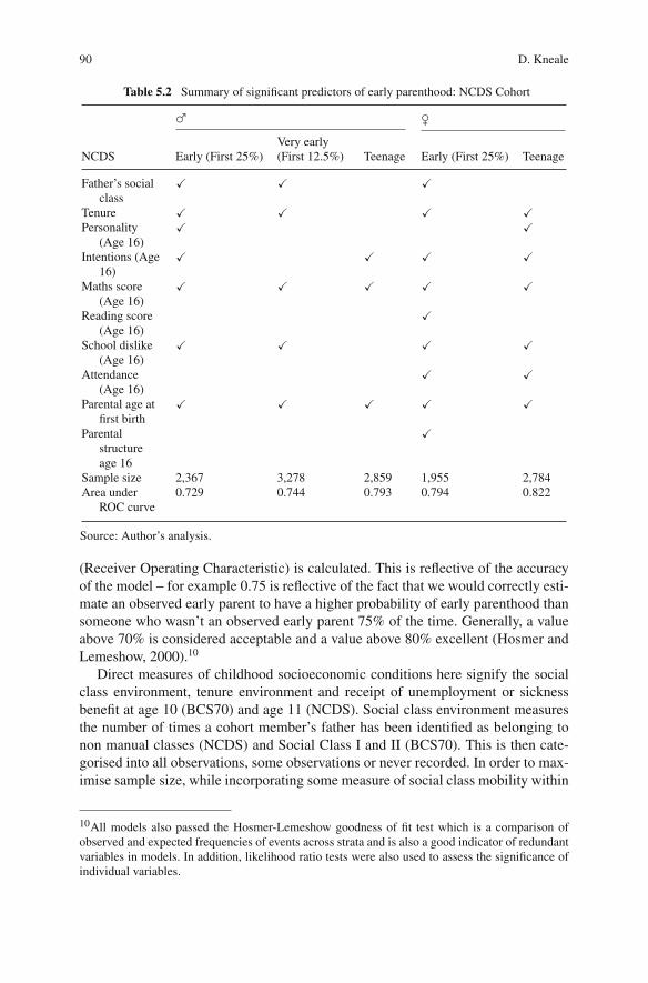
90 D. Kneale
Table 5.2 Summary of significant predictors of early parenthood: NCDS Cohort
♂ ♀Very early
NCDS Early (First 25%) (First 12.5%) Teenage Early (First 25%) Teenage
Father’s socialclass
� � �
Tenure � � � �Personality
(Age 16)� �
Intentions (Age16)
� � � �
Maths score(Age 16)
� � � � �
Reading score(Age 16)
�
School dislike(Age 16)
� � � �
Attendance(Age 16)
� �
Parental age atfirst birth
� � � � �
Parentalstructureage 16
�
Sample size 2,367 3,278 2,859 1,955 2,784Area under
ROC curve0.729 0.744 0.793 0.794 0.822
Source: Author’s analysis.
(Receiver Operating Characteristic) is calculated. This is reflective of the accuracyof the model – for example 0.75 is reflective of the fact that we would correctly esti-mate an observed early parent to have a higher probability of early parenthood thansomeone who wasn’t an observed early parent 75% of the time. Generally, a valueabove 70% is considered acceptable and a value above 80% excellent (Hosmer andLemeshow, 2000).10
Direct measures of childhood socioeconomic conditions here signify the socialclass environment, tenure environment and receipt of unemployment or sicknessbenefit at age 10 (BCS70) and age 11 (NCDS). Social class environment measuresthe number of times a cohort member’s father has been identified as belonging tonon manual classes (NCDS) and Social Class I and II (BCS70). This is then cate-gorised into all observations, some observations or never recorded. In order to max-imise sample size, while incorporating some measure of social class mobility within
10All models also passed the Hosmer-Lemeshow goodness of fit test which is a comparison ofobserved and expected frequencies of events across strata and is also a good indicator of redundantvariables in models. In addition, likelihood ratio tests were also used to assess the significance ofindividual variables.

5 Early Parenthood: Definition and Prediction in Two British Cohorts 91
Table 5.3 Summary of significant predictors of early parenthood: BCS70 Cohort
♂ ♀Early Early(First Very early (First Very early
BCS70 12.5%) (First 12.5%) Teenage 12.5%) (First 12.5%) Teenage
Father’s socialclass
� � �
Tenure � � � � �Personality
(Age 5)� �
Personality(Age 10)
�
Personality(Age 16)
� � � � �
Intentions(Age 16)
� �
Parental education � � �English
VocabularyScore (Age 5)
� �
Maths score(Age 10)
�
Reading score(Age 10)
� � �1 �1
Matrices score(Age 10)
�
School dislike(Age 16)
� � � � �1 �1
Parental age at firstbirth
� � � � � �
Parental structure(age 5)
�
Parental structure(age 16)
�
Unemployment/sicknessbenefits(Age 16)
� �
Truancy (Age 16) �Sample size 3,206 2,220 3,712 2,704 2,809 3,232Area under ROC
curve0.709 0.763 0.792 0.781 0.797 0.807
1Reading Age 10∗School Dislike Interaction TermSource: Author’s analysis.
the parental generation, this variable did not differentiate by the number of obser-vations recorded for a cohort member. For example, a cohort member in a certainsocial class at age 10 years but not observed another time would be classified ashaving all observations in that social class. This decision was taken after it was

92 D. Kneale
observed that transition between waves remained relatively stable after the birthand first waves of data collection, which in themselves have high wave responserates. In an acknowledgement that this variable is highly dependent of participationat childhood waves of data collection, a control variable was tested that measuredparticipation, although was found to be insignificant for the most part.
A similar strategy was adopted for tenure (with a breakdown given later) whilethe benefits variable was a binary variable reflecting receipt of state unemploy-ment and sickness benefits at a point in childhood. Measures of behaviour representcomponents derived from principal components analysis of Rutter Score measures(Rutter, 1967) that are common to both cohorts. These are an established set of mea-sures to monitor signs of behaviour disorders in children and teenagers includingaggression, disobedience and nervousness. These differ in their importance betweenmodels, with an index of aggression/misbehaviour particularly important for defini-tions of BCS70 fatherhood).
Teenage Fatherhood as a Choice Versus Teenage Motherhoodas an Adaptation: Breaks in the Continuum
As mentioned previously, the focus on teenage parents has seemed disproportionategiven their low, and diminishing, prevalence and a large part of the investigationhas been to examine if, in terms of predictors, their characteristics vary significantlyfrom people who became parents in their early 20s. This was not generally foundto be the case. However, a peculiarity that does stand out in terms of the resultsis the weak roles that direct measures of socioeconomic status have in the caseof teenage fatherhood. This did not apply to more extensive definitions of earlyfatherhood, and appears to break the continuum between teenage and other forms ofearly fatherhood. This phenomenon is present in both cohorts, with a total absenceof direct socioeconomic measures registering in the models of teenage fatherhood.In fact for the NCDS model of early fatherhood, few conventional predictors arefound to predict entry into this state.
All variables included in the fatherhood models presented in Tables 5.2 and 5.3have significant predictive power. Model fit statistics suggest that the models forpredicting early fatherhood provide a weaker framework of predictors than teenagefatherhood. While it would be expected that early fatherhood would constitute amore diverse group of fathers than teenage fatherhood; these results suggest thatthose joining the early fatherhood group (that already includes teenage fathers) areactually a group that is governed by a significantly different set of predictors thanthose of teenage fathers, to the point where modelling two distinct populations asa joint category produces a relatively poorer fitting model.11 This is demonstrated
11Using the Hosmer-Lemeshow test; although these results appear to be dependent on the way thatpredictions are grouped (Harrell, 2001) and are not presented here in favour of ROC curve results,that are less responsive to this.

5 Early Parenthood: Definition and Prediction in Two British Cohorts 93
Table 5.4 Goodness of fit statistics (area under ROC curve): binary definitions of earlyfatherhood
Model excluding Model excludingdirect childhood behavioural and
Definition of socioeconomic philoprogeneityCohort fatherhood measures measures∗ Full model N
NCDS Early 0.699 0.708 0.722 2,256Very early 0.702 0.719 0.728 3,205Teenage n/a 0.728 0.758 3,263
BCS70 Early 0.697 0.708 0.709 3,206Very early 0.759 0.750 0.763 2,220Teenage n/a 0.735 0.792 3,712
Source: Author’s analysis.∗Includes Dislike of School
in Table 5.4, which shows the impact of removing different sets of predictors, withhigher values representing a better prediction. Socioeconomic factors have greaterpredictive influence in more inclusive early fatherhood models but are found to beinsignificant in teenage models.
The results suggest that while transition to fatherhood in the early 20s is an adap-tation to socioeconomic factors and probably more proximal measures of socioeco-nomic status; fatherhood under 20 is associated more with behavioural, motivationaland possibly role model elements. In the case of fatherhood therefore, the contin-uum appears to move from different sets of predictive factors (from behavioural tosocioeconomic) that govern transition, while for motherhood it appears more of acontinuum moving gradually in terms of strength of prediction of the same variablegroupings.
In particular, the model for teenage fatherhood may be more of a model reflectingsexual behaviour among teenagers than conscious transition to fatherhood. Unfor-tunately, it is difficult to assess this supposition given that there are few studiesthat collect behavioural measurements with information on sexual behaviour, withthe latter not collected in the NCDS or BCS70. The inclusion of mother’s age offinishing continuous education in the BCS70 teenage fatherhood model and the sig-nificance of mother’s and father’s age at first birth in the BCS70 and NCDS modelsrespectively may represent a socioeconomic dimension or may well reflect parentalinput (including an element of having a role model), which may be moderators ofteenage sexual behaviour.12
The BCS70 teenage fatherhood model finds that having a high score for anaggressive, disobedient and destructive nature at age 16 years to be significant.In fact, those with a score in the highest quartile for this component were 4.6 times(CI: 1.9–11.2) more likely to become teenage fathers than those with a score in thelowest quartile. For BCS70, dislike of school at age 16 (discussed later) was found
12Parental environment is examined in depth in other parts of the wider research Kneale (2008).

94 D. Kneale
to be highly significant. Those who disagreed in full with a statement on dislikingschool were 83% less likely to become teenage fathers in BCS70 (odds ratio (OR):0.17; CI: 0.07–0.43). In NCDS, those who were uncertain as to the ideal age atwhich they wanted to start a family were 85% (OR: 0.15; CI: 0.03–0.44) less likelyto become teenage fathers than those who thought it ideal to start a family at age16–19 years. While some of these factors were significant in more inclusive defi-nitions of ‘early’ fatherhood; it was the fact that these were more prominent thansocioeconomic measures that defines teenage fatherhood from early fatherhood inthese models.
Teenage motherhood models show a greater continuum between teenage andother definitions of early motherhood. In addition, as might be expected, a greaterrange of covariates have been identified as significant for early motherhood thanearly fatherhood, which may indicate a less random social profile of young moth-ers. The stronger socioeconomic component suggests that early motherhood (or itsavoidance) is more of an adaptation to economic circumstance than is the case forearly fatherhood, which appears to be governed by behavioural rather than economicfactors. This could be because fathering a child as a teenager is less likely to involveco-residence with the child than is the case for teenage motherhood and is likely tohave less of a direct economic consequence. This is a temporal state however andhas been observed to change over time where some teenage fathers take up resi-dence with their children a few years after birth (Clarke et al., 2000). In essence ashas been stated, in the case of teenage fatherhood, often but not always it may be acase of modelling sexual behaviour and partnership patterns rather than consciousbehaviour.
For both cohorts, all three definitions of early motherhood are governed bysimilar sets of predictors. Universal predictors of young motherhood across bothcohorts include tenure, dislike of school at age 16, and cohort members’ mother’sage at first birth. As a generalisation, the effect of covariates wanes slightlybetween teenage and early motherhood models, with early motherhood modelsrepresenting a more diluted category, as a greater number of significant predic-tors are included in the more inclusive early motherhood models. However, insummary, it would appear that a continuum does exist between these definitionsof early motherhood, given that the predictors appear to maintain their effect(Fig. 5.2).
The Potent Effect of Disliking School on Entryinto Early Parenthood
Dislike of school itself has been examined as a predictor of early pregnancy withmixed results (Bonell et al., 2005). This is, to the author’s knowledge, the firstattempt to include ‘school dislike’ in models of entry into parenthood. Dislikeof school is found to be a potent predictor of early entry into parenthood, notonly of teenage motherhood, but also across most definitions of early parenthood

5 Early Parenthood: Definition and Prediction in Two British Cohorts 95
4
3
2
1
0
Od
ds
of
earl
y m
oth
erh
oo
d
Mix
ed o
wne
roc
cupa
tion
Onl
y co
unci
lho
usin
g
Som
e co
unci
lN
o ow
ner
occu
patio
n
Oth
er
Eac
h ad
ditio
nal
yea
r
som
ewha
tD
islik
es s
choo
l
Doe
sn’t
disl
ike
scho
olAge ofCM’s
mother atfirst birth
School dislike(baseline strongdislike of school)
Tenure (baseline owner occupation)
Teenage motherhood NCDSTeenage motherhood BCS70Early motherhood NCDSEarly motherhood BCS70
Fig. 5.2 The odds of becoming an early or teenage mother: the effects of selected covariates frommodels with full controls (Source: Author’s analysis)See Tables 5.1 and 5.2 for a full list of controls and sample sizesThe NCDS scale has been mapped into a three point scale for the purposes of Fig. 5.2 and Table5.4, but maintains a 5 point scale elsewhere in the models
(including fatherhood). Furthermore, given that dislike of school is measured ina fairly consistent way across both cohorts, its effect appears to be increasingover time.
In these data, aversion to school has been measured as the agreement or dis-agreement with the statement ‘I do not like school’. This was measured at age 16 inboth cohorts – in the NCDS as a five point scale while in the BCS70 this was as athree point scale. As the BCS70 cohort had a particularly low response of the age16 sweep (Plewis et al., 2004), a missing category was created, which was repli-cated for NCDS for comparability purposes. Among NCDS boys, 17% reported astrong dislike of school with 18% in BCS70, while the levels for girls was slightlylower at 15 and 16% respectively for NCDS and BCS70. While the level of dislike

96 D. Kneale
Table 5.5 The effect of school dislike on early parenthood: odds ratio results from parsimoniousmain effects models NCDS and BCS70
School dislike (Baseline: strong dislike of school)
Dislikes school Does not dislike Item non-Cohort Definition somewhat school response∗∗∗
NCDS Early fatherhood 0.842 0.706∗ n/aVery early fatherhood 0.816 0.522∗∗ n/aTeenage fatherhood Not significant in full model
Early motherhood 0.744 0.710∗ n/aTeenage motherhood 0.517∗∗ 0.411∗∗ n/a
BCS70 Early fatherhood 0.658∗ 0.592∗∗ 0.994Very early fatherhood 0.520∗ 0.329∗∗ 0.770Teenage fatherhood 0.209∗∗ 0.170∗∗ 0.520∗
Early motherhood 0.593∗∗ 0.507∗∗ 0.951Very early motherhood 0.557∗∗ 0.503∗∗ 0.561Teenage motherhood 0.502∗∗ 0.394∗∗ 0.656
∗∗p < 0.01; ∗p < 0.05 ∗∗∗As the item non-response for dislike of school remained fairly low forNCDS (accounting for less 20%); this category was not created.Source: Author’s analysis.
of school has remained fairly constant, the effect may be growing. The results forschool dislike in models containing a full set of significant predictors are presentedin Table 5.5.
Using those who dislike school as a baseline, it appears that even partial dis-agreement with the statement ‘I do not like school’ is highly protective againstearly parenthood, particularly for the BCS70 cohort. In the case of teenage father-hood, even partial disagreement leads to a 79% reduction in the odds of becoming ateenage father. In lognormal event history models, for entry into fatherhood betweenthe ages of 16–23 years among BCS70 males, partial disagreement with the state-ment leads to a 14% increase in the time spent childless (time ratio (TR): 1.14; CI:1.08–1.21) with full disagreement leading to an 18% increase (TR: 1.17; CI:1.09–1.25). Dislike of school produces the largest coefficients in this model, andmaintains this effect when the observation time is extended to 30 years, overshad-owing socioeconomic effects.
Dislike of school in the case of BCS70 teenage fatherhood outweighs the sig-nificance of socioeconomic measures, while it is significant alongside socioeco-nomic measures in other models. Such a finding has not been replicated in theother few studies of dislike of school (Bonell et al., 2005). In addition, in thesedata dislike of school is found to be significant alongside measures of educationalachievement, and again, overshadowing their impact in several cases. The effectswere amplified with educational attainment in BCS70, so that high achievementand liking school were mutually reinforcing protective effects against early mother-hood. From a policy perspective, this finding is highly significant and suggests thatwhere early parenthood is viewed as problematic, that school based interventions to

5 Early Parenthood: Definition and Prediction in Two British Cohorts 97
improve engagement could have measurable results. Also of interest in these dataand possibly related to dislike of school is the prominence of family building inten-tions and values as predictors of early parenthood, explored in the next subsection.
Early Parenthood as Planned Parenthood
Philoprogenitive tendencies (tendencies orientated towards children) might appearas obvious predictors of early parenthood, but they have actually received little atten-tion. This is, possibly because of the assumption that very early parenthood is theresult of unplanned pregnancy (Social Exclusion Unit, 1999), because these tenden-cies are subject to revision, because of reliance on socioeconomic theories of fer-tility or because of the lack of prospective data. In fact, family building intentionshave been more the focus as concerns of postponement and childlessness (Simp-son, 2006; Kneale and Joshi, 2008; Berrington, 2004) than early fertility, althoughsome focus has been made in studies of teenage motherhood. One example is theindex of ‘positive orientation towards early motherhood’ coined by Afable-Munsuzand colleagues, composed of a series of statements about the value of childrenwhere a latent desire for children was found among those becoming early mothers(Afable-Munsuz et al., 2005). However, a drawback of Afable-Munsuz’s study isthat it that its sample was a narrow population of African-American young womenwho were existing patrons of family planning services. East and colleagues alsofound similar results within a narrow high risk population (East et al., 2006). In thepresent data, information has been collected in a less selective way, for two cohortsof both genders.
NCDS cohort members aged 16 year olds were asked about the age at whichthey would ideally start a family, with responses grouped by age and also a categoryformed for those who intended to be childless. The modal response category for bothsexes was 22–25 years and actually only a small number of cohort members chosethe youngest category of 16–19 years13 (2% of boys and 3% of girls; those choosingunder 22 years had higher numbers; 13% of boys and 18% of girls). Almost 10%of females and 3% of males choosing the childless category became teenage par-ents. BCS70 cohort members were asked about the importance of children in theirown life to come at the age of 16 years on a three point scale. Females were mostlikely to answer that children mattered very much while males had higher levels thatanswered that children only mattered somewhat. While both measures are proxies ofintentions, both will give an indication of family building preferences as predictors,and are referred to as family building intentions from this point forward.
These data find that philoprogenitive tendencies are generally a better predictorof early motherhood than early fatherhood. Only the models for NCDS early andteenage fatherhood find these to be a mildly significant predictor. In the case of
13This is a combined category in the data of 16–17 and 18–19. There was no option to choose anyearlier.

98 D. Kneale
Table 5.6 The effect of intentions, as measured by importance of children, on early parenthood:odds ratios from parsimonious main effects models
Early motherhood Teenage motherhood
Baseline (children very important)Children somewhat important 0.540∗∗ 0.660Children not important 0.524∗∗ 0.402∗∗
Item non-response 0.672∗ 0.884
∗∗p < 0.01; ∗p < 0.05
models of early motherhood among NCDS cohort members, the age at which thecohort member regards as the ideal age at first birth operates in a non-linear fash-ion (and is modelled as a categorical variable), with those uncertain about the idealage or those selecting 26–30 years having the lowest odds of becoming early moth-ers. Among BCS70 models of early motherhood, the importance of children is asignificant predictor of teenage and early forms of motherhood with those deemingchildren to be unimportant half as likely to become early or teenage mothers thanthose deeming children to be very important. The results are presented in Table 5.6and Fig. 5.3.
These data confirm that becoming an early mother is a process based upon morethan just economic adaptation. For many young mothers, becoming an early motheris grounded in a desire to enter motherhood at an early age and a high value placedupon children. These factors remain significant even after controlling for socioe-conomic factors, educational achievement, behavioural factors and more relevantperhaps, school dislike. Early motherhood is often taken for granted solely as arational adaptation to economic factors, with poor labour market prospects leadingto some reduced opportunity costs in having an early child (Ermisch and Pevalin,2003b; Hoem, 2000). These data would demonstrate that even after accounting for
Teenage motherhood NCDS Early motherhood NCDS2
1
0
Od
ds
of
earl
y m
oth
erh
oo
d
16–1
9
20–2
1
22–2
5
26–3
0
Ove
r 30
Unc
erta
in
No
toC
hild
ren
Item
non
-re
spon
se
Fig. 5.3 The effect ofintentions, as measured byideal age at first birth, onearly parenthood: odds ratiosfrom parsimonious maineffects models(Source: Author’s analysis)Hatched lines representconfidence intervals forteenage motherhood model

5 Early Parenthood: Definition and Prediction in Two British Cohorts 99
factors influencing labour market opportunity costs (including educational factorsand dislike of school), that a social norm influencing childbearing orientationsremains for women. Should these preferences and social norms be consolidatedon a community or neighbourhood level, it would be better to think of a teenageor any early mother as being “an emerging adult participant in active multigener-ational social networks, than as a rebellious adolescent set apart from her elders”(Geronimus, 1997, p. 418).
The Dominant Role of Housing Tenure Over Social Class
A striking find in this analysis is the dominant role that housing tenure has in pre-dicting early parenthood, alongside or even eclipsing the role of social class. Resultsfrom models of fatherhood are presented in Table 5.7 while Fig. 5.2 shows someresults for motherhood. Housing tenure is one of the few predictors that moderatesentry into nearly all forms of parenthood in both cohorts (with the exception ofteenage fatherhood) in both event history and binary logistic modelling strategies.One could take the view that housing tenure represents a proxy for the type of neigh-bourhood. It could also be a direct measure of childhood socioeconomic conditions.The significance of tenure contributes to an emerging theme of the importance ofcontextual factors (Kneale, 2008).
Table 5.7 shows that tenure has an equal and sometimes greater associationwith entry into early fatherhood than it has with entry into very early fatherhood.This is mirrored to some extent in BCS70 motherhood, but is contrary to mostother results in this research that have found that common predictors among def-initions have waned with more inclusive definitions of young parenthood. Whatthis analysis, backed up by results from Event History models, adds to the storyof early transition to parenthood is that housing tenure in childhood has effects
Table 5.7 The effect of tenure on early parenthood: odds ratio results from parsimonious maineffects models NCDS and BCS70 of fatherhood
Tenure (Baseline: owner occupation)
Mixed owner Some council, noDefinition of occupation Only council owner occupation
Cohort Fatherhood tenure tenure tenure Other
NCDS Early 1.52∗∗ 1.83∗∗ 1.52 1.67∗
Very early 1.34 2.07∗∗ 2.33∗∗ 1.55Teenage Not significant in full model
BCS70 Early 1.14 1.49∗∗ 1.29 1.31Very early 1.23 1.50∗ 0.78 1.08Teenage Not significant in full model
∗∗p < 0.01; ∗p < 0.05Source: Author’s analysis.

100 D. Kneale
lasting beyond conventionally defined adolescence and well into the twenties. Inaddition, this analysis shows that in certain cases, experiencing social housing, evenif accompanied by upward movement into owner occupation, which may have beenfacilitated by the right-to-buy scheme for BCS70, has significant and lasting effects.This may well be as related to retaining community ties such as maintaining schoolor peer groups, or the lasting legacy of childhood poverty. These conclusions mir-ror those of other research that has examined childhood tenure and adult outcomes(Feinstein et al., 2008).
Conclusions: Building a Picture of Early ParenthoodPatterns in the UK
In this chapter, a definition of early parenthood bounded by the age at which onequarter of a cohort had become parents was explored. For women born in 1958,this was just over 22; for those born in 1970 it had risen to just over 24. The cor-responding figures for men were around 25 and 27. On this definition most ‘early’childbearing is no longer confined to teenagers who account for less than 13 and10% of women and 4 and 3% of men among the NCDS and BCS70 cohorts.
Early parenthood has been viewed through a wide prism in this research and asa result, this chapter illuminates several themes in the story of young parenthood inthe UK. One of the first themes identified was the inadequacy of drawing the lineat age 20. This inadequacy was revealed through univariate techniques, reinforcedby multivariate exploration of predictors. However, the story was not straightfor-ward. While teenage motherhood and early motherhood were described by similarprocesses and were essentially viewed as being on a continuum, the even smallergroup of males reporting fatherhood as teenagers appeared to be a distinct group. Inparticular, the lack of association between teenage fatherhood and socioeconomicfactors was hypothesised as reflecting teenage male sexuality and risky behaviourrather than planned fatherhood. There are greater means and incentives for womento avert the consequences of an unplanned pregnancy than males. In the case ofearly fatherhood, there was a discontinuity as the earliest (teenage) fatherhood wasassociated with behavioural factors and movement towards socioeconomic factorswith age.
Looking at particular predictors of early parenthood revealed some novel results.The dislike of school was identified as being pervasive in most models of earlyparenthood for both cohorts and genders. Having been previously linked to earlypregnancy alone, and then only in models excluding socioeconomic predictors,its continuing strength in predicting early parenthood was surprising. The path-way behind this finding is unknown. This could reflect reduced opportunity costsof entering parenthood early, as is hypothesised in literature on early parenthood(Ermisch and Pevalin, 2003b); or alternatively be more of an indicator of con-textual factors such as peer group, school or community effects; or a combina-tion of both. The significance of philoprogeneity, as measured by ideal age at firstbirth and importance of children in the NCDS and BCS70 respectively, even when

5 Early Parenthood: Definition and Prediction in Two British Cohorts 101
controlling for a battery of other predictors, may again signify the importance ofcontextual factors. Finally, the strong predictive power of housing tenure and theobserved effect of experience of poverty threw into question traditional measures ofsocial class as sole measures of socioeconomic circumstance.
Cross-cohort comparisons throughout have revealed slight nuances between thecohorts in the way these predictors operate. However, the overwhelming theme isone where the issue of comparability between cohorts can only really be made whenrelative measures are used. The inadequacy of using a teenage definition of earlyparenthood becomes particularly acute for BCS70 where the ‘absolute’ definition ofearly applies to an increasingly marginalised group. Of note as well is the increasedpotency of some predictors among the BCS70 cohort across all models suggestingthat as a whole, social polarisation in age at first birth is forming a stronger discoursein the more recent cohort.
The results presented here have composed a picture of transition to early parent-hood as being governed by numerous processes. In particular they have identifiednumerous pathways to early transition that vary from conventional predictors anddefinitions of early parenthood. These investigations have also revealed avenues forfuture work in investigating contextual predictors that are under investigation in fur-ther research (Kneale, 2008). While a number of significant predictors have beenfound to govern early parenthood, model fit statistics suggest that many more areyet to be found under the assumption that the timing of parenthood is more than justa random event.
Acknowledgments I would like to acknowledge the contribution of Heather Joshi and Jane Elliottthroughout this project both in editorial support and with analytical issues. I am very gratefulfor this support. I would also like to thank Brian Dodgeon for his help in solving data issuesencountered in this chapter. Finally, I would like to acknowledge UPTAP and the ESRC for theirfinancial support as well as all those involved with the NCDS and BCS70 studies including thecohort members themselves.
References
Afable-Munsuz, A., Speizer, I., Magnus, J. H. and Kendall, C. (2005) A positive orientation towardearly motherhood is associated with unintended pregnancy among New Orleans youth, Mater-nal and Child Health Journal, 10: 265–276.
Arai, L. (2003) Low expectations, sexual attitudes and knowledge: explaining teenage pregnancyand fertility in English communities. Insights from qualitative research, Sociological Review,51: 199–217.
Berrington, A.M. (2004) Perpetual Postponers? Women’s, men’s and couple’s fertility intentionsand subsequent fertility behaviour, Population Trends, 117: 9–19.
Berrington, A.M., Cobos Hernandez, M.I., Ingham, R. and Stevenson, J. (2005) Antecedents andoutcomes of young fatherhood: longitudinal evidence from the 1970 British Birth Cohort Study,S3RI Applications and Policy Working Papers, Southampton Statistical Sciences ResearchInstitute, Southampton University, Southampton.
Birch, D. (1992) Are You My Sister Mummy, Youth Support, London.Birch, D. (1996) The Child that Rocks the Cradle, Youth Support, London.

102 D. Kneale
Bonell, C., Allen, E., Strgange, V., Copas, A., Oakley, A., Johnson, A. and Stephenson, J. (2005)The effect of dislike of school on risk of teenage pregnancy: testing of hypotheses usinglongitudinal data from a randomised trial of sex education, Journal of Epidemiology and Com-munity Health, 59: 223–230.
Bonell, C., Fletcher, A. and McCambridge, J. (2007) Improving school ethos may reduce substancemisuse and teenage pregnancy, British medical Journal, 334: 614–616.
Bynner, R.J. and Joshi, H. (2007) Building the evidence base from longitudinal data: the aims,content and achievements of the British Birth Cohort Studies, Working Paper, Centre for Lon-gitudinal Studies, Institute of Education, University of London, London.
Bynner, J., Joshi, H. and Tsatsas, M. (2000) Obstacles and Opportunities on the Route to Adult-hood: Evidence from Rural and Urban Britain, The Smith Institute, London.
Clarke, L., Joshi, H. and Di Salvo, P. (2000) Reports and records of mothers, fathers and childrencompared, Population Trends, 102: 24–33.
East, P.L., Khoo, S.T. and Reyes, B.T. (2006) Risk and protective factors predictive of adolescentpregnancy: A longitudinal prospective study, Applied Developmental Science, 10: 188–199.
Ekert-Jaffe, O., Joshi, H., Lynch, K., Mougin, R., Rendall, M.S. and Shapiro, D. (2002) Fertility,timing of births and socio-economic status in France and Britain: social policies and occupa-tional polarization, Population (English edition), 57: 475–507.
Elliott, J. and Shepherd, P. (2006) Cohort profile: 1970 British Birth Cohort (BCS70), InternationalJournal of Epidemiology, 35: 836–843.
Ermisch, J. and Pevalin, D. (2003a) Does a ‘teen-birth’ have longer-term impacts on the mother?Evidence from the 1970 cohort study, ISER Working Papers, Institute for Social and EconomicResearch, University of Essex, Colchester.
Ermisch, J. and Pevalin, D. (2003b) Who has a child as a teenager?, ISER Working Papers, Institutefor Social and Economic Research, University of Essex, Colchester.
Feinstein, L., Lupton, R., Hammond, C., Mujtaba, T., Salter, E. and Sorhaindo, A. (2008) PublicValue of Social Housing: A Longitudinal Study of Relationships Between Housing and LifeChances, Smith Institute, London.
Ferri, E. (1993) Life at 33: The Fifth Follow-up of the National Child Development Study, NationalChildren′s Bureau, London.
Geronimus, A. (1997) Teenage childbearing and personal responsibility: an alternative view, Polit-ical Science Quarterly, 112: 405–430.
Geronimus, A. (2003) Damned if you do: culture, identity, privilege, and teenage childbearing inthe United States, Social Science & Medicine, 57: 881–893.
Goodman, A., Kaplan, G. and Walker, I. (2004) Understanding the effects of early motherhoodin Britain: the effects on mothers, IFS Working Paper 04/18, Institute for Fiscal Studies,London.
Greene, M.E. and Biddlecom, A.E. (2000) Absent and problematic men: demographic accounts ofmale reproductive histories, Population and Development Review, 26: 81–115.
Hadfield, L., Rudoe, N. and Sanderson-Mann, J. (2007) Motherhood, choice and the British media:a time to reflect, Gender and Education, 19: 255–263.
Harden, A., Brunton, G., Fletcher, A., Oakley, A., Burchett, H. and Backhans, M. (2006) Youngpeople, pregnancy and social exclusion: A systematic synthesis of research evidence to iden-tify effective, appropriate and promising approaches for prevention and support, The Evidencefor Policy and Practice Information and Co-ordinating Centre (EPPI-Centre), Social ScienceResearch Unit, Institute of Education, University of London, London.
Harrell, F.E.J. (2001) Regression Modeling Strategies; With Applications to Linear Models, Logis-tic Regression and Survival Analysis, Springer, New York.
Hobcraft, J. and Kiernan, K. (2001) Childhood poverty, early motherhood and adult exclusion,British Journal of Sociology, 52: 495–517.
Hoem, B. (2000) Entry into motherhood in Sweden: the influence of economic factors on therise and fall in fertility, 1986–1997, Demographic Research, 2, online journal available athttp://www.demographic-research.org/volumes/vol2/4/2-4.pdf

5 Early Parenthood: Definition and Prediction in Two British Cohorts 103
Hosmer, D.W.J. and Lemeshow, S. (2000) Applied Logistic Regression, Hoboken, New Jersey.Hotz V.J., McElroy-Williams, S. and Sanders, S.G. (2004) Teenage childbearing and its lifecy-
cle consequences: exploiting a natural experiment, Working Paper, Department of Economics,University of California (UCLA), Los Angeles.
Imamura, M., Tucker, J., Hannaford, P., Oliveira da Silva, M., Astin, M., Wyness, L.,Bloemenkamp, K.W.M., Jahn, A., Karro, H., Olsen, J. and Temmermen, M. (2007) Factorsassociated with teenage pregnancy in the European Union countries: a systematic review, Euro-pean Journal of Public Health, 17: 630–636.
Jaffee, S.R., Caspi, A., Moffitt, T.M., Taylor, A. and Dickson, N. (2001) Predicting early fatherhoodand whether young fathers live with their children: prospective findings and policy reconsider-ations, Journal of Child Psychology and Psychiatry, 42: 803–815.
Joshi, H. (2007) Social Polarisation in reproduction. From Boom to Bust: Fertility, Ageing andDemographic Change, CentreForum, London.
Kendall, C., Afable-Munsuz, A., Speizer, I., Avery, A., Schmidt, N. and Santelli, J. (2005) Under-standing pregnancy in a population of inner city women in New Orleans – results of qualitativeresearch, Social Science & Medicine, 60: 297–311.
Kiernan, K. and Hobcraft, J. (1997) Parental divorce during childhood: age at First intercourse,partnership and parenthood, Population Studies, 51: 41–55.
Kneale, D. (2008) Pathways to parenthood: exploring the influence of context as a predictor of earlyparenthood, Working Paper, Centre for Longitudinal Studies, Institute of Education, Universityof London, London.
Kneale, D. and Joshi, H. (2008) Postponement and childlessness – evidence from two Britishcohorts, Demographic Research, 19: 1935–1968.
Office for National Statistics (2007) Birth statistics: review of the Registrar General on birthsand patterns of family building in England and Wales, 2006, Series FM1, Office for NationalStatistics, Newport.
Plewis, I., Calderwood, L., Hawkes, D. and Nathan, G. (2004) National Child Development Studyand 1970 British Cohort Study Technical Report: Changes in the NCDS and BCS70 Popula-tions and Samples over Time, Centre for Longitudinal Studies Technical Reports, Centre forLongitudinal Studies, Institute of Education, University of London, London.
Pollock, G. (2008) Youth transitions: debates over the social context of becoming an adult, Sociol-ogy Compass, 2: 467–484.
Power, C. and Elliott, J. (2006) Cohort profile: 1958 British birth cohort (National Child Develop-ment Study), International Journal of Epidemiology, 35: 34–41.
Rendall, M.S., Clarke, L., Peters, H.E., Ranjit, N. and Verropoulou, G. (1999) Incomplete reportingof men’s fertility in the United States and Britain: a research note, Demography, 36: 135–144.
Robson, K. and Berthoud, R. (2006) Age at first birth and disadvantage among ethnic groups inBritain, Ethnic and Racial Studies, 29: 153–172.
Rutter, M. (1967) A children’s behaviour questionnaire for completion by children: preliminaryfindings, Journal of Child Psychology and Psychiatry, 8: 1–11.
Schoon, I., Bynner, J., Joshi, H., Parsons, S., Wiggins, R. and Sacker, A. (2002) The influence ofcontext, timing and duration of risk experiences for the passage from childhood to midadult-hood, Child Development, 73: 1486–1504.
Simpson, R. (2006) Childbearing on hold: a literature review, Working Paper 1, Cen-tre for Research on Families and Relationships, University of Edinburgh, Edin-burgh. www.uptap.net/reports%20and%20papers/05UPTAP%20Working%20Paper%201R.Simpson.doc
Singh, S., Darroch, J.E. and Frost, J.J. (2001) Socioeconomic disadvantage and adolescentwomen′s sexual and reproductive behaviour: the case of five developed countries, Family Plan-ning Perspectives, 33: 251–258+259.
Social Exclusion Unit (1999) Teenage Pregnancy, Social Exclusion Unit, London.Van de Kaa, D.J. (1987) Europe′s second demographic transition, Population Bulletin, 42: 1–59.

Chapter 6Currently Cohabiting: Relationship Attitudes,Expectations and Outcomes
Ernestina Coast
Introduction
The rise in cohabitation – pre-marital, non-marital and post-marital – representsone of the most significant changes in union formation patterns in many developedeconomies. The importance of cohabitation, and the public debates it generates,are reflected in the media attention it has received. In 2006, there were 2.3 mil-lion cohabiting couple families in the UK (ONS, 2007). 1 The increase in cohab-itation has occurred alongside other, related, major demographic shifts, including:rising levels of divorce; delay in entry into marriage and childbearing; and a risein the proportion of births taking place outside marriage. These are all charac-teristic of the second demographic transition (Van de Kaa, 1987; Lesthaeghe andSurkyn, 2004b), although rising levels of cohabitation in the UK have only par-tially offset declining marriage rates (Berrington and Diamond, 2000). Even withinEurope, divergent trends in the timing, duration, type and composition of cohab-iting unions have been identified (Liefbroer and Dourleijn, 2006; Kiernan, 2001;2004; Prinz, 1995). Theorising about cohabitation encompasses a broad range ofperspectives, from notions of selfish individualism and breakdown of the family(Morgan, 2000) to those of the democratic, consensual and “pure” relationship(Giddens, 1992; Beck-Gernsheim, 2002).
Cohabitation may be narrowly defined as “an intimate sexual union betweentwo unmarried partners who share the same living quarter for a sustained periodof time” (Bachrach et al., 2000), assuming a defined duration (Mynarska andBernardi, 2007). Typologies of cohabitation continue to evolve (Haskey, 2001;Martin and Thery, 2001; Casper and Bianchi, 2002), reflecting the changingnature of living arrangements in general and cohabitation in particular. As both a
E. Coast (B)Department of Social Policy, London School of Economics, Houghton Street,London, WC2A 2AE, UKe-mail: [email protected] are no annual official estimates of the cohabiting population of England and Wales, unlikelegal marital status, and trends tend to be derived from surveys such as the Labour Force Surveyand General Household Survey (GAD).
J. Stillwell et al. (eds.), Fertility, Living Arrangements, Care and Mobility, UnderstandingPopulation Trends and Processes 1, DOI 10.1007/978-1-4020-9682-2 6,C© Springer Science+Business Media B.V. 2009
105
106 E. Coast
demographic process and event, cohabitation is fuzzy (Knab, 2005), elusive (Teitlerand Reichman, 2001) and heterogeneous (Oppenheimer, 2003). Union formationin general, and cohabitation in particular, are characterised by increasing numberand complexity, with the duration of cohabiting unions appearing to be lengthening(Haskey, 2001).
Theorists seeking to explain the rise in cohabitation incorporate a wide rangeof explanatory perspectives, including: increased secularization (Lesthaeghe, 2002;Thornton et al., 1992; Lehrer, 2004); increased female labour force participation;shifts in the meaning of marriage (Allan and Crow, 2001), including a decline inits socio-cultural function (Alders and Manting, 2001); risk reduction (Mulder andManting, 1994; Galland, 1997); a decline in the cultural importance of kin; and theseparation of sex and reproduction.
Cohabitation may now be considered normative in the UK, evidenced by surveyand opinion poll data. Such attitudinal data can contribute to the body of evidenceabout prevailing social norms (and stigma) and associated behaviour. Attitudinaldata about cohabitation provide one strand of evidence about the acceptability ofcohabitation as a social institution, and contribute to the substantive demographicevidence about the role of cohabitation in contemporary societies. Responses toquestions about attitudes to cohabitation reveal the extent to which individualshave internalised norms about appropriate and ‘normal’ behaviour with respect tounion formation (Oropesa, 1996). In 1981, a special edition of the journal Alterna-tive Lifestyles dealt with cohabitation as a new form of living arrangement. Today,cohabitation has moved from being a ‘deviant’ or ‘alternative’ lifestyle choiceto one that is normative (de Vaus et al., 2005), both before and after marriage(Bumpass et al., 1991, 1995).
Context
Normative Attitudes
Attitudes are inherently subjective and virtually impossible to verify. When inter-preting attitudinal data generated by surveys, it is important to note that respondentshave to create judgements quickly in response to the question asked, often in rela-tion to some implicit standard, even if the judgements are themselves rooted in afirmly held view (Tourangeau et al., 2000). Whilst all survey questions are context-dependent, evidence shows that attitudinal questions are particularly at risk of thiseffect (Schuman and Presser, 1996). There are two broad types of attitudinal surveydata: normative and individual. Normative attitudinal responses, such as those col-lected in opinion polls, allow an individual to distance themselves from their owncircumstances. Individual attitudinal responses are, theoretically, grounded in real-ity. Norms and values relating to union formation are dynamic and respond to theinteraction between individual experiences and social responses (Bachrach et al.,2000) and both contribute to, and arise from, changes in society (Heuveline and

6 Currently Cohabiting 107
Timberlake, 2004). Attitudinal surveys are used extensively in policy debates, forexample, recent debates about the legal position of cohabiting relationship in Britainhave incorporated attitudinal information as part of their corpus of evidence for legalchange (Dey and Wasoff, 2007).
Changes in normative attitudes towards cohabitation are poorly representedbefore the final quarter of the twentieth century, mirroring the paucity of substantivedata on the prevalence of non-marital cohabitation (Gillis, 2004; Murphy, 2000a, b;Kiernan, 2004). Globally, attitudes toward pre- and non-marital cohabitation havebecome more ambivalent and less unaccepting of non-traditional living arrange-ments in general, and cohabitation in particular (Thornton, 1989). For example,Thornton’s research identifies a clear trajectory of changing attitudes towards cohab-itation in the US, with rapid changes in the 1960s and 1970s, slowing down in the1980s. Normative differences in attitudes towards cohabitation have been studiedin a variety of comparative settings, particularly in the US (Carter, 1993; Oropesa,1996; Thornton, 1989; Sweet and Bumpass, 1992; Thornton and Young-DeMarco,2001; Nock, 1998; Heuveline and Timberlake, 2004; Axinn and Thornton, 2000;Thornton, 1995), and elsewhere such as Sweden (Bernhardt, 2004; Trost, 1978),Europe (Kiernan, 2004), the UK (Haskey, 2001; Barlow et al., 2001), and Poland(Kwak, 1996; Mynarska and Bernardi, 2007). An increase in the acceptability ofcohabitation can reasonably be interpreted as evidence for weakening of the socialnorms surrounding marriage, referred to variously as the deinstitutionalisation ofmarriage (Cherlin, 2004), demariage (Thery, 1993) and the disestablishment of mar-riage (Coontz, 2004, quoting Cott).
Responses to normative questions are grounded in a specific time and context.Because cohabitation (and other forms of intimate relationship) are dynamic – amoving target, responses to questions about the acceptability of cohabitation posedin the 1980s potentially have different meanings than responses to questions posedin the twenty-first century, even if the question wording and response categoriesare exactly the same. In Britain, two key sources of population-level attitudi-nal data about cohabitation are the British Household Panel Survey (BHPS) andBritish Social Attitudes Survey (BSA). The data reported here update and expandupon Haskey’s (2001) review of population-level attitudes towards cohabitation inBritain.
The BHPS has asked a series of repeated self-completion questions about atti-tudes towards cohabitation using Likert-scale responses. It is important to note thatthe phrasing of the self-completion questions changed at Wave 8 (1998). Previouswaves (1992, 1994, 1996) used the statement “Living together outside of marriageis always wrong”. Subsequent waves (1998–2004) used the statement “It is alrightfor people to live together even if they have no interest in considering marriage”.The BHPS also includes a separate youth questionnaire for all household membersaged 11–15 years (inclusive), incorporating the repeated statement response “Liv-ing together outside of marriage is always wrong”. Interestingly, whilst this phras-ing was changed for adult BHPS respondents, it has remained constant for youthrespondents.

108 E. Coast
The annual cross-sectional BSA survey has included a combination of repeatand ad hoc2 questions about attitudes to cohabitation (Haskey, 2001; Barlow, 2004).This review focuses on repeat elements, namely attitude responses to statements in1989, 1994, 2000 and 2002 (Do you agree or disagree? It is a good idea for a couplewho intend to get married to live together first” “Do you agree or disagree? It is allright for a couple to live together without intending to get married.” “Do you agreeor disagree? People who want children ought to get married”). Table 6.1 summarisesnormative data relating to cohabitation in the BHPS (1992–2004). More than twothirds of respondents have reported agreement with the statement “It is alright forpeople to live together even if they have no interest in considering marriage” in eachof four successive waves.
Disaggregating responses to statements about cohabitation by birth cohort, aclear generational pattern emerges, with older cohorts much less likely to approveof non-marital cohabitation relative to younger cohorts. This is mirrored by trendsin reported ever-cohabitation by birth cohort. Less than 3% of respondents born
Table 6.1 Percentage distribution of respondents’ attitudes to cohabitation in general, 1992–2004
“Living together outside ofmarriage is always wrong”
“It is alright for people to live togethereven if they have no interest inconsidering marriage”
1992 1994 1996 1998 2000 2002 2004
Strongly agree/Agree 16.7 14.7 14.1 66.4 69.7 68.4 69.4Neither agree nor disagree 30 28.9 28.5 21.4 19.5 20.3 20Strong disagree/ Disagree 53.3 56.4 57.4 12.2 10.8 11.3 10.6N 9,284 8,940 9,027 10,427 14,799 15,215 14,341
Note the phrasing of the self-completion questions changed at Wave 8 (1998). Previous waves(2, 4, 6) used the statement “Living together outside of marriage is always wrong”. Subsequentwaves (8, 10, 12, 14) used the statement “It is alright for people to live together even if they haveno interest in considering marriage”. n = valid cases, excluding missing or don’t know responses.Source: BHPS 1992–2004 documentation and questionnaires: http://www.iser.essex.ac.uk/ulsc/bhps/doc/volb/indexes/subjcat20.php#Values,%20Opinions%20and%20AttitudesAccessed30/06/08.
2BSA ad hoc questions on attitudes towards cohabitation are as follows: 1986 “Do you agree ordisagree? As a society we ought to do more to safeguard the institution of marriage”. 1986 “Doyou agree or disagree? Most people nowadays take marriage too lightly”. 1989 “Do you agree ordisagree? Personal freedom is more important than the companionship of marriage”. 1989 “If youwere advising a young (wo)man, which of the following ways would you recommend? Live alonewith no partner /Live with a partner and not marry / Live with a partner and then marry/ Marryfirst”. 1989 and 1994 “Do you agree or disagree? The main advantage of marriage is that is givesfinancial security”. 1994 “Imagine an unmarried couple who decide to have a child, but do notmarry? What would your general opinion be?”. 2000 “Many people who live together withoutgetting married are just scared of commitment”. 2000 “There is no point getting married - it’sonly a piece of paper”.

6 Currently Cohabiting 109
Agree statement male Ever cohabited male Ever cohabited femaleAgree statement female
1930 1940 1950 1960 19701920
100
90
80
70
60
50
40
30
20
10
0Per
cen
tag
e (s
tro
ng
ly)
agre
e re
spo
nse
to
the
stat
emen
t Ò
it is
alr
igh
t fo
r p
eop
le t
oliv
e to
get
her
eve
n if
th
ey h
ave
no
inte
rest
in c
on
sid
erin
g m
arri
age
Birth cohort
70
60
50
40
30
20
10
0
Percen
tage ever co
hab
ited
Fig. 6.1 Distribution of attitudes towards, and experience of, cohabitation, by birth cohort andsex, 1920–1970(Source: BHPS, 2004.)
in the 1920s reported ever having cohabited, compared with 57% of respondentsborn in the 1970s. Men appear to have slightly more accepting attitudes towardscohabitation, although this differential is negligible for more recent birth cohorts(Fig. 6.1).
Individuals who have ever-cohabited are significantly (p<0.000) more likely toreport approving attitudes towards cohabitation, with just 1.7% of ever-cohabitingrespondents disagreeing with the statement “It is alright for people to live togethereven if they have no interest in considering marriage”. This significant relation-ship holds for all birth cohorts. It is possible to examine whether an individ-ual’s attitude towards cohabitation in general changes over the six year inter-val between the first (1998) and most recent (2004) waves including attitudinalstatements on non-marital cohabitation. Normative attitudes reported in the BHPSare relatively stable. Nearly three quarters (74%) of respondents report the samebroad response in both 1998 and 2004. Of those that change their broad responsecategory over the period, the majority shift towards a more accepting attitudeover time.
Successive generations tend to have less traditional attitudes when comparedwith preceding generations, a function of both generation succession and intra-generational change (Scott et al., 1996). Adolescents’ attitudes provide insight intothe probable trajectory of normative attitudes and behaviours in the near future.The attitudes of adolescents are important for determining future choices (Burt andScott, 2002; Manning et al., 2007 ), with young adults who approve of cohabita-tion more likely to enter into a cohabiting relationship (Axinn and Thornton, 1993).Successive BHPS waves (1994, 1999, 2000, 2001, 2005) asked young people aged

110 E. Coast
Table 6.2 Percentage distribution of youths aged 11–15 years (inclusive) response to the questionstatement “Living together outside of marriage is always wrong”
Living together outside of marriage is always wrong
1994 1999 2000 2001 2005
Strongly agree/Agree 19.0 12.8 11.9 10.6 13.3Neither agree nor disagree 21.2 27.9 26.7 23.5 30.8Strong disagree/Disagree 59.8 59.3 61.4 65.9 55.9n 759 929 1,409 1,404 1,401
n = valid cases, excluding missing or don’t know responses.Source: BHPS 1994–2005 documentation and questionnaires: http://www.iser.essex.ac.uk/ulsc/bhps/doc/volb/indexes/subjcat20.php#Values,%20Opinions%20and%20Attitudes.
11–15 years their attitude toward the statement “Living together outside of mar-riage is always wrong”. Treating the data as cross-sectional for descriptive pur-poses, the broad pattern appears to be one of increasing ambivalence, with nearlyone third of respondents neither agreeing nor disagreeing with the statement in 2005(Table 6.2).
When using panel data to examine normative attitudes, it is useful to try todisentangle whether observed changes in attitudes develop because the observedindividuals have adopted new attitudes or because new individuals with differ-ent attitudes have entered the population. For example, the five year gap betweenthe 1994 and 1999 rounds of the youth questions on cohabitation meant thatvery few of those interviewed in 1994 would have still been eligible for inter-view in 1999. By contrast, repeat of the questions in successive years (1999,2000, 2001) would have repeatedly captured a proportion of the population whoremained within the 11–15 age group. The BSA has asked a set of questionsabout attitudes towards cohabitation in subsequent survey years (1994, 1998,2000, 2002). The proportion of individuals expressing negative views aboutcohabitation, and its relation to marriage, has declined across all age groups(Fig. 6.2).
Questions about attitudes towards cohabitation are just one element of the bat-tery of attitudinal questions contained in surveys such as the BSA. For example, theBSA has asked questions annually about non-marital (pre- and extra-) sexual rela-tionships since 1983. It is important to note that attitudes of increased acceptance ofcohabitation have changed more rapidly than attitudes towards other aspects of inti-mate relationships such as extra-marital sex and same-sex relationships. As such,cohabitation has emerged as an aspect of intimate relationships that has come tobe regarded differently (perhaps separately?) from other indicators of sexual free-dom (Murphy, 2000b; Reynolds and Mansfield, 1999). Acceptance of cohabitationis likely to increase in the future, a function of the social processes of cohort replace-ment, socialisation and social diffusion (Seltzer, 2004).

6 Currently Cohabiting 111
50
45
40
35
30
25
20
15
10
5
0
Per
cen
tag
e o
f re
spo
nd
ents
1994
2002
1994
2002
1994
2002
18–34 35–54 55+
1994
2002
1994
2002
1994
2002
18–34 35–54 55+
1994
2002
1994
2002
1994
2002
18–34 35–54 55+It is all right for a
couple to live togetherwithout intending to
get married
It is a good ideafor a couple who intendto get married to live
together first
People who wantchildren ought to get
married
Fig. 6.2 Percentage distribution, by age group,3 of respondents who disagree, or strongly disagree,with statements about cohabitation and marriage, 1994 and 2002(Source: BSA.)
Individual Attitudes, Expectations and Outcomes
In the USA, a limited number of studies have examined the effects of cohabitors’own assessments of their relationship on union outcomes. Brown (2000) combinesboth relationship assessments (positive versus negative) and expectations. Researchelsewhere has considered the relationship between relationship expectations andoutcomes. For example, Manning and Smock (1995) found that cohabiting couplesthat express an intention to marry are four times more likely to marry comparedwith couples with no reported plans to marry. Reports of plans or expectations tomarry by cohabiters can be interpreted as indicative of cohabiting unions repre-senting a transitional state leading to marriage. Relationship expectations cannot beused as proxy indicators of relationship ‘quality’. For example, an expectation ofrelationship transition to marriage might be an expression of a perceived absence ofalternatives to the current cohabiting relationship. Similarly, an expectation of split-ting up may be an expectation based on externalities such as forthcoming universityattendance in another part of the country.
Much research compares cohabitation to marriage, and compared to marriedcouples, cohabiting couples differ in several distinct ways (Bachrach et al., 2000)including higher rates of union instability (Waite and Gallagher, 2000; Ermisch andFrancesconi, 2000; Bouchard, 2006). It is important to note, however, that muchof the earlier research into the dissolution of cohabiting versus married partner-ships used data on unions from the 1970s and early 1980s when cohabitation was
3Age at time of interview.

112 E. Coast
much rarer (de Vaus et al., 2005). The influence of cohabitation has been examinedon a wide range of outcomes, and is associated with: relationship dissatisfaction(DeMaris, 1984); higher levels of conflict and violence (Thomson and Collela, 1992;Forste, 2002; Kenney and McLanahan, 2006); lower quality of partner communica-tion (Cohan and Kleinbaum, 2002); lower levels of sexual exclusivity (Forste andTanfer, 1996), greater dependency on family of origin (Rindfuss and VandenHeuvel,1990); and lower relationship quality (Brown and Booth, 1996).
Relationship expectation reports are cross-sectional, and it might be that an indi-vidual entered into a cohabiting relationship with no expectations of marriage, butthat these expectations changed over time. The absence of expectations to marrycan represent one of three positions: firstly, an ideological position that opposesmarriage; secondly, an assessment that their current partner is not marriage mate-rial, but an absence of an ideological opposition to marriage per se; thirdly, theyhave yet to transition to thinking about marriage. The purpose of looking at rela-tionship expectations is to throw some light on whether cohabitation represents analternative to marriage, or an integral component of the transition to marriage. Forexample, older cohabitors tend to be more likely to report their relationship as analternative to marriage, whereas younger cohabitors are more likely to report cohab-itation as a precursor to marriage (King and Scott, 2005). It is important to anal-yse gendered relationship expectations and attitudes. Considerable research into thegendered aspects of marriage has revealed ‘his’ and ‘her’ marriages, first identifiedby Bernard and Bernard (1982) and subsequently Fowers (1991), and it is reason-able to hypothesise that there are ‘his’ and ‘her’ cohabitations.
Analyses
Data
This research uses data from the BHPS to analyse individuals’ relationship expecta-tions and subsequent reported relationship behaviour (University of Essex, 2006). Itdeals with the relationship intentions of those individuals who report a non-maritalcohabiting partner. How do cohabiting relationship expectations differ by age, sex,previous relationship history and parenthood? For people in cohabiting relation-ships, how do attitudes towards cohabitation differ by age, sex, previous relation-ship history and parenthood? Do individuals achieve their relationship expectations?How are cohabiting couples’ relationship expectations associated with relationshipoutcomes (marriage, separation, continued cohabitation)?
Begun in 1991, the BHPS surveys approximately 5,000 households annually. Inthe eighth wave, in 1998, and again in the thirteenth wave, in 2003, individualsaged 16 and above who were in cohabiting relationships were asked about theirexpectations of this cohabiting relationship. They were shown a card with a rangeof responses and asked to “read out the number of the statement which you feelapplies most closely to your current relationship”. The responses included: “Plan-ning to marry”, “Probably get married”, “Just live together”, “No thought to the

6 Currently Cohabiting 113
future”, “Don’t know” and “Other”. A supplementary question was asked of thoserespondents who replied “Don’t know” or “Just live together”. The supplementaryquestion also used a showcard, and asked for a response to the statement “howlikely it is that you will ever get married (or remarried) to anyone in the future?”.The responses included: “Very likely”, “Likely”, “Unlikely”, “Very unlikely” and“Don’t know”.
Cohabiting respondents were asked a series of questions about their perceptionsabout cohabitation in general. It is important to note that this series of questions didnot explicitly ask respondents to reflect upon their own current cohabiting relation-ship, but the questions did explicitly compare cohabiting relationships to marriage,rather than to any other form of union. The questions were: “Do you think there areany advantages in living as a couple, rather than being married?” and “Do you thinkthere are any disadvantages in living as a couple, rather than being married?”. If arespondent answered yes to either of these questions, they were prompted for openended responses (up to two mentions) with the question “What do you think are the(dis)advantages of living as a couple?”
Also in the eighth wave, in 1998, and again in the thirteenth wave, in 2003, indi-viduals aged 16 and above were asked “Do you have a steady relationship with amale or female friend whom you think of as your ‘partner’, even though you arenot living together?” Respondents that reported such a partner were then asked theirintentions about this relationship, based on show card responses to the question“Please look at this card and read out the number of the statement you feel appliesmost closely to this relationship?”, with responses of “Expect to marry”, “Expect tocohabit”, “No plans to marry or cohabit” and “Don’t know”. For those individualswho reported a partner, but did not report an expectation of marriage or cohab-itation with this partner, a supplementary showcard response question was asked“Can you please look at this card and tell me how likely it is that you will everget married or remarried to anyone in the future?”, with responses of “Very likely”,“Likely” “Unlikely”, “Very unlikely” and “Don’t know”. Because the BHPS onlycollects data from coresidential members of a household, data and analyses on non-co-residential partners are restricted to those individuals who are members of theBHPS sample, and not their partners.
Descriptive Overview
Cohabitation is heterogeneous, involving pre-, intra- and post-marital cohabitingrelationships (Table 6.3). For women and men born in the 1970s, 72 and 75%,respectively, of first unions were cohabiting. The normative status of cohabitationas a first type of union is underlined by examining the relatively small numbers ofindividuals born in the 1980s and aged 16 and over included in the BHPS. Of thosemembers of this most recent cohort who have entered live-in unions (n = 470), 91%report cohabitation as the first type of union, underlining the primacy of cohabitationas first union (Berthoud, 2000).

114 E. Coast
Table 6.3 Percentage distribution of respondents reporting a cohabiting relationship, by sex, 1998and 2003
1998 2003n = 1,187 n = 1,511
Male Female Male Female
Current legal marital status– Married 1.2 1.9 1.1 0.5– Separated 3.2 3.2 3.7 1.9– Divorced 24.0 25.6 22.9 25.8– Widowed 1.4 2.3 1.2 2.3– Never married 70.1 67.0 71.0 69.5
Parent 32.0 40.8 40.5 50.8Length of cohabiting
relationship at interview– < 6 months 15.6 16.4 6.9 8.8– 6–12 months 13.1 13.8 10.7 9.5– 1–2 years 18.2 16.4 17.2 17.9– 2–5 years 31.3 29.4 29.8 30.4– > 5 years 21.8 23.9 35.4 33.6
Source: BHPS, 1998 and 2003, author’s analysis.
In terms of the characteristics of individual cohabiting couples, more than half(55.1%) of all cohabiting relationships in 2003 where neither partner had been pre-viously married, involved both partners born in the 1970s.
Cohabiting Relationship: Attitudes
Cohabiting relationship attitudes and expectations were collected in both 1998 and2003. When examining whether relationship expectations are achieved, data areused from the 1998 wave forwards to the most recent interview for each individ-ual. The short time span between the 2003 wave of relationship expectation dataand the most recent published wave of the BHPS (2005) precludes detailed analysisof relationship outcomes from the 2003 wave forwards.
An individual can report both advantages and disadvantages of cohabitationwhen compared to marriage, and the two are not mutually exclusive. In 1998 and2003 the majority of cohabiting respondents reported neither an advantage nor a dis-advantage (47 and 55% respectively) (Table 6.4). In 2003 less than one third of indi-viduals in cohabiting relationships reported that there was an advantage to living in acohabiting relationship when compared to marriage. Responses from never-marriedindividuals are based on perceptions about marriage, rather than direct experience ofit. Overall, there is no significant relationship between sex and whether an individ-ual reports an advantage to cohabitation compared to marriage. However, respon-dents who are parents are significantly (1998 p<0.005; 2003 p<0.000) less likelyto report advantages of cohabitation compared to non-parents. Examining in detail

6 Currently Cohabiting 115
Table 6.4 Percentage distribution of attitudes about cohabitation, currently cohabiting respon-dents, 1998 and 2003
1998 2003n=1,115 n=1,514
Advantages in living as a couple 40.0 32.0First mentioned advantage1
– trial marriage 30.7 23.6– no legal ties 29.8 24.5– improves relationship 5.2 3.6– previous bad marriage 1.6 2.7– personal independence 10.0 10.9– financial advantage 16.1 22.2– companionship 2.0 3.1– prefer cohabitation 1.4 1.3– other 3.2 8.2
Disadvantages in living as couple 26.7 23.6First mentioned disadvantage2
– financial insecurity 39.0 30.4– no legal status 16.6 32.1– effects on children 5.4 6.2– lack of commitment 15.6 9.6– social stigma 16.3 11.3– other 7.1 10.4
1 Second mentioned advantages were collected in both 1998 and 2003,but have not been included in analyses here due to the relatively smallnumbers (n = 44, n = 33, respectively) reporting a second advantage.2 Second mentioned disadvantages were collected in both 1998 and2003, but have not been included in analyses here due to the relativelysmall numbers (n = 16, n = 44, respectively) reporting a second disad-vantage. Source: BHPS, 1998 and 2003, author’s analysis.
the four most commonly reported advantages of cohabitation (trial marriage, nolegal ties, personal independence and financial advantage), there are no significantdifferences by sex. Parenthood status is significantly related (1998 p<0.001; 2003p<0.005), with non-parents more likely to report trial marriage, and parents morelikely to report personal independence and the absence of legal ties as advantagesof cohabitation.
Approximately one quarter of respondents report disadvantages in living as acouple in both 1998 and 2003, with women significantly more likely to report dis-advantages compared to men if they had a previous live-in relationship (p<0.000)or were a parent (p<0.050). For the subset of individuals whose cohabiting rela-tionships extended across the 1998 and 2003 interviews (n = 144), it is possible toexamine the consistency of responses over time. Of those individuals reporting atti-tudes on the same cohabiting union in 1998 and 2003 (n = 132), overall attitudes arefairly consistent, reporting the same response to whether there are advantages or dis-advantages (62.1 and 68.9%) to cohabitation. This suggests that those individuals inlong duration cohabiting relationships have well-established attitudes towards their

116 E. Coast
Table 6.5 Percentage distribution of responses to the statement “How likely is it that you will everget married to anyone in the future?”, by currently cohabiting, never married respondents with noplans to marry their current partner, by sex, 1998 and 2003
1998 2003n = 268 n = 401
Male Female Male Female
Don’t know 11.6 8.6 10.2 6.8Very likely 4.7 5.8 3.1 3.4Likely 24.0 28.8 18.9 23.9Unlikely 25.6 38.8 40.8 42.9Very unlikely 34.1 18.0 27.0 22.9
Source: BHPS, 1998 and 2003, author’s analysis.
union. Substantial proportions of never-married, currently cohabiting respondentswith no expectation of marriage for the current cohabiting relationship, report thatthey are unlikely or very unlikely ever to marry, with 67.8 and 65.8% of men andwomen, respectively, reporting this expectation (Table 6.5).
The percentage of those respondents who reported no plans to marry in 1998, andthought it was (very) unlikely they would ever marry, did actually go on to marry(18.5% split up and 71.4% were still cohabiting at their most recent interview).
Cohabiting Relationships: Expectations
If cohabitation is part of the marriage process, then one might reasonably expectindividuals to respond that they have plans to marry the longer they have cohab-ited. For cohabiting individuals interviewed in 2003, the relationship between theduration of the cohabiting relationship is significantly (p<0.000) associated withrelationship intentions (Table 6.6).
The majority of individuals in what might be described as long-term cohabitingrelationships do not report an expectation of marriage, but of continued cohabi-
Table 6.6 Percentage distribution of future relationship expectations, by duration of current cohab-iting relationship, 2003
Future of current cohabiting relationship
Plan to marry Probably marry Live together
Duration of currentcohabiting relationship
< 1 year 30.5 38.0 31.61–2 years 29.9 44.4 25.72–5 years 19.8 48.5 31.7> 5 years 9.2 33.4 57.4
n = 1,1015 respondentsSource: BHPS, 2003, author’s analysis.

6 Currently Cohabiting 117
Table 6.7 Distribution of expectations by prior relationship history, 1993 and 2003
Future of currentcohabitingrelationship
1998 2003(n = 1,007) (n = 1,343)
No previous live-inrelationship
Prior live-inrelationship
No previous live-inrelationship
Prior live-inrelationship
Planning to marry 24.7 13.3 22.7 16.9Probably marry 46.8 37.6 47.2 33.7Live together 28.5 49.0 30.1 49.4
Source: BHPS, 1998 and 2003, author’s analysis.
tation. The BHPS does not collect information on whether a couple has becomeengaged – in and of itself not a formal or binding event – but it is reasonable to inferthat individuals with relatively short-lived cohabiting relationships have moved inbecause a marriage is already planned. Individuals who had a prior live-in relation-ship (whether married or cohabiting) are significantly (p < 0.000 for both 1998and 2003) more likely to report an intention to continue cohabiting compared withindividuals who have not had a prior live-in relationship (Table 6.7).
Cohabiting Relationships: Outcomes and Expectations
Table 6.8 shows the distribution of outcomes of cohabiting relationships identified in1998. For never-married, childless respondents interviewed in 1998, the subsequentbirth of a child within the relationship is significantly (p<0.050) associated with therelationship outcome, with subsequent parents more likely to continue to cohabitand less likely to marry compared to non-parents.
What proportion of individuals achieve their relationship expectations? Basedon responses to questions about cohabiting relationships in 1998, it is possible toexamine the outcome of those relationships to the most recent interview (Table 6.9).
For those respondents that reported a ‘definite’ expectation (plan to marry/ prob-ably marry/continue to cohabit), there is a highly significant (p<0.000) relationshipbetween expectation and outcome, for both men and women and for both parents
Table 6.8 Percentage distribution of relationship outcomes, for cohabiting unions identified in1998.
Subsequent outcome
Split up Marry Continue to cohabit
All 16.6 30.3 53.1Never married 17.3 31.2 51.5Ever-married 15.1 28.4 56.5
Source: BHPS, 1998 and 2003, author’s analysis.

118 E. Coast
Table 6.9 Percentage distribution of outcome of cohabiting relationships by relationship expecta-tions expressed in 1998
Future of current relationship
Outcome todate
Plan tomarry
Probablymarry
Livetogether
No thoughtto future
Do notknow
Split up 0.9 7.0 6.6 1.3 0.1Marry 10.7 13.6 4.8 0.6 0.1Continue to
cohabit4.2 20.9 23.9 3.7 1.5
Source: BHPS, 1998 and 2003, author’s analysis.
and non-parents at the time of interview. More than two thirds (67.9%) of thoseindividuals who reported that they planned to marry their cohabiting partner thenwent on to marry that partner.
In order to examine concordance and discordance of relationship expectationsbetween men and women, we select couples where both partners provided fullresponses to questions about the advantages and disadvantages of cohabitation, andtheir expectations of the current cohabiting relationship (Table 6.10). Analyses hereare restricted to those individuals reporting on cohabiting unions which representedtheir first ever live-in relationship. Because analyses are based on fully respond-ing couples, the responses may be biased for homogeneity of response (Berrington,2004). It is possible to identify whether anyone else was present during the BHPSinterview, but interviewers report very low levels of influence of third parties whenthey are present during interview. 4
Levels of concordance (either both report “Yes” or both report “No”) within cou-ples are high, with most concordance for “No” responses to questions about dis-advantages and advantages of cohabitation when compared with marriage. Whereboth partners report an advantage of cohabitation over marriage, the most commonconcordant response is as a trial marriage, in both 1998 and 2003 (32.4 and 26.5%
Table 6.10 Percentage distribution of couple concordance on attitudes towards cohabitation
1998 2003n=168 couples n=231 couples
Couple concordant % Couple concordant %
Advantages 65.4 64.9Disadvantages 63.9 74.0
Source: BHPS, 1998 and 2003, author’s analysis.
4For example, in 1998, of 187 interviews of currently cohabiting couples, 108 (58 per cent) recorda third party as being present. 96 of these 108 interviews (89 per cent) are coded as no influenceexerted by the third party.

6 Currently Cohabiting 119
of couples). Levels of agreement within couples about specific disadvantages ofcohabitation are much lower, although financial insecurity is the most commonlymentioned where both partners report a disadvantage.
In terms of future expectations about their current cohabiting union, there arehigh levels of concordance within couples. Of course, concordance does not equalachievement of these desires, concordant couples may still be disappointed in thefuture.
For those cohabiting couples interviewed in 1998, it is possible to examine theirrelationship outcomes by the date of their last interview (Table 6.11). 81.5% of thosecouples who agreed in 1998 that they planned to marry did go on to marry, whereasonly 39.5% of those couples who agreed they would probably get married went onto convert their relationship to a marriage. Three fifths of couples who agreed in1998 that they would continue to cohabit were still cohabiting at their most recentinterview wave in the BHPS.
Table 6.11 Couple relationship expectations, currently cohabiting couples, 1998 and 2003
1998 2003n = 137 couples n = 196 couples
Women Women
Planning to Probably get Just live Planning to Probably get Just liveMen marry married together marry married together
Planning tomarry
20.4 8.0 0.7 19.9 5.1 1.0
Probably getmarried
3.6 43.8 5.8 3.6 37.8 10.7
Just livetogether
0 5.8 11.7 0 4.6 17.3
Source: BHPS, 1998 and 2003, author’s analysis.
Discussion
The data reported here underline the heterogeneity of cohabitation, a heterogeneitythat raises challenges for researchers to make generalisations about the processesthat underlie it, the forms it takes, and the intentions that people report.
In this study the majority of cohabitors assert that they will marry their partner(including both “Plan to marry” and “Probably marry”), in keeping with US analy-ses (Bumpass and Sweet, 1989; Carlson et al., 2004; Manning and Smock, 2002).Such responses would imply that cohabitation is one element of the process of mar-riage, and that cohabitation represents a considered step on the pathway to marriage.However, what we cannot tell is whether these intentions to marry preceded becom-ing a co-residential couple, or whether they emerged as a result of having co-resided.Recent work suggests that many (if not most) cohabiting couples ‘slide’ rather than

120 E. Coast
‘decide’ into a co-residential cohabiting relationship (Stanley et al., 2006), echoingfindings from Lindsay’s (2000) work in Australia.
Current cohabitees who have a previous live-in relationship and are already par-ents are more likely to report an expectation of cohabitation rather than marriage,echoing work in the US (Bumpass et al., 1991). Smart and Stevens’ (2000) study ofcohabiting families in Britain reports that some cohabiting mothers prefer to con-tinue cohabiting rather than marry a man whom they were uncertain they could relyon for support or to enter into single parenthood. The reported advantages and disad-vantages of cohabitation relative to marriage among current cohabitees in the BHPSsuggest that, at least for never-married respondents, assessing compatibility througha ‘trial marriage’ is important. King and Scott’s (2005) work in the US using theNational Survey of Families and Households, reports that compatibility assessmentby younger cohabitors was a key reason for cohabitation.
The wording of survey questions such as those included in the BHPS tend to posestatements about cohabitation relative to marriage. This standpoint reflects muchof the broader academic endeavour surrounding cohabitation, which has debatedwhether cohabitation is a prelude to marriage, or whether it is an alternative tomarriage. A body of work has suggested, however, that a more productive line ofenquiry might be to view cohabitation as an alternative to being single (Rindfussand VandenHeuvel, 1990) and/or a progression of an intimate non-co-residentialrelationship (Casper and Bianchi, 2002; McGinnis, 2003). It is also quite possiblethat each rationale may operate at different points over time for an individual.
Datasets, including the BHPS, rarely collect information on engagements, whichaffect the entering into, and dissolution of, cohabiting unions. If couples are cohab-iting as a result of engagement with an intention to marry, then engagement-drivencohabitation explains in part both the rise in cohabitation and delays in marriage.Such compositional shifts (Oppenheimer, 2003) in cohabitation, further complicateits study. One possible reason, rarely explored, for reported intentions not to converta cohabiting union into a marital union, is that of the costs of a wedding (Kravdal,1999). Whilst a marriage in England and Wales costs approximately £100, the costof a wedding can run to tens of thousands of pounds, and for many people, themarriage and the wedding are indivisible as processes (Otnes and Pleck, 2003).Such cost-related concerns can become more sharply focused if one or both of thecohabiting partners is a parent, notwithstanding other economic needs identified asprerequisite to marriage (Gibson-Davis et al., 2005).
Future research needs to widen the pool of potential couples available to enterinto a co-residential union, whether cohabiting or married, and their relationshipintentions. ‘Living-apart-together’ (LAT) relationships, in which two partnersregard themselves as a couple but do not cohabit, have recently been recog-nised in the social science literature (Levin and Trost, 1999; Bawin-Legros andGauthier, 2001; Karlsson and Borell, 2002; Borell and Karlsson, 2003; Milanand Peters, 2003; Levin, 2004; de Jong Gierveld, 2004; Haskey, 2005; Lewisand Haskey, 2006) as an emergent form of living arrangement. It is estimatedthat there are some two million men and women in Great Britain who reporthaving a partner who lives in another household (Haskey, 2005). The BHPS

6 Currently Cohabiting 121
has collected information from sample members on non-co-residential partners,but does not collect detailed information from or about these non-co-residentialpartners. As people’s living arrangements and households become smaller andmore complex, their commitments and networks outside of the traditional ‘house-hold’ tend to become greater, meaning that social science research needs to betterunderstand and reflect non-household-based definitions and sources of information(ESRC, 2006).
There is a need for more finely grained qualitative research into the processesunderlying cohabiting unions, including their formation and dissolution. The vastmajority of research on cohabitation is based in the U.S. and is quantitative (Lewis,2001). Large-scale, representative, quantitative datasets such as the BHPS give ussome clues as to potential avenues for further investigation. However, they cannotfully account for the rapidly changing role of cohabitation in contemporary society.There is an emergent body of qualitative research into cohabitation, including itsprocesses and meaning (Manning and Smock, 2005; Sassler, 2004; Lindsay, 2000).There is a need to understand better what trends in cohabitation in particular, andliving arrangements in general, actually signify (Oppenheimer, 2003). Cohabitationhas emerged relatively recently and rapidly as a normative behaviour in many set-tings, and is therefore in a situation of flux and change (Seltzer, 2000). The reasonsunderlying decisions (whether articulated explicitly or otherwise) to cohabit may,therefore, also be subject to rapid change, making cohabitation very much a movingtarget to study.
Acknowledgment This research was based on the British Households Panel Survey ConsolidatedMarital, Cohabitation and Fertility Histories, 1991–2006, produced by the Institute for Social andEconomic Research at the University of Essex. Access to the data was via the Economic and SocialData Service, SN: 5629.
References
Alders, M.P.C. and Manting, D. (2001) Household scenarios for the European Union, 1995–202,Genus, LVII (2): 17–48.
Allan, G. and Crow, G. (2001) Families, Households and Society, Palgrave, New York.Axinn, W. and Thornton, A. (1993) Mothers, children, and cohabitation: the intergenerational
effects of attitudes and behaviour, American Sociological Review, 58 (2): 233–246.Axinn, W.G. and Thornton, A. (2000) The transformation of the meaning of marriage. The ties
that bind: perspectives on marriage and cohabitation. Waite, L. (ed.), New York, Aldine deGruyter, pp. 147–165.
Bachrach, C., Hindin, M.J. and Thomson, E. (2000) The changing shape of ties that bind: anoverview and synthesis. The ties that bind: perspectives on marriage and cohabitation. Waite,L., New York, Aldine de Gruyter, pp. 3–18.
Barlow, A., Duncan, S., James, G. and Park, A. (2001) Just a piece of paper? Marriage and cohab-itation in Britain, in Park, A., Curtice, J., Thomson, K., Jarvis L. and Bromley, C. (eds.) BritishSocial Attitudes: The 18th Report – Public Policy and Social Ties, Sage, London.
Barlow, A. (2004) Regulation of cohabitation, changing family policies and social attitudes: adiscussion of Britain within Europe, Law and Policy 26(1): 57–86.
Bawin-Legros, B. and Gauthier, A. (2001) Regulation of intimacy and love semantics in couplesliving apart together, International Review of Sociology 11(1): 39–46.

122 E. Coast
Beck-Gernsheim, E. (2002) Reinventing the Family: In Search of New Lifestyles, Polity Press,Cambridge, pp. 170.
Bernard, J. and Bernard, J.S. (1982) The Future of Marriage, Yale University Press, New Haven.Bernhardt, E. (2004) Cohabitation or Marriage? Preferred Living Arrangements in Sweden,
www.oif.ac.at/sdf/sdf04-04-bernhardt.pdf Accessed 30/06/08Berrington, A. (2004) Perpetual postponers? Women’s, men’s and couple’s fertility intentions and
subsequent fertility behaviour, Population Trends, 112: 9–19.Berrington, A. and Diamond, I. (2000) Marriage or cohabitation: a competing risks analysis of
first-partnership formation among the 1958 British birth cohort, Journal of the Royal StatisticalSociety, 163(2): 127–152.
Berthoud, R. (2000) Introduction: the dynamics of social change. in Berthoud, R. and Gershuny, J.(eds.) Seven years in the lives of Britain’s families: evidence on the dynamics of social changefrom the British Household Panel Survey, Policy Press, Bristol, pp. 1–20.
Borell, K. and Karlsson, S.G. (2003) Reconceptualising intimacy and ageing: living apart together,in Arber, S. Davidson, K. and Ginn, J. (eds.) Gender and Ageing: Changing Roles and Rela-tionships, Open University Press, Maidenhead, pp. 47–62.
Bouchard, G. (2006) Cohabitation versus marriage: the role of dyadic adjustment in relationshipdissolution, Journal of Divorce and Remarriage, 46(1–2): 107–117.
Brown, S. (2000) Union transitions among cohabitors: the significance of relationship assessmentsand expectations, Journal of Marriage and the Family, 62(3): 833–846.
Brown, S.L. and Booth, A. (1996) Cohabitation versus marriage: a comparison of relationshipquality, Journal of Marriage and the Family, 58(3): 668–678.
Bumpass, L.L. and Sweet, J.A. (1989) National estimates of cohabitation, Demography, 26:615–25.
Bumpass, L.L., Raley, R.K. and Sweet, J.A. (1995) The changing character of stepfamilies: impli-cations of cohabitation and non-marital childbearing, Demography, 32(3): 425–436.
Bumpass, L.L., Sweet, J.A. and Cherlin, A. (1991) The role of cohabitation in declining rates ofmarriage, Journal of Marriage and the Family, 3(4): 913–927.
Burt, K.B. and Scott J. (2002) Parent and adolescent gender role attitudes in 1990s Great Britain,Sex Roles, 46(7/8): 239–245.
Carlson, M., McLanahan, S. and P. England. (2004) Union formation in fragile families, Demog-raphy, 41(2): 237–262.
Carter, W.Y. (1993) Attitudes towards pre-marital sex, non-marital childbearing, cohabitation, andmarriage among Blacks and Whites, National Survey of Families and Households WorkingPaper 61, University of Wisconsin, Center for Demography and Ecology, pp. 62.
Casper, L.M. and Bianchi S.M. (2002) Continuity and Change in the American Family, Sage.Cherlin, A. (2004) The deinstitutionalization of American marriage, Journal of Marriage and the
Family, 66(4): 848–861.Cohan, C.L. and Kleinbaum S. (2002) Toward a greater understanding of the cohabitation effect:
premarital cohabitation and marital communication, Journal of Marriage and the Family, 64(1):180–192.
Coontz, S. (2004) The world historical transformation of marriage, Journal of Marriage and theFamily, 66(4): 974–979.
de Jong Gierveld, J. (2004) Remarriage, unmarried cohabitation, living apart together: partnerrelationships following bereavement or divorce, Journal of Marriage and the Family, 66(1):236–243
DeMaris, A. (1984) A comparison of remarriages with first marriages on satisfaction in marriageand its relationship to prior cohabitation, Family Relations, 33(3): 443–449.
de Vaus, D., Qu, L. and Weston, R. (2005) The disappearing link between premarital cohabitationand subsequent marital stability, 1970–2001, Journal of Population Research, 22(2): 99–118.
Dey, I. and Wasoff, F. (2007) Protection, parity, or promotion: public attitudes to cohabitation andthe purposes of legal reform, Law and Policy, 29(2): 159–182
Ermisch, J. and Francesconi, M. (2000) Cohabitation in Great Britain: not for long, but here tostay, Journal of the Royal Statistical Society, 163(2): 153–172.

6 Currently Cohabiting 123
ESRC (2006) Changing Household and Family Structures and Complex Living Arrangements,ESRC Seminar Series: Mapping the Public Policy Lanscape, ESRC, Swindon.
Forste, R. (2002) Prelude to marriage or alternative to marriage? A social demographic look atcohabitation in the U.S, Journal of Law and Family Studies, 4(1): 91–104.
Forste, R. and Tanfer, K. (1996) Sexual exclusivity among dating, cohabiting, and married women,Journal of Marriage and the Family, 58(1): 33–47.
Fowers, B.J. (1991) His or her marriage: a multivariate study of gender and marital satisfaction,Sex Roles, 24: 209–221.
Galland, O. (1997) Leaving home and family relations in France, Journal of Family Issues, 18(6):645–670.
Gibson-Davis, C.M., Edin, K. and McLanahan, S. (2005) High hopes but even higher expectations:the retreat from marriage among low-income couples, Journal of Marriage and the Family,67(5): 1301–1312.
Giddens, A. (1992) The Transformation of Intimacy, Polity Press, Cambridge.Gillis, J.R. (2004) Marriages of the mind, Journal of Marriage and the Family, 66(4): 988–991.Haskey, J. (2001) Cohabitation in Great Britain: past, present and future trends – and attitudes,
Population Trends, 103, 4–25.Haskey, J. (2005) Living arrangements in contemporary Britain: having a partner who usually lives
elsewhere and living apart together (LAT), Population Trends, 122: 35–45Heuveline, P. and Timberlake, J.M. (2004) The role of cohabitation in family formation: the United
States in comparative perspective, Journal of Marriage and the Family, 66(5): 1214–1230.Karlsson, S.G. and Borell, K. (2002) Intimacy and autonomy, gender and ageing: living apart
together, Ageing International, 27(4): 11–26.Kenney, C.T. and McLanahan, S.S. (2006) Why are cohabiting relationships more violent than
marriages? Demography, 43(1): 127–140.Kiernan, K. (2001) The rise of cohabitation and childbearing outside marriage in western Europe,
International Journal of Law, Policy and the Family, 15(1): 1–21.Kiernan, K. (2004) Unmarried cohabitation and parenthood in Britain and Europe, Law and Policy,
26(1): 33–56.King, V. and Scott, M.E. (2005) A comparison of cohabiting relationships among older and
younger adults, Journal of Marriage and the Family, 67: 271–285.Knab, J. (2005) Cohabitation: Sharpening a Fuzzy Concept, Center for Research on Child Well-
being, Princeton University, Princeton.Kravdal, O. (1999) Does marriage require a stronger economic underpinning than informal cohab-
itation? Population Studies, 53(1): 63–80.Kwak, A. (1996) Non-marital cohabitation in law and public opinion in Poland, International
Journal of Law, Policy and the Family, 10(1): 17–26.Lehrer, E.L. (2004) The role of religion in union formation: an economic perspective, Population
Research and Policy Review, 23(2): 161–185.Lesthaeghe, R. (ed.) (2002) Meaning and Choice: Value Orientations and Life Course Decisions,
NIDI-CBGS publications No. 37, The Hague and Brussels.Lesthaeghe, R. and Surkyn, J. (2004a) When history moves on: the foundations and diffusion of a
second demographic transition, Australian Population Association, 12th Biennial Conference,15–17 September, Canberra.
Lesthaeghe, R. and Surkyn, J. (2004b) Value orientations and the second demographic transition(SDT) in Northern, Western and Southern Europe: an update, Demographic Research, SpecialCollection, 3(3): 45–86.
Levin, I. (2004) Living apart together: a new family form, Current Sociology, 52(2): 223–240.Levin, I. and Trost, J. (1999) Living apart together, Community, Work and Family, 2(3): 279–294.Lewis, J. (2001) Debates and issues regarding marriage and cohabitation in the British and Amer-
ican literature, International Journal of Law, Policy, and the Family, 15(1): 159–184.Lewis, J. and Haskey, J. (2006) Living-apart-together in Britain: context and meaning, Interna-
tional Journal of Law in Context, 2(1): 37–48.

124 E. Coast
Liefbroer, A.C. and Dourleijn, E. (2006) Unmarried cohabitation and union stability: testing therole of diffusion using data from 16 European Countries, Demography, 43(2): 203–221.
Lindsay, J.M. (2000) An ambiguous commitment: moving into a cohabiting relationship, Journalof Family Studies, 6: 120–134.
Manning, W.D., Longmore, M.A. and Giordano, P.C. (2007) The changing institution of marriage:adolescents’ expectations to cohabit and to marry, Journal of Marriage and the Family, 69(3):559–575.
Manning, W.D. and Smock, P.J. (1995) Why marry? Race and the transition to marriage amongcohabitors, Demography, 32(4): 509–520.
Manning, W.D. and Smock P.J. (2002) First comes cohabitation and then comes marriage?A research note, Journal of Family Issues, 23(8): 1065–1087.
Manning, W.D. and Smock, P.J. (2005) Measuring and modeling cohabitation: new perspectivesfrom qualitative data, Journal of Marriage and Family, 67(4): 989–1002.
Martin, C. and Thery, I. (2001) The Pacs and marriage and cohabitation in France, InternationalJournal of Law, Policy and the Family, 15(1): 135–158.
McGinnis, S.L. (2003) Cohabiting, dating and perceived costs of marriage: a model of marriageentry, Journal of Marriage and the Family, 65(1): 105–116.
Milan, A. and Peters, A. (2003) Couples living apart, Canadian Social Trends, 69: 2–6.Morgan, P.M. (2000) Marriage-lite: The Rise of Cohabitation and its Consequences, Institute for
the Study of Civil Society, London.Mulder, C.H. and Manting, D. (1994) Strategies of nest-leavers: ‘settling down’ versus flexibility,
European Sociological Review, 10(2): 155–172.Murphy, M. (2000a) Cohabitation in Britain, Journal of the Royal Statistical Society, 163(2):
123–126.Murphy, M. (2000b) The evolution of cohabitation in Britain, 1960–95, Population Studies, 54(1):
43–56.Mynarska, M. and Bernardi, L. (2007) Meanings and attitudes attached to cohabitation in Poland:
qualitative analyses of the slow diffusion of cohabitation among the young generation, Demo-graphic Research, 16(17): 519–554.
Nock, S.L. (1998) Marriage in Men’s Lives, Oxford University Press, Oxford.Office for National Statistics (ONS) (2007) Focus on Families: 2007 Edition,
[www.statistics.gov.uk/focuson/families].Oppenheimer, V.K. (2003) Cohabiting and marriage during young men’s career-development pro-
cess, Demography, 40(1): 127–149.Oropesa, R.S. (1996) Normative beliefs about marriage and cohabitation: a comparison of non-
Latino whites, Mexican Americans, and Puerto Ricans, Journal of Marriage and the Family,58: 49–62.
Otnes, C. and Pleck, E.H. (2003) Cinderella Dreams: The Allure of the Lavish Wedding, Universityof California Press, CA.
Prinz, C. (1995) Cohabiting, Married or Single: Portraying, Analyzing and Modelling New LivingArrangements in the Changing Societies of Europe, Avebury, Aldershot.
Reynolds, J. and Mansfield, P. (1999) The effect of changing attitudes to marriage on its stability,in Simons, J. (ed.) High Divorce Rates: The State of the Evidence on Reasons and Remedies,Lord Chancellor’s Department Research Series, 2.99, London.
Rindfuss, R.R. and VendenHeuvel, A. (1990) Cohabitation: a precursor to marriage or an alterna-tive to being single, Population and Development Review, 16(4):703–26
Sassler, S. (2004) The process of entering into cohabiting unions, Journal of Marriage and theFamily, 66(2): 491–505.
Schuman, H. and S. Presser, (1996) Questions and Answers in Attitude Surveys: Experiments onQuestion Form, Wording, and Context, Sage, Thousand Oaks.
Scott, J., Alwin, D.F. and Braun, M. (1996) Generational changes in gender-role attitudes: Britainin a cross-national perspective, Sociology, 30: 471–492.
Seltzer, J.A. (2000) Families formed outside of marriage, Journal of Marriage and the Family,62(4): 1247–1268.

6 Currently Cohabiting 125
Seltzer, J.A. (2004) Cohabitation in the United States and Britain: demography, kinship, and thefuture, Journal of Marriage and the Family, 66(4): 921–928.
Smart, C. and Stevens, P. (2000) Cohabitation Breakdown, London Policy Studies Centre,London.
Stanley, S.M., Rhoades, G.K. and Markman, H.J. (2006) Sliding versus deciding: inertia and thepremarital cohabitation effect, Family Relations, 55(4): 499–509.
Sweet, J.A. and Bumpass, L.L. (1992) Young adults’ views of marriage, cohabitation and family, inSouth, S.J. and Tolany, S.E. (eds.) The Changing American Family, Westview Press, Boulder,pp. 143–170.
Teitler, J.O. and Reichman, N.E. (2001) Cohabitation: an elusive concept, Social Indicators SurveyCenter Working Paper 01-4, Columbia University.
Thery, I. (1993) Le Demariage, Justice et Vie Privee, Odile Jacob, Paris.Thomson, E. and Collela, U. (1992) Cohabitation and marital stability: quality of commitment,
Journal of Marriage and the Family, 54(2): 259–267.Thornton, A. (1989) Changing attitudes toward family issues in the United States, Journal of Mar-
riage and the Family, 51(4): 873–893.Thornton, A. (1995) Attitudes, Values and Norms related to Non-marital Fertility. Report to
Congress on out-of-wedlock Childbearing, DHSS pub no {PHS} 95-1257, US Gov PrintingOffice, pp. 201–215.
Thornton, A., Axinn, W.G. and Hill, D.H. (1992) Reciprocal effects of religiosity, cohabitation,and marriage, American Journal of Sociology, 93(3): 628–651.
Thornton, A. and Young-DeMarco, L. (2001) Four decades of trends in attitudes toward familyissues in the United States: the 1960s through the 1990s, Journal of Marriage and the Family,63(4): 1009–1037.
Tourangeau, R., Rips, L.J. and Rasinski, K. (2000) The Psychology of Survey Response, CambridgeUniversity Press, Cambridge.
Trost, J. (1978) A renewed social institution: non-marital cohabitation, Acta Sociologica, 21(4):303–315.
University of Essex (2006) British Household Panel Survey: Waves 1–15. Institute for Social andEconomic Research, SN5151.
Van de Kaa, D.J. (1987) Europe’s second demographic transition, Population Bulletin, 42(1):1–59.
Waite, L. and Gallagher, M. (2000) The Case for Marriage: Why Married People Are Happier,Healthier, and Better Off Financially, Broadway, New York.

Chapter 7Living Arrangements, Health and Well-Being
Harriet Young and Emily Grundy
Introduction
Populations throughout Europe and the developed world are ageing, with growingproportions over age 60, associated with increases in life expectancy and fallingbirth rates. Between 1960 and 2004, the proportion of people aged 65 and overin the UK increased by a third from 11.7 to 15.6%, and the proportion of thepopulation aged 85 and over nearly tripled (Soule et al., 2005). In the same timeperiod, there have been major changes in living arrangement patterns of olderpeople throughout Europe and the developed world. Older people are much lesslikely to live with relatives in multi-generational households than previously andare much more likely to live alone (Elman and Uhlenberg, 1995; Glaser et al., 2004;Iacovou, 2000). For example, in Italy the proportion of women aged 65 and overliving alone was 22% in 1971, and had risen to 36% by 2000 (Tomassini et al.,2004). In the last decade, there has been a stalling of the trend towards increasedsolitary living among older people in Europe, but this has been driven by demo-graphic changes, notably increases in the proportion of older people who are mar-ried, rather than by changes in the residence patterns of the unmarried (Grundy,1996; Tomassini et al., 2004). The overall pattern, however, is of greater residentialindependence among older people with larger proportions living alone or just with aspouse.
These changes in the living arrangements of older people reflect, it has beenhypothesised, a number of factors, including attitudinal shifts towards a greaterdesire for privacy and individualisation, especially in northern Europe (De JongGierveld et al., 2001; Pampel, 1992). Economic changes which have led to increas-ing financial independence coupled with improvements in health status have, itis argued, allowed more older people to realise their desires for independence
E. Grundy (B)Centre for Population Studies, London School of Hygiene and Tropical Medicine,University of London, UKe-mail: [email protected]
J. Stillwell et al. (eds.), Fertility, Living Arrangements, Care and Mobility, UnderstandingPopulation Trends and Processes 1, DOI 10.1007/978-1-4020-9682-2 7,C© Springer Science+Business Media B.V. 2009
127

128 H. Young and E. Grundy
(Glaser et al.,1997; McGarry and Schoeni, 2000; Michael et al., 1980). Other factorsinclude demographic changes such as increased life expectancy and changing ageat completion of childbearing (Grundy, 2006).
Despite the common direction of this shift throughout Europe, there are stillsignificant differences between European countries in living arrangement patterns.In southern Europe, older people are still more likely to live in multi-generationalhouseholds and less likely to live alone than in northern Europe. In Spain, the pro-portion of older people living with relatives decreased from 58% in 1970 to 23%in 1993, but in Sweden in the mid 1990s, only 2% of older people lived with chil-dren (Sundstrom and Tortosa, 1999). These differences may be associated with cul-tural and attitudinal variation across Europe, and differences in welfare regimes andfamily-related policies (Daatland and Herlofson, 2003; Millar and Warman, 1996;Reher, 1998).
Much of the debate about these trends has centred on the public policy implica-tions of possible reductions in the availability of family support for older people ata time when the numbers and proportions of older Europeans are rapidly increas-ing (European Commission, 2006). Equally important are the implications for thehealth and well-being of the older population, as recognised in the Madrid Plan ofAction adopted at the 2002 Second World Assembly on Ageing. This called formore research on the advantages and disadvantages of different living arrangementsfor older people (United Nations, 2002). In England, a study of risk factors in socialexclusion found that those living alone are likely to experience exclusion on mul-tiple dimensions (ODPM, 2006) which may well have implications for health andwell-being. Indeed, older people living alone in England have been identified as apotential ‘at risk’ group for mental health problems (Department of Health, 2001).
In this chapter, we investigate the association between living arrangements andhealth and well-being in England and Wales and make comparisons with data onother European countries. We first describe living arrangement patterns in Englandand Wales and in Europe. Second, we examine in detail the associations betweenliving arrangements and health and emotional well-being in England, and healthand mortality in England and Wales. Using longitudinal data, we additionallyexamine the possible influence of health selection on our results. We also makecomparisons with analyses of European data on associations between living arrange-ments and health and well-being, to observe the moderating effect that differentcultural and political environments may have on these associations.
Previous Research
Research generally suggests that older people who live with a spouse have lower lev-els of mortality, better physical health (Kendig et al., 2007; Koskinen et al., 2007;Murphy et al., 2007) and higher levels of emotional well-being than those not livingwith a spouse (Kendig et al., 2007; Kohler et al., 2005; Mindel and Wright, 1982).Living with a spouse may provide emotional intimacy, economic benefits, social

7 Living Arrangements, Health and Well-Being 129
control of behaviour, and more opportunities for social integration (Hughes andWaite, 2002; Murphy et al., 2007; Pillemar et al., 2000), all of which are likelyto influence health and well-being.
For unmarried older people living independently (rather than in communal estab-lishments), choices revolve around living with relatives and friends or living alone.A number of studies from England, Spain, Canada and the USA report that olderpeople living alone are more likely than others to report poor health status, low lev-els of psychological health and quality of life than those living with others (Burnetteand Mui, 1996; Garcia et al., 2005; Hall and Havens, 2001; Kharicha et al., 2007).One study from Denmark found that women aged 75 and over who lived alone hadhigher mortality risks than those living with others (Lund et al., 2000). There area number of reasons why living alone might be associated with poorer health andwell-being than living with others. Older people living alone are often portrayedas a vulnerable group who need support, and who are potentially at risk of poorermental and physical health (Barnes et al., 2006; Kharicha et al., 2007). One illustra-tion of such vulnerability was the elevated risk of death among older people livingalone in the heat waves in Paris in 2003 and in Chicago in 1995 (Crumley, 2003;Klinenberg, 2002). There are also a number of potential benefits of living with oth-ers rather than alone for health and well-being. Older people spend larger amountsof time at home than others and the household is an important context in which bothfinancial and social support, companionship and care are provided and exchanged(De Jong Gierveld et al., 2001; Grundy, 1999; Hahn, 1993).
Opposing these results, however, is a substantial body of research from the UKand the USA which indicates that older people living alone experience better health,lower levels of loneliness and depression and higher quality of life compared withthe unmarried living with others (Gustavson and Lee, 2004; Iliffe et al., 1992;Michael et al., 2001; Netuveli et al., 2006; Sarwari et al., 1998; Wenger, 1984).Lower levels of mortality among those living alone compared with those living withothers have also been reported in Japan and Italy (Murata et al., 2005; Pizzetti et al.,2005; Walter-Ginzburg et al., 2002). These findings may in part be explained by thefact that the majority of older people living alone are not isolated and have exten-sive social contacts and support from family and others outside the household, andthey may prefer to be independent of support from children for as long as possible(Daatland and Herlofson, 2001; Silverstein and Bengston, 1994; Ulbrich andWarheit, 1989). Living with others rather than alone may also contribute to poorerhealth status. The return home of children needing support may be stressful andtherefore damaging to health (Grundy, 2000). Higher levels of loneliness amongunmarried older people living with family have also been reported, due to anincreased sense of obligation, and a loss of privacy and self-determination (De JongGierveld et al., 2001;Wenger, 1984).
Associations between living alone and better health may also be an artefact ofhealth selection. A health selection hypothesis would suggest that those living withothers do so because of poor health or disability, and that those still living aloneare able to do so because they are in good health and can continue to support them-selves, as has been demonstrated by previous research (Brown et al., 2002; Grundy,

130 H. Young and E. Grundy
1993; Mui and Burnette, 1994). Health selection is one of the reasons hamperingan understanding of the effects of living arrangements on health and this may atleast in part explain the mixed findings of the research mentioned above. How-ever, results from different longitudinal studies in the USA which control for initialhealth status still produce conflicting results (Michael et al., 2001; Mor et al., 1989;Sarwari et al., 1998).
Another important consideration when investigating the association between liv-ing arrangements and well-being is that the health implications of a particular liv-ing arrangement are likely to be mediated by other factors including cultural andsocio-economic factors, the availability of extra-household resources and individualfactors such as domestic skills (Grundy, 2001). There is evidence that cultural varia-tion influences the association between living arrangements and well-being. Studiesof older people in Spain, for example, have shown that older women living withtheir children report higher levels of satisfaction than other women (Garcia et al.,2005; Zunzunegui et al., 2001). In contrast, a study conducted in Wales found thatolder people living with relatives were the most likely to report loneliness and poormorale (Wenger, 1984). There is also evidence that the possible consequences ofliving alone depend on the extent of extra-household social support and interaction.Fratiglioni found that, in Sweden, older people living alone who had no satisfyingcontacts outside the household had a higher risk of cognitive decline than thosewith such contacts (although risks of cognitive decline were higher among thoseliving alone with extra household interaction than among those living with others)(Fratiglioni et al., 2000). Wealth may also influence the association between livingarrangements and health status (Ulbrich and Warheit, 1989), and financial supportand transfers from co-residents may be important for health outcomes for those onlow incomes (Grundy, 2001).
Data and Methods
Data Sources and Study Populations
We used three datasets for our analyses, the English Longitudinal Study of Age-ing (ELSA) with data on England only; the Office for National Statistics (ONS)Longitudinal Study (LS) with data on England and Wales; and the European SocialSurvey (ESS) with data on 19 European countries. For all datasets, we defined ourstudy population as those aged 60 and over who were living in the community. TheLS included data on those living in communal establishments (defined as estab-lishments providing managed accommodation with full- or part-time supervision,for example hospitals, care homes, prisons, and sheltered accommodation where atleast half of residents do not possess their own cooking facilities (Office for NationalStatistics, 2004)) but the other two datasets did not, and so we excluded this popula-tion from our LS analyses. Note that LS analysis including those living in communalestablishments in 2001 did not alter the results presented.

7 Living Arrangements, Health and Well-Being 131
The ELSA was initiated in 2002, and the original sample was selected fromrespondents of the Health Survey for England (HSE) in 1998, 1999 and 2001, eachof which had response rates of between 67 and 70% (Marmot et al., 2002). To date,three waves of ELSA data have been collected and in our analysis we use data fromthe first two waves, which had response rates of 67 and 82% respectively. We useda cross-sectional sample of 7,226 individuals present at the first wave, and anothersample of those who were still in the study at wave two, consisting of 5,034 samplemembers. Of the wave one sample not present at wave two, 54% refused to answer,26% had died since the first wave, and the remainder were ill and unable to answer,had entered a communal establishment or were lost to follow up (Banks et al., 2006;Marmot et al., 2002).
The ONS LS is a record linkage study of 1% of the population of Englandand Wales, initially based on those enumerated at the 1971 Census (approximately500,000 people) (Hattersley and Creeser, 1995). Sample members were selected onthe basis of birthday and the sample has been maintained by recruitment of newbirths and immigrants born on LS birthdays. Record linkage has been used to add tothe dataset information from subsequent censuses (1981, 1991, 2001) and from vitalregistration including death of a spouse and death. Census information on all house-hold members at each census point is included in the dataset including informationon the relationship to the LS member. We used a sample of 78,751 respondents aged60 and over at the 2001 Census and also present at the previous three census points.Sample members had to be present at the 1971 and 1981 Census points so that wecould establish their socio-economic status when they were of employment age, andhad to be present at the 1991 Census for longitudinal analyses of changes in livingarrangement.
The ESS is a biennial social survey, and to date three rounds have been car-ried out in 2002, 2004 and 2006, including 22, 26 and 25 countries respectively.Samples in each country were selected randomly to ensure representativeness ofthe population. A strength of the ESS is that there are clear and detailed cen-tral survey specifications which all country studies adhere to, and close collabo-ration on protocols to ensure correct translations to multiple languages (Jowell,2003). We used the first two rounds of data in our analysis, and pooled them,selecting 19 countries for analysis. We excluded certain countries (Italy, France,Luxembourg, Switzerland) with response rates below 50% in either round; Ire-land because it was anomalous in terms of living arrangements and health statuswith respect to our country groupings discussed below and Iceland because of dif-ferences in welfare regime to other Scandinavian countries (Olafsson, 2003). Theresulting sample comprised 17,770 people aged 60 and over in 2002 or 2004. Wewere not able to carry out detailed country-specific analysis due to small individualcountry sample sizes. Instead we made four regional groupings: northern, west-ern, southern and eastern Europe (Table 7.1), on the basis of established typologiesof predominant family cultures, welfare regimes, and geographic location (Kohliand Albertini, 2006; Millar and Warman, 1996). To check the appropriateness ofthese groupings, we examined the distributions of living arrangements, health, hap-piness and satisfaction with life by country within region, to ensure reasonable

132 H. Young and E. Grundy
Table 7.1 Regional groupings for European countries used in analysis of the ESS
North West South East
Denmark Austria Greece Czech RepublicFinland Belgium Portugal EstoniaNorway Germany Spain HungarySweden Netherlands Poland
UK SlovakiaSloveniaUkraine
n = 3,621 n = 5,867 n = 3,857 n = 4,786
homogeneity within regional groupings. This satisfied us that these regional group-ings were appropriate.
Variables
Outcome variables included depression and loneliness (ELSA), happiness (ESS),self-rated health (all three datasets), presence of a limiting long-term illness (LLTI)and an indicator of death between the 2001 Census and 2004 (LS). We describe thesein more detail in the relevant results sections. In analyses of all three datasets, weused a living arrangement variable with three categories including those living witha spouse and, for the unmarried, those living alone and those living with others. Theunmarried group included those who were never-married, divorced, separated andwidowed. For longitudinal analysis of the LS, we developed a variable measuringchange in living arrangement between 1991 and 2001, focusing on those not livingwith a spouse in 1991. This variable had five categories including two categories ofno change (living alone at both time points; living with others at both time points)and three categories of change (changing to live with a spouse; changing to livealone; and changing to live with others). Other co-variates used in analysis includedage and various indicators of socio-economic status in all three datasets; presenceof a LLTI for analyses of emotional well-being using the ESS and ELSA and healthselection using the LS; and region for analyses of the whole European sample usingthe ESS.
Analysis Methods
In the first part of our analysis, we examined living arrangement patterns in Englandand Wales and the other European countries included in the ESS sample. We thenanalysed the associations between living arrangements and health and well-being,first examining associations descriptively, and then using multivariate methods to

7 Living Arrangements, Health and Well-Being 133
model associations controlling for other co-variates. We used logistic regression tomodel binary outcomes including presence of loneliness, depression, poor self-ratedhealth and, for analysis of the LS, death between the 2001 Census and the end of2004.
The outcome measure for logistic regression models is the odds ratio (OR).This is a measure of association between two factors and compares whether theprobability of a certain event is similar for two groups. In Table 7.2, for exam-ple, the odds ratio for the model with the outcome of depression for men com-paring those living with a spouse to living alone is 0.41, which implies thatmen living with a spouse are 0.41 times as likely (i.e. 59% less likely) to bedepressed than men living alone. We also used ordinal logistic regression to modelhappiness, an outcome with an ordinal scale, in ESS analysis. The odds ratiofrom ordinal logistic regression represents the odds of being in a higher cate-gory than a lower category (e.g. a score of 10 rather than 9; 9 rather than 8et cetera on the happiness scale). A higher odds ratio therefore indicates higherlevels of happiness.
Results
Living Arrangements in England and Europe
Figures 7.1 and 7.2 show the living arrangement distributions of the samplesfor each dataset separately by gender. The results from ELSA and the LS are,unsurprisingly, almost identical and show that in England and Wales, approximately
Alone With spouseWith others
100
80
60
40
20
0
Per
cen
tag
e o
f m
en a
ged
60+
ESSONS LSELSA
NorthernEurope
WesternEurope
SouthernEurope
EasternEurope
England &Wales
England
Fig. 7.1 Distribution of menaged 60+ by livingarrangements in England,England and Wales andregions of Europe(Source: ELSA, 2002; LS,2001; ESS, 2002 and 2004;authors’ analysis.)

134 H. Young and E. Grundy
Alone With spouseWith others
100
80
60
40
20
0
Per
cen
tag
e o
f w
om
en a
ged
60+
ESSONS LSELSA
NorthernEurope
WesternEurope
SouthernEurope
EasternEurope
England &Wales
England
Fig. 7.2 Distribution ofwomen aged 60+ by livingarrangements in England,England and Wales andregions of Europe(Source: ELSA, 2002; LS,2001; ESS, 2002 and 2004;authors’ analysis.)
three quarters of older men and half of older women lived with a spouse. Moredetailed analyses (not shown) indicated that a vast majority lived only with a spouseand that those living with a spouse and others were most likely to live with a spouseand children. Of those not living with a spouse in our ELSA and LS samples, themajority of both men and women lived alone. In the LS sample, 41% of women and18% of men aged 60 and over lived alone. Among those aged 75 and over, propen-sity to live alone was even higher, at 60% for women and 29% for men, largelyreflecting the higher likelihood of being widowed among the oldest old. The genderdifference reflects the higher life expectancy of women than men, combined withthe fact that women tend to marry men older than themselves. The ESS data demon-strate variation in living arrangements by region of Europe, consistent with a largebody of other research (Iacovou, 2000; Reher, 1998; Tomassini et al., 2004). Thepattern for England and Wales mirrors that of the western European region (whichincludes the UK). In the northern region, older unmarried people were the mostlikely to live alone and in eastern and southern Europe, they were much more likelyto live with others. These differences were still evident in multivariate analysis (notshown) in which we controlled for age and socio-economic status.
Living Arrangements, Depression and Loneliness in England
In the following sections, we consider the associations between living arrangementsand health and well-being in England, and England and Wales. We focus first onemotional well-being and second on self-rated health and mortality, and make com-parisons with analysis of European data.

7 Living Arrangements, Health and Well-Being 135
Using ELSA, we examined the association between living arrangements andtwo outcome variables, depression and loneliness. In ELSA, depression was mea-sured using the Centre for Epidemiological Studies eight-item scale of depressivesymptoms and psychological distress (CES-D) (Radloff, 1977; Steffick, 2000). TheCES-D scale measures a continuum of depression rather the presence or absence ofa psychiatric disorder (Steffick, 2000), but for the purposes of this chapter, we useda cut-off point of three or more symptoms to indicate a high likelihood of depres-sion, a convention used in other research (Comstock and Helsing, 1976, and referto this group as having depression. In our sample, 26% had at least three symptomsof depression and this was more likely for women than men (30 and 21% respec-tively) and for those aged 75 and over than 60–74 year olds (for women, 36 and 26%respectively). Data on loneliness was collected at wave two only, using a four itemscale (Hughes et al., 2004), based on the 20-item Revised UCLA loneliness scale(Russell, 1996). We collated this into a summary score of zero to nine based onaddition of scores (0–2) from each item. We developed a binary measure and thosewith scores of 5 and above were considered to be lonely. Women were more likelyto report loneliness than men (17 compared with 13%), and for men only, lonelinesswas more common among those aged 75 and over compared with those aged 60–74(16 compared with 11%).
We calculated prevalences of depression at wave one and loneliness at wave twoby living arrangement at wave one. We then carried out multivariate analysis usinglogistic regression to examine associations between living arrangements and theoutcome variables controlling for age, socio-economic status and for presence ofillness, all of which have been shown to be associated with emotional well-being(Braam et al., 2005; Montgomery et al., 2007; Wilson et al., 1999). Analysis ofloneliness as an outcome excluded those who were lost to follow up by wave two. Tocheck whether this was likely to bias results, we compared our depression analysiswhich used wave one data with analysis of depression score at wave two as anoutcome, and results were similar, and so we do not expect a major bias in lonelinessanalysis.
Men and women living alone had the highest prevalence of depression, whilethose living with a spouse had the lowest (Fig. 7.3), particularly among men. Asimilar pattern was evident for loneliness, and among men 22% of those livingalone had high loneliness scores compared with only 10% of those living witha spouse. When controlled for age, presence of an illness and socio-economicstatus, women living with a spouse had a significantly lower likelihood of beinglonely and depressed than those living alone. Those living with others were alsoless likely to be depressed and lonely than those living alone, although onlysignificantly so for women (of borderline significance for depression) (Table 7.2).Other factors associated with depression and loneliness in our models werepresence of a LLTI, lower levels of wealth, and for depression only, lower levels ofeducation.
In the next section, we examine the associations between living arrangements andemotional well-being in Europe, to ascertain how other areas of Europe comparewith England and Wales in this regard.

136 H. Young and E. Grundy
Alone With othersWith spouse50
40
30
20
10
0Per
cen
tag
e o
f p
op
ula
tio
n a
ged
60+
WomenMen
Fig. 7.3 Proportion of thepopulation aged 60 and overwith high depression scoresby living arrangement andgender, England(Source: ELSA, 2002;authors’ analysis.)
Living Arrangements and Happiness in Europe
In the ESS, a measure of happiness was derived from responses to the questions‘taking all things together, how happy would you say you are?’ Respondents ratedtheir answer on a scale of zero (extremely unhappy) to ten (extremely happy). Fordescriptive analysis, we derived a binary measure, and those with scores below6 were considered to be unhappy. For multivariate analysis using ordinal logisticregression, we derived a six category variable (0 to 4, 5, 6, 7, 8 and 9 to 10), as veryfew respondents gave answers at the top or bottom of the range.
We observed striking differences in happiness between the 19 European countriesincluded in our sample. The northern region had the highest average happinessscores, followed by the west, south and finally the eastern region, and this gradientcan be observed in Fig. 7.4. At the country level, average happiness scores were thehighest in Denmark and lowest in the Ukraine, and Great Britain had the fifth high-est average score. These country differences in mental health have also been well-documented elsewhere (Castro-Costa et al., 2007; Lehtinen et al., 2005), althoughcross-cultural variability in response to questions in the CES-D scale have beenreported, which may also have affected our findings (Iwata and Buka, 2002).
In all regions of Europe, those living with a spouse had the lowest prevalence ofunhappiness (Fig. 7.4). In the southern region, those living alone had a higher preva-lence of unhappiness than those living with others among both men and women, butin other regions, findings were mixed. It is worth noting here that regional differ-ences were so distinct that in the eastern region, even men living with a spousereported a higher prevalence of unhappiness than those in all other living arrange-ment groups in other regions.
We next used ordinal logistic regression to ascertain whether differences weresignificant after control for age and socio-economic status. These analyses demon-strated that in all regions, those living with a spouse were significantly happier thanthose living alone (results not shown). Among unmarried women for all regions

7 Living Arrangements, Health and Well-Being 137
Table 7.2 Results from logistic regression model of proportion of men and women with depressionin 2002 and loneliness in 2004 by living arrangements and other factors in 2002, England
Men Women
Odds ratio p-value 95% CI Odds ratio p-value 95% CI
Depressiona
Living Alone 1.00 1.00arrangements With spouse 0.41 ∗∗∗ 0.33,0.51 0.76 ∗∗ 0.63,0.91
With others 0.77 0.47,1.25 0.75 0.56,1.01Age 1.00 0.98,1.01 1.01 1.00,1.02LLTI No 1.00 1.00
Yes 3.89 ∗∗∗ 3.20,4.74 2.98 ∗∗∗ 2.56,3.47Net wealth Less wealth 1.19 ∗∗∗ 1.10,1.29 1.18 ∗∗∗ 1.10,1.26Housing tenure Owner
occupier1.00 1.00
Renter 1.18 0.93,1.49 1.18 0.97,1.42Highesteducationalqualification
Highersecondaryor above
1.00 1.00
Lowersecondary
1.05 0.79,1.40 1.05 0.81,1.37
None 1.47 ∗∗ 1.15,1.87 1.58 ∗∗∗ 1.31,1.90n = 3,093 n = 3,739
Lonelinessb
Living Alone 1.00 1.00arrangements With spouse 0.44 ∗∗∗ 0.33,0.60 0.47 ∗∗∗ 0.37,0.59
With others 0.52 0.25,1.06 0.66 ∗ 0.45,0.98Age 1.01 1.00,1.03 0.98 ∗ 0.97,1.00LLTI No 1.00 1.00
Yes 1.85 ∗∗∗ 1.42,2.39 1.69 ∗∗∗ 1.38,2.08Net wealth Less wealth 1.09 0.98,1.22 1.14 ∗∗ 1.04,1.24Housing tenure Owner
occupier1.00 1.00
Renter 1.09 0.77,1.53 0.82 0.63,1.07Highesteducationalqualification
Highersecondaryor above
1.00 1.00
Lowersecondary
1.24 0.88,1.75 1.04 0.76,1.42
None 1.16 0.85,1.58 1.14 0.90,1.44n = 2,395 n = 2,997
aComparing those with three or more symptoms of depression to those with two or fewer symp-toms. bComparing those with a score of 5–9 to those with a score of less than 5. ∗p<0.05∗∗p<0.01∗∗∗p<0.001.Source: ELSA, 2002; authors’ analysis.
combined, those living with others were significantly happier than those livingalone. However, analysis by region demonstrated a significant association in theeastern, southern and western regions (supporting our findings from ELSA), but notin the northern region.
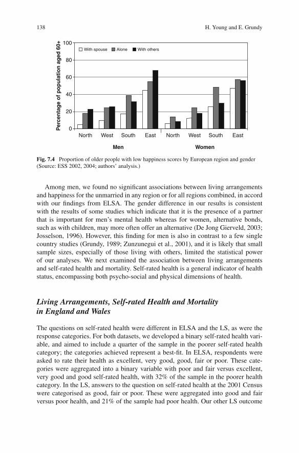
138 H. Young and E. Grundy
Alone With othersWith spouse100
80
60
40
20
0Per
cen
tag
e o
f p
op
ula
tio
n a
ged
60+
WomenMen
North NorthWest South East West South East
Fig. 7.4 Proportion of older people with low happiness scores by European region and gender(Source: ESS 2002, 2004; authors’ analysis.)
Among men, we found no significant associations between living arrangementsand happiness for the unmarried in any region or for all regions combined, in accordwith our findings from ELSA. The gender difference in our results is consistentwith the results of some studies which indicate that it is the presence of a partnerthat is important for men’s mental health whereas for women, alternative bonds,such as with children, may more often offer an alternative (De Jong Gierveld, 2003;Josselson, 1996). However, this finding for men is also in contrast to a few singlecountry studies (Grundy, 1989; Zunzunegui et al., 2001), and it is likely that smallsample sizes, especially of those living with others, limited the statistical powerof our analyses. We next examined the association between living arrangementsand self-rated health and mortality. Self-rated health is a general indicator of healthstatus, encompassing both psycho-social and physical dimensions of health.
Living Arrangements, Self-rated Health and Mortalityin England and Wales
The questions on self-rated health were different in ELSA and the LS, as were theresponse categories. For both datasets, we developed a binary self-rated health vari-able, and aimed to include a quarter of the sample in the poorer self-rated healthcategory; the categories achieved represent a best-fit. In ELSA, respondents wereasked to rate their health as excellent, very good, good, fair or poor. These cate-gories were aggregated into a binary variable with poor and fair versus excellent,very good and good self-rated health, with 32% of the sample in the poorer healthcategory. In the LS, answers to the question on self-rated health at the 2001 Censuswere categorised as good, fair or poor. These were aggregated into good and fairversus poor health, and 21% of the sample had poor health. Our other LS outcome

7 Living Arrangements, Health and Well-Being 139
variable was an indicator of death between the 2001 Census and the end of 2004,and 13% of the sample died during this follow up period. For men and women inboth the LS and ELSA samples, the prevalence of poor self-rated health was lowestamong those living with a spouse, intermediate for those living alone and was high-est for the unmarried living with others (Fig. 7.5). The prevalence of mortality waslowest among those living with a spouse, but the difference between those livingalone and with others was marginal.
Logistic regression was used to examine this association controlled for age andsocio-economic status, both of which are known to be associated with health statusand with living arrangements (Table 7.3). Among the unmarried, analysis of the LSindicated that those living with others were more likely to report poor health and hadhigher risks of mortality than those living alone. Odds ratios from analysis of ELSAalso indicated that living with others was associated with poor health, but resultswere not significant. This may reflect small sample sizes of those living with oth-ers, which reduced the statistical power of the analysis. Rather surprisingly, womenliving with a spouse were significantly more likely to rate their health as poor thanthose living alone after control for age and socio-economic status in both the LSand ELSA. Further investigation of this association in the LS by age demonstratedthat this association was only present for women aged 75 and over. This finding isconsistent with research from the UK and the USA, which also shows that olderold women living alone report better health than those living with a spouse. Thismay reflect the fact that this group includes the never-married who have strongersocial bonds with others outside the household (Goldman et al., 1995; Grundy andSloggett, 2003), and that they do not have to provide support and care for a spouse,
Alone With othersWith spouse
50
40
30
20
10
0Per
cen
tag
e o
f p
op
ula
tio
n a
ged
60+
ELSA
WomenMenWomenMenWomenMen
ONS LS
Self-rated health 2002 Self-rated health 2001 Mortality 2001-04
Fig. 7.5 Prevalence of poor self-rated health and mortality for the population aged 60+ by livingarrangement and gender(Source: ELSA, 2002; ONS LS, 2001–2004; authors’ analysis.)

140 H. Young and E. Grundy
Table 7.3 Results from logistic regression model of proportion of men and women aged 60+with poor self rated health 2001/2002 and mortality 2001–2004 by living arrangements and otherfactors, England 2002, England and Wales 2001
Men WomenOdds Ratio p-value 95% CI Odds Ratio p-value 95% CI
ELSA: Poor self-rated health 2002a
Living Alone 1.00 1.00arrangements With spouse 1.11 0.91,1.36 1.25 ∗ 1.05,1.49
With others 1.17 0.75,1.83 1.10 0.82,1.47Age 1.01 ∗ 1.00,1.02 1.02 ∗∗∗ 1.01,1.03Net wealth Less wealth 1.28 ∗∗∗ 1.20,1.37 1.34 ∗∗∗ 1.26,1.43Housing tenure Owner
occupier1.00 1.00
Renter 1.78 ∗∗∗ 1.46,2.18 1.37 ∗∗∗ 1.14,1.64Highesteducationalqualification
Highersecondaryor above
1.00 1.00
Lowersecondary
1.06 0.84,1.34 0.98 0.75,1.27
None 1.64 ∗∗∗ 1.35,1.99 1.49 ∗∗∗ 1.24,1.79N = 3,176 N = 3,837
LS: Poor self-rated health 2001b
Living Alone 1.00 1.00arrangements With spouse 0.98 0.91,1.04 1.16 ∗∗∗ 1.10,1.23
With others 1.30 ∗∗∗ 1.14,1.48 1.36 ∗∗∗ 1.25,1.47
Age 1.03 ∗∗∗ 1.03,1.03 1.05 ∗∗∗ 1.05,1.05
Region South & East 1.00 1.00Central 1.30 ∗∗∗ 1.22,1.38 1.38 ∗∗∗ 1.31,1.46North &
Wales1.58 ∗∗∗ 1.48,1.68 1.51 ∗∗∗ 1.43,1.60
Tenure and caraccess c
Lower score 1.24 ∗∗∗ 1.22,1.27 1.24 ∗∗∗ 1.22,1.26
Social class 1971 1.18 ∗∗∗ 1.14,1.23N = 35,689 N = 43,062
LS: Mortality 2001–2004
Living Alone 1.00 1.00arrangements With spouse 0.85 ∗∗∗ 0.79,0.92 0.93 0.87,1.01
With others 1.11 0.96,1.30 1.24 ∗∗∗ 1.13,1.37
Age 1.12 ∗∗∗ 1.12,1.13 1.12 ∗∗∗ 1.12,1.12
Region South & East 1.00 1.00Central 1.06 0.99,1.15 1.04 0.97,1.12

7 Living Arrangements, Health and Well-Being 141
Table 7.3 (continued)
Men Women
Odds Ratio p-value 95% CI Odds Ratio p-value 95% CI
North &Wales
1.07 0.99,1.16 1.12 ∗∗ 1.04,1.21
Tenure andcar access c
Lower score 1.17 ∗∗∗ 1.14,1.20 1.14 ∗∗∗ 1.12,1.16
Social class1971
1.03 0.98,1.08
N = 35,689 N = 43,062
aOutcome variable self rated health categorised into very poor and poor versus fair, goodand very good health. bOutcome variable self rated health categorised into not good versusfairly good and good health. cSummary score of tenure and car access in 1971 and 1981.∗p<0.05∗∗p<0.01∗∗∗p<0.001.Source: ELSA, 2002; ONS LS, 2001–2004; authors’ analysis.
with possible negative implications for health and well-being. However, the never-married only accounted for 13% of those living alone, and the majority were wid-owed. In opposition to our finding for self-rated health, women living with a spousehad a lower (of border line significance) odds of mortality compared with thoseliving alone. These differences by type of health indicator show that different mea-sures are indicators of different processes. For example, self-rated health capturessocio-psychological dimensions of health (Grundy and Sloggett, 2003; Idler andBenyamini, 1997). Our model results also showed that increasing age, having lowerlevels of socio-economic status, and living outside the South and East of Englandwere associated with poorer self-rated health and higher mortality.
Our results consistently indicated that among the unmarried, those living withothers were more likely to have poor self-rated health and higher mortality thanthose living alone. This finding may be a result of health selection and we nextexamine the part that health selection may have played in our results using the LS.To do this, we examined the association between living arrangement change from1991 to 2001 health outcomes in 2001 for a subpopulation of our LS sample. Wefocused on LS members in our sample who were unmarried and did not report alimiting long term illness (LLTI) at the 1991 Census. We excluded those who wereliving with a spouse in 1991 in order to exclude the health influence of widowhoodin the inter-censal period on our results (Lee et al., 2001; Wilcox et al., 2003). Thesample may still have included individuals who were unmarried in 1991 but thenwere married and widowed before 2001, but this proportion would be small in theage groups we consider. We excluded those with a LLTI in 1991 because we wereinterested in health related changes in living arrangement. We made the assump-tion that individuals who did not have an LLTI in 1991 and did in 2001 and whochanged to living with others were likely to have made a health-related change.If those who changed to living with relatives rather than living alone or living

142 H. Young and E. Grundy
with others at both time points were more likely to have developed poor self-ratedhealth in 2001, we assumed that this would demonstrate a health selection effect onour results.
We used logistic regression to model the association between living arrange-ment change and all three health outcome variables, controlling for age and socio-economic status (Table 7.4). This analysis confirms that those changing to live withothers were significantly more likely to have an LLTI and poor self-rated healthin 2001 than those who lived alone at both time points. They also had increasedodds of death 2001–2004, but this association was not significant. Among women,those living with others in both 1991 and 2001 were also more likely to experiencepoor health outcomes in 2001, but the magnitude of the odds ratios was marginally
Table 7.4 Results from logistic regression model of proportion of men and women who wereunmarried and who had no LLTI in 1991, who then had poor self rated health or an LLTI in2001 or died 2001–2004 by living arrangement change 1991–2001, controlled for other factors,a England and Wales
Men Women
Living arrangementchange 1991–2001
OR p-value
95% CI N OR p-value
95% CI N
Self-rated health
No change Alone – alone 1.00 1,980 1.00 6,638With others – with
others1.15 0.90,1.46 615 1.39 ∗∗∗ 1.21,1.59 1,697
Change Alone – with others 2.29 ∗∗∗ 1.40,3.74 85 1.67 ∗∗∗ 1.27,2.19 312With others – alone 1.03 0.80,1.33 637 0.95 0.80,1.14 1,444Alone or with
others – spouse1.17 0.88,1.56 509 0.97 0.70,1.34 428
Limiting long term illness
No change Alone – alone 1.00 1,980 1.00 6,638With others – with
others1.08 0.89,1.30 615 1.23 ∗∗∗ 1.10,1.38 1,697
Change Alone – with others 2.16 ∗∗∗ 1.38,3.37 85 1.70 ∗∗∗ 1.34,2.17 312With others – alone 1.00 0.82,1.22 637 1.04 0.91,1.18 1,444Alone or with
others – spouse1.06 0.85,1.32 509 0.85 0.67,1.07 428
Death 2001–2004
No change Alone – alone 1.00 1,980 1.00 6,638With others – with
others0.97 0.75,1.26 615 1.23 ∗ 1.05,1.44 1,697
Change Alone – with others 1.25 0.70,2.22 85 1.31 0.96,1.79 312With others – alone 1.10 0.84,1.45 637 1.12 0.92,1.38 1,444Alone or with
others – spouse0.72 0.50,1.04 509 0.61 0.36,1.04 428
N = 3,826 N = 10,519
aControlled for age, socio-economic status and LLTI in 1991. ∗p<0.05∗∗p<0.01∗∗∗p<0.001.Source: ONS LS, 1991–2004; authors’ analysis.

7 Living Arrangements, Health and Well-Being 143
smaller than for those who only lived with others in 2001. Therefore, while healthselection may account for some of the association between living with others andpoor health, those living with others for longer time periods are also more likelyto change the rating of their health from good or fair to poor. It is worth noting,however, when applying these results to the general population that only very smallproportions (two per cent of this subpopulation) moved to live with others and only16% lived with others at both time points. Much larger proportions lived alone atboth time points.
Living Arrangement and Self-rated Health in Europe
Having established that older people living with others were generally more likelyto have poor self-rated health than those in other living arrangements in Englandand Wales, at least in part due to health selection, the ESS was used to examinethis association in different regions of Europe. In the ESS, self-rated health wasmeasured using a five category variable including very good, good, fair, bad andvery bad health. We dichotomised the variable into very good, good and fair versusbad and very bad self-rated health, with 23% of the sample rating their health as bador very bad. Note that this categorisation is in line with our LS and ELSA analysisabove.
Unmarried men living with others had the highest prevalence of poor self-ratedhealth in all regions, except the west region where the prevalence was higher for
Alone With othersWith spouse
100
80
60
40
20
0Per
cen
tag
e o
f p
op
ula
tio
n a
ged
60+
WomenMen
North NorthWest South East West South East
Fig. 7.6 Proportion of the population aged 60+ with bad or very bad self-rated health by regionand gender, 19 European countries(Source: ESS 2002 and 2004; authors’ analysis.)

144 H. Young and E. Grundy
those living alone (Fig. 7.6). Among unmarried women, the prevalence of poor self-rated health was in general higher among those living alone than among those livingwith others. Multivariate analyses, using logistic regression controlling for age andsocio-economic status demonstrated that, as for England and Wales, those livingwith a spouse were less likely to have poor self-rated health than those living alone(results not shown). However, results indicated that in all regions combined, womenliving with others had a lower likelihood of poor self-rated health than those livingalone, in opposition to our findings from ELSA and the LS.
When we analysed regions separately, this association was significant for theeastern region (p = 0.01) and was of borderline significance in the southern region(p = 0.10), but there was no significant association in the northern and westernregions. There were also no significant associations among unmarried men for allregions combined or by region. For self-rated health and mortality, we thereforefound differing results by region. While in England and Wales there was an associ-ation between living with others and poor self-rated health, in southern and easternEurope, living alone was associated with poor self-rated health rather than livingwith others.
Conclusions
What do these results show about the associations between living arrangements andhealth and well-being? In England and Wales, as expected, older people living witha spouse had the best levels of health and well-being, except for older women liv-ing alone who rated their health as better than those living with a spouse. Amongthe unmarried in England and Wales, those living alone rated their health bet-ter than those living with others and were less likely to die during the follow-upperiod, but they were also more likely to be depressed and lonely than those liv-ing with others. We found, as expected, that these associations varied by regionof Europe, which is likely to be associated with differences in culture and welfareregimes.
In northern Europe (here comprising Sweden, Norway, Finland and Denmark),unlike all other regions, we found no association between living alone and low levelsof well-being. This may be due to the fact that older people in this region have pref-erences for autonomy and independence, and receive generous benefits and supportfrom the state to enable them to live independently (Daatland, 1990; Daatland andHerlofson, 2001; Millar and Warman, 1996; Reher, 1998). The association betweenliving alone and poorer emotional well-being in England and Wales was also foundin western, southern and eastern Europe, and may be associated with the impor-tance of the role of the family in supporting older people in these regions. In south-ern Europe, public policy reinforces the traditional focus of care and support bythe family (Twigg, 1996), and high percentages of the population in MediterraneanEurope support the move of elderly parents into the child’s home when unable tocope alone (Tomassini et al., 2004). In eastern Europe, there are still relatively low

7 Living Arrangements, Health and Well-Being 145
levels of community social care (Botev, 1999; De Jong Gierveld et al., 2001; Tobis,2000), and perhaps older people living alone are particularly disadvantaged andunhappy due to a lack of family support. The UK is similar to Scandinavia in termsof public attitudes to family responsibility (Katz et al., 2003), but welfare policyplaces obligations on the nuclear family for support and care unlike Scandinaviancountries (Millar and Warman, 1996). Future research on this topic could include aninvestigation of the further possible negative implications for well-being of livingalone for women in eastern, southern and western regions of Europe using largerlongitudinal datasets.
While we found that living with others was associated with poorer health in Eng-land and Wales, in eastern and southern Europe, those living alone were likely to ratetheir health as poorer than those living with others, in addition to a having a higherlikelihood of unhappiness. Self-rated health has a psychological component to it andthis finding may reflect a preference for living with others rather than alone in theseareas, especially in southern Europe. As already mentioned, lower levels of com-munity based social services in eastern and southern Europe than in other regionsof Europe (Bond and Cabrero, 2007; Tobis, 2000) may mean that those living withfamily receive higher levels of care and support than those living alone, resulting inbetter self-rated health. Additionally, in the southern and eastern regions, it is morenormative to live with others and as there are higher proportions of people doing so,they are less likely to be a group selected for poor health. In northern and westernEurope, where there are fewer older people living with others, those who do aremore likely to be in poor health. In line with this, we found that in England andWales, the association between living with others and poor self-rated health was atleast in part due to health selection. However, we also found that those living withothers for longer periods of time were more likely to develop an LLTI than thoseliving alone. It is important to note that in terms of generalising these results to thepopulation, the majority of unmarried older people live alone in England and Walesand very few move to live with others. To fully eliminate the effects of health selec-tion and to establish causal pathways, we would need longitudinal data with morefrequent follow ups. We would also need data on health status at the time of a livingarrangement transition, and more detailed measures of health status. This may bepossible for England once further waves of ELSA have been completed. Europeanregional differences in health selection could also be investigated further using lon-gitudinal datasets such as SHARE when more rounds of data have been collected.
Some caution is needed when interpreting results because some analyses lackedstatistical power due to small sample sizes, especially of men living with others inthe northern and western regions. Further work using more detailed health indica-tors might also reveal associations between health and disability and living arrange-ments which we were unable to detect using the relatively crude indicators avail-able in these datasets. Additionally, regional analysis may obscure country-levelassociations and so more detailed country specific studies are also needed to elu-cidate associations between living arrangements and well-being, and the factorsunderlying them. Nevertheless, our findings demonstrate that whether or not livingalone has positive or negative consequences for older people’s health and emotional
146 H. Young and E. Grundy
well-being depends on the cultural context and the availability and acceptability ofalternative supports for those in need of assistance. With growing proportions ofthe population in older age groups and a high propensity to live alone, numbers ofolder people living alone are projected to increase in the coming decades in the UKand throughout Europe. These increases may well have negative implications for thehealth and well-being of some.
Acknowledgments We are grateful to the ONS for permission to use the LS, and for help pro-vided by staff of the Centre for Longitudinal Study Information and User Support (CeLSIUS).CeLSIUS is supported by the ESRC Census of Population Programme (Award Ref: RES-348-25-0004). Census output is Crown copyright and is reproduced with the permission of the Controllerof HMSO and the Queen′s Printer for Scotland. We are also grateful to the National Centre forSocial Research and the UK Data Archive for access to the ELSA data, and to the NorwegianSocial Science Data Service as the data archive and distributor of the ESS data. The authors aloneare responsible for the interpretation of the data.
References
Banks, J., Breeze, E., Lessof, C. and Nazroo, J. (2006). Retirement, Health and Relationships ofthe Older Population in England: The 2004 English Longitudinal Study of Ageing (Wave 2),Institute of Fiscal Studies, London.
Barnes, M., Blom, A., Cox, K. and Lessof, C. (2006) The Social Exclusion of Older People: Evi-dence from the First Wave of the English Longitudinal Study of Ageing (ELSA), Social Exclu-sion Unit, Office of the Deputy Prime Minister, London.
Bond, J. and Cabrero, G.R. (2007) Health and dependency in later life, in Bond, J., Peace, S.,Dittmann-Kohli, F. and Westerhof, G. (eds.) Ageing in Society, Sage, London, pp. 113–141.
Botev, N. (1999) Older persons in countries with economies in transition, in Population Age-ing, Challenges for Policies and Programmes in Developed and Developing Countries, UnitedNations Population Fund and CBGS, New York and Brussels, pp. 85–100.
Braam, A.W., Prince, M.J., Beekman, T.F., Delespaul, P., Dewey, M.E., Geerlings, S.W., Kivela,S.L., Lawlor, B.A., Magnusson, H., Meller, I., Peres, K., Reischies, F.M., Roelands, M.,Schoevers, R.A., Saz, P., Skoog, I., Turrina, C., Versporten, A. and Copeland, J.R.M. (2005)Physical health and depressive symptoms in older Europeans: Results from EURODEP, BritishJournal of Psychiatry, 187: 35–42.
Brown, J.W., Liang, J., Krause, N., Akiyama, H., Sugisawa, H. and Fukaya, T. (2002) Transitionsin living arrangements among elders in Japan: Does health make a difference?, Journals ofGerontology Series B-Psychological Sciences and Social Sciences, 57(4), S209–S220.
Burnette, D. and Mui, A.C. (1996) Psychological well-being among three successive cohorts ofolder American women who live alone, Journal of Women & Aging, 8(1), 63–80.
Castro-Costa, E., Dewey, M., Steward, R., Banerjee, S., Huppert, F., Mendonca-Lima, C., Bula, C.,Reisches, F., Wancata, J., Ritchie, K., Tsolaki, M., Mateos, R. and Prince, M. (2007) Prevalenceof depressive symptoms and syndromes in later life in ten European countries: The SHAREstudy, British Journal of Psychiatry 191e Psychological Medicine, 6: 551–563.
Comstock, G.W. and Helsing, K. (1976) Symptoms of depression in two communities, Psycholog-ical Medicine, 6: 551–563.
Crumley, B. (2003) Elder careless. Time Europe, London.Daatland, S.O. (1990). What are families for? On family solidarity and preferences for help, Ageing
and Society, 10, 1–15.Daatland, S.O. and Herlofson, K. (2001). Service systems and family care – substitution or comple-
mentarity? in Daatland, S.O. and Herlofson, K. (eds.) Ageing, Inter-generational Relationships,

7 Living Arrangements, Health and Well-Being 147
Care Systems and Quality of Life. An Introduction to the OASIS Project, NOVA, Oslo,pp. 53–61.
Daatland, S.O. and Herlofson, K. (2003) ‘Lost solidarity’ or ‘changed solidarity’: a comparativeEuropean view of normative family solidarity, in Gender and Ageing Changing Roles and Rela-tionships, Open University Press, Maidenhead, pp. 95–110.
De Jong Gierveld, J. (2003) Social networks and social well-being of older men and women livingalone, in Arber, S., Davidson, K. and Ginn, J. (eds.) Gender and Ageing Changing Roles andRelationships, Open University Press, Maidenhead.
De Jong Gierveld, J., De Valk, H. and Blommesteijn, M. (2001) Living arrangements of older per-sons and family support in more developed countries, Population Bulletin of the United Nations,special issue, living arrangements of older persons: Critical Issues and Policy Responses,42/43: 193–217.
Department of Health (2001) National Service Framework for Older People. Department of Health,London.
Elman, C. and Uhlenberg, P. (1995) Early twentieth century co-residence of the elderly and theirchildren, Population Studies, 49: 501–517.
European Commission (2006) The Demographic Future of Europe – From Challenge to Opportu-nity, European Commission, Luxembourg.
Fratiglioni, L., Wang, H.X., Ericsson, K., Maytan, M. and Winblad, B. (2000) Influence of socialnetwork on occurrence of dementia: a community-based longitudinal study, Lancet, 355(9212):1315–1319.
Garcia, E.L., Banegas, J.R., Perez-Regadera, A.G., Cabrera, R. and Rodriguez-Artalejo, F. (2005)Social network and health-related quality of life in older adults: A population-based study inSpain. Quality of Life Research, 14(2): 511–520.
Glaser, K., Murphy, M. and Grundy, E. (1997) Limiting long-term illness and household structureamong people aged 45 and over, Great Britain, 1991, Ageing and Society, 17: 3–20.
Glaser, K., Tomassini, C. and Grundy, E. (2004) Revisiting convergence and divergence: supportfor older people in Europe, European Journal of Ageing, 1: 64–72.
Goldman, N., Korenman, S. and Weinstein, R. (1995) Marital status and health among the elderly,Social Science & Medicine, 40: 1717–1730.
Grundy, E. (1989) Longitudinal perspectives on the living arrangements of the elderly, in Jefferys,M. (ed.) Growing Old in the Twentieth Century, Routledge, London, pp. 128–150.
Grundy, E. (1993) Moves into supported private households among elderly people in England andWales, Environment and Planning A, 25: 1467–1479.
Grundy, E. (1996) Population review: The population aged 60 and over, Population Trends, 84:14–20.
Grundy, E. (1999) Changing role of the family and community in providing support for the elderly,in Cliquet, R. and Nizamuddin, M. (eds.) Population Ageing. Challenges for Policies and Pro-grammes in Developed and Developing Countries, UNFPA, New York, pp. 103–122.
Grundy, E. (2000) Co-residence of mid-life children with their elderly parents in England andWales, changes between 1981 and 1991, Population Studies, 54, 193–206.
Grundy, E. (2001) Living arrangements and the health of older persons in developed countries,Population Bulletin of the United Nations, special issue, living arrangements of older persons:Critical Issues and Policy Responses, 42/43: 311–329.
Grundy, E. (2006) Ageing and vulnerable elderly people: European perspectives, Ageing and Soci-ety, 26: 105–134.
Grundy, E. and Sloggett, A. (2003) Health inequalities in the older population: the role of personalcapital, social resources and socio-economic circumstances, Social Science & Medicine, 56:935–947.
Gustavson, K. and Lee, C. (2004). Alone and content: frail seniors living in their own homescompared to those who live with others, Women and Aging, 16(3–4): 3–18.
Hahn, B.A. (1993) Marital status and women’s health, the effect of economic and marital acquisi-tions, Journal of Marriage and the Family, 55: 495–504.
148 H. Young and E. Grundy
Hall, M. and Havens, B. (2001) The Effects of Social Isolation and Loneliness on the Health ofOlder Women, Centres of Excellence for Women’s Health, Winnipeg.
Hattersley, L. and Creeser, R. (1995) Longitudinal Study 1971–1991. History, Organisation andQuality of Data, ONS, London.
Hughes, M.E. and Waite, L.J. (2002) Health in household context: living arrangements and healthin late middle age, Journal of Health and Social Behavior, 43(1): 1–21.
Hughes, M.E., Waite, L.J., Hawkley, L.C. and Cacioppo, J.T. (2004) A short scale for measuringloneliness in large surveys: results from two population-based studies, Research on Aging, 26:655–672.
Iacovou, M. (2000) The living arrangements of elderly Europeans, No. 2000–2009, Institute forSocial and Economic Research, Essex.
Idler, E.L. and Benyamini, Y. (1997) Self-rated health and mortality: a review of twenty-sevencommunity studies, Journal of Health and Social Behavior, 38: 21–37.
Iliffe, S., Tai, S.S., Haines, A., Gallivan, S., Goldenberg, E., Booroff, A. and Morgan, P. (1992)Are elderly people living alone an at risk group? British Medical Journal, 305: 1001–04.
Iwata, N. and Buka, S. (2002) Race/ethnicity and depressive symptoms: a cross-cultural/ethniccomparison among university students in East Asia, North and South America, Social Science& Medicine, 55: 2243–2252.
Josselson, R. (1996) The Space Between Us. Exploring the Dimensions of Human Relationships,Sage, Thousand Oaks, CA.
Jowell, R. (2003) European Social Survey 2002/2003: Technical Report, Centre for ComparativeSocial Surveys, City University, London.
Katz, R., Daatland, S.O., Lowenstein, A., Bazo, M.T., Ancizu, I., Herlofson, K., Mehlhausen-Hassoen, D. and Prilutzky, D. (2003) Family norms and preferences in intergenerational rela-tions, in Bengston V. and Lowenstein, A. (eds.) Global Ageing and Challenges to Families,Aldine de Grutyer, New York, pp. 305–326.
Kendig, H., Dykstra, P.A., van Gaalen, R.I. and Melkas, T. (2007) Health of aging parents andchildless individuals, Journal of Family Issues, 28(11): 1457–1486.
Kharicha, K., Iliffe, S., Harari, D., Swift, C., Gillmann, G. and Stuck, A. (2007) Health riskappraisal in older people 1: are older people living alone an ′at-risk′ group? British Journalof General Practice, 57: 271–276.
Klinenberg, E. (2002). Heat Wave: A Social Autopsy of Disaster in Chicago, University of ChicagoPress, Chicago.
Kohler, H.P., Behrman, J.R. and Skytth, A. (2005) Partner + Children=Happiness? Theeffects of partnerships and fertility on well-being, Population and Development Review, 31:407–455.
Kohli, M. and Albertini, M. (2006) The Impact of Welfare and Family Regimes on TransfersBetween Older Parents and Their Adult Children, Varenna, Italy.
Koskinen, S., Joutsenniemi, K., Martelin, T. and Martikainen, P. (2007) Mortality differ-ences according to living arrangement, International Journal of Epidemiology, 36(6):1255–1264.
Lee, G.R., DeMaris, A., Bavin, S. and Sullivan, R. (2001) Gender differences in the depressiveeffect of widowhood in later life, Journals of Gerontology Series B-Psychological Sciencesand Social Sciences, 56(1): S56–61.
Lehtinen, V., Sohlman, B. and Kovess-Masfety, V. (2005) Level of positive mental health in theEuropean Union: results from the Eurobarometer 2002 Survey, Clinical Practice and Epidemi-ology in Mental Health, 1: 9.
Lund, R., Modvig, J., Due, P. and Holstein, B.E. (2000) Stability and change in structural socialrelations as predictor of mortality among elderly women and men, European Journal of Epi-demiology, 16(12): 1087–1097.
Marmot, M., Banks, J., Blundell, R., Lessof, C. and Nazroo, J. (2002). Health, Wealth andLifestyles of the Older Population in England: The 2002 English Longitudinal Study of Ageing,Institute for Fiscal Studies, London.

7 Living Arrangements, Health and Well-Being 149
McGarry, K. and Schoeni, R.F. (2000) Social security, economic growth, and the rise in elderlywidows′ independence in the twentieth century, Demography, 37(2): 221–236.
Michael, Berkman, L.F., Colditz, G.A. and Kawachi, I. (2001) Living arrangements, social inte-gration, and change in functional health status, American Journal of Epidemiology, 153(2):123–131.
Michael, R., Fuchs, V. and Scott, S. (1980) Changes in the propensity to live alone, Demography,19: 39–53.
Millar, J. and Warman, A. (1996) Family Obligations in Europe, Family Policy Studies Centre,London.
Mindel, C.H. and Wright, R. (1982). Differential living arrangements among the elderly and theirsubjective well-being, Activities, Adaptation and Aging, 2: 25–34.
Montgomery, S.M., Netuveli, G., Hildon, Z. and Blane, D. (2007) Does financial disadvantage atolder ages eliminate the potential for better health?, Journal of Epidemiology and CommunityHealth, 61: 891–895.
Mor, V., Murphy, J., Masterson-Allen, S., Willey, C., Razmpour, A., Jackson, M.E., Greer, D. andKatz, S. (1989) Risk of functional decline among well elders, Journal of Clinical Epidemiology,42(9): 895–904.
Mui, A.C. and Burnette, D. (1994) A comparative profile of frail elderly persons living alone andthose living with others, Journal of Gerontological Social Work, 21: 5–26.
Murata, C., Kondo, T., Hori, Y., Miyao, D., Tamakoshi, K., Yatsuya, H., Sakakibara, H.and Toyoshima, H. (2005) Effects of social relationships on mortality among the elderlyin a Japanese rural area: An 88-month follow-up study, Journal of Epidemiology, 15(3):78–84.
Murphy, M., Grundy, E. and Kalogirou, S. (2007) The increase in marital status differences inmortality up to the oldest age in seven European countries, 1990–99, Population Studies, 61(3):287–298.
Netuveli, G., Wiggins, R.D., Hildon, Z., Montgomery, S.M. and Blane, D. (2006) Quality of lifeat older ages: evidence from the English Longitudinal Study of Ageing (wave 1), Journal ofEpidemiology Community Health, 60: 357–363.
ODPM. (2006) The Social Exclusion of Older People: Evidence from the First Wave of the EnglishLongitudinal Study of Ageing (ELSA), HMSO, London.
Office for National Statistics (2004) Census 2001 Definitions, Office for National Statistics,London.
Olafsson, S. (2003) Welfare trends of the 1990s in Iceland, Scandinavian Journal of Public Health,31: 401–404.
Pampel, F.C. (1992) Trends in living alone among the elderly in Europe, in Rogers, A. (ed.) ElderlyMigration and Population Redistribution, Belhaven Press, London, pp. 97–117.
Pillemar, K., Moen, P., Wethington, E. and Glasgow, N. (2000) Social Integration in the SecondHalf of Life, Johns Hopkins University Press, Baltimore.
Pizzetti, P., Manfredini, M. and Lucchetti, E. (2005) Variations in late-age mortality by householdstructure and marital status in Parma, Italy, Ageing and Society, 25: 305–318.
Radloff, L.S. (1977) The CES-D scale: A self-report depression scale for research in the generalpopulation, Applied Psychological Measurement, 1: 385–401.
Reher, D.S. (1998) Family ties in Western Europe: persistent contrasts, Population DevelopmentReview, 24(2): 203–234.
Russell, D.W. (1996) UCLA Loneliness scale (version 3): reliability, validity, and factor structure,Journal of Personality Assessment, 66: 20–40.
Sarwari, A.R., Fredman, L., Langenberg, P. and Magaziner, J. (1998) Prospective study on therelation between living arrangement and change in functional health status of elderly women,American Journal of Epidemiology, 147(4): 370–378.
Silverstein, M. and Bengston, V. (1994) Does intergenerational social support influence the psy-chological well-being of older parents? The contingencies of declining health and widowhood,Social Science & Medicine, 38(7): 943–957.

150 H. Young and E. Grundy
Soule, A., Babb, P., Evandrou, M., Balchin, S. and Zealey, L. (2005) Focus on Older People, Officefor National Statistics, London.
Steffick, D.E. (2000) HRS/AHEAD Documentation Report – Documentation of Affective Func-tioning Measures in the Health and Retirement Study, University of Michigan, AnnArbour.
Sundstrom, G. and Tortosa, M.A. (1999). The effects of rationing home-help services in Spain andSweden: a comparative analysis, Aging and Society, 19: 343–361.
Tobis, D. (2000) Moving from Residential Institutions to Community-Based Social Services in Cen-tral and Eastern Europe and the Former Soviet Union, The International Bank for Reconstruc-tion and Development, The World Bank, Washington D.C.
Tomassini, C., Glaser, K., Wolf, D., van Groenou, M. and Grundy, E. (2004) Living arrangementsamong older people: an overview of trends in Europe and the USA, Population Trends, 115:24–34.
Twigg, J. (1996) Issues in informal care, in OECD (ed.) Caring for Frail Elderly People: Policiesin Evolution, Vol. Social Policy Studies No. 19, OECD, Paris, pp. 81–92.
Ulbrich, P.M. and Warheit, G.J. (1989) Social support, stress and psychological distress amongolder black and white adults, Journal of Aging and Health, 1: 286–305.
United Nations (2002) Report of the Second World Assembly on Ageing Madrid, 8–12 April2002,United Nations, New York.
Walter-Ginzburg, A., Blumstein, T., Chetrit, A. and Modan, B. (2002) Social factors and mortalityin the old-old in Israel: The CALAS study, Journals of Gerontology Series B-PsychologicalSciences and Social Sciences, 57(5): S308–S318.
Wenger, G.C. (1984) The Supportive Network: Coping with Old Age, Allen and Unwin, London.Wilcox, S., Evenson, K.R., Aragaki, A., Wassertheil-Smoller, S., Mouton, C.P. and Loevinger, B.L.
(2003) The effects of widowhood on physical and mental health, health behaviors, and healthoutcomes: The Women’s Health Initiative, Health Psychology, 22(5): 513–522.
Wilson, K.C.M., Chen, R., Taylor, S., McCracken, C.F.M. and Copeland, J.R.M. (1999) Socio-economic deprivation and the prevalence and prediction of depression in older community res-idents, British Journal of Psychiatry, 176: 549–553.
Zunzunegui, M.V., Beland, F. and Otero, A. (2001) Support from children, living arrangements,self-rated health and depressive symptoms of older people in Spain, International Journal ofEpidemiology, 30(5): 1090–1099.

Chapter 8Stepparenting and Mental Health
Peteke Feijten, Paul Boyle, Zhiqiang Feng, Vernon Gayleand Elspeth Graham
Introduction
Demographic changes in the Western world over the last few decades, such as latermarriages, lower fertility, increasing divorce rates and rising rates of cohabitation,have brought about significant changes in household formation and composition.One outcome is a growing number of stepfamilies, where a parent, whether nevermarried, separated, widowed or divorced, forms a new marriage or partnership.Nowadays, most stepfamilies result from divorce, while in the past they were morelikely to result from widowhood.
Despite the rising incidence of stepfamilies and the demographic and socialdifferences between stepfamilies and traditional families with two biological par-ents, researchers concerned with family life and parenting were relatively slowto acknowledge the importance of such non-traditional families (Ferri and Smith,1998; Utting, 1995). While there has been an increase in social science research onstepfamilies in recent years much remains to be done (Coleman et al., 2000). Forexample, numerous researchers have explored the effect of living in a stepfamilyon children, including studies of their psychological well-being but, perhaps sur-prisingly, little research has considered the potential psychological impacts on theadults (stepparents and their partners) of living in such a household arrangement.This is the focus of this study.
Background
In the UK most people live in ‘traditional’ households, but non-traditional house-holds are becoming more common. Of those marrying during the 1990s, nearly 50%will end up divorced if current trends continue (Allan, 1999), and a growing num-ber of divorcees are starting new relationships. Haskey (1994) estimated that 12%of British children will live in a stepfamily before their sixteenth birthday. Recent
P. Boyle (B)School of Geography and Geosciences, University of St Andrews, St Andrews, KY16 9AL, UKe-mail: [email protected]
J. Stillwell et al. (eds.), Fertility, Living Arrangements, Care and Mobility, UnderstandingPopulation Trends and Processes 1, DOI 10.1007/978-1-4020-9682-2 8,C© Springer Science+Business Media B.V. 2009
151

152 P. Feijten et al.
estimates for Britain suggest that about 40% of mothers will experience being a loneparent and about 75% of lone mothers will go on to form a stepfamily (Ermisch andFrancesconi, 2000). Currently nearly 90% of stepfamilies involve children livingwith their mother and a new male partner (Finch, 2002). Importantly, stepfamiliesdiffer from traditional families demographically because they tend to include moreand older children than do first families (Haskey, 1994). The greater complexityof intra-household relationships in stepfamilies provides scope for tensions to ariseand, perhaps, increases the potential for negative health impacts for both the childrenand the parents.
Numerous studies highlight the strains that every-day life in stepfamilies mayentail and the effects this may have on stepchildren’s health and well-being (Brownand Booth, 1996; Pryor and Rodgers, 2001). Not only do stepchildren experience thebreakdown of their parents’ relationship but they often feel relatively neglected bythe biological parent. This may be combined with the potentially disruptive effectsof having to divide their time between two homes. Most studies of the effects ofremarriage on children fail to show a benefit, despite the financial advantages thatusually result (Fergusson et al., 1994; Pagani et al., 1998; Walper, 1995; Duncan andHoffman, 1985; Zill, 1988). Some findings point to negative effects, with stepchil-dren performing worse at school (Pong, 1997; Teachman et al., 1996), five-year oldchildren in stepfamilies being significantly more at risk of behavioural and devel-opmental problems than children in traditional families (Wadsworth et al., 1985),and a higher risk of drinking alcohol, drug abuse and problem behaviour amongschoolchildren living with a stepfather (Del Carmen et al., 2002; Mekos et al., 1996).While Joshi et al. (1999) found that maternal educational attainment and, to a lesserextent, family economic circumstances eliminated the relationship between familystructure and children’s cognitive and behavioural outcomes, the majority of quan-titative studies suggest that stepchildren are at greater risk of a range of problems(Coleman et al., 2000; Ram and Hou, 2003).
There is also a considerable literature on the effects of family arrangements andmarital status on adult health. Higher mortality rates among the unmarried, thosewho live alone and the divorced, compared to those who are married, are well estab-lished (Seeman et al., 1987; Trovato and Lauris, 1989; Gardner and Oswald, 2004).More depressive symptoms are apparent among both the recently separated (Neffand Schluter, 1993) and those who have been separated for longer (Richards et al.,1997), even when mental health status prior to separation/divorce is taken intoaccount (Wade and Pevalin, 2004). In some studies, the beneficial effects of mar-riage are found for men but not women (Berkman and Syme, 1979; Avlund et al.,1998). Lone parenthood has also been studied in some detail. Hope et al. (1999)found that lone parents suffer higher levels of mental distress than other parents,although this may be related to the significantly higher poverty levels they experi-ence (Keirnan and Mueller, 1998; Shouls et al., 1999). Notably, within this largeliterature, there are virtually no studies examining explicitly the effects of living ina stepfamily on stepparents’ and their partner’s health.
Another strand of the literature which is relevant to this study considers ‘mar-ital quality’ and how people cope with the redefinition of kinship that follows

8 Stepparenting and Mental Health 153
divorce and remarriage (overviews are provided by Coleman and Ganong, 1990;Pasley et al., 1993). Remarriage has been found to lead to lower marital quality andsatisfaction than first marriage (Clingempeel, 1981; White and Booth, 1985), andthis may have an impact upon mental health. In a qualitative study by Simpson(1994), it was argued that the roles of remarried persons compared to married per-sons, and stepparents compared to biological parents, are less well defined and thusharder to fulfil with confidence and satisfaction. This is sometimes labelled as the‘incomplete institution hypothesis’ (Cherlin, 1978). We found one study specifi-cally focusing on the experience of stepparenting and how this affected maritalquality and the stepparent-stepchild relationship. Ambert (1986) showed that anintimate relationship between stepparents and stepchildren was harder to establishwhen stepchildren were not resident and that the birth of a common child into thestepfamily made the stepparent-stepchild relationship better for men, but not forwomen.
Thus, stepfamily arrangements are potentially stressful since they involve thenegotiation of different intra-household relationships that may introduce newsources of tension. For example, Hetherington and Jodl (1994) found that step-parents remain less engaged and more authoritarian in parenting stepchildren thanin parenting their biological children, illustrating the scope for friction betweenbiological parents and stepparents. Yet a recent wide-ranging literature review onremarriage and stepparenting cited only a small number of studies on the psycholog-ical health of adults, the majority of which examined the general effects of remar-riage (Coleman et al., 2000). A study by Ferri and Smith (1998) suggested thatadults in stepfamilies were more likely to express ‘negative feelings’ and sufferfrom depression than those in first families. Also, a recent study considered the rela-tionship between depression and being a parent in the US (Evenson and Simon,2005). Parents with young children living at home were shown to have significantlyhigher rates of depression than non-parents and those with adult children who haveleft home. However, no increased risk of depression for stepparents with minor agedstepchildren was found and this study only considered the mental health of steppar-ents, not their partners.
In addition to the lack of previous work on the topic, another challenge to anyquantitative study of stepparenting comes from relatively recent, largely qualitativestudies that have begun to undermine the idee fixe that divorce is always harmful,at least to children (Smart, 2003). These new approaches benefit from life courseperspectives and deploy different conceptual categories, which recognise the widevariety of stepfamilies that exist. In developing our quantitative research design, wehave tried to incorporate a greater subtlety into our analysis than some previousquantitative studies, by recognising that there are many types of stepfamily and thathealth impacts may change over time.
Coleman et al. (2000) state that more longitudinal quantitative studies of theeffects of stepparenting are required. One particularly important reason for this isthat cross-sectional studies cannot control adequately for selection effects. Thus,while stepparenting may result in poorer mental health, the opposite effect is alsopossible; those prone to poorer mental health may be more likely to end up living

154 P. Feijten et al.
in stepfamilies (Amato, 2000). Only with longitudinal data could this be explored.The National Child Development Study (NCDS) collects data for a large birth cohortbased on all children born in a single week in 1958 and provides information frombirth throughout childhood and adolescence into young and middle age adulthood.These data made it possible to control for adolescent characteristics which mayinfluence subsequent mental health. This is a simple but effective way of providingimproved statistical control for the potential of increased representation of mentallyill people into step-parenthood.
In sum, there is a dearth of research on the mental health of adults living instepfamilies, a need for a large scale quantitative longitudinal study in the UK anda demand that such a study gives due consideration to new and challenging con-ceptualisations of family arrangements. Our study, a longitudinal analysis usingsecondary data from a British birth cohort study, is designed to respond to all threeof these points.
Research Aims and Hypotheses
The study aimed to fill the gap in knowledge about the relationship between step-parenting and mental health in the UK. Our main research question was, ‘how doesthe mental health of adults in stepfamilies differ from the mental health of adults inotherwise comparable first families?’ We were also interested in several dimensionsof stepfamilies that are identified in the literature as affecting marital quality andpersonal well-being. These relate to the characteristics of the stepparent, suchas age, income and attitude, and the characteristics of the children in the stepfam-ily, such as age and whether they are resident or non-resident. Thus, we derived thefollowing hypotheses:
1. Stepparents have worse mental health outcomes than parents in first families.2. The partners of stepparents have worse mental health outcomes than parents in
first families.These first two hypotheses are at the heart of our study, as described above.
3. The poorer the stepfamily, the greater the negative effect on mental health forboth partners.
This has been identified as an understudied area in stepfamily research, butwe base our hypothesis on reports that financial issues are one of the primarysources of stress in stepfamilies (Coleman and Ganong, 1990).
4. The younger the stepparent, the greater the negative effect on mental health forboth partners.
Firstly, young age indicates a lack of experience with children. Palisi et al.(1991) found that stepparents who had previous parenting experience performedbetter at stepparenting than those with no experience. Secondly, young age can beinterpreted as a proxy for time spent in the stepfamily. There is some evidencethat the family situation improves when the stepparent is longer in the family(Pasley et al., 1993).
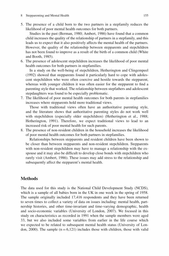
8 Stepparenting and Mental Health 155
5. The presence of a child born to the two partners in a stepfamily reduces thelikelihood of poor mental health outcomes for both partners.
Studies in the past (Berman, 1980; Ambert, 1986) have found that a commonchild increases the quality of the relationship of partners in a stepfamily, and thisleads us to expect that it also positively affects the mental health of the partners.However, the quality of the relationship between stepparents and stepchildrenhas not been found to improve as a result of the birth of a common child (Whiteand Booth, 1985).
6. The presence of adolescent stepchildren increases the likelihood of poor mentalhealth outcomes for both partners in stepfamilies.
In a study on the well-being of stepchildren, Hetherington and Clingempeel(1992) showed that stepparents found it particularly hard to cope with adoles-cent stepchildren who were often coercive and hostile towards the stepparent,whereas with younger children it was often easier for the stepparent to find aparenting style that worked. The relationship between stepfathers and adolescentstepdaughters was found to be especially problematic.
7. The likelihood of poor mental health outcomes for both parents in stepfamiliesincreases where stepparents hold more traditional views.
Those with traditional views often have an authoritative parenting style,and the literature shows that authoritative parenting styles do not work wellwith stepchildren (especially older stepchildren) (Hetherington et al., 1988;Hetherington, 1991). Therefore, we expect traditional views to lead to anincreased risk of poor mental health for such parents.
8. The presence of non-resident children in the household increases the likelihoodof poor mental health outcomes for both partners in stepfamilies.
Relationships between stepparents and resident children have been shown tobe closer than between stepparents and non-resident stepchildren. Stepparentswith non-resident stepchildren may have to manage a relationship with the ex-spouse and it may also be difficult to develop close bonds with stepchildren whorarely visit (Ambert, 1986). These issues may add stress to the relationship andsubsequently affect the stepparent’s mental health.
Methods
The data used for this study is the National Child Development Study (NCDS),which is a sample of all babies born in the UK in one week in the spring of 1958.The sample originally included 17,416 respondents and they have been returnedto seven times to collect a variety of data on issues including: mental health, part-nership histories, and other time-invariant and time-varying demographic, healthand socio-economic variables (University of London, 2007). We focused in thisstudy on characteristics as recorded in 1991 when the sample members were aged33, but we also included some variables from earlier in the life course whichwe expected to be related to subsequent mental health status (University of Lon-don, 2000). The sample (n = 6,121) includes those with children, those with valid

156 P. Feijten et al.
measures of behavioural/mental problems at age 16 and age 33, and those withfamily status information. Descriptive statistics for all the variables are given inTable 8.1.
Our outcome variable of interest is mental health. The measurement instrumentused to measure mental health in the NCDS is the Malaise Inventory Scale (MIS)developed by Rutter et al. (1970). It consists of 24 questions which are designedto capture depression and anxieties, obsessions and phobias. It has commonly been
Table 8.1 Descriptive statistics for variables used in the study
Variable Number Percentage
Mental health age 33Good health 5395 88.1Poor health 726 11.9
Behavioural problems at age 16Home Behaviour Scale score < 7 4823 78.8Home Behaviour Scale score >= 7 1298 21.2
Family type age 33First family 4638 75.8Lone parent 420 6.9Stepparent 400 6.5Partner of stepparent 494 8.1Both stepparents 169 2.8
SexMale 2,714 44.3Female 3,407 55.7
Employment statusFull-time working 3,264 53.3Part-time working 1,356 22.2Unemployed 195 3.2Other not working 1,306 21.3
Highest completed educational levelNo education completed 1,076 17.6CSE 2-5 1,201 19.6O levels 2,482 40.5A levels 604 9.9Degree 684 11.2Unknown 74 1.2
Social classUnskilled 280 4.6Partly skilled 1,046 17.1Skilled manual 1,137 18.6Skilled non-manual 1,388 22.7Managerial / technical 1,642 26.8Professional 212 3.5Unknown 416 6.8
Domestic tension age 7No 5,194 84.9Yes 255 4.2Unknown 672 11.0
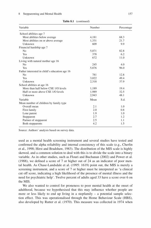
8 Stepparenting and Mental Health 157
Table 8.1 (continued)
Variable Number Percentage
School abilities age 7Most abilities below average 4,181 68.3Most abilities on or above average 1,331 21.7Unknown 609 9.9
Financial hardship age 7No 5,071 82.8Yes 378 6.2Unknown 672 11.0
Living with natural mother age 16No 245 4.0Yes 5,876 96.0
Father interested in child’s education age 16No 781 12.8Yes 3,022 49.4Unknown 2,318 37.9
School abilities at age 16More than half below CSE 1/O levels 1,189 19.4Half or more above CSE 1/O levels 1,989 32.5Unknown 2,943 48.1
Variable Mean S.d.Mean number of children by family type
Overall mean 2.1 1.0First family 2.0 0.8Lone parent 1.9 1.0Stepparent 2.7 1.2Partner of stepparent 2.5 1.1Both stepparents 4.2 1.5
Source: Authors’ analysis based on survey data.
used as a mental health screening instrument and several studies have tested andconfirmed the alpha reliability and internal consistency of this scale (e.g., Cherlinet al., 1998; Hirst and Bradshaw, 1983). The distribution of the MIS scale is highlyskewed, and a common solution to deal with this is to divide the scale into a binaryvariable. As in other studies, such as Flouri and Buchanan (2002) and Power et al.(1988), we defined a score of 7 or higher out of 24 as an indicator of poor men-tal health. As Chase-Landsdale et al. (1995: 1619) point out, the MIS is merely ascreening instrument, and a score of 7 or higher must be interpreted as ‘a clinicalcut off score, indicating a high likelihood of the presence of mental illness and theneed for psychiatric help’. Twelve percent of adults aged 33 have a score over 6 onthe MIS.
We also wanted to control for proneness to poor mental health at the onset ofadulthood, because we hypothesised that this may influence whether people aremore or less likely to end up living in a stepfamily – a potential sample selec-tion effect. This was operationalised through the Home Behaviour Scale (HBS),also developed by Rutter et al. (1970). This measure was collected in 1974 when

158 P. Feijten et al.
respondents were aged 16. The instrument consists of a 22-item scale that is meantto signal both externalizing (where the child shows under-controlled behavioursuch as aggression or disobedience) and internalizing (where the child showsover-controlled behaviour such as anxiety or depression) behavioural disorders inchildren. Again, a score of 7 or higher was chosen as a threshold for definingbehavioural problems. Twenty one per cent of children at age 16 have a score over6 on the HBS.
In order to distinguish different types of (step)families, we created a categoricalvariable with five categories: (1) respondents in first families, (2) respondents inlone parent families, (3) respondents who are stepparents, (4) respondents who arethe partners of stepparents and (5) respondents who are stepparents and partnersof stepparents at the same time (i.e., both partners have children from a previousrelationship). We label this group ‘dual stepfamilies’, and the results show that thisgroup is particularly important (not all studies consider this rarer group).
Finally, we extracted additional explanatory variables expected to influence men-tal health. We used variables from different points in the life course. Some reflectthe status of the sample respondents in the year of analysis, 1991, when respondentswere 33 years old. These included the sex of the respondent, their economic status,highest educational qualification and social class. We also included the number ofchildren in the family, as stepfamilies are larger than first families on average. Then,we included variables about respondents’ characteristics at ages 7 and 16, to controlfor previous circumstances expected to be associated with mental health outcomesin later life (see Cherlin et al., 1998; Flouri and Buchanan, 2002). These includeddomestic tension at age 7, financial hardship in the child’s household at age 7,whether the child lived with his/her natural mother at age 16, whether the father wasinterested in the child’s education at age 16, and school abilities at ages 7 and 16.
The method used is logistic regression, with mental health status at age 33(1991) as the binary dependent variable (0 = non-poor mental health; 1 = poor men-tal health). All models include the control variables described above, and the resultsare expressed as parameter estimates in the tables. We first estimated a model with-out behavioural problems in adolescence, and then a model that included this vari-able, where we were particularly interested in the effects of the interaction betweenbehavioural problems at age 16 and family status at age 33 on mental health sta-tus at age 33. We also graphed the coefficients by family status. In order to betterfacilitate appropriate visual comparisons between categories of the explanatory vari-able, we have plotted comparison intervals as suggested by Firth (2003) and furtherillustrated by Gayle and Lambert (2007).
Results
Description of Stepfamilies
We distinguish between stepparents, partners of stepparents, and familieswhere both partners are stepparents to each other’s children in our study

8 Stepparenting and Mental Health 159
Table 8.2 Demographic characteristics by family type
Average Average Average agenumber of number of range
Distribution children children (incl. childrenfamily type (resident non-resident (resident Average age(%) children only) children) children only) (step)parent∗
First family 75.6 2.0 2.0 2.8 33.3Lone parent family 7.2 1.7 1.9 3.0 –All stepfamilies 17.3 1.8 2.8 4.5 34.7
Stepparent 6.4 1.7 2.7 4.1 37.5Partner of stepparent 8.1 1.8 2.5 4.9 32.0Both stepparents 2.8 2.3 4.2 4.6 36.1
Source: Authors’ analysis based on NCDS sweep 1991.∗ This statistic is based on partners of NCDS cohort members, because cohort members themselveswere all aged 33 at the time of the survey.
(‘dual stepfamilies’). The distribution of respondents over these family types isshown in Table 8.2 (column 1). Table 8.2 also shows that adults living in stepfami-lies are different from adults living in first families and lone parent families, in termsof age, number of children in the household and the age range of these children (seealso Haskey, 1994). The second and third columns show the average number of chil-dren per family type (excluding and including non-resident children). Columns fourand five show the average age range of the children in the household, and the aver-age age of (step)parents per family type. It can be seen that adults in stepfamilies areon average older and have more children, who are of a wider age range, than peoplein first families and lone parent families.
Association Between Being a (Partner of a) Stepparentand Mental Health
Table 8.3 shows the numbers and percentages of people with poor and non-poormental health, by family type, at age 33. Adults in stepfamilies (both stepparentsand their partners) were more likely to suffer poor mental health than adults in firstfamilies, but less likely than lone parents.
Table 8.3 Poor mental health by family type
Non-poor mental health Poor mental health
n % N %
First family 5,631 90.7 575 9.3Lone parent family 434 73.9 153 26.1Stepfamily 176 83.1 240 16.9
Source: Authors’ analysis based on NCDS sweep 1991.

160 P. Feijten et al.
Health Selection into Stepfamilies?
As argued above, it is possible that part of this association is due to health selectioninto stepfamilies. Table 8.4 shows the numbers and percentages of people with andwithout behavioural problems at age 16 who ended up in a stepfamily at age 33.Those with behavioural problems at age 16 were significantly more likely to livein a stepfamily as an adult (22.9%) than those who had no behavioural problems atage 16 (15.9%). This supports the idea that at least part of the worse mental healthof (partners of) stepparents is due to the selection of people prone to poorer mentalhealth into stepfamilies. This is therefore accounted for in the models below.
Table 8.4 Behavioural problems at age 16 by stepfamily status at age 33
In a stepfamily at age 33?
Behavioural problemsNo Yes Total
at age 16? n % n % %
No 4,057 84.1 766 15.9 100Yes 1,001 77.1 297 22.9 100
Pearson chi2(1) = 34.9; p < 0.000.Source: Authors’ analysis based on NCDS sweeps 1974 and 1991.
Modelling Results
All hypotheses were tested in models with and without control variables, whichincluded: sex, household size, employment status, highest completed education,social class, domestic tension at age 7, financial hardship at age 7, school abilitiesat ages 7 and 16, living with the natural mother at age 16, and father interestedin education at age 16. Table 8.5 shows the results from two multivariate anal-yses. Model 1 does not take behavioural problems at age 16 into account whileModel 2 does.
We see, first of all, that the number of children in the household does not affectthe risk of having poor mental health (Model 1). Gender does have an influence:our result replicates the well-known finding that women have a higher risk of poormental health than men (Bird and Fremont 1991). The employment status variableshows that people who do not work are at increased risk of having poor mentalhealth, especially those who are unemployed. Also, those with lower levels of edu-cation and from lower social classes have an increased risk of poor mental health.
Childhood circumstances at age 7 also affect mental health at age 33. Livingin a household with domestic tension or financial hardship, or performing belowaverage at school increases the risk of being in poor mental health. Those who livedwith their natural mother or had a father who was interested in their education at age16 have better mental health at age 33. Also school abilities at age 16 are positivelyassociated with mental health at age 33. Our main variable of interest at age 16 iswhether the respondent had behavioural problems. Model 2 shows that those with

8 Stepparenting and Mental Health 161
Table 8.5 Modelling results for mental health status at age 33 (1991) (n = 6,121)
Model 1 Model 2
Variable Coef. p-value Coef. p-value
Constant –2.378 0.000 –2.470 0.000Behavioural problems age 16
HBS score < 7 0.000HBS score >= 7 0.554 0.000
Family type age 33First family 0.000 0.000Lone parent family 0.692 0.000 0.572 0.001Stepparent 0.401 0.017 0.282 0.187Partner of stepparent 0.329 0.017 0.211 0.240Dual stepfamily 0.869 0.000 0.966 0.000
Behavioural problems age 16 ∗ Family type age 33First family 0.000Lone parent family 0.194 0.468Stepparent 0.257 0.452Partner of stepparent 0.206 0.463Dual stepfamily –0.320 0.429
Number of children in the household (incl. non-resident ) –0.011 0.797 –0.021 0.630Sex
Male 0.000 0.000Female 0.658 0.000 0.624 0.000
Employment status age 33Fulltime working 0.000 0.000Part-time working –0.080 0.556 –0.076 0.576Unemployed 0.628 0.001 0.572 0.003Other not working 0.228 0.079 0.224 0.086
Highest completed educational level age 33No education completed 0.000 0.000CSE levels 2–5 –0.410 0.001 –0.373 0.002O levels –0.523 0.000 –0.481 0.000A levels –0.734 0.000 –0.663 0.001Degree or subdegree –1.064 0.000 –0.985 0.000Unknown –0.617 0.119 –0.528 0.184
Social class age 33Unskilled 0.000 0.000Partly skilled –0.157 0.371 –0.139 0.434Skilled manual –0.235 0.212 –0.219 0.250Skilled non-manual –0.431 0.018 –0.401 0.029Managerial / technical –0.510 0.008 –0.469 0.016Professional –0.802 0.063 –0.725 0.094Unknown 0.195 0.202 0.221 0.278
Domestic tension age 7No 0.000 0.000Yes 0.497 0.004 0.428 0.015Unknown –1.449 0.152 –1.454 0.158
Financial hardship age 7No 0.000 0.000

162 P. Feijten et al.Table 8.5 (continued)
Model 1 Model 2
Variable Coef. p-value Coef. p-value
Yes 0.370 0.012 0.360 0.016Unknown 1.474 0.141 1.471 0.149
School abilities age 7Most abilities on or above average 0.000 0.000Most abilities below average 0.231 0.023 0.215 0.037Unknown 0.070 0.736 0.080 0.702
Living with natural mother age 16No 0.000 0.000Yes –0.440 0.013 –0.433 0.015
Father interested in child′s education age 16No 0.000 0.000Yes –0.326 0.008 –0.332 0.008Unknown –0.279 0.018 –0.270 0.023
School abilities at age 16Half or more of subjects above CSE 1/O levels 0.000 0.000More than half of subjects below CSE 1/O levels 0.375 0.023 0.339 0.041Unknown 0.425 0.007 0.389 0.014
Source: Authors’ analysis based on survey data.
behavioural problems at age 16 had a significantly higher risk of poor mental healthat age 33. To summarise, most control variables, both at age 33 and in childhood,are associated with mental health in the hypothesised directions.
Family Type
Of particular interest were the effects of family type. Figure 8.1 graphs the regres-sion coefficients for the five family types (as in Model 1, Table 8.5). Compared tothose in first families, the risk of poor mental health is significantly higher for loneparents and all three types of stepfamily. For lone parents, the odds of poor mentalhealth are twice as high (exp (0.692) = 2.0) as for those in first families, and fordual stepfamilies 2.4 times as high (exp (0.869) = 2.38). The difference betweenpeople in first families and people in families with only one stepparent is smaller,yet significant at the 95% confidence interval level. These initial results are consis-tent with the hypothesis that the various strains involved in stepparenting may resultin poorer mental health for both stepparents and their partners compared to those infirst families, and that these strains are even stronger in more complex stepfamilieswhere both partners have stepchildren.
However, as we argued earlier, it is also possible that those prone to poorer men-tal health may be selected into stepfamilies, and we showed in section “ResearchQuestions and Data” that those with a high HBS score at age 16 were more likelyto end up in a stepfamily at age 33 than those with a low HBS score at age 16.Therefore, we controlled for behavioural problems in adolescence in Model 2, by

8 Stepparenting and Mental Health 163
1.4
1.2
1
0.8
0.6
0.4
0.2
0
–0.2
Est
imat
ed lo
gis
tic
effe
ct(r
egre
ssio
n c
oef
fici
ent)
Firstfamily
Dualstepfamily
Partnerof
stepparent
StepparentLoneparent
95% comparison interval
Fig. 8.1 Poor mental health at age 33 (1991) by family status (derived from Model 1,Table 8.5; Source: Authors’ analysis based on survey data.)
including an interaction between family type at age 33 and behavioural problemstatus at age 16.
Figure 8.2 shows the coefficients calculated from the main effects and inter-action effects of family type (at age 33) and behavioural problem status (at age16) from Model 2 (Table 8.4). Of those who had few behavioural problems at age
2
1.5
1
0.5
0
–0.5
Est
imat
ed lo
gis
tic
effe
ct(r
egre
ssio
n c
oef
fici
ent)
Firstfamily
Dualstepfamily
Partnerof
stepparent
StepparentLoneparent
HBS<7 HBS>=7 95% comparison interval
Fig. 8.2 Poor mental health at age 33 (1991) by family status (derived from Model 2,Table 8.4; Source: Authors’ analysis based on survey data.)

164 P. Feijten et al.
16 (HBS< 7), only lone parents and those couples where both partners were step-parents had significantly worse health than those in first families at age 33. Thisfits in with the finding from earlier studies that stepparent-stepchild relationshipswere more distant if both parents had their own children living in the household(Coleman and Ganong, 1990). In the more common stepfamilies, where only oneof the adults was a stepparent, neither the stepparents nor their partners had signifi-cantly worse health than those in first families, if they had few behavioural problemsat age 16.
On the other hand, the risk for those who had a high HBS score at age 16 wasconsiderably higher in every family status category. Comparing across the categoriesfor those with high HBS scores at age 16, we find that lone parents, stepparents andpartners of stepparents and partners who were both stepparents, all have a signif-icantly higher risk of poor mental health at age 33 than their counterparts in firstfamilies (although only significant at the 90% confidence interval level for partnersof stepparents and dual stepfamilies; note that the larger confidence interval for dualstepfamilies will partly be caused by the small number of observations in this cate-gory (n = 55)). Hence our results suggest that those who had behavioural problemsin adolescence are much more likely to suffer poor mental health in later life, butthat those who end up living in stepfamilies (and lone parent families) suffer a sig-nificantly heavier burden on their mental health.
Finally, we compare those with and without behavioural problems at age 16within each family type. For those in first families who had high HBS scores atage 16 the risk of having poor mental health at age 33 was significantly higher thanfor those in first families with low HBS scores at age 16. Also, lone parents, step-parents and partners of stepparents have a significantly higher risk of having poormental health if they had high HBS scores at age 16 than if they had low scores.For dual stepfamilies there is no difference in poor mental health risk for those withand without behavioural problems in adolescence. For both groups the risk is high,indicating that living in a stepfamily with children from both partners’ previous rela-tionships leads to stress and worries, no matter what the prior mental health status.
The next five hypotheses, concerning the characteristics of the adults and thechildren in stepfamilies, were tested in multivariate models with the same set ofcontrol variables as shown in Table 8.4. The effects of the control variables in allmodels were very comparable to those in Table 8.4 and are not discussed further.
Characteristics of the Adults in Stepfamilies
We hypothesised that being poor affects the mental health of those in stepfami-lies, because financial problems are a primary source of stress. We measured socio-economic background in three ways: highest completed level of education, socialclass and economic activity status (income information in the NCDS is not suitablefor this present analysis as it includes a lot of missing data, so we did not use it).Each dimension shows the same picture, but the results for labour market activityare the most marked, and remain largely significant after controlling for background

8 Stepparenting and Mental Health 165
variables. The results show that people who do not work have a higher risk of poormental health than people who work. Among those who work, those working part-time have a slightly elevated risk of poor mental health compared to full-time work-ers, but only in the model without control variables. Overall, our findings confirmthat adults in stepfamilies with poorer socio-economic circumstances have a higherrisk of having poor mental health. However, we also find this effect for adults in firstfamilies and lone parent families, so it is not exclusively true for stepfamilies. Whenwe control for background variables, the effects of level of education and socialclass remain in the same direction, but their magnitude decreases and they becomelargely insignificant.
Our next hypothesis was that the younger the stepparent, the greater the nega-tive impact of stepparenting on mental health. In the NCDS, it is not possible totest hypotheses about age differentiation directly, because NCDS cohort membersare all the same age. However, we explored this by comparing results at age 33(NCDS sweep 1991) and age 41/42 (NCDS sweep 2000). Comparison of the resultsshows that differences in mental health between those in first families and those instepfamilies were larger at age 33 than at age 41/42, confirming our hypothesis. Ofparticular interest is the finding that at age 33, adults in stepfamilies have a higherrisk of poor mental health than those in first families, and this difference has disap-peared at age 41/42 (although, only for those with behavioural problems at age 16in the model with control variables). When we compare those who did and did nothave behavioural problems in adolescence within each family type, we also see thatdifferences were bigger at age 33 than at age 41/42.
Last, we find some confirmation for our hypothesised effect of traditional atti-tudes on the likelihood of poor mental health for adults in stepfamilies. We didthis analysis on the data at age 41/42, with attitudes as measured at age 33 (priorattitudes should provide a better explanation of current behaviour than current atti-tudes, as the direction of effect is difficult to determine if both are measured con-currently). A traditional attitude was measured as a cumulative score on severalattitudinal items such as “wives who don′t have to work should not do so”. Theresults show that adults in lone parent families and dual stepfamilies who held moretraditional views at age 33 have a slightly higher risk of poor mental health at age41/42 than their counterparts who held less traditional views (although, only signif-icant for those who had no behavioural problems in adolescence). For people in firstfamilies and ‘single’ stepfamilies, attitude does not affect mental health. For peoplewho had behavioural problems in adolescence, attitude has no effect for stepfami-lies and lone parent families, but it does for first families (the more traditional, thehigher the risk of poor mental health).
Characteristics of the Children in Stepfamilies
The presence of a child born to both parents in a stepfamily was expected to reducethe risk of poor mental health, because it can cement the bond between family mem-bers and provide more role clarity to the stepparent. We found marginal support for

166 P. Feijten et al.
this, as having common children did reduce rates of mental illness, but none of thedifferences between adults in stepfamilies with and without common children werestatistically significant, even in the models without control variables.
The presence of adolescent children (age 13–17) in the household does increasethe likelihood of poor mental health, but this is true for all family types, not juststepfamilies. In fact, the effect is greatest for adults in first families. When we con-trol for background variables, the differences between families with and withoutadolescent children disappears, except for those in first families and those in dualstepfamilies who had no behavioural problems in adolescence.
Lastly, we studied the effect of having non-resident children (that is, either orboth adults in the stepfamily have a child or children who live(s) somewhere else,usually with the other biological parent) on mental health. We expected that hav-ing non-resident children would increase the risk of mental health problems. Firstly,for the parent him/herself because (s)he is always in the shadow of the parent withwhom the children live, and because (s)he may miss the child(ren) and suffer fromfeelings of guilt that (s)he does not spend more time with them. The stepparents ofnon-resident children may also find it difficult to cope with stepchildren who theyonly see infrequently, and to support their partner. Our results show a consistenteffect of having non-resident children in both the models with and without controlvariables. Lone parents and adults in stepfamilies with non-resident children aremore likely to have mental health problems than their counterparts who do not havenon-resident children. The differences between those with and without non-residentchildren are particularly large among people who had behavioural problems inadolescence.
Summary and Conclusions
This study has shown that there are significant differences in mental health betweenadults in first families and different types of stepfamilies. Stepparents themselves,and their partners, are more at risk of having poor mental health than their coun-terparts in first families. When both adults in a stepfamily are stepparents to eachother’s children, their mental health is even more at risk.
However, as we also showed, part of this association is due to the fact that adultswho live in stepfamilies are more prone to poor mental health in the first place.This ‘proneness to poor mental health’ was captured using a variable that measuredbehavioural problems at age 16, which is a good predictor of mental health problemsin later life. Those who had behavioural problems at age 16 were more likely to endup in stepfamilies, and therefore make up a larger proportion of the stepfamily pop-ulation than they do of the first family population. The temporal ordering of theseevents means that cross-sectional data would not allow this issue to be explored.Evenson and Simon (2005), for example, show a higher likelihood of depressionamong some types of stepparents compared to parents in first families, but theyacknowledge in their discussion that this may partly be due to selection into andout of stepfamilies of people with different prior mental health status (interestingly,

8 Stepparenting and Mental Health 167
they speculate that it may be people with better initial mental health who selectthemselves into stepfamilies).
Once we took prior mental health into account, we found that stepfamily life isparticularly harmful to the mental health of people who had behavioural problems inadolescence. They appear to find it hard to cope with the role of being a stepparent,or the partner of a stepparent, possibly because of the problems and tensions in step-families that are largely absent in first families. Adults who did not have behaviouralproblems as an adolescent only have an increased risk of poor mental health if theylive in dual stepfamilies or lone parent families.
Several other elements of stepfamilies were also shown to account for the adverseeffect of stepfamily life on mental health. When stepfamilies have non-resident chil-dren, that is, one (or both) of the adults has children who live in another house-hold, this increases the risk of poor mental health. The age of the stepparent alsomattered: the younger they were, the higher the likelihood of poor mental health.Other factors increasing the likelihood of poor mental health in stepfamilies are: notworking, or working part-time (compared to working full-time), and having adoles-cent (step)children in the household. However, these factors also increase the risk ofpoor mental health for adults in the other family types (first families and lone parentfamilies), and are thus not only true for stepfamilies.
This study is one of the first of its type to compare the risk of mental health prob-lems for stepparents, or partners of stepparents, compared to those in first families.Although we could not directly compare our outcomes with any previous studies,the results do conform to studies on related topics. Studies arguing that stepfamiliesare more stressful environments than first families (such as Brown and Booth, 1996;Pryor and Rodgers, 2001) seem to be supported by our findings. Also, the worsemental health of people in stepfamilies may affect marital quality and marital stabil-ity of couples in stepfamilies. This would provide an additional explanation for themarkedly higher divorce rates found in remarriages that involve stepchildren. Suchmarriages have been found to suffer from worse marital quality (e.g. Coleman andGanong, 1990; Pasley et al., 1993), but the explicit link with mental health has notbeen made in such studies.
It is also possible that our results underestimate the adverse effect of stepfam-ily life on mental health. If those who find it hard to cope with being a (partnerof a) stepparent are more likely to end the relationship, they will be ignored inour analysis. While their mental health may have been most seriously affected bystep-parenthood, leaving the relationship may have caused improvements making itdifficult to estimate the effect of stepparenting. Only long-running panel data (withfrequent waves) would allow us to examine such a case, as we would be able toobserve people entering and exiting different types of households over their lifecourse, and relate their (changing) family type to their mental health status.
Our results demonstrate the value of longitudinal analysis, which has allowed thesubtlety of the relationship between stepparenting and mental health to be exploredand we support Coleman et al.’s (2000) plea for more longitudinal analyses of com-plex family circumstances. Clearly, the health outcomes for stepparents and theirpartners would appear to deserve more attention and the results of such analyses

168 P. Feijten et al.
may be of interest to family researchers, as well as clinicians and counsellors work-ing with adults who are struggling with stepparenting issues.
References
Allan, G. (1999) The Sociology of the Family, Oxford, Blackwell.Amato, P.R. (2000) The consequences of divorce for adults and children, Journal of Marriage and
the Family, 62: 1269–1287.Ambert, A.M. (1986) Being a stepparent: Live-in and visiting stepchildren, Journal of Marriage
and the Family, 48: 795–804.Avlund, K., Damsgaard, M.T. and Holstein, B.E. (1998) Social relations and mortality. An eleven
year follow-up study of 70-year-old men and women in Denmark, Social Science and Medicine,47: 635–643.
Berkman, L.F. and Syme, S.L. (1979) Social networks, host resistance, and mortality: A nine-year follow-up study of Alameda County residents, American Journal of Epidemiology, 109:186–204.
Berman, C. (1980) Making it as a Stepparent: New Roles/New Rules. Garden City (NY),Doubleday.
Bird, C.E. and Fremont, A.M. (1991) Gender, time use, and health, Journal of Health and SocialBehavior, 32: 114–129.
Brown, S.L. and Booth, A. (1996) Cohabitation versus marriage: A comparison of relationshipquality, Journal of Marriage and the Family, 58: 668–678.
Chase-Landsdale, P.L., Cherlin, A.J. and Kiernan, K.E. (1995) The long-term effects of parentaldivorce on the mental health of young adults: A developmental perspective, Child Development,66: 1614–1634.
Cherlin. A.J. (1978) Remarriage as an incomplete institution, American Journal of Sociology, 86:634–650.
Cherlin, A.J., Chase-Lansdale, P.L. and McRae, C. (1998) Effects of parental divorce on mentalhealth throughout the life course, American Sociological Review, 63(2): 239–249.
Clingempeel, G. (1981) Quasi-kin relationships and marital quality, Journal of Personality andSocial Psychology, 41: 890–901.
Coleman, M. and Ganong, L.H. (1990) Remarriage and stepfamily research in the 1980s: Increasedinterest in an old family form, Journal of Marriage and the Family, 52: 925–940.
Coleman, M., Ganong, L. and Fine, M. (2000) Reinvestigating remarriage: Another decade ofprogress, Journal of Marriage and the Family, 62: 1288–1307.
Del Carmen, M., Alcon, G., Pedersen, J.M., Maria, A. and Gonzalez, C. (2002) Greenlandic familystructure and communication with parents: Influence on schoolchildren’s drinking behaviour,International Journal of Circumpolar Health, 61: 319–331.
Duncan, G.J. and Hoffman, S.D. (1985) A reconsideration of the economic consequences of maritaldissolution, Demography, 22: 485–497.
Ermisch, J. and Francesconi, M. (2000) The increasing complexity of family relationships: Life-time experience of lone motherhood and stepfamilies in Great Britain, European Journal ofPopulation, 16: 235–249.
Evenson, R.J. and Simon, R.W. (2005) Clarifying the relationship between parenthood and depres-sion, Journal of Health and Social Behaviour, 46: 341–358.
Fergusson, D.M., Lynskey, M.T. and Horwood, L.J. (1994) The effects of parental separation, thetiming of separation and gender on children’s performance on cognitive tests, Journal of ChildPsychology and Psychiatry and Allied Disciplines, 35: 1077–1092.
Ferri, E. and Smith, K. (1998) Stepparenting in the 1990s, Family Policy Studies Centre, London.Finch, N. (2002) Demographic Trends in the UK, Social Policy Research Unit, University of York,
York.Firth, D. (2003) Overcoming the reference category problem in the presentation of statistical mod-
els, Sociological Methodology, 33(1): 1–18.

8 Stepparenting and Mental Health 169
Flouri, E. and Buchanan, A. (2002) The role of father involvement in children’s later mental health,Journal of Adolescence, 26: 63–78.
Gardner, J. and Oswald, A. (2004) How is mortality affected by money, marriage, and stress?Journal of Health Economics, 23: 1181–1207.
Gayle, V. and Lambert, P. (2007) Using quasi-variance to communicate sociological results fromstatistical models, Sociology, 41: 1191–1207.
Haskey, J. (1994) Stepfamilies and stepchildren in Great Britain, Population Trends, 76: 17–28.Hetherington, E.M., Arnett, J.D. and Hollier, E.A. (1988) Adjustment of parents and children in
remarriage, in Wolchick, S.A. and Karoly, P. (eds.) Children of Divorce, University of ChicagoPress, Chicago, pp. 67–107.
Hetherington, E.M. (1991) Presidential address: Families, lies and videotape, Journal of Researchon Adolescence, 1: 323–348.
Hetherington, E.M. and Clingempeel, W.G. (1992) Coping with marital transitions: A family sys-tems perspective, Monographs of the Society for Research in Child Development, 57: 2–3 (serialno. 227).
Hetherington, E.M. and Jodl, K.M. (1994) Stepfamilies as settings for child development, in Booth,A. and Dunn, J. (eds.) Stepfamilies: Who Benefits? Who Does Not?, Lawrence Erlbaum Asso-ciates, Hillsdale (New Jersey), pp. 55–80.
Hirst, M.A. and Bradshaw, J.R. (1983) Evaluating the malaise inventory: A comparison of mea-sures of stress, Journal of Psychosomatic Research, 27(3): 193–199.
Hope, S., Power, C. and Rodgers, B. (1999) Does financial hardship account for elevated psycho-logical distress in lone mothers?, Social Science and Medicine, 49: 1637–1649.
Joshi, H., Cooksey, E., Wiggins, R., McCulloch, A., Verropoulou, G. and Clarke, L. (1999) Diversefamily living situations and child development: A multi-level analysis comparing longitudinalevidence from Britain and the United States, International Journal of Law, Policy and the Fam-ily, 13: 292–314.
Keirnan, K. and Mueller, G. (1998) Who are the divorced, and who divorces? CASEbrief 6, Centrefor Analysis of Social Exclusion, London.
Mekos, D., Hetherington, E.M. and Reiss, D. (1996) Sibling differences in problem behaviour andparental treatment non-divorced and remarried families, Child Development, 67: 2148–2165.
Neff, J.A. and Schluter, T.D. (1993) Marital status and depressive symptoms: The role ofrace/ethnicity and sex, Journal of Divorce and Remarriage, 20: 137–160.
Pagani, L., Tremblay, R.E., Vitaro, F., Kerr, M. and McDuff, P. (1998) The impact of family transi-tion on the development of delinquency in adolescent boys: A 9-year longitudinal study, Jour-nal of Child Psychology and Psychiatry and Allied Disciplines, 39: 489–499.
Palisi, B.J., Orleans, M., Caddell, D. and Korn, B. (1991) Adjustment to stepfatherhood: The effectsof marital history and relations with children, Journal of Divorce and Remarriage, 14(3/4):89–106.
Pasley, K., Dollahite, D.C. and Ihinger-Tallman, M. (1993) Clinical applications of research find-ings on the spouse and stepparent roles in remarriage, Family Relations, 42: 315–322.
Pong, S.L. (1997) Family structure, school context, and eighth grade math and reading achieve-ment, Journal of Marriage and the Family, 59: 734–746.
Power, C., Manor, O., Fox, J. and Fogelman, K. (1988) Health selection: An explanation ofsocial inequalities in health in young adults? NCDS Working Paper 28, City University,London.
Pryor, J. and Rodgers, B. (2001) Children in Changing Families: Life After Parental Separation,Blackwell, London.
Ram, B.L. and Hou, F. (2003) Changes in family structure and child outcomes: Roles of economicand familial resources, Policy Studies Journal, 31: 309–330.
Richards, M., Hardy, R., and Wadsworth, M. (1997) The effects of divorce and separation onmental health in a national UK birth cohort, Psychological Medicine, 27: 1121–1128.
Rutter, M., Tizard, J. and Whitmore, K. (1970) Education, Health and Behaviour, Longman,London.

170 P. Feijten et al.
Seeman, T.E., Kaplan, G.A., Knudsen, L., Cohen, R. and Guralnik, J. (1987) Social network tiesand mortality among the elderly in the Alameda County Study, American Journal of Epidemi-ology, 126: 714–723.
Shouls, S., Whitehead, M., Burstrom, B. and Diderichsen, F. (1999) The health and socio-economiccircumstances of British lone mothers over the last two decades, Population Trends, 95: 41–46.
Simpson, B. (1994). Bringing the ‘unclear’ family into focus: Divorce and re-marriage in contem-porary Britain, Man, New Series, 29: 831–851.
Smart, C. (2003) Introduction: New perspectives on childhood and divorce, Childhood, 10:123–129.
Teachman, J.D., Paasch, K. and Carver, K. (1996) Social capital and dropping out of school early,Journal of Marriage and the Family, 58: 773–783.
Trovato, F. and Lauris, G. (1989) Marital status and mortality in Canada: 1951–1981, Journal ofMarriage and the Family, 51: 907–922.
University of London (2000). Institute of Education. Centre for Longitudinal Studies, NationalChild Development Study: Sweeps 1 (1965), 2 (1969) and 3 (1974) [computer file]. NationalBirthday Trust Fund, National Children′s Bureau and City University Social Statistics ResearchUnit [original data producer(s)]. UK Data Archive, University of Essex, Colchester [distribu-tor], 25 July 2000 (2nd Edition). SN: 3148.
University of London (2007). Institute of Education. Centre for Longitudinal Studies, NationalChild Development Study: Sweep 5, 1991 [computer file]. City University. Social StatisticsResearch Unit, [original data producer(s)]. Colchester, Essex: UK Data Archive [distributor],January 2007. SN: 5567.
Utting, D. (1995) Family and Parenthood: Supporting Families, Preventing Breakdown, JosephRowntree Foundation, York.
Wade, T.J. and Pevalin, D.J. (2004) Marital transitions and mental health, Journal of Health andSocial Behavior, 45: 155–170.
Wadsworth, J., Burnell, I., Taylor, B. and Butler, N. (1985) The influence of family type on chil-dren’s behaviour and development at five years, Journal of Child Psychology and Psychiatry,26: 245–254.
Walper, S. (1995) Family relationships and adolescents social development in nuclear, singlemother, and stepfather families, Zeitschrift fur Entwicklungspsychologie und PadagogischePsychologie, 27: 93–121.
White, L.K. and Booth, A. (1985) The quality and stability of remarriages: The role of stepchildren,American Sociological Review, 50: 689–698.
Zill, N. (1988) Behavior, achievement, and health problems among children in stepfamilies: Find-ings from a national survey of children health, in Hetherington, E.M. and Arasteh, J. (eds.)The Impact of Divorce, Single Parenting and Stepparenting on Children, Lawrence ErlbaumAssociates, Hillsdale, New Jersey, pp. 325–368.

Chapter 9Grandparents and the Careof Their Grandchildren
Alison Smith Koslowski
Introduction
Across Europe, certain grandparents are being relied upon to provide informal carefor their grandchildren, particularly as part of a package of early-years childcareprovision (Gray, 2005; Lewis et al., 2008). The increased participation of womenin the labour market (Crouch, 1999), without concomitant and equivalent increasedparticipation of men in informal care (Hook, 2006) means that the demand for infor-mal care is likely to increase whilst supply decreases. Evidence suggests that grand-parents are the informal carers of choice after the parents themselves (Wheelockand Jones, 2002). However, certain interest groups representing grandparents haveraised the concern that grandparents may be making a rather larger contribution tothe care and upbringing of their grandchildren than they had anticipated (e.g. AgeConcern, 2006). Regular primary care of small children is a time consuming activity,which is both physically and emotionally demanding and as such, not a task thatgrandparents had necessarily envisaged as a core part of their grandparental role.
There has been an increasing focus on informal care provision by mothers andtheir subsequent labour market and other outcomes (e.g., Joshi et al., 1999) and less,but some work, on informal care provision by fathers (Smith Koslowski, 2008).There has also been recognition of the prevalence of the informal care providedby older people for other older people, whether care for a spouse or for veryelderly parents (e.g., Bolin et al., 2007). However, there has been little researchin Europe into informal care provision by grandparents for grandchildren. Esti-mates for the value of unpaid childcare provided by grandparents in the UK suggestconsiderable activity, ranging from £3,886 million a year (Age Concern, 2004),to £50 billion (Rowlatt, 2007) to £220 billion (Greengoss, 2007). Such macro-economic accounting relies in part on information about the time use of olderpersons.
A.S. Koslowski (B)School of Social and Political Science, University of Edinburgh, Edinburgh, UKe-mail: [email protected]
J. Stillwell et al. (eds.), Fertility, Living Arrangements, Care and Mobility, UnderstandingPopulation Trends and Processes 1, DOI 10.1007/978-1-4020-9682-2 9,C© Springer Science+Business Media B.V. 2009
171

172 A.S. Koslowski
For grandparents, there may well be financial implications associated with car-ing informally for their grandchildren, although the costs and benefits will certainlyextend beyond the financial, including implications for health, volunteer work andleisure (for example, Bamford et al., 1998). For grandchildren, distinct develop-mental outcomes for children are associated with being cared for by a grandparent(e.g., Hansen and Hawkes, 2009). In order to calculate and thus understand thecosts and benefits of grandparental informal childcare, the first step is to obtaindata, which tell us about the amount of time grandparents spend looking after theirgrandchildren.
If policy makers are concerned to increase the supply of informal care, the impor-tance of support, financial and otherwise for individual care providers, requires con-sideration. It may be that an increased reliance on grandparents as informal carers isin contradiction with other policy goals associated with ‘active ageing’, concernedwith raising the employment rates of older people (Lewis et al., 2008). However, abroader definition of ‘active ageing’ may incorporate and recognise such informalcare work. The provision of informal grandparental childcare is likely to be gen-dered. Whilst grandfathers as well as grandmothers are shown to be active childcarers, grand-maternal care is more prevalent (Gray, 2005). Such gendered informalcare is likely to be one of several contributory factors leading to women in later lifeexperiencing an increased risk of poverty than men (Price, 2006). A review of thetime spent looking after children by grandparents, is a first step in the process ofassessing the implications of grandparental childcare for the grandparents involved,be they financial and otherwise, positive or negative.
The role of grandparents and their contribution to society is increasing in pro-file, not least due to there being more grandparents than ever before as mortalitydecreases, despite a substantial decline in fertility (cf. Murphy and Grundy, 2003),and due to the increase in divorce rates and subsequent extended family, result-ing in more complex grandparent and step-grandparent relationships. Indeed, anarray of dynamic demographic factors including increasing life expectancy, delayedchildbearing, decreasing fertility rates, teenage pregnancy rates and increased inter-generational geographic mobility contribute to the complexity of this issue. Therehas been somewhat of a lull in the latter part of the twentieth century as regardsresearch into extended family relations (Dench and Ogg, 2002). As such, it is diffi-cult to contextualise grandparental time in recent historical perspective and to knowwhether there is a revival of extended family relations, or if ties are as active as theyever were.
This chapter presents a cross-national review of the time that grandparents reportspending on childcare in Western Europe. Estimates are largely drawn from datarepresenting the time period 1994–2005. First, the various forms of grandparentalchildcare are presented, introducing the focus of the chapter, namely whether thegrandparent is acting as an informal childcare provider typically whilst the parentsgo out to work, although grandparents might also provide informal care as respitefor non-working parents. Second, the extent to which informal grandparental child-care can be expected to vary across Western Europe is discussed. Inevitably, dif-ferent welfare state systems create varying circumstances with regard to childcare

9 Grandparents and the Care of Their Grandchildren 173
provision and parental household employment patterns. A discussion of the com-plexity of the measurement of grandparental childcare time then precedes a reviewof currently available estimates.
Grandparents as Informal Childcare Providers
The initial picture of grandparents spending time with their grandchildren per-haps conjures up thoughts of Sunday afternoon family visits and proudly displayedschool photographs and no doubt, this is a grandparental model for many families.A concern of this chapter however, is to highlight a particular category of grand-parental childcare; that where the grandparent is a primary informal carer on aregular basis. The use of the term ‘primary’ indicates the parents’ absence typ-ically for a period of hours at any one time, but in some cases more long termto the extent of surrogate parenting. Grandparental childcare that extends beyondmulti-generational family visits and holidays can be said to exist in two forms. Thefirst form is where the grandparent becomes a co-residential surrogate parent to thegrandchild. The second form is where the grandparent becomes the primary infor-mal childcare provider. The latter is the more commonplace. Both across and withinthese categories of grandparental childcare, grandparents are a heterogeneous group,not least in terms of health, wealth and age.
Co-residential childcare carried out by grandparents acting as surrogate parentsis the form of grandparental childcare that has attracted most research attentionin recent years, though much of this literature is non-European (Hirshorn, 1998;Richards, 2001; Grandparents plus and Adfam, 2006; Brennan and Cass, 2007;MacKenzie, 2007). This particular form of grandparental childcare occurs in theevent of parental failure, whether as the result of the death of the parents, or morecommonly, a parental custodial prison sentence or substance abuse. In such cases,grandparents will frequently step in and take on the role of surrogate parent. Socialworkers may refer to grandparental care as a subset of kinship care. The supportof grandparents has been identified as a significant protective factor for children(Kroll, 2007) as kinship placements are more likely to enable children to remainwithin a family network than placements with non-kin carers (Broad, 2004). How-ever, complications for the grandparents may be caused by uncertain legal status,prior relationship difficulties with the parents, and factors such as their health,wealth and age (as described in Kroll, 2007). This group of grandparents are perhapsparticularly vulnerable and in need of state support. The number of grandparents act-ing as surrogate parents is relatively small; Clarke and Cairns (2001) estimate that1% of grandparents in Britain had grandchildren living with them on such a basis.
A small number of grandparents are co-resident with their children and grand-children. The percentage of parental households with resident grandparents anddependent children ranges from just 0.12% in the Netherlands to 15.6% in Portugal(Table 9.1). Single grandparents living with children are more likely to look aftergrandchildren, compared to those who do not live with their children (Croda andGonzalez-Chapela, 2005).

174 A.S. Koslowski
Table 9.1 Co-resident parental households containing grandparents and dependent children
% householdswithgrandparents N
Portugal 15.64 25,566Greece 14.98 24,190Austriab 14.13 13,066Spain 11 31,584Luxembourga 6.85 1,984Italy 6.41 36,204Ireland 5.51 17,146UKa 2.22 6,852Germanya 1.89 7,288Belgium 1.5 14,036Finlandc 1.45 14,040France 1.29 29,234Denmark 0.47 10,952Netherlands 0.12 22,124
Source: ECHP pooled sample 1994–2001 inclusive as available,author’s calculations.a Data coverage 1994–1996 inclusive.b Data coverage 1995–2001 inclusive.c Data coverage 1996–2001 inclusive.
More commonplace, but less evident in the literature are those non-residentialgrandparents providing regular informal childcare in the absence of the parents.Informal childcare may be met with some cash payment, but frequently other formsof reciprocity and redistribution come into play, commonly fulfilled over a longperiod of time. In contrast, formal childcare can be defined as that provided byexternal private service providers, the state or by not-for-profit organisations (Land,2002). In the latter quarter of the last century and into the present decade, therehas been significant growth in the employment rates of mothers (Crouch, 1999).There is cross-national variation, but this is an overall European trend (Lewiset al., 2008). The Lisbon Agenda, as set out by the European Council in March2000, is an action and development plan for the European Union which, amongother priorities, promotes the active employment of women with dependent chil-dren, including lone mothers. Many of these women will have young children whorequire childcare, and grandparents are an important source, as recognised by theUK Government in its 1998 consultation paper Supporting Families. Indeed, muchevidence points to grandparents being the most important source of such care insome countries, including the UK (Douglas and Ferguson, 2003; Bradshaw et al.,2008).
There is as yet little to no financial assistance for grandparents who are caringfor their grandchildren as primary informal care providers (Douglas and Ferguson,2003; Rowlatt, 2007). Currently, such grandparent childcarers are rarely eligible forstatutory support. In Hungary, grandparents have the possibility to take over some

9 Grandparents and the Care of Their Grandchildren 175
of the paid parental leave afforded to parents (Szikra, 2008). Portugal offers theopportunity for the mother of an under-age teenage mother to take parental leave inher place (OECD, 2004).
Informal care is for many parents a positive choice (Land, 2002). Informal carearrangements may be better able to withstand the complex timetabling associatedwith atypical working hours (Le Bihan and Martin, 2004). This preference may beassociated with the affordability, availability and quality of formal childcare pro-vision, all characteristics which vary cross-nationally. Whilst many grandparentsprovide regular primary informal childcare willingly, there is some evidence to sug-gest that a significant minority would prefer not to take on such an intense role, butrather keep to a less involved grandparental status (Dench and Ogg, 2002; Douglasand Ferguson, 2003).
There is considerable heterogeneity within the members of the population whomight describe themselves as grandparents. It is difficult to generalise the life stageat which grandparents may find themselves, as grandparenting is a contingent andcomplex process (Kemp, 2003). Becoming a grandparent can occur at anytime fromaround 35 years to 75 years of age and beyond. Evidence suggests that 27% of allgrandparents across Western Europe are below the age of 60, and so not of retire-ment age (Hank and Buber, 2007). The high prevalence of teenage pregnancy inthe UK, has led to a relatively high prevalence of young grandparents, themselvesstill of child bearing age (BBC3, 2008). This group of grandparents are particularlylikely to be turned to for informal primary childcare (Anderson et al., 2007). Atthe other end of the socio-economic spectrum, delayed childbearing leads to a rel-atively high prevalence of older grandparents. The opportunity costs, in particularthe financial implications of becoming a grandparent at various stages along the lifecourse will differ according to whether a person is still active in the labour market,non-employed or retired.
Grandparental childcare is a gendered activity. Various studies show thatmaternal grandparents appear to be more significant in the life of grandchildrenthan paternal grandparents, and that grandmothers appear to be more involvedthan grandfathers (Dench and Ogg, 2002; Douglas and Ferguson 2003). Addingfurther complexity, many grandchildren will have more than four grandparentalfigures in their lives (e.g. Kemp, 2003; Bradshaw et al., 2008). Largely this is theresult of parental divorce and re-partnering as well as grandparental divorce andre-partnering, both of which lead to step-grandparenthood. Social grandparentingrefers to those who take on a grandparenting role without necessarily being boundby biological ties. Depending on survey construction, studies often implicitly collectdata from social grandparents.
In brief, two forms of grandparental childcare have been outlined; surrogate par-enting and primary informal childcare provision. The focus of this chapter is on thelatter category, predominantly because the former group is not large enough to bepicked up by most survey data collection due to relatively small sample sizes. Whilstthis does represent a particular form of grandparental contact and childcare, thosegrandparents involved cannot be considered to be a homogenous group. The het-erogeneity between those grandparents giving regular informal care has potentially

176 A.S. Koslowski
important consequences for the financial implications and other associated costs orbenefits to the provider of such care work.
Determinants of Cross-National Variation in InformalGrandparental Childcare Provision
Cultural differences and nationally specific institutional structures will contributeto cross-national variation in grandparental care. Furthermore, by comparing acrosscountries we can explore whether socio-economic factors are consistently corre-lated with grandparental time spent on informal childcare provision. If this is foundto be the case, variation in prevalence of informal grandparental childcare provisionmay be explained in part by compositional differences. In this section, the implica-tions for grandparental care of variation in state intervention and parental householdemployment patterns are particularly explored.
Grandparental care is likely to become increasingly important when parents, par-ticularly mothers, are involved in employment. To the extent that children are apublic good, the state can ease the difficulties associated with combining parent-hood and work. How it does so will affect the prevalence of grandparental childcareas mediated by the demands on the parents. Government regulated childcare pro-visions can be classified into three distinct categories (Ditch et al., 1996): firstly,cash transfers (via fiscal policies, family allowances and other forms of social assis-tance); secondly, provision of services (e.g., the public provision of childcare), andthirdly, leave from the labour market. Generous cash transfers and provision of ser-vices in particular will enable parents to draw on formal care rather than rely oninformal care by grandparents. If parents are better supported financially and in theabsence of very high childcare costs, working long hours for more money may proveunnecessary. Statutory leave provisions are positively associated with the time thatmothers and fathers spend looking after their children (Smith and Williams, 2007).If parents are able to spend more time caring for their children, again the burden ongrandparents will be reduced.
Assuming the involvement that grandparents may continue to have, even in lightof the better case scenarios described above, the state can also introduce forms ofadditional social assistance for grandparental carers, and/or a form of (paid) leavefrom the labour market.
The European Union provides an ideal opportunity for comparative work. Whilstthe member states share a common institutional framework, there is also internaldiversity in terms of the welfare states, the governing institutions, traditions andcultures, which allows for variation in the explanatory variables. Additionally, thereis also a practical rationale for focusing on the EU-15: the data situation is optimalfor these countries.
There has been some considerable debate on whether there has been a Euro-pean welfare state convergence or divergence (see Castles, 2004), and there is aburgeoning literature on the more recent emergence of the European social model

9 Grandparents and the Care of Their Grandchildren 177
(e.g., Esping-Andersen et al., 2002). The basic premise of a European social modelis that the EU institutions harmonise social policy in Europe so as to provide socialprotection in a distinct fashion from that found elsewhere in the developed world(Castles, 2004).
The Social Chapter was adopted at the European Council in December 1989 byall member states except the UK (EC, 1990) and included the statement that “mea-sures should also be developed enabling men and women to reconcile their occupa-tional and family obligations” (CEC, 1989, p. 5, cited in Neilson, 1998, p. 72). InDecember 1991, at Maastricht, the member states (with the exception of the UK)agreed to implement the Social Chapter by means of the Protocol on Social Policyand the Agreement on Social Policy, which was annexed to the Treaty on EuropeanUnion (EC 1992; Neilson, 1998), thus writing mother- and father-friendly policyconcerns firmly into the agendas of the member states.
A council recommendation in 1992 (92/241/EEC) was passed, in which memberstates are encouraged to take and/or progressively encourage initiatives to enablewomen and men to reconcile their occupational, family and upbringing responsibil-ities arising from the care of children (Article 1). A recommendation such as this isan example of soft law, meaning that, unlike hard law, there are no sanctions on non-compliance. No mention was made of grandparents being part of the solution. Moregenerally, the legal position of grandparents will vary across countries. Currently,in English and Scottish law, grandparents have “no particular legal status underpin-ning their relationship with their children” (Douglas and Ferguson, 2003, p. 42). Incontrast, Germany has specific rights of grandparental access, subject to the welfareof the child, as does the USA (Douglas and Ferguson, 2003, p. 43).
Different welfare state systems inevitably lead to variation in the manner andextent of provision for children. Gornick and Meyers (2003) identify how importantit is to develop an ‘end vision’ which honours the importance of earning and caring,child well-being and gender equality. Crompton (1999) has conceptualised one suchsociety, a dual-earner-dual-carer society. As Gornick and Meyers note:
“This is a society that recognises the rights and obligations of women and men to engagein both market and care work and one that values children′s need for intensive care andnurturance during their earliest years” (Gornick and Meyers, 2003, p. 12).
Europe is still far from such a dual-earner-dual-carer vision. Despite increas-ing European harmonization considerable variation remains across countries withregard to the extent of childcare provision, and consequently the reliance of parentson informal grandparental care.
Across Europe, the emphasis has been on the labour market activation of moth-ers and not on the care activation of fathers. In some countries, more help is givenhowever, to enable fathers to spend more time looking after their children via father-friendly provisions (Smith and Williams, 2007). In the case that mothers are turningto their parents for help, rather than to fathers, this can be said to be symptomaticof a country holding less gender egalitarian attitudes. The suggestion is not thatfathers might become househusbands: that they might undergo a reversal of tra-ditional roles. Rather, the suggestion is that fathers could be expected to provide

178 A.S. Koslowski
a similar level of care as provided by a mother, who was equally as active in thelabour market as the father. Clearly, this model is not plausible if both parents areworking long hours. As a normative idea, this model assumes the level of care aparent could reasonably provide within the context of working a reduced or flexiblehours working week, with the partner doing the same, whilst they are having accessto affordable, high quality childcare.
State intervention notwithstanding, increased female labour market participationmakes new childcare strategies necessary (Wallace, 2002). However, patterns offemale labour market participation vary widely across Western Europe, particularlyin regard to hours worked (Daly, 2002). Part-time employment (under 30 hours perweek) is very important for mothers in the Netherlands, Germany, the UK, Ireland,Austria and Belgium. In contrast, fewer than 10% of mothers of children under 12work part time in Finland, Greece, Portugal and Spain (Lewis et al., 2008). Sum-marizing broadly, Lewis et al. (2008) present three empirically observed nationalparental household employment patterns. The first consists of those countries wheredual full-time working is the most usual arrangement and there are few single-earnercouples. Countries include: Denmark, Finland and Sweden. The second group con-sists of those countries that polarize between dual full-time earning and single earnerfamilies, with few part-time mothers. Countries in this group include Spain, Greeceand Portugal, although Portugal has higher rates of dual full-time earner couples.The third group consists of countries where households with one full-time earnerand one part-time earner are prevalent, with other models also present. Countries inthis group include the Netherlands, Germany and the UK.
Finally, the extent to which parents and grandchildren have moved away fromtheir grandparents is likely to vary across countries. Geographical proximity is the-oretically expected to increase the likelihood of informal grandparental childcareprovision and this is found to be empirically borne out (Hank and Buber, 2007;Bradshaw et al., 2008). However, the perception of distance can also be culturallyspecific. Living ‘nearby’ in France could mean the same distance as travelling tothe next region in the Netherlands. Furthermore, a certain number of grandparentsmay also be commuting to care, although given the paucity of literature, this doesnot appear to have been empirically explored, thus presenting an area for furtherinvestigation.
Measurement of Grandparental Time
The parental role can be thought of as being comprised of two elements: caring andproviding. Resources devoted to children can then be understood as either financialresources or as care resources. Grandparental roles can be thought of similarly. Inter-generational financial resources can be measured in monetary terms through the useof family expenditure and other household studies, but care resources are more dif-ficult to take into account. One way to assess a grandparent’s involvement with careis to consider the quantity of time that they spend looking after their grandchildren.Grandparental time is defined as the amount of time spent by a grandparent looking

9 Grandparents and the Care of Their Grandchildren 179
after their grandchild(ren). Grand-maternal time refers to grandmothers and grand-paternal time to grandfathers.
Little is known about the impact of the time spent by (non-resident) grandparentson children’s development, but some outcomes do appear to be distinct as com-pared to children cared for by formal providers (Hansen and Hawkes, 2009). Grand-parental time measurement, however, provides insight beyond child outcomes. It isalso a starting point for explaining socio-economic differences between the adultsinvolved. Whilst it may not say much about the quality of the childcare, it can nev-ertheless be taken as an indicator of the intensity of involvement and thus informmacro-economic accounting and individual-level opportunity cost calculations.
But how do studies go about measuring the allocation of time? One of the char-acteristics of data on time allocation is that valid measurements are both difficultand costly to obtain. Most time use data have to be based on self reported esti-mates, which are prone to bias. There is always the possibility that a respondentreplies with what they consider to be an appropriate answer rather than with a trueaccount. Or, as Budig and Folbre (2004, p. 52) comment, “cultural norms as well associal expectations affect the ways people perceive their own activities”. Researchhas shown that husbands and wives will disagree in their perceptions of householdshared contributions to childcare and housework (Lee, 2005).
The most accurate way to record time use within a grandparental householdwould be ludicrously intrusive; it would be to directly observe, perhaps using cam-eras or a tagging device. Direct observation would also be likely to affect respon-dent behaviour. As such, information on time use is typically collected either usingtime sampling, with time diaries, or with retrospective survey questions (Gershuny,2004). Time diaries are generally the method of choice for time use researchers,administered to a sample of individuals in a population and organised in such a wayas to provide a probability sample of all types of days and of the different seasonsof the year. Time diaries are usually retrospective, asking respondents for a detailedbreakdown of the previous day, with responses coded according to a standard listof activities (Juster and Stafford, 1991). More commonplace than time diaries areretrospective survey questions about typical time use as part of a larger, more gen-eral survey. As such, grandparents are directly asked how much time they spendon certain activities such as grandparental childcare and housework. The validityand reliability of data collected in time diary form is generally considered to besuperior (Juster and Stafford, 1991). However, there are many strong argumentsfor using retrospective survey questions. Often, these questions are part of a nation-ally representative, possibly longitudinal, annual household survey, rich in othersocio-economic information about the respondents. These studies are often wellresourced, particularly in terms of experienced research teams and are well doc-umented. Estimates are generally reported in terms of hours per week or hours perday, although occasionally hours per year are the unit of measurement.
Sometimes the boundary between what constitutes childcare and other forms ofunpaid work is blurred, for example, doing laundry and preparing family meals.Even when it is the sole activity under consideration, childcare can be classifiedas active, (also referred to as primary) or passive (also referred to as secondary).

180 A.S. Koslowski
Active childcare estimates capture only the time that grandparents report beingsolely involved in caring for children. Passive childcare estimates include timethat the grandparent spends with children whilst simultaneously engaged in otheractivities. Most data on grandparental care are not yet at such a stage as to offer adifferentiation between active and passive estimates.
There are currently two potential perspectives on grandparental time: time asreported by the grandparents themselves, possibly in comparison with other per-sons of a similar life stage but perhaps without grandchildren; and time as reportedfrom the perspective of the grandchildren, most probably mediated by the mid-dle generation. Ideally, cross-generational data are required to fully understand theintra-extended-family household dynamics of care.
Data from the perspective of grandparents can be collected as part of a gen-eral household survey, but such surveys are likely to suffer from small samples ofgrandparents, particularly those who are primary informal child carers. The Euro-pean Community Household Panel (ECHP) which covers the period 1994–2001for 15 countries (although not all countries for every survey year), provides someinformation on the time respondents report spending looking after children on aweekly basis. This variable has been used to consider how much time parentsspend looking after children (e.g. Smith and Williams, 2007). The ECHP provideschildcare information for co-resident grandparents but the numbers are negligiblysmall in most countries (Table 9.1). Common to all household surveys however,it does not pick up on family members living outside the household. This is notthe ideal vehicle then for exploring the majority of grandparental childcare activi-ties. There are plans to address this in the new UK Household Longitudinal Study.Time Use studies are another general population source of data on grandparentalcare. The Multinational Time Use Study provides data from highly comparablenational surveys all drawing on a diary as the mode of data collection and has beenused to generate estimates for time spent looking after grandchildren (Gauthier andSmeeding, 2003).
Other surveys do not aim to achieve coverage of the general population, but rathertake the older person (often defined as over 50 years) as their focus. This includes theSurvey of Health, Ageing and Retirement in Europe (SHARE), which collects har-monised data for a range of countries, namely Austria, Belgium, Denmark, France,Greece, Germany, Italy, the Netherlands, Sweden, Switzerland and Spain. Israel, theCzech Republic, Poland, Slovenia and Ireland join in later waves of data collection.There is also the English Longitudinal Study of Ageing (ELSA), which has manyquestions in common with SHARE and also the U.S. Health and Retirement Study(HRS). There is not currently a study of ageing for Scotland. A problem of col-lecting time use information from older adults only for the purposes of grandpar-ent research is that younger grandparents will be missed out. Cross-sectional datamay also be collected from the perspective of the older person. An example isthe British Social Attitudes 1998 module on the role of grandparents (Dench andOgg, 2002).
Birth cohort studies provide information on grandparental care, from the per-spective of the child, as mediated by the parent. Currently, in the European arena,

9 Grandparents and the Care of Their Grandchildren 181
such studies are limited in number. These are the Millennium Cohort Study andGrowing up in Scotland. A third cohort study, Growing up in France will alsosoon be available (from 2010). The birth cohort studies follow a child from birthor early childhood via the primary carer. In 98% of cases the primary carer isdefined as the mother, as a product of the survey design, which aims to col-lect information about pregnancy and breastfeeding. The mother is asked aboutproximity to and involvement of grandparents. Birth cohort studies from a medi-cal perspective have been carried out in Denmark, Norway and the Netherlands.There is also the Lifeways Cross-Generation Cohort Study in Ireland, but this ison a much smaller scale than the British cohort studies and so cannot be con-sidered as representative of the general population. All of the studies mentionedabove are longitudinal. The European Social Survey offers a cross-sectional cross-national overview of grandparental childcare from the perspective of the mother in2004/5.
The case where a grandparent steps in as a surrogate parent would appear tobe a small subset of grandparents, only 1–2% in the case of small children andinfants. Birth cohort studies would identify such a grandparent in this case as‘primary caregiver’ and time spent by the grandparent might be better thought ofas a special form of parental time. Studies where the focus is on the older person areless likely to distinguish between these two forms of care. As such, the data sourcesdescribed in the previous section are not the best source of information on this formof grandparental care.
This discussion highlights that the measurement of parental time is a com-plex activity, and that there are various approaches to procuring secondary data ongrandparental childcare. We now move to a discussion of the current estimates ofgrandparental time.
Review of Estimates of Grandparental Time
Grandparents who provide informal care on a regular basis for their grandchildrenare of central interest in this review. However, general estimates, across the formsof grandparental childcare, are also presented in so far as they are available. Fromthe grandchild’s perspective from the cohort studies, information on grandparentaltime is collected in a variety of formats. A typical question is:
How often, on average, would the child actually see his/her grandparent(s)?
– Every day or almost every day– At least once a week– At least once a month– At least once every three months– Less often than that– Never
(Adapted from Growing up in Scotland (GUS) main stage questionnaire, 2005).

182 A.S. Koslowski
More detailed information comes through the following set of questions on acohort study. Again this example is taken from Growing up in Scotland, but similarquestions are also asked in the Millennium Cohort Study.
Grandparents sometimes help out in practical ways with bringing up children. Canyou tell me how often, if at all, any of your child’s grandparents, help out in thefollowing ways?
. . . look after your child for an hour or more during the day
. . . babysit for your child during the evening
. . . have your child to stay overnight
. . . take your child on outings or daytrips without you (or your partner)
Again, the response options for this question would typically be:
– Every day or almost every day– At least once a week– At least once a month– At least once every three months– Less often than that– Never
Using these questions as the source of information, reports from the Growingup in Scotland and the Millennium Cohort Study find that the child’s grandpar-ents are a key source of support. In Scotland, the vast majority (over 94%) of allcohort children were in regular contact (at least once every three months) with all orsome of their grandparents (Bradshaw et al., 2008, p. 9). Almost half the childrenin the GUS samples saw their grandparents daily or almost daily (Anderson et al.,2007). Around four out of five (80%) parents in both the baby (aged approximately10 months at the time of first interview) and toddler (aged approximately 34 monthsat the time of first interview) cohorts in the study, said that the child’s grandpar-ents looked after the child for an hour or more during the day at least occasion-ally, including one-fifth where this was a daily or almost daily occurrence. Between18–19% of cohort children were looked after by their grandparents during theevening at least once a week, and 13% stayed with their grandparents overnightat least once a week (Bradshaw et al., 2008). Twenty-nine per cent of lone parentssaid that a child’s grandparent and/or grandparents looked after the child during theday on a daily or almost daily basis compared with 17% of couple families.
More detailed hourly time use information comes through the following set ofquestions in cohort studies. Again, this example is taken from GUS, but virtuallyidentical questions are also asked in the Millennium Cohort Study (MCS).
Do you currently get help with childcare for your child on a regular basis from anyof the providers or people listed on the card?

9 Grandparents and the Care of Their Grandchildren 183
The child’s grandparent(s)Another relative
Private creche or nurseryChildminder
Local authority playgroup or pre-schoolLocal authority creche or nursery
Community/Voluntary playgroup or pre-schoolPrivate playgroup or pre-school
My ex-spouse or partnerThe child(ren)’s older brother or sister
A friend or neighbourDaily nanny who came to our house
Live-in nannyBabysitter who came to our house
Workplace creche or nurseryFamily centre
Nursery class attached to primary schoolChild-carer (provided via childcare agency)
Other childcare provider (PLEASE SPECIFY)
For roughly how many hours would your child be in their care in anaverage week?:
The results from the GUS question above tell us that 34.5% of mothers weredepending on grandparents as their primary childcare provider when their child wasat 10 months (Table 9.2). The most common type of childcare provider used acrossthe samples was a grandparent. Around two-thirds of baby families and half of tod-dler families using childcare report some arrangement with the child’s grandparents(Anderson et al., 2007). The rate of use of grandparents for informal childcare ishighest in the most deprived neighbourhoods. In contrast, there is a significantlylower use of nurseries, playgroups and childminders in these areas.
On average, those babies cared for by a grandparent were cared for 16 hoursper week (standard deviation 13 hours). This estimate is similar to research by AgeConcern that grandparents who provide childcare do so for an average of 15.9 hoursa week (Age Concern, 2004). This is very similar to reports from the MCS on child-care use by working mothers when the children are aged 9 months, which estimatesthat informal grandparent care (most frequently the maternal grandmother) accountsfor 35.3% of childcare (Hansen and Hawkes, 2009). Gray (2005) uses data from theUK Time Use Survey 2000 to calculate weekly hours of grandparent childcare bymother’s employment status and occupational group. This analysis was confined tomothers of one child under 12 years old. Within occupational groups, differences byemployment status (not employed, part-time, full-time) again confirmed the greaterimportance of grandparent childcare for lower-income mothers. The average weeklyhours of grandparent care averaged across all occupations for all mothers of onechild under 12 was 6.01 hours.
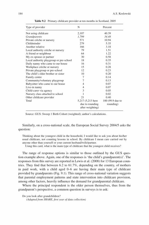
184 A.S. Koslowski
Table 9.2 Primary childcare provider at ten months in Scotland, 2005
Type of provider N Percent
Not using childcare 2,107 40.39Grandparents 1,799 34.48Private creche or nursery 571 10.94Childminder 279 5.35Another relative 166 3.18Local authority creche or nursery 79 1.51A friend or neighbour 64 1.22My ex-spouse or partner 30 0.58Local authority playgroup or pre-school 18 0.35Daily nanny who came to our house 16 0.31Workplace creche or nursery 15 0.28Private playgroup or pre-school 12 0.23The child’s older brother or sister 10 0.20Family centre 7 0.14Community/voluntary playgroup 7 0.13Babysitter who came to our house 4 0.07Live-in nanny 4 0.07Child-carer via agency 3 0.05Nursery class attached to school 1 0.02Other childcare provider 21 0.40Total 5,217 (5,213 here
due to roundingafter weighting)
100 (99.9 due torounding)
Source: GUS: Sweep 1 Birth Cohort (weighted); author’s calculations.
Similarly, on a cross-national scale, the European Social Survey 2004/5 asks thequestion:
Thinking about the youngest child in the household, I would like to ask you about his/herusual childcare, not counting lessons in school. By childcare I mean care carried out byanyone other than yourself or your current husband/wife/partner.
Using this card, what is the main type of childcare that the youngest child receives?
The range of response options is similar to those outlined by the GUS ques-tion example above. Again, one of the responses is ‘the child’s grandparent(s)’. Theresponses from this survey are reported in Lewis et al. (2008) for 13 European coun-tries. They find that between 6.2 to 61.7%, depending on the country, of mothersin paid work, with a child aged 0–6 are having their main type of childcareprovided by grandparents (Fig. 9.1). This range of cross-national variation suggeststhat parental employment patterns and state intervention into childcare provision,among other factors, heavily influence the demand for grandparental childcare.
Where the principal respondent is the older person themselves, thus from thegrandparent’s perspective, a common question in surveys is to ask:
Do you look after grandchildren?(Adapted from SHARE, first year of data collection)

9 Grandparents and the Care of Their Grandchildren 185
70
60
50
40
30
20
10
0
Per
cen
tag
e p
rovi
sio
n
Gre
ece
Bel
gium
Aus
tria
Net
herla
nds
Por
tuga
l
Ger
man
y
Irel
and
Gre
at B
ritai
n
Spa
in
Tot
al
Fin
land
Den
mar
k
Fra
nce
Sw
eden
Country
Fig. 9.1 Childcare provided by grandparents by country(Sources: ESS and calculations of Lewis et al., 2008)
From this question, it is found that many grandparents across Europe look aftertheir grandchildren; grandfathers and grandmothers alike (Table 9.3). The preva-lence of grandparental childcare by this measure varies across countries and acrossages, with peaks between 60–65 years. Women are more likely to care for grand-children than men (Table 6.3). In particular, younger grandparents display notice-able gender differences in the patterns of caring for grandchildren, with grand-mothers taking the lion share (Croda and Gonzalez-Chapela, 2005 – not shown intable).
Hours spent looking after grandchildren are obtained by asking, firstly, how fre-quent these activities are, and then the number of usual hours spent on the activityin a given period of time. On average, Europeans over fifty years of age devote
Table 9.3 Prevalence of caring for grandchildren by gender and country
SE DK DE NL FR CH AT IT ES GR
Grandmothers 34.7(1.5)
39.8(1.8)
24.7(1.3)
34.9(1.5)
35.0(1.7)
21.5(1.9)
26.9(1.3)
25.7(1.9)
27.1(1.7)
25.7(1.4)
Grandfathers 24.4(1.4)
31.1(1.8)
20.7(1.2)
32.0(1.5)
28.9(1.8)
17.3(1.8)
24.7(1.5)
18.8(1.7)
20.5(1.7)
18.7(1.4)
All grandparents 30.0(1.1)
35.8(1.3)
22.9(0.9)
33.6(1.1)
32.2(1.3)
19.5(1.3)
25.9(1.3)
22.7(1.0)
24.3(1.2)
22.5(1.0)
Sample of all older persons is 17,629 un-weighted observations using Version 0 release of SHAREdata. All figures are weighted. Figures refer to whole population of older persons having grand-children. Standard errors are in parentheses.Source: Adapted from Croda and Gonzalez-Chapela (2005, Table 5A.17).

186 A.S. Koslowski
half an hour a day to looking after grandchildren. A clear geographical gradient isobserved for the amount of time devoted to looking after grandchildren: the averageamount increases as we move south (Croda and Gonzalez-Chapela, 2005). Datafrom the Multinational Time Use Study, between 1987 and 1992, have also beenused to calculate average grandparental time. For nine countries, Austria, Canada,Finland, Germany, Italy, the Netherlands, Sweden, the United Kingdom, and theUnited States, time devoted to childcare has been found to be very small, around0.1 to 0.2 hours per day, tending to be slightly higher for women than for men,and for younger (in this case aged 45–54) rather than older women (Gauthier andSmeeding, 2003). This result may be likely to be partly related to the mode of datacollection. Childcare may be performed on an irregular basis and so it may be thatdiary surveys, which typically cover only one randomly selected day, are not bestsuited to capture a non-daily activity. It may also be the result of an averaging effectacross a heterogeneous population.
To the contrary, the 1998 British Social Attitudes (BSA) study asked all sam-ple members some broad questions about the role of grandparents and discov-ered a remarkable level of homogeneity across the sample. “Manifestly, there isa grand-parenting culture which is shared by the majority of people in Britishsociety” (Dench and Ogg, 2002, p. 13). In the BSA study 35% of grandparentsreported often spending the day and overnight (38%) with their grandchildren with-out the parents. Only 28% had not spent such a day within the past year (Denchand Ogg, 2002, p. 22). Grandparents with grandchildren under the age of 12 werealso asked about their role in childcare. Twenty-two per cent reported helping withdaytime childcare on a weekly basis or more. Fifty-three per cent helped with day-time childcare at least weekly. Forty-two per cent helped with evening childcareat least monthly. Eighteen per cent took a grandchild to school or nursery at leastmonthly.
In summary, the available data on grandparental care from the perspective of theolder person can be disappointingly lacking in detail and fail to highlight the intenseactivity identified by studies from the perspective of the grandchild or parent. Whilstthere is a degree of harmonisation across some studies, cross-survey comparisonmay be beleaguered by variations in question wording and sample nature. How-ever, a picture of grandparental care is beginning to be built up. Many grandparentshave regular contact with their grandchildren, but this does not necessarily equate tosubstantial amounts of grandparental childcare time. However, a large minority areheavily involved as the main informal childcare providers, most often in relation toenabling the labour market participation of the mothers.
Conclusion
A review of current literature confirms that in most West European countries, grand-parents are a very important source of childcare. Whilst some grandparents arenot involved in grandparental care a substantial minority do provide considerableamounts of early-years childcare provision. Cross-national variation in the extent to

9 Grandparents and the Care of Their Grandchildren 187
which grandparents are involved in such informal childcare provision suggests thatthere is much that governments can do should their aim be to aid grandparents andparents.
Despite the current emphasis of EU-level policy on enhancing the formal pro-vision of childcare to facilitate the labour market activation of mothers as partof the EU-Lisbon strategy, there is very little evidence of the care activation offathers. Partly as a consequence, the role of grandparents in providing informalchildcare thus remains important in all but the Nordic countries (Lewis et al.,2008). Evidence from the birth cohort studies and the UK Time Use study sug-gests that reliance on grandparental help may also be a function of the social classof the parents. This suggests that formal private childcare provision may, in effect,price certain mothers out of the market, forcing them to find alternative sources ofchildcare.
That grandparents are a very important source of childcare is potentially in con-tradiction with EU policy on ‘active ageing’ (EC, 2002). The amount of hours spentlooking after grandchildren are such that if it were not provided by grandparentsbut rather bought in the marketplace, the economic value of this activity would beconsiderable (Croda and Gonzalez-Chapela, 2005). Furthermore, if grandparentsincreasingly engage with the labour market, then the demand for childcare provi-sion would most likely further outstrip supply. As such, the role of grandparents ascare providers warrants more recognition in policy development.
It is important to move away from the stereotypical grandparent image of a veryold, inactive person. Many grandparents will themselves be juggling employmentand family commitments. Others may just have settled into what they hope will bean active retirement involving leisure pursuits, travel and volunteering work. Thereis much heterogeneity amongst the population of grandparents, which remainslargely unexplored. Studies of ageing fail to capture data on younger grandparents.Birth cohort studies fail to capture contextual information about the grandparents.More reflection is called for as to how best to obtain data on grandparental activityacross the population.
Grandparental time spent on childcare is gendered. Grandmothers are more likelythan grandfathers to be providing informal childcare provision. When grandparentsprovide childcare, this has implications for their financial circumstances as well asfor their economic planning for later life. Further work is needed to estimate thefinancial costs to the older person of grandparental childcare. It is likely that thelifetime disadvantage with regard to earnings of informal care is compounded ifwomen are involved in childcare not once, but twice, and possibly thrice over thelife course.
For both theoretical and policy reasons, it is important to deepen our understand-ing of this population of grandparental carers and the contribution they make toinformal childcare. Many grandparents may be willing to provide care for theirgrandchildren, but this willingness is unlikely to be open-ended. Furthermore, itmay not be sustainable (Dench et al., 1999). More research is called for into theinformal care provision by grandparents for grandchildren and implications of thisactivity for all involved.

188 A.S. Koslowski
References
Age Concern (2004) The Economic Contribution of Older People, Age Concern England PolicyUnit, London.
Age Concern (2006) Grandparents, Age Concern Policy Position Papers, Age Concern EnglandPolicy Unit, London.
Anderson, S., Bradshaw, P., Cunningham-Burley, S., Hayes, F., Jamieson, L., MacGregor, A.,Marryat, L. and Wasoff, F. (2007) Growing up in Scotland: Sweep 1 Overview Report, ScottishExecutive, Edinburgh.
Bamford, C., Gregson, B., Farrow, G., Buck, D., Dowswell, T., McNamee, P., Bond, J. and Wright,K. (1998) Mental and physical frailty in older people: the costs and benefits of informal care,Ageing and Society, 18(3): 317–354.
BBC3 (2008) Britain′s Youngest Grannies, Part of the Seriously Young Season, Film produced byBBC3 programmes.
Bolin, K., Lindgren, B. and Lundborg, P. (2007) Your next of kin or your own career? Caring andworking among the 50+ of Europe, Tinbergen Institute Discussion Paper, TI 2007-032/3.
Bradshaw, P., Jamieson, L. and Wasoff, F. (2008) Growing up in Scotland Study: Use of InformalSupport by Families with Young Children, Scottish Government, Edinburgh.
Brennan, D. and Cass, B. (2007) Understanding grandparent care: Policy and practice implica-tions of grandparents as primary carers of their grandchildren in the Australian context, Paperpresented at the CRFR Extended and Extending Families Conference, University of Edinburgh,27–29 June.
Broad, B. (2004) Kinship care for children in the UK: messages from research, lessons for policyand practice, European Journal of Social Work, 7(2): 211–227.
Budig, M. and Folbre, N. (2004) Activity, Proximity or Responsibility? Measuring Parental Child-care Time, Chapter 3 in Folbre, N. and Bittman, M. (eds.) Family Time: The Social Organizationof Childcare, Routledge, London and New York.
Castles, F. (2004) The Future of the Welfare State: Crisis Myths and Crisis Realities, Oxford Uni-versity Press, Oxford.
Clarke, L. and Cairns, H. (2001) Grandparents and the care of children: the research and evidence,in Broad, B. (ed.) Kinship Care: The Placement Choice for Children and Young People, RussellHouse Publishing, London, pp. 11–20.
Croda, E. and Gonzalez-Chapela, J. (2005) How do European older adults use their time?, inBorsch-Supan, A. (ed.) Health, Ageing and Retirement in Europe – First results from the Surveyof Health, Ageing and Retirement in Europe, Mannheim Research Institute for the Economicsof Aging, Mannheim, pp. 265–271.
Crompton, R. (1999), Restructuring Gender Relations and Employment: The Decline of the MaleBreadwinner, Oxford University Press, Oxford.
Crouch, C. (1999) Social Change in Western Europe, Oxford University Press, Oxford.Daly, M. (2002) A fine balance: Women’s Labor Market Participation in International Comparison,
in Scharpf, F.W. and Schmidt, V.A. (eds.) Welfare and Work in the Open Economy, Vol. II,Oxford University Press, Oxford, pp. 467–510.
Dench, G and Ogg, J. (2002) Grand-parenting in Britain: A Baseline Study, Institute of CommunityStudies, London.
Dench, G., Ogg, J. and Thompson, K. (1999) The role of grandparents’, in Jowell, R., Curtice, J.,Park, A. Brook, L. and Thomson, K. (eds.) British Social Attitudes: The 16th Report, Ashgate,Aldershot, pp. 135–157.
Ditch, J., Bradshaw, J. and Eardley, T. (1996) Developments in National Family Policies in 1994,Social Policy Research Unit. York.
Douglas, G. and Ferguson, N. (2003) The role of grandparents in divorced families, InternationalJournal of Law, Policy and the Family, 17(1): 41–67.
EC (1990) 1992 – The Social Dimension. 4th Edition. European Documentation 2/1990, EuropeanCommission, Brussels.

9 Grandparents and the Care of Their Grandchildren 189
EC (2002) Increasing labour force participation and promoting active ageing, COM (2002) 9 final,European Commission, Brussels.
Esping-Andersen, G., Gallie, D., Hemerijck, A. and Myles, J. (2002) Why We Need a New WelfareState, Oxford University Press, Oxford.
Gauthier, A. and Smeeding, T. (2003) Time use at older ages: cross-national differences, Researchon Aging, 25(3): 247–274.
Gershuny, J. (2004) Costs and benefits of time sampling methodologies, Social IndicatorsResearch, 67: 247–252.
Gornick, J. and Meyers, M. (2003) Families that Work: Policies for Reconciling Parenthood andEmployment, Russell Sage Foundation, New York.
Grandparents plus and Adfam, (2006) Forgotten Families: The Needs and Experiences ofGrandparents who Care for Children whose Parents Misuse Drugs and Alcohol, Adfam andGrandparents plus, London.
Gray, A. (2005) The changing availability of grandparents as carers and its implications for child-care policy in the UK, Journal of Social Policy, 34(4): 557–577.
Greengoss, Baroness (4 June 2007) Lords Debate, Pensions Bill, Hansard.Hank, K. and Buber, I. (2007) Grandparents caring for their grandchildren: findings from the
2004 Survey of Health, Ageing and Retirement in Europe, MEA Working Paper 127–2007,Mannheim Research Institute for the Economics of Aging, University of Mannheim.
Hansen, K. and Hawkes, D. (2009) Early childcare and child development, Journal of Social Policy,38(2): forthcoming.
Hirshorn, B.A. (1998) Grandparents as caregivers, in Szinovacz, M.E. (ed.) Handbook on Grand-parenthood, Greenwood Press, Westport, pp. 200–216.
Hook, J. (2006) Care in context: men’s unpaid work in 20 countries, 1965–2003, American Socio-logical Review, 71(4): 639–660.
Joshi, H., Paci, P. and Waldfogel, J. (1999) The wages of motherhood: better or worse, CambridgeJournal of Economics, 23: 543–564.
Juster, F.T. and Stafford, F.P. (1991) The allocation of time: empirical findings, behavioral modelsand problems of measurement, Journal of Economic Literature, 29: 471–522.
Kemp, C. (2003) The social and demographic contours of contemporary grandparenthood: map-ping patterns in Canada and the United States, Journal of Comparative Family Studies, 34(2):187–212
Land, H. (2002) Spheres of care in the UK: separate and unequal, Critical Social Policy, 22(1):13–32.
Le Bihan, B. and Martin, C. (2004) Atypical working hours: consequences for childcare arrange-ments, Social Policy and Administration, 38(6): 565–590.
Lee, Y.-S. (2005) Measuring the gender gap in household labor: accurately estimating wives’ andhusbands’ contributions, in Schneider, B. and Waite, L.J. (eds.) Being Together, Working Apart:Dual-Career Families and the Work-Life Balance, Cambridge University Press, Cambridge,pp. 229–247.
Lewis, J., Campbell, M. and Huerta, C. (2008) Patterns of paid and unpaid work in Western Europe:gender, commodification, preferences and the implications for policy, Journal of EuropeanSocial Policy, 18(1): 21–37.
Kroll, B. (2007) A family affair? Kinship care and parental substance misuse: some dilemmasexplored, Child and Family Social Work, 12: 84–93.
OECD (2004) Babies and Bosses – Reconciling Work and Family Life, Volume 3: New Zealand,Portugal and Switzerland, OECD, Paris.
Price, D. (2006) Why are older women in the UK poor? Quality in Ageing, 7(2): 23–32.MacKenzie, P. (2007) The multiple layers of mothering work: grandparents raising grandchil-
dren, Paper presented at the CRFR Extended and Extending Families Conference, Universityof Edinburgh, 27–29 June.
Murphy, M. and Grundy, E. (2003) Mothers with living children and children with living mothers:the role of fertility and mortality in the period 1911–2050, Population Trends, 112: 34–44.

190 A.S. Koslowski
Neilson, J. (1998) European briefing: equal opportunities for women in the European Union: suc-cess or failure, Journal of European Social Policy, 8(1): 64–79.
Richards, A. (2001) Second Time Around: A Survey of Grandparents Raising Their Grandchildren,Family Rights Group, London.
Rowlatt, J. (2007) Current Affairs, BBC – The One Show, URL www.bbc.co.uk/ theoneshow/article/2007/07/jr˙grannynannies.shtml accessed 5 May 2008.
Smith, A. and Williams, D. (2007) Father friendly legislation and paternal time across WesternEurope, Journal of Comparative Policy Analysis, 9(3): 175–192.
Smith Koslowski, A. (2008) Who Cares? European Fathers and the Time they Spend Looking afterChildren, VDM Verlag Dr Muller, Saarbrucken.
Szikra, D. (2008) Personal correspondence with the author, April.Wallace, C. (2002) Household strategies: their conceptual relevance and analytical scope in social
research, Sociology: 36 (2) 275–292.Wheelock, J. and Jones, K. (2002) Grandparents are the next best thing: informal childcare for
working parents in urban Britain, Journal of Social Policy, 31(3): 441–63.

Chapter 10Internal Migration and Inter-householdRelationships
Oliver Duke-Williams
Introduction
Internal migration is an important agent of population change within the UnitedKingdom; it can alter the characteristics of some areas – the balance of differentsorts of people who live there – quite significantly over a short period of time.Like migration, commuting behaviour also causes massive changes to the popu-lation of an area on a temporary (usually daily) basis. Both these agents of change,migration and commuting, are closely linked. Change in usual residential locationinevitably means a change in commuting patterns for those migrants in employment;people may commute to a new job – possibly by a different mode of transport –or they may make a commute over a different, possibly longer, route to the sameworkplace.
Although we associate migration with flows of people, most research has tendedto consider flows of individuals. A relatively little explored aspect of migration isthe groups of people who move together, sometimes in groups, most frequently asa household or a family. Moreover, whilst many people move to a new house orflat in which they are the only occupants, others move into households in whichsome people are already living. There is clearly a relationship between group size(and, perhaps, group behaviour) and household type and the various life stages ofthe people in those households. A single person must, by definition, move on theirown, although he or she may move to form a new relationship in a multi-personhousehold. Young children are likely to move as a part of a family group with theirparent/s, whilst older children may move out of the parental household on their own.Indeed, mobility is a key driver in household changes, as people move and createnew households.
O. Duke-Williams (B)School of Geography, University of Leeds, Leeds LS2 9JT, UKe-mail: o.w.duke–[email protected]
J. Stillwell et al. (eds.), Fertility, Living Arrangements, Care and Mobility, UnderstandingPopulation Trends and Processes 1, DOI 10.1007/978-1-4020-9682-2 10,C© Springer Science+Business Media B.V. 2009
191

192 O. Duke-Williams
Much research has focused on the phenomenon of young people leaving home(Buck and Scott, 1993; Clark and Mulder, 2000; Ermisch, 1999), a process whichis notable for being highly variable in nature in different countries (Aassve et al.,2002). A sub-group of these migrants are students who leave home as individualsto live together in large groups in halls of residence or with small groups in pri-vate households (Duke-Williams, forthcoming). Interest has also focused on shift-ing attitudes towards and age-specific propensities of marriage and cohabitation(Berrington and Diamond, 2000), and the role of separation and divorce in residen-tial mobility (Grundy, 1992). A further avenue for research has been the mobility ofthe elderly (Glaser and Grundy, 1998).
In this chapter, groups of migrants who move together are considered in termsof the general spatial mobility patterns, and the motivations for migration expressedby persons in different groups and in different types of household. The census dataare used to study overall mobility patterns for groups of different sizes and types.A feature of migration data from the 2001 Census was the disaggregation by grouptype and size, resulting in outputs that were often hard to interpret. One reason forstudying differences between groups is to determine whether a disaggregation ofthis sort is always necessary.
The chapter commences by outlining two data sources that are used in the anal-ysis: the 2001 Census Special Migration Statistics (SMS) and the British House-hold Panel Study (BHPS). Data from the 2001 Census are then used to examinemovement patterns by migrants in groups of different sizes and to consider whetherthere is anything distinctive in the difference between wholly moving households(where all persons in a household are migrants and had the address one yearbefore the census) and migrants in other groups. A series of connectivity indicesare produced for migrants in groups of different sizes and of different types, forboth origin and destination specific flows. Correlation coefficients are then exam-ined in order to investigate the similarity in connectivity levels for all districts fordifferent groups. Connectivity indices are used as a simple metric for comparingoverall levels of migration in a system. They have the advantage that no popula-tions at risk (PAR) are required to produce a summary statistic. This is significant,because the PAR for group level migration are unclear: who is at risk of becominga singleton migrant? All people? People who live on their own? There is no clearanswer.
Having examined patterns at the group level, the focus is then changed tothe household level. Data from the BHPS – a panel study – are used to com-pare expectations of migration with actual behaviour in two ways. Firstly, theactual process of migration is considered: where people expressed some degreeof desire to migrate, did they actually do so in the following year? Secondly,for those people that did migrate, what were their reasons for doing so? Thisanalysis is disaggregated on a household type basis: one might expect peoplein different household types to have different reasons for moving, but is thisactually the case? Finally, a comparison is made of spatial and social mobility.Recording of social class of migrants allows a determination to be made of thedegree to which migrant’s social status changes around the same time that theymove.
10 Internal Migration and Inter-household Relationships 193
Data Sources
Data from the 2001 Census interaction data sets have been used to explore somegeneral patterns of the way that people move around the country. The 2001 Censusinteraction data continued a series of similar data from earlier censuses, but arecollectively larger and more complex than those that preceded them (Rees et al.,2002; Cole et al., 2002). Three sets were produced – the Special Migration Statistics(SMS), the Special Workplace Statistics (SWS) and the Special Travel Statistics(STS) – at three spatial scales. Whereas the SMS provide UK-wide spatial coverage,the other two sets are spatially constrained. The STS were generated for residencesin Scotland only, while the SWS were produced for residences elsewhere in theUK. The STS are effectively a superset of the SWS for flows with destinations inScotland, in that they include both journeys from home to work (as do the SWS)and journeys from home to a place of study for full-time students (including schoolchildren).
The interaction or origin-destination data were produced at three spatial scalesreferred to as levels. Level 1 refers to the local authority districts across GreatBritain – an amalgam of different types of local government authorities in England,Wales and Scotland – together with parliamentary constituencies in NorthernIreland. Level 2 involves ward level data and contains an amalgamation of censusarea statistics (CAS) wards in England, Wales and Northern Ireland, and standardtable (ST) wards in Scotland. The combinations of component geographies used inthese two levels are distinct to the interaction data, and are respectively referred toas ‘interaction data districts’ and ‘interaction data wards’. Level 3 spatial units areoutput areas, a new geography created for the outputs of the 2001 Census (Martin,2002). The set of areas used for the interaction data are equivalent to those areasused for other census outputs.
Across all three sets of interaction data, results are presented in a variable num-ber of cross-aggregated tables. The number of tables available, and the numbers ofcategories used in component variables varies with spatial scale: at level 1 there aremore tables, with finer classifications used and at level 2, there are fewer tables withcoarser classifications (Stillwell and Duke-Williams, 2007). For both SMS and theSWS/STS, there is only a single table available at level 3, the finest spatial scale: anage by sex table in the case of the SMS and a mode of travel table in the case of theSWS and STS.
In contrast to the 2001 Census, the BHPS can be used to explore connectionsbetween household structure and migration events. The BHPS is a panel study thatcommenced in 1991 and has been updated with annual survey waves since then.As a panel study, it follows the same groups of individuals over time. A distinctfeature of the BHPS is that it is household based, with all adult members of surveyhouseholds being interviewed, and children aged 11+ also completing a short inter-view. The survey is a multi-purpose study with core and additional elements cov-ering many areas including social attitudes, employment and income, housing andtenure, health, relationship histories, and individual and household demographics.The survey also includes questions on residential mobility, which are explored inthis chapter.

194 O. Duke-Williams
The initial panel consisted of over 5,000 households containing over 10,000individuals, and this panel has grown over time through the inclusion of additionalsamples in Scotland, Wales and Northern Ireland. The panel accumulates new mem-bers as a result of mobility: when a sample member moves to a new household, themembers of that household also become sample members. However, mobility is alsoa major cause of sample attrition, as panel members cannot always be traced; otherlosses include refusal to be interviewed. By wave 13, the total number of personsinterviewed had fallen to 8,655 (Lynn, 2006).
General Patterns of Migration
The 2001 Census interaction data provide useful information about migration andcommuting within the UK. They have particular strengths over sample studies inthat they include the whole population. This is of particular significance with a phe-nomenon such as migration, because ‘migrants’ are a relatively small sub-set ofthe whole population: about 10% of the UK population were internal migrants bythe Census definition in the period 2000–2001. Persons are defined as migrants bythe 2001 Census if they have changed their usual residence in the year prior to theCensus. The propensity to migrate varies with various socio-demographic charac-teristics (Champion, 2005), the most notable of which is age. Figure 10.1 showsthe numbers of internal migrants in the UK per 1,000 persons, by quinary agegroups. The distribution is a typical one for migration, with the highest rates beingfound amongst young adults. Rates are also relatively high for the elderly, and for
Male Female350
300
250
200
150
100
50
0
Mig
ran
ts p
er 1
,000
per
son
s
Age group
0–4
5–9
10–1
4
15–1
9
20–2
4
25–2
9
30–3
4
35–3
9
40–4
4
45–4
9
50–5
3
55–5
9
60–6
4
65–6
9
70–7
4
75–7
9
80–8
4
85–8
9
90+
Fig. 10.1 Internal migration rates by age, UK, 2000–2001(Source: 2001 Census SMS l; author’s calculations.)

10 Internal Migration and Inter-household Relationships 195
young children. Another characteristic of migration illustrated in Fig. 10.1 is thatunlike many other social phenomena, overall migration propensities in countrieslike the UK exhibit little gender difference. Further analysis of age and gender vari-ations in the 12 months before the 2001 Census is available in Dennett and Stillwell(forthcoming).
The term ‘migration’ covers a variety of types of mobility, from persons mov-ing on their own to groups of several persons moving together. In censuses prior tothe 2001 Census, a distinction was drawn between ‘wholly moving households’ and‘other groups of migrants’. The term wholly moving household refers to a house-hold in which all persons were migrants and all had the same usual residence oneyear prior to the census; the definition encompasses persons who have moved assingletons. The term does not necessarily mean that all persons who were in theoriginal household moved – it may be the case that one or more persons remainedin that household, and this might particularly be the case with singletons when, forexample, a young adult has moved out of their parental home and into their ownaccommodation. It might be possible to identify truly ‘wholly moving’ cases (thatis, where all persons in the original household have moved together) using originalcensus data, but such analysis would be complicated and expensive, and probablyprone to error.
Table 10.1 illustrates the changes observed in the number of wholly mov-ing households in Great Britain in the 1991 and 2001 Censuses. The number ofwholly moving households, and the number of migrants contained within themboth increased when the two censuses are compared. This apparent increase shouldbe understood in the context of changes in both the census base population, andthe handling of migrants from an unstated origin. The 2001 Census included stu-dents at their term-time residence rather than at their parental residence, as wasthe case in 1991; this may have affected either their household residency status, ortheir membership of wholly moving households. In addition, as part of the 2001Census processing, migrants’ origins that were missing or not fully stated wereimputed, whereas in the 1991 SMS, they were tabulated separately. No migrants
Table 10.1 Numbers of wholly moving households and migrants in Great Britain, 1990–1991 and2000–2001
1990–1991 2000–2001
Number of migrants in households 4,463,974 5,670,422Number of wholly moving households 1,366,115 1,665,469Migrants in wholly moving households 3,085,854 3,451,938Mean number of migrants per wholly
moving household2.3 2.1
% of migrants in households 69 61
Sources: 1991 Census SMS Set 2, Table 2; 1991 Census SMSGAPS Table 6; 2001 Census SMSLevel 1, Table 6.

196 O. Duke-Williams
with unstated origins were coded as being in ‘wholly moving households’ in 1991,whereas migrants in 2001 with imputed origins could have been coded as being inwholly moving households.
Table 10.1 also shows the mean number of migrants in each wholly mov-ing household, and the percentage of all migrants in households who were clas-sified as being in wholly moving households. Despite the apparent increase inthe number of migrants in wholly moving households between 1991 and 2001,the mean number of migrants per group had fallen, as had the percentage of allmigrants that were in wholly moving households. It is possible that the decreasein mean group size is a result of significant numbers of migrants with imputedorigins being coded as single person wholly moving households. However, thedistribution of group sizes was not published for 1991 data, so this explanationremains speculative. The decrease in the proportion of migrants who were in whollymoving households may be related to improved capture of data relating to stu-dents, and the growth in the period of the numbers of students living in sharedhouseholds.
The 2001 Census processing introduced an additional way of classifying groupsof migrants: that of the moving group. A moving group is a group of persons whowere migrants and had the same usual residence one year prior to the census. Awholly moving household, using the previous definition, is thus one example of atype of moving group. However, the classification also includes non-wholly movinggroups; these include the cases where:
• one or more persons in the household is a migrant but not all household membersare; and
• all persons in the household are migrants but do not all have the same usualresidence one year prior to the census.
Identification of moving groups at the time of census processing was exhaus-tive: that is, all migrants in households were allocated to a moving group.Table 10.2 shows the national distribution of migrants in households (as opposedto communal establishments) according to their group status. The ‘one per-son’ counts are the same for groups and for migrants for both wholly mov-ing households and other moving groups. There were approximately 5.8 millionpersons within the UK in 2000–2001 migrating in 3.5 million moving groups,of which 48% were wholly moving households and 52% were ‘other mov-ing groups’. A very high proportion of those persons moving in other movinggroups were in fact individual movers (85%) compared to 42% of wholly movinghouseholds.
Amongst the 3.5 million persons migrating in wholly moving households, overhalf involved three or more persons moving together, with 28.3% in two personhouseholds and one fifth as single persons. In contrast, over two thirds of migrantsin other moving groups were single persons, with similar numbers split between twoperson and three or more person groups.

10 Internal Migration and Inter-household Relationships 197
Table 10.2 Groups and migrants within the UK, 2000–2001
Number of persons
1 person 2 persons 3+ persons All
Wholly moving households
Groups 719,379 500,461 486,356 1,706,196Migrants 719,379 1,000,922 1,821,914 3,542,215
Other moving groups
Groups 1,545,286 178,041 104,753 1,828080Migrants 1,545,286 356,082 367,029 2,268,397
Source: 2001 Census SMS level 1, Table 6.
Migration Connectivity
The results shown in Tables 10.1 and 10.2 indicated that whilst the majority ofmigrants are in wholly moving households, there are a very significant number whoare in sub-household size groups. Table 10.1 suggested that the proportion in whollymoving households may have fallen between 1991 and 2001, although changes tothe population base and the way in which migrants with an unstated origin were pro-cessed mean that this interpretation must be cautious. An obvious question arises: domigrants in different sorts of groups (both in terms of size, and in terms of whetherthe group formed a wholly moving household or not) have different mobility pat-terns? If they do, then the distinction offered in the 2001 Census between differentsorts of groups is a useful and important one; if they do not then disaggregation bygroup type and size is an unnecessary complication of the output tables that wouldserve only to confuse users.
In order to compare the characteristics of migrants at a national scale in dif-ferent groups, connectivity indices (Bell et al., 2002) were constructed for whollymoving groups, and for other groups which did not form a wholly moving house-hold. Index values were calculated for all groups at the district level. A connectivityindex is a simple measure that shows the extent to which any one place is con-nected to other places through migration. If the index for any location is equalto 1.0, then that place is connected to all other places in the universe of inter-est (that is, it has a non-zero observed flow to or from all other locations); if theindex has a value of 0.0 then that location is connected to no other places. Sep-arate sets of indices were constructed from an origin perspective and from a des-tination perspective. A high origin-specific index means that the location sendsmigrants to a large number of other locations, and a high destination-specificindex indicates that the location receives migrants from a large number of otherlocations. The index value is dependent on the spatial scale for which it is con-structed: the coarser the geography, the higher the index values will be. However,given a fixed geographic scale, it provides a simple mechanism for comparing flowcharacteristics.

198 O. Duke-Williams
0.00 – 0.130.14 – 0.190.20 – 0.270.28 – 0.00
One personhousehold
0.00 – 0.130.14 – 0.190.20 – 0.270.28 – 0.00
Two personhousehold
0.00 – 0.130.14 – 0.190.20 – 0.270.28 – 0.00
Three or moreperson household
Fig. 10.2 Migration destination connectivity index values for wholly moving households;2000–2001 (a) Single person households (b) Two person households (c) Three or more personhouseholds(Source: Author’s analysis based on census data.)
Figure 10.2 shows the values of the destination-specific connectivity index forwholly moving households consisting of (a) one person, (b) two people and (c)three or more persons. The shading scheme is different for each map, and in eachcase is based on result quartiles: the darkest shaded areas are the 25% of dis-tricts with the highest destination-specific connectivity values. In absolute terms,there is a steady decline in connectivity as the group size increases: connectivi-ties are higher for single person households than for two person households, andin turn, connectivities are higher for two person households than for three personhouseholds. Two features are apparent in this set of maps. Firstly, districts in Scot-land have high connectivity values, and secondly, the spatial pattern elsewhere isvariable.
The high levels for Scottish Council Areas are in part an artefact of the sta-tistical disclosure control methods applied to the interaction (and other census)data, although some Scottish destinations are popular of course and thus well con-nected to other locations. The data were subject to a statistical disclosure controlmethod termed SCAM, the small cell adjustment methodology (Duke-Williams andStillwell, 2007). Small values (the definition of small was not disclosed by the cen-sus agencies but was widely understood to be the values 1 and 2) in the originaldata were modified to become either value 0 or 3. However, this procedure wasnot followed in Scotland, including those parts of the SMS that related to destina-tions in Scotland. Thus, a significant number of small flows (which might otherwise

10 Internal Migration and Inter-household Relationships 199
have been changed to 0) remained present in the data relating to Scotland, withthe result that more distinct flows were observed in the published data for Scottishdestinations.
The patterns of destination connectivity outside Scotland are not affected in thisway, and are thus of more direct interest. The maps shown in Fig. 10.2 show a shift-ing pattern of destination preference given group size. A good example of this isfor London and the surrounding area – this has high connectivity values for sin-gle person households: people who were living on their own at the time of the2001 Census, and had been migrants in the preceding year, had moved there froma wide range of origin districts. This is less marked for two person households, andthere is a low connectivity ‘hole’ around London for wholly moving householdsof three or more persons. This finding indicates that people in larger wholly mov-ing households moved to the London area from a limited set of origins; it doesnot necessarily indicate a difference in the absolute numbers of households or per-sons involved. Another visual effect that is clear on the map is that the darkestshaded areas appear to take up more space for the larger groups. This is because theareas in the highest connectivity quartile are larger less urban districts. The inverseof this is less immediately visually obvious: that for single person households,those districts with the highest connectivity index values tend to be small urbandistricts.
In order to determine the extent to which flow patterns differed by group size, bywholly or partly moving status, and by origin or destination specificity, correlationcoefficients were calculated for various sets of migration connectivity indices. Ahigh coefficient indicates that the pairs of connectivity indices are similar: that eachzone under consideration dispatches (or receives) migrants from a similar numberof areas. Thus, if the connectivity indices have a high correlation, those areas inthe first group that are highly connected are also highly connected in the secondgroup, whilst those areas that are poorly connected in the first group are also poorlyconnected in the second group. It does not necessarily mean that each pair of areasbeing compared are connected to the same partner areas.
Table 10.3 shows the correlation coefficients for each pair of origin-specificmigration connectivity indices. Comparisons are made for all groups (i.e., one per-son against two persons, one person against three plus persons and two personsversus three plus persons) within the wholly and partly moving sets, and for eachsame-size group where wholly and partly moving groups are compared. Compar-isons within each ‘family’ (‘wholly moving households’ or ‘other groups’) explorethe effect of group size on behaviour, accounting for any wholly or partly movingdifferences; comparisons between these families explore the effect of wholly ver-sus partly moving status whilst accounting for group size. The correlations for theorigin-specific values are lowest (suggesting different patterns of movement) withinthe sets of ‘other groups’ – those who did not form wholly moving households. Thissuggests a difference in origin connectivity for these ‘other groups’: areas that arehighly connected (that is, distribute migrants to a large number of destinations) forsingle persons, are not necessarily highly connected for larger groups. This differ-ence is most marked when single person groups are compared with groups of three

200 O. Duke-Williams
Table 10.3 Comparison of correlation coefficients for origin-specific values
Wholly movinghouseholds Other groups
1 2 3+ 1 2 3+
Wholly moving 1 person – 0.94 0.88 0.94 – –households 2 persons – 0.93 – 0.90 –
3+ persons – – – 0.87
Other groups 1 person – 0.87 0.742 persons – 0.883+ persons –
Source: Author’s analysis based on census data.
or more persons. The indices are more strongly correlated for wholly moving house-holds: areas that are strongly connected for single persons also tend to be stronglyconnected for larger groups.
Equivalent results are shown for destination-specific connectivity indices inTable 10.4. Almost all coefficient values are lower for the destination-specific indexcomparisons than for the equivalent comparisons amongst origin-specific values.This suggests greater variation by group size and by wholly/partly moving statuswhen migration is viewed from the destination perspective – areas that are stronglyconnected as destinations (that is, they receive migrants from many other districts)are not necessarily strongly connected if the group size or type changes. This ismost marked for the comparison of wholly moving households, in particular forsingle person households in comparison to households of three or more persons.
The final set of correlation coefficients are shown in Table 10.5. These showthe comparisons of origin versus destination-specific values for fixed group sizeand group type. The coefficient values decrease with group size for both grouptypes, indicating that the larger the group size, the greater the difference in originand destination-specific patterns. Given that the origin-specific values have a strongwithin-type correlation, this suggests that destination choice is more selective asgroup size increases.
Table 10.4 Comparison of correlation coefficients for destination specific values
Wholly movinghouseholds Other groups
1 2 3+ 1 2 3+
Wholly moving 1 person – 0.74 0.64 0.90 – –households 2 persons – 0.86 – 0.67 –
3+ persons – – – 0.73
Other groups 1 person – 0.88 0.702 persons – 0.813+ persons –
Source: Author’s analysis based on census data.
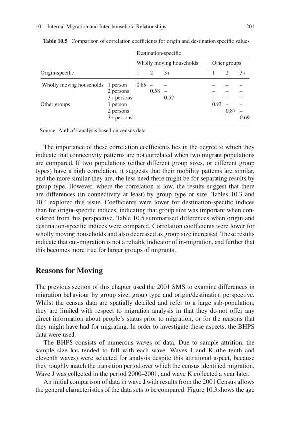
10 Internal Migration and Inter-household Relationships 201
Table 10.5 Comparison of correlation coefficients for origin and destination specific values
Destination-specific
Wholly moving households Other groups
Origin-specific 1 2 3+ 1 2 3+
Wholly moving households 1 person 0.86 – – – – –2 persons 0.58 – – – –3+ persons 0.52 – – –
Other groups 1 person 0.93 – –2 persons 0.87 –3+ persons 0.69
Source: Author’s analysis based on census data.
The importance of these correlation coefficients lies in the degree to which theyindicate that connectivity patterns are not correlated when two migrant populationsare compared. If two populations (either different group sizes, or different grouptypes) have a high correlation, it suggests that their mobility patterns are similar,and the more similar they are, the less need there might be for separating results bygroup type. However, where the correlation is low, the results suggest that thereare differences (in connectivity at least) by group type or size. Tables 10.3 and10.4 explored this issue. Coefficients were lower for destination-specific indicesthan for origin-specific indices, indicating that group size was important when con-sidered from this perspective. Table 10.5 summarised differences when origin anddestination-specific indices were compared. Correlation coefficients were lower forwholly moving households and also decreased as group size increased. These resultsindicate that out-migration is not a reliable indicator of in-migration, and further thatthis becomes more true for larger groups of migrants.
Reasons for Moving
The previous section of this chapter used the 2001 SMS to examine differences inmigration behaviour by group size, group type and origin/destination perspective.Whilst the census data are spatially detailed and refer to a large sub-population,they are limited with respect to migration analysis in that they do not offer anydirect information about people’s status prior to migration, or for the reasons thatthey might have had for migrating. In order to investigate these aspects, the BHPSdata were used.
The BHPS consists of numerous waves of data. Due to sample attrition, thesample size has tended to fall with each wave. Waves J and K (the tenth andeleventh waves) were selected for analysis despite this attritional aspect, becausethey roughly match the transition period over which the census identified migration.Wave J was collected in the period 2000–2001, and wave K collected a year later.
An initial comparison of data in wave J with results from the 2001 Census allowsthe general characteristics of the data sets to be compared. Figure 10.3 shows the age
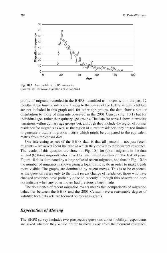
202 O. Duke-Williams
80
70
60
50
40
30
20
10
0
Mig
rati
on
fre
qu
ency
Age100806040200
Fig. 10.3 Age profile of BHPS migrants(Source: BHPS wave J; author’s calculations.)
profile of migrants recorded in the BHPS, identified as movers within the past 12months at the time of interview. Owing to the nature of the BHPS sample, childrenare not included in this graph and, for other age groups, the data show a similardistribution to those of migrants observed in the 2001 Census (Fig. 10.1) but forindividual ages rather than quinary age groups. The data for wave J show interestingvariations within quinary age groups but, although they include the region of formerresidence for migrants as well as the region of current residence, they are too limitedto generate a usable migration matrix which might be compared to the equivalentmatrix from the census data.
One interesting aspect of the BHPS data is that all persons – not just recentmigrants – are asked about the date at which they moved to their current residence.The results of this question are shown in Fig. 10.4 for (a) all migrants in the dataset and (b) those migrants who moved to their present residence in the last 30 years.Figure 10.4a is dominated by a large spike of recent migrants, and thus in Fig. 10.4bthe number of migrants is shown using a logarithmic scale in order to make trendsmore visible. The graphs are dominated by recent moves. This is to be expected,as the question refers only to the most recent change of residence; those who havechanged residence have probably done so recently, although this observation doesnot indicate when any other moves had previously been made.
The dominance of recent migration events means that comparisons of migrationbehaviour between the BHPS and the 2001 Census have a reasonable degree ofvalidity: both data sets are focused on recent migrants.
Expectation of Moving
The BHPS survey includes two prospective questions about mobility: respondentsare asked whether they would prefer to move away from their current residence,

10 Internal Migration and Inter-household Relationships 203
1600
1400
1200
1000
800
600
400
200
0
Nu
mb
er o
f sa
mp
le p
erso
ns
Year moved to present address
200019901970196019401930 1950 1980
10,000
1000
100
10
1
Nu
mb
er o
f sa
mp
le p
erso
ns
Year moved to present address
200019951985198019751970 1990
All migrants
Detail of 1970 onwards, log scale
Fig. 10.4 Year moved to present address by BHPS migrants (a) All migrants (b) detail 1970onwards, log scale(Source: BHPS wave J; author’s calculations.)
and also whether they expect to move within the next 12 months. Table 10.6 showsthe separate and joint responses for these two questions. Of all persons with a validanswer, 33% indicated that they would prefer to move house. However, there areobvious constraints to mobility including occupational, domestic and social ties aswell as financial considerations which mean that a general desire does not necessar-ily mean that a person really intends to move. Of the same respondents, 14% saidthat they expected to move within the next 12 months. The main part of Table 10.6shows the expectations of persons with different preferences: of all those who pre-ferred to move, 64% did not in fact expect to move. There was closer correlation, asmight be expected, for non-movers: of those who preferred to stay where they were,91% did not expect to move within the next 12 months.
Preference for a move varies by many characteristics, including age and house-hold type. Table 10.7 summarises the proportions of persons expressing a prefer-ence for moving by gender and household type, for four age groups. In each row,

204 O. Duke-Williams
Table 10.6 Preference for and expectation of moving
Expect to move
Prefer to move? Don’t know (4%) Yes (14%) No (82%) Total (100%)
Don’t know (1%) 19% 18% 63% 191Stay here (66%) 2% 6% 91% 9,915Prefer to move (33%) 8% 29% 64% 4,975Total 641 2,073 13,367 15,081
Source: BHPS wave J; author’s calculations.
Table 10.7 Preference for moving
Age group
Prefer to stay All ages 16–24 25–44 45–64 65+% % % %
By genderMale 7,177 57 54 66 78Females 8,426 54 58 69 79
By household typeSingle non-elderly∗ 1,085 55 50 62 67Single elderly∗ 1,237 – – 75 84Couple: no children 4,406 53 – 73 79Couple with dependent children 4,563 60 60 70 90Couple with non-dependent children 1,839 57 56 71 82Lone parent with dependent children 795 53 52 57 64Lone parent with non-dependent children 536 66 50 69 852+ unrelated adults 356 58 54 52 80Other households 262 47 50 68 72
∗ - ‘Elderly’ is gender-specific retirement age. A small number of persons are mis-coded aselderly when aged 64, and as non-elderly when aged 65.Source: BHPS wave J; author’s calculations.
the table shows the percentage of persons in that category (male, female, et cetera)of that age group, who indicated a preference to stay. All persons in all householdsare included in this comparison. An ‘all ages’ base is shown for each category, indi-cating that the numbers of persons in each age group vary by category. In all cases,the strongest preference for staying is found amongst the oldest age group, and inmost cases the lowest preference for staying is found in the age group 25–44. Thehighest preference for staying across all ages is found for persons in a couple familywith dependent children.
Realisation of Expectation
The results described above were obtained by studying a single wave of the BHPSdata. By linking more than one wave of panel data, it is possible to study changes
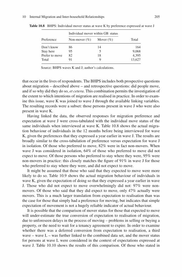
10 Internal Migration and Inter-household Relationships 205
Table 10.8 BHPS: Individual mover status at wave K by preference expressed at wave J
Individual mover within GB status
Preference Non-mover (%) Mover (%) Total
Don’t know 86 14 164Stay here 95 5 9,068Prefer to move 82 18 4,395Total 91 9 13,627
Source: BHPS waves K and J; author’s calculations.
that occur in the lives of respondents. The BHPS includes both prospective questionsabout migration – described above – and retrospective questions: did people move,and if so why did they do so, et cetera. This combination permits the investigation ofthe extent to which intentions of migration are realised in practice. In order to exam-ine this issue, wave K was joined to wave J through the available linking variables.The resulting records were a subset: those persons present in wave J who were alsopresent in wave K.
Having linked the data, the observed responses for migration preference andexpectation at wave J were cross-tabulated with the individual move status of thesame individuals when interviewed at wave K. Table 10.8 shows the actual migra-tion behaviour of individuals in the 12 months before being interviewed for waveK, given the preferences that they expressed a year earlier in wave J. The results arebroadly similar to the cross-tabulation of preference versus expectation for wave Jin isolation. Of those who preferred to move, 82% were in fact non-movers. Whenwave J was considered in isolation, 64% of those who preferred to move did notexpect to move. Of those persons who preferred to stay where they were, 95% werenon-movers in practice: this closely matches the figure of 91% in wave J for thosewho preferred to stay where they were, and did not expect to move.
It might be assumed that those who said that they expected to move were morelikely to do so. Table 10.9 shows the actual migration behaviour of individuals inwave K, given the expectation of doing so that they expressed a year earlier in waveJ. Those who did not expect to move overwhelmingly did not: 97% were non-movers. Of those who said that they did expect to move, only 47% actually weremovers. This is a much larger translation from expectation to realisation than wasthe case for those that simply had a preference for moving, but indicates that simpleexpectation of movement is not a hugely reliable indicator of actual behaviour.
It is possible that the comparison of mover status for those that expected to movewill under-estimate the true conversion of expectation to realisation of migration,due to unforeseen delays in the process of moving – problems in selling or buying aproperty, or the need to wait for a tenancy agreement to expire. In order to examinewhether there was a deferred conversion from expectation to realisation, a thirdwave – wave L – was further linked to the combined data set, and the mover statusfor persons at wave L were considered in the context of expectations expressed atwave J. Table 10.10 shows the results of this comparison. Of those who stated in

206 O. Duke-Williams
Table 10.9 BHPS: Individual mover status at wave K by expectation expressed at wave J
Individual mover status
Expectation Non-mover (%) Mover within GB (%) Total
Don’t know 86 14 561Yes 53 47 1,679No 97 3 11,387Total 91 9 13,627
Source: BHPS waves K and J; author’s calculations.
Table 10.10 BHPS: Individual mover status at wave L by expectation expressed at wave J
Individual mover status
Expectation Non-mover (%) Mover within GB (%) Total
Don’t know 84 16 385Yes 73 27 696No 95 5 9,101Total 93 7 10,182
Source: BHPS waves K and L; author’s calculations.
wave J that they expected to move within the next 12 months, 27% moved in theperiod between waves K and L, roughly 12–24 months after the initial interview.
Some of these people may also have moved in the period between waves J and K:a three way comparison was not done due to the overall limited numbers of personsinvolved. Assuming that a majority of the movers between K and L had not alsobeen movers between J and K, it appears that there was a limited degree of deferredrealisation of the initial expectation, although probably enough at least to state thata majority of those who expected to move had completed a move within the twoyears following wave J.
Reasons for Moving
As well as including questions about intentions to move and actual moves, the BHPSsurvey also includes both prospective and retrospective questions about reasons formoving. Those individuals who stated that they would like to move are routed toadditional questions about the reasons for this, and those individuals who indicatethat they have moved are similarly routed to questions asking about the reasons forthe move. Through linking successive waves of data, it was possible to comparestated reasons for moving (for those that did move) for two different groups: thosewho expected to move and did so, and those who did not expect to move, but inpractice did so. The second group will include people who were in some way forcedinto moving for some unexpected reasons. An initial question in the survey routingasked whether people moved for employment reasons; for those who answered ‘no’

10 Internal Migration and Inter-household Relationships 207
Table 10.11 Stated reasons for moving, by household type
Household type Most commonly stated reason % within h’hold type H’hold type base
Single: non-elderly Move to college 17 160Single: elderly Health reasons 22 37Couple: no children Move in with partner 20 340Couple with
dependent childrenLarger accommodation 28 364
Couple withnon-dependentchildren
Smaller accommodation 15 41
Lone parent withdependent children
Split from partner 25 55
Lone parent withnon-dependentchildren
Split from partner 20 20
2+ Unrelated adults Evicted, repossession 23 73Other households Other 22 23
Source: BHPS wave K; author’s calculations.
supplementary questions were asked about other reasons. Moves for employmentreasons were low for both groups: 20% of those who had expected to move identifiedthe reason as employment related, whilst 10% of those who had not expected tomove cited employment reasons. A wide variety of reasons were given includingrelationship formation and relationship breakdown, and moves to either larger orsmaller accommodation. There is no obvious pattern to the set of reasons statedif they are considered simply as set ranked on the basis of how often they wereidentified.
One reason for this is that reasons for moving depend strongly on life stage,and changing occupational and social issues related to life stage. Table 10.11 showsthe most commonly cited reason for moving given by individuals in wave K, dis-aggregated by household type. The results are perhaps surprisingly stereotypical,although the degree to which any particular reason dominates varies by householdtype. The table only shows the most commonly cited reason: in some cases otherreasons were cited almost as frequently; for example for the household type ‘loneparent with non-dependent children’, eviction and moving in with family were ascommon as ‘split from partner’
It is striking that the most commonly stated reasons fit an assumed model of life-stage: for a couple with no children, the most commonly stated reason for migrationin the past year was to move in with a partner – presumably a new relationshipformation with the current partner. Couples with dependent children stated that theyhave moved in order to gain larger accommodation – presumably as a result of agrowing family, whilst couples with older (non-dependent) children stated that theymoved to smaller accommodation. For lone parents – whether with dependent ornon-dependent children, the most commonly stated reason was due to a split froma previous partner. Somewhat neatly, for ‘Other households’, the most commonlystated reason was ‘other’.

208 O. Duke-Williams
Change in Circumstance
A drawback with using census data for migration analysis is that it is a cross-sectional snapshot, whilst migration is a process enacted over time. Furthermore,migration is often associated with significant changes in circumstance: a changein occupation or family structure for example. As a panel study, the BHPS is veryuseful for examining changes that have occurred over the same transitional timeframe as used to identify migration events. Table 10.12 shows net changes in pro-portions of persons in different Registrar General’s social class groups between thetwo waves analysed. The table is split into two groups: those who had moved in the12 months preceding wave K, and those who had not.
The proportionate changes for the movers are larger than for the non-movers,although in some cases this may be an artefact of the smaller numbers involvedin the migrant group. The overall figures suggest that migration is linked to upwardsocial mobility: the highest two groups grew in size, whilst others had a net decrease.Closer examination of this apparent effect can be seen by constructing a social classtransition matrix.
Table 10.13 shows the net changes between social classes for individuals inwaves J and K of the BHPS. Thus, there was a net shift of three persons frommanagerial and technical occupations to professional occupations. The largest netchange is from skill non-manual to managerial and technical.
Table 10.12 Change in Registrar General social class between BHPS waves J and K, by moverstatus
Movers Non-movers
Social class Wave J Wave K Change (%) Wave J Wave K Change (%)
Professionaloccupations
46 50 9 351 345 –2
Managerial & technicaloccupations
233 252 8 2,137 2,200 3
Skilled non-manual 177 170 –4 1,636 1,630 0Skilled manual 146 137 –6 1,358 1,329 –2Partly skilled
occupations110 105 –5 958 947 –1
Unskilled occupations 26 25 –4 295 285 –3Armed forces 1 0 –100 7 6 –14
Source: BHPS waves J and K; author’s calculations.
Conclusion
The research described in this chapter has explored different aspects of group relatedmigration. If an indicator such as the index of migration connectivity is mapped fordifferent group types and sizes, there appear to be differences in the patterns shown,although the extent of these differences does vary. These differences were mademore clear in the set of comparisons of correlation coefficients between different

10 Internal Migration and Inter-household Relationships 209
Table 10.13 Net transitions between social classes by movers between BHPS waves J and K
Managerial & Skilled Partly UnskilledProfessional technical non- Skilled skilled occupa Armed
Movers occupations occupations manual manual occupations tions forces
Professionaloccupations
0
Managerial &technicaloccupations
3 0
Skillednon-manual
0 17 0
Skilled manual 0 6 6 0Partly skilled
occupations1 –2 2 1 0
Unskilledoccupations
0 1 2 1 –3 0
Armed forces 0 0 0 0 0 0 0
Source: BHPS waves K and J; author’s calculations.
observations. For origin-specific connectivities, migrants moving as wholly mov-ing households were closely correlated regardless of group size, whereas migrantsmoving in other groups were less closely correlated – suggesting that these ‘other’groups are more diverse. The same was not true when destination-specific connec-tivities were compared: results were slightly less closely correlated for wholly mov-ing groups than for other groups. However, the most significant observation is thatall destination-specific sets of comparisons exhibited lower correlation coefficientsthan was the case for the origin-specific comparisons. The relationships betweenorigin and destination-specific correlations was most marked, with a clear declinein correlation as group size increases. Thus, for single-person groups, areas sentmigrants to and received them from a similar number of areas, but as group sizeincreased, this became less common.
The census data were useful in establishing the existence of patterns based ongroup size and type, but due to the nature of the census they do not indicate anythingabout the reasons for migration. The BHPS data were useful in this regard. Therewere clear links in the results between household type, acting as a proxy for lifestage, and the most commonly cited reason for migrating for persons in each house-hold type. Indeed, the relationship was so stereotypical that Table 10.10 could easilyby re-arranged in chronological order, with parallel paths through couple or sin-gle parent status. Through being a panel study, individuals’ circumstances could becompared before and after a migration had occurred. The analysis showed changesin social class that were associated with migration. It is not easy to establish a causallink for such changes – Do they come about following, and because of, a migration?Do they happen first and cause a migration? – and any causal relationship is likelyto vary between groups. A further aspect of census data (or any similar retrospectivetransitional data) is that by its nature it only gathers data on successfully completed

210 O. Duke-Williams
migration events. The BHPS data allowed investigation into cases in which peopleexpressed a wish to migrate, but did not in fact do so. The research demonstratedand quantified differences in the expectation and subsequent realisation of migra-tion. Further work in this area – assessing those who did not migrate – may beuseful in investigation of the constraints on migration.
References
Aassve, A., Billari, F., Mazzuco, S. and Ongaro, F. (2002) Leaving home ain’t easy, a comparativelongitudinal analysis of ECHP data, Journal of European Social Policy, 12(4): 259–275
Bell, M., Blake, M., Boyle, P., Duke-Williams, O., Rees, P., Stillwell, J. and Hugo, G. (2002)Cross–national comparison of internal migration: issues and measures, Journal of the RoyalStatistical Society A, 165(3): 435–464.
Berrington, A. and Diamond, I. (2000) Marriage or cohabitation: a competing risks analysis of first-partnership formation among the 1958 British Birth Cohort, Journal of the Royal StatisticalSociety. Series A, 163(2): 127–151
Buck, N. and Scott, J. (1993) She’s leaving home: but why? An analysis of young people leavingthe parental home, Journal of Marriage and the Family, 55: 863–874.
Champion, A. (2005) Population movement within the UK, Chapter 6 in Chappell, R. (ed.) Focuson People and Migration, Palgrave Macmillan, Basingstoke, pp. 91–113.
Clark, W. and Mulder, C. (2000) Leaving home and entering the housing market, Environment andPlanning A, 32: 1657–1671.
Cole, K., Frost, M. and Thomas, F. (2002) Workplace data from the census, Chapter 19 inRees, P., Martin, D. and Williamson, P. (eds.) The Census Data System, Wiley, Chichester,pp. 269–280.
Dennett, A. and Stillwell, J. (forthcoming) Age and sex migration patterns at the start of the newmillennium, in Stillwell, J., Duke-Williams, O. and Dennett, A. (eds.) Technologies for Migra-tion and Commuting Analysis: Spatial Interaction Data Applications, IGI Global, Hershey.
Duke-Williams, O. (forthcoming) The geographies of student migration in the UK, Environmentand Planning A.
Duke-Williams, O. and Stillwell, J. (2007) Investigating the potential effects of small celladjustment on interaction data from the 2001 Census, Environment and Planning A, 39(5):1079–1100.
Ermisch, J. (1999) Prices, parents and young people’s household formation, Journal of UrbanEconomics, 45(1): 47–71.
Glaser, K. and Grundy, E. (1998) Migration and household change in the population aged 65 andover, 1971–1991, International Journal of Population Geography, 4: 323–339.
Grundy, E. (1992) The household dimension in migration research, in Champion, T. and Fielding,T. (eds.) Migration Processes and Patterns: Vol. 1. Research Progress and Prospects, BelhavenPress, London.
Lynn, P. (ed.) (2006) Quality Profile: British Household Panel Survey, Version 2.0: Waves 1 to 13:1991–2003, Institute for Economic and Social Research, London.
Martin, D. (2002) Geography for the 2001 Census in England and Wales, Population Trends, 108:7–15.
Rees, P., Thomas, F. and Duke-Williams, O. (2002) Migration data from the census, Chapter 18 inRees, P., Martin, D. and Williamson, P. (eds.) The Census Data System, Wiley, Chichester, pp.245–267.
Stillwell, J. and Duke-Williams, O. (2007) Understanding the 2001 Census interaction data: theimpact of small cell adjustment and problems of comparison with 1991, Journal of the RoyalStatistical Society Series A, 170(2): 1–21.

Chapter 11Exploring Dimensions of School ChangeDuring Primary Education in England
Joan Wilson
Introduction
Schools contribute to both cognitive development and the formation of non-cognitive attributes in children. Cognitive ability concerns the knowledge procure-ment process and involves the capacity to engage in thought and reason and toexercise perception, judgement and awareness. Cognitive skills derive largely fromfamily influences and are enhanced by exposure to learning in education institutions(see Heckman, 2000; Dearden et al., 2004). Observable measures of schooling out-comes such as standardised tests capture both innate and acquired cognitive ability(Postlewaite and Silverman, 2006).
That part of child cognitive development linked to education depends on the typesof schools available in the locality and the accessibility of these schools by differenthouseholds. School accessibility in an area varies according to whether institutionsare centrally funded by the government (state schools) or require the payment of fees(independent or private schools). The focus of this chapter is on the state school sys-tem, where entry depends on the satisfaction of school admissions criteria and over-all intake is constrained by the pupil capacity limits faced by each school. Excessdemand for places necessitates additional joining conditions, the most significant ofwhich involves the proximity of a pupil’s residence to the school. At the householdlevel, travel costs and school quality considerations, amongst other factors, result inpreferences for entry into some local schools above others. Minimisation of travelcosts implies attendance at schools that are geographically close to the home, or thatcan fit into the travel-to-work patterns of employed household members. For pupilswithin households the quality of the school attended shapes cognitive learning andaffects the life course, since education outcomes are carried through to the labourmarket (see Adnett and Davies, 2002). Differences in classroom teaching methods,
J. Wilson (B)Centre for Longitudinal Studies, Institute of Education, University of London;Centre for the Economics of Education; and Centre for Economic Performance,London School of Economics, London, UKe-mail: [email protected]
J. Stillwell et al. (eds.), Fertility, Living Arrangements, Care and Mobility, UnderstandingPopulation Trends and Processes 1, DOI 10.1007/978-1-4020-9682-2 11,C© Springer Science+Business Media B.V. 2009
211

212 J. Wilson
teacher quality, available subjects, the gender composition and social mix of pupilsall vary from school to school and affect overall school quality.
Non-cognitive, or life-skills – such as self-assurance, motivation, interpersonalattributes and general emotional intellect (Carneiro et al., 2006; Heckman andRubinstein, 2001) – are a function of internal home experiences, schooling, andthe external neighbourhood surroundings to which a child is exposed. At home,parent-child interactions instil the family norms, values, attitudes and behaviouralresponses that impact on child non-cognitive development. Within the school theseskills relate to the nature of friendships and peer group communications that thechild engages in – both inside the classroom and when interacting with other yeargroups – in addition to the overall ethos of the school. Outside of the school, resi-dential location affects notions of opportunities that exist beyond educational yearsthrough the amount of social capital and adult role model influences that are presentin the home surroundings, impacting on child academic aspirations and persistence(see Glaeser, 2001). Research has revealed that life skills acquired by individualsare advantageous not only to the individuals themselves but also to society as awhole, since they encourage the formation of socialisation attributes and can reducedeviant behaviour, like involvement in crime, or minimise individual exposure torisk factors, such as unemployment or teenage motherhood (Carneiro et al., 2006).
In general the intertwined cognitive and non-cognitive facets of child progressreact to and depend upon the local provisions of services relating to schooling,housing and other community inputs. Changes to these spatial dimensions can pro-duce differences in the life chances of children by affecting both their cognitiveand non-cognitive development. In terms of schooling, spatial change may involveattendance at a different school whilst remaining in the current residential location,or may relate to a change of school occurring together with a move of home. Todate there has been limited research examining the varied aspects of moves betweenschools. These seem necessary to understand if consideration is made for the impor-tance of schools to child development.
In this chapter features of school moves excluding and involving home moveswill be described and assessed for one cohort of pupils as they progress through theprimary years of schooling that encompass Key Stage 1 (aged 6/7) to Key Stage2 (aged 10/11) National Curriculum examinations. The empirical source of refer-ence for this analysis is the National Pupil Database (NPD), which comprises of anannual collection of administrative records on all state school pupils in all phases ofeducation throughout England since the academic year 2001/2002. The aims of thisresearch are: (i) to establish a means for defining ‘pure’ pupil mobility, in whichpupils change schools without moving home; (ii) to estimate the extent of schoolmoves made according to the definition(s) employed, and (iii) to assess the relationbetween school switches and residential change, referred to throughout as ‘school-home moves.’
The section that follows, “Literature on Mobility”, introduces evidence on thecommon way of classifying and measuring pupil mobility identified in the litera-ture and on the amount of school moves witnessed according to this method. Muchof the literature uses a composite approach in which no distinction is made between

11 Exploring Dimensions of School Change During Primary Education in England 213
school change that does and does not involve a move of home. In the section entitled“Mobility and Government Education Policy”, recent government initiatives in theeducation sector are described. These have involved an attempt to widen the scopeof education institutions that pupils can access from the current home location. Atthe same time, performance indicators on the academic standards of schools havebeen made publicly available, promoting the notion of parents ‘choosing’ a schoolfor their child to attend. All of these schemes have the potential to break the linkbetween school and home mobility, suggesting the need to separate out the compo-nents to the composite measure of school change referred to in the literature.
In the “Primary Schools in England and Admissions Policies” section, a dis-cussion of the primary school set-up in England is presented as a precursor to theempirical focus. For pupils in LEA-governed state primary schools, the operationof school choice is counteracted by so-called ‘over-subscription criteria’ that areemployed in the event of applications to a school exceeding available places. Thesecriteria can serve to reinstate the school-home connection theoretically forged apartby school choice, implying the importance of understanding the extent to whichschool changes involve home moves and how their amount compares to isolatedschool shifts.
The section “Mobility in the National Pupil Database” details both the struc-ture of the NPD and the Key Stage 1–2 cohort of primary school pupils attendingstate schools in England, who make up the empirical source of reference for thischapter. Section “Measuring Mobility in the KS1-2 Cohort” describes the means formeasuring dimensions of school mobility in this cohort and establishes the samplesize under analysis. This is followed by the “Estimating School Moves and HomeMoves” section, where such estimates are presented according to both the com-posite measure, and to measures that divide school change only from combinedschool-home moves. This empirical section highlights the loss of valuable detail onmobility patterns that is brought about when only a composite indicator of schoolmoves is estimated. The richness of the NPD data source allows for assessment ofthe extent to which pupils enter over-subscribed schools and how this relates to boththe kind of school move that they make and the type of state school that they enter;evidence on these aspects is also included in the empirical part. Finally, the section“Limitations of the Analysis” acknowledges the limitations of the analytical workand the “Conclusions and Further Work” section concludes with a discussion of thewider implications of this work as well as areas for further research.
Literature on Mobility
The movement of pupils between schools has been discussed in literature concernedwith the sociology of education and the management of schools as early as the1960s (see for example, Plowden, 1967, and Douglas, 1964). In England, the firstlarge-scale study of the nature and causes of school change was undertaken by Dob-son and Henthorne (1999). Their project involved the collation of general Local

214 J. Wilson
Education Authority (LEA) statistics on pupil mobility in schools, for which theyattained details from 130 out of 150 of the surveyed authorities. The authors identi-fied four main causes of school change: international migration, internal migration,individual movement and institutional movement. Both international and internalmigration are driven mainly by household employment factors, while individualmovement relates to changes in family circumstances which necessitate childrenmoving between homes. Of direct relevance to the focus of this chapter is institu-tional movement, which involves children changing schools by choice, or transfer-ring between differing school types, such as special and mainstream schools.
Though their analysis addresses mobility at the LEA-level, Dobson andHenthorne (1999) also provide a general definition of mobility at the level of theindividual pupil. This is stated as “a child joining or leaving a school at a pointother than the normal age at which children start or finish their education at thatschool – whether or not this involves a move of home” (p. 5, original emphasis).Thus, pupils who switch schools at times other than when transferring from primaryto secondary school, for example, are included in the measure. This definition ofschool movers is applied in many studies that assess mobility, especially those con-cerned with the impact of school change on own-pupil educational attainment (seefor example Blane, 1985; Strand, 2002; Burgess et al., 2006). If one considers thepotential for this relationship to differ according to the form of mobility involvedthen the use of such a general definition could be problematic. In this respect iso-lated school changes, isolated home changes, or combined moves may exert varyingeffects on attainment rather than having an overall clear-cut consequence.
To date there has been little research undertaken that differentiates betweenschool moves of various kinds, primarily due to a lack of available data that providesdetailed coverage of moves and information on their nature. Previously co-authoredwork (Machin et al., 2006) has utilised the National Pupil Database (NPD) – a state-school-level Census of pupils on roll in January of each academic year – to addressmobility patterns, where an allowance is made for differing mover types. Schoolmoves across two waves of the Pupil-Level Annual School Census (PLASC) com-ponent dataset to the NPD are studied, as is residential mobility behaviour asso-ciated with in-school children, from the stance of whether there are coincidentchanges of home residence occurring in line with pupil mobility. Table 11.1 detailsschool moves that involve a change of residence for pupils moving schools between2001/2002 (the first wave, or year, of PLASC) and 2002/2003. Moves of schoolattended are identified by changes to the code of the school recorded in the PLASCdata between the two years, and refer only to those non-compulsory school changesrather than expected school shifts, as per Dobson and Henthorne (1999). Residentialmoves reflect home postcode changes over the same period.
In the analysis of mobility patterns across all stages of education, the nationaldataset used in this paper revealed that just over 900,000 school children switchedschools across the two PLASC years, equal to roughly 16% of the total of almost5.9 million pupils sampled. Of these, just over a quarter of a million, or 4.4% ofschool changes were made at non-standard time points during the academic year. Itwas found that non-compulsory school changes occur most often in the transition

11 Exploring Dimensions of School Change During Primary Education in England 215
Table 11.1 Proportion of school movers moving home by year group and key stage (KS)
Total school Residential ProportionYear group movers (1) movers (2) residential (3)
1–2 40,897 27,387 0.6702–3 30,681 20,527 0.669
KS 1 average 0.6693–4 39,606 25,188 0.6364–5 37,007 22,948 0.6205–6 32,577 20,984 0.6446–7 8,808 2,365 0.269
KS 2 average 0.6067–8 20,894 11,706 0.5608–9 20,555 10,688 0.5209–10 17,225 9,042 0.525
KS 3 average 0.53610–11 8,815 4,274 0.485
School movers are pupils moving school other than at compulsory times. The remaining non-compulsory movers between years 6–7 (when the move to secondary school occurs) reflect pupilsattending middle school who leave later than year 6. Column (1) shows total year group numberswhen both the REE school code and the home postcode are available for both academic years forthe pupil.Source: Adapted from Machin et al. (2006, p. 264, Table 4).
from school Year 1 (aged 5/6 in 2001/02) to school Year 2 (aged 6/7 in 2002/03)at a rate of 7.3%, and that, overall, mobility was considered to be more prevalentin the primary school stage of education. Table 11.1 shows that more than half ofthose pupils switching schools also changed residence in almost all year group tran-sitions (except for between years 6 and 7 and years 10 and 11). Residential transferswere higher in the primary school years, particularly in the years leading up to andincluding the Key Stage 1 examinations (taken at the end of year 3, aged 6/7), at anaverage of 70% for the two year groups involved (column (3)).
This evidence suggests that the school changing process is complex and analysisof mobility patterns warrants consideration of the different forms moving can take.In the section that follows, this point will be further highlighted in reference torecent developments in government education policy, which have acted to affect thenature of school moves made.
Mobility and Government Education Policy
School admissions systems can be broadly categorised into two main approaches toschooling provision, namely community-school models and parental-choice mod-els. In a community-based model, schools serve only local community pupils andadmission is determined purely by residential location, typically within the limits of

216 J. Wilson
a defined geographical ‘catchment’ area that comprises of pupils inhabiting homesof close proximity to the school concerned. In the choice-based model admissionsare weighted towards parental preferences, so that parents are given more freedomand input over the education exposure of their children. This model of educationprovision incorporates a wider local area and is not restricted to place allocation inschools nearby the home (Gibbons et al., 2006).
In recent decades, the UK government has enacted reforms pushing state schooleducation provision towards the choice mode as opposed to the more traditionallyfeaturing community system, resulting in the current existence of a hybrid edu-cation service. A ‘quasi-market’ for the provision of education based on schoolchoice was first introduced through the 1988 Education Reform Act. Justificationsfor this policy shift lie in the perceived merits of incentive mechanisms existingin a competitive market place characterised by parental choice and the ability ofthese devices to drive up standards in education. The application of parental choiceand school competition to the state school system has featured the formation ofmarket-based incentive mechanisms in school enrolment and school performance.In terms of enrolment, school funding is linked to the number of pupils on roll at theschool. At the institution-level, league tables of performance have been supplied tothe public since 1996 (1994) for primary (secondary) schools, providing account-ability information on the academic achievement of schools in standardised testsrelative to both nationally defined education targets and to other schools in the localarea. Taken together, these two changes mean that parents are enticed into ‘shoppingaround’ for a local education supplier most satisfying the preferences and pedagogicneeds of their children and schools, in order to maximise their revenue funding, areencouraged to actively engage in market-like competition for pupils as a result ofthe policy reforms (Tiebout, 1956).
Theoretically one would expect that more transparency in the relative academicperformance of local schools and a greater parental freedom to choose amongsta wider range of differing education providers within the same local area wouldaffect spatial mobility that relates to schooling, as parents attempt to take advan-tage of opportunities for improving the learning circumstances of their children.Under effective policy, localised changes in the school attended should be feasiblewithout such moves necessitating changes of home. More specifically, the empha-sis on parental choice in education provision put forward by recent governmentpolicy represents an attempt to sever the link between where a child lives and therange of schools that s/he is eligible to attend, a situation imposed by the histori-cal prevalence of education provision under the community-school model. Insteadschool choice aims to forge a link between the demand for and the supply of localeducation services, by offering more school alternatives conditional on pre-existingfamily residential location (Gibbons and Silva, 2006a). Then it is conceivable tosuggest that such initiatives may have introduced or strengthened an element of spa-tial activity in which pupils change schools whilst remaining in the same place ofresidence, namely ‘pure’ pupil mobility.
To date empirical evidence on ‘pure’ school moves is limited, since the commonway of assessing pupil mobility in the literature has thus far failed to distinguishbetween school moves only and those that involve changes of home. Given that

11 Exploring Dimensions of School Change During Primary Education in England 217
government policy has targeted disconnection of the home-school link, evidence onthe distinct amount of moves of each type appears important. Hence the empiricalsection that follows will incorporate the redefinition and re-measurement of schoolshifts, dividing them up between ‘pure’ pupil mobility and ‘school-home moves.’One cohort of Key Stage 1 to Key Stage 2 pupils aged between 6 and 11 and engagedin the state Primary school phase of education in England will be extracted from theNPD for this purpose. Prior to the presentation of empirical findings, the followingsection provides a brief description of the structure of Primary schooling, beforegoing on to address why this education stage is of particularly high relevance to themobility discussion.
Primary Schools in England and Admissions Policies
Primary schools in the state or ‘maintained’ schools sector in England are organ-ised into one of four categories – Community, Foundation, Voluntary-aided (VA),and Voluntary-controlled (VC) – where variation reflects structural differences ingovernance, ownership, and pupil admissions policies, as summarised in Table11.2. The Table shows that Community schools represent the predominant formof state-provided primary schooling in England, catering for close to 60% ofall primary-age pupils. VA and VC schools supply education services to nearly24% and almost 15% of primary-age pupils respectively, with Foundation schoolsaccounting for the remainder (just above 2%).
In terms of governance, the governing body (or board of school governors) ofa primary school is responsible for the overall management of the school – that isit “sets the strategic direction of the school, draws up school policies, sets targetsand monitors performance” (Gibbons and Silva, 2006b, p. 8) – whilst responsibil-ity for daily school management falls on the leadership group. In all state primaryschools, pupil funding (which is based on pupil enrolment numbers and character-istics) is channelled from central government to each school through the LEA. VAand VC schools are commonly attached to a ‘Foundation’, comprising of a charita-ble (including faith) or a business organisation. Foundation schools themselves, onthe other hand, tend to operate with local organisations on a partnership basis. Over-all ownership of school assets (the land and buildings) can belong to the LEA or tothe school governors and the principal employer of staff to the school also variesalong these dimensions.
Where pupil admissions are concerned, across all primary school types the ini-tial coordination of admissions applications is in the domain of the LEA. In thefirst instance, LEAs are required to allocate pupils to schools on the basis of statedparental preference, as appearing in the admissions application form. For Com-munity and VC schools so-called ‘over-subscription criteria’ are laid out by theLEA, to be used when there are more applications to the school than places avail-able. In Foundation and VA schools there is greater flexibility over pupil entrancedecisions, since the governing body has more freedom to set the admissions andover-subscription rules. However, the majority representation of the ‘Foundation’,

218 J. Wilson
Tabl
e11
.2C
hara
cter
istic
sof
stat
epr
imar
ysc
hool
sin
Eng
land
Type
No.
ofsc
hool
s,20
05/0
6(%
ofto
tal)
Faith
Gov
erno
rs(a
ppro
xim
atel
y)
Adm
issi
ons
auth
ority
and
empl
oyer
Ass
ets
owne
dby
Com
mun
ity8,
176
(59.
67%
)Se
cula
rPa
rent
s>
30%
,Sta
ff<
30%
,LE
A20
%,C
omm
unity
20%
LE
AL
EA
Foun
datio
n28
5(2
.08%
)M
ostly
Secu
lar,
som
eC
.of
E.
Pare
nts
>30
%,S
taff
<30
%,F
ound
atio
n/Pa
rtne
rshi
p<
25%
,LE
A<
20%
,Com
mun
ity10
%G
over
nors
Foun
datio
nor
Gov
erno
rsV
olun
tary
-aid
ed3,
218
(23.
48%
)M
ostly
C.o
fE
.or
Cat
holic
,so
me
othe
rfa
ith,s
ome
secu
lar
Foun
datio
n>
50%
,Par
ents
>30
%,L
EA
<10
%,
Staf
f<
30%
Gov
erno
rsFo
unda
tion
Vol
unta
ry-c
ontr
olle
d2,
024
(14.
77%
)M
ostly
C.o
fE
.,so
me
othe
rfa
ith,s
ome
secu
lar
Pare
nts
>30
%,S
taff
<30
%,F
ound
atio
n<
25%
,L
EA
<20
%,C
omm
unity
10%
LE
AL
EA
Tota
l13
,703
The
num
ber
ofsc
hool
s(a
ndpe
rcen
tage
ofto
tal)
isba
sed
onth
eK
eySt
age
1an
d2
coho
rtda
taus
edin
the
empi
rica
lsec
tion
and
incl
udes
only
thos
epu
pils
with
afu
llse
tof
mob
ility
indi
cato
rs.O
nav
erag
eC
omm
unity
scho
ols
are
the
dom
inan
tins
titut
ion
type
inE
ngla
nd,a
ccou
ntin
gfo
rab
out6
5%of
allP
rim
ary
scho
ols.
Sour
ce:A
dapt
edfr
omG
ibbo
nsan
dSi
lva
(200
6b,p
.36,
Tabl
e1)
.

11 Exploring Dimensions of School Change During Primary Education in England 219
as opposed to the LEA, on the board of school governors in VA schools implies thatonly in these schools can admissions practices truly deviate from those applied inLEA-run institutions (Gibbons and Silva, 2006b).
The main reason for addressing school and home moves undertaken by pupilsattending state-sector Primary schools in particular relates to both the educationsector changes introduced by the 1988 Education Reform Act and to the admissionscriteria adopted in the event of place over-subscription in Primary schools, adheredto above. As discussed in the previous section on “Mobility and Government Educa-tion Policy”, since 1988 government policy has favoured a quasi-market method ofeducation provision, in which parents are encouraged to be actively involved in theschooling choices for their children. Theoretically, the radius of parental choice ofschools is meant to encompass a wider field than that which the traditional allocationof pupils to localised schools would allow, and this field should be attainable fromthe current residential setting. At the same time schools are encouraged to attracta high number of pupils, since pupil quantity determines school sustainability bybeing directly related to total school funding. This suggests that in the short-runschools in high demand will be over-subscribed.
LEAs and schools are required to organise their admissions policies in linewith the current Department for Children, Schools and Families (DCSF) SchoolAdmissions Code of Practice, which is legally binding under the School Standardsand Framework Act of 1998 (Gibbons et al., 2006). This Code also sets out thecriteria to be employed when over-subscription to a school occurs. Although poli-cies vary by LEA, for local authority-governed Community schools, specificationsusually involve a higher chance of school entry for cases where (i) the child is ofSpecial Educational Needs (ii) the child has siblings attending the same school, or(iii) the household to which the child belongs resides in the school ‘catchment area’,an area of close geographical proximity to the school (Gibbons et al., 2006). Allover-subscription criteria are required to be both non-discriminatory and transpar-ent, where transparency means that those LEAs in charge of school admissions maketheir criteria publicly available to parents, thus serving to open up school and LEAintake procedures. For VA schools that are not controlled by the Local Authority,more weight is given to religious affiliation or an expression of faith by the pupil,rather than to the satisfaction of criteria such as residential proximity to the VAschool, when there is excess demand for school places. This is in keeping with thefaith-based ethos of VA schools. Indeed it has been found that travelling distances toVA schools generally exhibit longer area ranges than for other school types (Gibbonset al., 2006), suggesting a more tenuous link of the school-home distance. As Table11.2 highlights, the vast majority of Primary school pupils in England are educatedin Community schools, for whom the LEA is the admissions authority. This meansthat for most pupils the over-subscription rules (i) to (iii) stated above are of greaterrelevance.
Taken together, the concepts of school choice and admissions over-subscriptioncriteria applied to LEA-governed schools invoke a situation characterised by twomain features. Firstly, all schools that are perceived as being of good quality onthe basis of their attainment performance are likely to appear desirable to parents.

220 J. Wilson
If this holds, then this will result in an excess demand for places in such schoolsand the application of the over-subscription criteria. Secondly, the publication ofthese criteria gives parents a chance to influence place allocation for their child inthe over-subscribed school, if they are able to satisfy one or more of these condi-tions of entry. The most significant condition for the concept of mobility is that ofcatchment area occupancy. In respect of the geographical coverage of catchmentareas, the School Admissions Code states that “admission authorities should pro-vide a map of the areas, and indicate how far parents within those areas have suc-ceeded in getting places in the past, and whether that is likely to be a guide for thefuture” (Department for Education and Skills, 2007, p. 53, original emphasis). Thusparents are sufficiently informed of the catchment area space and whether livingwithin this space helps in ensuring place allocation to an over-subscribed school.If pupils inhabit homes that exceed these catchment boundary limits, some house-holds may be prepared to engage in residential mobility to within the boundarywalls in order to ensure compliance with this clause. This is likely to be a moreimportant aspect of spatial activity at the primary school stage in particular, becauseparents will wish to maximise the quality of the school attended so as to secureoptimal future returns to schooling and at the same time they will want to min-imise travel-to-school distances for their children in order to allay safety fears. Thusthey will have a stronger interest in relocating if this enhances the potential forplace allocation of their children in good schools nearby to the home. What this allamounts to is a suggestion that the attempt by the parental-choice model of school-ing provision to undo the link between residential setting and the school attended iscounteracted by the over-subscription criteria of LEA-controlled schools at the pri-mary school stage. Hence while ‘pure’ pupil mobility may be enhanced by parentalchoice provisions, over-subscription rules imply a significant ‘school-home moves’connection. In respect of establishing some knowledge on the success or otherwiseof the quasi-market in education, it is therefore valuable to accurately define andmeasure mobility patterns that relate to school moves exclusive of home moves andcombined school-home changes during the primary school years in particular. Insection that follows the empirical source of analysis to be used for this purpose islaid out.
Mobility in the National Pupil Database
Definition and measurement of school and residential mobility will utilise a cohortof Key Stage 1 to Key Stage 2 Primary school pupils contained in the National PupilDatabase (NPD), which itself is made up of two data sources: (i) the Pupil-LevelAnnual School Census (PLASC) and (ii) National Curriculum Key Stage test scoresof attainment. In this section the origins and content of the NPD are explained, aswell as the exact structure of the cohort to be assessed.

11 Exploring Dimensions of School Change During Primary Education in England 221
Describing the PLASC Dataset Component of the NPD
PLASC is a unique national pupil-level administrative Census which has tradition-ally derived information on the whole school roll in January of each academic year.Data collection encompasses all pupils across the education spectrum of the main-tained schools sector in England only, a situation that is enforced by the legallybinding status of the Census, in which schools are statutorily required to provideCensus information under Section 537A of the Education Act 1996 (Harland andStillwell, 2007). Records are supplied electronically by the school and transferredto central government (the DCSF) via each LEA. Legal enforcement of the admin-istrative records provision and their centralised collection reflects the use of the col-lated statistics on pupil numbers and pupil characteristics to determine the amountof funding to be allocated to each school (Gibbons and Telhaj, 2007). PLASC col-lection first began in January 2001 to include pupils on roll for the academic year2001/2002. Since 2006 (2007) a tri-annual procedure for administrative data collec-tion was introduced into secondary (primary) schools, known as the School Censusand featuring data collection points on the third Thursday of the months of Mayand September in addition to the usual (third Thursday of the month of) Januaryrecord (Harland and Stillwell, 2007). At the time of writing there are five waves(academic years) of PLASC data available for the annual January school roll only,yielding some 8 million pupil observations per wave, the latest being that for theschool year 2005/2006 (based on data collected in January 2006). These waves canbe linked together by means of a unique, anonymous, pupil identifier, to give afive-year longitudinal source of PLASC information in which pupils can be trackedas they transfer from one year group to another within the state school educationsystem.
PLASC contains data on individual pupil characteristics and the social back-ground of each pupil. Important to the measurement and analysis of mobility, eachwave of PLASC includes information on the date at which the pupil entered theschool, an identifier for the school attended by the pupil, and a record of the homepostcode of the pupil, all on an anonymous basis.
Describing the Key Stage Dataset Component of the NPD
The National Curriculum was established through the 1988 Education Reform Actand provides a standard form and content of subjects to be taught across schoolsfor all pupils from the age of 5–16. It was in place in all primary and secondaryschools between the academic years of 1989/90 and 1996/97. The Curriculumdivides schooling years into blocks, with each block representing a ‘Key Stage’(KS). Curriculum comprehension is tested through national attainment examina-tions taken at the end of each Key Stage. Formal introduction to the Key Stagesbegins at the age of 5/6 (KS1) and comprises of two school years of instruction,

222 J. Wilson
leading to KS1 examinations at the age of 6/7. The KS2 phase of learning spans fourschool years and final exams are sat for when the child is aged 10/11. After a furtherthree academic years, which include a transfer from the primary to the secondaryschooling phase (at around the age of 11), KS3 exams are taken at the age of 13/14.These are followed by the end-of-compulsory-schooling General Certificate of Sec-ondary Education (GCSE) exams two school years later when pupils are aged 15/16(KS4). The publication of school average test scores in some of the Key Stages (usu-ally KS2 and KS4 results are published in the form of ‘league tables’ appearing inlocal newspapers and on the internet) enables the public and, in particular parents, tocompare the relative performance of individual local schools to other schools withinthe local area and to nationally set government targets of achievement at each KeyStage.
Information on test score outcomes for each pupil at the end of each KS is avail-able in the NPD since the academic year 1997/98 for KS1 and KS3, 1995/96 forKS2, and 2001/2002 for KS4. As a unique anonymous pupil identifier is included inboth PLASC and in each of the Key Stage records of the NPD this allows for one-to-one matching of the files, such that background variables can be aligned withattainment scores. For the analytical details presented in this chapter, the test scoreinformation of pupils is only used to determine the exact cohort members in thesample of interest.
Key Stage 1 to Key Stage 2 Cohort Coverage
In this chapter, one cohort of pupils contained within the NPD are studied as theymove between national KS1 and KS2 exams during state primary education in Eng-land, where the exact form of this longitudinal sample is shown in Table 11.3.
This cohort started their KS1 phase of education in the academic year2000/2001 at the age of 5/6 and subsequently sat for their KS1 exams in EnglishReading, English Writing and Mathematics two school years later in the summer of2002. Their KS2 phase of learning began in the school year 2002/2003 and spanned4 academic years of instruction, leading to KS2 examinations in English, Mathemat-ics and Science being taken in the summer of 2006. Table 11.4 details the numberof pupil-level observations for this particular cohort.
Table 11.3 The structure of the KS1 to KS2 cohort
School year group 2 3 4 5 6
Age 6/7 7/8 8/9 9/10 10/11Key Stage 1 2Key Stage exam year 2002 2006PLASC academic year 2001/02 2002/03 2003/04 2004/05 2005/06

11 Exploring Dimensions of School Change During Primary Education in England 223
Table 11.4 Number of pupil-level observations in the KS1 to KS2 cohort
Status Number of pupils
In KS1, not KS2 (1) 23,599In KS2, not KS1 (2) 23,908In KS1 through KS2 (3) 552,892Total (4) 600,399
Source: National Pupil Database (NPD).
A total of 552,892 pupils can be traced across all years of the KS1 to KS2phases of education. PLASC records existing from the academic year 2001/2002–2005/2006 inclusive are matched to this sample of pupils, henceforth known asthe ‘KS1-2’ cohort, using the anonymous pupil identifier available in all KS andPLASC files. Every PLASC wave contains variables that can be used to assessindividual mobility patterns between the two Key Stages. For those cohort mem-bers appearing in the sample in only a single KS, their mobility patterns cannot beobserved throughout the entire KS1-2 window. Observations on this group of pupilsare dropped from the sample of interest (a loss of 47,507 pupils in total, rows (1)and (2) of Table 11.4).
Measuring Mobility in the KS1-2 Cohort
Three indicators are available to use in PLASC that allow for the measurement ofpupil and residential mobility among the KS1-2 cohort. Two of these indicators canbe applied in order to quantify school switches for individual pupils, these being thedate at which the pupil entered the school and the unique school code. The thirdindicator, the home postcode of the pupil, enables evaluation of residential moves.The exact measurement approach taken in each case is dealt with here. Beginningwith school moves, the methods are referred to as follows:
• ‘Date of school entry approach’ – this takes academic year-on-year changes tothe recorded date of entry into the school provided in the administrative data asindicative of a school change by the pupil, so that pupil mobility = 1 if date ofschool entry in year t+1 for pupil i �= date of school entry in year t for pupil i
• ‘School code change approach’ – this takes changes in the recorded identifier forthe school, the school code, from one academic year to the next as indicative ofa pupil move, so that pupil mobility = 1 if school code in year t+1 for pupil i �=school code in year t for pupil i
Three key issues must be raised in respect of school mobility measured by bothof these approaches. Firstly, only those school moves taking place at non-standardpoints during the Key Stage 1–2 phases are counted here. For this cohort, this meansthat the following moves are not counted under pupil mobility:

224 J. Wilson
• transfers from Infant School (covering the age ranges 5–7 or 5–8) to JuniorSchool (age ranges 7–11 or 8–11);
• transfers from First School (age ranges 5–7 or 5–8) to Junior School (age ranges7–11 or 8–11);
• transfers from First school (age ranges 5–8, 5–9, or 5–10) to Middle School (ageranges 8–11, 9–12, 10–13, or 10–14).
Secondly, an intention of the analysis is to isolate ‘pure’ school moves, in whichthe only dimension of the environment that is changing for the pupil is the school.In this respect the term ‘pure’ pupil mobility is used to refer to a change of schoolthat does not involve any move of home in this analysis. Thirdly, in addition to pureschool shifts, pupils can also make school changes that do involve moves of home.The unique advantage of the PLASC data source is that it allows for estimation ofthe extent of combined school and home moves. In the text the term ‘school-homemoves’ will be used to address those non-standard changes of school that occurtogether with a change of home.
Turning now to the actual estimation of home moves, a count of home changesbetween the Key Stages can be made by comparison of PLASC records on pupilhome postcode from one academic year to the next, so that:
• Home mobility =1 if home postcode of the pupil in year t+1 for pupil i �= homepostcode of the pupil in year t for pupil i
Though this forms the only method for measuring home mobility using PLASC,it does present an accurate method when consideration is made for the geographicalproximity of postcodes: a postcode ordinarily covers at most 10 adjacent housingunits, allowing for precision in determining residential location and changes to it(Gibbons and Telhaj, 2007).
Counting Mobility in the KS1-2 Cohort
Utilising the information contained in PLASC and the Key Stage data, Table 11.5details the cumulative number of school moves and home moves that can beobserved and the order in which these moves appear in the data.
Tables 11.5 and 11.4 both reveal that there are a total of seven observations onthe school code, as compared with five observations on both the date of school entryand the home postcode. This is a consequence of the Key Stage data collectionphase occurring at a different time point in the academic year relative to PLASCdata collection and the exclusion of any administrative information on the pupilfrom the Key Stage files, other than the code of the school attended by the pupilwhen taking their Key Stage tests. Thus pupil mobility measured according to theschool-code approach can be counted for a maximum of six times across the sampleperiod. This compares with a maximum count of four pupil moves using the date ofschool entry approach and likewise when measuring residential mobility.

11 Exploring Dimensions of School Change During Primary Education in England 225
Table 11.5 Cumulative number of school and home moves in the KS1-2 cohort
Data file Data
collectiontime
Cumulative school moves: school code
Cumulative school/home moves: date of school entry and home postcode
PLASC2001/2002
January 2002
Key Stage 1
Summer2002 1
PLASC2002/2003
January 2003 2 1
PLASC2003/2004
January 2004 3 2
PLASC2004/2005
January 2005 4 3
PLASC2005/2006
January 2006 5 6 4
Key Stage 2
Summer2006
Source: Author’s analysis of the National Pupil Database (NPD).
In order to establish comparable measures of school moves based on the schoolcode method and the date of school entry method, all seven observations on theschool code cannot be fully exploited here. In fact, comparability requires that theKey Stage information be used at most to determine the Key Stage cohort of interestand otherwise the two school mobility estimates and home mobility will be based onthe five PLASC waves. Therefore no more than four school moves and residentialchanges by the individual pupil can be observed. The under use of the school codedata may change in the future when the provision of tri-annual PLASC data (and inparticular that collection taking place in May) presents the opportunity for the closeralignment of PLASC and Key Stage data collection points.
Accuracy of the mobility estimates requires that all pupils have an observationon the school code, the date of school entry, and the home postcode in every PLASCwave. That is, the amount of mobility to be derived here is to be based on a sam-ple of pupils with a ‘full’ set of mobility variables. Without this restriction on thesample, mobility that cannot be accounted for may occur amongst pupils with miss-ing observations on some mobility indicators, affecting measured moves. This issueis discussed further in the section entitled “Limitations of the Analysis”. For theKS1-2 cohort, a ‘full’ set of observations are attained prior to any imputations to thedata and Table 11.6 below shows how this full set is altered following the imputa-tions procedure. Detailed information on imputations and corrections to the data isexcluded from this chapter and is available from the author on request. To gauge theextent of sample loss, the size of the KS1-2 cohort is also provided here.
Table 11.6 shows that a total of 13,505 pupil observations dropped out in theprocess of merging the PLASC data to the KS1-2 cohort and in defining a samplesize containing a full set of mobility indicators based on the original contents of

226 J. Wilson
Table 11.6 Sample sizes of the KS1-2 cohort with a full set of mobility indicators
Sample type Number of pupils KS1-2 cohort sample change(number of pupils)
KS1-2 cohort 552,892 Initial full sample* 539,387 –13,505 Imputations 6,850 +6,850 New full sample* 546,237 –6,655
Source: Author’s analysis of the National Pupil Database (NPD).∗The ‘full’ sample in each case is defined as that where the KS1-2 cohort member has anobservation on their school code, date of school entry, and home postcode in every PLASCwave. The initial full sample uses the original number of observations on these indicators, priorto any imputations or corrections. The new full sample indicates the number of additional pupilobservations that are obtained following imputations. Details on imputations and correctionsmade to the data are available from the author on request. Only the imputations made (not thecorrections) affect the full sample size.
the PLASC files. Imputations that were made to both the school and home mobil-ity indicators involved replacing a missing observation with that from the followingPLASC year when observations on an individual pupil in adjacent PLASC years tothe missing year were the same (except for in tail-end sample cases, where imputa-tion used either the previous (if missing in 2005/06) or the following (if missing in2001/02) year observation instead). Following imputations, pupil numbers in the fullsample rise by 6,850, giving an overall full sample size of 546,237 pupil-level obser-vations in each of the 5 waves of PLASC and resulting in a net loss of just 6,655pupils (1.2% of the KS1-2 cohort). It should be noted here that one might expectthese imputations to lead to a marginal underestimation of mobility amounts, if thereason for the data to be missing relates to the pupil becoming untraceable for atemporary period as a result of moving. The imputations process applied to the dataactually resulted in only a small sample size increase of approximately 1.3% fromthe initial full amount. Also, analysis carried out on the original sample (not shownin this chapter) revealed very similar empirical findings.
Estimating School Moves and Home Moves
It was noted in the section “Literature on Mobility” that a general definition ofschool moves is given by those occurring when a child enters or exits a schoolat a non-standard time point, whether or not each school change involves a moveof home (Dobson and Henthorne, 1999). However, under sections “Mobility andGovernment Education Policy” and “Primary Schools in England and AdmissionsPolicies” it was highlighted that such a composite indicator of mobility may be inad-equate when consideration is made for both recent advances in government educa-tion policy and over-subscription rules applying in LEA-governed schools, both ofwhich suggest the importance of distinguishing between mover types. The aim ofthis empirical section is to separate out and measure the amount of ‘pure’ pupil

11 Exploring Dimensions of School Change During Primary Education in England 227
mobility versus ‘school-home moves’ made by the KS1-2 cohort of pupils in theNPD, as well as to discuss the implications of these results.
Composite Measures of Pupil Mobility
In Table 11.7, two composite measures of pupil mobility in the KS1-2 cohort areestimated. These both conform to the general definition of pupil mobility referred toabove. The purpose of estimating school moves by this method is to facilitate com-parison of the findings with those gained under definitions that allow for separationof mobility forms.
Table 11.7 shows the number of pupils making one or more school change (thatmay also involve a move of home) as they transit across the school years of theKS1-2 phase of education. Composite measures of pupil mobility are presented thatdo (columns 1 and 5) and do not (columns 3 and 7) include those compulsory schoolmoves that pupils have to make as part of their schooling process. These measuresare estimated utilising both the date of school entry method (columns 1–4) andthe school code approach (columns 5–8), as described in the section “MeasuringMobility in the KS1-2 Cohort”. In comparing figures attained under the inclusionof all school moves against those concerned with non-standard changes, it can beseen that most compulsory school moves take place between school years 2 and 3(when pupils are aged 6/7 and 7/8 respectively). The majority of these necessaryschool moves include transfers from Infant to Junior school, yet they also compriseof changes from First School to Junior school and First school to Middle school (asoutlined in the aforementioned section).
In order to establish a set of non-standard school changes, two techniques areapplied to the dataset so as to determine and net out required transfers. Firstly, thepostcode of each school attended by the pupil is matched to the data on an annualbasis using records on educational establishments as contained in the DCSF pro-vided ‘Edubase’ dataset. Where the postcode of the school attended by the pupilremains the same between one academic year and the next, but the recorded date ofschool entry or the school code changes over the same years for that pupil (depend-ing on the approach used to measure composite pupil mobility), this is taken as anindication of a compulsory school shift. The assumption here is that if the schoolsare on the same site (as is often the case with Infant and Junior schools, for exam-ple), then the school move represents an expected change. Secondly, compulsoryschool changes are removed by assessing the mobility measure itself at the schoollevel. Where all the pupils attending a certain school in one year move out of thatschool in the following year, this is considered to be a necessary school move.
Extracting evidence on all required school changes from the measures reducesthe total amount of composite pupil mobility from 231,213 to 96,941 pupil obser-vations under the date of school entry approach, and from 237,058 to 96,776 pupilobservations with the school code method. Out of the full sample of 546,237 pupils,around 18% make non-standard school moves, and this is true by both the date ofschool entry and the school code methods for estimating composite school change.

228 J. Wilson
Tabl
e11
.7C
ompo
site
mea
sure
sof
pupi
lmob
ility
acro
ssK
S1to
KS2
year
grou
ptr
ansi
tions
Yea
rgr
oup
tran
sitio
ns
All
mov
es(d
ate
ofen
try)
(1)
%of
tota
lsa
mpl
e(2
)
Non
-sta
ndar
dm
oves
(dat
eof
entr
y)(3
)%
ofto
tal
sam
ple
(4)
All
mov
es(s
choo
lco
de)
(5)
%of
tota
lsa
mpl
e(6
)
Non
-sta
ndar
dm
oves
(sch
ool
code
)(7
)%
ofto
tal
sam
ple
(8)
2–3
117,
266
21.4
724
,377
4.46
120,
168
22.0
024
,184
4.43
2–3;
3–4
11,0
422.
022,
861
0.52
11,2
252.
053,
059
0.56
2–3;
3–4;
4–5
1,70
40.
3151
50.
092,
026
0.37
525
0.10
2–3;
3–4;
4–5;
5–6
444
0.08
181
0.03
535
0.10
182
0.03
2–3;
3–4;
5–6
1,12
40.
2142
50.
081,
334
0.24
431
0.08
2–3;
4–5
10,1
481.
862,
286
0.42
10,1
761.
862,
274
0.42
2–3;
4–5;
5–6
1,11
50.
2035
70.
071,
206
0.22
359
0.07
2–3;
5–6
8,03
41.
471,
500
0.27
7,33
21.
341,
550
0.28
3–4
24,4
284.
4722
,789
4.17
25,1
254.
6022
,512
4.12
3–4;
4–5
3,57
90.
662,
489
0.46
3,84
40.
702,
488
0.46
3–4;
4–5;
5–6
490
0.09
462
0.08
551
0.10
467
0.09
3–4;
5–6
1,99
90.
371,
808
0.33
2,18
10.
401,
799
0.33
4–5
35,0
536.
4220
,404
3.74
35,4
886.
5020
,265
3.71
4–5;
5–6
2,19
10.
401,
856
0.34
2,43
60.
451,
867
0.34
5–6
12,5
962.
3114
,631
2.68
13,4
312.
4614
,814
2.71
Tota
l23
1,21
342
.33
96,9
4117
.75
237,
058
43.4
096
,776
17.7
2
Sour
ce:A
utho
r’s
anal
ysis
ofth
ePL
ASC
data
.T
heto
tals
ampl
esi
zeis
546,
237
pupi
l-le
velo
bser
vatio
nsin
each
ofth
efiv
ePL
ASC
wav
es,f
rom
2001
/200
2to
2005
/200
6in
clus
ive
(see
Tabl
e11
.6).

11 Exploring Dimensions of School Change During Primary Education in England 229
In fact, Table 11.7 reveals a striking similarity between school mover estimates per-taining to the two different approaches, a situation which gives confidence in theestimation procedure and suggests a robustness of the results to differing ways ofmeasuring pupil moves of school. It is worthwhile to point out at this stage thatonly those school moves estimates derived under the date of school entry methodwill be taken forward from here on. The reasons for this relate both to the simi-larity of findings under the two measures and to the further analytical possibilitiesprovided by the date of school entry variable relative to the school code indicator.PLASC records on the date at which the pupil entered the school specify the monthof joining and evaluation based on the use of this information will form an importantextension of future research (see Wilson, work-in-progress).
Across all year group transitions, school (and possibly home) moves are mostprevalent between school years 2 and 3, at 4.46% of the full sample, even aftercorrecting for compulsory transfers (column 4). Apart from this transition period,composite mobility is also high between school years 3–4 (4.17%), 4–5 (3.74%)and 5–6 (2.68%). In terms of the number of school moves each individual pupilmakes, the composite measure shows that it is most common for pupils to changeschools just once. As the move count rises, the number of pupils making multiplemoves falls. Between 0.27% and 0.52% of pupils make two school moves in the fullsample (two school moves account for 2.34% of the full sample overall), and thepercentage of pupils making three school moves is at most 0.09% of the full cohort(0.32% of the full sample overall), where the later pupils move between school years2–3; 3–4 and 4–5 (ages 6/7–9/10). Only 181 pupils (0.03%) change aspects of theirenvironment across every year group transition between KS1 and KS2. In termsof school move sequences, most multiple moves involve schooling interruptionsthat are made continuously, with only 0.27% of the full sample making moves thatinclude a gap of 2 school years (those in the transition category 2–3; 5–6).
Estimating ‘Pure’ Pupil Mobility and ‘School-Home Moves’
Table 11.8 presents the first step in analysis aimed at rooting out differences inschool move estimates according to whether or not separation of mover types isaccounted for. Here ‘pure’ pupil mobility is compared with ‘school-home moves’,both defined in the “Measuring Mobility in the KS1-2 Cohort” section. In all casesschool moves are determined under the date of school entry approach and are exclu-sive of compulsory school transfers of the types mentioned earlier.
A consistent pattern emerging from these results is one in which there is a dom-inance of conjunctional school-home moves over and above pure pupil mobilityacross all year group transitions featuring mobility and irrespective of the numberof school moves made. At the aggregate level, school changes that include residen-tial change are more than 1.5 times higher among this KS1-2 cohort compared withschool moves only: 11.3% of the full sample engage in school-home moves (column4), while 7.3% make isolated school changes (column 2). In line with the findingsof the composite pupil mobility measure shown in Table 11.7 (columns 3 and 4),

230 J. Wilson
Table 11.8 ‘Pure’ pupil mobility and ‘school-home moves’ across KS1 to KS2 year grouptransitions
Year grouptransitions
‘Pure’ pupilmobility (1)
% of fullsample (2)
‘School-homemoves’ (3)
% of fullsample (4)
‘New’ compositeschool mobility (5)
2–3 11,425 2.09 15,229 2.79 26,6542–3; 3–4 513 0.09 1,656 0.30 2,1692–3; 3–4; 4–5 18 0.00 334 0.06 352
2–3; 3–4;4–5; 5–6
3 0.00 124 0.02 127
2–3; 3–4; 5–6 23 0.00 240 0.04 263
2–3; 4–5 513 0.09 1,155 0.21 1,6682–3; 4–5; 5–6 16 0.00 195 0.04 211
2–3; 5–6 223 0.04 835 0.15 1,0583–4 9,946 1.82 15,181 2.78 25,1273–4; 4–5 311 0.06 1,510 0.28 1,8213–4; 4–5; 5–6 16 0.00 311 0.06 327
3–4; 5–6 256 0.05 1,088 0.20 1,3444–5 9,509 1.74 13,047 2.39 22,5564–5; 5–6 219 0.04 1,269 0.23 1,4885–6 6,934 1.27 9,468 1.73 16,402
Total 39,925 7.31 61,642 11.28 101,567
Source: Author’s analysis of the PLASC data.School moves are measured according to the date of school entry approach and are based on non-standard school changes only.
changers tend to make at most one school or school-home move, while pupil num-bers are decreasing in the number of any kind of moves made. However, whereasschool moves under the composite estimates of Table 11.7 were found to be higherduring the transition between school years 2–3, here this holds true more for pupilsmaking school moves only. For those making school-home moves once betweenschool years 2–3, years 3–4 and years 4–5, their percentages of the full sample arequite similar, at 2.79%, 2.78% and 2.39% respectively.
The ‘new’ composite measure included in Table 11.8, column (5) does notappear, at first glance, to be comparable with that appearing earlier in Table 11.7,column (3) (the ‘old’ composite measure), and this is actually the case. The newcomposite version is the sum of pure pupil mobility (column 1) and school-homemoves (column 3). Estimation of the old composite measure is based on the generalpupil mobility definition identified in the literature. This old version does not distin-guish between school movers of different types, whereas the new measure enforcesthis distinction. This is exactly where the reason for the discrepancy between thetwo estimates lies. Taking, for example, a pupil included in the mover category ‘2–3;5–6’, under the old composite measure no details are known about whether each of
11 Exploring Dimensions of School Change During Primary Education in England 231
these moves are pure school moves, school-home moves, or one of each. Definingmover types separately, it may be established that the ‘2–3’ portion of this moverepresents pure pupil mobility, while the ‘5–6’ segment is a school-home move.Then mover type separation would result in a re-classification of the school movesof this pupil, such that their multiple move status is recorded once under the purepupil mobility column (1) and again under the school-move column (3), but thesecounts on the pupil would be tabulated in different rows (‘2–3’ on the one hand,versus ‘5–6’ on the other). So mover type separation enables multiple moves to beaccounted for, but a composite sum total of the different types of moves is coun-terintuitive because there is a double-counting of pupils who make multiple movesof differing dimensions. The difference between the total number of school moversunder the old and new composite measure reflects this. What this implies is thatthere is an inaccuracy in the count of pupils categorised as making multiple movesaccording to the old composite measure precisely because an individual pupil maynot always make school moves of one particular type. However, this information islost in the grouping together of mobile pupils as is done under the general definitionof pupil mobility, suggesting that estimation based on a separation of mover typesis much more informative in the case where a pupil changes schools more than onceand under multiple move dimensions.
Considering Entry to Over-subscribed Schools
It was explained in the section called “Primary Schools in England and Admis-sions Policies” that LEA-governed Community and Voluntary-controlled schoolscharacterised by applications for places that exceed school capacity adopt over-subscription criteria in order to rank potential entrants. One such procedure forprioritising entry relates to catchment area occupancy, in which pupils inhabitinghomes of close geographical proximity to the school will rank higher on the schoolwaiting list. It was suggested that this aspect of the admissions procedure distortsthe notion of school choice, since it reduces the potential for schooling access to beless dependent on residential location. In Table 11.8 above a distinction was madebetween school movers only versus school-home movers, and it was noted that thereis more school change involving a move of home than there is pure pupil mobility inthe cohort under assessment. This finding implies that the link between the schoolattended and the home setting still matters when it comes to schooling choices.However, whether this holds true may be illustrated to some extent by the suc-cessfulness or otherwise of pure school movers in gaining entry to over-subscribedLEA-governed schools relative to school-home movers.
In Table 11.9, findings from a first attempt at evaluating the capacity for schoolmovers of the differing forms to move to over-subscribed schools are presented.For simplicity, the analysis focuses only on those pupils moving either to over-subscribed Community or VA schools and on those changers making only one moveof school, or school-home. Multiple movers may change the type of school that theyattend in each move made (e.g., a pupil moving schools three times may switch

232 J. Wilson
Table 11.9 Entry to over-subscribed schools
Panel A: e school movers Yeargrouptransitions
pupilmobility
% enteringover-
subscribedCommunity
school
% of which
comingfrom anunder-
subscribedschool
%entering
over-subscribed
VAschool
% of which
comingfrom anunder-
subscribedschool
(1) (2) (3) (4) (5) 2–3 11,425 22.24 42.98 7.51 41.383–4 9,946 24.80 48.48 8.28 51.824–5 9,509 23.50 60.58 8.48 61.415–6 6,934 20.20 63.60 8.74 61.06Total 37,814 - - - -
Panel B: ëSchool-home movers’(1) (2) (3) (4) (5)
Yeargrouptransitions
‘School-home
moves’
% enteringover-
subscribedCommunity
school
% of which
comingfrom anunder-
subscribedschool
%entering
over-subscribed
VAschool
% of which
comingfrom anunder-
subscribedschool
2–3 15,229 27.82 48.15 6.52 46.323–4 15,181 25.47 50.59 6.03 48.634–5 13,047 24.04 55.04 6.01 52.425–6 9,468 22.31 60.04 6.12 51.12Total 52,925 - - - -
e
Source: Author’s analysis of the PLASC data.Movements from an under-subscribed school (columns 3 and 5) can refer to any of thefour school types (Community, Foundation, VA or VC). Pupils making one ‘pure’ schoolmove account for 94.71% of all pure school movers. Across all school-home movers,pupils moving once account for 85.86% of the total (see Table 11.8).
from a Community, to a VA, back to a Community school). This complicates mat-ters since over-subscription rules vary for more autonomously governed VA schoolscompared with Community schools. In fact, as discussed in the section on “PrimarySchools in England and Admissions Policies”, VA schools are more likely to placeemphasis on factors such as religious commitment rather than catchment area satis-faction when ranking excess pupil numbers, suggesting less of a geographical close-ness between the school attended and the home location for pupils in VA schools.
An over-subscribed school is classified as such in the sample if the ratio of thetotal number of pupils in the school to school capacity exceeds one, where annualpupil roll and school capacity measures are obtained from the Edubase data sourceas referred to earlier. These ratios are based on averaged annual pupil numbers andschool capacity figures over the five sample waves (i.e. 2001/02–2005/06 inclusive),

11 Exploring Dimensions of School Change During Primary Education in England 233
so as to minimise the margin for error in the over-subscribed schools indicator thatmight occur were it calculated using annual ratios only.
The findings of Table 11.9 show that pupils making one school-home moveare consistently marginally more likely than pupils making one pure school moveto enter an over-subscribed Community school (column (1) of panels A and Brespectively). This suggests that the link between the school attended and residen-tial location is important in the Primary school stage, and may be reinforced by thecatchment area criteria of filled-to-capacity LEA-governed schools. On the otherhand, some families do appear to gain access to over-subscribed Community schoolsfrom their current place of residence, as evidenced by the pure pupil mobility fig-ures. A further point to note is that though school home-moves to over-subscribedCommunity schools feature more in this sample, the strength of the relative dif-ference between the percentage of pupils entering an over-subscribed Communityschool having made a school-home move versus a school only move falls as pupilsprogress along the KS1-2 track.
Interestingly, the estimates of Table 11.9 reveal a regular pattern in each of theyear group shifts for pupils moving to over-subscribed VA schools: pupils makingone pure school move are consistently significantly more likely than those makingone school-home move to enter an over-subscribed VA school. This evidence is insupport of a more tenuous link existing between school and home proximity amongpupils in VA schools, given the tendency of these schools to adopt over-subscriptioncriteria related to their ethos.
It must be emphasised that these findings should be interpreted with caution.The observation that pure school movers are gaining access to Community schoolsoperating above full potential could simply be because their home setting alreadyconforms to the catchment area clause. Indeed, for some pupils, the current homelocation may be contained within the catchment area of several Primary schools,particularly in areas with a higher density of Primary education providers, such thatcatchment areas of different schools overlap the same home. In this case, one cannotinfer that the pure school move was attributable to the possibilities allowed by schoolchoice settings; rather it is just a reflection of extensive local education services.At the same time, the assertion that the link between the school and the home isreinforced by LEA-governed schools’ catchment area rules is questionable withoutevidence on the reasons for the move of school and home. If the school and homemove occurred as a result of upward employment mobility, for example, then accessto a higher quality school (presumed to be so where a school is over-subscribed)may be more an outcome of the job-related move, rather than the consequence ofa calculated move of home done so as to ensure access to a preferred school. Allof these points indicate the need for more substantive information on the nature ofschool and school-home moves before any firm conclusions can be drawn about theeffectiveness or otherwise of school choice policies.
Taking into account these pitfalls, columns (3) and (5), panel A and B of Table11.9, show an attempt to infer the extent to which school only and school-homechanges might relate to the quasi-market for schools. Estimation considers whetherthe school move made to either a Community or to a VA school with an excessdemand for places involves pupils coming from a school (of any type) with spare

234 J. Wilson
capacity. Taking care again to avoid reading too much into the findings, they indi-cate that school only movers are more likely than school-home movers to makeschool changes motivated by school choice policies in the transition years 4–5 and5–6, among those entering filled-to-capacity Community schools (column (3) com-pared across panels A and B). The opposite is true for school only movers changingthe school attended across transition years 2–3 and 3–4. Meanwhile, for joinersof over-subscribed VA schools who previously attended a school with spare places,those making a school only move seem to exploit school choice opportunities earlieron, from the transition year 3–4 (column (5) compared across panels A and B). Inline with earlier findings, this evidence reinforces the assertion that catchment areaoccupancy is of less relevance as a criterion for ranking pupils when VA schoolsare over-subscribed. Overall, it would appear from the estimates in Table 11.9, thatsome school moves are rationalised by an interest in exploiting performance dif-ferences between local schools, and that such school moves are able to take placewithout necessitating a home change.
The findings from this empirical section show that there is much to be gainedfrom the detailed review of mobility patterns where movers of differing types areseparated. However, as mentioned above, there are shortcomings to the analysisthat necessitate caution when interpreting findings. The general applicability of theestimates is also restricted to the scope of coverage of the NPD and, in the sectionthat follows, the nature of limitations imposed on analysis that utilises this datasetare addressed.
Limitations of the Analysis
The focus of this work has been to look at mobility for one cohort of pupils as theyprogress through state-provided schooling at the Primary stage of education, giventhat recent government initiatives pertaining to the education sector involve state-schools only. The PLASC dataset is an ideal form of secondary data to use in thisrespect. However, there are limitations in the coverage of the PLASC data whichmatter for the analysis of mobility patterns. One caveat is that only migration takingplace within England features in the KS1-2 cohort sample. Complete patterns ofmoves among international migrants (including refugees and asylum seekers), andamong those pupils moving from elsewhere within the UK who enter a school inEngland for a certain length of time, cannot be established. At best only one KStest outcome may exist for such pupils. For schools in the cities and metropolitanareas of England this type of pupil entry and exit will make up a large proportion oftheir school joiner-leaver activity. Then all mobility measures will be understated bythat amount of movement that reflects cross-country migration, and this shortfall ofthe data can produce a non-trivial flattening of regional variation. Secondly, wherehouseholds opt out of state provided education and buy into the schooling provisionsof the private fee-charging sector and for those moving in the opposite direction, res-idential and school changes assessed using PLASC will be understated by the omis-sion of independent school pupils in the data. Thirdly, children who are schooled athome and who may or may not be instructed in line with the requirements of the
11 Exploring Dimensions of School Change During Primary Education in England 235
National Curriculum will not feature in the data since they will not be enrolled ina publicly-provided learning institution. In the dataset all of these exclusions fromPLASC – international migrants, independent school pupils, and home-tutored chil-dren – are likely to form those observations where there is attrition at some point inthe sample presence, as detailed in Table 11.4 and Table 11.6.
In terms of the methods for estimating the amount of mobility presented in thiswork, in all approaches there is no means for assessing multiple within academicyear pupil moves, since the administrative data on the school roll used here is col-lected only once per year. Provision of tri-annual PLASC data represents a majorstep forward for future projects concerning mobility. However, the fact that PLASCis able to provide a longitudinal panel of observations on the same pupil as theymove through the schooling years does mean that multiple year-on-year moves ofboth school and home can be considered. It should be emphasised that this kind ofcohort analysis of moving activity in general, and also of mobility of different types,has not been feasible on such a large scale prior to the introduction of PLASC: thusthe dataset acts a significant resource for researchers.
Finally, in the sample used here there is the potential for some moves to be takingplace towards the end of the KS2 phase of education that cannot be observed in thedata, leading to the underestimation of total moves over the entire KS1-2 phase. Inparticular mobility taking place between January 2006 (when PLASC 2005/2006 iscollected) and the summer of 2006 (when KS2 tests are taken) is unaccounted for inthe data (see Table 11.5). However, this is a very small window of missing data ofat most 6 months, assuming that pupils take their KS2 tests in July at the very latest.Of greater concern is the likelihood that much moving activity actually takes placeoutside of the entire KS1-2 cohort sample frame. Indeed, the evidence presented inTable 11.1 revealed combined school-home mobility to be at its highest during theschool year 1–2 transition. Then, if this holds true in the current sample, such movescannot presently be observed. This means that the analysis will omit important earlyyears moving behaviour that is likely to be of direct relevance to the moving patternswitnessed in this sample. As the longitudinal nature of the PLASC dataset widensin the future, this will increase the breadth of detail on mobility for older KS1-2cohorts than that sampled here and for other cohorts of pupils who can be trackedacross KS test years.
Conclusions and Further Work
Changes to government education policy since the late 1980s and the operationof state primary school admission systems have both had the potential to alter thenature of school moves that pupils may undertake in differing ways. On the onehand school choice has aimed to expand the capability of pupils to access a wideramount of schools from the same local area. On the other hand school popularity hasrequired some form of admissions procedure to be put in place to allow for the rank-ing of pupil entry to schools operating above full capacity. It has been suggested herethat a catchment area occupancy rule has served to maintain the link between where

236 J. Wilson
a child lives and the range of schools they can attend, limiting the market placefor schooling that education reforms aimed to develop. Whilst the empirical analy-sis undertaken here does not provide concrete evidence on whether this admissionsrule has impacted on the link between the home and the school, evidence from otherresearch proposes this to be the case. In particular, recent analysis of house pricesand school quality in the UK has shown that parents of primary school-age childrenare relocating to a residence within the catchment area of a high-performing localprimary school in an attempt to secure a place for their child in the establishment,often paying significant house price premia in order to do so. Estimates suggest thata 10% point rise in the number of pupils achieving Level 4 national target gradesin their end of KS2 tests adds around a 3% property price premium to houses inLondon and the surrounding Metropolitan areas (Gibbons and Machin, 2006).
Evidence arising from this work does partially indicate that a portion of movesacross state primary schools may reflect the exploitation of differentials in schoolquality. One direction of research currently underway involves studying the exactrelation between pupil-level moves of school and school quality (as measured byperformance tables) for the KS1-2 cohort addressed here (see Wilson, work-in-progress). The intentions of this undertaking are to determine the extent to whichpupils who change only their school and pupils for whom this is combined witha home move are able to make education quality gains and to ascertain how theseangles relate to the background characteristics of moving pupils. This process ofanalysis will serve to enrich and potentially reinforce the preliminary findings onthe general effectiveness of school choice policies presented here.
One dimension of mobility that has received scant attention so far, largely dueto the under-provision of data that can be directly applied to the issue, is that of theextent of ‘home mobility’ that pupils engage in. A natural extension of the workpresented here, where the differing types of school moves have been assessed, is toapply the same concepts to residential change. Then where this analysis has focusedon ‘pure’ pupil mobility and ‘school-home moves’, evidence can be extended toprovide details on the amount of ‘pure’ home mobility and ‘home-school moves’that pupils undergo. Gaining some understanding of the extent of home change thatoccurs amongst school age pupils is important to establish, given the tendency forresearch to focus more heavily on the notion of school moves of any kind affectingeducation progression (see Wilson, work-in-progress, for further details).:
Acknowledgments I would like to thank Kirstine Hansen, Heather Joshi, Ruth Lupton, Olmo Silvaand Anna Vignoles for their very useful comments and suggestions on a draft version of this work.I would also like to thank John Stillwell for his editorial contributions and the DCSF for grantingme access to the NPD data. All errors and omissions are my own
References
Adnett, N. and Davies, P. (2002). Markets for Schooling: An Economic Analysis. London:Routledge Research in Education.
Blane, D. (1985). A Longitudinal Study of Children’s School Mobility and Attainment in Mathe-matics. Educational Studies in Mathematics, 16(2): 127–142.
11 Exploring Dimensions of School Change During Primary Education in England 237
Burgess, S., Goldstein, H. and McConnell, B. (2006). Modelling the Impact of Pupil Mobil-ity on School Differences in Educational Achievement. The Centre for Market and Pub-lic Organisation (CMPO) Working Paper Series No. 156, University of Bristol, Bristol.www.bris.ac.uk/depts/CMPO/workingpapers/wp156.pdf. Accessed 29 April 2008.
Carneiro, P., Crawford, C. and Goodman, A. (2006). Which Skills Matter? Centre for the Eco-nomics of Education Discussion Paper No. 59, London School of Economics and PoliticalScience. cee.lse.ac.uk/cee%20dps/ceedp59.pdf. Accessed 29 April 2008.
Dearden, L., McGranaham, L. and Sianesi, B. (2004). The Role of Credit Constraints in Edu-cational Choices: Evidence from NCDS and BCS70. Centre for the Economics of Edu-cation Discussion Paper No. 48, London School of Economics and Political Science.cee.lse.ac.uk/cee%20dps/ceedp48.pdf. Accessed 29 April 2008.
Department for Education and Skills (2007). School Admissions Code, The Stationery Office.www.dfes.gov.uk/sacode/docs/DfES%20Schools%20text%20final.pdf. Accessed 29 April2008.
Dobson, J. and Henthorne, K. (1999). Pupil Mobility in Schools: Interim Report. Migration UnitResearch Report No. 168, Department of Geography, University College London, London.
Douglas, J. W. B. (1964). The Home and the School. MacGibbon and Kee, London.Gibbons, S. and Machin, S. (2006). Paying for Primary Schools: Admission Constraints, School
Popularity or Congestion? The Economic Journal, 116, Number 510: C77–C92.Gibbons, S., Machin, S. and Silva, O. (2006). Competition, Choice and Pupil Achievement. Journal
of the European Economic Association, 6(4): 912–947.Gibbons, S. and Silva, O (2006a). Competition and Accessibility in School Markets: Empirical
Analysis Using Boundary Discontinuities. Chapter 7, Vol. 14 in Gronberg, T. J. and Jansen,D. W. (eds) Improving School Accountability – Check-Ups or Choice. Advances in AppliedMicroeconomics series, Elsevier, pp. 157–184.
Gibbons, S., and Silva, O. (2006b). Faith Primary Schools: Better Schools or Better Pupils? Centrefor the Economics of Education Discussion Paper No. 72, London School of Economics andPolitical Science. cee.lse.ac.uk/cee%20dps/ceedp72.pdf. Accessed 29 April 2008.
Gibbons, S. and Telhaj, S. (2007). Mobility and School Disruption. Centre for the Economicsof Education Discussion Paper No. 83, London School of Economics and Political Science.cee.lse.ac.uk/cee%20dps/ceedp83.pdf. Accessed 29 April 2008.
Glaeser, E. (2001). The Formation of Social Capital. Isuma, 2(1): 34–40. www.isuma.net/v02n01/glaeser/glaeser e.pdf. Accessed 29 April 2008.
Harland, K. and Stillwell, J. (2007). Commuting to Schools in Leeds: How useful is the PLASC?Working paper 07/02, School of Geography, University of Leeds, Leeds.
Heckman, J. J. and Rubinstein, Y. (2001). The Importance of Noncognitive Skills: Lessons fromthe GED Testing Program. The American Economic Review, 91(2): 145–149.
Heckman, J. (2000). Policies to Foster Human Capital. Research in Economics, 54(1): 3–56.Machin, S., Telhaj, S. and Wilson, J. (2006). The Mobility of English School Children. Fiscal
Studies, 27(3): 253–280.Plowden, B. (1967). Children and Their Primary Schools. HMSO, London.Postlewaite, A. and Silverman, D. (2006). Non-cognitive Skills, Social Success, and Labor Mar-
ket Outcomes. Working paper, University of Pennsylvania. www.ssc.upenn.edu/∼apostlew/paper/pdf/ns.pdf. Accessed 29 April 2008.
Strand, S. (2002). Pupil Mobility, Attainment and Progress During Key Stage 1: A Study in Cau-tious Interpretation. British Education Research Journal, 28(1): 63–78.
Tiebout, C. M. (1956). A Pure Theory of Local Expenditures. The Journal of Political Economy,64(5): 416–424.
Wilson, J. (work-in-progress) Geographical mobility, pupil mobility and school choice in England,PhD, Institute of Education, University of London, London.

Index
AAbortion, 76, 83, 85Active ageing, 12, 172, 187Active childcare, 179–180Administrative data, 15, 221, 223, 235Adolescents, 99, 109, 154, 155, 166, 167Adopted children, 28Adulthood, 27, 154, 157Age at birth, 47, 63Ageing, 1, 8, 10, 12, 16, 127, 128, 130, 172,
180, 187Age-specific fertility rate, 3, 48Alcohol consumption, 85Anxiety, 86, 158Assisted conception, 145–146, 174–175, 176Assortative mating, 44, 83Asylum seeker, 15, 234Attitudinal data, 106, 107Attrition bias, 28Australia, 69, 120Austria, 132, 174, 178, 180,
185, 186
BBCS70, 16, 65, 66, 67, 70, 85, 86, 87, 88, 89,
90, 91, 92, 93, 94, 95, 96, 97, 98, 99,100, 101
Behavioural disorders, 158Behavioural problems, 156, 158, 160, 161,
162, 163, 164, 165, 166, 167Belgium, 11, 132, 174, 178, 180, 185Bias, 6, 28, 47, 48, 118, 135, 156, 179Biological parent, 151, 152, 153, 166Birth
cohort, 4, 16, 27, 42, 46, 51, 53, 55, 60,61, 62, 63, 64, 67, 70, 76, 86, 108, 109,154, 180–181, 184, 187
interval, 23–24spacing, 24
timing, 24, 25, 31Bracken School Readiness, 72Brain drain, 13British Ability Scales (BAS) Naming
Vocabulary, 72, 73, 74British Cohort Study (BCS), 16, 27, 28, 63, 64,
65, 67, 70British Household Panel Survey (BHPS), 9,
14, 16, 34, 42, 44, 45, 107, 108, 109,110, 112–121, 192, 193, 201, 202, 203,204, 205, 206, 207, 208, 209, 210
British Social Attitudes (BSA), 107, 108, 110,111, 180, 186
CCanada, 129, 186Care, 1–16, 44, 60, 66, 70, 72, 74, 77, 84, 85,
129, 130, 139, 144, 145, 171–187, 233Career, 16, 24, 45, 54, 55, 66, 76, 77, 83Caring, 12, 13, 24, 172, 174, 176, 177, 178,
180, 185Census, 12, 13, 14, 15, 16, 86, 131, 132, 133,
138, 139, 141, 192, 193, 194, 195, 196,197, 198, 199, 200, 201, 202, 208, 209,214, 220, 221
Census Origin-Destination Statistics, 16Census Special Migration Statistics (SMS),
192, 193, 194, 195, 197, 198, 201Centre for Epidemiological Studies eight-item
scale of depressive symptoms (CES-D),135, 136
Childbearing, 2, 5, 7, 23–38, 41–57, 61, 62, 63,65, 66, 67, 75, 82, 83–84, 99, 100, 105,128, 172, 175
Childcare, 4, 5, 6, 12, 33, 43, 44, 46, 54, 56,57, 60, 69–75, 76, 77, 78, 171, 172,173–178, 179, 180, 181, 182, 183, 184,185, 186, 187
Child-dependency ratios, 2
239

240 Index
Child development, 10, 16, 27, 63, 71, 72, 73,77, 78, 86, 154, 155, 212
Childlessness, 4, 5, 23–38, 42, 49, 50, 65–66,89, 97
Child migration, 15Child outcomes, 5, 6, 56, 59–78, 179Children, 1, 2, 3, 6, 7, 9, 10, 12, 15, 23–29,
33, 34, 35, 41, 42, 43, 44, 46, 47, 48,53–57, 59, 60, 61, 62, 66, 67, 69–78,82, 83, 84, 92, 94, 97, 98, 100, 108,111, 115, 128, 129, 130, 134, 138,151, 152, 153, 154, 155, 157, 158,159, 160, 161, 162, 164, 165–166,167, 171–187, 191, 193, 195, 202,204, 207, 211, 212, 214, 216, 219,220, 234
Cognitive function, 71, 75, 78, 83, 84, 130,211, 212
Cognitive outcomes, 60, 61, 71, 72, 77, 152Cognitive skills, 211Cohabitation, 2, 7, 8, 9, 26, 33, 34, 35, 37,
41, 54, 63, 105, 106, 107, 108, 109,110, 111, 112, 113, 114–119, 120, 121,151, 192
Cohabiting couples, 105, 111, 112, 114, 118,119–120
Cohort analysis, 26, 52, 235Cohort fertility, 48Communal establishment, 129, 130, 131, 196Community schools, 215, 216, 217, 218, 219,
232, 233, 234Commuting, 1, 13, 14, 15, 178, 191, 194Companionship, 7, 108, 115, 129Completed family size, 27, 43Connectivity index, 197, 198, 199Contraception, 24, 83Co-residential, 9, 10, 28, 113, 119–120,
121, 173Culture, 7, 10, 12, 131, 144, 176, 186Czech Republic, 11, 132, 180
DDaily mobility, 13Data, 2, 6, 7, 9, 10, 12, 13, 14, 15, 16, 25, 26,
27–28, 32, 35, 42, 44, 45, 46–48, 53,56, 60, 63, 65, 66, 70, 72, 84, 85, 86–87,89, 92, 95, 96, 97, 106, 107, 108, 110,112–114, 119, 120, 128, 130–133, 135,138, 145, 154, 155, 157, 162, 164, 165,166, 167, 172, 175, 176, 179, 180,181, 183, 184, 187, 192, 193–196, 198,199, 201, 202, 204, 208, 209, 212,213, 214, 218, 220–228, 230, 232, 234,235, 236
Death, 2, 47, 85, 129, 131, 132, 133, 139,142, 173
Deinstitutionalisation of marriage, 107Delayed childbearing, 23–38, 82, 172, 175Demariage, 107Denmark, 129, 132, 136, 144, 174, 178, 180,
181, 185Department for Education and Skills (DfES),
15, 70, 71, 220Dependency ratios, 2, 11, 12Dependent children, 10, 12, 33, 59, 67, 173,
174, 204, 207Depression, 74, 129, 132, 133, 134–136, 137,
153, 156, 158, 166Diaspora, 13Direct observation, 179Disability, 12, 129, 145Disestablishment of marriage, 107Divorce, 2, 9, 12, 28, 37, 55, 84, 85, 105, 114,
132, 151, 152, 153, 167, 172, 175, 192Divorce rate, 12, 151, 167, 172Domestic tension, 156, 158, 160, 161Domestic violence, 9Domiciliary care, 12–13Drug use, 85, 152Dual-earner-dual-carer, 177Dual-earner family, 177Dual stepfamilies, 158, 159, 161, 162, 163,
164, 165, 166, 167
EEarly parenthood, 5, 6, 81–101Education, 2, 3, 4, 5, 6, 8, 15, 24, 27, 28,
30, 31–32, 34, 37, 41–57, 61, 62, 64,65, 66, 68, 69, 70, 71, 72, 75, 76, 77,83–84, 89, 91, 93, 96, 98, 99, 135, 152,156, 158, 160, 161, 164, 165, 211–236
Educational attainment, 24, 28, 30, 31–32, 37,52, 55, 56, 61, 77, 96, 152, 214
Educational qualification, 4, 31, 32, 37, 42, 43,137, 140, 158
Education policy, 213, 215–217, 219, 226, 235Education Reform Act, 216, 219, 221Emotional well-being, 128, 132, 134, 135, 144Employment status, 156, 160, 161, 183Engagement, 5, 97, 120England, 10, 12, 15, 25, 26, 47, 62, 63, 64,
70, 105, 120, 128, 129, 130, 131, 132,133–136, 137, 138–143, 144, 145, 193,211–234
English Longitudinal Study of Ageing (ELSA),16, 130, 131, 132, 133, 134, 135, 136,137, 138, 139, 140, 141, 143, 145, 180

Index 241
Equal Pay Act, 6Ethnicity, 7, 15, 16, 74, 85Ethnic minority, 66, 85Europe, 1, 3, 8, 10, 12, 16, 23, 26, 33, 43,
61, 105, 107, 127, 128, 130, 131, 132,133–134, 135, 136, 138, 143–144, 145,171, 172, 175, 177, 178, 180, 181, 184,185, 186
European Community Household Panel,16, 180
European Council, 174, 177European Social Survey (ESS), 16, 130, 131,
132, 133, 134, 136, 138, 143, 181,184, 185
European Union, 33, 174, 176, 177Eviction, 207
FFamily, 1–10, 12, 16, 24, 25, 27, 28, 33, 41,
42, 43, 44, 46, 47, 49, 50, 51, 53, 55,56, 60, 61, 62, 66, 67, 70, 74, 78, 84,85, 86, 94, 97, 105, 112, 128, 129, 131,144, 145, 151–167, 172, 173, 176, 177,178, 179, 180, 183, 184, 187, 191, 199,204, 207, 208, 211, 212, 214, 216
Family Expenditure Survey (FES), 16, 46, 47,48, 49, 50, 51, 52, 53, 54, 56
Family Resources Survey (FRS), 16, 46, 47,48, 49, 50, 51, 52, 53, 54, 56
Family type, 156, 157, 159, 161, 162–164,165, 166, 167
Fatherhood, 4, 6, 83, 84, 85–86, 87, 88, 89,92–94, 95, 96, 97, 99, 100
Female employment, 24, 45, 56, 106, 178Fertility, 1–16, 23, 24, 25, 26, 27, 28, 31, 32,
36, 37, 38, 42, 43, 44, 46, 47, 48, 49, 50,52, 59, 62, 64, 65, 76, 81, 82, 87, 97,151, 172
Financial hardship, 157, 158, 160, 161Financial independence, 127Finland, 11, 132, 144, 174, 178,
185, 186First demographic transition, 2First families, 152, 153, 154, 156, 157, 158,
159, 161, 162, 163, 164, 165, 166, 167Flexible working, 60Formal care, 12, 60, 70, 171, 172, 173, 174,
175, 176, 181, 187Formal childcare, 5, 44, 46, 56, 57, 60, 69, 70,
72, 77, 78, 172, 173–176, 183, 186, 187Foster care, 85Foundation schools, 217France, 11, 43, 131, 174, 178, 180, 181, 185
GGender, 4, 7, 12, 15, 25, 31, 32, 37, 86, 88, 89,
97, 100, 112, 133, 134, 136, 138, 139,143, 160, 172, 175, 177, 185, 187, 195,203, 204, 212
equality, 32, 177equity, 25
Generational contract, 11, 12Germany, 11, 132, 174, 177, 178, 180, 185,
186Globalisation, 8Grandchild(ren), 12, 171–187Grandfather, 172, 175, 179, 185, 187Grandmother, 172, 175, 179, 183, 185, 187Grandparent, 12, 69, 70, 72, 74, 75, 77, 82,
171–187Grandparenthood, 12, 175Great Britain, 13, 26, 27, 120, 136, 185,
193, 195Greece, 132, 174, 178, 180, 185Growing up in Scotland (GUS), 16, 181, 182,
183, 184
HHappiness, 7, 9, 131, 132, 133, 136–138, 145Health, 9, 10, 12, 14, 27, 47, 56, 61, 71, 72,
84, 127–146, 151–168, 172, 173, 180,193, 207
Healthcare, 84Health selection, 128, 129, 130, 132, 141, 142,
143, 145, 160Health Survey for England (HSE), 131Higher education, 2, 5, 6, 43, 44, 45, 64, 84Higher order marriages, 8Home, 12, 15, 28, 33, 34, 47, 48, 59, 74, 75,
77, 84, 129, 130, 144, 152, 153, 156,157, 192, 193, 195, 211, 212, 213, 214,215, 216, 217, 219, 220, 221, 223, 224,225, 226–234, 235, 236
Home Behaviour Scale (HBS), 156, 157, 158,161, 162, 163, 164
Homogamy, 83Household
composition, 151income, 55, 56, 61, 74structure, 2, 193survey, 46, 105, 179, 180
Housework, 179Housing, 34, 74, 83, 89, 95, 99–100, 101, 137,
140, 193, 212, 224Housing tenure, 89, 99–100, 101,
137, 140Hungary, 132, 174–175

242 Index
IIll-health, 9, 12Immigration, 11, 13, 66Income, 24, 43, 44, 45, 46, 55, 56, 61, 74, 84,
130, 154, 164, 183, 193Individual attitudes, 111–112Individualisation, 8, 37, 127Informal care, 60, 70, 171, 172, 174, 175, 176,
181, 187Informal carer, 171, 172, 173Inherited wealth, 11Intentions, 85, 90, 91, 97, 98, 111, 112, 113,
116, 117, 119, 120, 205, 206, 224, 236Internal migration, 191–210, 214International migration, 1, 13, 214Ireland, 11, 15, 131, 174, 178, 180, 181, 185,
193, 194
JJapan, 129
KKey Stage, 15, 212, 213, 215, 217, 218, 220,
221–223, 224, 225
LLabour
force, 2, 12, 24, 32, 45, 76, 105, 106market, 3, 4, 5, 6, 12, 13, 24, 25, 27, 43, 60,
61, 65, 66, 67, 68, 69, 76, 83, 84, 98,99, 164, 171, 175, 176, 177, 178, 186,187, 211
Leisure, 172, 187Life course, 1, 8, 27, 65, 77, 83, 153, 155, 158,
167, 175, 187, 211Lifecycle, 10Life expectancy, 10, 12, 127, 128, 134, 172Lifeways Cross-Generation Cohort Study, 181Limiting long-term illness (LLTI), 132, 135,
137, 141, 142, 145Live-in union, 113Living alone, 10, 26, 34, 127, 128, 129, 130,
132, 133, 135, 136, 137, 139, 140, 141,144, 145, 146
Living-apart-together (LAT), 8, 120Living arrangements, 1–16, 25, 34, 105, 106,
107, 120, 121, 127–146Local Education Authority (LEA), 213–214,
217, 218, 219, 220, 221, 226, 231, 233Logistic regression, 88, 133, 135, 136, 137,
139, 140, 142, 144, 158Loneliness, 9, 129, 130, 132, 133,
134–136, 137Lone mother, 41, 54, 55, 56, 69, 76, 152, 174
Lone parent, 14, 60, 152, 156, 157, 158, 159,161, 162, 164, 165, 166, 167, 182,204, 207
Lone parent family, 159, 161Longitudinal analyses, 131, 167Longitudinal data, 27, 128, 145, 154Luxembourg, 131, 174
MMalaise Inventory Scale (MIS), 156, 157Male fertility, 6Marital quality, 152, 153, 154, 167Marriage, 2, 7, 8, 25, 26, 33, 34, 35, 36, 37, 41,
54, 61, 63, 64, 75, 105, 106, 107, 108,109, 110–120, 151, 152, 153, 167, 192
Marriage rate, 2, 105Maternal employment, 5, 55, 56, 57, 59, 60,
61, 66–69, 71, 72, 76, 77, 78Maternal grandparents, 175Maternity leave, 4, 6, 54, 60, 68, 69, 76Men, 4, 6, 7, 12, 24, 25, 26, 28, 29, 30, 31, 32,
33, 34, 35, 36, 37, 41, 45, 65, 83, 87,100, 109, 113, 115, 116, 117, 118, 119,120, 133, 134, 135, 136, 137, 138, 139,140, 141, 142, 143, 144, 145, 152, 153,160, 171, 172, 177, 185, 186
Mental health, 9, 10, 61–62, 84, 128, 136, 138,151–168
Migrant worker, 13, 15Migration, 1, 11, 13, 14, 15, 66, 191–210,
214, 234Migration connectivity, 197–201, 208Millennium Cohort Study (MCS), 16, 59, 63,
64, 66, 67, 68, 69, 70, 72, 76, 77, 85,181, 182, 183
Mobility, 1–16, 90, 172, 191, 192, 193, 194,195, 197, 201, 202, 203, 208, 212,213–217, 218, 219, 220, 221, 223–226,227, 228, 229–231, 232, 233, 234,235, 236
Mortality, 1, 11, 47, 128, 129, 134, 138–143,144, 152, 172
Motherhood, 2, 3, 4, 5, 6, 24, 43, 45, 51, 52, 53,54, 55, 56, 59–78, 81, 82, 83, 84, 85,86, 87, 88, 92–94, 95, 96, 97, 98, 99,100, 212
Multi-generational households, 11, 127, 128Multinational Time Use Study, 180, 186
NNational Childcare Strategy, 77National Child Development Study (NCDS),
10, 16, 27, 28, 63, 64, 65, 66, 67, 70,71, 76, 77, 85, 86, 87, 88, 89, 90, 92,

Index 243
93, 94, 95, 96, 97, 98, 99, 100, 154,155, 156, 159, 160, 164, 165
National Pupil Database (NPD), 15, 212, 213,214, 217, 220–223, 225, 226, 227, 234
Neighbourhood, 99, 183, 212Netherlands, 132, 173, 174, 178, 180, 181,
185, 186Never-married, 9, 28, 34, 35, 36, 55, 114, 116,
117, 120, 132, 139New Deal for Lone Parents, 60Non-cognitive skills, 212Non-marital birth, 25, 63Normative attitudes, 106–111Northern Ireland, 15, 193, 194
OOffice for National Statistics (ONS)
Longitudinal Study (LS), 16, 26, 27,48, 62, 63, 64, 105, 130, 131, 132, 133,134, 138, 139, 140, 141, 142, 143, 144
Old age dependency ratio, 2, 11Older people, 1, 10, 11, 12, 127, 128, 129, 130,
138, 143, 144, 145, 146, 171, 172Opinion poll, 106Over-subscribed school, 213, 220, 231–234Own child method, 46, 47, 48
PPACS, 8Paid care, 44, 54Panel data, 110, 167, 204Parental failure, 173Parenthood, 2, 3, 4, 5, 6, 9, 10, 12, 24, 25, 26,
37, 66, 67, 81–101, 112, 115, 120, 152,154, 167, 175, 176
Parenthood status, 37, 115Parenting style, 155Partnership dissolution, 34Part-time employment, 52, 54, 178Passive childcare, 180Paternal grandparents, 175Paternity leave, 4, 60Peer group, 100, 212Pension, 10Philoprogeneity, 93, 100Pivot generation, 11Policy, 1, 3, 5, 6, 13, 16, 24, 65, 68, 77–78, 96,
107, 128, 144, 145, 172, 177, 187, 213,215–220, 226, 235
Population at Risk (PAR), 192Portugal, 132, 173, 174, 175, 178, 185Post-marital cohabitation, 8Post-materialist values, 23Postponement of fertility, 23–24, 28
Postponement of marriage, 25–27, 33–35, 41,54, 105, 120
Poverty, 5, 13, 60, 67, 69, 100, 101, 152, 172Primary school, 71, 183, 213, 215, 217–220,
221, 226, 231, 233, 235, 236Prison, 130, 173Privacy, 127, 129Productive generation, 12Property ownership, 8Psychological health, 129, 153Psychological well-being, 151Public policy, 128, 144Pupil Level Annual School Census (PLASC),
15, 16, 214, 220–221, 222, 223, 224,225, 226, 228, 229, 230, 232, 234, 235
QQualitative research, 9, 26, 84, 121Quality of life, 129
RReasons for moving, 192, 201–208Recall error, 6Registration data, 15, 48Relationship
breakdown, 207expectations, 9, 111, 112, 114, 116, 117,
118, 119formation, 8, 207outcomes, 112, 114, 117, 118, 119
Religion, 7, 28Remarriage, 152, 153, 167Remittance, 13Re-partnering, 175Replacement level fertility, 2Reproduction, 6, 25, 106Residential location, 191, 212, 215, 216, 224,
231, 233Residential mobility, 1, 13, 192, 193, 214, 220,
223, 224Retirement, 175, 180, 187, 204Retrospective survey question, 179Risk
avoidance, 8behaviours, 9identification, 8
Rutter score, 86, 92
SSame sex unions, 8Sample attrition, 194, 201Satisfaction, 130, 131, 153, 211, 219, 232Scandinavia, 131, 145School

244 Index
admissions, 211, 215–216, 219, 220, 235children, 44, 53, 54, 55, 56, 193, 214choice, 213, 216, 219, 231, 233,
234, 235, 236pupil, 14, 212, 213, 219, 220, 234–235quality, 211, 212, 236
Scotland, 15, 16, 180, 181, 182, 184, 193, 194,198, 199
Secondary school, 49, 214, 215, 216, 221Second demographic transition, 2, 23, 28, 59,
81, 105Secularisation, 8Self-rated health, 132, 133, 134, 138, 139, 140,
141, 142, 143–144, 145Self reports, 179Separated, 28, 114, 132, 151, 152, 234Separation, 8, 25, 37, 55, 66, 85, 106, 112, 152,
192, 227, 229, 231Sexual abuse, 84Sexual behaviour, 93, 94Single person household, 10, 198, 199, 200Singleton, 13, 192, 195Social care, 12, 145Social Chapter, 177Social class, 4, 6, 28, 29–31, 37, 84, 89, 90, 91,
99–100, 101, 140, 141, 156, 158, 160,161, 164, 165, 187, 192, 208, 209
Social Exclusion Unit (SEU), 3, 6, 60, 61, 82,85, 97
Social grandparenting, 175Social housing, 34, 100Social norms, 99, 106, 107Social polarisation, 3, 61, 101Social policy, 177Social security, 10Socio-economic status, 131, 132, 134, 135,
136, 139, 141, 142, 144Solo living, 25Spain, 128, 129, 130, 132, 174, 178, 180, 185Special educational needs, 15, 219Special Migration Statistics (SMS), 14, 192,
193, 194, 195, 197, 198, 201Special Travel Statistics (STS), 193Special Workplace Statistics (SWS), 193Spouse, 10, 44, 127, 128, 131, 132, 133, 134,
135, 136, 137, 138, 139, 140, 141, 142,143, 144, 155, 171, 183, 184
Statutory leave, 176Stepdaughter, 155Stepfamily, 151, 152, 153, 154, 155, 157, 159,
160, 161, 162, 163, 164, 165, 166, 167Stepfather, 152, 155Stepmother, 153–155, 158–160
Stepparent, 10, 151–168Stepparenting, 8, 10, 151–168Stepson, 155–160Stress, 9, 129, 153, 154, 155, 164, 167Student, 15, 24, 43, 45, 47, 192, 193, 195, 196Substance abuse, 173Sure Start, 60, 78Surrogate parenting, 173, 175Survey data, 26, 29, 30, 32, 35, 36, 106, 157,
162, 163, 175Survey of the European Community Household
Panel (ECHP), 16, 174, 180Survey of Health, Ageing and Retirement in
Europe (SHARE), 145, 180, 184, 185Survival analysis, 47Sweden, 11, 43, 107, 128, 130, 132, 144, 178,
180, 185, 186
TTeenage fatherhood, 92–94, 96, 97, 99, 100Teenage motherhood, 3, 5, 60, 61, 78, 82, 85,
92–94, 96, 97, 98, 100, 212Teenage parenthood, 5, 82, 89Tenure, 6, 84, 89, 90, 91, 92, 94, 95, 99–100,
101, 137, 140, 141, 193Tertiary education, 31, 32, 37, 65, 76Time allocation, 179Time diary, 179Total Difficulties Score of the Strengths and
Difficulties Instrument (SDQ), 72,73, 74
Total fertility rate, 2, 48, 81Traditional attitudes, 28, 109, 165Transnational care, 13Travel costs, 211Trial marriage, 115, 118, 120Triplet, 69Twin, 61, 69
UUK Household Longitudinal Study, 180Ukraine, 132, 136UK Time Use Survey, 183Unemployment, 25, 65, 66, 89, 90, 91,
92, 212Unhappiness, 9, 136, 145Union
creation, 8dissolution, 8formation, 25, 105, 106instability, 111
United Kingdom, 1, 11, 14, 26, 41, 81,186, 191
University student, 14–15

Index 245
Unmarried, 8, 10, 26, 105, 108, 127, 129, 132,134, 136, 138, 139, 141, 142, 143, 144,145, 152
Unpaid care, 12Unpaid childcare, 171Unpaid work, 179Unplanned infertility, 62Unplanned pregnancy, 62, 97, 100USA, 111, 129, 130, 139, 177U.S. Health and Retirement Study (HRS), 180
VVital registration, 131Voluntary-aided schools (VA), 217, 218, 219,
231, 232, 233, 234Voluntary-controlled schools (VC), 217, 218,
231, 232Volunteer work, 172Vulnerability, 129
WWage dispersion, 45
Wages, 27, 43, 44, 45, 76Wales, 10, 12, 15, 25, 26, 47, 62, 63, 64, 71,
105, 120, 128, 130, 131, 132, 133, 134,135, 138–143, 144, 145, 193, 194
Wedding, 120Welfare
regime, 10, 128, 131, 144state, 5, 11, 25, 172, 176, 177
Well-being, 9, 10, 56, 127–146, 151, 152, 154,155, 177
Widow/hood, 28, 114, 132, 134, 141, 151Women, 3, 4, 5, 6, 7, 10, 12, 24, 25, 26, 28–37,
41–57, 59, 61, 62, 63, 64, 65, 66, 67,69, 75, 76, 77, 78, 81, 83, 85, 87, 97,99, 100, 113, 115, 116, 117, 118, 119,120, 127, 129, 130, 134, 135, 136, 137,138, 139, 140, 141, 142, 143, 144, 145,152, 153, 160, 171, 172, 174, 177, 185,186, 187
Work/life policy, 77–78, 96–97, 107–112,133–144, 177–178