Disasters implied by equity index options∗

David Backus,† Mikhail Chernov,‡ and Ian Martin§

October 26, 2009

Abstract

We use prices of equity index options to quantify the impact of extreme events on assetreturns. We define extreme events as departures from normality of the log of the pricingkernel and summarize their impact with high-order cumulants: skewness, kurtosis, and soon. We show that high-order cumulants are quantitatively important in both representative-agent models with disasters and in a statistical pricing model estimated from equity indexoptions. Option prices thus provide independent confirmation of the impact of extremeevents on asset returns, but they imply a more modest distribution of them.

JEL Classification Codes: E44, G12.

Keywords: equity premium, pricing kernel, entropy, cumulants, risk-neutral probabilities,implied volatility.

∗We thank Michael Brandt, Rodrigo Guimaraes, Sydney Ludvigson, Monika Piazzesi, Romeo Tedongap,Mike Woodford, and Liuren Wu, as well as participants in seminars at the Bank of England, the CEPRsymposium on financial markets, the London Business School, the London School of Economics, the NBERsummer institute, New York University, SIFR, and the financial econometrics conference in Toulouse. Wealso thank Mark Broadie for sharing his option pricing code and Vadim Zhitomirsky for research assistance.

† Stern School of Business, New York University, and NBER; dbackus@stern.nyu.edu.‡ London Business School and CEPR; mchernov@london.edu.§ Graduate School of Business, Stanford University, and NBER; ian.martin@gsb.stanford.edu.

1 Introduction

Barro (2006), Longstaff and Piazzesi (2004), and Rietz (1988) show that disasters — infre-quent large declines in aggregate output and consumption — produce dramatic improvementin the ability of representative agent models to reproduce prominent features of US assetreturns, including the equity premium. We follow a complementary path, using equity in-dex options to infer the distribution of returns, including extreme events like the disastersapparent in macroeconomic data.

The primary challenge for theories based on disasters lies in estimating their probabilityand magnitude. Since disasters are, by definition, rare, it is difficult to estimate theirdistribution reliably from the relatively short history of the US economy. Rietz (1988)simply argues that they are plausible. Longstaff and Piazzesi (2004) argue that disastersbased on US experience can explain only about one-half of the equity premium. Barro (2006)and Barro and Ursua (2008) study broader collections of countries, which in principle cantell us about alternative histories the US might have experienced. They show that thesehistories include occasional drops in output and consumption that are significantly largerthan we see in typical business cycles. Equity index options are a useful source of additionalinformation, because their prices tell us how market participants value extreme events,whether they happen in our sample or not. The challenge here lies in distinguishing betweentrue and risk-neutral probabilities. We use a streamlined version of a model estimated byBroadie, Chernov, and Johannes (2007) that identifies both. Roughly speaking, risk-neutralprobabilities are identified by option prices (cross-section information) and true probabilitiesare identified by the distribution of equity returns (time-series information). The resultingestimates provide independent evidence of the quantitative importance of extreme eventsin US asset returns.

The idea is straightforward, but the approaches taken in the macro-finance and option-pricing literatures are different enough that it takes some work to put them on a comparablebasis. We follow a somewhat unusual path because we think it leads, in the end, to a moredirect and transparent assessment of the role of disasters in asset returns. We start withthe pricing kernel, because every asset pricing model has one. We ask, specifically, whetherpricing kernels generated from representative agent models with disasters are similar tothose implied by option pricing models.

The question is how to measure the impact of disasters. We find two statistical conceptshelpful here: entropy (a measure of volatility or dispersion) and cumulants (close relativesof moments). Alvarez and Jermann (2005) show that mean excess returns, defined asdifferences of logs of gross returns, place a lower bound on the entropy of the pricing kernel.If the log of the pricing kernel is normal, then entropy is proportional to its variance. Butdepartures from normality, and disasters in particular, can increase entropy and therebyimprove a model’s ability to account for observed excess returns. We quantify the impact ofdepartures from normality with high-order cumulants. Disasters and other departures fromnormality can contribute to entropy by introducing skewness, kurtosis, and so on. These

ideas are laid out in Section 2, where we also show how the pricing kernel is related to therisk-neutral probabilities commonly used in option pricing models.

In Section 3 we illustrate the macro-finance approach to disasters: log consumptiongrowth includes a non-normal component and power utility converts consumption growthinto a pricing kernel. We show how infrequent large drops in consumption growth generatepositive skewness in the log pricing kernel and increase its entropy. The impact can belarge, even with moderate risk aversion. It’s important that the departures from normalityhave this form: adding large positive changes to consumption growth can reduce entropyrelative to the normal case.

Do option prices indicate a similar contribution from large adverse events? The answeris, roughly, yes, but the language and modelling approach are quite different. Option pricingmodels typically express asset prices in terms of risk-neutral probabilities rather than pricingkernels. This is more than language; it governs the choice of model. Where macro-financemodels generally start with the true probability distribution of consumption growth anduse preferences to deduce the risk-neutral distribution, option pricing models infer bothfrom asset prices. The result is a significantly different functional form for the pricingkernel. In Section 4 we describe the risk-neutral probabilities implied by consumption-based models. In Section 5 we show how data on equity returns and option prices can beused to estimate true and risk-neutral probability distributions. The modelling strategy is touse the same functional form for each, but allow the parameters to differ. We describe howthe various parameters are identified and verify the quantitative importance of high-ordercumulants. Both consumption- and option-based models imply substantial contributionsto entropy from odd high-order cumulants. In this sense, option prices are consistent withthe macroeconomic evidence on disasters. Options, however, imply much greater entropythan models designed to reproduce the equity premium alone. Evidently the market placesa large premium on whatever risk is involved in selling options.

In Section 6 we explore the differences between the evidence from consumption dataand option prices by looking at each from the perspective of the other. If we consider aconsumption-based disaster model, how do the option prices compare to those we see in themarket? And if we infer consumption growth from option prices, how does it compare tothe macroeconomic evidence of disasters? Both of these comparisons suggest that optionprices imply more modest disasters than the macroeconomic evidence suggests.

We conclude with a discussion of extensions and related work.

2 Preliminaries

We start with an overview of the tools and evidence used later on. The tools allow usto characterize departures from (log)normality, including disasters, in a convenient way.

2

Once these tools are developed, we describe some of the evidence they’ll be used to explain.Most of this is done for the iid (independent and identically distributed) environmentswe use in Sections 3 to 6. There are many features of the world that are not iid, butthis simplification allows us to focus without distraction on the distribution of returns,particularly the possibility of extreme negative outcomes. We think it’s a reasonably goodapproximation for this purpose, but return to the issue briefly in Section 7.

2.1 Pricing kernels, entropy, and cumulants

One way to express modern asset pricing is with a pricing kernel. In any arbitrage-freeenvironment, there is a positive random variable m that satisfies the pricing relation,

Et

(mt+1r

jt+1

)= 1, (1)

for (gross) returns rj on all traded assets j. Here Et denotes the expectation conditionalon information available at date t. In the stationary ergodic settings we consider, the samerelation holds unconditionally as well; that is, with an expectation E based on the ergodicdistribution. In finance, the pricing kernel is often a statistical construct designed to accountfor returns on assets of interest. In macroeconomics, the kernel is tied to macroeconomicquantities such as consumption growth. In this respect, the pricing kernel is a link betweenmacroeconomics and finance.

Asset returns alone tell us some of the properties of the pricing kernel, hence indirectlyabout macroeconomic fundamentals. A notable example is the Hansen-Jagannathan (1991)bound. We use a similar bound derived by Alvarez and Jermann (2005). Both relatemeasures of pricing kernel dispersion to expected differences in returns. We refer to theAlvarez-Jermann measure of dispersion as entropy for reasons that will become clear shortly.With this purpose in mind, we define the entropy of a positive random variable x as

L(x) = log Ex− E log x. (2)

Entropy has a number of properties that we use repeatedly. First, entropy is nonnegativeand equal to zero only if x is constant (Jensen’s inequality). In the familiar lognormal case,where log x ∼ N (κ1, κ2), entropy is L(x) = κ2/2 (one-half the variance of log x). We’ll seeshortly that L(x) also depends on features of the distribution beyond the first two moments.Second, L(ax) = L(x) for any positive constant a. Third, if x and y are independent, thenL(xy) = L(x) + L(y).

The Alvarez-Jermann bound relates the entropy of the pricing kernel to expected dif-ferences in log returns:

L(m) ≥ E(log rj − log r1

)(3)

for any asset j with positive returns. See Alvarez and Jermann (2005, proof of Proposition2) and Appendix A.1. Here r1 is the (gross) return on a one-period risk-free bond, so

3

the right-hand side is the mean excess return or premium on asset j over the short rate.Inequality (3) therefore transforms estimates of return premiums into estimates of the lowerbound of the entropy of the pricing kernel.

The beauty of entropy as a dispersion concept for the study of disasters is that it includesa role for the departures from normality they tend to generate. Recall that the momentgenerating function (if it exists) for a random variable x is defined by

h(s; x) = E (esx) ,

a function of the real variable s. With enough regularity, the cumulant-generating function,k(s) = log h(s), has the power series expansion

k(s; x) = log E (esx) =∞∑

j=1

κj(x)sj/j! (4)

for some suitable range of s. This is a Taylor (Maclaurin) series representation of k(s)around s = 0 in which the “cumulant” κj is the jth derivative of k at s = 0. Cumulantsare closely related to moments: κ1 is the mean, κ2 is the variance, and so on. Skewness γ1

and excess kurtosis γ2 are

γ1 = κ3/κ3/22 , γ2 = κ4/κ2

2. (5)

The normal distribution has a quadratic cumulant-generating function, which implies zerocumulants after the first two. Non-zero high-order cumulants (κj for j ≥ 3) thus summarizedepartures from normality. For future reference, note that if x has cumulants κj , ax hascumulants ajκj [replace s with as in (4)].

With this machinery in hand, we can express the entropy of the pricing kernel in termsof the cumulant-generating function and the cumulants of log m:

L(m) = log E(elog m

)− E log m

= k(1; log m)− κ1(log m) =∞∑

j=2

κj(log m)/j!. (6)

This use of the cumulant-generating function is in the spirit of Martin (2008), as are manyof its uses in later sections. If log m is normal, entropy is one-half the variance (κ2/2), butin general there will be contributions from skewness (κ3/3!), kurtosis (κ4/4!), and so on.

As Zin (2002, Section 2) suggests, it’s not hard to imagine using high-order cumulantsto account for properties of returns that are difficult to explain in lognormal settings. Werefer to this as Zin’s “never a dull moment” conjecture after a phrase from his paper. Weuse the following language and metrics to capture this idea. We refer to departures fromnormality of the log of the pricing kernel as reflecting extreme events and measure their

4

impact with high-order cumulants. Disasters are a special case in which the extreme eventsinclude a significant positive contribution from odd high-order cumulants. This gives us athree-way decomposition of entropy: one-half the variance (the normal term, so to speak)and contributions from odd and even high-order cumulants. We compute odd and evencumulants from the odd and even components of the cumulant-generating function. Anarbitrary cumulant-generating function k(s) has odd and even components

kodd(s) = [k(s)− k(−s)]/2 =∑

j=1,3,...

κj(x)sj/j!

keven(s) = [k(s) + k(−s)]/2 =∑

j=2,4,...

κj(x)sj/j!.

Odd and even high-order cumulants follow from subtracting the first and second cumulants,respectively.

2.2 Risk-neutral probabilities

In option pricing models, there is rarely any mention of a pricing kernel, although theorytells us one must exist. Option pricers speak instead of true and risk-neutral probabilities.We use a finite-state iid setting to show how pricing kernels and risk-neutral probabilitiesare related.

Consider an iid environment with a finite number of states x that occur with (true)probabilities p(x), positive numbers that represent the frequencies with which differentstates occur (the data generating process, in other words). With this notation, the pricingrelation (1) is

E(mrj

)=

∑x

p(x)m(x)rj(x) = 1

for (gross) returns rj on all assets j. One example is a one-period bond, whose price isq1 = Em =

∑x p(x)m(x) = 1/r1. Risk-neutral (or better, risk-adjusted) probabilities are

p∗(x) = p(x)m(x)/Em = p(x)m(x)/q1. (7)

The p∗s are probabilities in the sense that they are positive and sum to one, but they arenot the data generating process. The role of q1 is to make sure they sum to one. They leadto another version of the pricing relation,

q1∑

x

p∗(x)rj(x) = q1E∗rj = 1, (8)

where E∗ denotes the expectation computed from risk-neutral probabilities. In (1), thepricing kernel performs two roles: discounting and risk adjustment. In (8) those roles aredivided between q1 and p∗, respectively.

5

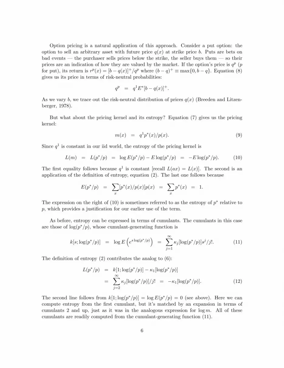
Option pricing is a natural application of this approach. Consider a put option: theoption to sell an arbitrary asset with future price q(x) at strike price b. Puts are bets onbad events — the purchaser sells prices below the strike, the seller buys them — so theirprices are an indication of how they are valued by the market. If the option’s price is qp (pfor put), its return is rp(x) = [b− q(x)]+/qp where (b− q)+ ≡ max{0, b− q}. Equation (8)gives us its price in terms of risk-neutral probabilities:

qp = q1E∗[b− q(x)]+.

As we vary b, we trace out the risk-neutral distribution of prices q(x) (Breeden and Litzen-berger, 1978).

But what about the pricing kernel and its entropy? Equation (7) gives us the pricingkernel:

m(x) = q1p∗(x)/p(x). (9)

Since q1 is constant in our iid world, the entropy of the pricing kernel is

L(m) = L(p∗/p) = log E(p∗/p)−E log(p∗/p) = −E log(p∗/p). (10)

The first equality follows because q1 is constant [recall L(ax) = L(x)]. The second is anapplication of the definition of entropy, equation (2). The last one follows because

E(p∗/p) =∑

x

[p∗(x)/p(x)]p(x) =∑

x

p∗(x) = 1.

The expression on the right of (10) is sometimes referred to as the entropy of p∗ relative top, which provides a justification for our earlier use of the term.

As before, entropy can be expressed in terms of cumulants. The cumulants in this caseare those of log(p∗/p), whose cumulant-generating function is

k[s; log(p∗/p)] = log E(es log(p∗/p)

)=

∞∑

j=1

κj [log(p∗/p)]sj/j!. (11)

The definition of entropy (2) contributes the analog to (6):

L(p∗/p) = k[1; log(p∗/p)]− κ1[log(p∗/p)]

=∞∑

j=2

κj [log(p∗/p)]/j! = −κ1[log(p∗/p)]. (12)

The second line follows from k[1; log(p∗/p)] = log E(p∗/p) = 0 (see above). Here we cancompute entropy from the first cumulant, but it’s matched by an expansion in terms ofcumulants 2 and up, just as it was in the analogous expression for log m. All of thesecumulants are readily computed from the cumulant-generating function (11).

6

To summarize: we can price assets using either a pricing kernel (m) and the true proba-bilities (p) or the price of a one-period bond (q1) and the risk-neutral probabilities (p∗). Thethree objects (m, p∗, p) are interconnected: once we know two (and the price of a one-periodbond), equation (7) gives us the other. That leaves us with three kinds of cumulants cor-responding, respectively, to the true distribution of the random variable x, the risk-neutraldistribution, and the (log) pricing kernel (a function of x). We report all three later in thepaper.

2.3 Evidence

Our goal is to put these tools to work in accounting for broad features of macroeconomicand financial data: consumption growth, asset returns, and option prices. Here’s a quickoverview of US data.

In Table 1 we report familiar evidence on annual consumption growth and equity returnsfor both a long sample (1889-2006) and a shorter one (1986-2006) that corresponds to ourdata on options. The numbers are similar to those reported by Alvarez and Jermann (2005,Tables I-III), Barro (2006, Table IV), and Mehra and Prescott (1985, Table 1). There hasbeen some variation over time in the equity premium (larger in the more recent sample)and consumption growth (less volatile in the recent past), but both may be closer to thelong sample once we include the most recent observations.

In Table 2 we describe prices of options on S&P 500 contracts. Prices are reported asimplied volatilities: values of the volatility parameter of the Black-Scholes-Merton formulathat generates the observed option price. This convention allows a simple comparison to thelognormal case, in which volatility is the same at all strike prices. In the table, we reportaverage implied volatilities of options for a range of strike prices. Observations are annual.They cover options of maturities 1, 3, and 12 months. Since the macroeconomic data areannual, the annual maturity is the most natural in this context, but shorter maturities aremore informative about extreme events. An option of maturity n months, for example,reflects the n-month distribution of index returns. As we increase n, the standardizeddistribution becomes more normal and extreme events are relatively less important. Shorteroptions are also more frequently traded.

Option prices have two features that we examine more closely in Section 5. Similarevidence has been reviewed recently by Bates (2008, Section 1), Drechsler and Yaron (2008,Section 2), and Wu (2006, Section II). The first feature is that implied volatilities are greaterthan sample standard deviations of returns (compare Table 1). Since prices are increasingin volatility, it implies that option prices are high relative to the lognormal Black-Scholes-Merton benchmark. The second is that implied volatilities, hence option prices, are higherfor lower strike prices: the well-known volatility skew. This feature is more evident atshorter maturities, precisely because they are more sensitive to extreme events. It’s alsointriguing from a disaster perspective, because it suggests market participants value adverse

7

events more than is implied by a lognormal model. The question for us whether the extravalue assigned to bad outcomes corresponds to the disasters documented in macroeconomicresearch.

Table 3 is a summary of the evidence: a collection of ballpark numbers that we use astargets for theoretical examples. Thus we consider examples in which the log excess returnon equity has a mean of 0.0440 (4.40%) and a standard deviation of 0.1500. Similarly, logconsumption growth has a mean of 0.0200 and a standard deviation of 0.0350. None of thesenumbers are definitive, but they give us a starting point for considering the quantitativeimplications of theoretical models.

3 Disasters in macroeconomic models and data

Barro (2006), Longstaff and Piazzesi (2004), and Rietz (1988) construct representative-agent exchange economies in which infrequent large declines in consumption improve theirability to generate realistic asset returns: illustrations, in other words, of Zin’s “never adull moment” conjecture. We describe their mechanism with two numerical examples thathighlight the role of high-order cumulants.

The economic environment consists of preferences for a representative agent and astochastic process for consumption growth. Preferences are governed by an additive powerutility function,

E0

∞∑

t=0

βtu(ct),

with u(c) = c1−α/(1 − α) and α ≥ 0. If consumption growth is gt = ct/ct−1, the pricingkernel is

log mt+1 = log β − α log gt+1. (13)

With power utility, the properties of the pricing kernel follow from those of consumptiongrowth. Entropy is

L(m) = L(e−α log g) (14)

and the cumulants of log m are related to those of log g by

κj(log m) = κj(log g)(−α)j/j!, j ≥ 2. (15)

See Section 2.1. If log consumption growth is normal, then so is the log of the pricingkernel. Entropy is then one-half the variance of consumption growth times the risk aversionparameter squared. The impact of high-order cumulants depends on (−α)j/j!. The minussign tells us the negative odd cumulants of log consumption growth generate positive odd

8

cumulants in the log pricing kernel. Negative skewness in consumption growth, for example,generates positive skewness in the pricing kernel and thus helps with the Alvarez-Jermannbound. The magnitudes of high-order cumulants are controlled by αj/j!. Eventually thedenominator grows faster than the numerator, but for moderate values of j, risk aversioncan magnify the contributions of high-order cumulants relative to the contribution of thevariance. Yaron refers to this as a “bazooka”: if α > 1, even moderate high-order cumulantsin log consumption growth can have a large impact on the entropy of the pricing kernel.

We follow Barro (2006) in choosing an iid process for consumption growth so that wecan focus on the role played by its distribution. Let consumption growth be

log gt+1 = wt+1 + zt+1 (16)

with components (wt, zt) that are independent of each other and over time. Since thecomponents are independent, the cumulant-generating function of log g is the sum of thosefor w and z. Similarly, the entropy of the pricing kernel is the sum of the entropy of thecomponents:

L(m) = L(e−αw) + L(e−αz).

Similarly, the cumulants of log m are sums of the cumulants of the components:

κj(log m) = (−α)jκj(w) + (−α)jκj(z), j ≥ 2.

(That’s why they call them cumulants: they “[ac]cumulate.”) We let w ∼ N (µ, σ2), so thatany contribution to high-order cumulants comes from z.

The question is the behavior of z. We consider two examples. In both cases, parametervalues are adapted from Barro (2006), Barro and Ursua (2008), and Barro, Nakamura,Steinsson, and Ursua (2009), who show that sharp downturns are an infrequent but recurringfeature of national consumption and output data.

3.1 Example 1: Bernoulli disasters

The simplest example of a disaster process is a Bernoulli random variable. Suppose thesecond component of consumption growth is

zt ={

0 with probability 1− ωθ with probability ω.

(17)

Here ω and θ < 0 represent the probability and magnitude of a sharp drop in consumptiongrowth (a disaster) relative to its mean. If θ > 0 we have the opposite (a boom). Barro(2006) uses a more complex disaster distribution and Rietz (1988) allows time-dependence,but this is enough to make their point: that an infrequent extreme drop in consumption can

9

have a large impact on asset returns, even when we hold constant the mean and varianceof log consumption growth.

With this structure, we can readily compute entropy and cumulants. The entropy ofthe two components follows from applying its definition (2):

L(e−αw) = (−α)2σ2/2 (18)

L(e−αz) = log(1− ω + ωe−αθ

)+ αωθ. (19)

Both are zero at α = 0 and increase with α. The first expression is the usual “one-half thevariance” of the normal case. The second introduces high-order cumulants; see AppendixA.2.

Two numerical examples, reported as the first two columns of Table 4, illustrate thepotential quantitative significance of the disaster component. Column (1) has normal logconsumption growth (z = 0). Column (2) incorporates a Bernoulli disaster. Parametersin both cases are chosen to match the target values in Table 3. The target values for themean and variance of log g are κ1(log g) = 0.020 and κ2(log g) = 0.0352. Finally, we add thedisaster component. We set ω = 0.01 and θ = −0.3: a one percent chance of a 30 percentfall in (log) consumption relative to its mean. These choices are somewhat arbitrary, butthey’re similar to those of Barro and Rietz. Barro (2006) uses a distribution of disasterswith an overall probability of 0.017 and a distribution whose mean is similar. Rietz usessmaller probabilities and larger disasters.

With these quasi-realistic numbers, we can explore the ability of the model to satisfythe Alvarez-Jermann bound. The observed equity premium implies that the entropy ofthe pricing kernel is at least 0.0440. Without disasters (that is, with ω = 0), the logsof consumption growth and the pricing kernel are normal. The mean and variance of logconsumption growth imply µ = 0.0200 and σ2 = 0.0352. The Alvarez-Jermann boundimplies α2κ2(log g)/2 = α20.0352/2 ≥ 0.0440 or α ≥ 8.47. We can satisfy the Alvarez-Jerman bound for the equity premium, but only with a risk aversion parameter greaterthan 8. There’s a range of opinion about this, but some argue that risk aversion thislarge implies implausible behavior along other dimensions; see, for example, the extensivediscussion in Campanale, Castro, Clementi (2007, Section 4.3) and the references citedthere.

When we add the disaster component, a smaller risk aversion parameter suffices. We dothis holding constant the mean and variance of log consumption growth, so the experimenthas a partial derivative flavor: it measures the impact of high-order cumulants, holdingconstant the mean and variance. We choose µ to equate the mean growth rate to thesample mean: µ + ωθ = 0.0200. Similarly, we choose σ to match the sample variance:

σ2 + ω(1− ω)θ2 = κ2(log g) = 0.0352.

The resulting parameter values are reported in the second column of Table 4. As long asω < 1/2 and θ < 0, the disaster component z introduces negative skewness and positive

10

kurtosis into log consumption growth. Both are evident in first panel of Figure 1, wherewe plot cumulants 2 to 10 for log consumption growth. Each cumulant κj(log g) makes acontribution κj(log g)(−α)j/j! to the entropy of the pricing kernel. The next two panelsof the figure show how the contributions depend on risk aversion. With α = 2, negativeskewness in consumption growth is converted into a positive contribution to entropy, butthe contribution of high-order cumulants overall is small relative to the contribution of thevariance. That changes dramatically when we increase α to 10, where the contribution ofhigh-order cumulants is now greater than that of the variance. This is Yaron’s bazooka inaction: even modest high-order cumulants make significant contributions to entropy if α islarge enough.

Figure 2 gives us another perspective on the same issue: the impact of high-ordercumulants on the entropy of the pricing kernel as a function of the risk aversion parameter α.The horizontal line is the Alvarez-Jerman lower bound, our estimate of the equity premiumin US data. The line labelled “normal” is entropy without the disaster component. Wesee, as we noted earlier, that the entropy of the pricing kernel for the normal case is belowthe lower bound until α is above 8. The line labelled “disasters” incorporates the Bernoullicomponent. The difference between the two lines shows that the overall contribution ofhigh-order cumulants is positive and increases with risk aversion. When α = 2 the extraterms increase entropy by 16%, but when α = 8 the increase is over 100% (Yaron’s bazookaagain).

It’s essential that the extreme events be disasters. If we reverse the sign of θ, the result isthe line labelled “booms” in Figure 2. We see that for every value of α, entropy is below eventhe normal case. The impact of high-order cumulants is apparently negative. Table 5 showsus exactly how this works. With Bernoulli disasters (and α = 10), the entropy of the pricingkernel (0.1614) comes from the variance (0.0613), odd high-order cumulants (0.0621), andeven high-order cumulants (0.0380). When we switch from disasters to booms, the oddcumulants change sign — see equation (15) — reducing overall entropy. Another exampleillustrates the role of the probability and magnitude of the disaster. Suppose we halve θ anddouble ω, with σ adjusting to maintain the variance of consumption growth. Then entropyfalls sharply and the contribution of high-order cumulants almost disappears. In this sense,both the low probability and large magnitude in the example are quantitatively important.

We’ve chosen to focus on the entropy of the pricing kernel, but you get a similar picturein this setting if you look at the equity premium. The short rate r1 = 1/q1 = 1/Em isconstant in our iid environment. We define “levered equity” as a claim to the dividenddt = cλ

t . This isn’t, of course, either equity or levered, but it’s a convenient functionalform that is widely used in the macro-finance literature to connect consumption growth(the foundation for the pricing kernel) to returns on equity (the asset of interest). In theiid case, the log return is a linear function of log consumption growth:

log ret+1 = λ log gt+1 + constant. (20)

See Appendix A.4. The leverage parameter λ allows us to control the variance of the equityreturn separately from the variance of consumption growth and thus to match both. We use

11

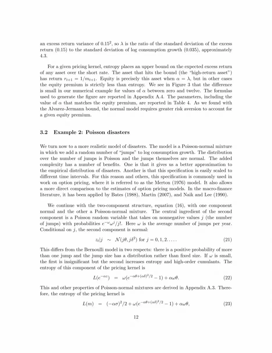
an excess return variance of 0.152, so λ is the ratio of the standard deviation of the excessreturn (0.15) to the standard deviation of log consumption growth (0.035), approximately4.3.

For a given pricing kernel, entropy places an upper bound on the expected excess returnof any asset over the short rate. The asset that hits the bound (the “high-return asset”)has return rt+1 = 1/mt+1. Equity is precisely this asset when α = λ, but in other casesthe equity premium is strictly less than entropy. We see in Figure 3 that the differenceis small in our numerical example for values of α between zero and twelve. The formulasused to generate the figure are reported in Appendix A.4. The parameters, including thevalue of α that matches the equity premium, are reported in Table 4. As we found withthe Alvarez-Jermann bound, the normal model requires greater risk aversion to account fora given equity premium.

3.2 Example 2: Poisson disasters

We turn now to a more realistic model of disasters. The model is a Poisson-normal mixturein which we add a random number of “jumps” to log consumption growth. The distributionover the number of jumps is Poisson and the jumps themselves are normal. The addedcomplexity has a number of benefits. One is that it gives us a better approximation tothe empirical distribution of disasters. Another is that this specification is easily scaled todifferent time intervals. For this reason and others, this specification is commonly used inwork on option pricing, where it is referred to as the Merton (1976) model. It also allowsa more direct comparison to the estimates of option pricing models. In the macro-financeliterature, it has been applied by Bates (1988), Martin (2007), and Naik and Lee (1990).

We continue with the two-component structure, equation (16), with one componentnormal and the other a Poisson-normal mixture. The central ingredient of the secondcomponent is a Poisson random variable that takes on nonnegative values j (the numberof jumps) with probabilities e−ωωj/j!. Here ω is the average number of jumps per year.Conditional on j, the second component is normal:

zt|j ∼ N (jθ, jδ2) for j = 0, 1, 2. . . . . (21)

This differs from the Bernoulli model in two respects: there is a positive probability of morethan one jump and the jump size has a distribution rather than fixed size. If ω is small,the first is insignificant but the second increases entropy and high-order cumulants. Theentropy of this component of the pricing kernel is

L(e−αz) = ω(e−αθ+(αδ)2/2 − 1) + αωθ. (22)

This and other properties of Poisson-normal mixtures are derived in Appendix A.3. There-fore, the entropy of the pricing kernel is

L(m) = (−ασ)2/2 + ω(e−αθ+(αδ)2/2 − 1) + αωθ, (23)

12

the sum of the entropies of the normal and Poisson-normal components.

We illustrate the properties of this example with numbers similar to those used in theBernoulli example. With ω = 0.01, there is probability 0.9900 of no jumps, 0.0099 of onejump, and 0.0001 of more than one jump. With larger values of ω the probability of multiplejumps can be substantial, but in this example it’s miniscule. We set the mean jump sizeθ = −0.3, the same number we used earlier. The only significant change is the dispersionof jumps: we set δ = 0.15. These parameter values are close to those suggested by Barro,Nakamura, Steinsson, and Ursua (2009). Finally, we choose µ and σ to match the samplemean and variance of log consumption growth. In the model, the mean is µ + ωθ and thevariance is σ2 + ω(θ2 + δ2). Given the parameters of the second component, we choose µand σ to match our target values of the mean and variance of log consumption growth. Allof these parameters (and more) are listed in column (3) of Table 4.

This example is qualitatively similar to the previous one, but the dispersion in disastersgenerates greater entropy. The contributions of high-order cumulants are summarized inFigure 4 and Table 5. Figure 5 shows that the model satisfies the Alvarez-Jermann boundat smaller values of α. We match the equity premium with α = 5.38, smaller than the valueof 6.59 needed for the Bernoulli example; see Tables 4 and 5.

4 Risk-neutral probabilities in representative-agent models

As a warmup for our study of options, we consider the risk-neutral probabilities implied bythe examples of the previous section. In general, risk aversion (α > 0) generates risk-neutraldistributions that are shifted left (more pessimistic) relative to true distributions. The formof this shift depends on the distribution.

Our first example has lognormal consumption growth. Suppose log g = w with w ∼N (µ, σ2). Then

p(w) = (2πσ2)−1/2 exp[−(w − µ)2/2σ2].

The pricing kernel is m(w) = β exp(−αw) and the one-period bond price is q1 = Em =β exp[−αµ + (ασ)2/2]. Equation (7) gives us the risk-neutral probabilities:

p∗(w) = p(w)m(w)/q1 = (2πσ2)−1/2 exp[−(w − µ + ασ2)2/2σ2].

Thus risk-neutral probabilities have the same form (normal) with mean µ∗ = µ− ασ2 andstandard deviation σ∗ = σ. The mean shifts the distribution to the left by an amount thatdepends on risk aversion. The log probability ratio is

log [p∗(w)/p(w)] = [(w − µ)2 − (w − µ∗)2]/2σ2 = −(ασ)2/2− α(w − µ),

13

which implies the cumulant-generating function

k[s; log(p∗/p)] = log E(es log p∗/p

)= [(ασ)2/2](−s + s2).

The cumulants are (evidently) zero after the first two. Entropy follows from equation (12),

L(p∗/p) = (ασ)2/2,

which is what we reported in equation (18).

Our second example has Bernoulli consumption growth. Let log g = z, with z equal to0 with probability 1 − ω and θ with probability ω. If we ignore the discount factor β (wejust saw that it drops out when we compute p∗), the pricing kernel is m(z) = e−αz. Theone-period bond price is q1 = 1− ω + ω exp(−αθ). Risk-neutral probabilities are

p∗(z) = p(z)m(z)/q1 ={

(1− ω)/q1 if z = 0ω exp(−αθ)/q1 if z = θ.

Thus p∗ is Bernoulli with probability

ω∗ = ωe−αθ/(1− ω + ωe−αθ)

and magnitude θ∗ = θ. Note that p∗ puts more weight on the bad state than p. Theprobability ratio,

p∗(z)/p(z) ={

1/q1 if z = 0exp(−αθ)/q1 if z = θ,

implies the cumulant-generating function

k[s; log(p∗/p)] = log[(1− ω) + ωe−sαθ

]− s log

[(1− ω) + ωe−αθ

].

Entropy is therefore

L(p∗/p) = (1− ω) log q1 + ω log(q1/e−αθ) = log(1− ω + ωe−αθ) + αωθ,

which is what we saw in equation (19).

In our final example, consumption growth is a Poisson-normal mixture. The Poisson-normal mixture (21) is based on a state space that includes both the number of jumps andthe distribution conditional on the number of jumps: say (j, z). The same logic we used inthe other examples then tells us that the risk-neutral distribution has the same form, withparameters

ω∗ = ω exp(−αθ + (αδ)2/2), θ∗ = θ − αδ2, δ∗ = δ. (24)

Similar expressions are derived by Bates (1988), Martin (2007), and Naik and Lee (1990).Risk aversion (α > 0) places more weight on bad outcomes in two ways: they occur morefrequently (ω∗ > ω if θ < 0) and are on average worse (θ∗ < θ). Entropy is the same asreported in (22).

We won’t bother with multi-component models, but they follow similar logic. If logconsumption growth is the sum of independent components, then entropy is the sum of theentropies of the components, as in equation (23).

14

5 Disasters in option models and data

In the macro-finance literature, pricing kernels are typically constructed as in Section 3:we apply a preference ordering (power utility in our case) to an estimated process forconsumption growth (lognormal or otherwise). In the option-pricing literature, pricingkernels are constructed from asset prices alone: true probabilities are estimated from timeseries data on prices or returns, risk-neutral probabilities are estimated from cross-sectiondata, and the pricing kernel is computed from the ratio. The approaches are complementary;they generate pricing kernels from different data. The question is whether they lead tosimilar conclusions. Do options on US equity indexes imply the same kinds of extremeevents that Barro and Rietz suggested? Equity index options are a particularly informativeclass of assets for this purpose, because they tell us not only the market price of equityreturns overall, but the prices of specific outcomes, including outcomes well outside thenorm.

5.1 The Merton model

We look at option prices through the lens of the Merton model, a functional form thathas been widely used in the empirical literature on option prices. The starting point is astochastic process for asset prices or returns. Since we’re interested in the return on equity,we let

log ret+1 − log r1 = wt+1 + zt+1. (25)

We use the return, rather than the price, because it fits neatly into our iid framework, butthe logic is the same either way. As before, the components (wt, zt) are independent of eachother and over time. Market pricing of risk is built into differences between the true andrisk-neutral distributions of the two components. We give the distributions the same form,but allow them to have different parameters. The first component, w, has true distributionN (µ, σ2) and risk-neutral distribution N (µ∗, σ2). By convention, σ is the same in bothdistributions, a byproduct of its continuous-time origins. The second component, z, is aPoisson-normal mixture. The true distribution has jump intensity ω and the jumps areN (θ, δ2). The risk-neutral distribution has the same form with parameters (ω∗, θ∗, δ∗).

Related work supports a return process with these features. Ait-Sahalia, Wang, andYared (2001) report a discrepancy between the risk-neutral density of S&P 500 index returnsimplied by the cross-section of options and the time series of the underlying asset returns,but conclude that the discrepancy can be resolved by introducing a jump component. Onemight go on to argue that two jumps are needed: one for macroeconomic disasters andanother for more frequent but less extreme financial crashes. However, Bates (2009) studiesthe US stock market over the period 1926-2006 and shows that a second jump componentplays no role in accounting for macroeconomic events like the Depression.

15

Given this structure, the pricing kernel follows from equation (9). Its entropy is

L(m) = L(p∗/p)

=12

(µ− µ∗

σ

)2

+ (ω∗ − ω) + ω

[log

ω

ω∗− log

δ

δ∗+

(θ − θ∗)2 + (δ2 − δ∗2)2δ∗2

]. (26)

The source of this expression and the corresponding cumulant-generating function are re-ported in Appendix A.5.

5.2 Parameter values

We use parameter values from Broadie, Chernov, and Johannes (2007), who summarize andextend the existing literature on equity index options. The parameters of the true distribu-tion are estimated from the time series of excess returns on equity. We use the parametersof the Poisson-normal mixture — namely (ω, θ, δ) — reported in Broadie, Chernov, andJohannes (2007, Table I, the line labelled SVJ EJP). These estimates also include stochas-tic volatility, which we ignore because it conflicts with our iid structure. The estimatedjump intensity ω is 1.512, which implies much more frequent jumps than we used in ourconsumption-based model. With this value, the probability of 0 jumps per year is 0.220,1 jump per year 0.333, 2 jumps 0.25, 3 jumps 0.13, 4 jumps 0.05, and 7 or more jumpsabout 0.001. Properties related to extreme events can be difficult to estimate precisely, aswe noted in the introduction. The issue is their frequency. If they occur (say) once everyhundred years, a long dataset is a necessity. If they’re more frequent, as estimates based onUS stock returns imply, we can get precise estimates from a finer time interval, even overshorter samples. Given parameters for the Poisson-normal component, µ and σ are chosento match the mean and variance of excess returns to their target values. In the model, themean excess return (the equity premium) is µ + ωθ, which determines µ. The variance isσ2 + ω(θ2 + δ2), which determines σ. The results are reported in Table 4.

The risk-neutral parameters for the Poisson-normal mixture are estimated from thecross section of option prices: specifically, prices of options on the S&P 500 over the period1987-2003. The depth of the market varies both over time and by the range of strike prices,but there are enough options to allow reasonably precise estimates of the parameters. Thenumbers we report in Table 4 are from Broadie, Chernov, and Johannes (2007, Table IV,line 5). In practice, option prices identify only the product ω∗θ∗, so they set ω∗ = ω andchoose θ∗ and δ∗ to match the level and shape of the implied volatility smile. Finally, µ∗ isset to satisfy (8), which implies µ∗ + σ2/2 + ω∗[exp(θ∗ + δ∗2/2)− 1] = 0.

Figure 6 shows how θ∗ and δ∗ are identified from the cross section of 3-month optionprices. We express prices as implied volatilities and graph them against “moneyness,” withhigher strike prices to the right. In the data, we measure moneyness as the log of the ratio ofthe strike price to the spot price. In the figure, the solid line illustrates the slope and shapeof the implied volatility smile in the model. Since the model fits extremely well, we can take

16

this as a reasonable representation of the data. The downward slope and convex shape areboth evidence of departures from lognormality. They also illustrate how the parameters areidentified. Consider three values of θ∗: −0.0259 (= θ), +0.0259, and the estimated value−0.0482. We plot volatility smiles for all three values with δ∗ = δ. Evidently θ∗ controlsthe slope. When it’s positive, the smile slopes upward, and when it’s a smaller negativevalue than our estimate the smile is flatter. All of these smiles lie below the estimated one.The value of δ∗ affects the level and curvature of the smile. This is evident from the smilefor δ∗ = δ, a substantially smaller value. The combination produces an implied volatilitysmile that closely approximates the slope and curvature we see in the data.

5.3 Pricing kernels implied by options

In Table 4 we report the parameters of the option model and some of their implications, andin Table 5 we report the entropy of the pricing kernel and its components. Three featuresof the option model deserve emphasis.

The first and most important feature of the option model is that odd high-order cumu-lants make a substantial contribution to entropy. In this respect, the option model agreeswith the macroeconomic models of disasters we examined earlier. The contribution of oddhigh-order cumulants is larger than we saw in macroeconomic models, but smaller as afraction of entropy.

The second feature is that disasters are more moderate in our option model [column (4)]than in a similar model based on consumption data [column (3)]. The units are different(consumption growth v. returns), so it’s not a direct comparision unless the two are linked— as they are in our equation (20). With this caveat in mind, note that standardizedmeasures of skewness and kurtosis are substantially smaller in the option model than in themodel based on consumption evidence. This is true whether we look at the true distribution,the risk-neutral distribution, or the distribution of the pricing kernel. The same holds fortail probabilities: probabilities of extreme negative realizations of consumption growth orthe return on equity. Outcomes more than 3 and 5 standard deviations to the left of themean are more likely in the model based on consumption evidence [column (3) of the table]than in the model based on option prices [column (4)].

The third feature is that entropy is significantly higher. While the macro models hadentropy less than 0.1, the option model implies entropy of almost 0.8. This reflects, inlarge part, the high price of options. The prices are high in the sense that selling themgenerates high average returns; see, for example, Broadie, Chernov, and Johannes (2009).These high average returns imply high entropy via the Alvarez-Jermann bound. Evidentlya bound based on the equity premium is too loose: other investment strategies generatehigher average excess returns and therefore imply higher entropy.

We look more closely at the differences between consumption- and option-based modelsin the next section.

17

6 Comparing consumption- and option-based models

We’ve seen that disasters implied by options are considerably different from those apparentin consumption data. We explore the difference further in this section, looking at optionprices implied by consumption growth, consumption growth implied by option prices, andrisk aversion implicit in options data. These comparisons highlight the relations betweentrue and risk-neutral probabilities implied by consumption- and option-based models, re-spectively.

Consider first the option prices implied by our consumption-based model. In essence,we are taking the true distribution of consumption growth implied by consumption data,computing the risk-neutral distribution by applying power utility, and using the risk-neutraldistribution to compute option prices. The only missing link is the connection between con-sumption growth (the natural random variable for consumption-based models) and equityreturns (the natural variable for option-based models). In our environment, the two areconnected by (20): equity returns are a log-linear function of consumption growth withslope λ. To convert the consumption growth process to a return process, we multiply θ andδ by λ and keep the jump intensity ω the same. Risk-neutral parameters then follow from(24).

Implied volatility smiles for the consumption-based model are pictured in Figure 7 alongwith those for the estimated Merton model. Similar consumption-based volatility smiles arereported by Benzoni, Collin-Dufresne, and Goldstein (2005) and Du (2008). What’s new isthe explicit comparison to an estimated option pricing model. We report two smiles in eachcase, corresponding to 3-month and 12-month options. The two models are clearly different.The consumption-based model has a steeper smile, greater curvature, and lower at-the-money volatility. The reason, again, is that it has both higher risk-neutral probabilities oflarge disasters (the left side of the figure) and lower probabilities of less extreme outcomes(the middle and right of the figure). Stated simply: the difference in extreme outcomesbetween models based on macroeconomic and options data results in significantly differentoption prices. This is evident, for example, in the large difference in risk-neutral skewnessand kurtosis reported in columns (3) and (4) of Table 4.

Now consider the reverse: the consumption growth process implied by the risk-neutraldistribution of equity returns indicated by option prices. Here we are taking the risk-neutraldistribution and computing the true distribution using (again) power utility. This procedureplaces more structure on the problem than we used in the option model — namely, powerutility. Given this structure, we can infer the true distribution without relying on the limitedtime series evidence available for estimating it directly from consumption. Again, we needto rescale the parameters, dividing θ∗ and δ∗ by λ. Given these values, we compute theparameters of the true distribution using (24). Finally, we set σ to match our target for thestandard deviation of log consumption growth and α to match the equity premium. Theresults are reported in column (5) of Table 4.

18

The consumption process derived this way from option prices generates disasters inthe sense that large declines in consumption growth are substantially more likely than ina lognormal model. They are, however, more moderate than we see in macroeconomicdata. This is evident in the standardized measures of skewness and excess kurtosis. It’salso evident in the probabilities of tail events. The probability of (at least) 3 standarddeviation declines is similar in the two models. Roughly speaking, there’s just under a 1percent chance of a drop in consumption similar to the US in the Depression. However, 5standard deviation declines are much more likely in the consumption-based model [column(3)] than in the option-based model [column (5)]. The risk aversion parameter must belarger to compensate for the more modest disasters. We see this directly in Table 5, wherethe contribution of high-order cumulants is much smaller than in the Poisson model basedon consumption evidence.

Both of these comparisons use power utility to connect true and risk-neutral parameters,yet the parameter values of the option model are inconsistent with power utility. Oneexample is the difference between δ and δ∗, which is zero with power utility [equation 24)].Nevertheless, we can derive something like risk aversion from our option model. Note thatin (13), risk aversion is implicit in the relation between the pricing kernel and consumptiongrowth:

α = −∂ log m

∂ log g.

In the option model, the analogous expression is

RA = −∂ log(p∗/p)∂ log re

· ∂ log re

∂ log g.

See Leland (1980). In our setting, the second term is λ, so the action is in the first term.

Risk aversion defined this way need not have much to do with the risk aversion ofindividual agents, but it’s a useful way of describing how the market prices risk. Optionprices imply that RA depends, in general, on the state; see Appendix A.6. In our case, it’slarger for negative returns than for positive ones, with risk aversion of 14 for returns of –10%and 3.5 for returns of +10%. Related work has generated a wide range of patterns, butthey all find that risk aversion varies with the state. See, for example, Ait-Sahalia and Lo(2000), Jackwerth (2000), Rosenberg and Engle (2002), and Ziegler (2007). What we findinteresting is the possibility that risk premiums on assets might reflect not only disasters inoutcomes but pricing of disasters that gives them greater weight than power utility.

7 Summary and extensions

We have described, in a relatively simple theoretical setting, how option prices can be usedto infer the probabilities of disasters, including the infrequent sharp declines in consumption

19

growth documented in macroeconomic data by Barro (2006) and others. Options on theS&P 500 index value bad outcomes more than good ones, and in this sense are similarto the macroeconomic evidence. The disasters implied by option prices are, however, moremodest. The analysis that leads to these conclusions leans heavily on three supports: powerutility over aggregate consumption, iid consumption growth, and a close connection betweenaggregate dividends and consumption. Each deserves a closer look.

Perhaps the most interesting extension of the theory is to consider going beyond powerutility or even the representative agent framework. Power utility is the workhorse of macroe-conomics and finance, but our option model suggests greater aversion to bad outcomes thangood ones. If this turns out to be a robust feature of the evidence, it’s worth thinking aboutwhere it comes from. One possibility is explore alternative preferences, including skewnessaversion (Harvey and Siddique, 2000), Chew-Dekel risk preferences (reviewed by Backus,Routledge, and Zin, 2004), state-dependent preferences (Chabi-Yo, Garcia, and Renault,2008), ambiguity (applied to options by Drechsler, 2008, and Liu, Pan, and Wang, 2005),learning (Shaliastovich, 2008), and habits (Du, 2008). Another promising avenue is het-erogeneity across agents. Certainly there is clear evidence of imperfect risk-sharing acrossindividuals and good reason to suspect that this might affect asset prices. Alvarez, Atke-son, and Kehoe (2009), Bates (2008), Chan and Kogan (2002), Guvenen (2009), and Lustigand Van Nieuwerburgh (2005) are notable examples. The question for us is whether theseextensions provide a persuasive explanation for prices of equity index options.

Another interesting extension is time-dependence. There’s overwhelming evidence thatshort-term interest rates, implied volatilities, and expected returns on a variety of assetschange through time. None of this is consistent with our iid setting. The question iswhether time-dependence is quantitatively important in assessing the role of extreme events,particularly their impact on the entropy of the pricing kernel. It’s possible the role is small.We know, for example, that the variance of the conditional mean of the pricing kernel is muchless than the mean conditional variance; see Cochrane and Hansen (1992, Section 2.7). Asimilar relation holds for entropy. Nevertheless, recent work by Drechsler and Yaron (2008)and Wachter (2008) suggest that time-variation in the distribution over extreme events canbe quantitatively important for asset pricing.

The third extension is to loosen the link between dividends and consumption. We’vefollowed a long tradition in tying dividends to consumption. The tradition is largely amatter of convenience, because it’s simpler to have one random variable rather than two.Our focus on the pricing kernel and its entropy reinforces this message, since neither dependson the dividend process. Nevertheless, the work of Bansal and Yaron (2007), Gabaix (2009),and Longstaff and Piazzesi (2004) suggests that this extension has promise in accountingfor the behavior of equity prices and returns.

20

A Appendix

A.1 The Alvarez-Jermann bound

The Alvarez-Jermann bound (3) is a byproduct of Proposition 2 in Alvarez and Jermann(2005). The proof goes like this:

• Bound on mean log return. Since log is a concave function, Jensen’s inequality andthe unconditional version of the pricing relation (1) imply that for any positive returnr,

E log m + E log r ≤ log(1) = 0,

with equality if and only if mr = 1. Therefore no asset has higher expected (log)return than the inverse of the pricing kernel:

E log r ≤ −E log m. (27)

In finance, the asset with this return is sometimes called the “growth optimal portfo-lio.” We call it the “high-return asset.”

• Short rate. A one-period (risk-free) bond has price q1t = Etmt+1, so its return is

r1t+1 = 1/Etmt+1.

• Entropy of the one-period bond price. With the bound in mind, our next step is toexpress E log r1 in terms of unconditional moments. The entropy of the one-periodbond price does the trick:

L(q1) = log Eq1 − E log q1 = log Em + E log r1. (28)

• Alvarez-Jermann bound. (27) and (28) imply

L(m) ≥ E(log rj − log r1

)+ L(q1).

Inequality (3) follows from L(q1) ≥ 0 (entropy is nonnegative). In practice, L(q1) issmall; in the iid case, it’s zero.

We find the loglinear perspective of the Alvarez-Jerman bound convenient, but the familiarHansen-Jagannathan bound also depends (implicitly) on high-order cumulants of logm.The bound is

Var(m)1/2/Em ≥ E(rj − r1

)/Var(rj − r1)1/2,

21

where the expression on the right is the Sharpe ratio. The bound depends on

Em = E(elog m

)= ek(1)

Var(m) = E(m2)− (Em)2 = ek(2) − e2k(1),

where k(s) is the cumulant generating function of log m. Because k(s) depends on thehigh-order cumulants of log m, the bound does, too. The squared Sharpe ratio is boundedabove by

Var(m)/E(m)2 = ek(2)−2k(1) − 1.

If the cumulants are small (true for a small enough time interval), this is approximatelyk(2)− 2k(1). Expressed in similar form, entropy is k(1)− k′(0).

A.2 Entropy and cumulants of Bernoulli random variables

We derive the entropy and cumulants of a Bernoulli random variable, as in Section 3. Let ztake on the values 0 and 1 with probabilities 1−ω and ω. Entropy follows from its definition(2):

L(ez) = log(1− ω + ωe1

)− ω.

Cumulants can be used to quantify the contribution of specific terms. The cumulant-generating function for w is

k(s) = log Eesz = log(1− ω + ωes).

Cumulants are derivatives evaluated at s = 0: κj = k(j)(0). The derivatives

k(1)(s) = e−k(s)ωes

k(2)(s) = k(1)(s)[1− k(1)(s)]k(3)(s) = k(2)(s)[1− 2k(1)(s)]k(4)(s) = k(3)(s)[1− 2k(1)(s)]− 2[k(2)(s)]2

k(5)(s) = k(4)(s)[1− 2k(1)(s)]− 6k(2)(s)k(3)(s)

imply the cumulants

κ1 = ω

κ2 = κ1(1− κ1) = ω(1− ω)κ3 = κ1(1− κ1)(1− 2κ1) = ω(1− ω)(1− 2ω)κ4 = κ3(1− 2κ1)− 2(κ2)2 = ω(1− ω)(6ω2 − 6ω + 1)κ5 = κ4(1− 2κ1)− 6κ2κ3 = ω(1− ω)(1− 2ω)(12ω2 − 12ω + 1).

It’s evident that odd moments come from ω 6= 1/2. The example in Section 3 is the samerandom variable multiplied by θ.

22

A.3 Entropy and cumulants of Poisson-normal mixtures

We’ll look at a Poisson-normal mixture shortly, but it’s useful to start with a Poissonrandom variable z that equals j with probability e−ωωj/j! for j = 0, 1, 2, . . .. Recall thatthe power series representation of the exponential function is

eω =∞∑

j=0

ωj/j!,

which ensures that the probabilities sum to one. The moment-generating function is

h(s) =∞∑

j=0

e−ωωj/j!esj =∞∑

j=0

e−ω(ωes)j/j! = exp[ω(es − 1)].

The cumulant-generating function is therefore

k(s) = log h(s) = ω(es − 1).

Cumulants follow directly.

The Poisson-normal mixture has a similar structure. Conditional on j, z is normal withmean jθ and variance jδ2. The conditional moment-generating function is exp[(sθ +s2δ2/2)j]. The mgf for the mixture is the probability-weighted average,

h(s) =∞∑

j=0

e−ωωj/j! exp[(sθ + s2δ2/2)j] = exp(ω(esθ+(sδ)2/2 − 1)

),

which implies the cgf

k(s) = ω(esθ+(sδ)2/2 − 1

).

The same approach can be used for jumps with any distribution. If we set θ = 1 and δ = 0,we get the cgf of the original Poisson.

We find cumulants the usual way, taking derivatives of k. The first five are

κ1 = ωθ

κ2 = ω(θ2 + δ2)κ3 = ωθ(θ2 + 3δ2)κ4 = ω(θ4 + 6θ2δ2 + 3δ4)κ5 = ωθ(θ4 + 10θ2δ2 + 15δ4).

Here you can see that the sign of the odd moments is governed by the sign of θ. Negativeodd cumulants evidently require θ < 0.

23

A.4 Equity premium and cumulants with power utility

Most of our analysis is loglinear, which allows us to express asset prices and returns asfunctions of cumulant-generating functions of (say) the log of consumption growth. Thenotation is a little obscure, but it’s wonderfully compact. The idea and many of the resultsfollow Martin (2008).

Let’s start with the short rate. A one-period risk-free bond sells at price q1t = Etmt+1 and

has return r1t+1 = 1/q1

t = 1/Etmt+1. In the iid case, the short rate is constant and equals

log r1 = − log E(m)

= − log β − log E(e−α log g

)= − log β − k(−α; log g).

The second equality is based on the definition of the pricing kernel, equation (13). The lastone follows from the definition of the cumulant-generating function k, equation (4).

We now turn to equity, defined as a claim to a dividend process dt = cλt . If the price-dividend

ratio on this claim is qe, the return is

ret+1 = gλ

t+1(1 + qet+1)/qe

t .

In the iid case, qe is constant. The pricing relation (1) and our power utility pricing kernel(13) then imply

qe/(1 + qe) = E(βgλ−α

)= βE

(e(λ−α) log g

).

Thus we have, in compact notation,

log [qe/(1 + qe)] = log β + k(λ− α; log g)log re

t+1 = λ log gt+1 − log β − k(λ− α; log g)log r1

t+1 = − log β − k(−α; log g)log re

t+1 − log r1t+1 = λ log gt+1 + k(−α; log g)− k(λ− α; log g).

The equity premium is therefore

E(log re

t+1 − log r1t+1

)= λκ1(log g) + k(−α; log g)− k(λ− α; log g)

= L(e−α log g)− L(e(λ−α) log g)

=∞∑

j=2

κj(log g)[(−α)j − (λ− α)j ]/j!.

The second line follows because the first-order cumulants cancel. The third is the usualcumulant expansion of entropy. They tell us that the equity premium is the entropy ofthe pricing kernel minus a penalty (entropy must be positive). It hits its maximum whenλ = α, in which case equity is the high return asset.

24

A similar approach reveals the connection between true and risk-neutral cumulants of logconsumption growth log g = w (w because it’s easier to type). The cumulant generatingfunction for the true distribution is

k(s) = log E (esw) .

The pricing kernel is m(w) = βe−αw, which implies q1 = βk(−α). Risk-neutral probabilitiesare p∗(w) = p(w)m(w)/q1 = p(w)e−αw/k(−α) . The cumulant generating function istherefore

k∗(s) = k(s− α)− k(−α).

This is a standard math result. We find its cumulants by differentiating:

κ∗n =∞∑

j=0

κn+j(−α)j/j!.

Note, for example, that risk-neutral cumulants depend on higher-order true cumulants.Positive excess kurtosis, for example, reduces risk-neutral skewness.

A.5 Cumulant-generating functions based on risk-neutral probabilities

We derive the salient features of models in which the true and risk-neutral distributions arePoisson mixtures of normals with different parameters.

We start with a normal example that serves as a component of the Poisson mixture. Let thelog return follow (25), where z = 0 and w has true distribution of N (µ, σ2) and risk-neutraldistribution N (µ∗, σ∗2). The density functions are

p(w) = (2πσ2)−1/2 exp[−(w − µ)2/2σ2]p∗(w) = (2πσ∗2)−1/2 exp[−(w − µ∗)2/2σ∗2].

This differs from our earlier examples in allowing the variance to differ between the twodistributions. In continuous time, σ∗ = σ is needed to assure absolute continuity of the trueand risk-neutral probability measures with respect to each other. In discrete time, there isno such requirement; see, for example, Buhlmann, Delbaen, Elbrechts, and Shiryaev (1996).The risk-neutral pricing relation (8) implies µ∗ + σ∗2/2 = 0.

We can derive all of the relevant properties from these inputs. The log probability ratio is

log[p∗(w)/p(w)] = (1/2) log ϕ + [(w − µ)2 − ϕ(w − µ∗)2]/2σ2,

25

where ϕ = σ2/σ∗2 > 0. The moment-generating function of the log probability ratio is

h(s; log p∗/p) = E(es log p∗/p

)

=∫ ∞

−∞p∗(w)sp(w)1−sdw

= (2πσ2)−1/2ϕs/2

∫ ∞

−∞exp{−[(1− s)(w − µ)2 + sϕ2(w − µ∗)2]/2σ2}dw

= ϕs/2[1− s(1− ϕ)]−1/2 exp(

s(s− 1)(µ∗ − µ)2

2σ∗2[1− s(1− ϕ)]

)

for 1 − s(1 − ϕ) > 0 (automatically satisfied if s = 0 or s = 1). The last line follows fromcompleting the square. Thus the cumulant-generating function is

k(s; log p∗/p) = (s/2) log ϕ− (1/2) log[1− s(1− ϕ)] +(

s(s− 1)(µ∗ − µ)2

2σ∗2[1− s(1− ϕ)]

).

Entropy is minus the first derivative evaluated at zero:

− κ1(log p∗/p) = (1/2)[log ϕ + 1− ϕ] + (µ− µ∗)2/2σ∗2. (29)

If ϕ = 1 (σ∗ = σ), we have

k(s; log p∗/p) = s(s− 1)(µ∗ − µ)2/2σ2,

and the only nonzero cumulants are the first two. Otherwise, high-order cumulants aregenerally nonzero.

Now let’s ignore the normal component and focus on z. Both the true and risk-neutraldistributions have Poisson arrivals and normal jumps, but the parameters differ. Conditionalon a number of jumps j, the density functions are

p(z|j) = e−ωωj/j! · (2πjδ2)−1/2 exp[−(zj − jθ)2/(2jδ2)]

p∗(z|j) = e−ω∗ω∗j/j! · (2πjδ∗2)−1/2 exp[−(zj − jθ∗)2/(2jδ∗2)].

The moment generating function for log p∗/p is

h(s; log p∗/p) =∞∑

j=0

e−ωωj/j![es(ω−ω∗)+js log(ω∗/ω)h(s; z)j

].

Using (29) we have

h(s; z) = ϕs/2[1− s(1− ϕ)]−1/2 exp(

s(s− 1)(θ∗ − θ)2

2δ∗2[1− s(1− ϕ)]

),

where ϕ = δ2/δ∗2. Therefore the cumulant-generating function is

k(s; log p∗/p) = s(ω − ω∗)

+ ω

[(ω∗/ω)sϕs/2[1− s(1− ϕ)]−1/2 exp

(s(s− 1)(θ∗ − θ)2

2δ∗2[1− s(1− ϕ)]

)− 1

].

26

Entropy is minus the first derivative evaluated at zero:

− κ1(log p∗/p) (30)= (ω∗ − ω) + ω[log(ω/ω∗)− 1/2 · log ϕ + 1/2 · (ϕ− 1)] + ω(θ − θ∗)2/2δ∗2.

Because the normal and Poisson mixture components are independent, their cumulant-generating functions are additive. Therefore, the entropy for the full model is the sum ofthe entropy of the normal case [equation (29) with ϕ = 1] and the entropy of the Poissonmixture of normals [equation (30)].

A.6 Risk aversion implied by the Merton model

We compute risk aversion as:

RA = −∂ log(p∗/p)∂ log g

= −∂ log(p∗/p)∂ log re

· ∂ log re

∂ log g

=(

1p· ∂p

∂ log re− 1

p∗· ∂p∗

∂ log re

)· λ.

Given the normal distribution of jumps, the density conditional on the number of jumps jis

p(log re, j) = e−ωωj/j! · [2π(σ2 + jδ2)]−1/2 exp{−(log re − µ− jθ)2/[2(σ2 + jδ2)]

}.

The (marginal) density for log-returns is

p(log re) =∞∑

j=0

p(log re|j)p(j) =∞∑

j=0

p(log re, j).

Therefore,

∂p(log re)∂ log re

= −∞∑

j=0

p(log re, j) · (log re − µ− jθ)/(σ2 + jδ2).

A similar expression holds for the risk-neutral distribution.

As a result, implied risk aversion is

RA/λ =1∑∞

j=0 p∗(log re, j)

∞∑

j=0

p∗(log re, j) · (log re − µ∗ − jθ∗)/(σ2 + jδ∗2)

− 1∑∞j=0 p(log re, j)

∞∑

j=0

p(log re, j) · (log re − µ− jθ)/(σ2 + jδ2). (31)

Note that RA is a function of the state through log re.

27

References

Ait-Sahalia, Yacine, and Andrew W. Lo, 2000, “Nonparametric risk management and im-plied risk aversion,” Journal of Econometrics 94, 9-51.

Ait-Sahalia, Yacine, Yubo Wang, and Francis Yared, 2001, “Do option markets correctlyprice the probabilities of movement of the underlying price?,” Journal of Economet-rics 102, 67-110.

Alvarez, Fernando, Andrew Atkeson, and Patrick J. Kehoe, 2009, “Time-varying risk, in-terest rates, and exchange rates in general equilibrium,” Review of Economic Studies76, 851-878.

Alvarez, Fernando, and Urban Jermann, 2005, “Using asset prices to measure the persistenceof the marginal utility of wealth,” Econometrica 73, 1977-2016.

Backus, David K., Bryan R. Routledge, and Stanley E. Zin, 2004, “Exotic preferences formacroeconomists,” NBER Macroeconomics Annual 19, 319-390.

Bansal, Ravi, and Amir Yaron, 2007, “The asset pricing-macro nexus and return-cash flowpredictability,” manuscript, June.

Barro, Robert J., 2006, “Rare disasters and asset markets in the twentieth century,” Quar-terly Journal of Economics 121, 823-867.

Barro, Robert J., Emi Nakamura, Jon Steinsson, and Jose F. Ursua, 2009, “Crises andrecoveries in an empirical model of consumption disasters,” manuscript, June.

Barro, Robert J., and Jose F. Ursua, 2008, “Macroeconomic crises since 1870,” BrookingsPapers on Economic Activity , 255-335.

Bates, David, 1988, “Pricing options under jump-diffusion processes,” manuscript.

Bates, David, 2008, “The market for crash risk,” Journal of Economic Dynamics and Con-trol 32, 2291-2231.

Bates, David, 2009, “US stock market crash risk, 1926-2006,” manuscript, March.

Benzoni, Luca, Pierre Collin-Dufresne, and Robert S. Goldstein, 2005, “Can standard pref-erences explain the prices of out-of-the-money S&P 500 put options?,” manuscript,September.

Breeden, Douglas T. and Robert H. Litzenberger, 1978, “Prices of state-contingent claimsimplicit in option prices,” Journal of Business 51, 621-651.

Broadie, Mark, Mikhail Chernov, and Michael Johannes, 2007, “Model specification andrisk premia: evidence from futures options,” Journal of Finance 62, 1453-1490.

Broadie, Mark, Mikhail Chernov, and Michael Johannes, 2009, “Understanding index optionreturns,” Review of Financial Studies, in press.

Buhlmann, Hans, Freddy Delbaen, Paul Embrechts, and Albert Shiryaev, 1996, “No-

28

arbitrage, change of measure, and conditional Esscher transforms,” CWI Quarterly9, 291-317.

Campanale, Claudio, Rui Castro, Gian Luca Clementi, 2007, “Asset pricing in a productioneconomy with Chew-Dekel preferences,” manuscript, April.

Chan, Yeung Lewis, and Leonid Kogan, 2002, “Catching up with the Joneses: heterogeneouspreferences and the dynamics of asset prices,” Journal of Political Economy 110,1255-1285.

Chabi-Yo, Fousseni, Rene Garcia, and Eric Renault, 2008, “State-dependence can explainthe risk aversion puzzle,” Review of Financial Studies 21, 973-1011.

Cochrane, John C., and Lars Peter Hansen, 1992, “Asset pricing explorations for macroe-conomics,” NBER Macroeconomics Annual 7, 115-165.

Drechsler, Itamar, 2008, “Uncertainty, time-varying fear, and asset prices,” manuscript,December.

Drechsler, Itamar, and Amir Yaron, 2008, “What’s vol got to do with it?” manuscript,December.

Du, Du, 2008, “How bad will the potential economic disasters be? Evidences from S&P500 index options data,” manuscript, June.

Gabaix, Xavier, 2009, “Variable rare disasters: an exactly solved framework for ten puzzlesin macro-finance,” manuscript, March.

Guvenen, Fatih, 2009, “A parsimonious macroeconomic model for asset pricing,” Econo-metrica, forthcoming.

Hansen, Lars Peter, and Ravi Jagannathn, 1991, “Implications of security market data formodels of dynamic economies,” Journal of Political Economy 99, 225-262.

Harvey, Campbell R., and Akhtar Siddique, 2000, “Conditional skewness in asset pricingtests,” Journal of Finance 55, 1263-1295.

Jackwerth, Jens Carsten, 2000, “Recovering risk aversion from option prices and realizedreturns,” Review of Financial Studies 13, 433-451.

Leland, Hayne E., 1980, “Who should buy portfolio insurance?,” Journal of Finance 35,581-594.

Liu, Jun, Jun Pan, and Tan Wang, 2005, “An equilibrium model of rare-event premia andits implication for option smirks,” Review of Financial Studies 18, 131-164.

Longstaff, Francis A., and Monika Piazzesi, 2004, “Corporate earnings and the equity pre-mium,” Journal of Financial Economics 74, 401-421.

Lustig, Hanno N., and Stijn G. Van Nieuwerburgh, 2005, “Housing collateral, consumptioninsurance, and risk premia: an empirical perspective, ” Journal of Finance 60, 1167-1219.

29

Martin, Ian, 2007, “Disasters and asset pricing: evidence from option markets,” manuscript,February.

Martin, Ian, 2008, “Consumption-based asset pricing with higher cumulants,” manuscript,March.

Mehra, Rajnish, and Edward C. Prescott, 1985, “The equity premium: a puzzle,” Journalof Monetary Economics 15, 145-161.

Merton, Robert C., 1976, “Option pricing when underlying stock returns are discontinuous,”Journal of Financial Economics 3, 125-144.

Naik, Vasanttilak, and Moon Lee, 1990, “General equilibrium pricing of options on themarket portfolio with discontinuous returns,” Review of Financial Studies 3, 493-521.

Rietz, Thomas A., 1988, “The equity risk premium: a solution,” Journal of MonetaryEconomics 22, 117-131.

Rosenberg, Joshua V., and Robert F. Engle, 2002, “Empirical pricing kernels,” Journal ofFinancial Economics 64, 341-372.

Shaliastovich, Ivan, 2008, “Learning, confidence and option prices,” manuscript.

Shiller, Robert, 2007, “Long term stock, bond, interest rate and consumption data,” spread-sheet posted on his web site.

Wachter, Jessica, 2009, “Can time-varying risk of rare disasters explain aggregate stockmarket volatility?,” manuscript, March.

Wu, Liuren, 2006, “Dampened power law: reconciling the tail behavior of financial securityreturns,” Journal of Business 79, 1445-1474.

Ziegler, Alexandre, 2007, “Why does implied risk aversion smile?,” Review of FinancialStudies 20, 859-904.

Zin, Stanley, 2002, “Are behavioral models of asset-pricing structural?,” Journal of Mone-tary Economics 49, 215-228.

30

Table 1Properties of consumption growth and asset returns

Variable Mean Std Dev Skew Kurt Auto

Consumption and returns, 1889-2006Consumption growth 0.0200 0.0353 –0.35 1.10 –0.07Return on one-year bond 0.0182 0.0573 0.03 2.29 0.35Return on equity 0.0622 0.1737 –0.50 0.18 0.04Excess return on equity 0.0440 0.1748 –0.60 0.71 0.07Consumption and returns, 1986-2006Consumption growth 0.0186 0.0131 –0.59 –0.20 0.48Return on one-year bond 0.0221 0.0190 –0.45 –0.68 0.41Return on equity 0.0845 0.1470 –0.58 –0.52 0.15Excess return on equity 0.0625 0.1397 –0.67 –0.58 0.17

Notes. Entries are sample moments. Mean is the sample mean, Std Dev is the standarddeviation, Skew is skewness, Kurt is excess kurtosis, and Auto is the first autocorrelation.Consumption growth is log(ct/ct−1) where c is real per capita consumption. Returns arelogarithms of gross real returns and the excess return is the difference between the log-returns on equity and the one-year bond. The one-year bond is the treasury security ofmaturity closest to one year. Equity is the S&P 500. Consumption and return data arefrom Shiller’s web site (Shiller, 2007).

31

Table 2Mean implied volatilities on S&P 500 options

Log of Ratio of Strike Price to Spot Price

Maturity –0.04 0.0 0.04

1 month 0.2157 0.1829 0.16533 months 0.2052 0.1865 0.171912 months 0.1959 0.1858 0.1761

Notes. Implied volatilities are derived from S&P 500 options. The data are annual, 1986-2006, except for 12-month options, which start in 1991.

32

Table 3Target values for model economies

Property Value

Mean of log consumption growth, E log g 0.0200Standard deviation of log consumption growth, Var(log g)1/2 0.0350Equity premium, E(log re − log r1) 0.0440Standard deviation of equity excess return, Var(log re − log r1)1/2 0.1500Implied volatility (strike = price) 0.1800

33

Table 4Parameter values and properties of model economies

Normal Bernoulli Poisson Merton ImpliedCons Gr Cons Gr Cons Gr Returns Cons Gr

Parameter (1) (2) (3) (4) (5)

Preferencesα 10.52 6.59 5.38 — 10.07True distributionµ 0.0200 0.0230 0.0230 0.0832 0.0283σ 0.0350 0.0183 0.0100 0.1377 0.0212ω — 0.0100 0.0100 1.5120 1.3864θ — –0.3000 –0.3000 –0.0259 –0.0060δ — — 0.1500 0.0407 0.0229Risk-neutral distributionµ∗ 0.0071 0.0208 0.0225 0.0547 0.0238ω∗ — 0.0680 0.0695 1.5120 1.5120θ∗ — –0.4210 –0.4210 –0.0482 –0.0112δ∗ — — 0.1500 0.0981 0.0229Skewness, kurtosis, and tail probabilitiesγ1 (true) 0 –6.11 –11.02 –0.07 –0.31γ2 (true) 0 50.26 145.06 0.05 0.87γ∗1 (risk-neutral) 0 –3.15 –4.33 –0.32 –0.53γ∗2 (risk-neutral) 0 8.72 20.20 0.46 0.91γ1 (log m) 0 6.11 11.02 –0.08 0.31γ2 (log m) 0 50.26 145.06 2.16 0.87Tail prob (≤ −3 st dev) 0.0013 0.0100 0.0090 0.0040 0.0086Tail prob (≤ −5 st dev) 0.0000 0.0100 0.0079 0.0000 0.0002EntropyL(m) = L(p∗/p) 0.0678 0.0478 0.0449 0.7647 0.0650

Notes. Entries are parameters and properties of examples with different specifications ofdisasters. Columns (1)-(3) and (5) are consumption-based models in which log consumptiongrowth has a standard deviation of 0.0350 and risk aversion α is chosen to match the equitypremium (0.0440). Column (4) is the Merton model parameterized to option prices andequity returns. Column (5) takes this model, scales the risk-neutral parameters to fit con-sumption growth, and sets the true parameters by applying the relations implied by powerutility [equation (24)]. γ1 and γ2 are the traditional measures of standardized skewnessand excess kurtosis, defined in equation (5). We report versions for the true distribution oflog consumption growth or the log return on equity, the risk-neutral distribution, and thedistribution of the pricing kernel. Tail probabilities refer to the probabilities that log con-sumption growth or the log return on equity are less than −3 and −5 standard deviations,respectively, from their mean.

34

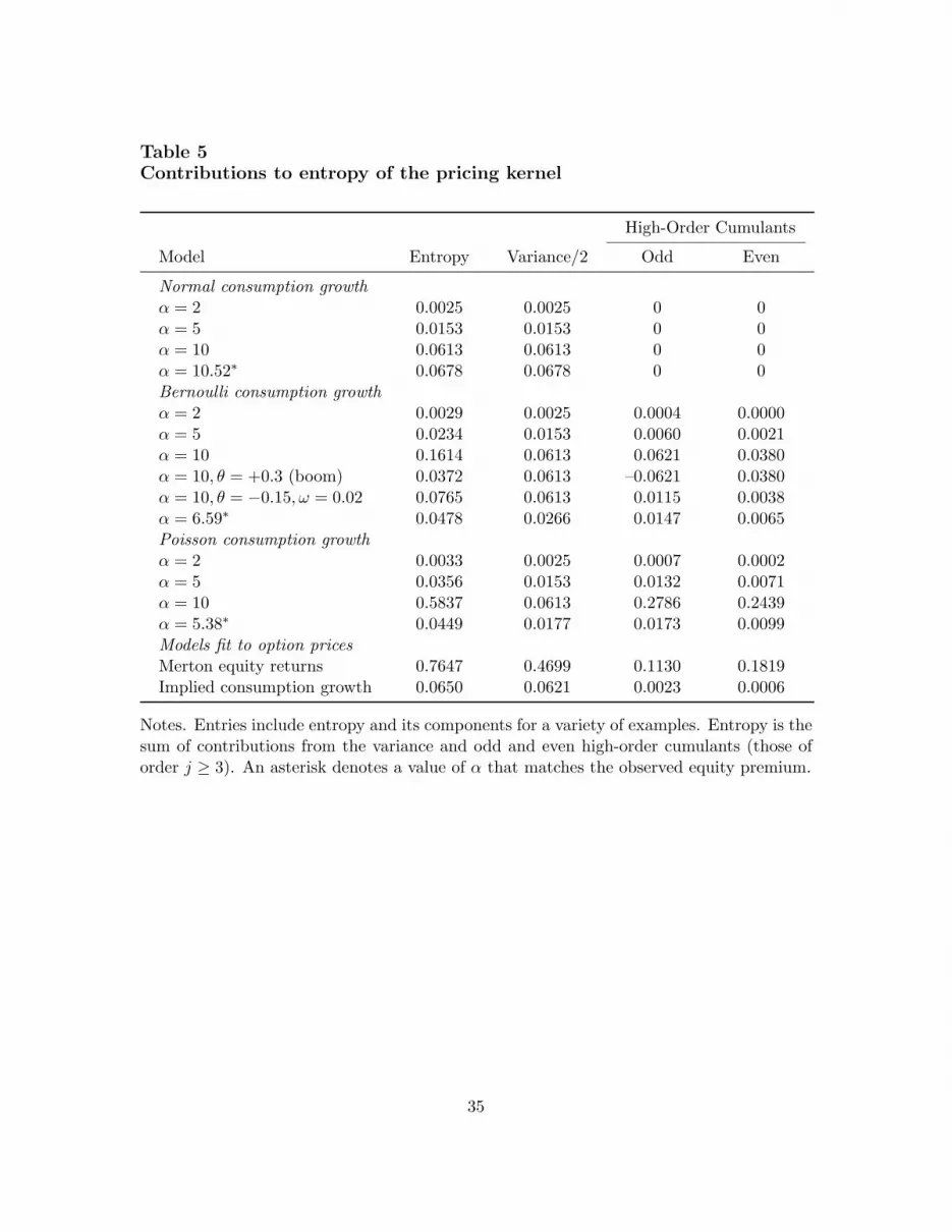
Table 5Contributions to entropy of the pricing kernel

High-Order Cumulants

Model Entropy Variance/2 Odd Even

Normal consumption growthα = 2 0.0025 0.0025 0 0α = 5 0.0153 0.0153 0 0α = 10 0.0613 0.0613 0 0α = 10.52∗ 0.0678 0.0678 0 0Bernoulli consumption growthα = 2 0.0029 0.0025 0.0004 0.0000α = 5 0.0234 0.0153 0.0060 0.0021α = 10 0.1614 0.0613 0.0621 0.0380α = 10, θ = +0.3 (boom) 0.0372 0.0613 –0.0621 0.0380α = 10, θ = −0.15, ω = 0.02 0.0765 0.0613 0.0115 0.0038α = 6.59∗ 0.0478 0.0266 0.0147 0.0065Poisson consumption growthα = 2 0.0033 0.0025 0.0007 0.0002α = 5 0.0356 0.0153 0.0132 0.0071α = 10 0.5837 0.0613 0.2786 0.2439α = 5.38∗ 0.0449 0.0177 0.0173 0.0099Models fit to option pricesMerton equity returns 0.7647 0.4699 0.1130 0.1819Implied consumption growth 0.0650 0.0621 0.0023 0.0006

Notes. Entries include entropy and its components for a variety of examples. Entropy is thesum of contributions from the variance and odd and even high-order cumulants (those oforder j ≥ 3). An asterisk denotes a value of α that matches the observed equity premium.

35

Figure 1Bernoulli disasters: cumulants of log consumption growth and contribu-tions to entropy

2 3 4 5 6 7 8 9 10−1

0

1

2x 10

−3

Cum

ulan

ts

2 3 4 5 6 7 8 9 10−2

0

2

4x 10

−3

Con

trib

utio

ns α=2

2 3 4 5 6 7 8 9 10−0.1

0

0.1

Con

trib

utio

ns α=10

Notes. The top panel summarizes the cumulants of log consumption growth, κj(log g).The next two panels summarize their contributions to the entropy of the pricing kernel,κj(log m) = (−α)jκj(log g)/j!, for risk aversion α equal to 2 and 10, respectively.

36

Figure 2Bernoulli disasters: entropy of the pricing kernel

0 2 4 6 8 10 120

0.05

0.1

0.15

0.2

0.25

0.3

0.35

0.4

Risk Aversion α

Ent

ropy

of P

ricin

g K

erne

l L(m

)

Alvarez−Jermann lower boundnormal

disasters

booms

37

Figure 3Bernoulli disasters: entropy and the equity premium

0 2 4 6 8 10 12−0.05

0

0.05

0.1

0.15

0.2

0.25

0.3

Risk Aversion α

Ent

ropy

and

Equ

ity P

rem

ium

sample mean equity premium

entropy

38

Figure 4Poisson disasters: cumulants of log consumption growth and contributionsto entropy

2 3 4 5 6 7 8 9 10−1

0

1

2x 10

−3

Cum

ulan

ts

2 3 4 5 6 7 8 9 100

1

2

3x 10

−3

Con

trib

utio

ns α=2

2 3 4 5 6 7 8 9 100

0.05

0.1

Con

trib

utio

ns α=10

Notes. See Figure 1.

39

Figure 5Poisson disasters: entropy and equity premium

0 2 4 6 8 10 12−0.5

0

0.5

1

1.5

2

Risk Aversion α

Ent

ropy

and

Equ

ity P

rem

ium

sample mean = AJ bound equity premium

entropy

40

Figure 6Implied volatility smiles for 3-month options

−0.06 −0.04 −0.02 0 0.02 0.04 0.06

0.15

0.16

0.17

0.18

0.19

0.2

Moneyness: difference of return from zero

Impl

ied

Vol

atili

ty (

annu

al u

nits

)

estimated Merton model

smaller θ*

smaller δ*

smaller δ* and positive θ*

Notes. The lines represent implied volatility “smiles” for the Merton model with estimatedparameters and some alternatives. Moneyness is measured as the difference of the returnfrom zero or, equivalently, the proportional difference of the strike from the price.

41

Figure 7Implied volatility smiles based on option and consumption data

−0.06 −0.04 −0.02 0 0.02 0.04 0.060.05

0.1

0.15

0.2

0.25

Moneyness: difference of return from zero

Impl

ied

Vol

atili

ty (

annu

al u

nits

)

consumption model (12 months)

consumption model (3 months)

option model (3 months)

option model (12 months)

42