ORIGINAL PAPER

ET mapping for agricultural water management:present status and challenges

Prasanna H. Gowda Æ Jose L. Chavez ÆPaul D. Colaizzi Æ Steve R. Evett Æ Terry A. Howell ÆJudy A. Tolk

Received: 22 March 2007 / Accepted: 16 July 2007 / Published online: 2 October 2007

� Springer-Verlag 2007

Abstract Evapotranspiration (ET) is an essential com-

ponent of the water balance. Remote sensing based

agrometeorological models are presently most suited for

estimating crop water use at both field and regional scales.

Numerous ET algorithms have been developed to make use

of remote sensing data acquired by sensors on airborne and

satellite platforms. In this paper, a literature review was

done to evaluate numerous commonly used remote sensing

based algorithms for their ability to estimate regional ET

accurately. The reported estimation accuracy varied from

67 to 97% for daily ET and above 94% for seasonal ET

indicating that they have the potential to estimate regional

ET accurately. However, there are opportunities to further

improving these models for accurately estimating all

energy balance components. The spatial and temporal

remote sensing data from the existing set of earth observing

satellite platforms are not sufficient enough to be used in

the estimation of spatially distributed ET for on-farm irri-

gation management purposes, especially at a field scale

level (*10 to 200 ha). This will be constrained further if

the thermal sensors on future Landsat satellites are aban-

doned. However, research opportunities exist to improve

the spatial and temporal resolution of ET by developing

algorithms to increase the spatial resolution of reflectance

and surface temperature data derived from Landsat/

ASTER/MODIS images using same/other-sensor high

resolution multi-spectral images.

Introduction

Evapotranspiration (ET) has been long been recognized as

the most important process that plays an essential role in

determining exchanges of energy and mass between the

hydrosphere, atmosphere and biosphere (Sellers et al.

1996). In agriculture, it is a major consumptive use of

irrigation water and precipitation on agricultural land. Any

attempt to improve water use efficiency must be based on

reliable estimates of ET, which includes water evaporation

from land and water surfaces and transpiration by vegeta-

tion. ET varies regionally and seasonally according to

weather and wind conditions (Hanson 1991). Understand-

ing these variations in ET is essential for managers

responsible for planning and management of water

resources especially in arid and semi-arid regions of the

world where crop water demand generally exceeds pre-

cipitation and requires irrigation from surface and/or

groundwater resources to meet the deficit.

At a field scale, ET can be measured over a homogenous

surface using conventional techniques such as Bowen ratio

(BR), eddy covariance (EC) and lysimeter systems. How-

ever, these systems do not provide spatial trends (or

distribution) at the regional scale especially in regions with

advective climatic conditions. Remote sensing based ET

models are better suited for estimating crop water use at a

regional scale (Allen et al. 2007a). Numerous remote

sensing-based ET algorithms that vary in complexity are

available for estimating magnitude and trends in regional

ET. This paper discusses remote sensing based regional ET

Communicated by A. Kassam.

P. H. Gowda (&) � J. L. Chavez � P. D. Colaizzi �S. R. Evett � T. A. Howell � J. A. Tolk

Conservation and Production Research Laboratory,

USDA-ARS, P.O. Drawer 10, Bushland, TX 79012, USA

e-mail: pgowda@cprl.ars.usda.gov

123

Irrig Sci (2008) 26:223–237

DOI 10.1007/s00271-007-0088-6

prediction algorithms and their limitations, data needs and

availability, knowledge gaps, and future opportunities and

challenges with respect to agriculture.

Remote sensing based ET algorithms

Remote sensing has long been recognized as the most

feasible means to provide spatially distributed regional ET

information on land surfaces (Park et al. 1968; Jackson

1984; Choudhury et al. 1987). The use of remote sensing to

estimate ET is presently being developed along two

approaches: (a) land surface energy balance (EB) method

that uses remotely sensed surface reflectance in the visible

(VIS) and near-infrared (NIR) portions of the electro-

magnetic spectrum and surface temperature (radiometric)

from an infrared (IR) thermal band, and (b) Reflectance-

based crop coefficient (generally denominated Kcr) and

reference ET approach where the crop coefficient (Kc) is

related to vegetation indices derived from canopy reflec-

tance values. The first approach is based on the rationale

that ET is a change of the state of water using available

energy in the environment for vaporization (Su et al. 2005).

Remote sensing based EB models convert satellite sensed

radiances into land surface characteristics such as albedo,

leaf area index, vegetation indices, surface emissivity and

surface temperature to estimate ET as a ‘‘residual’’ of the

land surface energy balance equation:

LE ¼ Rn � G� H ð1Þ

where, Rn is the net radiation resulting from the budget of

short and long wave incoming and emitted radiation

respectively, LE is the latent heat flux from evapotranspi-

ration, G is the soil heat flux, and H is the sensible heat flux

(all in W m–2 units). LE is converted to ET (mm h–1 or

mm day–1) by dividing it by the latent heat of vaporization

(kv; *2.45 MJ kg–1) and an appropriate time constant. Rn

and G may be estimated locally using meteorological

measurements (Allen et al. 1998) and regionally by

incorporating spatially distributed reflected and emitted

radiation (Jackson et al. 1985) as:

Rn ¼ ð1� aÞ Rs þ ea r T4a � es r T4

s ð2Þ

where a is surface albedo, Rs is incoming short wave

radiation (W m–2) measured with pyranometers or calcu-

lated using the Angstrom formula based on the solar

constant, location and time of the year (Allen et al. 1998)

or by using the solar constant, the cosine of the solar

incidence angle, the inverse squared relative earth–sun

distance, and atmospheric transmissivity based on the area

of interest (image) ground elevation respect to mean sea

level (Allen et al. 2007a), r is the Stefan–Boltzmann

constant (5.67 E-08 W m–2 K–4), e is emissivity and T

temperature (K) with subscripts ‘‘a’’ and ‘‘s’’ for air and

surface, respectively. Ts is the remotely sensed radiometric

surface temperature which is obtained after correcting the

sensor brightness temperature imagery for atmospheric

effects and for surface emissivity considering, for example,

procedures by Hipps (1989) and Brunsell and Gillies

(2002). The surface emissivity correction is performed

assuming typical bare soil and fully vegetated surface

emissivities of 0.93 and 0.98, respectively, and the frac-

tional vegetation cover from the scaled normalized

difference vegetation index (NDVI). Alternatively, surface

albedo for vegetated areas is generally estimated using the

Brest and Goward (1987) model. This model is based on

the red (R) and NIR band reflectance:

a = 0.512 Rþ 0.418 NIR ð3Þ

The emissivity of air can be obtained from the Brutsaert

(1975) equation:

ea ¼ 0:0172ea

Ta

� �1=7

ð4Þ

where ea is actual vapor pressure (kPa). G is commonly

estimated as a fraction of Rn depending on leaf area index

(LAI) or NDVI. Chavez et al. (2005) found that a

combination of a linear and a logarithmic model could

estimate G for soils planted to corn and soybean crops in

central Iowa (r2 = 0.73):

G ¼ Rn ð0:3324� 0:024 LAIÞð0:8155� 0:3032 LNðLAIÞÞð5Þ

H is then estimated using the aerodynamic surface–air

temperature gradient (or combination of gradients) and

aerodynamic resistance, where generally radiometric

temperature (Ts) has been used as a surrogate for

aerodynamic temperature (To).

In the second approach, R and NIR reflectance mea-

surements are used to compute a vegetation index such as

NDVI (Rouse et al. 1974) or the soil adjusted vegetation

index (SAVI; Huete 1988), and the vegetation index is then

used in place of calendar days or heat units to drive or scale

the crop coefficient. The reference ET is then computed

using local meteorological measurements of incoming

solar radiation, air temperature, relative humidity or dew

temperature, and wind speed.

Some early applications of remote sensing based EB

models include Brown and Rosenberg (1973), Brown

(1974), Stone and Horton (1974), Idso et al. (1975),

Heilman et al. (1976), Verma et al. (1976), Kanemasu

et al. (1977), and Jackson et al. (1977). Most of these

studies used airborne scanners as first demonstrated by

224 Irrig Sci (2008) 26:223–237

123

Bartholic et al. (1972). Price (1982), Seguin and Itier

(1983), and Taconet et al. (1986) were among some of the

first to use thermal data obtained from satellites to esti-

mate ET. They proposed to use surface temperature

derived from remotely sensed data to estimate regional

ET in the form:

LE ¼ Rn � G� qa CpðTs � TaÞrah

ð6Þ

where qa is air density (kg m–3), Cp is specific heat

capacity of the air (J kg–1 K–1), and rah is aerodynamic

resistance for heat transfer (s m–1). Ts and Ta are expressed

in K. For example, Brown and Rosenberg (1973), and

Brown (1974) used the surface radiometric temperature

and air temperature difference, (Ts – Ta), and the aerody-

namic resistance (rah) to estimate H where the canopy or

surface temperature was obtained from remotely sensed

radiometric temperature using thermal scanners having a

bandwidth mostly in the range of 10–12 lm. Later,

Rosenberg et al. (1983) incorporated the term surface

aerodynamic temperature (To) in the H model, instead of

surface radiometric temperature, considering that the tem-

perature gradient (for H) was a gradient between air

temperature within the canopy (at a height equal to the zero

plane displacement plus the roughness length for heat

transfer) and air temperature above the canopy (at a height

where wind speed was measured or height for rah). They

indicated that for partially vegetated areas and for water

stressed biomass, radiometric and aerodynamic tempera-

tures of the surface were not equal. This inequality is

discussed further in a later section.

Hatfield et al. (1983) evaluated the surface temperature

with the energy balance approach at seven locations

throughout the United States equipped with weighing

lysimeters and ground-based instrumentation. In their

study, daily G was assumed negligible. Crops were sor-

ghum, alfalfa, tomato and wheat at full cover, and tomato

at 80% cover. They concluded that remotely sensed Ts may

be used in the EB model to estimate regional ET. Estimated

LE values, using atmosphere stability corrected aerody-

namic resistances, were very closely matched to those

measured by the lysimeters. Reginato et al. (1985) refined

estimates of Rn using reflected shortwave and emitted long

wave measurements as outlined by Jackson et al. (1985).

They also used ground-based instrumentation to estimate

ET of wheat and achieved good agreement with lysimeters

and neutron scattering. Later, Jackson et al. (1987) applied

this procedure using an airborne radiometer and compared

with BR measurements for cotton, alfalfa, and wheat with

homogenous crop surfaces (full canopy with no contribu-

tion from soil background). Comparison of the remote

sensing based LE estimates for 5 days with BR values

resulted in a greatest difference of 12% while errors in

daily ET estimates were less than 8% for 3 days and 25%

on the other two. Moran et al. (1989) then applied this

procedure using R/NIR (simple ratio) and thermal data

from the Landsat Thematic Mapper (TM) satellite and

reported agreement within 12% with the BR and airborne

data from Jackson et al. (1987).

Accurate estimates of H are very difficult to achieve,

mainly when Ts is used instead of To and when atmospheric

effects and surface emissivity are not considered properly.

In such cases, H prediction errors have been reported to be

around 100 W m–2 (Chavez and Neale 2003; Matsushima

2000). Consequently, more recent EB models differ mainly

in the manner that H is estimated. These models included

the two-source model (TSM; Norman et al. 1995; Kustas

and Norman 1996; Chehbouni et al. 2001), where the

energy balance of soil and vegetation are modeled sepa-

rately and then combined to estimate total LE, surface

energy balance algorithm for land (SEBAL; Bastiaanssen

et al. 1998) that uses hot and cold pixels to develop an

empirical temperature difference equation, and surface

energy balance index (SEBI; Menenti and Choudhury

1993) based on the contrast between wet and dry areas.

Other models include simplified surface energy balance

index (S-SEBI; Roerink et al. 2000); surface energy bal-

ance system (SEBS; Su 2002); the excess resistance (kB–1;

Kustas and Daughtry 1990; Su 2002); the aerodynamic

temperature parameterization models proposed by Crago

et al. (2004) and Chavez et al. (2005); Beta (b) approach

(Chehbouni et al. 1996); and most recently ET mapping

algorithm (ETMA; Loheide and Gorelick 2005) and

Mapping Evapotranspiration with Internalized Calibration

(METRICTM; Allen et al. 2002, 2005, 2007a). The sections

below discuss the main models in detail.

SEBI, SEBS and S-SEBS: SEBI, proposed by Menenti

and Choudhury (1993), is based on the crop water stress

index (CWSI; Jackson et al. 1981) concept in which sur-

face meteorological scaling of CWSI is replaced with

planetary boundary layer (PBL) scaling. It uses the contrast

between wet and dry areas appearing within a remotely

sensed scene to derive ET from the relative evaporative

fraction (Kr). It determines Kr by relating surface temper-

ature observations to theoretical upper and lower bounds

on the difference between surface and air temperature

(Menenti et al. 2003). Evaporative fraction (K), as utilized

by Bastiaanssen et al. (1998), is defined as the ratio of

latent heat flux to the available energy (AE = Rn – G) and

is assumed to remain nearly constant during the day.

Surface energy balance system (Su 2002) was developed

using the SEBI concept. It uses a dynamic model for

thermal roughness (Su et al. 2001), bulk atmospheric

similarity (BAS) (Brutsaert 1999) and Monin–Obukhov

similarity (MOS) theories for regional ET estimation, and

atmospheric surface layer (ASL) scaling for estimating ET

Irrig Sci (2008) 26:223–237 225

123

at local scale. SEBS requires wet and dry boundary con-

ditions to estimate H. Under dry conditions, the calculation

of Hdry is set to the available energy AE as evaporation

becomes zero due to the limitation of water availability and

Hwet is calculated using the Penman–Monteith parameter-

ization (Monteith 1965, 1981) as:

Hwet ¼ AE�qa Cp

rah

� �es � e

c

� �

1þ Dc

� � ð7Þ

where e is the actual vapor pressure (kPa), es is the

saturation vapor pressure (kPa), c is the psychrometric

constant (kPa �C–1), D is the rate of change of saturation

vapor pressure with temperature (kPa �C–1) and rah is the

bulk surface external or aerodynamic resistance (s m–1)

estimated under the assumption that the bulk internal

resistance is zero. Finally, relative evaporative fraction

(Kr), evaporative fraction (K) and LE for each pixel in the

remote sensing image is calculated as:

Kr ¼ 1� H � Hwet

Hdry � Hwet

ð8Þ

K ¼ KrðRn � G� HwetÞRn � G

ð9Þ

and

LE ¼ KðRn � GÞ ð10Þ

The evaporative fraction (K = LE/(Rn – G)) is used in

the estimation of LE because it is assumed to remain

constant through out the day and can be obtained for

short periods and be used for LE extrapolation to daily

values. Brutsaert and Sugita (1992) presented the

assumption that the partitioning of available energy (AE)

into H and LE is constant (self-preservation of the available

energy partitioning) or that the evaporative fraction remains

almost constant during the daytime. Zhang and Lemeur

(1995) added that the evaporative fraction indicates how

much of the available energy is used for ET and that the

assumption that the instantaneous K is representative of the

daily energy partitioning, is an acceptable approximation

for clear-sky conditions. Crago (2000) concluded that the Khas the tendency to be nearly constant during daytime,

permitting the estimation of daytime evaporation from one

or two estimates of the evaporative fraction during the

middle of the day at the satellite overpass time.

Su et al. (2005) evaluated SEBS with two independent,

high-quality datasets that were collected at a field scale

during the soil moisture–atmosphere coupling experi-

ment (SMACEX) in the Walnut Creek agricultural

watershed near Ames, IA, USA. Meteorological and EC

measurements from ten locations within the watershed

were used to estimate and compare fluxes during a period

of rapid vegetation growth and varied hydrometeorology.

Results indicated that ET estimates from the SEBS were

close to 85–90% of the measured ET values from EC

systems for both corn and soybean surfaces. In the same

study, regional fluxes were calculated using Landsat

enhanced thematic mapper plus (ETM+) data for a clear

day during the field experiment. Results at the regional

scale showed that ET prediction accuracies were strongly

related to crop type with improved ET estimates for corn

surfaces compared to those of soybean. Differences

between the observed and predicted ET values were

approximately 5%. Further, McCabe and Wood (2006)

used thermal data from Landsat ETM+ (60 m), advanced

spaceborne thermal emission and reflection radiometer

(ASTER; 90 m), and moderate resolution imaging spec-

trometer (MODIS; 1,020 m) sensors to independently

estimate ET using SEBS. A high degree of consistency

was observed between flux retrievals from ETM+ and

ASTER data while MODIS data was unable to discrim-

inate the influence of heterogeneity in land use at field

scale. The main limitation with the SEBS is that it

requires aerodynamic roughness height. Currently, several

methods are available to estimate this variable using wind

profile, vegetation index, and crop height (hc in m) or by

assigning nominal values based on the land use.

S-SEBI (Roerink et al. 2000) is a simplified method

derived from SEBS to estimate surface fluxes from remote

sensing data. Consequently, this model is based on K and

the contrast between the areas with extreme wet and dry

temperature, Twet and Tdry, respectively. The instantaneous

LE is calculated as:

LEi ¼ KiðRn � GÞi ð11Þ

where the subscript ‘‘i’’ means instantaneous. Ki is

expressed as:

Ki ¼TDry � TS

TDry � TWet

ð12Þ

Ki is assumed constant through the day. Daily LE (LEd) is

calculated as:

LEd ¼LEi Rn;d

ðRn � GÞið13Þ

where Rn,d is daily net radiation (W m–2), can be estimated

from a known relationship at solar noon as:

Cd;i ¼Rn;d

Rn;ið14Þ

226 Irrig Sci (2008) 26:223–237

123

where Rn,i is the instantaneous net radiation, and Cd,i is

approximately 0.30 (±0.03) for summer months. Finally,

ETd can be estimated as:

ETd ¼Ki Cd;i Rn;i

kv ð15Þ

The disadvantage of this method may be that it requires

extreme Ts values, which cannot always be found on every

image. However, the major advantages are that it is a

simpler method that does not need additional meteorological

data and it does not require roughness length as in the case

of SEBS. Gomez et al. (2005) used the K concept based

on S-SEBI for estimating ETi and to extrapolate it to ETd.

The method was applied using airborne sensor: PolDER

(polarization and directionality of earth reflectance) and

a thermal camera. Validation with a BR system showed

LE estimation error of 26% and 1 mm day–1 for ETd over

corn, alfalfa, wheat and sunflower crops.

TSM: The TSM considers the energy balance of the

substrate (e.g., soil) and vegetation components separately,

and then combines these components to estimate total ET.

Norman et al. (1995) and Kustas and Norman (1999)

developed operational methodology to the two-source

approach proposed by Shuttleworth and Wallace (1985) and

Shuttleworth and Gurney (1990). This methodology gen-

erally does not require additional meteorological or

information over single-source models; however, it requires

some assumptions such as the partitioning of composite

radiometric surface temperature into soil and vegetation

components, turbulent exchange of mass and energy at the

soil level, and coupling/decoupling of energy exchange

between vegetation and substrate (i.e., parallel or series

resistance networks). The energy exchange in the soil–

plant–atmosphere continuum is based on resistances to heat

and momentum transport, and sensible heat fluxes are

estimated by the temperature gradient–resistance system.

Radiometric temperatures, resistances, sensible heat fluxes,

and latent heat fluxes of the canopy and soil components are

derived by iterative procedures constrained by composite,

directional radiometric surface temperature, vegetation

cover fraction, and maximum potential latent heat flux.

Kustas et al. (2004) applied TSM to Landsat TM and

ETM+ images to evaluate the effect of sensor resolution on

model output over corn and soybean fields in central Iowa.

The pixel resolution was varied from 60–120, 240, and

960 m. Comparison of flux estimates with tower-based and

aircraft-based flux measurements indicate that the TSM

performed reasonably well. Gonzalez-Dugo et al. (2006)

compared an EB single-source model with TSM to evalu-

ate their ability to estimate surface fluxes. They found that

both methods performed well (RMSD less than 31 W m–2)

in estimating the H using calibrated Landsat TM imagery.

However, the TSM performed slightly better than the EB

single source model with r2 values of 0.87 and 0.94 for H

and LE estimates, respectively. The EB single source

model produced r2 values of 0.78 and 0.91 for H and LE

estimates, respectively. Colaizzi et al. (2006a) evaluated

the TSM for alfalfa, corn, cotton, grain sorghum, soybeans,

winter wheat, wheat stubble, and bare soil using large

weighing lysimeters in Bushland, Texas. The TSM over-

estimated LE for smaller observed LE (\|400| W m–2) by

up to 200 W m–2, but relative error improved for larger

LE. Overall, RMSE ranged from 77 W m–2 for soybean to

135 W m–2 for winter wheat, and TSM performance was

not influenced by regional advection.

Norman et al. (2000a, b) proposed a variation of the

TSM called dual-temperature-difference (DTD) method

using time rate of change in Ts and Ta to compute surface

heat fluxes. This method reduced the effect of errors

associated with radiometric calibration, emissivity varia-

tions, and use of non-local air temperature and wind speed

data. Comparison of H estimates from DTD method with

that from original TSM indicated that the DTD method had

potential for regional-scale applications using geo-station-

ary satellites (like GOES) data with a synoptic weather

network. H estimation errors were generally \50 W m–2.

The DTD approach was well suited for geostationary sat-

ellites with high temporal resolution but coarse (4 km)

spatial resolution, and it conceivably could be applied to

thermal pixel disaggregation schemes to improve spatial

resolution such as those described in the below paragraph.

Using the TSM, Kustas et al. (2003) and Norman et al.

(2003) developed a two-step approach called the Disag-

gregated Atmosphere Land EXchange Inverse model

(DisALEXI) to combine low- and high-resolution remote

sensing data to estimate ET on the 10–100 m scale without

requiring local observations. The first step involves deriv-

ing surface fluxes from low spatial resolution but

frequently available remote sensing data using a coupled

TSM–ABL model known as ALEXI. The second step di-

saggregates those low spatial resolution surface flux

estimates using vegetation index and surface temperature

estimates derived from non-frequent high resolution

remote sensing datasets. For example, one can derive

average surface flux estimates from a 4-h repeat cycle

GOES satellite data with a spatial resolution of 5 km and

disaggregate into high spatial resolution flux maps using

vegetation index and surface temperature data from

Landsat (30 m) dataset with a repeat cycle of 16 days.

They successfully demonstrated its application using data

from the Southern Great Plains in central Oklahoma

(Norman et al. 2003). The root mean square difference

(RMSD) between remote sensing estimates of surface

fluxes and ground-based measurements were within 10–

Irrig Sci (2008) 26:223–237 227

123

12%. Similar results were reported by Anderson et al.

(2007).

SEBAL: Bastiaanssen (1995) and Bastiaanssen et al.

(1998, 2005) described SEBAL in detail. Briefly, SEBAL

is essentially a single-source model that solves the EB for

LE as a residual. Rn and G are calculated based on Ts and

reflectance-derived values of albedo, vegetation indices,

LAI and surface emissivity. H is estimated using the bulk

aerodynamic resistance model and a procedure that

assumes a linear relationship between the aerodynamic

surface temperature–air temperature difference (dT) and

radiometric surface temperature (Ts) calculated from

extreme pixels. Basically, extreme pixels showing cold and

hot spots are selected to develop a linear relationship

between dT and Ts. At the cold pixel in the satellite

imagery, H is assumed non-existent i.e., Hcold = 0 and at

the hot pixel, LE is set to 0 which in turn allows to set

Hhot = (Rn – G)hot. Then, dTcold = 0 and dThot can be

obtained by solving the bulk aerodynamic resistance

equation for the hot pixel as:

H ¼ qaCPdT

rah

ð16Þ

After calculating dT at both cold and hot pixels, a linear

relationship between dT and Ts is developed to estimate H

iteratively correcting rah for atmospheric stability. This is

done applying the MOS theory. This step requires Ta and u

measured at a weather station and a mechanism that

extrapolates wind speed to a blending height of 100–

200 m. The dT artifice is expected to compensate for errors

in surface temperature estimates due to atmospheric

correction, and does not assume that radiometric and

aerodynamic temperatures are equivalent.

SEBAL has been tested extensively in different parts of

the world. Bastiaanssen et al. (2005) summarized SEBAL

accuracy under several climatic conditions at both field and

regional scales. For a range of soil wetness and plant

community conditions, the typical accuracy at field scale

was 85% for a single day and 95% for a seasonal scale. For

large watersheds, on an annual basis, the ET prediction

accuracy was up to 96%. However, application of SEBAL

by Trezza (2002) for a variety of crops in Kimberly, ID

resulted in ET estimation errors ranging from 2.7 to 35%

with an average error of 18.2%.

METRICTM: A full description of the METRICTM can be

found in Allen et al. (2002, 2005, 2007a) who highlighted

that METRICTM uses remote sensing imagery in the visi-

ble, near-infrared and thermal portion of the electro-

magnetic spectrum along with ground-based horizontal

wind speed and near surface dew point temperature mea-

surements. This model is based on the SEBAL algorithm.

The main difference between SEBAL and METRICTM is

that the latter does not assumes H = 0 or LE = Rn – G at

the wet pixel, instead a soil water budget is applied for the

hot pixel to verify that ET is indeed zero and for the wet

pixel, LE is set to 1.05 ETr kv, where ETr is the hourly (or

shorter time interval) tall reference (like alfalfa) ET cal-

culated using the standardized ASCE Penman–Monteith

equation. The second difference is that it selects extreme

pixels purely in an agricultural setting whereby the cold

pixel should have biophysical characteristics (e.g., hc, LAI)

similar to the reference crop (alfalfa). The third difference

is that METRICTM uses the alfalfa reference evapotrans-

piration fraction (ETrF) mechanism to extrapolate

instantaneous LE flux to daily ET rates instead of using the

K. ETrF is the ratio of ETi (remotely sensed instantaneous

ET) to the reference ETr (e.g., mm h–1) that is computed

from weather station data at overpass time.

Tasumi et al. (2003) validated METRICTM for various

crops grown on weighing lysimeters located at the USDA-

ARS laboratory in Kimberly, Idaho. Allen et al. (2007b,

2005) compared seasonal ET estimated for two agroeco-

systems in Idaho: an irrigated meadow in the Bear River

Basin and a sugar beet field near Kimberly, using MET-

RICTM with lysimeters measurements resulted in 4 and 1%

errors, respectively; with ET overestimation errors as high

as 10–20%. Errors in predicted monthly ET at Montpelier,

ID averaged ±16% relative to a local lysimeter, although

the difference for ET sums over a 4-month period was only

4%, according to the authors. Chavez et al. (2007) applied

METRICTM to the Texas High Plains using a Landsat 5

TM image acquired early in the cropping season. The

performance of the METRICTM was evaluated by com-

paring the predicted daily ET with values derived from a

soil water budget at four different locations. ET estimates

errors were below 15%. The use of METRICTM for the

advective conditions of the Texas High Plains is promising;

however, more evaluation is needed using lysimeter or

well-calibrated Scintillometer derived ET measurements

for different agroclimatological conditions.

ETMA: The ETMA proposed by Loheide and Gorelick

(2005) is based on the surface energy budget and requires

only local weather data including G measurements and

high-resolution airborne thermal imagery to estimate ET. It

uses two surface temperature points, TLE and TH, at which

all of the turbulent heat flux is attributed to the LE and H,

respectively, to develop linear relationships between sur-

face temperature and instantaneous ET (ETi) at specified

times as follows:

ETi ¼ AE

TH�TS

TH�TLE

� �kv : ð17Þ

228 Irrig Sci (2008) 26:223–237

123

At H = 0, TLE = Ta and at LE = 0, the TH is calculated as:

TH ¼AE ðrah þ rexÞ

qa Cpþ Ta ð18Þ

where rex is the excess resistance that is encountered for

heat transfer compared to momentum transfer (Norman and

Becker 1995). Daily ET will then be developed from two

instantaneous ET maps using Penman–Montieth and Jarvis–

Stewart models and surface resistance. ETMA was intended

for application at the local scale where Ta, u, hc, e, and Tsoil,

are uniform in space. This model may not work well for

regions subject to advective conditions or may not be

applicable on regions with significant surface heterogeneity.

EB methods based on relating To to Ts: Since To cannot

be measured directly, it is usually derived by inverting

some form of Eq. (6). Numerous studies have shown that Ts

and To are neither equal nor do they have a unique rela-

tionship, as reviewed by Kustas et al. (2003, 2007). Kustas

and Norman (1996) pointed out that the difference between

Ts and To can be significant for relatively sparse vegetation

cover (LAI \ 1.5) and/or water stressed vegetation.

Chehbouni et al. (1996) tried to compensate for the

difference of these two temperatures by trying to relate

(Ts – To) to (Ts – Ta) for grass and mesquite patches. They

indicated that despite some scatters, especially for the

mesquite site, the comparison showed that the (Ts – To)

increased as To increased. Their model assumed that the

relationship was not linear. Their results allowed the for-

mulating of sensible heat flux (H) using Ts as:

H ¼ qa Cp bTs � Ta

rah

� �ð19Þ

where,

b ¼ 1

exp LL�LAI

� �� 1

ð20Þ

where L is a site-specific empirical factor. In Chehbouni

et al. (1996), L was found to be 2.5 through least square

regression. They calibrated the model for LAI values less

than 1.0 m2 m–2. A similar study by Matsushima (2005)

over a wide range of rice density (LAI ranged from 0.04 to

5.4) indicated that the variation of b with LAI did not agree

with the empirical parameterization proposed by Chehbo-

uni et al. (1996). Instead, the author found that the

logarithmic diurnal average of the thermal roughness

lengths (Zoh) was a function of LAI. While on the other

hand, Colaizzi et al. (2004) compared (Ts – Ta) with

(To – Ta) using weighing lysimeters planted with irrigated

alfalfa, irrigated and dryland cotton, and dryland grain

sorghum. They did not find a relationship between

(Ts – Ta) and (To – Ta). They concluded that the difference

might have been influenced by the different surface

roughness of each crop type.

Zibognon et al. (2002) applied a land surface–atmo-

sphere-radiometer model to convert Ts to an equivalent

isothermal (or aerodynamic) temperature using data for one

day at a grass site with LAI of 1.0. The model used vari-

ables that described the shape of the vertical foliage

temperature profile. The model estimates were compared to

the To reference values from the inversion of the MOS

theory, obtaining good agreement. In this study, To over Ts

resulted in an improvement by 3.6 K.

Crago et al. (2004) suggested calibrating the bulk

aerodynamic resistance equation (Rosenberg et al. 1983) to

estimate To, using estimated H values with the analytical

land–atmosphere-radiometer model (ALARM). The model

assumed the foliage had an exponential vertical tempera-

ture profile. They indicated that the same profile was felt by

the within-canopy turbulence. The ALARM converted

radiometric surface temperatures into To called the equiv-

alent radiometric isothermal surface temperature and then

calculated H using the MOS theory.

Chavez et al. (2005) linearly related aerodynamic tem-

perature (To) to Ts, LAI, Ta and u for corn and soybean fields

in central Iowa. The calibration equation resulted with an

r2 value of 0.77. The linear expression is shown below:

To ¼ 0:534 Ts þ 0:39 Ta þ 0:244 LAI� 0:192 uþ 1:67

ð21Þ

where Ts and Ta are in �C, LAI is in m2 m–2, and u is in

m s–1. EC systems were used to extract values for u and Ta.

The model was found to be valid for a LAI range of 0.3–5.0

and u values ranging from 1.5 to 7.3 m s–1. Ta was mea-

sured approximately at a height of 2 m for soybean and

3 m for corn.

The evaluation of the To model was performed with

inverted values from measured H using a different set of

EC stations resulted in a mean bias error (MBE) and root

mean square error (RMSE) values of 0.2 and 0.9 �C,

respectively. The corresponding goodness of fit was

r2 = 0.90 which demonstrated the good agreement with

measured values. The To model was used in the EB esti-

mation of LE which was compared to EC measured values

resulting in MBE and RMSE of –9.2 and 39.4 W m–2,

respectively. The errors were well within the margin of

errors of the LE from EC ground station measurements.

The comparison of estimated with measured values was

performed taking into account the heat fluxes footprint by

means of heat flux source area models that incorporate the

analytical solution to the diffusion–dispersion–advection

equation. However, note that the To model was developed

using data over corn and soybean fields having relatively

homogeneous surface canopies under unstable atmospheric

Irrig Sci (2008) 26:223–237 229

123

conditions. Therefore, the proposed model requires further

evaluation over heterogeneous surfaces and/or under sta-

ble/neutral atmospheric conditions of semi-arid regions.

Instantaneous to daily ET extrapolation

This technique was first introduced by Jackson et al. (1983)

to calculate a coefficient to convert one-time-of-day remote

sensing based ET estimates to daily total ET. It required

geographic latitude, day of year, and time of day and diurnal

solar radiation and ET were described by a sine function.

They compared ET estimates with lysimetrically determined

daily total ET for four crops at five different locations.

Results indicated that reliable estimates of daily ET from

one-time-of-day measurements could be made for cloud free

days. For cloudy days, the results were less reliable, but the

authors suggested that estimates could be improved by

considering the amount and temporal distribution of cloud

cover. They added that the one-time-of-day measurements

should be made within about 2 h of solar noon.

In a recent study on fully irrigated alfalfa, partially

irrigated cotton, dryland grain sorghum and bare soil (tilled

fallow sorghum), Colaizzi et al. (2006b) found that the

ETrF approach could scale instantaneous LE to daily ET

more accurately for cropped surfaces compared with

evaporative fraction [K = LE/(Rn – G)]; however, K gave

slightly better prediction for bare soil. The authors used the

standardized ASCE-PM grass reference ET (EToF) to scale

daily ET from one-time-of-day 0.5 h ET data from a

lysimeter. They found daily ET underestimation errors

were within the 10% for ET [ 6 mm day–1, within 20%

for ET values between 3.9 and 5.8 mm day–1, and [20%

for ET values ranged 0.4–3.2 mm day–1. In a airborne

remote sensing study conducted in Walnut Creek water-

shed located south of Ames in central Iowa, Chavez and

Neale (2007) compared evaporative fraction, the solar

radiation method and the alfalfa and grass reference

evapotranspiration fraction methods to extrapolate instan-

taneous to daily ET. Instantaneous ET estimates were made

from aircraft imagery acquired at different times of the day.

In the study area, plant available water was not a limiting

factor and advection was not an issue. Results indicated

that the K method performed better than the other two

methods when compared to daily ET values measured by

several EC systems. Better results were obtained for flight

overpasses from local Noon to close to 2:00 PM CST.

Reflectance-based crop coefficient method

Reflectance based crop coefficient method has been studied,

among others, by Reginato et al. (1985), Neale et al. (1989,

2003), and Hunsaker et al. (2005). Furthermore, crop

coefficients (Kc) have been related to vegetation indices

such as PVI (Jackson et al. 1980; Heilman et al. 1982),

NDVI (Bausch and Neale 1987; Neale et al. 1989), and

SAVI (Bausch 1993; Neale et al. 1996). D’Urso and Santini

(1996) attempted to derive the crop coefficient analytically

from remote sensing estimated albedo, surface roughness,

and aerodynamic resistance (from LAI). This method does

not require knowledge of crop development stage.

Kc is defined by the ratio of the crop ETc to the reference

crop ET (grass or alfalfa). According to Allen et al. (1998),

Kc represents an integration of the effects of four charac-

teristics that distinguish a given crop form the reference

crop: crop height (affects aerodynamic resistance and

vapor transfer), canopy-soil albedo (affects Rn), canopy

resistance (to vapor transfer), and evaporation from soil. Kc

is mainly directly derived from studies of the soil water

balance determined from cropped fields or from lysimeters.

Kc values are estimated under optimal agronomical con-

ditions, i.e., no water stress, disease, weed/insect

infestation, or salinity issues.

Neale et al. (1996), using multi-temporal airborne digital

multi-spectral video imagery acquired over cotton crop

through a growing season, obtained reflectance-based crop

coefficients that were related to the SAVI. They maintained

a water balance in the root zone of the cotton crop in three

fields with ET estimates based on Kc derived using the

spectral methods and Kc curves from FAO Paper No. 56

(Allen et al. 1998). Reflectance based Kc followed the

actual cotton growth in the field. Their results indicated

that the FAO’s Kc procedure underestimated ET during the

vegetative stage of growth and overestimated towards the

latter in the cropping season. Based on a simulated irri-

gation schedule, they emphasized that water savings could

have been up to 12%. Similarly, Harikishan et al. (2006)

used the basal crop coefficient (Kcb) approach to estimate

the crop ET from a non-water limited soil–plant environ-

ment showing a dry soil surface and plants free of pest/

disease. They concluded that canopy reflectance-based

crop coefficient is a practical and accurate indicator of the

actual crop ET. They conducted root zone soil water bal-

ance simulations where the seasonal variations in the

simulated soil water profiles in the root zone were com-

pared to the actual soil water contents measured with a

neutron probe. Results showed good agreement throughout

the cropping season and validated the canopy reflectance-

based crop coefficient for non-grain crops. A historical

retrospective on the remote sensing based crop coefficients

for ET can be found in Neale et al. (2003). They concluded

that the remote sensing based crop coefficients can be

accurately used for grain, non-grain and forage crops.

In Kenya, Michael and Bastiaanssen (2000) derived

reflectance based crop coefficient (Kcr) from Landsat

230 Irrig Sci (2008) 26:223–237

123

images using the simplified Priestley–Taylor equation for

estimating crop ET. They obtained good results for un-

stressed crop where vapor pressure deficits remained within

acceptable limits. Tasumi et al. (2005a, b, 2006) showed a

method to estimate Kcr using a satellite-based EB model

and a parameterization of Kcr (which in this case repre-

sented mean Kc) using NDVI to obtain daily ET. With this

method traditional Kcr curves could be adjusted to reflect

actual crop/weather/field/management conditions by shift-

ing key crop development days (curve shifting) to better

match the remote sensing based Kcr curve and to obtain

improved ET estimates. With the parameterization of Kcr

using NDVI, ET estimates for grass and sugar beets were

compared to lysimeter measurements. The seasonal ET

estimation errors for grass and sugar beets were 2 and 6%,

respectively. The method of calibration was region specific

and did not need a land use map showing crop types.

On a different approach, Zhang and Wegehenkel (2006)

developed a regional ET model that integrates the MODIS

vegetation data (VIS, NIR reflectance) with the FAO-56

Penman–Monteith reference ET model, where Kc was

estimated based on the crop hc and fractional vegetation

cover (fc). Fractional vegetation cover was related to NDVI

values and root depth to LAI through the season. Estimated

seasonal ET was compared with ET by twelve lysimeters

(1 m2 · 1.5 m deep) in Berlin, Germany, resulting in an

index of agreement above 0.87 and R2 values higher than

0.59.

In a semi-arid region of Morocco, Er-Raki et al. (2007)

compared estimates of actual ET for winter wheat under

different irrigation treatments; using Kcb values from the

FAO-56 procedure, locally measured Kcb, and Kcb and fcderived from NDVI (reflectance values based on ground

radiometer readings); with ET values derived from EC

systems. At mid-season state, the Kcb values based on

FAO-56 were found considerably less than the locally

calibrated Kcb values. NDVI-based Kcb values were found

acceptable especially when the soil evaporation was neg-

ligible suggesting that this method is promising for

regional scale ET estimation. The locally developed Kcb

values and the NDVI based values performed similarly

with ET prediction errors of 0.16 ± 0.45 and

0.33 ± 0.51 mm day–1, respectively, producing a model

efficiency of 79 and 70%, respectively, compared to 44%

with the FAO-56 procedure.

Limitations and future challenges

Radiometric versus aerodynamic temperature

It was recognized that radiometric temperature is sensitive

to canopy structure (Kimes 1980), vertical vegetation

temperature distribution (Kimes et al. 1980), and row

spacing and soil–vegetation component temperatures

(Kimes 1983), regardless of the type of platform used

(i.e., ground, airborne, or satellite) or sensor characteristics

(i.e., band pass response, field of view, internal calibra-

tion). Most single-source EB methods use radiometric

temperature as a surrogate for To although they may not be

equal. Greater differences between Ts and To may be found

with larger BRs (i.e., when the sensible heat flux is much

larger in proportion to latent heat flux), and with partial

vegetation (Hatfield et al. 1984; Jackson et al. 1987) and

dry or water stressed vegetation (Kustas et al. 1989; Kalma

and Jupp 1990). Norman et al. (1995) and Norman and

Becker (1995) pointed out that when two targets (e.g., soil

and vegetation) at different temperature levels are viewed

by the sensor, their composite wavelength distribution is

not that of a blackbody, meaning that there is no equivalent

composite blackbody giving the same radiance at the given

temperature. Hence, equality of radiometric and aerody-

namic temperature, at least for composite surfaces, should

not be expected. Supporting these findings, Alves et al.

(2000) found that radiometric surface temperature for dry

conditions greatly depart from the aerodynamic tempera-

ture, which in turn will result in considerable errors in the

estimation of sensible heat flux.

Spatial and temporal resolution

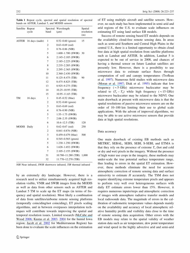
There is usually a trade-off between spatial (i.e., pixel size)

and temporal (i.e., repeat frequency) resolution for satellite

platforms (Table 1). For example, the Landsat 5 has a

repeat cycle of 16 days with 30–120 m spatial resolution

compared with daily coverage of MODIS with 250–

1,000 m. Furthermore, the spatial resolutions of thermal

bands are often coarser than other wavelengths such as

visible, NIR and SWIR (Shortwave-Infrared). For example,

MODIS provides thermal images at 1,000-m resolution

compared with 250-m resolution for images acquired in

other bandwidths on the same satellite platform.

The ET maps derived from remote sensing data acquired

by satellite-based sensors with daily coverage such as

MODIS, geostationary environmental satellite (GOES),

and advanced very high resolution radiometer (AVHRR)

are too coarse to be useful in agricultural regions because

their pixel size is larger than individual fields in most

regions causing significant errors in ET estimation (Tasumi

et al. 2006). The spatial errors in the estimated ET are

partly due to presence of pixels having multiple land uses/

vegetation types with significant differences in cover,

roughness and/or moisture content (Kustas et al. 2004).

This condition is more common in arid and semi-arid

regions where fully irrigated fields are usually surrounded

Irrig Sci (2008) 26:223–237 231

123

by an extremely dry landscape. However, there is a

research need to utilize simultaneously acquired high res-

olution visible, VNIR and SWIR images from the MODIS

as well as data from other sensors such as ASTER and

Landsat 5 TM to scale up the ET maps (in terms of fre-

quency and spatial resolution). Most likely a combination

of data from satellites/airborne remote sensing platforms

(temporally coinciding/not coinciding), ET pixels scaling

algorithms, and in between overpasses interpolation tech-

niques will contribute towards improving the spatial and

temporal resolution issues. Limited research (McCabe and

Wood 2006; Kustas et al. 2003, 2004 for the humid Iowa

region; Jacob et al. 2002 for Mediterranean Region) has

been done to evaluate the scale influences on the estimation

of ET using multiple aircraft and satellite sensors. How-

ever, no such study has been implemented in semi-arid and

arid regions of the U.S. to evaluate scale influences on

estimating ET using land surface EB models.

Success of remote sensing based ET models depends on

the availability cloud-free remote sensing data. In areas

such as semi-arid Southern and Central High Plains in the

central U.S., there is a limited opportunity to obtain cloud

free data at high spatial resolution from satellite platforms

such as Landsat and ASTER. In addition, Landsat 5 is

expected to be out of service in 2008, and chances of

having a thermal sensor on future Landsat satellites are

presently low. However, there is a possibility to use

microwave data to estimate surface fluxes through

computation of soil and canopy temperatures (Trofleau

et al. 1997). Numerous field studies with microwave data

(Moran et al. 1997; Diak et al. 1995) indicate that low

frequency (*5 GHz) microwave backscatter may be

related to (Ts – Ta) while high frequency (*15 GHz)

microwave backscatter may be related to the NDVI. One

main drawback at present with microwave data is that the

spatial resolutions of passive microwave sensors are on the

order of 10–100 km limiting their use to global scale

applications. With the advent of improved algorithms, we

may be able to use active microwave sensors that provide

data at high spatial resolutions.

Data accuracy

One main drawback of existing EB methods such as

METRIC, SEBAL, SEBS, SEBI, S-SEBI, and ETMA is

that they rely on the presence of extreme Ts (hot and cold

or dry and wet) pixels in the imagery. Without the presence

of high water use crops in the imagery, these methods may

under-scale the true potential surface temperature range,

thus leading to errors in the spatial ET estimation. How-

ever, these methods eliminate the need for accurate

atmospheric correction of remote sensing data and surface

emissivity to estimate H accurately. The TSM does not

require identifying extreme temperature pixels and appears

to perform very well over heterogeneous surfaces with

daily ET estimate errors lower than 15%. However, it

requires numerous inputs/steps and atmospheric correction

of images with atmosphere radiative transfer models and

local radiosonde data. The magnitude of errors in the cal-

ibration of radiometric temperature values depends mainly

on the availability and accuracy of local atmospheric rel-

ative humidity profile and visibility data close to the time

of remote sensing data acquisition. Other errors with the

EB models may relate to the spatial validity of weather

station data such as air temperature, dew point temperature

and wind speed in the highly advective arid and semi-arid

Table 1 Repeat cycle, spectral and spatial resolution of spectral

bands on ASTER, Landsat 5, and MODIS sensors

Satellite Repeat

cycle

Spectral

band

Wavelength

(lm)

Spatial

resolution

(m)

ASTER 16 days (nadir) 1 0.52–0.60 (green) 15

2 0.63–0.69 (red)

3 0.76–0.86 (NIR)

5 1.600–1.700 (SWIR) 30

6 2.145–2.185 (SWIR)

7 2.185–2.225 (SWIR)

8 2.235–2.285 (SWIR)

9 2.295–2.365 (SWIR)

10 2.360–2.430 (SWIR)

11 8.125–8.475 (TIR) 90

12 8.475–8.825 (TIR)

13 8.925–9.275 (TIR)

14 10.25–10.95 (TIR)

15 10.95–11.65 (TIR)

TM 16 days 1 0.45–0.52 (blue) 30

2 0.52–0.60 (green)

3 0.63–0.69 (red)

4 0.76–0.90 (NIR)

5 1.55–1.75 (SWIR)

7 2.08–2.35 (SWIR)

6 10.4–12.5 (TIR) 120

MODIS Daily 1 0.62–0.67 (red) 250

2 0.841–0.876 (NIR)

3 0.459–0.479 (blue) 500

4 0.545–0.565 (green)

5 1.230–1.250 (SWIR)

6 1.628–1.652 (SWIR)

7 2.105–2.155 (SWIR)

31 10.780–11.280 (TIR) 1,000

32 11.770–12.270 (TIR)

NIR Near infrared, SWIR shortwave infrared, TIR thermal infrared

232 Irrig Sci (2008) 26:223–237

123

regions as well as the sub-models used to derive LAI, crop

height, fraction cover from remote sensing data.

Data processing time and user friendliness

Timeliness of information products derived from remotely

sensed data remains an unresolved issue since Park et al.

(1968) and others first envisioned remote sensing applica-

tions for agricultural management. This has been revisited

numerous times during the intervening four decades (e.g.,

Jackson 1984; Moran 1994; Moran et al. 1997). To reit-

erate, the usefulness of remote sensing in the estimation of

irrigation water demand will depend on the turn around

time between image acquisition and the dissemination of

derived ET information. At present, the turn around time is

anywhere from 1 to 3 weeks depending on the remote

sensing platform/sensor, algorithm utilized, and techni-

cian’s experience/expertise on applying such algorithms.

However, for most agricultural applications, ET maps

should be delivered within hours, and almost instantaneous

(i.e., real-time) timeliness is required for irrigation sched-

uling. Research should include programs geared towards

rapid processing and analysis of remotely sensed imagery

with the aid of artificial intelligence, to make ET maps

readily available to producers, researchers, and the public

by publishing daily digital ET maps over the Internet.

Review of different ET mapping algorithms presented in

this paper show that most EB models are complex to use.

Literature review indicated that there is an effort towards

the simplification of the procedures to estimate regional ET

mainly through the parameterization of crop coefficients

using vegetation indices or the scaling of potential ET

based on extreme surface temperature pixels. However,

coefficients used in the simplified methods may vary spa-

tially from one region to another. More research needs to

be done in this direction, and some research efforts are

presently underway to address the transferability of crop

coefficients to different location (Howell et al. 2006).

Model validation

Literature review showed that most studies used BR and/or

EC data for development and calibration of regional scale

EB models. It is known that EC method has an energy

balance non-closure problem i.e., Rn = H + LE + G

(Oncley et al. 2000; Twine et al. 2000) of up to 20% even

for non-advective conditions. Measurements of latent heat

flux differed by up to 29% between BR and large, weighing

lysimeters for irrigated alfalfa during advective conditions

in the Southern High Plains of Texas (Todd et al. 2000).

Therefore, calibration of the EB models against lysimetric

and/or well-calibrated scintillometer measurements over

irrigated and dryland conditions may enhance their ability

to estimate regional ET accurately. In addition, heat flux

source models should be utilized to properly weight and

integrate LE pixels, for example, upwind of BR, EC, and/or

scintillometer stations in the process of comparison of LE

estimates with measured values (Chavez et al. 2005).

Conclusions

Reliable regional ET estimates are essential to improve

spatial crop water management. Land surface EB models,

using remote sensing data from ground to airborne to

satellite platforms at different spatial resolutions, have

been found to be promising for mapping daily and sea-

sonal ET at a regional scale. In this paper, a thorough

review of numerous remote sensing based models was

made to understand the current status of the regional ET

research, underlying principle for each method, data

requirements, and their strengths and weaknesses. In all

EB methods, thermal remote sensing data is one of the

crucial inputs. In general, ET estimation errors associated

with EB models were mostly found in the range of 2.7–

35% for daily ET and less than 6% for seasonal ET, with

larger errors associated with simplified methods. Reflec-

tance based crop coefficient methods are relatively easy to

use to estimate ET compared to EB models, however,

crop coefficients must account for water stress and require

calibration for each crop type. Further, a major limitation

of this approach is the spatial validity of the estimated

reference ET.

Although the remote sensing based ET models shown to

have the potential to accurately estimate regional ET, there

are opportunities to further improve these models through

(1) developing methods for accurately estimating canopy

temperature profiles, (2) testing the spatial validity of the

meteorological data such as air temperature and wind speed

used in the EB models, and (3) testing the sub-models used

to estimate soil heat flux, LAI, crop height, etc., for their

accuracy, under various agrometeorological/environmental

conditions. In addition, further evaluation of different

scaling methods to extrapolate remote sensing derived

instantaneous ET to daily and seasonal ET values is

needed.

The spatial and temporal remote sensing data from

existing set of earth observing satellite sensors are not

sufficient to use their ET products for irrigation scheduling.

This may be constrained further by the disappearance of

thermal sensors on future Landsat satellites. However,

research opportunities exist to improve the spatial and

temporal resolution of ET by developing algorithms similar

to those by McCabe and Wood (2006), Kustas et al. (2003),

Irrig Sci (2008) 26:223–237 233

123

Norman et al. (2003), Kustas et al. (2004), or Jacob et al.

(2002) to improve spatial resolution of reflectance and

surface temperature data derived from Landsat/ASTER/

MODIS images using same/other-sensor high resolution

visible, NIR and SWIR images. Finally, weighting and

integrating remote sensing derived ET pixels should be

done using footprint (heat flux source area) models for

proper comparison to measured values by EC, BR or

scintillometer energy balance stations.

References

Allen R, Pereira L, Raes D, Smith M (1998) Crop evapotranspiration:

guidelines for computing crop water requirements. FAO Irriga-

tion and Drainage Paper No. 56. FAO, Rome

Allen RG, Tasumi M, Trezza R (2002) METRICTM: mapping

evapotranspiration at high resolution—application manual for

Landsat satellite imagery. University of Idaho, Kimberly

Allen RG, Tasumi M, Morse A (2005) Satellite-based evapotranspi-

ration by METRIC and Landsat for western states water

management. US Bureau of Reclamation Evapotranspiration

Workshop, Feb 8–10, 2005, Ft. Collins

Allen RG, Tasumi M, Trezza R (2007a) Satellite-based energy

balance for mapping evapotranspiration with internalized cali-

bration (METRIC)-Model. ASCE J Irrigation Drainage Eng (in

press)

Allen RG, Tasumi M, Morse A, Trezza R, Wright JL, Bastiaanssen

W, Kramber W, Lorite-Torres I, Robison CW (2007b) Satellite-

based energy balance for mapping evapotranspiration with

internalized calibration (METRIC)-applications. ASCE J Irriga-

tion Drainage Eng (in press)

Alves I, Fontes JC, Pereira LS (2000) Evapotranspiration estimation

from infrared surface temperature. I: Performance of the flux

equation. Trans ASAE 43(3):591–598

Anderson CM, Kustas WP, Norman JM (2007) Upscaling flux

observations from local to continental scales using thermal

remote sensing. Agron J 99:240–254

Bartholic JF, Namken LN, Wiegand CL (1972) Aerial thermal

scanner to determine temperatues of soils and of crop canopies

differing in water stress. Agron J 64:603–608

Bastiaanssen WGM (1995) Regionalization of surface flux densities

and moisture indicators in composite terrain: a remote sensing

approach under clear skies in Mediterranean climates. PhD

Dissertation, CIP Data Koninklijke Blibliotheek, Den Haag, The

Netherlands

Bastiaanssen WGM, Menenti M, Feddes RA, Holtslang AA (1998) A

remote sensing surface energy balance algorithm for land

(SEBAL): 1. Formulation. J Hydrol 212–213:198–212

Bastiaanssen WGM, Noordman EJM, Pelgrum H, Davids G, Thore-

son BP, Allen RG (2005) SEBAL model with remotely sensed

data to improve water-resources management under actual field

conditions. ASCE J Irrigation Drainage Eng 131(1):85–93

Bausch WC (1993) Soil background effects on reflectance-based crop

coefficients for corn. Remote Sensing Environ 46:213–222

Bausch WC, Neale CMU (1987) Crop coefficients derived from

reflectance canopy radiation: a concept. Trans ASAE 30(3):703–

709

Brest CL, Goward SN (1987) Driving surface albedo measurements

from narrow band satellite data. Int J Remote Sensing 8:351–367

Brown KW (1974) Calculations of evapotranspiration from crop

surface temperature. Department of Soil and Crop Science,

College Station

Brown KW, Rosenberg NJ (1973) A resistance model to predict

evapotranspiration and its application to a sugar beet field. Agron

J 68:635–641

Brunsell NA, Gillies R (2002) Incorporating surface emissivity into a

thermal atmospheric correction. Photogrammetric Eng Remote

Sensing J 68(12):1263–1269

Brutsaert W (1975) On a derivable formula for long-wave radiation

from clear skies. Water Resources Res 11:742–744

Brutsaert W (1999) Aspect of bulk atmospheric boundary layer

similarity under free-convective conditions. Rev Geophys

37:439–451

Brutsaert W, Sugita M (1992) Application of self-preservation in the

diurnal evolution of the surface energy budget to determine daily

evaporation. J Geophys Res 97:18377–18382

Chavez JL, Neale CMU (2003) Validating airborne multispectral

remotely sensed heat fluxes with ground energy balance tower

and heat flux source area (footprint) functions. ASAE Paper No.

033128. St. Joseph, Michigan

Chavez JL, Neale CMU, Hipps LE, Prueger JH, Kustas WP (2005)

Comparing aircraft-based remotely sensed energy balance fluxes

with eddy covariance tower data using heat flux source area

functions. J Hydrometeorol AMS 6(6):923–940

Chavez JL, Neale CMU (2007) Daily evapotranspiration estimates

from airborne remote sensing and ground data inputs. Trans

ASABE (submitted)

Chavez JL, Gowda PH, Evett SR, Colaizzi PD, Howell TA, Marek T

(2007) An application of METRIC for ET mapping in the Texas

high plains. Trans ASABE (submitted)

Chehbouni A, Lo Seen D, Njoku EG, Monteny B (1996) Examination

of the difference between radiative and aerodynamic surface

temperatures over sparsely vegetated surfaces. Remote Sensing

Environ 58:177–186

Chehbouni A, Nouvellon Y, Lhomme J-P, Watts C, Boulet G, Kerr

YH, Moran MS, Goodrich DC (2001) Estimation of surface

sensible heat flux using dual angle observations of radiative

surface temperature. J Agric Forest Meteorol 108:55–65

Choudhury FJ, Idso SB, Reginato RJ (1987) Analysis of an empirical

model for soil heat flux under a growing wheat crop for

estimating evaporation by an infrared-temperature based energy

balance equation. Agric Forest Meteorol 39:283–297

Colaizzi PD, Evett SR, Howell TA, Tolk JA (2004) Comparison of

aerodynamic and radiometric surface temperature using preci-

sion weighing lysimeters. In: Gao W, Shaw DR (eds)

Proceedings of SPIE 49th annual meeting, remote sensing and

modeling of ecosystems for sustainability, vol 5544, pp 215–229

Colaizzi PD, Evett SR, Howell TA, Tolk JA (2006a) Comparison of

five models to scale daily evapotranspiration from one-time-of-

day measurements. Trans ASABE 49(5):1409–1417

Colaizzi PD, Evett SR, Howell TA, Tolk JA, Li F (2006b) Evaluation

of a two-source balance model in an advective environment.

Proc. World Enviromental and Water Resources Congress. May

21–24, 2006. Omaha, NE. EWRI, ASCE (CD-ROM)

Crago RD (2000) Conservation and variability of the evaporative

fraction during the daytime. J Hydrol 180(1–4):173–194

Crago R, Friedl M, Kustas W, Wang Y (2004) Investigation of

aerodynamic and radiometric land surface temperatures. NASA

Scientific and Technical Aerospace Reports (STAR) 42(1)

Diak GR, Rabin RM, Gallo KP, Neale CM (1995) Regional scale

comparisons of NDVI, soil moisture indices from surface and

microwave data and surface energy budgets evaluated from

satellite and in-situ data. Remote Sensing Rev 12:355–382

D’Urso G, Santini A (1996) A remote sensing and modeling

integrated approach for the management of irrigation distribution

systems. In: Proceedings of the international conference on

‘‘Evapotranspiration and Irrigation Scheduling’’, San Antonio

(USA), vol 4–6, pp 435–441

234 Irrig Sci (2008) 26:223–237

123

Er-Raki S, Chehbouni A, Guemouria N, Duchemin B, Ezzahar J,

Hadria R (2007) Combining FAO-56 model and ground-based

remote sensing to estimate water consumptions of wheat crops in

a semi-arid region. Agric Water Manage 87:41–54

Gomez M, Olioso A, Sobrino JA, Jacob F (2005) Retrieval of

evapotranspiration over the Alpille/ReSeDA experimental site

using airborne POLDER sensor and a thermal camera. Remote

Sensing Environ 96:399–408

Gonzalez-Dugo MP, Neale CMU, Mateos L, Kustas WP, Li F (2006)

Comparison of remotely sensing-based energy balance methods

for estimating crop evapotranspiration. In: Owe M, D’Urso G,

Christopher Neale MU, Gouweleeuw BT (eds) Proceeding of

SPIE, vol 6359: remote sensing for agriculture, ecosystems, and

hydrology VIII, p 6359Z

Hanson RL (1991) Evapotranspiration and droughts. In: Paulson RW,

Chase EB, Roberts RS, Moody DW, Compilers, National

Water Summary 1988-89-hydrologic events and floods and

droughts: U.S. Geological Survey Water-Supply Paper 2375,

pp 99–104

Harikishan J, Neale CMU, Wright JL (2006) Development and

validation of canopy reflectance based crop coefficient for

potato. Agric Water Manage (in press)

Hatfield JL, Perrier A, Jackson RD (1983) Estimation of evapotrans-

piration at on time-of-day using remotely sensed surface

temperatures. Agric Water Manage 7:341–350

Hatfield JL, Reginato RJ, Idso SB (1984) Evaluation of canopy

temperature-evapotranspiration model over various crops. Agric

Forest Meteorol 32:41–53

Heilman JL, Kanemasu ET, Rosenberg NJ, Blad BL (1976) Thermal

scanner measurements of canopy temperatures to estimate

evapotranspiration. Remote Sensing Environ 5:137–145

Heilman JL, Heilman WE, Moore DG (1982) Evaluating the crop

coefficient using spectral reflectance. Agron J 74:967–971

Hipps LE (1989) The infrared emissivities of soil and Artemisia

tridentate and subsequent temperature corrections in a shrub-

steppe ecosystem. Remote Sensing Environ 27:337–342

Howell TA, Evett SR, Tolk JA, Copeland KS, Dusek DA, Colaizzi

PD (2006) Crop coefficients developed at Bushland, Texas for

corn, wheat, sorghum, soybean, cotton, and alfalfa. In: Proceed-

ings of 2006 ASCE-EWRI World Water and Environmental

Resources Congress, 21–25 May, Omaha

Huete A (1988) A soil adjusted vegetation index (SAVI). Remote

Sensing Environ 25:295–309

Hunsaker DJ, Barnes EM, Clarke TR, Fitzgerald GJ, Pinter PJ Jr

(2005) Cotton irrigation scheduling using remotely sensed and

FAO-56 basal crop coefficients. Trans ASAE 48(4):1395–1407

Idso SB, Schmugge TJ, Jackson RD, Raginato RJ (1975) The utility

of surface temperature measurements for the remote sensing of

the soil water status. J Geophys Res 80:3044–3049

Jackson RD (1984) Remote sensing of vegetation characteristics for

farm management. SPIE 475:81–96

Jackson RD, Reginato RJ, Idso SB (1977) Wheat canopy temperature:

a practical tool for evaluating water requirements. Water Resour

Res 13:651–656

Jackson RD, Idso SB, Reginato RJ, Pinter PJ (1980) Remotely sensed

crop temperatures and reflectances as inputs to irrigation

scheduling. In: Proceedings of American Society of Civil

Engineers, Irrigation and Drainage Division, Specialty Confer-

ence, Boise, Idaho, pp 390–397

Jackson RD, Idso SB, Reginato RJ, Pinter PJ Jr (1981) Canopy

temperature as a crop water stress indicator. Water Resour Res

17(4):1133–1138

Jackson RD, Hatfield JL, Reginato RJ, Idso SB, Pinter PJ Jr (1983)

Estimation of daily evapotranspiration from one time-of-day

measurements. Agric Water Manage 7:351–362

Jackson RD, Pinter PJ Jr, Reginato RJ (1985) Net radiation calculated

from remote and multispectral and ground station meteorological

data. Agric Forest Meteorol 35:153–164

Jackson RD, Moran MS, Gay LW, Raymond LH (1987) Evaluating

evaporation from field crops using airborne radiometry and

ground-based meteorological data. Irrigation Sci 8:81–90

Jacob F, Olioso A, Gu XF, Su A, Seguin B (2002) Mapping surface

fluxes using airborn visible, near infrared remote sensing data

and a spatialized surface energy balance model. Agronomie

22:669–680

Kalma JD, Jupp DLB (1990) Estimating evaporation from pasture

using infrared thermometry: evaluation of a one-layer resistance

model. Agric Forest Meteorol 51:223–246

Kanemasu ET, Stone LR, Powers WL (1977) Evapotranspiration

model tested for soybeans and sorghum. Agron J 68:569–572

Kimes DS (1980) Effects of vegetation canopy structure on remotely

sensed canopy temperatures. Remote Sensing Environ 10:165–

174

Kimes DS (1983) Dynamics of directional reflectance factor distri-

butions for vegetation canopies. Appl Opt 22(9):1364–1372

Kimes DS, Smith JA, Ranson KJ (1980) Vegetation reflectance

measurements as a function of solar zenith angle. Photogram-

metric Eng Remote Sensing 46:1563–1573

Kustas WP, Daughtry CST (1990) Estimation of the soil heat flux/net

radiation ratio from multispectral data. Agric Forest Meteorol

49:205–223

Kustas WP, Norman JM (1996) Use of remote sensing for

evapotranspiration monitoring over land surfaces. Hydrol Sci J

41(4):495–516

Kustas WP, Norman JM (1999) Evaluation of soil and vegetation heat

flux predictions using a simple two-source model with radio-

metric temperatures for partial canopy cover. Agric Forest

Meteorol 94:13–29

Kustas WP, Choudhury BJ, Moran MS, Reginato RJ, Jackson RD,

Gay LW, Weaver HL (1989) Determination of sensible heat flux

over sparse canopy using thermal infrared data. Agric Forest

Meteorol 44:197–216

Kustas WP, French AN, Hatfield JL, Jackson TJ, Moran MS, Rango

A, Ritchie JC, Schumgge TJ (2003) Remote sensing research in

Hydrometeorology. Photogrammetric Eng Remote Sensing

69(6):631–646

Kustas WP, Li F, Jackson TJ, Prueger JH, MacPherson JI, Wolde M

(2004) Effects of remote sensing pixel resolution on modeled

energy flux variability of croplands in Iowa. Remote Sensing

Environ 92:535–547

Kustas WP, Anderson MA, Norman JM, Li F (2007) Utility of

radiometric-aerodynamic temperature relations for heat flux

estimation. Boundary-Layer Meteorol 122:167–187

Loheide II SP, Gorelick SM (2005) A local-scale, high resolution

evapotranspiration mapping algorithm (ETMA) with hydroeco-

logical applications at riparian meadow restoration sites. Remote

Sensing Environ 98:182–200

Matsushima D (2000) An estimation method for regional sensible

heat flux on vegetation using satellite infrared temperature. In:

Proceedings of the 15th conference of hydrology/80th AMS

annual meeting, P1.29. Long Beach

Matsushima D (2005) Relations between aerodynamic parameters and

heat transfer and thermal-infrared thermometry in the bulk

surface formulation. J Meteorol Soc Jpn 83(3):373–389

McCabe MF, Wood EF (2006) Scale influences on the remote

estimation of evapotranspiration using multiple satellite sensors.

Remote Sensing Environ 105:271–285

Menenti M, Choudhury BJ (1993) Parameterization of land surface

evapotranspiration using a location dependent potential evapo-

transpiration and surface temperature range. In: Bolle HJ et al

Irrig Sci (2008) 26:223–237 235

123

(eds) Proceedings of exchange processes at the land surface for a

range of space and time scales. IAHS Publ 212, pp 561–568

Menenti M, Jia L, Su Z (2003) On SEBI-SEBS validation in France,

Intaly, Spain, USA and China. In: Co-Chair Allen RG,

Bastiaanssen W (eds) Proceedings of the workshop on use of

remote sensing of crop evapotranspiration for large regions.

International Commission on Irrigation and Drainage (ICID),

Montpellier

Micheal MG, Bastiaanssen WGM (2000) A new simple method to

determine crop coefficients for water allocation planning from

satellites: results from Kenya. Irrigation Drainage Syst 14:237–

256

Monteith JL (1965) Evaporation and environment. Symp Soc Explor

Biol 19:205–234

Monteith JL (1981) Evaporation and surface temperature. Quart J R

Meteorol Soc 107:1–27

Moran MS (1994) Irrigation management in Arizona using satellites

and airplanes. Irrigation Sci 15(1):35–44

Moran MS, Jackson RD, Raymond LH, Gay LW, Slater PN (1989)

Mapping surface energy balance components by combining

Landsat Thematic Mapper and ground-based meteorological

data. Remote Sensing Environ 30:77–87

Moran MS, Vidal A, Troufleau D, Qi J, Clarke TR, Pinter PJ Jr,

Mitchell TA, Inoue Y, Neale CMU (1997) Combining multifre-

quency microwave and optical data for crop management.

Remote Sensing Environ 61:96–109

Neale CMU, Bausch WC, Heeremann DF (1989) Development of

reflectance-based crop coefficients for corn. Trans ASAE

32(6):1891–1899

Neale CMU, Ahmed RH, Moran MS, Pinter PJ, Qi J, Clarke TR

(1996) Estimating seasonal cotton evapotranspiration using

canopy reflectance. In: Camp CR, Sadler EJ, Yoder RE (eds)

Evapotranspiration and irrigation scheduling: proceedings of the

international conference, November 3–6, 1996. San Antonio. St.

Joseph, Michigan, pp 173–181

Neale CMU, Jayanthi H, Wright JL (2003) Crop and irrigation water

management using high resolution airborne remote sensing. In:

Proceedings of 54th IEC meeting of the international commis-

sion on irrigation and drainage (ICID) workshop remote sensing

of ET for large regions, 17 Sept (2003) Montpellier, France.

CD-ROM. New Delhi, India

Norman JM, Becker F (1995) Terminology in thermal infrared remote

sensing of natural surfaces. Agric For Meteorol 77:153–166

Norman JM, Kustas WP, Humes KS (1995) A two-source approach

for estimating soil and vegetation energy fluxes from observa-

tions of directional radiometric surface temperature. Agric For

Meteorol 77:263–293

Norman JM, Kustas WP, Prueger JH, Diak GR (2000a) Surface flux

estimation using radiometric temperature: a dual temperature

difference method to minimize measurement error. Water

Resour Res 36:2263–2274

Norman JM, Kustas WP, Prueger JH, Diak GR (2000b) Surface flux

estimation using radiometric temperature: dual-temperature-

difference method to minimize measurement errors. Water

Resour Res 36(8):2263–2274

Norman JM, Anderson MC, Kustas WP, French AN, Mecikalski J,

Torn R, Diak GR, Schmugge TJ, Tanner BCW (2003) Remote

sensing of surface energy fluxes at 101-m pixel resolutions.

Water Resour Res 39(8):1221

Oncley SP, Foken T, Vogt R, Bernhofer C, Liu H, Sorbjan Z Pitacco

A, Grantz D, Ribeiro L (2000) The EBEX 2000 field experiment.

In: 14th Symposium on boundary layers and turbulence, Aspen.

American Meteorological Society, Boston, pp 322–324

Park AB, Colwell RN, Meyers VF (1968) Resource survey by

satellite; science fiction coming true. Yearbook of Agriculture,

pp 13–19

Price JC (1982) Estimation of regional scale evapotranspiration

through analysis of satellite thermal-infrared data. IEEE Trans

Geosci Remote Sens GE-20:286–292

Reginato RJ, Jackson RD, Pinter PJ Jr (1985) Evapotranspiration

calculated from remote multi-spectral and ground station mete-

orological data. Remote Sensing Environ 18:75–89

Roerink GJ, Su B, Menenti M (2000) S-SEBI A simple remote

sensing algorithm to estimate the surface energy balance. Phys

Clim Earth (B) 25(2):147–157

Rosenberg NJ, Blad BL, Verma SB (1983) Microclimate, the

biological environment, 2nd edn. Wiley, New York, 495p

Rouse JW, Haas RH Jr, Schell JA, Deering DW (1974) Monitoring

vegetation systems in the Great Plains with ERTS. In: Proceed-

ings of the ERTS-1 3rd Symposium, vol 1. NASA SP-351.

NASA, Washington, pp 309–317

Seguin B, Itier B (1983) Using midday surface temperature to

estimate daily evapotranspiration from satellite thermal data IR.

Int J Remote Sensing 4(2):371–383

Sellers PJ, Randall DA, Collatz GJ, Berry JA, Field CB, Dazlich DA,

Zhang C, Collelo GD, Nounoua L (1996) A revised land surface

parameterization (SiB2) for atmospheric GCMS, Part 1: Model

formulation. J Clim 9:676–705

Shuttleworth WJ, Gurney RJ (1990) The theoretical relationship

between foliage temperature and canopy resistance in sparse

crops. Quart J R Meteorol Soc 116:497–519

Shuttleworth WJ, Wallace JS (1985) Evaporation from sparse crops—

an energy combination theory. Quart J Roy Meteorol Soc

111:839–855

Stone LR, Horton ML (1974) Estimating evapotranspiration using

canopy temperatures: field evaluation. Agron J 66:450–454

Su Z (2002) The surface energy balance system (SEBS) for

estimation of turbulent fluxes. Hydrol Earth Syst Sci 6:85–99

Su Z, Schmugge T, Kustas WP, Massman WJ (2001) An evaluation

of two models for estimation of the roughness height for heat

transfer between the land surface and the atmosphere. J Appl

Meteorol 40:1933–1951

Su H, McCabe MF, Wood EF, Su Z, Prueger JH (2005) Modeling

evapotranspiration during SMACEX: comparing two approaches

local- and regional-scale prediction. J Hydrometerol 6(6):910–

922

Taconet O, Bernard R, Vidal-Madjar D (1986) Evapotranspiration

over an agricultural region using a surface flux/temperature

model based on NOAA-AVHRR data. J Clim Appl Meteorol

25:284–307

Tasumi M, Trezza R, Allen RG, Wright JL (2003) U.S. Validation

tests on the SEBAL model for evapotranspiration via satellite.

In: Proceedings of 54th IEC meeting of the international

commission on irrigation and drainage (ICID) Workshop remote

sensing of ET for large regions, 17 Sept (2003) Montpellier,

France

Tasumi M, Trezza R, Allen RG, Wright JL (2005a) Operational

aspects of satellite-based energy balance models for irrigated

crops in the semi-arid U.S. J Irrigation Drainage Syst 19:355–

376

Tasumi M, Allen RG, Trezza R, Wright JL (2005b) Satellite-based

energy balance to assess within-population variance of crop

coefficient curves. ASCE J Irrigation Drainage Eng 131(1):94–

109

Tasumi M, Allen RG, Trezza R (2006) Calibrating satellite-based

vegetation indices to estimate evapotranspiration and crop

coefficients. In: Wichelns D, Anderson SS (eds) Proceedings

of the 2006 USCID Water Management Conference. Ground

water and surface water under stress: competition, interaction,

solutions. Publisher USCID, Denver

Todd RW, Evett SR, Howell TA (2000) The Bowen ratio-energy

balance method for estimating latent heat flux of irrigated alfalfa

236 Irrig Sci (2008) 26:223–237

123

evaluated in a semi-arid, advective environment. Agric Forest

Meteorol 103:335–348

Trezza R (2002) Evapotranspiration using a satellite-based surface

energy balance with standardized ground control. PhD Disser-

ation, Biological and Irrigation Engineering Department, Utah

State University, Logan

Trofleau D, Vidal A, Beaudon A, Moran MS, Weltz MA, Goodrich

DC, Washburne J, Rahman AF (1997) Optical-microwave

synergy for estimating surface sensible heat flux over a semi-

arid rangeland. Remote Sensing Rev 15:113–132

Twine TE, Kustas WP, Norman JM, Cook DR, Houser PR, Meyers

TP, Prueger JH, Starks PJ, Wesley ML (2000) Correcting eddy-

covariance flux underestimates over grassland. Agric Forest

Meteorol 103:279–300

Verma SB, Rosenberg NJ, Blad BL, Baradas MW (1976) Resistance-

energy balance method for predicting evapotranspiration: deter-

mination of boundary layer resistance and evaluation of error

effects. Agron J 68:776–782

Zibognon M, Crago R, Suleiman A (2002) Conversion of radiometric

to aerodynamic surface temperature with an anishothermal

canopy model. Water Resour Res 38(6):1067

Zhang L, Lemeur R (1995) Evaluation of daily ET estimates from

instantaneous measurements. Agric Forest Meteorol 74:139–154

Zhang Y, Wegehenkel M (2006) Integration of MODIS data into a

single model for the spatial distributed simulation of soil water

content and evapotranspiration. Remote Sensing Environ

104:393–408

Irrig Sci (2008) 26:223–237 237

123