1318 IEEE TRANSACTIONS ON ANTENNAS AND PROPAGATION, VOL. 54, NO. 4, APRIL 2006

Estimation of Radio Refractivity From Radar ClutterUsing Bayesian Monte Carlo Analysis

Caglar Yardim, Student Member, IEEE, Peter Gerstoft, and William S. Hodgkiss, Member, IEEE

Abstract—This paper describes a Markov chain Monte Carlo(MCMC) sampling approach for the estimation of not only theradio refractivity profiles from radar clutter but also the uncertain-ties in these estimates. This is done by treating the refractivity fromclutter (RFC) problem in a Bayesian framework. It uses unbiasedMCMC sampling techniques, such as Metropolis and Gibbs sam-pling algorithms, to gather more accurate information about theuncertainties. Application of these sampling techniques using anelectromagnetic split-step fast Fourier transform parabolic equa-tion propagation model within a Bayesian inversion frameworkcan provide accurate posterior probability distributions of the es-timated refractivity parameters. Then these distributions can beused to estimate the uncertainties in the parameters of interest.Two different MCMC samplers (Metropolis and Gibbs) are ana-lyzed and the results compared not only with the exhaustive searchresults but also with the genetic algorithm results and helicopter re-fractivity profile measurements. Although it is slower than globaloptimizers, the probability densities obtained by this method arecloser to the true distributions.

Index Terms—Atmospheric ducts, genetic algorithms, Markovchain Monte Carlo (MCMC) techniques, radar clutter, refractivityestimation.

I. INTRODUCTION

AN accurate knowledge of radio refractivity is essential inmany radar and propagation applications. Especially at

low altitudes, radio refractivity can vary considerably with bothheight and range, heavily affecting the propagation characteris-tics. One important example is the formation of an electromag-netic duct. A signal sent from a surface or low altitude source,such as a ship or low-flying object, can be totally trapped insidethe duct. This will result in multiple reflections from the surfaceand they will appear as clutter rings in the radar plan positionindicator (PPI) screen (Fig. 1). In such cases, a standard atmo-spheric assumption with a slope of modified refractivity of 0.118M-units/m may not give reliable predictions for a radar systemoperating in such an environment.

Ducting is a phenomenon that is encountered mostly insea-borne applications due to the abrupt changes in the ver-tical temperature and humidity profiles just above large water

Manuscript received May 18, 2005; revised October 10, 2005. This work wassupported by the Office of Naval Research Code 32 under Grant N00014-05-1-0369.

C. Yardim and W. S. Hodgkiss are with the Electrical and Computer Engi-neering Department, University of California, San Diego, La Jolla, CA 92093USA and also with the Marine Physical Laboratory, Scripps Institution ofOceanography, University of California, San Diego, La Jolla, CA 92093 USA(e-mail: cyardim@ucsd.edu, whodgkiss@ucsd.edu).

P. Gerstoft is with the Marine Physical Laboratory, Scripps Institution ofOceanography, University of California, San Diego, La Jolla, CA 92093 USA(e-mail: gerstoft@ucsd.edu)

Digital Object Identifier 10.1109/TAP.2006.872673

Fig. 1. Clutter map from Space Range Radar (SPANDAR) at Wallops Island,VA.

Fig. 2. Trilinear M-profile and its corresponding coverage diagram.

masses, which may result in an sharp decrease in the modifiedrefractivity (M-profile) with increasing altitude. This will,in turn, cause the electromagnetic signal to bend downward,effectively trapping the signal within the duct. It is frequentlyencountered in many regions of the world such as the PersianGulf, the Mediterranean, and California. In many cases, asimple trilinear M-profile is used to describe this variation. Thecoverage diagram of a trapped signal in such an environment isgiven in Fig. 2.

The first attempt in estimating the M-profile from radar clutterreturns using a maximum likelihood (ML) approach was madein [1] and was followed by similar studies, which used either amarching-algorithm approach [2] or the global-parametrizationapproach [3], [4]. The latter is adopted in this paper. The main

0018-926X/$20.00 © 2006 IEEE

YARDIM et al.: ESTIMATION OF RADIO REFRACTIVITY FROM RADAR CLUTTER 1319

Fig. 3. The four-parameter trilinear M-profile model used in this work.

purpose of these studies is to estimate the M-profile using onlythe radar clutter return, which can readily be obtained duringthe normal radar operation, without requiring any additionalmeasurements or hardware. A near-real-time estimation can beachievedwithasufficientlyfastoptimizer.Moreover,informationobtained from other sources can be easily incorporated intothe Bayesian formulation, e.g., the statistics of M-profiles inthe region, meteorological model simulation results, helicopter,radiosonde, or some other ship-launched in situ instrumentmeasurements.

To address the uncertainties in the M-profile parameter esti-mates, determination of the basic quantities such as the mean,variance, and marginal posterior probability distribution of eachestimated parameter is necessary. They can be computed bytaking multidimensional integrals of the posterior probabilitydensity (PPD), which can be accomplished by a Markov chainMonte Carlo (MCMC) sampling method within a Bayesian in-version structure. MCMC is selected because it provides unbi-ased sampling of the PPD, unlike global optimizers such as thegenetic algorithm, which usually oversample the peaks of thePPD and introduce a bias [5].

Bayesian inversion is a likelihood-based technique which,when combined with a powerful sampling algorithm such asMCMC, can be an effective tool in the estimation of uncertaintyin nonlinear inversion problems such as the electromagnetic re-fractivity from clutter (RFC) inversion. An alternative approach,which does not make use of likelihood, is given in [6]. The like-lihood formulations are based on those used in [7]. The MCMCsampler employs a split-step fast Fourier transform (FFT) para-bolic equation code as its forward propagation model.

II. THEORY

The M-profile is assumed range-independent, and a simpletrilinear profile is used to model the vertical M-profile (Fig. 3).An M-profile with parameters is represented by the vector

, with the element being the value of the th parameter.Each of these environmental parameters is then treated as anunknown random variable. Therefore, an -dimensional jointposterior PPD can be defined using all of the parameters. All of

TABLE INOTATION

the desired quantities such as the means, variances, and marginalposterior distributions can be found using the PPD. A summaryof the notation used is given in Table I.

The -parameter refractivity model is given to a forwardmodel, an electromagnetic split-step FFT parabolic equation,along with the other necessary input parameters such as fre-quency, transmitter height, beamwidth, and antenna beampattern [8], [9]. The forward model propagates the field in amedium characterized by and outputs the radar clutter .This is then compared with the measured clutter data , and anerror function is derived for the likelihood function. Inprevious global-parametrization approaches, this error functionwas used by a global optimization algorithm such as the geneticalgorithm (GA), which would minimize and reach theML solution. Instead of GA, a likelihood function based on

can be used in a Metropolis or Gibbs sampler. Thismakes it possible to get not only the ML solution but also betterestimates for the uncertainties in terms of variances, marginaland multidimensional PPDs.

A. Bayesian Inversion

RFC can be solved using a Bayesian framework, where theunknown environmental parameters are taken as random vari-ables with corresponding one-dimensional (1-D) probabilitydensity functions (pdfs) and an -dimensional joint pdf. Thisprobability function can be defined as the probability of themodel vector given the experimental data vector ,and it is called the posterior pdf (PPD). with the highestprobability is referred to as the maximum a posteriori (MAP)solution. For complex probabilities, global optimizers such asthe genetic algorithm or simulated annealing can be used tofind the MAP solution. An alternative to this is minimizing the

1320 IEEE TRANSACTIONS ON ANTENNAS AND PROPAGATION, VOL. 54, NO. 4, APRIL 2006

mean square error between clutter data and the reconstructedclutter . It is referred to as the Bayesian minimum meansquare error estimator and can easily be shown to be equal tothe vector mean of [10]. Both estimates are calculatedin this paper. Due to the fact that a noninformative prior is used,MAP and ML solutions are the same and will be referred tosimply as ML from now on. The posterior means, variances,and marginal probability distributions then can be found bytaking - or ( 1)-dimensional integrals of this PPD

(1)

(2)

(3)

Posterior density of any specific environmental parameter suchas the M-deficit or the duct height can be obtained by marginal-izing the -dimensional PPD as given in (3). Joint probabilitydistributions can be obtained using similar integrations. For fur-ther details about Bayesian inverse theory, see [10] and [11].

The posterior probability can be found using Bayes’ formula

(4)

with

(5)

The likelihood function will be defined in the next sec-tion. The prior represents the a priori knowledge aboutthe environmental parameters before the experiment. There-fore, it is independent of the experimental results and, hence, .The evidence appears in the denominator of the Bayes’ formulaas . It is the normalizing factor for and is indepen-dent of the parameter vector . A noninformative or flat priorassumption will reduce (4) to

(6)

B. Likelihood Function

Assuming a zero-mean Gaussian-distributed error, the likeli-hood function can be written as

(7)

where is the data covariance matrix, is the transpose,and is the number of range bins used (length of the datavector ). Further simplification can be achieved by assumingthat the errors are spatially uncorrelated with identical distri-bution for each data point forming the vector . For this case,

, where is the variance and the identity matrix.Defining an error function by

(8)

the likelihood function can be written as

(9)

Therefore, recalling (6), the posterior probability density can beexpressed as

(10)

The calculation of probabilities of all possible combinationsalong a predetermined grid is known as the exhaustive searchand practically can be used for up to four to five parameters,depending on the forward modeling CPU speed. However, as

increases further, it becomes impractical. Therefore, there isa need for an effective technique that can more efficiently esti-mate not only the posterior probability distribution but also themultidimensional integrals given in (1)–(3).

C. Markov Chain Monte Carlo Sampling

MCMC algorithms are mathematically proven to sample the-dimensional state space in such a way that the PPD obtained

using these samples will asymptotically be convergent to thetrue probability distribution. There are various implementationsof MCMC such as the famous Metropolis–Hastings (or simpli-fied Metropolis version) algorithm, which was first introducedin [12], and Gibbs sampling, which was made popular amongthe image processing community by [13]. They are extensivelyused in many other fields such as geophysics [11] and oceanacoustics [5], [14], [15].

To have asymptotic convergence in the PPD, a Markov chainsampler must satisfy the detailed balance [16]. Markov chainswith this property are also called reversible Markov chains, andit guarantees the chain to have a stationary distribution. MCMCsamplers satisfy this detailed balance. Moreover, we can setup the MCMC such that the desired distribution (PPD) is thestationary distribution. Hence, the sample distribution willconverge to the PPD as more and more samples are collected.Global optimizers do not satisfy detailed balance, and theyusually oversample the high probability regions since theyare designed as point estimators, trying to get to the optimalsolution point fast, not to wander around the state space tosample the distribution. On the contrary, an unbiased samplerfollowing MCMC rules will spend just enough time on lowerprobability regions and the histogram formed from the sampleswill converge to the true distribution.

Metropolis and Gibbs samplers are selected as theMCMC algorithms to be used here. The working prin-ciple for both methods is similar. Assume the th sampleis . In the -dimensional parameterspace, new MCMC samples are obtained by drawing from

YARDIM et al.: ESTIMATION OF RADIO REFRACTIVITY FROM RADAR CLUTTER 1321

successive 1-D densities. Selection of the next MCMCsample starts with fixing allcoordinates except the first one. Then the intermediate point

is selected by drawing a random value froma one-dimensional distribution around . The new point

is then used as the starting point to updatethe second parameter by drawing a value for . The nextsample is formed when all the parameters are updatedonce successively. The difference between the two methods liesin the selection of the 1-D distributions.

1) Metropolis Algorithm: In the more generalMetropolis–Hastings algorithm, the 1-D distribution can beany distribution. However, in the simplified version, called theMetropolis algorithm, the 1-D distribution has to be symmetric.The most common ones used in practice are the uniform andGaussian distributions (a variance of 0.2 search interval isused) centered around the . Likelihood is assumed to bezero outside the search interval. After each 1-D movement, theMetropolis algorithm acceptance/rejection criterion is applied.The criterion to update the th parameter can be given as

Accept ifReject else

(11)

The probability for any model vector can be calcu-lated using (10).

2) Gibbs Algorithm: For Gibbs sampling, the 1-D distri-bution is not any random distribution but the conditional pdfat that point itself with all other parameters fixed. Therefore,the th parameter is drawn from the conditional pdf

. For example, thefirst intermediate point is selected by drawingfrom the conditional 1-D pdf obtained by fixing all except

.There are two possible advantages in this method. First of all,

this method is especially powerful in applications, where 1-Dconditional pdfs are known. Secondly, since the samples are se-lected from the conditional pdfs instead of some random distri-bution, Metropolis–Hastings acceptance/rejection criterion willalways accept any selected point. Unfortunately, these pdfs arenot known here and are found using exhaustive search, whichmakes this method less attractive in RFC applications. For fur-ther details, see [17] and [18].

Once the algorithm converges (see Section III-C), we willhave a set of samples that will beused to form the PPD and any other desired quantity as ex-plained in the next section.

D. Monte Carlo Integration

Monte Carlo integration method can be used to evaluate(1)–(3). Notice that all of those equations are of the form

(12)

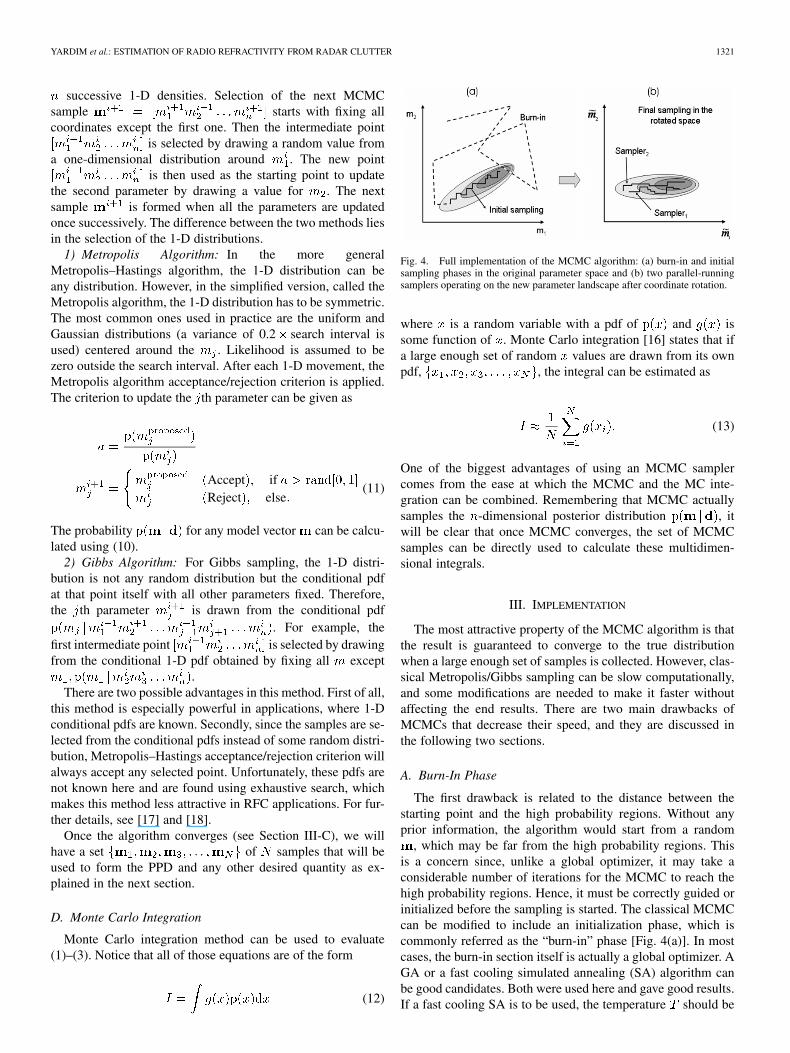
Fig. 4. Full implementation of the MCMC algorithm: (a) burn-in and initialsampling phases in the original parameter space and (b) two parallel-runningsamplers operating on the new parameter landscape after coordinate rotation.

where is a random variable with a pdf of and issome function of . Monte Carlo integration [16] states that ifa large enough set of random values are drawn from its ownpdf, , the integral can be estimated as

(13)

One of the biggest advantages of using an MCMC samplercomes from the ease at which the MCMC and the MC inte-gration can be combined. Remembering that MCMC actuallysamples the -dimensional posterior distribution , itwill be clear that once MCMC converges, the set of MCMCsamples can be directly used to calculate these multidimen-sional integrals.

III. IMPLEMENTATION

The most attractive property of the MCMC algorithm is thatthe result is guaranteed to converge to the true distributionwhen a large enough set of samples is collected. However, clas-sical Metropolis/Gibbs sampling can be slow computationally,and some modifications are needed to make it faster withoutaffecting the end results. There are two main drawbacks ofMCMCs that decrease their speed, and they are discussed inthe following two sections.

A. Burn-In Phase

The first drawback is related to the distance between thestarting point and the high probability regions. Without anyprior information, the algorithm would start from a random

, which may be far from the high probability regions. Thisis a concern since, unlike a global optimizer, it may take aconsiderable number of iterations for the MCMC to reach thehigh probability regions. Hence, it must be correctly guided orinitialized before the sampling is started. The classical MCMCcan be modified to include an initialization phase, which iscommonly referred as the “burn-in” phase [Fig. 4(a)]. In mostcases, the burn-in section itself is actually a global optimizer. AGA or a fast cooling simulated annealing (SA) algorithm canbe good candidates. Both were used here and gave good results.If a fast cooling SA is to be used, the temperature should be

1322 IEEE TRANSACTIONS ON ANTENNAS AND PROPAGATION, VOL. 54, NO. 4, APRIL 2006

lowered until it reaches so that the Boltzmann distribu-tion used for SA actually becomes the likelihood function itselfat that temperature [16]

(14)

B. Initial Sampling and Coordinate Rotation

The second drawback is based on the effects of interparametercorrelation. Recalling that there is freedom of movement onlyin the directions parallel to parameter axes, it is hard to samplehighly correlated PPDs [Fig. 4(a)]. With only vertical and hor-izontal movements allowed, it will take many samples to movefrom one end to the other of the slanted high probability areas,whereas it can be done with a much smaller number of samplesin an uncorrelated case.

The remedy lies in a rotation of coordinate in the -dimen-sional parameter space [19]. Instead of applying Metropolissampling in the correlated parameter space, a new set ofuncorrelated parameters are defined by applying an orthog-onal coordinate transformation that diagonalizes the modelcovariance matrix . The rotation matrix is found byeigenvalue-eigenvector decomposition of

(15)

where is a diagonal matrix containing the eigenvalues of thecovariance matrix, is the orthonormal rotation matrix, whosecolumns contain the eigenvectors of , and is the rotatedmodel vector. The model covariance matrix is found using sam-ples drawn from the PPD after the burn-in phase. Only a smallnumber of MCMC samples (about 1000) are enough to find Cdue to its fast converging nature [5], [14]. This is referred to asthe initial sampling phase. After this phase, the parameter spaceis rotated before the final sampling phase starts.

C. Final Sampling Phase and Convergence

The final sampling phase simply is composed of two inde-pendent, parallel-running Metropolis (or Gibbs) samplers in therotated space, sampling the same PPD [Fig. 4(b)]. The algorithmuses a convergence criterion based on the Kolmogorov–Smirnov(K–S) statistic function of the marginal posterior distributions[20]. s are calculated using (3) as each new sample isdrawn. A pair of , one from each sampler, is calculatedfor each parameter . Then the K–S statistic is calculated foreach parameter as

(16)

where and represent the cumulative mar-ginal distribution functions for the two parallel-running sam-plers. The simulation is assumed to have converged when thelargest term is less than ( is used here). Afterthe convergence criterion is met, these two independent sets arecombined to form a final set twice as large so that the difference

between the true distribution and the estimated one is expectedto be even less.

To use the likelihood (9), the error variance must be esti-mated. In this paper, an estimate for is calculated using an MLapproach. To find the ML estimate of the variance,is solved and evaluated at the ML model estimate . This re-sults in

(17)

itself is estimated using a global optimizer, usually the valueobtained at the end of the burn-in phase.

Equation (17) assumes the measurements at different rangesare uncorrelated, which may not be the case. Gerstoft and Meck-lenbräuker [7] suggested replacing with , number of ef-fectively uncorrelated data points. More detailed discussion canbe found in [14] and [15].

Received clutter power can be calculated as given in [3], interms of the one-way loss term in decibels as

(18)

where is a constant that includes wavelength, radar cross-sec-tion (RCS), transmitter power, antenna gain, etc. If these valuesare known, they can be included into the equation. However,one or more may be unavailable such as the mean RCS or trans-mitter specifications. An alternative, which is used here, is dis-carding these constant terms, which is done by subtracting boththe mean of the replica clutter from itself and the meanof the measured clutter from itself before inserting them intothe likelihood function.

D. Postprocessing

After the MCMC sampler converges with a set of refractivityparameters , a postprocessing sectionis needed to convert the uncertainty in the M-profile into otherparameters of interest that could be used by the radar operator,such as the propagation factor and the one-way propagation loss.

Assume an end-user parameter , which can be expressedas a function of model parameters . The posteriorprobability distribution of PPD can be simply calculated bydrawing a large amount of samples of from its own PPD andcalculating for each one. Then this set of can be usedto obtain the or perform any other uncertainty analysisof using (1)–(3) and MC integration.

Since the usage of an MCMC sampler guarantees thatis a large enough set drawn from its

own PPD, this set can readily be used to obtain the statistics of.

IV. EXAMPLES

This section is composed of both synthetic and experimentalexamples. Four different algorithms, two of which are MCMC,are first tested using synthetic data generated by the terrain par-abolic equation program (TPEM) [8]. Then the data gatheredduring the Wallops’98 Space Range Radar (SPANDAR) mea-surement are analyzed using the Metropolis sampler and GA.

YARDIM et al.: ESTIMATION OF RADIO REFRACTIVITY FROM RADAR CLUTTER 1323

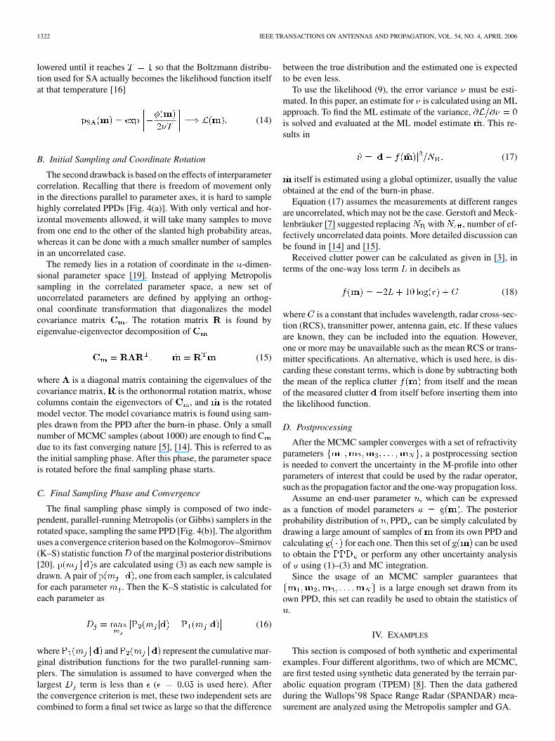
TABLE IISYNTHETIC DATA CASE: GA ESTIMATES AND METROPOLIS ALGORITHM RESULTS

Fig. 5. Initial sampling phase—convergence of the model covariance matrixin terms of percent error.C later will be used for coordinate rotation.

A. Algorithm Validation

To validate the MCMC algorithms, a comparison with the truedistribution is necessary. The true distribution can be obtainedby using exhaustive search; however, it is extremely inefficientand demands a large number of forward model runs. Even ifonly 25 discrete possible values are assumed for each of thefour parameters used for the model in Fig. 2, the state spaceconsists of (390 k) possible states. A simplerange-independent trilinear model with only four parameters isused since an exhaustive search would need around 10 000-kforward model runs for five parameters. The number of forwardmodel runs needed for MCMC is proportional to the dimensionsize, so as dimension size increases, it requires much fewer sam-ples than the exhaustive search. The selected parameters are theslope and height of the base layer ( and ) and the slopeand thickness of the inversion layer ( and ), as shown inFig. 3. Their test case values and the search bounds are given inTable II. A standard atmosphere with a vertical refractivity gra-dient (top layer slope) of 0.118 M-units/m is assumed above theinversion layer. Parameters are selected in terms of the heightsand slopes instead of the classical heights and widths (such asthe frequently used inversion thickness and M-deficit) due totheir relatively smaller interparameter correlation.

The synthetic data are generated by TPEM at a frequency of2.84 GHz, antenna 3-dB beamwidth of 0.4 , source height of30.78 m, and radar clutter standard deviation of 10 dB, a typicalvalue reported also in [21]. Inversion is done using four differentmethods for a range of 10–60 km.

Fig. 6. Final sampling phase: Kolmogorov–Smirnov statistic D for eachparameter. Used for the convergence of the posterior probability density.

The convergence characteristics of both MCMC algorithmsare similar. The results of the initial sampling phase are given inFig. 5 in terms of a convergence plot for the model covariancematrix . The percent error is calculated as the average abso-lute percent change in all matrix entries of as the matrix isrecalculated while new samples are taken. The matrix convergesquickly and for this case, only 250 samples were sufficient tohave a good estimate of .

After the rotation matrix is obtained, two independentMetropolis/Gibbs algorithms run during the final samplingphase until the convergence criterion given in Section III-Care met (Fig. 6). Dosso [5] reported convergence in 7 10(700 k) forward models with a Gibbs sampler and around 100 kwith a fast Gibbs sampler (FGS). Similarly, Battle et al. [15]reported convergence in 63-k models using a less strict conver-gence criterion, again with an FGS. Due to the modificationsin the Metropolis/Gibbs algorithms used here, they also canbe classified as “fast” samplers. Therefore, a typical value of100-k models is in agreement with the previous applications ofMCMC algorithms. During the simulations, values as low as20-k models and higher than 150-k models were encountered.

The marginal distributions of the four parameters are givenFig. 7. Except for exhaustive search, the results for all othersare calculated using the MC integration. The exhaustive searchresult [Fig. 7(a)] is obtained with 25 discrete values per param-eter and 390-k samples, whereas both Metropolis [Fig. 7(b)] andGibbs [Fig. 7(c)] samplers use approximately 70-k samples andthe genetic algorithm [Fig. 7(d)] uses less than 10-k samples.

1324 IEEE TRANSACTIONS ON ANTENNAS AND PROPAGATION, VOL. 54, NO. 4, APRIL 2006

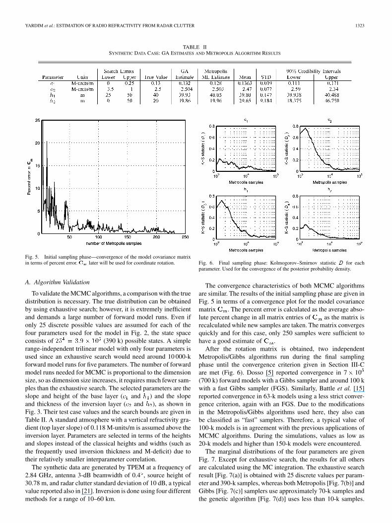
Fig. 7. Marginal posterior probability distributions for the synthetic test case.Vertical lines show the true values of the parameters. (a) Exhaustive search, (b)Metropolis algorithm, (c) Gibbs algorithm, and (d) genetic algorithm.

The results of the Metropolis algorithm and GA are also sum-marized in Table II. The MATLAB GA toolbox [22] is used forGA results. It uses three isolated populations of size 40 eachwith a migration rate of 0.025 per ten generations, a mutationrate of 0.10 and a crossover fraction of 0.8.

All four algorithms have almost identical ML estimates forthe parameters. However, it should be noted that MCMC sam-plers converged after collecting nearly seven times more sam-ples than GA. On the other hand, the distributions obtained fromthe MCMC samplers are closer to the true distributions given byexhaustive search.

Marginal and two-dimensional (2-D) posterior distributionsobtained by the Metropolis sampler are given in Fig. 8. The di-agonal pdfs are the 1-D marginal pdfs and the off-diagonal plotsare the 2-D marginal pdfs, where the 50, 75, and 95% highestposterior density (HPD) regions are plotted, with the ML so-lution points (white crosses). In Bayesian statistics, credibilityintervals and HPD regions are used to analyze the posterior dis-tributions. They are very similar to the confidence interval andtheir definitions can be found in [23].

B. Wallops Island Experiment

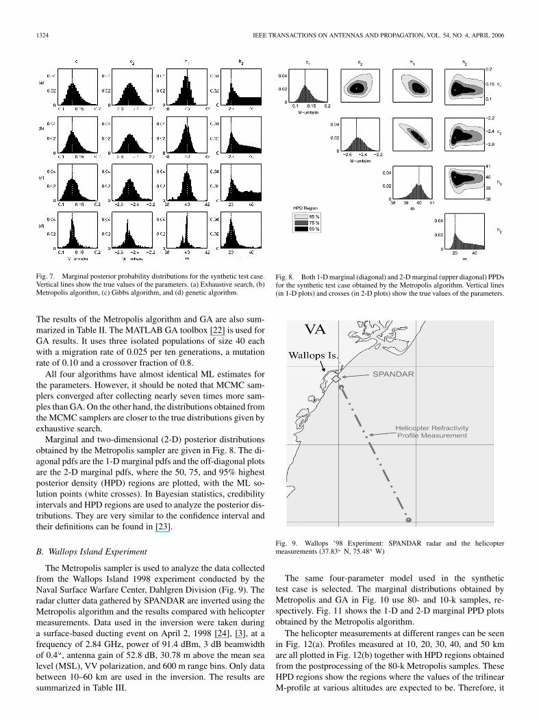
The Metropolis sampler is used to analyze the data collectedfrom the Wallops Island 1998 experiment conducted by theNaval Surface Warfare Center, Dahlgren Division (Fig. 9). Theradar clutter data gathered by SPANDAR are inverted using theMetropolis algorithm and the results compared with helicoptermeasurements. Data used in the inversion were taken duringa surface-based ducting event on April 2, 1998 [24], [3], at afrequency of 2.84 GHz, power of 91.4 dBm, 3 dB beamwidthof 0.4 , antenna gain of 52.8 dB, 30.78 m above the mean sealevel (MSL), VV polarization, and 600 m range bins. Only databetween 10–60 km are used in the inversion. The results aresummarized in Table III.

Fig. 8. Both 1-D marginal (diagonal) and 2-D marginal (upper diagonal) PPDsfor the synthetic test case obtained by the Metropolis algorithm. Vertical lines(in 1-D plots) and crosses (in 2-D plots) show the true values of the parameters.

Fig. 9. Wallops ’98 Experiment: SPANDAR radar and the helicoptermeasurements (37.83 N, 75.48 W)

The same four-parameter model used in the synthetictest case is selected. The marginal distributions obtained byMetropolis and GA in Fig. 10 use 80- and 10-k samples, re-spectively. Fig. 11 shows the 1-D and 2-D marginal PPD plotsobtained by the Metropolis algorithm.

The helicopter measurements at different ranges can be seenin Fig. 12(a). Profiles measured at 10, 20, 30, 40, and 50 kmare all plotted in Fig. 12(b) together with HPD regions obtainedfrom the postprocessing of the 80-k Metropolis samples. TheseHPD regions show the regions where the values of the trilinearM-profile at various altitudes are expected to be. Therefore, it

YARDIM et al.: ESTIMATION OF RADIO REFRACTIVITY FROM RADAR CLUTTER 1325

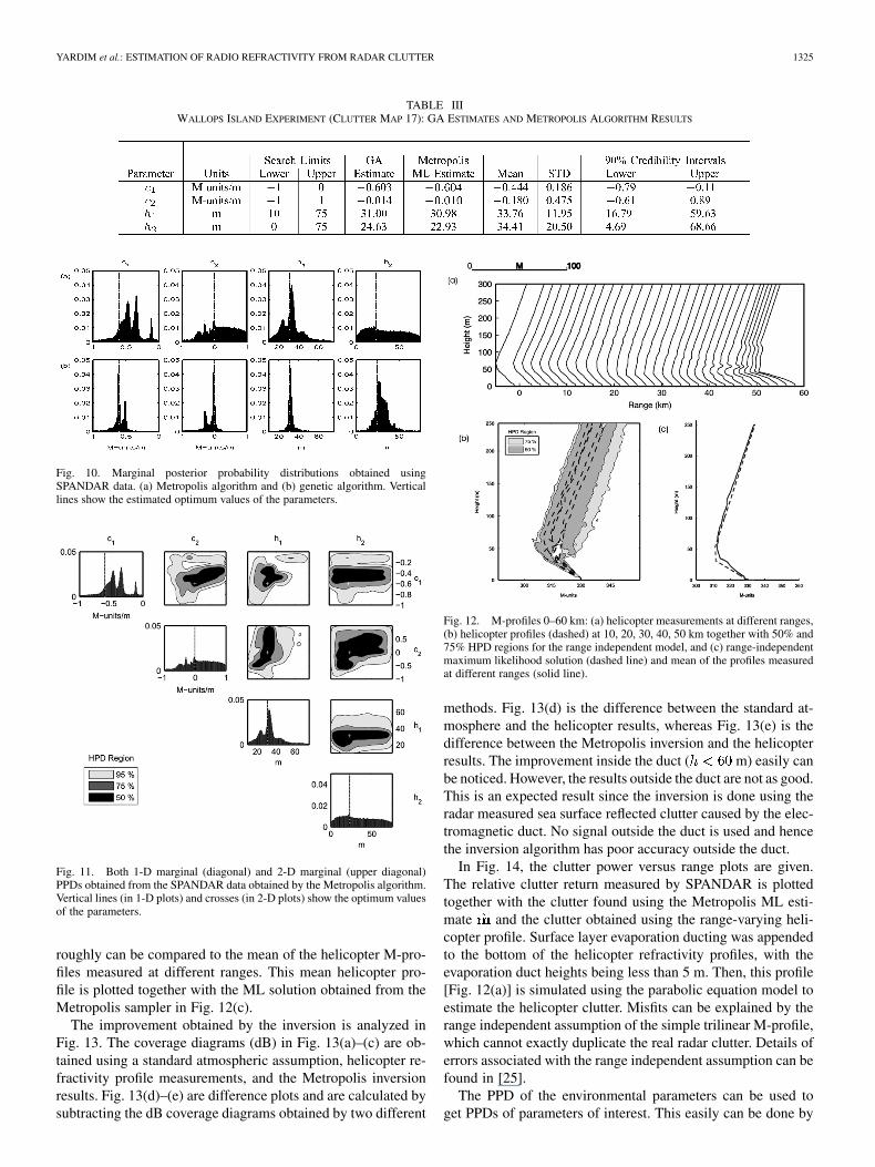
TABLE IIIWALLOPS ISLAND EXPERIMENT (CLUTTER MAP 17): GA ESTIMATES AND METROPOLIS ALGORITHM RESULTS

Fig. 10. Marginal posterior probability distributions obtained usingSPANDAR data. (a) Metropolis algorithm and (b) genetic algorithm. Verticallines show the estimated optimum values of the parameters.

Fig. 11. Both 1-D marginal (diagonal) and 2-D marginal (upper diagonal)PPDs obtained from the SPANDAR data obtained by the Metropolis algorithm.Vertical lines (in 1-D plots) and crosses (in 2-D plots) show the optimum valuesof the parameters.

roughly can be compared to the mean of the helicopter M-pro-files measured at different ranges. This mean helicopter pro-file is plotted together with the ML solution obtained from theMetropolis sampler in Fig. 12(c).

The improvement obtained by the inversion is analyzed inFig. 13. The coverage diagrams (dB) in Fig. 13(a)–(c) are ob-tained using a standard atmospheric assumption, helicopter re-fractivity profile measurements, and the Metropolis inversionresults. Fig. 13(d)–(e) are difference plots and are calculated bysubtracting the dB coverage diagrams obtained by two different

Fig. 12. M-profiles 0–60 km: (a) helicopter measurements at different ranges,(b) helicopter profiles (dashed) at 10, 20, 30, 40, 50 km together with 50% and75% HPD regions for the range independent model, and (c) range-independentmaximum likelihood solution (dashed line) and mean of the profiles measuredat different ranges (solid line).

methods. Fig. 13(d) is the difference between the standard at-mosphere and the helicopter results, whereas Fig. 13(e) is thedifference between the Metropolis inversion and the helicopterresults. The improvement inside the duct ( m) easily canbe noticed. However, the results outside the duct are not as good.This is an expected result since the inversion is done using theradar measured sea surface reflected clutter caused by the elec-tromagnetic duct. No signal outside the duct is used and hencethe inversion algorithm has poor accuracy outside the duct.

In Fig. 14, the clutter power versus range plots are given.The relative clutter return measured by SPANDAR is plottedtogether with the clutter found using the Metropolis ML esti-mate and the clutter obtained using the range-varying heli-copter profile. Surface layer evaporation ducting was appendedto the bottom of the helicopter refractivity profiles, with theevaporation duct heights being less than 5 m. Then, this profile[Fig. 12(a)] is simulated using the parabolic equation model toestimate the helicopter clutter. Misfits can be explained by therange independent assumption of the simple trilinear M-profile,which cannot exactly duplicate the real radar clutter. Details oferrors associated with the range independent assumption can befound in [25].

The PPD of the environmental parameters can be used toget PPDs of parameters of interest. This easily can be done by

1326 IEEE TRANSACTIONS ON ANTENNAS AND PROPAGATION, VOL. 54, NO. 4, APRIL 2006

Fig. 13. Coverage diagrams (dB). One-way propagation loss for (a) standardatmosphere (0.118 M-units/m), (b) helicopter-measured refractivity profile, and(c) Metropolis inversion result. The difference (dB) between (d) helicopter andstandard atmosphere results and (e) helicopter and Metropolis inversion results.

Fig. 14. Clutter power versus range plots. Clutter measured by SPANDAR(solid), the predicted clutter obtained using the Metropolis ML solution m̂(dashed), and the predicted clutter obtained using the helicopter-measuredrefractivity profile (dotted).

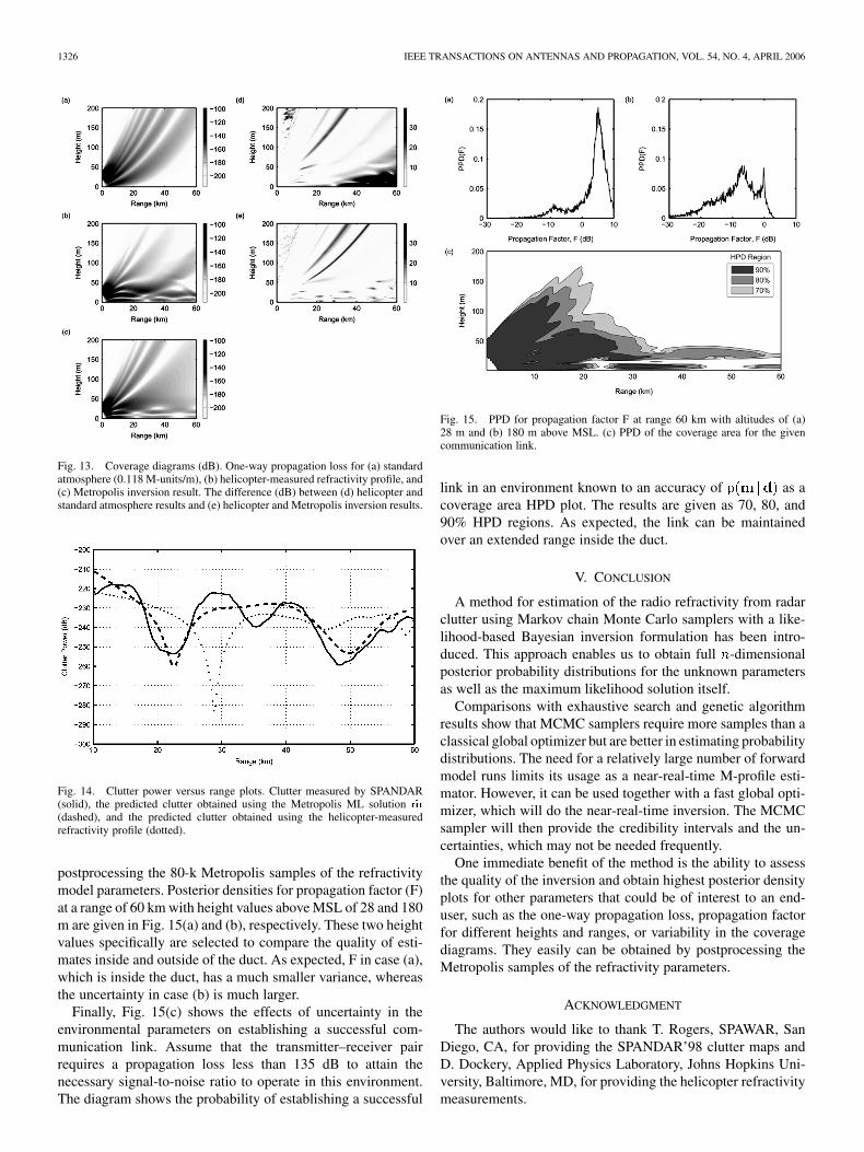
postprocessing the 80-k Metropolis samples of the refractivitymodel parameters. Posterior densities for propagation factor (F)at a range of 60 km with height values above MSL of 28 and 180m are given in Fig. 15(a) and (b), respectively. These two heightvalues specifically are selected to compare the quality of esti-mates inside and outside of the duct. As expected, F in case (a),which is inside the duct, has a much smaller variance, whereasthe uncertainty in case (b) is much larger.

Finally, Fig. 15(c) shows the effects of uncertainty in theenvironmental parameters on establishing a successful com-munication link. Assume that the transmitter–receiver pairrequires a propagation loss less than 135 dB to attain thenecessary signal-to-noise ratio to operate in this environment.The diagram shows the probability of establishing a successful

Fig. 15. PPD for propagation factor F at range 60 km with altitudes of (a)28 m and (b) 180 m above MSL. (c) PPD of the coverage area for the givencommunication link.

link in an environment known to an accuracy of as acoverage area HPD plot. The results are given as 70, 80, and90% HPD regions. As expected, the link can be maintainedover an extended range inside the duct.

V. CONCLUSION

A method for estimation of the radio refractivity from radarclutter using Markov chain Monte Carlo samplers with a like-lihood-based Bayesian inversion formulation has been intro-duced. This approach enables us to obtain full -dimensionalposterior probability distributions for the unknown parametersas well as the maximum likelihood solution itself.

Comparisons with exhaustive search and genetic algorithmresults show that MCMC samplers require more samples than aclassical global optimizer but are better in estimating probabilitydistributions. The need for a relatively large number of forwardmodel runs limits its usage as a near-real-time M-profile esti-mator. However, it can be used together with a fast global opti-mizer, which will do the near-real-time inversion. The MCMCsampler will then provide the credibility intervals and the un-certainties, which may not be needed frequently.

One immediate benefit of the method is the ability to assessthe quality of the inversion and obtain highest posterior densityplots for other parameters that could be of interest to an end-user, such as the one-way propagation loss, propagation factorfor different heights and ranges, or variability in the coveragediagrams. They easily can be obtained by postprocessing theMetropolis samples of the refractivity parameters.

ACKNOWLEDGMENT

The authors would like to thank T. Rogers, SPAWAR, SanDiego, CA, for providing the SPANDAR’98 clutter maps andD. Dockery, Applied Physics Laboratory, Johns Hopkins Uni-versity, Baltimore, MD, for providing the helicopter refractivitymeasurements.

YARDIM et al.: ESTIMATION OF RADIO REFRACTIVITY FROM RADAR CLUTTER 1327

REFERENCES

[1] S. Vasudevan and J. Krolik, “Refractivity estimation from radar clutterby sequential importance sampling with a Markov model for microwavepropagation,” in Proc. ICASSP, 2001, pp. 2905–2908.

[2] R. Anderson, S. Vasudevan, J. Krolik, and L. T. Rogers, “Maximuma posteriori refractivity estimation from radar clutter using a Markovmodel for microwave propagation,” in Proc. IEEE Int. Geosci. RemoteSens. Symp., vol. 2, Sydney, Australia, 2001, pp. 906–909.

[3] P. Gerstoft, L. T. Rogers, J. Krolik, and W. S. Hodgkiss, “Inversion forrefractivity parameters from radar sea clutter,” Radio Sci., vol. 38, no.18, pp. 1–22, 2003.

[4] P. Gerstoft, W. S. Hodgkiss, L. T. Rogers, and M. Jablecki, “Probabilitydistribution of low altitude propagation loss from radar sea-clutter data,”Radio Sci., vol. 39, pp. 1–9, 2004.

[5] S. E. Dosso, “Quantifying uncertainty in geoacoustic inversion I: A fastGibbs sampler approach,” J. Acoust. Soc. Amer., vol. 111, no. 1, pp.129–142, 2002.

[6] L. T. Rogers, M. Jablecki, and P. Gerstoft, “Posterior distributions of astatistic of propagation loss inferred from radar sea clutter,” Radio Sci.,2005.

[7] P. Gerstoft and C. F. Mecklenbräuker, “Ocean acoustic inversion with es-timation of a posteriori probability distributions,” J. Acoust. Soc. Amer.,vol. 104, no. 2, pp. 808–819, 1998.

[8] A. E. Barrios, “A terrain parabolic equation model for propagation in thetroposphere,” IEEE Trans. Antennas Propag., vol. 42, no. 1, pp. 90–98,1994.

[9] M. Levy, Parabolic Equation Methods for Electromagnetic Wave Prop-agation, London, U.K.: Institution of Electrical Engineers, 2000.

[10] S. M. Kay, Fundamentals of Statistical Signal Processing—Volume I:Estimation Theory. Englewood Cliffs, NJ: Prentice-Hall, 1993.

[11] M. K. Sen and P. L. Stoffa, “Bayesian inference, Gibbs’ sampler anduncertainty estimation in geophysical inversion,” Geophys. Prosp., vol.44, pp. 313–350, 1996.

[12] N. Metropolis, A. W. Rosenbluth, M. N. Rosenbluth, A. H. Teller, andE. Teller, “Equation of state calculations by fast computing machines,”J. Chem. Phys., vol. 21, pp. 1087–1092, 1953.

[13] S. Geman and D. Geman, “Stochastic relaxation, Gibbs distributions,and the Bayesian restoration of images,” IEEE Trans. Pattern Anal. Ma-chine Intell., vol. 6, pp. 721–741, 1984.

[14] S. E. Dosso and P. L. Nielsen, “Quantifying uncertainty in geoacousticinversion II. Application to broadband, shallow-water data,” J. Acoust.Soc. Amer., vol. 111, no. 1, pp. 143–159, 2002.

[15] D. J. Battle, P. Gerstoft, W. S. Hodgkiss, W. A. Kuperman, and P. L.Nielsen, “Bayesian model selection applied to self-noise geoacousticinversion,” J. Acoust. Soc. Amer., vol. 116, no. 4, pp. 2043–2056, Oct.2004.

[16] J. J. K. O. Ruanaidh and W. J. Fitzgerald, Numerical BayesianMethods Applied to Signal Processing, ser. Statistics and ComputingSeries. New York: Springer-Verlag, 1996.

[17] K. Mosegaard and M. Sambridge, “Monte Carlo analysis of inverseproblems,” Inv. Prob., vol. 18, no. 3, pp. 29–54, 2002.

[18] D. J. C. MacKay, Information Theory, Inference and Learning Algo-rithms. Cambridge, U.K.: Cambridge Univ. Press, 2003.

[19] M. D. Collins and L. Fishman, “Efficient navigation of parameter land-scapes,” J. Acoust. Soc. Amer., vol. 98, pp. 1637–1644, 1995.

[20] W. H. Press, S. A. Teukolsky, W. T. Vetterling, and B. Flannery, Numer-ical Recipes in C, 2nd ed. Cambridge, U.K.: Cambridge Univ. Press,1995.

[21] K. D. Anderson, “Radar detection of low-altitude targets in a maritimeenvironment,” IEEE Trans. Antennas Propag., vol. 43, pp. 609–613, Jun.1995.

[22] D. E. Goldberg, Genetic Algorithms in Search, Optimization and Ma-chine Learning. Reading, MA: Addison-Wesley, 1989.

[23] G. E. P. Box and G. C. Tiao, Bayesian Inference in Statistical Anal-ysis. New York: Addison-Wesley, 1992.

[24] L. T. Rogers, C. P. Hattan, and J. K. Stapleton, “Estimating evaporationduct heights from radar sea echo,” Radio Sci., vol. 35, no. 4, pp. 955–966,2000.

[25] J. Goldhirsh and D. Dockery, “Propagation factor errors due to the as-sumption of lateral homogenity,” Radio Sci., vol. 33, no. 2, pp. 239–249,1998.

Caglar Yardim (S’98) was born in Ankara, Turkey,on December 5, 1977. He received the B.S. and M.S.degrees in electrical engineering from the MiddleEast Technical University (METU), Ankara, in 1998and 2001, respectively. He is currently pursuingthe Ph.D. degree at the Electrical and ComputerEngineering Department, University of California,San Diego.

From 1998 to 2000, he was a Research Assistantwith METU. From 2000 to 2002, he was a ResearchEngineer with the Microwave and System Technolo-

gies Division, ASELSAN Electronic Industries Inc. Since 2002, he has been aGraduate Research Associate with the Marine Physical Laboratory, Universityof California, San Diego. His research interests include propagation, optimiza-tion, modeling, and inversion of electromagnetic signals.

Peter Gerstoft received the M.Sc. and Ph.D. degreesfrom the Technical University of Denmark, Lyngby,in 1983 and 1986, respectively, and the M.Sc. degreefrom the University of Western Ontario, London, ON,Canada, in 1984.

From 1987 to 1992, he was with Ødegaardand Danneskiold-Samsøe, Copenhagen, Denmark,working on forward modeling and inversion forseismic exploration, with a year as a Visiting Sci-entist at the Massachusetts Institute of Technology,Cambridge. From 1992 to 1997, he was Senior

Scientist at SACLANT Undersea Research Centre, La Spezia, Italy, where hedeveloped the SAGA inversion code, which is used for ocean acoustic andelectromagnetic signals. Since 1997, he has been with the Marine PhysicalLaboratory, University of California, San Diego. His research interests includeglobal optimization, modeling, and inversion of acoustic, elastic, and electro-magnetic signals.

Dr. Gerstoft is a Fellow of the Acoustical Society of America and an electedmember of the International Union of Radio Science, Commission F.

William S. Hodgkiss (S’68–M’75) was born inBellefonte, PA, on August 20, 1950. He received theB.S.E.E. degree from Bucknell University, Lewis-burg, PA, in 1972 and the M.S. and Ph.D. degreesin electrical engineering from Duke University,Durham, NC, in 1973 and 1975, respectively.

From 1975 to 1977, he was with the Naval OceanSystems Center, San Diego, CA. From 1977 to1978, he was a Faculty Member in the ElectricalEngineering Department, Bucknell University. Since1978, he has been a Member of the Faculty, Scripps

Institution of Oceanography, University of California, San Diego, and on thestaff of the Marine Physical Laboratory, where he is currently Deputy Director.His present research interests are in the areas of adaptive array processing,propagation modeling, and environmental inversions with applications of thoseto underwater acoustics and electromagnetic wave propagation.

Dr. Hodgkiss is a Fellow of the Acoustical Society of America.