In Imaging Spectrometry X, Proceedings of SPIE Vol. 5159

August 2003.

1

Clutter modeling for subsurface detection in hyperspectral imagery using Markov random fields

Yahya M. Masalmah, Miguel Vélez-Reyes1, and Luis O. Jiménez-Rodríguez

Laboratory for Applied Remote Sensing and Image Processing, University of Puerto Rico at Mayagüez, P.O. Box 9042, Mayagüez, Puerto Rico 00681-9042

1 m.velez@ieee.org; phone +1.787.832.1105; fax +1.787.832.1275

ABSTRACT

Hyperspectral imagery provides high spectral and spatial resolution that can be used to discriminate between object and clutter occurring in subsurface remote sensing for applications such as environmental monitoring and biomedical imaging. We look at using a noncausal auto-regressive Gauss-Markov Random Field (GMRF) model to model clutter produced by a scattering media for subsurface estimation, classification, and detection problems. The GMRF model has the advantage that the clutter covariance only depends on 4 parameters regardless of the number of bands used. We review the model and parameter estimation methods using least squares and approximate maximum likelihood. Experimental and simulation model identification results are presented. Experimental data is generated by using a subsurface testbed where an object is placed in the bottom of a fish tank filled with water mixed with TiO2 to simulate a a mild to high scattering environment. We show that, for the experimental data, least square estimates produce good models for the clutter. When used in a subsurface classification problem, the GMRF model results in better broad classification with loss of some spatial structure details when compared to spectral only classification.

Keywords: Hyperspectral Imagery, Subsurface Detection, Markov Random Fields

1. INTRODUCTION Hyperspectral sensors collect hundreds of narrow and contiguously spaced spectral bands of data organized in the so called hyperspectral cube. Hyperspectral imagery provides fully registered spatial and high resolution spectral information that is invaluable in discriminating between objects and natural clutter backgrounds, since the objects and the clutter have unique spectral signatures that are captured by the data as illustrated in Figure 1 [1]. Our focus is on using hyperspectral sensor data for the detection of parameters of objects in subsurface applications. One of the key problems with HSI is the high dimensionality of the data which results in the need of a large number of training samples for classifiers. In this paper, we present the use of a Gaussian Random Field Model, motivated by [2,3,4], for detecting objects embedded in a scattering media. The advantage of this model is that the resulting covariance matrix is parameterized by 4 parameters, significantly reducing the number of training samples required for classifier training. This type of detection problem arises in coastal environments and biomedical applications.

Figure 1: Hyperspectral imagery concept [1].

1.1 Literature Review In the literature, algorithms for HSI classification can be grouped in two major categories: spectral-only and spatial-spectral algorithms.

1.1.1 Spectral-only algorithms In this type of algorithms, only spectral information from each individual pixel is being used by detection and classification algorithms. The algorithms can be based on linear mixture models [5] or statistical approaches such as the spectral matched filter (SMF) [5,6], or the spectral angle mapper (SAM) [5]. SMF and SAM algorithms depend on knowing a priori, the spectral signature of the target of interest. SMF processes the data by correlating the known signature with the measured signature at every pixel in the data set, while SAM measures the angle between the known signature and the measured signature at each pixel. Those locations where the measured signature is highly correlated with the known signature, or has the smallest angle, are considered targets. Both algorithms ignore the spatial information, and do not account for target signature variability due to factors such as atmospheric and illumination effects.

M

K

N

(i,j,k) (i, j+1, k) (i, j-1, k)

(i-1, j, k)

(i+1, j, k)

(i,j,k+1)

(i,j,k-1)

Figure 2: Three -dimensional rectangular lattice. Figure 3: Neighboring system.

1.1.2 Spatial-Spectral algorithms Another type of HSI information extraction algorithms are those that use both spatial and spectral features. In [7], an adaptive spatial/spectral detection algorithm is presented where the clutter model includes spatial and spectral correlation. The method uses a separate spatial matched filter for each spectral band to adapt to the clutter before using Maximum-likelihood (ML) ratio to perform the detection. The algorithm requires taking the inverse of a spectral covariance matrix which has a dimension equal to the number of spectral bands used for processing. Another approach which employs Gauss-Markov random fields [3,4] was introduced as an extension of noncausal Gauss-Markov Fields [8] to hyperspectral imagery. An adaptive anomaly detection algorithm that is computationally efficient and exhibits a low false alarm rate with high detection probability was designed. In [3,4], a 3-D GMRF was employed to construct a covariance matrix with simple parameterization and is used here as the basis for the presented subsurface detection work.

2. MARKOV RANDOM FIELD MODELING OF HSI Each pixel in the hyperspectral image can be represented by three indices: two spatial and one spectral. In a stochastic representation, the hyperspectral image is considered to be a sample of a 3D array of random variables called a random field (RF) [9] (see Figure 2). Let L be the set of indices in a 3-D lattice, then the random variables can be described by

, sX x s L= ∈ (1)

where L is the set of lattice indexes given by

( , , ):1 ,1 ,1L i j k i N j M k K= ≤ ≤ ≤ ≤ ≤ ≤ (2)

A Markov random field (MRF) is a random field for which the conditional probabilities of the random variables in the field depend only on the variables in the neighboring system [10]

( | ,( , , ) ) ( | ,( , , ) )ijk ijkijk lmn ijk lmnp x x l m n L p x x l m n η∈ = ∈ (3)

where ηijk is the neighborhood of the ijk-th pixel. A Gauss-Markov random field (GMRF) is a Markov random field where all conditional probabilities density distributions are Gaussian. A GMRF model have been proposed in [2,3,4] using the nearest spectral and spatial neighbors as shown in Figure 3 and is given by

ijkkijkijsjkijkivkjikjihijk xxxxxxx εβββ ++++++= +−+−+− )()()( )!()1()1()1()1()1( (4)

where parameters ßh, ßv, and ßs are the MMSE predictor coefficient for the spatial and spectral neighbors respectively (see Figure 3), and ?ijk is a gaussian prediction error sequence. During processing, the image is spatially divided in smaller HSI cubes of dimension Ni×Nj×Nk where it is assumed that the clutter is homogeneous. For each minicube, the parameters of (4) are estimated using one of various methods as we shall see later. On the boundaries between windows, a Dirichlet boundary condition is assumed [11]. Based on these assumptions, equation (4) can be represented in a matrix format for each individual window as follows

Ax=ε (5) where x is a Ni Nj Nk ×1 vector constructed by arranging the mini HSI cube data in a vector format,

1 2

2 1

2

2 1

. 0. . .

0 . .

A AA A

AA

A A

=

21

1 AHAIkk NN ⊗+⊗= (6)

⊗ is the Kronecker product [12], and

CHBIAii NN ⊗+⊗= 1

1 (7)

DIAiN ⊗=2 (8)

The matrices B, C, and D are defined as follows

jj NNh IHB +−= 1β (9)

jNv IC β−= (10)

jNs ID β−= (11)

where Im, is an m×m identity matrix, and Hm is an m×m Toeplitz matrix which has zeros everywhere except for ones on the upper and lower diagonals. The matrix A is called the potential matrix in the literature. The matrix A is a sparse block-tridiagonal matrix that contains all the relevant information regarding GMRF structure [11]. We will further assume that the error vector ? is zero mean with covariance matrix given by

Σε =σ2A.

this leads to a direct parameterization of the inverse of the clutter covariance matrix, 1−Σ x , as follows

AAAx 211 1

σε =Σ=Σ −− (12)

Using (6)-(11) and Kronecker product identities, equation (12) can be rewritten as

( ) ( ) ( ) ( )jtkjtkjtkjtk NNN

zNNN

vNNNNNN

hx IIHIHIIIIHII ⊗⊗−⊗⊗−⊗⊗+⊗⊗−=Σ− 1

21

221

21 1

σβ

σβ

σσβ

(13)

The above equations show that the parameterization of the inverse of the clutter covariance matrix is also only a function of βh, βv, βs, and σ2. The proposed GMRF model represents a trade-off between model complexity and prediction uncertainty as is commonly discussed in system identification [13]. Our hope is that the simple model described by (4) with the corresponding simple noise assumption will allow us to achieve improved classification or detection in HSI.

3. PARAMETER ESTIMATION The parameters of the model (4) can be estimated using one of the following techniques: Maximum Likelihood(ML) , Approximate Maximum Likelihood (AML) , and Least squares (LS). Each methodology, as we shall see, represents a tradeoff between computational complexity and optimality of the resulting estimate. Once the parameters are estimated, binary hypothesis testing, or other testing algorithms could be used to detect the targets.

3.1 Maximum Likelihood Estimation Under Gaussian assumptions for ε, the likelihood function is given by

( ) ( ) 2/122 2lnln

21

L 21 nT πσ

σ−−−= −AAxx? (14)

where

[ ]Tsvh2σβββ=?

and n=Ni×Nj×Nk. Maximum likelihood (ML) estimation is based on maximization of the function L(θ) subject to the constraint that A is positive definite.

( )?? LML maxargˆ =

Computing the ML estimate requires nonlinear optimization.

3.2 Approximate Maximum Likelihood Estimation (AML) Since the determinant of a matrix is the product of its eigenvalues, we can use this fact to find an approximation to (14), which leads to a direct method to compute an approximation to the ML estimate. Using properties of the Kronecker product [12], an analytical expression for the eigenvalues of the matrix A was found in [4] and is given by

( )

+

−

+

−

+−=

1cos2

1cos2

1cos21

ks

iv

jhq N

kN

iN

jA

πβ

πβ

πβλ for q=1,2,3, …, n (15)

where 1≤j≤Nj, 1≤i≤Ni, and 1≤k≤Nk. Notice that, since A is symmetric, the positive definite constraint on A is equivalent to require that all of its eigenvalues are positive, which using (15) can be re-stated as

21

1cos

1cos

1cos ≥

+

+

+

+

+ ks

iv

jh N

kN

iN

j πβ

πβ

πβ (16)

for all ≤j≤Nj, 1≤i≤Ni, and 1≤k≤Nk. In terms of the eigenvalues, the determinant of σ2A is given by

∑∑∑= = =

+

−

+

−

+−+=

i j kN

i

N

j

N

k ks

iv

jh N

kN

iN

jnA

1 1 1

22/12

1cos2

1cos2

1cos21lnln

2ln

πβ

πβ

πβσσ (17)

By using the first few terms of the natural logarithm Taylor series expansion of ln(1-ϕ) around zero, an approximation to equation (17) is suggested in [4] as follows

2)1ln(

2φφφ −−≈− (18)

where

+

+

+

+

+=

1cos2

1cos2

1cos2

ks

iv

jh N

kN

iN

j πβ

πβ

πβφ

Further simplification is achieved by using the following trigonometric identities,

∑=

=

+

N

i Ni

1

01

cosπ

and ∑=

−=

+

N

i

NNi

1

2

21

1cos

π

which results in an approximation to the likelihood function (14) as follows

( ) ( ) 2/22222AML 2ln

111ln

221

L n

k

ks

i

iv

j

jhkji

T

NN

NN

N

NNNN

nπβββσ

σ−

−+

−+

−−−−= Axx? (19)

Notice that this function is quadratic in the parameters βh, βv, and βs so that a direct method to compute these parameters estimate is possible. Approximate Maximum likelihood (ML) estimation is based on maximization of the function LAML(θ) subject to the constraint that A is positive definite.

( )?? AMLAML Lmaxargˆ =

The expressions for the estimates are derived by solving the system of equations that result from taking the derivatives of (19) with respect to the parameters and equating them to zero. The resulting estimates are given by

)1(ˆˆ

2, −=

jkiaml

hamlh NNNσ

χβ (20)

)1(ˆˆ

2, −=

ikjaml

vamlv NNNσ

χβ (21)

)1(ˆˆ

2, −=

kjiaml

samls NNNσ

χβ (22)

pApnxx ml

n

pml

−=−

∑= ˆ'1ˆ1

2σ (23)

where

∑∑∑= = =

+=i j kN

i

N

j

N

kkjiijkh xx

1 1 1)1(χ (24)

∑∑∑−

= = =+=

1

1 1 1)1(

i j kN

i

N

j

N

kjkiijkv xxχ (25)

∑∑ ∑= =

−

=+=

i j kN

i

N

j

N

kkijijks xx

1 1

1

1)1(χ (26)

are the “one- step- ahead” correlation values computed from the data in the Markov window being analyzed.

Since the Taylor series expansion approximation in equation (18) is valid when |ϕ| is much smaller than one, the above expressions for βh, βv, and βs are also valid for the same condition, which is true when the data are weakly correlated. HSI data are highly correlated especially in the spectral dimension so this assumption needs to be revised. When ϕ is not small, an adjustment for the expressions (20)-(23) was derived in [3] and are given by

)1

cos()1

cos()1

cos(

^

++

++

+

=

js

jv

jh

hh

NNNπ

χαπ

χπ

χ

ξχβ (27)

)1

cos()1

cos()1

cos(

^

++

++

+

=

js

jv

jh

vv

NNNπ

χαπ

χπ

χ

ξχβ (28)

^

cos( ) cos( ) cos( )1 1 1

ss

h v sj j jN N N

αξχβ

π π πχ χ α χ=

+ ++ + +

(29)

δξ

α

−=

−−

=

5.0

)1()1(

kj

jk

NNNN

(30)

where δ is a small number included to ensure that the estimates meet the positive definite constraints for A.

3.2.1 Least Squares(LS) The linear least squares (LS) method is a popular method to compute an estimate of the coefficients of a linear model such as (4). The estimate is the value of βh, βv, and βs which minimize the function

( ) 2

2V Axß = (31)

were β=[βh, βv, βs]T. The least squares estimate is obtained by deriving (31) with respect to α and is given by [14]

( ) xGGGß T1T −=LS

ˆ (32)

where

[ ]xTxTxTG 321= (33) 1

1 k i jN N NT I I H= ⊗ ⊗ (34)

12 k i jN N NT I H I= ⊗ ⊗ (35)

13 k i jN N NT H I I= ⊗ ⊗ (36)

4 k i jN N NT I I I= ⊗ ⊗ (37)

The least square estimate is computationally simple but does not have the statistical optimality properties of the ML estimate. Later in the experimental results section, we will use equation (23) with the least square estimates for β to compute an estimate for σ2.

4. PARAMETER ESTIMATION: EXPERIMENTAL RESULTS To study the performance of the parameter estimation algorithms, simulated and real data were used. Simulated data allows us to evaluate the performance of the parameter estimation algorithms under controlled conditions and check some of the modeling assumptions while real data allows us to study the usefulness of the model under realistic conditions. Because of their computational simplicity, only the AML and LS parameter estimation procedures are studied.

4.1 Experiments with Simulated Data In this section, we present results using synthetic data generated using model (4) for different levels of spectral and spatial correlation. The synthetic cube consists of 26 bands and of spatial dimensions of 300×300 pixels. The parameters are βh=0.02, βv=0.01, βs=0.1, and σ2=1. One “band” of the synthetic image is shown in Figure 4.

Figure 4: Synthetic image of 26 bands with parameters βh=0.02, βv=0.01, βs=0.1, and σ2=1.

Table 1: True and estimated values of the model parameters using the synthetic image.

hβ νβ sβ 2σ

True 0.02 0.01 0.1 1

AML Estimate Eq.(27)-(29),(23)

0.0885 0.0423 0.4002 0.9384

AML Estimate Eqs. (20)-(23)

0.0226 0.0108 0.1025 0.9995

LS Estimate 0.0214 0.0102 0.0992 1.0001

(a) (b) Figure 5: Experimental setup: (a) set up schematic, and (b) set up picture.

Two different values of AML estimates are shown for the synthetic image of Figure 4. We can see that AML with no correction and the LS estimate produce excellent estimates for the simulated data. The corrected AML does quite poorly in this case.

2’or8’’

4.2 Experiments with Real Data

4.2.1 Description of experimental setup A schematic of the experimental setup is shown in Figure 5. The hyperspectral imager used consists of a panchromatic CCD camera along with a tunable LCD filter. The hyperspectral image is constructed by sequentially taking images at different wavelengths. The first LCD filter has a range of 420 to 720nm with a spectral resolution of 10nm and tunable at 1nm increments. In our experiments, we used increments of 10 nm. The camera with filters will be fixed on the top of water tank, and then an object will be placed in the bottom. Our research objective is subsurface detection of objects embedded in a scattering and adsorbing media, so our experimental setup is used to simulate conditions that arise in coastal waters or biomedical applications. In the experiment, TiO2 is used as scattering agent.

4.2.2 Parameter Estimation Results As done for the simulated data, we are going to use the AML and LS estimation techniques to perform this task. Unlike simulated data, our results will not be compared to true values as they are not available. The model accuracy will be studied using residual analysis. The first experiment was performed using clear water. The results of the parameter estimation are presented in Table 2. It is clear from these results that clear water has little return signal since there are no scattering agents in the water and the bottom of the tank is painted black. This was used primarily to check the consistency of our measurements. As we add scattering agents to the water we will see how these results change.

Table 2 : Parameter estimates for clear water image.

hβ νβ sβ 2σ

LS Estimate 0.0254 -0.0003 -0.0003 0.0005

AML Estimate

0.000 -0.000 -0.000 0.0005

A single band of the measured image of 2 inches of water mixed with TiO2 with a dark bottom is shown in Figure 6. Table 3 shows the parameter estimates using both LS and AML estimation techniques. To compare the identified models and evaluate the model fitness, residual analysis was performed. The residual corresponds to εijk in equation (4). In terms of the vector representation of equation (5), we can clearly represent the model prediction and residual terms as follows

( ) exAIx +−=ˆ (38)

The residuals can be viewed as quantities through which we determine whether or not the underlying assumptions on the model are correct. In [15], a simple plotting of ordinary residuals against the predicted values is often beneficial in highlighting either model underfitting or a deviation from the homogeneous variance assumption. The ideal plot of ε against x̂ is a scatter plot of points spread along the zero line with small deviations above or below it. The scatter plots for the LS and AML estimated models are shown in Figures 7 and 8. Both residual plots, show the residuals spread along the zero line. To test how the residuals are distributed and compare them to normal distribution, we measure the percentage of the residual points lying within one, two, and three standard deviations from the mean. The results are shown in Table 4. The percentages for the Gaussian distribution are also included for comparison. Clearly both models compare well with the Gaussian distribution so we can conclude it is a good assumption for the data being considered. We can argue then that both models fit equally well the data and therefore we should choose the simplest one which is the LS. Other results with real data are presented in [16] and arrive to similar conclusions.

Figure 6: Measured HSI image in 6 inches of water mixed with TiO2

Table 3: Parameter estimates of real image shown in Figure 6.

hβ νβ sβ 2σ

AML Estimate

0.3032 0.1541 0.1577 0.9577

LS Estimate 0.3324 0.0913 0.0978 0.4222

Figure 7: Least squares residuals against the predicted values.

Figure 8: AML estimates residuals against the predicted values.

Table 4: Residuals distance statistics.

Percentage of Residual Points in the Interval

Algorithm dσ σ− ≤ ≤ 2 2dσ σ− ≤ ≤

3 3dσ σ− ≤ ≤

LS Percent (%) 71.5 93.16 97.86

AML Percent (%) 76.5 97.86 99.57

Gaussian (for comparison)

68.2 95.45 99.73

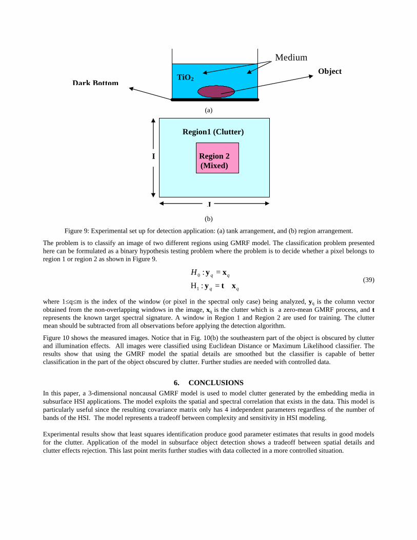
5. APPLICATION: SUBSURFACE OBJECT DETECTION USING HSI Here we show the application of the developed models to subsurface detection of an object embedded in a scattering and absorbing media. Figure 9 shows a schematic of the experimental set up for this application. The object will be immersed in water at six inches mixed with 0.05g of TiO2.

Medium

Dark Bottom Object

TiO2

(a)

Region1 (Clutter)

Region 2 (Mixed)

I

J

(b)

Figure 9: Experimental set up for detection application: (a) tank arrangement, and (b) region arrangement.

The problem is to classify an image of two different regions using GMRF model. The classification problem presented here can be formulated as a binary hypothesis testing problem where the problem is to decide whether a pixel belongs to region 1 or region 2 as shown in Figure 9.

qq

qqH

xty

xy

+=

=

:H

:

1

0 (39)

where 1≤q≤m is the index of the window (or pixel in the spectral only case) being analyzed, yq is the column vector obtained from the non-overlapping windows in the image, xq is the clutter which is a zero-mean GMRF process, and t represents the known target spectral signature. A window in Region 1 and Region 2 are used for training. The clutter mean should be subtracted from all observations before applying the detection algorithm.

Figure 10 shows the measured images. Notice that in Fig. 10(b) the southeastern part of the object is obscured by clutter and illumination effects. All images were classified using Euclidean Distance or Maximum Likelihood classifier. The results show that using the GMRF model the spatial details are smoothed but the classifier is capable of better classification in the part of the object obscured by clutter. Further studies are needed with controlled data.

6. CONCLUSIONS In this paper, a 3-dimensional noncausal GMRF model is used to model clutter generated by the embedding media in subsurface HSI applications. The model exploits the spatial and spectral correlation that exists in the data. This model is particularly useful since the resulting covariance matrix only has 4 independent parameters regardless of the number of bands of the HSI. The model represents a tradeoff between complexity and sensitivity in HSI modeling. Experimental results show that least squares identification produce good parameter estimates that results in good models for the clutter. Application of the model in subsurface object detection shows a tradeoff between spatial details and clutter effects rejection. This last point merits further studies with data collected in a more controlled situation.

(a)

(b)

Figure 10: Measured images (a) Clear water (b) 0.05gr TiO2.

(a)

(b)

Figure 11: Classified image using Euclidean distance (a) MRF-based (b) Spectral only.

(a)

(b)

Figure 12: Classified image using Maximum likelihood classifier: (a) MRF- based (b) Spectral only.

ACKNOWLEDGEMENTS We want to thank Prof. Charles DiMarzio from Northeastern University for providing the HSI data. This work was supported by the US National Science Foundation Engineering Research Centers Program under grant EEC-9986821.

REFERENCES 1. Nemo Program Overview. Downloaded from http://silvereng.com:8080/PDF/NEMO.pdf 2. Susan M. Schweizer and Jose M. F. Moura, “Efficient Detection in Hyperspectral Imagery.” In IEEE Trans. on

Image Processing, Vol. 10(4), pp. 584-597, 2001. 3. Schweizer, S. M., The GMRF Detector for Hyperspectral Imagery: An Efficient Fully-Adaptive Maximum

Likelihood Detector. Ph.D. dissertation, Carnegie Mellon Univ., Pittsburgh, PA, 1999. 4. Susan M. Schweizer and Jose M. F. Moura, “Hyperspectral Imagery: Clutter Adaptation in Anomaly Detection.” In

IEEE Trans. On Information Theory, Vol. 46(5), pp. 1855-1871, 2000. 5. Dimitris Manolakis and Gary Shaw, “Detection Algorithms for Hyperspectral Imaging Applications.” In IEEE

Signal Processing Magazine, Vol. 19(5), pp. 29-43,2002. 6. A. Schaum, “Spectral Subspace Matched Filtering.” In Algorithms for multispectral and Hyperspectral Imagery VII,

Proceedings of SPIE Vol. 4381, pp. 1-17, 2001. 7. Ferrara, Charles F., “Adaptive Spatial/Spectral Detection of Subpixel Targets with Unknown Spectral

Characteristics,” In Signal and Data Processing of Small Targets, Proceedings of SPIE Vol. 2235, pp. 82-93, 1994. 8. Nikhil Balram and Jose M. F. Moura, “Noncausal Gauss Markov Random Fields: Parameter Structure and

Estimation.” In IEEE Trans. On Information Theory, Vol. 39(4), pp. 1333-1355, 1993. 9. Jain, Anil K., Fundamentals of Digital Image Processing. Prentice Hall, Englewood Cliffs, N.J. 569 pp, 1989. 10. Alirez Khotanzad and Jesse Bennett, “A Spatial Correlation Based Method for Neighbor Set Selection in Random

Field Image Models,” In IEEE Trans. on Image Processing, Vol. 8(5), pp. 734-740, 1999. 11. Jose M. F. Moura, and Nikhil Balram, “Recursive Structure of Noncausal Gauss-Markov Random Fields.” In IEEE

Trans. On Information Theory, Vol. 38(2), pp. 334-354,1992. 12. Schott, James R. Matrix Analysis for Statistics. John Wiley & Sons Inc., New York, 1997. 13. Oliver Nelles, Nonlinear System Identification: From Classical Approaches to Neural Networks and Fuzzy Models,

Springer-Verlag, New York, 2001. 14. Luis O. Jimenez, and Jorge Rivera-Medina, “On the Integration of Spatial and Spectral Information in Unsupervised

Classification for Multispectral and Hyperspectral Data.” In Image and Signal Processing for Remote Sensing V, Proceedings of SPIE Vol. 3871, pp. 24-33, 1999.

15. Myers, Raymond H., Classical and Modern Regression with Applications. 2nd ed. Duxbury Thomson Learning, Pacific Grove, CA, 488 pp, 1990.

16. Masalmah, Yahya, Statistical Modeling of Hyperspectral Data using Markov Random Fields, Masters Thesis, University of Puerto Rico at Mayagüez, Mayagüez, PR , June 2002.