Estimating the economic benefits of regional ocean observing systems
132
WHOI-2005-03 Woods Hole Oceanographic Institution o 1- 0/ 1930 Estimating the Economic Benefits of Regional Ocean Observing Systems by Hauke L. Kite-Powell Charles S. Colgan Katharine F. Wellman Thomas Pelsoci Kenneth Wieand Linwood Pendleton Mark J. Kaiser Allan G. Pulsipher Michael Luger April 2005 Technical Report Funding was provided by the Office of Naval Research under Grant No. N00014-02-1-1037. Approved for public release; distribution unlimited.
-
Upload
independent -
Category
Documents
-
view
2 -
download
0
Transcript of Estimating the economic benefits of regional ocean observing systems
WHOI-2005-03
Woods Hole Oceanographic Institution
o 1-
0/
1930
Estimating the Economic Benefits ofRegional Ocean Observing Systems
by
Hauke L. Kite-Powell
Charles S. Colgan
Katharine F. Wellman
Thomas Pelsoci
Kenneth Wieand
Linwood Pendleton
Mark J. Kaiser
Allan G. Pulsipher
Michael Luger
April 2005
Technical Report
Funding was provided by the Office of Naval Research under Grant No. N00014-02-1-1037.
Approved for public release; distribution unlimited.
WHOI-2005-03
Estimating the Economic Benefits ofRegional Ocean Observing Systems
by
Hauke L. Kite-PowellCharles S. Colgan
Katharine F. WellmanThomas PelsociKenneth Wieand
Linwood PendletonMark J. Kaiser
Allan G. PulsipherMichael Luger
April 2005
Technical Report
Funding was provided by the Office of Naval Research under Grant Number N00014-02-1-1037.
Reproduction in whole or in part is permitted for any purpose of the United StatesGovernment. This report should be cited as Woods Hole Oceanog. Inst. Tech. Rept.,
WHOI-2005-03.
Approved for public release; distribution unlimited.
Approved for Distribution:
Andrew Solow, Director
Marine Policy Center
Estimating the Economic Benefits ofRegional Ocean Observing Systems
Report to the National Oceanographic Partnership Program
Marine Policy CenterWoods Hole Oceanographic Institution
May 2005
Hauke L. Kite-Powell,Woods Hole Oceanographic Institution
Charles S. ColganUniversity of Southern MainePrincipal Investigators
Katharine F. WellmanSeattle, WashingtonThomas Pelsoci
Delta Research CompanyKenneth Wieand
University of South FloridaLinwood Pendleton
University of California at Los AngelesMark J. Kaiser and Allan G. Pulsipher
Louisiana State UniversityMichael Luger
University of North Carolina at Chapel Hill
Associate Investigators
20050705 055
Abstract
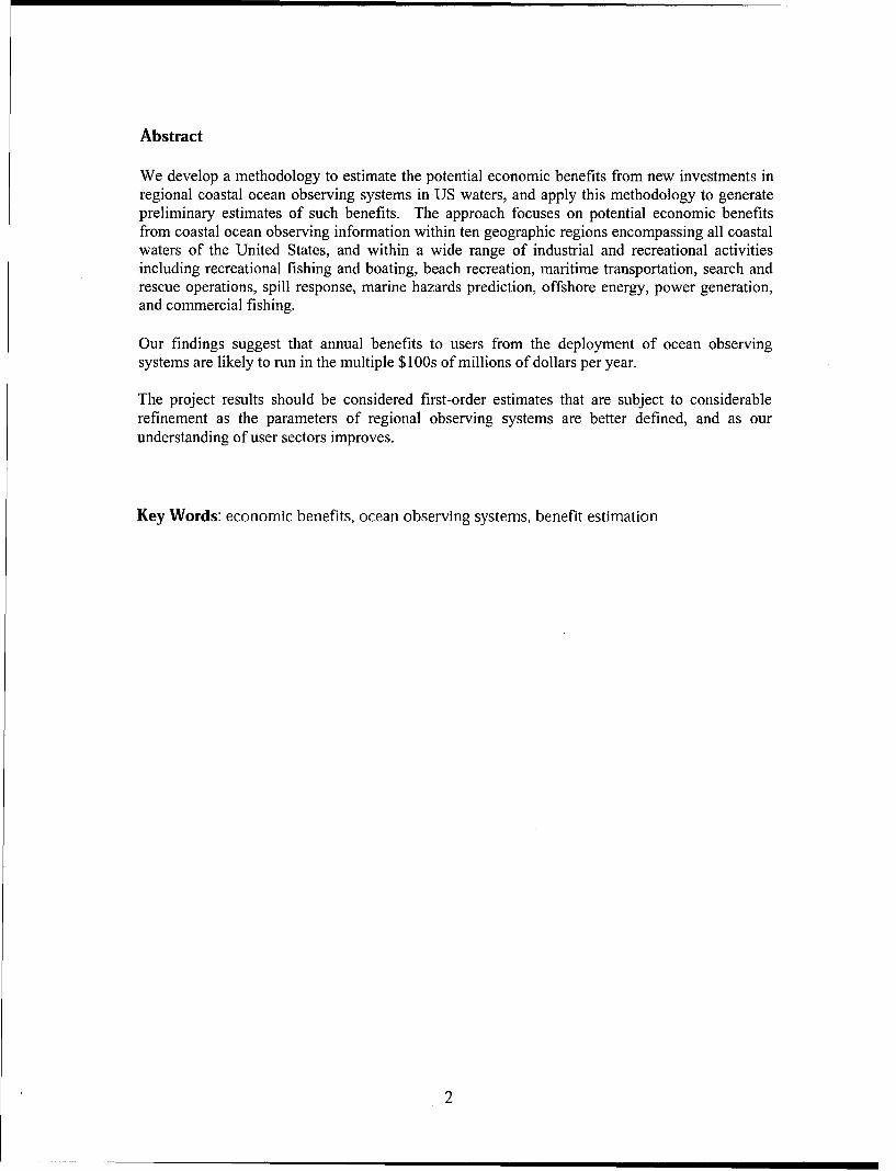
We develop a methodology to estimate the potential economic benefits from new investments inregional coastal ocean observing systems in US waters, and apply this methodology to generatepreliminary estimates of such benefits. The approach focuses on potential economic benefitsfrom coastal ocean observing information within ten geographic regions encompassing all coastalwaters of the United States, and within a wide range of industrial and recreational activitiesincluding recreational fishing and boating, beach recreation, maritime transportation, search andrescue operations, spill response, marine hazards prediction, offshore energy, power generation,and commercial fishing.
Our findings suggest that annual benefits to users from the deployment of ocean observingsystems are likely to run in the multiple $ lOOs of millions of dollars per year.
The project results should be considered first-order estimates that are subject to considerablerefinement as the parameters of regional observing systems are better defined, and as ourunderstanding of user sectors improves.
Key Words: economic benefits, ocean observing systems, benefit estimation
2
Table of Contents
EXECUTIVE SUM M ARY ........................................................................................................................... 5
INTRODUCTION AND SUMMARY ................................................................................................ 15
THE ECONOMIC VALUE OF OCEAN OBSERVING INFORMATION .................................... 19
AN ILLUSTRATIVE EXAMPLE: BEACH CLOSURES AND BEACH USE DECISIONS ..................................... 19
THE ECONOMIC VALUE OF INFORMATION .......................................................................................... 21
Q UANTIFYING ECONOM IC V ALUE ............................................................................................................ 23COMPONENTS OF THE REGIONAL OBSERVING SYSTEMS ........................................................................ 25
ESTIMATES OF POTENTIAL ECONOMIC VALUES OF OBSERVING SYSTEMS ................ 27
CONCLUSIONS AND RECOMMENDATIONS ............................................................................ 35
CO N TRIBU TO RS ..................................................................................................................................... 38
ACKN OW LEDGEM EN TS ....................................................................................................................... 39
APPENDIX A: BEACH MANAGEMENT IN CALIFORNIA ........................................................ 41
APPENDIX B: OFFSHORE ENERGY PRODUCTION IN THE GULF OF MEXICO ............. 61
APPENDIX C: COMMERCIAL FISHERIES IN ALASKA AND THE PACIFIC NORTHWEST.. 89
APPENDIX D: RECREATIONAL BOATING ON THE GREAT LAKES ....................................... 119
3

4
Executive Summary
This report summarizes the findings of a preliminary investigation of the magnitudeof potential economic benefits that can be realized by deploying a network of oceanobserving systems throughout the coastal waters of the United States. Such a network iscurrently being developed through collaborative efforts of federal, state, and localgovernments, universities, and organizations in both the non-profit and for-profit sectors.
Estimating the economic benefits from ocean observing systems is inherentlydifficult. Not only are the systems themselves only partially deployed around the country atpresent; the technology and information products comprising the inputs and outputs of suchsystems are undergoing such rapid evolution that any estimates can only represent a partialsnapshot. Moreover, the economic information needed to compile estimates of both theusers of the information generated by such systems and the value they place on suchinformation is only sporadically available and usually incomplete.
Therefore this report provides what may be considered "order of magnitude"estimates only, along with recommendations on developing more accurate and usefulestimates of economic benefits. Furthermore, there are many possible uses of improvedocean observing systems that have no readily quantifiable economic value but may lead tosignificant benefits in the future. Prominent among these are the uses of better oceanobserving data in a wide range of basic and applied scientific research endeavors and ineducation programs.
The economic benefits of ocean observing systems derive from the value of theinformation generated by such systems and the effects that information has on the behaviorof individuals and organizations. The ideal measure of these economic benefits is the valuethat users of the information place on it, based on their willingness to pay for suchinformation to either enhance their uses of ocean resources or to avoid harms that maycome from oceanic or atmospheric phenomena affecting individuals and organizations. Thewillingness to pay for such information is a measure of what economists call "socialsurplus:" the value of the information in excess of the costs of acquiring it. When suchvalue accrues to businesses, it is referred to as "producer surplus;" when it accrues toindividual users, it is "consumer surplus."
The number of users and types of uses to which the information from oceanobserving systems can be put is large and expanding. A number of uses of ocean observinginformation have been identified to date.' Some of these make use of ocean observing datadirectly, obtaining near-real-time measurements from buoys or other platforms via atelephone or internet interface. Most use the data indirectly, via the output of variousmodels that produce "nowcasts" or forecasts.
See R. Adams, M. Brown, C. Colgan, N. Flemming, H. Kite-Powell, B. McCarl, J. Mjelde, A. Solow, T.Teisberg, and R. Weiher, 2000, The economics of ISOOS: benefits and the rationalefor publicfunding,Washington DC: US Department of Commerce, NOAA Office of Policy and Strategic Planning.
5
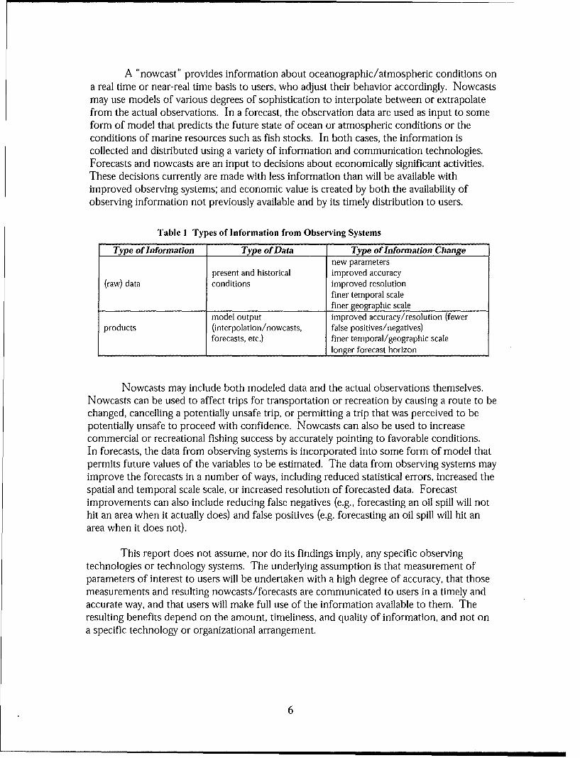
A "nowcast" provides information about oceanographic/atmospheric conditions ona real time or near-real time basis to users, who adjust their behavior accordingly. Nowcastsmay use models of various degrees of sophistication to interpolate between or extrapolatefrom the actual observations. In a forecast, the observation data are used as input to someform of model that predicts the future state of ocean or atmospheric conditions or theconditions of marine resources such as fish stocks. In both cases, the information iscollected and distributed using a variety of information and communication technologies.Forecasts and nowcasts are an input to decisions about economically significant activities.These decisions currently are made with less information than will be available withimproved observing systems; and economic value is created by both the availability ofobserving information not previously available and by its timely distribution to users.
Table I Types of Information from Observing Systems
Type of Information Type of Data Type of Information Changenew parameters
present and historical improved accuracy(raw) data conditions improved resolution
finer temporal scalefiner geographic scale
model output improved accuracy/resolution (fewerproducts (interpolation/nowcasts, false positives/negatives)
forecasts, etc.) finer temporal/geographic scalelonger forecast horizon
Nowcasts may include both modeled data and the actual observations themselves.Nowcasts can be used to affect trips for transportation or recreation by causing a route to bechanged, cancelling a potentially unsafe trip, or permitting a trip that was perceived to bepotentially unsafe to proceed with confidence. Nowcasts can also be used to increasecommercial or recreational fishing success by accurately pointing to favorable conditions.In forecasts, the data from observing systems is incorporated into some form of model thatpermits future values of the variables to be estimated. The data from observing systems mayimprove the forecasts in a number of ways, including reduced statistical errors, increased thespatial and temporal scale scale, or increased resolution of forecasted data. Forecastimprovements can also include reducing false negatives (e.g., forecasting an oil spill will nothit an area when it actually does) and false positives (e.g. forecasting an oil spill will hit anarea when it does not).
This report does not assume, nor do its findings imply, any specific observingtechnologies or technology systems. The underlying assumption is that measurement ofparameters of interest to users will be undertaken with a high degree of accuracy, that thosemeasurements and resulting nowcasts/forecasts are communicated to users in a timely andaccurate way, and that users will make full use of the information available to them. Theresulting benefits depend on the amount, timeliness, and quality of information, and not ona specific technology or organizational arrangement.
6
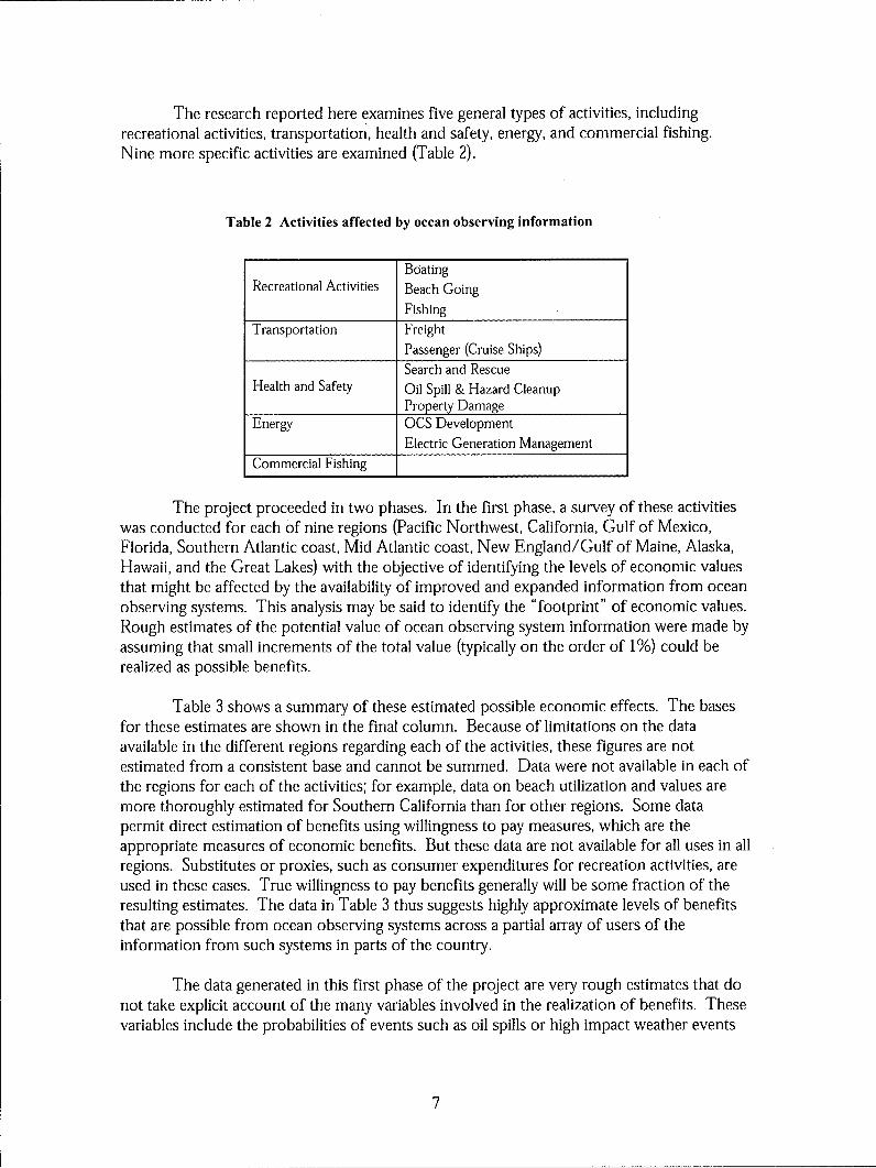
The research reported here examines five general types of activities, includingrecreational activities, transportation, health and safety, energy, and commercial fishing.Nine more specific activities are examined (Table 2).
Table 2 Activities affected by ocean observing information
BoatingRecreational Activities Beach Going
FishingTransportation Freight
Passenger (Cruise Ships)Search and Rescue
Health and Safety Oil Spill & Hazard CleanupProperty Damage
Energy OCS DevelopmentElectric Generation Management
Commercial Fishing
The project proceeded in two phases. In the first phase, a survey of these activitieswas conducted for each of nine regions (Pacific Northwest, California, Gulf of Mexico,Florida, Southern Atlantic coast, Mid Atlantic coast, New England/Gulf of Maine, Alaska,Hawaii, and the Great Lakes) with the objective of identifying the levels of economic valuesthat might be affected by the availability of improved and expanded information from oceanobserving systems. This analysis may be said to identify the "footprint" of economic values.Rough estimates of the potential value of ocean observing system information were made byassuming that small increments of the total value (typically on the order of 1%) could berealized as possible benefits.
Table 3 shows a summary of these estimated possible economic effects. The basesfor these estimates are shown in the final column. Because of limitations on the dataavailable in the different regions regarding each of the activities, these figures are notestimated from a consistent base and cannot be summed. Data were not available in each ofthe regions for each of the activities; for example, data on beach utilization and values aremore thoroughly estimated for Southern California than for other regions. Some datapermit direct estimation of benefits using willingness to pay measures, which are theappropriate measures of economic benefits. But these data are not available for all uses in allregions. Substitutes or proxies, such as consumer expenditures for recreation activities, areused in these cases. True willingness to pay benefits generally will be some fraction of theresulting estimates. The data in Table 3 thus suggests highly approximate levels of benefitsthat are possible from ocean observing systems across a partial array of users of theinformation from such systems in parts of the country.
The data generated in this first phase of the project are very rough estimates that donot take explicit account of the many variables involved in the realization of benefits. Thesevariables include the probabilities of events such as oil spills or high impact weather events
7
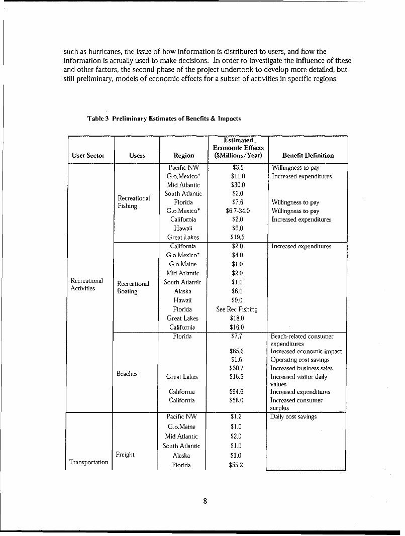
such as hurricanes, the issue of how information is distributed to users, and how theinformation is actually used to make decisions. In order to investigate the influence of theseand other factors, the second phase of the project undertook to develop more detailed, butstill preliminary, models of economic effects for a subset of activities in specific regions.
Table 3 Preliminary Estimates of Benefits & Impacts
EstimatedEconomic Effects
User Sector Users Region ($Millions/Year) Benefit Definition
Pacific NW $3.5 Willingness to payG.o.Mexico* $11.0 Increased expendituresMid Atlantic $30.0
South Atlantic $2.0Fishing Florida $7.6 Willingness to pay
G.o.Mexico* $6.7-34.0 Willingness to pay
California $2.0 Increased expenditures
Hawaii $6.0Great Lakes $19.5California $2.0 Increased expenditures
G.o.Mexico* $4.0G.o.Maine $1.0
Mid Atlantic $2.0Recreational Recreational South Atlantic $1.0Activities Boating Alaska $6.0
Hawaii $9.0
Florida See Rec FishingGreat Lakes $18.0
California $16.0Florida $7.7 Beach-related consumer
expenditures$65.6 Increased economic impact$1.6 Operating cost savings
$30.7 Increased business salesBeaches Great Lakes $16.5 Increased visitor daily
valuesCalifornia $94.6 Increased expendituresCalifornia $58.0 Increased consumer
surplusPacific NW $1.2 Daily cost savings
G.o.Maine $1.0
Mid Atlantic $2.0South Atlantic $1.0
Freight Alaska $1.0Transportation Florida $55.2
8
EstimatedEconomic Effects
User Sector Users Region ($Millions/Year) Benefit Definition
Great Lakes $0.6
California $34.0
G.o.Mexico* $30.7
Cruise Ships Pacific NW $0.1
Pacific NW $10.0 Value of life-$4m
G.o.Maine $24.0Health and Search & Mid Atlantic $16.0Safety Rescue South Atlantic $32.0
California $19.0Alaska $12.0Hawaii $6.0Florida $11.3 Costs saved to USCG plus
Search & value of lost lives savedRescue Florida $22.0 Cost saved to local rescue
squads plus value of lostlives saved.
Great Lakes $18.9 Value of life-$4mG.o.Mexico* $28.0
Health and Oil Spills Pacific NW $0.4 Reductions in clean up andSafety California $0.1 compensation costs
G.o.Mexico* $0.8Tropical South Atlantic $15.6 Reduced loss of life,Storm evacuation cost, and lostPrediction tourism revenueResidential Florida $32.9 Avoided costs from earlierProperty South Atlantic $24.0 preparation for stormsBeach California $1.8 Reduced expenditures onRestoration beach restorationElectric Load Great Lakes $55.8-111.6 Avoided use of mostPlanning expensive peak generatorsOil and Gas G.o.Mexico* $5.1-11.3 Operating cost savings
Energy Development$9-15 Increased accuracy of
oceanographic risks indesign
Pacific NW $2.7 Increased Landed ValuesG.o.Maine $4.0
Mid Atlantic $3.0
Commercial South Atlantic $3.0Alaska $10.0
Fishing Florida $2.0
Great Lakes $0.2 Total regional economicimpact
California $1.2 Reduced operating costsG.o.Mexico* $2.1 Increased Landed Values
*Note that the Gulf of Mexico region in this study excludes the west (Gulf) coast of Florida.
9
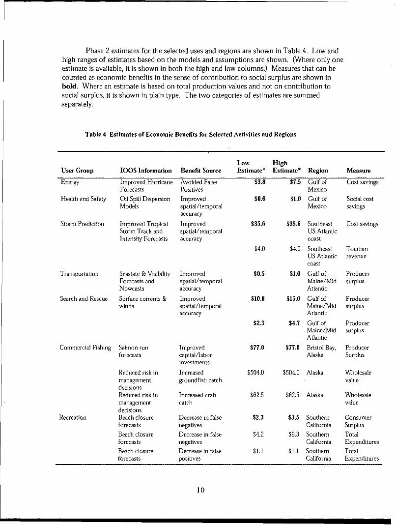
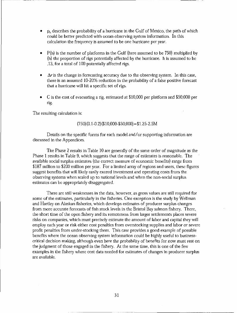
Phase 2 estimates for the selected uses and regions are shown in Table 4. Low andhigh ranges of estimates based on the models and assumptions are shown. (Where only oneestimate is available, it is shown in both the high and low columns.) Measures that can becounted as economic benefits in the sense of contribution to social surplus are shown inbold. Where an estimate is based on total production values and not on contribution tosocial surplus, it is shown in plain type. The two categories of estimates are summedseparately.
Table 4 Estimates of Economic Benefits for Selected Activities and Regions
Low HighUser Group 100S Information Benefit Source Estimate* Estimate* Region Measure
Energy Improved Hurricane Avoided False $3.8 $7.5 Gulf of Cost savingsForecasts Positives Mexico
Health and Safety Oil Spill Dispersion Improved $0.6 $1.0 Gulf of Social costModels spatial/temporal Mexico savings
accuracy
Storm Prediction Improved Tropical Improved $35.6 $35.6 Southeast Cost savingsStorm Track and spatial/temporal US AtlanticIntensity Forecasts accuracy coast
$4.0 $4.0 Southeast TourismUS Atlantic revenuecoast
Transportation Seastate & Visibility Improved $0.5 $1.0 Gulf of ProducerForecasts and spatial/temporal Maine/Mid surplusNowcasts accuracy Atlantic
Search and Rescue Surface currents & Improved $10.0 $15.0 Gulf of Producerwinds spatial/temporal Maine/Mid surplus
accuracy Atlantic
$2.3 $4.7 Gulf of ProducerMaine/Mid surplusAtlantic
Commercial Fishing Salmon run Improved $77.0 $77.0 Bristol Bay, Producerforecasts capital/labor Alaska Surplus
investments
Reduced risk in Increased $504.0 $504.0 Alaska Wholesalemanagement groundfish catch valuedecisionsReduced risk in Increased crab $62.5 $62.5 Alaska Wholesalemanagement catch valuedecisions
Recreation Beach closure Decrease in false $2.3 $3.5 Southern Consumerforecasts negatives California SurplusBeach closure Decrease in false $4.2 $9.3 Southern Totalforecasts negatives California ExpendituresBeach closure Decrease in false $1.1 $1.1 Southern Totalforecasts positives California Expenditures
10
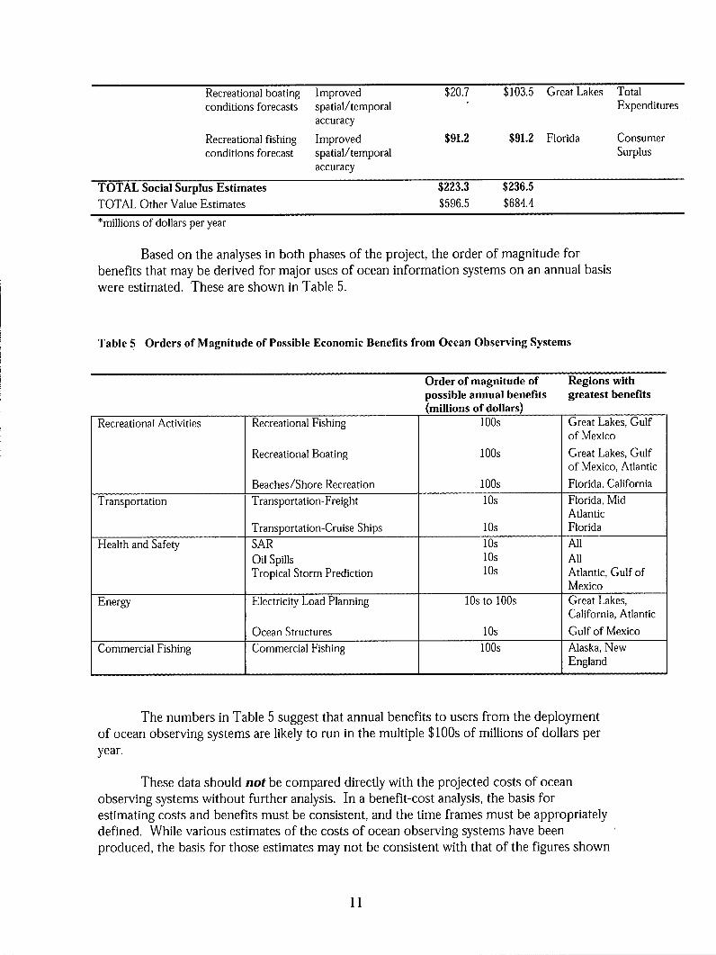
Recreational boating Improved $20.7 $103.5 Great Lakes Totalconditions forecasts spatial/temporal Expenditures
accuracy
Recreational fishing Improved $91.2 $91.2 Florida Consumerconditions forecast spatial/temporal Surplus
accuracy
TOTAL Social Surplus Estimates $223.3 $236.5TOTAL Other Value Estimates $596.5 $684.4*millions of dollars per year
Based on the analyses in both phases of the project, the order of magnitude forbenefits that may be derived for major uses of ocean information systems on an annual basiswere estimated. These are shown in Table 5.
Table 5 Orders of Magnitude of Possible Economic Benefits from Ocean Observing Systems
Order of magnitude of Regions withpossible annual benefits greatest benefits(millions of dollars)
Recreational Activities Recreational Fishing 100s Great Lakes, Gulfof Mexico
Recreational Boating 100s Great Lakes, Gulfof Mexico, Atlantic
Beaches/Shore Recreation loos Florida, California
Transportation Transportation-Freight los Florida, MidAtlantic
Transportation-Cruise Ships los Florida
Health and Safety SAR los All
Oil Spills los AllTropical Storm Prediction los Atlantic, Gulf of
MexicoEnergy Electricity Load Planning 1Os to 100s Great Lakes,
California, Atlantic
Ocean Structures los Gulf of MexicoCommercial Fishing Commercial Fishing loos Alaska, New
England
The numbers in Table 5 suggest that annual benefits to users from the deploymentof ocean observing systems are likely to run in the multiple $100s of millions of dollars peryear.
These data should not be compared directly with the projected costs of oceanobserving systems without further analysis. In a benefit-cost analysis, the basis forestimating costs and benefits must be consistent, and the time frames must be appropriatelydefined. While various estimates of the costs of ocean observing systems have beenproduced, the basis for those estimates may not be consistent with that of the figures shown
11
in this report. At this stage, our findings are also not precise enough to be used to conductbenefit-cost analyses of specific technologies or specific regions.
However, we can conclude from these data that on a discounted present value basisover time2 , the benefits from a national investment in such systems are likely to exceed thecosts. This finding is consistent with previous conclusions on the economic benefits of suchsystems (see, for example, the report cited in Footnote 1 above).
The data also indicate that ocean observing systems will have the largest benefitswhere the information from such systems is used by the largest possible groups.Recreational activities are consistently the highest generators of benefits because of the verylarge number of people who use beaches, boat on the Great Lakes or in the coastal ocean, orengage in marine recreational fishing. Although the per-user benefits are smaller than thoserealized by other activities, the large number of users drive the overall magnitude of potentialbenefits to substantial sums.
Several important caveats are required in interpreting the results presented above:
" The fact that the benefits from the systems as a whole will likely exceed the costsdoes not mean that the benefits will exceed the costs in every individual case. Theconfiguration of observing systems in each region should take into account thepriorities of local and regional user groups.
The estimates presented assume:
"* Full and successful deployment of existing, near-deployment, or reasonablyforseeable technologies.
"• Cost efficient and effective means of communicating the information derived fromthe ocean observations to users in a timely manner.
"* Users are aware of, and effectively incorporate, the information into decisionsregarding their activities.
"* In the case of commercial fisheries, additional information concerning the state ofthe marine environment is relevant to decisions about managed fisheries and (atsome point) will permit increases in allowable catches.
Violation of any of these assumptions may reduce the potential or actual benefits to levelsbelow those estimated here.
The analysis of economic benefits from ocean observing systems in this study is byno means exhaustive. For example, this study does not address benefits that may arise forthe hotel and resort industry or for certain aspects of emergency management. One source
2 "Discounted present value" is a means of adding benefits (or costs) that accrue at different points in time
to obtain a meaningful single value. A discount rate is applied to convert benefits (or costs) that arise infuture years into "present" dollars. This is necessary because (a) the value of a dollar next year is (usually)less than the value of a dollar today, and (b) there is (generally) greater uncertainty about benefits (or costs)expected to arise in future years.
12
of complementary information about benefits in these and other areas is a series of reportsprepared for NOAA by SAIC Inc. (http://www.saic.com/weather/papers.html).
Based on these findings, we believe additional research is needed to develop moreprecise estimates of benefits for specific observing systems, instruments, technologies, andapplications. Specifically:
1. Operators of regional observing systems should incorporate in their operationalplans strategies and activities to measure the economic benefits of their products andservices.
2. Investments should be made by federal, state, and local governments in moreprecisely estimating economic benefits and in sharing data and methods for benefitsestimation among operators of observing systems. To build on the work presentedin this report, a series of coordinated pilot projects should be funded at the regionallevel to develop, apply, and share with other regions detailed guidelines for benefittracking and estimation. These pilot projects should focus on one or two prominentuser sectors in each region, and cover the major sectors identified in this report.
3. Consumer surplus benefits should be estimated for all categories of recreation usersin various regions of the country. Current estimates of such benefits do not fullyaccount for the possibility of substitution among different recreation resources indifferent regions and remain subject to considerable methodological variability.
13

14
Introduction and Summary
The United States and other countries are designing and building a large network ofinstrumentation and data links to continuously monitor biological, physical, and chemicalconditions in the ocean and in the ocean-atmosphere interface. This network will extendfrom the near shore areas of America's ocean and Great Lakes coasts (and those of othercountries) to the deep ocean areas.
The expansion of ocean observing systems is made possible by innovations insensor, computer, and communication technologies that have lowered the cost ofinstrumentation and made it possible to measure more parameters than ever before. Thepresence of data distribution technologies such as the Internet have also enhanced the valueand cost-effectiveness of such systems, because data can now be delivered directly topotential users at very low or no cost.
While the costs of collecting and distributing data from ocean observingtechnologies have come down on a per unit basis, the creation of the systems of observingtechnologies still requires significant investments. Those investments will be made byfederal, state, and local governments and by other organization in both the private profit andnon-profit sectors. The magnitude of investments required raises questions about what thebenefits from such systems will be, and whether these will be sufficient to warrant therequired investments.
This report presents preliminary information about the magnitude of likely benefitsthat may accrue from current and expected regional observing systems. The focus is onobserving systems to be deployed in the coastal waters of the United States, including boththe oceans and the Great Lakes. These observing systems are being formed as a series ofregional systems in areas such as the Gulf of Maine, South Atlantic, California, Gulf ofMexico, Pacific Northwest, and Gulf of Alaska. It is anticipated that all of the coastal watersof the United States eventually will be covered by such systems, which will provide nationallyconsistent measurement of certain parameters (the "national backbone") and also meetparticular needs in each region. Output from the network of regional systems will merge toprovide an integrated ocean observing system for the United States, which in turn will be acomponent of the Global Ocean Observing System (GOOS) and the Global EarthObserving System (GEOS). For more information about the network of regional observingsystems see www.ocean.us.
The information needed to develop detailed estimates of the economic benefits ofocean observing systems is, for the most part, unavailable at this time. Both thedevelopment of the observing systems themselves and the economic information needed toestimate benefits are presently incomplete. The analysis developed here therefore attemptsto identify likely magnitude of benefits based on the levels of economic activity potentiallyaffected by the information derived from ocean observations, and to explore the methodsthat can be used to develop detailed estimates for specific applications in selected regions.
15
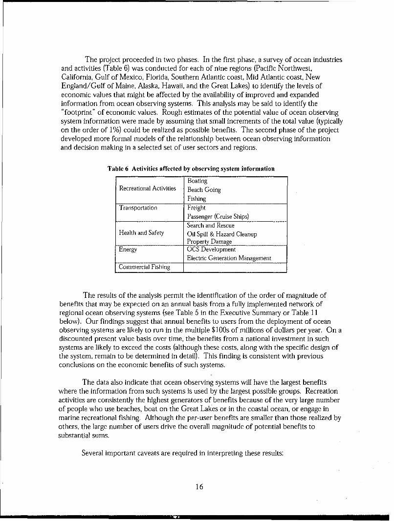
The project proceeded in two phases. In the first phase, a survey of ocean industriesand activities (Table 6) was conducted for each of nine regions (Pacific Northwest,California, Gulf of Mexico, Florida, Southern Atlantic coast, Mid Atlantic coast, NewEngland/Gulf of Maine, Alaska, Hawaii, and the Great Lakes) to identify the levels ofeconomic values that might be affected by the availability of improved and expandedinformation from ocean observing systems. This analysis may be said to identify the"footprint" of economic values. Rough estimates of the potential value of ocean observingsystem information were made by assuming that small increments of the total value (typicallyon the order of 1%) could be realized as possible benefits. The second phase of the projectdeveloped more formal models of the relationship between ocean observing informationand decision making in a selected set of user sectors and regions.
Table 6 Activities affected by observing system information
BoatingRecreational Activities Beach Going
FishingTransportation Freight
Passenger (Cruise Ships)Search and Rescue
Health and Safety Oil Spill & Hazard CleanupProperty Damage
Energy OCS DevelopmentElectric Generation Management
Commercial Fishing I
The results of the analysis permit the identification of the order of magnitude ofbenefits that may be expected on an annual basis from a fully implemented network ofregional ocean observing systems (see Table 5 in the Executive Summary or Table 11below). Our findings suggest that annual benefits to users from the deployment of oceanobserving systems are likely to run in the multiple $100s of millions of dollars per year. On adiscounted present value basis over time, the benefits from a national investment in suchsystems are likely to exceed the costs (although these costs, along with the specific design ofthe system, remain to be determined in detail). This finding is consistent with previousconclusions on the economic benefits of such systems.
The data also indicate that ocean observing systems will have the largest benefitswhere the information from such systems is used by the largest possible groups. Recreationactivities are consistently the highest generators of benefits because of the very large numberof people who use beaches, boat on the Great Lakes or in the coastal ocean, or engage inmarine recreational fishing. Although the per-user benefits are smaller than those realized byothers, the large number of users drive the overall magnitude of potential benefits tosubstantial sums.
Several important caveats are required in interpreting these results:
16

"* The fact that the benefits from the systems as a whole will exceed the costs does notmean that the benefits will exceed the costs in every individual case. Theconfiguration of observing systems in each region should take into account thepriorities of local and regional user groups.
The estimates presented assume:
"* Full and successful deployment of existing or near-deployment technologies."• Cost efficient and effective means of communicating the information derived from
the ocean observations to users in a timely manner."• Users are aware of, and effectively incorporate, the information into their decisions
regarding their activities"* In the case of commercial fisheries, additional information concerning the state of
the marine environment is relevant to decisions about managed fisheries and (atsome point) will permit increases in allowable catches.
Violation of any of these assumptions may reduce the possible or actual benefits to levelsbelow those estimated here.
The following sections of the report discuss the derivation of these estimates. In thenext section, the general theory of economic benefits is discussed, along with a generalintroduction to ocean observing technologies and their information products. The followingtwo sections discuss the details of estimating procedures in the two phases of the project.The final section provides conclusions and recommendations.
Selected individual reports from Phase 2 of the project are included in theAppendices.
17

18
The Economic Value of Ocean Observing Information
The information derived from ocean observing systems creates economic valueprimarily by leading to improved decision making. "Improvement" in this context meansreducing the uncertainty associated with actions taken to use marine resources in some way.A large degree of uncertainty surrounds such decisions; and much of this uncertainty existsbecause the person facing a decision does not have complete information about the relevantstate of the ocean at the relevant time. Ocean observing data and the information derivedfrom them reduce this uncertainty, and that reduction in uncertainty is economicallyvaluable. What a decision maker should be willing to pay for this information (the marketvalue of the information) is related to the extent to which it reduces uncertainty, and to theeconomic resources at stake in the decision.
An Illustrative Example: Beach Closures and Beach Use Decisions
This definition of the value of information provides the elements necessary toestimate the value of ocean observing (or other) information. Consider the followingexample:
A surfer in Southern California wants to go to the beach for a day's surfing, but herdecision to actually go depends on knowing whether the beach is open for swimming andwhat is the current state of the surf. General weather forecasts are available, as isinformation about whether the beach is closed or not. (Beach closures usually follow fromsewage overflows that may increase the presence of pathogenic bacteria in the water.)
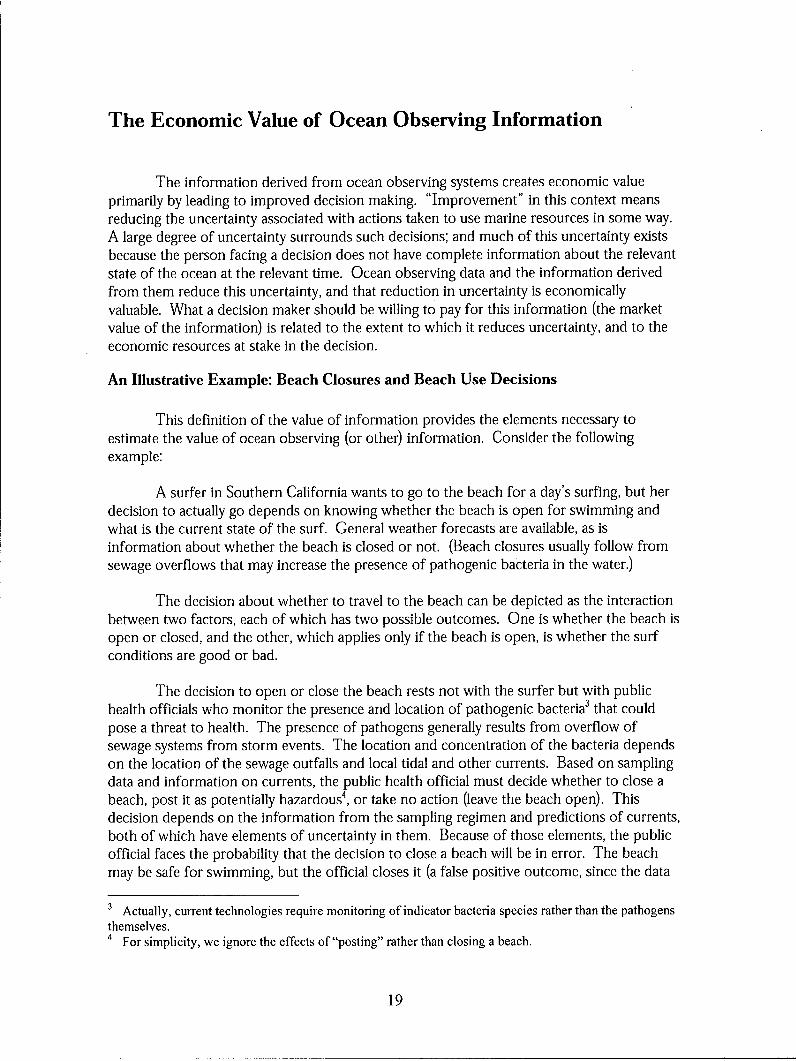
The decision about whether to travel to the beach can be depicted as the interactionbetween two factors, each of which has two possible outcomes. One is whether the beach isopen or closed, and the other, which applies only if the beach is open, is whether the surfconditions are good or bad.
The decision to open or close the beach rests not with the surfer but with publichealth officials who monitor the presence and location of pathogenic bacteria3 that couldpose a threat to health. The presence of pathogens generally results from overflow ofsewage systems from storm events. The location and concentration of the bacteria dependson the location of the sewage outfalls and local tidal and other currents. Based on samplingdata and information on currents, the public health official must decide whether to close abeach, post it as potentially hazardous 4, or take no action (leave the beach open). Thisdecision depends on the information from the sampling regimen and predictions of currents,both of which have elements of uncertainty in them. Because of those elements, the publicofficial faces the probability that the decision to close a beach will be in error. The beachmay be safe for swimming, but the official closes it (a false positive outcome, since the data
3 Actually, current technologies require monitoring of indicator bacteria species rather than the pathogensthemselves.4 For simplicity, we ignore the effects of "posting" rather than closing a beach.
19
indicates a positive result for pathogenic exposure, leading to a closure decision). Or thebeach may actually be unsafe for swimming and kept open in error (a false negativeoutcome). Since the official is likely to be risk averse, more beaches are likely to be closedwhen they could be open if uncertainty were reduced.
GoodConditions
Beach
Figure 1 Decision to Surf
The decision to open or close the beach is influenced strongly by knowledge of localconditions in the vicinity of sewage outfalls and storm drains. Ocean observing system canprovide fine scale (both temporal and spatial) information on physical, chemical, andbiological conditions, and thereby significantly alter the public health official's decisionproblem. By reducing uncertainty, the length of beaches that must be closed can be reduced,as can the risk of false positives or false negatives. A reduction in false positives increasesthe amount of time beaches are open for recreation, while a reduction in false negativesdecreases the risks to swimmers' and surfers' health and safety.
For the surfer, the question of conditions is a subjective one that depends on windand wave conditions, which may be unique to the particular destination beach. Again, finertemporal and spatial scale oceanographic and meteorological information provides theinformation the surfer needs to decide whether to make the trip to the beach.
The economic value at stake in these decisions is the value received from safelyenjoying the recreational activity. That value is the amount the surfer would be willing topay for the opportunity to go surfing less the amount that is actually paid (usually
20
transportation costs). If the surfer makes the trip only to find the beach closed or to findsurf conditions too large or too small for enjoyable surfing, then there is a loss of value. Itis thus the value to the surfer (or other recreationist) that is at stake in this use of the oceanobserving system information. The reduction in uncertainty for the public health officialcreates value to the extent that it increases the value of recreation to those who use thebeach.
This example illustrates the two most fundamental ways that ocean observingsystems information is used: to create forecasts of future information on which decisionsdepend, and to create nowcasts of conditions in real or near-real time. Forecasts aregenerated when data from observing systems are fed into models of ocean and atmosphericprocesses to generate the required information. Nowcast information may be directobservation data (wind speed, wave height) or may also be produced by models. Theseeffects are summarized in Table 7.
Table 7 Ocean observing information uses
Type of Type of Data Type of InformationInformation ChangeForecasts Modeled data Forecast Accuracy
Spatial ScaleTemporal ScaleAvoiding False NegativesAvoiding False Positives
Nowcasts Observation data Transportation routingModeled data Fishing success
The Economic Value of Information
As the surfer example illustrates, a nowcast or forecast based on ocean observingsystem data represents information about conditions or phenomena in the ocean. Thisinformation has value when it can be used by an individual or an organization to make abetter decision - that is, a decision that results in an outcome that is economically superior.The standard economic approach to valuing information requires:
"* A description of the information being valued (in this case, typically an improvedforecast or nowcast) and of the uncertainty in the phenomena is describes.
" A model of how this information is used to make decisions. Most decisions aremade in the face of imperfect information, or uncertainty about how conditions willin fact develop and what the exact outcome will be. Therefore, a basic principle ofeconomic valuation of information is that of "expected values." Expected values aredefined as values adjusted for the probability that they will be realized. In theabsence of a specific model of decision behavior, it makes sense to assume thedecision maker is rational and seeks to maximize benefits. This is described ingreater detail below.
21
"* A model of how these decisions affect physical outcomes.
" A model of how physical outcomes can be translated into economic outcomes. Thevalue of a forecast is the difference between the expected value of the outcome ofdecisions using the forecast, and the expected value of the outcome without theforecast.
A standard Bayesian approach can be used to estimate the value of informationcontained in a forecast (see Berger 1995).5 In this model, a decision maker (user offorecasts) must choose among a range of actions represented by A. The outcome of eachaction depends on a state of nature, S, which is not known at the time of the decision butbecomes manifest later. The manifestation of S is modeled as a random variable withprobability density function f(s). This probability density function (pdf) describes theprobability that the condition (for example, the height of waves at a surfing beach) will liewithin a particular range considering only what is known from past observation, anddisregarding the new forecast.
Let B(a,s) be the consequence (net benefit) to the decision maker of pursuing action aif it turns out that S=s. The expected net benefit of pursuing action a is then the integral ofthe product of B(a,s) and f(s) (see Raiffa 1970):6
E = f B(a, s)f(s)ds
The optimal choice of action without the new forecast (a0* is that which produces themaximum expected net benefit (E0). If we now provide a useful new forecast to thedecision maker, the optimal choice of action and the associated expected net benefit willchange. To determine the value of this new forecast, we need to know something about theaccuracy of this forecast and something about the frequency with which different conditionsarise on average. (For instance, a storm forecast may be more valuable if storms are morefrequent than if they only happen once a decade.) How a decision maker revises herestimate of the likelihood of s is described by Bayes' Theorem:
f (s I x) = l(x s)f (s) / p(x)
where X is the information in the forecast,1(x/s) is the probability that X =x given S=s, andp(x) is the probability that X=x:
p(x) = l(x I s)f (s)ds
5 Berger, J.O. 1985. Statistical decision theory and Bayesian analysis. New York, Springer Verlag.6 Raiffa, Howard. 1970. Decision Analysis: Introductory Lectures on Choices under Uncertainty.
Boston: Addison Wesley.
22
In simple terms, Bayes' Theorem describes how the decision maker should adjust her priorexpectation of the occurrence of event s when the forecast says x, taking into account how"good" this forecast tends to be.
The new optimal action given forecast X is found be maximizing
E (aIx) = J B(a,s)f(s I x)ds
The outcome of the optimal choice, E*(x), now depends on x, and the expected value of netbenefit is
E f E * (x)p(x)dx
Since the decision maker could realize expected benefit Eo* without the forecast and Ex*with the forecast, the value of this forecast to the decision maker is Ex* - Eo*.
In this description of the theoretical underpinning of the value of information, wehave not addressed the question of how the net benefit (E) is quantified in each case. Weturn to this question in the following section.
Quantifying Economic Value
The information uses outlined in the example of the surfer can be extended to manydifferent types of users. Recreational boaters and those who fish in marine waters havesimilar needs for fine scale oceanographic and meteorological data to decide when andwhere to go. Cargo and cruise ships, both sensitive to fuel costs, need real time currentinformation to optimize their routes to and from harbors; and tug/barges and pilot boats areinterested in wave height information to avoid hazardous operating conditions. Commercialfishermen have similar needs; and both recreational and commercial fishing success can beimproved by knowledge of such parameters as water temperature. Electric generators canoptimize fuel generation to minimize costs depending on when the sea breeze sets up on ahigh demand summer afternoon, while offshore oil and gas operators need information onhigh velocity loop currents that develop in the Gulf of Mexico and can affect the safety ofoperations. With accurate surface current information, oil spill response teams can moreeffectively deploy equipment to where the oil will be and avoid where the oil will not be.
The appropriate measure of economic value in all of these cases is the change inwhat economists refer to as "social surplus." Social surplus has two components: producersurplus and consumer surplus. Producer surplus in this case is generally the differencebetween the costs incurred by businesses (including opportunity costs, or reasonable rates ofreturn on inputs to production) and the revenues they realize. Consumer surplus, as in thecase of the surfer, is the difference between what one would be willing to pay and what oneactually pays for, for example, a recreational experience. "Social surplus" is the sum ofproducer and consumer surplus. Social surplus is the best single measure of economic
23
benefits because it assures that only value in excess of costs is included, and avoids theartificial inflation of values caused by double counting.
The problem with social surplus and both of its compoents is that they can only bemeasured using exacting, time-consuming, and costly techniques. Other measures ofeconomic activity (broadly termed "economic impacts"), such as the value of sales at thewholesale or retail level, or value added (the most common example of which is the GrossDomestic Product), are widely available, but measure social surplus only in an imperfectmanner.
Studies of economic values from investments such as ocean observing systems thusface a dilemma. The most appropriate measure is the least readily available, while the mostavailable measures are the least appropriate. This is a major reason why estimates ofeconomic benefits from ocean observing activities at this stage of analysis must beconsidered preliminary and approximate. In this study, most of the estimates have beendeveloped using an indirect and somewhat restrictive approach.
The first step is to identify some of the activities that could be affected by oceanobserving systems, and to obtain data from public statistical sources that indicateapproximate levels of economic activity in these areas. Simple assumptions are then madeabout the possible level of benefits from improved information. In most cases, socialsurplus benefits are assumed to be no more than 1% of total activity values; this is aconservative assumption which reflects the reality that changes in producer and consumersurplus are likely to small relative to aggregate expenditure or sales data.7
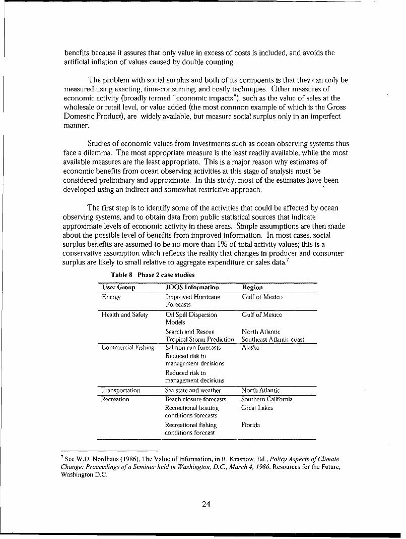
Table 8 Phase 2 case studies
User Group IOOS Information RegionEnergy Improved Hurricane Gulf of Mexico
Forecasts
Health and Safety Oil Spill Dispersion Gulf of MexicoModelsSearch and Rescue North AtlanticTropical Storm Prediction Southeast Atlantic coast
Commercial Fishing Salmon run forecasts AlaskaReduced risk inmanagement decisionsReduced risk inmanagement decisions
Transportation Sea state and weather North AtlanticRecreation Beach closure forecasts Southern California
Recreational boating Great Lakesconditions forecasts
Recreational fishing Floridaconditions forecast
7 See W.D. Nordhaus (1986), The Value of Information, in R. Krasnow, Ed., Policy Aspects of ClimateChange: Proceedings of a Seminar held in Washington, D.C., March 4, 1986. Resources for the Future,Washington D.C.
24
In order to test methods for more precise estimates of social surplus, case studieswere undertaken as a second step in this study. These case studies are shown in Table 8 anddiscussed in a subsequent section of this report.
Components of the regional observing systems
Before proceeding to a discussion of economic values, it is necessary to discussbriefly the assumptions used in this study about ocean observing systems. Team membersconsulted widely with organizations and scientists currently designing and operatingobserving systems in the coastal waters of the U.S., including the Great Lakes. The teamalso received valuable guidance from the U.S. Global Ocean Observing Systems SteeringCommittee.
The technologies comprising ocean observing systems include a wide array ofinstruments and platforms. They include moored and unmoored buoys, radar, satelliteimagery, fixed platforms such as light stations, and platforms of opportunity. Satellites,moored buoys, and radar make up much of the current generation of improvements inocean observing systems. The data output from these instruments consist of a wide array ofparameters, including:
"* Wind speed and direction"* Current speed and direction"* Wave height and periodicity"* Air and water temperature at varying heights/depths"* Chemical composition such as salinity"* Biological composition, particularly the density of chlorophyll-A"* Visibility"• Ice (Great Lakes)
The data derived from these observations are distributed directly and indirectlythrough a variety of means. The data may be fed to forecasting centers operated by thefederal government, universities, or private organizations for incorporation into forecastproducts that are distributed widely through public and private channels including television,newspapers, radio, or the Internet. The data may also be delivered directly to subscribers.
In conducting the analysis for this project, no attempt was made to evaluate thebenefits of specific technologies, instruments, platforms, or communication channels. Theassumption was made that economically-relevant data would be available in an integratedform and timely manner to users irrespective of observation technology or datadissemination means.
In general, we assumed the sort of data and information streams that are alreadybeing delivered by one or more of the ocean observing system organizations. We made nospecific assumptions about improvements in data other than that development of the
25
observing technologies and systems would permit a substantial increase in the amount,quality, and usability of information delivered to users. In some cases, such as thedevelopment of methods for more rapid and direct measurement of pathogenic bacteria, wehave assumed that such developments will take place and be implemented (we include theuse of rapid microbial indicators as one type of instrumentation that could produce data onbiological pathogens).
In short, we have assumed that when users need information, it will be available andfully utilized (incorporated into relevant decisions). The benefits shown are thus potentialbenefits from systems being established and expanded, not from the array of observingtechnologies, platforms, and data distribution in place at the time of this study.
26
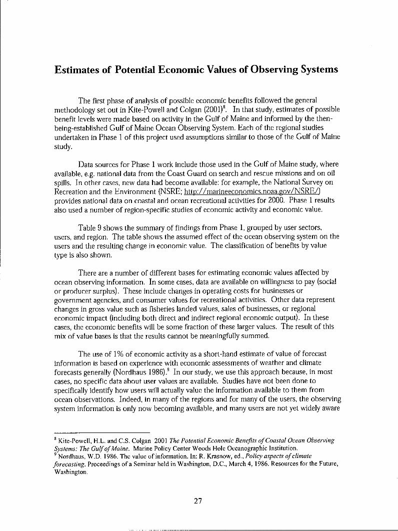
Estimates of Potential Economic Values of Observing Systems
The first phase of analysis of possible economic benefits followed the generalmethodology set out in Kite-Powell and Colgan (2001)8. In that study, estimates of possiblebenefit levels were made based on activity in the Gulf of Maine and informed by the then-being-established Gulf of Maine Ocean Observing System. Each of the regional studiesundertaken in Phase 1 of this project used assumptions similar to those of the Gulf of Mainestudy.
Data sources for Phase 1 work include those used in the Gulf of Maine study, whereavailable, e.g. national data from the Coast Guard on search and rescue missions and on oilspills. In other cases, new data had become available: for example, the National Survey onRecreation and the Environment (NSRE; http://marineeconomics.noaa.gov/NSRE/)provides national data on coastal and ocean recreational activities for 2000. Phase 1 resultsalso used a number of region-specific studies of economic activity and economic value.
Table 9 shows the summary of findings from Phase 1, grouped by user sectors,users, and region. The table shows the assumed effect of the ocean observing system on theusers and the resulting change in economic value. The classification of benefits by valuetype is also shown.
There are a number of different bases for estimating economic values affected by
ocean observing information. In some cases, data are available on willingness to pay (socialor producer surplus). These include changes in operating costs for businesses orgovernment agencies, and consumer values for recreational activities. Other data representchanges in gross value such as fisheries landed values, sales of businesses, or regionaleconomic impact (including both direct and indirect regional economic output). In thesecases, the economic benefits will be some fraction of these larger values. The result of thismix of value bases is that the results cannot be meaningfully summed.
The use of 1% of economic activity as a short-hand estimate of value of forecastinformation is based on experience with economic assessments of weather and climateforecasts generally (Nordhaus 1986).' In our study, we use this approach because, in mostcases, no specific data about user values are available. Studies have not been done tospecifically identify how users will actually value the information available to them fromocean observations. Indeed, in many of the regions and for many of the users, the observingsystem information is only now becoming available, and many users are not yet widely aware
8 Kite-Powell, H.L. and C.S. Colgan 2001 The Potential Economic Benefits of Coastal Ocean Observing
Systems: The Gulf of Maine. Marine Policy Center Woods Hole Oceanographic Institution.9 Nordhaus, W.D. 1986. The value of information. In: R. Krasnow, ed., Policy aspects of climateforecasting. Proceedings of a Seminar held in Washington, D.C., March 4, 1986. Resources for the Future,Washington.
27
of the availability of such information, nor have users (and economists) gained theexperience with the data to develop meaningful "willingness to pay" values.
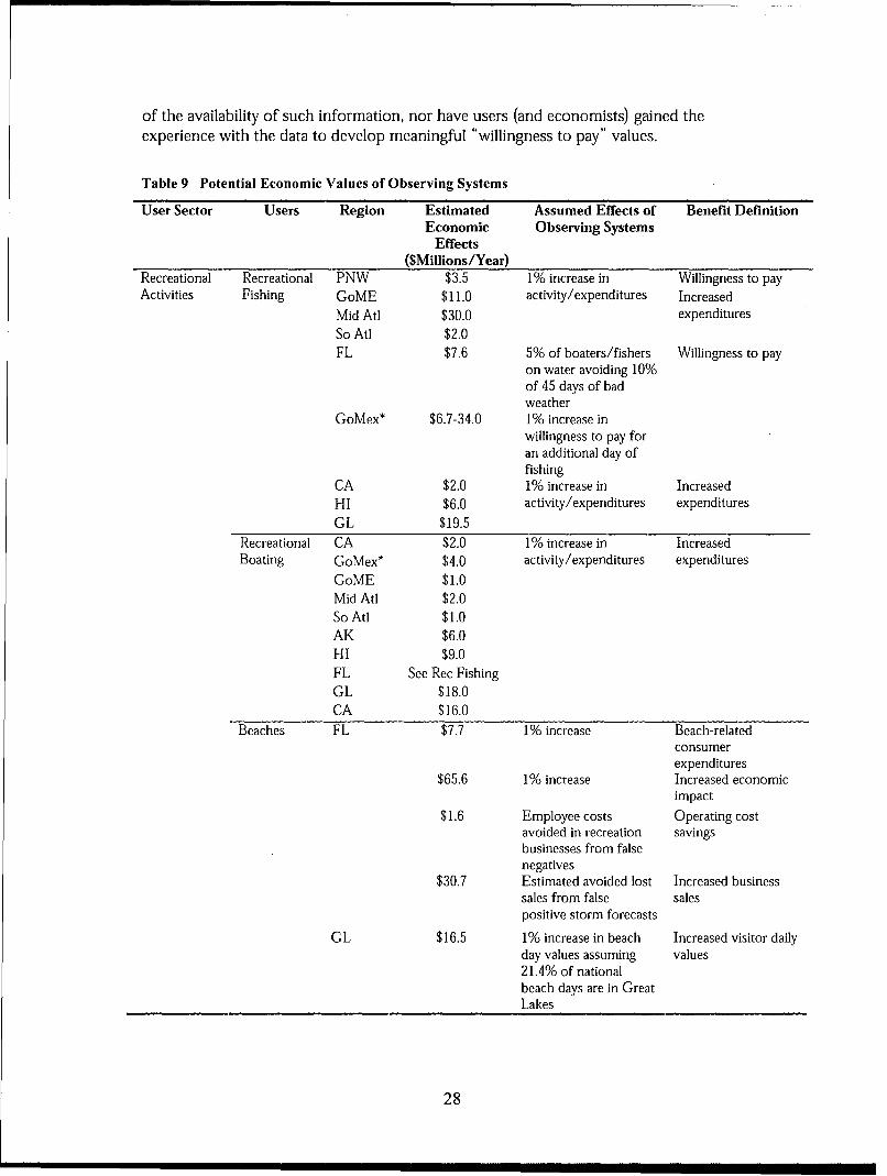
Table 9 Potential Economic Values of Observing Systems
User Sector Users Region Estimated Assumed Effects of Benefit DefinitionEconomic Observing Systems
Effects($Millions/Year)
Recreational Recreational PNW $3.5 1% increase in Willingness to payActivities Fishing GoME $11.0 activity/expenditures Increased
Mid At] $30.0 expendituresSo Ati $2.0FL $7.6 5% of boaters/fishers Willingness to pay
on water avoiding 10%of 45 days of badweather
GoMex* $6.7-34.0 1% increase inwillingness to pay foran additional day offishing
CA $2.0 1% increase in IncreasedHI $6.0 activity/expenditures expendituresGL $19.5
Recreational CA $2.0 1% increase in IncreasedBoating GoMex* $4.0 activity/expenditures expenditures
GoME $1.0Mid AtI $2.0So Ati $1.0AK $6.0HI $9.0FL See Rec FishingGL $18.0CA $16.0
Beaches FL $7.7 1% increase Beach-relatedconsumerexpenditures
$65.6 1% increase Increased economicimpact
$1.6 Employee costs Operating costavoided in recreation savingsbusinesses from falsenegatives
$30.7 Estimated avoided lost Increased businesssales from false salespositive storm forecasts
GL $16.5 1% increase in beach Increased visitor dailyday values assuming values21.4% of nationalbeach days are in GreatLakes
28
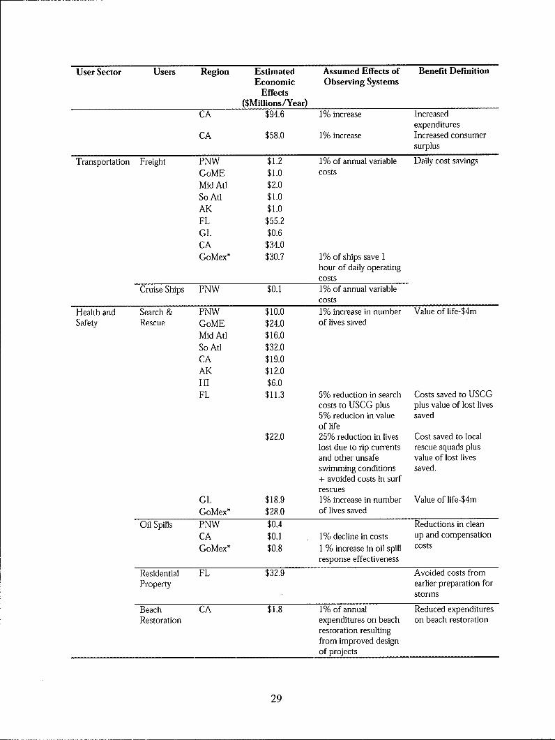
User Sector Users Region Estimated Assumed Effects of Benefit DefinitionEconomic Observing Systems
Effects($Millions/Year)
CA $94.6 1% increase Increasedexpenditures
CA $58.0 1% increase Increased consumersurplus
Transportation Freight PNW $1.2 1% of annual variable Daily cost savingsGoME $1.0 costs
Mid At] $2.0So At $1.0AK $1.0FL $55.2GL $0.6CA $34.0GoMex* $30.7 1% of ships save 1
hour of daily operatingcosts
Cruise Ships PNW $0.1 1% of annual variablecosts
Health and Search & PNW $10.0 1% increase in number Value of life-$4mSafety Rescue GoME $24.0 of lives saved
Mid Ati $16.0So Ati $32.0CA $19.0AK $12.0HI $6.0FL $11.3 5% reduction in search Costs saved to USCG
costs to USCG plus plus value of lost lives5% reducion in value savedof life
$22.0 25% reduction in lives Cost saved to locallost due to rip currents rescue squads plusand other unsafe value of lost livesswimming conditions saved.+ avoided costs in surfrescues
GL $18.9 1% increase in number Value of life-$4mGoMex* $28.0 of lives saved
Oil Spills PNW $0.4 Reductions in cleanCA $0.1 1% decline in costs up and compensation
GoMex* $0.8 1 % increase in oil spill costs
response effectiveness
Residential FL $32.9 Avoided costs fromProperty earlier preparation for
storms
Beach CA $1.8 1% of annual Reduced expendituresRestoration expenditures on beach on beach restoration
restoration resultingfrom improved designof projects
29
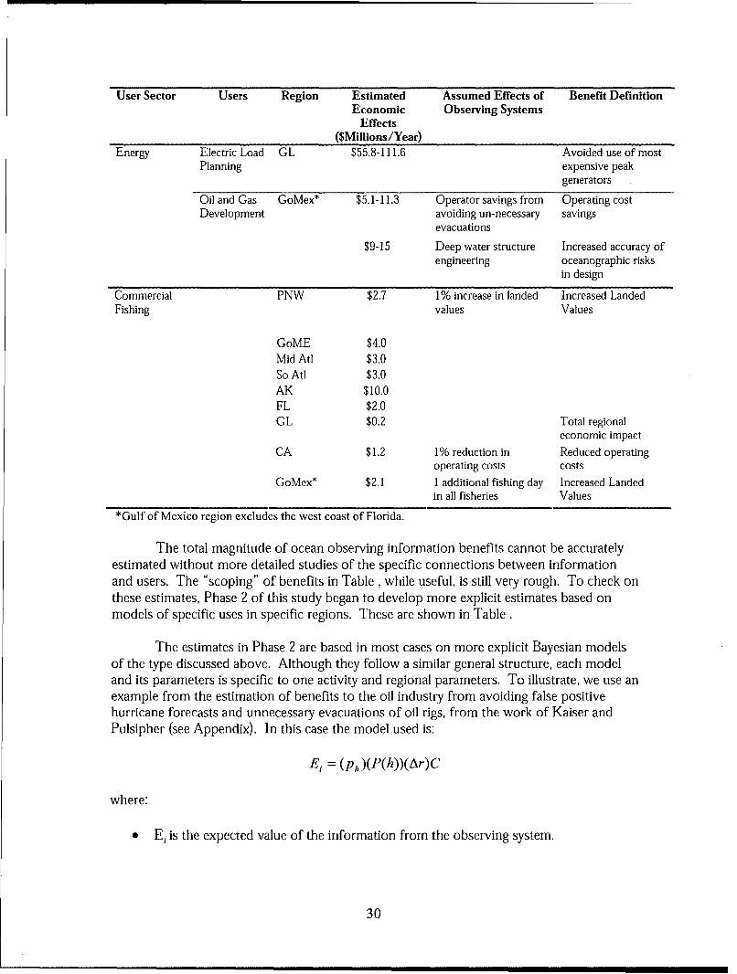
User Sector Users Region Estimated Assumed Effects of Benefit DefinitionEconomic Observing Systems
Effects($Millions/Year)
Energy Electric Load GL $55.8-111.6 Avoided use of mostPlanning expensive peak
generators
Oil and Gas GoMex* $5.1-11.3 Operator savings from Operating costDevelopment avoiding un-necessary savings
evacuations
$9-15 Deep water structure Increased accuracy ofengineering oceanographic risks
in design
Commercial PNW $2.7 1% increase in landed Increased LandedFishing values Values
GoME $4.0Mid Atd $3.0So Ati $3.0AK $10.0FL $2.0GL $0.2 Total regional
economic impactCA $1.2 1% reduction in Reduced operating
operating costs costsGoMex* $2.1 1 additional fishing day Increased Landed
in all fisheries Values
*Gulf of Mexico region excludes the west coast of Florida.
The total magnitude of ocean observing information benefits cannot be accuratelyestimated without more detailed studies of the specific connections between informationand users. The "scoping" of benefits in Table , while useful, is still very rough. To check onthese estimates, Phase 2 of this study began to develop more explicit estimates based onmodels of specific uses in specific regions. These are shown in Table.
The estimates in Phase 2 are based in most cases on more explicit Bayesian modelsof the type discussed above. Although they follow a similar general structure, each modeland its parameters is specific to one activity and regional parameters. To illustrate, we use anexample from the estimation of benefits to the oil industry from avoiding false positivehurricane forecasts and unnecessary evacuations of oil rigs, from the work of Kaiser andPulsipher (see Appendix). In this case the model used is:
Ei = (Ph)(P(h))(Ar)C
where:
* Eis the expected value of the information from the observing system.
30
" Ph describes the probability of a hurricane in the Gulf of Mexico, the path of whichcould be better predicted with ocean observing system information. In thiscalculation the frequency is assumed to be one hurricane per year.
" P(h) is the number of platforms in the Gulf (here assumed to be 750) multiplied by(h) the proportion of rigs potentially affected by the hurricane. h is assumed to be.13, for a total of 100 potentially affected rigs.
" Ar is the change in forecasting accuracy due to the observing system. In this case,there is an assumed 10-20% reduction in the probability of a false positive forecastthat a hurricane will hit a specific set of rigs.
"* C is the cost of evacuating a rig, estimated at $10,000 per platform and $50,000 perrig.
The resulting calculation is:
(750) (0.1-0.2) ($10,000-$50,000) =$1.25-2.5M
Details on the specific forms for each model and/or supporting information arediscussed in the Appendices.
The Phase 2 results in Table 10 are generally of the same order of magnitude as thePhase 1 results in Table 9, which suggests that the range of estimates is reasonable. Theavailable social surplus estimates (the correct measure of economic benefits) range from$187 million to $200 million per year. For a limited array of regions and users, these figuressuggest benefits that will likely easily exceed investment and operating costs from theobserving systems when scaled up to national levels and when the non-social surplusestimates can be appropriately disaggregated.
There are still weaknesses in the data, however, as gross values are still required forsome of the estimates, particularly in the fisheries. One exception is the study by Wellmanand Hartley on Alaskan fisheries, which develops estimates of producer surplus changesfrom more accurate forecasts of fish stock levels in the Bristol Bay salmon fishery. There,the short time of the open fishery and its remoteness from larger settlements places severerisks on companies, which must precisely estimate the amount of labor and capital they willemploy each year or risk either cost penalties from overstocking supplies and labor or severeprofit penalties from under-stocking them. This case provides a good example of possiblebenefits where the ocean observing system information could be highly useful to business-critical decision making, although even here the probability of benefits for now must rest onthe judgment of those engaged in the fishery. At the same time, this is one of the fewexamples in the fishery where cost data needed for estimates of changes in producer surplusare available.
31
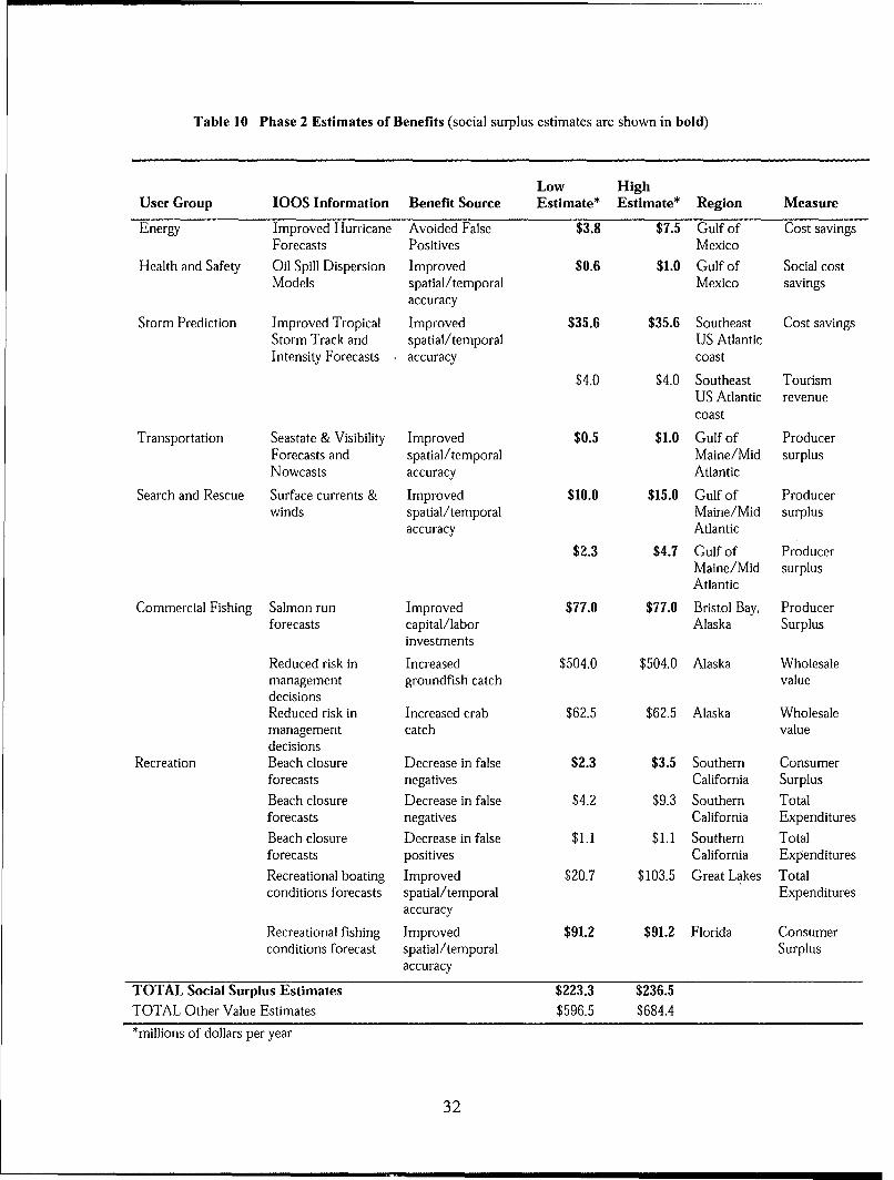
Table 10 Phase 2 Estimates of Benefits (social surplus estimates are shown in bold)
Low HighUser Group IOOS Information Benefit Source Estimate* Estimate* Region Measure
Energy Improved Hurricane Avoided False $3.8 $7.5 Gulf of Cost savingsForecasts Positives Mexico
Health and Safety Oil Spill Dispersion Improved $0.6 $1.0 Gulf of Social costModels spatial/temporal Mexico savings
accuracy
Storm Prediction Improved Tropical Improved $35.6 $35.6 Southeast Cost savingsStorm Track and spatial/temporal US AtlanticIntensity Forecasts accuracy coast
$4.0 $4.0 Southeast TourismUS Atlantic revenuecoast
Transportation Seastate & Visibility Improved $0.5 $1.0 Gulf of ProducerForecasts and spatial/temporal Maine/Mid surplusNowcasts accuracy Atlantic
Search and Rescue Surface currents & Improved $10.0 $15.0 Gulf of Producerwinds spatial/temporal Maine/Mid surplus
accuracy Atlantic
$2.3 $4.7 Gulf of ProducerMaine/Mid surplusAtlantic
Commercial Fishing Salmon run Improved $77.0 $77.0 Bristol Bay, Producerforecasts capital/labor Alaska Surplus
investments
Reduced risk in Increased $504.0 $504.0 Alaska Wholesalemanagement groundfish catch valuedecisionsReduced risk in Increased crab $62.5 $62.5 Alaska Wholesalemanagement catch valuedecisions
Recreation Beach closure Decrease in false $2.3 $3.5 Southern Consumerforecasts negatives California Surplus
Beach closure Decrease in false $4.2 $9.3 Southern Totalforecasts negatives California Expenditures
Beach closure Decrease in false $1.1 $1.1 Southern Totalforecasts positives California Expenditures
Recreational boating Improved $20.7 $103.5 Great Lakes Totalconditions forecasts spatial/temporal Expenditures
accuracy
Recreational fishing Improved $91.2 $91.2 Florida Consumerconditions forecast spatial/temporal Surplus
accuracy
TOTAL Social Surplus Estimates $223.3 $236.5
TOTAL Other Value Estimates $596.5 $684.4*millions of dollars per year
32
Estimates of consumer surplus also have potential weaknesses. There are dozens ofstudies of the economic value of beach recreation, but there is also large variation in theresults of what a beach day is worth. Estimates cited in studies used here range from about$7.00 per day to $28.00 per day. The variances in values arise from a number of sources,most importantly the sampling and estimating methodologies used. Some studies use aversion of contingent valuation, a method based on surveys of beach users. Others used thetravel cost method, in which the costs of travel to beaches are used as a proxy for willingnessto pay.
Whatever methods are used, there are difficult issues of substitution, particularlyamong recreation users. To return to the surfer example: when a beach is closed or is openwith unfavorable conditions, the surfer may simply choose another beach. Some benefitsfrom the observing system may be realized if its information is used to make this selection,and so it is unclear whether the benefits are increased from the ability to substitute, orreduced somewhat because the substitute requires higher travel costs (and thus lowerpotential net benefits). A similar problem of substitution arises for recreational boating andfishing activities.
As a result of these data issues, the estimates presented here are best used to suggestan order of magnitude for potential benefits of ocean observing systems. These are shownin Table 11. The data in this table are for estimated annual potential benefits. For thosedesignated as "l0s" of thousands, benefits likely range from $10,000 to $90,000 per year,while those designated in the "100s" benefits likely range from $100,000 to $900,000 peryear.
Table II Order of Magnitude Estimates of Benefits by Major Users
Order of magnitude of Regions withpossible annual benefits greatest benefits(millions of dollars)
Recreational Activities Recreational Fishing 100s Great Lakes, Gulfof Mexico
Recreational Boating 100s Great Lakes, Gulfof Mexico, Atlantic
Beaches/Shore Recreation loos Florida, CaliforniaTransportation Transportation-Freight los Florida, Mid
AtlanticTransportation-Cruise Ships los Florida
Health and Safety SAR los AllOil Spills los AllTropical Storm Prediction los Atlantic, Gulf of
MexicoEnergy Electricity Load Planning 1os to 100s Great Lakes,
California, AtlanticOcean Structures los Gulf of Mexico
Commercial Fishing Commercial Fishing loos Alaska, NewEngland
33

34
Conclusions and Recommendations
The data in Table 11 suggest that annual benefits to users in the United States fromthe deployment of coastal ocean observing systems are likely to run in the multiple $100s ofmillions of dollars per year. On a discounted present value basis over time, the benefitsfrom a national investment in such systems are likely to exceed the costs (though theseremain to be quantified carefully). This finding is consistent with previous conclusions onthe economic benefits of such systems, such as that of Kite-Powell and Colgan (2001)10 onthe Gulf of Maine.
The data also indicate that ocean observing systems will have the largest benefitswhere the information from such systems is used by the largest possible groups. Benefitsfrom recreational activities consistently generate the greatest values because of the very largenumber of people who use beaches, boat on the Great Lakes or in the coastal ocean, orengage in marine recreational fishing. Although the per-user benefits are smaller than thoserealized in other user sectors, the large number of users drives the overall magnitude ofpotential benefits to substantial sums.
Several important caveats are required in interpreting the results of this study:
" The fact that the benefits from the systems as a whole will exceed the costs does notmean that the benefits will exceed the costs in every individual case. Theconfiguration of observing systems in each region should take into account thepriorities of user local and regional user groups.
The estimates presented assume:
"* Full and successful deployment of existing, near-deployment, or reasonablyforseeable technologies.
"* Cost efficient and effective means of communicating the information derived fromthe ocean observations to users in a timely manner.
"* Users are aware of, and effectively incorporate, the information into their decisionsregarding their activities.
" In the case of commercial fisheries, additional information concerning the state ofthe marine environment is relevant to decisions about managed fisheries and (atsome point) will permit increases in allowable catches.
Violation of any of these assumptions may reduce the potential or actual benefits to levelsbelow those estimated here.
10 Kite-Powell, H.L. and C.S. Colgan 2001 The Potential Economic Benefits of Coastal Ocean ObservingSystems: The Gulf of Maine. Marine Policy Center Woods Hole Oceanographic Institution.
35
Based on these findings, we believe additional research is needed to develop moreprecise estimates of benefits for specific observing systems, instruments, technologies, andapplications. Specifically:
* Operators of regional observing systems should incorporate in their operationalplans strategies and activities to measure the economic benefits of their products andservices.
Each of the regional observing organizations is expected to undertake some form ofregular estimates of benefits." This will require two pieces of information: the number ofusers and the value placed on the use. Regular evaluation of regional observing systeminformation will require close monitoring of the number of users of different informationproducts, and should include verification not only of the number of users but how theyutilize the information.
Valuation of information uses can be accomplished in several ways. For example,user surveys incorporated into websites that distribute observing system information couldbe an effective tool to measure both the number of users and the values they put on theinformation. As was done in this study, benefit studies performed for other purposes maybe used to infer values associated with observing system information, although carefulreview of such studies is required to assure both theoretical and empirical appropriateness.
Investments should be made by federal, state and local governments in moreprecisely estimating economic benefits and in sharing data and methods for benefitsestimation among operators of observing systems. To build on the work presentedin this report, a series of coordinated pilot projects should be funded at the regionallevel to develop, apply, and share with other regions detailed guidelines for benefittracking and estimation. These pilot projects should focus on one or two prominentuser sectors in each region, and cover the major sectors identified in this report.
Those who operate regional observing systems are likely to be experts in the oceansciences, technologies, and data management, and are unlikely to have substantial expertisein economic benefit evaluation. If the expectation of consistent economic benefitsassessment is to be met, regional associations will need access to resources, includingpersonnel, easily implementable methods, standard instruments for surveys, etc. Developingsuch methodologies on a pilot basis with different regional associations and with theintention that methods, data, etc. thus developed could be transferred nationally to themaximum extent possible, could save a great deal of potential wheel reinvention and greatlyimprove the quality and quantity of economic benefits data available for future evaluations.
* Consumer surplus benefits should be estimated for all categories of recreationalusers in various regions of the country. Current estimates of such benefits do not
See "Guidance for the Establishment of Regional Associations and the National Federation of RegionalAssociations", produced by Ocean.US (www.ocean.us. [The business plan] should describe expected benefitsfor users and how products and services will be evaluated periodically (e.g., annually) in terms of the timelyprovision of data, data quality, user satisfaction, system integration, and the achievement of the RA's objectives.
36
fully account for the possibility of substitution among different recreation resourcesin different regions and remain subject to considerable methodological variability.
The estimation of consumer and producer surplus presents two different challenges.In general, any estimates of cost savings by public or private organizations that result fromobserving information can be counted as producer surplus. The case of the Bristol Baysalmon is a good example. While cost data are far from universally available, they are moreavailable than data on consumer surplus, which is the key to measuring benefits in therecreation area. As noted above, these are likely to be the largest generators of total benefitssimply because of the number of users.
Because of the variance in consumer surplus methodologies and results, operators ofobserving systems will need both guidance on the estimation of such benefits and access toexisting and new studies. A library of accessible and relevant consumer benefits studies isone way to meet needs. There is also substantial variability in the availability of such studies.Marine recreational fishing tends to be the most intensively studied recreational activityrelevant to ocean observing systems in most of the country. Beaches are the next mostcommon, although there is great variability across regions. California and Florida tend tohave the most studies, New England the least. Recreational boating value studies are sparsein all regions. Examples of relevant resources include:
0 National Survey on Recreation and the Environment (NSRE):http://marineeconomics.noaa.gov/NSRE/
0 National Ocean Economics Project (NOEP) Non-Market Value Portal:http://noepdata.csumb.edu/nonmarket/NMmain.html
37
Contributors
Hauke L. Kite-Powell PhDMail Stop 41, WHOIWoods Hole, MA 02543-1138Phone: (508) 289-2938 FAX: (508) 457-2184 E-mail: hauke(@iwhoi.edu
Charles S. Colgan PhDMuskie School of Public ServiceUniversity of Southern MainePO Box 9300 Portland, Maine 04104Phone: (207) 780-4008 FAX: (207) 780-4417 E-mail: csc(ausm.maine.edu
Michael Luger PhDUNC Chapel Hill, Campus Box 3440, The Kenan CenterChapel Hill, NC 27599-3440Phone: (919) 962-8201 FAX: (919) 962-8202 E-mail: mluger(aemail.unc.edu
Ken Wieand PhDCollege of Business Administration, University of South FloridaTampa, FL 33620Phone: (813) 974-3629 FAX: (813) 905-5856 E-mail: kwieand(icoba.usf.edu
Allan G. Pulsipher PhD Mark J. Kaiser PhDCenter for Energy Studies, Louisiana State UniversityBaton Rouge, LA 80893Phone: (225) 578-4550 FAX:(225) 578-4541 E-mail: agpul(alIsu.edu
Linwood Pendleton PhDSchool of Public HealthUniversity of California at Los AngelesLos Angeles, CAPhone: (805) 794-8206 E-mail: [email protected]
Katharine F. Wellman PhD261142 d Ave. W.Seattle, WA 98199Phone: (206) 284-2413 E-mail: kfwellman(&,attbi.com
Thomas M. Pelsoci PhDDelta Research Co.Two First National Plaza, 20 S. Clark Street, Suite 620, Chicago, IL 60603Phone: (312) 332-5739 FAX: (312) 372-3874 E-mail:tpelsoci(odeltaresearchco.com
38
Acknowledgements
We thank the member agencies of the National Oceanographic Partnership Program fortheir support in the funding of this study. Agencies contributing to the study included theNational Oceanic and Atmospheric Administration, Office of Naval Research, NationalScience Foundation, National Aeronautics and Space Administration, United States CoastGuard, Environmental Protection Agency, and Minerals Management Service.
Dr. Rodney Weiher of NOAA served as Project Administrator for NOPP. Dr. MelbourneBriscoe of the Office of Naval Research served as Project Coordinator.
Our appreciation also goes to the staff of Dr. Tom Malone, Dr. Larry Atkinson, Muriel Cole,and the staff of Ocean.US who provided valuable technical assistance and facilities for theproject team to meet. We also thank Margaret Davidson of the NOAA Coastal ServicesCenter for providing additional funding support.
The Global Ocean Observing System Steering Committee, and its chair, Dr. Worth Nowlinof Texas A&M University provided input and assistance through the project.
39

40
Appendix A: Beach Management in California
Linwood PendletonUniversity of California, Los Angeles
41
Harnessing Ocean Observing Technologies to Improve Beach Management:Examining the Potential Economic Benefits of an Improvement in the Southern
California Coastal Ocean Observing System
July 19, 2004
Linwood PendletonAssociate Professor
Environmental Science and Engineering ProgramSchool of Public Health
University of California, Los Angeles
Acknowledgments
Special thanks are owed to: Steve Weisberg for his help in identifying ways in whichimproved coastal ocean observing technologies could be applied to coastal water qualitymanagement, Stan Grant and Eric Terrill for explanations of the way in which animproved COOS could improve a geographic understanding of the fate and dispersion ofhuman pathogens in the coastal zone, Jessica Morton for research assistance, andAlexandria Boehm, Sharyl Rabinovici, and Michael Hanemann for their commentsduring a presentation of the paper at Stanford University.
42
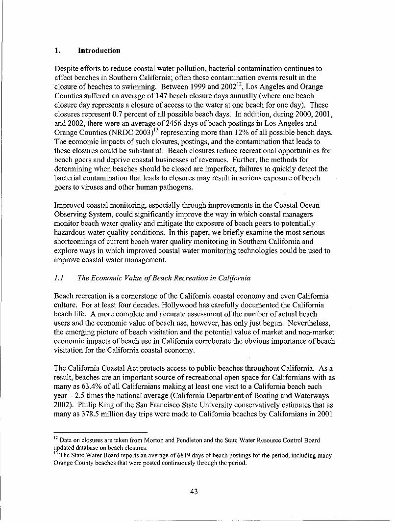
1. Introduction
Despite efforts to reduce coastal water pollution, bacterial contamination continues toaffect beaches in Southern California; often these contamination events result in theclosure of beaches to swimming. Between 1999 and 200212, Los Angeles and OrangeCounties suffered an average of 147 beach closure days annually (where one beachclosure day represents a closure of access to the water at one beach for one day). Theseclosures represent 0.7 percent of all possible beach days. In addition, during 2000, 2001,and 2002, there were an average of 2456 days of beach postings in Los Angeles andOrange Counties (NRDC 2003)13 representing more than 12% of all possible beach days.The economic impacts of such closures, postings, and the contamination that leads tothese closures could be substantial. Beach closures reduce recreational opportunities forbeach goers and deprive coastal businesses of revenues. Further, the methods fordetermining when beaches should be closed are imperfect; failures to quickly detect thebacterial contamination that leads to closures may result in serious exposure of beachgoers to viruses and other human pathogens.
Improved coastal monitoring, especially through improvements in the Coastal OceanObserving System, could significantly improve the way in which coastal managersmonitor beach water quality and mitigate the exposure of beach goers to potentiallyhazardous water quality conditions. In this paper, we briefly examine the most seriousshortcomings of current beach water quality monitoring in Southern California andexplore ways in which improved coastal water monitoring technologies could be used toimprove coastal water management.
1.1 The Economic Value of Beach Recreation in California
Beach recreation is a cornerstone of the California coastal economy and even Californiaculture. For at least four decades, Hollywood has carefully documented the Californiabeach life. A more complete and accurate assessment of the number of actual beachusers and the economic value of beach use, however, has only just begun. Nevertheless,the emerging picture of beach visitation and the potential value of market and non-marketeconomic impacts of beach use in California corroborate the obvious importance of beachvisitation for the California coastal economy.
The California Coastal Act protects access to public beaches throughout California. As aresult, beaches are an important source of recreational open space for Californians with asmany as 63.4% of all Californians making at least one visit to a California beach eachyear - 2.5 times the national average (California Department of Boating and Waterways2002). Philip King of the San Francisco State University conservatively estimates that asmany as 378.5 million day trips were made to California beaches by Californians in 2001
12 Data on closures are taken from Morton and Pendleton and the State Water Resource Control Board
urdated database on beach closures.1- The State Water Board reports an average of 6819 days of beach postings for the period, including manyOrange County beaches that were posted continuously through the period.
43
(California Department of Boating and Waterways, Chapter 3). The United States LifeSaving Association estimates that as many as 146 million visitor days were made tosouthern California beaches alone (USLA 2002). In another study Morton and Pendleton(2001) estimate that total beach attendance in Los Angeles and Orange County in 2000exceeded 79 million visits. Morton and Pendleton's estimates, detailed in a report to theState Water Resources Control Board, are taken directly from lifeguard records.
Day trips to beaches generate two distinct sources of economic value for the coastal andocean economy: market expenditures and non-market consumer surplus values. First,day visitors to beaches spend money locally on food, beverages, parking, and beachrelated activities and rentals (e.g. body boards, umbrellas, etc.). These expenditurespartially represent a transfer of expenditures that may have been made elsewhere in thestate (e.g. gas and auto), but are largely expenditures that would not have been made inthe absence of the beach trip. We use two previous studies to estimate the averageexpenditures per person per day trip ($/trip/person) for visits to California beaches. Asurvey of beach goers in southern California (Hanemann et al. 2002) found that perperson per trip expenditures on beach related items and services were $23.19 for beachgoers that took at least one trip in the summer of 2000. In another study by King(California Department of Boating and Waterways 2002), average beach relatedexpenditures (excluding gas and automobile costs) were $29.66. Based on these twostudies, we conservatively estimate the average per trip per person beach relatedexpenditure for California beach visits to be $25 and the total annual beach relatedexpenditures to be $9.46 billion. We estimate the total annual expenditures for beachgoers in Los Angeles and Orange Counties to be $1.8 billion.
Visitors to beaches also place a value on beach visits above and beyond what they spendat the beach - the consumer surplus of beach visits. Unlike many marketed goods, accessto the beach is largely free (aside from parking fees) in California. Because of the lowcost of beach access and the importance of beach recreation to Californians, numerousstudies have estimated the consumer surplus of beach going in California to bettermeasure the true value of beaches and beach management in the state. Two primarymethods were used to value consumer surplus estimates: the travel cost method and thecontingent valuation method. Chapman and Hanemann (2001) argue that to datecontingent valuation estimates of California beach visits have been flawed and generateunreliable estimates of beach values, largely because the contingent valuation surveysoften are not site specific and fail to account for varying travel costs to beaches aroundthe state.
Travel cost estimates of consumer surplus for beach visits have been employed toestimate the value of visits to beaches, largely along the central and southern Californiacoast. Table 1 provides estimates of consumer surplus values for visits to beaches inCalifornia. Consumer surplus estimates range from a low of $10.98 (in 2001 dollars) forvisits to Cabrillo Beach in Los Angeles County (Leeworthy and Wiley 1993) to a high ofgreater than $70 (in 2001 dollars) per person per trip for visits to San Diego beaches(Lew 2002). In 1997, Michael Hanemann estimated the value of the consumer surplus ofbeach visits to Huntington Beach at $15/visit (Hanemann 1997). Hanemann's estimate of
44
beach related consumer surplus was later discounted by ten percent and used as the basisfor a jury award regarding lost beach recreation due to the American Trader oil spill(Chapman and Hanemann 2001). More recent results, still under review, by the SouthernCalifornia Beach Valuation project indicate that in Southern California alone, the non-market value of swimming at beaches may exceed $1 billion 14 and the value of visits tobeaches for swimming and non-swimming activities may exceed $2 billion.
1.2 Current Procedures for Determining Beach Closures
An improved and substantially modified in the Coastal Ocean Observing System couldimprove the accuracy of the system used to determine when and where beaches areclosed in Southern California. The state of California, through State Bill AB 411,mandates the closure of beaches that are thought to be contaminated by sewage andrequires the "posting" of beaches that exceed specific levels of bacteriologicalconcentrations. Currently, the procedures used to close beaches to swimming rely on anotification of sewage spills by sanitation authorities or in situ measures ofbacteriological water quality. Only rarely are sewage spills detected immediately andsometimes even known spills are not reported to the public.15 Heal the Bay reports thatbetween April 2002 and March 2003 there were 222 sewage spills in Los Angelescounty, none of which led to beach closures (including one spill that emitted 745 gallonsof untreated sewage into the waters of Will Rogers State Beach)16 . More commonly,water quality impairment is discovered by the daily water sampling that is conducted atstations along California's beaches; sewage spills are often reported by beach goers andresidents. These samples are collected in the surf zone and sent to labs for analysis.
Three serious shortcomings exist in the methods used to monitor water quality andinform the public about water quality contamination. First, weekly and even daily watersampling is known to be an extremely imprecise means of detecting water qualitycontamination by bacteria (see for instance Leecaster and Wiesberg 2001 or Kim andGrant 2004.) The effects of tides, lunar cycles, and other vagaries in near shoreoceanographic conditions can seriously impair the effectiveness of surf zone and "pointzero" storm drain monitoring. Temporarily high bacteria readings may not indicatecontinued serious coastal water contamination while at other times a false negativereading may mask serious contamination problems. Leecaster and Weisberg (2001)found that only thirty percent of positive first day readings were associated withsignificant water quality contamination during the following day. The findings ofLeecaster and Weisberg indicate that by the time water quality contamination is detected,water quality has returned to normal in seventy percent of the cases. Kim and Grant(2004) estimate that at Huntington State Beach, current water quality methods result inerrors of public posting that can reach forty percent at times.
14 The estimates of Hanemann et al are not weighted to reflect sampling bias and so should be considered as
an order of magnitude estimate for non-market swimming values.15 For instance, on March 3, 2004 the Hyperion Treatment plant released more than 150,000 gallons ofpartially treated effluent into Santa Monica Bay, but the release was not reported publicly until March 5,2004.16 See www.healthebay.org
45
A second serious problem with current water quality monitoring efforts is that asignificant time lag exists between water sample collection and the reporting oflaboratory results; the time between sampling and the determination of water quality cantake up to three days. This lag suggests that potentially harmful water quality conditionsmay exist for as long as three days before the public is notified. (The time lag is evenlonger for beaches that have only weekly sampling.) Further, water quality conditionsmay have improved substantially by the time that results are reported. The practicalresult of these time lags is that many beaches remain open when they should be closedand are closed after they should have been re-opened. The economic impact of thisdissonance between monitoring and closures is that a) beach goers may get sick fromswimming at beaches where water quality has been shown to be impaired and b)recreational beach goers may be prevented from visiting beaches that are no longercontaminated and therefore need not be closed.
Finally, the indicator bacteria currently monitored by water quality agencies provides aninexact determination of the source of water quality contamination. Indicator bacteria arenot specific to human beings and may result from natural sources. The reliance on theseindicator bacteria as proxies results in two types of monitoring errors. First, positiveindications of water quality contamination may be inappropriately linked to humansources. This may have been the case at Huntington Beach during the closures of 1999.Second, without primary data indicating the presence of human pathogens, somecontaminated beaches may remain open because the actual link between human sewageand bacteria levels remains undetected. Without knowledge of an active sewage spill orother source of contamination by human wastes, beaches may only be posted and notclosed; the result is that bathers may continue to use posted waters believing that thecontamination risk is less serious than during a closure".
Once a high level of bacteria has been detected, managers must determine the extent ofbeaches that may be impacted. If a sewage spill is known to be associated with highlevels of water borne bacteria, managers often close large sections of beach. If two ormore sampling stations indicate high-levels of potentially sewage-related bacteria, thenbeach areas adjacent to and between stations will be closed. Such extensive closures areintended to provide closures that err on the side of precaution. Nevertheless it is knownthat bacteria from point sources (e.g. stormdrains or breaks in sewer lines) are notdispersed uniformly throughout the surf zone. Instead, bacteria and pathogens followlocal near shore currents. The results are hotspots of bacterial contamination that mayaffect only very small sections of the shoreline. Steve Weisberg, Director of the SouthernCalifornia Coastal Water Research Project, estimates that the geographical imprecision ofcurrent beach closure protocols may result in the closure of as much as two times moreshoreline than is needed to protect beach goers from coastal bacterial water pollution.The economic result of this imprecision is that beach goers are unnecessarily displacedfrom beaches; non-market values and expenditures are diminished unnecessarily.
17 There are no empirical data that indicate the effect of postings on swimmer behavior.
46
For the purposes of analysis, we group the policy errors associated with the shortcomingsof the current protocol for monitoring and reporting water quality data into two types oferrors in the execution of beach closure policy (we follow the example of Rabinovici etal. 2004). First, in some the current protocol causes beaches to be closed when thesebeaches are, in fact, in compliance with water quality standards; we refer to these types oferrors as Type I errors and note that these errors largely impact the recreational value ofbeaches. Second, time lags in reporting and a failure to adequately identify humanpathogens in coastal water quality leads to a Type II error in which beaches are not incompliance with water quality standards for safe swimming, but beaches are not closed toswimming (in many cases these beaches may be posted with advisories). Type II errorsresult primarily in public health costs. Of course, it is unlikely that Type I and II errorscould ever be eliminated completely. Nevertheless, in the discussion that follows webegin to estimate an upper bound for the value of the elimination of these errors in themanagement of beaches in Los Angeles and Orange Counties.
1.3 Using the SCCOOS To Better Manage Beach Postings and Closures
We use a basic framework of "models" to explore and evaluate the potential policyimpacts of improvements in the SCCOOS that could improve the monitoring of coastalwater quality. The first model in the framework begins with a description of theproposed technologies and the resulting data and analyses that would be part of theimproved SCCOOS. We call this model "NOWCASTS AND FORECASTS." New rawdata and analyses will become part of the portfolio of information that coastal managersuse to make decisions regarding coastal water quality and beach closures. In theDECISION MODEL we describe these basic decisions and how they are affected by theinformation that could be generated by improvements in the SCCOOS. The decisionsmade by coastal managers in turn result in real changes in the behavior, health, and wellbeing of beach goers. In the PHYSICAL MODEL, we describe the policy and behavioraloutcomes of that result from better decision making. Finally, in the ECONOMICMODEL we begin to put the physical outcomes in the context of potential economicchanges that might result from this potential, but hypothetical, use of improved coastalocean observing technology.
2. NOWCAST AND FORECASTS
The Southern California Coastal Ocean Observing System could be modified to betterdetect, track, and monitor coastal ocean contamination; two primary technologies couldbe employed towards this end. First, several technologies, broadly known as RapidMicrobial Indicator Methods, now exist that permit the immediate detection andidentification, and thus reporting, of bacteriological pathogens in coastal waters (ACT2003). In June 2004, the Southern California Coastal Water Research Project began atest of three principal types of rapid microbial indicator methods: Immunoassays,Chromogenic Substrate Analyzers, and Polymerase Chain Reaction Methods. Thesemethods could improve beach water quality monitoring by a) providing continuousmonitoring of water quality (thus providing more data to help overcome the temporal
47
vagaries that affect water quality testing), b) more accurate detection of humanpathogens, and c) real time (or near real time) notification of health risks (i.e. reducedtime lag between sampling and reporting). Secondly, oceanographic buoy data (e.g.wind, waves, current, temperature) can be combined with satellite data to more accuratelymodel, and thus predict, the fate of water borne pathogens near the coast. Systems likethe CODAR (personal communication, Eric Tyrell, Scripps Institute of Oceanography),already part of the Southern California Coastal Ocean Observing System, havedemonstrated the potential for more accurately tracking the source and dispersion ofcontaminants in coastal areas of San Diego County including the Tijuana River outfall.Stanley Grant of the University of California, Irvine proposes a similar system in whichHF Radar data, NEOCO data, mooring data, and ocean current modeling efforts will belinked to existing water quality monitoring programs, to create a water quality forecastingalgorithm suitable for deployment at coastal sites (personal communication). Betterprediction of the fate of contaminants will allow managers to more narrowly targetbeaches for closure and also will allow authorities to close beaches that are likely to beaffected by contaminant flows in advance of actual detection at those beaches.
3. DECISION MODEL
The data from the potential improvements in the SCCOOS, described above, will be usedto inform three types of policy actions:
1) when pathogens levels are sufficiently high to warrant beach closures, whichbeaches should be closed,2) the provision of accurate information to the public regarding the geographicalextent and duration of water quality contamination events, and3) the determination of the existence of human pathogens in coastal waters.
By better informing these three areas of policy decision making, the improved SCCOOScould substantially reduce the kinds of errors in identification and reporting of waterquality contamination problems.
4. PHYSICAL OUTCOMES MODEL
4.1 General Outcomes
The provision of more timely and accurate data about the extent and duration of coastalwater quality contamination would result in a number of tangible policy outcomes. Wereview these outcomes here and in the next section describe and begin to place a valueupon the economic impacts of these outcomes.
4.2 Type I and Type II Errors in Closing Beaches
As described above, an improved SCCOOS could potentially improve the accuracy ofwater quality monitoring and in turn would improve the economic and public healthefficiency of the current system of beach monitoring and closures. Following Rabinoviciet al. (2004), we examine the ways in which an improved SCCOOS could reduce the twoprimary errors made by beach managers: Type I errors in which beaches are in
48
compliance with water quality standards, but are inappropriately closed to swimming andType II errors in which beaches are not in compliance with water quality standards, butare not closed to swimming.
4.2.1 Type I ErrorsSpecifically, the improved SCCOOS could potentially
"* reduce false positive pathogen indications that are caused by temporallyvarying water conditions and sampling regimes,
"* reduce false positives that are caused by non-human bacteria, and"* improve the geographic accuracy of closures by using models and real
time data collection to determine areas most likely to be contaminatedfollowing a detection.
We begin our exploration of the economic benefit of reducing Type I errors by focusingon the gains from a better geographic understanding of the fate of waterborne pathogensand assume that the economic value of such improvements would come from reducing byhalf the spatial extent, and thus the number, of unnecessary closures.
4.2.2 Type II Errors:Improvements in the SCCOOS could reduce the number of days in which beaches arecontaminated and should be closed, but are not closed. These Type II errors occur fortwo primary reasons: 1) the time lag between sampling and monitoring means that severewater quality impairment is not reported to the public until two or more days after thewater quality event and 2) some contaminated beaches are not closed if authorities cannotdetermine a link between human sewage and high levels of bacteria. Type II errorsprimarily have public health impacts; swimmers on these days are likely to get sick morefrequently than on uncontaminated days.
Turbow, et al. (2003) show that most illnesses occur even when beaches remain open, butare posted. The deployment of rapid microbial indicators methods could lead to animprovement in the accuracy of detection of human pathogens and the ability toaccurately differentiate between high levels of non-human fecal bacteria and the morevirulent human pathogens. As noted at the beginning of this report, the NRDC reportsthat, on average, more than 2450 beach postings are made Los Angeles and OrangeCounty. In fact, the State Water Board's beach posting database indicates as many as6000 postings on average over the period 1999-2002. Many of these postings are likelyto represent serious human health hazards; with better pathogen identification many ofthese posting might become closures. (Postings are likely to be an imperfect means ofeliminating swimming at contaminated beaches. Therefore, the conversion of postings toclosures when appropriate would further reduce exposure to pathogens and represent afurther decline in the number of Type II errors that are made by beach managers.)
49
5. ECONOMIC OUTCOME MODEL
5.1 Recreational Impacts
We begin by examining an upper bound for the value of reducing Type I errors thatcreate inappropriate closures and thus diminish recreational values associated with beachuse. Beach closures represent a loss of recreational opportunities for beach goers inSouthern California. Rabinovici et al (2004) show that for Great Lakes beaches, a beachclosure represents a net economic loss to society even when the beach should have beenclosed under public health guidelines. In our analysis, we focus only on the value ofbeach closures during which visitors may have been prevented from swimming on dayswhen water quality might have fallen within the range of bacteriological levels deemedsafe by public health standards. As stated above, we limit our analysis here to the value ofreducing by half the number of unnecessary beach closures in Los Angeles and SouthernCalifornia. Under this scenario, there would be an additional 73.5 beach days availableto beach goers in Southern California.
Hanemann et al. (2004) show that the exact value of a beach closure in SouthernCalifornia depends on the beach in question and the season of the closure. Predictingwhich beaches will close in the future, when, and how long those beaches might remainclosed or open more often with an improved COOS is not possible. Nevertheless, weexamine an upper bound for the potential value of reduced unnecessary beach closures byassuming that future unnecessary beach closures would be random.
On average, in Los Angeles and Orange Counties there were 147 beach days lost toclosures each year from 1999 to 2002. Based on 51 primary public beaches in LosAngeles County, these closures represent approximately 0.07% of all possible beach "daytrip" recreational possibilities. In fact, the entire beach is rarely closed to visitors; insteadisolated stretches of beach are closed and often these closures apply only to swimmers.As an upper bound, we assume that the entire beach is closed due to a beach closure, butwe limit this closure to that proportion of visitors that would swim at the beach.Pendleton et al. (2001) found that 38.4 % of beach goers in Los Angeles planned to swimduring their trip to the beach. In a more recent study, Hanemann et al. (2004) found that28% of all trips made to the beach by a panel of beach goers in four southern Californiacounties include a water based activity. In this study, we assume that 28% of all beachday trips in Southern California include a water-based activity.
We explore two methods for calculating the economic value of reduced unnecessaryclosures: 1) an estimation of the increase in total beach visitation and thus an increase inper trip non-market values and expenditures and 2) an estimation of a proportionalincrease in total non-market and expenditure values for Southern California beachvisitation.
METHOD 1: VALUING AN INCREASE IN TOTAL BEACH VISITATIONIn the first method, we use an average daily attendance figure for beaches closed in 1999and 2000 to estimate the total number of beach visits that could be recovered. Average
50
daily beach attendance, at all reporting beaches in Los Angeles and Orange Countiesduring 1999 and 2000 was 8,142 visitors/beach day. (The average daily attendance, twodays before closure, at closed beaches in 1999 was 8,606 visitors/beach day6 . Thisindicates that from an attendance perspective, the beaches that were closed in these yearswere slightly less more heavily visited than beaches on average; in other words, popularbeaches were being closed.) Based on the assumptions outlined above, approximately167,500 new beach visits could have been made were there better geographic resolutionof beach closures. As described earlier, we value a beach visit at $13.50/visit/beach dayand the per person expenditures are estimated to be $25/visit/beach day.
Method 1: Non-market valuation -(Average visits/day) x (proportion of visitors that swim) x (additional beachdays) x (value of a beach day) = recreational value of reducing unnecessaryclosures.
(8142 visits/beach day) x 28% (swimmers/total visitors) x 73.5 beach days x$13.50/visit = $2,262,000
Method 1: Market Valuation(8142 visits/beach day) x 28% x 73.5 beach days x $25/visit/beach day=$4,189,000
METHOD 2: VALUING A PROPORTIONAL INCREASE IN TOTAL VALUESAs a check on our estimates from Method 1, we consider the change in value that wouldhave resulted had there been a proportional increase in the total non-market value andtotal expenditures associated with beach visits in Los Angeles and Orange Counties. Inreality, a proportional increase assumes that the provision of more beach recreationalopportunities would lead to a linear increase in value. Such a proportional increaseshould be considered an upper bound on the potential impact of additional beach days.First, a proportional increase assumes that the non-market value of additional beach daysis equal to the average value of all other beach days. In fact, the value of these additionalbeach days depends on whether or not these additional beach days represent better thanaverage or worse than average beach recreational opportunities. Second, it may be thecase that a proportional increase in beach opportunities will not lead to a proportionalincrease in beach visits of the same size. Therefore, our estimates of the value of aproportional change in beach expenditures also should be considered an upper bound.
Method 2: Non-market ValuationCurrent total non-market value of water related activities x (additional beachdays/ total beach days) = change in non-market value
$1 billion18 x (0.0035) = $3,500,000
18 The estimates of Hanemann et al are not weighted to reflect sampling bias and so should be considered
an order of magnitude estimate for non-market swimming values.
51
Method 2: Market ValuationCurrent total expenditures x (swimmers/total visitors) x (additional beach days/total beach days) = change in market value$9.46 billion x .28 x .0035 =$9,270,000
Using the more conservative estimates from the two methods, we find that bettergeographic accuracy in closures could yield potential economic benefits of: $2,262,000for non-market values and $4,189,00 for expenditures for a total of $6, 451,000/year.
(We remind the reader that the above analysis focuses exclusively on beach closures. Todate, the impact of beach postings on beach visitation has not been quantified. If beachpostings effectively eliminated beach visitation by swimmers, then our approach herecould be applied to beach postings as well. The NRDC reports an average annual numberof beach posting days in Los Angeles and Orange County of 2456. This representssixteen times more days than in the closure analysis above.)
5.2 Public Health Impacts
In the short run, public health benefits of an improved SCCOOS could come from thereduction in the time lag between sampling and reporting water quality impairments thatwould be possible with the deployment of telemetric rapid microbial indicators (i.e.microbial indicators that could transmit data in real time or near real time). Reducing thistime lag, in turn, could reduce the number of days in which beaches are contaminated, butnot closed (Type II errors in compliance). Further public health benefits would resultfrom the deployment of rapid microbial indicators that could differentiate between humanpathogens and non-human pathogens. This more precise species identification ofpathogens could potentially reduce closures that are mistakenly linked to sewage spills,but also could increase the overall number of closures by leading authorities to closebeaches that might otherwise have been posted. (These increased closures would result ina loss of recreational values. Rabinovici et al., 2004, argue that even appropriate closuresresult in recreational value losses that may exceed gains in public health values.) Wefocus only on the gains in public health values that could result from a reduction in TypeII compliance errors.
5.2.1 Cost of water related illnessesRecreational contact with marine bathing water has been shown to result in an increasedlikelihood of a suite of human illnesses including upper respiratory infections,gastrointestinal infection, ear and eye ailments, and fever. Priiss (1998) reviews theliterature prior to 1998, while a number of more recent studies further explore and modelthese links (including Henrickson et al. 2001, Wymer and Dufour 2002). Even in theabsence of known contamination by human sewage, coastal swimmers can be subject toelevated risk levels for disease (see Cabelli et al. 1982, Calderon et al. 1991, and Haile etal. 1999). Pathogens in bathing water can come from marshes (see Grant et al. 2004) andsurface water run-off (see for instance Haile et al. 1999 and Jiang et al 2001). Knowncontamination of coastal waters by human sewage has been shown to increase the relativerates of illness even more (see Fleisher 1996 and 1998). The literature does not indicate
52
whether the rates of illness are additive or whether these symptoms appear in clusters(with swimmers getting one or more illness simultaneously).
In this study, we focus exclusively on the public health impacts of bathing waters thatshould be closed to swimming due to contamination by human sewage (the principlecriterion for beach closures in Los Angeles and Orange County). Specifically, weexamine illnesses that may have resulted from a lag between sampling and the closure toswimming of beaches in Los Angeles and Orange Counties. To begin, we consider onlyexcess illnesses that may have resulted exposure to sewage contamination. In Table 2,we provide adjusted relative risk rates for the most common categories of illnessassociated with swimming in coastal waters contaminated by sewage. Column 1 givesthe proportion of swimmers that came down with illnesses after swimming in sewagecontaminated waters in the United Kingdom (Fleisher et al. 1998). For our purposes, theappropriate risk measure is that for the additional risk that comes from swimming inmarine water contaminated by sewage compared to swimming in marine water generally.Haile et al. (1999) provide estimates for the risk of illness associated with swimming inthe marine waters of Santa Monica Bay, California having very low concentrations offecal bacteria. Column 3 gives the excess risk of swimming in sewage contaminatedwaters (based on Fleisher et al.) compared to non-contaminated waters (based on Haile etal.). Of course, it is likely that the populations considered in the studies by Fleisher et al.and Haile et al. have different background levels of illness, even for non-swimmers. Infact, the rates of illness for swimmers in "clean" areas of Santa Monica Bay is generallyequal to or lower than the background levels for non-swimmers in the study by Fleisheret al. Because the background levels of sickness differ between the two studies, we useassume the net excess risk associated with swimming vs. non-swimming in the sewagecontaminated waters as a more conservative estimate of the potential excess illness thatcould result from swimming in sewage contaminated marine waters in SouthernCalifornia.
Gastrointestinal illness and ear ailments are the most common illness associated withrecreational water contact when sewage contamination is present with excess rates ofillness of 8.4 and 4.6 illnesses per 100 swimmers, respectively. Eye ailments are alsocommon more common when sewage is present, but at lower rates (2.5).
The economic impact of swimming related illnesses has not been estimated directly.Rabinovici et al (2004) use the estimated willingness to pay of $280 (in real termsadjusted to year 2000 dollars) to avoid a mild case of food-related gastrointestinal illness(estimated originally by Mauskopf and French 1991.) Bloomquist et al. (2001) valueillnesses associated with coastal bathing water by using the estimated costs of a case ofinfluenza, $380 (including the willingness to pay for illness avoidance, cost of treatment,and lost wages) originally estimated by Nichol (2001). Because gastroenteritis is 2.5times more likely in beach goers than flu-like symptoms, we follow Rabinovici et al anduse a figure of $280 for each case of excess illness.
We estimate the cost of Type II errors in compliance by assuming that bathers areexposed to contaminated water for up to two days before beaches are closed. The
53
assumption of a two day exposure is conservative; in many cases the time delay is threedays and sometimes as long as a week. Leecaster and Weisberg (2003) and Kim andGrant (2004) show that indications of water quality impairments on one day do notnecessarily result in impairments on following days. Given the unknown duration ofwater contamination during the two-day period between sampling and reporting, weassume that bathers would be exposed to contaminated water: a) for only the initial dayof sampling when a beach closure lasts for one day and b) for the two days preceding aclosure when a beach closure lasts for two days or more. To estimate the number ofbathers exposed, we combine beach attendance data and beach closure data for 1999, theonly year for which both sets of data are available' 9 . As before, we assume that 28% ofbeach goers went swimming and that water quality along the entire beach was impaired.We also assume that the swimmer may have gone swimming elsewhere had the beach inquestion been closed and thus are exposed only to the additional risk associated withswimming in sewage contaminated marine water as compared to background levels ofrisk from swimming in the same water. Following these assumptions, we find the cost ofType II errors that could be corrected by an improved SCCOOS at just over $1.25million, using the following formula:
( E Visitsi t-1 +Visitsi ,t-2 + I Visitsi,1 -2 ) x (proportion of swimmers) xi, closed >1 day j, closed I day
(adjusted excess risk x cost of illness) = cost of excess illness
(313,760 Visits) x .28 x (5.1/100) x $280 = $1,254,538
While the previous analysis focuses entirely on the public health benefits of reducingType II errors associated with beach closures, identical technology and analysis could beapplied to beach postings. Turbow et al. (2003) show that most illnesses occur whenbeaches are not closed. Bacteria levels during postings are comparable to those duringclosures and potentially could lead to substantial exposure to gastrointestinal illness of asimilar magnitude (see Cabelli et al 1982). As stated earlier, there are approximately 16times more beach posting days than beach closure days in Los Angeles and OrangeCounties. As a result, if the analysis were to be extended to beach postings and closures,the public health value would rise substantially (provided that beach postings lead tosubstantial declines in swimming at posted beaches).
6. Conclusion
The current protocol and method of monitoring recreational water quality in the UnitedStates is known to be imperfect. On site sampling, off site laboratory analysis, and areliance on fecal indicator bacteria instead of human pathogens result in two principletypes of errors associated with water quality monitoring (Rabinovici et al 2004): 1) TypeI errors in which beaches are closed even though water quality parameters are within a
19 For 9 closure days, we did not have attendance data. In these cases we used figures from the prior year
or a nearby beach.
54
"compliance" range thought to be safe for swimming and 2) Type II errors in whichwater quality parameters exceed safe "compliance" levels yet beaches are not closed.The causes of these errors include a) precautionary beach closures when a source ofcontaminants are known, but the exact fate of contaminants in near shore waters is notknown and b) lag times of two or more days between sampling and notification of waterquality impairment. Type I errors lead to a loss of recreational value when beachgoersare prevented from swimming at safe beaches. Type II errors result in public health costswhen swimmers are not adequately warned about water quality contamination.
Water quality engineers in Southern California are now testing a number of technologies,including the use of rapid microbial indicator methods and oceanographic methods, thatcould potentially reduce the incidence of Type I and II errors in beach closure policy inSouthern California. These new technologies would require modifications of the currentCalifornia Ocean Observation System including the deployment of rapid microbialindicator devices on nearshore buoys and better integration and analysis of oceanographicdata from buoys and satellites.
This study conservatively estimates the potential benefits of improving water qualitymonitoring methods in Southern California. A complete elimination of the most basictypes of errors in water quality monitoring Los Angeles and Orange County could resultin an annual economic savings of between $7.7million and $14.Omillion. These savingsare conservative because they only consider the value of public health impacts and thenon-market values of current beach users. In addition to current beach users, manyresidents and tourists are likely to avoid swimming at Southern California beachesbecause of concerns about water pollution (Pendleton 2001). Better water qualitymonitoring could have significant impacts on the public's perception of beach waterquality. Better monitoring could improve the public's confidence that beaches that areopen for swimming are, in fact, safe. This, in turn, could increase the number of peoplevisiting Southern California beaches. The potential value of these changes in perceptionshas, to date, remained undocumented, but could significantly add to the overall value ofimprovements in water quality monitoring.
Finally, in Southern California, beach closures are limited to those days in which fecalindicator bacteria levels exceed safe standards and the source of bacteria is believed to beassociated with human sewage. Beach closures represent less than six percent of the totalnumber of incidences during which water quality contamination exceeds recommended"safe" levels for swimming, but beaches are only "posted" with warning signs. Theimprovements in the coastal ocean observing system described here could be extended tothe monitoring and posting of beaches, even in the absence of sewage contamination. Abetter understanding of the impacts of these "postings" on public health and recreationalvalues is required before we can estimate the potential impacts of a reduction in Type Iand II errors in the context of beach postings.
55
7. Literature Cited
Alliance for Coastal Technologies. 2003. Rapid Microbial Indicators Methods. An ACT2003 Workshop Report. Moss Landing, CA. May 14-16, 2003.
Blomquist, W., Collins, H., and D. Friedman. 2001 Science, Risk, and the Public:Controlling Coastal Runoff in Southern California. Workshop in Political Theoryand Policy Analysis, Indiana University.
Cabelli, V.J., Dufour, A.P., McCabe, L.J., and M.A. Levin. 1982. Swimming-AssociatedGastroenteritis and Water Quality. American Journal of Epidemiology. 4(115):606-611.
Calderon, R.L., Mood, E.W., and A.P. Dufour. 1991. Health Effects of Swimmers andNonpoint Sources of Contaminated Water. International Journal ofEnvironmental Health Research. 1:21-31
California Department of Boating and Waterways and State Coastal Conservancy, 2002,California Beach Restoration Study. Sacramento California (references in the textas CDBW 2002)
Chapman, David and Michael Hanemann. 2001. Environmental damages in court: theAmerican Trader case, in The Law and Economics of the Environment, AnthonyHeyes, Editor, pp. 319-367
Fliesher, J.M., Kay, D. K., Wyer, M. D. and A.F. Godfree. 1998. Estimates of theseverity of illnesses associated with bathing in marine recreational waterscontaminated with domestic sewage. International Journal of Epidemiology,27:722-726.
Grant, S.B., Sanders, B.F., Boehm, A.B., Redman, J.A., Kim, J.A., Mrge, R.D., Chu,A.K., Gouldin, M., McGee, C.D., Gardiner, N.A., Jones, B.H., Svejkovsky, J.,Leipzig, G.V., and A. Brown. 2004. Generation of Enterocci Bacteria in aCoastal Saltwater Marsh and Its Impact on Surf Zone Water Quality.Environmental Science and Technology. GET VOLUME AND PAGES
Hanemann, W. Michael. 1997. Final conclusions of Professor Michael Hanemannregarding lost recreational damages resulting from the American Trader Oil Spill.Report submitted to the State of California Attorney General's Office. August 15,1997.
Hanemann, M., Pendleton, L., Hilger, J., and D. Layton. 2002. Expenditure Report forthe Southern California Beach Valuation Project. Prepared for the NationalOcean and Atmospheric Administration, Minerals Management Service(Department of the Interior), The California State Water Resources ControlBoard, and The California Department of Fish and Game.
Hanemann, M., Pendleton, L., Mohn, C., Hilger, J., Kurisawa, K., Layton, D. and FelipeVasquez. 2003. Interim Report on the Southern California Beach ValuationProject. Prepared for the National Ocean and Atmospheric Administration,Minerals Management Service (Department of the Interior), The California StateWater Resources Control Board, and The California Department of Fish andGame.
Hanemann, M., Pendleton, L., Mohn, C., Hilger, J., Kurisawa, K., Layton, D. and FelipeVasquez. 2004. Using revealed preference models to estimate the affect ofcoastal water quality on beach choice in Southern California. Prepared for the
56
National Ocean and Atmospheric Administration, Minerals Management Service(Department of the Interior), The California State Water Resources ControlBoard, and The California Department of Fish and Game.
Henrickson, S.E., Wong, W., Allen, P. Ford, T. and P.R. Epstein. 2001. MarineSwimming-Related Illness: Implications for Monitoring and EnvironmentalPolicy.
Jiang, S., Noble, R. and W. Chu. 2001. Human Adenoviruses and Coliphages in UrbanRunoff-Impacted Coastal Waters of Southern California. Applied andEnvironmental Microbiology. 67(1): 179-184.
Kim, J.H. and S.B. Grant. 2004. Public Mis-notification of Coastal Water Quality: AProbabilistic Evaluation of Posting Errors at Huntington Beach, California.Environmental Science and Technology. Forthcoming
King, Philip. 2001. The Economic Analysis of Beach Spending and the RecreationalBenefits of Beaches in the City of San Clemente, mimeo, San Francisco StateUniversity.
Leecaster, M.K. and S.B. Weisberg. 2003. Effect of Sampling Frequency on ShorelineMicrobiology Assessments. Marine Pollution Bulletin. 42(11): 1150-1154.
Leeworthy, Vernon R. 1995. Transferability of Bell and Leeworthy Beach study toSouthern California Beaches" Memo to David Chapman, June 22 (Exhibited 939)reported in Chapman, David and Michael Hanemann 2001. Environmentaldamages in court: the American Trader case, in The Law and Economics of theEnvironment, Anthony Heyes, Editor, pp. 319-367.
Leeworthy, Vernon R. and Peter C. Wiley. 1993. Recreational use value for threesouthern California beaches. Rockville, MD. NOAA Strategic EnvironmentalAssessments Division. Office of Ocean Resources and Conservation, March.
Lew, Daniel Kevin. 2002. Valuing recreation, time, and water quality improvementsusing non-market valuation: an application to San Diego beaches. DoctoralDissertation. University of California Davis.
Mauskopf, J.A. and M.T. French. 1991. Estimating the Value of Avoiding Morbidity andMortality of Food Borne Illnesses. Risk Analysis. 4:619.
Morton, J. and L. Pendleton. 2001. A Database of Beach Closures and Historical WaterQuality. Prepared for the State Water Resources Control Board. Sacramento,California.
Nichol, K. L. (2001). Cost-Benefit Analysis of a Strategy to Vaccinate Healthy WorkingAdults Against Influenza. Arch Intern Med 161: 749-759 (in Blomquist et al.2001)
Pendleton, L., Martin, N. and D.G. Webster. 2001. "Public Perceptions of EnvironmentalQuality: A Survey Study of Beach Use and Perceptions in Los Angeles County."Marine Pollution Bulletin 42: 1155-1160.
Priiss, A. 1998. Review Of Epidemiological Studies On Health Effects From ExposureTo Recreational Water. International Journal of Epidemiology. 27:1-9
Rabinovici, S.J.M., Bernknopf, R.L., Coursey, D.L., Wein, A.M., and Whitman, R.L.Economic and Health Risk Trade-Offs of Swim Closures at a Lake MichiganBeach, Environ. Sci. Technol. 2004, 38 (10), 2737-2745.
United States Lifesaving Association, 2002, (USLA) http://www.usla.org/PublicInfo/
57
Wymer, L.J. and A.P. Dufour. 2002. A Model for Estimating the Incidence ofSwimming-related Gastrointestinal illness as a function of water qualityindicators. Environmetrics. 13:669-678.
58
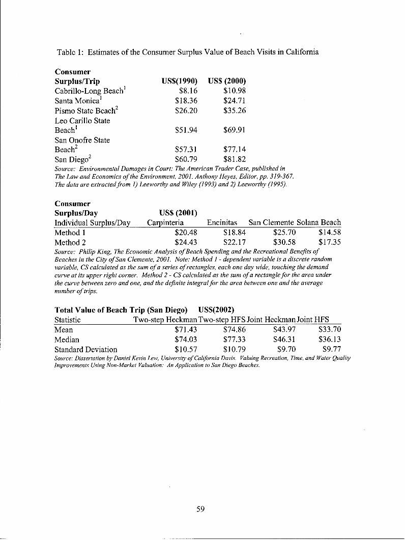
Table 1: Estimates of the Consumer Surplus Value of Beach Visits in California
ConsumerSurplus/Trip US$(1990) US$ (2000)Cabrillo-Long Beach' $8.16 $10.98Santa Monica1 $18.36 $24.71Pismo State Beach 2 $26.20 $35.26Leo Carillo StateBeach' $51.94 $69.91
San Onofre StateBeach 2 $57.31 $77.14
San Diego2 $60.79 $81.82Source: Environmental Damages in Court: The American Trader Case, published inThe Law and Economics of the Environment, 2001, Anthony Heyes, Editor, pp. 319-367.The data are extracted from 1) Leeworthy and Wiley (1993) and 2) Leeworthy (1995).
ConsumerSurplus/Day US$ (2001)Individual Surplus/Day Carpinteria Encinitas San Clemente Solana BeachMethod 1 $20.48 $18.84 $25.70 $14.58Method 2 $24.43 $22.17 $30.58 $17.35Source: Philip King, The Economic Analysis of Beach Spending and the Recreational Benefits ofBeaches in the City of San Clemente, 2001. Note: Method I - dependent variable is a discrete randomvariable, CS calculated as the sum of a series ofrectangles, each one day wide, touching the demandcurve at its upper right corner. Method 2 - CS calculated as the sum of a rectangle for the area underthe curve between zero and one, and the definite integralfor the area between one and the averagenumber of trips.
Total Value of Beach Trip (San Diego) US$(2002)Statistic Two-step Heckman Two-step HFS Joint Heckman Joint HFSMean $71.43 $74.86 $43.97 $33.70Median $74.03 $77.33 $46.31 $36.13Standard Deviation $10.57 $10.79 $9.70 $9.77Source: Dissertation by Daniel Kevin Lew, University of California Davis. Valuing Recreation, Time, and Water QualityImprovements Using Non-Market Vahlation: An Application to San Diego Beaches.
59
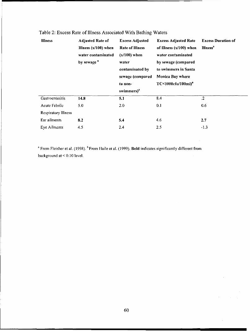
Table 2: Excess Rate of Illness Associated With Bathing Waters
Illness Adjusted Rate of Excess Adjusted Excess Adjusted Rate Excess Duration of
Illness (x/100) when Rate of Illness of Illness (x/100) when Illness'
water contaminated (x/100) when water contaminated
by sewage a water by sewage (compared
contaminated by to swimmers in Santa
sewage (compared Monica Bay where
to non- TC<1000cfu/100ml)a
swimmers)'
Gastroenteritis 14.8 5.1 8.4 .2
Acute Febrile 5.0 2.0 0.1 0.6
Respiratory Illness
Ear ailments 8.2 5.4 4.6 2.7
Eye Ailments 4.5 2.4 2.5 -1.3
a From Fleisher et al. (1998). b From Haile et al. (1999). Bold indicates significantly different from
background at < 0.10 level.
60

Appendix B: Offshore Energy Production in the Gulf ofMexico
Mark J. Kaiser and Allan G. PulsipherLouisiana State University
61
The Impact of Weather and Ocean Forecasting on HydrocarbonProduction and Pollution Management in the Gulf of Mexico
Mark J. Kaiser and Allan G. Pulsipher
Center for Energy Studies, Louisiana State UniversityEnergy Coast & Environment Building
Nicholson Extension Drive, Baton Rouge, LA 70803
Abstract. Weather delay is a common risk in offshore energy production, and theoccurrence of tropical cyclones regularly force operators to shut-down production, ceasedrilling and construction activities, and evacuate personnel. Loop currents and eddies canalso have a serious impact on offshore operations and may delay installation and drillingactivities and reduce the effectiveness of oil spill response strategies. The purpose of thispaper is to describe the manner in which weather and ocean currents impact hydrocarbonproduction and pollution management in the Gulf of Mexico. Physical outcome anddecision models in support of production and development activities and oil spillresponse management are presented, and the expected economic benefits that may resultfrom the implementation of an integrated ocean observation network in the region aresummarized. For effective planning and decision-making, reliable forecasts of weatherand ocean current conditions are required. Improved ocean observation systems areexpected to reduce the uncertainty of forecasting and to enhance the value ofocean/weather information throughout the Gulf region. The source of benefits and thesize of activity from which improved ocean observation benefits may be derived areestimated for energy development and production activities and oil spill responsemanagement.
62
1. Introduction
The Outer Continental Shelf (OCS) 20 of the Gulf of Mexico (GOM) is the mostextensively developed and mature offshore petroleum province in the world. More than40,000 wells have been drilled in the OCS since offshore production began in 1947, andthere are currently over 4,000 active structures in water depths ranging up to 7,000 ft.About 25 percent of the United States domestic oil and gas supply comes from the OCS,and in 2002, OCS lands averaged daily production of about 1.6 million barrels (MMbbl)of oil and 14.5 billion cubic feet (Bcf/d) of natural gas. The Minerals ManagementService estimates that oil production levels will rise to at least 2 MMbbl/d and perhaps ashigh as 2.5 MMbbl/d by 2006, while gas projections through 2006 offer contrastingscenarios 21, with production estimated to range between 11 Bcf/d - 16.4 Bcf/d [1]. Thedeepwater GOM is America's newest production frontier and now accounts for more thanhalf of the Gulf's total oil production [2].
Weather plays a major factor in human activities in the GOM, and extreme weather inparticular, can have an enormous impact on the cost of "doing business." Storms andhurricanes regularly challenge and endanger the coastal community and energyinfrastructure throughout the Gulf region. Every year about 10 storms form over thetropical portions of the Atlantic Ocean, the Caribbean Sea, and the Gulf of Mexico, andabout half of these storms will grow into 75 mph hurricanes (www.nws.gov). Of thesefive hurricanes, two-three are likely to strike the coast of the United States (Table 1,Figure 1). Tropical storms cause damage to physical, economic, biological, and socialsystems, but the severest effects tend to be highly localized.
When a hurricane enters the GOM, oil production and transportation pipelines shut down,crews are evacuated, and refineries along the Gulf coast close. Drilling rigs pull pipe andmove out of the projected path of the storm, if possible, or anchor down, and supplyvessels, commercial ships, and barges may be moved into one of Louisiana's manybayous where they have more protection from the storm. Ocean-going vessels transitinginto or out of the GOM near the time of the event use hurricane forecasts to plot course toavoid the storm. The Louisiana Offshore Oil Port (LOOP), the biggest and onlydeepwater oil port in the country, closes to shipping and flows through on-shore pipelinesare halted. Crude oil from the Gulf to the Midwest via the Capline pipeline, and thegasoline and distillate fuel conduit the Colonial Pipeline, also shut down ahead of thestorm.
Hurricanes are not the only extreme weather event that impacts offshore oil and gasproduction activities. As operators have pushed into deeper waters in the GOM in searchfor oil and gas, the impact of loop currents on operations have become increasinglyproblematic. The Loop Current is an offshoot of the Gulf Stream, a major North AtlanticOcean boundary current located off the east coast of the United States. The loop is
20 The OCS of each coastal state generally begins 3 nautical miles from shore for all but two states - Texas
and Florida - which are 3 marine leagues (9 nautical miles), and extends at least 200 miles through theExclusive Economic Zone.21 Although oil and gas production in the heavily leased shallow waters of the GOM has been steadily
declining, the MMS estimates that there is up to 55 trillion cubic feet (Tcf) of natural gas still available inthe deep shelf areas.
63
formed when the Gulf Stream enters the Gulf of Mexico through the Yucatan Straightsand "loops" through the basin in a clockwise direction before exiting through the Straitsof Florida (Table 2, Figure 2). When the loop exits through the Florida Straight, it oftenbecomes pinched and sheds some of its flow into a separate eddy of warm water whichmigrates backward, southwest across the GOM bringing strong loop current forces intoactive E&P areas [3]. Some oceanographers refer to the Loop Current as the equivalent ofa hurricane beneath the water, and its impact on deepwater installations is increasing asoperators have moved into deeper and more eddy prone areas.
The Loop Current is a persistent feature in the GOM characterized by strong surfacecurrent velocities (2-4 knots) with its position and intensity varying over time. The warm-core eddies that break away from the northern extremity of the Loop Current arecharacterized by intense current velocities which can cause serious impact to offshoreoperations. Typically, two to three eddies form each year. Currents influence rigselection, riser design, many aspects of offshore operational planning, and the design andinstallation of production systems, moorings, subsea components and pipelines. Ofparticular importance is fatigue associated with dynamic response to current loading [4].For effective planning and decision making in the GOM, operators require reliableforecasting of future current conditions.
The National Oceanographic Partnership Program (NOPP) formulated a plan for anIntegrated, Sustained Ocean Observing System (ISOOS) in a 1999 report to Congress [5],intending to move the United States from what is now a largely ad hoc and fragmentedapproach to ocean observation to a coordinated and sustained activity similar to theexisting national weather information system [6-8]. Implementation of ISOOS willrequire investments in infrastructure and ongoing support for new and existingobservation systems in the open and coastal ocean, and the benefits of federal investmentwill depend on the expected costs and benefits of the resulting system. The importance ofa national network of ocean observation systems has recently been reiterated by the U.S.Commission onOcean Policy [9].
The purpose of this paper is to describe the manner in which weather and ocean data isused in planning and decision making activities in offshore energy development andproduction and oil spill response management, and to identify and quantify the expectedeconomic benefits of improved weather/ocean forecasting on these activities. For adescription of the capabilities of each system, the NOAA website (www.csc.noaa.gov)maintains links to each system. The reports [10-15] provide useful summaries ofindividual systems.
The standard economic approach to valuing information requires:
A description of the information being valued and of the uncertainty in thephenomena it describes;
22 A number of initiatives are underway by the academic, government and commercial scientific
community to develop and verify current models of oil and gas basins around the world. The CASE(Climatology and Simulation of Eddies) joint industry project, Oceanweather's WANE (West AfricaNormals and Extremes) joint venture between Fugro and the Nansen Environmental and Remote SensingCenter at the University of Bergen, and the U.S. Navy are all working on advanced ocean current modelingprograms [4].
64
* A model of how this information is used to make decisions;
* A model of how these decisions affect physical outcomes;
* A model of how physical outcomes can be translated into economic outcomes.
User sector representatives were identified to define the base case and improvedinformation scenarios, and then information was obtained regarding the natural variationof the phenomena being described, including critical variables to nowcast/forecast, theforecast horizon, spatial and temporal resolution. A decision model is then sketcheddescribing how users incorporate information into their choices and decisions. Thephysical outcome describes how outcomes result from the decision parameters and thevariation in the natural phenomena. Finally, a simple economic outcome model describeshow the physical outcomes translate into economic changes.
The outline of the paper is as follows. In §2, the methodology of the economicvaluation is presented. In §3-6, the decision, physical outcome, and potentialbenefits of improved observation systems to energy exploration, development, andproduction activities are described, and in §7, the decision, physical outcome andeconomic outcome models related to oil spill response management are discussed.In §8, conclusions complete the paper.
2. Valuation Strategy
The state of knowledge of ocean data is incomplete and uncertain, and so improvedocean/weather observation systems are expected to enhance the value of the informationand create additional network externalities [6]. Weather information is valuable, and tothe extent that improved ocean observation systems can improve the data on whichweather/ocean forecasts is based, is potentially very beneficial to energy productionactivities and pollution management in the GOM.
The potential impact of savings that may be incurred from improved oceanobservation systems was first estimated by Kite-Powell and Colgan in a study focused onthe Gulf of Maine [16]. Kite-Powell and Colgan performed order-of-magnitudeassessments for general categories of benefits using the following methodology:
Step 1. Value activity A that uses and/or is impacted by ocean forecasts, V(A).
Step 2. Assume that the benefit of improved ocean observation systems isexpressed by some small factor, e(A) > 0.
Step 3. Compute the value of improved observation systems in region R,V(R) = Xe(A)V(A).
A
The valuation strategy is based on estimating V(A) from public sources of informationand hypothesizing the value of e(A) for each activity identified. The selection of e(A) ishypothetical but not unreasonable within the framework of the model and the scope of thevaluation. Ideally, it would be desirable to derive the value of e(A) from fundamental dataor to ascertain the cost to achieve a desired level of e(A), but establishing such
65

relationships are beyond the state of knowledge of observation systems. Further, no directlink between e(A) and V(A) can be "derived" and it is difficult to "justify" e(A) on afundamental level. The default condition is to assume e(A) "small" (e.g., 1%, 1 day, etc.),and this is considered a "reasonable," and in all instances, a conservative estimate of theexpected benefits to be incurred.
3. Stages of Offshore Energy Development
A four-stage sequence of activity is generally followed in offshore energydevelopment projects:
1. Exploration,
2. Development,
3. Production, and
4. Decommissioning.
In the exploration stage, areas that are considered to have prospects of containing oil andgas reserves are drilled with exploratory wells and stratigraphic test wells. In thedevelopment stage, the mineral deposit is prepared for commercial production. Thisincludes the acquisition, construction, and installation of facilities to extract, treat, gather,and store the oil and gas. In contrast to a single exploratory well for which drilling canlast anywhere from 2 weeks to 3 months, drilling the wells off a platform can last manymonths and extend over several years. Development activities typically include drillingand equipping development wells and service wells, and the construction and installationof production facilities. The ongoing operation of the facility is considered the productionphase. In production, the oil and gas is gathered, lifted to the surface, treated, processed,and possibly, stored. When the useful life of a production platform is reached, theequipment and structure is removed and the well casing severed and closed below theseabed.
4. Drilling Activities
4.1. Decision Model
Offshore drilling may be subject to significant delays caused by the weather, andweather downtime can play an important factor in the total costs of the operation. Wavesare one of the most obvious environmental concerns for offshore operations andconstitute the primary cause of downtime and reduced operating efficiency. Weatherdowntime can impact drilling operations in various ways; e.g., weather too severe foroperations involving supply boats may lead to delay if stock levels on the rig decline to acritical level; weather may impact anchoring up and moving time; weather may be toosevere for drilling to occur; and extreme weather may result in damaged or lost drillstrings and risers. If operating limits are exceeded because wave heights, ocean currents,or eddies are too strong, drilling operations will be temporarily abandoned and resumedwhen conditions fall within the operating capabilities of the equipment.
66
Safe working conditions for many offshore operations may be approximatelyspecified by the critical values of wind speed and wave height, and for deepwater drillingactivities, current profile, as shown in Table 3. The GOM is a fairly benign operatingenvironment for most of the year, but downtime due to weather can be an importantfactor in determining the total drilling costs, and in the deepwater, usually plays a moresignificant role because of the day rate of the drilling rig. Empirical evidence suggeststhat 1-3% of drilling cost is due to waiting on weather [17], although this is subject tosignificant variation depending on the time of year of drilling activity and the water depthof the operation. In deepwater, floating rigs are able to maintain position over the tops ofwells through a dynamic positioning system that compensates for wind, waves, andcurrents to keep the vessel stationary relative to the seabed.
Drilling activities generally follow three stages:
1. Start limits. Weather must be below these limits before an operation will start (orrestart after abandonment).
2. Suspend limits. Work will be paused if the environment exceeds these limits.Work recommences as soon as weather conditions drop back below the threshold.
3. Abandon limits. Task will be abandoned if these limits are exceeded. Work willnot be restarted until weather conditions fall below the start limits.
The occurrence of a hurricane warning or alarm is enough to disrupt drillingoperations, and a significant amount of operating time can be lost to "false alarms" [ 18-20]. In deepwater operations, loop currents and eddies associated with them are alsocommon phenomena that may damage drilling strings/risers and impact the drillingschedule [21]. In drilling operations, eddies may induce vortex-induced vibrations thatreduce the fatigue life of equipment. Eddies can hold currents of four knots or more at thesurface and extend several hundred meters deep and measure as wide as 250 miles indiameter. The operational limit for diver operations is half a knot or less, whiledeployment of tubulars and risers can usually be safely performed in currents up to 1.5knots.
4.2. Physical Outcome
To a large extent, the impact of severe weather on drilling depends on the choice ofrig the operator has chosen for the operation. Many different rigs can be used to drill anoffshore well and rig selection depends upon factors such as the type of well beingdrilled, water depth and environmental criteria, the type and density of the seabedexpected drilling depth, load capacity, frequency of moves, ability to operate withoutsupport and rig availability.
If weather and environmental conditions are expected to be a problem, thensophisticated all-weather semis can be used to hedge against weather downtime. Theincrease in availability is achieved through the higher capital cost of the equipment;which in turn is passed to the operator in higher day rates. Jack-ups are cheaper but aremore prone to weather delay. The choice is up to the operator: the trade-off is betweendrilling availability and day rate.
67
The cost of deepwater drilling can represent a significant portion of the total fielddevelopment costs, perhaps as much as 20-40% of total costs, and so operators pay closeattention to the environment to minimize the magnitude of the risk. Because of thepotentially catastrophic effect a powerful eddy can have on a drilling riser, it is commonto monitor the approach of an eddy and pull the riser or circulate the stroke pipe beforethe eddy actually reaches the platform. In April 2003, strong eddy currents and tropicalstorm Bill and hurricane Claudette impacted several deepwater operations; e.g., Shell'sNakika was delayed 1 week; Total's Matterhorn TLP was delayed 6 weeks; Heerema'sBalder experienced several delays in BP's Mardi Gras pipeline installation [3].
"Eddy Watch" and "Eddy Net" are monitoring systems operated by Horizon Marine(www.horizonmarine.com) that provides real-time ocean current maps (Figure 2).Horizon Marine's Eddy Watch is a weekly report published since 1984 that containsinformation on eddies in the GOM. The data is gathered through 45 drifting buoysequipped with Argos GPS satellite transmitters that float in the currents and trackmovements. The buoy data is combined with infrared satellite imagery, altimetry andremote sensing to compile the Eddy Watch report. Eddy Net is a real-time, rig-mountedADCP system in 500-800 m water depth installed in 6 sites in the GOM (Figure 3) withplans to have 20 sites by 2005. Operators also directly monitor currents through their ownsite surveys of current meters installed on boats, rigs, and platforms; e.g., Shell uses theADAM system (ADCP Data Acquisition Manager). ChevronTexaco, BP, and Marathonuse ADCP on various active production facilities and drilling rigs.
4.3. Economic Outcome Model
The Joint Association Survey on Drilling Costs estimated that the total cost of drillingin the GOM in 2000 was $4.6 billion [22], and over the past few years, the total annualoffshore drilling cost ranged between $3-5B. If we assume 1-3% of the total drilling costis due to waiting on weather and that improved ocean observation systems can mitigate1% of these costs, the expected annual savings due to improved ocean observation data isestimated to lie between $300,000 and $1.5M.
5. Development Activities
5.1. Decision Model
One of the primary goals in any construction project is predictability, but because ofthe nature and location of the operation, offshore construction activities will always beuncertain and unpredictable. There are numerous independent uncontrollable variables inthe offshore environment, such as adverse sea conditions and weather, availability andperformance of equipment, defects in plans and specifications, and work conditions thatresult in delay, and often, significant financial repercussions. Delay is a common risk inoffshore construction projects and the parties of the contract apportion risks for delaysthat may be encountered. In the case of weather risk, construction contractors willfrequently quote a lump sum (base) bid that includes weather downtime, exceptdowntime due to named tropical storms, for work during the prime season (May 15 toOctober 15).
68
There are a wide variety of construction vessels used in the GOM and contractorsplan their operations using ocean/weather forecast to avoid adverse weather andoperating conditions. Typical offshore construction craft include crane vessels, drillships, dive support vessels, survey vessels, cable lay vessels, pipelay vessels, multi-purpose support vessels, dredging vessels, and trawling vessels. The vessels come in avariety of shapes and sizes, from rectangular barges to jack-ups and semi-submersibles.
Offshore construction vessels differ from merchant ships because they do not tradecargo between ports and their most critical operations and loading conditions occur whileworking on the high seas (and not at the start or end of their voyage). Constructionvessels also differ from passenger ships since they are much stronger and the designstandards have to satisfy a multitude of strict safety regulations.
There are guidelines for marine operations such as barge transportation, platformmating and lift-off, etc. In barge transportation for example, weather forecasts arenormally provided at 12-hour intervals and contain forecasts for the next 24 and 48 hours,with the weather outlook for the coming 3-to-5 day period. Tows are designed towithstand a 10-yea-r return period for extreme environmental conditions for the mostexposed part of the route for the month or months during which the transportation takesplace. For long duration tows passing through areas having different characteristic seastates, the worst sea state for the route is identified and used in the design of the cargo,grillage, and sea fastenings [23, 24]. In installation operations, time-sensitive equipmentsuch as ROVs and heavy lift vessels may not be able to operate in high current.
5.2. Physical Outcome
During construction activities, a moving vessel is installing (or removing) somethingon a fixed seabed, which leads to the requirement that vessel motions be minimized asmuch as possible to maximize the operational window. There are typically two options bywhich major projects are installed and completed offshore: floatover, in which the unit islowered into place from its transportation vessel, or heavy lift, in which the unit is liftedinto place with large vessel-mounted cranes. The transportation and installationlimitations of the construction approaches dictate the size, weight and weight distributionof the modules. The heavy-lift method of installation is able to complete installations inchallenging sea-states but the use of such equipment is also more costly. Lay barges forinstance are designed to operate at different wave heights, allowing the operator tochoose the barge to the sea conditions in the area. The prime risk factor is the weather,and specifically, wave heights. A barge that can operate in 2-m wave height cost about$250,000/day while the cost for a 5-m wave height lay barge cost about $500,000/day.The application of reliable ocean forecasting in pipe laying is obvious. If pipelineinstallation is finished late, or delayed by unexpected ocean conditions, the direct cost ofdelay expressed in terms of the day rates and the opportunity cost of nonproductivestructures and wells is likely to be substantial.
5.3. Economic Outcome Model
Order-of-magnitude savings for construction and transportation activities in the GOMare estimated as follows. With the occurrence of a hurricane event, weather forecasting
69
model improvement is assumed to provide a 10% or more accurate prediction of the
storm path and arrival time saving 3-5 days work time.
(1) Operator Savings - Construction
Assumptions:
"* Activity: 50 installed structures/yr, 50 removed structures/yr
"* Construction activity level at time of hurricane passage: 50% total structures
"* Number of structures in hurricane path: 50% total structures
"* Derrick barge cost: $1 00,000/day
Expected Savings:
(50+50)(0.50)(0.50)(0.10)($100,000/day)(3-5 days) = $0.75-1.25M/yr.
(2) Operator Savings - Supply Vessel
Assumptions:
"* Number of active supply vessels: 500/day
"* Number of supply vessels in hurricane path: 50% total structures
"• Supply vessel cost: $20,000/day
Expected Savings:
(500)(0.50)(0.10)($20,000/day) (3 days) = $1.5-2.5M/yr.
6. Production Activities
6.1. Decision Model
What is considered to be severe weather varies with each platform and drill site.Companies develop emergency procedures for each type of rig and manned platform theyoperate, and there is no standardized shutdown or evacuation procedure in the event of anextreme weather event or disaster. Shut-down and evacuation procedures vary fromcompany to company and depend upon the rig type and design, the location of theoperation, and the behavior of the weather.
The decision to shutdown or evacuate and the actions taken by the crew ensure that noemployees are injured, damage to the operation or rig is minimized, anddrilling/production can be resumed as soon as possible after the event passes. The drillingsuperintendent and marine superintendent establish in writing specific procedures for theoperation, evacuation, and securing of their particular rig or platform in adverse weather.The location and design of the rig determine the actions to be taken. Submersible, jack-upand semisubmersible rigs are usually not moved from location. On submersible rigs, therig is typically moved across from the wellhead to prevent damage, and on jack-up rigs,the hull is jacked up to avoid high seas. On semisubmersible rigs, the drill string hangsoff in the wellhead and the anchors are slackened to reduce tension. If weather is
70
extremely severe and the rig rolls excessively, mud and bulk material may be dumped.Drill ships and drilling barges follow most of the same procedures but may be moved toinland waters out of the storm's path.
The evacuation and shutdown action plan generally follow a well-defined sequence ofactivities:
1. Regional tropical cyclone climatology is reviewed for area of operation.
2. National Hurricane Center analysis/forecast charts are obtained, including surface,upper level, and sea state (wind/wave) charts.
3. Tropical waves, disturbances, and tropical cyclones are located and plotted.
4. The closest point of approach 23 and time to tropical cyclone is calculated.
5. Decisions on the course of action to follow on the latest safe departure time aremade and executed.
6. Actions are reviewed when new meteorological analysis and forecast informationbecomes available.
Approximately 5-7 days before the expected arrival of the hurricane, the evacuation andshutdown action plan is initiated. Storm path, speed, and intensity forecast information istypically supplemented by in-house/consulting meteorologist and/or local weather serviceproviders24. Team leaders, operational managers, and meteorologist meet twice a day toplan and schedule evacuation activities with primary consideration given to the latest safedeparture time for personnel 25.
Operators are responsible for the safety of all personnel on their structures, and 2-5 daysprior to the arrival of the storm, all nonessential personnel are evacuated during daylighthours. Essential personnel are the last to go and are transported to shore after wells areclosed and topside equipment secured 1-2 days before the storm is expected to hit. In the1960's operators considered 3 days the minimum time window to evacuate personnel andshutdown operations, while today with better and more reliable weather forecasting, 1-2days is considered a safe window. Shut down can be performed automatically, in factnearly instantaneously, using automatic control systems on wells where it is deployed,
23 The 1-2-3 Rule of Thumb is the most important aid in assessing "track error," the distance between the
predicted position of a storm's center and its actual position. The 1-2-3 Rules of Thumb is derived from thelatest 10-year average track error associated with hurricanes in the North Atlantic:1-100 mile error radius for 24-hr forecast2-200 mile error radius for 48-hr forecast3-300 mile error radius for 72-hr forecast24 The size of the private/commercial meteorological value added sector is estimated to employapproximately 4,000 people with $400-700M in annual gross receipts [26]. Most of the firms are soleFroprietorships.5 It is possible for crews on manned platforms to bunker down and weather out most hurricanes in the
GOM, but for safety and family concerns, all personnel are usually evacuated. The safety record associatedwith offshore production has been exceptional over the past two decades. The last major event occurredwith Hurricane Juan in 1985, where several rigs and boats capsized and in total nine lives were lostoffshore.
71
and for manned platforms, shut down is performed in stages according to facilityrequirements.
6.2. Physical Outcome
Severe weather procedures vary according to the type of rig [25].
Submersible andjackup rigs
"* On submersible rigs, move back enough from the wellhead to preventwellhead damage, and increase ballast so that high seas will not move the rigoff location.
"• On jackup rigs, jack up the hull to avoid high seas. Jackup rigs are usually notmoved in severe weather.
"* Remove all drill pipe in the derrick on both submersible and jackup rigs.
Semisubmersible rigs
"* Suspend drilling and hang off the drill string in the wellhead before theextreme weather arrives.
"* If waves are expected be extremely large, pull the upper package. Slacken leeanchors to reduce anchor tension on windward anchors.
"* Lay down and secure the cranes.
"• Deballast the rig to allow waves to pass beneath the rig.
"* Apply thrusters to relieve tension on the windward anchors.
"* Keep a constant check on anchor tension.
"• If the upper package was pulled, make sure the station-keeping equipment ismonitoring a beacon attached to the lower package.
"* Make sure that the standby boat is kept downwind or abeam.
"* If the weather is extremely severe and the rig is rolling excessively, dumpmud and bulk material.
For drill ships and barges, most of the above procedures are followed but need to beperformed sooner. Drill ships and drilling barges may be moved out of the path of thestorm and to inland waters out of the storm's range.
Companies transport crews offshore in helicopters, crew boats, and workboats accordingto their operational guidelines. The major environmental parameters in offshoreemergency evacuation are the wind speed and wave height, and safe working conditionsfor many offshore operations may be approximately specified by critical values of theseparameters (recall Table 3). The limiting conditions for the operation of helicopters areusually defined in terms of wind speed (typically 40-50 mph), and visual flight rulesspecify that the operating minimum for single-engine helicopters is a 3-mile visibilitywith a 500-ft ceiling. The minimum operating conditions for multiengine helicopters is a2-mile visibility with a 300-ft ceiling. Wave height must fall below a given threshold
72
(typically 5-8 ft) to ensure safe transfer operations with the crew or workboat.Evacuations are performed in the daytime and the method of evacuation depends on thesea state, distance to shore, climatic conditions, and availability of transportationequipment. Thunderstorm activity will restrict helicopter usage. The number of personnelinvolved in an evacuation depends on the type of structure: a small drilling rig may havea crew less than 10 while a large production platform could have over 100. In the GOM,there are currently about 25,000 offshore workers on any given day.
Some of the large operators in the GOM own a fleet of helicopters and will maintainannual contracts with service boats moored at various offshore production sites. Smalleroperators reserve space on crew boats and helicopters26 subject to availability, but there isusually sufficient capacity to ensure crews are transported in a safe and timely manner.For the planners and managers of evacuation activities, however, work conditions remainstressful and difficult during a hurricane event until all personnel arrive safely on-shore.
The occurrence of an extreme weather event requires operators to decide what facilitiesto shut down and when personnel should be evacuated. Current GOM operatingphilosophy requires the evacuation of all personnel before the latest safe departure timeand the shutdown of most, if not all, production activity. Shutting down production hasan immediate negative economic impact on the operator, but because of the extreme riskinvolved with tropical storms, a "conservative" approach is normally taken in planningactivity. The safety record associated with offshore evacuation has been exceptional over
27the past two decades
6.2. Physical Outcome
Immediately following a storm, the MMS will issue a Notice to Lessees requiringoperators to conduct a Level X (X = I, II, III) survey for a Y-mile corridor around thestorm path; e.g., Level I surveys are a visual inspection from the topside and thecomplexity of the inspection increases with the level specified. Damage can take manyforms [28]:
"* Platforms, caissons, and flare piles can list (lean), topple, or are condemned."* Drilling rigs, barges, and workboats can be grounded or capsize.* Flowlines and pipelines can be damaged by a dragged anchor.* Topsides equipment such as pumps, tank batteries, power generators, etc. may
have water damage.
The damage incurred to a structure translates to a direct economic loss to the operatorsince many are self-insured. Operators, and to a lesser extent, insurers, absorb the cost ofa hurricane, while service companies performing underwater inspections and emergencyrepair and construction and equipment suppliers benefit from the business derived from
26 Typical dayrates for a 34 ft crew boat is $600-800/day, while for a 190 ft crew boat, $2,000-4,000/day.Typical helicopter rates are $1,000-1,500/hr. A crew boat can transport up to 90-130 people; a helicopter upto 25 depending on its size. Unscheduled, weather-related evacuations add approximately $10,000 perproduction facility and $50,000 per drilling rig over and above normal transportation cost [21].7 The last major event occurred with Hurricane Andrew in 1992, where 164 structures were destroyed,
including 22 major platforms [27].
73
the event. The cost associated with a hurricane and borne by operators is thus "balanced"to some extent by the economic stimulus that follows in the wake of the storm.
Starting up production and re-pressurizing wells after shutdown can beproblematic and usually takes a few days, especially when inspections need to beperformed. Engineers must spend time inspecting pipes, pumps, and process facilitiesbefore the spigots are reopened. Wells that have been shut off can suffer from temporaryshifts in the underground pressure, reducing initial output for weeks or months. In otherfields, shutting down can help rebuild pressure and enhance production rates. The successof start-up operations depend in large measure on the damage caused by the storm, thecharacteristics of the geologic formation, and the complexity of the wellbores. Since mostGOM crude oil is light and in primary production, start up activities are mostlyperformed without consequence, and assuming no storm damage, fixed structures maycome back on-line within 48-72 hr of evacuation. Individual wells may be off productionfor several weeks or even months. Floating production systems, which operate in thedeep waters of the GOM and where hydrates may form, may take up to one week toresume production.
6.3. Economic Outcome Model
A company will typically include anywhere from 3-5 days of weather-relatedproduction losses each year in their business plans to account for the uncertainty ofweather. Operators incur the cost associated with deferred production, evacuation cost,damage assessment, and facility repair, if any, prior to the resumption of production.Most of these costs, with the exception of deferred production and human lifeconsequences, cannot be mitigated or reduced, since offshore production facilities cannotbe moved out of the path of the storm or otherwise avoid the storm's impact.
The direct cost involved with a hurricane event includes shut-down cost, C1;evacuation cost, C2; downtime cost, C3; damage assessment cost, C4; facility repair cost,C5; and start-up cost, C6. Improved ocean observation systems are expected to allowsome of these costs to be reduced, delayed, or possibly avoided - in particular C2 and C3- although it is clear that no observation system cannot mitigate the actual damage of theevent unless boats and drilling vessels are moved out of the track of the storm thatotherwise would not have been moved. Shut-down and start-up cost (C1, C6), damageassessment cost (C4), and facility repair (C5) depend on the track and strength of thestorm and the amount of damage inflicted and are not influenced by improved oceanobservation systems except in the development design stage28.
Hurricane motion is controlled by the state of the surrounding atmosphere, andforecasts based upon more accurate and timely measurements of that state are themselvesmore accurate. If the forecast associated with a hurricane event can be improved, then
28 The optimal design of an offshore facility, especially floating production facilities in the deepwater
GOM, requires knowledge of the response of the structure to environmental loading, which in turn, iscritically dependent on the acquisition of reliable data on current profile and wave height. It is important toassess seasonal and inter-annual variability in dynamic conditions, but it is seldom possible or cost-effective to undertake multiple-year site-specific measurement programs in support of field development.
74
production can stay on-line a greater period of time without sacrificing safety orenvironmental considerations, and in the best case, perhaps not shutdown at all. Order-ofmagnitude estimates for evacuation and lost production savings are provided as follows.
(1) Operator Savings - Evacuation
Assumptions:
"* Manned platforms in hurricane path: 750
"* Rigs in hurricane path: 100
"• Evacuation cost: $10,000/platform, $50,000/rig
"* Weather forecasting model improvement: 10-20% more accurate predictionon hurricane path/zone to avoid evacuation
Expected Savings:
(750)(0.10-0.20)($10,000/platform) + (100)(0.10-0.20)($50,000/rig) = $1.25-2.5M/yr
(2) Operator Savings - Lost production
Assumptions:
"* Net income margin per BOE: $5/BOE
"• One-half of GOM production shut-in: 1.5 MMBOE/day
"• Weather forecasting model improvement: 0.5-1 day continued production
Expected Savings:
(1.5 MMBOE/day)($5/BOE) = $3.8-7.5M/yr
7. Oil Spill Management and Response
7.1. Decision Model
The risk of oil spills arise from activities associated with the exploration,development, production, and transportation of offshore oil and gas resources, as well asfrom the transport of oil across the ocean to port facilities [29, 30]. During the 1970s andearly 1980s most of the crude oil and products moved by water was associated withinland barges or coastwise movement between U.S. production/processing andconsumption regions. By the mid-1980s, waterborne commerce of foreign imports ofcrude oil and petroleum production exceeded coastwise transportation, and today iscompletely dominated by foreign imports.
Oil spills in coastal waters are especially damaging and clean up can be veryexpensive. The Oil Pollution Act of 1990 [31 ] requires that response activities deal withthe legal constraints and interest of various political entities as it attempts to minimizeecological damage and the quality of human life. Better knowledge of wind and watercurrents will assist in the management and clean up of oil spills.
75
Four factors influence oil spill response: the type of oil (e.g., heavy crude, distillatefuel, etc.); the amount of oil spilled; the spill conditions, which are described by seatemperature, ocean current, wind and weather conditions; and proximity to ecologicallysensitive areas. Once notice has been received that a spill has occurred all of these factorsare assessed to determine the spill response.
Information to support operational decisions during an oil spill is provided through avariety of sources. Typically, decision-making is aimed at supporting a "minimumregret" as opposed to a "maximum win" strategy [ 14]. In a "maximum win" strategy, thebest estimates of wind, currents, and the initial distribution of the pollutant is collectedand the resulting forecast taken as the threat. A "minimum regret" strategy on the otherhand uses whatever analysis techniques are available as input data. The situation unitpresents the command with not only the "best guess" of where the oil will go but alsowith alternate possibilities that might present a significant threat. Reliable near-time dataon the wind and wave conditions is essential for good decision-making.
7.2. Physical Outcome
Oil spill response is site specific and occurs within a complex, dynamic, anduncertain environment. The environmental effects of oil spills vary widely depending onfactors such as the amount and type of oil spilled, weather conditions, the location of thespill relative to natural resources, the quality and sensitivity of effected resources,seasonal factors, and the thoroughness and speed of cleanup and restoration efforts(Figure 4).
Clean up operations employ one or more methods such as mechanical systems,chemical dispersants, burning, and bioremediation depending on prevailing spillconditions. Timing is critical to effective clean up. Floating oil spreads rapidly, and aslow response may allow oil to spread over a large area so that boom is not effective incontainment. Floating oil also emulsifies as it mixes with water lending treatment withdispersants ineffective after a given time window has passed.
7.3. Economic Outcome Model
There are many social costs associated with an oil spill. Many costs can be measuredas direct economic cost such as the cost of clean up, while indirect cost such as damageor harm to wildlife cannot be measured in a market transaction. Indirect social costs aretypically valued using "willingness-to-pay" techniques or an assessment of the loss inconsumer surplus. The estimated unit cost of a barrel of oil spilled or reaching shoreacross the OCS planning areas is summarized in Table 4 [32]. The total estimated cost forthe GOM region is assumed to range between $(888, 1445) per barrel of oil spilled.
The number of spills in the U.S. Coast Guard District 8, which includes Texas,Louisiana, Mississippi, Alabama, and the Florida panhandle, and the volume of spills isshown in Table 5. Roughly one half of the volume spilled came from tank vessels, and60% of the volume involved crude or heavy oil. The 8th District was responsible fornearly 40% of the spills and 38% of the total volume across the United States. Elevenpercent of the total volume of oil spill occurred in the open ocean (12-200 miles), whichwould normally not realize a significant improved response with enhanced oceanforecasting.
76
The impact of a 1% improvement in oil spill response is estimated to result in thefollowing cost savings:
(74,000 bbl/yr)$(888/bbl, 1445/bbl)(1-0.11 )(0.01 )=$(0.58M/yr, 0.95M/yr).
8. Conclusion
Oil and gas technological advancements over the past two decades have beenremarkable, but no matter how ingenious, operators still cannot overcome extremeweather events. Weather information is valuable, and to the extent that improved oceanobservation systems can improve the data on which weather/ocean forecasts is based, ispotentially very beneficial to energy production and pollution management in the GOM.Primary applications of ocean observation data are to provide nowcasts/forecasts ofweather, wind speed, surface wave, current, and general circulation patterns. Order ofmagnitude benefits derived from ocean observation systems to energy related activities inthe GOM are conservatively estimated to range between $8.3-15.3M (Table 6). Theactual benefits derived are expected to be a positive multiple of this factor.
AcknowledgementThe authors would like to acknowledge helpful discussions held with thefollowing personnel: Ken Schaudt, Marathon; Norman Guinasso, Jr., Texas A&MUniversity; Robert Martin, Texas General Land Office; Patrick Michaud, ConradBlucher Institute for Surveying and Science; Mark Luther, University of SouthFlorida; Greg Stone, Louisiana State University; Cort Cooper, Paul Versowsky,Max Regan, Sandy Furr, ChevronTexaco; David Epps, BP, Allan Alrady, J. RayMcDermott; Charlie Colgan, University of Maine; Hauke Kite-Powell, WoodsHole Oceanographic Institution.
This paper was prepared on behalf of the National Oceanographic PartnershipProgram, Office of Naval Research. The opinions, findings, conclusions, orrecommendations in this paper are those of the authors, and do not necessarilyreflect the views of the Office of Naval Research. Funding for this research wasprovided in part through the Office of Naval Research.
ReferencesMelancon J.M., R. Bongiovanni, and R.D. Baud, Gulf of Mexico outercontinental shelf daily oil and gas production rate projections from 2001through 2005, OCS Report MMS 2001-044, U.S. Department of the Interior,Minerals Management Service, New Orleans, May 2001.
Baud, R.D., R.H. Peterson, C. Doyle, and E. Richardson, "Deepwater Gulf of
77
Mexico: America's emerging frontier," OCS Report MMS 2002-022, U.S.Department of the Interior, Minerals Management Service, Gulf of MexicoRegion, New Orleans, 2002.
[3] DeLuca, M., "Current affairs," Offshore Engineer, 29(2), 20-22, February 2004.
[4] Szabo, D., R. Stephans, and R. Smith, "Subsea current analysis evolves,"Hart's E&P, 78(12), 36-37, December 2003.
[5] National Oceanographic Partnership Program (NOPP), "Toward a U.S. planfor an integrated, sustained ocean observing system," A report prepared onbehalf of the National Ocean Research Leadership Council, Washington, D.C.,1999.
[6] Adams, R., M. Brown, C. Colgan, N. Flemming, H. Kite-Powell, B. McCarl, J.Mjelde, A. Solow, T. Teisberg, and R. Weiher, The Economics of SustainedOcean Observation: Benefits and Rationale for Public Funding, WashingtonD.C.: National Ocean and Atmospheric Administration and Office of NavalResearch, 2000.
[7] National Oceanographic Partnership Program (NOPP), Ocean ResearchAdvisory Panel (ORAP), "An integrated ocean observing system: A strategy forimplementing the first steps of a U.S. plan," Washington, D.C., December1999.
[8] Ocean U.S., "An integrated and sustained ocean observation system (IOOS)for the United States: Design and implementation", Arlington, VA, 2002.
[9] "Preliminary Report of the U.S. Commission on Ocean Policy - Governor'sDraft," Washington, D.C., 2004. Available athttp://www.oceancommission.gov.
[10] Michaud, P.R., C. Thurlow, and G.A. Jeffress, "Collection and dissemination ofmarine information from the Texas Coastal Ocean Observation Network," U.S.Hydrographic Conference Proceedings, Hydrographic Society SpecialPublication No. 32, Norfolk, Virginia, 1994, 168-173.
[11] Blaha, T., et. Al, "Gulf of Mexico ocean monitoring system," Oceanography,13 (2), 10-17, 2000.
[12] Cole, R., R. Weisberg, J. Donovan, C. Merz, R. Russell, V. Subrmanian, andM. Luther, "The evolution of a coastal monitoring system," Sea Technology,February 2003, 24-3 1.
[13] Kelly, F.J., N.L. Guinasso, Jr., L.L. Lee III, G,F, Chapline, B.A. Magnell, andR.D. Martin, Jr., "Texas Automated Buoy System (TABS): A public resource,"Proceedings of the Oceanology International 1998 Exhibition and Conference,Brighton UK, 1 (1998), 103-112.
[14] Martin, R.A., F.J. Kelly, L.L. Lee III, and N.L. Guinasso, Jr., "TexasAutomated Buoy System (TABS): Real-time currents for oil spill response,"Proceedings of the 1997 International Oil Spill Conference, April 7-10, 1997,
78
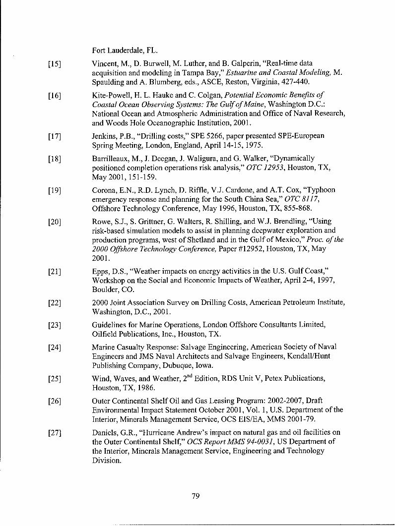
Fort Lauderdale, FL.
[15] Vincent, M., D. Burwell, M. Luther, and B. Galperin, "Real-time dataacquisition and modeling in Tampa Bay," Estuarine and Coastal Modeling, M.Spaulding and A. Blumberg, eds., ASCE, Reston, Virginia, 427-440.
[16] Kite-Powell, H. L. Hauke and C. Colgan, Potential Economic Benefits ofCoastal Ocean Observing Systems: The Gulf of Maine, Washington D.C.:National Ocean and Atmospheric Administration and Office of Naval Research,and Woods Hole Oceanographic Institution, 2001.
[17] Jenkins, P.B., "Drilling costs," SPE 5266, paper presented SPE-EuropeanSpring Meeting, London, England, April 14-15, 1975.
[18] Barrilleaux, M., J. Deegan, J. Waligura, and G. Walker, "Dynamicallypositioned completion operations risk analysis," OTC 12953, Houston, TX,May 2001, 151-159.
[19] Corona, E.N., R.D. Lynch, D. Riffle, V.J. Cardone, and A.T. Cox, "Typhoonemergency response and planning for the South China Sea," OTC 8117,Offshore Technology Conference, May 1996, Houston, TX, 855-868.
[20] Rowe, S.J., S. Grittner, G. Walters, R. Shilling, and W.J. Brendling, "Usingrisk-based simulation models to assist in planning deepwater exploration andproduction programs, west of Shetland and in the Gulf of Mexico," Proc. of the2000 Offshore Technology Conference, Paper #12952, Houston, TX, May2001.
[21] Epps, D.S., "Weather impacts on energy activities in the U.S. Gulf Coast,"Workshop on the Social and Economic Impacts of Weather, April 2-4, 1997,Boulder, CO.
[22] 2000 Joint Association Survey on Drilling Costs, American Petroleum Institute,Washington, D.C., 2001.
[23] Guidelines for Marine Operations, London Offshore Consultants Limited,Oilfield Publications, Inc., Houston, TX.
[24] Marine Casualty Response: Salvage Engineering, American Society of NavalEngineers and JMS Naval Architects and Salvage Engineers, Kendall/HuntPublishing Company, Dubuque, Iowa.
[25] Wind, Waves, and Weather, 2nd Edition, RDS Unit V, Petex Publications,Houston, TX, 1986.
[26] Outer Continental Shelf Oil and Gas Leasing Program: 2002-2007, DraftEnvironmental Impact Statement October 2001, Vol. 1, U.S. Department of theInterior, Minerals Management Service, OCS EIS/EA, MMS 2001-79.
[27] Daniels, G.R., "Hurricane Andrew's impact on natural gas and oil facilities onthe Outer Continental Shelf," OCS Report MMS 94-003 1, US Department ofthe Interior, Minerals Management Service, Engineering and TechnologyDivision.
79

[28] Manning, M.R. and M. Sparks, "Fixed platform inspection process: aregulatory perspective," OTC 13243, 579-587, Offshore TechnologyConference, Houston, TX, April 30-May 3, 2001.
[29] National Research Council, Oil in the Sea IX." Inputs, Fates, Effects, OceanStudies Board and Marine Board, National Academy Press, Washington, D.C.,2002.
[30] National Research Council, Oil Spill Risks from Tanks Vessel Lightering,Washington, D.C., National Academy Press, Washington, D.C., 1998.
[31] Ketkar, K.W. "The oil pollution act of 1990: A decade later," Spill Science andTechnology Bulletin, 2002, 7(2): 45-52.
[32] Estimating the Environmental Cost of OCS Oil and Gas Development andMarine Oil Spills: A General Purpose Model. Vol. I - Economic Analysis ofEnvironmental Cost, U.S. Department of the Interior, Minerals ManagementService, OCS Study MMS 91-043, June 1991.
80
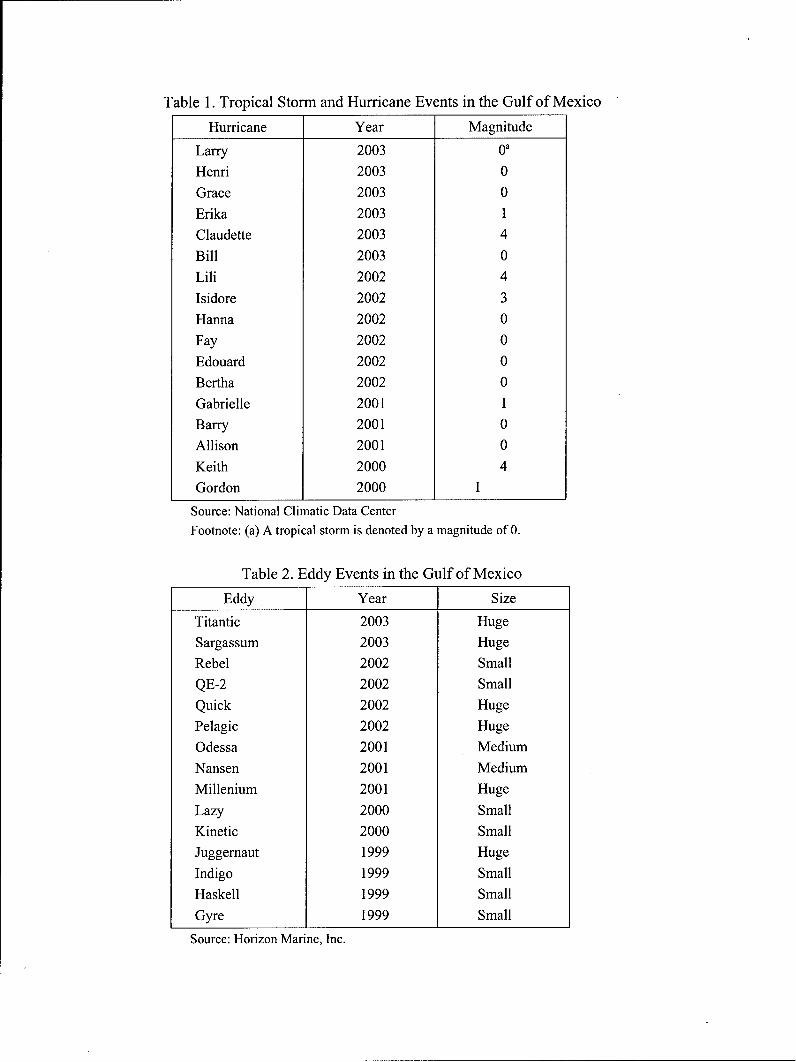
Table 1. Tropical Storm and Hurricane Events in the Gulf of Mexico
Hurricane Year Magnitude
Larry 2003 0a
Henri 2003 0
Grace 2003 0
Erika 2003 1
Claudette 2003 4
Bill 2003 0
Lili 2002 4
Isidore 2002 3
Hanna 2002 0
Fay 2002 0
Edouard 2002 0
Bertha 2002 0
Gabrielle 2001 1
Barry 2001 0
Allison 2001 0
Keith 2000 4
Gordon 2000 1
Source: National Climatic Data CenterFootnote: (a) A tropical storm is denoted by a magnitude of 0.
Table 2. Eddy Events in the Gulf of Mexico
Eddy Year Size
Titantic 2003 Huge
Sargassum 2003 Huge
Rebel 2002 Small
QE-2 2002 Small
Quick 2002 Huge
Pelagic 2002 Huge
Odessa 2001 Medium
Nansen 2001 Medium
Millenium 2001 Huge
Lazy 2000 Small
Kinetic 2000 Small
Juggernaut 1999 Huge
Indigo 1999 Small
Haskell 1999 Small
Gyre 1999 Small
Source: Horizon Marine, Inc.
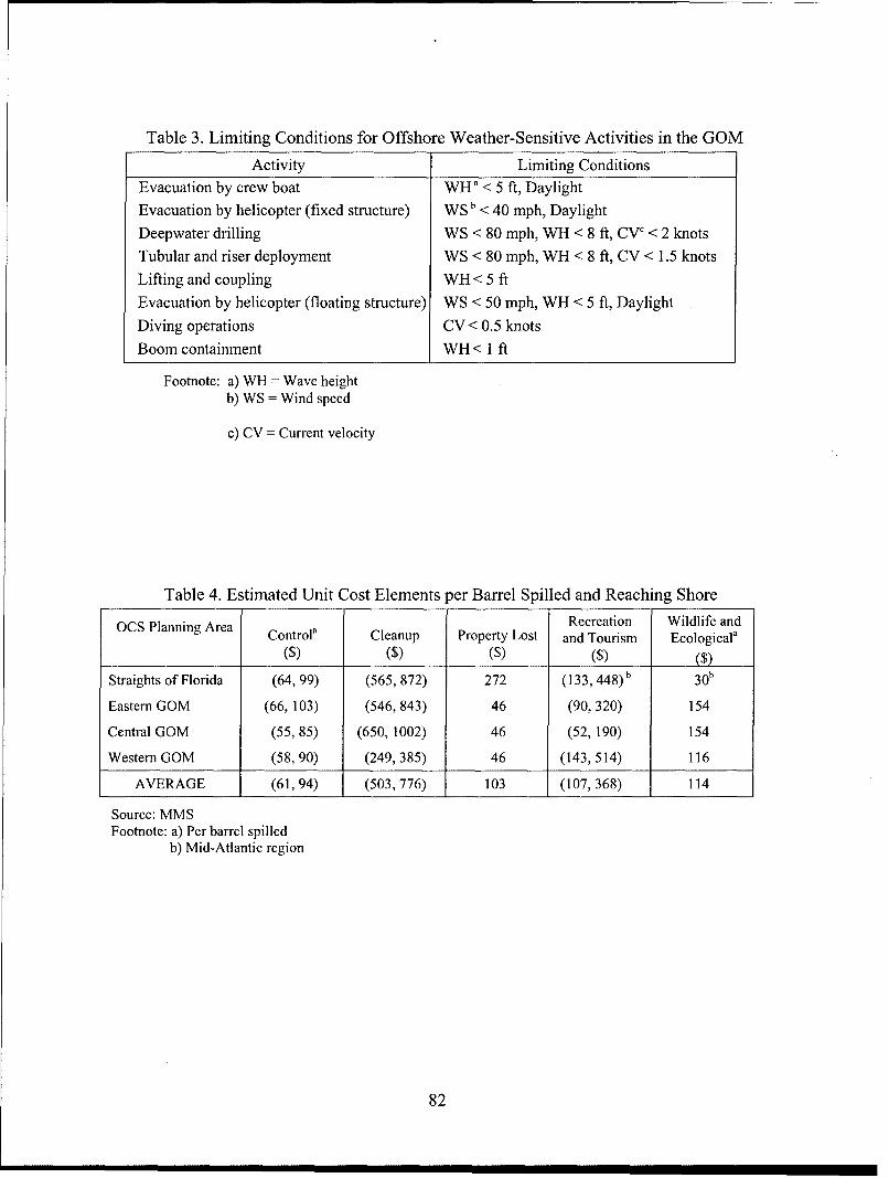
Table 3. Limiting Conditions for Offshore Weather-Sensitive Activities in the GOM
Activity Limiting Conditions
Evacuation by crew boat WH a < 5 ft, Daylight
Evacuation by helicopter (fixed structure) WS b <•40 mph, Daylight
Deepwater drilling WS < 80 mph, WH < 8 ft, CVc < 2 knots
Tubular and riser deployment WS < 80 mph, WH < 8 ft, CV < 1.5 knots
Lifting and coupling WH< 5 ftEvacuation by helicopter (floating structure) WS < 50 mph, WH < 5 ft, Daylight
Diving operations CV < 0.5 knots
Boom containment WH< 1 ft
Footnote: a) WH = Wave heightb) WS = Wind speed
c) CV = Current velocity
Table 4. Estimated Unit Cost Elements per Barrel Spilled and Reaching Shore
Recreation Wildlife andOCS Planning Area Controla Cleanup Property Lost and Tourism Ecologicala
($) ($) ($) ($) $Straights of Florida (64, 99) (565,872) 272 (133, 4 4 8 )b 3 0 b
Eastern GOM (66, 103) (546, 843) 46 (90, 320) 154
Central GOM (55, 85) (650, 1002) 46 (52, 190) 154
Western GOM (58,90) (249,385) 46 (143,514) 116
AVERAGE (61,94) (503,776) 103 (107,368) 114
Source: MMSFootnote: a) Per barrel spilled
b) Mid-Atlantic region
82
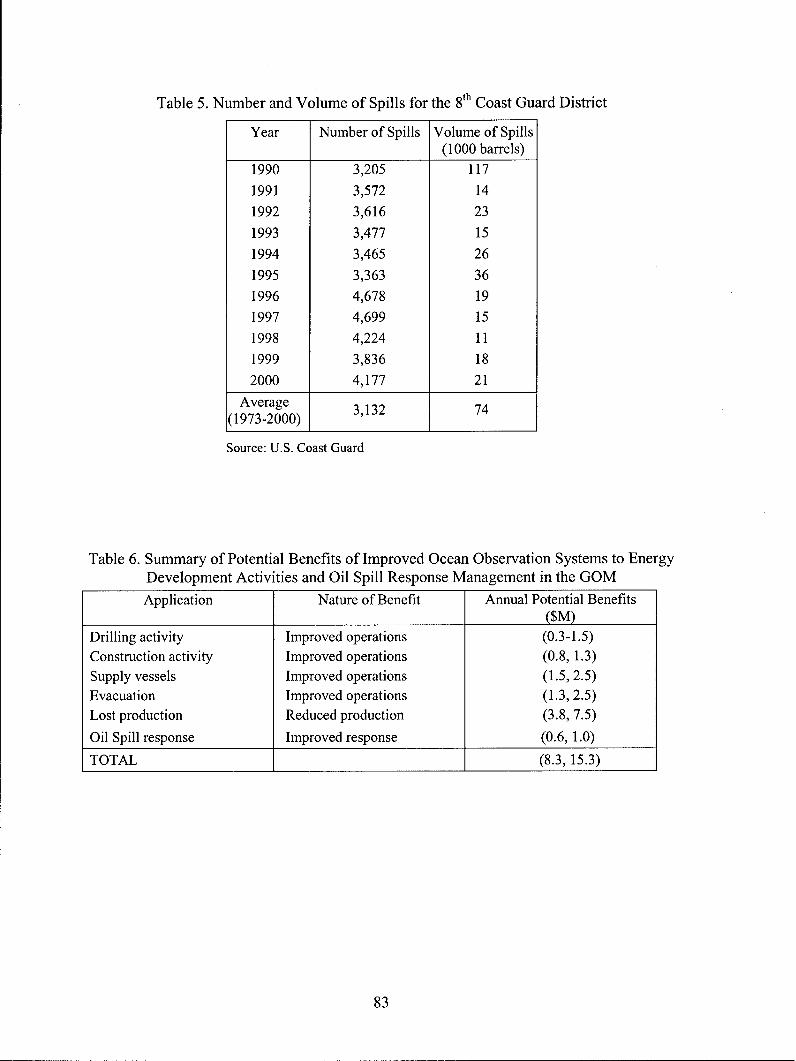
Table 5. Number and Volume of Spills for the 8h Coast Guard District
Year Number of Spills Volume of Spills(1000 barrels)
1990 3,205 117
1991 3,572 14
1992 3,616 23
1993 3,477 15
1994 3,465 26
1995 3,363 36
1996 4,678 19
1997 4,699 15
1998 4,224 11
1999 3,836 18
2000 4,177 21
Average 3,132 74(1973-2000)
Source: U.S. Coast Guard
Table 6. Summary of Potential Benefits of Improved Ocean Observation Systems to EnergyDevelopment Activities and Oil Spill Response Management in the GOM
Application Nature of Benefit Annual Potential Benefits($M)
Drilling activity Improved operations (0.3-1.5)Construction activity Improved operations (0.8, 1.3)Supply vessels Improved operations (1.5, 2.5)Evacuation Improved operations (1.3, 2.5)Lost production Reduced production (3.8, 7.5)
Oil Spill response Improved response (0.6, 1.0)
TOTAL (8.3, 15.3)
83
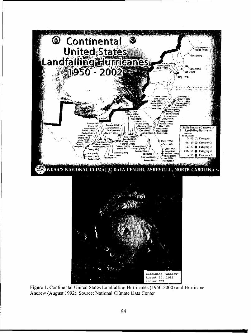
ContinentalUite dStates •
lee~ tQý.' - 0
andfallurricane "Andrew"si
'.1054~ U192 -120
Gab.August 25, 1992 ~
Figure 1. Continental United States Landfalling Hurricanes (1950-2000) and HurricaneAndrew (August 1992). Source: National Climate Data Center
84
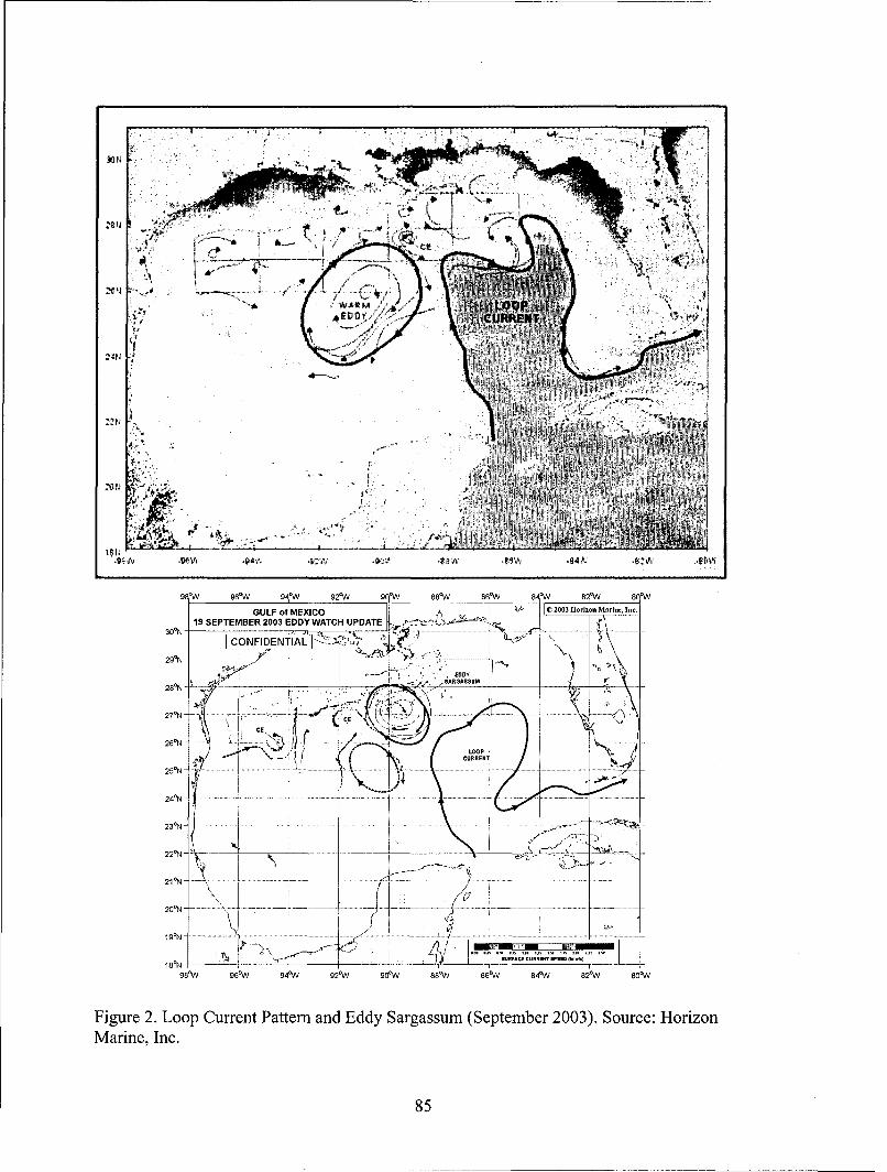
X4N
• .. " .,
00
0;111 -9511 701 4L, 4"'J4- I
9EW 1w AJ 9'ý%V 9;*w 9'w 88G*w_ _8qoA? 8W 8 8W
GULF of MEXICO C 2003 Moz nMarint, lnc.
19 SEPTEMBER 2003 EDDY WATCH UPDATE i
CONFIDENTIAL -- _
29'N 2~EDDY
28_________N__ i.,.ARGASSUM-
27*N
21 0 N. . ... ..-. .-.--. . . .-. .
CET
. .................. . -- ....................
.5. -. ,. ....... .. - . .... . ........ ." -.21 *N -_ - - -... ......------
981W 961W 94•V 92°W 90*W 88W 86VW 840
W 82cW 801W
Figure 2. Loop Current Pattern and Eddy Sargassum (September 2003). Source: HorizonMarine, Inc.
85
IHORI'ZON MNAWINE E~YE__________INC -f D N T
EddyNet Active Data Member SitesMove mouse ever sites on chart below for site info Click on sites to view data
29eN . ...........
2 8 ° N . .. . ................ ...... . .. . . . . . . .! ......... .: ... . .. . ......- • I ................. . . . . .... . . .. .
• oi
0:027 0
2 6 ° N .. . . .. . . .... . . . . . . . . . . . ... . . . . . . . . . . .. . . . . . . . . . .. . . . . . . . . . . . . . . . . . . . . . . . . . . . . .. . . . . . . . ... .. . . . . . . .. . . . . . ... . . L
26'N ,'•, •°• • "''B .. . .............. ............. ........... ......
JFeb 29,2004 1253,3e4 leve Cte S ;tl 0 52 mj
940
W 93°W 921W 91°W 90W 891W 881W
Figure 3. EddyNet Data Collection Sites. Source: Horizon Marine, Inc.
86
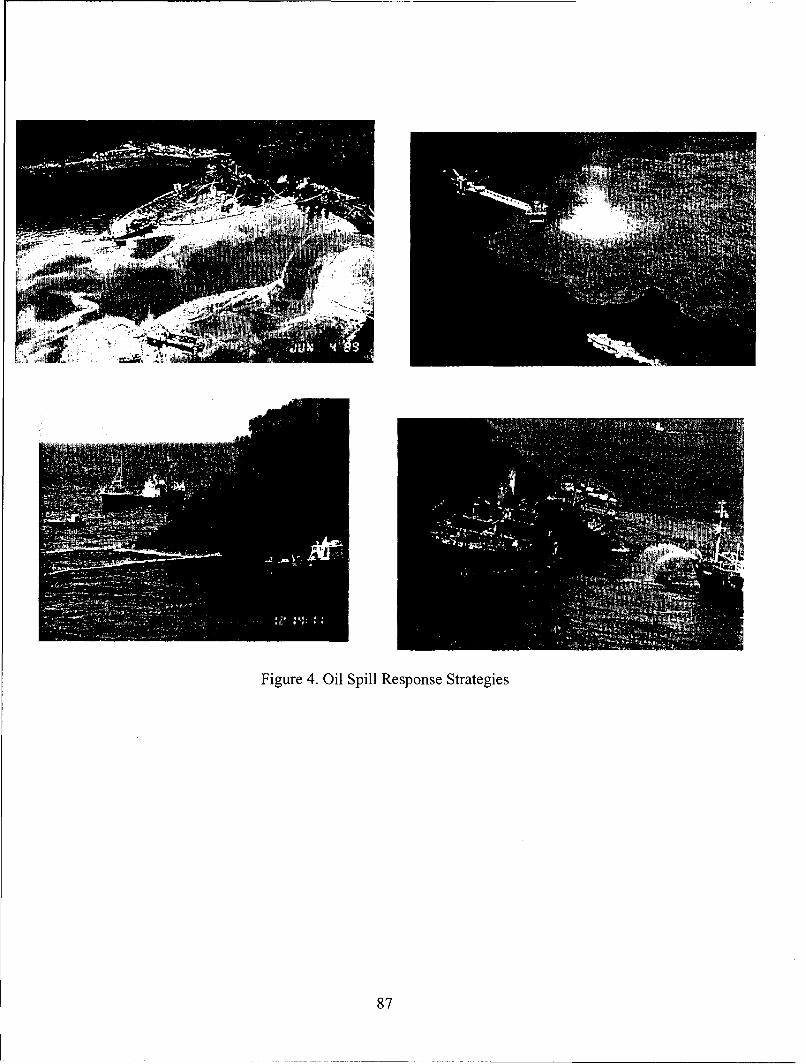
I '~.'.~~ ~ ~ ~ .-
Figure 4. Oil Spill Response Strategies
87

88
Appendix C: Commercial Fisheries in Alaska and the PacificNorthwest
Katharine F. Wellman and Marcus Hartley
89
The Benefits of Enhanced Coastal Ocean Observing Systems:Commercial Fishing in the Alaska Region
Katharine F. Wellman, PhD&
Marcus HartleyNorthern Economics, Inc.
June 27, 2004
Introduction
Alaskan commercial fisheries can be expected to realize benefits from enhancements to theAlaska Ocean Observing System (AOOS). We have identified and attempted to quantifypotential benefits in three areas:
1) Increased harvests
2) Avoidance of overfishing
3) Enhanced business planning
In working towards an assessment of the value of improved coastal ocean observing systems(COOS) to the commercial fisheries of the Alaska region we have found that the use ofCOOS data in research, stock assessment and ultimately fisheries management variesconsiderably from fishery to fishery. As such we have generated a case study approach wherewe look at 3 specific Alaska fisheries. These include: (1) Bering Sea and Gulf of Alaskagroundfish; and (2) Kodiak king crab and (3) Bristol Bay salmon. These case studies offer aqualitative discussion of the current and optimal COOS information scenario, decision-making and physical outcomes and a quantitative analysis of economic outcomes based onplausible scenarios. All assumptions and limitations to the economic assessment of thevalue of improved COOS are stated explicitly.
The analysis and final conclusions of this report were generated using information providedthrough interviews with Directors of the Alaska Ocean Observing System (AOOS) andNorthwest Association of Networked Ocean Observing Systems (NANOOS) and over 25biologists, oceanographers, fisheries managers, and fishers. We also relied on scientificstudies, North Pacific Fisheries Management Council Stock Assessment Fishery Evaluationreports, and relevant secondary literature (please see literature cited section).
Overview of Commercial Fisheries in Alaska
This section provides a general overview of the commercial fisheries in Alaska anddocuments the importance of Alaska fisheries within the US. It provides a summary tableshowing the five major fisheries by species in Alaska and goes on to provide additionaldetails for groundfish, salmon and crab, the top three fisheries by weight and value. Thesethree fisheries are likely to benefit most from an enhanced ocean observing program.
90
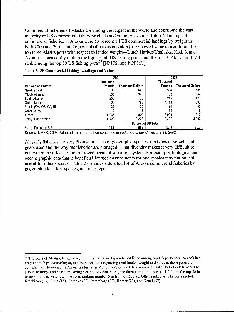
Commercial fisheries of Alaska are among the largest in the world and contribute the vastmajority of US commercial fishery products and value. As seen in Table 7, landings ofcommercial fisheries in Alaska were 53 percent all US commercial landings by weight inboth 2000 and 2001, and 26 percent of harvested value (or ex-vessel value). In addition, thetop three Alaska ports with respect to landed weight-Dutch Harbor/Unalaska, Kodiak andAkutan--consistently rank in the top 6 of all US fishing ports, and the top 10 Alaska ports allrank among the top 50 US fishing ports [NMFS, and NPFMC].
Table 7. US Commercial Fishing Landings and Value
2001 2002Thousand Thousand
Regions and States Pounds Thousand Dollars Pounds Thousand DollarsNew England 635 646 584 685Middle Atlantic 835 347 702 342South Atlantic 200 176 215 173Gulf of Mexico 1,606 798 1,716 693Pacific (WA, OR, CA, HI) 24 55 24 52Great Lakes 19 18 18 16Alaska 5,036 870 5,066 812Total, United States 9,492 3,228 9,397 3,092
Percent of US TotalAlaska Percent of US 53.1 26.9 I 53.9 26.2Source: NMFS, 2003. Adapted from information contained in Fisheries of the United States, 2002.
Alaska's fisheries are very diverse in terms of geography, species, the types of vessels andgears used and the way the fisheries are managed. That diversity makes it very difficult togeneralize the effects of an improved ocean observation system. For example, biological andoceanographic data that is beneficial for stock assessments for one species may not be thatuseful for other species. Table 2 provides a detailed list of Alaska commercial fisheries bygeographic location, species, and gear type.
29 The ports of Akutan, King Cove, and Sand Point are typically not listed among top US ports because each has
only one fish processor/buyer, and therefore, data regarding total landed weight and value at these ports areconfidential. However, the American Fisheries Act of 1998 opened data associated with BS Pollock fisheries topublic scrutiny, and based on Bering Sea pollock data alone, the three communities would all be in the top 50 interms of landed weight with Akutan ranking number 5 in front of Kodiak. Other ranked Alaska ports includeKetchikan (14), Sitka (15), Cordova (20), Petersberg (22), Homer (29), and Kenai (37).
91

Table 8. Major Commercial Fisheries in Alaska
Region FisherySoutheast Troll Fisheries for King and Silver SalmonAlaska-10 Wild Seine Fisheries for Pink and Chum SalmonFisheries Hatchery Seine Fisheries for Pink and Chum Salmon
Statewater Longline Fisheries for SablefishFederal Water Longline Fishery for SablefishLongline Fishery for HalibutSitka Herring Fishery (and possibly other herring fisheries)Southeast AK King Crab FisheriesShellfish Dive Fisheries (Geoduck, Oyster, Urchin, Sponge)Oyster and Mussel Mariculture Fisheries
Prince William Wild Seine Fisheries for Sockeye, Silver and Pink SalmonSound and Hatchery Fisheries for Sockeye, Silver and Pink SalmonCook Inlet- Drift Gillnet Fisheries for King, Sockeye, and Silver Salmon9 Fisheries Set Gillnet Fisheries for King, Sockeye, and Silver Salmon
Statewater Longline Fisheries for SablefishFederal Water Longline Fishery for SablefishLongline Fishery for HalibutPWS Herring FisheryOyster and Mussel Mariculture Fisheries
Central and Trawl Fisheries for Pollock, Pacific Cod, Rockfish, Deep- & Shallow-waterWestern Gulf of FlatfishAlaska- Federal Water Longline Fishery for Sablefish10 Fisheries Longline Fishery for Halibut
Statewater Pot and Jig Fisheries for Pacific CodKodiak Seine Fisheries for Sockeye and Pink SalmonKodiak Setnet Fisheries for Sockeye SalmonChignik Seine Fisheries for Sockeye and Pink SalmonAlaska Peninsula Seine Fishery for Sockeye, Pink, Chum, and SilverSalmonAlaska Peninsula Drift Fishery for SockeyeAlaska Peninsula Setnet Fishery for Sockeye
Bering Sea and Trawl Fisheries for Pollock, Pacific Cod, Atka Mackerel, Rockfish, Flatfish,Aleutian Islands- including fisheries off Adak for Pollock and Pacific Cod6 Fisheries Federal Water Longline Fishery for Pacific Cod
Longline Fishery for HalibutStatewater Pot and Jig Fisheries for Pacific CodPot Fisheries for Red King Crab, Opilio Crab in Bering Sea and PribilofsPot Fisheries for Brown King Crab in Aleutians
Western Alaska- Bristol Bay Drift Sockeye7 Fisheries Bristol Bay Setnet Sockeye
Kuskokwin River Chum, Silver and King SalmonYukon River Chum, Silver and King SalmonTogiak HerringNorton Sound Red King CrabKotzebue/Arctic Chum Salmon
92
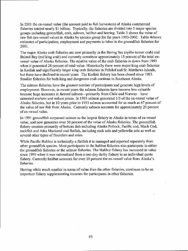
In 2001 the ex-vessel value (the amount paid to fish harvesters) of Alaska commercialfisheries totaled nearly $1 billion. Typically, the fisheries are divided into 5 major speciesgroups including groundfish, crab, salmon, halibut and herring. Table 3 shows the value ofraw fish (ex-vessel value) in Alaska by species group for the years 1993-2002. Table 4showsestimates of participation, employment and payments to labor in the groundfish fisheries for2001.
The major Alaska crab fisheries are now primarily in the Bering Sea (opilio tanner crab) andBristol Bay (red king crab) and currently constitute approximately 15 percent of the total ex-vessel value of Alaska fisheries. The relative value of the crab fisheries is down from 1993when it generated 28 percent of total value. Historically there were major king crab fisheriesin Kodiak and significantly larger king crab fisheries in Pribilof and St. Matthews Islands,but these have declined in recent years. The Kodiak fishery has been closed since 1983.Smaller fisheries for both king and dungeness crab continue in Southeast Alaska.
The salmon fisheries have the greatest number of participants and generate high levels ofemployment. However, in recent years the salmon fisheries have become less valuablebecause huge increases in farmed salmon-primarily from Chile and Norway-havesaturated markets and reduce prices. In 1993 salmon generated 1/3 of the ex-vessel value ofAlaska fisheries, but in 10 years prior to 1993 salmon accounted for as much as 67 percent ofthe value of raw fish from Alaska. Currently salmon accounts for approximately 20 percentof ex-vessel value.
In 1991 groundfish surpassed salmon as the largest fishery in Alaska in terms of ex-vesselvalue, and now generates over 50 percent of the value of Alaska fisheries. The groundfishfishery consists primarily of bottom fish including Alaska Pollock, Pacific cod, Black Cod,rockfish and Atka Mackerel and flatfish, including rock sole and yellowfin sole as well asseveral other types of flounders and soles.
While Pacific Halibut is technically a flatfish it is managed and reported separately fromother groundfish species. Most participants in the halibut fisheries also participate in eitherthe groundfish fisheries or the salmon fisheries. The Halibut fishery has increased in valuesince 1995 when it was rationalized from a one-day derby fishery to an individual quotafishery. Currently halibut accounts for over 10 percent the ex-vessel value from Alaska'sfisheries.
Herring while much smaller in terms of value than the other fisheries, continues to be animportant fishery supplementing incomes for participants in other fisheries.
93
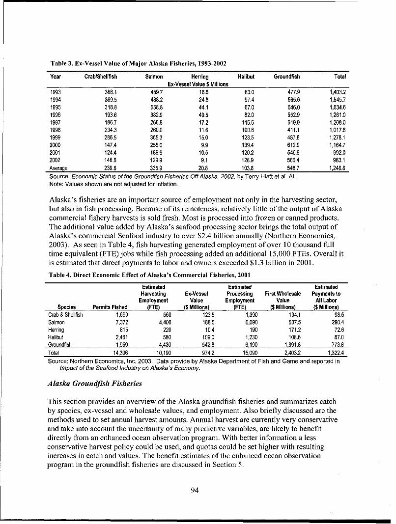
Table 3. Ex-Vessel Value of Major Alaska Fisheries, 1993-2002
Year CrablShellfish Salmon Herring Halibut Groundfish TotalEx-Vessel Value $ Millions
1993 386.1 459.7 16.6 63.0 477.9 1,403.21994 369.5 488.2 24.8 97.4 565.6 1,545.71995 318.8 558.8 44.1 67.0 646.0 1,634.61996 193.6 382.9 49.5 82.0 552.9 1,261.01997 186.7 268.8 17.2 115.5 619.9 1,208.01998 234.3 260.0 11.6 100.8 411.1 1,017.81999 286.5 365.3 15.0 123.5 487.8 1,278.12000 147.4 255.0 9.9 139.4 612.9 1,164.72001 124.4 189.9 10.5 120.2 546.9 992.02002 148.8 129.9 9.1 128.9 566.4 983.1Average 239.6 335.9 20.8 103.8 548.7 1,248.8Source: Economic Status of the Groundfish Fisheries Off Alaska, 2002, by Terry Hiatt et al. Al.Note: Values shown are not adjusted for inflation.
Alaska's fisheries are an important source of employment not only in the harvesting sector,but also in fish processing. Because of its remoteness, relatively little of the output of Alaskacommercial fishery harvests is sold fresh. Most is processed into frozen or canned products.The additional value added by Alaska's seafood processing sector brings the total output ofAlaska's commercial Seafood industry to over $2.4 billion annually (Northern Economics,2003). As seen in Table 4, fish harvesting generated employment of over 10 thousand fulltime equivalent (FTE) jobs while fish processing added an additional 15,000 FTEs. Overall itis estimated that direct payments to labor and owners exceeded $1.3 billion in 2001.
Table 4. Direct Economic Effect of Alaska's Commercial Fisheries, 2001
Estimated Estimated EstimatedHarvesting Ex-Vessel Processing First Wholesale Payments to
Employment Value Employment Value All LaborSpecies Permits Fished (FTE) ($ Millions) (FTE) ($ Millions) ($ Millions)
Crab & Shellfish 1,699 560 123.5 1,390 194.1 98.5Salmon 7,372 4,400 188.5 6,090 537.5 290.4Herring 815 220 10.4 190 171.2 72.6Halibut 2,461 580 109.0 1,230 108.6 87.0Groundfish 1,959 4,430 542.8 6,190 1,391.8 773.8Total 14,306 10,190 974.2 15,090 2,403.2 1,322.4Source: Northern Economics, Inc. 2003. Data provide by Alaska Department of Fish and Game and reported in
Impact of the Seafood Industry on Alaska's Economy.
Alaska Groundfish Fisheries
This section provides an overview of the Alaska groundfish fisheries and summarizes catchby species, ex-vessel and wholesale values, and employment. Also briefly discussed are themethods used to set annual harvest amounts. Annual harvest are currently very conservativeand take into account the uncertainty of many predictive variables, are likely to benefitdirectly from an enhanced ocean observation program. With better information a lessconservative harvest policy could be used, and quotas could be set higher with resultingincreases in catch and values. The benefit estimates of the enhanced ocean observationprogram in the groundfish fisheries are discussed in Section 5.
94
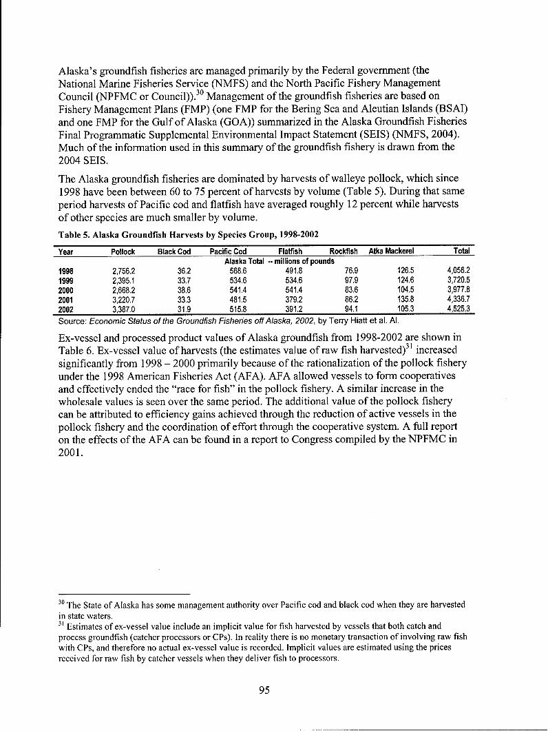
Alaska's groundfish fisheries are managed primarily by the Federal government (theNational Marine Fisheries Service (NMFS) and the North Pacific Fishery ManagementCouncil (NPFMC or Council)).3 ° Management of the groundfish fisheries are based onFishery Management Plans (FMP) (one FMP for the Bering Sea and Aleutian Islands (BSAI)and one FMP for the Gulf of Alaska (GOA)) summarized in the Alaska Groundfish FisheriesFinal Programmatic Supplemental Environmental Impact Statement (SEIS) (NMFS, 2004).Much of the information used in this summary of the groundfish fishery is drawn from the2004 SEIS.
The Alaska groundfish fisheries are dominated by harvests of walleye pollock, which since1998 have been between 60 to 75 percent of harvests by volume (Table 5). During that sameperiod harvests of Pacific cod and flatfish have averaged roughly 12 percent while harvestsof other species are much smaller by volume.
Table 5. Alaska Groundfish Harvests by Species Group, 1998-2002
Year Pollock Black Cod Pacific Cod Flatfish Rockfish Atka Mackerel TotalAlaska Total -- millions of pounds
1998 2,756.2 36.2 568.6 491.8 76.9 126.5 4,056.21999 2,395.1 33.7 534.6 534.6 97.9 124.6 3,720.52000 2,668.2 38.6 541.4 541.4 83.6 104.5 3,977.82001 3,220.7 33.3 481.5 379.2 86.2 135.8 4,336.72002 3,387.0 31.9 515.8 391.2 94.1 105.3 4,525.3
Source: Economic Status of the Groundfish Fisheries off Alaska, 2002, by Terry Hiatt et al. Al.
Ex-vessel and processed product values of Alaska groundfish from 1998-2002 are shown inTable 6. Ex-vessel value of harvests (the estimates value of raw fish harvested)3' increasedsignificantly from 1998 - 2000 primarily because of the rationalization of the pollock fisheryunder the 1998 American Fisheries Act (AFA). AFA allowed vessels to form cooperativesand effectively ended the "race for fish" in the pollock fishery. A similar increase in thewholesale values is seen over the same period. The additional value of the pollock fisherycan be attributed to efficiency gains achieved through the reduction of active vessels in thepollock fishery and the coordination of effort through the cooperative system. A full reporton the effects of the AFA can be found in a report to Congress compiled by the NPFMC in2001.
30 The State of Alaska has some management authority over Pacific cod and black cod when they are harvestedin state waters.3 1 Estimates of ex-vessel value include an implicit value for fish harvested by vessels that both catch and
process groundfish (catcher processors or CPs). In reality there is no monetary transaction of involving raw fishwith CPs, and therefore no actual ex-vessel value is recorded. Implicit values are estimated using the pricesreceived for raw fish by catcher vessels when they deliver fish to processors.
95
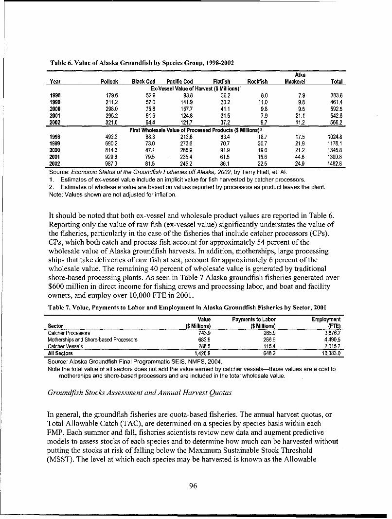
Table 6. Value of Alaska Groundfish by Species Group, 1998-2002
AtkaYear Pollock Black Cod Pacific Cod Flatfish Rockfish Mackerel Total
Ex-Vessel Value of Harvest ($ Millions) 1
1998 179.6 52.9 98.8 36.2 8.0 7.9 383.61999 211.2 57.0 141.9 30.2 11.0 9.8 461.42000 298.0 75.8 157.7 41.1 9.8 9.5 592.52001 295.2 61.9 124.8 31.5 7.9 21.1 542.62002 321.6 64.4 121.7 37.2 9.7 11.2 566.2
First Wholesale Value of Processed Products ($ Millions)21998 492.3 68.3 213.6 83.4 18.7 17.5 1024.81999 690.2 73.0 273.6 70.7 20.7 21.9 1178.12000 814.3 87.1 285.9 91.9 19.0 21.2 1345.82001 929.8 79.5 235.4 61.5 15.6 44.6 1390.82002 987.0 81.5 245.2 86.1 22.5 24.9 1482.8Source: Economic Status of the Groundfish Fisheries off Alaska, 2002, by Terry Hiatt, et. Al.1. Estimates of ex-vessel value include an implicit value for fish harvested by catcher processors.2. Estimates of wholesale value are based on values reported by processors as product leaves the plant.Note: Values shown are not adjusted for inflation.
It should be noted that both ex-vessel and wholesale product values are reported in Table 6.Reporting only the value of raw fish (ex-vessel value) significantly understates the value ofthe fisheries, particularly in the case of the fisheries that include catcher processors (CPs).CPs, which both catch and process fish account for approximately 54 percent of thewholesale value of Alaska groundfish harvests. In addition, motherships, large processingships that take deliveries of raw fish at sea, account for approximately 6 percent of thewholesale value. The remaining 40 percent of wholesale value is generated by traditionalshore-based processing plants. As seen in Table 7 Alaska groundfish fisheries generated over$600 million in direct income for fishing crews and processing labor, and boat and facilityowners, and employ over 10,000 FTE in 2001.
Table 7. Value, Payments to Labor and Employment in Alaska Groundfish Fisheries by Sector, 2001
Value Payments to Labor EmploymentSector ($ Millions) ($ Millions) (FTE)Catcher Processors 743.9 265.9 3,876.7Motherships and Shore-based Processors 682.9 266.9 4,490.5Catcher Vessels 288.5 115.4 2,015.7All Sectors 1,426.9 648.2 10,383.0Source: Alaska Groundfish Final Programmatic SEIS. NMFS, 2004.Note the total value of all sectors does not add the value earned by catcher vessels-those values are a cost to
motherships and shore-based processors and are included in the total wholesale value.
Groundfish Stocks Assessment and Annual Harvest Quotas
In general, the groundfish fisheries are quota-based fisheries. The annual harvest quotas, orTotal Allowable Catch (TAC), are determined on a species by species basis within eachFMP. Each summer and fall, fisheries scientists review new data and augment predictivemodels to assess stocks of each species and to determine how much can be harvested withoutputting the stocks at risk of falling below the Maximum Sustainable Stock Threshold(MSST). The level at which each species may be harvested is known as the Allowable
96
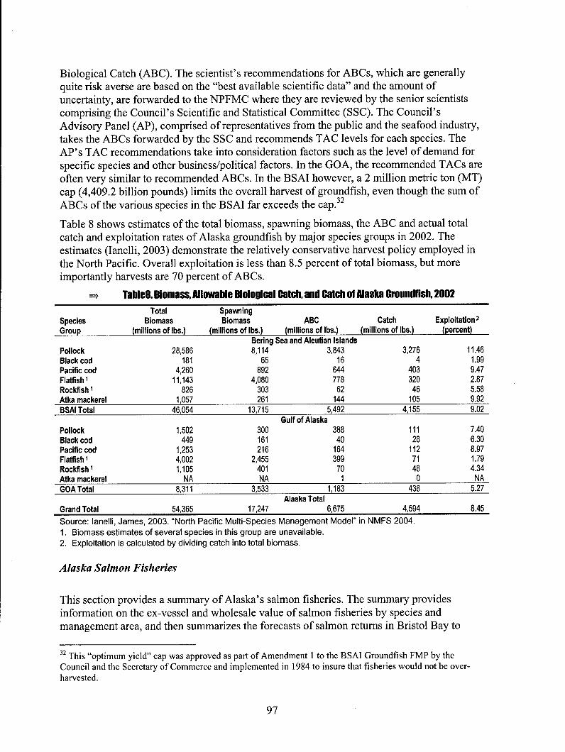
Biological Catch (ABC). The scientist's recommendations for ABCs, which are generallyquite risk averse are based on the "best available scientific data" and the amount ofuncertainty, are forwarded to the NPFMC where they are reviewed by the senior scientistscomprising the Council's Scientific and Statistical Committee (SSC). The Council'sAdvisory Panel (AP), comprised of representatives from the public and the seafood industry,takes the ABCs forwarded by the SSC and recommends TAC levels for each species. TheAP's TAC recommendations take into consideration factors such as the level of demand forspecific species and other business/political factors. In the GOA, the recommended TACs areoften very similar to recommended ABCs. In the BSAI however, a 2 million metric ton (MT)cap (4,409.2 billion pounds) limits the overall harvest of groundfish, even though the sum ofABCs of the various species in the BSAI far exceeds the cap.32
Table 8 shows estimates of the total biomass, spawning biomass, the ABC and actual totalcatch and exploitation rates of Alaska groundfish by major species groups in 2002. Theestimates (lanelli, 2003) demonstrate the relatively conservative harvest policy employed inthe North Pacific. Overall exploitation is less than 8.5 percent of total biomass, but moreimportantly harvests are 70 percent of ABCs.
=> Table8. Biomass, Allowable Biological Catch, and Catch of Alaska Groundfish, 2002
Total SpawningSpecies Biomass Biomass ABC Catch Exploitation 2
Group (millions of lbs.) (millions of lbs.) (millions of lbs.) (millions of lbs.) (percent)Bering Sea and Aleutian Islands
Pollock 28,586 8,114 3,843 3,276 11.46Black cod 181 65 16 4 1.99Pacific cod 4,260 892 644 403 9.47Flatfish 1 11,143 4,080 778 320 2.87Rockfish 1 826 303 62 46 5.58Atka mackerel 1,057 261 144 105 9.92BSAI Total 46,054 13,715 5,492 4,155 9.02
Gulf of AlaskaPollock 1,502 300 388 111 7.40Black cod 449 161 40 28 6.30Pacific cod 1,253 216 164 112 8.97Flatfish 1 4,002 2,455 399 71 1.79Rockfish 1 1,105 401 70 48 4.34Atka mackerel NA NA 1 0 NAGOA Total 8,311 3,533 1,183 438 5.27
Alaska TotalGrand Total 54,365 17,247 6,675 4,594 8.45
Source: lanelli, James, 2003. "North Pacific Multi-Species Management Model" in NMFS 2004.1. Biomass estimates of several species in this group are unavailable.
2. Exploitation is calculated by dividing catch into total biomass.
Alaska Salmon Fisheries
This section provides a summary of Alaska's salmon fisheries. The summary providesinformation on the ex-vessel and wholesale value of salmon fisheries by species andmanagement area, and then summarizes the forecasts of salmon returns in Bristol Bay to
32 This "optimum yield" cap was approved as part of Amendment I to the BSAI Groundfish FMP by the
Council and the Secretary of Commerce and implemented in 1984 to insure that fisheries would not be over-harvested.
97
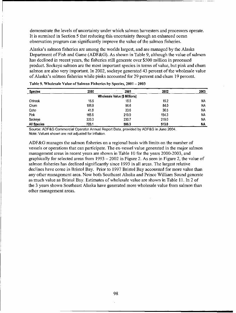
demonstrate the levels of uncertainty under which salmon harvesters and processors operate.It is surmised in Section 5 that reducing this uncertainty through an enhanced oceanobservation program can significantly improve the value of the salmon fisheries.
Alaska's salmon fisheries are among the worlds largest, and are managed by the AlaskaDepartment of Fish and Game (ADF&G). As shown in Table 9, although the value of salmonhas declined in recent years, the fisheries still generate over $500 million in processedproduct. Sockeye salmon are the most important species in terms of value, but pink and chumsalmon are also very important. In 2002, sockeye generated 43 percent of the wholesale valueof Alaska's salmon fisheries while pinks accounted for 29 percent and chum 19 percent.
Table 9. Wholesale Value of Salmon Fisheries by Species, 2001 - 2003
Species 2000 2001 2002 2003Wholesale Value ($ Millions)
Chinook 15.5 15.5 19.2 NAChum 166.9 96.6 84.0 NACoho 41.8 33.6 36.5 NAPink 165.6 219.9 154.3 NASockeye 333.3 230.7 219.0 NAAll Species 723.1 596.3 513.0 NASource: ADF&G Commercial Operator Annual Report Data, provided by ADF&G in June 2004.Note: Values shown are not adjusted for inflation.
ADF&G manages the salmon fisheries on a regional basis with limits on the number ofvessels or operations that can participate. The ex-vessel value generated in the major salmonmanagement areas in recent years are shown in Table 10 for the years 2000-2003, andgraphically for selected areas from 1993 - 2002 in Figure 2. As seen in Figure 2, the value ofsalmon fisheries has declined significantly since 1993 in all areas. The largest relativedeclines have come in Bristol Bay. Prior to 1997 Bristol Bay accounted for more value thanany other management area. Now both Southeast Alaska and Prince William Sound generateas much value as Bristol Bay. Estimates of wholesale value are shown in Table 11. In 2 ofthe 3 years shown Southeast Alaska have generated more wholesale value from salmon thanother management areas.
98
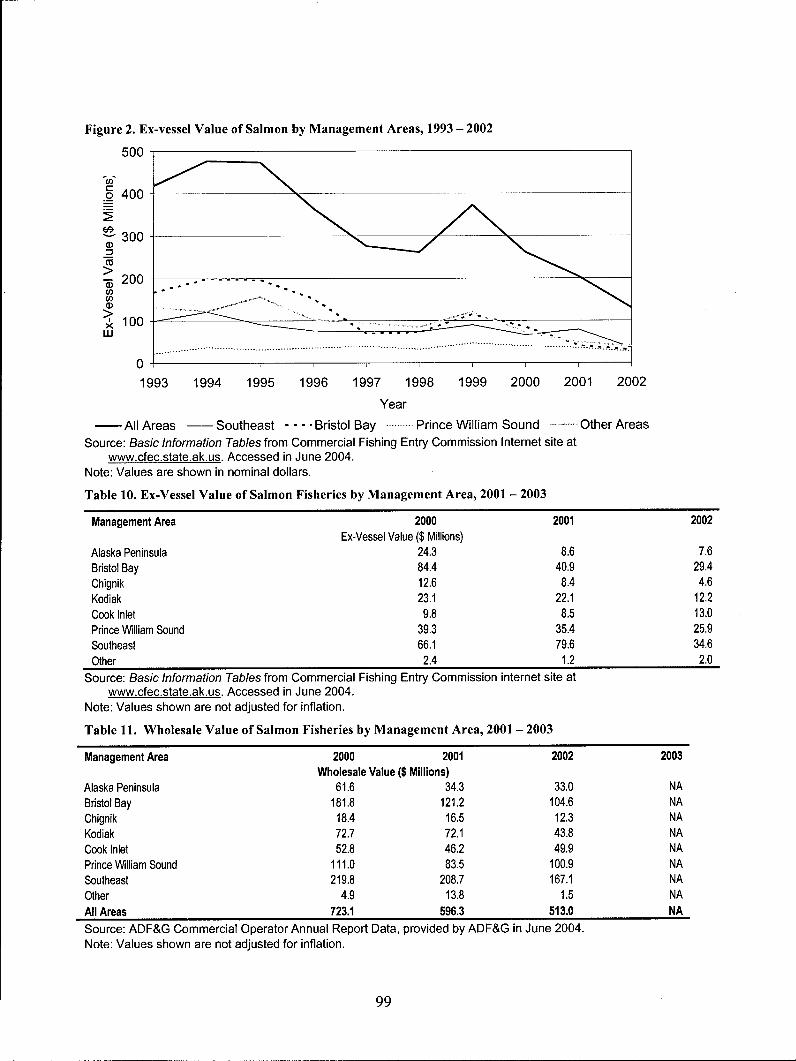
Figure 2. Ex-vessel Value of Salmon by Management Areas, 1993 - 2002
500
o 400
300
='3
-5 200 . ..
x 100
....................................................... . ."......... .....
1993 1994 1995 1996 1997 1998 1999 2000 2001 2002
Year
- AII Areas - Southeast --- Bristol Bay .......... Prince William Sound Other Areas
Source: Basic Information Tables from Commercial Fishing Entry Commission Internet site atwww.cfec.state.ak.us. Accessed in June 2004.
Note: Values are shown in nominal dollars.
Table 10. Ex-Vessel Value of Salmon Fisheries by Management Area, 2001 - 2003
Management Area 2000 2001 2002Ex-Vessel Value ($ Millions)
Alaska Peninsula 24.3 8.6 7.6Bristol Bay 84.4 40.9 29.4Chignik 12.6 8.4 4.6Kodiak 23.1 22.1 12.2Cook Inlet 9.8 8.5 13.0Prince William Sound 39.3 35.4 25.9Southeast 66.1 79.6 34.6Other 2.4 1.2 2.0
Source: Basic Information Tables from Commercial Fishing Entry Commission internet site atwww.cfec.state.ak.us. Accessed in June 2004.
Note: Values shown are not adjusted for inflation.
Table 11. Wholesale Value of Salmon Fisheries by Management Area, 2001 - 2003
Management Area 2000 2001 2002 2003Wholesale Value ($ Millions)
Alaska Peninsula 61.6 34.3 33.0 NABristol Bay 181.8 121.2 104.6 NAChignik 18.4 16.5 12.3 NAKodiak 72.7 72.1 43.8 NACook Inlet 52.8 46.2 49.9 NAPrince William Sound 111.0 83.5 100.9 NASoutheast 219.8 208.7 167.1 NAOther 4.9 13.8 1.5 NAAll Areas 723.1 596.3 513.0 NASource: ADF&G Commercial Operator Annual Report Data, provided by ADF&G in June 2004.Note: Values shown are not adjusted for inflation.
99
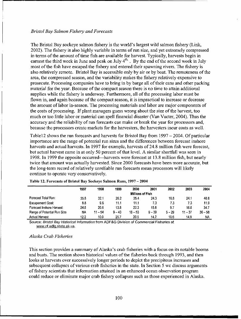
Bristol Bay Salmon Fishery and Forecasts
The Bristol Bay sockeye salmon fishery is the world's largest wild salmon fishery (Link,2002). The fishery is also highly variable in terms of run size, and yet extremely compressedin terms of the amount of time fish are available for harvest. Typically, harvests begin inearnest the third week in June and peak on July 4th . By the end of the second week in Julymost of the fish have escaped the fishery and entered their spawning rivers. The fishery isalso relatively remote. Bristol Bay is accessible only by air or by boat. The remoteness of thearea, the compressed season, and the variability makes the fishery relatively expensive toprosecute. Processing companies have to bring in by barge all of their cans and other packingmaterial for the year. Because of the compact season there is no time to attain additionalsupplies while the fishery is underway. Furthermore, all of the processing labor must beflown in, and again because of the compact season, it is impractical to increase or decreasethe amount of labor in-season. The processing materials and labor are major components ofthe costs of processing. If plant managers guess wrong about the size of the harvest, toomuch or too little labor or material can spell financial disaster (Van Vacter, 2004). Thus theaccuracy and the reliability of run forecasts can make or break the year for processors and,because the processors create markets for the harvesters, the harvesters incur costs as well.
Tablel 2 shows the run forecasts and harvests for Bristol Bay from 1997 - 2004. Of particularimportance are the range of potential run sizes and the differences between forecast inshoreharvests and actual harvests. In 1997 for example, harvests of 24.8 million fish were forecast,but actual harvest came in at only 50 percent of that level. A similar shortfall was seen in1998. In 1999 the opposite occurred-harvests were forecast at 13.8 million fish, but nearlytwice that amount was actually harvested. Since 2000 forecasts have been more accurate, butthe long-term record of relatively unreliable run forecasts mean processors will likelycontinue to operate very conservatively.
Table 12. Forecasts of Bristol Bay Sockeye Salmon Runs, 1997 - 2004
1997 1998 1999 2000 2001 2002 2003 2004Millions of Fish
Forecast Total Run: 35.8 32.1 26.2 35.4 24.3 16.8 24.1 46.6Escapement Goal: 8.8 9.6 11.1 11.1 7.3 7.3 7.3 11.9Forecast Inshore Harvest: 24.8 20.6 13.8 22.3 15.6 9.7 16.8 34.7Range of Potential Run Size NA 11-54 9-43 18-53 9-39 5-29 11-37 36- 58Actual Harvest 12.2 10.0 25.7 20.5 14.2 10.6 14.9 NASource: Bristol Bay Historical Information from ADF&G Division of Commercial Fisheries at
www.cf.adfiq.state.ak.us.
Alaska Crab Fisheries
This section provides a summary of Alaska's crab fisheries with a focus on its notable boomsand busts. The section shows historical values of the fisheries back through 1993, and thenlooks at harvests over successively longer periods to depict the precipitous increases andsubsequent collapses of various crab fisheries in the state. In Section 5 we discuss argumentsof fishery scientists that information attained in an enhanced ocean observation programcould reduce or eliminate major crab fishery collapses such as those experienced in Alaska.
100
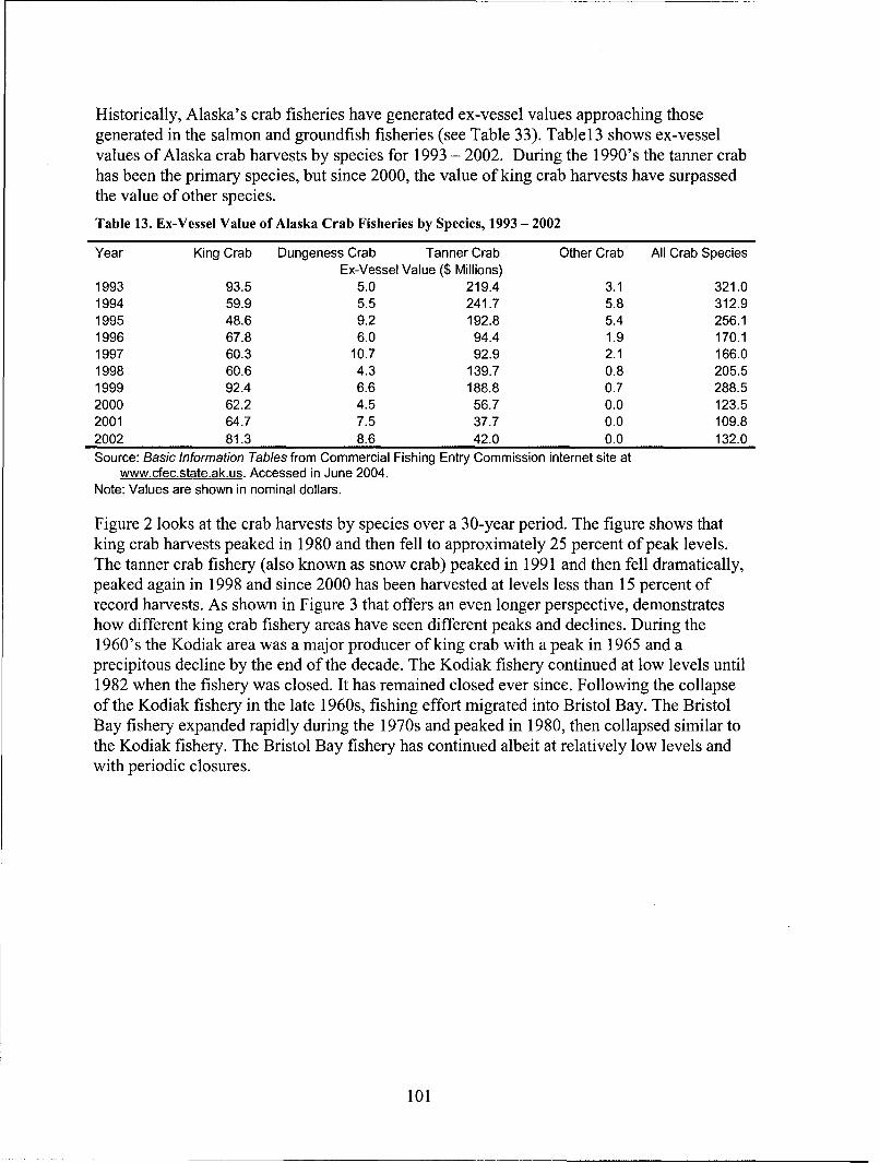
Historically, Alaska's crab fisheries have generated ex-vessel values approaching thosegenerated in the salmon and groundfish fisheries (see Table 33). Table 13 shows ex-vesselvalues of Alaska crab harvests by species for 1993 - 2002. During the 1990's the tanner crabhas been the primary species, but since 2000, the value of king crab harvests have surpassedthe value of other species.
Table 13. Ex-Vessel Value of Alaska Crab Fisheries by Species, 1993 - 2002
Year King Crab Dungeness Crab Tanner Crab Other Crab All Crab SpeciesEx-Vessel Value ($ Millions)
1993 93.5 5.0 219.4 3.1 321.01994 59.9 5.5 241.7 5.8 312.91995 48.6 9.2 192.8 5.4 256.11996 67.8 6.0 94.4 1.9 170.11997 60.3 10.7 92.9 2.1 166.01998 60.6 4.3 139.7 0.8 205.51999 92.4 6.6 188.8 0.7 288.52000 62.2 4.5 56.7 0.0 123.52001 64.7 7.5 37.7 0.0 109.82002 81.3 8.6 42.0 0.0 132.0Source: Basic Information Tables from Commercial Fishing Entry Commission internet site at
www.cfec.state.ak.us. Accessed in June 2004.Note: Values are shown in nominal dollars.
Figure 2 looks at the crab harvests by species over a 30-year period. The figure shows thatking crab harvests peaked in 1980 and then fell to approximately 25 percent of peak levels.The tanner crab fishery (also known as snow crab) peaked in 1991 and then fell dramatically,peaked again in 1998 and since 2000 has been harvested at levels less than 15 percent ofrecord harvests. As shown in Figure 3 that offers an even longer perspective, demonstrateshow different king crab fishery areas have seen different peaks and declines. During the1960's the Kodiak area was a major producer of king crab with a peak in 1965 and aprecipitous decline by the end of the decade. The Kodiak fishery continued at low levels until1982 when the fishery was closed. It has remained closed ever since. Following the collapseof the Kodiak fishery in the late 1960s, fishing effort migrated into Bristol Bay. The BristolBay fishery expanded rapidly during the 1970s and peaked in 1980, then collapsed similar tothe Kodiak fishery. The Bristol Bay fishery has continued albeit at relatively low levels andwith periodic closures.
101
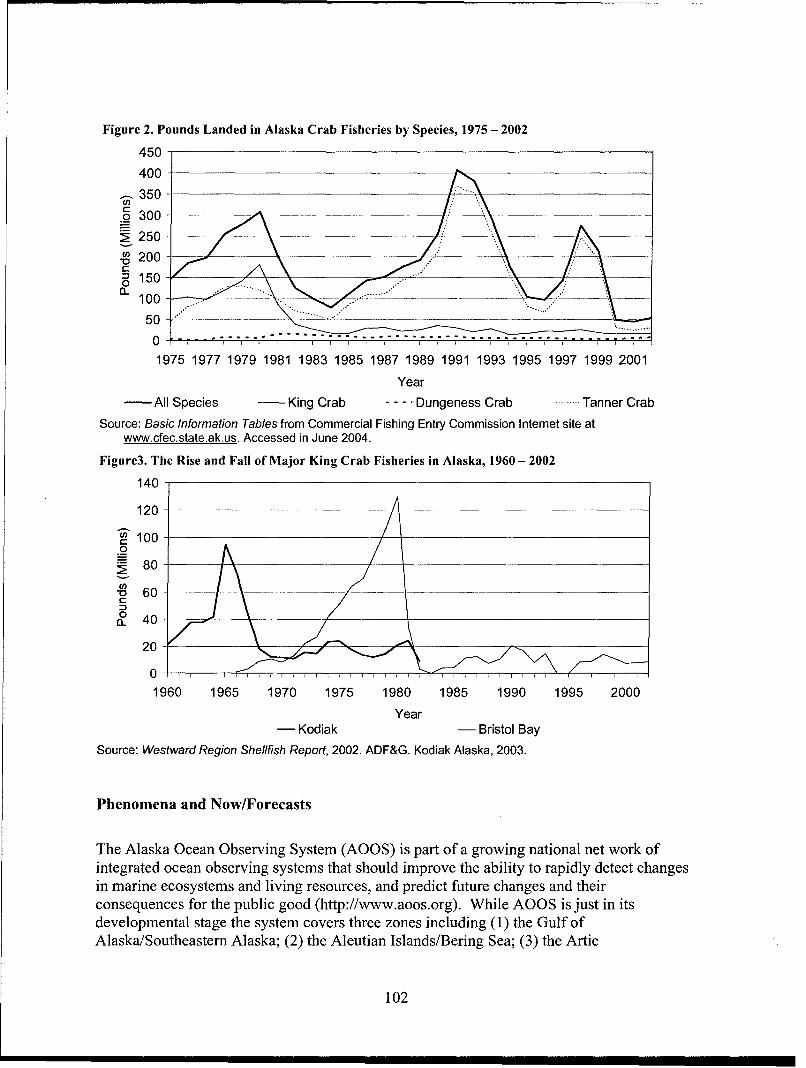
Figure 2. Pounds Landed in Alaska Crab Fisheries by Species, 1975 - 2002
450
400
350U,Co 300 - -- ---
S250
- 200
S1500
10050
1975 1977 1979 1981 1983 1985 1987 1989 1991 1993 1995 1997 1999 2001
Year- All Species - King Crab ---. Dungeness Crab .......... Tanner Crab
Source: Basic Information Tables from Commercial Fishing Entry Commission Internet site atwww.cfec.state.ak.us. Accessed in June 2004.
Figure3. The Rise and Fall of Major King Crab Fisheries in Alaska, 1960 - 2002
140
120
100
80
U)-66
0o~40
20
01
1960 1965 1970 1975 1980 1985 1990 1995 2000
Year- Kodiak - Bristol Bay
Source: Westward Region Shellfish Report, 2002. ADF&G. Kodiak Alaska, 2003.
Phenomena and Now/Forecasts
The Alaska Ocean Observing System (AOOS) is part of a growing national net work ofintegrated ocean observing systems that should improve the ability to rapidly detect changesin marine ecosystems and living resources, and predict future changes and their
consequences for the public good (http://www.aoos.org). While AOOS is just in itsdevelopmental stage the system covers three zones including (1) the Gulf ofAlaska/Southeastern Alaska; (2) the Aleutian Islands/Bering Sea; (3) the Artic
102
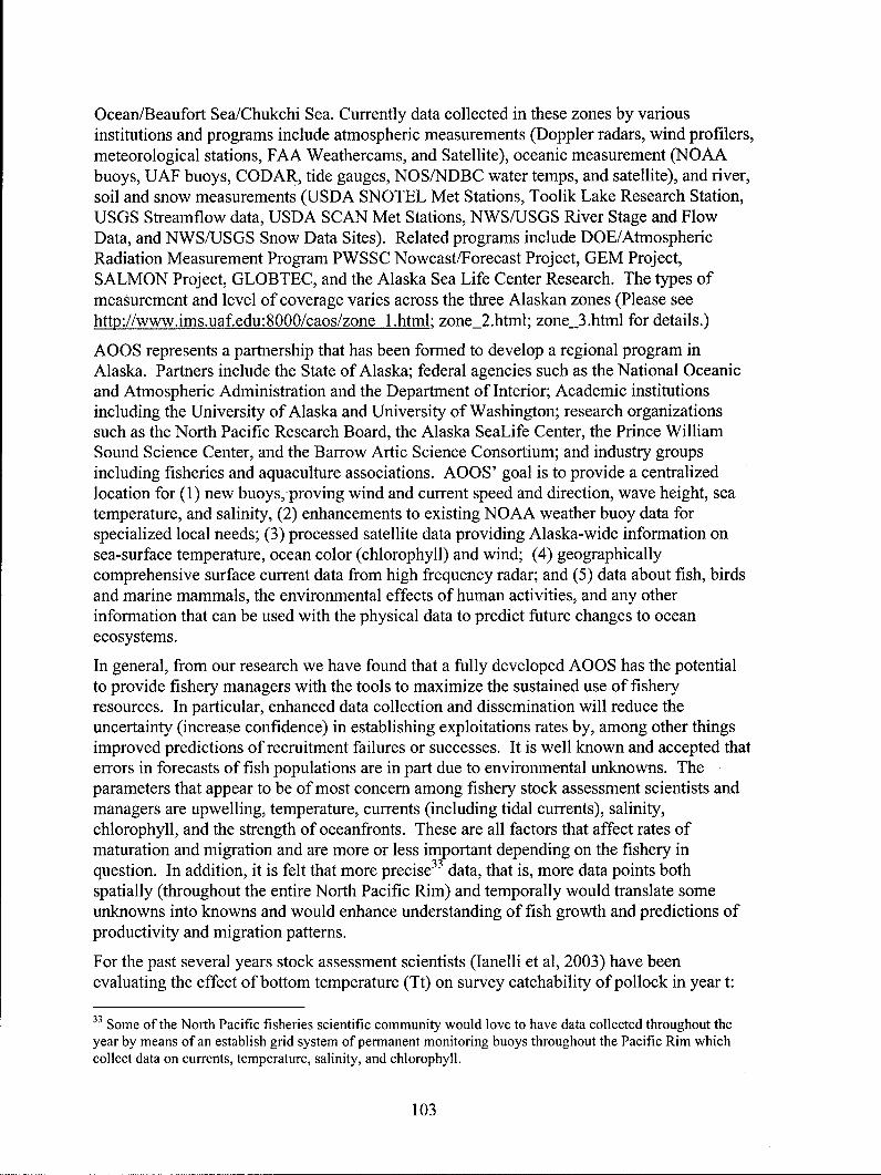
Ocean/Beaufort Sea/Chukchi Sea. Currently data collected in these zones by variousinstitutions and programs include atmospheric measurements (Doppler radars, wind profilers,meteorological stations, FAA Weathercams, and Satellite), oceanic measurement (NOAAbuoys, UAF buoys, CODAR, tide gauges, NOS/NDBC water temps, and satellite), and river,soil and snow measurements (USDA SNOTEL Met Stations, Toolik Lake Research Station,USGS Streamflow data, USDA SCAN Met Stations, NWS/USGS River Stage and FlowData, and NWS/USGS Snow Data Sites). Related programs include DOE/AtmosphericRadiation Measurement Program PWSSC Nowcast/Forecast Project, GEM Project,SALMON Project, GLOBTEC, and the Alaska Sea Life Center Research. The types ofmeasurement and level of coverage varies across the three Alaskan zones (Please seehttp://www.ims.uaf.edu:8000/caos/zone 1.html; zone_2.html; zone_3.html for details.)
AOOS represents a partnership that has been formed to develop a regional program inAlaska. Partners include the State of Alaska; federal agencies such as the National Oceanicand Atmospheric Administration and the Department of Interior; Academic institutionsincluding the University of Alaska and University of Washington; research organizationssuch as the North Pacific Research Board, the Alaska SeaLife Center, the Prince WilliamSound Science Center, and the Barrow Artic Science Consortium; and industry groupsincluding fisheries and aquaculture associations. AOOS' goal is to provide a centralizedlocation for (1) new buoys,-proving wind and current speed and direction, wave height, seatemperature, and salinity, (2) enhancements to existing NOAA weather buoy data forspecialized local needs; (3) processed satellite data providing Alaska-wide information onsea-surface temperature, ocean color (chlorophyll) and wind; (4) geographicallycomprehensive surface current data from high frequency radar; and (5) data about fish, birdsand marine mammals, the environmental effects of human activities, and any otherinformation that can be used with the physical data to predict future changes to oceanecosystems.
In general, from our research we have found that a fully developed AOOS has the potentialto provide fishery managers with the tools to maximize the sustained use of fisheryresources. In particular, enhanced data collection and dissemination will reduce theuncertainty (increase confidence) in establishing exploitations rates by, among other thingsimproved predictions of recruitment failures or successes. It is well known and accepted thaterrors in forecasts of fish populations are in part due to environmental unknowns. Theparameters that appear to be of most concern among fishery stock assessment scientists andmanagers are upwelling, temperature, currents (including tidal currents), salinity,chlorophyll, and the strength of oceanfronts. These are all factors that affect rates ofmaturation and migration and are more or less important depending on the fishery inquestion. In addition, it is felt that more precise 33 data, that is, more data points bothspatially (throughout the entire North Pacific Rim) and temporally would translate someunknowns into knowns and would enhance understanding of fish growth and predictions ofproductivity and migration patterns.
For the past several years stock assessment scientists (lanelli et al, 2003) have beenevaluating the effect of bottom temperature (Tt) on survey catchability of pollock in year t:
33 Some of the North Pacific fisheries scientific community would love to have data collected throughout theyear by means of an establish grid system of permanent monitoring buoys throughout the Pacific Rim whichcollect data on currents, temperature, salinity, and chlorophyll.
103
Q(t)= U(q) +BqTt
Where Uq is the mean catchability and Bq represents the slope parameter. Bottomtemperature was collected during the NMFS summer bottom-trawl surveys. It was shownthat temperature affects the distribution of pollock on the shelf and by extension could affectthe availability of the stock to survey. That is, temperature may affect the proportion of thestock that is within or outside of the standard survey area. These patterns were furtherexamined by comparing Pollock density with selected on-bottom isotherms. This shows that2002 was warmer than usual and that, in general, pollock densities are rare at temperatureslower than 0 degrees. The latter illustrates the significant value of the understanding of theeffect of this physical parameter on the evaluation and determination of allowable biologicalcatch in fisheries management.
Another growing body of scientific evidence supports hypotheses about the direct andindirect effects of the environmental change on salmon production (NPAFC Science Plan2001-2005, BASIS). For example there is a strong correspondence between salmon catchand climate indices. In addition, there appears to be a correlation between water temperature,blooms of coccolithophorid and salmon survival (Jack Helle, Alaska Fisheries ScienceCenter, Auk Bay Lab May, 2004). Over the last 6 years there have been two significantlong-term blooms in the Bering Sea (the blooms being an indication of sterile oceanconditions). According to Helle, coccolithophorid blooms appear to be water temperaturerelated. If the scientists have better forecasts on water temperature they could better predictthe occurrence of these blooms and thus be better able to predict juvenile salmon survival.
It is also hypothesized by Alaska Department of Fish and Game that physical oceanographicdata can improve management of Cook Inlet sockeye salmon through improvements inseason salmon run projections (Willette and Pegau, 2002). In 1999, the Alaska Board ofFisheries adopted a sliding range of inriver escapement goals for late-run Kenai RiverSockeye salmon that were based upon preseason and inseason projections of the annualreturn of this salmon stock. The ADF&G offshore test fishing (OTF) provides the primarysource of information used to project the return of this stock inseason. Achievement ofinriver escapement goals and allocation of salmon to commercial, personal use andrecreational user groups is thus largely dependent on the accuracy of these projections. Theaccuracy of the population estimates provided by OTF typically increases as the seasonprocesses. Projections made on July 20 have ranged from -5.4% to +103% of the actual run.Errors in OTF program estimates or run size appear to be due to interannual changes inmigratory timing and catchability.
The OTF program often fails to accurately predict runs that are earlier than normal. Failureto accurately predict very large runs can result in large escapements, loss of revenue to thecommercial fishery, and reduced production in future years due to overgrazing of planktonstocks by large fry populations in rearing lakes. Failure to accurately predict weak runs canresult in over harvest by the commercial fishery and reduced production in future years.Errors in OTF program estimates of run size appear to be due to interannual changes inmigratory timing and catchability. Migratory timing is defined as abundance as a function oftime in a fixed geographic reference frame (Mundy, 1982). The sockeye run entering theCook Inlet normally peaks on July 15, but peak migratory timing has varied from Jul6 to July19. According to Willette and Pegau, variations in migratory timing are likely due to a rangeof biotic and physical factors that affect rates of maturations and migrations. Ocean
104
temperature (Burgner, 1980), the strength of oceanic fronts (Mundy, 1982), and tidal currents(Stasko et al., 1973) are all likely important physical factors affecting both the rate ofmaturation and migration of salmon. Catchability is defined as the fraction of the populationcaptured by a unit of fishing gear. The OTF program estimates cumulative catchability todate from the ratio of cumulative catch per unit of effort (CPUE) obtained from the testfishing vessel and estimates of total return to date. Cumulative catchability varies by a factorof 2 among years. Variations in catchability are likely due to biotic factors (e.g. fish size) aswell as physical factors that affect the vertical and horizontal distribution and migration rateof salmon (Hakoyama, 1995).
The migration of salmon into the Cook Inlet is clearly influenced by the strength and locationof tiderips. Fishermen working the inlet are very aware of the tiderips and use the rips tolocate and capture migrating salmon (Wilson and Tomlins, 1999). Salmon have likelyevolved behaviors that allow them to use rip tides and associated current structures tominimize the energy expended to reach their natal rivers (Scholz et al. 1972). According toWillette and Pegau, (2004) although tiderips clearly result from strong velocity gradients,they also represent boundaries between water masses and may be associated with strongsalinity gradients.
Willette and Pegau have proposed to test several hypotheses regarding the effects ofchanging oceanographic conditions on the migratory behavior and catchability of salmonentering Cook Inlet. Better understanding of these effects may allow for improvement in theaccuracy of inseason sockeye salmon populations estimates and thus improved accuracy ofshort and long-term forecasts of salmon runs. The latter suggests that with ongoingoceanographic data collection through AOOS ADF&G might be able to better manage forinriver escapement goals and maximize sustained yield thus benefiting the economy of theUpper Cook Inlet area and nation as a whole.
Currently, OOS information is not readily used in the crab industry. Sometimes fisheriesmanagers use weather data to adjust fishing seasons (for safety reasons). In addition, bottomtemperature information is sometimes used as an indicator of species distribution andcorrelated over time to stock size. However, in general, according to our sources, thegreatest benefit to the Alaskan king and tanner crab industry from enhanced AOOS would bein the long term with the collection of appropriate time series data. Biological andoceanographic data could be correlated with trawl surveys and allow fisheries biologists tobetter predict crab recruitment and productivity. This information could be used to developharvest rate models that more adequately reflect the state of the ecosystem. According toGordon Kruse (ADF&G) oceanographic conditions (upwelling, temperature and currents) arecritical to the development of larvae for nearly all species of crab. For example, egg andlarvae development are temperature sensitive. Larvae feed on phytoplanktons that are lightsensitive. If winter/spring is cold then it is likely that phytoplankton blooms will occurbefore the crab larvae are developmentally ready. Better oceanographic data would allowfisheries scientists and fisheries managers to better predict poor and good recruitment andthus allow for more accurate determinations about when to close and or open a fishery.
In addition to the above, we have learned that the value of AOOS will probably be highest inthe rationalized fisheries. The fleet may benefit from more detailed knowledge of thedistribution of fish by age and season. This would allow them to minimize unintended catchof non-targeted species (an unintended consequence but of significant value to society)
105
minimizing fuel and crew costs. For example, if scientists knew enough to state that duringthe summer months, adult pollock will follow a particular frontal feature and can identifywhere that front is located they could provide the fleet with forecasts of prime fishinglocations for target species.
Finally, we have learned that there are also benefits or value from enhanced data collectionand dissemination through AOOS to fisheries managers as relates to Essential Fish HabitatProvisions, Marine Protected Areas and marine mammal protection. Fisheries managersneed and want better data to allow them to now deal with the complex spatial and temporaldimensions associated with ecosystem-based management tools that are the underpinnings ofthe above management tools.
One scenario that we have not explored but for which potential economic benefits ofenhanced OOS may be accrued is the shellfish aquaculture industry and human health andsafety more generally. If, for example, scientists could more accurately predict blooms ofPSP (paralytic shellfish poisoning) industry would know to terminate production activitiesand thus avoid significant health and safety consequences. PSP is a fairly significant issue inthe Washington aquaculture industry and better information about the timing and extent ofalgal blooms could have measurable economic benefits in the near future as opposed to therelatively more speculative and long term future benefits of better recruitment forecasts andstock assessments as described above.
Qualitative Discussion of Fishery Management Decision Making
Prediction of fish stocks or population levels plays a critical role in fisheries managementdecision-making. Prediction of stock size is critical to the underlying principals or goals ofsustainable fisheries management. As such the role of fishery scientists is great in the overalldecisions about harvest strategies. However, there continues to be tremendous uncertainty instock size projections and thus continued potential for less than perfect decision making atthe management level. Authors such as Solow et al (1998) have been able to use data onenhanced forecasts of oceanographic conditions to formulate predictions of crop yields whichare then used by farmers to optimize cropping patterns. The Bayesian decision theoryapproach that they use could potentially provide a methodology to aid fisheries managers inoptimizing fish harvest (given the constraints of provisions of the MSFMCA and otherpertinent legislation and regulation and fishery management objectives through the tenNational Standards for Fishery Conservation and Management). The Bayesian approachcould be used as a management tool to make predictions and explore the consequences ofalternative scenarios for a particular fishery within a particular ecosystem. The aim of thisapproach would be to develop a model as a tool for guiding decision making in a variety ofareas including the conduct of a fishery, and the targeted collection of information toimprove understanding of the system and its response to change (Goodman et al, 2002).
That said it is instructive to qualitatively outline the decision model that is used in fisheriesmanagement decision-making in the Alaska region. Goodman et al (2002 pp. 1-2) provides anexcellent guide for lay persons of the very complex process by which harvest strategies arechosen. The following is taken from that report which explicitly focuses on Alaskagroundfish species management.
106
The current harvest decision making strategy is essentially a maximum sustainable yield(MSY) single-species approach, modified by some formal safeguards incorporated to wardagainst overfishing as defined from the single-species stand point, and with opportunities of aless-structured nature for reducing harvest rates further in response to perceived social,economic and ecological concerns. No quantitative standards or specific decision rules arestated for these latter considerations, except as they are imposed, from outside the MSFCMA,by the Endangered Species Act or the Marine Mammal Protection Act.
The overfishing level (OFL) set for each stock is an estimate either of the fishing mortalityrates associated with MSY (Fmsy) or an estimate of a surrogate for Fmsy. The OFL istreated in the management system as a limit that should not be exceeded except with a verylow probability. The acceptable biological catch (ABC) set for each stock is an estimate of atarget rate, which is intended to establish some margin between it and the OFL. The hope isthat managing so as to achieve this target on average will accomplish the desired compliancewith exceeding the limit (OFL) only rarely. The ad hoc downward adjustments of harvest inresponse to other social, economic, and ecological considerations takes place in thedeliberations where the total allowable catch (TAC) is set subject to the constraint that it beless than or equal to the ABC.
The formulaic component of the reduction of harvest rate from the theoretical MSY harvestrate (from OFL to ABC) is by an amount that is often modest, when expressed as a fractionof the harvest rate; but in terms of the total tonnage involved, or its dollar value, the amountis considerable. The margin is also small relative to real natural variation, and small relativeto the practical uncertainty about stock status or population parameters for many of the targetstocks and indeed for most of the ecosystem. By contrast, in actual practice, the reduction inTAC from ABC has for some stocks and some years been quite large, but there is no explicitand general formula for this reduction. Many stock assessment scientists believe that thisbuffer should be better linked to uncertainty in both the measurement and process error(Anne Hollowed, personal conversation 2004).
The formal and standardized quantitative portions of the process for determining OFL andABC begin with the assignment of each stock to one of six "Tiers" based on the availabilityof information about that stock. Tier 1 has the most information, and Tier 6 the least. Theso-called F40% construct plays a prominent role in some of the Tiers but not others. F40% isthe calculated fishing mortality rate at which equilibrium spawning biomass per recruit isreduced to 40% of its value in the equivalent unfished stock. This is an esoteric, but useful,measure of the amount by which the associated fishing rate reduced the stock size, in thelong run. The useful features of this particular measure are two-fold. First, its calculation isless sensitive to the details of the stock-recruitment relationship than is the calculation ofFmsy, so it is practical to estimate F40% for stocks that are not well enough studied forestimation of Fmsy. The second is that for a range of dynamics encompassing many, but notall, of the BSAI/GOA target groundfish stocks, for example, modeling studies have shownthat harvesting at F35% accomplishes about the same thing as harvesting at Fmsy, soharvesting at the slightly lower rate, F40% established a modest margin of safety.
Currently management of king and Tanner crab fisheries are under the jurisdiction of theAlaska Department of Fish and Wildlife and National Marine Fisheries Service. An annualstock assessment and fishery evaluation (SAFE) report is required of them by the NorthPacific Fisheries Management Council. The SAFE summarizes among other things,
107
guideline harvest levels (GHL) and analytical information used for management decisions orchanges in harvest strategies. According to the 2003 SAFE for King and Tanner CrabFisheries sin the Bearing Sea and Aleutian Islands, the Federal requirements for determiningthe status of the stocks are the minimum stock size threshold (MSST) and the maximumfishing mortality threshold (MFMT). These requirements are contained in the FisheriesManagement Plan (FMP). The MSST is 50% of the man total spawning biomass (SB orTMB= total mature biomass) for the period 1983-1997, upon which the maximumsustainable yield (MSY) was based. A stock is overfished if the SB is below the MSST. TheMFMT is represented by the sustainable yield (SY) in a given year, which is the MSY ruleapplied to the current SB (the MSY control rule is F=0.2 for king crabs and F=0.3 for Tannerand snow crabs). Overfishing occurs if the harvest level exceeds the SY in one year. GHLsare developed from joint NMFS and ADF&G assessment of stock conditions based onharvest strategies developed by ADF&G.
Regular trawl and hydoraccoustic survey results for five stocks (Pribilof blue king crab, St.Matthew blue king crab, Bristol Bay red king crab, eastern Bering Sea Tanner crab (c.bairdi), and eastern Bering Sea snow crab (c. opilio) are compared to thresholds establishedby the State of Alaska harvest strategies and regulations. ADF&G uses these thresholds todetermine if a fishery should be opened and to calculate GHL. For example, the Bering SeaTanner crab fishery was closed in 1997 due to near record low stock abundance in the 1997NMFS survey and poor performance in the 1996 fishery. ADF&G will reopen the fisherywhen the female biomass is above the threshold and the fishery GHL is above the minimumidentified in the rebuilding harvest strategy or MSY biomass defined in the FMP as 189.6million pounds of total mature biomass.
The traditional approach to fishery science, that is, the primary input to the harvest strategyoutlined above, has been to assess the state of the stocks on a single-species basis, usingcatch and biological data as input to the models and then forecast what will happen if things(usually total catches) stay as they are or get changed somewhat. This leads to decisionsbeing made based on expected outcomes. Some sense of the robustness of decisions can bemade by running the forecasts with different assumptions or from different starting points butthis sort of exploration has traditionally been limited and ad hoc. A more recent approach isinstead to create models of the fishery systems and to use computer simulations to testsystematically what would happen if different management strategies (combinations of datacollection, assessment and decisions following specific rules) were adopted. This sort ofanalysis is aimed at systematically revealing how different management approaches comparein meeting sets of objectives. Unfortunately given the scope of this work we are not able toexplore and implement this approach at this time. In general, however, we have been able toascertain that enhanced AOOS offers the potential greatest benefits at the scientific levelwhere science can monitor, assesses forecasts within bounds and generally inform andsupport decision making. At this point stock assessment scientists feel limited in theircapabilities and feel that more atmospheric, oceanic, biological and ecosystem data would beof tremendous benefit. Once such data is made more available they feel several years ofimproved predictions (better than correct 60% of the time) will be required in order to gainthe trust of fisheries managers and the fishing community and ultimately have theirrecommendations for such metrics as total allowable catch (TAC) to be readily accepted.
108
Assessment of the Economic Value of an Enhanced Ocean Observation Program
An enhanced ocean observation program has the potential to provide significant benefits toAlaska commercial fisheries. This section discusses three areas where better information andless uncertainty could generate higher values:
1) Better information could improve the reliability of forecasts that in turn will enhancethe ability of fishery businesses to plan their fishing seasons and profitably prosecutetheir fisheries. In Alaska salmon fisheries it is estimated that reducing the uncertaintydue to unreliable run size and timing forecasts, would lead to increases in netrevenues for salmon processors by $77 million per year
2) Better information and more certainty could allow a more aggressive harvest policy inthe Alaska groundfish fisheries without placing stocks under undue risk ofoverfishing. Improvements due to better information could generate an estimated$504 million in additional wholesale value per year.
3) Better information and more certainty could allow a more aggressive harvest policy inthe Alaska groundfish fisheries without placing stocks under undue risk ofoverfishing. Improvements due to better information could generate an estimated$504 million in additional wholesale value per year.
Enhanced Business Planning - Alaska Salmon Fisheries
Analysts at Northern Economics interviewed key informants at three of the top five Alaskasalmon processors-Don Giles at Icicle Seafoods, Terry Gardiner at Norquest, and NormVan Vacter at Peter Pan Seafoods. Processors were asked to describe how improved certaintyin run forecasts would help their operations with particular reference to Bristol Bay. All threeagreed separately, that if an enhanced ocean observation system could significantly improverun size and timing forecasts, then the benefits to their bottom lines would be verysignificant. In general it was felt that improvement in profits from Bristol Bay could rangefrom $25 to $50 million per year.
Improvements would come in three areas: 1) from cost savings and efficiency gains, 2) fromincreased processing amounts when forecast runs are high, and 3) from higher wholesaleprices on average.
Cost savings and efficiency gains would be generated if processors could rely on run size andrun timing forecasts, and if the range of the forecasts was smaller. The savings would berealized in the amount of processing materials and labor that are deployed to the facility.With greater certainty the amount of material and labor can be optimized.
With high levels of uncertainty processors tend to be conservative in their planning. In yearswith high run size forecasts most processors will plan on harvests in the low end of theforecast range. The costs of underestimating labor and material needs are lower than the costsof overestimating. Once the material and labor is acquired and deployed they become sunkcosts, and if the runs fail to materialize then operating losses are likely. Thus if there isgreater certainty and reliability in the forecasts, processors will learn to be more aggressive in
109
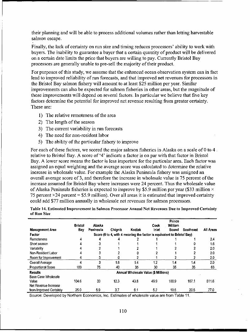
their planning and will be able to process additional volumes rather than letting harvestablesalmon escape.
Finally, the lack of certainty on run size and timing reduces processors' ability to work withbuyers. The inability to guarantee a buyer that a certain quantity of product will be deliveredon a certain date limits the price that buyers are willing to pay. Currently Bristol Bayprocessors are generally unable to pre-sell the majority of their product.
For purposes of this study, we assume that the enhanced ocean observation system can in factlead to improved reliability of run forecasts, and that improved net revenues for processors inthe Bristol Bay salmon fishery will amount to at least $25 million per year. Similarimprovements can also be expected for salmon fisheries in other areas, but the magnitude ofthose improvements will depend on several factors. In particular we believe that five keyfactors determine the potential for improved net revenue resulting from greater certainty.These are:
1) The relative remoteness of the area2) The length of the season3) The current variability in run forecasts4) The need for non-resident labor5) The ability of the particular fishery to improve
For each of these factors, we scored the major salmon fisheries in Alaska on a scale of 0 to 4relative to Bristol Bay. A score of '4' indicate a factor is on par with that factor in BristolBay. A lower score means the factor is less important for the particular area. Each factor wasassigned an equal weighting and the average score was calculated to determine the relativeincrease in wholesale value. For example the Alaska Peninsula fishery was assigned anoverall average score of 3, and therefore the increase in wholesale value is 75 percent of theincrease assumed for Bristol Bay where increases were 24 percent. Thus the wholesale valueof Alaska Peninsula fisheries is expected to improve by $5.9 million per year ($33 million x75 percent x24 percent = $5.9 million). Over all areas it is estimated that improved certaintycould add $77 million annually in wholesale net revenues for salmon processors.
Table 14. Estimated Improvement in Salmon Processor Annual Net Revenues Due to Improved Certaintyof Run Size
PrinceBristol Alaska Cook William
Management Area Bay Peninsula Chignik Kodiak Inlet Sound Southeast All AreasFactor Score (0 to 4, with 4 meaning the factor is equivalent to Bristol Bay)Remoteness 4 4 4 2 1 1 1 2.4Short season 4 3 1 1 1 1 0 1.6Variability 4 2 1 2 1 2 2 2.0Non-Resident Labor 4 3 2 0 2 1 2 2.0Room for Improvement 4 3 0 2 1 2 2 2.0Overall Average 4 3 1.6 1.4 1.2 1.4 1.4 2.0Proportional Score 100 75 40 35 30 35 35 63Results Annual Wholesale Value ($ Millions)Base Case WholesaleValue 104.6 33 12.3 43.8 49.9 100.9 167.1 511.6Net Revenue Increasefrom Improved Certainty 25.0 5.9 3.7 6.1 5.2 10.6 20.5 77.0Source: Developed by Northern Economics, Inc. Estimates of wholesale value are from Table 11.
110
These benefits are measures of producer surplus as most of the improvement would be aresult of reduced costs to harvesters and producers. There might also be some improvementin product quality as fish are harvested earlier in the season and a shift to fillets (with greatervalue added) from headed and gutted (lower value added) also leading to improvements inboth producer and consumer surplus. Finally, because of increased product quality andgreater value added, total processed product output ( 1 st wholesale value) from the regionwould increase resulting also in increased regional economic impacts.
Increased Harvests - Alaska Groundfish Fisheries
As indicated in Section 2, stock assessments and harvest quotas for groundfish take intoaccount the amount of uncertainty in each of the utilized species. Scientists recommendrelatively low ABCs for species with high levels of uncertainty in key variables, but willrecommend relatively high ABCs for species where there is more certainty. It is suggested(Anne Hollowed, NMFS/REFM) that use of temperature data can be used to reduce stocksize forecast error. Currently NMFS is correct only 60% of the time in their annual pollockstock assessment. The risk adverse nature of groundfish harvest strategies is furthered by anabsolute limit on TACs in the Bering Sea of 2 million metric tons. Without this "OY Cap"harvests in the Bering Sea could significantly increase.
For purposes of this study fishery scientists from NOAA's Alaska Fishery Science Centerwere asked what harvests levels of groundfish might look like if enhancements to AOOS ledto significant improvements in their ability to accurately predict (on a relative scale) stocksizes and recruitment of major groundfish species. Scientists indicated that constraintsimposed within their stock assessment models to account for uncertainty could be reducedand that recommended ABCs would increase significantly for many of the groundfishspecies. Furthermore if there was a longer track record of improved stock assessments it issurmised that political decisions to limit overall harvests would eventually be removed andthat TACs would approach recommended ABCs.
While not developed specifically for this study the "North Pacific Multi-SpeciesManagement Model" developed by Dr. James Janelli includes an assessment of groundfishharvests under the assumption that uncertainty in stock levels and recruitment are greatlyreduced, and that artificial caps on harvests are eliminated. The model was originallydeveloped for use in the Alaska Groundfish Fisheries Final Programmatic SupplementalEnvironmental Impact Statement (NMFS 2004) and the assessment of harvests with theassumption of high levels of certainty corresponds to Alternative 2.1 in the SEIS. The modelresults for the base case and the case with improved information are shown in Table 15. Theresults demonstrate the possibility that with improved information catch and value in thefisheries can be improved significantly. The long run average increase in wholesale valueprojecting out 20 years from the base year (2002) is over $500 million annually. Whileprojections of overall biomass are expected to decline, constraints in the model assures thatexploitation rates do not cause stocks to fall below sustainable levels.
111
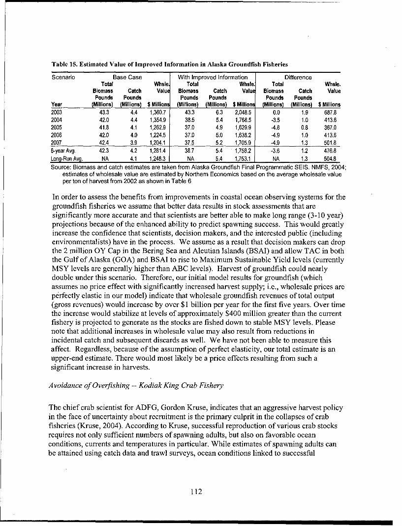
Table 15. Estimated Value of Improved Information in Alaska Groundfish Fisheries
Scenario Base Case With Improved Information DifferenceTotal Whsle. Total Whsle. Total Whsle.
Biomass Catch Value Biomass Catch Value Biomass Catch ValuePounds Pounds Pounds Pounds Pounds Pounds
Year (Millions) (Millions) $ Millions (Millions) (Millions) $ Millions (Millions) (Millions) $ Millions2003 43.3 4.4 1,360.7 43.3 6.3 2,048.5 0.0 1.9 687.82004 42.0 4.4 1,354.9 38.5 5.4 1,768.5 -3.5 1.0 413.62005 41.8 4.1 1,262.9 37.0 4.9 1,629.9 -4.8 0.8 367.02006 42.0 4.0 1,224.5 37.0 5.0 1,638.2 -4.9 1.0 413.62007 42.4 3.9 1,204.1 37.5 5.2 1,705.9 -4.9 1.3 501.86-year Avg. 42.3 4.2 1,281A4 38.7 5.4 1,758.2 -3.6 1.2 476.8Long-Run Avg. NA 4.1 1,248.3 NA 5.4 1,753.1 NA 1.3 504.8Source: Biomass and catch estimates are taken from Alaska Groundfish Final Programmatic SEIS. NMFS, 2004;
estimates of wholesale value are estimated by Northern Economics based on the average wholesale valueper ton of harvest from 2002 as shown in Table 6
In order to assess the benefits from improvements in coastal ocean observing systems for thegroundfish fisheries we assume that better data results in stock assessments that aresignificantly more accurate and that scientists are better able to make long range (3-10 year)projections because of the enhanced ability to predict spawning success. This would greatlyincrease the confidence that scientists, decision makers, and the interested public (includingenvironmentalists) have in the process. We assume as a result that decision makers can dropthe 2 million OY Cap in the Bering Sea and Aleutian Islands (BSAI) and allow TAC in boththe Gulf of Alaska (GOA) and BSAI to rise to Maximum Sustainable Yield levels (currentlyMSY levels are generally higher than ABC levels). Harvest of groundfish could nearlydouble under this scenario. Therefore, our initial model results for groundfish (whichassumes no price effect with significantly increased harvest supply; i.e., wholesale prices areperfectly elastic in our model) indicate that wholesale groundfish revenues of total output(gross revenues) would increase by over $1 billion per year for the first five years. Over timethe increase would stabilize at levels of approximately $400 million greater than the currentfishery is projected to generate as the stocks are fished down to stable MSY levels. Pleasenote that additional increases in wholesale value may also result from reductions inincidental catch and subsequent discards as well. We have not been able to measure thisaffect. Regardless, because of the assumption of perfect elasticity, our total estimate is anupper-end estimate. There would most likely be a price effects resulting from such asignificant increase in harvests.
Avoidance of Overfishing -- Kodiak King Crab Fishery
The chief crab scientist for ADFG, Gordon Kruse, indicates that an aggressive harvest policyin the face of uncertainty about recruitment is the primary culprit in the collapses of crabfisheries (Kruse, 2004). According to Kruse, successful reproduction of various crab stocksrequires not only sufficient numbers of spawning adults, but also on favorable oceanconditions, currents and temperatures in particular. While estimates of spawning adults canbe attained using catch data and trawl surveys, ocean conditions linked to successful
112
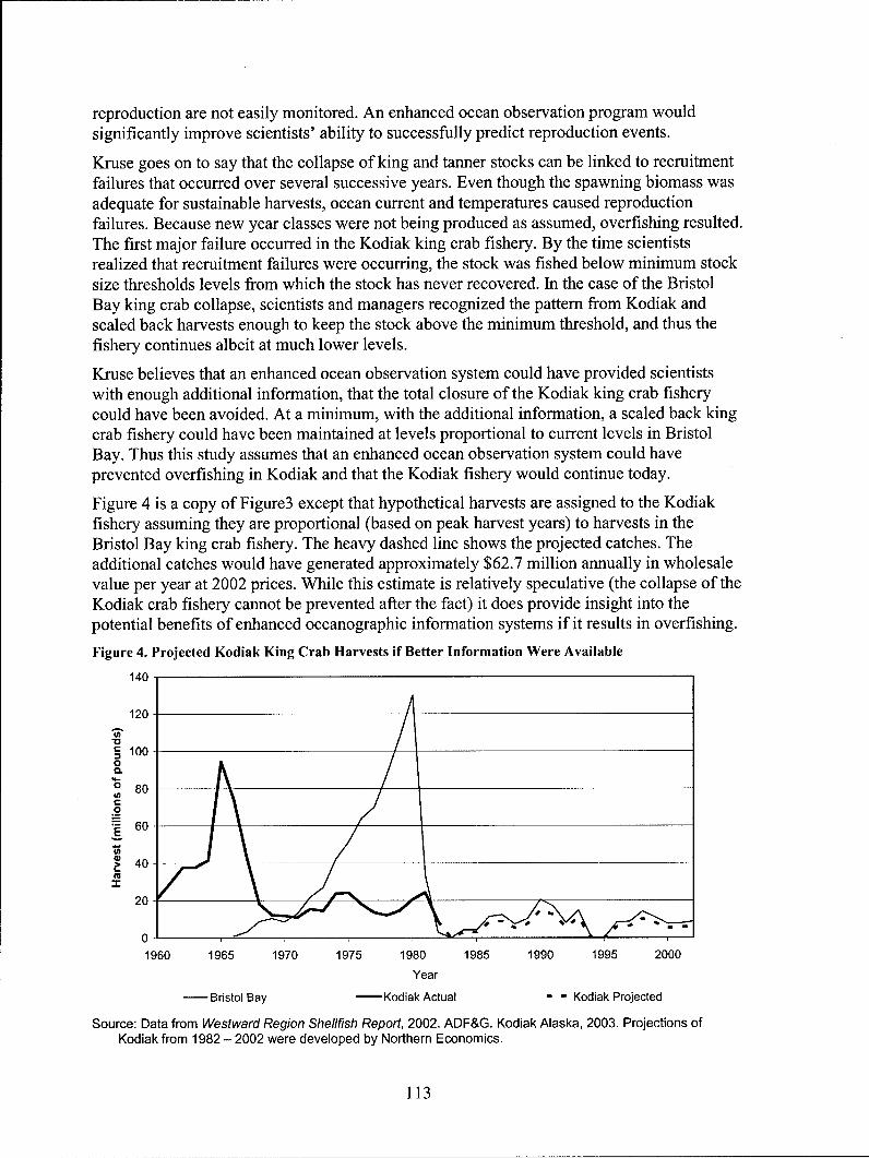
reproduction are not easily monitored. An enhanced ocean observation program wouldsignificantly improve scientists' ability to successfully predict reproduction events.
Kruse goes on to say that the collapse of king and tanner stocks can be linked to recruitmentfailures that occurred over several successive years. Even though the spawning biomass wasadequate for sustainable harvests, ocean current and temperatures caused reproductionfailures. Because new year classes were not being produced as assumed, overfishing resulted.The first major failure occurred in the Kodiak king crab fishery. By the time scientistsrealized that recruitment failures were occurring, the stock was fished below minimum stocksize thresholds levels from which the stock has never recovered. In the case of the BristolBay king crab collapse, scientists and managers recognized the pattern from Kodiak andscaled back harvests enough to keep the stock above the minimum threshold, and thus thefishery continues albeit at much lower levels.
Kruse believes that an enhanced ocean observation system could have provided scientistswith enough additional information, that the total closure of the Kodiak king crab fisherycould have been avoided. At a minimum, with the additional information, a scaled back kingcrab fishery could have been maintained at levels proportional to current levels in BristolBay. Thus this study assumes that an enhanced ocean observation system could haveprevented overfishing in Kodiak and that the Kodiak fishery would continue today.
Figure 4 is a copy of Figure3 except that hypothetical harvests are assigned to the Kodiakfishery assuming they are proportional (based on peak harvest years) to harvests in theBristol Bay king crab fishery. The heavy dashed line shows the projected catches. Theadditional catches would have generated approximately $62.7 million annually in wholesalevalue per year at 2002 prices. While this estimate is relatively speculative (the collapse of theKodiak crab fishery cannot be prevented after the fact) it does provide insight into thepotential benefits of enhanced oceanographic information systems if it results in overfishing.
Figure 4. Projected Kodiak King Crab Harvests if Better Information Were Available
140
120
n loo-0Q.0 80
0
S60--
~40- __ _ _ _ _
20-
0-1960 1965 1970 1975 1980 1985 1990 1995 2000
Year
-Bristol Bay -Kodiak Actual- - Kodiak Projected
Source: Data from Westward Region Shellfish Report, 2002. ADF&G. Kodiak Alaska, 2003. Projections ofKodiak from 1982 - 2002 were developed by Northern Economics.
113
Conclusions
Our estimates of the potential value of an enhanced AOOS to Alaska commercial fisheriesinclude:
0 $77 million annually in increased net revenue in Alaska salmon fisheries,
0 $504 million annually in increased total wholesale value in Alaska groundfishfisheries, and
0 $63 million annually in lost wholesale value that might have been avoided.
These three types of improvement should not be viewed as additive. The groundfish figure isan estimate of increased value of total output to processors, of which perhaps 20 25%34 mightbe considered a net increase in revenues above costs to both harvesters and processors. Theremaining 75-80% represents economic impacts that potentially could be generatedthroughout the region. The estimate of benefits to the salmon industries reflects costreductions and higher output values, or a change in net revenues or producer surplus. Thevalue assigned to the crab fishery is an estimate of foregone output or avoided cost/losses ofwhich again, only 20-25 percent might be considered a net increase in revenues above coststo both processors and harvesters.
Furthermore it should be noted that in developing our estimates of the value of enhancedAOOS information we found it difficult to specify quantitative decision and physicaloutcome models. Many of the scientists we talked to were able to speculate about thebenefits of more/better defined and accessible AOOS data but were only in early stages ofconsidering how to add oceanographic parameters to their stockassessment/recruitment/escapement models. Regardless, these scenarios are very difficult tomodel due to the complexity of nonlinear interactions in biological systems and the broadarray of influential parameters. Development of management decision making that takesenvironmental, ecological and ecosystem effects into account will require considerableamounts of monitoring, understanding of the behavioral relations among fishers, the fish theycatch and the prey of the harvested species (Langton and Haedrich, 1997). As such ouranalysis takes a significant leap between decisions to open or close a fishery and economicoutcomes and it is difficult to say, therefore, with confidence that additional biological andoceanographic data generated through enhanced AOOS will with complete certainty lead tobetter decision outcomes in fisheries management. In addition, in the long term, as thecomplexity of information requested from fisheries scientists increases, and as more andmore complex models are utilized, predictability and certainty may not necessarily increase.In fact, the more complex the models, the more they have to depend, in practice, onassumptions and presumptions rater than data. This may have implications for the value ofinformation provided by AOOS overtime.
34 The 20-25 percent is a rule of thumb estimate of the portion of total output that is likely tobe considered a "return on investment" by owners of the processing facilities and harvestingvessels, after fixed (including facility maintenance and replacement of production units--e.g.machinery, engines, etc) and variable costs.
114
That said, in the spirit of this project, as illustrated in the previous sections, we haveattempted to estimate the benefits that improvements in AOOS could generate. In particularwe have shown that enhanced AOOS could generate over $500 million annually in additionalvalue in select Alaska's commercial fisheries (e.g. Alaska groundfish fisheries). However,there are several factors, as explicitly outlined below, that may lead to the uncertainty aroundthose estimates.
1) It is unknown whether the proposed changes to the ocean observation program willactually deliver more and "better" data.
2) Assuming better data is delivered, it is unknown whether or when those data will beintegrated into stock assessment and run forecast models.
3) Assuming better data are integrated into the models it is unknown whether the newdata will actually improve the reliability of the models.
4) Assuming the reliability of the models is improved, it is unknown whether or whenthe improvements will be accepted by managers or industry members.
These types of uncertainties lead to a more conservative expected value of informationestimate. To assess benefits to the Alaska groundfish fishery, for example, of enhanced data,a value of information model (using hypothetical probabilities) might be expressed asfollows:
1) There is a 75% probability that groundfish scientists will be able to use the data torefine their analyses
2) There is a 50% probability that what scientists think today will be borne out by theirfurther analyses and data
3) There is a 50% probability that the NPFMC and NOAA NMFS will lift the 2 millionMT TAC cap, once a track record is established
4) There is a 50% probability that groundfish stocks will be in the same shape they arein 25 years from now
An expected value model combines the above probabilities multiplicatively. Thus based onthe hypothetical probabilities described above, there is only a 9 percent chance (0.75 x 0.5 x0.5 x 0.5), that the improvements generating $504 million (in today's dollars) will berealized.
In addition to the probabilistic model described above, the fact that the benefits of theenhanced ocean observation system are not expected to be realized for many years after thesystem is upgraded means that the cost and benefits stream must be discounted to presentvalues. If we assume conservatively, for example, that:
1) The cost of the observation system upgrades in Alaska are $100 million and occur in2005,
2) The cost of operating and maintaining the system for the next 50 years (until 2055)are $10 million per year,
3) The benefits of the program to the groundfish fishery ($504 million per year) begin toaccrue 15 years (in 2020) after the system is upgraded and continue until 2055,
115
4) The social discount rate is 7.5 percent;
Given the above assumptions, the net present value of enhancements to AOOS to Alaskagroundfish fisheries is reduced to only $17.5 million. If we further assume there is only a 9percent probability that the benefits of an enhanced system for the groundfish fishery will berealized then, the net present value becomes negative.
Transferability of Models and Results
While the approach taken in this analysis may be transferred to other fisheries around theU.S. it is not necessarily appropriate to transfer the estimates generated. Fisheries around thenation are each unique and managed as such. In addition the uncertainties inherent in value ofinformation models across fisheries will be unique. We have learned that the complexity ofthe biological and stock assessment models that are the basis for harvest rates and fisheriesmanagement generally make it very difficult to transfer applications even between fisherieswithin a region. We believe that best approach to modeling the value of enhanced COOS tofisheries across the United States will be through explicit case examples that illustrate thesign and potential magnitude of benefits.
116
Literature Reviewed and or Cited
ADF&G, 2004a. Bristol Bay Historical Information from ADF&G Division of CommercialFisheries at www.cf.adfg.state.ak.us. Accessed June 2004.
ADF&G Commercial Operator Annual Report Data, provided by ADF&G in June 2004.
ADF&G, 2003. Westward Region Shellfish Report, 2002. Kodiak Alaska, 2003.
The Bering-Aleutian Salmon International Survey (BASIS) Working Group.http://www/npafc.org/BASIS.
Burgner, R.L. 1980. Some Features of the Ocean Migrations and Timing of Pacific Salmon.Pp. 153-163. In Salmonid Ecosystems of the North Pacific. W.J. McNeil and D.C.Himsworth (eds), Oregon State University Press, Corvallis, Oregon.
Commercial Fishing Entry Commission, 2004. Basic Information Tables, from internet site atwww.cfec.state.ak.us. Accessed in June 2004
Gardiner, Terry, 2004. President of Norquest Seafoods. Personal Communication withNorthern Economics, Inc. May 2004.
Giles, Don, 2004. President Icicle Seafoods. Personal Communication with NorthernEconomics, Inc. May 2004.
Goodman, D. et al. 2002. Scientific Review of the Harvest Strategy Currently Used in theBSAI and GOA Groundfish Fishery Management Plans. Report Prepared for the NorthPacific Fishery Management Council.
Hakoyama, H. and W. Sakamoto. 1995. Pink salmon migration in relation to sea surfacetemperature and day length in the open sea. Nippon Suisan Gakkaishi 61(2):137-141.
Hamlet, A.F., D. Huppert, and D.P. Lettenmaier. 2001. Economic Value of Long-LeadStreamflow Forecasts for Columbia River Hydropower. Report Submitted to theBonneville Power Administration.
Hiatt, Terry, Ron Felthoven, Chang Seung, and Joe Terry. 2003. Economic Status of theGroundfish Fisheries off Alaska, 2002. Alaska Fishery Science Center, National MarineFisheries Service, National Oceanic and Atmospheric Administration, US Department ofCommerce. Seattle, Washington. November 2003.
lanelli, James, 2003. "North Pacific Multi-Species Management Model", in Appendix H toAlaska Groundfish Fisheries, Final Programmatic Supplemental Environmental ImpactStatement. National Marine Fisheries Alaska Region. Juneau Alaska. June 2004.
Janelli, Dr. James, 2004. Fishery Scientist, Alaska Fishery Science Center, National MarineFisheries Services. Personal Communication with Northern Economics, Inc. May 2004.
Kruse, G., D.M. Eggers, R.J. Marasco, C. Pautzke, and T.J. Quinn (editors). 1993.Proceedings of the International Symposium on Management Strategies for ExploitedFish Populations. Alaska Sea Grant College Program Report No 93-02. University ofAlaska, Fairbanks.
117
Kruse, Gordon, 2004. Chief Scientist with ADF&G. Personal Communication with NorthernEconomics, Inc., May 2004..
Link, Michael, et Al., 2003. An Analysis of Options to Restructure the Bristol Bay SalmonFishery. Prepared for the Bristol Bay Economic Development Corporation. DillinghamAlaska. March 2003.
Mikol, B. 1997. Temperature Directed Fishing: How to Reduce Bycatch and IncreaseProductivity. University of Alaska Sea Grant College Program Marine Advisory BulletinNo. 48.
Mundy, P.R. 1982. Computation of migratory timing statistics for adult Chinook salmon inthe Yukon River, Alaska and their relevance to fisheries management. N. AmericanJournal of Fisheries Management. 4:359-370.
Northern Economics, Inc. 2003. Impact of the Seafood Industry on Alaska's Economy.Prepared for Pacific Seafoods Processors Association. Juneau AK.
NMFS, 2003. Fisheries of the United States, 2002. National Marine Fisheries Service, Officeof Science and Technology, Fisheries Statistics and Economics Division. Silver Spring,MD. NMFS 2004. Alaska Groundfish Fisheries Final Programmatic SupplementalEnvironmental Impact Statement.
National Marine Fisheries Alaska Region, National Oceanic and AtmosphericAdministration, US Department of Commerce. Juneau Alaska. June 2004.
NPFMC, 2004. Annual AFA Cooperative Reports. Submitted to the North Pacific FisheryManagement Council. Anchorage, AK
NPFMC, 2002. Impacts of the American Fisheries Act. Report to the US Congress and theSecretary of Commerce. February 2002.
Stasko, A.B. et al. 1973. Migration Orientation of Atlantic salmon. International SalmonSymposium. 1972. International Atlantic Salmon Foundation, Special Publication.4(l):119-137.
Solow, A.R. et al. 1998. The Value of Improved ENSO Prediction to U.S. Agriculture.Climate Change 39:47-60.
The U.S. Integrated Ocean Observing System (IOOS) Plan for Data Management andCommunications (DMAC). Part III. Appendices, Appendix 4: User Outreach. IOOSDMAC User Outreach Team. September 30, 2003.
Willette, M. T., and W.S. Pegau. 2004. Monitoring Dynamics of the Alaska Coastal Currentand Development of Applications for Management of Cook Inlet Salmon. Proposalsubmitted to Exxon Valdez Oil Spill Trustees.
Wilson, B. and G. Tomlins. 1999. Mapping Cook Inlet rid tides using local knowledge andremote sensing. Pages 1-10. In Proceedings of the Cook Inlet Oceanography Workshop.M.A. Johnson and S.R. Okkonen (eds.), University of Alaska, Fairbanks, Alaska.
Van Vacter, Norm, 2004. Dillingham Plant Manager, Peter Pan Seafoods. PersonalCommunication with Northern Economics, Inc. May 2004.
118

Appendix D: Recreational Boating on the Great Lakes
Tom PelsociDelta Research Corp.
119
DECISION MODEL
TO ESTIMATE THE VALUE OF IMPROVED WAVE HEIGHT FORECASTS FOR
GREAT LAKES RECREATIONAL BOATING
Case StudyCoordinated Regional Benefit Studies of Coastal Ocean Observing Systems
(Great Lakes Region)
Tom PelsociDelta Research Corp.
Chicago, Illinois
June 30, 2004
Funded through the National Ocean Partnership Program, supported by the NationalOceanic and Atmospheric Administration, National Science Foundation, Office of NavalResearch, U.S. Environmental Protection Agency, US Geological Survey, MineralManagement Service, U.S. Coast Guard, Defense Advanced Research Projects Agency,Department of State, the U.S. Army Corps of Engineers, and the National Aeronautics &Space Administration.
120
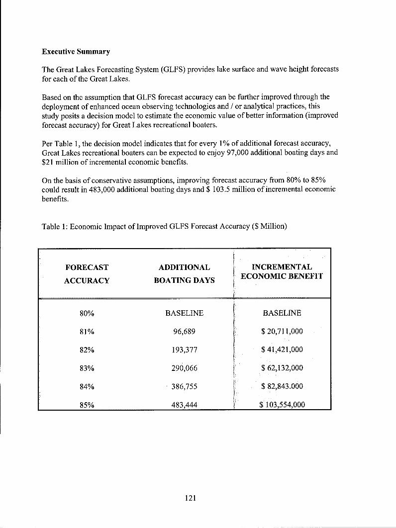
Executive Summary
The Great Lakes Forecasting System (GLFS) provides lake surface and wave height forecastsfor each of the Great Lakes.
Based on the assumption that GLFS forecast accuracy can be further improved through thedeployment of enhanced ocean observing technologies and / or analytical practices, thisstudy posits a decision model to estimate the economic value of better information (improvedforecast accuracy) for Great Lakes recreational boaters.
Per Table 1, the decision model indicates that for every 1% of additional forecast accuracy,Great Lakes recreational boaters can be expected to enjoy 97,000 additional boating days and$21 million of incremental economic benefits.
On the basis of conservative assumptions, improving forecast accuracy from 80% to 85%could result in 483,000 additional boating days and $ 103.5 million of incremental economicbenefits.
Table 1: Economic Impact of Improved GLFS Forecast Accuracy ($ Million)
FORECAST ADDITIONAL INCREMENTAL
ACCURACY BOATING DAYS ECONOMIC BENEFIT
80% BASELINE BASELINE
81% 96,689 $ 20,711,000
82% 193,377 $ 41,421,000
83% 290,066 $ 62,132,000
84% 386,755 $ 82,843.000
85% 483,444 $ 103,554,000
121
Wave Phenomena and Wave Forecasts
Discussions with marina operators, staff of recreational boating associations, and editors ofrecreational boating journals and outlets indicate that weather forecasts are considered to bevery important by Great Lakes recreational boaters. In particular wave heights and waveperiodicity (choppiness) are key concerns relative to safety and enjoyment.
While the type of vessel (sailing vs. motor boat), the size of the vessel, and the skill andexperience of the operator are important sources of variation, expert input would indicate thatin seas with 18" wave heights and higher, coupled with choppy conditions, amateur sailorsand motor boaters will have a less than pleasurable experience and may find conditionsunsafe.
Since recreational motorboats are generally less seaworthy than sailing vessels and are "madeto go fast", wave height is a particularly important constraint relative to enjoyable recreation.We therefore posited that
"- "Good" surface conditions are associated with wave heights under 18" and- "Bad" surface conditions are associated with wave heights at or over 18".
Wave height along with wave periodicity information is forecasted by the NOAA GreatLakes Forecasting System (GLFS), on an hourly basis, for a 5 km grid (except for LakeSuperior where the grid is 10 kin).
The initial implementation of the GLFS for Lake Erie was completed in 1993. GLFS hassince been extended to the other four Great Lakes. GLFS operates with two components (1)an atmospheric input module (a step coordinate Eta model) to force a (2) numerical oceanmodule (Princeton Ocean Model).
Great Lakes marine forecasting is relatively difficult due to "the presence of small scalecoastal features which can generate local convergence / divergence regions and the presenceof strong air-lake fluxes, rapid upwelling, and seiches. The Great Lakes Forecasting Systemuses the output from the Eta model as input to the wave or ocean model and there is nofeedback between the waves that develop and the winds that generate them" (Sousounis).
Wave Height Observations
The National Buoy Data Center (NBDC) operates 12 moored buoys in coastal and offshorewaters of the five Great Lakes. Additional surface information is also collected by on-shoreC-MAN stations (Figure 1)
122
Figure 1: Great Lakes Surface Data Collected by NDBC Buoy's
21C -- -""-
,~A
WSCNSIN MICHIGANtI
'NEW YORK
U Moored Buoys
A C- MAN Stations
Based on NDBC 1981 to 2001 time-series of empirically observed wave patterns, thearithmetic mean wave heights for the Great Lakes during the five and half month recreationalboating season have a tendency to exceed 18 inches 70 percent of the time (Table 2).
Table 2: Mean Wave Heights for Great Lakes May 1- October 15, 1981-2001 (inches)OCT
MAY JUNE JULY AUGUST SEPT (1-15)Lake Erie -Sandusky 15.76 11.82 15.76 19.7 27.58 31.52
Lake MichiganSouth 15.76 11.82 19.7 23.64 35.46 39.4Lake MichiganNorth 19.7 15.76 19.7 23.64 35.46 43.34
Lake HuronCentral 19.7 15.76 19.7 23.64 35.46 43.34Lake SuperiorCentral 19.7 15.76 11.82 19.7 35.46 47.28
Source: National Data Buoy Center, Historical Time Series
123
However, when reviewing actual (as opposed to mean wave heights), 2002 and 2003 hourlydata for three of the twelve NDBC buoys, only 40 percent of hourly readings (during theMay to October period) exceeded 18".
Since it can be further assumed that the bulk of recreational boating takes place during themonths of June, July, and August, hourly readings for these 3 months indicate that waveheight exceeds 18" only 31.5 percent of the time.
Accordingly, on the basis of the above empirical evidence, we assumed that lake
surface conditions are "Good" 68.5 % of the time and "Bad" 31 .5 % of the time.
Decision Model and Physical Outcome Model
The following assumptions were used for a base-case decision model.
- GLFS forecasts are able to correctly identify "Good" lake surface conditions 80% ofthe time and fail to do so 20% of the time.
- GLFS forecasts are able to correctly identify "Bad" lake surface conditions 80% ofthe time and fail to do so 20% of the time.
- During subsequent analysis, forecast accuracy was deemed the independent variableand frequency of "Good" forecasts was stepped in 1% increments from 80% to 85%
In addition, three decision rules were posited to drive recreational boater behavior:
- Forecast of "Good" lake surface conditions will result in a decision to "go out" by100% of boaters, planning to go boating or inclined to go boating any particular day(this is equivalent to a condition of "all other things being equal".
- 15% of boaters who have appropriate expertise to navigate in difficult lake conditionsor who lack such expertise and recklessly ignore forecasts of "Bad" lake surfaceconditions and "go out" anyway.
- 85% of boaters, who tend to be more cautious or realize that "Bad" wave conditionsdo not make for an enjoyable experience, will act in conformity with availableforecasts. When the forecast indicates "Bad" lake surface condition, these 85% ofboaters will stay in harbor.
Finally, as "the Great Lakes Forecasting System uses outputs from the Eta model as input tothe wave (or ocean) model and there is no feedback between the waves that develop and thewinds that generate them" (Sousounis), for purposes of modeling recreational boater
124
behavior, we assumed a condition of independence between wave forecasts and observedwave conditions.
Reflecting the above assumptions, a base-case decision model is indicated in Figure
2.
As forecast accuracy is incremented (relative to a base case decision model) for each onepercent improvement in forecast accuracy, the probability of the combination "Good"Surface Conditions - Incorrect Forecast - Decision to Stay in Harbor (i.e., the probability oflost boating days) decreases as indicated in Table 3
Figure 2: Decision Model, Boater Behavior as Function of Forecast Accuracy
Wave Height Wave Wave Decision Boater Probability(Empirically Forecast Forecast Parameter Behavior of PhysicalObserved and Accuracy (Physical OutcomeGiven) (Independent Outcome)
Variable)
0.15 Go Out Anyway 0.0378
Correct F/C0.80
"Bad" 18" 5 Stay in Harbor 0.2142
(0.315)
0.20 Incorrect F/C Follow F/C & Go Out 0.0630-100
0.80 Correct F/C Follow F/C & Go Out 0.54801.00
"Good"
Under 18"(0.685) Incorrect F/, 0.15 Go Out Anyway 0.02055
Incorrect F/C
"Stay in Harbor 0.11645Forego EnjoyableBoating Day
125
Table 3: Improving Forecast Accuracy and the Probability of Lost Boating Days
Forecast Accuracy Probability of Lost Boating DaysBase-case 80% 0.11645
81% 0.110627582% 0.10480583% 0.098982584% 0.0931685% 0.0873375
Economic Outcome Model
The Economic Outcome Model incorporates the following additional assumptions:
- For Michigan, Ohio, Wisconsin, and Illinois, Great Lakes boating days are derivedfrom the number of recreational boats registered statewide. It is assumed that theseboats average 12.1 boating days per year (NSRE) and that 50 percent of boating daysare spent on the Great Lakes, as opposed to rivers and smaller lakes.
- For New York, Pennsylvania, Indiana and Minnesota, boating days are derived fromthe number of boats registered in Great Lake coastal counties. It is assumed that theseboats average 12.1 boating days per year (NSRE) and that 90% of boating days arespent on the Great Lakes. This adjustment is due to the extensive saltwatercomponent in New York and Pennsylvania and to the very large internal (non-GreatLake) component in Indiana and Minnesota.
- Based on the above approach, boating days for the five Great Lakes are estimated at16.6 million days per year (Table 4, Column 4).
Based on a 1999 Study of the economic impact of recreational boating in Ohio (Hushak),daily expenses for travel, meals, boat-fuel, marina fees, etc. are assumed to average $187 perday for all Great Lakes boating days. This average value excludes capital investments forboat acquisition and major upgrades and is adjusted to 2003 dollars to yield $ 214 per day.
126
Table 4: Economic Impact as a Function of Forecast AccuracyForecast Probability Delta: Great Increase Average EconomicAccuracy of Lost Decreased Lakes in Great Value of Benefits
Boating Probability Boating Lakes Boating fromDays Lost Days Days Per Boating Day ($) Improved
Year Days Forecasts)(1) ((2) (3) (4) (5) (6) (7)
80% 0.11645 0 16,606,049 0 214.2 0
81% 0.1106275 0.0058225 16,606,049 96,689 214.2 $ 20,711,000
82% 0.104805 0.011645 16,606,049 193,377 214.2 $ 41,421,000
83% 0.0989825 0.0174675 16,606,049 290,066 214.2 $ 62,132,000
84% 0.09316 0.02329 16,606,049 386,755 214.2 $ 82,843,000
85% 0.0873375 0.0291125 16,606,049 483,444 214.2 $ 103.55mill
Table 4, Columns 5 and 7 indicate that for every 1% of additional wave height forecastaccuracy, Great Lakes recreational boaters are likely to enjoy 97,000 additional boating dayscorresponding to $21 million in incremental economic benefits.
On the basis of conservative assumptions, improving current wave height forecast accuracyfrom 80% to 85% would thereby generate 483,000 additional boating days and $103.5million of incremental economic benefits.
Applicability to Other Regions
The above approach may be applied to other coastal regions if the assumptions, appropriatefor the Great Lakes region, are adjusted to reflect conditions in other coastal regions. Inparticular,
- Assumptions about feedback loops in ocean surface forecasting systems,- Wave height time-series observations for a relevant recreational season,- Assumptions about number of boating days and the value of boating days, etc.
127
References
Great Lakes Commission. 2000. Recreational Boating and the Great Lakes - St.Lawrence Region.
Gunderson, J. and Kreag, G., 1990, Estimated Economic Impact of Recreational Fishingon Minnesota Waters of Lake Superior, Minnesota SeaGrant. Minneapolis MN.
Hushak, L. 1999. Recreational Boating in Ohio: An Economic Impact Study. OhioSeaGrant Publication. Columbus OH.
Leeworthy,V. and Wiley, P. 2001. Current Participation Patterns in Marine RecreationNational Survey on Recreation and the Environment 2000. National Oceanic andAtmospheric Administration. Washington, DC.
National Marine Manufacturers Association, 2000, 1999 U.S. Recreational BoatRegistration Statistics.
National Survey on Recreation and the Environment. 2000. National Oceanographic andAtmospheric Administration. Washington DC.
NMFS or National Marine Fishery Service. 2001. Marine Recreation FishingExpenditure Survey < http://www.st.nmfs.gov/stl/econ/implan.pdf >
Sousounis, P. Improving Marine Forecasts Over the Great Lakes The Comet Outreach
Program, < http://www.comet.ucar.ed/outreach/991 5807. htm >
Schwab, D. J., et. al., February 1999. Forecast Verification for Eta Model Winds UsingLake Erie Storm Surge Water Levels. Weather and Forecasting
Schwab, D. J. and Bedford, K.W. 1999. "The Great Lakes Forecasting System" Coastaland Estuary Studies 56, pages 157-173. American Geophysical Union.
Wisconsin SeaGrant, 2003, Coastal Business and Economic Development,< http://seagrant/wisc.edu/greatlakes/glnetwork/economic.html >
U.S. Coast Guard (U.S. Department of Transportation), 2000, Boating Statistics 2000,Comdtpub P 16754.14
Vilaplana, J. and Hushak, L. 1999. Outdoor Recreation at Lake Erie. Ohio Sea GrantProgram. Columbus, OH.
128
50272-101
REPORT DOCUMENTATION 1 REPORT NO. 2. 3. Recipient's Accession No.
PAGE WHOI-2005-03
4. Title and Subtitle 5. Report Date
Estimating the Economic Benefits of Regional Ocean Observing Systems April 20056.
7.Author(s)Hauke L. Kite-Powell, Charles S. Colgan, Katharine F. Wellman, 8. Performing Organization Rept. No.
Thomas Pelsoci. Kenneth Wieand. Linwood Pendleton. Mark I. Kaiser. WHOI-2005-039. Performing Organization Name and Address 10. ProJectfraskiWork Unit No.
Woods Hole Oceanographic Institution 11. Contract(C) or Grant(G) No.
Woods Hole, Massachusetts 02543 (c) N00014-02-1-1037
(G)
12. Sponsoring Organization Name and Address 13. Type of Report & Period Covered
Office of Naval Research Technical Report
14.
15. Supplementary Notes
This report should be cited as: Woods Hole Oceanog. Inst. Tech. Rept., WHOI-2005-03.
16. Abstract (Limit: 200 words)
We develop a methodology to estimate the potential economic benefits from new investments in regionalcoastal ocean observing systems in US waters, and apply this methodology to generate preliminary estimatesof such benefits. The approach focuses on potential economic benefits from coastal ocean observinginformation within ten geographic regions encompassing all coastal waters of the United States, and withina wide range of industrial and recreational activities including recreational fishing and boating, beachrecreation, maritime transportation, search and rescue operations, spill response, marine hazardsprediction, offshore energy, power generation, and commercial fishing. Our findings suggest that annualbenefits to users from the deployment of ocean observing systems are likely to run in the multiple $100s ofmillions of dollars per year. The project results should be considered first-order estimates that are subjectto considerable refinement as the parameters of regional observing systems are better defined, and as ourunderstanding of user sectors improves.
17. Document Analysis a. Descriptors
ocean observing systemeconomic benefitscoastal ocean
b. Identifiers/Open-Ended Terms
c. COSATI Field/Group
18. Availability Statement 19. Security Class (This Report) 21. No. of PagesUNCLASSIFIED 139
Approved for public release; distribution unlimited. UrCLASS ( a.20. Security Class (This Page) 22. Price
(See ANSI-Z39.18) See Instructions on Reverse OPTIONAL FORM 272 (4-77)(Formerly NTIS-35)Department of Commerce

DOCUMENT LIBRARYDistribution List for Technical Report Exchange - July 1998
University of California, San Diego Fisheries-Oceanography LibrarySIO Library 0175C 151 Oceanography Teaching Bldg.
9500 Gilman Drive University of Washington
La Jolla, CA 92093-0175 Seattle, WA 98195
Hancock Library of Biology & Oceanography LibraryAlan Hancock Laboratory R.S.M.A.S.
University of Southern California University of MiamiUniversity Park 4600 Rickenbacker Causeway
Los Angeles, CA 90089-0371 Miami, FL 33149
Gifts & Exchanges Maury Oceanographic LibraryLibrary Naval Oceanographic OfficeBedford Institute of Oceanography Building 1003 SouthP.O. Box 1006 1002 Balch Blvd.Dartmouth, NS, B2Y 4A2, CANADA Stennis Space Center, MS, 39522-5001
NOAA/EDIS Miami Library Center Library4301 Rickenbacker Causeway Institute of Ocean SciencesMiami, FL 33149 P.O. Box 6000
Research Library Sidney, B.C. V8L 4B2
U.S. Army Corps of Engineers CANADA
Waterways Experiment Station National Oceanographic Library3909 Halls Ferry Road Southampton Oceanography CentreVicksburg, MS 39180-6199 European Way
Marine Resources Information Center Southampton S014 3ZH
Building E38-320 UK
MIT The LibrarianCambridge, MA 02139 CSIRO Marine Laboratories
Library G.P.O. Box 1538Lamont-Doherty Geological Observatory Hobart, TasmaniaColumbia University AUSTRALIA 7001
Palisades, NY 10964 Library
Library Proudman Oceanographic LaboratorySerials Department Bidston ObservatoryOregon State University BirkenheadCorvallis, OR 97331 Merseyside L43 7 RA
Pell Marine Science Library UNITED KINGDOM
University of Rhode Island IFREMERNarragansett Bay Campus Biblioth~que La P~rouseNarragansett, RI 02882 Centre de Documentation sur la Mer
Working Collection 15 rue Dumont d'Urville
Texas A&M University Technop6le Brest-Iroise
Dept. of Oceanography BP 70 - 29280 Plouzan6 - FRANCE
College Station, TX 77843