Statistical Methodology 2 (2005) 121–130

www.elsevier.com/locate/stamet

Estimating parameters of a selected Paretopopulation

Somesh Kumara,∗, Aditi Kar Gangopadhyayb

aDepartment of Mathematics, Indian Institute of Technology, Kharagpur-721302, IndiabDepartment of Mathematics, Indian Institute of Technology, Roorkee-247667, India

Received 29 October 2004

Abstract

Let Π1, . . . ,Πk be k populations withΠi being Pareto with unknown scale parameterαi andknown shape parameterβi ; i = 1, . . . , k. Suppose independent random samples(Xi1, . . . , Xin),i = 1, . . . , k of equal size are drawn from each ofk populations and letXi denote the smallestobservation of thei th sample. The population corresponding to the largestXi is selected. We considerthe problem of estimating the scale parameter of the selected population and obtain the uniformlyminimum variance unbiased estimator (UMVUE) when the shape parameters are assumed to beequal. An admissible class of linear estimators is derived. Further, a general inadmissibility result forthe scale equivariant estimators is proved.© 2005 Published by Elsevier B.V.

Keywords: Selection rule; UMVUE; Admissibility; Scale equivariant estimator; Brewster–Zidek technique

1. Introduction

Let Π1, . . . ,Πk be k Pareto populations withΠi having an associated probabilitydensity given by

fi (x) = βi αβii

xβi +1, x ≥ αi , βi > 0, i = 1, . . . , k (1.1)

∗ Corresponding author. Tel.: +91 3222 283662; fax: +91 3222 255303.E-mail addresses:smsh@iitkgp.ac.in, smsh@indiatimes.com (S. Kumar).

1572-3127/$ - see front matter © 2005 Published by Elsevier B.V.doi:10.1016/j.stamet.2005.02.001

122 S. Kumar, A.K. Gangopadhyay / Statistical Methodology 2 (2005) 121–130

where scale parametersαi ’s are unknown and shape parametersβi ’s are assumed to beknown. Suppose we have random samples(Xi1, . . . , Xin), i = 1, . . . , k from populationsΠ1, . . . ,Πk respectively. Further, letXi = min(Xi1, . . . , Xin), i = 1, . . . , k. Our aim isto select the population corresponding to the largestαi , i = 1, . . . , k. The statistic X =(X1, . . . , Xk) is complete and sufficient and thedensity ofXi has the monotone likelihoodratio property in(αi , Xi ). A natural selection rule is to select the population correspondingto the largestXi , i = 1, . . . , k, that is,Πi is selected ifXi = max{X1, . . . , Xk}. Optimalityproperties of the natural selection rule have been investigated by Bahadur and Goodman[2], Lehmann [17] and Eaton [9]. In this paper we consider the problemof estimating thescale parameter of the selected Pareto population.

The problem of estimation after selection has received considerable attention of manyresearchers in the recent past. This type of problem arises in various agricultural, industrial,medical or economic experiments. For example, acommercial vehicle operator will preferto buy a vehicle with maximum fuel efficiency. He will also be interested in having anestimate of the average fuel efficiency of the selected vehicle. Dahiya [7], Hsieh [13] andCohen and Sackrowitz [6] have proposed various estimators for estimating the mean ofthe selected normal population. For the results on nonnormal populations one may refer toSackrowitz and Samuel-Cahn [21], Kumar and Kar [16], Vellaisamy et al. [23], Vellaisamyand Sharma [24], Vellaisamy [22] and Misra and van der Meulen [19] who have studiedthis problem for negative exponential, uniform, gamma and general truncatation parameterdistributions.

The Pareto distribution was initially used by Pareto [20] to study income distributions.Since then it has found applications in a variety of industrial, engineering and economicstudies. Several such situations have been discussed by Johnson and Kotz [14], Harris [11],Davis and Feldstein [8], Freiling [10], and Berger and Mandelbrot [3]. They have usedthe Pareto distribution for describing the distribution of city maintenance service times,nuclear fallout particle distribution, and the distribution of error clusters in communicationcircuits, etc. For a review of literature on estimating parameters of Pareto populations onemay refer to the papers by Charek et al. [5], Malik [ 18], Kern [15], Hosking and Wallis[12] and Asrabadi [1].

In this paper, we consider estimation of the scale parameterαJ of the selected Paretopopulation when the shape parametersβi ’s areknown. InSection 2, we derive theUMVUEwhen theβi ’s are equal. InSection 3, an admissible class of linear estimators isobtained.In Section 4, we provea general inadmissibility result for the scale equivariant estimators.

2. Existence of UMVUE of αJ for common shape parameters

We estimate the scale parameterαJ of the selected population when the shapeparametersβi ’s areknown. So, the parameter of interest isαJ , whereJ = i , if Xi ≥X j ,∀ j �= i , j = 1, . . . , k, i = 1, . . . , k.

In this section, the case of two populations with common shape parameterβ isconsidered. We use a heuristic approach to derive an unbiased estimator and consequentlythe UMVUE ofαJ in the following theorem.

S. Kumar, A.K. Gangopadhyay / Statistical Methodology 2 (2005) 121–130 123

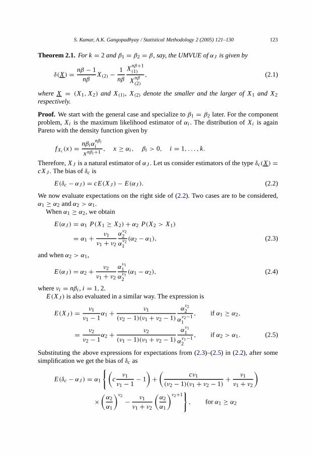
Theorem 2.1. For k = 2 andβ1 = β2 = β, say, the UMVUE ofαJ is given by

δ(X) = nβ − 1

nβX(2) − 1

nβ

Xnβ+1(1)

Xnβ(2)

, (2.1)

where X = (X1, X2) and X(1), X(2) denote the smaller and the larger of X1 and X2respectively.

Proof. We start with the general case and specialize toβ1 = β2 later. For the componentproblem,Xi is the maximum likelihood estimator ofαi . Thedistribution of Xi is againPareto with the density function given by

fXi (x) = nβi αnβii

xnβi +1, x ≥ αi , βi > 0, i = 1, . . . , k.

Therefore,XJ is a natural estimator ofαJ . Let usconsider estimators of the typeδc(X) =cXJ . Thebias ofδc is

E(δc − αJ) = cE(XJ) − E(αJ). (2.2)

We now evaluate expectations on the right side of (2.2). Two cases are to be considered,α1 ≥ α2 andα2 > α1.

Whenα1 ≥ α2, weobtain

E(αJ) = α1 P(X1 ≥ X2) + α2 P(X2 > X1)

= α1 + ν1

ν1 + ν2

αν22

αν21

(α2 − α1), (2.3)

and whenα2 > α1,

E(αJ) = α2 + ν2

ν1 + ν2

αν11

αν12

(α1 − α2), (2.4)

whereνi = nβi , i = 1, 2.E(XJ) is also evaluated in a similar way. The expression is

E(XJ) = ν1

ν1 − 1α1 + ν1

(ν2 − 1)(ν1 + ν2 − 1)

αν22

αν2−11

, if α1 ≥ α2,

= ν2

ν2 − 1α2 + ν2

(ν1 − 1)(ν1 + ν2 − 1)

αν11

αν1−12

, if α2 > α1. (2.5)

Substituting the above expressions for expectations from (2.3)–(2.5) in (2.2), after somesimplification we get the bias ofδc as

E(δc − αJ) = α1

{(c

ν1

ν1 − 1− 1

)+(

cν1

(ν2 − 1)(ν1 + ν2 − 1)+ ν1

ν1 + ν2

)

×(

α2

α1

)ν2

− ν1

ν1 + ν2

(α2

α1

)ν2+1}

, for α1 ≥ α2

124 S. Kumar, A.K. Gangopadhyay / Statistical Methodology 2 (2005) 121–130

= α2

{(c

ν2

ν2 − 1− 1

)+(

cν2

(ν1 − 1)(ν1 + ν2 − 1)+ ν2

ν1 + ν2

)

×(

α1

α2

)ν1

− ν2

ν1 + ν2

(α1

α2

)ν1+1}

, for α2 > α1. (2.6)

The appearance of terms(

α2α1

)ν2,(

α2α1

)ν2+1,(

α1α2

)ν1and

(α1α2

)ν1+1in the bias expression

suggests that in order to get an unbiased estimator we should consider a function of the

typeX

c1(1)

Xc2(2)

, wherec1 andc2 are some constants to be chosen suitably. We now evaluate the

expectation of this term and obtain

E

(Xc1

(1)

Xc2(2)

)= ν1ν2

{α

c12

(ν2 − c1)(ν1 + c2)αc21

+(

1

(ν1 − c1)(ν2 + c2)

− 1

(ν1 − c1)(ν1 + ν2 + c2 − c1)− 1

(ν2 − c1)(ν1 + ν2 + c2 − c1)

)

αν22

αν2+c2−c11

}, if α1 ≥ α2. (2.7)

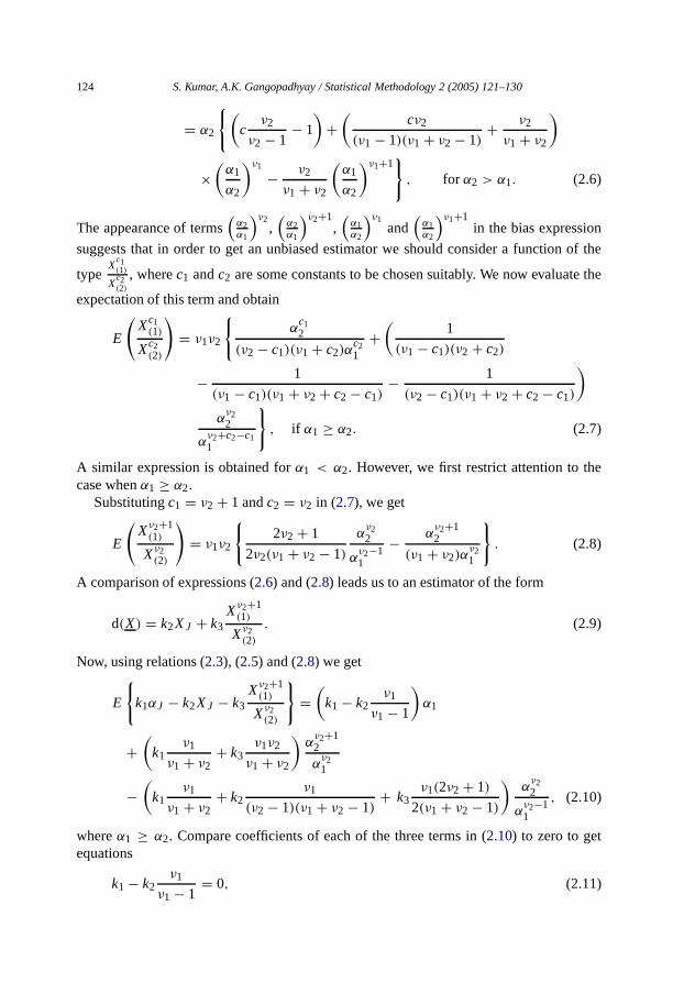
A similar expression isobtained forα1 < α2. However, we first restrict attention to thecase whenα1 ≥ α2.

Substitutingc1 = ν2 + 1 andc2 = ν2 in (2.7), we get

E

(Xν2+1

(1)

Xν2(2)

)= ν1ν2

{2ν2 + 1

2ν2(ν1 + ν2 − 1)

αν22

αν2−11

− αν2+12

(ν1 + ν2)αν21

}. (2.8)

A comparison of expressions (2.6) and (2.8) leads us to an estimator of the form

d(X) = k2XJ + k3Xν2+1

(1)

Xν2(2)

. (2.9)

Now, using relations (2.3), (2.5) and (2.8) we get

E

{k1αJ − k2XJ − k3

Xν2+1(1)

Xν2(2)

}=(

k1 − k2ν1

ν1 − 1

)α1

+(

k1ν1

ν1 + ν2+ k3

ν1ν2

ν1 + ν2

)α

ν2+12

αν21

−(

k1ν1

ν1 + ν2+ k2

ν1

(ν2 − 1)(ν1 + ν2 − 1)+ k3

ν1(2ν2 + 1)

2(ν1 + ν2 − 1)

)α

ν22

αν2−11

, (2.10)

whereα1 ≥ α2. Compare coefficients of each of the three terms in (2.10) to zero to getequations

k1 − k2ν1

ν1 − 1= 0, (2.11)

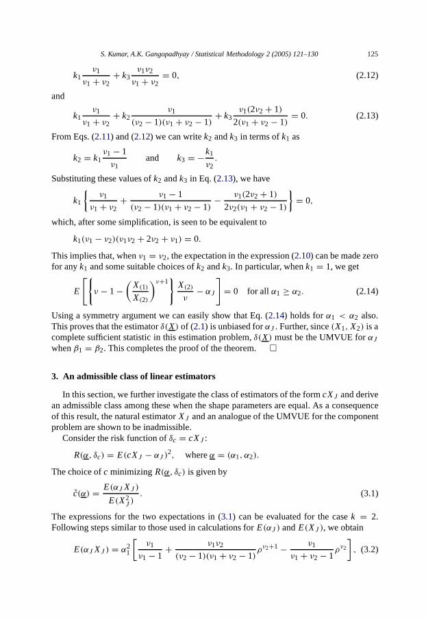
S. Kumar, A.K. Gangopadhyay / Statistical Methodology 2 (2005) 121–130 125

k1ν1

ν1 + ν2+ k3

ν1ν2

ν1 + ν2= 0, (2.12)

and

k1ν1

ν1 + ν2+ k2

ν1

(ν2 − 1)(ν1 + ν2 − 1)+ k3

ν1(2ν2 + 1)

2(ν1 + ν2 − 1)= 0. (2.13)

From Eqs. (2.11) and (2.12) we can writek2 andk3 in terms ofk1 as

k2 = k1ν1 − 1

ν1and k3 = −k1

ν2.

Substituting these values ofk2 andk3 in Eq. (2.13), we have

k1

{ν1

ν1 + ν2+ ν1 − 1

(ν2 − 1)(ν1 + ν2 − 1)− ν1(2ν2 + 1)

2ν2(ν1 + ν2 − 1)

}= 0,

which, after some simplification, is seen to be equivalent to

k1(ν1 − ν2)(ν1ν2 + 2ν2 + ν1) = 0.

This implies that, whenν1 = ν2, the expectation in the expression (2.10) can be made zerofor anyk1 and some suitable choices ofk2 andk3. In particular, whenk1 = 1, we get

E

[{ν − 1 −

(X(1)

X(2)

)ν+1}

X(2)

ν− αJ

]= 0 for all α1 ≥ α2. (2.14)

Using a symmetry argument we can easily show that Eq. (2.14) holds forα1 < α2 also.This proves that the estimatorδ(X) of (2.1) isunbiased forαJ . Further, since(X1, X2) is acomplete sufficient statistic in this estimation problem,δ(X) must be the UMVUE forαJ

whenβ1 = β2. This completes the proof of the theorem. �

3. An admissible class of linear estimators

In this section, we further investigate the class of estimators of the formcXJ and derivean admissible class among these when the shape parameters are equal. As a consequenceof this result, the natural estimatorXJ and an analogue of the UMVUE for the componentproblem are shown to be inadmissible.

Consider the risk function ofδc = cXJ :

R(α, δc) = E(cXJ − αJ)2, whereα = (α1, α2).

The choice ofc minimizing R(α, δc) is given by

c(α) = E(αJ XJ)

E(X2J)

. (3.1)

The expressions for the two expectations in (3.1) can be evaluated for the casek = 2.Following steps similar to those used in calculations forE(αJ) andE(XJ), weobtain

E(αJ XJ) = α21

[ν1

ν1 − 1+ ν1ν2

(ν2 − 1)(ν1 + ν2 − 1)ρν2+1 − ν1

ν1 + ν2 − 1ρν2

], (3.2)

126 S. Kumar, A.K. Gangopadhyay / Statistical Methodology 2 (2005) 121–130

and

E(X2J) = α2

1

[ν1

ν1 − 2+ 2ν1

(ν2 − 2)(ν1 + ν2 − 2)ρν2

], (3.3)

whereα1 ≥ α2 andρ = α2α1

.Using symmetry, we can easily see that forα1 < α2, these expressions are

E(αJ XJ) = α22

[ν2

ν2 − 1+ ν1ν2

(ν1 − 1)(ν1 + ν2 − 1)ξν1+1 − ν2

ν1 + ν2 − 1ξν1

], (3.4)

and

E(X2J) = α2

2

[ν2

ν2 − 2+ 2ν2

(ν1 − 2)(ν1 + ν2 − 2)ξν1

], (3.5)

whereξ = α1/α2.We first restrict attention to the caseα1 ≥ α2. Usingexpressions (3.2) and (3.3) in (3.1)

and simplifying, we can writec(α) as

c(α) = k1g(ρ),

where

k1 = (ν1 − 2)(ν2 − 2)(ν1 + ν2 − 2)

(ν1 − 1)(ν2 − 1)(ν1 + ν2 − 1),

and

g(ρ) = (ν2 − 1)(ν1 + ν2 − 1) + ν2(ν1 − 1)ρν2+1 − (ν1 − 1)(ν2 − 1)ρν2

(ν2 − 2)(ν1 + ν2 − 2) + 2(ν1 − 2)ρν2.

In order to obtain an admissible class of estimators, we will employ the Brewster–Zidektechnique [4] and weneed the extremum values ofg(ρ).

After some algebraic arguments it can be shown thatg(ρ) is a decreasing function ofρwhenν1 ≥ ν2. Therefore, the infimum and the supremum ofg(ρ) will be attained atρ = 1and 0 respectively. By symmetry, we can therefore obtain the extrema of a function similarto g(ρ) for the caseα2 > α1 whenν2 ≥ ν1. However, we need extrema ofc(α) over allvalues of(α1, α2). This suggests that we must takeν1 = ν2 or β1 = β2. In thiscase, then

inf c(α) = 2ν − 4

2ν − 1, (3.6)

and

sup c(α) = ν − 2

ν − 1, (3.7)

whereν = nβ denotes the common value ofν1, ν2.Since the risk functionR(α, δc) is convex inc, an application of the Brewster–Zidek

technique proves the following theorem.

Theorem 3.1. For estimating αJ with respect to the squared error loss, the estimatorδc = cXJ, where 2nβ−4

2nβ−1 ≤ c ≤ nβ−2nβ−1, is admissible among allδc’s. Further, estimator

S. Kumar, A.K. Gangopadhyay / Statistical Methodology 2 (2005) 121–130 127

δc with c >nβ−2nβ−1 is improved byδc with c = nβ−2

nβ−1 and that with c< 2nβ−42nβ−1 is improved by

δc with c = 2nβ−42nβ−1.

Corollary 3.1. Thenatural estimator XJ is inadmissible.

Proof. Sincenβ−2nβ−1 < 1, XJ is improved bynβ−2

nβ−1 XJ . �

Corollary 3.2. The analogue of the UMVUE for the component problem,nβ−1nβ XJ is

inadmissible.

Proof. Once again, sincenβ−1nβ >

nβ−2nβ−1, nβ−1

nβ XJ is improved bynβ−2nβ−1 XJ . �

Remark 3.1. The estimatornβ−2nβ−1 XJ is the analogue of the best scale equivariant estimator

of αi for the component problem. We have proved here that it is admissible among all scalemultiples of XJ with respect to the squared error loss.

4. An inadmissibility result for scale equivariant estimators

In this section, we consider a general class of estimators and prove an inadmissibilityresult for estimators of this class.

Consider the scale group of transformationsG = {gc : gc(x) = (cx1, . . . , cxk), c > 0}.Under this transformationαi → cαi , i = 1, . . . , k and consequentlyαJ → cαJ . The lossfunction

L(a, αJ) =(

a − αJ

αJ

)2

(4.1)

is invariant under the groupG, if a → ca. Thus, we canobtain the form of a scaleequivariant estimator as

δφ(X) = X1φ(Y), (4.2)

whereY = (Y1, . . . , Yk−1), Yi = Xi+1/X1, i = 1, . . . , k − 1. A general inadmissibilityresult for estimatorsδφ is proved in the following theorem.

Theorem 4.1. Letδφ be a scale equivariant estimator of the form(4.2). Further, define theestimatorδ∗

φ by

δ∗φ = δφ, if φ(y) < φ0(y)

= δφ0, if φ(y) ≥ φ0(y), (4.3)

whereφ0(y) = (p−2)(p−1)

max{1, y1, . . . , yk−1}, p = n∑k

i=1 βi and y= (y1, . . . , yk−1).Then the estimatorδ∗

φ improvesδφ with respect to the scale invariant loss(4.1) provided

Pα{φ(Y) ≥ φ0(Y)} > 0 for someα = (α1, . . . , αk). (4.4)

Proof. The risk function ofδφ can be written as

R(α, δφ) = EY R1(α, Y, δφ),

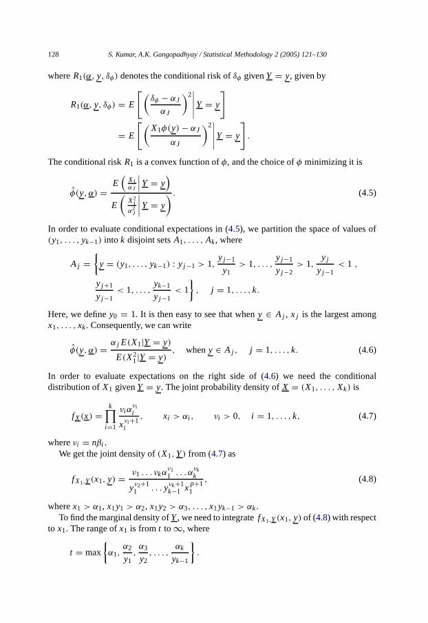
128 S. Kumar, A.K. Gangopadhyay / Statistical Methodology 2 (2005) 121–130

whereR1(α, y, δφ) denotes the conditional risk ofδφ givenY = y, given by

R1(α, y, δφ) = E

[(δφ − αJ

αJ

)2∣∣∣∣∣Y = y

]

= E

[(X1φ(y) − αJ

αJ

)2∣∣∣∣∣Y = y

].

The conditional riskR1 is a convex function ofφ, and the choice ofφ minimizing it is

φ(y, α) =E(

X1αJ

∣∣∣Y = y)

E

(X2

1α2

J

∣∣∣∣Y = y

) . (4.5)

In order to evaluate conditional expectations in (4.5), we partition the space of values of(y1, . . . , yk−1) into k disjoint setsA1, . . . , Ak, where

Aj ={

y = (y1, . . . , yk−1) : yj −1 > 1,yj −1

y1> 1, . . . ,

yj −1

yj −2> 1,

yj

yj −1< 1 ,

yj +1

yj −1< 1, . . . ,

yk−1

yj −1< 1

}, j = 1, . . . , k.

Here, we definey0 = 1. It is then easy to see that wheny ∈ Aj , x j is the largest amongx1, . . . , xk. Consequently, we can write

φ(y, α) = α j E(X1|Y = y)

E(X21|Y = y)

, wheny ∈ Aj , j = 1, . . . , k. (4.6)

In order to evaluate expectations on the right side of (4.6) we need the conditionaldistribution of X1 givenY = y. Thejoint probability density ofX = (X1, . . . , Xk) is

fX(x) =k∏

i=1

νi ανii

xνi +1i

, xi > αi , νi > 0, i = 1, . . . , k, (4.7)

whereνi = nβi .We get the joint density of(X1, Y) from (4.7) as

fX1,Y(x1, y) = ν1 . . . νkαν11 . . . α

νkk

yν2+11 . . . yνk+1

k−1 x p+11

, (4.8)

wherex1 > α1, x1y1 > α2, x1y2 > α3, . . . , x1yk−1 > αk.To find the marginal density ofY, we need to integratefX1,Y(x1, y) of (4.8) with respect

to x1. The range ofx1 is from t to ∞, where

t = max

{α1,

α2

y1,α3

y2, . . . ,

αk

yk−1

}.

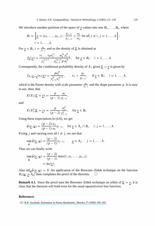
S. Kumar, A.K. Gangopadhyay / Statistical Methodology 2 (2005) 121–130 129

We introduce another partition of the space ofy-values into setsB1, . . . , Bk, where

Bi ={

y = (y1, . . . , yk−1) : yi−1

yj −1≤ αi

α jfor all j �= i , j = 1, . . . , k

};

i = 1, . . . , k.

For y ∈ Bi , t = αiyi−1

and so the density ofY is obtained as

fY(y) = ν1 . . . νkαν11 . . . α

νkk yp

i−1

yν2+11 . . . yνk+1

k−1 p αpi

, for y ∈ Bi ; i = 1, . . . , k.

Consequently, the conditional probability density ofX1 givenY = y is given by

fX1|Y=y(x1|y) = pαpi

ypi−1x p+1

1

, x1 >αi

yi−1, if y ∈ Bi ; i = 1, . . . , k,

which is the Pareto density with scale parameterαiyi−1

and the shape parameterp. It is easyto see, then, that

E(X1|Y = y) = p

(p − 1)

αi

yi−1,

and

E(X21|Y = y) = p

(p − 2)

α2i

y2i−1

, for y ∈ Bi .

Using theseexpectations in (4.6), we get

φ(y, α) = (p − 2)

(p − 1)

α j

αiyi−1, for y ∈ Aj ∩ Bi , i , j = 1, . . . , k.

Fixing j and varying over alli �= j , we seethat

supα

φ(y, α) = (p − 2)

(p − 1)yj −1, y ∈ Aj , j = 1, . . . , k.

Thus we can finally write

supα

φ(y, α) = (p − 2)

(p − 1)max{1, y1, . . . , yk−1}.

= φ0(y).

Also infαφ(y, α) = 0. An application of the Brewster–Zidek technique on the functionR1(α, y, δφ) then completes the proof of the theorem. �

Remark 4.1. Since the proof uses the Brewster–Zidek technique on orbits ofY = y, it isclear that the theorem will hold even for the usual squared error loss function.

References

[1] B.R. Asrabadi, Estimation in Pareto distribution, Metrika 37 (1990) 199–205.

130 S. Kumar, A.K. Gangopadhyay / Statistical Methodology 2 (2005) 121–130

[2] R.R. Bahadur, A.I. Goodman, Impartial decision rules and sufficient statistics, Ann. Math. Statist. 23 (1952)553–562.

[3] J.O. Berger, B. Mandelbrot, A new model for error clustering in telephone circuits, IBM J. Res. Dev. 7(1963) 224–236.

[4] J.F. Brewster, J.V. Zidek, Improving on equivariant estimators, Ann. Statist. 2 (1974) 21–38.[5] D.J. Charek, A.H. Moore, J.W. Coleman, A comparison of estimation techniques for the three parameter

Pareto distribution, Comm. Statist. Theory Methods 17 (4) (1988) 1394–1407.[6] A. Cohen, H.B. Sackrowitz, Estimating the meanof the selected population, in: S.S. Gupta, J.O. Berger

(Eds.), Statistical Decision Theory and Related Topics-III, vol. 1, Academic Press, New York, 1982,pp. 243–270.

[7] R.C. Dahiya, Estimation of the mean of the selected population, J. Amer. Statist. Assoc. 69 (1974) 226–230.[8] H.T. Davis, M.L. Feldstein, The generalized Pareto law as a model for progressively censored survival data,

Biometrika 66 (1979) 299–306.[9] M.L. Eaton, Some optimum properties of ranking procedures, Ann. Math. Statist. 38 (1967) 124–137.

[10] E.C. Freiling, A comparison of the fallout mass-size distributions calculated by lognormal and power lawmodels, U.S. Naval Radiological Defence Laboratory, San Francisco, 1966 (AD-646019).

[11] C.M. Harris, The Pareto distributions as a queue service discipline, Oper. Res. 16 (1968) 307–313.[12] J.R.M. Hosking, J.R. Wallis, Parameter and quantile estimation for the generalized Pareto distribution,

Technometrics 29 (3) (1987) 339–349.[13] H.K. Hsieh, On estimating the mean of the selected population with unknown variance, Comm. Statist.

Theory Methods 10 (1981) 1869–1878.[14] N.L. Johnson, S. Kotz, Continuous univariate distributions-I, John Wiley and Sons, New York, 1970.[15] M.D. Kern, Minimum variance unbiased estimation in the Pareto distribution, Metrika 30 (1983) 15–19.[16] S. Kumar, A. Kar, Estimating quantiles of a selected exponential population, Statist. Probab. Lett. 26 (2001)

9–19.[17] E.L. Lehmann, On a theorem of Bahadur and Goodman, Ann. Math. Statist. 37 (1966) 1–6.[18] H.J. Malik, Estimation of the parameters ofthe Pareto distribution, Metrika 15 (1970) 126–132.[19] N. Misra, E.C. van der Meulen, On estimation following selection from nonregular distributions, Comm.

Statist. Theory Methods 30 (12) (2001) 2543–2561.[20] V. Pareto, Cours d’ Economic Politique, Rouge and Cie, Lansanne and Paris, 1897.[21] H.B. Sackrowitz, E. Samuel-Cahn, Estimation of the mean of a selected negative exponential population,

J.R. Stat. Soc. Ser. B 46 (1984) 242–249.[22] P. Vellaisamy, Inadmissibility results for the selected scale parameters, Ann. Statist. 20 (1992) 2183–2191.[23] P. Vellaisamy, S. Kumar, D. Sharma, Estimating the mean of the selected uniform population, Comm. Statist.

Theory Methods 17 (10) (1988) 3447–3475.[24] P. Vellaisamy, D. Sharma, Estimating the meanof the selected gamma population, Comm. Statist. Theory

Methods 17 (8) (1988) 2797–2817.